methods for inference in large multiple-equation markov-switching
TRANSCRIPT

WORKING PAPER SERIESFED
ERAL
RES
ERVE
BAN
K of A
TLAN
TA
Methods for Inference in Large Multiple-Equation Markov-Switching Models Christopher A. Sims, Daniel F. Waggoner and Tao Zha Working Paper 2006-22 November 2006

The authors thank Tim Cogley, John Geweke, Michel Juillard, Ulrich Mueller, and Frank Schorfheide for helpful discussions and comments. Eric Wang provided excellent research assistance in computation on the Linux operating system. The authors also acknowledge the technical support on parallel and grid computation from the Computing College of the Georgia Institute of Technology. The views expressed here are the authors’ and not necessarily those of the Federal Reserve Bank of Atlanta or the Federal Reserve System. Any remaining errors are the authors’ responsibility. Please address questions regarding content to Christopher A. Sims, Professor of Economics and Banking, Department of Economics, 104 Fisher Hall, Princeton University, Princeton, NJ 08544-1021, 609-258-4033, [email protected]; Daniel Waggoner, Research Economist and Associate Policy Adviser, Research Department, Federal Reserve Bank of Atlanta, 1000 Peachtree Street, N.E., Atlanta, GA 30309-4470, 404-498-8278, [email protected]; or Tao Zha, Research Economist and Senior Policy Adviser, Research Department, Federal Reserve Bank of Atlanta, 1000 Peachtree Street, N.E., Atlanta, GA 30309-4470, 404-498-8353, [email protected]. Federal Reserve Bank of Atlanta working papers, including revised versions, are available on the Atlanta Fed’s Web site at www.frbatlanta.org. Click “Publications” and then “Working Papers.” Use the WebScriber Service (at www.frbatlanta.org) to receive e-mail notifications about new papers.
FEDERAL RESERVE BANK of ATLANTA WORKING PAPER SERIES
Methods for Inference in Large Multiple-Equation Markov-Switching Models Christopher A. Sims, Daniel F. Waggoner, and Tao Zha Working Paper 2006-22 November 2006
Abstract: The inference for hidden Markov chain models in which the structure is a multiple-equation macroeconomic model raises a number of difficulties that are not as likely to appear in smaller models. One is likely to want to allow for many states in the Markov chain without allowing the number of free parameters in the transition matrix to grow as the square of the number of states but also without losing a convenient form for the posterior distribution of the transition matrix. Calculation of marginal data densities for assessing model fit is often difficult in high-dimensional models and seems particularly difficult in these models. This paper gives a detailed explanation of methods we have found to work to overcome these difficulties. It also makes suggestions for maximizing posterior density and initiating Markov chain Monte Carlo simulations that provide some robustness against the complex shape of the likelihood in these models. These difficulties and remedies are likely to be useful generally for Bayesian inference in large time-series models. The paper includes some discussion of model specification issues that apply particularly to structural vector autoregressions with a Markov-switching structure. JEL classification: C32, C52, E52 Key words: volatility, coefficient changes, discontinuous shifts, Lucas critique, independent Markov processes

METHODS FOR INFERENCE IN LARGE MULTIPLE-EQUATIONMARKOV-SWITCHING MODELS
I. INTRODUCTION
This paper extends the methods of Hamilton (1989), Chib (1996), and Kim and Nelson
(1999) to multiple equation models. In such large models, a variety of modeling choices,
not needed in smaller models, are required to control dimensionality. We provide sug-
gestions for ways to keep these models tractable. Some of the suggestions are specific to
structural VAR’s, but some apply more generally.
The first part of the paper considers a large class of restrictions on the parameters in the
transition matrix. This class maintains a standard posterior density form for the free param-
eters in the transition matrix. Although one could directly derive and code up the posterior
density function case by case, we propose a general interface that is straightforward for
researchers to automate potentially complex restrictions by simply expressing them in a
convenient matrix form. A number of examples are employed to illustrate how such an
interface matrix can be formed.
The second part of the paper describes a general structural VAR Markov-switching
framework that allows four key elements: (1) simultaneity, (2) over-identifying restrictions
on both contemporaneous coefficients and lag structure, (3) switching among regimes for
the residual covariance matrix independently from switching among regimes for equation
coefficients and (4) switching among regimes for coefficients in one structural equation
(e.g., monetary policy) independently from switching among those for coefficients in other
equations. Our framework is particularly useful in addressing questions related to the cur-
rent debate on whether monetary policy and the private sector’s behavior have significantly
changed in recent history, and indeed most of the methods described here were either ap-
plied in Sims and Zha (2006) or are extensions of methods that were applied in that paper.1
When one evaluates marginal data densities using the Modified Harmonic Means (MHM)
method, a typical choice of a weighting function is a Gaussian density function constructed1For the debate on monetary history, consult Cogley and Sargent (2002), Canova and Gambetti (2004),
Beyer and Farmer (2004), Cogley and Sargent (2005), Primiceri (2005), and Sims and Zha (2006).1

METHODS FOR LARGE SWITCHING MODELS 2
from the first two sample moments of the posterior distribution. If the posterior distribution
is very non-Gaussian, however, such a weighting function can be a very poor approxima-
tion. We propose a more general weighting function that aims at dealing with the non-
Gaussian shape of the posterior distribution. We show that our new weighting function
works well for the high-dimensional models studied by this paper.
The rest of the paper is organized as follows.
Section II develops a method for estimating Markov-switching models with a certain
class of linear restrictions on transition matrices. This class includes restrictions that apply
when there are independently evolving states, as well as other forms of restriction that are
likely to prove useful in applications.
Section III develops tools for estimation and inference of both identified and unrestricted
switching vector autoregression (VAR) models with transition matrices satisfying restric-
tions in this class.
In Section IV, we describe a block-wise optimization method for estimating these mod-
els. The method proves, in this application, to be much more computationally efficient than
the expectation-maximization (EM) algorithm, which has been widely used in similar, but
smaller, models.
In Section V, we show that the usual implementation of the Modified Harmonic Mean
method (MHM) for calculating marginal data densities runs into severe difficulties in these
models, and we suggest a variation on the MHM method that works much better.
A three-variable VAR application to the post-war US data is presented in Section VI.
And Section VII concludes.
II. MARKOV-SWITCHING MODEL
II.1. Distributional assumptions. Let (Yt ,Zt ,θ ,Q,St) be a collection of random variables
where
Yt = (y1, · · · ,yt) ∈ (Rn)t ,
Zt = (z1, · · · ,zt) ∈ (Rm)t ,
θ = (θi)i∈H ∈ (Rr)h ,
Q =(qi, j
)(i, j)∈H×H ∈ Rh2
,

METHODS FOR LARGE SWITCHING MODELS 3
St = (s0, · · · ,st) ∈ Ht+1,
STt+1 = (st+1, · · · ,sT ) ∈ HT−t ,
and H is a finite set with h elements and is usually taken to be the set 1, · · · ,h. The vector
yt contains the endogenous variables and the vector zt contains the exogenous variables.
Our analysis, however, encompass the case in which there are no exogenous variables.
The matrix Q is a Markov transition matrix and qi, j is the probability that st is equal to i
given that st−1 is equal to j. The matrix Q is restricted to satisfy
qi, j ≥ 0 and ∑i∈H
qi, j = 1.
We shall follow the convention that if u and v are random vectors for which a density
function exists, p(u,v) denotes the density function. The marginal and conditional density
functions are expressed as
p(v) =∫
p(u,v)du,
and
p(u | v) =p(u,v)∫p(u,v)du
.
We assume that p(u,v) is integrable. Hence, p(u | v) and p(v) will exist for almost all
v. The objects θ and Q are parameters, Yt and Zt are observed data, and St can be con-
sidered either a sequence of unobserved variables or a vector of nuisance parameters. We
assume that (Yt ,Zt ,θ ,Q,St) has a joint density function p(Yt ,Zt ,θ ,Q,St), where we use the
Lebesgue measure2 on (Rn)t × (Rm)t × (Rr)h×Rh2and the counting measure on Ht+1.
This density satisfies the following conditions.
Condition 1.
p(st | Yt−1,Zt−1,θ ,Q,St−1) = qst ,st−1
for t > 0.
Condition 2.
p(yt | Yt−1,Zt ,θ ,Q,St) = p(yt | Yt−1,Zt ,θ ,st)
for t > 0.2Instead of the Lebesgue measure, any sigma finite measure on Rn and Rm can be used as long as the
product measure is used on (Rn)t and (Rm)t .

METHODS FOR LARGE SWITCHING MODELS 4
Condition 3.
p(zt | Yt−1,Zt−1,θ ,Q,St) = p(zt | Yt−1,Zt−1) .
Condition 1 states formally that the sequence St evolves according to an exogenous
Markov process with the transition matrix Q. Condition 2 is needed for obtaining a stan-
dard posterior density function of Q conditional on ST .3 Condition 3 ensures that zt is an
exogenous variable.
II.2. Propositions. From Conditions 1 - 3, one can prove the following propositions (the
proofs can be found in Hamilton (1989), Chib (1996), and Kim and Nelson (1999)). These
propositions are used throughout the rest of this paper.
Proposition 1.
p(st | Yt−1,Zt−1,θ ,Q) = ∑st−1∈H
qst ,st−1 p(st−1 | Yt−1,Zt−1,θ ,Q)
for t > 0.
Proposition 2.
p(st | Yt ,Zt ,θ ,Q) =p(yt | Yt−1,Zt ,θ ,st) p(st | Yt−1,Zt−1,θ ,Q)
∑st−1∈H p(yt | Yt−1,Zt ,θ ,st) p(st | Yt−1,Zt−1,θ ,Q)
for t > 0.
Proposition 3.
p(st | Yt ,Zt ,θ ,Q,st+1) = p(st | YT ,ZT ,θ ,Q,ST
t+1)
for 0≤ t < T .
Proposition 4.
p(yt ,zt | Yt−1,Zt−1,θ ,Q,ST ) = (yt ,zt | Yt−1,Zt−1,θ ,Q,St)
for 0 < t ≤ T .
3This tractable result no longer holds for most regime-switching rational expectations models
(Farmer, Waggoner, and Zha, 2006). In that case, the Metropolis algorithm may be used instead. We thank
Tim Cogley for bringing our attention to this point.

METHODS FOR LARGE SWITCHING MODELS 5
II.3. Restrictions on Q. An important part of this paper is to consider a wide range of
restrictions on Q while maintaining the standard form of its posterior probability density
function. We first consider a general class of linear restrictions. This class includes exclu-
sion restrictions, fixing certain transition probabilities at a known non-zero constant, and
keeping certain transition probabilities proportional to one another. The second class of
restrictions is nonlinear and involves a tensor product of transition matrices to allow for
independent Markov processes.
II.3.1. Linear restrictions on Q. For 1 ≤ j ≤ h, let q j be the jth column of Q and let q be
an h2-dimensional column vector stacking these q j’s. If Q is unrestricted, the likelihood as
a function of q j is proportional to a Dirichlet density. The same is true of the posterior if
the prior on q j is of Dirichlet and the initial distribution on s0 does not depend on q. We
shall consider linear restrictions on q that preserve this property.
For 1 ≤ j ≤ v, let w j be a d j-dimensional vector, where v may be greater or less than h
and the elements of w j are non-negative and sum to one. Let w be a d-dimensional column
vector stacking w j’s, where d = ∑vj=1 d j. We describe the linear restrictions on q by
q = Mw, (1)
where M is an h2×d matrix such that
M =
M1,1 · · · M1,v... . . . ...
Mh,1 · · · Mh,v
.
Mi, j is an h×d j matrix and satisfies the following two conditions.
Condition 4. Let λi, j,r be the sum of the elements in any column of Mi, j, where the column
is indexed by r ∈ 1, . . . ,d j. Then, ∑vj=1 λi, j,r = 1.
Condition 5. All the elements of M are non-negative and each row of M has at most one
non-zero element.
Condition 4 is necessary to ensure that the elements of q j sum to one. Condition 5
ensures that the elements of q j are positive and that the likelihood as a function of w j has
the Dirichlet density form. It follows from these conditions that one may assume without

METHODS FOR LARGE SWITCHING MODELS 6
loss of generality that d j ≤ h and d ≤ h2. Our class of restrictions on Q encompasses most
examples discussed in the literature.
Clearly one could work directly on the transition matrix Q that satisfies the restrictions
specified by (1), without explicitly constructing the transformation matrix M in the manner
of Conditions 4 and 5. However, if restrictions are complicated and a researcher does not
want to derive and code up the posterior density of the free elements in the transition matrix
each time when a new application is studied, the setup (1) provides a way to automate the
handling of different kinds of restrictions in one convenient framework. Furthermore, when
the researcher chooses to use our computer program, the general-purpose interface matrix
M in (1) as one of inputs for the program becomes very handy and easy to implement.4 In
the following we illustrate how to construct the transformation matrix M for a number of
useful examples. Some of the examples are used to show how to keep the number of free
parameters in the transition matrix from growing too fast as the number of states increases.
Example 1. Sims (1999) discusses a structural break with an irreversible regime change. In
a two-state case where the second state is absorbing or irreversible, we have
M =
1 0 0
0 1 0
0 0 0
0 0 1
,
where v = 2, d1 = 2, and d2 = 1. In general, exclusion restrictions of the form qi, j = 0
require that the (h( j−1)+ i)th row of M j be zero.
Example 2. A symmetric jumping among states considered by Sims (2001) introduces a
parsimonious parameterization of Q to avoid over-parameterization. The transition matrix
studied by Sims (2001) has the following form
Q =
π1 (1−π2)/2 0
1−π1 π2 1−π3
0 (1−π2)/2 π3
, (2)
4The software is available at http://home.earthlink.net/ tzha02/ProgramCode/programCode.html.

METHODS FOR LARGE SWITCHING MODELS 7
where π1, π2, and π3 are free parameters to be estimated. These restrictions can be ex-
pressed as
M1,1 =
1 0
0 1
0 0
, M2,2 =
0 1/2
1 0
0 1/2
, M3,3 =
0 0
1 0
0 1
,
and Mi, j = 0 for i 6= j, where v = 3 and d1 = d2 = d3 = 2.
Example 3. Consider a three-state example where the third state is irreversible. A transition
to this absorbing state occurs only from the second state and the transition probability is
1/4. It follows that the transition matrix is of the form
q1,1 q1,2 0
q2,1 q2,2 0
0 1/4 1
.
This example is used to show how to implement exclusion restrictions and, more gener-
ally, how to handle the case in which some of the transition probabilities are known. To put
these restriction in the matrix form of M, let v = 3, d1 = 2, d2 = 2, and d3 = 1. The 9×5
matrix M is
1 0 0 0 0
0 1 0 0 0
0 0 0 0 0
0 0 3/4 0 0
0 0 0 3/4 0
0 0 0 0 1/4
0 0 0 0 0
0 0 0 0 0
0 0 0 0 1
.
Example 4. This example pertains to incremental changes in the model parameters (Cogley and Sargent,
2005).5 This kind of parameter drift can be approximated arbitrarily well by expanding the
number of states while containing the elements of Q in a much smaller dimension. Our
5See also Sims (1993); Cogley and Sargent (2002); Stock and Watson (2003); Canova and Gambetti
(2004); Primiceri (2005).

METHODS FOR LARGE SWITCHING MODELS 8
approach has advantage over that of Cogley and Sargent (2005) because it allows for oc-
casional discontinuous shifts in regime as well as frequent, incremental changes in param-
eters. One way to achieve this task is to concentrate weight on the diagonal of Q (Zha,
In press). Specifically, one can express incremental increases and discontinuous jumps
among n+1 states as
Q =
π1 β2α2(1−π2) . . . βn+1αnn+1(1−πn+1)
β1α1(1−π1) π2 . . . βn+1αn−1n+1 (1−πn+1)
β1α21 (1−π1) β2α2(1−π2) . . . βn+1αn−2
n+1 (1−πn+1)
. . . . . . . . . . . .
β1αn1 (1−π1) β2αn−1
2 (1−π2) . . . πn+1
,
where πi is a free parameter and 0 < αi < 1 is taken as a given. The restrictions can be
written as
M1,1 =
1 0
0 β1α1
0 β1α21
. . . . . .
0 β1αn1
, M2,2 =
0 β2α2
1 0
0 β2α2
. . . . . .
0 β2αn−12
, . . . , Mn+1,n+1 =
0 βn+1αnn+1
0 βn+1αn−1n+1
0 βn+1αn−2n+1
. . . . . .
1 0
,
where the values of αi and βi must be such that elements in each column of Mi,i sum up to
1. Note that v = n+1, d1 = · · ·= dn+1 = 2, and Mi, j = 0 for i 6= j.
Example 5. The above example shows that we can reduce a large number of elements in the
transition matrix to free parameters whose dimension is equal to the number of states. The
class of linear restrictions specified in (1) enables us to reduce a number of free parameter
even further. Consider an h×h transition matrix Q in the form of
a b/2 · · · 0 0
b a . . . ......
0 b/2 . . . b/2 0...
... . . . a b
0 0 · · · b/2 a
.
This restricted transition matrix implies that when we are in state j, the probability of
moving to state j−1 or j +1 is symmetric and independent of j. Let v = 1 and d1 = 2. We

METHODS FOR LARGE SWITCHING MODELS 9
can express this restriction as
M1,1 =
1 0
0 1
0 0...
...
0 0
, Mh,1 =
0 0...
...
0 0
1 0
0 1
,
and for 1 < i < h, the h×2 matrix Mi,1 is zero except for a block centered at the ith row that
has the form
0 1/2
1 0
0 1/2
.
In general, our setup is flexible enough to handle more elaborate cases where the jumping
probabilities are not symmetric or independent or where a variable jumps from a state to
nearby (but not adjacent) states.
Example 6. The original approach of Hamilton (1989) makes it explicit for the model pa-
rameters to depend on not only the current state but also the previous state. This dependence
on the past state can be easily modelled in our framework. Suppose the original state vari-
able, denoted by sot , takes on two values and has the transition matrix P =
(pi, j
). Let the
composite state variable, st = sot ,s
ot−1, consist of a pair of current and previous states.
There will be four possibilities for st and the overall transition matrix Q must be of the
form
(st−1,st−2)
(st ,st−1)
(1,1) (1,2) (2,1) (2,2)
(1,1) p1,1 p1,1 0 0
(1,2) 0 0 p1,2 p1,2
(2,1) p2,1 p2,1 0 0
(2,2) 0 0 p2,2 p2,2

METHODS FOR LARGE SWITCHING MODELS 10
To express this restricted Q in the form of (1), we have ν = 2, d1 = d2 = 2, M1,2 = M2,2 =
M3,1 = M4,1 = 0,
M1,1 = M2,1 =
1 0
0 0
0 1
0 0
, and M2,2 = M4,2 =
0 0
1 0
0 0
0 1
.
II.3.2. Independent Markov processes. We now consider the case in which there are κ
independent Markov processes. Let h = ∏κk=1 hk, H = ∏κ
k=1 Hk where Hk =
1, · · · ,hk
,
and st =(s1t , · · · ,sκ
t)
where skt ∈ Hk. The transition matrix Q is therefore restricted to the
form
Q = Q1⊗·· ·⊗Qκ
where Qk =(
qki, j
)is an hk×hk matrix such that
qki, j ≥ 0 and ∑
i∈Hk
qki, j = 1.
The tensor product representation of Q implies that if i =(i1, · · · , iκ)∈H and j =
(j1, · · · , jκ)∈
H, then qi, j = ∏κk=1 qk
ik, jk . Conditional on Q, the composite (overall) Markov process st con-
sists of κ independent Markov processes skt . If Q were not restricted to this tensor product
representation, then it would contain(∏κ
k=1 hk)(
∏κk=1 hk−1
)parameters. With this non-
linear restriction, there are only ∑κk=1 hk (
hk−1)
parameters – a substantial reduction.
One can combine the two types of restrictions by imposing the linear restrictions on
each Qk individually. Specifically, we let qk be the(hk
)2-dimensional vector obtained
by stacking the columns of Qk, wkj be a dk
j -dimensional vector whose elements are non-
negative and sum to one for 1 ≤ j ≤ vk, wk be the the dk-dimensional vector obtained by
stacking the wkj where dk = ∑vk
j=1 dkj , and Mk be a
(hk
)2×dk matrix satisfying Conditions
4 and 5. It follows from Section II.3.1 that Qk can restricted by requiring
qk = Mkwk.
In the remainder of this paper, we simplify the notation by suppressing the superscript
denoting which of the independent Markov state variables is under consideration. It is
important to remember, however, that all of the results apply to a product of independent
Markov state variables by simply adding the superscript k in appropriate places.

METHODS FOR LARGE SWITCHING MODELS 11
II.4. Prior. In this section we describe the prior on all the model parameters. We begin
with the prior on Q if Q is unrestricted. For 1≤ i, j ≤ h, let αi, j be a positive number. The
prior on Q is of the Dirichlet form
p(Q) = ∏j∈H
[(Γ
(∑i∈H αi, j
)
∏i∈H Γ(αi, j
))×∏
i∈H
(qi, j
)αi, j−1
], (3)
where Γ(·) denotes the standard gamma function.
We now consider the restricted transition matrix Q as discussed in Section II.3.1. Denote
w j =[w1, j, · · · ,wd j, j
]′. The prior on w j is of the Dirichlet form
Γ(
∑d ji=1 βi, j
)
∏d ji=1 Γ
(βi, j
)d j
∏i=1
(wi, j
)βi,, j−1 (4)
where βi, j > 0. The prior on Q can be derived via (1).
The joint prior density for θ ,Q,ST is
p(θ ,Q,ST ) = p(θ ,Q) p(s0 | θ ,Q)T
∏t=1
p(st | θ ,Q,St−1)
By Condition 1, p(st | θ ,Q,St−1) = qst ,st−1 . We assume that the prior on θ is independent
of the prior on Q and that p(s0 | θ ,Q) = 1h for every s0 ∈ H.6 The resulting prior has the
following form
p(θ ,Q,ST ) =p(θ) p(Q)
h
T
∏t=1
qst ,st−1. (5)
II.5. Likelihood. Using Proposition 4 and Conditions 2 and 3, one can show that the joint
density of YT and ZT conditional on θ and Q is
p(YT ,ZT | θ ,Q) =T
∏t=1
p(yt ,zt | Yt−1,Zt−1,θ ,Q)
Note
p(yt ,zt | Yt−1,Zt−1,θ ,Q) = ∑st∈H
p(yt ,zt ,st | Yt−1,Zt−1,θ ,Q)
= ∑st∈H
p(yt ,zt | Yt−1,Zt−1,θ ,Q,st) p(st | Yt−1,Zt−1,θ ,Q)
6The conventional assumption for p(s0 | θ ,Q) is the ergodic distribution of Q, if it exists. This convention,
however, makes the conditional posterior distribution of Q an unknown and complicated one.

METHODS FOR LARGE SWITCHING MODELS 12
and
p(yt ,zt | Yt−1,Zt−1,θ ,Q,st)
= p(yt | Yt−1,Zt ,θ ,Q,st) p(zt | Yt−1,Zt−1,θ ,Q,st)
= p(yt | Yt−1,Zt ,θ ,st) p(zt | Zt−1) ,
it follows that
p(YT ,ZT | θ ,Q) =T
∏t=1
p(zt | Zt−1)T
∏t=1
[∑
st∈Hp(yt | Yt−1,Zt ,θ ,st) p(st | Yt−1,Zt−1,θ ,Q)
]
= p(ZT )T
∏t=1
[∑
st∈Hp(yt | Yt−1,Zt ,θ ,st) p(st | Yt−1,Zt−1,θ ,Q)
]
Conditional on the vector of exogenous variables Zt , the likelihood of YT is
p(YT | ZT ,θ ,Q) =T
∏t=1
[∑
st∈Hp(yt | Yt−1,Zt ,θ ,st) p(st | Yt−1,Zt−1,θ ,Q)
](6)
This likelihood can be evaluated recursively, using Propositions 1 and 2.
II.6. Posterior distribution. By the Bayes rule, it follows from (5) and (6) that the poste-
rior distribution of (θ ,Q) is
p(θ ,Q | YT ,ZT ) ∝ p(θ ,Q)p(YT | ZT ,θ ,Q). (7)
The posterior density p(θ ,Q |YT ,ZT ) is unknown and complicated; the MCMC simulation
directly from this distribution can be inefficient and problematic. One can, however, use the
idea of Gibbs sampling to obtain the empirical joint posterior density p(θ ,Q,ST | YT ,ZT )
by sampling alternately from the following conditional posterior distributions:
p(ST | YT ,ZT ,θ ,Q),
p(Q | YT ,ZT ,ST ,θ),
p(θ | YT ,ZT ,Q,ST ).
Simulation from the conditional posterior density p(θ | YT ,ZT ,Q,ST ) is model-dependent,
which we will discuss in Section III. In this section we study the first two conditional
posterior distributions.

METHODS FOR LARGE SWITCHING MODELS 13
II.6.1. Conditional posterior distribution of ST . The distribution of ST conditional on YT ,
ZT , θ , and Q is
p(ST | YT ,ZT ,θ ,Q) = p(sT | YT ,ZT ,θ ,Q) p(ST−1 | YT ,ZT ,θ ,Q,ST
T)
= p(sT | YT ,ZT ,θ ,Q)T−1
∏t=0
p(st | YT ,ZT ,θ ,Q,ST
t+1)
where STt+1 = st+1, · · · ,sT. From Proposition 3,
p(st | YT ,ZT ,θ ,Q,ST
t+1)
= p(st | Yt ,Zt ,θ ,Q,st+1)
=p(st ,st+1 | Yt ,Zt ,θ ,Q)
p(st+1 | Yt ,Zt ,θ ,Q)
=p(st+1 | Yt ,Zt ,θ ,Q,st) p(st | Yt ,Zt ,θ ,Q)
p(st+1 | Yt ,Zt ,θ ,Q)
=qst+1,st p(st | Yt ,Zt ,θ ,Q)
p(st+1 | Yt ,Zt ,θ ,Q)
The conditional density p(st | YT ,ZT ,θ ,Q,ST
t+1)
is straightforward to evaluate according
to Propositions 1 and 2, . Starting with sT and working backward, we can easily sample
ST from the posterior conditional on YT ,ZT ,θ ,Q by using the following fact
p(st | YT ,ZT ,θ ,Q) = ∑st+1∈H
p(st ,st+1 | YT ,ZT ,θ ,Q)
= ∑st+1∈H
p(st | YT ,ZT ,θ ,Q,st+1) p(st+1 | YT ,ZT ,θ ,Q)
= ∑st+1∈H
p(st | Yt ,Zt ,θ ,Q,st+1) p(st+1 | YT ,ZT ,θ ,Q) .
Note that this density can also be evaluated recursively.
II.6.2. Conditional posterior distribution of Qk. The conditional posterior density of Q
derives directly from the conditional posterior density of the free parameters w j.7 It follows
from Condition 1 and the prior (4) that
p(w j | YT ,ZT ,θ ,ST
)∝
d j
∏i=1
(wi, j
)ni, j+βi, j−1
where ni, j is the number of transitions from st−1 = s to st = r for Mr, j(s, i) > 0, where
Mr, j(s, i) is the sth-row and ith-column element of the submatrix Mr, j.
7To be consistent with Section II.4, we suppress the superscript k that indicates a particular Markov process
under study.

METHODS FOR LARGE SWITCHING MODELS 14
III. STRUCTURAL VAR MODELS
The methodology developed thus far has been used by Rubio-Ramírez, Waggoner, and Zha
(2006) and Sims and Zha (2006) to study a class of simultaneous-equation multivariate dy-
namic models that are commonly used for policy analysis. In this section, we develop and
detail the econometric methods specific to these types of models.
III.1. Likelihood. We consider a class of models of the following form:
y′tA(st) =ρ
∑i=1
y′t−iAi (st)+ z′tC (st)+ ε ′t Ξ−1 (st) , for 1≤ t ≤ T , (8)
where
• ρ is a lag length;
• yt is an n-dimensional column vector of endogenous variables at time t;
• zt is an m-dimensional column vector of exogenous and deterministic variables at
time t;
• εt is an n-dimensional column vector of unobserved random shocks at time t;
• For 1≤ k ≤ h, A(k) is an invertible n×n matrix and Ai (k) is an n×n matrix;
• For 1≤ k ≤ h, C (k) is an m×n matrix;
• For 1≤ k ≤ h, Ξ(k) is an n×n diagonal matrix.
For the rest of the paper we take the initial conditions y0, · · · ,y1−ρ as given. Let
xtpn×1
=
yt−1...
yt−ρ
zt
and F (st)(pn+m)×n
=
A1 (st)...
Aρ (st)
C (st)
.
Then (8) can be written in the compact form:
y′tA(st) = x′tF (st)+ ε ′t Ξ−1 (st) , for 1≤ t ≤ T (9)
METHODS FOR LARGE SWITCHING MODELS 15
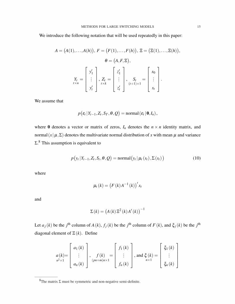
We introduce the following notation that will be used repeatedly in this paper:
A =(A(1), . . . ,A(h)
), F =
(F(1), . . . ,F(h)
), Ξ =
(Ξ(1), . . . ,Ξ(h)
),
θ =(A,F,Ξ
),
Ytt×n
=
y′1...
y′t
, Zt
t×k=
z′1...
z′t
, St
(t+1)×1=
s0...
st
.
We assume that
p(εt |Yt−1,Zt ,ST ,θ ,Q
)= normal(εt |0, In) ,
where 0 denotes a vector or matrix of zeros, In denotes the n× n identity matrix, and
normal(x |µ ,Σ) denotes the multivariate normal distribution of x with mean µ and variance
Σ.8 This assumption is equivalent to
p(yt |Yt−1,Zt ,St ,θ ,Q
)= normal
(yt |µt (st) ,Σ(st)
)(10)
where
µt (k) =(F (k)A−1 (k)
)′xt
and
Σ(k) =(A(k)Ξ2 (k)A′ (k)
)−1
Let a j (k) be the jth column of A(k), f j (k) be the jth column of F (k), and ξ j (k) be the jth
diagonal element of Ξ(k). Define
a(k)n2×1
=
a1 (k)...
an (k)
, f (k)
(pn+m)n×1=
f1 (k)...
fn (k)
, and ξ (k)
n×1=
ξ1 (k)...
ξn (k)
8The matrix Σ must be symmetric and non-negative semi-definite.

METHODS FOR LARGE SWITCHING MODELS 16
It follows from (10) that
p(yt |Yt−1,Zt ,St ,θ ,Q
)= |Σ(st)|−
12 exp
(−1
2(yt −µ (st))
′Σ−1 (st)(yt −µ (st)))
= |A(st)Ξ(st)|exp(−1
2(y′tA(st)− x′tF (st)
)Ξ2 (st)
(A′ (st)yt −F ′ (st)xt
))
= |A(st)|n
∏j=1
∣∣ξ j (st)∣∣exp
(−ξ 2
j (st)2
(y′ta j (st)− x′t f j (st)
)2
).
We consider the case where the state variable st = [s1t s2t ] is a composite one such that
either s1t = s2t or s1t and s2t are independent random variables. The analytical results for
more complicated cases will follow directly. We let a j and f j depend on s1t and ξ j depend
on s2t . Thus, the conditional likelihood function p(yt |Yt−1,Zt ,St ,θ ,Q
)is equal to
|A(s1t)|n
∏j=1
∣∣ξ j (s2t)∣∣exp
(−ξ 2
j (s2t)2
(y′ta j (s1t)− x′t f j (s1t)
)2
). (11)
Given (11), the likelihood of YT can be formed by following (6).
III.2. A priori restrictions.
III.2.1. Restrictions on time variation. If we let all parameters vary across states, the num-
ber of free parameters in the model becomes impractically high when the system of equa-
tions is large or the lag length is long. For a typical quarterly model with 5 lags and 6
endogenous variables, for example, the number of parameters in F(s1t) is of order 180 for
each state. Given the post-war macroeconomic data, however, it is not uncommon to have
some states lasting for only a few years and thus the number of associated observations is
far less than 180 quarters. It is therefore essential to simplify the model by restricting the
degree of time variation in the model’s parameters. Such a restriction entails complexity
and difficulties that have not been dealt with in the simultaneous-equation literature.
To begin with, we rewrite F as
F(s1t)m×n
= G(s1t)m×n
+ Sm×n
A(s1t)n×n
. (12)
where
S =
In
0(m−n)×n
.

METHODS FOR LARGE SWITCHING MODELS 17
We let G be a collection of all G(k) for k = 1, . . . ,h1. If we place a prior distribution on
G(s1t) that has mean zero, the specification of S is consistent with the reduced-form random
walk feature implied by the existing Bayesian VAR models (Sims and Zha 1998). This type
of prior tends to imply that greater persistence (in the sense of a tighter concentration of the
prior on the random walk) is associated with smaller disturbance variances. This feature is
reasonable, as it is consistent with the idea that beliefs about the unconditional variance of
the data are not highly correlated with beliefs about the degree of persistence in the data.
Let g j(k) be the jth column of G(k). The time-variation restrictions imposed on g j(k)
can be generally expressed by two components, one being time varying and the other being
constant across states. Denote the first component by the rg, j × 1 vector gδ j(k) and the
second component by the h1rg, j×1 vector gψ j , where the subscripts δ j (k) and ψ j will be
discussed further in Section III.2.2. We express g j (k) for k = 1, . . . ,h1 in the form
diag([
g j(1)′ . . . g j(h1)′]′)
= diag([
g′δ j(1) . . . g′δ j(h1)
]′)diag
(gψ j
), (13)
where diag(x) is the diagonal matrix with the diagonal being the column vector x. The long
vector gψ j is formed by stacking h1 sub-vectors and the kth sub-vector corresponds to the
parameters in the kth state.
In this paper we focus on the following three cases of restricted time variations for a j(s1t)
and g j(s1t) for the jth equation where j∈1, . . . ,n, although our general method is capable
of dealing with other time variation cases.
a j(s1t)ξ j(s2t), gi j,`(s1t)ξ j(s2t), c j(s1t)ξ j(s2t) =
a j, gi j,`, c j Case I
a j ξ j(s2t), gi j,` ξ j(s2t), c j ξ j(s2t) Case II
a j(s1t)ξ j(s2t), gψi j,` gδi j(s1t) ξ j(s2t), c j(s1t)ξ j(s2t) Case III
, (14)
where gi j, `(s1t) is the element of g j(s1t) for the ith variable at the `th lag and c j(s1t) is a
vector of parameters corresponding to the exogenous variable zt in equation j. The param-
eter gψi j, ` is the element of gψ j for the ith variable at the `th lag in any state; it is constant
across states. The parameter gδi j(s1t) is the element of gδ j(s1t) for the ith variable in state
s1t at any lag. Thus, when the state s1t changes, gδi j(s1t) changes with variables but does
not vary across lags. The variability across variables when the sate changes is necessary

METHODS FOR LARGE SWITCHING MODELS 18
to allow long run (policy) responses to vary over time, while the restriction on the time
variation across lags is essential to prevent over-parameterization. The parameters a j, gi j, `,
and c j without the symbol (s1t) mean that these parameters are restricted to be independent
of state (i.e., constant across time).
In this setup, we include c j(k) in the stacked column vector gψ j . In principle, one could
include the time-varying parameter c j(k) as part of the time-varying component vector
gδ j(k). With the normalization c j(1) = 1, however, the likelihood function for c j(k) where
k ≥ 2 is so ill-behaved that our Gibbs sampler fails to work. Moreover, our reparameteri-
zation of grouping c j(k) in gψ j preserves the prior correlations between c j(k) and the other
lagged coefficients as implied by the Sims and Zha (1998) dummy-observation prior, an
important part of the prior specification. It is important to note that the other elements of
gψ j are restricted to be invariant to state.
Case I represents a traditional constant-parameter VAR equation, which has been dealt
with extensively in the literature and thus will not be a focal discussion of this paper. Case II
represents a structural equation with time-varying disturbance variances only. In this case,
ξ j(s2t) measures volatility for the jth structural equation. Case III represents a structural
equation with time-varying coefficients.9
There are many applications that derive directly from various combinations of Case II
and Case III for different equations. Some combinations, for example, enable one to distin-
guish regime shifts in policy behavior from their effects on private sector behavior — the
practical lesson of the Lucas critique. The model with Case II for all equations suggests no
structural break for both policy and the private sector; the model with Case II for the policy
equation and Case III for all other equations hypothesizes that the policy rule is stable and
structural breaks originate from the private sector. Both of these models, while consistent
with rational expectations, take the view that the Lucas critique is unimportant in practice.
On the other hand, the model with Case III for all equations is most consistent with the
Lucas critique and if found to have a superior fit to the data, suggests that extrapolating the
9The reduced-form equation for Case III, however, has both time-varying coefficients and heteroscedastic
disturbances. This feature reinforces the point that one should work directly on the structural form, not the
reduced-form, of the model.

METHODS FOR LARGE SWITCHING MODELS 19
effects of policy changes from linear approximations may be misleading.10 The model with
Case III for the policy equation and Case II for all other equations is an unconventional but
quite interesting hypothesis. It is unconventional because it contradicts many theoretical
examples delivered by rational expectations. Yet it implies that the Lucas critique may be
practically unimportant because, despite regime shifts in policy, the private sector responds
linearly to the history of policy variables.
III.2.2. Identifying restrictions. It is well known that the model (9) would be unidentified
without further identifying restrictions. We follow the identified VAR literature and apply
linear restrictions on A and F in the form of
R j
a j
f j
= 0, (15)
where R j is an (n+np+m)×(n+np+m) and is not of full rank. Appendix A shows that
the above restrictions are equivalsent to the existence of an n×rb, j matrix U j with orthonor-
mal columns, a (pn+m)× rg, j matrix V j with orthonormal columns, and a (pn+m)× n
matrix Wj with V ′jW j = 0 such that
a j (k) = U jb j (k) , (16)
f j (k) = V jg j (k)−WjU jb j (k) . (17)
The rb, j×1 vector b j (k) and the rg, j×1 vector g j (k) are free parameters to be estimated.
If we replace Wj in (17) with Wj = Wj +V jWj for any rg, j × n matrix Wj, the underlying
linear restrictions (15) will still hold, although V ′jW j 6= 0 in general. For S defined in (12),
one can show that there exists Wj such that Wj = S where
Wj = V ′j(S−W j
).
It follows from (11), (16), and (17) that
p(yt |Yt−1,Zt ,St ,θ ,Q
)=
|A(s1t)|[
n
∏j=1
∣∣ξ j (s2t)∣∣exp
(−ξ 2
j (s2t)2
((y′t + x′tWj
)U jb j (s1t)− x′tV jg j (s1t)
)2
)]. (18)
10Theoretical arguments for this view can be found in Cooley, LeRoy, and Raymon (1984), Sims (1987),
and more recently Leeper and Zha (2003).

METHODS FOR LARGE SWITCHING MODELS 20
In addition to the time-variation restrictions (14), the lag coefficient vector g j(k) for
k ∈ 1, . . . ,h1 may be further restricted. Specifically, one may impose linear restrictions
directly on gδ j(k) and gψ j through the affine transformation from Rrδ , j to Rrg, j
gδ j(k) = ∆ jδ j (k)+ δ j (19)
and the affine transformation from Rrψ, j to Rh1rg, j
gψ j = Ψ jψ j, (20)
where ∆ j is an rg, j × rδ , j matrix, Ψ j is an h1rg, j × rψ, j matrix, δ j is an rg, j × 1 vector,
δ j (k) is an rδ , j×1 vector, and ψ j is an rψ , j×1 vector. The vectors δ j (k) and ψ j are free
parameters to be estimated, while the other vectors and matrices on the right hand sides of
(19) and (20) are given by linear restrictions. We assume without loss of generality that ∆ j
and Ψ j have orthonormal columns so that both ∆′j∆ j and Ψ′jΨ j are identity matrices.
Consider the most common situation in which the constant term is the only exogenous
variable. As implied by (14), rδ , j is much smaller than rg, j so that the time varying compo-
nent has a small dimension. Similarly, the dimension rψ, j is much smaller than h1rg, j. For
Case II, we set ∆ j = 0 and δ j = 1 where 1 denotes a vector or matrix of ones. In practice,
therefore, there is no free parameter vector δ j (k) to deal with. All the sub-vectors in gψ j
that correspond to different states are the same. Thus, the dimension rψ , j is no greater than
rg, j. For Case III, we set
δ j =
0
nρ×1
1
,
where the last element corresponds to the constant term in the jth equation. The first nρ
elements in the kth sub-vector of gψ j are restricted to be the same as those elements in any
other sub-vector.
III.2.3. The prior. We begin with a prior imposed directly on a j(k), gψ j , δ j(k), and ξ 2j (k).
The prior on the free parameters b j(k) and ψ j will then be derived from the linear restric-
tions (16) and (20).

METHODS FOR LARGE SWITCHING MODELS 21
In order to use the reference prior in the VAR literature, we let the prior distributions of
a j(k) and gψ j take the Gaussian form:
p(a j(k)) = normal(a j(k) |0, Σa j
), (21)
p(gψ j) = normal(gψ j |0, Σgψ j
), (22)
for k = 1, . . . ,h1 and j = 1, . . . ,n, where Σgψ j= Ih1 ⊗ Σg. The prior covariance matrices
Σa j and Σg are the same as the prior covariance matrices specified by Sims and Zha (1998)
for the contemporaneous and lagged coefficients in the constant-parameter VAR model.
Because these prior covariance matrices are the same across k, a j(k) has exactly the same
prior distribution for different values of k so that k is essentially irrelevant for this prior.11
In other words, our prior is symmetric across states, for a priori knowledge of how they
should differ is difficult to obtain through the prior distribution of this kind.
Following Sims and Zha (1998), we also incorporate into the model the n + 1 “dummy
observations” formed from the initial observations as an additional part of the prior. These
dummy observations, used as an additional prior component, express widely-held beliefs
in unit roots and cointegration in macroeconomic series and play an indispensable role in
improving out-of-sample forecast performance. Let Yd be an (n+1)×n matrix of dummy
observations on the left hand side of system (9) and Xd be an (n+1)×m matrix of dummy
observations on the right hand side such that
YdA(k) = Xd(Gψ + SA(k)
)+ Ed, (23)
11In our setup, the state variable s1t for A(s1t) and the state variable s2t for Ξ(s2t) are independently
treated. In Sims and Zha (2006), the two state variables are the same. For the Case II model, therefore, a j(k)
are restricted to be the same for all k’s under the Sims and Zha setup and we denote this vector by a∗j . This
restriction implies that the prior covariance matrix for a∗j differs from Σa j . To see this point, consider two
standard normal random variables x1 and x2. With the restriction x1 = x2y, one can show that
[x1 x2
]′=
[1/√
2 1/√
2]′
x∗,
where x∗ is normally distributed with mean 0 and variance 2. Thus, the distribution of x∗ is different from
that of x1 or x2. By analogy, a j(1) and a j(2) can be thought as x1 and x2; and a∗j as x∗. For the examples we
have studied, it turns out that the prior under our current setup gives a higher marginal data density with the
hyperparameter values suggested by Sims and Zha (1998) and Robertson and Tallman (1999, 2001).
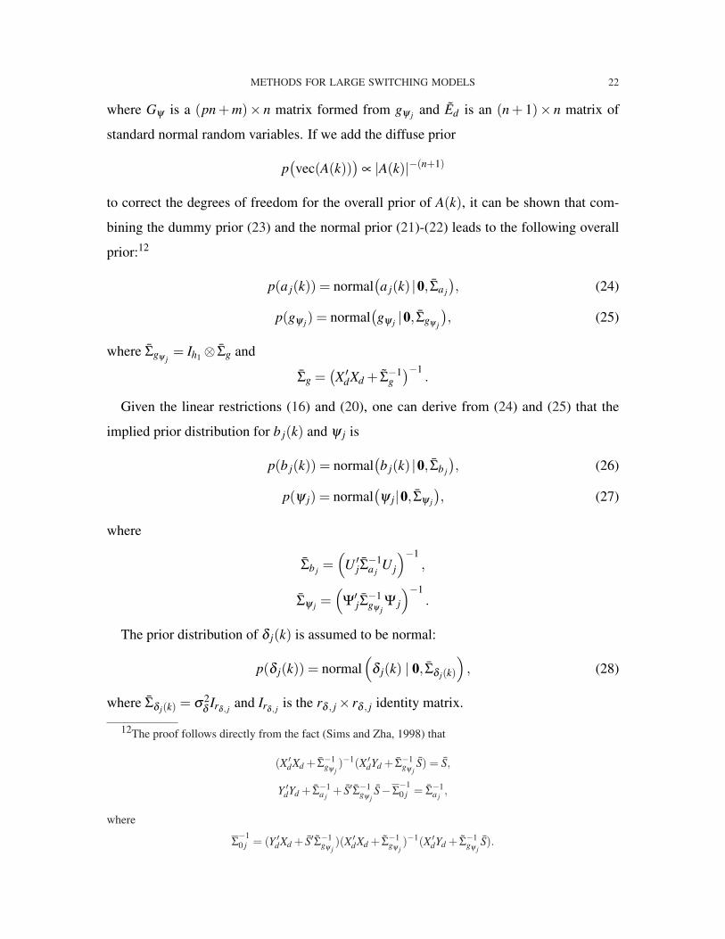
METHODS FOR LARGE SWITCHING MODELS 22
where Gψ is a (pn + m)× n matrix formed from gψ j and Ed is an (n + 1)× n matrix of
standard normal random variables. If we add the diffuse prior
p(vec(A(k))
)∝ |A(k)|−(n+1)
to correct the degrees of freedom for the overall prior of A(k), it can be shown that com-
bining the dummy prior (23) and the normal prior (21)-(22) leads to the following overall
prior:12
p(a j(k)) = normal(a j(k) |0, Σa j
), (24)
p(gψ j) = normal(gψ j |0, Σgψ j
), (25)
where Σgψ j= Ih1 ⊗ Σg and
Σg =(X ′dXd + Σ−1
g)−1
.
Given the linear restrictions (16) and (20), one can derive from (24) and (25) that the
implied prior distribution for b j(k) and ψ j is
p(b j(k)) = normal(b j(k) |0, Σb j
), (26)
p(ψ j) = normal(ψ j|0, Σψ j
), (27)
where
Σb j =(
U ′jΣ−1a j
U j
)−1,
Σψ j =(
Ψ′jΣ−1gψ j
Ψ j
)−1.
The prior distribution of δ j(k) is assumed to be normal:
p(δ j(k)) = normal(
δ j(k) | 0, Σδ j(k)
), (28)
where Σδ j(k) = σ2δ Irδ , j and Irδ , j is the rδ , j× rδ , j identity matrix.
12The proof follows directly from the fact (Sims and Zha, 1998) that
(X ′dXd + Σ−1gψ j
)−1(X ′dYd + Σ−1gψ j
S) = S,
Y ′dYd + Σ−1a j
+ S′Σ−1gψ j
S−Σ−10 j = Σ−1
a j,
where
Σ−10 j = (Y ′dXd + S′Σ−1
gψ j)(X ′dXd + Σ−1
gψ j)−1(X ′dYd + Σ−1
gψ jS).
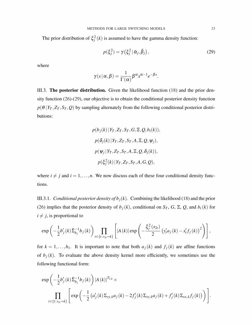
METHODS FOR LARGE SWITCHING MODELS 23
The prior distribution of ξ 2j (k) is assumed to have the gamma density function:
p(ξ 2j ) = γ
(ξ 2
j | α j, β j), (29)
where
γ (x |α,β ) =1
Γ(α)β αxα−1e−βx.
III.3. The posterior distribution. Given the likelihood function (18) and the prior den-
sity function (26)-(29), our objective is to obtain the conditional posterior density function
p(θ |YT ,ZT ,ST ,Q) by sampling alternately from the following conditional posterior distri-
butions:
p(b j(k) |YT ,ZT ,ST ,G,Ξ,Q,bi(k)),
p(δ j(k) |YT ,ZT ,ST ,A,Ξ,Q,ψ j),
p(ψ j |YT ,ZT ,ST ,A,Ξ,Q,δ j(k)),
p(ξ 2j (k) |YT ,ZT ,ST ,A,G,Q),
where i 6= j and i = 1, . . . ,n. We now discuss each of these four conditional density func-
tions.
III.3.1. Conditional posterior density of b j(k). Combining the likelihood (18) and the prior
(26) implies that the posterior density of b j (k), conditional on ST , G, Ξ, Q, and bi (k) for
i 6= j, is proportional to
exp(−1
2b′j (k) Σ−1
b jb j (k)
)∏
t∈t: s1t=k
[|A(k)|exp
(−ξ 2
j (s2t)2
(y′ta j (k)− x′t f j (k)
)2
)],
for k = 1, . . . ,h1. It is important to note that both a j (k) and f j (k) are affine functions
of b j (k). To evaluate the above density kernel more efficiently, we sometimes use the
following functional form:
exp(−1
2b′j (k) Σ−1
b jb j (k)
)|A(k)|T1,k×
∏t∈t: s1t=k
[exp
(−1
2(a′j (k)Σyy,ka j (k)−2 f ′j (k)Σxy,ka j (k)+ f ′j (k)Σxx,k f j (k)
))].
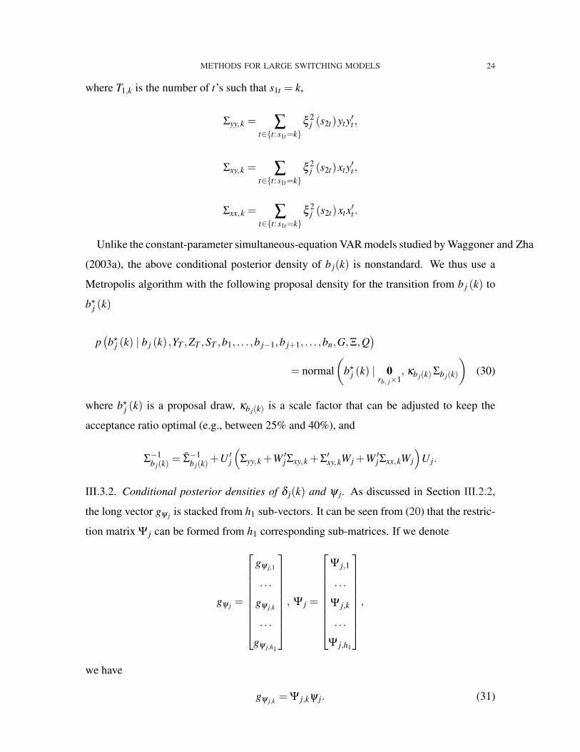
METHODS FOR LARGE SWITCHING MODELS 24
where T1,k is the number of t’s such that s1t = k,
Σyy,k = ∑t∈t: s1t=k
ξ 2j (s2t)yty′t ,
Σxy,k = ∑t∈t: s1t=k
ξ 2j (s2t)xty′t ,
Σxx,k = ∑t∈t: s1t=k
ξ 2j (s2t)xtx′t .
Unlike the constant-parameter simultaneous-equation VAR models studied by Waggoner and Zha
(2003a), the above conditional posterior density of b j(k) is nonstandard. We thus use a
Metropolis algorithm with the following proposal density for the transition from b j (k) to
b?j (k)
p(b?
j (k) | b j (k) ,YT ,ZT ,ST ,b1, . . . ,b j−1,b j+1, . . . ,bn,G,Ξ,Q)
= normal(
b?j (k) | 0
rb, j×1, κb j(k) Σb j(k)
)(30)
where b?j (k) is a proposal draw, κb j(k) is a scale factor that can be adjusted to keep the
acceptance ratio optimal (e.g., between 25% and 40%), and
Σ−1b j(k)
= Σ−1b j(k)
+U ′j
(Σyy,k +W ′
jΣxy,k +Σ′xy,kW j +W ′jΣxx,kWj
)U j.
III.3.2. Conditional posterior densities of δ j(k) and ψ j. As discussed in Section III.2.2,
the long vector gψ j is stacked from h1 sub-vectors. It can be seen from (20) that the restric-
tion matrix Ψ j can be formed from h1 corresponding sub-matrices. If we denote
gψ j =
gψ j,1
. . .
gψ j,k
. . .
gψ j,h1
, Ψ j =
Ψ j,1
. . .
Ψ j,k
. . .
Ψ j,h1
,
we have
gψ j,k = Ψ j,kψ j. (31)

METHODS FOR LARGE SWITCHING MODELS 25
From the conditional likelihood (18), the prior distribution (28), and the restriction (19),
one can obtain the posterior density kernel of δ j (k) conditional on ST , A, Ξ, Q, and ψ j as
h1
∏k=1
exp(−1
2δ j(k)′Σ−1
δ j(k)δ j(k)
)×
∏t∈t: s1t=k
exp
(−ξ 2
j (s2t)2
((y′t + x′tW j
)U jb j (k)− x′tV jdiag
(gψ j,k
)(∆ jδ j(k)+ δ j
))2)
.
Rearranging the terms in the above equation leads to
p(δ j (k) | YT ,ZT ,ST ,A,Ξ,Q,ψ j
)= normal
(δ j (k) | µδ j(k), Σδ j(k)
), (32)
where
Σ−1δ j(k)
= ∆′jdiag(gψ j,k
)V ′
jΣxx,kV jdiag(gψ j,k
)∆ j,
Σ−1δ j(k)
= Σ−1δ j(k)
+ Σ−1δ j(k)
,
µδ j(k) = ∆′jdiag(gψ j,k
)V ′
j
[∑
t∈t: s1t=kξ 2
j (s2t)xt(y′t + x′tWj
)]
U jb j (k) ,
µδ j(k) = Σδ j(k)
(µδ j(k)− Σ−1
δ j(k)δ j
).
Similarly, from the conditional likelihood (18), the prior distribution (27), and the re-
striction (31), we obtain the posterior density kernel of ψ j conditional on ST , A, Ξ, Q, and
δ j as
h1
∏k=1
exp(−1
2ψ ′
jΣ−1ψ j
ψ j
)×
∏t∈t: s1t=k
exp
(−ξ 2
j (s2t)2
((y′t + x′tWj
)U jb j (k)− x′tV jdiag
(gδ j(k)
)Ψ j,kψ j
)2)
.
Rearranging the terms in the above equation gives
p(ψ j | YT ,ZT ,ST ,A,Ξ,Q,δ j
)= normal
(δ j (k) | µψ j , Σψ j
), (33)

METHODS FOR LARGE SWITCHING MODELS 26
where
Σ−1ψ j
=h1
∑k=1
Ψ′j,kdiag
(gδ j(k)
)V ′
jΣxx,kV jdiag(
gδ j(k)
)Ψ j,k,
Σ−1ψ j
= Σ−1ψ j
+ Σ−1ψ j
,
µψ j =h1
∑k=1
Ψ′j,kdiag
(gδ j(k)
)V ′
j
[∑
t∈t: s1t=kξ 2
j (s2t)xt(y′t + x′tWj
)]
U jb j (k) ,
µψ j = Σψ j µψ j .
III.3.3. Conditional posterior density of ξ 2j (k). Let T2,k be the number of elements in t :
s2t = k for k = 1, . . . ,h2. It follows that
p(ξ 2
j (k) | YT ,ZT ,ST ,A,G,Q)
= γ(
ξ 2j (k) | α j (k) , β j (k)
), (34)
where
α j (k) = α j +T2,k
2,
β j (k) = β j +12 ∑
t∈t: s2t=k
(y′ta j (s1t)− x′t f j (s1t)
)2.
III.4. Other types of Markov processes. The previous analysis can be easily extended
to other types of Markov processes. If we wish to synchronize the two state variables s1t
and s2t into one state variable st , we simply need to replace these two independent state
variables by this one common state variable st in the likelihood function. If we wish to
have an independent Markov process for the coefficients in each equation, s1t becomes a
composite state variable consisting of s j,1t for j = 1, . . . ,n. In this case, we simply replace
s1t by s j,1t for the time-varying coefficients in equation j in the likelihood function.
III.5. Normalization. To obtain the accurate posterior distributions of functions of θ (such
as long run responses, historical decompositions, and impulse responses), one must normal-
ize signs of structural equations; otherwise, the posterior distributions will be symmetric
with multiple modes, making statistical inferences of interest meaningless. Such normal-
ization is also essential to achieving efficiency in evaluating the marginal data density for
model comparison. We choose the Waggoner and Zha (2003b) normalization rule to de-
termine the signs of columns of A(k) and F(k) for any given k ∈ 1, . . . ,h. Since our
original prior is un-normalized and symmetric around the origin, this prior density must be
METHODS FOR LARGE SWITCHING MODELS 27
multiplied by 2n when the marginal data density is estimated with MCMC draws that are
normalized by the rule proposed by Waggoner and Zha (2003b).
Scale normalization on δ j(k1) and ξ j(k2) imposes the restrictions δ j(k1) = 1rδ , j×1 and
ξ j(k2) = 1 for j ∈ 1, . . . ,n, k1 ∈ 1, . . . ,h1, and k2 ∈ 1, . . . ,h2, where the notation
1rδ , j×1 denotes the rδ , j × 1 vector of 1’s. One could use other normalization rules (e.g.,
restricting each set of time-varying parameters on the unit circle). The marginal data den-
sity, however, is invariant to scale normalization, as long as the Jacobian transformation is
properly taken into account.
We do not perform any permutation of state-dependent parameters in our MCMC algo-
rithm. For each posterior draw of the parameters, the h! permutations of these parameters
give the same posterior density; thus we follow Geweke (2006) and store the h! copies in
our MCMC runs conceptually but not literally . In principle, one could normalize the la-
belling of states as suggested by Hamilton, Waggoner, and Zha (2004) or by Sims and Zha
(2006). For the same reason as outlined by Geweke (2006), this labelling does not affect
the value of the marginal data density.
IV. BLOCKWISE OPTIMIZATION ALGORITHM
In spite of the complexity inherent in the multiple-equation models considered in this
paper, it is essential to obtain the estimate of θ at the peak of the posterior distribution (7).
The posterior estimate or the maximum likelihood estimate, serving as a starting point for
our MCMC algorithm, ensures that an unreasonably long sequence of posterior draws do
not get stuck in the low probability region. Used as a reference point in normalization,
moreover, it helps avoid distorting the statistical inferences likely to be produced by in-
appropriate normalization. And the likelihood value conditional on the posterior estimate
helps detect obvious errors in computing marginal data densities for posterior odds ratios.
Hamilton (1994) proposes an expectation-maximizing (EM) algorithm for a simple Markov-
switching model. For multivariate dynamic models, however, the expectation step in gen-
eral has no analytical form. Chib (1996) proposes a Monte Carlo EM (MCEM) algorithm
in which the evaluation of the E-step of the EM algorithm is approximated by Monte Carlo
simulations from the posterior distribution.

METHODS FOR LARGE SWITCHING MODELS 28
As shown in Sims and Zha (2006), these MC simulations can be very expensive compu-
tationally. When the number of parameters is small, one may obtain the posterior estimate
of θ by simply finding the value of θ that maximizes the posterior density p(θ ,Q | YT ,ZT )
given by (7). Sims (2001) uses this approach for his single-equation model. But for a sys-
tem of multivariate dynamic equations, the number of model parameters can be too large
for a straight maximization routine to be reliable.
In this paper, we propose a different algorithm. We use the Gibbs-sampling idea to break
the parameters θ ,Q into two blocks of parameters θ and Q. In the multivariate dynamic
models considered in this paper, we break the block of parameters θ further into three sub-
blocks, one containing b j(k) for k = 1, . . . ,h1, one containing g j(k) for k = 1, . . . ,h1, and
third sub-block containing ξ 2j (k) for k = 1, . . . ,h2. Given an initial guess of the values of
the parameters, one can use the standard hill-climbing optimization routine (e.g., the Quasi-
Newton BFGS algorithm) to find the values of each block of parameters that maximizes
the posterior density while holding other blocks of parameters fixed at the previous values.
Iterate this algorithm across blocks until it converges. For each iteration, we also employ a
constrained optimization method to check whether there are boundary solutions associated
with Q or any other model parameters.
V. NEW IMPLEMENTATION OF THE MHM METHOD
For many empirical models, the modified harmonic mean (MHM) method of Gelfand and Dey
(1994) is a widely used method to compute the marginal data density. In this section we
discuss the potential problem with this method when the posterior distribution is very non-
Gaussian and propose a new way of implementing the MHM method to remedy this prob-
lem. For notational clarity, we restrict ourselves to the constant-parameter case, treat θ as
a collection of all the free parameters in the model, and omit the exogenous variables ZT .
At the end of this section, we discuss how to handle the Markov-switching models.
We begin by denoting the likelihood function by p(YT | θ) and the prior density be p(θ),
both of which must have proper probability densities instead of their kernels. Given these
two objects, the marginal data density is defined as
p(YT ) =∫
p(YT | θ)p(θ)dθ . (35)

METHODS FOR LARGE SWITCHING MODELS 29
The MHM method used to approximate (35) numerically is based on a theorem that
states
p(YT )−1 =∫
Θ
h(θ)p(YT | θ)p(θ)
p(θ | YT )dθ , (36)
where Θ is the support of the posterior probability density and h(θ), often called a weight-
ing function, is any probability density whose support is contained in Θ. Denote
m(θ) =h(θ)
p(YT | θ)p(θ).
A numerical evaluation of the integral on the right hand side of (36) can be accomplished
in principle through the Monte Carlo (MC) integration
p(YT )−1 =1N
N
∑i=1
m(θ (i)), (37)
where θ (i) is the ith draw of θ from the posterior distribution p(θ |YT ). If m(θ) is bounded
above, the rate of convergence from this MC approximation is likely to be practical.
Geweke (1999) proposes an implementation with h(·) constructed from the posterior
simulator. The sample mean θ and sample covariance matrix Ω can be calculated from
draws of θ from the posterior simulator. The weighting function is chosen to be a trun-
cated multivariate Gaussian density with mean θ and covariance Ω. The Gaussian density
is truncated to ensure that the support of the weighting function is contained in the sup-
port of posterior. Our experience suggests that this method works well for many existing
DSGE and VAR models with no time variation on the parameters. When one allows time
variation in the model’s parameters, the posterior density tends to be non-Gaussian. The
non-Gaussian phenomenon is manifested in three aspects. First, the posterior density may
be quite small at the sample mean, especially when the posterior density has multiple peaks.
Second, a truncated Gaussian density function may be a poor local approximation to the
posterior density. Third, as one can see from (8), the likelihood tends to be zero in the
interior points of the domain Θ.
To deal with these potential problems, we propose a more general class of distributions
than the Gaussian family, center and scale these distributions differently, and truncate them
in a more sophisticated manner. We begin with the easiest task, which involves the center-
ing and scaling. Instead of centering the weight pdf at the sample mean, we center at the
METHODS FOR LARGE SWITCHING MODELS 30
posterior mode θ and instead of scaling by the sample covariance matrix, we use
Ω =1N
N
∑i=1
(θ (i)− θ
)(θ (i)− θ
)′
where θ (i) denotes the ith draw from the posterior simulator and N is the sample size. Com-
puting the posterior mode is typically more expensive than computing the sample mean (see
Section IV), but it greatly improves efficiency of the MHM method. Instead of the Gaussian
family of distributions, we use elliptical distributions. An elliptical distribution centered at
θ and scaled by S =√
Ω has a density of the form
g(θ) =Γ(k/2)
2πk/2∣∣det
(S)∣∣
f (r)rk−1
where k is the dimension of θ , r =√(
θ − θ)′ Ω−1
(θ − θ
)and f is any one-dimensional
density defined on the positive reals. We note that the Gaussian is a special case in the
family of elliptical distributions. Since we know how to sample from the one dimensional
density f , making draws for an elliptical distribution is straightforward. Simply draw x
from a k-dimensional standard Gaussian distribution and r from the density f , and define
θ =r‖x‖ Sx+ θ .
The one-dimensional density f is chosen in the following way. For each draw θ (i) from
the posterior, let
r(i) =√(
θ (i)− θ)′ Ω−1
(θ (i)− θ
)
From these simulated r(i), we can easily form an estimate of their cumulative density func-
tion. The density f should be chosen so that its cumulative density closely matches the
estimated one. There are many ways to accomplish this task. For instance, f could be cho-
sen to be a step function such that the cumulative density is piecewise-linear approximation
of the estimated cumulative density. We chose a somewhat simpler technique. The density
f has support on [a,b] and is defined by
f (r) =vrv−1
bv−av
The hyperparameters a, b, and v are chosen as follows. Let c1, c10, and c90 be chosen
so that one percent of the r(i) are less than c1, ten percent of the r(i) are less than c10, and
ninety percent of the r(i) are less than c90. Denote the density function f (r) with a = 0 by

METHODS FOR LARGE SWITCHING MODELS 31
f0(r). The values of b and v are so chosen that the probability of r < c10 from f0 is 0.1 and
the probability of r < c90 from f0 is 0.9. These choices translate into
v =log(1/9)
log(c10/c90), b =
c90
0.91/v. (38)
For the reasons elaborated below, we set the value of a to c1. With the nonzero value of a
and the values of v and b specified in (38), one should note that the probability of r < cp
from f will not be exactly p, where p = 0.1 or p = 0.9.
We now turn to the method we use to truncate the elliptical distribution g. Let U be a
positive number and ΘU be the region defined by
ΘU = θ : m(θ) < U .
The weighting function h is chosen to be an elliptical density function truncated so that its
support is ΘU . If qU is the probability that draws from the elliptical distribution lies in ΘU ,
then h is given by
h(θ) =χΘU (θ)
qUg(θ) ,
where χA(θ) is an indicator function that returns one if θ falls in the set A and zero oth-
erwise. The value of qU can be estimated from random draws from the elliptical density
g. Since we can take i.i.d. draws from an elliptical distribution, the estimate of qU has a
binomial distribution and its accuracy can be readily obtained. The lower the truncation
value of U is, the larger the effective sample size of a sequence of MCMC draws is, but the
less acceptable the value of qU becomes. Therefore, there is a balance between having a
low value of U and having a reasonable estimate of qU .
Because we chose a nonzero value of a for f (r), the weight function h(θ) is effectively
bounded above. Thus, the upper bound truncation on m(θ) can be easily implemented by
a lower bound truncation on the posterior density kernel itself. Specifically, Let L be a
positive number and ΘL be the region defined by
ΘL = θ : p(YT | θ)p(θ) > L .
The weighting function h is chosen to be a truncated elliptical density such that its support
is ΘL. If qL is the probability that random draws from the elliptical distribution lies in ΘL,
then h is given by
h(θ) =χΘL (θ)
qLg(θ) .

METHODS FOR LARGE SWITCHING MODELS 32
Our computational experience tells us that a good choice of L is a value such that 90% of
draws from the posterior distribution lie in ΘL.
The new MHM method developed here is computationally more demanding than the
standard MHM implementation, but it avoids the potential problems associated with ill-
behaved patters of posterior draws of m(θ) when a Gaussian approximation to the posterior
distribution is poor. Denote the kernel of the posterior probability density by
k(θ |YT ) = p(YT | θ)p(θ).
The procedure for implementing our new MHM method is as follows.
(1) Simulate a sequence of posterior draws θ (i) and record the minimum and maximum
values of k(θ |YT ), denoted by kmin and kmax respectively. Let kmin < L < kmax.
(2) Simulate random draws of θ from g(θ) and compute the proportion of these draws
that belong to ΘL. This proportion, denoted by qL, is the estimate of qL. Note that
qL has a binomial distribution and depends on the number of MCMC draws and the
sample simulated from h(). If qL < 1.0e− 06, this estimate is unreliable because
three or four standard deviations will include the value zero. As a rule of thumb,
we keep qL ≥ 1.0e−04.
(3) For each value of L, estimate the marginal data density according to (37).
This procedure can also be implemented by selecting a good value of the upper bound U .
Denote the minimum and maximum values of m(θ) sampled from the posterior distribution
by mmin and mmax. For each value of mmin < U < mmax, compute an estimate of qU and
then obtain an estimate of the marginal data density accordingly.
We have thus far discussed our new MHM procedure based on the constant-parameter
case. For the Markov-switching models, the only difference is the treatment of the tran-
sition matrix Q in which w j for j = 1, . . . ,h is a vector of free parameters as discussed in
Section II.4. The transition matrix parameters w j’s are treated separately from θ and we
use a Dirichlet density instead of a truncated power density as the weighting function for
w j.

METHODS FOR LARGE SWITCHING MODELS 33
VI. APPLICATION
In this section we apply our method developed in the previous sections to a regime-
switching three-variable VAR model with five lags. The three variables are those commonly
used by recent DSGE models: log GDP (xt), GDP-deflator inflation (πt), and the federal
funds rate (Rt). The data are quarterly from 1959:I to 2005:IV. Recent debate on changes
in monetary policy has focused on whether the coefficients in the policy equation have
changed or the variance sizes for structural shocks have changed. Using the notation in
Section III.1, we let
yt =[xt πt Rt
]′.
Following the identification of Christiano, Eichenbaum, and Evans (2005), we consider the
upper triangular matrix A(st) where the last equation is the interest rate equation. We study
a large number of models and compare their fits to the data. The types of models are
described as follows
#v: Each equation is of Case II with # states under one common Markov process. We
call this type of model “variance-only.”
#vm: Each equation is of Case III with # states under one common Markov process.
We call this type of model “all-change” (i.e., both variances and means changing).
#vRm: The interest rate (R) equation (i.e., the third equation in our application) is of
Case III and the other two equations are of Case II with # states under one common
Markov process. We call this type of model “policy-change” (i.e., both variances
and coefficients in the policy equation changing).
#1v#2m: Each equation is of Case III, with #1 states under one Markov process for
a j(s1t) and f j(s1t) and with #2 states under the other independent Markov pro-
cess for ξ j(s2t), where j = 1, . . . ,n. We call this type of model “variance-with-all-
change.”
#1v#2Rm: The interest rate equation is of Case III and the other equations are of
Case II, with #1 states under one Markov process for a j(s1t) and f j(s1t) and with #2
states under the other independent Markov process for ξ j(s2t), where j = 1, . . . ,n.
We call this type of model “variance-with-policy-change.”

METHODS FOR LARGE SWITCHING MODELS 34
For all these quarterly models, the tightness values for the BVAR reference prior are, in
the notation of Sims and Zha (1998), λ0 = 1.0,λ1 = 1.0,λ2 = 1.0,λ3 = 1.2,λ4 = 0.1,µ5 =
1.0, and µ6 = 1.0. These hyperparameter values determine the prior covariance matrices
Σb j and Σψ j . For other prior settings, we follow Sims and Zha (2006) and set σδ = 50, α j =
1.0, and β j = 1.0. For the prior distribution of the transition probability q j as discussed in
Section II.4, we first begin with the case where q j is unrestricted, as this case is commonly
considered in the literature. We set αi, j = 1 for i 6= j and
α j, j =p j,dur(h−1)
1− p j,dur, (39)
where p j,dur = Eq j, j is the expected value of the probability of staying in the same state
(here state j). This prior setting, differing from that of Sims and Zha (2006), allows the
possibility that the posterior estimate of q j, j may be one (i.e., allowing the jth state to be
irreversible). For our quarterly data, we set p j,dur = 0.85, implying a prior belief that the
average duration of staying in the same state is between 6 and 7 quarters. For the four-state
case, it follows from (39) that
α j, j = 17, αi, j = 1 for i 6= j. (40)
In our application, we restrict the transition matrix in the pattern of (2) when the number
of states for a given Markov process is greater than two. Thus, in the case of four states,
the transition matrix is restricted as
Q =
π1 (1−π2)/2 0 0
1−π1 π2 (1−π3)/2 0
0 (1−π2)/2 π3 1−π4
0 0 (1−π3)/2 π4
. (41)
Take as an example the first two columns of Q in the case of (41). Expressing the restric-
tions on q1 and q2 in the form of (1), we have
q1,1 = w1,1, q2,1 = w2,1, q3,1 = 0, q4,1 = 0,
q2,2 = w2,2, q1,2 =12
w1,2, q3,2 =12
w1,2, q4,2 = 0.

METHODS FOR LARGE SWITCHING MODELS 35
If we take as given the values of αi, j specified in (39) (as supplied by a user who is used to
working on an unrestricted transition matrix) and transform them to βi, j as
βi, j = 1+ ∑(r,s): Mr, j(s,i)>0
(αr,s−1) ,
we have
β1,1 = α1,1, β2,1 = α2,1 = 1,
β2,2 = α2,2, β1,2 = α1,2 = 1.
According to (4), we have
Ew1,1 =β1,1
β1,1 +β2,1, Ew2,1 =
β2,1
β1,1 +β2,1,
Ew2,2 =β2,2
β2,2 +β1,2, Ew1,2 =
β1,2
β2,2 +β1,2.
With the values specified in (40), we have Eq j, j = Ew j, j = 0.94, implying a prior belief that
the average duration of staying in the same state is about 17 quarters, much longer than the
prior belief when Q is unrestricted. Although this is a prior we use for our application, we
recommend that in future research one should specify the prior on wi, j directly to maintain
the same prior belief on the average duration whether one works on an unrestricted or
restricted transition matrix.
Using the blockwise optimization algorithm described in Section IV, we obtain the pos-
terior estimates of the model parameters.13 With this estimate or any random value near
the neighborhood of this estimate as a starting point, we simulate a sequence of 20 million
MCMC draws to compute the marginal data density using the new method described in
Section V.14 For the case of 3 states, the restricted transition matrix takes the form of (2).
For the case of 4 states,
Table 1 reports log values of marginal data densities for nine different models. The
MDDs are not sensitive to the cutoff value L for our new MHM method. In the table, we
report only one value and the corresponding qL. For each sequence of MCMC draws, we
use the software R to compute an effective sample size (ESS) (i.e., the sample size adjusted
13For our C program, this algorithm takes less than 1 minute while the EM algorithm takes about 9 hours
on a Pentium-4 personal desktop computer.14It takes about 20 minutes to simulate one million MCMC draws.

METHODS FOR LARGE SWITCHING MODELS 36
for serial correlation of MCMC draws) according to Plummer, Best, Cowles, and Vines
(2005). For all the models studied in Table 1, the computed ESSs are near one million.15
Based on the ESS, thus, the numerical standard error on the estimated MDD is trivially
small. On the similar magnitude, we obtain very small numerical standard errors based on
the procedure of Newey and West (1987).
It is known, however, that these measures tend to deliver much smaller numerical stan-
dard errors than the actual ones. We propose a different measure by breaking a sequence of
20 million MCMC draws into 10 successive blocks with each block having 2 million draws.
For each block, we compute log value of the inverse of the estimated mean of m(θ) (by a
proper scaling to avoid an overflow in computation). The standard error of log MDD is then
computed according to the differences of log MDD across blocks and reported in Table 1.
As we can see, the standard error is much smaller for the 2-state variance-only model than
that for the 4-state variance-only model. In general, the standard error increases with the
degree of time variation. Figures 1 and 2 plot the values of log MDD across blocks for the
2-state and 3-state variance-only models. As can be seen, the estimated log MDD is quite
stable across blocks for the 2-state case where a Gaussian approximation is likely to be
good. For the 3-state variance-only model, however, we begin to see noticeable differences
across blocks.
The best-fit model is 3-state or 4-state variance-only model, which seems to dominate all
other models by taking into account the standard error of the estimated log MDD. Among
the models with changing coefficients, the 3v2Rm variance-with-policy-change model is
the best, which does not improve upon the 3-state variance-only model. The conclusion
that the variance-only model dominates remains if the Schwarz criterion is applied to the
posterior kernel.
To examine whether there exists any bias from our procedure in favor of variance-only
models or models with independent Markov processes, we simulate a series of 2000 data
points from the 2vRm model where the coefficients in the third equation switch between 2
states and the Markov process is the same for both coefficients and shock variances. We
apply our procedure to this artificial data set. The 2vRm model has the best fit with the
15Because of some memory management problems associated with the program R, the ESSs are estimated
on the smaller sample thinned by every twenty MCMC draws.

METHODS FOR LARGE SWITCHING MODELS 37
estimated log MDD being 19763.6. The second-best models are 3v2Rm with log MDD
being 19754.49 and 2v3Rm with log MDD being 19753.54. The other models have even
lower values of log MDD.
Our exercises point to the fact that accurate calculation of the MDD is an extremely
challenging task and give reasons why our method is useful when the posterior distribution
is non-Gaussian.
VII. CONCLUSION
We have developed methods of inference for a class of multiple-equation Markov-switching
models with restricted transition matrices. The methods apply to both structural and un-
restricted switching VARs. We have described a blockwise optimization algorithm that
proves to be much more efficient in these models than the EM algorithm that has been
widely applied to similar models. Our variant on the MHM method deals explicitly with
the problem of zero likelihood in the interior points of the parameter space. This problem
makes many of the usual estimates of the accuracy of results from MCMC simulations un-
reliable, and we suspect that the problem may be present and unrecognized in some of the
recent macroeconomic literature that reports posterior odds ratios on models.
We have proposed a new weighting function used by the MHM method, which is key to
obtaining reasonable estimates of marginal data densities in our exercises. This weighting
function is likely to be of general use, as in model comparison one often needs a reasonable
approximation of the posterior density whose distribution may be very non-Gaussian.
We hope the various ideas we have presented make possible wider use of this class of
models, since it represents one convenient approach to accounting for a salient fact about
economic time series — their volatilities, and occasionally their dynamic responses, change
over time.

METHODS FOR LARGE SWITCHING MODELS 38
TABLE 1. Marginal data densities by new MHM method
2v 2vm 2vRm 2v2m 2v2Rm
log(MDD) 1821.70 1831.72 1833.41 1857.80 1837.61
s.d. of log(MDD) 0.051 0.43 0.042 0.045 0.034
log(L) 1689.68 1647.12 1699.42 1640.25 1703.42
qL 0.381 1.6e-5 2.0e-3 1.72e-4 3.06e-4
2v3Rm 3v 3v2Rm 4v
log(MDD) 1839.47 1865.70 1863.04 1867.96
s.d. of log(MDD) 0.35 0.446 0.11 0.13
log(L) 1664.24 1719.14 1691.35 1717.53
qL 8.0e-6 5.77e-5 2.2e-5 5.1e-5
1 2 3 4 5 6 7 8 9 101821.6
1821.62
1821.64
1821.66
1821.68
1821.7
1821.72
1821.74
1821.76
1821.78
1821.8
log
MD
D
blocks
FIGURE 1. The 2-state variance-only (2v) model.

METHODS FOR LARGE SWITCHING MODELS 39
1 2 3 4 5 6 7 8 9 101865.2
1865.4
1865.6
1865.8
1866
1866.2
1866.4
1866.6
1866.8
1867lo
g M
DD
blocks
FIGURE 2. The 3 variance-only (3v) model.

METHODS FOR LARGE SWITCHING MODELS 40
APPENDIX A. COMPUTING U j , V j , AND Wj
We assume that a j and f j satisfy linear restrictions of the form
Q j
a j
f j
= 0
where Q j is a (n+ k)×(n+ k) with k = np+m. The matrix Q j will not be of full rank. We
show that there exist a n× q j matrix U j with orthogonal columns, a (pn+m)× r j matrix
V j with orthogonal columns, and a such that (pn+m)× n matrix W j with W ′jV j = 0 such
that
a j (k) = U jb j (k)
f j (k) = V jg j (k)−W jU jb j (k)
To prove this we rely on the following result:
Proposition 5. Given any r× s matrix X with r ≥ s, there exist an invertiable r× r matrix
Y and a s× s orthogonal matrix[
Z Z]
where Z is a s× q matrix and Z is a s× (s−q)
such that
Y−1X =
Z′
0
Proof. This follows directly from the singular value decomposition of X . Let X = UDV ′
where U is an r× r orthogonal matrix, V is a s× s orthogonal matrix, and D is a r× s
diagonal matrix where the first s−q diagonal elements are non-zero and the last q diagonal
elements are zero. The first s−q columns of V will be Z, the last q columns of V will be
Z, and Y = UE where E is the r× r diagonal matrix whose first s− q diagonal elements
are the first s− q diagonal elements of D, and the last r− (s−q) diagonal elements are
one. ¤
Applying the above propostion to the last k columns of Q j, there exists a (n+ k)×(n+ k)
invertiable matrix Y1 and a k×k orthogonal matrix[
V j V j
]where V j is k×(
k− r j)
and
V j is k× r j such that
Y−11 Q j =
W j V ′
j
U j 0
METHODS FOR LARGE SWITCHING MODELS 41
Now applying the above proposition to the(n+ r j
)×n matrix U j, there exists a(n+ r j
)×(n+ r j
)invertiable matrix Y2 and a n× n orthogonal matrix
[U j U j
]where U j is n×
(n−q j
)and U j is n×q j such that
Ik−r j 0
0 Y−12
Y−1
1 Q j =
Wj V ′j
U ′j 0
0 0
Thus a j and f j satisfy the restrictions if and only if W j V ′
j
U ′j 0
a j
f j
= 0.
Since both V ′jV j and U ′
jU j are equal to a identity matrix, writing a j = U jb j + U jc j and
f j = V jg j+ V jh j gives W j V ′
j
U ′j 0
a j
f j
=
WjU jb j +WjU jc j +h j
c j
.
This is zero if and only if c j = 0 and h j = −WjU jb j. If we define Wj = V jWj, then the
result follows.

METHODS FOR LARGE SWITCHING MODELS 42
REFERENCES
BEYER, A., AND R. E. FARMER (2004): “What We Don’t Know About the Monetary
Transmission Mechanism and Why We Don’t Know It,” Centre for Economic Policy
Research Discussion Paper No. 4811.
CANOVA, F., AND L. GAMBETTI (2004): “Structural Changes in the US Economy: Bad
Luck or Bad Policy,” Manuscript, Universitat Pompeu Fabra.
CHIB, S. (1996): “Calculating Posterior Distributions and Model Estimates in Markov
Mixture Models,” Journal of Econometrics, 75, 79–97.
CHRISTIANO, L., M. EICHENBAUM, AND C. EVANS (2005): “Nominal Rigidities and the
Dynamics Effects of a Shock to Monetary Policy,” Journal of Political Economy, 113,
1–45.
COGLEY, T., AND T. J. SARGENT (2002): “Evolving US Post-Wolrd War II Inflation
Dynamics,” NBER Macroeconomics Annual, 16, 331–373.
(2005): “Drifts and Volatilities: Monetary Policies and Outcomes in the Post
WWII U.S.,” Review of Economic Dynamics, 8, 262–302.
COOLEY, T. F., S. F. LEROY, AND N. RAYMON (1984): “Econometric policy evaluation:
Note,” The American Economic Review, 74, 467–470.
FARMER, R. E., D. F. WAGGONER, AND T. ZHA (2006): “Minimal State Variable Solu-
tions to Markov-Switching Rational Expectations Models,” Unpublished Manuscript.
GELFAND, A. E., AND D. K. DEY (1994): “Bayesian Model Choice: Asymptotics and
Exact Calculations,” Journal of the Royal Statistical Society (Series B), 56, 501–514.
GEWEKE, J. (1999): “Using Simulation Methods for Bayesian Econometric Models: In-
ference, Development, and Communication,” Econometric Reviews, 18(1), 1–73.
(2006): “Interpretation and Inference in Mixture Models: Simple MCMC Works,”
Manuscript, University of Iowa.
HAMILTON, J. D. (1989): “A New Approach to the Economic Analysis of Nonstationary
Time Series and the Business Cycle,” Econometrica, 57(2), 357–384.
(1994): Times Series Analsis. Princeton University Press, Princeton, NJ.
HAMILTON, J. D., D. F. WAGGONER, AND T. ZHA (2004): “Normalization in Economet-
rics,” Federal Reserve Bank of Atlanta Working Paper 2004-13.
METHODS FOR LARGE SWITCHING MODELS 43
KIM, C.-J., AND C. R. NELSON (1999): State-Space Models with Regime Switching. MIT
Press, London, England and Cambridge, Massachusetts.
LEEPER, E. M., AND T. ZHA (2003): “Modest Policy Interventions,” Journal of Monetary
Economics, 50(8), 1673–1700.
NEWEY, W. K., AND K. K. WEST (1987): “A Simple Positive Semi-Definite Het-
eroskedasticity and Autocorrelation Consistent Covariance Matrix,” Econometrica, 55,
703–708.
PLUMMER, M., N. BEST, K. COWLES, AND K. VINES (2005): “The coda Package,”
Version 0.10-2, November, [email protected].
PRIMICERI, G. (2005): “Time Varying Structural Vector Autoregressions and Monetary
Policy,” Review of Economic Studies, 72, 821–852.
ROBERTSON, J. C., AND E. W. TALLMAN (1999): “Vector Autoregressions: Forecasting
and Reality,” Federal Reserve Bank of Atlanta Economic Review, First Quarter, 4–18.
(2001): “Improving Federal-Funds Rate Forecasts in VAR Models Used for Policy
Analysis,” Journal of Business and Economic Statistics, 19(3), 324–330.
RUBIO-RAMÍREZ, J. F., D. F. WAGGONER, AND T. ZHA (2006): “Structural Vector Au-
toregressions: Theory and Application,” Manuscript, Duke University and Federal Re-
serve Bank of Atlanta.
SIMS, C. A. (1987): “A rational expectations framework for short-run policy analysis,” in
New approaches to monetary economics, ed. by W. A. Barnett, and K. J. Singleton, pp.
293–308. Cambridge University Press, Cambridge, England.
(1993): “A 9 Variable Probabilistic Macroeconomic Forecasting Model,” in Busi-
ness Cycles, Indicators, and Forecasting, ed. by J. H. Stock, and M. W. Watson, vol. 28
of NBER Studies in Business Cycles, pp. 179–214. University of Chicago Press.
(1999): “Drift and Breaks in Monetary Policy,” Manuscript, Princeton University.
(2001): “Stability and Instability in US Monetary Policy Behavior,” Manuscript,
Princeton University.
SIMS, C. A., AND T. ZHA (1998): “Bayesian Methods for Dynamic Multivariate Models,”
International Economic Review, 39(4), 949–968.
(2006): “Were There Regime Switches in US Monetary Policy?,” The American
Economic Review, 96, 54–81.

METHODS FOR LARGE SWITCHING MODELS 44
STOCK, J. H., AND M. W. WATSON (2003): “Has the Business Cycles Changed? Evidence
and Explanations,” Monetary Policy and Uncertainty: Adapting to a Changing Economy,
Federal Reserve Bank of Kansas City Symposium, Jackson Hole, Wyoming, August 28-
30.
WAGGONER, D. F., AND T. ZHA (2003a): “A Gibbs Sampler for Structural Vector Autore-
gressions,” Journal of Economic Dynamics and Control, 28(2), 349–366.
(2003b): “Likelihood Preserving Normalization in Multiple Equation Models,”
Journal of Econometrics, 114(2), 329–347.
ZHA, T. (In press): “Vector Autoregressions,” in The New Palgrave Dictionary of Econom-
ics, ed. by L. E. Blume, and S. Durlauf. Palgrave Macmillan.