Methods for Automatic Detection of Artifacts in Microelectrode Recordings

Eduard Baksteina,b,∗, Tomas Siegera,c, Jirı Wilda, Daniel Novaka, Jakub Schneidera,b, Pavel Vostateka, Dusan Urgosıkd,Robert Jechc

aDepartment of Cybernetics, Faculty of Electrical Engineering, Czech Technical University in Prague, Czech RepublicbNational Institute of Mental Health, Klecany, Czech Republic

cDepartment of Neurology and Center of Clinical Neuroscience, First Faculty of Medicine and General University Hospital, Charles University,Prague, Czech Republic

dDepartment of Stereotactic Neurosurgery and Radiosurgery, Na Homolce Hospital, Prague, Czech Republic

Abstract

Background: Extracellular microelectrode recording (MER) is a prominent technique for studies of extracellularsingle-unit neuronal activity. In order to achieve robust results in more complex analysis pipelines, it is necessary tohave high quality input data with a low amount of artifacts. We show that noise (mainly electromagnetic interferenceand motion artifacts) may affect more than 25% of the recording length in a clinical MER database.

New Method: We present several methods for automatic detection of noise in MER signals, based on i) unsuperviseddetection of stationary segments, ii) large peaks in the power spectral density, and iii) a classifier based on multipletime- and frequency-domain features. We evaluate the proposed methods on a manually annotated database of 5735ten-second MER signals from 58 Parkinson’s disease patients.

Comparison with Existing Methods: The existing methods for artifact detection in single-channel MER that havebeen rigorously tested, are based on unsupervised change-point detection. We show on an extensive real MER databasethat the presented techniques are better suited for the task of artifact identification and achieve much better results.

Results: The best-performing classifiers (bagging and decision tree) achieved artifact classification accuracy of up to89% on an unseen test set and outperformed the unsupervised techniques by 5-10%. This was close to the level ofagreement among raters using manual annotation (93.5%).

Conclusion: We conclude that the proposed methods are suitable for automatic MER denoising and may help in theefficient elimination of undesirable signal artifacts.

Keywords: microelectrode recordings, artifact detection, external noise, supervised classification

Cite as

Bakstein, E., Sieger, T., Wild, J., Novak, D., Schneider, J., Vostatek, P., . . . Jech, R. (2017). Methods for automaticdetection of artifacts in microelectrode recordings. Journal of Neuroscience Methods, 290, 39–51. https://doi.org/10.1016/j.jneumeth.2017.07.012

Note: This is the author’s version of the accepted article. The journal version is to be found at the publisher usingthe doi link above. Visit also http://neuro.felk.cvut.cz for supplementary matlab codes, sample data andinformation on our related research.

Highlights

• Artifacts are common in intra-operative micro electrode recordings (MER) - up to 25%.• We propose a set of classifiers for automatic artifact detection.• The methods are evaluated on a database of 5735 manually labeled MER signals.• The best-performing classifiers achieved up to 89% test-set accuracy.• Matlab source codes and sample data are available in the supplement.

Author’s version from August 1, 2017, distributed under

1. Introduction

Extracellular microelectrode recording (MER) usingelectrodes with a tip size around 1 µm [1] is a basic tech-nique for acquiring extracellular electric activity at thelevel of individual neurons (single-unit activity). Dueto the small electrode size and the low voltage of thesource signal, MER is susceptible to mechanical shiftsand electromagnetic interference, resulting in signal arti-facts [2]. While some components of the external noisecan be filtered easily (e.g. 50 Hz or 60 Hz mains noisefiltering using a notch or comb digital filter or sophisti-cated hardware design [3]) other may be more difficultto define and suppress.

In this study, we describe aspects of the most preva-lent artifacts, as observed on an MER database, obtainedfrom exploratory microelectrodes immediately beforeimplantation of permanent electrode for deep brain stim-ulation (DBS) and we propose a set of classifiers foridentifying them. As the DBS technique has been usedroutinely in movement disorder therapy for more thantwo decades [4] and MER is still used in the vast ma-jority of DBS centers worldwide [5], DBS surgery alsoserves as a prominent source of human sub-cortical neu-ronal data for scientific purposes. Irrespective of thevalue that DBS MER signals may have for the researchcommunity, it is clinical considerations that mostly deter-mine the procedure and put strain on the available timeand instrumentation. Sources of undesired artifacts inDBS surgery include electrical appliances in the oper-ating room, electrode vibration (after manual electrodeshifting or touches applied to the microdrive or stereo-tactic frame), and movement or speech of the patient.Artifacts are therefore commonly found in DBS MERdata, and we also illustrate this on data samples from 58Parkinson’s disease patients.

The presence of artifacts in an MER signal may havea dramatic impact on subsequent signal processing. Itsseverity will depend on the particular processing pipeline,and also on the character of the artifact. In the case of sin-gle or multi-unit analysis, a spike detection method andspike sorting methods are used to separate the activity ofneurons close to the electrode tip from the background ac-tivity (i.e. the summary activity of neurons further awayfrom the electrode [6, 7]). Widely-applied extracellularspike detection methods use amplitude distribution toestimate an appropriate value of the detection threshold[8, 9, 10], and are therefore sensitive to the background

∗Corresponding authorEmail address: eduard.bakstein@fel.cvut.cz (Eduard

Bakstein)

noise level [11], and also to artifacts. The impact of arti-facts on spike detection results may be mitigated to someextent by the use of a robust estimator of the neuronalbackground level [12] and subsequent removal of spikesof anomalous shape [9, 13]. However, external artifactsremain a significant source of undesirable noise in thewhole (mostly statistical) analysis pipeline, and they maylead to a loss of sensitivity or to noise in the resultingspike trains.

1.1. Existing artifact detection approaches

The prevailing approach for obtaining an artifact-free dataset in MER-based studies relies on manual in-spection and disposal of contaminated signal segments[14, 15]. However, this approach may be lengthy andmay still not provide optimal results, as some artifactscannot be identified solely from the time series plot, dueto their low projection to signal envelope. In such cases,other modalities, including spectrogram and audio play-back, are needed in order to identify all artifacts. Manyresearchers therefore use their own (semi) automaticmethods, ranging from simple amplitude thresholding[16], through statistical testing of the amplitude distribu-tion in short signal windows [17, 18], to sophisticatedamplitude and power spectral density (PSD) based sys-tems [19, 20, 21]. The detection thresholds are usuallyselected to match the investigator’s subjective evaluation,and the actual classification performance is not rigor-ously tested.

Two methods for identifying stationary MER seg-ments (i.e. segments consistent in a selected signal fea-ture) have been published in detail with a formal perfor-mance evaluation. The first of these methods is basedon the variance of the autocorrelation function [22, 23],while the other method is based on the variance of the sig-nal wavelet decomposition [24]. These methods, whilesuitable for detection of rapid changes in amplitude (aspresented on simulated data in the original publications),seem to be less appropriate for motion artifacts and forelectromagnetic interference [25], two of the most preva-lent noise types observed on our DBS MER database.

1.2. Proposed artifact detection method

As we showed in our previous paper [25], much betterdetection results than for the existing solutions can beachieved by a simple linear classifier based on the powerspectral density (PSD) of the signal. In this paper, weextend this approach by presenting an artifact detectionmodel based on multiple time domain and spectral fea-tures. We tested a range of models based on decisiontrees, support vector machines (SVM) and boosting, and

2

we evaluated their performance together with previouslypublished solutions on an extensive manually annotatedDBS MER database.

2. Methods

2.1. Data collection

All data used in this study were collected during elec-trophysiological exploration for deep brain stimulationsurgery at Na Homolce Hospital, Prague, Czech Repub-lic. All patients were implanted either unilaterally orbilaterally, using one to five microelectrodes in a cru-ciform configuration (the ”Ben-gun”), spaced at inter-vals of 2 mm around the central electrode. The signalswere recorded using the Leadpoint recording system(Medtronic, MN) at a sampling rate of 24 kHz, and wereband-pass filtered between 500-5000 Hz upon record-ing. The median recording length was 10 s, and signalsshorter than 5 s were discarded. The data recording waspart of an unaltered standard surgical procedure, withwhich all patients had agreed by signing the informedconsent.

All annotation, classification and data handling wasperformed in MATLAB (The MathWorks, Inc., Natick,Massachusetts, United States).

2.2. Manual artifact data annotation

The data annotation was based on visual and auditoryinspection of multi-channel signal time series. Addi-tionally, the annotator was provided with a spectrogramheatmap, showing short-time Fourier transform spectraon a parallel time scale with the time series. All datawere annotated in 1 s windows, as further experimentsshowed a very low level of agreement between raters ina scenario where the exact start and end of the artifactswas determined by each user. In cases where the dataincluded multiple channels from electrodes recorded si-multaneously, all channels were visualized in parallel foreasier identification of movement artifacts, often span-ning across multiple channels [26].

To achieve a high level of concordance, the team offive annotators (neurologists or engineers with long-termexperience with MER processing) underwent repetitiveannotation of a set of 20 multi-channel signals, and thediscrepancies between raters were discussed after eachof the three rounds. In the subsequent phase, the teamannotated the whole database of 1676 multi-channel sig-nals (i.e. about 330 signal sets per member), with a smallproportion of signals shared among the team. In the sub-sequent evaluation, the shared set of signals was used toevaluate the level of agreement among raters.

2.2.1. Observed artifactsFor the purposes of annotation, and also for further

analysis and evaluation, the observed artifacts weregrouped into the following clusters (cluster acronymsand the percentage of signal seconds containing a givenartifact on the cross-validation database are given inparenthesis)

• A mechanical movement artifact, manifested byshort-time, high-power signal peaks, usually spreadacross the whole frequency spectrum. (POW, 4.8%),see Fig. 1 A) and C).

• Low-frequency interference below the mains fre-quency (50 Hz), causing visible variation in thesignal offset or in the baseline (BASE, 7.6%)

• Electromagnetic interference at one or multiple sta-ble frequencies, well localized in a narrow band(s)in the frequency spectrum and stable over time(FREQ, 17.6%). The frequency of the observedlong-term interference often differed from the ex-pected odd harmonics of the mains frequency(50 Hz, 150 Hz, 250 Hz etc.), see Fig. 1 B).

• An ”irritated neuron”: spiking activity of very highand variable amplitude and firing rate (IRRIT, 0.3%)

• Other artifacts that cannot be assigned into any ofthe groups above. (OTHR, 0.2%)

Each second of the MER signal may contain one artifacttype, or several artifact types at the same time. A cleansignal (CLN, 74.6%) is defined as a signal with no arti-facts. Three examples of artifact-bearing MER signalscan be found in Figure 1. Detailed tabulation of the arti-fact percentage in our cross-validation and test datasetscan be found in Table A.1 in the Appendix. Twenty ex-ample MER signals with the different artifact types canbe found in the online supplementary material.

2.3. Automatic classification methodsDue to the relatively low level of agreement on the

exact artifact type among the annotators, all classifierswere designed only as two-class classifiers, trained todistinguish clean signals (CLN) from signals with allother artifact types.

2.3.1. Stationary segmentation methodsTwo stationary segmentation methods have been de-

scribed, by i) Falkenberg and Aboy et al. [22, 23], basedon variance of the signal autocorrelation function andii) by Guarnizo et al. [24], based on variance of the sig-nal wavelet decomposition. In these methods, the signal

3

0 500 1000 1500 2000−200

−100

0

100

200

signal A

0 500 1000 1500 20000

500

1000

1500

2000

0 500 1000 1500 2000−100

−50

0

50

100

signal B

time [ms]0 500 1000 1500 2000

0

500

1000

1500

2000

0 500 1000 1500 2000−40

−20

0

20

40

60

signal C

0 500 1000 1500 20000

500

1000

1500

2000

freq

uenc

y [H

z]am

plitu

de [a

.u.]

SPEC

TRO

GRA

M

MER

Figure 1: Two-second examples of the most commonly observed artifacts: a raw MER signal with artifact regions in light grey (top row, y-axisin arbitrary units), and the corresponding spectrogram (bottom row). Signal A) represents an intermittent mechanical artifact (POW), signal B)represents uninterrupted electromagnetic interference at ca 420, 840 and 1240 Hz (FREQ), and signal C) represents two minor mechanical artifacts(POW). The dark-grey segments in A) and C) represent a clean signal (CLN).

is first divided into short fixed-length segments. Subse-quently, the variance ratio of the statistics of neighboringsignal segments is computed, and is compared with amanually preset threshold. Points exceeding the thresh-old are marked as change points, and denote boundariesbetween stationary segments. Both methods focus solelyon signal segmentation and do not imply which of thestationary segments contains a clean signal (or artifacts).

In our previous work [25], we presented an extensionto these methods: instead of comparing the neighboringsegments only, the method computes the distance ma-trix between all possible segment pairs and searchesfor the largest available component, connected by asub-threshold path. Assuming higher stationarity inthe clean signal segments, rather than in the artifact-bearing segments, the largest component is then markedas a clean signal, while the remaining signal sectionsare marked as artifacts. For further technical details,the reader is referred to [25], or to Appendix B ofthis text. The extended methods are abbreviated be-low as COV (autocorrelation-based approach) and SWT(wavelet-based approach).

For the purposes of performance evaluation, we opti-mized three parameters of each algorithm: i) the segment

length (0.25, 0.33, 0.5 or 1 s), ii) the detection threshold,and iii) the number of segments within a one-second win-dow labeled by the classifier as an artifact, which wasnecessary for marking the whole second as an artifact(this last point was necessary since the manual annota-tion labels were available for one-second windows only).Implementation of the COV method is available in theonline supplementary material.

2.3.2. The maximum spectral difference methodA simple detection method, based on the power spec-

tral density of MER signals, was also presented in ourpaper [25]. The basic assumption is that the power spec-tral density (PSD) of a clean band-pass filtered MER sig-nal is smooth, unlike most signals with artifacts, whichcommonly contain high peaks and other disturbances.In the first step, a mean spectrum C of clean signalsegments is calculated from a set of N training signalsX = X1, X2, ..., XN with the corresponding artifact an-notation a = a1, a2, ..., aN, with ai equal to 1 for cleansignals and equal to 0 for signals with artifacts, accordingto:

C =1∑N

i=1 ai·

N∑i=1

a j P j, (1)

4

where P j is the normalized power spectral density (alsonorm. PSD) of signal segment X j of fixed length of 1s:signal PSD is computed using Welch’s method and isdivided by its sum. Therefore, the sum of all spectralbins in the resulting P spectrum is equal to one, and isthus independent of the total signal power. The length ofthe discrete Fourier spectrum was set to M = 2048, equalto the window length (Hamming type)1. The windowoverlap was set to 50%.

For an unseen signal segment with normalized spec-trum P j, the maximum absolute difference from themean spectrum of clean segments C can be calculatedby finding the maximum value over all M spectral bins:

d = maxm=1...M

| P j(m) − C(m) | (2)

The optimal detection threshold for d was set to thevalue that maximized performance (the J-statistic – seeEquation 3 below) on the training dataset. Once fixed,the threshold was used for classification. A clean spec-trum C, and also the spectrum for the three major artifacttypes, can be found in Figure 2. A Matlab implementa-tion of the method is available in the online supplemen-tary material. Throughout the performance comparisonbelow, all spectra for the spectral method (abbreviatedmaxAbsDiffPSD) were computed from one-second sig-nal segments.

0 500 1000 1500 2000 2500 30000

0.01

0.02

0.03

NPS

D [-

]

clean (CLN)

0 500 1000 1500 2000 2500 30000

0.01

0.02

0.03

large amplitude artif. (POW)

0 500 1000 1500 2000 2500 3000

frequency [Hz]

0

0.01

0.02

0.03

uctuating baseline (BASE)

0 500 1000 1500 2000 2500 30000

0.01

0.02

0.03

electromagnetic interference (FREQ)

p5% and p95%meanmean CLN

Figure 2: Normalized power spectral density for different artifacttypes, each computed from 1000 randomly selected signals from thecross-validation dataset. The mean value for each type of artifact (or-ange) with the 5th and 95th percentile for each spectral bin is comparedwith the normalized PSD (C) of clean signals (black).

1 See Appendix C for a discussion of spectrum length and the PSDestimation method.

2.3.3. Multi-feature classifiersIn addition to the simple detection methods mentioned

above, we have implemented a range of classificationmethods based on multiple features derived from the rawMER signal and its normalized power spectrum. Thefeatures were designed to describe the most prominentproperties of various artifact types, in comparison witha clean MER signal. After initial classification tests ona sample from the cross-validation database, misclassi-fied samples were identified, and were used to deviseadditional features (maxCorr and ksnorm). The initialtests were also used to specify feature properties – suchas the length of the Fast Fourier Transform (FFT), and toidentify suitable classifier parameter ranges for furthertesting.

For all features based on the frequency spectrum, thenormalized power spectral density was computed accord-ing to the definition in section 2.3.2 above, using Welch’smethod with FFT of length 2048 (equal to the windowlength - Hamming type) and 50% window overlap. Fea-tures were calculated from one-second signal segmentsto match the temporal resolution of the annotation. All19 features in the feature set are summarized in Table 1.

Due to the similarity in the definition of some fea-tures, high inter-feature correlation is to be expected –e.g. psdMaxStep and psdMax, due to the very sharpcharacter of the spectral peaks in signals with electro-magnetic interference, or sigP90 and sigP95, due to thesmooth character of the signal amplitude distributionin the lower percentiles. Therefore, all selected classi-fication methods have to perform some sort of featureselection, allowing for correlated features. The multi-feature classifiers that have been implemented include:

• The decision tree classifier, with limits on mini-mum parent node and leaf size, and different split-ting criteria.

• The Support Vector Machine (SVM) classifier,with a linear or radial-basis kernel using differentoptimization methods and kernel properties. TheSVM classifier was preceded by the feature selec-tion step – see the description below.

• Boosting classifiers, using various algorithms (Ad-aBoostM1, LogitBoost, GentleBoost, RobustBoost,Bagging) and varying the learning rate. The weaklearner that was used was a decision stump (boost-ing) or a decision tree (bagging).

All classifier parameters and the ranges across whichthey were optimized can be found in Table E.1. Anexhaustive search of all possible combinations of param-eters was performed for each classifier type.

5

The SVM classifier was preceded by a feature selec-tion step in order to reduce the number of features, andalso to reduce their redundancy. We used forward wrap-per feature selection with a discriminant analysis classi-fier. The algorithm starts with an empty feature set andadds a single feature that provides the best accuracy us-ing the selected classifier. Then, all possible sets of twofeatures, including the already selected feature and a can-didate feature from the remaining part of the feature setare tested. The best-performing two-feature set is fixed,and the process continues with three-feature sets andso on, until the stopping criterion (minimum improve-ment in classification accuracy) is achieved. The classi-fier used for feature selection was discriminant analysis(linear, quadratic or Mahalanobis distance-based), andwe used internal 5-fold crossvalidation to estimate out-of-sample performance. The classifier type used forfeature selection, as well as the value of the stoppingcriterion, was subject to parameter optimization, and allpossible combinations were tested (see Table E.1 in theAppendix).

2.4. Crossvalidation schemeIn order to evaluate the out-of-sample classifier perfor-

mance (i.e. performance on unseen data), we divided thetraining data from our database into two datasets: datafrom three DBS patients (6 MER trajectories, each con-sisting of 5 parallel micro-electrodes) were kept aside forfinal classifier testing as the test set, while the remain-der, denoted cross-validation (or CV) set, were usedfor feature evaluation, classifier training and parameteroptimization.

The main crossvalidation procedure was as follows:1. Ten-fold crossvalidation: The cross-validation

dataset was divided randomly into 10 subsets. Ineach iteration, all parameter combinations weretrained on 9 subsets and were validated on the re-maining subset. The confusion matrix on the vali-dation sample was stored for each combination ofparameter values and the process continued withthe next iteration. Data from individual patientswere kept together, never using data from the samepatient for training and for validation in one itera-tion.

2. Parameter optimization: Once the cross-validation was completed, the parameter set whichoptimized the validation performance of each clas-sifier type was selected.

3. Final classifier training: Each classifier wastrained on the whole cross-validation dataset, us-ing the optimal parameters obtained in the previousstep.

Table 1: Feature set overview

feature definition rationale

pow signal power in the en-tire window

higher overall powerin signal windowswith artifacts

powDiff maximum power dif-ference between adja-cent 0.05s signal seg-ments

power artifacts abruptin time

sigP90,sigP95,sigP99

raw signal amplitudepercentile (90th,95th,99th)

artifacts commonly in-clude peaks of verylarge amplitude

ksnorm value of the KSstatistic of the one-sample Kolmogorov-Smirnov normalitytest in the entirewindow

pronounced non-normality in signalswith artifacts

maxCorr maximum correlationcoefficient amongmultiple signalchannels in 0.05signal segments

mechanical artifactsoften spread acrosschannels and causehigh outlier values andthus high correlation

psdP75,psdP90,psdP95,psdP99

percentile of norm.PSD

artifacts localized inspectrum - high spec-tral peaks

psdMax,psdStd

maximum andstandard deviation ofnorm. PSD

global PSD descrip-tion

psdMaxStep maximum differencebetween adjacent binsof the norm. PSD

artifacts localized inspectrum - sharp spec-tral peaks

psdF100 maximum of the norm.PSD below 100 Hz

baseline artifacts ata well localized fre-quency

psdFreq maximum of the norm.PSD, divided by me-dian value below 5kHz

additional normaliza-tion of the norm. PSD

psdPow maximum of the norm.PSD in range 60-600Hz, divided by meannorm. PSD between 1and 3 kHz

power artifacts verycommon in this range

psdBase maximum of the norm.PSD in range 1-60Hz,divided by mean norm.PSD between 1 and 3kHz

baseline artifacts, nor-malized

maxAbsDiffPSD

maximum absolutedistance betweennorm. PSD andmean norm. PSD ofclean sample signalsegments

high artifact peaks inPSD

6

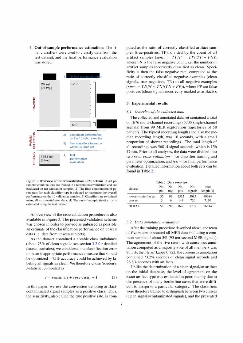
4. Out-of-sample performance estimation: The fi-nal classifiers were used to classify data from thetest dataset, and the final performance evaluationwas stored.

CV set(93 traj.)

TEST set(6 traj.)

TRAI

NIN

GTE

STIN

G

9/10

1/10

1) 10-fold crossvalidation

classifier training

performanceevaluation

PAR

AM.

SELE

CTI

ON 2) best mean performance

on the 10 valid. samples

3) final classifiers trained on whole CV data set

testperformanceevaluation

4)

Figure 3: Overview of the crossvalidation (CV) scheme 1) All pa-rameter combinations are trained in a tenfold crossvalidation and areevaluated on ten validation samples. 2) The final combination of pa-rameters for each classifier type is selected to maximize the overallperformance on the 10 validation samples. 3) Classifiers are re-trainedusing all cross-validation data. 4) The out-of-sample (test) error isestimated using the test dataset.

An overview of the crossvalidation procedure is alsoavailable in Figure 3. The presented validation schemewas chosen in order to provide as unbiased as possiblean estimate of the classification performance on unseendata (i.e. data from unseen subjects).

As the dataset contained a notable class imbalance(about 75% of clean signals; see section 3.2 for detaileddataset statistics), we considered the classification errorto be an inappropriate performance measure that shouldbe optimized – 75% accuracy could be achieved by la-beling all signals as clean. We therefore chose Youden’sJ-statistic, computed as

J = sensitivity + speci f icity − 1. (3)

In this paper, we use the convention denoting artifact-contaminated signal samples as a positive class. Thus,the sensitivity, also called the true positive rate, is com-

puted as the ratio of correctly classified artifact sam-ples (true-positives, TP), divided by the count of allartifact samples (sens. = T P/P = T P/(T P + FN)),where FN is the false negative count, i.e. the number ofartifact samples incorrectly classified as clean. Speci-ficity is then the false negative rate, computed as theratio of correctly classified negative examples (cleansignals, true negatives, TN) to all negative examples(spec. = T N/N = T N/(T N + FP)), where FP are falsepositives (clean signals incorrectly marked as artifacts).

3. Experimental results

3.1. Overview of the collected dataThe collected and annotated data set contained a total

of 1676 multi-channel recordings (5735 single-channelsignals) from 99 MER exploration trajectories of 58patients. The typical recording length (and also the me-dian recording length) was 10 seconds, with a smallproportion of shorter recordings. The total length ofall recordings was 56814 signal seconds, which is 15h47min. Prior to all analyses, the data were divided intotwo sets: cross-validation – for classifier training andparameter optimization, and test – for final performanceevaluation. Detailed information about both sets can befound in Table 2.

Table 2: Data overview

dataset No. No. No. No. totalpat. traj. pos. signals length [s]

cross-validation set 55 93 1532 5015 49684test set 3 6 144 720 7130

TOTAL 58 99 1676 5735 56814

3.2. Data annotation evaluationAfter the training procedure described above, the team

of five raters annotated all MER data including a com-mon sample of about 5% (95 ten-second MER signals).The agreement of the five raters with consensus anno-tation computed as a majority vote of all members was93.5%, the Fleiss’ kappa 0.722, the consensus annotationcontained 73.2% seconds of clean signal seconds and26.8% seconds with artifacts.

Unlike the determination of a clean signal/an artifacton the initial database, the level of agreement on theexact artifact type was evaluated as poor, mainly due tothe presence of many borderline cases that were diffi-cult to assign to a particular category. The classifierswere therefore trained to distinguish between two classes(clean signals/contaminated signals), and the presented

7

proportion of the assigned artifact type on each databaseis provided for informative purposes only.

3.3. Feature evaluationThe classification power of each feature in the final

feature set (the feature list in Table 1) was evaluatedin terms of the area under the receiver-operator charac-teristic (AUC): histograms on the cross-validation setand also mean AUC values on the ten validation sub-sets can be found in Figure 4. It can be noted that thefeatures based on steps and differences in PSD (maxAbs-DiffPSD, psdMaxStep, psdStd and psdMax) showed thebest discriminative properties with AUC values reaching0.91, which may be considered very good. However, theadditional features maxCorr and ksnorm showed rela-tively low detection capability, with AUC values around0.63 and 0.58, respectively. However, it has to be notedthat the AUC values reflect the detection capability in asingle-feature classification scenario and are thereforebiased towards features designed for detecting the mostprevalent artifact types (such as FREQ in the case of thespectral features). In addition, the histograms presentedhere suggest that some of the features are strongly cor-related and overlapping (which was further confirmedby correlation analysis). It can be assumed that an ap-propriate feature selection method should be capable ofselecting a combination of features, consisting of comple-mentary features, including features with high additionalbenefit to the feature set despite their low overall perfor-mance on the whole unbalanced dataset. All 19 featureswere therefore computed, and were used as an input intothe classifiers.

3.4. Classification resultsThe classification performance evaluation was done

according to the procedure described above and depictedin Figure 3. After parameter selection, carried out onthe cross-validation validation sets, the performance ofthe final classifiers was tested on the test dataset. Theresults of the performance evaluation are presented inTable 3, and the best performing classifiers in each cat-egory (stationary segmentation, maxDiffPSD, tree andboosting) are shown in grey. An additional point of viewon the classification performance of the different meth-ods across the 10 cross-validation folds can be foundin Figure 5. The results show that the best performingclassifiers: Bagging with 75 learners and the decisiontree, achieved classification accuracy close to 90% onthe cross-validation set and accuracy higher than 88%on the unseen validation set.

The best-performing multi-feature classifiers wereclosely followed by SVM (with a drop in accuracy of

about 0.5%) and by the simple maxDiffPSD method,with 87.7% cross-validation accuracy and 86.2% test setaccuracy. Considering the performance evaluation inFigure 6 a), it is apparent that slightly higher accuracycould be achieved by using a higher threshold, at the costof slightly reduced sensitivity.

The results for the segmentation approaches COV andSWT, based on original research reported on in [22, 23]and [24], were inferior by approximately 5-10% to thebest-performing methods mentioned above. This may beattributed to the fact that the methods only segment thesignal at substantial change points, and use no informa-tion about the properties of clean signals or of artifacts.In the cases of stationary long-term artifacts, e.g. somecases of the FREQ type, a long and contaminated signalsection may be selected as the longest stationary com-ponent. This property is inherent to the unsupervisednature of both the original methods and their extendedversions, which are implemented in this paper.

It may be noted from the parameter values in Table3 that the optimal parameters for both the COV tech-nique and the SWT technique included the lower boundof available time-window lengths (0.25 s) and also thelowest available aggregation threshold: each second wasdivided into four segments, and the presence of a singlesegment labeled by the classifier as an artifact was suf-ficient for the whole second to be labeled as an artifact.This property was in all cases also chosen for longer win-dows (0.33 s and 0.5 s), and it apparently provides theclassifier with better ability to detect short-term eventsappearing within the one-second signal. The dependencyof cross-validation performance on the detection thresh-old and on the window length for both methods canbe found in Figure 6 b) and c). It can be noted thatthe performance was very close for all short windows,especially 0.25 s and 0.33 s. The use of even shorterwindows would most likely lead to only very minor, ifany, performance improvement.

4. Discussion

All supervised classifiers presented above (i.e. all ex-cept COV and SWT) achieved test-set accuracy between85.5% (RobustBoost) and 89.0% (bagging) – see Table 3.A good classification performance with test-set accuracyof 86.2% was observed even with the simplest spectralmethod (maxDiffPSD), which relies on smoothness ofthe PSD spectrum in clean signals and on sharp peaks inthe PSD spectrum of signals with artifacts. This resultis in line with performance evaluation of the individualfeatures, where the 10 best-performing features (out ofthe total of 19) were PSD-based, and the maxDiffPSD

8

0 0.01 0.02 0.03 0.04 0.05 0.060

0.2

0.4

0.6maxAbsDiPSD (AUC=0.91±0.02)

0 0.01 0.02 0.03 0.040

0.2

0.4

psdMaxStep (AUC=0.90±0.02)

0 0.01 0.02 0.03 0.04 0.05 0.060

0.2

0.4

psdMax (AUC=0.88±0.04)

0 5 10 15 200

0.1

0.2

0.3

psdPow (AUC=0.85±0.05)

0 10 20 30 40 500

0.1

0.2

0.3

psdFreq (AUC=0.83±0.06)

0 1 2 3 4x 10 -3

0

0.1

0.2psdP90 (AUC=0.80±0.04)

0 1 2 3 4 50

0.2

0.4

0.6

0.8psdBase (AUC=0.74±0.10)

0 1 2 3 4 5 6x 10 -3

0

0.05

0.1

psdP95 (AUC=0.73±0.04)

0 0.005 0.010

0.2

0.4

0.6

psdF100 (AUC=0.71±0.10)

0 0.5 1 1.5 2 2.5 3 x 10 -30

0.1

0.2

psdStd (AUC=0.73±0.08)

0 100 200 300 400 500 6000

0.2

0.4pow (AUC=0.60±0.08)

0 0.5 1 1.5 20

0.1

0.2

powDi (AUC=0.61±0.07)

0 0.05 0.1 0.15 0.2 0.250

0.05

0.1

maxCorr (AUC=0.63±0.06)

0 0.5 1 1.5 2 2.5 30

0.2

0.4

sigP99 (AUC=0.57±0.05)

0 0.02 0.04 0.06 0.080

0.1

0.2

ksnorm (AUC=0.57±0.04)

0 0.2 0.4 0.6 0.8 1 1.20

0.2

0.4

sigP90 (AUC=0.57±0.03)

0 0.002 0.004 0.006 0.008 0.010

0.05

0.1

0.15psdP99 (AUC=0.58±0.06)

0 0.5 1 1.5 x 10 -30

0.02

0.04

0.06

psdP75 (AUC=0.56±0.06)

0 0.5 1 1.50

0.2

0.4

0.6sigP95 (AUC=0.55±0.03)

Clean

Artifact

Figure 4: Histograms of all feature values on the cross-validation database, sorted by area under the receiver-operator characteristic (AUC), indescending order with artifacts in blue and clean signals in red. In each subplot, the x-axis represents the value of the respective feature, and they-axis represents the relative frequency of signal segments with a given feature value in the cross-validation set. The AUC values (mean±std) werecalculated on the ten validation subsets. The similarity between the shapes of the histograms (and also between the feature definitions) suggests highinter-feature correlation. The classification methods need to be chosen in order to handle high correlation within the feature set.

feature achieved the highest AUC value of 0.92 – seeFigure 4. The PSD spectrum seems therefore to pro-vide sufficient classification power for the majority ofartifacts, while some of the less pronounced and lesscommon artifacts may need the addition of other featuretypes in order to be classified correctly.

Despite the extremely high detection accuracies ofchange-point detection, presented by the authors ofsegmentation approaches COV [22, 23] and SWT [24],which were almost 100% on simulated data, we showthat the real-world performance of these methods in se-lecting clean signal segments may not be as outstanding,and has been superseded by a relatively large margin inall settings by all the other newly proposed classifiers. Ithas to be noted that the scenario used in this paper wasdifferent – detecting artifacts rather than change points –and we used a modified version of both algorithms. Nev-

ertheless, we believe that the scenario presented here iscloser to the typical use-case of identifying clean MERsignal sections for further processing, and the modifica-tions are therefore well justified.

Thanks to the extensive procedures for identifyingappropriate artifact types for annotation, and also forharmonizing the team of raters, the annotation reliabilitywas satisfactory (achieving 93.5% accuracy on the proof-ing sample). However, there still remained a significantzone with unclear annotation. An inspection of signalexamples with low inter-rater agreement showed mostlyunclear cases where the artifact was either very weak andtherefore questionable, or very short in time and easy tomistake for a physiological spike. Both of these cases arevery hard to distinguish objectively with no ground-truthdata, which is achievable only in laboratory conditionsor in computer simulations.

9

Table 3: Classifier evaluation results on the ten cross-validation sets and on the independent test set. The classifier parameters resulting fromoptimization on the cross-validation set are shown together in the second column. The best-performing classifier of each type is shown in grey.

classifier type parameters cross-validation test

Acc Sens Spec J Acc Sens Spec J

COV win. .25s. perc. 25%. thr 1.20 77.7 51.1 86.8 0.379 82.1 76.2 86.0 0.622SWT win. .25s. perc. 25%. thr 10.0 73.2 66.4 75.5 0.419 77.7 84.3 73.5 0.577

maxDiffPSD threshold 0.0085 87.7 81.7 89.7 0.714 86.2 85.4 86.6 0.720

Tree parent: 1000. leaf 250. deviance 89.5 76.3 94.0 0.704 88.2 81.4 92.6 0.740SVM feat.sel.: linear. thr 0.001. linear 88.8 83.3 90.6 0.739 87.8 87.1 88.3 0.754

AdaBoost 100 learners. learn. Rate 0.7 89.8 75.7 94.6 0.702 88.0 79.3 93.7 0.730Bagging 75 learners 90.0 75.9 94.7 0.706 89.0 82.1 93.5 0.756GentleBoost 250 learners. lrn. rate 0.1 89.8 75.8 94.6 0.704 88.3 80.7 93.2 0.739LogitBoost 150 learners. lrn. rate 1 90.0 75.6 94.9 0.705 88.4 80.1 93.8 0.739RobustBoost 10 learners. e. goal 0.2. e. marg. .1 86.7 83.2 87.9 0.711 85.5 87.0 84.6 0.716

0.6

0.65

0.7

0.75

0.8

0.85

0.9

0.95

1

0.2

0.3

0.4

0.5

0.6

0.7

0.8

0.9

1Accuracy Youden JCrossvalidation results

cross-validationtest set

COV

SWT

max

Di

PSD

Tree

SVM

AdaB

oost

Bag

Gen

tle B

oost

Logi

t Boo

st

Robu

st B

oost

COV

SWT

max

Di

PSD

Tree

SVM

AdaB

oost

Bag

Gen

tle B

oost

Logi

t Boo

st

Robu

st B

oost

Figure 5: Classification results on the cross-validation set. The boxes represent the crossvalidation performance across the ten folds ( boxesextend from the 25th to the 75th percentile, median in red), the green markers denote the test performance on the test dataset. The proposed(supervised) techniques provide a clear advantage over the unsupervised SWT and COV methods.

In our experience, the spectrogram was very helpfulfor revealing artifacts not easily visible in the time seriesplot (especially the FREQ type). Auditory inspectionwas also very useful. Even with the use of these tools,our early experiments showed that accurate identifica-tion of the exact artifact start and end time is a verychallenging task, mainly due to the gradual nature ofmany artifacts. Our annotation procedure therefore usedone-second segments, as did the classifiers presentedabove. We believe that a similar technique could also beused for shorter signal segments. Nevertheless, we findone-second windows convenient for manual annotation.

All the supervised techniques presented above mayalso be applied to a sliding window, and may thus beused as online algorithms, which may be useful e.g. inanimal MER studies or in closed-loop scenarios. How-ever, the presented versions of both the COV and SWT

segmentation techniques search for the largest stationarycomponent in the whole signal, and therefore cannot beused in real time. Note that this is in contrast with theoriginal versions of the segmentation techniques aimedat change-point detection, which could be applied tosubsequent window-pairs upon recording in real time.

4.1. Limitations

The main limitation stems from the composition ofthe training and validation set: all data were from DBSmicroelectrode trajectories, targeting the subthalamic nu-cleus in a single DBS center using one recording system.However, after performing pilot testing on additionaldata from three other DBS centers, we believe that themethodology presented here can be applied in general.

All classifiers presented in this paper ignore the spe-cific types of annotated artifacts, and thus distinguish

10

1 1.2 1.4 1.6 1.8 2

threshold

0

0.1

0.2

0.3

0.4

0.5

0.6

0.7

0.8

0.9

1

perf

orm

ance

(cro

ssva

l.)

(b) COV

Youden J: 0.38

accuracy 77.7%

thr = 1.2

9.5 10 10.5 11 11.5 12 12.5 13

threshold

0

0.1

0.2

0.3

0.4

0.5

0.6

0.7

0.8

0.9

1

(c) SWT

Youden J: 0.42

accuracy 73.2%

thr = 10.0

win. length 0.25 swin. length 0.33 swin. length 0.5 swin. length 1 s

0 0.005 0.01 0.015 0.020

0.2

0.4

0.6

0.8

1

threshold

perf

orm

ance

(cro

ssva

l.)

(a) maxAbsDiPsd

Youden J: 0.71

crossval. Youden Jcrossval. accuracy

accuracy: 87.7%

thr = 0.0085

Figure 6: Impact of detection threshold on classification performance: An evaluation of artifact detection using a) the maximum difference froma clean sample spectrum maxDiffPSD , b) the extended COV method, and c) the extended SWT method. The performance on the crossvalidation setis shown versus the detection threshold for each method. For all methods, the threshold which optimizes the J-statistic is shown as a vertical dottedline, and it achieves sub-optimal accuracy; slightly greater accuracy could be achieved at the cost of decreased sensitivity – i.e. more overlookedartifacts. (COV:autocorrelation-based stationary segmentation, adapted from [23], SWT: Wavelet-transform-based stationary segmentation, adaptedfrom [24])

only a clean MER signal from a signal contaminatedwith an artifact of any type. This was due to the ratherlow level of agreement on the specific artifact type (un-like the good agreement on clean signal/artifacts), anddue to the fact that a high proportion of segments werecontaminated with artifacts of multiple types at the sametime (see Table A.1 in the Appendix). However, the abil-ity to classify only artifacts of a particular type might beuseful, e.g. for detecting only artifacts having a negative

impact in one’s specific data processing pipeline. In suchcases, multi-feature classifiers such as decision trees orSVM can be used.

This paper focuses on heavily-used single-channelMER data (i.e. one channel or multiple electrodes spacedaway in the order of mm or cm), e.g. data obtained dur-ing DBS microexploration, as opposed to artifacts fromconcurrent electrical stimulation, which can be well de-scribed and have been sufficiently studied in the litera-

11

ture [27, 28, 29, 3], and also artifact detection methodsbased on blind source separation or inter-electrode cor-relation, which can be applied to microelectrode arrays[30, 26].

5. Conclusion

In this study, we have shown that external noise posesa serious issue in human subthalamic DBS MER record-ings: on our extensive database containing over 15 hoursof manually-annotated MER, more than 25% of therecording time was affected by clearly nonphysiolog-ical artifacts. The proposed supervised classificationmethods showed good classification performance (88.2%test-set accuracy for the decision-tree classifier), whichis close to the accuracy of the annotation itself (93.5%inter-rater agreement). By contrast, existing unsuper-vised methods (COV and SWT) showed classificationaccuracy 5-10 percentage points inferior, and proved tobe not well suited for the artifact vs. clean signal clas-sification task. On the basis of the the results presentedhere, it can be stated that the proposed supervised meth-ods provide an efficient way to identify artifact-bearingMER segments – especially the very simple maxDiff-PSD, which is very easy to implement and deploy intoany MER pre-processing pipeline.

The supplementary material includes source codesfor the maxDiffPSD and COV methods, as well as anexample of MER signals. We are currently preparinga software package for MER data annotation that willcontain additional classification methods and will bepresented in an upcoming paper.

Acknowledgement

We gratefully acknowledge the help of Michal Olbrichand Tomas Grubhoffer during data annotation.

The work presented in this paper was supported bythe Czech Science Foundation (GACR), under grant no.16-13323S, by the the Ministry of Education Youth andSports, under NPU I program Nr. LO1611, and by grantno. SGS16/231/OHK3/3T/13 of the students’ grantagency of the CTU in Prague.

12

Appendix A. Artifact content in the database

Table A.1 shows the percentage of signal secondsin both databases containing a given combination ofartifacts.

Table A.1: Percentage of assigned artifact type combinations ineach dataset, CLN represents clean signal seconds.

CLN POW BASEPOWBASE FREQ

FREQPOW

FREQBASE

FREQPOWBASE IRRIT OTHR

cross-validation set 74.6 2.3 4.9 0.3 13.2 2.0 2.2 0.2 0.3 0.2test set 60.7 6.6 3.0 0.5 17.3 9.6 1.3 0.6 0.3 0.1

Appendix B. Extension of the stationary segmenta-tion techniques

This section describes the extension of stationary seg-mentation methods by Aboy, Falkenberg and Guarnizo[22, 23, 24], presented in our previous paper [25].

In their original version, both methods first di-vide the signal X into m non-overlapping segmentsX1, X2, ..., Xm and compute statistics γ(Xi) for eachsegment, where γ(·) is the autocorrelation function ofthe segment (COV) or the stationary wavelet transform(SWT). In the next step, the variance of each transformedsegment is calculated according to

vi = var (γ(Xi)) , i ∈ 〈1,m〉, (B.1)

Variances of neighboring segments are then comparedaccording to:

di, j =max(vi, v j)min(vi, v j)

, i ∈ 〈1,m − 1〉, j = i + 1 (B.2)

Divisions between segments with distance statistic di j

exceeding a manually pre-chosen threshold Θ then de-termine breakpoints between stationary segments. Thelongest stationary segment can then be found and re-turned.

We further extend this method by computing the dis-tances between all possible segment pairs, forming adistance matrix

D =

0 d1,2 · · · d1,m

d2,1 0 · · ·...

......

. . ....

dm,1 dm,2 · · · 0

. (B.3)

Note that due to the properties of the distance measurefrom Equation B.2 the matrix is symmetric with di j = d ji.In the next step, all values di j exceeding the classification

threshold Θ are replaced by zeros, and the remainderare replaced by one, leading to a graph defined by thefollowing adjacency matrix:

E =

0 e1,2 · · · e1,m

e2,1 0 · · ·...

......

. . ....

em,1 em,2 · · · 0

, ei, j =

1, if di, j < Θ

0, otherwise

(B.4)The graph represented by adjacency matrix E is then

scanned for the maximum component of transitively ad-jacent segments. With this modification, the algorithmreturns the largest component of similarity in the origi-nal signal, which may even be a non-contiguous signalsubset. The procedure used to search the maximum sig-nal component from the adjacency matrix is outlined inMatlab-style pseudocode in Algorithm 1. Note that themethod only requires all segments to be connected by anon-interrupted path – sub-threshold similarity betweenall possible segment pairs within the component is notrequired. The value of the optimal detection thresholdwill therefore also differ from the originally publishedmethods.

Assuming higher stationarity in artifact-free segments,this method allows comparison with manual signal an-notation for the whole – typically ten-second – signal.In addition, in analyses where signal continuity is notrequired (such as in background activity feature calcula-tion), this approach may minimize the amount of unnec-essarily removed data. In cases where signal continuityis necessary (e.g. spike-train analyses), the largest unin-terrupted signal segment is the only option.

Appendix C. Power spectral density estimation

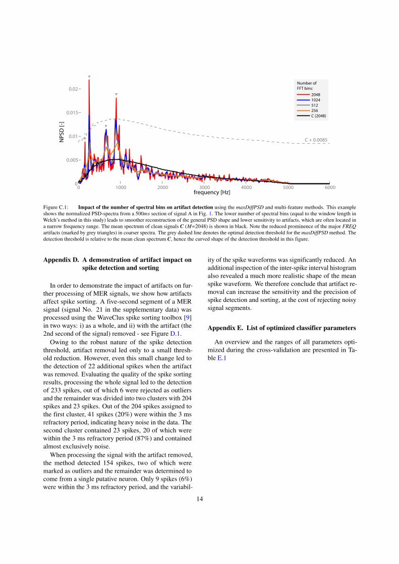
In order to estimate the PSD spectrum, we usedWelch’s method with the window length equal to thenumber of spectral bins in the discrete Fourier trans-form. The number of bins used throughout the paperwas M = 2048, which achieved good artifact detectionsensitivity, as shown in Fig. C.1. In this figure, wedemonstrate the impact of a decreasing number of spec-tral bins on the sensitivity of the resulting PSD spectrumto narrow-band MER signal components – which aretypical for the prevailing FREQ artifacts. Alternatively,other PSD estimation techniques (such as parametricestimation or other methods), or time-frequency analy-sis, may be utilized in future studies in order to achievehigher sensitivity to artifacts, while preserving good tem-poral resolution.

13

0 1000 2000 3000 4000 5000 60000

0.005

0.01

0.015

0.02

frequency [Hz]

NPS

D [-

]

2048

Number of FFT bins:

1024512256C (2048)

C + 0.0085

Figure C.1: Impact of the number of spectral bins on artifact detection using the maxDiffPSD and multi-feature methods. This exampleshows the normalized PSD-spectra from a 500ms section of signal A in Fig. 1. The lower number of spectral bins (equal to the window length inWelch’s method in this study) leads to smoother reconstruction of the general PSD shape and lower sensitivity to artifacts, which are often located ina narrow frequency range. The mean spectrum of clean signals C (M=2048) is shown in black. Note the reduced prominence of the major FREQartifacts (marked by grey triangles) in coarser spectra. The grey dashed line denotes the optimal detection threshold for the maxDiffPSD method. Thedetection threshold is relative to the mean clean spectrum C, hence the curved shape of the detection threshold in this figure.

Appendix D. A demonstration of artifact impact onspike detection and sorting

In order to demonstrate the impact of artifacts on fur-ther processing of MER signals, we show how artifactsaffect spike sorting. A five-second segment of a MERsignal (signal No. 21 in the supplementary data) wasprocessed using the WaveClus spike sorting toolbox [9]in two ways: i) as a whole, and ii) with the artifact (the2nd second of the signal) removed - see Figure D.1.

Owing to the robust nature of the spike detectionthreshold, artifact removal led only to a small thresh-old reduction. However, even this small change led tothe detection of 22 additional spikes when the artifactwas removed. Evaluating the quality of the spike sortingresults, processing the whole signal led to the detectionof 233 spikes, out of which 6 were rejected as outliersand the remainder was divided into two clusters with 204spikes and 23 spikes. Out of the 204 spikes assigned tothe first cluster, 41 spikes (20%) were within the 3 msrefractory period, indicating heavy noise in the data. Thesecond cluster contained 23 spikes, 20 of which werewithin the 3 ms refractory period (87%) and containedalmost exclusively noise.

When processing the signal with the artifact removed,the method detected 154 spikes, two of which weremarked as outliers and the remainder was determined tocome from a single putative neuron. Only 9 spikes (6%)were within the 3 ms refractory period, and the variabil-

ity of the spike waveforms was significantly reduced. Anadditional inspection of the inter-spike interval histogramalso revealed a much more realistic shape of the meanspike waveform. We therefore conclude that artifact re-moval can increase the sensitivity and the precision ofspike detection and sorting, at the cost of rejecting noisysignal segments.

Appendix E. List of optimized classifier parameters

An overview and the ranges of all parameters opti-mized during the cross-validation are presented in Ta-ble E.1

14

0 0.5 1 1.5 2 2.5 3 3.5 4 4.5 5−300

−200

−100

0

100

200

300

MER

[a.u

.]

time [s]

20 40 60

−200

−100

0

100

200

20 40 60time [samples]

20 40 60

−200

−100

0

100

200

00 0

time [samples]

A

B Cwhole signal artifact-free signal

spikes from whole signal

spikes from artifact-free signal

cluster 1 cluster 2 cluster 1

Figure D.1: Impact of artifacts on spike detection and sorting using the WaveClus toolbox [9]. A) A raw MER signal with a detectedone-second artifact marked in light grey. The blue/red marks (top) denote 227 spikes detected using the blue threshold on the whole signal and sortedautomatically into two clusters. Longer marks denote 97 spikes undetected in the artifact-free scenario. The orange marks (bottom) denote 152spikes, detected on the artifact-free signal using the orange dashed threshold. In this case, longer marks denote 22 spikes undetected on the wholesignal. B) Clustering result on the whole signal: all detected spike shapes in grey, overlaid by the cluster mean. Out of the 204 spikes assigned tothe first cluster, 41 spikes (20%) were within the 3ms refractory period, indicating heavy noise in the data. Clear amplitude clipping and technicalcharacter can be seen in cluster 2, which contains exclusively noise spikes. C) Spike sorting after artifact removal shows much more consistent spikeshapes, with lower variability around the mean spike waveform (orange).

15

0 2 4 6 8 10

2

1.5

1

0.5

0

−0.5

−1

−1.5

−2

−2.5

−3

−3.5

−4

−4.5

−5

−5.5

−6

−6.5

−7

−7.5

−8

−8.5

−9

−9.5

−10

dept

h [m

m]

0 2 4 6 8 10

central

0 2 4 6 8 10

lateral

0 2 4 6 8 10

medial

0 2 4 6 8 10

posterior

time [s]

Figure D.2: Example of a single DBS MER exploration annotated using the presented extension of the COV method (window length 0.25 s,threshold 1.2).

Table E.1: Overview of optimized classifier parameters and values

classifier optimized parameters

stationary method: i) COV (covariance, Aboy) or ii) SWT (wavelets, Guarnizo)segmentation segment length: .25,.33,.5,1

aggregation threshold: for .25 s window: 1, 2, 3, 4, for .33 s 1, 2, 3, for .5 s 1,2threshold for COV: <.8, 3.5>in .1 stepsthreshold for SWT: <9.5, 13>in .1 steps

diffPSD threshold: <0,0.025>in 0.0005 steps

decision tree split criterion: i) Gini’s diversity index ii) max. deviance reductionmin size of parent node: 1, 100, 200, ...,500, 100, 1500, 5000min. leaf size: 1, 250, 500, 750,...,2500 maximum up to half of current parent node min. size

SVM feature selection criterion: quadratic, linear, mahalanobisfeature selection stopping tolerance: .001, .005, .01SVM method: i) Sequential minimal optimization or ii) least squaresSVM kernel: i) linear ii) radial basis function (RBF)SVM kernel sigma (only for RBF): .5,1,2

Boosting algorithm: AdaBoostM1, LogitBoost, GentleBoost, RobustBoost, Bagnumber of learners: 10, 20,...,50,75,150,200,250learning rate: .1, .4, .7, 1RobustBoost error goal: .05, .1, .15, .2RobustBoost error max margin: .01, .05,.1

16

Algorithm 1 Identification of the maximum componentfrom the adjacency matrix

input: E; m*m adjacency matrix, m is number ofsegmentsoutput: max comp; indices of maximum component

comp =zeros(1,m); % denotes which segment belongs towhich componentact comp = 0; % Actual componentwhile any(comp == 0) do

% loop as long as there are unassigned segmentsopen = first zero in compclosed = [ ]act comp = act comp + 1while NOT isempty(open) do

% assign actual comp. to actual segmentcomp(open(1)) = act comp% expand current state (all segments adjacent tocurrent segment)children = find(E(open(1),:))% take the first element from open, find to whichsegments exists a direct pathfor ch in children do

if ch not in open OR closed thenopen = [open ch] % add ch to open

end ifend for

% move current node from open to closedclosed = [closed cur]open = open(2:end)

end whileend while

% find the largest componentcomp len = zeros(1,act comp)for cur in 1:act comp do

comp len(cur) = sum(comp == cur)end for[∼,max comp] = max(comp len)return max comp

17

References

[1] K. Slavin, J. Holsapple, Micro electrode Techniques EquipmentComponents and Systems, in: Z. Israel, K. Burchiel (Eds.), Mi-croelectrode Recording in Movement Disorder Surgery, Thieme,2004, pp. 14–27.

[2] W. C. Stacey, S. Kellis, B. Greger, C. R. Butson, P. R. Patel,T. Assaf, T. Mihaylova, S. Glynn, Potential for unreliable inter-pretation of EEG recorded with microelectrodes, Epilepsia 54 (8)(2013) 1391–1401. doi:10.1111/epi.12202.

[3] M. E. J. Obien, K. Deligkaris, T. Bullmann, D. J. Bakkum,U. Frey, Revealing neuronal function through microelectrodearray recordings, Frontiers in Neuroscience 8 (January) (2015)1–30. doi:10.3389/fnins.2014.00423.

[4] A. L. Benabid, P. Pollak, D. Gao, D. Hoffmann, P. Limousin,E. Gay, I. Payen, A. Benazzouz, Chronic electrical stimulation ofthe ventralis intermedius nucleus of the thalamus as a treatmentof movement disorders., J Neurosurg 84 (2) (1996) 203–214.doi:10.3171/jns.1996.84.2.0203.

[5] A. Abosch, L. Timmermann, S. Bartley, H. G. Rietkerk, D. Whit-ing, P. J. Connolly, D. Lanctin, M. I. Hariz, An internationalsurvey of deep brain stimulation procedural steps, Stereotac-tic and Functional Neurosurgery 91 (1) (2013) 1–11. doi:

10.1159/000343207.[6] J. Martinez, C. Pedreira, M. J. Ison, R. Quian Quiroga, Realistic

simulation of extracellular recordings, Journal of NeuroscienceMethods 184 (2009) 285–293. doi:10.1016/j.jneumeth.

2009.08.017.[7] L. a. Camunas-Mesa, R. Q. Quiroga, A detailed and fast model

of extracellular recordings., Neural computation 25 (2013) 1191–212. doi:10.1162/NECO\_a\_00433.

[8] K. D. Harris, D. A. Henze, J. Csicsvari, H. Hirase, G. Buzsaki,Accuracy of tetrode spike separation as determined by simulta-neous intracellular and extracellular measurements., Journal ofneurophysiology 84 (1) (2000) 401–14.

[9] R. Q. Quiroga, Z. Nadasdy, Y. Ben-Shaul, Unsupervised spikedetection and sorting with wavelets and superparamagneticclustering., Neural computation 16 (2004) 1661–1687. doi:

10.1162/089976604774201631.[10] U. Rutishauser, E. M. Schuman, A. N. Mamelak, Online detec-

tion and sorting of extracellularly recorded action potentials inhuman medial temporal lobe recordings, in vivo, Journal of Neu-roscience Methods 154 (1-2) (2006) 204–224. arXiv:0604033,doi:10.1016/j.jneumeth.2005.12.033.

[11] J. Wild, Z. Prekopcsak, T. Sieger, D. Novak, R. Jech, Perfor-mance comparison of extracellular spike sorting algorithms forsingle-channel recordings, Journal of Neuroscience Methods203 (2) (2012) 369–376. doi:10.1016/j.jneumeth.2011.

10.013.[12] K. Dolan, H. C. F. Martens, P. R. Schuurman, L. J. Bour, Au-

tomatic noise-level detection for extra-cellular micro-electroderecordings, Medical and Biological Engineering and Computing47 (7) (2009) 791–800. doi:10.1007/s11517-009-0494-4.

[13] M. Lourens, H. Meijer, M. Contarino, P. van den Munckhof,P. Schuurman, S. van Gils, L. Bour, Functional neuronal activityand connectivity within the subthalamic nucleus in Parkinson’sdisease, Clinical Neurophysiology 124 (5) (2013) 967–981. doi:10.1016/j.clinph.2012.10.018.

[14] A. Zaidel, A. Spivak, B. Grieb, H. Bergman, Z. Israel, Subthala-mic span of β oscillations predicts deep brain stimulation efficacyfor patients with Parkinson’s disease, Brain 133 (7) (2010) 2007–2021. doi:10.1093/brain/awq144.

[15] C. Seifried, L. Weise, R. Hartmann, Intraoperative microelec-trode recording for the delineation of subthalamic nucleus to-

pography in Parkinson’s disease, Brain stimulation 5 (3) (2012)378–387. doi:10.1016/j.brs.2011.06.002.

[16] K. J. Weegink, P. a. Bellette, J. J. Varghese, P. a. Silburn,P. a. Meehan, A. P. Bradley, Efficient Micro-electrode Record-ing Modeling using a Filtered Point Process, arXiv (2013) 1–22arXiv:1307.5250.

[17] A. Moran, I. Bar-Gad, H. Bergman, Z. Israel, Real-time refine-ment of subthalamic nucleus targeting using Bayesian decision-making on the root mean square measure., Mov Disord 21 (9)(2006) 1425–1431. doi:10.1002/mds.20995.

[18] A. Zaidel, A. Spivak, L. Shpigelman, H. Bergman, Z. Israel,Delimiting subterritories of the human subthalamic nucleusby means of microelectrode recordings and a Hidden MarkovModel., Mov Disord 24 (12) (2009) 1785–1793. doi:10.1002/mds.22674.

[19] A. Moran, H. Bergman, Z. Israel, I. Bar-Gad, Subthalamic nu-cleus functional organization revealed by parkinsonian neuronaloscillations and synchrony, Brain 131 (12) (2008) 3395–3409.doi:10.1093/brain/awn270.

[20] H. Cagnan, K. Dolan, X. He, M. F. Contarino, R. Schuurman,P. van den Munckhof, W. J. Wadman, L. Bour, H. C. F. Martens,Automatic subthalamic nucleus detection from microelectroderecordings based on noise level and neuronal activity., J Neu-ral Eng 8 (4) (2011) 46006. doi:10.1088/1741-2560/8/4/046006.

[21] R. Verhagen, D. G. Zwartjes, T. Heida, E. C. Wiegers, M. F.Contarino, R. M. de Bie, P. van den Munckhof, P. R. Schuurman,P. H. Veltink, L. J. Bour, Advanced target identification in STN-DBS with beta power of combined local field potentials andspiking activity, Journal of Neuroscience Methods 253 (2015)116–125. doi:10.1016/j.jneumeth.2015.06.006.

[22] J. H. Falkenberg, J. McNames, Segmentation of extracellular mi-croelectrode recordings with equal power, in: Proceedings of the25th Annual International Conference of the IEEE Engineeringin Medicine and Biology Society, Vol. 3, 2003, pp. 2475–2478.

[23] M. Aboy, J. H. Falkenberg, An automatic algorithm for stationarysegmentation of extracellular microelectrode recordings, Medicaland Biological Engineering and Computing 44 (6) (2006) 511–515. doi:10.1007/s11517-006-0052-2.

[24] C. Guarnizo, A. a. Orozco, G. Castcllanos, Microelectrode sig-nals segmentation using stationary wavelet transform, BioMed-ical Engineering and Informatics: New Development and theFuture - Proceedings of the 1st International Conference onBioMedical Engineering and Informatics, BMEI 2008 2 (2008)450–454. doi:10.1109/BMEI.2008.363.

[25] E. Bakstein, J. Schneider, T. Sieger, D. Novak, J. Wild, R. Jech,Supervised segmentation of microelectrode recording artifacts us-ing power spectral density, in: Proc. of 37th Annual InternationalConference of the IEEE Engineering in Medicine and BiologySociety, At Milano, Italy, Vol. 2015-Novem, IEEE, 2015, pp.1524–1527. doi:10.1109/EMBC.2015.7318661.

[26] K. J. Paralikar, C. R. Rao, R. S. Clement, New approaches toeliminating common-noise artifacts in recordings from intracorti-cal microelectrode arrays: Inter-electrode correlation and virtualreferencing, Journal of Neuroscience Methods 181 (1) (2009)27–35. doi:10.1016/j.jneumeth.2009.04.014.

[27] U. Egert, T. Knott, C. Schwarz, M. Nawrot, a. Brandt, S. Rot-ter, M. Diesmann, MEA-Tools: An open source toolbox forthe analysis of multi-electrode data with MATLAB, Journal ofNeuroscience Methods 117 (1) (2002) 33–42. doi:10.1016/S0165-0270(02)00045-6.

[28] D. a. Wagenaar, S. M. Potter, Real-time multi-channel stimu-lus artifact suppression by local curve fitting, Journal of Neu-roscience Methods 120 (2) (2002) 113–120. doi:10.1016/

S0165-0270(02)00149-8.

18

[29] D. Wagenaar, T. DeMarse, S. Potter, MeaBench: A toolset formulti-electrode data acquisition and on-line analysis, in: Confer-ence Proceedings. 2nd International IEEE EMBS Conference onNeural Engineering, 2005., Vol. 2005, IEEE, 2005, pp. 518–521.doi:10.1109/CNE.2005.1419673.

[30] I. Gligorijevic, M. Welkenhuysen, D. Prodanov, S. Musa, B. Nut-tin, W. Eberle, C. Bartic, S. V. Huffel, Neural signal analysis andartifact removal in single and multichannel in-vivo deep brainrecordings, Neurosurgery (2009) 8–11.

19