methods and models for combinatorial optimization...

Methods and Models for Combinatorial OptimizationModeling by Linear Programming

Luigi De Giovanni, Marco Di Summa

Dipartimento di Matematica, Universita di Padova

De Giovanni, Di Summa MeMoCO 1 / 35

Mathematical Programming Models

A mathematical programming model describes the characteristics ofthe optimal solution of an optimization problem by means ofmathematical relations. It provides a formulation and a basis forstandard optimization algorithms.

Sets: they group the elements of the system

Parameters: the data of the problem, which represent the knownquantities depending on the elements of the system.

Decision (or control) variables: the unknown quantities, on whichwe can act in order to find different possible solutions to the problem.

Constraints: mathematical relations that describe solution fasibilityconditions (they distinguish acceptable combinations of values of thevariables).

Objective function: quantity to maximize or minimize, as a functionof the decision variables.


Linear Programming models

Mathematical programming models where:

objective function is a linear expression of the decision variables;

constraints are a system of linear equations and/or inequalities.

Classification of linear programming models:

Linear Programming models (LP): all the variables can take real(R) values;

Integer Linear Programming models (ILP): all the variables cantake integer (Z) values only;

Mixed Integer Linear Programming models (MILP): somevariables can take real values and others can take integer values only.

Linearity limits expressiveness but allows faster solution techniques!


An LP model for a simple CO problem

Example

A perfume firm produces two new items by mixing three essences: rose,lily and violet. For each decaliter of perfume one, it is necessary to use 1.5liters of rose, 1 liter of lily and 0.3 liters of violet. For each decaliter ofperfume two, it is necessary to use 1 liter of rose, 1 liter of lily and 0.5liters of violet. 27, 21 and 9 liters of rose, lily and violet (respectively) areavailable in stock. The company makes a profit of 130 euros for eachdecaliter of perfume one sold, and a profit of 100 euros for each decaliterof perfume two sold. The problem is to determine the optimal amount ofthe two perfumes that should be produced.

max 130 xone + 100 xtwo objective functions.t. 1.5 xone + xtwo ≤ 27 availability of rose

xone + xtwo ≤ 21 availability of lily0.3 xone + 0.5 xtwo ≤ 9 availability of violet

xone , xtwo ≥ 0 domains of the variables


One possible modeling schema: optimal production mix

set I : resource set I = {rose, lily , violet}set J: product set J = {one, two}

parameters Di : availability of resource i ∈ I e.g. Drose = 27

parameters Pj : unit profit for product j ∈ J e.g. Pone = 130

parameters Qij : amount of resource i ∈ I required for each unit ofproduct j ∈ J e.g. Qrose one = 1.5, Qlily two = 1

variables xj : amount of product j ∈ J xone , xtwo

max∑j∈J

Pjxj

s.t.∑j∈J

Qijxj ≤ Di ∀ i ∈ I

xj ∈ R+ [ Z+ | {0, 1} ] ∀ j ∈ J


The diet problem

Example

We need to prepare a diet that supplies at least 20 mg of proteins. 30 mgof iron and 10 mg of calcium. We have the opportunity of buyingvegetables (containing 5 mg/kg of proteins, 6 mg/Kg of iron e 5 mg/Kgof calcium, cost 4 E/Kg), meat (15 mg/kg of proteins, 10 mg/Kg of iron e3 mg/Kg of calcium, cost 10 E/Kg) and fruits (4 mg/kg of proteins, 5mg/Kg of iron e 12 mg/Kg of calcium, cost 7 E/Kg). We want todetermine the minimum cost diet.

min 4 xV + 10 xM + 7 xF costs.t. 5 xV + 15 xM + 4 xF ≥ 20 proteins

6 xV + 10 xM + 5 xF ≥ 30 iron5 xV + 3 xM + 12 xF ≥ 10 calciumxV , xM , xF ≥ 0 domains of the variables


One possible modeling schema: minimum cost covering

set I : available resources I = {V ,M,F}set J: request set J = {proteins, iron, calcium}

parameters Ci : unit cost of resource i ∈ I

parameters Rj : requested amount of j ∈ J

parameters Aij : amount of request j ∈ J satisfied by one unit ofresource i ∈ I

variables xi : amount of resource i ∈ I

min∑i∈I

Cixi

s.t. ∑i∈I

Aijxi ≥ Dj ∀ j ∈ J

xi ∈ R+ [ Z+ | {0, 1} ] ∀ i ∈ I


The transportation problem

Example

A company produces refrigerators in three different factories (A, B and C)and need to move them to four stores (1, 2, 3, 4). The production offactories A, B and C is 50, 70 and 20 units, respectively. Stores 1, 2, 3 and4 require 10, 60, 30 e 40 units, respectively. The costs in Euros to moveone refrigerator from a factory to stores 1, 2, 3 and 4 are the following:

from A: 6, 8, 3, 4from B: 2, 3, 1, 3from C: 2, 4, 6, 5

The company asks us to formulate a minimum cost transportation plan.


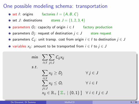
One possible modeling schema: transportation

set I : origins factories I = {A,B,C}set J: destinations stores J = {1, 2, 3, 4}

parameters Oi : capacity of origin i ∈ I factory production

parameters Dj : request of destination j ∈ J store request

parameters Cij : unit transp. cost from origin i ∈ I to destination j ∈ J

variables xij : amount to be transported from i ∈ I to j ∈ J

min∑i∈I

∑j∈J

Cijxij

s.t. ∑i∈I

xij ≥ Dj ∀ j ∈ J∑j∈J

xij ≤ Oi ∀ i ∈ I

xij ∈ R+ [ Z+ | {0, 1} ] ∀ i ∈ I j ∈ J


Fixed costs

Example

A supermarket chain has a budget W available for opening new stores.Preliminary analyses identified a set I of possible locations. Opening astore in i ∈ I has a fixed cost Fi (land acquisition, other administrativecosts etc.) and a variable cost Ci per 100 m2 of store. Once opened, thestore in i guarantees a revenue of Ri per 100 m2. Determine the subset oflocation where a store has to be opened and the related size in order tomaximize the total revenue, taking into account that at most K stores canbe opened.


Modeling fixed costs: binary/boolean variablesset I : potential locations

parameters W , Fi , Ci , Ri , “large-enough” M

variables xi : size (in 100 m2) of the store in i ∈ I

variables yi : taking value 1 if a store is opened in i ∈ I (xi > 0), 0 otherwise

max∑i∈I

Ri xi

s.t. ∑i∈I

Ci xi + Fi yi ≤W budget

xi ≤ M yi ∀ i ∈ I BigM constraint / relate xi to yi∑i∈I

yi ≤ K max number of stores

xi ∈ R+, yi ∈ {0, 1} ∀ i ∈ I


Moving scaffolds between construction yards

A construction company has to move the scaffolds from three closing building sites (A,B, C) to three new building sites (1, 2, 3). The scaffolds consist of iron rods: in thesites A, B, C there are respectively 7000, 6000 and 4000 iron rods, while the new sites 1,2, 3 need 8000, 5000 and 4000 rods respectively. The following table provide the cost ofmoving one iron rod from a closing site to a new site:

Costs (euro cents) 1 2 3A 9 6 5B 7 4 9C 4 6 3

Trucks can be used to move the iron rods from one site to another site. Each truck cancarry up to 10000 rods. Find a linear programming model that determine the minimumcost transportation plan, taking into account that:

using a truck causes an additional cost of 50 euros;

only 4 trucks are available (and each of them can be used only for a single pair ofclosing site and new site);

the rods arriving in site 2 cannot come from both sites A and B;

it is possible to rent a fifth truck for 65 euros (i.e., 15 euros more than the othertrucks).


Moving scaffolds between construction yards: elementsSets:

I : closing sites (origins);

J: news sites (destinations ).

Parameters:

Cij : unit cost (per rod) for transportation from i ∈ I to j ∈ J;

Di : number of rods available at origin i ∈ I ;

Rj : number of rods required at destination j ∈ J;

F : fixed cost for each truck;

N: number of trucks;

L: fixed cost for the rent of an additional truck;

K : truck capacity.

Decision variables:

xij : number of rods moved from i ∈ I to j ∈ J;

yij : binary, values 1 if a truck from i ∈ I to j ∈ J is used, 0 otherwise.

z : binary, values 1 if the additional truck is used, 0 otherwise.De Giovanni, Di Summa MeMoCO 13 / 35

Moving scaffolds between construction yards: MILP model

[Suggestion: compose transportation and fixed cost schemas]

min∑

i∈I ,j∈JCij xij + F

∑i∈I ,j∈J

yij + (L− F ) z

s.t.∑i∈I

xij ≥ Rj ∀ j ∈ J∑j∈J

xij ≤ Di ∀ i ∈ I

xij ≤ K yij ∀ i ∈ I , j ∈ J∑i∈I ,j∈J

yij ≤ N + z

xij ∈ Z+ ∀ i ∈ I , j ∈ Jyij ∈ {0, 1} ∀ i ∈ I , j ∈ Jz ∈ {0, 1}


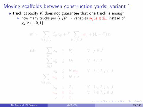
Moving scaffolds between construction yards: variant 1truck capacity K does not guarantee that one truck is enough

I how many trucks per (i , j)? ⇒ variables wij , z ∈ Z+ instead ofyij , z ∈ {0, 1}

min∑

i∈I ,j∈JCij xij + F

∑i∈I ,j∈J

wij + (L− F ) z

s.t.∑i∈I


xij ≤ Di ∀ i ∈ I

xij ≤ K wij ∀ i ∈ I , j ∈ J∑i∈I ,j∈J

wij ≤ N + z

xij ∈ Z+ ∀ i ∈ I , j ∈ Jwij ∈ Z+ ∀ i ∈ I , j ∈ Jz ∈ Z+


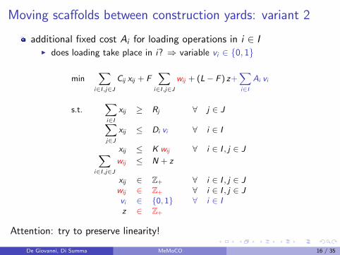
Moving scaffolds between construction yards: variant 2

additional fixed cost Ai for loading operations in i ∈ II does loading take place in i? ⇒ variable vi ∈ {0, 1}

min∑

i∈I ,j∈J

Cij xij + F∑

i∈I ,j∈J

wij + (L− F ) z+∑i∈I

Ai vi

s.t.∑i∈I


xij ≤ Di vi ∀ i ∈ I

xij ≤ K wij ∀ i ∈ I , j ∈ J∑i∈I ,j∈J

wij ≤ N + z

xij ∈ Z+ ∀ i ∈ I , j ∈ Jwij ∈ Z+ ∀ i ∈ I , j ∈ Jvi ∈ {0, 1} ∀ i ∈ Iz ∈ Z+

Attention: try to preserve linearity!


Emergency location

A network of hospitals has to cover an area with the emergency service. The areahas been divided into 6 zones and, for each zone, a possible location for theservice has been identified. The average distance, in minutes, from every zone toeach potential service location is shown in the following table.

Loc. 1 Loc. 2 Loc. 3 Loc. 4 Loc. 5 Loc. 6Zone 1 5 10 20 30 30 20Zone 2 10 5 25 35 20 10Zone 3 20 25 5 15 30 20Zone 4 30 35 15 5 15 25Zone 5 30 20 30 15 5 14Zone 6 20 10 20 25 14 5

It is required each zone has an average distance from a emergency service of at

most 15 minutes. The hospitals ask us for a service opening scheme that

minimizes the number of emergency services in the area.


Emergency location: MILP model from covering schema

I set od potential locations (I = {1, 2, ..., 6}).

xi variables, values 1 if service is opened at location i ∈ I , 0 otherwise.

min x1 + x2 + x3 + x4 + x5 + x6

s.t.x1 + x2 ≥ 1 (cover zone 1)x1 + x2 + x6 ≥ 1 (cover zone 2)

x3 + x4 ≥ 1 (cover zone 3)x3 + x4 + x5 ≥ 1 (cover zone 4)

x4 + x5 + x6 ≥ 1 (cover zone 5)x2 + x5 + x6 ≥ 1 (cover zone 6)

x1 , x2 , x3 , x4 , x5 , x6 ∈ {0, 1} (domain)


TLC antennas location

A telephone company wants to install antennas in some sites in order to cover six areas.Five possible sites for the antennas have been detected. After some simulations, theintensity of the signal coming from an antenna placed in each site has been establishedfor each area. The following table summarized these intensity levels:

area 1 area 2 area 3 area 4 area 5 area 6site A 10 20 16 25 0 10site B 0 12 18 23 11 6site C 21 8 5 6 23 19site D 16 15 15 8 14 18site E 21 13 13 17 18 22

Receivers recognize only signals whose level is at least 18. Furthermore, it is not possible

to have more than one signal reaching level 18 in the same area, otherwise this would

cause an interference. Finally, an antenna can be placed in site E only if an antenna is

installed also in site D (this antenna would act as a bridge). The company wants to

determine where antennas should be placed in order to cover the maximum number of

areas.


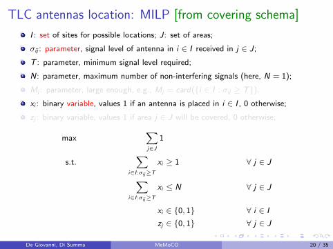
TLC antennas location: MILP [from covering schema]

I : set of sites for possible locations; J: set of areas;

σij : parameter, signal level of antenna in i ∈ I received in j ∈ J;

T : parameter, minimum signal level required;

N: parameter, maximum number of non-interfering signals (here, N = 1);

Mj : parameter, large enough, e.g., Mj = card({i ∈ I : σij ≥ T}).

xi : binary variable, values 1 if an antenna is placed in i ∈ I , 0 otherwise;

zj : binary variable, values 1 if area j ∈ J will be covered, 0 otherwise;

max∑j∈J

1

s.t.∑

i∈I :σij≥T

xi ≥ 1 ∀ j ∈ J

∑i∈I :σij≥T

xi ≤ N ∀ j ∈ J

xi ∈ {0, 1} ∀ i ∈ I

zj ∈ {0, 1} ∀ j ∈ J


TLC antennas location: MILP [from covering schema]

I : set of sites for possible locations; J: set of areas;

σij : parameter, signal level of antenna in i ∈ I received in j ∈ J;

T : parameter, minimum signal level required;

N: parameter, maximum number of non-interfering signals (here, N = 1);

Mj : parameter, large enough, e.g., Mj = card({i ∈ I : σij ≥ T}).

xi : binary variable, values 1 if an antenna is placed in i ∈ I , 0 otherwise;

zj : binary variable, values 1 if area j ∈ J will be covered, 0 otherwise;

max∑j∈J

zj

s.t.∑

i∈I :σij≥T

xi ≥ zj ∀ j ∈ J

∑i∈I :σij≥T

xi ≤ N+Mj(1− zj) ∀ j ∈ J

xi ∈ {0, 1} ∀ i ∈ I

zj ∈ {0, 1} ∀ j ∈ J


Four Italian friends [from La Settimana Enigmistica]Andrea, Bruno, Carlo and Dario share an apartment and read four newspapers: “La

Repubblica”, “Il Messaggero”, “La Stampa” and “La Gazzetta dello Sport” before going

out. Each of them wants to read all newspapers in a specific order. Andrea starts with

“La Repubblica” for one hour, then he reads “La Stampa” for 30 minutes, “Il

Messaggero” for two minutes and then “La Gazzetta dello Sport” for 5 minutes. Bruno

prefers to start with “La Stampa” for 75 minutes; he then has a look at “Il Messaggero”

for three minutes, then he reads “La Repubblica” for 25 minutes and finally “La

Gazzetta dello Sport” for 10 minutes. Carlo starts with “Il Messaggero” for 5 minutes,

then he reads “La Stampa” for 15 minutes, “La Repubblica” for 10 minutes and “La

Gazzetta dello Sport” for 30 minutes. Finally, Dario starts with “La Gazzetta dello

Sport” for 90 minutes and then he dedicates just one minute to each of “La

Repubblica”, “La Stampa” and “Il Messaggero” in this order. The preferred order is so

important that each is willing to wait and read nothing until the newspaper that he

wants becomes available. Moreover, none of them would stop reading a newspaper and

resume later. By taking into account that Andrea gets up at 8:30, Bruno and Carlo at

8:45 and Dario at 9:30, and that they can wash, get dressed and have breakfast while

reading the newspapers, what is the earliest time they can leave home together?


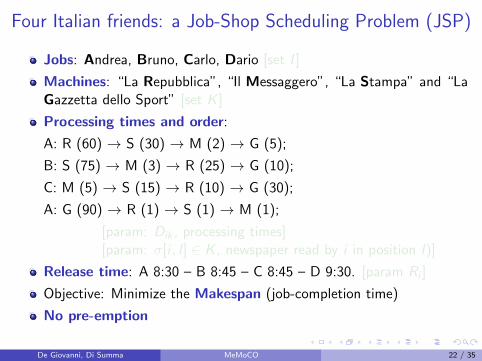
Four Italian friends: a Job-Shop Scheduling Problem (JSP)

Jobs: Andrea, Bruno, Carlo, Dario [set I ]

Machines: “La Repubblica”, “Il Messaggero”, “La Stampa” and “LaGazzetta dello Sport” [set K ]

Processing times and order:

A: R (60) → S (30) → M (2) → G (5);

B: S (75) → M (3) → R (25) → G (10);

C: M (5) → S (15) → R (10) → G (30);

A: G (90) → R (1) → S (1) → M (1);

[param: Dik , processing times][param: σ[i , l ] ∈ K , newspaper read by i in position l)]

Release time: A 8:30 – B 8:45 – C 8:45 – D 9:30. [param Ri ]

Objective: Minimize the Makespan (job-completion time)

No pre-emption


LP model for JSP

hik : start time (in minutes after 8:30) of i ∈ I on k ∈ K ;

y : completion time (in minutes after 8:30);

xijk : binary, 1 if i ∈ I precedes j ∈ I on k ∈ K , 0 otherwise.

min y

s.t. y ≥ hi σ[i ,|K |] + Di σ[i ,|K |] ∀ i ∈ I

hi σ[i ,l ] ≥ hi σ[i ,l−1] + Di σ[i ,l−1] ∀ i ∈ I , l = 2...|K |hi σ[i ,1] ≥ Ri ∀ i ∈ I

hik ≥ hjk + Djk −M xijk ∀ k ∈ K , i ∈ I , j ∈ I : i 6= j

hjk ≥ hik + Dik −M (1− xijk) ∀ k ∈ K , i ∈ I , j ∈ I : i 6= j

y ∈ R+

hik ∈ R+ ∀ k ∈ K , i ∈ I

xijk ∈ {0, 1} ∀ k ∈ K , i ∈ I , j ∈ I : i 6= j


Project scheduling in the boatyard industryConstructing a boat requires the completion of the following operations :

Operations Duration PrecedencesA 2 noneB 4 AC 2 AD 5 AE 3 B,CF 3 EG 2 EH 7 D,E,GI 4 F,G

Some of the operations are alternative to each other. In particular, only one of B and C

needs to be executed, and only one of F and G needs to be executed. Furthermore, if

both C and G are executed, the duration of I increases by 2 days. The table also shows

the precedences for each operation (i.e., operations that must be completed before the

beginning of the new operation). For instance, H can start only after the completion of

E, D and G (if G will be executed). Write a linear programming model that can be used

to decide which operations should be executed in order to minimize the total duration of

the construction of the boat.


Project scheduling in the boatyard industry: hints

min z

s.t. z ≥ ti ∀i ∈ A...I

tA ≥ dA

tB ≥ tA + dB −M(1− yB)

tC ≥ tA + dC −M(1− yC )

tD ≥ tA + dD

tE ≥ tB + dE

tE ≥ tC + dE

tF ≥ tE + dF −M(1− yF )

tG ≥ tA + dG −M(1− yG )

tH ≥ tD + dH

tH ≥ tE + dH

tH ≥ tG + dH

tI ≥ tF + dI + 2yCG

tI ≥ tG + dI + 2yCG

yB + yC = 1

yF + yG = 1

yC + yG <= 1 + yCG

z, ti ≥ 0 ∀i ∈ {A...I}y . ∈ {0, 1}

where

ti completion time of operation i ∈ {A,B,C ,D,E ,F ,G ,H, I};yi 1 if operation i ∈ {B,C ,F ,G} is executed, 0 otherwise;

yCG 1 if both C and G are executed, 0 otherwise;

z completion time of the last operation;

di parameter indicating the duration of operation i ;

M sufficiently large constant.

Exercise: write a more general model for generic sets of operations and precedence.


A (shift) covering problem

The pharmacy federation wants to organize the opening shifts on publicholidays all over the region. The number of shifts is already decided, andthe number of pharmacies open on the same day has to be as balanced aspossible. Furthermore, every pharmacy is part of one shift only. Forinstance, if there are 12 pharmacies and the number of shifts is 3, everyshift will consist of 4 pharmacies. Pharmacies and users are thought asconcentrated in centroids (for instance, villages). For every centroid, thenumber of users and pharmacies are known. The distance between everyordered pair of centroids is also known. For the sake of simplicity, weignore congestion problems and we assume that every user will go to theclosest open pharmacy. The target is to determine the sifts so that thetotal distance covered by the users is minimized.


A (shift) covering problem: model 1yik : 1 if pharmacy j ∈ P takes part in shift k = 1 . . .K , 0 otherwise;

zijk : 1 if centroid i ∈ C uses pharmacy j ∈ P during shift k = 1 . . .K , 0 otherwise(notice: by optimality, z selects the nearest open pharmacy)

minK∑

k=1

∑i∈C

∑j∈P

Dijzijk (parameter Dij : distance from i to j)

s.t.K∑

k=1

yjk = 1 ∀ j ∈ P∑j∈P

zijk = 1 ∀ i ∈ C , k = 1 . . .K

xijk ≤ yjk ∀ i ∈ C , j ∈ P, k = 1 . . .K(b|P|/Kc ≤

∑j∈P

yjk ≤ d|P|/Ke ∀ k = 1 . . .K)

zijk , yjk ∈ {0, 1} ∀ i ∈ C , j ∈ P, k = 1 . . .K

Notice: the model has a polynomial number of variables and constraints but suffers from

symmetries, that is, the same “real” solution can be represented in many different ways, by

giving different names (i.e. value of k) to the same shifts.


A (shift) covering problem: model 2

P: set of all possible subsets of P (with balanced cardinality for balancing constraint)D(J): total distance covered by all users in C to reach the nearest pharmacy in J ∈ P

xJ : 1 if the set J ∈ P is selected as a shift, 0 otherwise;

min∑J∈P

DJxJ

s.t.∑J∈P

xJ = K

∑J∈P:j∈J

xJ = 1 ∀ j ∈ P

xJ ∈ {0, 1} ∀J ∈ P

Notice: the model does not suffer from symmetries (a shift is directly determined by the

defining subset), but has an exponential number of variables [we will see how to face this issue].


An energy flow problem

A company distributing electric energy has several power plants and distributingstations connected by wires. Each station i can:

produce pi kW of energy (pi = 0 if the station cannot produce energy);

distribute energy on a sub-network whose users have a total demand of dikW (di = 0 if the station serves no users);

carry energy from/to different stations.

The wires connecting station i to station j have a maximum capacity of uij kW

and a cost of cij euros for each kW carried by the wires. The company wants to

determine the minimum cost distribution plan, under the assumption that the

total amount of energy produced equals the total amount of energy required by

all sub-networks.


Network flows models: single commodity

Parameters: uij , cij and

G = (N,A), N = power/distribution stations, A = connections between stations

bv = dv − pv , v ∈ N [demand (bv > 0)/supply (< 0)/transshipment (= 0) node]

Variables:

xij amount of energy to flow on arc (i , j) ∈ A

min∑

(i,j)∈A

cijxij

s.t.∑

(i,v)∈A

xiv −∑

(v,j)∈A

xvj = bv ∀ v ∈ N

xij ≤ uij ∀ (i , j) ∈ A

xij ∈ R+

Minimum Cost Network Flow Problem


An multi-type energy flow problem

A company distributing electric energy has several power and distributing stationsconnected by wires. Each station produces/distributes different kinds of energy.Each station i can:

produce pki kW of energy of type k (it may be pki = 0);

distribute energy of type k on a sub-network whose users have a totaldemand of dk

i kW (it may be dki = 0);

carry energy from/to different stations.

Note that every station can produce and/or distribute different types of energy.

The wires connecting station i to station j have a maximum capacity of uij kW,

independently of the type of energy carried. The transportation cost depends both

on the pair of stations (i , j) and the type of energy k , and is equal to ckij euros for

each kW. The company wants to determine the minimum cost distribution plan,

under the assumption that, for each type of energy, the total amount produced

equals the total amount of energy of the same type required by all sub-networks.


Network flows models: multi-commodity

Parameters: uij , ckij , K (set of energy types or commodities) and

G = (N,A), N = power/distribution stations, A = connections between stations

bkv = dk

v − pkv , v ∈ N [demand (bk

v > 0)/supply (< 0)/transshipment (= 0) node]

Variables:

xkij amount of energy of type k to flow on arc (i , j) ∈ A

min∑k∈K

∑(i,j)∈A

ckij xkij

s.t.∑

(i,v)∈A

xkiv −

∑(v,j)∈A

xkvj = bk

v ∀ v ∈ N, ∀ k ∈ K

∑k∈K

xkij ≤ uij ∀ (i , j) ∈ A

xkij ∈ R+ ∀ (i , j) ∈ A, ∀ k ∈ K

Minimum Cost Network Multi-commodity Flow Problem


methods and models for combinatorial optimization...

Documents