methods and applications of pyrolysis modelling for ... science 44 methods and applications of...

•VIS

ION

S•SCIENCE•TEC

HN

OL

OG

Y•RESEARCHHIGHLI

GH

TS

Dissertation

44

Methods and applications of pyrolysis modelling for polymeric materialsAnna Matala

VTT SCIENCE 44

Methods and applications of pyrolysis modelling for polymeric materials

Anna Matala

Thesis for the degree of Doctor of Science (Technology) to be presented with due permission for public examination and criticism in Otakaari 1, at Aalto University School of Science, on the 15.11.2013 at 12 noon.

ISBN 978-951-38-8101-6 (Soft back ed.)

ISBN 978-951-38-8102-3 (URL: http://www.vtt.fi/publications/index.jsp)

VTT Science 44

ISSN-L 2242-119X

ISSN 2242-119X (Print)

ISSN 2242-1203 (Online)

Copyright © VTT 2013

JULKAISIJA – UTGIVARE – PUBLISHER

VTT

PL 1000 (Tekniikantie 4 A, Espoo)

02044 VTT

Puh. 020 722 111, faksi 020 722 7001

VTT

PB 1000 (Teknikvägen 4 A, Esbo)

FI-02044 VTT

Tfn. +358 20 722 111, telefax +358 20 722 7001

VTT Technical Research Centre of Finland

P.O. Box 1000 (Tekniikantie 4 A, Espoo)

FI-02044 VTT, Finland

Tel. +358 20 722 111, fax +358 20 722 7001

Kopijyvä Oy, Kuopio 2013

3

Methods and applications of pyrolysis modelling for polymeric materials

Pyrolyysimallinnuksen metodeita ja sovelluksia polymeereille. Anna Matala. Espoo 2013. VTT Science 44. 85 p. + app. 87 p.

Abstract

Fire is a real threat for people and property. However, if the risks can be identified

before the accident, the consequences can be remarkably limited. The

requirement of fire safety is particularly important in places with large number of

people and limited evacuation possibilities (e.g., ships and airplanes) and for

places where the consequences of fire may spread wide outside of the fire

location (e.g., nuclear power plants).

The prerequisite for reliable fire safety assessment is to be able to predict the

fire spread instead of prescribing it. For predicting the fire spread accurately, the

pyrolysis reaction of the solid phase must be modelled. The pyrolysis is often

modelled using the Arrhenius equation with three unknown parameters per each

reaction. These parameters are not material, but model specific, and therefore

they need to be estimated from the experimental small-scale data for each sample

and model individually.

The typical fuel materials in applications of fire safety engineers are not always

well-defined or characterised. For instance, in electrical cables, the polymer blend

may include large quantities of additives that change the fire performance of the

polymer completely. Knowing the exact chemical compound is not necessary for

an accurate model, but the thermal degradation and the release of combustible

gases should be identified correctly.

The literature study of this dissertation summarises the most important

background information about pyrolysis modelling and the thermal degradation of

the polymers needed for understanding the methods and results of this

dissertation. The articles cover developing methods for pyrolysis modelling and

testing them for various materials. The sensitivity of the model for the modelling

choices is also addressed by testing several typical modeller choices. The heat

release of unknown polymer blend is studied using Microscale Combustion

Calorimetry (MCC), and two methods are developed for effectively using the MCC

results in building an accurate reaction path. The process of pyrolysis modelling is

presented and discussed. Lastly, the methods of cable modelling are applied to a

large scale simulation of a cable tunnel of a Finnish nuclear power plant.

The results show that the developed methods are practical, produce accurate

fits for the experimental results, and can be used with different materials. Using

these methods, the modeller is able to build an accurate reaction path even if the

material is partly uncharacterised. The methods have already been applied to

simulating real scale fire scenarios, and the validation work is continuing.

Keywords pyrolysis modelling, simulation, polymer, cables, composites, probabilistic

risk assessment (PRA)

4

Pyrolyysimallinnuksen metodeita ja sovelluksia polymeereille

Methods and applications of pyrolysis modelling for polymeric materials. Anna Matala. Espoo 2013. VTT Science 44. 85 s. + liitt. 87 s.

Tiivistelmä

Tulipalot aiheuttavat todellisen uhan ihmisille ja omaisuudelle. Mikäli riskit voidaan

tunnistaa jo ennen onnettomuutta, tulipalon ikäviä seurauksia voidaan rajoittaa.

Paloturvallisuuden merkitys korostuu erityisesti paikoissa, joissa on paljon ihmisiä

ja rajoitetut evakuointimahdollisuudet (esim. laivat ja lentokoneet), ja laitoksissa,

joissa tulipalon seuraukset voivat levitä laajalle palopaikan ulkopuolellekin (esim.

ydinvoimalaitokset).

Jotta materiaalien palokäyttäytymistä voitaisiin luotettavasti tarkastella

erilaisissa olosuhteissa, pitää palon leviäminen pystyä ennustamaan sen sijaan,

että paloteho määrättäisiin ennalta. Palon leviämisen ennustamiseksi täytyy

materiaalin kiinteän faasin pyrolyysireaktiot tuntea ja mallintaa. Pyrolyysi

mallinnetaan usein käyttäen Arrheniuksen yhtälöä, jossa on kolme tuntematonta

parametria jokaista reaktiota kohti. Nämä parametrit eivät ole materiaali- vaan

mallikohtaisia, ja siksi ne täytyy estimoida kokeellisista pienen mittakaavan

kokeista jokaiselle näytteelle ja mallille erikseen.

Paloturvallisuusinsinöörin kannalta erityisen hankalaa on, että palavat

materiaalit eivät useinkaan ole hyvin määriteltyjä tai tunnettuja. Esimerkiksi

sähkökaapeleiden polymeeriseokset voivat sisältää suuria määriä erilaisia

lisäaineita, jotka vaikuttavat materiaalin palokäyttäytymiseen merkittävästi.

Kemiallisen koostumuksen tunteminen ei ole välttämätöntä luotettavan mallin

aikaansaamiseksi, mutta aineen lämpöhajoaminen ja erityisesti palavien kaasujen

vapautuminen tulisi tuntea tarkasti.

Väitöskirjan tiivistelmäosa kokoaa yhteen tärkeimmät taustatiedot

pyrolyysimallinnuksen ja polymeerien palokäyttäytymisen ymmärtämisen tueksi.

Tässä väitöstyössä on kehitetty menetelmiä pyrolyysiparametrien estimoimiseksi

ja näitä metodeita on testattu erilaisilla materiaaleilla. Mallinnusvalintojen

merkitystä mallin tarkkuuteen on myös tutkittu herkkyysanalyysin keinoin. Osittain

tuntemattomien polymeeriseosten lämmön vapautumista on tutkittu käyttäen

mikrokalorimetria. Mikrokalorimetritulosten hyödyntämiseksi kehitettiin kaksi

metodia, joiden avulla voidaan saada aikaan entistä tarkempia reaktiopolkuja.

Lopuksi pyrolyysimallinnusta on hyödynnetty sovellusesimerkissä suomalaisen

ydinvoimalan kaapelitilan täyden mittakaavan kaapelisimuloinneissa.

Tulokset osoittavat, että tässä työssä kehitetyt menetelmät ovat käytännöllisiä,

tuottavat riittävän tarkkoja sovituksia koetuloksille ja niitä voidaan soveltaa monien

erilaisten materiaalien mallintamiseen. Näitä menetelmiä käyttämällä mallintaja

pystyy mallintamaan tuntemattomienkin materiaalien palokäyttäytymistä riittävän

tarkasti. Menetelmiä on jo sovellettu todellisten, suuren mittakaavan

palotilanteiden simuloimiseksi, ja validointityö jatkuu edelleen.

Avainsanat pyrolyysimallinnus, simulaatiot, polymeerit, kaapelit, komposiitit,

todennäköisyyspohjainen riskianalyysi (PRA)

5

Preface

In spring 2007 I returned home from a job interview full of excitement; I had been

offered a summer job at the fire research team of VTT. I did not know much about

the work itself, but what could be "hotter" than a summer job playing with fire and

even getting paid for it! That summer I implemented the first version of my genetic

algorithm application for Matlab that has been extensively used throughout this

dissertation work. After the summer job, I progressed to be a Master‟s thesis

worker in the same team, and after graduation the work continued naturally

towards the PhD dissertation (I don‟t think anyone even asked me if I was

interested in doing a PhD, it just happened). During these years, I have had the

opportunity to get familiar with the fascinating topic of fire and pyrolysis modelling,

and had an opportunity to get to know many inspiring people. The learning has not

been fully successful – I still burn my fingers regularly, both at work and at home,

but I still love watching fire and burning things; who wouldn‟t?

There are so many great people I want to thank for contributing to my

dissertation. First of all, I would like to acknowledge my Professor Harri Ehtamo

from Aalto University School of Science, for supervising this PhD work, and the

pre-examiners, Dr. Richard E. Lyon and Dr. Brian Lattimer, for their valuable

comments. I would like to thank my thesis advisor and boss, Dr. Simo Hostikka

from VTT, who has been supervising my work at VTT ever since the summer of

2007. He has provided continuous support, patiently provided answers to my

never-ending questions and motivated me when my own ideas wained. At VTT,

I‟m also grateful to our technology manager Dr. Eila Lehmus, for making this

doctoral work possible and for her encouragement, Dr. Esko Mikkola for his

valuable comments on my dissertation manuscript and for being the best office

mate, and Dr. Johan Mangs and Dr. Tuula Hakkarainen for guidance and

company during the long hours of experimental work. My team (past and current)

deserves a special acknowledgement for the great work ambience, and for making

it easy and pleasant place to work; thank you Simo, Tuula, Esko, Johan, Topi,

Antti, Terhi, Timo, Jukka, Kati, Tuomo, Peter and Tuomas. From VTT expert

services, I would like to thank Mr. Konsta Taimisalo for sharing some of his

endless knowledge on the experimental work and his help during the tests, and

also Ms. Hanna Hykkyrä and Ms. Katja Ruotanen for their help with experimental

work as well as the out of hours activities.

6

I had the opportunity to spend a year in the University of California, Berkeley,

Department of Mechanical Engineering. I am grateful to Professor Carlos

Fernandez-Pello for his supervision during that time, introducing me to many

important people and for making sure I did not return home without getting tanned.

I would also like to thank Dr. Chris Lautenberger for the cooperation, discussions

and, most importantly, the trips to the Wine County and Lake Tahoe. Thanks to

Nikki, for making Guifré and me feel so welcome. Thanks to David and Erin Rich

for welcoming us to their house during the first week, for lending a bed and for the

good times in their beautiful garden. I would like to thank Sonia and Laurence for

being my „Berkeley sisters‟, I miss you a lot. Thanks to everyone in and outside

the lab (Diana!), you all made my stay in California very special!

I would like to thank Dr. Kevin McGrattan from NIST for the discussions,

support and help related to FDS. I also greatly appreciate the experimental data I

received from the CHRISTIFIRE project. I also acknowledge Dr. Tuula Leskelä

from Aalto University School of Chemical Technology for performing the STA

experiments for several materials. I would like to thank Dr. Sophie Cozien-Cazuc

from Cytec, Dr. Per Blomqvist from SP, and Mr. Iván Sánchez from Gaiker, for

providing samples, experimental results and support on the composites.

I‟m grateful to my entire family for support, opportunities, and, most importantly,

absolute love at all the phases of this work and of my life. Thank you Mum and

Neville, Dad and Aulikki, Roser and Angel, Saara, Raakku, Guillem and Rommi,

as well as my grandparents, cousins and other relatives. Thanks to all my friends

for always being there for me, for the dinners and brunches, evenings with dance

or guitar hero, walks and skiing, and all the other things I have had a pleasure to

share with you. I couldn‟t have done this without you. Lastly, thanks to my

awesome husband, Guifré, for his love and support. He believed in me when I lost

the motivation, helped with all the details of this dissertation, and took me out to

run when I started to climb the walls. You are the best thing that ever happened to

me. T‟estimo.

The work on this thesis has been mainly done in three major projects:

SAFIR2010, SAFIR2014 and FIRE-RESIST. The two first are partially funded by

The State Nuclear Waste Management Fund (VYR) and the third is part of the

Seventh Framework Programme of European Commission. I‟m also grateful to the

strategic research funding of VTT for supporting the research and writing of this

dissertation.

Espoo, October 10, 2013

Anna Matala

7

Academic dissertation

Supervisor Professor Harri Ehtamo

Aalto University School of Science

Systems Analysis Laboratory

Finland

Instructor Doctor Simo Hostikka

VTT Technical Research Centre of Finland

Reviewers Doctor Richard E. Lyon, Federal Aviation Administration, USA

Associate Professor Brian Y. Lattimer, Virginia Tech, USA

Opponent Professor Richard Hull, University of Central Lancashire, UK

8

List of publications

This thesis is based on the following original publications which are referred to in

the text as I–V. The publications are reproduced with kind permission from the

publishers.

I. Matala, A., Hostikka, S. and Mangs, J. (2008) Estimation of Pyrolysis Model Parameters for Solid Materials Using Thermogravimetric Data. Fire Safety Science – Proceedings of the Ninth International Symposium, International Association for Fire Safety Science, pp. 1213–1224.

II. Matala, A., Lautenberger, C. and Hostikka, S. (2012) Generalized direct method for pyrolysis kinetic parameter estimation and comparison to existing methods. Journal of Fire Sciences, Vol. 30, No. 4, pp. 339–356.

III. Matala, A. and Hostikka, S. (2011) Pyrolysis Modelling of PVC Cable Materials. Fire Safety Science – Proceedings of the Tenth International Symposium, International Association for Fire Safety Science, pp. 917–930.

IV. Matala, A. and Hostikka, S. (2013) Modelling polymeric material using Microscale combustion calorimetry and other small scale data. Manuscript submitted to Fire and Materials in June 2013.

V. Matala, A. and Hostikka, S. (2011) Probabilistic simulation of cable performance and water based protection in cable tunnel fires. Nuclear Engineering and Design, Vol. 241, No. 12, pp. 5263–5274.

9

Author’s contributions

Matala is the main author of all the publications I–V and has performed most of the

work reported in the articles.

In Publication I, the author developed a Matlab tool for data processing and

genetic algorithm application. She also performed the parameter estimations using

the tool for several materials reported in the article.

In Publication II, the author developed an analytical method for estimating the

kinetic parameters of pyrolysis reaction together with Lautenberger. Lautenberger

was responsible for the parameter estimations using estimation algorithms while

the author estimated the parameters using analytical methods.

In Publication III, the author estimated all the parameters, performed the sensitivity

study of the modelling choices, and participated in performing the cone calorimeter

experiments.

In Publication IV, the author developed the method for using the Microscale

Combustion Calorimetry and tested it using generated and experimental data.

In Publication V, the author did the material parameter estimation for the cable,

estimated the sprinkler parameters using experimental results and performed the

Monte Carlo simulations using different water suppression configurations. She

also participated to the cone calorimeter experiments of the cable, and designed

and performed the water distribution tests for nozzles together with Hostikka.

Contents

Abstract . . . . . . . . . . . . . . . . . . . . . . . . . . . . . . . . . . . . 3Tiivistelmä . . . . . . . . . . . . . . . . . . . . . . . . . . . . . . . . . . . 4Preface . . . . . . . . . . . . . . . . . . . . . . . . . . . . . . . . . . . . . 5Academic dissertation . . . . . . . . . . . . . . . . . . . . . . . . . . . . 7List of publications . . . . . . . . . . . . . . . . . . . . . . . . . . . . . . 8Author’s contributions . . . . . . . . . . . . . . . . . . . . . . . . . . . . 9Contents . . . . . . . . . . . . . . . . . . . . . . . . . . . . . . . . . . . . 10List of Figures . . . . . . . . . . . . . . . . . . . . . . . . . . . . . . . . . 12List of Tables . . . . . . . . . . . . . . . . . . . . . . . . . . . . . . . . . 13List of Symbols . . . . . . . . . . . . . . . . . . . . . . . . . . . . . . . . 14List of Abbreviations . . . . . . . . . . . . . . . . . . . . . . . . . . . . . 151. Introduction . . . . . . . . . . . . . . . . . . . . . . . . . . . . . . . . 16

1.1 Background . . . . . . . . . . . . . . . . . . . . . . . . . . . . . . 161.2 Outline of the dissertation . . . . . . . . . . . . . . . . . . . . . . 19

2. Pyrolysis modelling and fire simulations . . . . . . . . . . . . . . . . 202.1 Motivation . . . . . . . . . . . . . . . . . . . . . . . . . . . . . . . 202.2 The pyrolysis model . . . . . . . . . . . . . . . . . . . . . . . . . 202.3 Experimental methods . . . . . . . . . . . . . . . . . . . . . . . . 24

2.3.1 Small scale experiments . . . . . . . . . . . . . . . . . . . 242.3.2 Bench-scale tools – the cone calorimeter . . . . . . . . . . 29

2.4 Parameter estimation . . . . . . . . . . . . . . . . . . . . . . . . 292.4.1 Semi-analytical methods . . . . . . . . . . . . . . . . . . . 292.4.2 Optimization algorithms . . . . . . . . . . . . . . . . . . . 342.4.3 The compensation effect . . . . . . . . . . . . . . . . . . . 38

2.5 The Monte Carlo technique . . . . . . . . . . . . . . . . . . . . . 393. Materials . . . . . . . . . . . . . . . . . . . . . . . . . . . . . . . . . . 40

3.1 Motivation . . . . . . . . . . . . . . . . . . . . . . . . . . . . . . . 403.2 Thermoset and thermoplastic polymers . . . . . . . . . . . . . . 403.3 Modelling shrinking and swelling surfaces . . . . . . . . . . . . 403.4 Flame retardant mechanisms . . . . . . . . . . . . . . . . . . . . 423.5 Complex materials for fire modelling . . . . . . . . . . . . . . . . 45

3.5.1 PVC and its additives . . . . . . . . . . . . . . . . . . . . . 453.5.2 Electrical cables . . . . . . . . . . . . . . . . . . . . . . . . 483.5.3 Composites . . . . . . . . . . . . . . . . . . . . . . . . . . . 50

4. Methods . . . . . . . . . . . . . . . . . . . . . . . . . . . . . . . . . . . 534.1 Motivation . . . . . . . . . . . . . . . . . . . . . . . . . . . . . . . 534.2 The parameter estimation process . . . . . . . . . . . . . . . . . 53

10

Contents

4.3 FDS models of experimental methods . . . . . . . . . . . . . . . 554.3.1 TGA and MCC . . . . . . . . . . . . . . . . . . . . . . . . . 554.3.2 Cone calorimeter . . . . . . . . . . . . . . . . . . . . . . . . 56

4.4 Estimation methods . . . . . . . . . . . . . . . . . . . . . . . . . 564.4.1 The generalized direct method . . . . . . . . . . . . . . . . 564.4.2 Application of genetic algorithms . . . . . . . . . . . . . . 594.4.3 Sensitivity analysis . . . . . . . . . . . . . . . . . . . . . . 60

4.5 MCC methods . . . . . . . . . . . . . . . . . . . . . . . . . . . . . 614.5.1 Method 1 . . . . . . . . . . . . . . . . . . . . . . . . . . . . 624.5.2 Method 2 . . . . . . . . . . . . . . . . . . . . . . . . . . . . 63

4.6 Estimation of the uncertainties . . . . . . . . . . . . . . . . . . . 644.6.1 Experimental error . . . . . . . . . . . . . . . . . . . . . . 644.6.2 Uncertainties in the modelling . . . . . . . . . . . . . . . . 65

5. Results . . . . . . . . . . . . . . . . . . . . . . . . . . . . . . . . . . . 675.1 Motivation . . . . . . . . . . . . . . . . . . . . . . . . . . . . . . . 675.2 Comparison of estimation methods . . . . . . . . . . . . . . . . . 675.3 Sensitivity and uncertainty of the model . . . . . . . . . . . . . 685.4 Estimation of the cable composition via MCC . . . . . . . . . . . 705.5 Application to a cable tunnel . . . . . . . . . . . . . . . . . . . . 72

6. Conclusions and future work . . . . . . . . . . . . . . . . . . . . . . . 756.1 Conclusions and discussion . . . . . . . . . . . . . . . . . . . . . 756.2 Future work and trends in pyrolysis modelling . . . . . . . . . . 76

Bibliography . . . . . . . . . . . . . . . . . . . . . . . . . . . . . . . . . . 78Publications . . . . . . . . . . . . . . . . . . . . . . . . . . . . . . . . . . 86

11

List of Figures

1.1 Glass fibre-Phenolic composite after fire. . . . . . . . . . . . . . 17

2.1 Small scale experiments of graphite. . . . . . . . . . . . . . . . . 232.2 TGA results for birch wood at 2–20 K/min in nitrogen. . . . . . 252.3 Calculating specific heat from DSC for furane sample. . . . . . 272.4 Determination of heat of reaction from DSC. . . . . . . . . . . . 272.5 DSC results of birch at 10 K/min in air and Nitrogen. . . . . . . 282.6 Different points for Flynn’s isoconversial method . . . . . . . . 312.7 Flowchart of a genetic algorithm. . . . . . . . . . . . . . . . . . 35

3.1 The effect of shrinking and swelling surfaces. . . . . . . . . . . 423.2 TGA experiment with almost pure PVC pipe material. . . . . . 463.3 Examples of approximation of cable structure. . . . . . . . . . . 49

4.1 The material parameter estimation process. . . . . . . . . . . . 554.2 Reference points for the direct methods. . . . . . . . . . . . . . 584.3 Definitions for the rules of thumb. . . . . . . . . . . . . . . . . . 624.4 MCC experiments with birch wood. . . . . . . . . . . . . . . . . 65

5.1 Possible reaction paths in pyrolysis modelling. . . . . . . . . . . 695.2 Comparison of experimental results for two PVC sheaths. . . . 725.3 Output quantities versus thermal conductivity. . . . . . . . . . 735.4 Coefficients of correlation between input values and results. . . 74

12

List of Tables

2.1 Summary of the parameters of pyrolysis modelling . . . . . . . 24

3.1 Decomposition parameters for mineral fillers . . . . . . . . . . 44

4.1 Averaging weights for several heating rates. . . . . . . . . . . . 594.2 Rules of thumb for charring material. . . . . . . . . . . . . . . . 624.3 Input parameters for rules of thumb . . . . . . . . . . . . . . . . 63

5.1 Comparison of the estimation methods based on 2 example cases 685.2 Experimental MCC results for the MCMK sheath. . . . . . . . 715.3 Estimation results of MCMK cable sheath. . . . . . . . . . . . . 72

13

List of Symbols

A Pre-exponential factorcp Specific heatE Activation energyf Reaction model∆H Heat of reaction∆Hc Heat of combustionk Thermal conductivitykr Reaction constantm Massm Mass loss rateM Experimental resultN Reaction orderNk Number of experimental resultsNO2

Reaction order of oxygen concentrationQ Total heat releaseq Heat release rateR Universal gas constantT Temperaturet Timex DepthY Mass fraction / Oxygen concentrationy yieldZ Residue yield

Greekα Fractional conversion of massβ Heating rateδ Thickness / Scaling factorε Emissivityκ Absorption coefficientµ Mean of the heating ratesρ Density

Subscripts0 Initial valueexp ExperimentalF Fuel gasI Inert gasi Component index / Time stepj Reaction indexk Exp. result index (in GA)mod ModelZ Residue

14

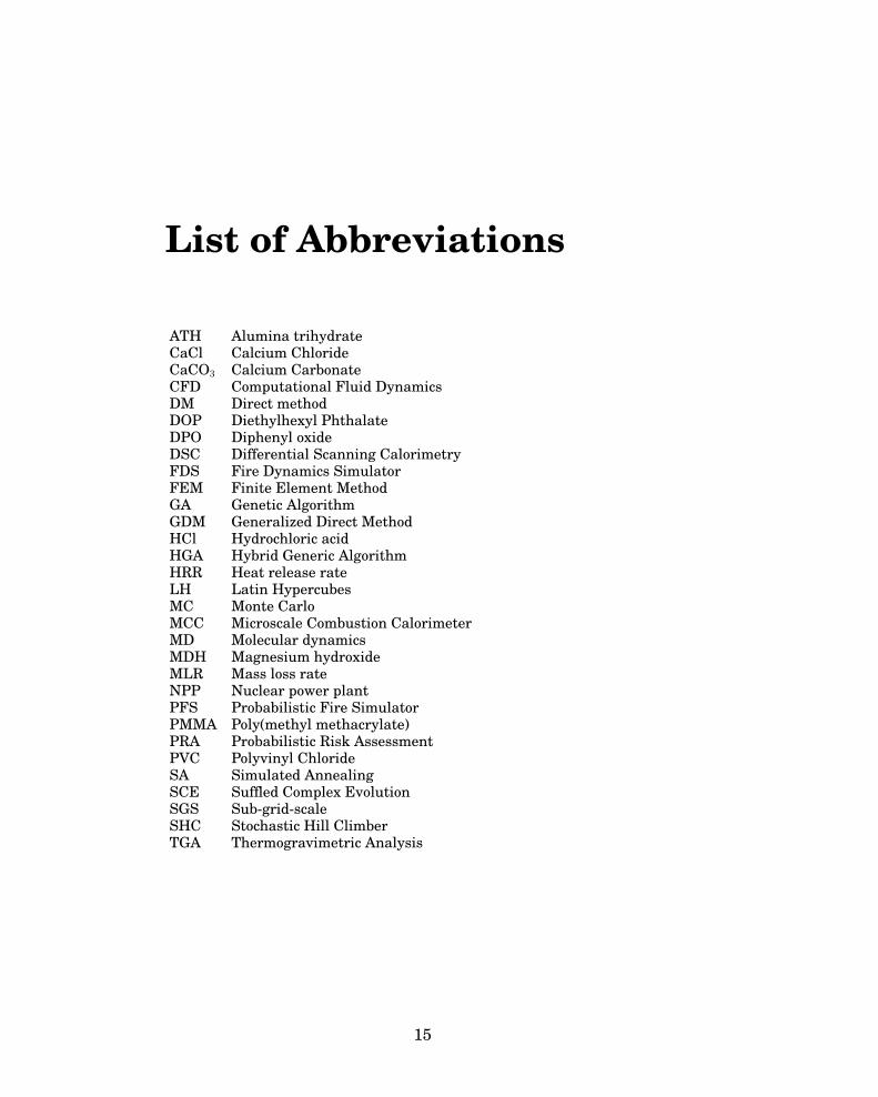
List of Abbreviations

ATH Alumina trihydrateCaCl Calcium ChlorideCaCO3 Calcium CarbonateCFD Computational Fluid DynamicsDM Direct methodDOP Diethylhexyl PhthalateDPO Diphenyl oxideDSC Differential Scanning CalorimetryFDS Fire Dynamics SimulatorFEM Finite Element MethodGA Genetic AlgorithmGDM Generalized Direct MethodHCl Hydrochloric acidHGA Hybrid Generic AlgorithmHRR Heat release rateLH Latin HypercubesMC Monte CarloMCC Microscale Combustion CalorimeterMD Molecular dynamicsMDH Magnesium hydroxideMLR Mass loss rateNPP Nuclear power plantPFS Probabilistic Fire SimulatorPMMA Poly(methyl methacrylate)PRA Probabilistic Risk AssessmentPVC Polyvinyl ChlorideSA Simulated AnnealingSCE Suffled Complex EvolutionSGS Sub-grid-scaleSHC Stochastic Hill ClimberTGA Thermogravimetric Analysis

15

1. Introduction

1.1 Background

Fire causes significant harm to people and property. In Finland, on average 100

people (about 18 per million citizens) die every year through fire, although thetrend has been descending in recent years. Deaths due to fires initiated fromsmoking or careless handling of fire decreased in 2007–2010, but the number offires caused by vandalism rose [1]. Although most fires that lead to death occurin residential buildings, the potential consequences of fire become especially se-rious in public places with high occupation yet limited evacuation possibilities,such as on aeroplanes [2] or ships [3]. Fires in industry may arise for variousreasons, including failing electronic components, dust, or vandalism, and causesignificant expenses to the owners and insurance companies.

In general, the objective of fire safety engineering is to protect first peopleand animals, then property and the fire fighters. In some safety critical facili-ties, such as nuclear power plants (NPP), these objectives are not enough: onemust also consider the environmental problems caused by leaking radioactivematerial or the economic losses of industry that are caused by the attendantlack of power. Fire at a nuclear power plant is considered to be among initiat-ing events (events that could begin a chain of events leading to a serious acci-dent) in probabilistic risk assessment (PRA); therefore it is a focus of extensiveresearch [4].

In the earlier times, building materials were limited to those available moredirectly from nature: wood, stone, and metals. Entire cities of wooden houseseasily burnt to the ground, and iron structures rust away and fall down. In the20th century, however, new materials started to emerge. The use of polymersand synthetic fibres increased in the manufacturing of furnitures and otherhousehold goods. As electronics grew more and more commonplace, kitchensand living rooms became filled with new gadgets and cables of various types.Cables also account for a significant proportion of the fire load at factories andpower plants.

The search for better materials led to the development of modern compos-ites. In transportation, the composites were designed to be lighter, less expen-sive, stiffer, or stronger than the original metal. These qualities make compos-ites very attractive, especially in, for example, the aviation industry. More than50% of the structure of an Airbus 380 is made of composite materials [5]. Unfor-tunately, the fire performance of these new materials does not always improve

16

Introduction

on (or even equal) that of the traditional materials. A laminate loses its struc-ture when heated, and in a polymer composite only parts of the material survivethe fire. A glass fibre reinforced phenolic composite after a fire is shown in Fig-ure 1.1. The structure is weakened by the pyrolysis of the phenolic polymer andthe subsequent delamination.

Clearly, the new materials needed protection from the heat. That is whyseveral flame retardant additives have been developed over the years. Somematerials are flame retardant by nature, such as charring wood or materialsthat release non-combustible gas that cools the surface and dilutes the com-bustion gases (as halogen in polyvinyl chloride (PVC) does). Halogenated flameretardants are not recommended nowadays, because of environmental concerns,but a similar mechanism has been adopted for new, non-corrosive flame retar-dants that release, for example, water [6, 7]. Wood charring has also inspirednew, intumescent surfaces that protect the underlying surface from the heat [8].

Figure 1.1. Glass fibre-Phenolic composite after fire.

Fire simulations are used extensively in the planning and design of new solu-tions for structures or interiors of buildings. They can be used as an elementof performance-based design, wherein the designer has to prove that the newsolution is at least as safe as the previously accepted solutions. They can alsobe used as part of the PRA of nuclear power plants [4].

Increased processing capacity and improvements to software have made ex-tensive fire simulations possible. The simulations can be used to predict firespread and/or its consequences and to study structural performance [9], the wa-ter suppression [10], evacuation safety [11], or even the human behaviour [12].Studies of the thermal degradation at atomic level have been done by means ofmolecular dynamics (MD) [13].

Pyrolysis modelling is an important part of a modern fire simulation. Tradi-tionally, the consequences of fire have been evaluated on basis of pre-described

17

Introduction

fires and standard fire curves. Pyrolysis modelling is designed to predict theheat release rate and the response of the structures and materials that follows.It allows implementation of more realistic fire scenarios and study of the flamespread.

In the future, pyrolysis modelling may also be used in product developmentfor new materials. Potential fire risks and the structures’ performance in firecould be evaluated by means of simulations before manufacture of large sam-ples. Pyrolysis modelling can also be part of the process of optimisation of thenew materials’ properties. This could be especially useful in development ofnew flame retardant materials or mechanisms.

Pyrolysis modelling consists of five steps:1. The material is tested experimentally on small scale. Typical experimental

methods in this connection are thermogravimetric analysis (TGA) [14,15] andcone calorimeter [16].

2. The experiments are described by a mathematical model. The pyrolysis isoften modelled by means of Arrhenius equation in combination with data onheat transfer [17,18]. The model’s validation is an important part of the pro-cess.

3. The model has to be solved numerically and this solution verified.4. Model parameters are often unknown and have to be estimated by fitting of

the model to the experimental results.5. The pyrolysis model is taken in combination with the computational fluid dy-

namics (CFD) calculations. This is the case with the Fire Dynamics Simulator(FDS) [18].

The present work concentrates on finding methods for estimation of the pyroly-sis parameters, an important topic since the model parameters are not alwayswell-known or even well-defined sets for any given material. They may varysignificantly, depending on the model’s limitations and complexity. Therefore,they cannot be listed in any handbook or on a product sheet. The most signif-icant difference between the work of a fire safety engineer and a product R&Dengineer is that the fire safety engineer does not usually have precise informa-tion about the fuel or fire load. There is a demand for methods that are accurateenough for predicting the material degradation correctly and at the same timeare simple and fast enough that they can be easily used by a practising fireengineer.

Several methods have been developed for extracting the reaction (or kinetic)parameters from the experimental data, some simple and fast and others morecomplicated but providing more accurate results. The other (thermal) param-eters are typically estimated from bench scale data [19] or in some cases mea-sured directly [20]. Publication I and Publication II cover the authors contri-

18

Introduction

bution to the estimation methods and Publication III describes the sensitivitystudy for the modelling choices.

This dissertation provides methods for pyrolysis modelling of these com-plex materials. It also offers methods for calculating the reaction specific heatrelease rate that can in some cases be used in estimation of the material com-position (in Publication IV).

Not only the material parameters, but also the geometry and structure, ad-ditives and flame retardants may cause challenges in larger scale simulationswith complex materials such as cables or composites. The methods are appliedto a real fire safety assessment for a nuclear power plant in Publication V.

The work on this dissertation was carried out primarily in two projects. Thematerial modelling of the cables for improving nuclear power plant fire safetyhas been developed as part of the Finnish Research Programme on NuclearPower Plant Safety (SAFIR 20101 and SAFIR 20142) [4]. The work pertainingto composites is done as part of the European Union project FIRE-RESIST3.

1.2 Outline of the dissertation

The dissertation is organised as follows:Chapter 2 provides the background on the work done for this dissertation.

First, the pyrolysis model and other important equations for the material mod-elling are reviewed. Then the experimental methods used for the parameterestimation are presented. Literature on some significant estimation methods isreviewed. Also, the Monte Carlo method is presented in brief.

Chapter 3 presents some special cases of pyrolysis modelling, includingthermoplastic and thermoset polymers and intumescent surfaces. It also pro-vides a literature review considering some complex materials (PVC, cables, andcomposites) and the associated modelling.

Chapter 4 summarises the methods developed by the author in the courseof the doctoral research. First, the FDS models of the experimental methodsare briefly described. After this, the applications of the two estimation methods(one analytical and one a curve fitting algorithm) are discussed, after which anapplication of new experimental method that can be used in parameter estima-tion, microscale combustion calorimetry (MCC), is presented.

Chapter 5 summarises the most important results emerging in Publica-tions I–V and some additional discussion related to the topics of this work.

Chapter 6 presents conclusions and discussion of the topic of the disserta-tion. Future plans and possibilities for applications are presented.

1See http://virtual.vtt.fi/virtual/safir2010/2See http://virtual.vtt.fi/virtual/safir2014/3See http://www.fire-resist.eu/FireResist/index.xhtml

19

2. Pyrolysis modelling and fire simulations

2.1 Motivation

If one is to be able to predict the spread of fire, the pyrolysis model, startingwith the solid phase degradation reactions, has to be defined. This chapter pro-vides background information and the literature survey needed for understand-ing of the concepts of pyrolysis modelling. First, a brief review of the pyrolysismodel and the equations needed for predicting the fire spread of a materialare presented. Then the experimental methods essential to the pyrolysis mod-elling are described. An review of literature on existing parameter estimationmethods is provided and discussed in brief. The methods applied and improvedupon for Publication I and Publication II are based on these methods. Lastly,the Monte Carlo simulation method is presented as it is relevant for an under-standing of Publication V.

2.2 The pyrolysis model

Pyrolysis is the thermal degradation that occurs in the solid phase of a mate-rial when it is heated. The bonds between the molecules start to break at ele-vated temperatures, leading to release of volatile compounds and changes fromthe original structure of the material. This is seen as mass loss. Technically,’pyrolysis’ refers only to thermal degradation without oxygen; in general (re-gardless of the oxygen concentration) the mechanism is called thermolysis. Inthe presence of air, the carbonous residue may oxidise. The combustible gasesreleased during the pyrolysis may also ignite, leading to combustion in the gasphase. This increases the gas temperature, with the results being slightly fasterdegradation than in inert ambient. In this dissertation, the term ’pyrolysis’ isused to describe the thermal degradation at elevated temperatures both in inertambient and in the presence of oxygen.

The temperature dependent reaction rate of the pyrolysis is often describedby the Arrhenius equation. This equation describes the temperature depen-dence of reaction constant

kr = Ae−ERT , (2.1)

where A is the pre-exponential factor, E the activation energy, R the universalgas constant, and T temperature. Originally developed by Svante Arrhenius

20

Pyrolysis modelling and fire simulations

in 1884 in study of the dissociation of electrolytes [21], the equation has beenapplied since then in various fields of research, from chemical and physicalprocesses to studies of quantum statistics and climate change [21–28]

In the fire community interest in the Arrhenius parameters grew in thelate 20th century, first for describing the char oxidation [29–31] and then forpredicting the thermal decomposition in the solid phase [17–19].

The equation gives a relationship between reaction rate and temperatureand is often represented in the form

rj =dα

dt= Ajf(α)e−

EjRT , (2.2)

where α = (m0 −m)/(m0) is the fractional conversion from reactants to prod-ucts ranging from 0 to 1, and T the temperature of the solid. The so calledkinetic triplet consists of Aj , Ej , and reaction model f(α). Each reaction j has adifferent kinetic triplet. The reaction model often depends on reaction order Nkand may be expressed as

f(α) = (1− α)Nj . (2.3)

The stoichiometric reaction orders of chemical reactions are integers (usually1). The thermal degradation is a consequence of the chemical bonds breaking atelevated temperatures. The materials consist of several, different bonds, requir-ing different amounts of energy for breaking. The overall mass loss reaction is,therefore, a combination of several chemical reactions. In pyrolysis modelling,these reactions are lumped together and hence fractional reaction rates also areused. The model is not an attempt to describe each chemical reaction exactly;the parameters should be considered model specific elements that merge thenet effect of several overlapping reactions.

The reaction rate depends on the temperature. The temperature at thefront surface of the material rises through by radiation and convection, whileinside the material the heat is transferred via conduction and internal radia-tion. A one dimensional heat conduction equation with internal heat genera-tion/absorption is often sufficient to determine the temperature gradient, T (x):

ρcpdT

dt=

∂

∂xk∂T

∂x+ q

′′′

s , (2.4)

where ρ is the solid density, cp the specific heat capacity, k thermal conductivity,x depth from the surface and q

′′′

s a source term that consists of the chemicalreactions (q

′′′

s,c) and the radiation and emission at depth (q′′′

s,r). The chemical

21


source term is linked to the Arrhenius equation by the reaction rate:

q′′′

s,c = −ρ0

∑

j

rj(x)∆Hj , (2.5)

where ∆Hj is the heat of reaction of reaction j.The boundary condition at front (F ) surface is

−k ∂T∂x

(0, t) = q′′

c + q′′

r , (2.6)

where convective heat flux q′′

c is

q′′

c = h(Tg − TF ); (2.7)

constant h is the heat transfer coefficient, and the net radiative flux is

q′′

r = q′′

r,in − ε σ T 4F , (2.8)

where ε is the emissivity and σ the Stefan-Boltzmann coefficient. [14,18]In the presence of air, the combustible gases released during pyrolysis may

ignite and lead to combustion. This is modelled through assumption of a com-ponent specific heat of combustion (∆Hc) that describes the heat released perunit mass. The heat release rate per unit area then becomes

q′′

= m′′∆Hc = ∆Hc

∫ L

0

∑

j

∑

i

Ai,jρie−Ei,j/RT (x)dx, (2.9)

where i is the component (material) index and j reaction index.Materials that can sustain smouldering combustion are porous and form

solid carbonaceous char when heated. Materials that melt do not exhibit thiskind of combustion. The char is formed on the exposed surface. When the charis oxidised in this region, a glow at high temperatures (about 600◦C for wood) re-sults. This exothermic process yields ash and residual char, along with volatileproducts (e.g., tar) that have high carbon monoxide content. These products arealso flammable if accumulating in a closed space; hence, smouldering may leadto flaming after passage of considerable time. [14]

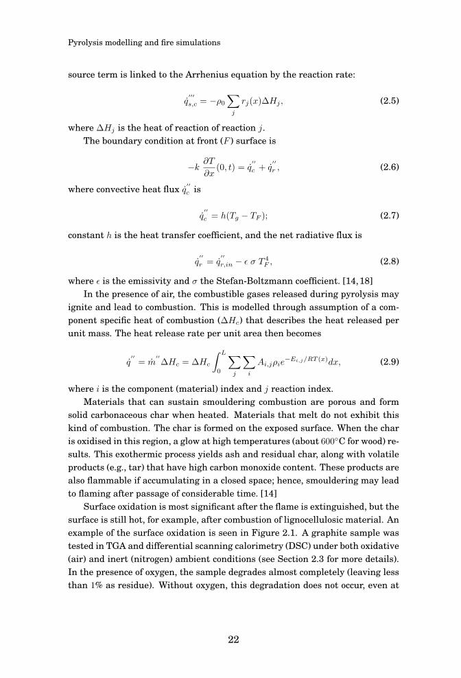
Surface oxidation is most significant after the flame is extinguished, but thesurface is still hot, for example, after combustion of lignocellulosic material. Anexample of the surface oxidation is seen in Figure 2.1. A graphite sample wastested in TGA and differential scanning calorimetry (DSC) under both oxidative(air) and inert (nitrogen) ambient conditions (see Section 2.3 for more details).In the presence of oxygen, the sample degrades almost completely (leaving lessthan 1% as residue). Without oxygen, this degradation does not occur, even at

22


high temperatures and with a slow heating rate. Similarly, the DSC experi-ments show a clear exothermic reaction peak for the sample in air, while thesame test in nitrogen does not show any reaction (except minor experimentalfluctuation of the baseline).

0 200 400 600 800 1000 12000

20

40

60

80

100

120

Temperature (°C)

TGA

(%)

In airIn N2

0 200 400 600 800 1000 1200−1

0

1

2

3

4

5

Temperature (°C)

DSC

(mW

/mg)

In airIn N2

a) b)

Figure 2.1. a) TGA and b) DSC experiments with graphite in air and in nitrogen at2 K/min.

A reaction depending on the oxygen concentration can be modelled by means ofa modified Arrhenius equation:

rO2,j = Aj(1− αj)Nj exp

(− EjRT

)YNO2

O2, (2.10)

where YO2is the oxygen concentration and NO2

is the reaction order of theoxygen concentration. If reaction rate does not depend on oxygen concentration(as normal pyrolysis reaction), NO2 = 0.

The material in the model consists of several pseudo-components. A pseudo-component (later also simply component) refers to a component in the modelthat represents one mass loss step in the model. It does not necessarily repre-sent any particular chemical reaction, but it does serve as a way to model thenet effect of all reactions occurring simultaneously. In total, there are at least10 model parameters per reaction or component. Each component is describedin terms of these parameters. Some components may encompass several reac-tions (or competing reactions), which increase the number of parameters stillfurther. The parameters in the model are summarised in Table 2.1.Several pieces of software have been developed in the fire community for mod-elling the thermal degradation of solids: FDS1 [18], Gpyro2 [19], Open Foam3,and ThermaKin [32]. FDS and OpenFoam are CFD codes while Gpyro and

1See https://code.google.com/p/fds-smv/2See http://code.google.com/p/gpyro/3See http://www.openfoam.com/

23


Table 2.1. Summary of parameters of pyrolysis modelling. Est estimated from and Mesmeasured with. (R) reaction specific. (C) component specific.

Param. Explanation Eq. Method of obtaining Reaction/(unit) Component

A Pre-exponential 2.2 Est TGA/MCC Rfactor (s−1)

cp Specific heat 2.4 Mes DSC / C(kJ/(K·kg)) Est cone calorimeter

E Activation energy 2.2 Est TGA/MCC R(J/mol)

∆H Heat of reaction 2.5 Mes DSC / R(kJ/kg) Est cone calorimeter

∆Hc Heat of combustion 2.9 Mes MCC / R(kJ/kg) / (MJ/kg) Est cone calorimeter

k Thermal conductivity 2.4 Mes / C(W/(m· K)) Est cone calorimeter

N Reaction order 2.2 Est TGA/MCC RNO2 Reaction order 2.10 Est TGA results in air R

of oxidationε Emissivity 2.8 Est cone calorimeter Cρ Density 2.4 Meas directly C

(kg/m3)

ThermaKin are limited to the solid phase. Gpyro also includes an algorithm forestimation of the model’s parameters.

2.3 Experimental methods

The experiments commonly employed in fire research can be divided into small(milligram), bench (gram to kilogram), and large/full (kilogram to metric ton)scale experiments on the basis of the sample size required. The small scale ex-periments are the easiest to model and involve less inaccuracy related to fireor experimental set up. The material models are typically built on the basis ofsmall and bench scale experiments. Large scale fire tests are often very expen-sive, but important for code validation purposes.

2.3.1 Small scale experiments

In a small scale experiment, the sample mass is usually 1–30 mg. These ex-periments typically measure only one property at a time, such as mass, heat ofreaction, specific heat, or heat release rate. The reaction parameters and some-times even a good estimate as to the sample composition can be determined bymeans of small scale experimental results.

24


The most commonly used small scale experiment for pyrolysis modelling isthe TGA. It uses a small furnace filled with either air or inert purge gas (of-ten nitrogen). The sample is inside a small crucible that is placed over a loadcell. During the experiment, the sample mass is measured. The experimentcan be performed either isothermally (i.e., at a one constant temperature) ornon-isothermally (with temperature increasing linearly). The non-isothermalexperiment is often more suitable for the estimation of the pyrolysis parame-ters, since it also provides information about the reaction temperatures. Theheating rates are relatively low (2–30 K/min), in order to keep the sample inthermal equilibrium with the furnace. [14,15] For pyrolysis modelling purposes,TGA experiments are often performed at several heating rates. This is neces-sary, because the chemical reactions may depend on heating rate, and usingseveral rates enables the estimation of more general reaction parameters. Anexample of TGA results at several heating rates is seen in Figure 2.2. Often theincreasing heating rate moves the reaction to higher temperatures. That meansthat the reaction takes place more slowly than the heating of the sample andtherefore the temperature of the sample is higher when the mass loss occurs.At very high heating rates or with thermally thick samples the thermal equilib-rium between the furnace and sample may be lost and the sample temperatureno longer corresponds to the furnace temperature.

100 200 300 400 500 600 70010

20

30

40

50

60

70

80

90

100

Mas

s (%

)

Temperature (°C)

2 K/min5 K/min10 K/min20 K/min

Figure 2.2. TGA results of birch wood at 2–20 K/min heating rates in nitrogen ambient.

25


More information about the reaction enthalpies and specific heat is provided byanother small scale experiment, DSC. The furnace and the method of operationare similar those in TGA. In DSC, the sample temperature is regulated relativeto a reference sample, and the required energy is measured. With DSC, onecan perform experimental measurements in an individual experiment or simul-taneously with TGA. From individually measured DSC, one can calculate theheat of reaction and the specific heat capacity. It is good to keep in mind thatthe measured value is actually the joint effect of possibly several simultaneousreactions. The results should then be scaled for the target application, morespecifically, to its reaction path. [14, 15] For accurate calculation of the specificheat, three measurements are required in all: of the actual material, of a ref-erence sample with known specific heat (often sapphire), and of an empty panfor setting of the baseline. The baseline value is subtracted from the results forthe actual sample and the reference. The specific heat capacity of the referencesample is scaled by the ratio of the DSC measurements between the sample andthe reference:

cp,s(T ) =qs/ms(T )

qr/mr(T )cp,r(T ), (2.11)

where the subscript r refers to the reference and s to the sample.A simpler but less accurate method is to calculate the specific heat by using

only the baseline corrected heat flow of the sample. Then the heat flow for theinitial mass is scaled by the current heating rate β:

cp,s =qs/ms

β. (2.12)

A comparison of the results of these methods is shown in Figure 2.3.The heat of reaction (or reaction enthalpy) is calculated as the integral over thereaction peak in DSC. An example of the definition of the heat of reaction isseen in Figure 2.4.

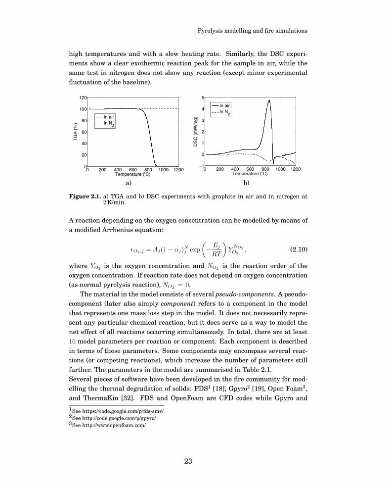
When DSC is performed simultaneously with a TGA experiment, the re-sults are mostly more qualitative than quantitative. Often a significant, un-predictably behaving baseline can be observed in the simultaneous DSC resultsthat make the calculation of reaction enthalpy extremely difficult. This is prob-ably because of experimental uncertainty that comes from the set-up necessaryfor measuring the sample mass simultaneously with the heat flow. Qualitativeresults may, however, be very useful, since they reveal whether the reaction isendothermic or exothermic. In Figure 2.5, qualitative DSC results for heat flowin nitrogen and in air can be seen. Three reactions can be observed in air, twoin nitrogen. The first one occurs at around 100◦C and is endothermic in bothpurge gas conditions. An endothermic reaction that occurs at low temperature

26


T (°C)

c p (kJ

/K⋅m

)

Direct method

Sapphire method

0.25

Figure 2.3. Comparison of direct method to sapphire method in calculation of specificheat from DSC results for a furane sample. Experimental data courtesy ofGaiker.

250 300 350 400 4500.2

0.3

0.4

0.5

0.6

0.7

0.8

0.9

1

1.1

1.2

T (°C)

DS

C (

mW

/mg)

∆H

Figure 2.4. Integration over the reaction peak for determination of the heat of reaction.

can usually be identified as evaporation of moisture. The second reaction takesplace after 300◦C and is exothermic in air and endothermic in nitrogen. The ad-ditional reaction only in air (peak at 440◦C) is defined as char oxidation. In the

27


presence of air, the exothermic peaks can indicate oxidative surface reactionsor flaming combustion. It is difficult to know for certain if the combustion gasesare ignited during the test or not, although self-ignition is not very probableat low temperatures. The possibility of ignition can be decreased by reducingsample size.

0 200 400 600 800−2

0

2

4

6

8

10

12

T (°C)

DS

C (

mW

/mg)

AirN

2

Figure 2.5. DSC results for birch at 10 K/min in air and nitrogen. Exothermic peaks arepositive.

Microscale combustion calorimetry (MCC) can be used for measuring the heatrelease rate of a sample. It first pyrolyses the sample in a nitrogen environment,at a higher heating rate than in the TGA (typically around 60 K/min, althoughheating rates from 12 to 120 K/min are possible). Then the pyrolysis gases flowinto a combustor, a tube whose high temperature and sufficient oxygen concen-tration cause all the combustible gases to burn immediately. The result is theheat of complete combustion as a function of temperature. [33, 34] The pyroly-sis can alternatively be done in air, to study the oxidation of pyrolysis char. Inthis work, the MCC results are combined with the information from the TGAfor determination of the heat of combustion values for each reaction. This in-formation can be used when one is simulating complex materials, e.g., polymersamples. [35]

28


2.3.2 Bench-scale tools – the cone calorimeter

The cone calorimeter (ISO 5660-1, [16]) is the most commonly used bench-scaleexperimental tool in fire research. The sample usually has dimensions of 10 cm× 10 cm× 0.1–5 cm and has a substrate made of mineral-based insulation or cal-cium silicate board on the unexposed surface. The sample is placed under a coneshaped heater, which heats the sample with a radiant heat flux of 10–75 kW/m2.The igniter is an electric spark that is kept on until the sample ignites, al-though spontaneous ignition may also be investigated without use of the sparkigniter. The gases are collected in a hood, from which the various properties aremeasured. As a result, the cone calorimeter provides information about massloss, heat release rate, and soot yield. Additionally, sample temperatures maybe measured by means of thermocouples. The standard cone calorimeter oper-ates in ambient air, but ambient controlled cone calorimeters are available also.They can be used for studying the effect of the oxygen in the atmosphere or thepyrolysis of the sample in an inert (nitrogen) ambient. [16,36,37]

2.4 Parameter estimation

The reaction rate of the thermal degradation of a material is often modelled bymeans of Arrhenius equation as explained in Section 2.2. The kinetic param-eters cannot be measured directly; they need to be estimated somehow fromthe experimental data. An overview of methods to quantify kinetic parametersis provided in the following sections. The estimation algorithms presented inSubsection 2.4.2 can also be used in estimation of other (mainly thermal) modelparameters.

2.4.1 Semi-analytical methods

The first methods, developed in the 1960s, included approximations, referencepoints, and graphical solutions [38–40]. The isoconversional (i.e. applying mul-tiple heating rates) methods were soon discovered to be more useful becausethey provide more general results. They can be used for defining the reactionmodel (f(α)) or the reaction parameters (A, E) [22–25]. Drawbacks to theseanalytical methods may be found in their limited accuracy; inconvenience oflocating various reference points; limitations in reaction steps or order; or, insome cases, the fact that the complete kinetic triplet, (A, E) or f(α), cannot besolved from the same data set. The fire community’s interest in the reaction pa-rameters has led to some new, simple but reasonably accurate methods, aimedat encouraging modellers to base their kinetic parameters for their material

29


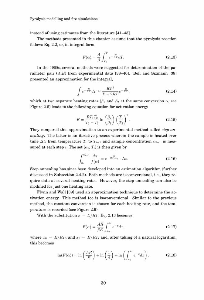
instead of using estimates from the literature [41–43].The methods presented in this chapter assume that the pyrolysis reaction

follows Eq. 2.2, or, in integral form,

F (α) =A

β

∫ T

T0

e−ERT dT. (2.13)

In the 1960s, several methods were suggested for determination of the pa-rameter pair (A,E) from experimental data [38–40]. Bell and Sizmann [38]presented an approximation for the integral,

∫e−

ERT dT ≈ RT 2

E + 2RTe−

ERT , (2.14)

which at two separate heating rates (β1 and β2 at the same conversion α, seeFigure 2.6) leads to the following equation for activation energy

E =RT1T2

T2 − T1ln

(β2

β1

)(T1

T2

)2

. (2.15)

They compared this approximation to an experimental method called step an-nealing. The latter is an iterative process wherein the sample is heated overtime ∆ti from temperature Ti to Ti+1 and sample concentration αi+1 is mea-sured at each step i. The set (αi, Ti) is then given by

∫ αi+1

αi

dα

f(α)= e− ERTi+1 ·∆t. (2.16)

Step annealing has since been developed into an estimation algorithm (furtherdiscussed in Subsection 2.4.2). Both methods are isoconversional, i.e., they re-quire data at several heating rates. However, the step annealing can also bemodified for just one heating rate.

Flynn and Wall [39] used an approximation technique to determine the ac-tivation energy. This method too is isoconversional. Similar to the previousmethod, the constant conversion is chosen for each heating rate, and the tem-perature is recorded (see Figure 2.6).

With the substitution x = E/RT , Eq. 2.13 becomes

F (α) =AR

βE

∫ xi

x0

e−xdx, (2.17)

where x0 = E/RT0 and xi = E/RTi and, after taking of a natural logarithm,this becomes

ln(F (α)) = ln

(AR

E

)+ ln

(1

β

)+ ln

(∫ xi

x0

e−xdx

). (2.18)

30


The above-mentioned authors found that for E/RT ≥ 20, the integral can beapproximated thus:

ln

(∫ Ti

T0

e−ERT

)dT ≈ −2.315− 0.457

E

RTi(2.19)

and therefore E becomes, after differentiation,

E ≈ − R

0.457

∆ ln(β)

∆T−1. (2.20)

This approximated value is then used for calculation of a more accurate esti-mate for E/RT and consequently its integral. This method was developed in atime when solving integrals numerically was not commonly performed. Instead,approximations and lists of integral values were used.

440 460 480 500 520 540 5600.6

0.65

0.7

0.75

0.8

0.85

0.9

0.95

1

T (K)

1−α

β1

β2

β3

T1

T2

T3

Figure 2.6. Demonstration of selecting different reference points for Flynn’s isoconver-sional method.

Friedman [40] suggested several methods that are based on reference pointsand allow the use of reaction orders that are not equal to one. His methodsare based on either reference points from two heating rates, or multiple pointsfrom the same data. In the simplest form, the reference point is chosen from

31


the point of the highest reaction rate ( d2αdT 2 = 0):

E = NRT 2p

( dαdT )p

1− αp. (2.21)

Another relation, a slightly more elaborate one, requires two reference pointsfor the same heating rate

E = −Rln

(( dαdT )

2

( dαdT )1

)+N ln

(1−α1

1−α2

)

T−12 − T−1

1

. (2.22)

Friedman also provided several relations for reaction order N that shall be dis-cussed later in this section.

Since the 1980s, an isoconversional method that is based on linear fitting hasbeen widely used in many fields of research in slightly different forms [22–25].Methods in this family are also called the model-free methods, because they donot require an analytical form of the reaction model (f(α)). The approach can beapplied either for isothermal thermogravimetric data at several temperaturesor to non-isothermal data at one heating rate.

The idea of the isothermal version is to take the natural logarithm of bothsides of the Arrhenius equation. After rearrangement of the terms, it becomes

ln

((dαdT

)

f(α)

)= ln(A)− E

RT. (2.23)

The left-hand side of the equation consists of the experimental values thatshould form a line when plotted against T−1 with ln(A) being the intercept and-E/R the slope. If f(α) depends on N , the best fit can be found through repeat-ing of the calculation at several reaction orders, and the best fitting solutionwill be chosen. [22,23]

In non-isothermal conditions, the above-mentioned method becomes a bitmore complicated. If the measurement is done at only one heating rate, theresults are often ambiguous. Keuleer et al. [23] suggest using the equation

ln

(β(dαdT

)

f(α)

)= ln(A)− E

RT(2.24)

at several heating rates (β) at fixed values of conversion α. Liu et al. [25] basetheir method on an approximation of the temperature integral yielding the lin-ear relationship

ln

(β

T 2

)= ln

(AR

Eg(α)

)− E

RT, (2.25)

32


where g(α) =∫ α

0dαf(α) = AE

βR p(ERT ).

Other related methods have been suggested and presented by several au-thors over the past few years [21,24,44–47].

The key parameter of f(α) for the reaction order model is the reaction orderN . From the chemistry point of view for thermal degradation reactions reactionorders other than 1 do not have real meaning, as is discussed in Section 2.2.Many simplified reaction models are limited to the first order. However, the re-action order does affect the reaction rate shape significantly, so it is often usedin modelling when the effects of several simultaneous reactions are approxi-mated with just one kinetic reaction.

Friedman [40] presented several equations for calculation of N . The follow-ing equation is based on three well-separated reference points from the samedata

N =ln(

( dαdT )3

( dαdT )1

)− T2(T3−T1)

T3(T2−T1) · ln(

( dαdT )2

( dαdT )1

)

T2(T3−T1)T3(T2−T1) · ln

(1−α1

1−α2

)− ln

(1−α1

1−α3

) (2.26)

This method works very well for smooth data and non-overlapping reactionsbut may be complicated for real data, as discussed in Publication II.

Gao [48] has provided a more practical approach by listing theoretical limitsfor the reaction order as a function of the conversion. Through a polynomialcurve fit, those values convert into a very simple relationship (as demonstratedin Publication II):

N ≈ 13.25(1− α∗p)3 − 4.16(1− α∗p)2 + 2.3(1− α∗p)− 0.077, (2.27)

where α∗p is the reaction progress variable at the peak of the reaction.The isoconversional method provides also a good way of defining N . Li and

Järvelä [24] suggest that the reaction rate can be expressed as

r =(dαdt )

(1− α)N. (2.28)

After one takes a natural logarithm and rearranges this, it results in

ln

(dα

dt

)= ln(r) +N ln(1− α). (2.29)

If ln(dα/dt) is now plotted against ln(1−α) at several temperatures, the N valueis equal to the average slope of these lines.

33


2.4.2 Optimization algorithms

The analytical methods solve the parameters by using reference points, and theresults depend only on the choice of method and the location of the referencepoint. Another approach is to consider the parameter estimation as an optimi-sation problem wherein the model is fitted to the experimental data. Severalcurve-fitting algorithms have been developed over the years. The traditionalgradient methods tend to converge at the closest local minimum (not necessar-ily the global optimum) and therefore generally do not operate well with thiskind of problem. Accordingly, evolutionary algorithms were considered. Thefirst attempts used genetic algorithms (GA) [17, 19, 31]. These do operate veryefficiently for non-linear problems with a large number of unknown parameters.However, GAs may be utterly inefficient with large estimation boundaries andtherefore require several iterations and large sets of candidate solutions. Sev-eral other algorithms have been studied and successfully used in estimation ofthe pyrolysis parameters [49–53]. All of these methods require purpose-specificsoftware and significant computation time, and their stochastic nature meansthat the estimation procedure cannot be repeated exactly. The results also de-pend on the estimation boundaries and algorithm parameters defined by theuser. However, the above mentioned shortcomings are compensated by the al-gorithms’ advantage of not being limited to any specific model. Besides thepyrolysis kinetics, a GA can be used in estimation of any other parameters. Inthe fire sciences, these other parameters would typically be the thermal param-eters as listed in Table 2.1.

The idea of GA [17, 19, 31] is based on the evolution and survival of thefittest. Each set of parameters represents one individual in a population. Theindividuals consist of parameters – or genes, as they are called in GA argot.The first population is selected randomly from the pre-defined range. The in-dividuals are located in several subpopulations that do not share the genes innormal routines. Each individual is tested against the experimental data, anda value called the fitness value is calculated for measuring the goodness of thefit. The population goes through a set of operations that are stochastic, andtheir probabilities depend on the fitness value. These operations include selec-tion (selecting the best-fitting solutions for reproduction), cross-over (combiningtwo selected individuals for production of a new individual, offspring), mutation(changing one or more genes of some individuals into a random number), andmigration (migrating, on the part of individuals, between subpopulations). Thenext generation consists of the best fitting individuals of the previous genera-tion and of the new offspring. The operations based on the fitness value andprobabilities cause the population converge towards the best fitting solutions,

34


and the mutation and the migration bring new genes to the subpopulations andhence prevent convergence at a local minimum. A flowchart of the algorithmis shown in Figure 2.7. This topic is further discussed in Subsection 4.4.2 andin Publication I.

Choice of estimation boundaries and algorithm parameters.

Creation of initial (random) population or use of initial values

Calculate fitness value

Ranking Selection

Reproduction

Mutation (of offspring)

Calculate fitness value (offspring)

Replace (some) parents with offspring

Migrate Is ending condition fulfilled?

YesNo Algorithm ends

Figure 2.7. Flowchart of a genetic algorithm.

Shuffled complex evolution (SCE) is, in essence, an improved genetic al-gorithm [49, 54]. It starts similarly, with a random population, but is betterorganised and optimised with respect to the following operations. First, the in-dividuals are ordered according to their fitness values. Then they are dividedinto complexes such that every nth individual is placed in the same group. Ev-ery individual within a complex, a probability then is assigned that determineswhich q individuals are to be selected for a subcomplex. The values are orderedby their fitness values. The worst fitting value (uq) in the subcomplex is com-pared to other values within the group and a new value is calculated as

r =2

1− q

1−q∑

j=1

−uq. (2.30)

If r is not within the estimation boundaries, a new random value is gener-ated instead. If the fitness value of the new value is smaller than previously

35


(fr < fq), the new value r replaces the old value uq. Otherwise, a new value iscalculated, as

c =

11−q

∑q−1j=1 +uq

2. (2.31)

Comparison of the fitness values is performed as before. This operation is re-peated within the subcomplex until the predetermined number of iterations arecompleted. After that, the same operations are performed for each of the othersubcomplexes. When all the subcomplexes have been gone through, the conver-gence condition is checked. If this has been satisfied, the algorithm ends. If not,it starts running again from the sorting of the fitness values and distribution ofcandidate solutions to complexes.

This method has been applied to estimation of the parameters related tothermal degradation of several materials by Chaos et al. [49] and Lautenbergerand Fernandez-Pello [50]. The SCE approach has proved to be more efficientand to provide more accurate results than GAs do.

Hybrid genetic algorithms (HGA) combine the evolutionary algorithmand local search methods (e.g., gradient methods) [52, 55–57]. They have beendeveloped to enhance the algorithm such that it produces higher quality solu-tions more efficiently. The local search method can be included in any of threephases in the estimation process: before, during, or after the algorithm. Beforethe GA operation (pre-hybridisation), the local search is used for generating theinitial population for the GA and therefore reducing the solution space. Thisis suitable for some specific problems but not in general. The second option,which some refer to as organic hybridization, is used as one more operator forthe GA, improving the fit of each individual in each generation. Although thisis computationally more efficient than a GA alone, there is no guarantee of find-ing the global optimum. The last method is referred to as post-hybridisation.Here a GA is used to provide the initial design for the local search method. Thishas proved to be generally the most efficient way to hybridise the GA, since theglobal and local searches are performed completely separately.

Saha et al. [52] have successfully applied HGA for estimation of the kineticparameters of various plastics. They used the post-hybridisation technique anda multidimensional, unconstrained non-linear search function as a hybrid func-tion.

Stochastic hill climber (SHC) algorithm was developed by Webster [53]for his master’s thesis in 2009. The algorithm differs from GAs in the followingrespects:• The initial population is generated via good engineering judgement (or by

rules of thumb, discussed in Subsection 4.4.3). Webster has stated that it

36


is more logical to start with a well-fitting curve that has ’wrong’ parametersthan with a non-fitting curve that has the ’right’ parameters.• The fitness function involves an R-squared value.• Reproduction is done via mutation only (i.e. with no cross-breeding). The

parents may outlive the children if they have better fit.• The mutation magnitude of each parameter is limited such that each can

effect no more than 5% change in accuracy. This is done in order to preventany single parameter from dominating in the estimation process.• The mutation magnitude is multiplied by a scalar that depends on the muta-

tion history of the parameter. If the previous mutation attempts have beensuccessful, the scalar has a higher value than if the mutations have been un-successful.

This method has been applied to the estimation of cone calorimeter resultsby Webster himself, and by Lautenberger and Fernandez-Pello [50], with goodresults.

Simulated annealing (SA) differs from the previously presented algo-rithms in not being an evolutionary algorithm. It is, however, based on a real-life process – namely, annealing in metallurgy. In annealing, the material isfirst heated and then cooled, for finding of lower internal energies. In the al-gorithm, the initial solution is tested against a random solution. The choice ofsolution is based on the difference in fits and a random number that dependson a parameter referred to as temperature. The temperature is eventually de-creased, and the probability of choosing the worse-fitting solution decreaseswith it [51, 58, 59]. Mani et al. [51] applied SA for estimating the kinetic pa-rameters of lignin with good results.

Lautenberger and Fernandez-Pello [50] compared the performance of fouralgorithms (a GA, SCE, SHC, and a hybrid of a GA and SA). They tested theseestimation methods by using generic cone calorimeter data, so that the realtarget values of the parameters were known. They evaluated the algorithmsin terms of their effectiveness and robustness. The most rapid convergencewas shown by SHC, but the final fitness was at a level similar to that with GAand HGA, and SCE turned out to perform with the best fit with any randominitial population. These solutions were practically independent for the initialpopulation, and it seems that SCE is able to find an actual global optimum forthe problem. When the target values of the parameters were compared, thevalues estimated via SCE were the most accurate by far. The other algorithmswere much less accurate with respect to correctness of the target values, withHGA producing the greatest accuracy of the three while SHC showed the leastaccurate fit.

37


2.4.3 The compensation effect

As is discussed above, the values for the activation energy may be very sensitiveto small changes in experimental conditions (such as heating rate); therefore,isoconversional methods are commonly used, preferred over a single heatingrate experiments. This phenomenon is also widely recognised in the litera-ture [25, 60, 61] and observed in experiments, but no comprehensive explana-tion has been provided so far. There are two main, and opposite, points of viewon the nature of the compensation effect; it either is caused by an experimen-tal artefact or has a true chemical meaning. The second case is often seen asdiscomforting, since it means that the A and E values are not independent andtherefore do not have any physical meaning in isolation. In fire modelling, theinterpretation has been that the compensation effect has a chemical meaning.

The general form of the compensation effect is

ln(A) = a+ bE, (2.32)

where a can be very small [60, 61]. The analytical form of the compensationeffect is, according to Nikolaev et al. [60],

ln(A) = ln

(Eβ

RT 2p

)+

E

RTp. (2.33)

Slightly different form for the compensation effect has been suggested by Lyonand Safronava [62]:

ln(A) = ln

(βE

φRT 2p

)+

1

RTpE, (2.34)

where φ = −df(α)/dα. The compensation effect depends on rate and model, asobserved.

Similar behaviour has been observed more generally with other model pa-rameters, especially with larger-scale models. The models inevitably have somedegree of inaccuracy, and the parameters combine to form a model that fits toexperiments. Therefore, the model parameters actually work together to com-pensate for the shortcomings of the model and several combinations, fittingequally well, can be found for the same experimental data. This phenomenonis demonstrated and discussed in Publication III. However, good initial guesses(e.g., by model-free methods) may help to eliminate the randomness of the solu-tions and keep the parameters more realistic [63].

38


2.5 The Monte Carlo technique

Fire modelling can be used as a part of PRA. The goal of fire-PRA is to deter-mine the probability of the various possible consequences of a fire and discoverthe most significant parameters that correlate with the most severe conditions.The Monte Carlo (MC) technique is a tool for the statistical assessment. Thismethod is not used for parameter estimation as the methods described previ-ously in Section 2.4. In this dissertation, it has been used to statistically studyfire spread from one cable tray to another, as described in Publication V.

The Monte Carlo technique in its simplest form means repeating an actionseveral times at a random points in a parameter space and counting the events.A simple example of this technique is a game of tossing a coin to estimate theprobability of heads or tails. The modern Monte Carlo was born in the 1940swhen Stanislaw Ulam, John von Neumann, and others, started to use randomnumbers in the calculations of statistical physics. The most efficient use of theMC technique is to determine definite integrals that are too complex to solveanalytically. [64,65]

In applications of Monte Carlo for fire research, a simulation is repeatedseveral times, using random numbers from certain distributions of input pa-rameters. The number of repetitions should be high enough to cover the vari-able space for capturing the statistics of the events. This is computationallyquite expensive, so a more optimised sampling method is used. The samplingmethod, called Latin hypercubes (LH), is a type of stratified sampling. The ideais to divide the range of each variable into as many intervals as the number ofsamples so that each interval has equal probability according to the distribu-tion. From each interval, one random number is selected, and the random num-bers of each parameter are paired in a random manner. As its result the samplerepresents the space of possible input values more extensively than traditionalrandom sampling does, and, therefore, fewer repetitions are required. [66,67]

For fire Monte Carlo, a software package called Probabilistic Fire Simulator(PFS) is used. It was developed at VTT Technical Research Centre of Finland.It runs Monte Carlo (or two-model Monte Carlo) with a chosen fire model, mostcommonly with FDS [68, 69]. This tool has been used in the simulations de-scribed in Publication V.

39

3. Materials

3.1 Motivation

The thermal degradation process depends on the material. The degradationvaries with the polymer classes, whether the surface swells or shrinks whenheated and what kinds of flame retardants, if any, are used. A brief literaturesurvey is presented that considers these processes. Special attention is given tocomplex but very important materials: cables and composites. The challengesand the solutions from a modelling point of view are discussed in Section 3.5.

3.2 Thermoset and thermoplastic polymers

Synthetic polymers are classified as thermoplastic or thermoset by their be-haviour when heated. When exposed to heat, thermoplastic polymers softenand melt, and they take a new form when cooled down. This may affect theirburning through forming of falling droplets or burning liquid pools. Thermosetpolymers, on the other hand, are cross-linked structures that do not melt whenheated; they often leave residual char. Of the natural polymers, cellulose is sim-ilar in fire behaviour compared to synthetic thermoplastic polymers. A thirdpolymer class would be the elastomers, which can be distinguished by theirrubber-like properties. They can behave either like thermosets or as thermo-plastics do, depending on the material. [14,70]

3.3 Modelling shrinking and swelling surfaces

A solid surface seldom maintains its structure when exposed to heat. If a ho-mogeneous material is converted completely to volatiles, the material thicknessdecreases as the fire progresses. However, many materials do not degrade com-pletely and instead leave empty spaces (porosity) in the structure. Some gasfrom the pores may get trapped under the surface, causing the material to swell.This mechanism acts as a natural flame retardant for many charring materials,and the idea has been adopted for several synthetic flame retardants as well.More about the swelling (or intumescent) surfaces as a flame retardancy mech-anism is explained in Section 3.4. Many charring materials (e.g., wood) firstswell in the charring phase, and later shrink (in the presence of oxygen) whenthe char oxidises.

Shrinking and swelling have a significant effect on the thermal degrada-

40

Materials

tion of a material. Increasing porosity decreases the thermal conductivity, anda swollen surface forms a physical barrier to the heat. The simplest way tomodel this is to calculate the final thickness by using the information aboutresidue fraction and final density. One can calculate the density that the ma-terial would have after the reaction if the thickness were to remain unchanged(ρs,i). If the final density (ρi) is defined to be higher than the one calculated,the material shrinks; if lower, the material swells. In FDS version 6 [71], thisis done by decreasing or increasing the solid cell size in keeping with the ratioof the densities:

δ =

maxi

(ρs,iρi

)if maxi

(ρs,iρi

)≥ 1

∑i

(ρs,iρi

)if maxi

(ρs,iρi

)< 1.

(3.1)

The cell thickness is then scaled by this factor, with the thickness from the lasttime step (t− 1):

∆x(t) = δ∆x(t− 1), (3.2)

and the density similarly:

ρ(t) =ρ(t− 1)

δ. (3.3)

With this method, it is possible to model the known density or thickness changeeffectively by manually adjusting the thermal conductivity of the residue to belower, but the method cannot predict the final thickness. To be able to predictthe swelling or shrinking, one must model the porosity. This effort seems at themoment to be overly time consuming when compared to the benefits; therefore,the porosity model has not been included in FDS. However, Zhang et al. [8]developed a model that is able to predict the final thickness. The model takesinto account the proportion of the gases that stay trapped under the surface andthe conduction in the pores caused by radiation and convection.

The effect of the swelling and shrinking with FDS6 modelling is usefullydemonstrated with an example. A charring material with a thickness of 2 cmand an initial density of 1, 000 kg/m3 degrades (A= 1 · 1010 s−1, E = 1 · 105

kJ/kmol, N = 1) yielding a mass fraction of 0.5 fuel gas and 0.5 residue. Thethermal conductivity of the residue is 0.05 W/(m·K) and the surface area is as-sumed to remain constant. Comparison of the cone calorimeter simulations isshown in Figure 3.1. It can be seen that, although the thermal degradation pro-cess remains the same across all cases (except with swelling or shrinking), thepyrolysis and combustion are faster for the shrinking material. It also has thehighest heat release rate peak, a consequence of a shorter period of releasingthe same amount of heat (see the first pane in Figure 3.1). The swollen surface

41

Materials

also insulates the surface significantly better, as can be seen from the back-sidetemperatures (Figure 3.1 pane c).

0 2000 4000 6000 8000 100000

2

4

6

8

10

Time (s)

HR

R (

kW)

Thickness remaining constant (2 cm)

Swelling 2.5 times (5 cm)

Shrinking to 0.25 times (0.5 cm)

0 2000 4000 6000 8000 1000010

12

14

16

18

20

Time (s)

Mas

s pe

r un

it ar

ea (

kg/m

2 )




a) b)

0 2000 4000 6000 8000 100000

200

400

600

800

1000

Time (s)

Bac

k te

mpe

ratu

re (

°C)




0 2000 4000 6000 8000 100000

0.02

0.04

0.06

0.08

Time (s)

Mat

eria

l thi

ckne

ss (

m)




c) d)

Figure 3.1. The effect of shrinking and swelling surfaces in the cone calorimeter simu-lations: a) heat release rate, b) mass per unit area, c) back temperature, d)thickness.

3.4 Flame retardant mechanisms

Not all fires can be prevented, but the consequences can be minimised. Sev-eral flame retardancy mechanisms have been developed for slowing down thefire spread. This section concentrates on polymers, because of their significantinvolvement in the fire spread, but similar methods have been used to protectother targets from the heat, such as metal structures, too (e.g., use of intumes-cent paints).

Use of flame retardant additives does not make the combustible materialnon-combustible, but it does delay the ignition and/or reduces the heat releaserate in the fire. The increased time to react may be significant for the safety ofthe people and property involved. The choosing of flame retardant or whetherone is to be used at all is not trivial. Some flame retardants have the desired ef-fect only in quantities potentially large enough to change the mechanical prop-erties of the polymer. Some flame retardants increase the production of smoke,

42

Materials

which decreases visibility in the event of fire and produces toxic gases. There-fore, the specific needs of each application have to be considered carefully. [6,72]

The flame retardants operate at many levels, in the gas or solid phase, orboth. Fire spread is often described as a cycle that starts with pyrolysis in thesolid phase (a) that releases flammable volatiles and that in the presence ofoxygen (b) leads to flames (c). This, in turn, produces heat (d) that acceleratesthe pyrolysis. The flaming also may produce smoke and gas species that couldbe harmful to people. At the first step in the cycle (a), the goal is to affect thepyrolysis reaction in the solid phase. The reaction is modified such that charformation is promoted instead of flammable volatiles. Additionally, the charlayer is a good insulator and acts as a barrier between flame and polymer. Thesecond step (b) is to prevent the supply of oxygen to the flame and hence preventthe combustion of volatiles. This can be done via inert gases that are releasedduring pyrolysis. By adding flame inhibiting agents to the polymer that arereleased near polymer degradation temperature, one can exert an effect on theflame directly (c). The last step in the cycle is to prevent heat flow back to thepolymer (d). This can be done by means of either a heat sink that degradesendothermically or a physical barrier such as char or an intumescent coating.Naturally, many flame retardants act at multiple points in the fire cycle. [6,72]

At the pyrolysis stage (a) and for preventing the feedback from the flames(d), char formation is the most important mechanism for retarding the flame.Char forms an insulating barrier at the surface which delays the heat conduc-tion to the polymer. An increased proportion of char also contributes to fewerflammable volatiles being released during pyrolysis. Significant amounts offlame retardant agents are added to the polymer, and these interact at temper-atures lower than that of the polymer pyrolysis. There are two main methodsby which polymers may promote char formation: dehydration and cross-linking.Dehydration is commonly associated with phosphorus derived compounds andthe decreasing oxygen content in the polymer. Cross-linking stabilises the poly-mer by providing additional, strong bonds to the polymer chain. It has beensuggested also that cross-linking increases the viscosity of the molten polymerthat contributes to retarding the flow of the volatiles to the flame.

Cellulose is a good example of these mechanisms. With addition of only 2%phosphorus, the cellulose polymer is fire protected through dehydration pro-cess. It also cross-links at elevated temperatures, forming char. Nanocompos-ites are another example of flame retarding by char formation, more specificallyby formation of high-performance carbonaceous-silicate char. Composites arediscussed in greated depth in Subsection 3.5.3. [6,73]

Intumescent surfaces insulate the polymer surface with a porous, carbona-ceous layer of char. The mechanism should not be confused with the char-

43

Materials

ring process. For an intumescent coating to form, three active components areneeded: acid source, blowing agent, and charring agent. The acid source breaksdown, forming a mineral acid that acts as a catalyst. This participates in thecharring reaction together with the charring agent. The blowing agent pro-duces large amounts of gaseous products that remain partly trapped under thesurface, making the surface swell. [6,8]

Another way to protect the polymer in the solid phase is to cool it down withan endothermic (energy-requiring) reaction. Hydrated minerals (the most com-monly used are alumina trihydrate (Al(OH)3, ATH) and magnesium hydroxide(Mg(OH)2, MDH)) act this way, releasing water. The water also dilutes the py-rolysis gas and decreases the concentration of the flammable gas. The watercontent of ATH is 35% and that of MDH 31%. Their degradation tempera-tures and enthalpies as given in the literature vary slightly and are listed inTable 3.1. While MDH is more attractive in many applications for its higherdegradation temperature and higher enthalpy, in practise ATH has been morecommonly used, on account of its the lower price. [6,7]

Table 3.1. Values in the literature for decomposition temperature and enthalpy for ATHand MDH (enthalpy is reported as required energy, positive endothermic re-action values).

ATH MDHIn reference T (◦C) ∆H (kJ/kg) T (◦C) ∆H (kJ/kg)

[7] 180–200 1300 300–320 1450[6] 205 1172 320 1598

[73,74] 220 1170 330 1356

The oxygen concentration near the flame (b) can be reduced via release of aninert gas, as water or chlorides, in the gas phase, in a mechanism similar tothat seen with the mineral fillers discussed earlier.

In gas phase (c), the halogens are the most prevalent group of flame in-hibitors, especially chlorine and bromine. The free radicals H· and OH· havean important role in the process leading to thermal degradation and combus-tion. Halogens are known to react rapidly with these radicals and produce com-pounds that are much less active and therefore inhibit the flame. For example,PVC is flame retardant on account of its chlorine (more specifically, hydrochlo-ric acid, HCl). The flame retarding effect of halogens is considerably less withlarge and hot fires, because the equilibrium of the halogen molecules decreasesat increased temperatures. Some phosphorus chemicals are known to have sim-ilar effects in the gas phase, although they also act in the solid phase, via glassformation. [6,14,73,75]

There has been much discussion about the disadvantages of the halogenated

44

Materials

flame retardants, mostly those containing diphenyl oxide (DPO), due to the toxicfumes they release during fire. At the other extreme, completely avoiding flameretardants increases the number of fires and therefore also the amount of toxicsmoke. [75] The current trend is toward abandoning halogenated flame retar-dants because better alternatives have been developed.

3.5 Complex materials for fire modelling

The typical materials involved in fires (and fire simulations) seldom are fullycharacterised in their properties, homogeneous in structure, and of simple ge-ometry, as a poly(methyl methacrylate) (PMMA) sheet is. In contrast, they takepart in several chemical reactions and processes, contain additives, and havelayered structures and complex geometry. Often the exact compound of the ma-terial is a business secret and therefore not publicly available knowledge. All ofthis makes the fire modelling of these materials challenging. This section of thethesis presents some of the typical applications of fire modelling. The materialsand structures are reviewed from the standpoint of modelling of the fire spread.

3.5.1 PVC and its additives

A thermoplastic material with a wide range of applications, PVC is used inpipes and cables, as well as in clothes, furniture and sport equipment. Electri-cal cables are one of the most interesting applications from the point of view offire modelling, since they constitute a significant fire risk at power plants andother facilities with lots of electronics. Pure PVC (C2H3Cl) is rigid, but oftenapplications utilise PVC in its plasticised form (C26H39O2Cl). Besides plasticis-ers, PVC material may include other additives, such as stabilisers and fillers.Rigid PVC burns, yielding char, only when an external heat source is present.If the heat source is removed, PVC extinguishes immediately. Plasticised PVCburns much better, because of the plasticisers’ high heat of combustion. As isdiscussed in Section 3.4, PVC is inherently flame retardant, on account of therelease of inert, diluting gas (HCl), and char forming. HCl is highly corrosiveand therefore poses a hazard to people and property. [6,70]

PVC has been widely studied experimentally [76–83] and in numerical anal-ysis [81,82,84–87]. The degradation of pure PVC occurs in two steps. The firstof these (at around 200–300◦C) is dominated by a process that mainly releasesHCl and hence is called dehydrochlorination. This non-combustible compounddilutes the gas phase and promotes char formation at the surface. The remain-ing polyene structure starts degrading immediately after this, releasing smallamounts of aromatic hydrocarbons, mainly benzene (∆Hc = 40 MJ/kg [14]).

45

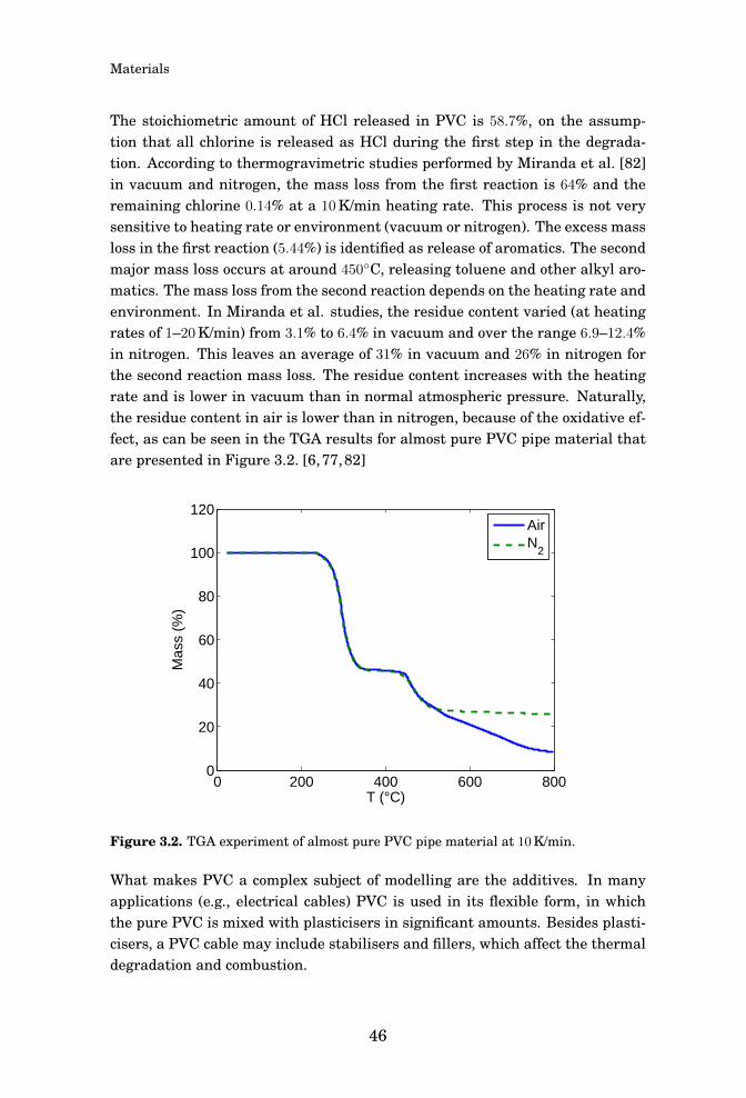
Materials

The stoichiometric amount of HCl released in PVC is 58.7%, on the assump-tion that all chlorine is released as HCl during the first step in the degrada-tion. According to thermogravimetric studies performed by Miranda et al. [82]in vacuum and nitrogen, the mass loss from the first reaction is 64% and theremaining chlorine 0.14% at a 10 K/min heating rate. This process is not verysensitive to heating rate or environment (vacuum or nitrogen). The excess massloss in the first reaction (5.44%) is identified as release of aromatics. The secondmajor mass loss occurs at around 450◦C, releasing toluene and other alkyl aro-matics. The mass loss from the second reaction depends on the heating rate andenvironment. In Miranda et al. studies, the residue content varied (at heatingrates of 1–20 K/min) from 3.1% to 6.4% in vacuum and over the range 6.9–12.4%in nitrogen. This leaves an average of 31% in vacuum and 26% in nitrogen forthe second reaction mass loss. The residue content increases with the heatingrate and is lower in vacuum than in normal atmospheric pressure. Naturally,the residue content in air is lower than in nitrogen, because of the oxidative ef-fect, as can be seen in the TGA results for almost pure PVC pipe material thatare presented in Figure 3.2. [6,77,82]

0 200 400 600 8000

20

40

60

80

100

120

T (°C)

Mas

s (%

)

AirN

2

Figure 3.2. TGA experiment of almost pure PVC pipe material at 10 K/min.

What makes PVC a complex subject of modelling are the additives. In manyapplications (e.g., electrical cables) PVC is used in its flexible form, in whichthe pure PVC is mixed with plasticisers in significant amounts. Besides plasti-cisers, a PVC cable may include stabilisers and fillers, which affect the thermaldegradation and combustion.

46

Materials

The most important additive from angle of the fire spread is the plasticiser,concentrations of which can be as high as 100 phr (parts per hundred partsresin). There are several commercial plasticisers available, of which one ofthe most commonly studied (and used) is diethylhexyl phthalate (DOP). Thephthalates degrade at around the temperature at which the dehydrochlorina-tion reaction occurs and releases combustible gases that burn with a flame inthe presence of oxygen. Besides increasing the fire risk through the mecha-nism of flammable gas, plasticisers interact with the PVC resin and alter thethermal degradation process. Marcilla and Beltran [81] studied pure samplesof DOP and PVC and their mixtures in TGA. The degradation temperaturesof these two components are slightly different; DOP degrades at slightly lowertemperatures than pure PVC. In a mixture, the temperatures almost overlap;the degradation temperature of DOP increases only slightly, but the PVC de-grades clearly earlier than it does without plasticisers. The low concentrationsof plasticiser and high heating rates decrease the effect. Similar destabilisationof the PVC was observed by Jimenez et al. [79]. They provided two explana-tions for the phenomenon: As the DOP evaporates, it leaves holes in the resinstructure that act as the starting points of the HCl release. Another cause maybe the reaction accelerating radicals formed at around 300◦C as the DOP evap-orates. Additionally, it was observed that DOP partially inhibits the formationof aromatics during the dehydrochlorination reaction.

The most significant additives in PVC mixtures, by concentration, are fillers.Reasons for the use of fillers range from improving the flame resistance (viaminerals ATH and MDH), thermal stability (via calcium carbonate, CaCO3),and electrical (via metal and carbon fibres) and mechanical (for example, viatalc) properties to simply cost reduction. In PVC cables, the most common filleris CaCO3. [88] It degrades at high temperatures, producing CO2 and H2O. Itmay also react with HCl to produce calsium chloride (CaCl). [89,90]

Other significant groups of additives are stabilisers and metal oxides. Theyare not added in large quantities but do have an effect on the thermal degra-dation of the polymer. Stabilisers do not directly affect the degradation temper-atures, but they do inhibit the formation of HCl, which is an important resultfrom the environmental point of view. At higher concentrations (> 1 phr), thesestabilisers also inhibit the benzene and toluene formation, thus decreasing theamount of combustible gases. [79] The metal oxides also suppress the formationof aromatics, for unsubstituted aromatics (benzene, and naphthalene), the ef-fect being more significant than for alkyl-aromatics (toluene). The oxides withthe greatest aromatic suppression effect also promote char formation the most.Some metal oxides (mainly ZnO) also lower the dehydrochlorination tempera-ture. [77]

47

Materials

3.5.2 Electrical cables

Fire is considered one of the initial events to be examined in PRA for nuclearpower plants. Electrical cables account for a significant portion of their fire load,and so cable fires have been widely studied both nationally [4] and internation-ally [91]. The fire itself is not the only hazard in those applications; also, failureof critical instrumentation or control cables may lead to severe consequences.

Early on cable modelling concentrated on simple, analytical models and ap-proximations [92,93]. With advances in processing power and CFD code, actualprediction of the fire spread, starting with the material reactions, has becomemore feasible. The dissertation project concentrated on the new methods formodelling cable fires more accurately.

As was noted earlier in this chapter, obtaining information about cable com-position may be challenging on account of lack of information. Some cables in anuclear power plant may have been installed decades ago and leave no way ofidentifying the cable composition except through extensive analysis of each ca-ble individually. It is fortuitous that knowing the exact compound does not seemto be as critical for the modelling as it is to be able to predict the effective be-haviour of the material. The small scale experiments (TGA, DSC, and possiblyMCC) in combination with a bench scale experiment (use of a cone calorimeter)provide enough information for building of an accurate model.

With cables, the geometry and structure pose the biggest challenges. Thecylindrical, non-uniform structure of a cable is impossible to model exactly viaCFD code, in consequence of the limitations of the grid and material definitions.It is important to understand that the model is not, and does not need to be, animitation of the reality in full; it is an approximation in which all the param-eters taken together compensate for the shortcomings and uncertainties of themodel (see Subsection 2.4.3).

Therefore, there are alternative ways to model a cylindrical, non-uniformobject. The simplest way is to project the cylindrical geometry to Cartesiancoordinates, modelling the cables as rectangular blocks. In this case, the largescale model is limited for the gas phase grid by the dimensions.

An alternative method, still under development, is to use sub-grid-scale(SGS) objects (in FDS, called Lagrangian particles) [43]. In SGS the particlesbehave equivalently to water droplets, but they may have surface propertiesof solid blocks. For particles, using a cylindrical form is feasible, and, there-fore, the geometry can be interpreted more accurately. The challenges with theparticles are related to radiation, flow drag and increased computation time.

The non-uniform layered structure is even more difficult to address. Sincemost cables do not have separate layers neatly ordered from the surface to core,

48

Materials

one has to approximate this too. Fortunately, other modelling parameters com-pensate also for this inaccuracy. The sheath layer is always on the exteriorboundaries, first and last layers in the Cartesian, only the first in the cylindri-cal. The rest of the layers can be combined in accordance with the modeller’spreferences. For example, the insulation and filler components may be takenin combination as a homogeneous layer, and the conductor may or may not beincluded in the model, since it does not degrade. An example of a cable modelin two geometries is shown in Figure 3.3. It could be argued, that the non-combustible metal conductor needs to be included, since it operates as a heatsink and therefore participates in the process of thermal degradation, but thiseffect can be modelled through suitable adjustment of the thermal parametersof the other layers. In many large scale calculations, pyrolysis calculations forthe solid obstacles are relatively time consuming, so it may be beneficial inthose cases to keep the model as simple and thin as possible. However, all thedegrading components should still be included, and with use of their actualmass fractions.

Figure 3.3. Examples of approximation of cable structure in Cartesian and cylindricalgeometries.

Often in the NPP applications, it is important to know whether or not the cablecan continue operating. Several models have been developed for calculatingthis [94,95]. It has been shown experimentally that most PVC cables fail whenthe temperature within the cable exceeds 200◦C. [94]

Since the cables lie in their cable tunnels for decades in varying conditions,it have to be considered that their properties may change. The important ques-tion is whether this increases the flammability of the cables. Some experimen-tal studies have been performed that compare new and old PVC cables, and

49

Materials

it seems that the time of ignition is actually longer with old cables. The ex-planation may have to do with slow evaporation of the phthalates, leaving lesscombustible material in the cable. [96,97] Another question is how the evapora-tion influence the cable’s mechanical properties. Placek and Kohout [98] studiedPVC-sheathed cables after exposing them to radiation and high temperatures,corresponding to 10 years of real-world service. They noticed that mechanicalproperties (strength and elongation) in the sheath area were not significantlyinferior to those of the new sample. However, in the insulation the effects weremore significant, especially with slow ageing. These effects were connected withoxygen diffusion causing extensive degradation. The model for calculating thetime of simulated ageing has been presented by Benes et al. [83].

3.5.3 Composites

Composites are made of two or more materials that are united through artificialcombinations. The artificial fabrication is an important feature differentiatingcomposites from, for example, metal alloys. Composites have the advantageof combining properties of two or more materials and therefore have qualitiesthat individual components cannot attain alone. They can be tailored in manyways through careful choice of the components and their proportions, the distri-butions, morphologies, degrees of crystallinity, crystallographic texture, struc-ture, and the composition of the interface between the components. Compositescombining suitable qualities in these categories can be lightweight, stiff, strong,resistant to corrosion, durable, and thermally isolating, and they can have lowthermal expansion, among other characteristics. [99,100]

The idea behind composites is not new. The first known composites weredeveloped by the ancient Egyptians when they reinforced their mud and claybricks with straw and developed the first version of plywood by combining manythin layers of wood into one thick layer [101]. Composites were used in the con-struction of the Great Wall of China (starting in 121 BC) too, where earth-workswere connected and reinforced with bricks that included, along with water andfine gravel, red willow reeds and twigs. In Mongolia, bows were made via lami-nation of animal horns and tendons, wood, or silk around 1200 AD [102]

Since those days, civil engineers and designers have striven to develop newforms of materials for stronger, larger, better, and more aesthetically pleas-ing structures. Since the 1960s, the use of polymer composites has grown veryrapidly. Composites are used in applications from aircraft and race cars tosporting goods and consumer products. [101, 103, 104] Biodegradable and lig-nocellulosic fibre composites have been developed since the 1990s, because ofthe growing interest in eco-friendly materials and increased prices of oil [102].

50

Materials

Some challenges with composites are related to their mechanical properties,low through-thickness, poor toleration of impact damage, and anisotropic prop-erties. One major disadvantage is their poor performance in fire. Some compos-ite matrixes soften, creep, and distort already at relatively low temperatures(> 100–200◦C), which can lead to problems with load-bearing installations. Or-ganic fibres used to reinforce the composite also decompose in higher temper-atures (300–400◦C), releasing fuel gases, which leads to fire in the presence ofoxygen. The consequences of this fire include heat, smoke, and toxic gases. Thefire products with combination with the decreasing structural durability makethe fire behaviour of this type of composites extremely dangerous. [100]

Composites are seeing increasing use in the aeronautical industry thanks totheir low density and their strength, along with the possibility they present foroptimising the design to achieve the best strength–weight and stiffness–weightratios. In aeroplanes, the high flammability of composites causes a huge risk,since evacuation possibilities are limited. In 1987–1996, only 3.5% of accidentson aeroplanes originated through fire. Although the number of the accidentswas small, they had the fourth largest contribution to the total casualties of allaccidents, causing 339 deaths over that nine-year period. Most accidents relatedto fire on the aeroplanes originate from outside from a fuel tank explosion. Inthose cases, the integrity and thermal resistance of the cabin are fundamentalfor the survival of the passengers. Composites display high thermal stabilityand slow conduction of heat through the thickness; therefore, they are moresuitable for use as thermal barriers than, e.g., metal alloys. The high flamma-bility of the composites can be improved by various mechanisms, including heatsinks, heat barriers and fillers that act in the solid or gas phase, in variousways. [2,7,100,105–107]

Research and modelling of the thermal behaviour of fibre-reinforced poly-mer composites had its beginnings in tandem with the defence and aerospaceindustries’ concentration on carbon fibre materials. The first person to modelmechanical properties at elevated temperatures was Springer, who did so in1984 [108]. He related the mechanical properties empirically to mass loss. Sincethen, the models have improved greatly, especially in terms of elastic and vis-coelastic behaviour at elevated or high temperatures. Bai and Keller [109] pro-vide a good overview of the thermomechanical models developed thus far.

The modelling of thermal degradation of flame retardant polymer compos-ites has been widely studied in the past few years. In 2000, Dembsey and Ja-coby [110] studied ignition models for marine cored composites and concludedthat the ignition models in use at the time were not able to predict the effectof skin thickness and core composition. A good compilation of analytical mod-els for composites in various circumstances has been presented by Lattimer

51

Materials

and Cambell [111]. A common trend in recent years has been to model thethermal degradation of the materials by using Arrhenius-type kinetics with thethree generally unknown parameters per reaction that are as discussed in Sec-tion 2.2. This approach has been successfully applied for composite materialsby Kim et al. [112] and by Lautenberger et al. [113]. Trelles and Lattimer [114]have suggested an alternative model that is based on the relationship betweendensity and temperature. That model shows good agreement with the experi-mental data.

52

4. Methods

4.1 Motivation

This chapter presents methods and applications developed during the work forthis dissertation. These methods have been applied and described in detailin the Publications I-V. First is discussion of the parameter estimation process,presenting the best practise and all of the experiences collected during the mod-elling work, from the sample preparation all the way to the model validation onlarge scale. The following sections present methods for the individual phasesof the modelling process. The FDS models for the experiments are briefly de-scribed, as are the parameter estimation methods used in this work. Finally,the method of combining TGA and MCC results is reviewed in brief.

4.2 The parameter estimation process

This section presents the best practise and observations gathered over the yearsof working with parameter estimation for various materials. A summary of theprocess is shown in Figure 4.1. It consists of four phases: sample preparation,experimental work, modelling and parameter estimation, and model validation.

The sample preparation is the preliminary phase to the experimental work.If the sample is not homogeneous and has several separable components, eachcomponent should be tested separately in the TGA. Therefore, the first step is todeconstruct the material. Some non-homogeneous materials cannot be decon-structed as easily, one example being fibre reinforced composites. In their case,it would be best to test the resin separately from the fibres. If the materialsare not available in pure form, small solid cubic forms will work better than apowder made of the sample. The decomposition energies change due to formingof powder, which lead to different results. Also, powder does not necessarilyhave the same component mass fraction as the original sample, so the resultsmay vary for that reason as well. When the components have been separated,densities and component mass fractions can be determined. At this point itis also necessary to study background information about the sample material.Relevant information would be what the typical additives are, what kinds ofreactions should be expected, and so on.

The experimental work includes all of the small and bench scale experi-ments. The TGA and DSC experiments are performed both in nitrogen andin air, ideally at several heating rates. The maximum temperature should be

53

Methods

set high enough that all the reactions end before the test is complete. A simi-lar principle holds for optional MCC results; if the reactions seem not to haveended when the test ends, or the oxygen content in the combustion chamberindicates that the material consumes all available oxygen, the test should berun again, with adjusted values. Cone calorimeter experiments should be doneat least at one heat flux, but results at other heat fluxes are very useful formodel validation purposes. Several, identical experiments should be conductedfor determination of the experimental error. The experiment should run untilthe flame extinguishes completely, not only to 20 minutes as the cone calorime-ter standard states. The useful measurements are the mass and heat releaserate, but in some cases also front and back temperatures of the sample are help-ful. An oxygen controlled cone calorimeter can be used for validating the solidphase degradation at the bench scale. The sample’s preparation is a complextask, especially for cables. Ideally, each component should be tested separatelyalso on cone calorimeter scale, but, except for the largest cables, the small sizeand the geometry of the cable components render this impossible. Therefore,cables are usually tested in cone calorimeter in whole form. The sample consistof several parallel 10 centimetre-long cables. The number of cables in a sam-ple depends on their diameter; each sample is approximately 10 cm wide. Theends of the cables should be wrapped carefully with aluminium foil to preventignition from the sides (insulation or filler).

Modelling and parameter estimation is the most important phase in thewhole process. It starts with determination of the reaction paths and kinet-ics for each component separately. The results of TGA and DSC are used fordetermining the number of reactions, and the results of MCC can be used inmeasurement of the reaction specific heats of combustion as explained in Sec-tion 4.5. The kinetic parameters are estimated from the TGA data. If the fitis acceptable, these values may be fixed in the subsequent steps. At this point,other measured properties (e.g., specific heat, reaction enthalpy, or heat of com-bustion) are fixed. These measurements are not mandatory, as the parameterscan be also estimated from the cone calorimeter results. However, the measure-ments decrease the possibility of the parameter compensation and help to keepthe model more realistic. The cone calorimeter model of any material can bemade in several ways, as explained in Subsection 4.3.2. For cables and com-posites, the layered structure and geometry may not be trivial to model. Whenthe model is chosen, the remaining parameters are estimated by fitting of themodel to the experiment. If the fit is not acceptable, it may be reasonable toreconsider the cone calorimeter modelling choices.

Model validation as the final step is an important but often neglected. In itssimplest form, it means comparing calculated and measured cone calorimeter

54

Methods

results at multiple heat fluxes that were are not used in the parameter esti-mation. The model should predict other heat fluxes at acceptable accuracy. Atlarger scale, validation is even rarer, since large scale experiments are not verycommonplace. This is a very important part of the associated software develop-ment.

1. Sample preparation

Deconstruct sample

Divide into components

Make measurements (e.g., density, mass fraction)

Study preliminary information about the sample material

TGA for each component

2. Experiments

3. Modelling and parameter estimation

4. Model validation

Cone calorimeter experiments

DSC (simultaneous or stand-alone)

MCC

Optional:

Determine the reaction path for each component separately

Estimate A, E, and N from TGA data

YesNo

Is the fit acceptable?

Fix A, E, N and measured values (Δα & ΔHc, cp, ΔH)

Cone calorimeter model

Estimate all of the missing parameters from cone calorimeter results

Validate the bench scale model, using other heat flux than for parameter estimation

No Yes

Is the fit acceptable?

Large-scale validation if possible

Figure 4.1. The material parameter estimation process.

4.3 FDS models of experimental methods

4.3.1 TGA and MCC

The TGA experiment is modelled for determination of the kinetics of the degra-dation reaction. The TGA model consists of a relatively large domain (4 m× 1 m× 1 m) and coarse grid (25 cm in the z-direction). The physical dimensions do notcorrespond to the real ones (the real sample cup has a volume of approximately40µl), but, since only the solid phase is being solved, the numerical solution ismuch more stable with larger dimensions than the actual sample size. Sinceonly the pyrolysis information is desired here, the gas phase calculations are

55

Methods

’turned off ’ by setting of the ambient oxygen level to be very low. The sample isvery thin (0.01 mm) and has a surface of 1 m × 1 m. The walls around the sam-ple are heated up linearly at the desired heating rate. During the heating, thesample mass and temperature are measured. The sample must be thermallythin enough to be in thermal equilibrium with the heating walls at all times.

An MCC experiment is modelled similar to a TGA experiment for thesepurposes, only with a higher heating rate (typically around 60 K/min). Sincethe pyrolysis takes place in inert ambient, only the solid phase is solved. Theheat release rate is the result of multiplying the mass loss rate by the heat ofcomplete combustion of the reaction species, which is defined by user.

4.3.2 Cone calorimeter

The cone calorimeter model used in this work consists of two parts: the coneheater and the sample. The sample is either a slab in the bottom of the compu-tational domain or at least one Lagrangian particle over an insulating board.The domain size is 0.3 m ×0.3 m ×0.4 m. The results are somewhat sensitive tothe grid size, but 5 or 10 cm has been found to be fast and accurate enough. Theresolution of the material model should, naturally, be based also on the finalapplication.

The model of the cone heater depends on the sample model. Traditionally,the heat flux is added directly to the slab-like surface. This is the easiest way be-cause the nominal heat flux of the cone heater at the surface can be determinedexactly as in the cone calorimeter. For more complex geometries, especially forthe Lagrangian particles, this approach does not work. In those cases, the up-per walls are set to high temperatures and thus direct a heat flux to the frontsurface of the sample. The temperature of the walls depends on the grid cellsize and other factors; hence, it should be measured for each set-up separately.

4.4 Estimation methods

The estimation methods discussed here have been developed for, and applied to,the estimation of the pyrolysis parameters. They were used extensively for theresearch presented in Publications I–V.

4.4.1 The generalized direct method

Various analytical methods used for obtaining the kinetic parameters of pyrol-ysis reactions were presented in Section 2.4. There are several, quite differentapproaches, some of them fast and easy to use and others providing very ac-curate estimates for prediction of the TGA curve. However, most of them are

56

Methods

somehow limited to special cases such as first-order reactions, one reaction step,or only non-noisy experimental data.

It is unfortunate that the real materials are often mixtures of several com-ponents; they may take part in multiple reactions, which cannot always be fullyseparated; and data can be noisy. Hence, a more general approach was devel-oped for Publication II and compared to other known methods.

For generalisation of the method for multiple reactions, a variable for thereaction progress is introduced,

α∗ =α− αk−1

αk − αk−1, (4.1)

where αk is the conversion after reaction k. The Arrhenius equation then be-comes for multiple reactions

dα

dT=Akβ

(αk − α)Nkαk − αk−1

exp

(− EkRT

). (4.2)

One reference point can be selected from the peak of the mass gradient. At thisreference point, the second derivative is 0 and the mass gradient at the peak is

rpk ≡ max(dα

dT

). (4.3)

The peak temperature and peak conversion, respectively, are Tp and αp, corre-spondingly. From the definition of the peak, the activation energy becomes

Ek = NkRrpk

αk − αpkT 2pk =

NkR

β

max(dα/dt)

αk − αpkT 2pk, (4.4)

depending on whether the derivative is calculated with respect to time or tem-perature. The pre-exponential factor can be calculated from eq. 4.2 with theactivation energy known:

Ak = rpkβ(αk − αk−1)Nk−1

αk − αpkexp

(EkRTpk

). (4.5)

This method, which is from here on called direct method (DM), is a fast andsimple way to define the pair (Ak, Ek), and reaction order can be calculated bymeans of some of the methods described in Subsection 2.4.1. For this method,only the location of the peak mass gradient and the total mass loss fraction ofthe reaction need to be known. However, if the reactions partly overlap in tem-perature (or time), determination of the peak may be challenging. Sometimesthere is also more noise at the highest mass loss rate, making the peak valuenon-exact. For this reason, the idea of the DM is developed further. If the refer-ence point could be selected more freely, e.g., before or after the peak, perhaps

57

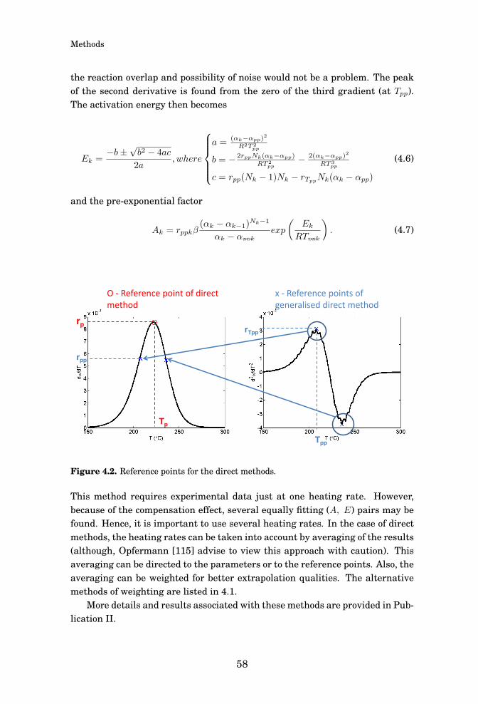
Methods

the reaction overlap and possibility of noise would not be a problem. The peakof the second derivative is found from the zero of the third gradient (at Tpp).The activation energy then becomes

Ek =−b±

√b2 − 4ac

2a,where

a =(αk−αpp)2

R2T 2pp

b = − 2rppNk(αk−αpp)RT 2

pp− 2(αk−αpp)2

RT 3pp

c = rpp(Nk − 1)Nk − rTppNk(αk − αpp)

(4.6)

and the pre-exponential factor

Ak = rppkβ(αk − αk−1)Nk−1

αk − αppkexp

(Ek

RTppk

). (4.7)

This method is known as generalized direct method (GDM). The reference pointsof both methods are illustrated in Figure 4.2.

O - Reference point of direct method

x - Reference points of generalised direct method

rp

Tp

rpp

rTpp

Tpp

Figure 4.2. Reference points for the direct methods.

This method requires experimental data just at one heating rate. However,because of the compensation effect, several equally fitting (A, E) pairs may befound. Hence, it is important to use several heating rates. In the case of directmethods, the heating rates can be taken into account by averaging of the results(although, Opfermann [115] advise to view this approach with caution). Thisaveraging can be directed to the parameters or to the reference points. Also, theaveraging can be weighted for better extrapolation qualities. The alternativemethods of weighting are listed in 4.1.

More details and results associated with these methods are provided in Pub-lication II.

58

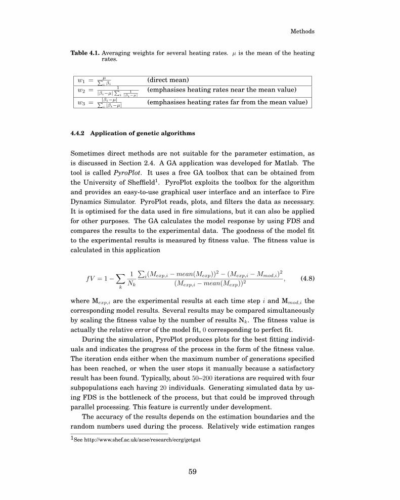
Methods

Table 4.1. Averaging weights for several heating rates. µ is the mean of the heatingrates.

w1 = µ∑i βi

(direct mean)w2 = 1

|βi−µ|∑i

1|βi−µ|

(emphasises heating rates near the mean value)

w3 = |βi−µ|∑i |βi−µ|

(emphasises heating rates far from the mean value)

4.4.2 Application of genetic algorithms

Sometimes direct methods are not suitable for the parameter estimation, asis discussed in Section 2.4. A GA application was developed for Matlab. Thetool is called PyroPlot. It uses a free GA toolbox that can be obtained fromthe University of Sheffield1. PyroPlot exploits the toolbox for the algorithmand provides an easy-to-use graphical user interface and an interface to FireDynamics Simulator. PyroPlot reads, plots, and filters the data as necessary.It is optimised for the data used in fire simulations, but it can also be appliedfor other purposes. The GA calculates the model response by using FDS andcompares the results to the experimental data. The goodness of the model fitto the experimental results is measured by fitness value. The fitness value iscalculated in this application

fV = 1−∑

k

1

Nk

∑i(Mexp,i −mean(Mexp))

2 − (Mexp,i −Mmod,i)2

(Mexp,i −mean(Mexp))2, (4.8)

where Mexp,i are the experimental results at each time step i and Mmod,i thecorresponding model results. Several results may be compared simultaneouslyby scaling the fitness value by the number of results Nk. The fitness value isactually the relative error of the model fit, 0 corresponding to perfect fit.

During the simulation, PyroPlot produces plots for the best fitting individ-uals and indicates the progress of the process in the form of the fitness value.The iteration ends either when the maximum number of generations specifiedhas been reached, or when the user stops it manually because a satisfactoryresult has been found. Typically, about 50–200 iterations are required with foursubpopulations each having 20 individuals. Generating simulated data by us-ing FDS is the bottleneck of the process, but that could be improved throughparallel processing. This feature is currently under development.

The accuracy of the results depends on the estimation boundaries and therandom numbers used during the process. Relatively wide estimation ranges

1See http://www.shef.ac.uk/acse/research/ecrg/getgat

59

Methods

are recommended, for yielding the best possible solution, unless the variablevalue is known approximately. Because of the stochastic nature of the algo-rithm, the results are slightly different every time. Especially if there are sev-eral solutions, with equal fit (as is typical among TGA results), the solution mayconverge to very different numbers each time. On occasion an overall fit cannotbe found. This may be the case with the cone calorimeter results because of thegeometry and layer approximations. In those cases, it is convenient to choosecertain parts of the curve (e.g., ignition time and/or the location of the first peak)that have more weight in the fitness value than the other points. This helps thealgorithm converge to more acceptable solutions.

PyroPlot can be obtained from Google Code2 under the MIT License. Moreinformation about genetic algorithm and it’s application to fire parameter esti-mation is reported in Publication I.

4.4.3 Sensitivity analysis

Despite of the method used to estimate the model parameters (thermal or ki-netic), sometimes there is a need to adjust them manually for obtaining a betterfit with the experimental results. In order to do that effectively, understandingof the correlations between model input and the results is required. A sensitiv-ity study was performed for a generic, charring material in the cone calorimeterat 50 kW/m2 by changing one model parameter at a time. From the results ofthis sensitivity study, rules of thumb were formulated for summarising the re-sults. These rules are listed in Table 4.2. Definitions for the results are shownin Figure 4.3.

The parameter values were chosen such that the two peaks were well de-fined. That is not always the case, if the second peak occurs very soon afterthe first one. The first peak of the two-peaked shape of a charring materialcomes from the protective char layer building up as a result of the pyrolysis.It increases the thermal resistance between the exposed surface and pyrolysisfront, which leads to a decrease in the heat release rate after the maximumis reached. In the cone calorimeter, the back of the sample is often insulated,which prevents heat losses from the back side. Therefore in the end, when thepyrolysis front reaches the back, the heat release rate increases to the secondpeak. The two peaks overlap in time if the thermal conductivity is high for boththe virgin material and residue.

The single most important parameter for all the results turned out to bethe activation energy, or the pair (A, E). The emissivities of both virgin andresidue components were also significant in almost all cases. For the ignition

2http://code.google.com/p/pyroplot/

60

Methods

time, the other important parameters are thermal conductivity, specific heat,and the absorption coefficient of the virgin material. The time of the first peakis additionally affected by the heat of combustion (in the cases with ambientair). The first peak’s height depends also on the heat of reaction of the virginmaterial, and on the properties of the residue. The time of the second peakand its height depend on all the parameters except the reaction order of thevirgin material, and the specific heat of the residue. For flame-out time, all theparameters are significant, apart from the specific heat of the residue.

A similar study has been performed by Stoliarov et al. [116]. They conductedan extensive literature review of the values for several polymers and simulatedthe model at minimum, maximum, and mean values under several radiant heatfluxes and initial thicknesses. The pyrolysis was modelled by means of thecalled ThermaKin software, mentioned above. It has a slightly different py-rolysis model than FDS uses. The charring process was not included in themodel, but char yield was taken into account. Stoliarov and colleagues stud-ied the variation effects on mass loss rate (MLR), instead of heat release rate.They considered four results: time to mass loss (corresponding to tig), time topeak MLR (t1st_p), peak MLR (comparable to Q1st_p), and average MLR (notpresented in Table 4.2). The results were similar, in view of the differences inthe models. For time to ignition, the most important parameter is the ratioA/E. This makes sense, because increasing E and/or decreasing A moves thereaction to higher temperatures. In fact, this ratio turned out to be the most im-portant parameter of all the results studied. Thermal conductivity and specificheat capacity both increase the ignition time, and heat of reaction was found tohave no significant effect, in both studies. The differences are in the absorptioncoefficient and reflectivity (defined as 1 − ε); where the effect is opposite thatpredicted in the study with FDS (see Table 4.2). For the time of peak, all ofthe other results are similar except those for the thermal conductivity (positivecorrelation with FDS and negative in the study of Stoliarov et al.) and reflectiv-ity. The results for the peak height are similar between the two studies (exceptagain for the reflectivity). The differences may be due to the differences in themodel, mainly inclusion of the charring reaction in the model.

4.5 MCC methods

Two methods for combining TGA and MCC results have been developed. Thefirst one discussed here is simple and easy to use, while the second is aimedat explaining the material composition more accurately. These methods arepresented also in Publication IV.

61

Methods

Table 4.2. Rules of thumb for charring material, where + means a slight increasing,++ substantial increasing, - slight decreasing and - - substantial decreasingeffect in the result, when the particular parameter is increased.

tig t1st_p Q1st_p t2nd_p Q2nd_p tflameoutVirgin materialA - - - - + + -E ++ ++ - - ++ - ++N +k + + - - + -cp + + - ++ - +∆H - + - - ++∆Hc + ++ - ++ -κ + + + - +ε ++ ++ - - ++ - ++Residuek + ++ - -cp -ε ++ - + - -

t1st_peak,Q1st_peak

t2nd_peak,Q2nd_peak

Time of ignition

Time of flame out

Figure 4.3. Definitions for the rules of thumb.

4.5.1 Method 1

Method 1 could be called an engineering tool. It does not require any infor-mation about the material or its composition; it is merely a way of efficientlymodelling the correct amount of heat for each reaction. No special softwareis needed either. A simple reaction path is assumed: Each reaction step cor-

62

Methods

Table 4.3. Input parameters used in generation of the table of rules of thumb.

Parameter (unit) Baseline New valueA (s−1) 1·1018 → 1·1017

E (J/mol) 2.5·105 → 2.0·105

N 2 → 1k (virgin and residue) (W/m·K) 0.8 → 0.4cp (virgin) (kJ/kg·K) 2.5 → 1.8cp (residue) (kJ/kg·K) 2.5 → 1.5∆H (kJ/kg) 800 → 400∆Hc (MJ/kg) 40 → 20κ (1/m) 50000 → 500ε 1 → 0.5

responds to one pseudo-component in the model. Each pseudo-component canyield one fuel and one inert gas. The heat of combustion (∆Hc) is fixed for all ofthe reactions. Only the last reaction may yield residue.

The fuel yield (yi,F ) of each reaction (for all i < nr) can be calculated from

yi,F =Qi/m0

∆Hc∆αi, (4.9)

where Qi/m0 is the MCC result (heat of complete combustion scaled by initialmass of the sample) and ∆αi the relative mass loss of reaction i as observed inTGA. The inert gas yield is thus yi,I = 1− yi,F .

If the material does not yield residue, eq. 4.9 can be used also for the lastreaction. If the material does produce residue, the yields of the last reactionbecome

ynr,F =Qnr/m0

∆Hc∆αnr(1− Z

1−∑nr−1i=1 ∆αi

)

ynr,I = (1− Qnr/m0

∆Hc∆αnr)(1− Z

1−∑nr−1i=1 ∆αi

),

ynr,Z = 1− ynr,F − ynr,I = Z

1−∑nr−1i=1 ∆αi

(4.10)

where Z is the residue yield of the original mass.

4.5.2 Method 2

Method 2 is intended for the more ambitious modeller who wants to estimatethe reaction path and material composition more accurately. The reaction pathcan be chosen freely, including several parallel, consecutive and even competi-tive reactions, each yielding several gases and residue. As the reaction path isfixed and can be very complex, there is no analytical way to solve this. There-

63

Methods

fore, the case is constructed as an optimisation problem wherein the objectivefunction is to minimise error between the measured and estimated values. Thevariables are the initial mass fractions of the components, gas yields and theheat of combustion of each gas. One can include inert gas by setting the heatof combustion to 0. The estimates for the mass loss and energy release of eachreaction are

∆αi =∑ncj=1

∑np,jk=1 yi,j,kYi−1,j

Qi =∑ncj=1

∑np,jk=1 yi,j,kYi−1,j∆Hc,k,

(4.11)

where Yi, j is the mass fraction of component i after reaction j. The calculationis performed recursively from the previous reaction steps;

Yi,j =i∏

ii=1

yii,j,ZYi−1,j . (4.12)

The estimation can be performed with using any non-linear solver software,such as, Excel Solver or Matlab Optimization Toolbox. Since the result dependssignificantly on the initial values, the optimisation is performed through repe-tition of the process several times with random initial values from the selectedrange. In this application, the optimisation was made by means of a Matlabfunction.

4.6 Estimation of the uncertainties

4.6.1 Experimental error

On small scale, the greatest experimental error is related to the sample prepa-ration. The experiments are, in general, highly repeatable if the conditions andthe sample are kept identical. This can be seen in Figure 4.4, where the resultsof repeated MCC experiments are shown for samples of birch wood. The sam-ples were taken from the same board, and some of the board was dried in anoven at 105◦C over a weekend for removal of all moisture. The total heat releaseof the non-dried wood varies with in the range 11.1–11.2 MJ/kg, with the max-imum heat release rate being 164–178 kW/kg and the temperature at the peakbetween 374 and 376◦C. The heat release rate the dried wood is higher, becausethe original mass is purely combustible wood. If the results for non-dried woodare scaled in view of the mass of the water (6%), the results look very similar.The difference between the dried material and scaled results is 2.9% for thetotal heat release, 3% for the peak heat release rate and 0.2% for peak temper-ature. Although the dried sample is kept in a desiccator, it is quite unclear how

64

Methods

much moisture the dry sample absorbs during the preparations (measurement,sample positioning and heating of the furnace). Therefore, it may be more con-venient to test the sample as delivered and determine the moisture content byusing another sample.

200 300 400 5000

50

100

150

200

T (°C)

HR

R (m

W/m

g)

Exp 1Exp 2Exp 3

200 300 400 5000

50

100

150

200

HR

R (m

W/m

g)

T (°C)

Moist. 6 %Moist. 6 %, scaledDry sample

a b

Figure 4.4. Repeated MCC experiments with birch wood. a) non-dried wood, moisture6% and b) non-dried and dry wood.

The sample mass should be small enough for keeping the sample in thermalequilibrium with the furnace at all times. This is dependent on the thermalthickness of the sample and the heating rate. Also the load cell accuracy issignificant with the smallest samples. If the accuracy is 0.1 mg, 10% error couldresult for the smallest samples.

In the cases involving non-homogenous materials (such as composites), thesample preparation is especially challenging. The material may be very hard tocut, one may be tempted to grate it into powder. In the approach described here,the problem may lie in preserving the sample mass fractions. For example, longfibres may be too big for the sample cup and therefore omitted, leading to lowerfibre content and thus greater content of combustibles.

4.6.2 Uncertainties in the modelling

The material model’s uncertainty on the larger scale depends on the accuracy ofsaid model and the modelling software. The accuracy of FDS can be evaluatedvia the verification and validation guides [117,118]. The verification guide con-sists of simple examples to verify that the code is implemented correctly, andthe validation guide includes a comparison of the experiments and models toconfirm that the physics of the several phenomena involved have been handledaccurately.

Material model accuracy one the large scale depends on the accuracy of

65

Methods

the small and bench scale model. As is proved in Publication III, it is not theparameter values that are significant on bench scale but the overall fit. Thevalidation work on large scale will continue.

66

5. Results

5.1 Motivation

This chapter includes summary of the most important results described in Pub-lications I-V and some additional results that shed light on and explain thework done for this dissertation. The estimation methods presented in Publi-cation I and Publication II are compared to other methods in use in terms ofaccuracy, effectiveness, and ease of use (in Section 5.2). The main results of thesensitivity study performed for Publication III are listed in Section 5.3. Somenew results of testing of a PVC cable with the MCC methods developed in thework on Publication IV are reported in Section 5.4, and, a sensitivity study ofthe cable model used in the large scale MC simulations covered in PublicationV is presented in Section 5.5.

5.2 Comparison of estimation methods

The range of estimation methods suitable for extraction of the parameters forpyrolysis models is wide, and often the choice is based on the personal pref-erences of the modeller. The methods can be divided roughly into two groups,as discussed in Section 2.4: analytical and curve-fitting algorithms. The lattercan be applied to any model (including the estimation of thermal parameters),but the analytical methods are model specific. Publication II summarises somecommonly used methods for the estimation of kinetic parameters and comparestheir results’ accuracy, their efficiency, and the complexity. The set of meth-ods included two evolutionary algorithms (a GA and SCE) and four analyticalmethods, of which one was derived by the author and the others were foundin the literature [40, 42, 43]. These methods were tested against two sets ofgeneric experimental data. Generic data were chosen because of the possibilityof comparing the real target values to the estimated ones. The first data set wasvery simple and noiseless, and the reactions were well separated in time. Thesecond data set was more complicated including noise and partly overlappingreactions. Only the analytical methods were tested for data set 2. The inter-polation ability of the methods was tested at a heating rate that was withinthe range of experimental heating rates (20 K/min). The extrapolation abilitywas tested at a significantly higher rate, 100 K/min. The parameters were alsoevaluated on larger scale, with the cone calorimeter model and fixed thermalparameters.

67

Results

The results are summarised in Table 5.1. The reference values were cal-culated from the generic data. For accuracy of the results, when one considersboth fitness values (as in eq.4.8) and difference in the target values, the evo-lutionary algorithms were superior to the analytical methods. For the former,the user has to define the variable ranges and algorithm parameters. If thealgorithm is used with default settings, six lower and upper boundaries haveto be determined. For analytical methods, the number of parameters (the com-plexity) did not correlate directly with the greater accuracy of results. However,the simplest method, the first-order McGrattan-Lyon [42,43] method, producedthe worst fit. The other analytical methods performed well, with good fit in thesolutions for both data sets and also for noisy data.

As for their level of accuracy for the end application, all methods testedproduce acceptable results. Hence, one can state that the choice of method isbasically up to the user.

Table 5.1. Comparison of the estimation methods based on two example cases. Fit-ness value is the relative error, 0 corresponding to perfect fit. 1With noise2. 2Without parallel computing (algorithms) or automated search for refer-ence values. 3For algorithms, estimation boundaries etc.

GA SCE DM GDM Friedman McGrattan-Lyon

Fitness value 0.0041 0.0003 0.0111 0.0082 0.0109 0.0131w/ data set 1

(at 100 K/min)Fitness value - - 0.0143 0.0181 0.0093 0.0553w/ data set 21

(at 100 K/min)Time of 10 min 10 min 0 min 0 min 0 min 0 min

preparationTime of ≈ 1 day ≈ 1 day 10 min 15 min 15 min 5 min

estimation2

Number of min. 12 min. 12 10 12 16 8reference values3

5.3 Sensitivity and uncertainty of the model

For Publication III, various modelling choices were tested in modelling of a PVCcable sheath material. The versions tested included the following:

• Reaction scheme (parallel or consecutive)• Char formation (which reaction produces char)• Values of the kinetic parameters ((A,E) pairs)• The value of the reaction order• The fuel yield of the first reaction.

68

Results

The reaction scheme can typically be either parallel (components degradeindependently of each other) or consecutive (one component degrades to an-other). In some cases, also competing reactions may be relevant. For example,for cellulose degradation, different reaction paths are known to dominate, de-pending on the temperature and heating rate. At low temperatures, the domi-nant process is intermolecular dehydration leading to char and gas, and in thepresence of air to smouldering combustion. At high temperatures, depolymeri-sation predominates in the process and leads to tar and flaming combustion inair [119]. All three general reaction paths are presented in Figure 5.1. Thecombinations of them are possible also.

Parallel: Consecutive: Competing:

A → B A → B → C BC → D A

C

Figure 5.1. Possible reaction paths in pyrolysis modelling.

The reaction path significantly affects the kinetic parameters values, whichsupports the interpretation that the parameters are model-dependent ratherthan material properties. Equally good fits can be achieved with any reactionpath, but the parameters and the reaction paths cannot be used separately.This difference is clearer with the cone calorimeter results. The consecutive re-action path results in significantly slower degradation when the same thermalparameters are used. This happens because the next reaction is always limitedby the previous one in the consecutive reaction path, and at high heating ratesand with fixed thermal parameters the reactions overlap more in the parallelpath than is possible with the consecutive path. With fitting of the thermalparameters for each reaction path, equally good fit is again reached.

Another modeller decision is that on distribution of char forming. When aparallel reaction path is used, the char can be formed from any reaction(s). Onsmall scale, this does not make any difference, and with the version of FDS (ver-sion 5) used for the simulations reported upon in Publication III it did not makeany difference on cone calorimeter scale either when the char conductivity washigh enough. Version 6 of FDS includes a new ability for modelling swellingsurfaces. Char is known to swell and form an insulating layer at the material’ssurface. The amount of swelling depends on the density of the residue compo-nent, and, therefore, it does make a difference at which reaction char is former,

69

Results

and in what quantities (as seen earlier, in Figure 3.1).As mentioned above, the values of A and E are unambiguous because of

the compensation effect [60], so several pairs that fit equally well can be found.Two sets of parameters (N being 1) were estimated by means of GA and ananalytical approach. The results showed that if the reaction path and order arethe same, and the kinetic parameters fit equally well on small scale, they causeno difference on the larger scale either. Naturally, small differences in the fit atsmall scale may lead to larger differences on the larger scale. In addition, thisstudy confirmed that the results are not sensitive to the estimation method, asdiscussed in Section 5.2, above.

The reaction order is the parameter that compensates for the inaccuracy inmodelling of the chemical reactions. In other words, it is the parameter thatlumps several reactions together and defines the sharpness of the TGA curve.The results show that this is an important parameter: two sets of parametersthat on small scale had equally good fit, resulted in very different heat releaseand mass loss rate curves in the cone calorimeter context with the same thermalparameters. The lower reaction rate led to slower degradation of the samplematerial.

Although pure PVC releases only a small quantity of combustible gases dur-ing the first reaction, this is often not the case for the real PVC cable material.These materials contain large amounts of additives, including plasticisers thatdegrade at around the same temperatures as pure PVC (dehydrochlorinationreaction), releasing highly flammable gases. This should be taken into accountwhen one builds a PVC model, even if it is not detectable in the TGA results.Alternative methods for defining the fuel yield are presented in Section 4.5, buta fast way to estimate the fuel content of the sample is fitting to the heat releaserate curve of the cone calorimeter results. Also making a big difference for theresults is whether one allows fuel gas release from the first reaction too.

Summarising the results, one can state that most of the modeller choicesdo not have any significant effect on the bench scale experimental results butthey do have an effect on the parameter values used. This means that the pa-rameters really are model-dependent and should not be considered independentmaterial characteristics, and it means in consequence that these values shouldnot be mixed or used outside the intended application.

5.4 Estimation of the cable composition via MCC

The MCC methods were applied to a PVC sheath of an electric cable (#701)for Publication IV. Now method 2 has been used for estimating the reactionpath for another cable, identified as MCMK, which was also used in the sensi-

70

Results

tivity study of Publication III. The TGA experiments were performed at heatingrates of 2, 10, and 20 K/min, and the MCC analysis was repeated three timeswith a pyrolysis temperature of 75 to 900◦C, 900◦C combustion temperature,and 20 cm3/min flow of oxygen to the combustor. In TGA, three clear peaks canbe observed and in MCC two. An additional, very weak peak may be observednear the end of the MCC experiment at around 700◦C, but it is so weak that itcan be ignored. The averages of the experimental results are listed in Table 5.2.

Table 5.2. Experimental MCC results for the MCMK sheath (the values are averagesover three repetitions and heating rates).

Reaction 1 Reaction 2 Reaction 3 TotalTp (◦C) 282 462 728 -∆α in TGA 0.56 0.10 0.07 0.74∆α in MCC - - - 0.74Q/m0 (MJ/kg) in MCC 10.5 4.2 0 14.7

The iterative estimation process explained in Section 4.5 was repeated 5, 000

times, and the accuracy (or fit) of the final result is 1.5 · 10−7. The results arelisted in Table 5.3, where they are compared with the estimation results forcable #701. The mass fractions in the original material are denoted by Yi,and the fuel and inert gas yields with yF,ij and yI,ij , respectively. Index i isthe component index and j the reaction index. The results are quite different:They showed that according to assumptions on the reaction paths, the MCMKto consist of 29% PVC (i = 1), 39% plasticiser (i = 2) and 32% CaCO3 (i =

3), while the corresponding mass fractions for cable #701 are 51% , 27% and22%, respectively. The experimental results for both cable sheaths are shownin Figure 5.2. From the figures it can be observed that MCMK sheath has lessmass loss and higher heat release during the first reaction. This explains theresult of the higher mass fraction of plasticiser. The second-reaction mass loss ishigher for the #701 sheath, but the heat released during the reactions is almostthe same. Hence, the heat of combustion of the PVC residual must be higher.The third mass loss is higher for the MCMK; therefore, the amount of CaCO3

is probably higher in the MCMK. It should be kept in mind that while method2 allows more truthful reaction paths, the real accuracy always depends on theassumptions made by modeller. The cable sheath compositions presented heremay or may not correspond to the real composition, but the resulting modelis able to predict correct mass loss and heat release rate using more complexreaction path, as intended.

71

Results

Table 5.3. Estimation results for MCMK cable sheath compared with the results forcable #701 sheath.

Estimation Initial Result Resultboundaries values (MCMK) (#701)

Y1 [0.2,0.7] 0.26 0.29 0.51Y2 [0.1,0.5] 0.38 0.39 0.27Y3 - 0.35 0.32 0.22yI11 [0.57,0.61] 0.60 0.58 0.60yF11 [0,0.07] 0.00 0.00 0.04yF12 [0.5,0.9] 0.85 0.81 0.75yI33 [0.05,0.3] 0.21 0.22 0.18∆Hc,11 [25,50] 49.40 32.54 49.10∆Hc,12 [25,50] 30.38 42.00 35.80∆Hc,21 [25,50] 30.62 26.90 30.20

0 200 400 600 80020

40

60

80

100

T (°C)

Mas

s (%

)

MCMK 10 K/min#701 10 K/min

200 400 600 8000

50

100

150

200

250

300

T (°C)

HR

R (

mW

/mg)

MCMK (averaged results)#701 (averaged results)

a b

Figure 5.2. Comparison of experimental results for two PVC sheaths. a) TGA at10 K/min, and b) MCC at 60 K/min.

5.5 Application to a cable tunnel

Publication V applied the parameter estimation results to large scale simula-tion at a cable tunnel fire of a nuclear power plant. The diversity of the cablesfound at a real nuclear power plant was taken into account through variation ofsome of the cable model parameters in the MC simulations. A sensitivity studyfor the parameter values in cone calorimeter results is presented here.

A cable model used in Publication V was studied via MC technique withthe same parameter ranges as in the paper. The sample was generated bymeans of Latin hypercubes, and the sample size was 100. The variables were thethermal conductivity of the charring pseudocomponents of the sheath (sheath 1and sheath 2) and the thicknesses of the first three layers (sheath, insulation

72

Results

plus filler, and sheath). All distributions were assumed to be uniform sincethe idea was only to study the correlations between input and output. Fouroutput quantities were defined: time to ignition (defined as the time until HRR> 10 kW/m2 the first time), maximum heat release rate, time of maximum heatrelease rate, and time of flame out (the time until HRR < 10 kW/m2 in the endof the experiment). The correlations are shown as a scatter plot in Figure 5.3and as correlation coefficients in Figure 5.4. It can be seen that the thermalconductivity has the greatest correlation with all of the output quantities, andthe strongest correlation is with the time of ignition, as expected. The layerthicknesses correlated most strongly with the maximum heat release rate, andthe second layer’s thickness correlates also with the time of the maximum heatrelease rate. There is a little uncertainty related to definition of the maximumheat release rate, because of noise in the simulated data. For the flame-outtime, the only significant parameter was thermal conductivity.

0 0.1 0.2

40

60

80

100tig

(s)

0 0.1 0.2

100

150

200Max hrr (kW/m2)

0 0.1 0.2500

1000

1500

2000

2500

Thermal conductivity (W/m⋅K)

t (max hrr) (s)

0 0.1 0.21000

2000

3000

4000t (flame out) (s)

Figure 5.3. Output quantities versus thermal conductivity.

73

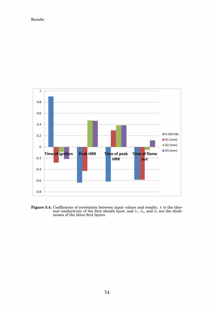
Results

-0.8

-0.6

-0.4

-0.2

0

0.2

0.4

0.6

0.8

1

Time of ignition Peak HRR Time of peak HRR

Time of flame out

k (W/mK)δ1 (mm)δ2 (mm)δ3 (mm)

Figure 5.4. Coefficients of correlation between input values and results. k is the ther-mal conductivity of the first sheath layer, and δ1, δ2, and δ3 are the thick-nesses of the three first layers.

74

6. Conclusions and future work

6.1 Conclusions and discussion

Since fires cause significant harm to people and property, being able to recognisethe risks is essential if one is to limit the consequences. For prediction of the firespread, it is necessary to model the pyrolysis of the solid phase, starting withthe chemical degradation reactions. This dissertation has focused on studyingthe methods of pyrolysis modelling, including the estimation methods, and bestpractises throughout the modelling process. The methods have been applied toone real-world-scale application in simulation of a cable tunnel fire at a nuclearpower plant.

Publication I and Publication II present methods for estimation of the pyrol-ysis model parameters. The semi-analytical models are simple and fast to use,and they are able to find estimates for the kinetic parameters that show accu-rate enough fit to the experimental data. Some of them even work for slightlyoverlapping or noisy data. An additional benefit with these methods is that theresult does not depend on the estimation process or on boundary values; the re-sult is always the same. However, for more complicated reaction paths or noisydata, the estimation algorithms offer a more robust method. Those algorithmsdemand more time and resources but are almost certainly able to find an accu-rate fit for the experimental data. They can also be used for the estimation ofother parameters besides kinetics. The main drawback and criticism of the py-rolysis modelling is that the kinetic parameters are rendered ambiguous by thecompensation effect. Depending on the stochastic nature of the algorithm andestimation boundaries, the algorithm may end up reaching a different solutionevery time. However, the work done in this dissertation project and the discus-sion above indicate that the bench and large scale results are not sensitive tothe kinetic parameters themselves, just relevant for the fit to the experimentaldata.

Publication III covers the modelling of a PVC material. Several modellingchoices are studied there and compared on bench scale. It turned out that themodel is sensitive to many choices (e.g., reaction path or order) when the samethermal parameters are used. However, results with equally good fit may befound for all the alternatives if the thermal parameters are fitted separately.This confirms that the parameters are model-specific and not material-specific.It is important that one does not take the parameters out of context and usethem in a different model, since they do not mean anything on their own. This

75

Conclusions and future work

study proved again that any particular estimation method is not significant forfinding the fit on the larger scale. As long as the reaction path and order arethe same and the result shows equally good fit on the small scale, the differencein order of magnitude does not matter with the pair (A,E).

The methods combining the results of TGA and MCC were presented in Pub-lication IV. These two methods were developed for different modelling needs:method 1 is very simple and can be used only for calculating the correct amountof heat from each reaction. The second method is more complex, and has theambitious goal of modelling the reaction path as accurately as is reasonable. Itcan also be used for estimating the composition of an unknown material.

The methods presented in the dissertation were tested in a real world sce-nario for a nuclear power plant (see Publication V). The cable trays were mod-elled by means of the genetic algorithm and small and bench scale data. Themodel was used as a basis for Monte Carlo simulations. The results providedvaluable information about the failure probabilities of the cables and the mostsignificant variables behind the most severe conditions. More specifically, thisstudy was used as a part of PRA for an actual nuclear power plant in Fin-land [4].

The methods and applications developed in this dissertation project have areal impact on the fire safety of the materials and public buildings in use. Ca-pability of accurately modelling and predicting the flame spread with differentfire loads improves the evaluation and identification of the risks and makes theallocation of resources more effective. The cable simulations have already con-tributed to the calculation of more realistic probabilities of fire spread, in theupdating of the PRA for the Finnish nuclear power plant. [120]

6.2 Future work and trends in pyrolysis modelling

Work to validate the current fire spread models continues on the large scale.The SGS modelling is expected to solve the current problems found in the CFDmodelling of the cables. Being able to model composite structures accuratelycould save significant amount of effort and expenses in real scale testing in thedevelopment phase.

The OECD project PRISME 21 will provide excellent large scale experimen-tal results for fires affecting multiple cable trays and electrical cabinets. Thetests are performed for various room configurations, and several measurementsare made in the course of any given test. The resulting data will be used for val-idating the entire process of pyrolysis modelling and parameter estimation asdescribed in Section 4.2, from the solid phase thermal degradation reactions

1see http://www.oecd-nea.org/jointproj/prisme-2.html

76

Conclusions and future work

through prediction of fire spread in large installations.Being able to model the thermal degradation reactions of a material accu-

rately opens new opportunities also in the area of material development anddesign. Modelling the flame retardancy mechanisms may be especially valu-able for the design of new, flame retardant materials. Correctly predicting thecooling effect of an endothermic reaction or the insulating effect of an insulatingchar barrier enables large scale testing via simulations before the material iseven produced. The concentrations of the additives can be studied numericallyfirst, which should decrease the effort of experimental trial and error.

Applications of the presented methods can also be found outside the firesafety engineering. For example, they could be used in developing new methodsfor extracting biofuels from the biomass as well. Understanding the thermaldegradation process of the biomass provides new possibilities for testing thealternative methods by modelling instead of performing experiments. [121–123]

An even smaller scale tool for studying the thermal degradation of mate-rials is molecular dynamics [13]. It calculates the behaviour of the moleculesnumerically, on the basis of knowledge of the interactions (forces) between themolecules. It allows study on such time and dimension scales as could not beaddressed otherwise. The tools of MD could indeed be used in studies of flameretardants. Studying additives’ effect in the resin at molecular level may signif-icantly aid in understanding the operation of the current flame retardants andin developing new and better ones.

77

Bibliography

[1] E. Kokki. Palokuolemat ja ihmisen pelastamiset tulipaloissa 2007–2010.Pelastusopisto, tutkimusraportti, 3, 2011.

[2] I. Lopez de Santiago, I. Saez de Ocariz Granja, A. Arbildi Fernandez,F. Fernandez Sanchez, A. Cortes Rueda, and K. Fernandez Horcajo. Firepenetration in an aircraft made in composite. Proceedings of the Interena-tional Congress on Combustion and Fire Dynamics in Santander, 2010.

[3] T. Hakkarainen, J. Hietaniemi, S. Hostikka, T. Karhula, T. Kling,J. Mangs, E. Mikkola, and T. Oksanen. Survivability for ships in case offire. final report of surship-fire project. VTT Research Notes 2497, 2009.

[4] E.-K. Puska and V. Suolanen. Safir 2010. the finnish research programmeon nuclear power plant safety 2007-2010. VTT Research Notes 2571,2011.

[5] S.V. Hoa. Principles of the Manufactoring of Composite Materials.DEStech Publications, Inc., 2009.

[6] E.S. Papazoglou. Chapter 4. flame retardants for plastics. In C.A. Harper,editor, Handbook of Building Materials for Fire Protection, pages 4.1–4.88. McGraw-Hill, New York, 2004.

[7] P. Hornsby. Chapter 7. fire retardant fillers. In C.A. Wilkie and A.B.Morgan, editors, Fire Retardancy of Polymeric Materials, Second Edition,page 163–185. CRC PressINC, 2009.

[8] Y. Zhang, Y.C. Wang, C.G. Bailey, and A.P. Taylor. Global modelling offire protection performance of intumescent coating under different conecalorimeter heating conditions. Fire Safety Journal, 50(0):51–62, 2012.

[9] A. Paajanen, T. Korhonen, M. Sippola, S. Hostikka, M. Malendowski, andR. Gutkin. Fds2fem - a tool for coupling fire and structural analyses.Proceedings of CMM-2013 - Computer Methods in Mechanics, Poznan,Poland, 2013.

[10] J. Vaari, S. Hostikka, T. Sikanen, and A. Paajanen. Numerical simula-tions on the performance of waterbased fire suppression systems. VTTTECHNOLOGY 54, 2012.

[11] T. Korhonen, S. Hostikka, S. Heliövaara, and H. Ehtamo. Fds+evac:An agent based fire evacuation model. In W.W.F. Klingsch, C. Rogsch,A. Schadschneider, and M. Schreckenberg, editors, Pedestrian and Evac-uation Dynamics 2008, pages 109–120. Springer Berlin Heidelberg, 2010.

[12] S. Hostikka, T. Kling, and A. Paajanen. Simulation of fire behaviour andhuman operations using a new stochastic operation time model. PSAM-11 -ESREL 2012 Conference. 25-29 June. Helsinki, 2012.

78

[13] K.D. Smith, M. Bruns, S.I. Stoliarov, M.R. Nyden, O.A. Ezekoye, and P.R.Westmoreland. Assessing the effect of molecular weight on the kineticsof backbone scission reactions in polyethylene using reactive moleculardynamics. Polymer, 52(14):3104–3111, 2011.

[14] D. Drysdale. An Introduction to Fire Dynamics. 3rd edition. John Wileyand Sons, Ltd, UK., 2011.

[15] C.L. Beyler and M.M. Hirschler. Section 1. chapter 7. thermal decompo-sition of polymers. In The SFPE Handbook of Fire Protection Engineer-ing, 2nd edition, pages 1.99–1.119. National Fire Protection Association,USA, 1995.

[16] Reaction-to-fire tests - heat release, smoke production and mass loss rate.ISO 5660-1, 2002.

[17] C. Lautenberger, G. Rein, and C. Fernandez-Pello. The application of agenetic algorithm to estimate material properties for fire modeling frombench-scale fire test data. Fire Safety Journal, 41(3):204–214, 2006.

[18] K. McGrattan, S. Hostikka, J. Floyd, H. Baum, R. Rehm, W. Mell, andR. McDermott. Fire Dynamics Simulator (Version 5) Technical ReferenceGuide. Volume 1: Mathematical Model. NIST Special Publication 1018-5.

[19] C. Lautenberger. A Generalized Pyrolysis Model for Combustible Solids.PhD thesis, University of California, Berkeley, 2007.

[20] S.I. Stoliarov, S. Crowley, R.E. Lyon, and G.T. Linteris. Prediction ofthe burning rates of non-charring polymers. Combustion and Flame,156(5):1068–1083, 2009.

[21] L.J. Rodriguez-Aragón and J. López-Fidalgo. Optimal designs for thearrhenius equation. Chemometrics and Intelligent Laboratory Systems,77(1-2):131–138, 2005.

[22] F. Jensen. Activation energies and the arrhenius equation. Quality andReliability Engineering International, 1(1):13–17, 1985.

[23] R.R. Keuleers, J.F. Janssens, and H.O. Desseyn. Comparison of somemethods for activation energy determination of thermal decompositionreactions by thermogravimetry. Thermochimica Acta, 385(1-2):127–142,2002.

[24] S. Li and P. Järvelä. Application of a model-free isoconversional method tothe cure of phenolic systems. Journal of Polymer Science Part B: PolymerPhysics, 39(13):1525–1528, 2001.

[25] Z. Liu, Q. Wang, Z. Zou, and G. Tan. Arrhenius parameters determinationin non-isothermal conditions for the uncatalyzed gasification of carbon bycarbon dioxide. Thermochimica Acta, 512(1-2):1–4, 2011.

[26] C. Sierra. Temperature sensitivity of organic matter decomposition in thearrhenius equation: some theoretical considerations. Biogeochemistry,108:1–15, 2012. 10.1007/s10533-011-9596-9.

[27] R. Skomski, R.D. Kirby, and D.J. Sellmyer. Activation entropy, activationenergy, and magnetic viscosity. Journal of Applied Physics, 85(8):5069–5071, 1999.

[28] D. Stawski and R. Jantas. Potato starch thermooxidation: Selection of theoptimal calculation method for activation energy determination. PotatoResearch, 52:355–365, 2009. 10.1007/s11540-009-9139-0.

79

[29] K.B. McGrattan, T. Kashiwagi, H.R. Baum, and S.L. Olson. Effects ofignition and wind on the transition to flame spread in a microgravityenvironment. Combustion and Flame, 106(4):377–391, 1996.

[30] G. Rein, A. Bar-Ilan, C. Fernandez-Pello, J.L. Ellzey, J.L. Torero, andD.L. Urban. Modeling of one-dimensional smoldering of polyurethanein microgravity conditions. Proceedings of the Combustion Institute,30((2)):2327–2334, 2005. 30th International Symposium of CombustionInstitute 2005.

[31] G. Rein, C. Lautenberger, A.C. Fernandez-Pello, J.L. Torero, and D.L. Ur-ban. Application of genetic algorithms and thermogravimetry to deter-mine the kinetics of polyurethane foam in smoldering combustion. Com-bustion and Flame, 146(1-2):95–108, 2006.

[32] S.I. Stoliarov and R.E. Lyon. Thermo-kinetic model of burning. TechnicalReport DOT/FAA/AR-TN08/17, Federal Aviation Administration, 2008.

[33] R.E. Lyon and R.N. Walters. Pyrolysis combustion flow calorimetry. Jour-nal of Analytical and Applied Pyrolysis, 71(1):27–46, 2004.

[34] R.E. Lyon, N.R. Walters, S.I. Stoliarov, and N. Safronava. Principlesand practise of microscale combustion calorimetry. Technical ReportDOT/FAA/TC-12/53, Federal Aviation Administration, 2013.

[35] S.I. Stoliarov, S. Crowley, R.N. Walters, and R.E. Lyon. Predictionof the burning rates of charring polymers. Combustion and Flame,157(11):2024–2034, 2010.

[36] M. Janssens. Section 3. chapter 2. calorimetry. In The SFPE Handbook ofFire Protection Engineering, 2nd edition, pages 3.16–3.36. National FireProtection Association, USA, 1995.

[37] E. Mikkola. Effects of oxygen concentration on cone calorimeter results.Proceedings of the Sixth International Interflam Conference, pages 49–56,1003.

[38] F. Bell and R. Sizmann. Determination of activation energy from stepannealing. Physica status solidi (b), 15(1):369–376, 1966.

[39] J.H. Flynn and L.A. Wall. A quick, direct method for the determinationof activation energy from thermogravimetric data. Journal of PolymerScience Part B: Polymer Letters, 4(5):323–328, 1966.

[40] H.L. Friedman. New methods for evaluating kinetic parameters fromthermal analysis data. Journal of Polymer Science Part B: Polymer Let-ters, 7(1):41–46, 1969.

[41] R.E. Lyon. Heat release kinetics. Fire and Materials, 24(4):179–186,2000.

[42] R.E. Lyon, N. Safronava, and E. Oztekin. A simple method for determin-ing kinetic parameters for materials in fire models. Fire Safety Science,10:765–777, 2011.

[43] K. McGrattan, R. McDermott, W. Mell, G. Forney, J. Floyd, S. Hostikka,and A. Matala. Proceedings of the 12th International Interflam Confer-ence.

[44] R. Sundberg. Statistical aspects on fitting the arrhenius equation.Chemometrics and Intelligent Laboratory Systems, 41(2):249–252, 1998.

80

[45] J.V. Li, S.W. Johnston, Y. Yan, and D.H. Levi. Measuring temperature-dependent activation energy in thermally activated processes: A 2d ar-rhenius plot method. Review of Scientific Instruments, 81(3):033910,2010.

[46] O. E. Rodionova and A. L. Pomerantsev. Estimating the parametersof the arrhenius equation. Kinetics and Catalysis, 46:305–308, 2005.10.1007/s10975-005-0077-9.

[47] M. Starink. Activation energy determination for linear heating exper-iments: deviations due to neglecting the low temperature end of thetemperature integral. Journal of Materials Science, 42:483–489, 2007.10.1007/s10853-006-1067-7.

[48] Z. Gao, T. Kaneko, D. Hou, and M. Nakada. Kinetics of thermal degra-dation of poly(methyl methacrylate) studied with the assistance of thefractional conversion at the maximum reaction rate. Polymer Degrada-tion and Stability, 84(3):399–403, 2004.

[49] M. Chaos, M.M. Khan, N. Krishnamoorthy, J.L. de Ris, and S.B. Dorofeev.Evaluation of optimization schemes and determination of solid fuel prop-erties for cfd fire models using bench-scale pyrolysis tests. Proceedings ofthe Combustion Institute, 33:2599–2606, 2011.

[50] C. Lautenberger and C. Fernandez-Pello. Optimization Algorithms forMaterial Pyrolysis Property Estimation. Fire Safety Science, 10:751–764,2011.

[51] T. Mani, P. Murugan, and N. Mahinpey. Determination of distributedactivation energy model kinetic parameters using simulated annealingoptimization method for nonisothermal pyrolysis of lignin. Industrial andEngineering Chemistry Research, 48(3):1464–1467, 2009.

[52] B. Saha, P.K. Reddy, and A.K. Ghoshal. Hybrid genetic algorithm to findthe best model and the globally optimized overall kinetics parametersfor thermal decomposition of plastics. Chemical Engineering Journal,138(1–3):20–29, 2008.

[53] R.D. Webster. Pyrolysis model parameter optimization using a cus-tomized stochastic hill-climber algorithm and bench scale fire test data.Master’s thesis, Graduate school of the University of Maryland, Col-legepark, 2009.

[54] Q.Y. Duan, V.K. Gupta, and S. Sorooshian. Shuffled complex evolutionapproach for effective and efficient global minimization. Journal of Opti-mization Theory and Applications, 76:501–521, 1993.

[55] T.A. El-Mihoub, A.A. Hopgood, L. Nolle, and A. Battersby. Hybrid geneticalgorithms: A review. Engineering Letters, 13(2):124–137, 2006.

[56] C.-H. Wang and J.-Z. Lu. A hybrid genetic algorithm that optimizes ca-pacitated vehicle routing problems. Expert Systems with Applications,36(2, Part 2):2921–2936, 2009.

[57] G. Whittaker, R. Confesor Jr., S.M. Griffith, R. Färe, S. Grosskopf, J.J.Steiner, G.W. Mueller-Warrant, and G.M. Banowetz. A hybrid geneticalgorithm for multiobjective problems with activity analysis-based localsearch. European Journal of Operational Research, 193(1):195–203, 2009.

[58] F. Jin, S. Song, and C. Wu. A simulated annealing algorithm for singlemachine scheduling problems with family setups. Computers and Opera-tions Research, 36(7):2133–2138, 2009.

81

[59] R. Tavakkoli-Moghaddam, A.R. Rahimi-Vahed, A. Ghodratnama, andA. Siadat. A simulated annealing method for solving a new mathematicalmodel of a multi-criteria cell formation problem with capital constraints.Advances in Engineering Software, 40(4):268–273, 2009.

[60] A.V. Nikolaev, V.A. Logvinekol, and V.M. Gorbatchevl. Special featuresof the compensation effect in non-isothermal kinetics of solid-phase reac-tions. Journal of Thermal Analysis and Calorimetry, 6(4):473–477, 1974.

[61] A.K. Galwey and M.E. Brown. Arrhenius parameters and compensa-tion behaviour in solid-state decompositions. Thermochimica Acta, 300(1-2):107–115, 1997.

[62] R.E. Lyon and N. Safronava. A comparison of direct methods to determinen-th order kinetic parameters of solid thermal decomposition for use infire models. Journal of Thermal Analysis and Calorimetry, 114(1):213–227, 2013.

[63] J.R. Opfermann, E. Kaisersberger, and H.J. Flammersheim. Model-free analysis of thermoanalytical data-advantages and limitations. Ther-mochimica Acta, 391(1–2):119 – 127, 2002.

[64] D.P. Landau and K. Binder. A Guide To Monte Carlo Simulations In Sta-tistical Physics. Cambridge University Press, 2000.

[65] N. Metropolis and S. Ulam. Journal of the American Statistical Associa-tion. Number vol. 44. American Statistical Association, 1949.

[66] M.D. McKay, R.J. Beckman, and W.J. Conover. A comparison of threemethods for selecting values of input variables in the analysis of outputfrom a computer code. Technometrics, 1979.

[67] M. Stein. Large sample properties of simulations using latin hypercubesampling. Technometrics, 29(2):143–151, 1987.

[68] S. Hostikka and O. Keski-Rahkonen. Probabilistic simulation of fire sce-narios. Nuclear Engineering and Design, 224(3):301–311, 2003.

[69] S. Hostikka, T. Korhonen, and O. Keski-Rahkonen. Two-model montecarlo simulation of fire scenarios. Fire Safety Science, 8:1241–1252, 2005.

[70] R.E. Lyon. Chapter 3. plastics and rubber. In C.A. Harper, editor, Hand-book of Building Materials for Fire Protection, pages 3.1–3.51. McGraw-Hill, New York, 2004.

[71] K. McGrattan et al. Fire Dynamics Simulator User’s Guide. NIST SpecialPublication 1019.

[72] D. Price, G. Anthony, and P. Carty. Chapter 1. introduction: polymer com-bustion, condensed phase pyrolysis and smoke formation. In A.R. Horrocsand D. Price, editors, Fire retardant materials, pages 10–30. WoodheadPublishing Limited, England, 2001.

[73] M. Lewin and E.D. Weil. Chapter 2. mechanism and models of action inflame retardancy of polymers. In A.R. Horrocs and D. Price, editors, Fireretardant materials, pages 31–68. Woodhead Publishing Limited, Eng-land, 2001.

[74] S.V. Levchik. Chapter 1. introduction to flame retardancy and polymerflammability. In A.B. Morgan and C.A. Wilkie, editors, Flame RetardantPolymer Nanocomposites, pages 1–30. Wiley, 2007.

82

[75] P. Georlette. Chapter 8. applications of halogen flame retardants. In A.R.Horrocs and D. Price, editors, Fire retardant materials, pages 264–292.Woodhead Publishing Limited, England, 2001.

[76] R.P. Lattimer and W.J. Kroenke. The formation of volatile pyrolyzatesform poly(vinyl chloride). Journal of Applied Polymer Science, 25(1):101–110, 1980.

[77] G. Montaudo and C. Puglisi. Evolution of aromatics in the thermal degra-dation of poly(vinyl chloride): A mechanistic study. Polymer Degradationand Stability, 33(2):229–262, 1991.

[78] A. Marcilla and M. Beltran. Pvc-plasticizer interactions during the ther-mal decomposition of pvc plastisols. influence of the type of plastizicerand resin. Polymer Degradation and Stability, 53(2):261–268, 1996.

[79] A. Jimenez, J. Lopez, J. Vilaplana, and H.-J. Dussel. Thermal degradationof plastisols. effect of some additives on the evolution of gaseous products.Journal of Analytical and Applied Pyrolysis, 40–41(0):201–215, 1997.

[80] E.O. Elakesh, T.R. Hull, D. Price, G.J. Milnes, and P. Carty. Effect of plas-ticizers on the thermal decomposition of chlorinated polyvinylchloride.Journal of Vinyl and Additive Technology, 11(1):21–27, 2005.

[81] A. Marcilla and M. Beltran. Effect of the plasticizer concentration andheating rate on the thermal decomposition behaviour of pvc plastisols.kinetic analysis. Polymer Degradation and Stability, 60(1):1–10, 1998.

[82] R. Miranda, J. Yang, C. Roy, and C. Vasile. Vacuum pyrolysis of pvc i.kinetic study. Polymer Degradation and Stability, 64(1):127–144, 1999.

[83] M. Benes, V. Plaek, G. Matuschek, A. A. Kettrup, K. Gyoryova, W. D.Emmerich, and V. Balek. Lifetime simulation and thermal characteriza-tion of pvc cable insulation materials. Journal of Thermal Analysis andCalorimetry, 82(3):761–768, 2005.

[84] A. Marcilla and M. Beltran. Thermogravimetric kinetic study of poly-(vinyl chloride) pyrolysis. Polymer Degradation and Stability, 48(2):219–229, 1995.

[85] A. Marcilla and M. Beltran. Kinetic models for the thermal decompositionof commercial pvc resins and plasticizers studied by thermogravimetricanalysis. Polymer Degradation and Stability, 53(2):251–260, 1996.

[86] M. Beltran and A. Marcilla. Kinetic models for the thermal decompositionof pvc plastisols. Polymer Degradation and Stability, 55(1):73 – 87, 1997.

[87] S. Kim. Pyrolysis kinetics of waste pvc pipe. Waste Management,21(7):609–616, 2001.

[88] G. Wypych. PVC Formulary. ChemTec Publishing, 2009.

[89] N.N. Greenwood and A. Earnshaw. Chemistry of the Elements. PergamonPress Ltd, 1984.

[90] M. Pansu and J. Gautheyrou. Chapter 17. carbonates. In Handbook ofSoil Analysis, pages 593–604. Springer Berlin Heidelberg, 2006.

[91] K. McGrattan, A. Lock, N. Marsh, M. Nyden, Bareham S., M. Price, A.B.Morgan, M. Galaska, K. Schenck, and D. Stroup. Cable heat release,ignition, and spread in tray installations during fire (christifire), phase 1:Horizontal trays. NUREG/CR-7010, 1, 2012.

83

[92] N. Alvares and C. Fernandez-Pello. Fire initiation and spread in over-loaded communication system cable trays. Experimental Thermal andFluid Science, 21(1-3):51–57, 2000.

[93] P. Van Hees, J. Axelsson, A. M. Green, and S. J. Grayson. Mathematicalmodelling of fire development in cable installations. Fire and Materials,25(4):169–178, 2001.

[94] P. Andersson and P. Van Hees. Performance of cables subjected to ele-vated temperatures. Fire Safety Science, 8:1121–1132, 2005.

[95] K. McGrattan and J. Dreisbach. Cable response to live fire (carolfire) vol-ume 3: Thermally-induced electrical failure (thief) model. NUREG/CR-6931, 3, 2008.

[96] S.P. Nowlen. The impact of thermal aging on the flammability of electriccables. NUREG/CR-5629, SAND90-2121, 1991.

[97] J. Mangs and A. Matala. Ageing effects on flame spread and pyrolysis ofpvc cables. VTT Research Reports VTT-T-07229-10, 2010.

[98] V. Placek and T. Kohout. Comparison of cable ageing. Radiation Physicsand Chemistry, 79(3):371–374, 2010. IONIZING RADIATION ANDPOLYMERS Proceedings of the 8th International Symposium on Ioniz-ing Radiation and Polymers Angra dos Reis, Rio de Janeiro, Brazil, 12-17October 2008.

[99] D.D.L. Chung. Composite Materials. Science and Applications. 2nd edi-tion. Springer, USA., 2010.

[100] A.P. Mouritz and A.G. Gibson. Fire Properties of Polymer Composite Ma-terials. Springer, The Netherlands, 2006.

[101] Karbhari V.M. and Seible F. Fiber reinforced composites - advanced mate-rials for the renewal of civil infrastructure. Applied Composite Materials,7(2/3):95–124, 2000.

[102] K.G. Satyanarayana, G.G.C. Arizaga, and F. Wypych. Biodegradable com-posites based on lignocellulosic fibers—an overview. Progress in PolymerScience, 34(9):982–1021, 2009.

[103] T. Ford. Aerospace composites. Aircraft Engineering and Aerospace Tech-nology, 69(4):334–342, 1997.

[104] G. Savage. Formula 1 composites engineering. Engineering Failure Anal-ysis, 17(1):92–115, 2010.

[105] S. Bocchini and G. Camino. Chapter 4. halogen-containing flame retar-dants. In C.A. Wilkie and A.B. Morgan, editors, Fire Retardancy of Poly-meric Materials, Second Edition, pages 75–105. CRC PressINC, 2009.

[106] P. Joseph and J.R. Ebdon. Chapter 5. phosphorus-based flame retardants.In C.A. Wilkie and A.B. Morgan, editors, Fire Retardancy of PolymericMaterials, Second Edition, pages 107–127. CRC PressINC, 2009.

[107] S. Bourbigot and S. Duquesne. Chapter 6. intumescence-based fire retar-dants. In C.A. Wilkie and A.B. Morgan, editors, Fire Retardancy of Poly-meric Materials, Second Edition, pages 129–162. CRC PressINC, 2009.

[108] G.S. Springer. Model for predicting the mechanical properties of compos-ites at elevated temperatures. Journal of Reinforced Plastics and Com-posites, 3(1):85–95, 1984.

84

[109] Y. Bai and T. Keller. Modeling of mechanical response of frp composites infire. Composites Part A: Applied Science and Manufacturing, 40(6–7):731– 738, 2009.

[110] N.A. Dembsey and D.J. Jacoby. Evaluation of common ignition modelsfor use with marine cored composites. Fire and Materials, 24(2):91–100,2000.

[111] B. Lattimer and T. Cambell. Chapter 4. fire modelling of composites. InGibson A.G. Mouritz, A.P., editor, Fire Properties of Polymer CompositeMaterials, pages 103–132. Springer, The Netherlands, 2006.

[112] E. Kim, C. Lautenberger, and N. Dembsey. Property estimation for py-rolysis modeling applied to polyester frp composites with different glasscontents. Composites and Polycon 2009. American Composites Manufac-turers Association, 2009.

[113] C. Lautenberger, E. Kim, N. Dembsey, and C. Fernandez-Pello. The roleof decomposition kinetics in pyrolysis modeling - application to a fire re-tardant polyester composite. Fire Safety Science, 9:1201–1212, 2009.

[114] J. Trelles and B.Y. Lattimer. Modelling thermal degradation of compositematerials. Fire and Materials, 31(2):147–171, 2007.

[115] J. Opfermann. Kinetic analysis using multivariate non-linear regres-sion. i. basic concepts. Journal of Thermal Analysis and Calorimetry,60(2):641–658, 2000.

[116] S.I. Stoliarov, N. Safronava, and R.E. Lyon. The effect of variation inpolymer properties on the rate of burning. Fire and Materials, 33(6):257–271, 2009.

[117] K. McGrattan et al. Fire Dynamics Simulator Volume 2: Verification.NIST Special Publication 1018.

[118] K. McGrattan et al. Fire Dynamics Simulator Volume 3: Validation. NISTSpecial Publication 1018.

[119] C. Di Blasi. Physico-chemical processes occurring inside a degrading two-dimensional anisotropic porous medium. International Journal of Heatand Mass Transfer, 41(24):4139–4150, 1998.

[120] L. Tunturivuori. Updating of the fire pra of the olkiluoto npp units 1 and2. PSAM-11 -ESREL 2012 Conference. 25-29 June. Helsinki, 2012.

[121] D. Mohan, C.U. Pittman, and P.H. Steele. Pyrolysis of wood-biomass forbio-oil: A critical review. Energy & Fuels, 20(3):848–889, 2006.

[122] C. Di Blasi. Modeling chemical and physical processes of wood andbiomass pyrolysis. Progress in Energy and Combustion Science, 34(1):47–90, 2008.

[123] C. Di Blasi. Combustion and gasification rates of lignocellulosic chars.Progress in Energy and Combustion Science, 35(2):121–140, 2009.

85

PUBLICATION I

Estimation of Pyrolysis Model Parameters for Solid Materials Using Thermogravimetric Data

In: Fire Safety Science – Proceedings of the Ninth International Symposium,

pp. 1213–1224.Copyright 2008 International Association

for Fire Safety Science.Reprinted with permission from the publisher.

I/1

Estimation of Pyrolysis Model Parameters for Solid Materials Using Thermogravimetric Data

ANNA MATALA, SIMO HOSTIKKA and JOHAN MANGS VTTP.O.Box 1000 FI-02044 VTT, Finland

ABSTRACT

Determination of the material parameters is one of the key challenges of numerical fire simulation attempting to predict, rather than prescribe the heat release rate. In this work, we use common fire simulation software and genetic algorithms to estimate the kinetic reaction parameters for wood components, birch wood, PVC and black PMMA. Parameters are estimated by modelling thermogravimetric experiments and minimizing the error between the experimental and numerical results. The implementation and choice of the parameters for the genetic algorithm as well as the scheme to describe wood pyrolysis are discussed.

KEYWORDS: pyrolysis model, genetic algorithms, fire simulation, thermogravimetry

NOMENCLATURE

Aαβ Frequency factor (s-1) Greek Ap Penalty of parameter A ρ Mass concentration or density (kg/m3) Eαβ Activation energy (kJ/mol) ω Weight in fitness function ΔH Heat of reaction (kJ/kg) subscripts M Mass fraction (kg/kg) α Material index M Average of mass fraction (kg/kg) β Reaction index m Sample mass (kg) 0 Initial value N Number of variables in a model. i Index over time series nαβ Reaction order exp Experimental R Universal gas constant (8.31431 J/K.mol) max Upper bound Sα Mass production for material α min Lower bound T Temperature (K) mod Model fV Fitness value

INTRODUCTION

The numerical simulation of fires is used extensively as a tool in performance based design of buildings and ships. Although such a design often relies on the use of prescribed design fires, there is an increasing need for a capability to predict the fire spread. There are several challenges associated with the fire spread simulations, including the difference in scales of close field heat transfer and the largest resolved scales of the geometry, physical and numerical modelling of the mass and heat transfer phenomena within the condensed phase and the definition of the necessary model parameters. During the recent update of the Fire Dynamics Simulator (FDS) to version 5 [1], the treatment of the condensed phase pyrolysis reactions was significantly changed, allowing the definition of a wide range of reactions of varying complexity. Increased complexity has an evident drawback of increased number of model parameters. Quite often, these parameters can not be found directly from literature because the parameters are not material constants by nature. Instead, they are always associated with a specific model of the material, and they should be determined using the exactly same or very similar model.

The reaction parameters for fire models are often estimated by varying the parameters until the model reproduces the measured behaviour in some laboratory experiment. Small scale experiments are typically preferred for the estimation while larger experiments serve as validation tests. It depends on the type of the test, whether it can yield estimates for the thermal parameters or kinetic reaction parameters or both.

1213FIRE SAFETY SCIENCE–PROCEEDINGS OF THE NINTH INTERNATIONAL SYMPOSIUM, pp. 1213-1224

COPYRIGHT © 2008 INTERNATIONAL ASSOCIATION FOR FIRE SAFETY SCIENCE / DOI:10.3801/IAFSS.FSS.9-1213

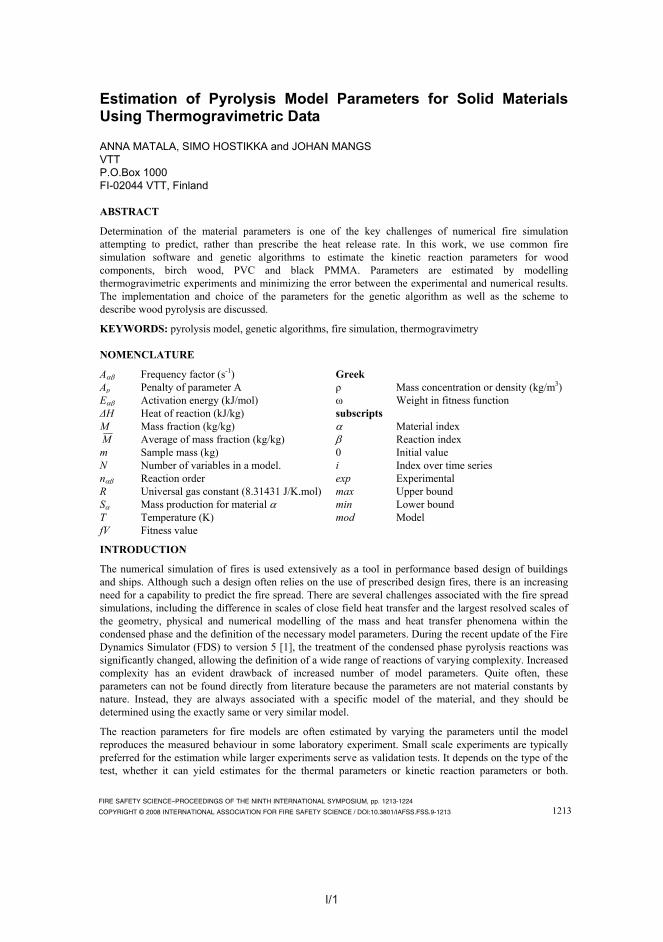
I/2 I/3

RTEn

seATr

αβαβ

ρρα

αβαβ−

⎟⎟⎠

⎞⎜⎜⎝

⎛=

0)( (2)

where ρα is the mass concentration of component α and ρs0 the original density of the material. The rate of change for the mass concentration of component α is

αβ

αβα

ρρ

Srt s

+−=⎟⎟⎠

⎞⎜⎜⎝

⎛∂∂ ∑

0 (3)

where Sα is the production rate of material α. is In words, the mass is consumed by all the reactions converting material α to something else and created by the reactions converting something else to α. If none of the reactions leaves solid residue, the sample volume is reduced correspondingly, thus retaining constant density.

Kinetic parameters A, E and n depend both on the material and the assumed reaction scheme. They must be determined using some sort of experimental data. To estimate the kinetic parameters for Eq. (1), a numerical model of the TGA experiment was created using Fire Dynamic Simulator (FDS) version 5.0.2 [1]. The model is very simple, consisting of only few gas phase control volumes and a single surface element to describe the sample material. A thin layer of sample material is heated by radiation from the surroundings with linearly increased temperature. The layer is thin enough to remain in equilibrium with the surroundings with a tolerance of few Kelvins. Gas phase convection and reactions are neglected and the sample backing is adiabatic.

Correct interpretation of the model output is important when comparing the experimental results and model predictions. TGA results are presented as mass fractions M. The model, in turn, provides us with a sample density ρ which is sum of the individual mass concentrations. Direct comparison between M and ρ/ρ0 is possible if the sample volume does not change. For non-charring materials, such as PMMA, the sample volume is reduced and the mass fractions leading to ρ/ρ0 must be based on the initial sample volume.

Parameter estimation

The parameter estimation was performed by minimizing the error between a measured and simulated TGA result using Genetic Algorithm (GA) as a minimization technique. GA was chosen because it is effective for problems with several unknown variables, and can usually find a global minimum instead of converging to some local minimum. Recently, GA has been used for the parameter estimation of condensed phase reactions by Lautenberger et al. [2] and Rein et al. [3].

Genetic algorithms are based on the idea of evolution and the procedure and the terminology is adapted from references [2], [3] and [5]. The process is iterative, and each iteration round corresponds to one generation. The first generation is initialized by generating random numbers for candidate solutions (individuals). An individual is a vector with real numbers corresponding to the unknown variables of the model. The individuals of a generation form a population. Population can be divided from the beginning into smaller subpopulations to keep up the variety of candidate solutions. Each generation goes through several processes. First, the goodness of an individual is tested using a fitness function returning a fitness value. According the fitness value, the individuals are ranked, and the best of them are selected to produce offspring. The offspring are formed by crossover, where the chosen individuals are set to pairs and each pair are changing alleles (values of variables) according the conditions of crossover. After that occur mutations, stochastically according to a predetermined mutation rate. In mutation, one value in an individual is replaced by a new random number. Then fitness values are calculated for the offspring and the best parents and offspring are chosen to the next generation. If population is divided into isolated subpopulations, some individuals migrate then between subpopulations bringing new genes and so maintaining variety. After each generation, the best individual is plotted, which enables the user to observe the action of algorithm. The process is repeated until the maximum number of iterations is finished or the user is satisfied with the result and stops the algorithm from outside.

1215

Mathematically, the parameter estimation process can be presented as an optimization problem. In the recent papers of Lautenberger et al. [2] and Rein et al. [3], Genetic Algorithms (GA) were used for the optimization to estimate the thermal material properties from bench scale experiments [2] and kinetic parameters from thermogravimetric experiments [3]. In this work, we use the ideas of the above mentioned authors to determine the kinetic reaction parameters for the modelling of pyrolysis behaviour of selected solid materials, including wood and its components, polyvinylchloride (PVC) and polymethyl methacrylate (PMMA). The reactions are modelled using FDS and the practical aspects associated with the use of genetic algorithms are studied.

METHODS

Experiments

In this work, the kinetic parameters of selected solid materials were determined using Thermogravimetric Analysis (TGA) [4]. In addition, Differential Scanning Calorimetry (DSC) was used to determine the heat of reaction. In both experiments, just 10-50 mg of sample material is needed. A small furnace is heated at constant heating rate (heating rate typically 2-20 K/min) so that the temperature of the sample is in equilibrium with the environment all the time. The purge gas can be air or nitrogen (N2). These thermoanalytical experiments were carried out at the Laboratory of Inorganic and Analytical Chemistry, Helsinki University of Technology, using Netzsch STA 449C equipment. The sample materials are listed in Table 1.

TGA measures the sample mass as a function of temperature. In this paper, the results are presented as a fraction of the current mass to the initial mass

0mmM = (1)

The main difference between TGA experiments conducted in air and in N2 is that in air, direct oxidation reactions may take place parallel or after the pyrolysis reaction. Oxidation decreases the mass of material, so the residual mass is usually smaller in air than in N2. This is true for all the sample materials discussed in this work. In DSC, temperature of a sample is kept identical with reference sample and the energy needed for that is measured. In DSC data it is possible to see if the reaction is endothermic or exothermic. Sometimes it is even possible to measure the heat of reaction by integrating over the peak in the DSC curve. Nitrogen should be used as a purge gas if the heat of reaction is going to be measured. However, sometimes many parallel reactions take place simultaneously or the measurement is not accurate enough, and the DSC graph does not give the expected results.

Table 1. Sample properties. The moisture-% is wet based.

Material Description ρ (kg/m3)

Moisture- %

Cellulose (Avicel® PH-101) High purity cellulose powder. 360 4 Lignin (alkali) Powder, 4 % sulphur, carbon typically 45 % - 65 % 494 8 Xylan from birch wood Powder, xylose residues ≥90 % 312 7 Birch - 550 3 PVC Almost pure PVC pipe material. 1440 0 Black PMMA ICI, Perspex 1180 0

Kinetic modelling of pyrolysis reactions

The condensed phase materials are modelled as mixtures of material components. In the modelling of condensed phase reactions, the rate of an individual condensed phase reaction β converting material α to something else is expressed as an Arrhenius equation

1214

I/3

RTEn

seATr

αβαβ

ρρα

αβαβ−

⎟⎟⎠

⎞⎜⎜⎝

⎛=

0)( (2)

where ρα is the mass concentration of component α and ρs0 the original density of the material. The rate of change for the mass concentration of component α is

αβ

αβα

ρρ

Srt s

+−=⎟⎟⎠

⎞⎜⎜⎝

⎛∂∂ ∑

0 (3)

where Sα is the production rate of material α. is In words, the mass is consumed by all the reactions converting material α to something else and created by the reactions converting something else to α. If none of the reactions leaves solid residue, the sample volume is reduced correspondingly, thus retaining constant density.

Kinetic parameters A, E and n depend both on the material and the assumed reaction scheme. They must be determined using some sort of experimental data. To estimate the kinetic parameters for Eq. (1), a numerical model of the TGA experiment was created using Fire Dynamic Simulator (FDS) version 5.0.2 [1]. The model is very simple, consisting of only few gas phase control volumes and a single surface element to describe the sample material. A thin layer of sample material is heated by radiation from the surroundings with linearly increased temperature. The layer is thin enough to remain in equilibrium with the surroundings with a tolerance of few Kelvins. Gas phase convection and reactions are neglected and the sample backing is adiabatic.

Correct interpretation of the model output is important when comparing the experimental results and model predictions. TGA results are presented as mass fractions M. The model, in turn, provides us with a sample density ρ which is sum of the individual mass concentrations. Direct comparison between M and ρ/ρ0 is possible if the sample volume does not change. For non-charring materials, such as PMMA, the sample volume is reduced and the mass fractions leading to ρ/ρ0 must be based on the initial sample volume.

Parameter estimation

The parameter estimation was performed by minimizing the error between a measured and simulated TGA result using Genetic Algorithm (GA) as a minimization technique. GA was chosen because it is effective for problems with several unknown variables, and can usually find a global minimum instead of converging to some local minimum. Recently, GA has been used for the parameter estimation of condensed phase reactions by Lautenberger et al. [2] and Rein et al. [3].

Genetic algorithms are based on the idea of evolution and the procedure and the terminology is adapted from references [2], [3] and [5]. The process is iterative, and each iteration round corresponds to one generation. The first generation is initialized by generating random numbers for candidate solutions (individuals). An individual is a vector with real numbers corresponding to the unknown variables of the model. The individuals of a generation form a population. Population can be divided from the beginning into smaller subpopulations to keep up the variety of candidate solutions. Each generation goes through several processes. First, the goodness of an individual is tested using a fitness function returning a fitness value. According the fitness value, the individuals are ranked, and the best of them are selected to produce offspring. The offspring are formed by crossover, where the chosen individuals are set to pairs and each pair are changing alleles (values of variables) according the conditions of crossover. After that occur mutations, stochastically according to a predetermined mutation rate. In mutation, one value in an individual is replaced by a new random number. Then fitness values are calculated for the offspring and the best parents and offspring are chosen to the next generation. If population is divided into isolated subpopulations, some individuals migrate then between subpopulations bringing new genes and so maintaining variety. After each generation, the best individual is plotted, which enables the user to observe the action of algorithm. The process is repeated until the maximum number of iterations is finished or the user is satisfied with the result and stops the algorithm from outside.

1215

I/4 I/5

Fig. 1. TGA graphs of same kinetic parameters with different heating rates.

The Genetic Algorithm application was implemented using Genetic Algorithm Toolbox for Matlab, developed by the Department of Automatic Control and Systems Engineering of The University of Sheffield, UK [6]. The toolbox is available for free at http://www.shef.ac.uk/acse/research/ecrg/getgat.html. The parameters used in the estimation are listed in Table 2. Many different combinations were studied and the listed parameters were found to give the best results in estimation of kinetic parameters. The variable and function names are consistent with the Genetic Algorithm toolbox.

Despite the simplicity of the FDS model used for TGA simulation, the computational cost of the parameter estimation was quite high because the model had to be solved for every individual of every generation, and with each heating rate separately. Estimations for this work took from about 10 h to one day to run on a single CPU of a modern workstation.

Table 2. Parameters of Genetic Algorithm application.

Parameter Symbol in GA Toolbox

Value

Number of individuals. NIND 20 Generation gap: The fractional difference between the new and old population sizes.

GGAP 0.8

Crossover rate. XOVR 0.7 Mutation rate. MUTR 1/Number of variables Maximum number of generations. MAXGEN 1200 Insertion rate: Fraction of offspring reinserted into the population.

INSR 0.9

Number of subpopulations. SUBPOP 4 Migration rate. MIGR 0.2 Number of genes per migration. MIGGEN 20

1217

The fitness function compares experimental data to model and returns a metrics of how good is the fit. This is often made by using least mean squares. Based on the numerical experiments, another feature was added to the fitness function: The results of the parameter estimation process are not unambiguous and several well-fitting parameters can be found for the same material. On the other hand, high values of pre-exponential factors A were found to make the FDS simulations more prone for numerical fluctuations. An additional term was thus added to the fitness function to prefer the smaller values of A. The formula for the fitness value is

( ) ( )

( ) p

i

i i AMM

MMMMfV 22

expexp

2modexp

2expexp

1 1 ωω +

⎟⎟⎟⎟⎟

⎠

⎞

⎜⎜⎜⎜⎜

⎝

⎛

−

−−−

−=∑

∑ ∑ (4)

where M is mass fraction in TGA experiment and i goes over all the data. ω1 and ω2 are the weights of fitness function so that ω1+ω2 =1. Ap is the penalty of high parameter A, and has a form

max

min

AAA

Ap−

= (5)

where A is the current value of the pre-exponential factor, Amin is its lower bound and Amax the upper bound. Weight ω2 should be in same order of magnitude as the differences in the fitness values of the best solutions. In the tests, these differences were around 15/1000. Too high weight would lead to small pre-exponential factors giving inaccurate predictions.

The population size and the division of one big population into smaller subpopulations are important when fast convergence to a possible local minimum must be avoided. Inside one population, the solution converges quite fast towards the best candidate solution. If there are many independent populations, the probability that one of the solutions is near the global minimum, is much higher. In test simulations, division to subpopulations was found to be even more important than the population size. The populations without separation converged very fast, no matter how big the number of individuals was in the population. On the other hand, when there were at least four subpopulations, each of them could have as few as 20 individuals and the diversity was still maintained well enough. Mutation rate is used to control the maintenance of diversity. It expresses the probability of an individual to mutate during one generation. If the mutation rate is too low, the solution may converge to a local minimum, and if it is too high, good solutions may be lost. A good rule of thumb is to choose a mutation rate close to ratio 1/N, where N is number of variables.

When TGA experiments are available at many different heating rates, the fitness value should be calculated considering all the rates, thus ensuring that the model is good in general, not only with one heating rate. To illustrate this, in Fig. 1 is shown a comparison of measured (solid lines) and simulated (dash lines) TGA results. The simulation used kinetic parameters that provided very good results at 2 K/min heating rate but poor predictions of the residue mass at others.

1216

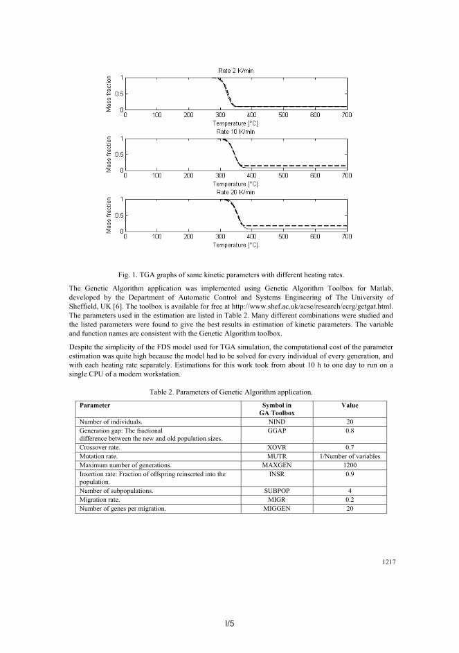
I/5

Fig. 1. TGA graphs of same kinetic parameters with different heating rates.

The Genetic Algorithm application was implemented using Genetic Algorithm Toolbox for Matlab, developed by the Department of Automatic Control and Systems Engineering of The University of Sheffield, UK [6]. The toolbox is available for free at http://www.shef.ac.uk/acse/research/ecrg/getgat.html. The parameters used in the estimation are listed in Table 2. Many different combinations were studied and the listed parameters were found to give the best results in estimation of kinetic parameters. The variable and function names are consistent with the Genetic Algorithm toolbox.

Despite the simplicity of the FDS model used for TGA simulation, the computational cost of the parameter estimation was quite high because the model had to be solved for every individual of every generation, and with each heating rate separately. Estimations for this work took from about 10 h to one day to run on a single CPU of a modern workstation.

Table 2. Parameters of Genetic Algorithm application.

Parameter Symbol in GA Toolbox

Value

Number of individuals. NIND 20 Generation gap: The fractional difference between the new and old population sizes.

GGAP 0.8

Crossover rate. XOVR 0.7 Mutation rate. MUTR 1/Number of variables Maximum number of generations. MAXGEN 1200 Insertion rate: Fraction of offspring reinserted into the population.

INSR 0.9

Number of subpopulations. SUBPOP 4 Migration rate. MIGR 0.2 Number of genes per migration. MIGGEN 20

1217

I/6 I/7

Fig. 2. TGA models of components of wood in N2. Heating rate is 2 K/min.

Birch

Birch is typical Finnish hardwood specie. When the temperature rises, the moisture of wood evaporates [8]. After this, the fibres start to degrade. The volatiles are now generated, and they consist of a combustible mixture of gases, vapours and tars. A solid carbon char matrix remains, and its volume is smaller than original volume of wood. The sample density was 550 kg/m3, which is higher than any of the component densities studied above. That is because the powders form of component samples.

For modelling the pyrolysis of birch four different schemes were used: Scheme 1 was a sum of the one-step reactions of components (cellulose, hemicellulose and lignin) yielding independently certain amount of char. Besides of char, fuel gases are released. In this scheme, the mass fractions of the component variables were also estimated using GA, in order to achieve the total density of birch. Scheme 2 was a one-step reaction converting virgin solid to char. Schemes 3 and 4 were presented by Liu et al. in Ref. [9]. In Scheme 3, there are two separate pseudo-components, which both produce char and fuel gases in parallel. In Scheme 4, there is only one material that has two consecutive reactions. The reaction formulas are summarized in Fig. 3.

1219

RESULTS Heats of reaction were achieved by integrating the reaction peaks of DSC data in nitrogen. Heat of reaction ΔH is the integral divided by consumed mass. Consistent values of ΔH were obtained at all the heating rates only for cellulose and birch. The value for cellulose was -482 kJ/kg and for birch -230 kJ/kg. Negative sign here means endothermic reaction. For comparison, di Blasi [7] has used ΔH = -418 kJ/kg for lignocellulosic fuel, which is relatively close to the value obtained here. However, it is considerably different from our value for birch.

The kinetic parameters of several materials were estimated using genetic algorithm. TGA experiments were made in nitrogen (N2) because the focus was on the modelling of the pyrolysis (degradation) reactions. For each of the kinetic parameters, a range of possible values was defined, as shown in Table 3. The ranges can be chosen according the literature values, if available, or initial estimates. In the tests, the ranges were set unnecessarily wide on purpose to be able to study the variety of solutions. Unfortunately, the choice of the range may affect the results, as was demonstrated by running two version of the black PMMA with different bounds for the reaction order n. Experimental results at four different heating rates (2, 5, 10 and 20 K/min) were used for the estimation. The iterations normally converged during the first 50 generations, but often the iteration process was continued at least up to 100, sometimes even 1000 generations. Most of the materials include some amount of moisture, and the evaporation of water was modelled as a one step reaction with own kinetic parameters. The numerical results are presented in Table 5 and as model behaviour in figures below.

Table 3. Estimation ranges for sample materials.

Material A (s-1) E (kJ/mol) n residue

Cellulose [1010,1020] [100,300] [0,7] [0,1]

Lignin (alkali) [1010,1020] [100,300] [0,7] [0,1]

Xylan from birch wood [1010,1020] [100,300] [0,7] [0,1]

Birch (all reactions) [1010,1020] [100,300] [0,5] [0,1]

PVC (all reactions) [108,1020] [100,300] [0,4] [0,1]

Black PMMA –estimation 1 [102,1010] [100,300] [0,2] -

Black PMMA –estimation 2 [102,1010] [100,300] [0,7] -

Components of wood

The three main components of wood are cellulose, hemicellulose and lignin. Roughly 40-44 % of hardwood is cellulose, 23-40 % hemicellulose and 18-25 % lignin [8]. All the components of wood produce char in combustion but lignin yields most of the char. The sample of hemicellulose was xylan, which is dominant hemicellulose specie in birch wood. The samples of components were in powder form, so the densities and thermal characteristics may differ from real. However, the kinetics’ were assumed to be the same. Cellulose was modelled using di Blasi’s model [7] and simple one-step model. The di Blasi model was slightly more accurate, but did not differ from the one-step model significantly. For other components, simple one-step reactions were assumed. With lignin and xylan, the experimental TGA data is not the best possible: Unexpected mass losses in the ends of the graphs are seen, which makes it more difficult to decide the residual mass. The results at 2 K/min heating rate are shown in Fig. 2. All the models succeed to predict the total mass loss quite well and the reactions take place in correct temperature range. The dominant shapes of graphs are correct but small errors can be found close to the end of the pyrolysis period. The numeric values of the kinetic parameters are given in Table 5.

1218

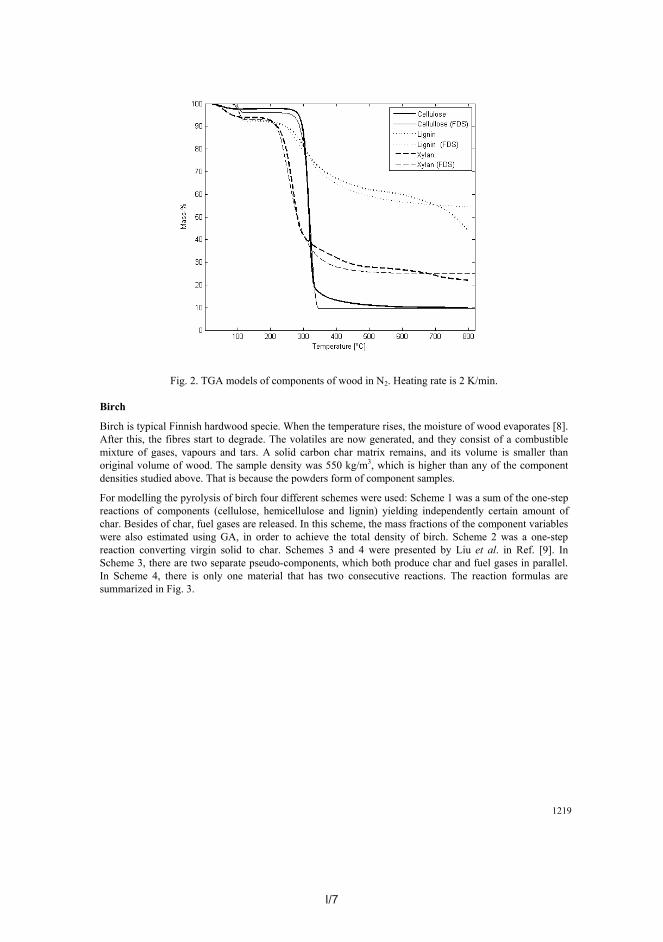
I/7

Fig. 2. TGA models of components of wood in N2. Heating rate is 2 K/min.

Birch

Birch is typical Finnish hardwood specie. When the temperature rises, the moisture of wood evaporates [8]. After this, the fibres start to degrade. The volatiles are now generated, and they consist of a combustible mixture of gases, vapours and tars. A solid carbon char matrix remains, and its volume is smaller than original volume of wood. The sample density was 550 kg/m3, which is higher than any of the component densities studied above. That is because the powders form of component samples.

For modelling the pyrolysis of birch four different schemes were used: Scheme 1 was a sum of the one-step reactions of components (cellulose, hemicellulose and lignin) yielding independently certain amount of char. Besides of char, fuel gases are released. In this scheme, the mass fractions of the component variables were also estimated using GA, in order to achieve the total density of birch. Scheme 2 was a one-step reaction converting virgin solid to char. Schemes 3 and 4 were presented by Liu et al. in Ref. [9]. In Scheme 3, there are two separate pseudo-components, which both produce char and fuel gases in parallel. In Scheme 4, there is only one material that has two consecutive reactions. The reaction formulas are summarized in Fig. 3.

1219

I/8 I/9

Fig. 4. TGA models of birch in N2. Heating rate is 2 K/min.

Fig. 5. TGA model of PVC in N2.

1221

Fig. 3. Reaction schemes for birch.

A comparison of the measured and predicted TGA curves at 2 K/min heating rate is shown in Fig. 4, and the fitness values corresponding to the last iteration are listed in Table 4. In scheme 1, the best model had the composition 44 % cellulose, 18 % lignin and 38 % xylan. Other parameters are listed in Table 5. According to a visual comparison and the fitness values, Scheme 2 gives the best prediction of the TGA curve, which suggests that the components in wood are behaving like a homogenous solid material rather than a mixture of three. Scheme 1 gave the worst results of all the studied schemes, and its fitness value was more than 10 times the fitness value of Scheme 2.

Table 4. Fitness values of TGA results of birch schemes.

Scheme 1 2 3 4 Fitness value 0.0691 0.0069 0.0119 0.0123

PVC

The sample was almost pure polyvinyl chloride (PVC) pipe material. PVC undergoes two reactions: Release of hydrochloric acid between 200 and 300°C and the pyrolysis reaction of the remaining solid at about 400°C. The pyrolysis products are HCl, benzene and toluene [8]. Reactions were modelled by two pseudo-components, of which the first does not yield any tar and the second does.

The mass fraction of volatiles was assumed to be 0.54 (taken directly from the graphs). A comparison of the measured and predicted TGA curves at the end of the parameter estimation is shown in Fig. 5. The solid lines denote the experimental data and the dash lines the model. Good predictions of the PVC pyrolysis are achieved at all heating rates. The numeric values of the kinetic parameters are given in Table 5.

Black PMMA

PMMA (Polymethyl methacrylate) is a non-charring thermoplastic that melts and then burns. The pyrolysis product is 100 % monomer [8] with no significant residue yield. Different from charring materials where the density decreases, in PMMA model the sample thickness decreases instead. This may cause problems when modelling TGA test where the sample is very thin from the beginning. As a result, care must be taken to define a sufficiently high sampling frequency for the numerical results.

1220

I/9

Fig. 4. TGA models of birch in N2. Heating rate is 2 K/min.

Fig. 5. TGA model of PVC in N2.

1221

I/10 I/11

Table 5. Kinetic parameters of materials, estimated using genetic algorithm.

Material A (s-1) E (kJ/mol) n residue Moisture 1·1020 162 1 0 Cellulose 2.68·1014 195 0.85 0.1 Lignin 2.18·1010 138 7 0.567 Xylan 5.78·1013 164 4.166 0.268 Birch – scheme 2 7.51·1011 161 3.12 0.172 Birch – scheme 3 – k1 8.64·1016 230 1 0.19 Birch – scheme 3 – k2 1.3·1012 150 1 0.19 Birch – scheme 4 – k1 9.26·1018 142 1 1 Birch – scheme 4 – k2 3.91·1010 148 1 0.268 Birch – scheme 4 – k3 1.05·1014 210 1 0 PVC (chlorides) k1 6.12·1016 198 2.18 0 PVC (solid) k2 3.63·1013 219 2.08 0.589 Black PMMA – estimation 1 2.43·109 146 1.758 0 Black PMMA – estimation 2 1.35·109 143 4.01 0

ACKNOWLEDGMENT

We thank Dr. Tuula Leskelä of Helsinki University of Technology (TKK), for performing the thermoanalytical experiments. This work was funded by the State Nuclear Waste Management Fund (VYR).

REFERENCES

[1] McGrattan, K., Hostikka, S., Floyd, J., Baum, H. and Rehm, R. Fire Dynamics Simulator (Version 5) Technical Reference Guide. National Instititute of Standards and Technology, MD. USA. NIST Special Publication 1018-5. 86 p. (Draft: August 26, 2007).

[2] Lautenberger, C., Rein, G., Fernandez-Pello, C., (2006). The application of a genetic algorithm to estimate material properties for fire modeling from bench-scale fire test data. Fire Safety Journal 41: 204-214. doi:10.1016/j.firesaf.2005.12.004

[3] Rein, G., Lautenberger, C., Fernandez-Pello, C., Torero, J., Urban, D., (2006). Application of genetic algorithms and thermogravimetry to determine the kinetics of polyurethane foam in smoldering combustion. Combustion and Flame 146: 95-108. doi:10.1016/j.combustflame.2006.04.013

[4] Kellner, R., Mermet J.-M., Otto, M., Valcárcel, M., Widmer, H. M., Analytical Chemistry: A Modern Approach to Analytical Science, Second editition. Wiley-VCH Verlag GmbH & Co. KGaA, Weinheim, 2004.

[5] Reeves, Colin R., Rowe, Jonathan E., Genetic algorithms - principles and perspective. Kluwer Academic Publishers. Kluwer Academic Publishers, 2002.

[6] Chipperfield, A., Fleming, P., Pohlheim, H., Fonseca, C. Genetic Algorithm Toolbox for Use with Matlab. Version 1.2. User’s Guide. Department of Automatic Control and Systems Engineering, University of Sheffield.

[7] Di Blasi, C., (1998) Physico-chemical processes occurring inside a degrading two-dimensional anisotropic porous medium. International Journal of Heat and Mass Transfer 41: 4139-4150. doi:10.1016/S0017-9310(98)00142-2

[8] Harper, C. (ed.) Handbook of building materials for fire protection. McGraw-Hill Handbooks. The McGraw-Hill Companies Inc., 2004.

[9] Liu, N., Chen, H., 2007. Two-step kinetic models for thermal decomposition of forest combustibles: Three kinetic schemes. 7th Asia-Oceania Symposium on Fire Science and Technology, Hong Kong.

1223

The estimation was made twice using different range for the reaction order parameter n. In the first run, the range was [0, 2] and in the second, it was [0, 7]. The result of estimation run 1 is shown in Fig. 6. Again, the solid line denotes the experimental data and the dash line the model. An accurate prediction of the mass loss is achieved at heating rates 5 and 10 K/min, and reasonably well at heating rates 2 and 20 K/min. The results of the estimation run 2 look very much the same and the model is considered as accurate as in estimation run 1. That suggests that the parameter sets can be chosen among various alternatives and the genetic algorithm can find solutions from desired range. The numeric values of the kinetic parameters are given in Table 5.

Fig. 6. TGA of black PMMA in N2.

CONCLUSIONS

Kinetic pyrolysis model parameters were estimated for six different solid materials using FDS fire model and genetic algorithm for the estimation. The estimation parameters, such as variable bounds and time step size, were carefully chosen to minimize the effect of the estimation procedure. The results were promising and indicated that the thermogravimetric experiments and genetic algorithm can successfully be used for the parameter estimation in fire engineering. As the material models were created using the actual fire simulation tool, the results can be directly used in applications. The estimation process is computationally expensive, taking several hours to a day on a single computer, but needs to be performed only once for each material. Validation of the current parameters and estimation of the lacking ones is still needed to build a full parameter set for fire spread computation.

Different reaction schemes were considered for the hardwood charring process. Best results were obtained using a simple one-step reaction for the pyrolysis. From the engineering viewpoint this is a very good result because the model simplicity means smaller number of unknown parameters to estimate and computational savings. Some of the resulting parameter values were quite different from those previously presented in literature. This demonstrates that the kinetic parameters are model dependent and should not be considered as fundamental material properties. The parameters should therefore be used only in models with similar structure. In addition, the estimation results are not unambiguous and there may be many suitable sets of parameters that predict the mass loss accurately.

1222

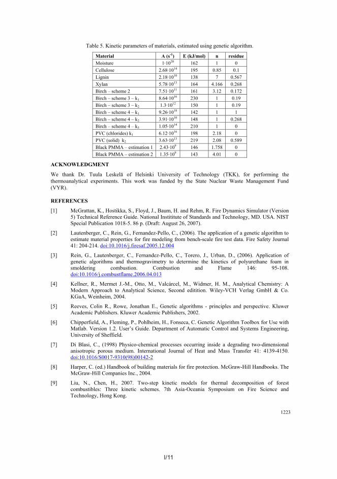
I/11

Table 5. Kinetic parameters of materials, estimated using genetic algorithm.

Material A (s-1) E (kJ/mol) n residue Moisture 1·1020 162 1 0 Cellulose 2.68·1014 195 0.85 0.1 Lignin 2.18·1010 138 7 0.567 Xylan 5.78·1013 164 4.166 0.268 Birch – scheme 2 7.51·1011 161 3.12 0.172 Birch – scheme 3 – k1 8.64·1016 230 1 0.19 Birch – scheme 3 – k2 1.3·1012 150 1 0.19 Birch – scheme 4 – k1 9.26·1018 142 1 1 Birch – scheme 4 – k2 3.91·1010 148 1 0.268 Birch – scheme 4 – k3 1.05·1014 210 1 0 PVC (chlorides) k1 6.12·1016 198 2.18 0 PVC (solid) k2 3.63·1013 219 2.08 0.589 Black PMMA – estimation 1 2.43·109 146 1.758 0 Black PMMA – estimation 2 1.35·109 143 4.01 0

ACKNOWLEDGMENT

We thank Dr. Tuula Leskelä of Helsinki University of Technology (TKK), for performing the thermoanalytical experiments. This work was funded by the State Nuclear Waste Management Fund (VYR).

REFERENCES

[1] McGrattan, K., Hostikka, S., Floyd, J., Baum, H. and Rehm, R. Fire Dynamics Simulator (Version 5) Technical Reference Guide. National Instititute of Standards and Technology, MD. USA. NIST Special Publication 1018-5. 86 p. (Draft: August 26, 2007).

[2] Lautenberger, C., Rein, G., Fernandez-Pello, C., (2006). The application of a genetic algorithm to estimate material properties for fire modeling from bench-scale fire test data. Fire Safety Journal 41: 204-214. doi:10.1016/j.firesaf.2005.12.004

[3] Rein, G., Lautenberger, C., Fernandez-Pello, C., Torero, J., Urban, D., (2006). Application of genetic algorithms and thermogravimetry to determine the kinetics of polyurethane foam in smoldering combustion. Combustion and Flame 146: 95-108. doi:10.1016/j.combustflame.2006.04.013

[4] Kellner, R., Mermet J.-M., Otto, M., Valcárcel, M., Widmer, H. M., Analytical Chemistry: A Modern Approach to Analytical Science, Second editition. Wiley-VCH Verlag GmbH & Co. KGaA, Weinheim, 2004.

[5] Reeves, Colin R., Rowe, Jonathan E., Genetic algorithms - principles and perspective. Kluwer Academic Publishers. Kluwer Academic Publishers, 2002.

[6] Chipperfield, A., Fleming, P., Pohlheim, H., Fonseca, C. Genetic Algorithm Toolbox for Use with Matlab. Version 1.2. User’s Guide. Department of Automatic Control and Systems Engineering, University of Sheffield.

[7] Di Blasi, C., (1998) Physico-chemical processes occurring inside a degrading two-dimensional anisotropic porous medium. International Journal of Heat and Mass Transfer 41: 4139-4150. doi:10.1016/S0017-9310(98)00142-2

[8] Harper, C. (ed.) Handbook of building materials for fire protection. McGraw-Hill Handbooks. The McGraw-Hill Companies Inc., 2004.

[9] Liu, N., Chen, H., 2007. Two-step kinetic models for thermal decomposition of forest combustibles: Three kinetic schemes. 7th Asia-Oceania Symposium on Fire Science and Technology, Hong Kong.

1223

I/12 13

13

PUBLICATION II

Generalized direct method for pyrolysis kinetic parameter

estimation and comparison to existing methods

In: Journal of Fire Sciences, Vol. 30, No. 4, pp. 339–356.

Copyright 2012 the Authors.Reprinted with permission from the publisher.

II/1

Article

Journal of Fire Sciences

30(4) 339–356

� The Author(s) 2012

Reprints and permissions:

sagepub.co.uk/journalsPermissions.nav

DOI: 10.1177/0734904112439840

jfs.sagepub.com

Generalized direct method forpyrolysis kinetic parameterestimation and comparison toexisting methods

Anna Matala1, Chris Lautenberger2 and Simo Hostikka1

Date received: 04 November 2011; accepted: 01 February 2012

AbstractSolid-phase pyrolysis is often modelled using the Arrhenius degradation equation with threeunknown parameters: reaction order, activation energy and pre-exponential factor. Since theparameters are model dependent and not directly measurable, several estimation methods havebeen developed over the years for extracting them from the experimental small-scale data. Lately,the most commonly used methods have been based on optimization and curve fitting. Thesemethods are very efficient for complex problems with multiple reactions but may require signifi-cant computational time. Direct (analytic) methods are simpler and faster but often have morerestrictions and limited accuracy. This article presents a new, generalized direct method and itsperformance evaluated along with other commonly used estimation methods. The real usability ofthe methods is tested also in the presence of small noise.

KeywordsPyrolysis, modelling, parameter estimation

Introduction

Solid-phase pyrolysis is often modelled using the Arrhenius reaction rate equation with threeunknown, model-specific parameters. These parameters are called kinetic parameters as theydefine the reaction kinetics. Direct measurement of these parameters using any commonexperimental apparatus is not possible. Knowing the reaction chemistry helps to define thereaction path but for an engineering solution, this may be far too complicated and

1VTT Technical Research Centre of Finland, FI-02044 VTT, Finland2Reax Engineering Inc., Berkeley, CA, USA

Corresponding author:

Anna Matala, VTT Technical Research Centre of Finland, PO Box 1000, Espoo, FI-02044 VTT, Finland.

Email: [email protected]

II/2 II/3

ambitious. In real pyrolysis, several reactions occur simultaneously and may overlap in timeand temperature. From the fire modeller’s point of view, it is not necessary or even worth-while to describe all those reactions but rather approximate the process using as few and assimple reactions as possible. It is a well-known fact that the model parameters are able tocompensate the other shortcomings and simplifications in the model.1,2 As the kinetic para-meters are associated with a specific reaction scheme having no fundamental physical signifi-cance, their values can indeed be chosen freely in order to get the best possible descriptionof reality using the model in hand.

For obtaining the kinetic parameters, one needs to extract them from small-scale experi-mental data. The most commonly used small-scale experiment is non-isothermal thermogra-vimetric analysis (TGA), which measures the loss of a very small (few milligrams) sampleduring constant rate heating. There are basically two approaches to property estimation:curve fitting (mainly evolutionary algorithms)3–8 and analytical methods.8–11 Both have theiradvantages: curve fitting has very few limitations related to the reaction path or estimatedparameters and can operate very effectively for complicated, overlapping reactions andnoisy data. Their shortcoming is that they often require significant computational time forthe iteration process to converge and some specific software for performing the estimation.It may also be discomforting that – due the compensation effect and other factors – severalequally fitting solutions may be found (meaning the solution is not unique). Furthermore,the process is stochastic, which means that the results and the estimation routine cannot berepeated with exactly same results. Analytical methods, on the other hand, use referencepoints (such as the peak reaction rate) in experimental data to define kinetic parameters.They do operate well for simple, non-noisy and non-overlapping data and give unique solu-tions without requiring lengthy iterations. They also require just a pencil and paper forobtaining the solutions, so they are fast and efficient solution for an engineer. However, theyare often limited to some specific reaction path and well-separated reactions. Noise in thedata can lead to difficulties.

In this work, a generalized direct (analytical) method (GDM) for estimating reactionkinetics from TGA data is presented and its performance is compared to alternative com-mon estimation methods. The methods are assessed in terms of accuracy of the results, timeconsumed and level of user participation and knowledge needed. All the simulations in thiswork have been made using the pyrolysis model of fire dynamic simulator (FDS) version6.0.0.12

Estimation methods

Direct method

The direct method (DM) considers a multiple step (k being the reaction index), Nth orderreaction path, where the reaction steps are well separated. By reactions being well separated,we mean that the reaction k 2 1 is completed before reaction k starts. This method is basedon the same idea as Friedman used for the one-step reaction.11 The char-yielding reaction ofconverting material A into material B and fuel gas is described as

A ! 1� vkð ÞB+ vkgas

for each reaction k. The conversion after the reaction k is defined as

340 Journal of Fire Sciences 30(4)

II/3

ak = 1�mk

m0

ð1Þ

where mk is the mass after reaction k is complete and m0 is the initial mass of the sample. Areaction progress variable a*

k corresponding to the mass released from one-step reaction canbe defined as

a�k =

a� ak�1

ak � ak�1

ð2Þ

An Arrhenius form of the decomposition reaction rate can be written for multiple reac-tions as

da�k

dt=Ak 1� a�

k

� �Nk exp � Ek

RT

� �ð3Þ

Replacing the reaction progress variable with the relation from equation (2) and dividingboth sides by the heating rate b= dT=dt, the Arrhenius equation becomes

da

dT=Ak

b

ak � að ÞNk

ak � ak�1ð ÞNk�1exp � Ek

RT

� �ð4Þ

To connect these analytical expressions to the thermogravimetric data, a reference pointneeds to be specified. In DM, the reference point for each of the reactions is chosen from thepeak of the differential thermogravimetric (DTG) curve, as shown in Figure 1. The first deri-vative (with respect to temperature) of the conversion at the reference point of kth reactionis called reference value and is denoted as rpk.

rpk [ maxda

dT

� �ð5Þ

Figure 1. Reference points of the direct methods.

Matala et al. 341

II/4 II/5

The corresponding temperature and conversion values are denoted as Tpk and apk, respec-tively. The second derivative of the conversion a is zero at reference point. Using these defi-nitions, we can solve the above equation for activation energy

Ek =NkRrpk

ak � apk

T2pk ð6Þ

Alternatively, the calculation can be made using the reference value based on the first timederivative of the conversion

Ek =NkR

b

max da=dtð Þak � apk

T2pk ð7Þ

By substituting the activation energy into equation (4), we obtain an equation for pre-exponential factor

Ak = rpkbak � ak�1ð ÞNk�1

ak � apk

� � expEk

RTpk

� �ð8Þ

Now, the only unknown parameter is the reaction order Nk. In certain applications, it canbe assumed to be one, but for more general approach, some methods from the literature arepresented. Gao et al.13 listed theoretical limits for the conversion as a function of the reactionorder. A very simple curve fit can be made for approximating the reaction order

Nk’13:25 1� a�p, k

� �3

� 4:16 1� a�p, k

� �2

+ 2:3 1� a�p, k

� �� 0:077 ð9Þ

where a*p is the reaction progress variable from equation (2) at the peak. More elaborate

methods have been presented by Friedman.11 For three different points (1, 2, 3) of a singleexperimental TGA curve, the reaction order can be calculated as

Nk =ln r3k

r1k

� �� T2k T3k�T1kð Þ

T3k T2k�T1kð Þ lnr2kr1k

� �

T2k T3k�T1kð ÞT3k T2k�T1kð Þ ln

1�a�1k

1�a�2k

� �� ln

1�a�1k

1�a�3k

� � ð10Þ

If one point is the peak value, N can be estimated using only two reference points (1, p)

Nk =ln

rpkr1k

� �

Tpk Tpk�T1kð ÞrTpT1 1�a�

pk

� � � ln1�a�

1k

1�a�pk

� � ð11Þ

Generalized Direct Method (GDM)

The DM is very sensitive to the correct definition of the conversion and the peak value. If thereactions are overlapping at later stage, it may be more convenient to choose the referencepoint where the reactions do not yet overlap. That is, either before or after the peak value. Ifthe reference point is chosen from where the third derivative is zero (see Figure 1), the activa-tion energy can be calculated as (neglecting the reaction index k for brevity)


II/5

E =�b6

ffiffiffiffiffiffiffiffiffiffiffiffiffiffiffiffiffiffib2 � 4ac

p

2að12Þ

where

a=ak�appð Þ2R2T4

pp

b= � 2rppNk ak�appð ÞRT2

pp� 2 ak�appð Þ2

RT3pp

c= r2pp Nk � 1ð ÞNk � rTppNk ak � app

� �

8>>><>>>:

Here Tpp is the reference point and rpp and rTpp are the first and second derivatives of theconversion at the reference point, respectively. The second gradient rT has two peaks and thesign (6) in equation (12) depends on which peak is chosen. If the first (positive) peak is cho-sen, the sign is positive. After this, Ak can be calculated at the point Tpp as in equation (8)and Nk as previously described for DM. This will be called GDM.

Data reduction

It is customary to perform the TGAs at different heating rates, typically between 1 and20 K/min. In fires, the heating rates can, at least for short periods of time, be as high as 1000K/min. In this work, some approaches to the reduction of the estimation results obtainedfrom different heating rates are studied. First of all, the results from all the heating ratesmust be somehow averaged for a general result. The averaging can be performed either tothe calculated parameter values (A, E, N) or to the reference values (a, T, r).

In addition, the effect of the heating rate range can be considered by giving more or lessimportance to the extreme heating rates. Different weighting methods examined are listed inTable 1.

The error (fitness value) between target and estimated curves is calculated as sum of errorsin conversions scaled by average relative deviation

fV =

Pj

amod, j � aexp , j

�� Pj

aexp , jð13Þ

with the summation going over the values obtained at different temperatures. Small fitnessvalue means good fit in this work.

Table 1. Weighting functions for different heating rates

wt1 wi =mPi

bi

(direct mean)

wt2 wi =1

bi�mj jPi

ibi�mj j

1 (heating rates near mean value get greater weight)

wt3 wi =bi�mj jP

i

bi�mj jð Þ (heating rates far from mean value get greater weight)

m is the mean of the heating rates.

Matala et al. 343

II/6 II/7

Other commonly used estimation methods

Several authors have proposed other analytical methods for obtaining the kinetic para-meters. Some of the methods are listed in Table 2. These methods are generally easy andquick to use, and they provide relatively unique solutions. Friedman developed his methodfor a single-step model, but here, it is scaled for multiple steps for generality. McGrattanet al. and Lyon et al.9,10 presented essentially the same equations with slightly different deri-vations and nomenclature. They both assumed first-order reaction kinetics. Lyon et al. addi-tionally limited the reaction path to just one reaction but offered an alternative method forextracting the reaction parameters using the heat release rate from microscale combustioncalorimeter (MCC).10,14 Those equations may have great value for some applications butare not evaluated here since they require different experimental apparatus than the othermethods.

Besides the analytical methods, several curve-fitting algorithms have been applied for thekinetic parameter estimation. Evolutionary algorithms are most commonly used, includinggenetic algorithms (GA),3–7 hybrid genetic algorithms (HGA)7 and shuffled complex evolu-tion (SCE).7,8 Their main idea is based on the survival of the fittest. The algorithm startsfrom a random set of trial solutions and tests their fitness against the experimental curve.The probability of the stochastic processes depends on this fitness value; the better the fitnessvalue, the greater the probability of the trial solution surviving to the next iteration round.Other processes are crossover (creating new trial solution by uniting two older solutions),mutation (one or more parameters are replaced by a random number) and migration (trialsolutions change place between two groups of the solutions). These algorithms are very effi-cient for complex problems with many parameters, overlapping reactions and even noisydata. They are a bit more complicated to use than the analytical methods and require signifi-cant amount of computer resources.

Results and discussions

Simple synthetic material

Four analytical methods, presented by equations (6) to (12) and Table 2, and two optimiza-tion methods (GA and SCE) were tested using a synthetic material sample with two

Table 2. Analytical methods used in this work

Method E A Values tospecify/reaction

Direct method Ek =NkRrpk

ak�apkT2pk Ak = rpkb

ak�ak�1ð ÞNk�1

ak�apkð ÞNk exp EkRTpk

� �5: rp, Tp, ap, ak, ak2 1

Generalizeddirect method

E= �b6ffiffiffiffiffiffiffiffiffiffiffib2�4ac

p

2a a, b and c asin equation (12)

Ak = rppkbak�ak�1ð ÞNk�1

ak�appkð ÞNk exp EkRTpp

� �6: rpp, rTpp, Tpp,app, ak, ak2 1

Friedman11

Ek = �Rln

r2kr1k

� �+Nk ln

ak�a1kak�a2k

� �1

T2k� 1

T1k

Ak =br1k ak�ak�1ð ÞNk�1

exp � ERT1k

� �ak�ak�1ð ÞNk

8: r1T, r2T, T1, T2, a1k,a2k, ak, ak2 1

McGrattan et al.8

and Lyon et al.10Ek =

RT2pkerpk

ak�ak�1N = 1 Ak =

berpkak�ak�1

exp EkRTpk

� �4: rp, Tp, a1k, ak2 1


II/7

well-separated reactions. The synthetic material was chosen because of known target values,simple shape and non-noisy data. The reaction path is shown in Figure 2. Two pseudocom-ponents are assumed with mass losses of 0.35 and 0.4, respectively, of the original mass, andthey were assumed to be known. The first reaction produces water vapour (as some flameretardants) and the second reaction produces fuel gas. The reaction order was calculatedusing equations (9) and (10) and assuming a first-order reaction for comparison for thosemodels that it was applicable.

The synthetic target data were generated for four different heating rates (5, 10, 30 and 50K/min), and the results were generalized using the weighting functions (Table 1) for eitherdirectly for the estimated parameter values or for the reference points and values. The realperformance of the parameters was then tested using target data at 20 K/min and 100 K/min.A summary of the test scheme is shown in Figure 3.

The parameter estimation produced in total 62 sets of kinetic parameters, and they weretested for two different heating rates (20 and 100 K/min). The predicted DTG curves withbest fitting parameter sets of each method are presented in Figure 4. In addition to theoverall result covering the whole temperature range (Figure 4(a)), the detailed results of

Figure 3. Test scheme for the estimation methods.DM: direct method; GDM: generalized direct method; GA: genetic algorithms; SCE: shuffled complex evolution.

Figure 2. Reaction path for the simple synthetic material.

Matala et al. 345

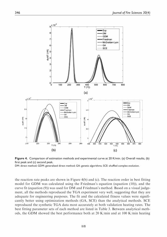
II/8 II/9

the reaction rate peaks are shown in Figure 4(b) and (c). The reaction order in best fittingmodel for GDM was calculated using the Friedman’s equation (equation (10)), and thecurve fit (equation (9)) was used for DM and Friedman’s method. Based on a visual judge-ment, all the methods reproduced the TGA experiment very well, suggesting that they areadequate for engineering purposes. The fit and the calculated fitness values were signifi-cantly better using optimization methods (GA, SCE) than the analytical methods. SCEreproduced the synthetic TGA data most accurately at both validation heating rates. Thebest fitting parameter sets of each method are listed in Table 3. Between analytical meth-ods, the GDM showed the best performance both at 20 K/min and at 100 K/min heating

Figure 4. Comparison of estimation methods and experimental curve at 20 K/min. (a) Overall results, (b)first peak and (c) second peak.DM: direct method; GDM: generalized direct method; GA: genetic algorithms; SCE: shuffled complex evolution.


II/9

Table

3.Bestfittingparam

eter

setsofeach

method

Target

values

DM,equations

(6)and(8)

GDM,equations

(8)and(12)

Friedman

(Table2)

McG

rattan

–Lyon

(Table2)

GA

SCE

A1(s21)

1.5031015

3.103

1014

4.113

1015

5.833

1014

2.673

1012

3.413

1015

1.4731015

E1(kJ/km

ol)

1.603

105

1.533

105

1.633

105

1.563

105

1.363

105

1.623

105

1.603

105

N1

1.50

1.43

1.50

1.43

1.00

1.59

1.50

A2(s21)

1.003

1012

2.483

1011

1.173

1012

3.153

1011

6.053

107

4.523

1011

9.933

1011

E2(kJ/km

ol)

2.103

105

2.033

105

2.123

105

2.053

105

1.513

105

2.053

105

2.103

105

N2

2.00

1.92

2.00

1.92

1.00

1.97

2.00

fV(20K/m

in)

20.0086

0.0070

0.0085

0.0299

0.0024

0.0003

fV(100K/m

in)

20.0111

0.0082

0.0109

0.0131

0.0041

0.0003

fV(H

RR)

20.0832

0.0591

0.0819

0.2463

22

fV(M

LR)

20.0045

0.0022

0.0047

0.0151

22

Number

ofreference

points(excludingN)

10

12

16

82

2

Comments

Ncfequation(9),

Ref.ave,wt3

Nfequation(10),

Ref.ave,wt2

Ncfequation(9),

Ref.ave,wt3

N=1,Par.ave,wt3

22

DM:directmethod;GDM:generalized

directmethod;G

A:geneticalgorithms;SC

E:shuffled

complexevolution;HRR:heatreleaserate;MLR

:massloss

rate.

‘Ref.ave’means

that

reference

values

wereaveraged.‘Par.ave’means

that

param

eterswereaveraged.Sm

allfitnessvaluemeansgoodfit.

Theusedreactionorder

Nandinform

ationabouttheparam

eter

averagingarelistedinthecomments(Table1).

Matala et al. 347

II/10 II/11

rates. McGrattan–Lyon method provided the fit with the largest error, but this is to beexpected since it is limited to first-order reactions. Of the other analytical methods, onlyFriedman’s method performed reasonably well when N = 1 was assumed.

The effects of the weight functions and two different means of averaging were examinedby calculating the fitness values for the validation results of each of the analytical methods.The fitness values with different weight functions are listed in Table 4. For all the othermethods except MGrattan–Lyon, the results were much more accurate when the referencevalues were first averaged prior to calculating the parameters. For the McGrattan–Lyonmethod, straight averaging of the parameters resulted in better fits. The different weightfunctions also had some significant effect on the resulting fitness values. Surprisingly, forDM and Friedman’s method, it seems that the wt2 (emphasizing the heating rates closer tomean value) has the better extrapolating ability than wt3 (emphasizing the heating rates farfrom mean value). For GDM, the opposite was true.

While the analytical methods were very quick to use, the optimization methodsrequired significant computational time even when parallel processing was used to speedup the computations. The set-up time for all the methods was more or less the same. Forthe analytical methods, the added complexity means increasing number of referencepoints to be chosen (listed in Table 2). The method of McGrattan and Lyon is the sim-plest with only four values to specify per reaction, while Friedman’s method is the mostcomplicated one with eight values per reaction. The curve fit reaction order (equation (9))requires only three reference points, while the Friedman’s equation (equation (10)) needseight. Of course, the use of the analytical methods could be automated reducing theworkload.

The significance of the differences in estimated kinetic parameters was studied byapplying the results of the analytical methods to a simulated cone calorimeter test. The

Table 4. Fitness values of the analytical methods with different weight functions

Averaging DM GDM Friedman McGrattan–Lyon

fV (20 K/min)

Parameters wt1 0.0236 0.0570 0.0174 0.0314wt2 0.0210 0.0536 0.0229 0.0316wt3 0.0182 0.0486 0.0207 0.0299

Reference values wt1 0.0100 0.0108 0.0099 0.0453wt2 0.0129 0.0070 0.0130 0.0409wt3 0.0086 0.0084 0.0085 0.0491

fV (100 K/min)

Parameters wt1 0.0311 0.0689 0.0227 0.0132wt2 0.0282 0.0638 0.0292 0.0131wt3 0.0250 0.0603 0.0267 0.0131

Reference values wt1 0.0128 0.0122 0.0123 0.0297wt2 0.0181 0.0082 0.0174 0.0242wt3 0.0111 0.0094 0.0109 0.0342

DM: direct method; GDM: generalized direct method.

The N is calculated as in Table 3.


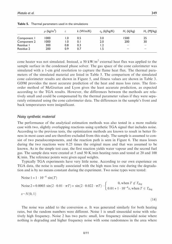
II/11

cone heater was not simulated. Instead, a 50 kW/m2 external heat flux was applied to thesample surface in the condensed phase solver. The gas space of the cone calorimeter wassimulated with a 1-cm grid resolution to capture the flame heat flux. The thermal para-meters of the simulated material are listed in Table 5. The comparison of the simulatedcone calorimeter results are shown in Figure 5, and fitness values are shown in Table 3.GDM provides the most accurate prediction of the heat and mass loss rates. The first-order method of McGrattan and Lyon gives the least accurate prediction, as expectedaccording to the TGA results. However, the differences between the methods are rela-tively small and could be compensated by the thermal parameter values if they were sepa-rately estimated using the cone calorimeter data. The differences in the sample’s front andback temperatures were insignificant.

Noisy synthetic material

The performance of the analytical estimation methods was also tested in a more realisticcase with two, slightly overlapping reactions using synthetic TGA signal that includes noise.According to the previous tests, the optimization methods are known to result in better fit-ness in most cases and are therefore excluded from this study. The sample is assumed to con-sist of two pseudocomponents, and the reaction path is seen in Figure 6. The mass lossesduring the two reactions were 0.25 times the original mass and that was assumed to beknown. As in the simple test case, the first reaction yields water vapour and the second fuelgas. The sample data were created at 5 and 50 K/min heating rates and tested at 20 and 100K/min. The reference points were given equal weights.

Typically TGA experiments have very little noise. According to our own experience onTGA data, the noise is usually associated with the high mass loss rate during the degrada-tion and is by no means constant during the experiment. Two noise types were tested:

Noise 1= 1 � 10�4 sin Tð Þ

Noise 2= 0:0003 sin 2 � 0:01 � pTð Þ+ sin 2 � 0:022 � pTð Þ �0,when T 62 Tdeg

0:01+ 1 � 10�4x,when T 2 Tdeg

�

x;N 0, 1ð Þð14Þ

The noise was added to the conversion a. It was generated similarly for both heatingrates, but the random numbers were different. Noise 1 is small sinusoidal noise with rela-tively high frequency. Noise 2 has two parts: small, low frequency sinusoidal noise wherenothing is degrading and higher frequency noise with some randomness in the area where

Table 5. Thermal parameters used in the simulations

r (kg/m3) e k (W/m/K) cp (kJ/kg/K) Hr (kJ/kg) Hc (MJ/kg)

Component 1 1000 1.0 0.5 3.0 1500 25Component 2 1000 1.0 0.1 2.0 200 30Residue 1 300 0.8 0.3 1.2 2 2Residue 2 200 0.9 0.7 1.5 2 2

Matala et al. 349

II/12 II/13

the sample is degrading. The noise levels can be seen in Figure 7. Noise 2 is significantlygreater than Noise 1, and it is based on an analysis of real, noisy TGA data. Fitness valueswere calculated compared to the original, non-noisy data. The noisy data were tested usingall the methods listed in Table 2. Due to the strong overlapping of the reactions, the reactionorder (N) could not be accurately calculated using the Friedman’s method, and therefore,the curve fit method in equation (9) was used for all methods.

The parameter estimation results are listed in Table 6 and visually presented for Noise 2in Figure 8. When no noise was added, all the methods where N 6¼ 1 predicted the DTGcurve very accurately. Small sinusoidal noise (Noise 1) did not cause significant error forDM or Friedman’s method, but for GDM, the error increased especially in the second peak.This is probably due to the fact that the magnitude of the error caused by the high-frequencynoise increases with each successive derivative, and therefore, small error in the mass datacauses greater error in the second derivative. It is also more difficult to define the location ofthe peak from very noisy data.

Noise 2 was more challenging for all other methods except GDM. The results are shownin Figure 8. The effect of the noise depends on the location of the greatest error, whether it is

Figure 5. Effect of different sets of kinetic parameters in cone calorimeter model at 50 kW/m2. (a) HRRand (b) MLR.DM: direct method; GDM: generalized direct method; HRR: heat release rate; MLR: mass loss rate.

Figure 6. Reaction path for slightly overlapping synthetic material.


II/13

located exactly at the reference point or not. In some cases, the noise can even improve theaccuracy of the method, as can be seen for the DM and Friedman’s method for Noise 1 at100 K/min, compared to the results without any noise. All the methods produced acceptableaccuracy for simulation purposes at both noise types.

The sets of kinetic parameters estimated with Noise 2 were tested in cone calorimeter at50 kW/m2 heat flux level. The simulations were made using 1 cm grid size. The thermalparameters were the same as for the simple test case (Table 5), and the heat release rate andmass loss rate at 50 kW/m2 are shown in Figure 9. The fitness values of the cone calorimeterresults with Noise 2 are listed in Table 6. Only the kinetic parameters estimated usingMcGrattan–Lyon method caused slightly higher rate and earlier flame out compared to thetarget results. As expected according to the TGA results, GDM provided the best fit also inthe cone calorimeter results. The significance of this difference is very small, as the thermalparameters are known to compensate the inaccuracies in the kinetic model. The kinetic para-meters did not have any significant effect on the front and back temperatures of the sample.

Summary and conclusions

A DM for estimation of kinetic parameters was generalized for multiple reactions and com-pared with other commonly used estimation methods. Both analytical methods and optimi-zation algorithms were compared. For analytical methods, different methods for calculatingthe reaction order were also presented and assessed and different weight functions for theheating rates tested. Synthetic experimental data based on known kinetic parameters wereused. The first test was a simple two-step reaction with well-separated reactions and no noise.

Figure 7. Noise 1 and Noise 2.

Matala et al. 351

II/14 II/15

Table

6.Target

1.50.101

52.00.1051.501.00.101

01.60.1052.00–Estimated

param

eterswhen

noiseisadded

tothesampledata

A1(s21)

E1(kJ/km

ol)

N1

A2(s21)

E2(kJ/km

ol)

N2

fV(20K/m

in)

fV(100K/m

in)

Nonoise

Target

1.5031015

2003

103

1.50

1.003

1010

1.603

105

2.00

––

DM

3.503

1014

1.923

105

1.35

6.653

1011

1.593

105

1.96

0.0104

0.0117

GDM

8.293

1014

1.963

105

1.35

7.253

1011

1.853

105

1.96

0.0105

0.0151

Friedman

6.193

1014

1.953

105

1.35

2.783

109

1.543

105

1.96

0.0103

0.0137

McG

rattan–Lyon

1.343

1013

1.753

105

1.00

4.553

106

1.173

105

1.00

0.0576

0.0465

Noise1

DM

5.593

1014

1.943

105

1.35

2.363

1010

1.663

105

2.01

0.0104

0.0100

GDM

5.293

1014

1.943

105

1.35

1.223

1017

2.553

105

2.01

0.0183

0.0314

Friedman

6.103

1014

1.953

105

1.35

8.923

109

1.603

105

2.01

0.0106

0.0119

McG

rattan–Lyon

2.193

1013

1.783

105

1.00

8.463

106

1.203

105

1.00

0.0578

0.0492

Noise2

DM

2.313

1015

2.013

105

1.45

5.073

1011

1.833

105

2.40

0.0169

0.0143

GDM

7.763

1014

1.963

105

1.45

1.673

1016

2.433

105

2.40

0.0120

0.0181

Friedman

1.253

1016

2.103

105

1.45

7.483

1012

1.983

105

2.40

0.0149

0.0093

McG

rattan–Lyon

1.793

1013

1.763

105

1.00

7.903

106

1.193

105

1.00

0.0634

0.0553

DM:directmethod;G

DM:generalized

directmethod.


II/15

Figure 8. Estimation results with different analytical methods for data with Noise 2 at 20 K/min. (a)Overall results, (b) first peak and (c) second peak.DM: direct method; GDM: generalized direct method.

Table 7. Fitness values of cone calorimeter results with Noise 2

fV (HRR) fV (MLR)

DM 0.0790 0.0032GDM 0.0386 0.0007Friedman 0.0629 0.0028McGrattan–Lyon 0.3166 0.0146

HRR: heat release rate; MLR: mass loss rate; DM: direct method; GDM: generalized direct method.

Matala et al. 353

II/16 II/17

The second test had two slightly overlapping reactions. Two types of noise were added to thedata for testing the performance in a more realistic case with experimental noise.

For the simple sample case, the parameters were estimated at four different heating ratesand then averaged using different weight functions. The results were then used at two otherheating rates to test the extrapolating ability of the results. Optimization methods turnedout to produce better fitting results, but all the methods, including the analytical methodswere able to find parameters that produce a sufficiently accurate fit for most engineeringapplications. The McGrattan–Lyon method was the simplest and fastest to use without anysoftware. All the analytical methods take just few minutes to obtain results, while the opti-mization methods take hours or days for running the algorithm.

The noisy sample was tested only using the analytical methods. The parameters were esti-mated at two heating rates, and the fitness of the solution was tested at two other heatingrates. Without noise, all the analytical methods, excluding the first-order McGrattan–Lyonmethod, reproduced the TGA results very accurately. In case of small high-frequency noise(Noise 1), most method still performed very well but the performance of the GDM wasgreatly hampered. In case of Noise 2, consisting of lower frequency components, the predic-tions were significantly less accurate for all the methods except for the GDM. The phase ofthe noise signal with respect to the selected reference points has somewhat random effect onthe performance of the estimation methods. In both test cases, the mass losses of the reac-tions were assumed to be known exactly. The uncertainties of the methods may be higher ifthe mass losses are also estimated from the experimental data.

The differences in the TGA predictions did not cause significant errors in the cone calori-meter scale. Furthermore, the thermal parameters are known to be able to compensate smalldifferences in the kinetic models, and therefore, the errors can be reduced if some of the ther-mal parameters are estimated using the cone calorimeter data itself.

This work demonstrates that the analytical methods can be used efficiently as substitutesto the computationally expensive optimization methods when estimating the parameters ofpyrolysis kinetics. There are several methods to choose from, and the choice depends on the

Figure 9. The performance of the estimation results in cone calorimeter model at 50 kW/m2. (a) HRRand (b) MLR.HRR: heat release rate; MLR: mass loss rate; DM: direct method; GDM: generalized direct method.


II/17

required accuracy, complexity and the experimental data. Methods with fewer reference val-ues work better in case of noisy data and overlapping reactions, while more complicatedmethods yield more accurate results for clean, simple data. Removing the high-frequencynoise from the mass data by filtering is recommended in order to improve the performanceof methods relying on higher-order derivatives of the mass data, such as the GDM.

Funding

The work of A. Matala and S. Hostikka was funded by the European Union under 7th Frameworkproject FIRE-RESIST and by the State Nuclear Waste Management Fund of Finland. The work of C.Lautenberger was funded by the National Science Foundation under Grant No. 0730556.

Conflict of interest

Any opinions, findings and conclusions or recommendations expressed in this material are those of theauthors and do not necessarily reflect the views of the National Science Foundation (NSF).

References

1. Nikolaev AV, Logvinenko VA and Gorbatchev VM.Special features of the compensation effect in non-isothermal kinetics of solid-phase reactions. J Therm Anal1974; 6: 473–577.

2. Matala A and Hostikka S. Pyrolysis modeling of PVCcable materials. Fire Saf Sci 2011; 10: 917–930.

3. Lautenberger C, Rein G and Fernandez-Pello C. Theapplication of a genetic algorithm to estimate materialproperties for fire modeling from bench-scale fire test data.Fire Safety J 2006; 41: 204–214.

4. Rein G, Lautenberger C, Fernandez-Pello C, et al.Application of genetic algorithms and thermogravimetryto determine the kinetics of polyurethane foam insmoldering combustion. Combust Flame 2006; 146: 95–108.

5. Matala A, Hostikka S and Mangs J. Estimation ofpyrolysis model parameters for solid materials usingthermogravimetric data. Fire Saf Sci 2009; 9: 1213–1223.

6. Lautenberger C and Fernandez-Pello C. Generalizedpyrolysis model for combustible solids. Fire Safety J 2009;44: 819–839.

7. Lautenberger C and Fernandez-Pello C. Optimizationalgorithms for material pyrolysis property estimation. FireSaf Sci 2011; 10: 751–764.

8. Chaos M, Khan MM, Krishnamoorthy N, et al.Evaluation of optimization schemes and determination ofsolid fuel properties for CFD fire models using bench-scalepyrolysis tests. P Combust Inst 2011; 33(2): 2599–2606.

9. McGrattan K, McDermott R, Mell W, et al. Modeling theburning of complicated objects using Lagrangian particles.In: Conference proceedings of the twelfth internationalinterflame conference, 2010, pp.743–753.

10. Lyon RE, Safronava N and Oztekin E. A simple methodfor determining kinetic parameters for materials in firemodels. Fire Saf Sci 2011; 10: 765–777.

11. Friedman HL. New methods for evaluating kineticparameters from thermal analysis data. J Polym Sci PolLett 1969; 7(1): 41–46.

12. McGrattan K, McDermott R, Hostikka S, et al. Firedynamics simulator (version 5) user’s guide. 2011. NISTSpecial Publication 1019.

13. Gao Z, Kaneko T, Hou D, et al. Kinetics of thermaldegradation of poly(methyl methacrylate) studied with theassistance of the fractional conversion at the maximumreaction rate. Polym Degrad Stabil 2004; 84: 399–403.

14. Lyon RE and Walters RN. Pyrolysis combustion flowcalorimetry. J Anal Appl Pyrol 2004; 71: 27–46.

Nomenclature

A is pre-exponential factor (s21)cp is specific heat capacity (kJ/K/kg)E is activation energy (kJ/k mol)fV is fitness valuesHr is heat of reaction (kJ/kg)Hc is heat of combustion (MJ/kg)k is thermal conductivity (W/K/m)m is mass (kg)n is number of reactionsN is reaction orderr is reaction rate (1/s)

Matala et al. 355

II/18 1

R is Gas constant (8.3145 J/(mol�K))t is time (s)T is temperature (K, �C)w is weighting parameter

Greeka is conversion (g/g)b is heating rate (K/s)e is emissivitym is mean value of heating rates (K/s)v is Fuel yield

Subscripts0 is initial, virgincf is curve fitdeg is degradation range (temperature)exp is experimentalf is Friedman’s methodi is heating rate indexj is index of a conversion curvek is reaction indexmodel is model valuep is peak valuepp is peak of the second derivativet is time derivativeT is temperature derivative

Author biographies

Anna Matala is a Research Scientist at VTT Technical Research Centre of Finland and PhD candidateat Aalto University School of Science. She received her MSc degree in Systems and OperationsResearch from Helsinki University of Technology in 2008. Her research concentrates on pyrolysismodelling and parameter estimation in fire simulations.

Chris Lautenberger is currently a Principal Engineer at Reax Engineering Inc. He received his MSc inFire Protection Engineering from Worcester Polytechnic Institute in 2002 and PhD in MechanicalEngineering (combustion) from University of California in Berkeley in 2007. One of DrLautenberger’s areas of expertise is computer fire modelling and its application to forensic fire recon-

struction. He is a leading fire expert in the rapidly growing field of fire growth modelling where com-putational fluid dynamics is used to predict how fires would spread under different conditions.

Simo Hostikka is a Principal Research Scientist at VTT Technical Research Centre of Finland. Hereceived an MSc degree in 1997 and a PhD in 2008 from the Department of Engineering Physics andMathematics of the Helsinki University of Technology. He is one of the main developers of the FireDynamics Simulator (FDS) and his expertise covers all the fields of fire modelling.


1

PUBLICATION III

Pyrolysis Modelling of PVC Cable Materials

In: Fire Safety Science – Proceedings of the Tenth International Symposium,

pp. 917–930.Copyright 2011 International Association

for Fire Safety Science.Reprinted with permission from the publisher.

III/1

Pyrolysis Modelling of PVC Cable Materials

ANNA MATALA, and SIMO HOSTIKKA VTT Technical Research Centre of Finland P.O.Box 1000 FI-02044 VTT, Finland

ABSTRACT

One of the most commonly used materials in electrical cables is flexible PVC. In this work, the effects of the modelling decisions and parameter estimation methods on the pyrolysis modelling of two PVC cables were studied. The kinetic and thermal parameters were estimated from TGA and cone calorimeter experiments. The role of the plasticizers was shown to be important for the early HRR. The effects of the reaction path and reaction order were only minor in the TGA results but significant effects were found in the cone calorimeter results, unless a specific set of thermal parameters was estimated. The results show that the thermal parameters estimated for one kinetic model should not be used for another, unless the kinetic models only differ in fuel yields or different pairs of kinetic coefficients with same reaction order.

KEYWORDS: pyrolysis, modelling, heat release rate, reaction parameters, electrical cables.

NOMENCLATURE LISTING

A frequency factor (s-1) Greekc specific heat capacity (kJ/kg∙K) β heating rate (K/s)E activation energy (kJ/kmol) ε emissivity Hr heat of reaction (kJ/kg) ρ density (kg/m3)Hc heat of combustion (kJ/kg) subscriptsk thermal conductivity (W/m∙K) i component iNm number of material components j reaction jNr number of reactions p referenceNs reaction order s solidR gas constant (8.3145 J/(mol·K))T temperature (K, C)

INTRODUCTION

Polyvinyl chloride (PVC) is one of the most versatile thermoplastic materials due to its processability and range of different applications. PVC is widely used in electrical cables in the form of flexible PVC.Flexible PVC is produced by adding 30–40 wt. % additives, especially plasticizers to lower the glass-transition temperature [1]. Flexible PVC ignites more easily and burns at higher rate than rigid PVC because the plasticizers are usually combustible [2].

Electrical cables are the primary fire load in many fire engineering applications. The numerical simulation of the PVC cable fires requires the modelling of the cable pyrolysis, which is extremely challenging due tothe geometrical complexity and the wide range of different PVC compositions and plasticizers. As the cable manufacturers seldom provide information about the exact chemical composition of the material, the fire modelling must be based on testing the modelling decisions against available experimental evidence. The modelling decisions are related to the degree of geometrical complexity, the number of independent material components, number of reactions and the reaction paths. The different approaches for modelling the kinetics of PVC degradation have been studied by Marcilla and Beltrán [3] who concluded that two parallel reactions are needed to describe the first stage of PVC degradation, and a single reaction for the second. The degree of model complexity should be in balance with the amount of experimental evidence and the allowable estimation and computing times. For instance, electrical cables have typically a cylindrical shape but non-symmetric inner structure with several layers of materials. How much of the layer structure is retained in the pyrolysis model, is a modelling decision. Once the model structure has been fixed, the problem becomes a parameter estimation problem, as explained in Refs. [4–8].

FIRE SAFETY SCIENCE-PROCEEDINGS OF THE TENTH INTERNATIONAL SYMPOSIUM, pp. 917-930 COPYRIGHT © 2011 INTERNATIONAL ASSOCIATION FOR FIRE SAFETY SCIENCE / DOI: 10.3801/IAFSS.FSS.10-917

917

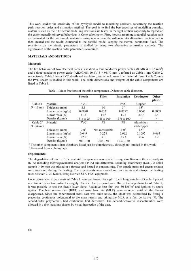
III/2 III/3

Modelling

Formulation

All the simulations were made using Fire Dynamics Simulator (FDS), version 5.5.2 [10]. In the model, the reaction rate of the pyrolysis reactions is calculated using Arrhenius equation

s

ijN

s

isijij RT

EAr

ijs

exp,

0

,

,(1)

where subscript i denotes the ith material component and j the jth reaction. ρs,i is the solid density of the component, and ρs,0 is the original density of the layer [10]. The solid phase heat conduction is solved in one dimension, according to the heat conduction equation

ss

ss

ss qxTk

xtTc

,(2)

where the chemical source term sq is

m rN

iijr

N

jijss Hxrxq

1,

10 )()( .

(3)

A mixture fraction based combustion model was used in the Cone calorimeter simulations.

Models of the Experiments

A simple model of the TGA experiment in Nitrogen atmosphere was created. The gas phase heat and mass transport were neglected in the model and the experiment was assumed to be 0-dimensional, in which case the dimensions of the simulation domain do not affect the results. The bottom of the domain was assigned with the sample material and the side walls and ceiling were heated according to the specified heating rate. As the TGA experiments were carried out for each component separately, the model included just one homogenous layer of material.

The Cone calorimeter model had dimensions of 30 30 40 cm3. The sample (10 10 cm2) was placed in the middle of the bottom boundary and all the other walls were open. The computational mesh wasextremely coarse (10 cm). A refinement of the mesh was not found to change the results significantly at an external heat flux of 50 kW/m2, but the computing time of the estimation process increased substantially. It is clear that a computation with such a coarse mesh cannot capture the details of the flame in the real Cone calorimeter experiment. However, it can provide an effective description of the flame heat flux to the sample surface because the combustion model burns most of the fuel within the one or two 10 cm cells above the sample, and because the source term of the gas phase radiation transport equation includes a specified fraction (usually 0.35) of the local heat release rate. The spark igniter was not included in the model because the ignition happens as soon as the fuel meets oxygen.

Cable 1 was modelled as a complete cable, neglecting the small amount of additional plastics. The approximation of Cable 1 structure as a planar surface is illustrated in Fig. 1. The first and third layersconsist of cable sheath material. The inner layer is a homogenous mixture of the insulation and filler materials. Conductors are not combustible and thus neglected in the model for simplicity and to save computational time in large scale simulations. According our previous simulations, the effect of the conductor on the model performance is not significant. The properties of the 2 cm thick backing layer were ρ = 800 kg/m3, ks = 0.1 W/m·K and cs = 1 kJ/kg·K. Cable 2 model included only one layer of sheath and the backing.

919

This work studies the sensitivity of the pyrolysis model to modelling decisions concerning the reaction path, reaction order and estimation method. The goal is to find the best practises of modelling complex materials such as PVC. Different modelling decisions are tested in the light of their capability to reproduce the experimentally observed behaviour in Cone calorimeter. First, models assuming a parallel reaction path are estimated for the two sample materials taking into account the softeners. An alternative reaction path is then created and the results compared to the parallel model keeping the thermal parameters fixed. The sensitivity on the kinetic parameters is studied by using two alternative estimation methods. The significance of the reaction order parameter is examined.

MATERIALS AND METHODS

Materials

The fire behaviour of two electrical cables is studied: a four conductor power cable (MCMK 4 × 1.5 mm2)and a three conductor power cable (AHXCMK 10 kV 3 × 95/70 mm2), referred as Cable 1 and Cable 2, respectively. Cable 1 has a PVC sheath and insulation, and an unknown filler material. From Cable 2, only the PVC sheath is studied in this work. The cable dimensions and weights of the cable components are listed in Table 1.

Table 1. Mass fractions of the cable components. D denotes cable diameter.

Sheath Filler Insulation Conductor Otherplastic

Cable 1D =13 mm

Material PVC - PVC Copper -Thickness (mm) 2.5 10 3b 15b -Linear mass (kg/m) 0.0898 0.0321 0.0297 0.0647 0.0009Linear mass (%) 41.3 14.8 13.7 29.7 0.4Density (kg/m3) 1316 25 1745 100 1375 100 - -

Cable 2a

D =54 mmMaterial PVC PE PE Aluminium

and copper-

Thickness (mm) 2.0b Not measurable 1.0b 1.5b -Linear mass (kg/m) 0.649 0.228 0.662 0.1097 0.063Linear mass (%) 22.8 8.0 23.3 38.6 2.2Density (kg/m3) 1500 30 950 50 1039 50 - -

a The other components than sheath are listed just for completeness, although not studied in this work. b Measured from a photograph.

Experimental

The degradation of each of the material components was studied using simultaneous thermal analysis (STA) including thermogravimetric analysis (TGA) and differential scanning calorimetry (DSC). A small sample (10 mg) was placed in a furnace and heated at constant rate. The sample mass and energy release were measured during the heating. The experiments were carried out both in air and nitrogen at heating rates between 2–20 K/min, using Netzsch STA 449C equipment.

Cone calorimeter experiments of Cable 1 were performed for eight 10 cm long samples of Cable 1 placed next to each other to construct a roughly 10 cm 10 cm exposed area. Due to the large diameter of Cable 2, it was possible to test the sheath layer alone. Radiative heat flux was 50 kW/m2 and ignition by spark igniter. The heat release rate (HRR) and mass loss rate (MLR) were recorded until all the flames disappeared. Since the experimental mass data was quite noisy, the MLR was determined by fitting apiecewise continuous polynomial to the mass results and taking the MLR as a first derivative [9]. The second-order polynomials had continuous first derivative. The second-derivative discontinuities were allowed in a few locations chosen by visual inspection of the data.

918

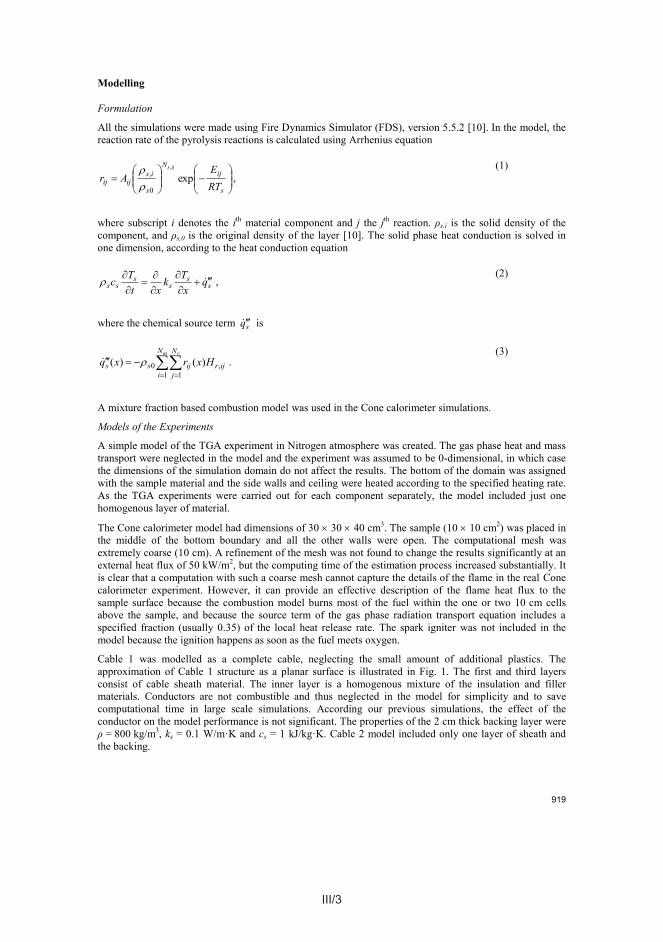
III/3

Modelling

Formulation

All the simulations were made using Fire Dynamics Simulator (FDS), version 5.5.2 [10]. In the model, the reaction rate of the pyrolysis reactions is calculated using Arrhenius equation

s

ijN

s

isijij RT

EAr

ijs

exp,

0

,

,(1)

where subscript i denotes the ith material component and j the jth reaction. ρs,i is the solid density of the component, and ρs,0 is the original density of the layer [10]. The solid phase heat conduction is solved in one dimension, according to the heat conduction equation

ss

ss

ss qxTk

xtTc

,(2)

where the chemical source term sq is

m rN

iijr

N

jijss Hxrxq

1,

10 )()( .

(3)

A mixture fraction based combustion model was used in the Cone calorimeter simulations.

Models of the Experiments

A simple model of the TGA experiment in Nitrogen atmosphere was created. The gas phase heat and mass transport were neglected in the model and the experiment was assumed to be 0-dimensional, in which case the dimensions of the simulation domain do not affect the results. The bottom of the domain was assigned with the sample material and the side walls and ceiling were heated according to the specified heating rate. As the TGA experiments were carried out for each component separately, the model included just one homogenous layer of material.

The Cone calorimeter model had dimensions of 30 30 40 cm3. The sample (10 10 cm2) was placed in the middle of the bottom boundary and all the other walls were open. The computational mesh wasextremely coarse (10 cm). A refinement of the mesh was not found to change the results significantly at an external heat flux of 50 kW/m2, but the computing time of the estimation process increased substantially. It is clear that a computation with such a coarse mesh cannot capture the details of the flame in the real Cone calorimeter experiment. However, it can provide an effective description of the flame heat flux to the sample surface because the combustion model burns most of the fuel within the one or two 10 cm cells above the sample, and because the source term of the gas phase radiation transport equation includes a specified fraction (usually 0.35) of the local heat release rate. The spark igniter was not included in the model because the ignition happens as soon as the fuel meets oxygen.

Cable 1 was modelled as a complete cable, neglecting the small amount of additional plastics. The approximation of Cable 1 structure as a planar surface is illustrated in Fig. 1. The first and third layersconsist of cable sheath material. The inner layer is a homogenous mixture of the insulation and filler materials. Conductors are not combustible and thus neglected in the model for simplicity and to save computational time in large scale simulations. According our previous simulations, the effect of the conductor on the model performance is not significant. The properties of the 2 cm thick backing layer were ρ = 800 kg/m3, ks = 0.1 W/m·K and cs = 1 kJ/kg·K. Cable 2 model included only one layer of sheath and the backing.

919

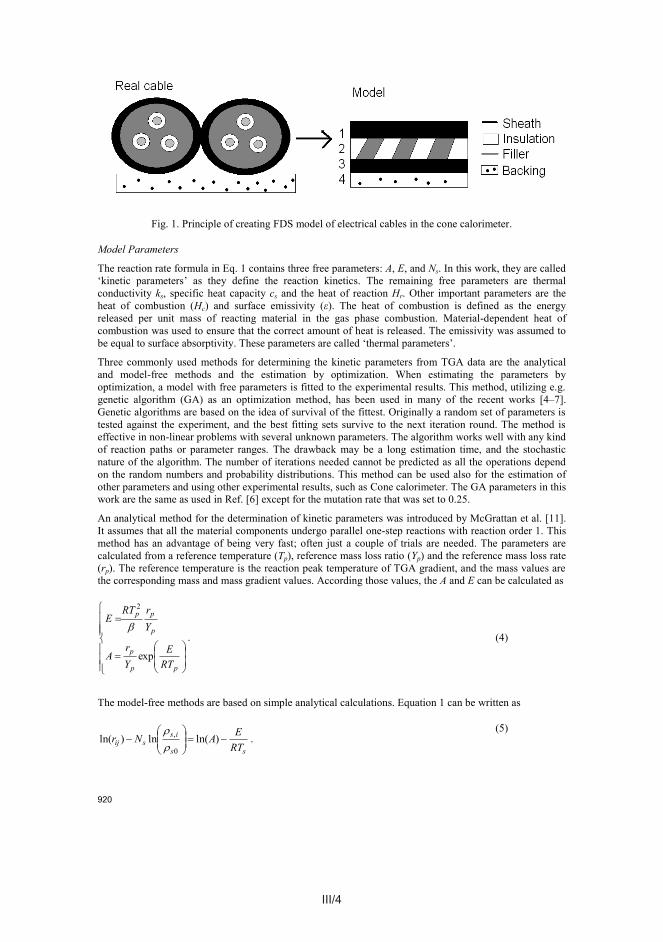
III/4 III/5

The reaction order Ns is a modelling choice. After choosing Ns, the unknown parameters, A and E can be determined by fitting a straight line to the plot of the left hand side against 1/Ts. This method is relatively fast and does not assume anything of the reaction order. However, it is quite sensitive for the choice of the temperature area considered and the details of the fitting process. Practical aspects of model-free methods were recently discussed by Kim [12].

Thermal parameters can be either directly measured or estimated from a Cone calorimeter test. Typical measured values are the specific heat capacity and the heat of reaction that can be obtained using DSC. The measurement of thermal conductivity is possible for building materials, for instance, but unpractical for small plastic samples, such as the components of electrical cables, or materials undergoing thermal degradation in the interesting temperature range. The effective heat of combustion, derived from the Cone calorimeter results, can sometimes be used as a material property if the relative proportions of the pyrolyzing materials are known over the time of the experiment. Alternatively, the heats of combustion can be estimated like the other thermal parameters by considering the difference between the measured and simulated effective heats of combustion as one of the measures of model fitness.

RESULTS AND DISCUSSION

Parallel Reactions - Model

The TGA results of the sheath materials of Cables 1 and 2 were found to be very close to each other.Therefore, the kinetic parameters were only estimated for Cable 1 and used for the sheaths of both cables. The sheath material was assumed to be a homogenous mixture of three independent components. A parallel reaction path with free reaction orders was used. A genetic algorithm was used for the estimation. The reaction path and the kinetic parameters are shown in Fig. 2 and the comparison of experimental and simulated TGA results in Fig. 3. The results fit slightly better for Cable 1, for which the parameters were estimated, but the difference to Cable 2 is not large. The reaction paths and kinetic parameters of the Cable 1 filler and insulation materials are shown in Figs. 4 and 5, respectively.

Fig. 2. Parallel model reaction path and kinetic parameters for the cable sheath. A in s-1 and E in kJ/kmol.

(a) (b)

Fig. 3. TGA results (10 K/min) for cable sheaths and FDS fit: (a) TGA; (b) Gradient of TGA.

921

Fig. 1. Principle of creating FDS model of electrical cables in the cone calorimeter.

Model Parameters

The reaction rate formula in Eq. 1 contains three free parameters: A, E, and Ns. In this work, they are called „kinetic parameters‟ as they define the reaction kinetics. The remaining free parameters are thermal conductivity ks, specific heat capacity cs and the heat of reaction Hr. Other important parameters are the heat of combustion (Hc) and surface emissivity (ε). The heat of combustion is defined as the energy released per unit mass of reacting material in the gas phase combustion. Material-dependent heat of combustion was used to ensure that the correct amount of heat is released. The emissivity was assumed to be equal to surface absorptivity. These parameters are called „thermal parameters‟.

Three commonly used methods for determining the kinetic parameters from TGA data are the analytical and model-free methods and the estimation by optimization. When estimating the parameters by optimization, a model with free parameters is fitted to the experimental results. This method, utilizing e.g. genetic algorithm (GA) as an optimization method, has been used in many of the recent works [4–7].Genetic algorithms are based on the idea of survival of the fittest. Originally a random set of parameters is tested against the experiment, and the best fitting sets survive to the next iteration round. The method is effective in non-linear problems with several unknown parameters. The algorithm works well with any kind of reaction paths or parameter ranges. The drawback may be a long estimation time, and the stochastic nature of the algorithm. The number of iterations needed cannot be predicted as all the operations depend on the random numbers and probability distributions. This method can be used also for the estimation of other parameters and using other experimental results, such as Cone calorimeter. The GA parameters in this work are the same as used in Ref. [6] except for the mutation rate that was set to 0.25.

An analytical method for the determination of kinetic parameters was introduced by McGrattan et al. [11]. It assumes that all the material components undergo parallel one-step reactions with reaction order 1. This method has an advantage of being very fast; often just a couple of trials are needed. The parameters are calculated from a reference temperature (Tp), reference mass loss ratio (Yp) and the reference mass loss rate (rp). The reference temperature is the reaction peak temperature of TGA gradient, and the mass values are the corresponding mass and mass gradient values. According those values, the A and E can be calculated as

pp

p

p

pp

RTE

Yr

A

YrRT

E

exp

2

. (4)

The model-free methods are based on simple analytical calculations. Equation 1 can be written as

ss

issij RT

EANr

)ln(ln)ln(

0

,

.(5)

920

III/5

The reaction order Ns is a modelling choice. After choosing Ns, the unknown parameters, A and E can be determined by fitting a straight line to the plot of the left hand side against 1/Ts. This method is relatively fast and does not assume anything of the reaction order. However, it is quite sensitive for the choice of the temperature area considered and the details of the fitting process. Practical aspects of model-free methods were recently discussed by Kim [12].

Thermal parameters can be either directly measured or estimated from a Cone calorimeter test. Typical measured values are the specific heat capacity and the heat of reaction that can be obtained using DSC. The measurement of thermal conductivity is possible for building materials, for instance, but unpractical for small plastic samples, such as the components of electrical cables, or materials undergoing thermal degradation in the interesting temperature range. The effective heat of combustion, derived from the Cone calorimeter results, can sometimes be used as a material property if the relative proportions of the pyrolyzing materials are known over the time of the experiment. Alternatively, the heats of combustion can be estimated like the other thermal parameters by considering the difference between the measured and simulated effective heats of combustion as one of the measures of model fitness.

RESULTS AND DISCUSSION

Parallel Reactions - Model

The TGA results of the sheath materials of Cables 1 and 2 were found to be very close to each other.Therefore, the kinetic parameters were only estimated for Cable 1 and used for the sheaths of both cables. The sheath material was assumed to be a homogenous mixture of three independent components. A parallel reaction path with free reaction orders was used. A genetic algorithm was used for the estimation. The reaction path and the kinetic parameters are shown in Fig. 2 and the comparison of experimental and simulated TGA results in Fig. 3. The results fit slightly better for Cable 1, for which the parameters were estimated, but the difference to Cable 2 is not large. The reaction paths and kinetic parameters of the Cable 1 filler and insulation materials are shown in Figs. 4 and 5, respectively.

Fig. 2. Parallel model reaction path and kinetic parameters for the cable sheath. A in s-1 and E in kJ/kmol.

(a) (b)

Fig. 3. TGA results (10 K/min) for cable sheaths and FDS fit: (a) TGA; (b) Gradient of TGA.

921

III/6 III/7

bounds of the corresponding estimation ranges. This means that the optimization algorithm could not find a good agreement within the estimation range, and it might be possible to obtain a better fitting model with a wider estimation range. It is interesting that even though the reaction paths and kinetic parameters were identical for the two cables, the thermal parameters resulting from the estimation process turned out be quite different. The most significant difference can be found for Hc of the first component of the sheath. For Cable 1, at 35 % fuel yield it is 40 MJ/kg while for Cable 2 with the same fuel yield only 15 MJ/kg.

(a) (b)

Fig. 7. Comparison of experimental and simulated Cone calorimeter results of sheath of Cable 2 at 50 kW/m2: (a) heat release rate; (b) mass loss rate.

Table 2. Thermal parameters of the cable models. „Sheath (N = 1)‟ of Cable 1 is related to the section Effect of the Kinetic Parameters. The emissivities for Components 1–3 are all 1.0.

Component 1 Component 2ks

(W/m·K)cs

(kJ/kg·K)Hr

(kJ/kg)Hc

(MJ/kg)ks

(W/m·K)cs

(kJ/kg·K)Hr

(kJ/kg)Hc

(MJ/kg)Cable 1Sheath (N free) 0.25 2.0 800 40 0.15 2.8 700 45Sheath (N = 1) 0.14 3.5 1110 45 0.1a 0.8 1760 45b

Insulation 0.77 3.3 450 - 0.4 2.5 300 45b

Filler 0.65 2.5 800 30 0.45 0.81 300 40Cable 2Sheath 0.1a 1.5 1630 15 0.26 1.6 740 23.9

Component 3 Residueks

(W/m·K)cs

(kJ/kg·K)Hr

(kJ/kg)Hc

(MJ/kg)ks

(W/m·K)cs

(kJ/kg·K)

Cable 1Sheath (N free) 0.15 2.09 700 40b 0.9 2.0 1.0Sheath (N = 1) 0.42 0.8 950 45b 0.8b 2.0 0.99Insulation 0.79 0.8 300 40 0.67 1.3 1.0Filler - - - - 0.25 1.3 1.0Cable 2Sheath 0.21 1.37 1860 27.8 0.79 2.0 0.98a At lower bound of estimation range. b At upper bound of estimation range.

923

Fig. 4. Reaction path and kinetic parameters for the insulating material. A in s-1 and E in kJ/kmol.

Fig. 5. Reaction path and kinetic parameters for the filler. A in s-1 and E in kJ/kmol.

(a) (b)

Fig. 6. Comparison of experimental and simulated Cone calorimeter results of Cable 1 at 50 kW/m2: (a) heat release rate; (b) mass loss rate.

The thermal parameters were estimated from the Cone calorimeter experiments. The emissivities of the initial material components were set to 1.0, but non-unity emissivities were allowed for the chars. This choice was made because earlier sensitivity studies had shown that the results are sensitive to the emissivity of char but not to the emissivity of the virgin material. Besides, the virgin emissivity only plays a role during the short time before the ignition. As the conductivities and the specific heats were treated as constants over temperature, the estimated values must be treated as averages over corresponding temperature ranges. The middle layer of Cable 1 is a mixture of 48.1 % insulator and 51.9 % filler. The layer thicknesses from first to last are 2.73 mm, 3.2 mm and 2.73 mm. A comparison of simulated and measured HRR and MLR is shown in Fig. 6. The model predicts very accurately both the ignition time and shapes of the two peaks in the curves. Including data for different radiation levels would probably reduce the model fitness into a single curve but improve the parameter generality. Inclusion of surface temperature measurement, as in [7], would add another dimension to the fitness assessment. However, performing such measurements for thermoplastic samples with complex structure may be challenging.

For Cable 2, only the sheath layer (2.9 mm thick) was modelled. A comparison of the experimental and model HRR and MLR is shown in Fig. 7. Again, ignition time is accurately predicted and the overall shapes of the curves are satisfactory, although not as accurate as for Cable 1. The thermal parameters are listed in Table 2. Some of the conductivity and heat of combustion values are equal to the lower or upper

922

III/7

bounds of the corresponding estimation ranges. This means that the optimization algorithm could not find a good agreement within the estimation range, and it might be possible to obtain a better fitting model with a wider estimation range. It is interesting that even though the reaction paths and kinetic parameters were identical for the two cables, the thermal parameters resulting from the estimation process turned out be quite different. The most significant difference can be found for Hc of the first component of the sheath. For Cable 1, at 35 % fuel yield it is 40 MJ/kg while for Cable 2 with the same fuel yield only 15 MJ/kg.

(a) (b)

Fig. 7. Comparison of experimental and simulated Cone calorimeter results of sheath of Cable 2 at 50 kW/m2: (a) heat release rate; (b) mass loss rate.

Table 2. Thermal parameters of the cable models. „Sheath (N = 1)‟ of Cable 1 is related to the section Effect of the Kinetic Parameters. The emissivities for Components 1–3 are all 1.0.

Component 1 Component 2ks

(W/m·K)cs

(kJ/kg·K)Hr

(kJ/kg)Hc

(MJ/kg)ks

(W/m·K)cs

(kJ/kg·K)Hr

(kJ/kg)Hc

(MJ/kg)Cable 1Sheath (N free) 0.25 2.0 800 40 0.15 2.8 700 45Sheath (N = 1) 0.14 3.5 1110 45 0.1a 0.8 1760 45b

Insulation 0.77 3.3 450 - 0.4 2.5 300 45b

Filler 0.65 2.5 800 30 0.45 0.81 300 40Cable 2Sheath 0.1a 1.5 1630 15 0.26 1.6 740 23.9

Component 3 Residueks

(W/m·K)cs

(kJ/kg·K)Hr

(kJ/kg)Hc

(MJ/kg)ks

(W/m·K)cs

(kJ/kg·K)

Cable 1Sheath (N free) 0.15 2.09 700 40b 0.9 2.0 1.0Sheath (N = 1) 0.42 0.8 950 45b 0.8b 2.0 0.99Insulation 0.79 0.8 300 40 0.67 1.3 1.0Filler - - - - 0.25 1.3 1.0Cable 2Sheath 0.21 1.37 1860 27.8 0.79 2.0 0.98a At lower bound of estimation range. b At upper bound of estimation range.

923

III/8 III/9

(a) (b)

(c) (d)

(e) (f)

Fig. 9. Sensitivity of the cable pyrolysis for the reaction path in TGA (a and b) and cone calorimeter (c–f):(c) HRR of Cable 1; (d) MLR of Cable 1; (e) HRR of Cable 2 sheath; (f) MLR of Cable 2 sheath.

925

Fig. 8. Consecutive model reaction path and kinetic parameters for the cable sheath; (a) at lower bound of the estimation range; (b) at upper bound of estimation range.

Effect of the Reaction Scheme

The parallel model the reaction path describing the sheath pyrolysis consists of three parallel reactions, which is the simplest possible model being able to reproduce the three distinct reactions observed in the TGA curve. In the absence of information about the true chemical formulations and reactions, which is often the case in fire modelling, the reaction path is modeller's choice. The only evidence for or against the chosen scheme comes from the fitting process. Alternative schemes, such as a consecutive reaction path, must be evaluated based on their fitting capability and the credibility of the best-fitting model parameters. A consecutive reaction path was therefore applied to the sheath reactions, yielding the kinetic parameters shown in Fig. 8. The estimated values for the pre-exponential factors of components 2 and 3 correspond to the upper and lower bounds of the estimation range, indicating that the algorithm could not find satisfactory fit in the range of these parameters. For better agreement with consecutive reactions, the range of these parameters should be extended. A comparison of the parallel and consecutive model predictions of TGA at 10 K/min heating rate is shown in Figs. 9a–b. Both reaction paths can accurately predict the experimental results. The other model parameters were the same for both models, as listed in Table 2. The effect of the reaction path on the simulated cone calorimeter results is shown in Figs. 9c–f. Even though the TGA curves are quite close to each other, the cone calorimeter results differ significantly. In the consecutive reaction path, the third reaction is limited by the second one. Parallel reaction path does not have this limitation and this could explain the differences in the cone calorimeter results. For Cable 1, the consecutive reaction scheme yields lower heat release and mass loss rates and longer extinction times than the parallel scheme.The differences are in the same direction but less significant for the sheath of Cable 2.

In theory, the degradation of rigid PVC could be modelled as a two-stage process: the first releasing HCl and the second producing combustible fuel vapour and residue. Flexible PVC contains softeners, such as phthalates, with degradation products such as benzene, naphthalene and anthracene that may be combustible and must be considered in the pyrolysis modelling. In the presence of Oxygen and heat these compounds can burn, having a heat of combustion over 40 MJ/kg [13]. In the pyrolysis modelling, the release of combustible products is considered by specifying a non-zero fuel yield for the first reaction of PVC. In the most accurate model for the cable sheaths, the fuel yield of the first reaction was 35 %. The effect of this parameter for the HRR prediction is demonstrated in Fig. 10 showing the HRR results for both cables at three different fuel yields 0 %, 15 % and 35 % of the first reaction step. The smaller-than-optimal yield of fuel can, to some extent, be compensated by adjusting the heat of combustion of the corresponding material. The values should however be chosen from a reasonable range, i.e. smaller or equal to 50 MJ/kg.

In the parallel model, both solid components produce independently fuel and char. One could also choose the mass fractions so that only the second solid reaction produces char, and the other one fuel. The cone calorimeter results are not sensitive to this choice for any of the cable models.

924

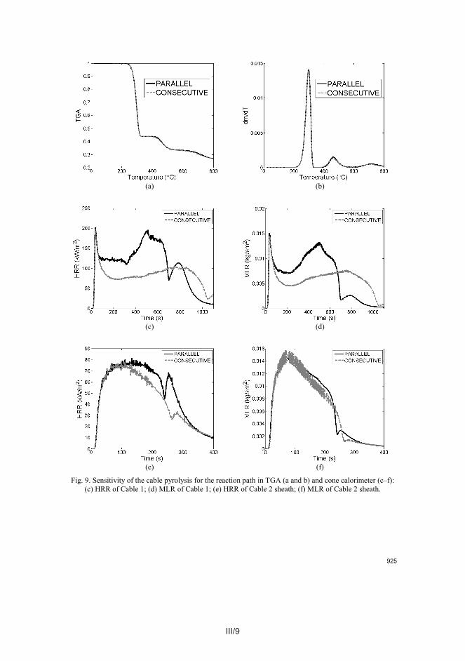
III/9

(a) (b)

(c) (d)

(e) (f)

Fig. 9. Sensitivity of the cable pyrolysis for the reaction path in TGA (a and b) and cone calorimeter (c–f):(c) HRR of Cable 1; (d) MLR of Cable 1; (e) HRR of Cable 2 sheath; (f) MLR of Cable 2 sheath.

925

III/10 III/11

(a) (b)

(c) (d)

Fig. 11. Sensitivity of the simulation results to different sets of parameters for Cable 1: (a) TGA at 10 K/min; (b) gradient of TGA at 10 K/min; (c) HRR at 50 kW/m2; (d) MLR at 50 kW/m2.

The reaction order affects the sharpness of the TGA curve. In Fig. 12, models with two different reaction orders are compared. For „N free‟, the kinetic parameters were those shown in Fig. 2 and for „N = 1‟, the parameters estimated by GA, shown in Table 3 were used. Thermal parameters were the same in both models (Table 2). TGA curves (Fig. 12a–b) are very close to each other, but the cone results (Fig. 12c–d) show more differences. Both heat release and mass loss rates are higher when Ns is freely chosen. The magnitude of the differences is somewhat surprising, considering the very close match in TGA. The „N = 1‟model gives lower HRR than the version with free N, even though the heat of combustion and all the other thermal parameters are the same. The explanation can be found in the different sources of fuel in these two models, as indicated by Fig. 2 and Table 3. The total fuel yields are the same for the two models (otherwise TGA curves would be different) but the heats of combustion of the components 2 and 3 are different (45 and 40 MJ/kg, respectively, Table 2).

927

(a) (b)

Fig. 10. Effect of first reaction fuel yield at 50 K/min: (a) Cable 1; (b) Cable 2 sheath.

Effect of the Kinetic Parameters

Due to the so-called „compensation effect‟, the values of A and E are usually not important just by themselves, but their ratio is significant [14]. Many different sets of kinetic parameters can thus produce equally accurate prediction for TGA results. Two different sets of kinetic parameters were estimated with constraint Ns = 1. One was estimated using the genetic algorithm (GA) and another one using the analytical method. The reaction paths were parallel and the differences were only allowed in the kinetic parameters and fuel allocation of the components. The results are shown in Fig. 11 and kinetic parameters listed in Table 3. The TGA predictions are quite similar with the two sets of parameters. Using the thermal parameters listed in Table 2, the cone calorimeter results do not show any significant difference either, indicating that there is no preference over one of the estimation methods. Due to the use of a non-optimized set of thermal parameters, neither of the results shown in Figs. 11c–d are close to the experimental result, though. Both estimation methods have their advantages. The GA takes a longer time than the analyticalmethod, but is more flexible for the changes in the reaction path and the reaction order. The analytical method provides fast results, but the model has to be limited to parallel reaction path with reaction order 1.

A comparison between Table 3 and Fig. 2 shows that the mass allocations between components 2 and 3 have been exchanged. The integrated mass loss and heat release are still quite close to each other due to the different fuel yields. This peculiarity is caused by the nature of the parallel reaction scheme, for which the assignment of reactions between the reactions observed in TGA by the stochastic optimization cannot be pre-determined, if the parameter ranges are wide enough. This should be kept in mind when interpreting the results of the stochastic optimization methods.

Table 3. Kinetic parameters with Ns = 1.

A (s-1) E (kJ/kmol) Residue yieldMethod: GAComponent 1 (56 %) 1.08 × 1015 1.85 × 105 0 %Component 2 (11 %) 5.93 × 1011 1.99 × 105 6 %Component 3 (33 %) 1.08 × 1012 2.73 × 105 83 %Method: AnalyticalComponent 1 (56 %) 9.80 × 1018 2.24 × 105 0 %Component 2 (10 %) 3.40 × 1036 5.40 × 105 0 %Component 3 (34 %) 1.67 × 109 2.21 × 105 79 %

926

III/11

(a) (b)

(c) (d)

Fig. 11. Sensitivity of the simulation results to different sets of parameters for Cable 1: (a) TGA at 10 K/min; (b) gradient of TGA at 10 K/min; (c) HRR at 50 kW/m2; (d) MLR at 50 kW/m2.

The reaction order affects the sharpness of the TGA curve. In Fig. 12, models with two different reaction orders are compared. For „N free‟, the kinetic parameters were those shown in Fig. 2 and for „N = 1‟, the parameters estimated by GA, shown in Table 3 were used. Thermal parameters were the same in both models (Table 2). TGA curves (Fig. 12a–b) are very close to each other, but the cone results (Fig. 12c–d) show more differences. Both heat release and mass loss rates are higher when Ns is freely chosen. The magnitude of the differences is somewhat surprising, considering the very close match in TGA. The „N = 1‟model gives lower HRR than the version with free N, even though the heat of combustion and all the other thermal parameters are the same. The explanation can be found in the different sources of fuel in these two models, as indicated by Fig. 2 and Table 3. The total fuel yields are the same for the two models (otherwise TGA curves would be different) but the heats of combustion of the components 2 and 3 are different (45 and 40 MJ/kg, respectively, Table 2).

927

III/12 III/13

Fig. 13. Cone calorimeter results at 50 kW/m2 with separately estimated thermal parameters for the two sets of kinetic parameters: (a) heat release rate; (b) mass loss rate.

CONCLUSIONS

The effects of the modelling decisions and methods on the pyrolysis modelling of two PVC cables were studied. The kinetic and thermal parameters were estimated from the TGA and cone calorimeter experiments. The TGA results of the cable sheaths were so close to each other that the same kinetic parameters were used for both cables. With three structural components describing the structure of the complete cable (sheath, insulation and filler) and two to three material components for each structural components, the estimation algorithm was able to find a set of parameters that accurately reproduced the mass loss and heat release rate curves at one radiation level.

The effect of the reaction path was studied by comparing the results obtained with parallel and consecutive reaction schemes. The effect on the TGA results was shown to be very small. However, a substantial effect was observed in the cone calorimeter results, where the consecutive scheme produced significantly lower heat release and mass loss rates. The plasticizers that are used in the production of flexible PVC were found to have a strong effect on the early part of the HRR curves. These additives can make up 30–40 wt. % of the flexible PVC, and should therefore be taken into account in the pyrolysis model as a non-zero fuel yield for the first degradation reaction. The exact allocation of the fuel between the components was found to be unimportant, as long as the correct yields of fuel and residue were retained.

When first-order reactions were assumed and two sets of parameters estimated, no significant differences were found. Both estimation methods accurately reproduced the TGA curve. The different values of reaction order made more difference. The TGA predictions were almost equal, but the heat release and mass loss were greatly reduced when the reaction order was forced to one without estimating a separate set of thermal parameters. When the separate thermal parameters were estimated for the two different sets of kinetic parameters, equally good fits to the experimental data were again achieved, but the estimated values of the thermal parameters were very different.

The reaction path, estimation method and the parameter sets can be chosen in many ways when estimating the pyrolysis model parameters from the cone calorimeter results. Thermal parameters can, to some extent, compensate the choices made for the kinetic model. Nothing implies that one way to make the choice would be better than another. This is a topic that requires more research and discussion. However, the results demonstrate that the thermal parameters estimated for one kinetic model should not be used for another, unless the difference between the kinetic models considers only fuel yields or different pairs of Aand E with same Ns. It is very important to check the model behaviour when changing the model details or the simulation code version. Also, the universality of the thermal parameters could be improved by considering a wider set of experimental data during the parameter estimation process, such as sample temperatures, different heat flux levels and different atmospheres.

929

(a) (b)

(c) (d)

Fig. 12. Comparison of results with different reaction orders for Cable 1: (a) TGA at 10 K/min; (b) gradient of TGA at 10 K/min; (c) heat release rate at 50 kW/m2; (d) mass loss rate at 50 kW/m2.

The relatively strong effect that the kinetic parameters have on the cone calorimeter simulation can be „compensated‟ by adjusting other parameters. When the thermal parameters for sheath were estimated separately for the both kinetic schemes, „N free‟ and „N = 1‟, the HRR and MLR predictions (Fig. 13) come very close to each other and closer to the experimental curve. The parameter values, in turn, are significantly different. They are listed in Table 2 as „Cable 1 Sheath (N = 1)‟. The greatest differences are found in the specific heat capacities of the initially existing material components (i.e. not residue), the heat of reaction of the second component and the thermal conductivity of the third component.

From a theoretical viewpoint, it may be discomforting to see that the thermal parameters can „compensate‟for the choices concerning the reaction scheme or the values of the kinetic coefficients. This problem should be examined from the viewpoint of the experimental and model uncertainty: If one wants to test the capability of a model to explain observed experimental evidence, one must also take into account the uncertainty associated with the experimental data and conditions, and the model input parameters. If the model can or cannot be fit to the test data within the given uncertainty bounds of the thermal parameters, that is all we can say. Of course, if one can directly measure any of the parameters with a sufficient accuracy, the size of the parameter space would be reduced, and the weight of the given scenario increased as an evidence of the model validity. Direct measurements of the properties are therefore highly recommended whenever possible.

928

III/13

Fig. 13. Cone calorimeter results at 50 kW/m2 with separately estimated thermal parameters for the two sets of kinetic parameters: (a) heat release rate; (b) mass loss rate.

CONCLUSIONS

The effects of the modelling decisions and methods on the pyrolysis modelling of two PVC cables were studied. The kinetic and thermal parameters were estimated from the TGA and cone calorimeter experiments. The TGA results of the cable sheaths were so close to each other that the same kinetic parameters were used for both cables. With three structural components describing the structure of the complete cable (sheath, insulation and filler) and two to three material components for each structural components, the estimation algorithm was able to find a set of parameters that accurately reproduced the mass loss and heat release rate curves at one radiation level.

The effect of the reaction path was studied by comparing the results obtained with parallel and consecutive reaction schemes. The effect on the TGA results was shown to be very small. However, a substantial effect was observed in the cone calorimeter results, where the consecutive scheme produced significantly lower heat release and mass loss rates. The plasticizers that are used in the production of flexible PVC were found to have a strong effect on the early part of the HRR curves. These additives can make up 30–40 wt. % of the flexible PVC, and should therefore be taken into account in the pyrolysis model as a non-zero fuel yield for the first degradation reaction. The exact allocation of the fuel between the components was found to be unimportant, as long as the correct yields of fuel and residue were retained.

When first-order reactions were assumed and two sets of parameters estimated, no significant differences were found. Both estimation methods accurately reproduced the TGA curve. The different values of reaction order made more difference. The TGA predictions were almost equal, but the heat release and mass loss were greatly reduced when the reaction order was forced to one without estimating a separate set of thermal parameters. When the separate thermal parameters were estimated for the two different sets of kinetic parameters, equally good fits to the experimental data were again achieved, but the estimated values of the thermal parameters were very different.

The reaction path, estimation method and the parameter sets can be chosen in many ways when estimating the pyrolysis model parameters from the cone calorimeter results. Thermal parameters can, to some extent, compensate the choices made for the kinetic model. Nothing implies that one way to make the choice would be better than another. This is a topic that requires more research and discussion. However, the results demonstrate that the thermal parameters estimated for one kinetic model should not be used for another, unless the difference between the kinetic models considers only fuel yields or different pairs of Aand E with same Ns. It is very important to check the model behaviour when changing the model details or the simulation code version. Also, the universality of the thermal parameters could be improved by considering a wider set of experimental data during the parameter estimation process, such as sample temperatures, different heat flux levels and different atmospheres.

929

III/14 1

ACKNOWLEDGEMENTS

This work has been partially funded by the State Nuclear Waste Management Fund (VYR). Authors would like to thank Tuula Leskelä from Aalto University School of Science and Technology for the thermogravimetric experiments, and Konsta Taimisalo and Johan Mangs from VTT for help when conducting cone calorimeter experiments.

REFERENCES

[1] DeLassus, P.T., and Whiteman, N.F., “Physical and Mechanical Properties of Some Important Polymers,” Polymer Handbook (4th ed.), Brandrup, J., Immergut, E.,H. Grulke, E.A., Abe, A., Bloch, D.R. (ed. ) Wiley, New York, 1999, pp. 159-169.

[2] Papazoglou, E., Flame Retardants for Plastics. Handbook of building materials for fire protection, Harper, C.A. (ed.), McGraw-Hill, New York, NY, 2004. pp. 4.1-4.88.

[3] Marcilla, A., and Beltrán, M., (1995) Thermogravimetric kinetic study of poly(vinyl Chloride) pyrolysis. Polymer Degradation and Stability 48: 219-229. http://dx.doi.org/10.1016/0141-3910(95)00050-V

[4] Lautenberger, C., Rein, G., and Fernandez-Pello, C., (2006). The application of a genetic algorithm to estimate material properties for fire modeling from bench-scale fire test data. Fire Safety Journal 41: 204-214. http://dx.doi.org/10.1016/j.firesaf.2005.12.004

[5] Rein, G., Lautenberger, C., Fernandez-Pello, C., Torero, J., and Urban, D., (2006). Application of genetic algorithms and thermogravimetry to determine the kinetics of polyurethane foam in smoldering combustion. Combustion and Flame 146: 95-108. http://dx.doi.org/10.1016/j.combustflame.2006.04.013

[6] Matala, A., Hostikka, S. and Mangs, J., 2009. Estimation of Pyrolysis Model Parameters for Solid Materials Using Thermogravimetric Data. Fire Safety Science 9: 1213-1223. http://dx.doi.org/10.3801/IAFSS.FSS.9-1213

[7] Lautenberger, C., and Fernandez-Pello, C., (2009) Generalized pyrolysis model for combustible solids. Fire Safety Journal 44: 819-839. http://dx.doi.org/10.1016/j.firesaf.2009.03.011

[8] Chaos, M., Khan, M.M., Krishnamoorthy, N., de Ris, J.L., and Dorofeev, S.B., “Evaluation of optimization schemes and determination of solid fuel properties for CFD fire models using bench-scale pyrolysis tests,” Proceedings of the Combustion Institute 33 (2), 2011, pp. 2599-2606.http://dx.doi.org/10.1016/j.proci.2010.07.018

[9] Baroudi, D., 1993. “Piecewise least squares fitting technique using finite interval method with Hermite polynomials,” VTT Technical Research Centre of Finland, VTT Publications 135, Espoo, Finland. 27 p.

[10] McGrattan, K., Hostikka, S., Floyd, J., Baum, H., Rehm, R., Mell, W., and McDermott, R., “Fire Dynamics Simulator (Version 5) Technical Reference Guide. Volume 1: Mathematical Model,”NIST Special Publication 1018-5. Gaithersburg, MD, 2010.

[11] McGrattan, K., McDermott, R., Mell, W., Forney, G., Floyd, J., Hostikka, S., and Matala, A. “Modeling the burning of complicated objects using Lagrangian particles,” Proceedings of the Twelfth International Interflam Conference, 2010, pp. 743-753.

[12] Kim, E., Shivkumar, S., and Dembsey, N., “Thermal degradation kinetics modeling for pyrolysis modeling using fire retarded thermoset polymer resins,” Proceedings of the Twelfth International Interflam Conference. 2010, pp. 475-486.

[13] Appendix C. DiNenno, P.J. (ed.) SFPE Handbook of Fire Protection Engineering (4th ed.), National Fire Protection Association, Quincy, MA 02269, 2008.

[14] Nikolaev, A.V., Gorbatchev, V.M. and Logvinenko, V.A. (1974) Special features of the compensation effect in non-isothermal kinetics of solid-phase reactions, Journal of Thermal Analysis 6: 473-477. http://dx.doi.org/10.1007/BF01914927

930

1

PUBLICATION IV

Modelling polymeric material using Microscale combustion

calorimetry and other small scale data

Manuscript, submitted to Fire and Materials

in June 2013.

IV/1

M O D E L L I N G P O L Y M E R I C M A T E R I A L U S I N G M I C R O S C A L E C O M B U S T I O N C A L O R I M E T R Y A N D O T H E R S M A L L S C A L E

D A T A

Anna Matala and Simo Hostikka VTT Technical Research Centre of Finland

P.O. Box 1000, FI-02044 VTT [email protected]

Keywords: pyrolysis modelling, Microscale combustion calorimetry, cables, PVC Abstract

A challenge encountered by many practicing fire engineer carrying out fire modelling is that the combustible fuel is not completely well-known. Practical materials may, for instance, be identified as some well-known polymer, but this is usually not the whole truth from the viewpoint of the fire behaviour. Besides of the nominal polymer, the blend may include large quantities of different additives that affect the thermal degradation and combustion of the material. Until now, the effect of these additives has been taken into account in the modelling by adjusting the thermal parameters when fitting the model to the cone calorimeter results. Such a model captures the joint effect of all the components, but cannot distinguish between the combustible volatiles from additives and main polymer, which may lead to inaccurate prediction if the conditions, such as the heating rate, are significantly different. In this work we use Microscale Combustion Calorimetry for building a more accurate model of the polymer pyrolysis by combining the heat release rate measurements with the mass loss rate measured in Thermogravimetric Analysis. Two methods are developed and tested using a generic sample and a real PVC sheath of an electric cable. The results show that the methods are able to calculate the heat release rate correctly for the tested materials, and also estimating the sample composition to some extent.

Symbols

A Pre-exponential factor (s-1) Greek cp Specific heat capacity (kJ/kg/K) α Conversion E Activation energy (kJ/mol) β Heating rate (K/s) ΔH Heat of reaction (kJ/kg) ε Emissivity ΔHc Heat of combustion (kJ/kg) ρ Density (kg/m3) k Thermal conductivity (W/m/K) m Mass (kg) Subscripts m Mass loss rate (kg/s) 0 Initial nc Number of components eff Effective value nO2 Reaction order of oxidation F Fuel gas np Number of (gaseous) products. i Reaction index nr Number of reactions I Inert gas N Reaction order j Component index Qc Heat release (kJ) Z Residue

cQ Heat release rate (kW) Q/m0 Total heat release in MCC (MJ/kg) Z Residue yield (of total mass) T Temperature (K)

IV/2 IV/3

METHODS

Experimental methods

TGA is the most common small scale experiment for determining the reaction kinetics of the pyrolysis reaction. In TGA, a small sample (5-10 mg) is placed into a furnace that has either air or nitrogen atmosphere. The furnace is heated linearly at relatively slow heating rate, typically at 1-30 K/min. The small sample and slow heating rate ensure that the sample is in thermal equilibrium with the furnace. The mass of the sample is measured during the heating, and the experiment results the mass loss as a function of temperature. [6]

MCC, also known as Pyrolysis-combustion flow calorimetry, was developed at FAA in the beginning of the millennium [4],[5]. A small sample (5-10 mg) is placed into a pyrolyzer that operates similarly to TGA under either inert of oxidative ambient. The heating rates are higher than typically in TGA experiment, usually 1 K/s. The pyrolysis gases are then led to a combustor that has high temperature (up to 1000 °C) and sufficient oxygen ambient. The gases are completely combusted in few seconds, and the result is the heat release rate (often scaled with the sample mass) as a function of temperature.

Cone Calorimeter is the most commonly used bench scale experiment in fire research. A 10 x 10 cm2 sample is placed under a cone heater that directs a heat flux of 35-75 kW/m2 to the sample surface. The sample is ignited using an electric spark. During the experiment, mass and heat release rates are measured. [7]

Combining TGA and MCC results

MCC measures the heat release rate scaled by the initial mass of the sample. For complete burning at heat of combustion ΔHc and fuel yield yi,F, the result can be expressed as

icFiicFiic Hy

mmH

mm

mQ

,,0

,0

,

0

,

, (1)

where mF corresponds to the mass loss that is responsible of the heat release (the production of the fuel gas). The total heat release of the reaction i (when temperature range of the reaction is Ti-1 - Ti) can be written

i

i

i

i

t

ticFi

t

t

cic dtmmHydt

mQ

mQ

11 0,,

00

, . (2)

The material is considered to be composed of j pseudo-components that each degrades in one or more reactions yielding potentially fuel gas (combustible), inert gas (e.g. water vapour) and residue. The yields of the products are denotes as yijF, yijI and yijZ, respectively. Naturally a component may yield several different fuel gases during one reaction, but in the accuracy of the model only the

gross effect is significant. The total conversion (0

1mm

) of the reaction is

jijIj

ijFii

t

ti xyy

mmmdt

mmi

ti

)(0

1

0

, (3)

where xi is the mass fraction of the component j. The overall fuel yield of the reaction is therefore

ΔT Temperature range XO2 Oxygen volume fraction y yield Y Mass fraction

INTRODUCTION

Polymeric materials often include large amount of additives besides of the nominal polymer. The electrical cables, for instance, contain significant mass fractions of plasticizers, stabilizers and fillers. These additives are not reported by the manufacturer, and their concentrations are business secrets. This is a challenge commonly encountered by practicing fire engineer carrying out fire modelling. The problem is most pronounced in situations where the composition of the combustibles is not known at all, such as the fire investigation. The same problem is also faced when modelling industrial fires where the fuel may be formally known. The actual contents of the commercial material may be a very complicated blend of polymers and additives, as illustrated above for the electrical cables. A full chemical analysis of the combustible fuels could be used to reveal the contents of the fuels, at least qualitatively, but carrying out such an analysis would be impractical for many reasons. Simple and robust methods are therefore needed to determine the relevant pieces of information to support the fire modelling.

In this work, we use electrical cables as an example of material to be modelled. The additives of the cable components (e.g. phthalates, a plasticizer) are often combustible and may have other joint effects on the polymer degradation as well. In the pyrolysis modelling of the cable materials, these additives are usually taken into account simply by fitting the model to the experimental data [1]-[3]. The cone calorimeter has been until now the most commonly used experimental method that measures the heat release rate. The problem in cone calorimeter scale is that it only provides information about the effective heat of combustion, the joint effect of all the components degrading simultaneously. It does not provide information about the degradation temperatures or separate the heat release by reactions or components, which make the distinguishing between the components challenging.

Microscale Combustion Calorimetry (MCC) is a relatively new, experimental small scale device that was developed at Federal Aviation Administration (FAA) [4],[5]. It provides information about the heat release as a function of temperature, similarly to Thermogravimetric Analysis (TGA). By combining the information about mass loss and the simultaneous heat release, the heat of combustions of each reaction can be determined. Moreover, this information can be used in estimation of the sample composition and mass fractions.

In this work, the heat release rate measured by MCC is combined with mass loss measured by Thermogravimetric Analysis (TGA) at each reaction step. Two alternative methods are presented for building a reaction path using these results. The first one is a general model, which does not require any knowledge of the actual polymeric mixture. The second method is targeted for building a more complete and accurate model, and requires information about typical additives and their thermal degradation and heat of combustion. The results of both methods help to allocate the sample heat release to correct temperatures. Additionally, the second method can be used to estimate the mass fractions of main components in a polymer blend. These methods are applied to a generic sample in order to verify and validate the methods, and to a real PVC sheath of an electric cable. The results are compared in small and bench scale using experimental data and numerical simulations. The effect of surface oxidation is also taken into account in the cone calorimeter simulations.

IV/3

METHODS

Experimental methods

TGA is the most common small scale experiment for determining the reaction kinetics of the pyrolysis reaction. In TGA, a small sample (5-10 mg) is placed into a furnace that has either air or nitrogen atmosphere. The furnace is heated linearly at relatively slow heating rate, typically at 1-30 K/min. The small sample and slow heating rate ensure that the sample is in thermal equilibrium with the furnace. The mass of the sample is measured during the heating, and the experiment results the mass loss as a function of temperature. [6]

MCC, also known as Pyrolysis-combustion flow calorimetry, was developed at FAA in the beginning of the millennium [4],[5]. A small sample (5-10 mg) is placed into a pyrolyzer that operates similarly to TGA under either inert of oxidative ambient. The heating rates are higher than typically in TGA experiment, usually 1 K/s. The pyrolysis gases are then led to a combustor that has high temperature (up to 1000 °C) and sufficient oxygen ambient. The gases are completely combusted in few seconds, and the result is the heat release rate (often scaled with the sample mass) as a function of temperature.

Cone Calorimeter is the most commonly used bench scale experiment in fire research. A 10 x 10 cm2 sample is placed under a cone heater that directs a heat flux of 35-75 kW/m2 to the sample surface. The sample is ignited using an electric spark. During the experiment, mass and heat release rates are measured. [7]

Combining TGA and MCC results

MCC measures the heat release rate scaled by the initial mass of the sample. For complete burning at heat of combustion ΔHc and fuel yield yi,F, the result can be expressed as

icFiicFiic Hy

mmH

mm

mQ

,,0

,0

,

0

,

, (1)

where mF corresponds to the mass loss that is responsible of the heat release (the production of the fuel gas). The total heat release of the reaction i (when temperature range of the reaction is Ti-1 - Ti) can be written

i

i

i

i

t

ticFi

t

t

cic dtmmHydt

mQ

mQ

11 0,,

00

, . (2)

The material is considered to be composed of j pseudo-components that each degrades in one or more reactions yielding potentially fuel gas (combustible), inert gas (e.g. water vapour) and residue. The yields of the products are denotes as yijF, yijI and yijZ, respectively. Naturally a component may yield several different fuel gases during one reaction, but in the accuracy of the model only the

gross effect is significant. The total conversion (0

1mm

) of the reaction is

jijIj

ijFii

t

ti xyy

mmmdt

mmi

ti

)(0

1

0

, (3)

where xi is the mass fraction of the component j. The overall fuel yield of the reaction is therefore

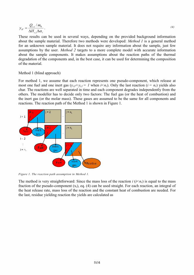
IV/4 IV/5

1

1

1

1

0,

1

1

0,

11

11

)/(1

11

)/(

rrrr

r

r

r

r

r

r

r

r

n

ii

InFnZn

n

ii

nc

ncIn

n

ii

nc

ncFn

Zyyy

ZH

mQy

ZH

mQy

. (5)

Method 2 (advanced approach)

For method 2, an initial evaluation of the material composition has to be made. This method tries to follow the real reaction paths of the main components as accurately as possible while avoiding unnecessary complex model. The main components are those mainly responsible of the mass loss and heat release. Their typical reaction path and thermal degradation of the components can be studied from the literature. It assumed, that each component degrades in one or more reactions yielding several gases (both fuel and inert) and residue. The heat of combustion of inert gas is 0. Serial reaction paths are also possible, and several components may degrade simultaneously in the same reaction. A possible reaction path of the method 2 is shown in Figure 2.

Figure 2. A possible reaction path in method 2.

The total heat release in each reaction i is estimated as

iic

iciF H

mQy

,

0, /. (4)

These results can be used in several ways, depending on the provided background information about the sample material. Therefore two methods were developed: Method 1 is a general method for an unknown sample material. It does not require any information about the sample, just few assumptions by the user. Method 2 targets to a more complete model with accurate information about the sample components. It makes assumptions about the reaction paths of the thermal degradation of the components and, in the best case, it can be used for determining the composition of the material.

Method 1 (blind approach)

For method 1, we assume that each reaction represents one pseudo-component, which release at most one fuel and one inert gas (yi,F+yi,I = 1 when i<nr). Only the last reaction (i = nr) yields also char. The reactions are well separated in time and each component degrades independently from the others. The modeller has to decide only two factors: The fuel gas (or the heat of combustion) and the inert gas (or the molar mass). These gases are assumed to be the same for all components and reactions. The reaction path of the Method 1 is shown in Figure 1.

Figure 1. The reaction path assumption in Method 1.

The method is very straightforward: Since the mass loss of the reaction i (i<nr) is equal to the mass fraction of the pseudo-component (xi), eq. (4) can be used straight. For each reaction, an integral of the heat release rate, mass loss of the reaction and the constant heat of combustion are needed. For the last, residue yielding reaction the yields are calculated as

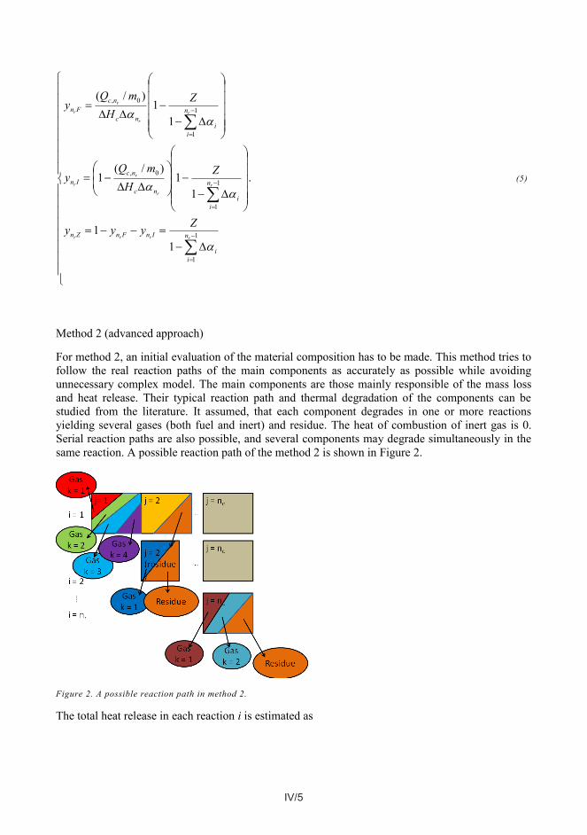
IV/5

1

1

1

1

0,

1

1

0,

11

11

)/(1

11

)/(

rrrr

r

r

r

r

r

r

r

r

n

ii

InFnZn

n

ii

nc

ncIn

n

ii

nc

ncFn

Zyyy

ZH

mQy

ZH

mQy

. (5)

Method 2 (advanced approach)

For method 2, an initial evaluation of the material composition has to be made. This method tries to follow the real reaction paths of the main components as accurately as possible while avoiding unnecessary complex model. The main components are those mainly responsible of the mass loss and heat release. Their typical reaction path and thermal degradation of the components can be studied from the literature. It assumed, that each component degrades in one or more reactions yielding several gases (both fuel and inert) and residue. The heat of combustion of inert gas is 0. Serial reaction paths are also possible, and several components may degrade simultaneously in the same reaction. A possible reaction path of the method 2 is shown in Figure 2.

Figure 2. A possible reaction path in method 2.

The total heat release in each reaction i is estimated as

IV/6 IV/7

cHmq . (10)

The heat release rate could be measured also directly by allowing gas phase calculation. However, then the grid cell size would be important parameter for the accuracy of the results, and the calculation would become significantly slower. The domain should also be divided to inert and oxidative ambient, which would increase the domain size even further. Therefore, this simplistic method for MCC experiment is chosen.

When the simulated TGA and MCC results are compared, it can be observed that in FDS the high heating rates move the reaction to higher temperatures. This behaviour can be observed in the experiments as well, but not nearly as much. The sample is in thermal equilibrium with the furnace, as can be observed in Figure 3 a. However, the increasing the heating rate of a simulation from 10 K/min to 60 K/min moves the curve about 50 K to higher temperatures (Figure 3b). This can be explained with the kinetic parameters. Sometimes, the reaction is slow compared to the heating rate. Although the reaction rate of the thermal degradation reaction is independent on the reaction rate, the temperature of the sample increases faster than the reaction can occur. Therefore at high heating rates it seems like the reaction has moved to higher temperatures.

a) b) Figure 3. Results of TGA/MCC simulation. a) Comparison of furnace and sample temperature at 60 K/min. b) TGA at 10 and 60 K/min.

In cone calorimeter experiments usually the cable is tested as whole, not divided into components as in the small scale experiments. The cables and all other complex structures are modelled as rectangular slabs. That works relatively well in coarse applications, but the solution is always limited by the grid size. Also the geometry is strongly simplified when the cylindrical object consisting of multiple components is treated as a laminate of separate, rectangular layers. This model has a domain of 0.3x0.3x0.4 m3 and grid size of 5 cm. The grid size is quite coarse but it should be similar to the one in the final application. The cone heater is modelled as an external heat flux (50 kW/m2) directed to the surface of the sample. The structure of the layers is symmetric.

MATERIALS

Generic materials

Three generic materials are developed. These samples represent ideal samples, where all reaction steps are well-defined and known. They do not correspond to any real material, and the parameters are listed only for completeness. Generic sample 1 is used to verify the calculations and simulation methods in a very simple case. The Generic sample 2 is made for verification with a more complex case where the first reaction has a small mass loss with high heat of combustion, and the second

c jpn

j

n

kkckjijii HyYQ

1 1,,,,1

;

ˆ , (6)

where Yi,j is the remaining mass fraction of the component j after reaction i. It is calculated from the initial mass fraction (Y0,j) as

i

iijZjiiji YyY

1,0,,, . (7)

The estimate for the conversion (or mass loss) is

c jpn

j

n

kjikji Yy

1 1,1,,

,

. (8)

The composition (initial mass fractions) can be solved by minimizing the error between the measured values and the calculated estimates as in

rn

i i

ii

i

ii

mQ

QmQ

aaa

10

0

ˆˆ

min . (9)

This optimization problem can be solved e.g. using Matlab (function fminsearch) or Excel (solver). The solutions of the software depend strongly on the initial values. Therefore a Matlab script was generated to test several random initial values from the pre-defined range. The solution with smallest error is then selected as the final solution. The script is very fast to run; the time to perform 1000 iterations is few minutes.

The original mass fractions can also have some constrains according to the typical concentrations in similar applications. Sometimes the components or their products may react together resulting different reaction paths than the components individually. Also the reaction rate and other experimental circumstances are known to affect on gas and residue yields.

Numerical simulations

For verification and validation purposes, the TGA, MCC and cone calorimeter experiments were modelled using Fire Dynamics Simulator (FDS). All the numerical simulations are performed using FDS version 6.0 (release candidate 4, svn 15111) [8].

If the thermal equilibrium is maintained in TGA, it can be simulated using a 0-dimensional model. In order to make a 0-dimensional model of the sample with FDS, which is basically a 2 or 3-dimensional flow solver coupled with 1-dimensional pyrolysis model, the physical dimensions of the TGA were significantly altered to decouple the gas phase conditions from the sample response. In practice, the TGA sample modelled as a 0.1 mm thick slab with surface area of 2 m2. The dimensions of the simulation domain were 4 m x 1 m x 1 m. All the gas phase reactions were prevented (nitrogen ambient), thus removing the dependence of the simulation on the gas phase cell size. The surrounding walls were heated linearly according to a slow, pre-determined heating rate from 20°C to 820°C. The thickness of the sample was small enough to keep it in thermal equilibrium with the environment. This was verified by measuring the temperatures of both the sample and the walls. The mass of the sample was monitored during the heating.

MCC experiment is identical to the TGA model in geometry, sample definition and omitting the gas phase calculation. The heat release rate is calculated as

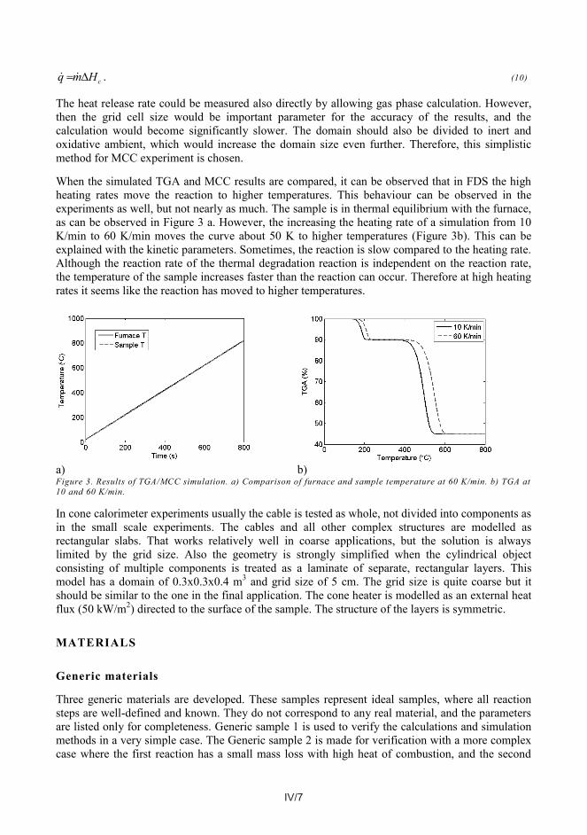
IV/7

cHmq . (10)

The heat release rate could be measured also directly by allowing gas phase calculation. However, then the grid cell size would be important parameter for the accuracy of the results, and the calculation would become significantly slower. The domain should also be divided to inert and oxidative ambient, which would increase the domain size even further. Therefore, this simplistic method for MCC experiment is chosen.

When the simulated TGA and MCC results are compared, it can be observed that in FDS the high heating rates move the reaction to higher temperatures. This behaviour can be observed in the experiments as well, but not nearly as much. The sample is in thermal equilibrium with the furnace, as can be observed in Figure 3 a. However, the increasing the heating rate of a simulation from 10 K/min to 60 K/min moves the curve about 50 K to higher temperatures (Figure 3b). This can be explained with the kinetic parameters. Sometimes, the reaction is slow compared to the heating rate. Although the reaction rate of the thermal degradation reaction is independent on the reaction rate, the temperature of the sample increases faster than the reaction can occur. Therefore at high heating rates it seems like the reaction has moved to higher temperatures.

a) b) Figure 3. Results of TGA/MCC simulation. a) Comparison of furnace and sample temperature at 60 K/min. b) TGA at 10 and 60 K/min.

In cone calorimeter experiments usually the cable is tested as whole, not divided into components as in the small scale experiments. The cables and all other complex structures are modelled as rectangular slabs. That works relatively well in coarse applications, but the solution is always limited by the grid size. Also the geometry is strongly simplified when the cylindrical object consisting of multiple components is treated as a laminate of separate, rectangular layers. This model has a domain of 0.3x0.3x0.4 m3 and grid size of 5 cm. The grid size is quite coarse but it should be similar to the one in the final application. The cone heater is modelled as an external heat flux (50 kW/m2) directed to the surface of the sample. The structure of the layers is symmetric.

MATERIALS

Generic materials

Three generic materials are developed. These samples represent ideal samples, where all reaction steps are well-defined and known. They do not correspond to any real material, and the parameters are listed only for completeness. Generic sample 1 is used to verify the calculations and simulation methods in a very simple case. The Generic sample 2 is made for verification with a more complex case where the first reaction has a small mass loss with high heat of combustion, and the second

IV/8 IV/9

Q/m0 31.5 4.5 1.75 13.02 5.88

PVC sheath

Real plasticized PVC can be significantly more complex than the generic example presented above. Therefore the methods are applied to a real thermoplastic cable with PVC sheath and PE insulation. The cable is the number #701 in the Christifire campaign (GENERAL CABLE® BICC® BRAND SUBSTATION CONTROL CABLE 7/C #12AWG 600V 30 MAY 2006). It has 7 conductor and diameter of 14 mm. All the other details can be found from the ref. [9]. The experimental data set included TGA results at 10 K/min and three repeated MCC results at 60 K/min for sheath and insulation. The experimental small scale results are listed in Table 2. In addition, cone calorimeter results at 25 KW/m2, 50 KW/m2 and 75 KW/m2 were available. The experimental results for the PVC sheath are shown in Figure 5. An average of the three repetitions of the MCC experiment was used.

Table 2. Experimental results for PVC sheath and PE insulation of cable #701.

Sheath Insulation Reac 1 Reac 2 Reac 3 Reac 1 Reac 2 Reac 3

Δα 0.600 0.137 0.040 0.570 0.120 0.052 Q/m0 (MJ/kg) 9.195 4.905 0.000 8.233 4.770 0.000

Figure 5. Experimental TGA (10 K/min) and MCC (60 K/min) results for PVC sheath. The experimental results are slightly filtered.

Understanding the basics of PVC blend degradation is important if more accurate reaction path is required. The theoretical background of the degradation of PVC and the most significant additives is therefore briefly presented here.

The thermal degradation of pure and plasticized PVC has been studied widely in the literature, experimentally ([10]-[16]) and numerically ([15]-[21]). Overall, the thermal degradation of the PVC is a two stage process. The first reaction around 320 °C is often called dehydrochlorination reaction, because it is mainly responsible of release of HCl. The remaining polyene structure starts degrading immediately releasing small amounts of aromatic hydrocarbons, mainly benzene. The second major reaction occurs around 450 °C, and is the pyrolysis of the polyene residue. The main product of this reaction is toluene. [10],[12],[17] Studied in vacuum [16], the mass loss of the first reaction was 64

reaction high mass loss with low heat of combustion. The accuracy of the reaction path for a PVC-like material is assessed with Generic sample 3. Other than kinetic parameters are same for all the samples and components, including char (ε = 1.0, cp = 1.0 kJ/kg·K, k = 1.0 W/m·K, ρ0 = 100 kg/m3, ΔH = 0 kJ/kg).

Generic 1 is the simplest test case with only one reaction step. It yields 0.9 of the mass fuel gas with heat of combustion 35 MJ/kg. The parameters are listed in Table 1 .

The second test case, Generic 2, yields little mass and lots of energy at the first reaction step, and the second releases lots of mass and little energy. The reaction parameters are listed in Table 1 and visually shown in Figure 4a.

For testing the method for more complex sample, a third generic material (Generic 3) is used. The kinetics or other parameters do not represent any specific material, and the kinetic parameters of components 1 and 3 are identical to those of Generic 2. The reaction path resembles the one of plasticized PVC. It has two initial components (Comp 1 and Comp 2) as the PVC polymer and the plasticizer. They start to thermally degrade in close to the same temperatures. The earlier reaction yields some fuel gas, inert gas (as Hydrocloric acid (HCl) in PVC) and residual polymer that degrades further in higher temperatures. The second initial component releases fuel gas and no residue during the first reaction step. All the parameters are listed in Table 1 and the simulated results are shown in Figure 4b.

a)

b)

Figure 4. Generic samples. TGA results are shown on the left axes and MCC results on the right. a) Generic 2 sample. b) Generic 3 sample.

Table 1. Reaction parameters and resulting mass loss and energy release of each reaction for the generic samples 1 , 2 and 3.

Generic 1 Generic 2 Generic 3 Comp 1 Comp 1 Comp 2 Comp 1 Comp 2 Comp 3

Mass fraction in virgin material 1.0 0.5 0.5 0.7 0.3 0.0 A (s-1) 1.0·1010 1.0·1015 1.0·1010 1.0·1015 1.0·1016 1.0·1010 E (J/mol) 1.6·105 1.48·105 1.8·105 1.48·105 1.55·105 1.8·105 gas yield 0.9 (fuel) 0.2 (fuel) 0.1 (fuel)

0.8 (inert) 0.02 (fuel) 0.58 (inert) 1.0 (fuel) 0.6 (fuel)

ΔHc (MJ/kg) 35 45 35 30 35 42 Residue? Char Char Char Comp 3 No residue Char Peak Temperature (°C) at 10 K/min 420 180 500 180 180 500

Δα 0.9 0.1 0.45 0.72 0.17

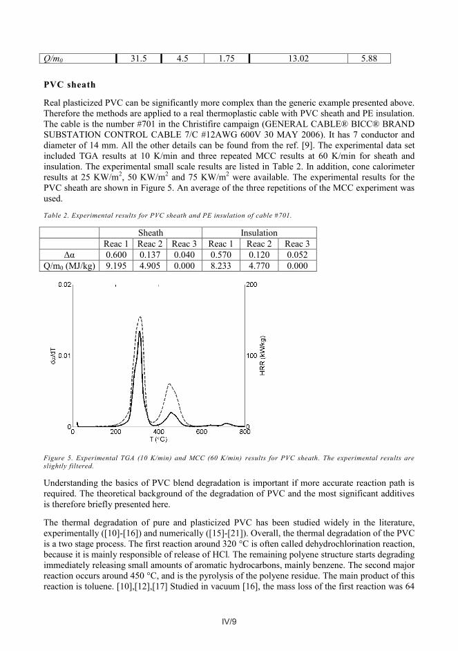
IV/9

Q/m0 31.5 4.5 1.75 13.02 5.88

PVC sheath

Real plasticized PVC can be significantly more complex than the generic example presented above. Therefore the methods are applied to a real thermoplastic cable with PVC sheath and PE insulation. The cable is the number #701 in the Christifire campaign (GENERAL CABLE® BICC® BRAND SUBSTATION CONTROL CABLE 7/C #12AWG 600V 30 MAY 2006). It has 7 conductor and diameter of 14 mm. All the other details can be found from the ref. [9]. The experimental data set included TGA results at 10 K/min and three repeated MCC results at 60 K/min for sheath and insulation. The experimental small scale results are listed in Table 2. In addition, cone calorimeter results at 25 KW/m2, 50 KW/m2 and 75 KW/m2 were available. The experimental results for the PVC sheath are shown in Figure 5. An average of the three repetitions of the MCC experiment was used.

Table 2. Experimental results for PVC sheath and PE insulation of cable #701.

Sheath Insulation Reac 1 Reac 2 Reac 3 Reac 1 Reac 2 Reac 3

Δα 0.600 0.137 0.040 0.570 0.120 0.052 Q/m0 (MJ/kg) 9.195 4.905 0.000 8.233 4.770 0.000

Figure 5. Experimental TGA (10 K/min) and MCC (60 K/min) results for PVC sheath. The experimental results are slightly filtered.

Understanding the basics of PVC blend degradation is important if more accurate reaction path is required. The theoretical background of the degradation of PVC and the most significant additives is therefore briefly presented here.

The thermal degradation of pure and plasticized PVC has been studied widely in the literature, experimentally ([10]-[16]) and numerically ([15]-[21]). Overall, the thermal degradation of the PVC is a two stage process. The first reaction around 320 °C is often called dehydrochlorination reaction, because it is mainly responsible of release of HCl. The remaining polyene structure starts degrading immediately releasing small amounts of aromatic hydrocarbons, mainly benzene. The second major reaction occurs around 450 °C, and is the pyrolysis of the polyene residue. The main product of this reaction is toluene. [10],[12],[17] Studied in vacuum [16], the mass loss of the first reaction was 64

IV/10 IV/11

Table 3. For both methods the reaction specific mass loss and heat release are calculated correctly with these parameters. Method 2 only slightly (3 %) overestimates the mass loss of the reaction 2 (0.46), but the total heat release is exactly 1.75 MJ/kg.

Table 3. Estimation results and estimation boundaries for method 2 of sample Generic 2.

yI11 yF11 yI22 yF22 ΔHc,11 (MJ/kg) ΔHc,22 (MJ/kg) Exact value 0.00 0.20 0.80 0.10 45.00 35.00 Method 1 0.03 0.97 0.46 0.04 46.45 46.45 Method 2 0.01 0.19 0.81 0.12 47.02 30.07 Est. boundaries [0,1] [0,0.3] [0,1] [0,0.3] [30, 50] [30, 50]

The Generic 3 sample undergoes three fuel yielding reactions. Two first reactions (Comp 1 and Comp 2) are overlapping and inseparable in time or temperature. The net energy release in the first reaction should be (according to Table 1) 13.02 MJ/kg and in the second 5.88 MJ/kg, making the total heat release of the sample 18.90 MJ/kg. The corresponding mass losses should be 0.72 and 0.17. An integral over the peaks confirm these results.

For Method 1, we assume that the heat of combustion of the fuel gas is 40 MJ/kg. For the first reaction, the parameters are Qc,1/m0 = 13.02 MJ/kg, Δα1 = 0.72 and ΔHc = 40 MJ/kg. According to eq. (4), the fuel yield (y1F) is 0.45 (and the yield of the inert gas is therefore 0.55). For the second reaction, we have to take the char yield into account. The total char yield of the material (Z) is 0.11. The fraction of the fuel of all the gas released in the second reaction is by eq. (4) 0.865. The yields are then calculated as in eq. (5)

39.008.053.01y

0.0872.01

11.01)865.01(y

0.5372.01

11.01865.0

2Z

2I

2Fy

.

The results are summarized in Table 4.

Table 4. The yields and mass fractions for generic sample 3 using Method 1.

yF yI yZ Y Reaction 1 0.45 0.55 0.0 0.72 Reaction 2 0.53 0.08 0.39 0.28

For method 2 we assume that the material is a PVC polymer with some plasticizer. We set the estimation boundaries as listed in Table 5. The estimation problem was solved using a Matlab function and a script that tried random initial values and chose the values that gave the smallest error. The iteration with random initial values was performed 5000 times, and the best solution gave an error of 5.8·10-8. The values for the final estimation results can be seen in Table 5. The results are relatively near the target values considering the width of the estimation boundaries.

%, which is higher than the stoichiometric value 58.7 %. Therefore the amount of benzene release in the first reaction was 5.3%. The mass loss of the second reaction was 30.3 % leaving 5.7 % residue.

Various additives have effect on the thermal degradation of PVC. The most important additive in many PVC applications (including cables) is the plasticizer. The concentrations can be as high as 100 phr (parts per hundred parts of resin). There are several commercial plasticizers available, and one of the most commonly studied of them is Di-2-ethylhexyl phthalate (DOP). Marcilla and Beltrán compared pure samples of DOP and PVC resin to mixtures at different concentrations and heating rates [15]. The plasticizer degrades around the same temperatures as the dehydrochlorination reaction, but carefully looking two peaks can be observed; DOP evaporates slightly before HCl. When the peak temperatures are compared, it can be seen that in mixture the reactions are closer to each other, almost overlapping: DOP evaporates slightly later, and HCl slightly earlier than separately. Low concentrations of DOP decrease this effect. Also, at higher heating rates the decrease in resin degradation temperature is not as significant as at the lower heating rates. One explanation for the decreasing HCl release temperature is that when the DOP evaporates, it leaves holes to the polymer blend structure. These holes are the initiation centres of the dehydrochlorination process and the reaction becomes faster. Another explanation is that the radicals formed around 300 °C at the DOP evaporation promote the reaction. DOP is also known to partially inhibit the release of the aromatics formation. [12],[13],[15]

PVC blend also includes some amount of fillers. Calcium Carbonate (CaCO3) is the most commonly used with PVC. It is used to improve the impact resistance and thermal stability. Typical concentrations are 20-30 wt% in rigid and 30-40 wt% in flexible PVC. [22] It may react with HCl producing calcium chloride. It also degrades at high temperatures (above 840 °C) producing CO2 and H2O.

Other significant additives are stabilizers and metal oxides, although their concentrations are not very high. The stabilizers do not affect on the degradation temperatures, but they seem to inhibit the formation of the HCl. In higher concentrations (> 1 phr) they also seem to inhibit the formation of benzene and toluene [13]. Metal oxides suppress the amount of released aromatic hydrocarbons. Some oxides also lower the temperature of the dehydrochlorination reaction. Those metal oxides that suppress most benzene formation also promote char under nitrogen ambient. [10] The role of these additives is not investigated in this paper.

The insulation layer is nominally a polyethylene (PE) blend. Pure PE degrades around 400-500 °C without leaving residue. The additives are assumed to be similar to those of PVC for simplicity. [23]

RESULTS

Generic samples

The calculation and simulation methods were first verified by using the Generic 1 sample. The results show that the correct amount of heat can be allocated to each reaction using both methods. Additionally, it showed that the FDS model indeed calculates the mass and heat release as expected.

The Generic 2 sample undergoes two reactions. Both of them yield fuel and residue, the second also inert gas. The experimental results and the target values were listed in Table 1. These results are confirmed by integrating over the reaction steps of the FDS results. The mass fractions of the components are assumed known (0.5 for both components), and the other parameters are listed in

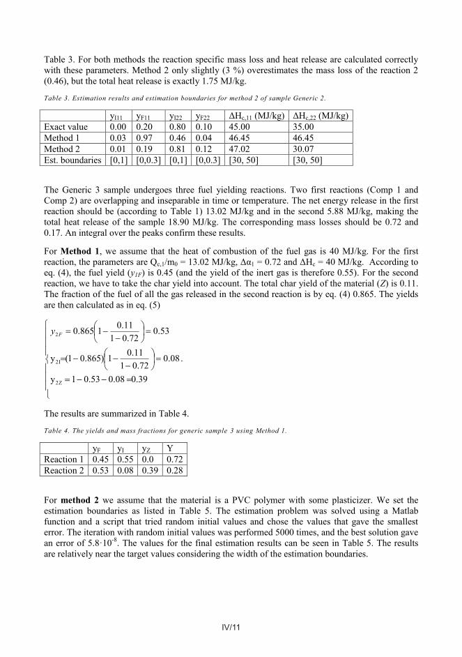
IV/11

Table 3. For both methods the reaction specific mass loss and heat release are calculated correctly with these parameters. Method 2 only slightly (3 %) overestimates the mass loss of the reaction 2 (0.46), but the total heat release is exactly 1.75 MJ/kg.

Table 3. Estimation results and estimation boundaries for method 2 of sample Generic 2.

yI11 yF11 yI22 yF22 ΔHc,11 (MJ/kg) ΔHc,22 (MJ/kg) Exact value 0.00 0.20 0.80 0.10 45.00 35.00 Method 1 0.03 0.97 0.46 0.04 46.45 46.45 Method 2 0.01 0.19 0.81 0.12 47.02 30.07 Est. boundaries [0,1] [0,0.3] [0,1] [0,0.3] [30, 50] [30, 50]

The Generic 3 sample undergoes three fuel yielding reactions. Two first reactions (Comp 1 and Comp 2) are overlapping and inseparable in time or temperature. The net energy release in the first reaction should be (according to Table 1) 13.02 MJ/kg and in the second 5.88 MJ/kg, making the total heat release of the sample 18.90 MJ/kg. The corresponding mass losses should be 0.72 and 0.17. An integral over the peaks confirm these results.

For Method 1, we assume that the heat of combustion of the fuel gas is 40 MJ/kg. For the first reaction, the parameters are Qc,1/m0 = 13.02 MJ/kg, Δα1 = 0.72 and ΔHc = 40 MJ/kg. According to eq. (4), the fuel yield (y1F) is 0.45 (and the yield of the inert gas is therefore 0.55). For the second reaction, we have to take the char yield into account. The total char yield of the material (Z) is 0.11. The fraction of the fuel of all the gas released in the second reaction is by eq. (4) 0.865. The yields are then calculated as in eq. (5)

39.008.053.01y

0.0872.01

11.01)865.01(y

0.5372.01

11.01865.0

2Z

2I

2Fy

.

The results are summarized in Table 4.

Table 4. The yields and mass fractions for generic sample 3 using Method 1.

yF yI yZ Y Reaction 1 0.45 0.55 0.0 0.72 Reaction 2 0.53 0.08 0.39 0.28

For method 2 we assume that the material is a PVC polymer with some plasticizer. We set the estimation boundaries as listed in Table 5. The estimation problem was solved using a Matlab function and a script that tried random initial values and chose the values that gave the smallest error. The iteration with random initial values was performed 5000 times, and the best solution gave an error of 5.8·10-8. The values for the final estimation results can be seen in Table 5. The results are relatively near the target values considering the width of the estimation boundaries.

IV/12 IV/13

Application to a real PVC sheath

Small scale model

As seen in Figure 5, the TGA results show three reaction peaks, MCC results only two. As listed in Table 2, the measured heat releases are 9.195 MJ/kg in the first reaction and 4.905 MJ/kg in the second. The mass losses are 0.6, 0.137 and 0.04, correspondingly. The kinetic parameters (A, E, N) were estimated using Genetic Algorithm (GA) ([2],[9]) for both methods (different reaction paths) separately. The kinetic parameters are known to compensate the other parameter values so that there may be several sets of equally fitting parameters. To minimize this effect, the parameters should be estimated at several heating rates. Unfortunately, the experimental data set only included on heating rate at 10 K/min. However, from the MCC results (at 60 K/min) it can be seen, that the reactions happen almost simultaneously as seen in Figure 5. Therefore the parameters are estimated at these two heating rates, using the same experimental results from 10 K/min.

The reaction path parameters were estimated similarly for the insulating material that was known to be PE. It had similarly three mass loss peaks, the third one without heat release. The mass losses of the reactions were 0.57, 0.12 and 0.052. The heat releases of the two first reactions were 8.233 MJ/kg and 4.77 MJ/kg.

Method 1: The fuel in this model was assumed to be propane (46.45 MJ/kg) and the inert gas water vapour. The fuel yields are calculated according eq. (4) and eq. (5) and the results are listed in Table 6. The reaction path and the kinetic parameters are shown in Figure 7. The comparison between experimental and simulated small scale results are seen in Figure 9.

With similar assumptions of the fuel gas as for the sheath material, the fuel yields of the insulation material are 0.31 and 0.86 in two first reactions. The third reaction does not yield fuel gas, and residue yield is 0.83. The kinetic parameters are listed in Table 8.

Figure 7. Reaction path and kinetic parameters for the PVC sheath using Method 1.

Table 5. Estimation boundaries, initial values and the final results for the Generic 3 sample. The first subscript denotes to reaction and second to component (PVC = 1, plasticizer = 2) .

Variable Boundaries Initial value used Target value Estimation result Error Y1 (“PVC”) [0.5, 0.8] 0.59 0.70 0.70 0 % Y2 (“Plasticizer”) - 0.41 0.30 0.30 0 % yI11 [0.57, 0.61] 0.58 0.58 0.60 -3 % yF11 [0, 0.05] 0.00 0.02 0.00 100 % yF12 [0.5, 0.9] 0.67 0.60 0.61 -2 % ΔHc11 (MJ/kg) [20, 45] 30.27 30.0 27.60 8 % ΔHc12 (MJ/kg) [20, 45] 34.28 35.0 34.59 1 % ΔHc21 (MJ/kg) [20, 45] 36.05 42.0 43.04 -2 %

The results with Method 1 and Method 2 were next tested by investigating if the resulting parameters can reproduce the mass loss and heat release characteristics of the generic data. This was done by calculating the TGA and MCC experiments using both reaction paths. The kinetic parameters are assumed to be known exactly (for Method 1, only those of the Comp 1 are used for the first reaction). The results confirm that although the reaction paths and assumptions are different, the essential information (mass loss and heat release) can be repeated correctly using both methods. The results are shown in Figure 6.

In addition to the mass and energy calculation, the capability of method 2 was validated by comparing the estimated and target values. The errors between these two values are listed in Table 5. In general, the estimated values are within 10 % to the real ones. However, the greatest error is with the fuel yield of the Comp 1 in reaction 1. As the amount of fuel from the PVC is very small, this error is irrelevant.

a)

b)

Figure 6. Verification of the estimation results. a) Mass loss (TGA at 10 K/min in N2). b) Energy release (MCC at 60 K/min in air).

IV/13

Application to a real PVC sheath

Small scale model

As seen in Figure 5, the TGA results show three reaction peaks, MCC results only two. As listed in Table 2, the measured heat releases are 9.195 MJ/kg in the first reaction and 4.905 MJ/kg in the second. The mass losses are 0.6, 0.137 and 0.04, correspondingly. The kinetic parameters (A, E, N) were estimated using Genetic Algorithm (GA) ([2],[9]) for both methods (different reaction paths) separately. The kinetic parameters are known to compensate the other parameter values so that there may be several sets of equally fitting parameters. To minimize this effect, the parameters should be estimated at several heating rates. Unfortunately, the experimental data set only included on heating rate at 10 K/min. However, from the MCC results (at 60 K/min) it can be seen, that the reactions happen almost simultaneously as seen in Figure 5. Therefore the parameters are estimated at these two heating rates, using the same experimental results from 10 K/min.

The reaction path parameters were estimated similarly for the insulating material that was known to be PE. It had similarly three mass loss peaks, the third one without heat release. The mass losses of the reactions were 0.57, 0.12 and 0.052. The heat releases of the two first reactions were 8.233 MJ/kg and 4.77 MJ/kg.

Method 1: The fuel in this model was assumed to be propane (46.45 MJ/kg) and the inert gas water vapour. The fuel yields are calculated according eq. (4) and eq. (5) and the results are listed in Table 6. The reaction path and the kinetic parameters are shown in Figure 7. The comparison between experimental and simulated small scale results are seen in Figure 9.

With similar assumptions of the fuel gas as for the sheath material, the fuel yields of the insulation material are 0.31 and 0.86 in two first reactions. The third reaction does not yield fuel gas, and residue yield is 0.83. The kinetic parameters are listed in Table 8.

Figure 7. Reaction path and kinetic parameters for the PVC sheath using Method 1.

IV/14 IV/15

Table 7. Estimation boundaries, initial values and the final estimated values of the PVC sheath using Method 2.

Estimation boundaries Initial values Estimation result Y1 [0.2, 0.7] 0.508 0.514 Y2 [0.1, 0.5] 0.323 0.268 Y3 - 0.169 0.218 yI11 [0.57,0.61] 0.606 0.602 yF11 [0, 0.07] 0.040 0.043 yF12 [0.5, 0.9] 0.786 0.751 yI13 [0.05, 0.3] 0.186 0.184 ΔHc11 (MJ/kg) [25, 50] 48.9 49.1 ΔHc12 (MJ/kg) [25, 50] 31.2 35.8 ΔHc21 (MJ/kg) [25, 50] 32.1 30.2

Table 8. The kinetic parameters for PVC sheath and insulation using Method 1 and Method 2.

Material Method Component (i) Reaction (j)

A (s-1) E (mol/kJ) N

Sheath (PVC)

Method 1 i = j= 1 3.6·1021 2.4·105 2.87 i = j = 2 1.2·1029 3.8·105 4.10 i = j = 3 5.1·1021 3.0·105 2.67

Method 2 i = 1,2, j = 1 2.1·1026 2.8·105 3.69 i = 1, j = 2 2.0·1025 3.2·105 4.91 i = 3, j = 3 9.8·1024 2.9·105 0.96

Insulation (PE)

Both methods

i = j = 1 1.26·1025 2.7·105 3.20 i = j = 2 1.9·1027 3.6·105 3.7 i = j =3 1.6·1012 2.1·105 4.41

a)

b) Figure 9. Comparison of the experimental and simulated results for r eal PVC sheath. a) TGA. b) MCC.

Bench scale model

The cone calorimeter experiments were performed at 25, 50 and 75 kW/m2 heat fluxes. The experimental results are listed at Table 9. The mass fractions of the components were 0.24 (sheath), 0.18 (insulation) and 0.58 (conductor). Conductor is non-combustible. The total mass loss of the sheath is 77.7 % and of insulation 74.2 % and total heat release 14.1 MJ/kg and 13.0 MJ/kg,

Table 6. Estimation results for PVC sheath and PE insulation using Method 1.

Reaction i

Yi yFi yIi yRi

Sheath (PVC)

1 0.600 0.33 0.67 0.00 2 0.137 0.77 0.23 0.00 3 0.263 0.00 0.15 0.85

Insulation (PE)

1 0.57 0.31 0.69 0.00 2 0.12 0.86 0.14 0.00 3 0.31 0.00 0.17 0.83

Method 2: The reaction path of the real PVC sheath was assumed similar to the Generic 2 sample, and the third additional reaction (with no measured heat release) was assumed to be due to CaCO3 thermal degradation. The estimation boundaries are listed in Table 7. The optimization was performed using the Matlab script mentioned before. In 5000 iterations, the minimum was found with error (eq. (9)) of 2.4·10-7. The resulting values are listed in Table 7 and the reaction path and kinetic parameters are shown in Figure 8. The comparison between experimental and simulated small scale results are shown in Figure 9.

The insulating material was known to be PE. Pure PE is thermoplastic and therefore does not yield residue. The first reaction corresponds to the temperature range of the plasticizer, and second to the degradation of the PE. The third reaction is again assumed to be due to CaCO3. As the two fuel yielding components do not yield any char (at least, not in their pure form), the mass losses of the reactions are used as the mass fractions of the components. The calculation of the heat of combustions is very straight-forward and they can be calculated using eq. (4). As result, the heats of combustions for two first reactions are 14.45 MJ/kg and 39.73 MJ/kg, respectively. The residue yield of the last reaction is 0.83.

Figure 8. Reaction path and kinetic parameters for a PVC sheath using Method 2.

IV/15

Table 7. Estimation boundaries, initial values and the final estimated values of the PVC sheath using Method 2.

Estimation boundaries Initial values Estimation result Y1 [0.2, 0.7] 0.508 0.514 Y2 [0.1, 0.5] 0.323 0.268 Y3 - 0.169 0.218 yI11 [0.57,0.61] 0.606 0.602 yF11 [0, 0.07] 0.040 0.043 yF12 [0.5, 0.9] 0.786 0.751 yI13 [0.05, 0.3] 0.186 0.184 ΔHc11 (MJ/kg) [25, 50] 48.9 49.1 ΔHc12 (MJ/kg) [25, 50] 31.2 35.8 ΔHc21 (MJ/kg) [25, 50] 32.1 30.2

Table 8. The kinetic parameters for PVC sheath and insulation using Method 1 and Method 2.

Material Method Component (i) Reaction (j)

A (s-1) E (mol/kJ) N

Sheath (PVC)

Method 1 i = j= 1 3.6·1021 2.4·105 2.87 i = j = 2 1.2·1029 3.8·105 4.10 i = j = 3 5.1·1021 3.0·105 2.67

Method 2 i = 1,2, j = 1 2.1·1026 2.8·105 3.69 i = 1, j = 2 2.0·1025 3.2·105 4.91 i = 3, j = 3 9.8·1024 2.9·105 0.96

Insulation (PE)

Both methods

i = j = 1 1.26·1025 2.7·105 3.20 i = j = 2 1.9·1027 3.6·105 3.7 i = j =3 1.6·1012 2.1·105 4.41

a)

b) Figure 9. Comparison of the experimental and simulated results for r eal PVC sheath. a) TGA. b) MCC.

Bench scale model

The cone calorimeter experiments were performed at 25, 50 and 75 kW/m2 heat fluxes. The experimental results are listed at Table 9. The mass fractions of the components were 0.24 (sheath), 0.18 (insulation) and 0.58 (conductor). Conductor is non-combustible. The total mass loss of the sheath is 77.7 % and of insulation 74.2 % and total heat release 14.1 MJ/kg and 13.0 MJ/kg,

IV/16 IV/17

Table 10. Thermal parameters of cable 701.

Method 1 Method 2 Polymer Plasticizer CaCO3

She

ath

Reaction 1

k (W/(mK)) 0.147 0.146 0.185 0.48 cp (kJ/(kgK)) 3.22 3.4 2.8 3.5 ΔH (kJ/kg) 1607 206 1112 1669 ε 0.7 1.0 1.0 1.0

Reaction 2

k (W/(mK)) 0.175 0.2 - - cp (kJ/(kgK)) 3.45 2.26 - - ΔH (kJ/kg) 1425 1783 - - ε 1.0 1.0 - -

Reaction 3

k (W/(mK)) 0.103 - - - cp (kJ/(kgK)) 3.5 - - - ΔH (kJ/kg) 43 - - - ε 1.0 - - -

Residue

ρ (kg/m3) 344 70 274 k (W/(mK)) 0.122 0.188 - 0.188 cp (kJ/(kgK)) 3.5 2.0 - 2.0 ε 0.85 1.0 - 1.0

Insu

latio

n

Reaction 1


Reaction 2

k (W/(mK)) 1.0 - 0.59 - cp (kJ/(kgK)) 3.4 - 3.0 - ΔH (kJ/kg) 1516 - 691 - ε 1.0 - 1.0 -

Reaction 3

k (W/(mK)) 0.087 - - 0.285 cp (kJ/(kgK)) 2.74 - - 2.9 ΔH (kJ/kg) 445 - - 353 ε 1.0 - - 1.0

Residue

297 - - 297 k (W/(mK)) 0.01 - - 0.338 cp (kJ/(kgK)) 1.29 - - 1.29 ε 1.0 - - 1.0

respectively. Multiplying by mass fractions and the initial mass 270 g, the mass loss is 84.8 g (32 %) and the total heat release 1.52 MJ. The effective heat of combustion (total heat release scaled by the mass loss) is then 17.9 MJ/kg. This is less than in cone calorimeter experiments at 25 and 50 kW/m2. The extra heat released is related to the oxidation of char. This phenomenon is addressed in the next section.

Table 9. Experimental cone calorimeter results .

25 kW/m2 50 kW/m2 75 kW/m2 m0 (g) 263.9 269.0 262.2 Δm (g) 71.0 91.2 89.0 Δm/m0 (g/g) 0.27 0.34 0.34 Qtot (MJ) 1.92 1.71 1.59 ΔHc, eff (MJ/kg) 27 18.75 17.9

The cone calorimeter models were developed based on the small scale results and mass fractions. The results are listed in Table 10 and graphically presented in Figure 10. The cone calorimeter models where calculated using FDS 6 with 5 cm grid resolution. The parameters were fitted at 50 kW/m2 heat flux, and validated using results of 25 and 75 kW/m2 heat fluxes.

50 kW/m2 25 kW/m2 and 75 kW/m2

a)

b)

c)

d)

Figure 10. Cone calorimeter results for Method 1 and Method 2. a) Heat release rate at 50 kW/m 2. b) Heat release rate at other heat fluxes. c) Mass loss rate at 50 kW/m2. d) Mass loss rate at other heat fluxes.

IV/17

Table 10. Thermal parameters of cable 701.

Method 1 Method 2 Polymer Plasticizer CaCO3

She

ath

Reaction 1

k (W/(mK)) 0.147 0.146 0.185 0.48 cp (kJ/(kgK)) 3.22 3.4 2.8 3.5 ΔH (kJ/kg) 1607 206 1112 1669 ε 0.7 1.0 1.0 1.0

Reaction 2


Reaction 3

k (W/(mK)) 0.103 - - - cp (kJ/(kgK)) 3.5 - - - ΔH (kJ/kg) 43 - - - ε 1.0 - - -

Residue

ρ (kg/m3) 344 70 274 k (W/(mK)) 0.122 0.188 - 0.188 cp (kJ/(kgK)) 3.5 2.0 - 2.0 ε 0.85 1.0 - 1.0

Insu

latio

n

Reaction 1


Reaction 2

k (W/(mK)) 1.0 - 0.59 - cp (kJ/(kgK)) 3.4 - 3.0 - ΔH (kJ/kg) 1516 - 691 - ε 1.0 - 1.0 -

Reaction 3

k (W/(mK)) 0.087 - - 0.285 cp (kJ/(kgK)) 2.74 - - 2.9 ΔH (kJ/kg) 445 - - 353 ε 1.0 - - 1.0

Residue

297 - - 297 k (W/(mK)) 0.01 - - 0.338 cp (kJ/(kgK)) 1.29 - - 1.29 ε 1.0 - - 1.0

IV/18 IV/19

a)

b) Figure 12. Cone calorimeter results with oxidation at 50 kW/m2. a) Heat release rate. b) Mass loss rate.

Table 11. Parameters for surface oxidation of cable shea th.

Method 1 Method 2 22.9 % of initial mass

A (s-1) 6.0·1012 2.5·1010 E (kJ/kmol) 2.5·105 2.3·105 N 1.4 1.0 nO2 1.5 1.5 yF 0.34 0.34 k (W/m·K) 1.0 0.2 cp (kJ/kg·K) 1.0 2.5 ΔH (kJ/kg) 0 1500

ash k (W/m·K) 0.122 0.6 cp (kJ/kg·K) 3.5 3.0 ε 0.85 1.0

CONCLUSIONS

Unknown composition of the sample material is often a challenge in the pyrolysis and fire modelling. Since it is not practical to perform a complete chemical analysis of each material, alternative methods have been searched. An experimental tool, MCC, has been exploited for measuring the heat of combustion of each reaction and estimation of the sample composition.

Two new methods for combining MCC and TGA results were developed. First one is a simple and practical engineering solution that just measures the net heat release of each reaction. This approach is usually enough in order to make an accurate pyrolysis model. The second one has more ambitious goal to understanding better the sample material. It requires some knowledge about the chemical components and the degradation path of the material. This method may be more useful in the academic research projects than in engineering applications. Both methods were applied to two generic materials with known reaction paths and parameters, and to one real PVC mixture of an electric cable.

Surface oxidation

It was noticed that the heat release and mass loss in cone calorimeter was higher than according to small scale results should be. This was speculated to be due to surface oxidation, and this can be confirmed by comparing TGA results in air and nitrogen. In air the mass loss of the sheath is 7.7% higher than in nitrogen. This corresponds to 1.7 % (4.6 g) mass loss in the whole cable. The heat released in cone calorimeter is about 0.17 MJ more than that of the models. Dividing the heat by the mass loss gives heat of oxidation about 37 MJ/kg.

The newest version of FDS 6 is currently able to model the oxidation as function of available oxygen [8]. The reaction rate defined by Arrhenius parameters is multiplied by a function of oxygen volume fraction of the first gas cell

ijOiji nO

ijnijij X

RTE

Ar ,2

20exp

. (11)

In normal pyrolysis reaction order of oxidation is 0. Deeper under the surface the oxygen concentration depends on the diffusion depth, also defined by user. The parameters are found by comparing the model with the last reaction of TGA experiment in air. For method 1, the oxidation reaction is one parallel reaction more. For method 2, the char yielded by PVC and CaCO3 is converted into ash. The parameters of this reaction are listed in Table 10 and visually shown in Figure 11. The pyrolysis reactions do not fit exactly to the experimental data. Part of the reason may be the ignition model of FDS. In FDS, whenever oxygen is present, the fuel gas ignites. In real TGA this hardly happens, since the temperatures of most degradation steps are below the autoignition temperature. However, also in the experiment the fuel reacts with oxygen in some level, releasing heat. For these reasons, the only significant part of the curve is in the end, corresponding to the surface oxidation.

The cone calorimeter results are shown in Figure 12. It seems that the oxidation alone does not explain the different mass loss and heat release results in the cone calorimeter.

a)

b)

Figure 11. Implementing the oxidation reaction. a) TGA in air. b) Zoomed i n to the end of the experiment.

IV/19

a)

b) Figure 12. Cone calorimeter results with oxidation at 50 kW/m2. a) Heat release rate. b) Mass loss rate.

Table 11. Parameters for surface oxidation of cable shea th.

Method 1 Method 2 22.9 % of initial mass

A (s-1) 6.0·1012 2.5·1010 E (kJ/kmol) 2.5·105 2.3·105 N 1.4 1.0 nO2 1.5 1.5 yF 0.34 0.34 k (W/m·K) 1.0 0.2 cp (kJ/kg·K) 1.0 2.5 ΔH (kJ/kg) 0 1500

ash k (W/m·K) 0.122 0.6 cp (kJ/kg·K) 3.5 3.0 ε 0.85 1.0

CONCLUSIONS

Unknown composition of the sample material is often a challenge in the pyrolysis and fire modelling. Since it is not practical to perform a complete chemical analysis of each material, alternative methods have been searched. An experimental tool, MCC, has been exploited for measuring the heat of combustion of each reaction and estimation of the sample composition.

Two new methods for combining MCC and TGA results were developed. First one is a simple and practical engineering solution that just measures the net heat release of each reaction. This approach is usually enough in order to make an accurate pyrolysis model. The second one has more ambitious goal to understanding better the sample material. It requires some knowledge about the chemical components and the degradation path of the material. This method may be more useful in the academic research projects than in engineering applications. Both methods were applied to two generic materials with known reaction paths and parameters, and to one real PVC mixture of an electric cable.

IV/20 IV/21

11. Mountado, G., Puglisi, C. Evolution of Aromatics in the Thermal Degradation of Poly(vinyl chloride): A Mechanistic Study. Polymer Degradation and Stability 33 (1991) 229-262

12. Marcilla, A., Beltrán, M. PVC-plasticizer interactions during the thermal decomposition of PVC plastisols. Influence of the type of plastizicer and resin. Polymer Degradation and Stability 53 (1996) 261-268.

13. Jiménez, A., López, J., Vilaplana, J., Dussel, H.-J. Thermal degradation of plastisols. Effect of some additives on the evolution of gaseous products. Journal of Analytical and Applied Pyrolysis 40-41 (1997) 201-215.

14. Elakesh, E.O., Hull, T.R., Price, D., Milnes, G.J. Carty, P. Effect of Plasticizers on the Thermal Decomposition of Chlorinated Polyvinylchloride. Journal of Vinyl & Additive Technology (2005).

15. Marcilla, A., Beltrán, M. Effect of the plasticizer concentration and heating rate on the thermal decomposition behavior of PVC plastisols. Kinetic analysis. Polymer degradation and Stability 60 (1998) 1-10.

16. Miranda, R., Yang, J., Roy, C., Vasile, C. Vacuum pyrolysis of PVC I. Kinetic study. Polymer Degradation and Stability 64 (1999) 127-144.

17. Marcilla, A., Beltrán, M. Thermogravimetric kinetic study of poly(vinyl chloride) pyrolysis. Polymer Degradation and Stability 48 (1995) 219-229.

18. Marcilla, A., Beltrán, M. Kinetic models for the thermal decomposition of commercial PVC resins and plasticizers studied by thermogravimetric analysis. Polymer Degradation and Stability 53 (1996) 251-260.

19. Beltrán, M., Marcilla, A. Kinetic models for the thermal decomposition of PVC plastisols. Polymer Degradation and Stability 55 (1997) 73-87.

20. Kim, S. Pyrolysis kinetics of waste PVC pipe. Waste Management 21 (2001) 609-616.

21. Matala, A., Hostikka, S. Pyrolysis Modelling of PVC Cable Materials. Fire Safety Science 10 (2011).

22. Wypych, G. PVC Formulary. ChemTec Publishing. (2009) pp. 379.

23. Marcilla, A., Ruiz-Femenia, R., Hernández, J., García-Quesada, J.C. Thermal and catalytic pyrolysis of crosslinked polyethylene. Journal of Analytical Applied Pyrolysis 76 (2006) 254-259. doi:10.1016/j.jaap.2005.12.004

Both methods were verified to calculate the heat release of each reaction correctly. The method 2 was also validated by comparing the estimated and target values of the mass fractions, fuel yields and the heat of combustions of the reactions. The differences were very small considering that the parameters are known to compensate each other.

The methods 1 and 2 were finally used in the pyrolysis modelling of a real PVC cable. The results are realistic and predicting the small scale experiments accurately. The models were applied also in the bench scale using cone calorimeter results. The surface oxidation of char was also modelled. Surface oxidation is a significant phenomenon in the end of the cone calorimeter experiment and can be observed visually by the glowing surface. However, in the model this did not seem to make great difference because of the definition of the reaction paths.

Acknowledgements

The authors would like to thank Dr. Kevin McGrattan from NIST for the MCC and cone calorimeter results for cable #701 and Dr. Tuula Leskelä (Aalto University School of Science and Technology) for the TGA results. The work has been partially funded by the Nuclear Waste Management Fund of Finland (VYR).

References

1. Matala, A. and Hostikka, S. Pyrolysis Modelling of PVC Cable Materials. Fire Safety Science -- Proceedings of the Tenth International Symposium, International Association for Fire Safety Science, 2011, p. 917-930. DOI: 10.3801/IAFSS.FSS.10-917

2. Matala, A., Hostikka, S., Mangs, J. Estimation of Pyrolysis Model Parameters for Solid Materials Using Thermogravimetric Data. Fire Safety Science -- Proceedings of the Ninth International Symposium, International Association for Fire Safety Science, 2008, p. 1213-1224. DOI:10.3801/IAFSS.FSS.9-1213

3. Lautenberger, C., Rein, G., Fernandez-Pello, C. The application of a genetic algorithm to estimate material properties for fire modeling from bench-scale fire test data. Fire Safety Journal 41 (2006) 204-214. doi:10.1016/j.firesaf.2005.12.004

4. Lyon, R.E., Walters, R.N. Pyrolysis combustion flow calorimetry. Journal of analytical applied pyrolysis 71 (2004) 27-46 dx.doi.org/10.1016/S0165-2370(03)00096-2

5. Lyon, R.E., Walters, R.N., Stoliaroc, S.I., Safronava, N. Principles and Practise of Microscale Combustion Calorimetry. Federal Aviation Administration report DOT/FAA/TC-12/53, Springfield, Virginia, 2013. 89 p.

6. D. Drysdale. An Introduction to Fire Dynamics. 3rd edition. John Wiley and Sons, Ltd, UK., 2011.

7. Reaction-to-fire tests - heat release, smoke production and mass loss rate. ISO 5660-1, 2002.

8. NIST Special Publication 1019. Fire Dynamics Simulator. User’s Guide. (2012)

9. McGrattan, K., Lock, A., Marsh, N., Nyden, M., Morgan, A.B., Galaska, M., Schenck, K. Cable Heat Release, Ignition, and Spread in Tray Installations During Fire (CHRISTIFIRE). Phase 1: Horizontal Trays. NUREG/CR-7010, Vol. 1. (2012)

10. Lattimer, R.P., Kroenke, W.J. The Formation of Volatile Pyrolyzates from Poly(vinyl Chloride). Journal of Applied Polymer Science, Vol. 25, 101-110 (1980)

IV/21

11. Mountado, G., Puglisi, C. Evolution of Aromatics in the Thermal Degradation of Poly(vinyl chloride): A Mechanistic Study. Polymer Degradation and Stability 33 (1991) 229-262

12. Marcilla, A., Beltrán, M. PVC-plasticizer interactions during the thermal decomposition of PVC plastisols. Influence of the type of plastizicer and resin. Polymer Degradation and Stability 53 (1996) 261-268.

13. Jiménez, A., López, J., Vilaplana, J., Dussel, H.-J. Thermal degradation of plastisols. Effect of some additives on the evolution of gaseous products. Journal of Analytical and Applied Pyrolysis 40-41 (1997) 201-215.

14. Elakesh, E.O., Hull, T.R., Price, D., Milnes, G.J. Carty, P. Effect of Plasticizers on the Thermal Decomposition of Chlorinated Polyvinylchloride. Journal of Vinyl & Additive Technology (2005).

15. Marcilla, A., Beltrán, M. Effect of the plasticizer concentration and heating rate on the thermal decomposition behavior of PVC plastisols. Kinetic analysis. Polymer degradation and Stability 60 (1998) 1-10.

16. Miranda, R., Yang, J., Roy, C., Vasile, C. Vacuum pyrolysis of PVC I. Kinetic study. Polymer Degradation and Stability 64 (1999) 127-144.

17. Marcilla, A., Beltrán, M. Thermogravimetric kinetic study of poly(vinyl chloride) pyrolysis. Polymer Degradation and Stability 48 (1995) 219-229.

18. Marcilla, A., Beltrán, M. Kinetic models for the thermal decomposition of commercial PVC resins and plasticizers studied by thermogravimetric analysis. Polymer Degradation and Stability 53 (1996) 251-260.

19. Beltrán, M., Marcilla, A. Kinetic models for the thermal decomposition of PVC plastisols. Polymer Degradation and Stability 55 (1997) 73-87.

20. Kim, S. Pyrolysis kinetics of waste PVC pipe. Waste Management 21 (2001) 609-616.

21. Matala, A., Hostikka, S. Pyrolysis Modelling of PVC Cable Materials. Fire Safety Science 10 (2011).

22. Wypych, G. PVC Formulary. ChemTec Publishing. (2009) pp. 379.

23. Marcilla, A., Ruiz-Femenia, R., Hernández, J., García-Quesada, J.C. Thermal and catalytic pyrolysis of crosslinked polyethylene. Journal of Analytical Applied Pyrolysis 76 (2006) 254-259. doi:10.1016/j.jaap.2005.12.004

IV/22 1

IV/22 1

PUBLICATION V

Probabilistic simulation of cable performance and water

based protection in cable tunnel fires

In: Nuclear Engineering and Design, Vol. 241, No. 12, pp. 5263–5274.

Copyright 2011 Elsevier B.V.Reprinted with permission from the publisher

V/1

Nuclear Engineering and Design 241 (2011) 5263–5274

Contents lists available at SciVerse ScienceDirect

Nuclear Engineering and Design

journa l homepage: www.e lsev ier .com/ locate /nucengdes

Probabilistic simulation of cable performance and water based protectionin cable tunnel fires

Anna Matala ∗, Simo HostikkaVTT, P.O. Box 1000, FI-02044 VTT, Finland

a r t i c l e i n f o

Article history:Received 19 January 2011Received in revised form 29 August 2011Accepted 11 September 2011

a b s t r a c t

Nuclear power plants contain a significant amount of fire load in form of electrical cables. The perfor-mance of the cables is interesting both from the fire development and system failure viewpoints. In thiswork, cable tunnel fires are studied using numerical simulations, focusing on the fire spreading alongpower cables and the efficiency of the water suppression in preventing the cable failures. Probabilis-tic simulations are performed using Monte Carlo technique and the Fire Dynamics Simulator (FDS) asthe deterministic fire model. The primary fire load, i.e. the power cables are modelled using the one-dimensional pyrolysis model, for which the material parameters are estimated from the experimentaldata. Two different water suppression systems are studied. The simulation results indicate that usingeither suppression system decreased the heat release rate in the tunnel to less than 10% of the non-suppressed case. Without water suppression, the cables of the second sub-system were damaged inalmost all fires, but when either of the studied water suppression systems was used, the probabilityof the cable failures was decreased to less than 1%. This result indicates that in current scenario, theprobability of losing both sub-systems is determined directly by the suppression system unavailability.

© 2011 Elsevier B.V. All rights reserved.

1. Introduction

The safety of nuclear power plants relies heavily on conceptssuch as defence-in-depth and redundancy. For fire safety, thedefence-in-depth means that attempts are made both to preventthe ignition of fires and to prepare for their consequences. Fire mayalso challenge the redundancy if it can penetrate through the bar-riers between the redundant parts. Sometimes the components oftwo subsystems can be located in the same room. This can chal-lenge the safety of the plant especially when dealing with cablesplaced in the cable spreading rooms and cable tunnels. If the cablesbelonging to the other subsystem catch fire, they can be assumed tohave already failed electrically. From the viewpoint of ProbabilisticRisk Assessment (PRA), the probability of the failure in the othersubsystem is extremely interesting (Paté-Cronell and Dillon, 2006)and several different methods have been used for the computationof the failure probability. One of the methods is based on the use of

Abbreviations: CFD, Computational Fluid Dynamics; DSC, Differential Scan-ning Calorimetry; FDS, Fire Dynamics Simulator; GA, Genetic Algorithm; HCl,hydrochloric acid; HRR, heat release rate; IC, information and control (cable); LHC,Latin Hypercube (sampling); MC, Monte Carlo (simulation); MLR, mass loss rate;NPP, nuclear power plant; PFS, Probabilistic Fire Simulator; PMMA, polymethylmethacrylate; PRA, Probabilistic Risk Assessment; PVC, polyvinyl chloride; RTI,response time index; TGA, Thermogravimetric Analysis.

∗ Corresponding author. Tel.: +358 405152535.E-mail address: [email protected] (A. Matala).

a severity factor which is the likelihood of those heat release ratesfor a given fire source that can cause a failure of a given target. Asmentioned in the guidance document by the U.S. Nuclear Regula-tory Commission (NRC, 2005), the application of severity factorshas been a point of debate in past PRA approaches because fireseverity-likelihood relationships are heavily influenced by expertjudgment. Additional difficulty comes from the fact that neither thefire sources nor the targets may be explicitly specified in spacessuch as cable tunnels because both of them can exist anywhere inthe space.

The risk of losing both subsystems can be reduced by severalmeans, such as physical separation between the subsystems, choiceof cable materials and the use of fire suppression systems. Therequirement for the physical separation is typically 6.2 m (20 ft),as suggested by the U.S. NRC in 10 CFR 50.48 (Appendix A and R).If the minimum distance cannot be fulfilled, some barriers shouldbe placed between the cable trays. In some installations, informa-tion and control (IC) cables are placed inside metal cable conduits,which act also as thermal barriers. The sufficiency of the 6.2 m sep-aration distance between the polyvinyl chloride (PVC) cable trayswas studied by Shen (2006) using Fire Dynamic Simulator (FDS)simulations. In this work, the separation distance is fixed accord-ing to the actual case from a Finnish nuclear power plant (NPP), andthe focus is in the simulation of fire spreading and fire suppression.

The cable materials are a versatile group of different kindsof plastics. Although modern, flame-retardant and non-corrosivecable sheath materials are on the market, the cables of the existing

0029-5493/$ – see front matter © 2011 Elsevier B.V. All rights reserved.doi:10.1016/j.nucengdes.2011.09.014

V/2 V/3

A. Matala, S. Hostikka / Nuclear Engineering and Design 241 (2011) 5263–5274 5265

components. Each of the components can undergo several reac-tions yielding solid residue or gaseous products, such as fuel forthe gas phase combustion. The reaction rates are calculated usingArrhenius equation

∂

∂t

��i(x, t)

�0

�= A

��i(x, t)

�0

�N

exp�

− E

RTs(x, t)

�, (2)

where A is the pre-exponential factor, E is the activation energy, Nis the reaction order and R is the universal gas constant. �i is themass concentration of the ith solid phase species and �0 is the initialdensity of the layer.

The coefficients in Eqs. (1) and (2) are not well known con-stants that would be listed in handbooks. Instead, they must beestimated from experimental data. In this work, the experimentalmethods used were Thermogravimetric Analysis (TGA) along withDifferential Scanning Calorimetry (DSC) and cone calorimeter. Inthe beginning of the estimation process, the reaction paths weredetermined from qualitative analysis of TGA and DSC results. Thekinetic parameters A, E and N were then estimated from the TGAdata. The remaining unknown parameters were estimated fromthe cone calorimeter data, which was obtained both for each ofthe major cable components separately and for the complete cable.This stage involves modelling of the cone calorimeter experimentand making the most important pyrolysis model approximationsconcerning the representation of real cables as one-dimensionalobjects.

Each degradation reaction requires the total of eight unknownparameters (A, E, N, y, ks, cs, �H, �Hc). As there are several compo-nents in each cable and each component may degrade with multipledegradation steps, the number of estimates and therefore the com-plexity of the estimation task increase rapidly. Furthermore, thetarget equations are strongly non-linear with local minima whichmake the traditional, gradient-based optimization methods inef-ficient in finding the best combination of model parameters. Forthese reasons, the parameter estimation was mainly done usingGenetic Algorithm (GA) (Matala et al., 2008), which has proved tobe an effective tool for the parameter estimation for fire engineer-ing needs. GA is based on the idea of evolution or the survival ofthe fittest. A group of randomly chosen candidate solution con-verges towards a local optimum during the iteration steps. Theoperations are stochastic and the probabilities are based on thefitness of the model. In this work, the number of individualsof each four subpopulation was 20 making altogether 80 can-didate solutions. The iterations were manually interrupted afternecessary convergence was achieved, typically after 100–200 gen-erations. The other parameter values used for GA in this work aremore profoundly listed in paper of Matala et al. (2008). Thermalparameters can be also estimated manually using predeterminedinformation concerning the effects of the various parameters on thecone calorimeter result. For example, high thermal conductivity isknown to produce longer ignition times. This method can be usedinstead of the numerically expensive GA or to supplement it.

When estimating parameters from the experimental data, it isimportant to understand the approximations and limitations of themodel. The cone calorimeter model used here approximates thecable geometry as a rectangular slab with homogenous layers. Theassessment of the pyrolysis model validity should be based on theaccuracy of predicted time to ignition and time evolution of threequantities: heat release rate, mass loss rate and effective heat ofcombustion.

Automatic sprinklers are activated when the temperature of thesensing element of the device Tl exceeds the predetermined acti-vation temperature. The heat conducted away from the element by

the mount is not taken into account. The temperature is estimatedfrom the differential equation

dT1

dt=

√|u|RTI

(Tg − Tl) − C2

RTIˇ|u|, (3)

where Tg is the gas temperature, u is the stream velocity and ˇ is thevolume fraction of liquid water in the gas stream. Response timeindex (RTI) defines the sensitivity of the detector and C2 is constant6 × 106 K/(m/s)1/2.

The transport of liquid water is computed using a Lagrangianmethod, where the water spray consists of a sampled set of spheri-cal droplets. For each type of sprinkler head/nozzle, the user definesthe median droplet diameter dm, droplet speed and angular direc-tion where the droplets are inserted. The droplet size distributionconsists of a combination of Rosin–Rammler and log-normal dis-tributions, and is expressed with Cumulative Volume Fraction

F(d) =

⎧⎪⎪⎨⎪⎪⎩

1√2�

� d

0

1�d� exp

�−| ln(d�/dm)|2

2�2

�dd�, d ≤ dm

1 − exp

�−0.693

�d

dm

��

, dm < d

, (4)

where empirical constants are � = 0.6 and � = 2.4. The variation inpipe pressure P due to the opened sprinkler heads/nozzles affectsthe droplet boundary conditions: flow rate and droplet speed areproportional to P1/2, and the median diameter to P−1/3.

2.2. Probabilistic Fire Simulator

The MC simulations were carried out using PFS – tool thathas been developed at VTT. In addition to the actual Monte Carlosimulations, PFS can be used as an interface for several fire mod-els, including FDS (Hostikka and Keski-Rahkonen, 2003; Hostikka,2008). PFS can handle all three phases in the MC simulations: sam-pling, simulation and results post-processing. The user interface isan excel spreadsheet that uses macros. In the interface, there is anindividual sheet dedicated for each operation, and user can easilyapply it to match the requirements of each task. In this work thesampling is done using Latin Hypercube (LHC), which reduces thenecessary sample size compared to traditional Monte Carlo sam-pling (McKay et al., 1979; Stein, 1987). PFS creates the necessaryinput for FDS simulations using the previously created random val-ues and user-defined template. After that, PFS performs the FDSsimulations for all the input files separately. For more efficiency andparallel processing, this part can also be done separately from theearlier phase. In the post-processing phase the program reads theoutputs from all simulations and performs the statistical analysiscomparing the input variables and output values.

3. Fire scenario and modelling

3.1. Cable tunnel

The dimensions of the simulated tunnel are 95 m × 2.8 m × 5.5 m(height). The room has IC and power cables from two indepen-dent subsystems physically separated by a 1.3 m wide corridor. Thecables are placed along the long sides of the tunnel, one subsystemat each side. The subsystems have 10 trays of IC cables in the bot-tom and 5 trays of power cables on the top, as illustrated in Fig. 1.The tunnel walls are made of 30 cm concrete. The properties of con-crete (thermal conductivity, specific heat capacity and density) aretreated as random variables to consider the uncertainty associatedwith their numeric values.

For the computations the tunnel was divided into three CFDmeshes. The first mesh is the most important one and contains thecable trays and sprinkler heads. It is 15 m long and discretized with

5264 A. Matala, S. Hostikka / Nuclear Engineering and Design 241 (2011) 5263–5274

Nomenclature

A pre-exponential factor (s−1)cp specific heat capacity (kJ/(kg K))C C-factor of sprinklerE activation energy (kJ/mol)d thickness (m)�H heat of reaction (kJ/kg)�Hc heat of combustion (MJ/kg)k thermal heat conductivity (W/(m K))L length characteristic of the smoke detector geome-

tryN reaction orderq�� source term in heat conductive equationsQmax maximum heat release rate of the initial burner

(kW)R universal gas constant, 8.314510 J/(mol K)RTI RTI value of the sprinkler detector ((ms)1/2)Ta activation temperature of the sprinkler detector (◦C)tpeak time of the maximum heat release rate of the burner

(s)u the free stream velocity (in sprinkler and smoke

detector)x co-ordinate along the tunnel (m)y horizontal co-ordinate across the tunnel. Residue

yield (kg/kg)Yc mass fraction of smoke in the sensing chamber of

the detectorYe Mass fraction in the external free stream (of smoke

detector)z vertical co-ordinate (m)xb, zb horizontal and vertical co-ordinates of the initial

burner

Greek lettersˇ volume fraction of water in the gas stream� density (kg/m3)� Stefan–Boltzmann constant,

5.67051 × 10−8 W/(m2K4)

power plants are often made of conventional plastics, such asPVC. Loss of the hydrochloride acid (HCl) gas from heated PVCacts as “in-built” flame-retardant, thus reducing the burning rateas compared to many other non-flame retardant polymers. How-ever, burning PVC produces lots of smoke and toxic gases. Quiterecently, Ferng and Liu (2011) used the FDS code to investigate theburning characteristics of the electrical cables in cone calorimeterexperiments. In their article, they compared several gas phase mea-surements of cable and polymethyl methacrylate (PMMA) samples,but did not report how the cables were described in the simu-lations. In this work, the thermal decomposition of PVC cables ismodelled using the pyrolysis model of the FDS code. The modelparameters are estimated from small scale experiments (Matalaet al., 2008). The occurrence of electrical failures in the target sub-system is predicted using temperature criteria, as demonstratedby Andersson and Van Hees (2005). This method was recently val-idated in Dreisbach and McGrattan (2008) and Dreisbach et al.(2010).

The suppression systems may be designed either to suppressthe fire or to protect the subsystems from each other, or both. Infire-PRA, it is important to consider that the reliability of the activesystems is not perfect. The sprinkler system, for instance, may sufferfrom system or component failures. The water suppression sys-tem of the room may fail to activate or problems may appear in

individual nozzles or valves. The efficiency of the system alsodepends on the details of the design, such as nozzle placement,nozzle characteristics, sensitivity of the activating components orwater flow rate. Chien et al. (2006) used FDS to study the effects ofshielding and sprinkler spacing and pressure on the fire develop-ment in a NPP cable room.

In this work, we propose a probabilistic method of numericalsimulation that gives the conditional probability of second sub-system failure, in case of any ignition in the cables of the tunnel.Monte Carlo (MC) simulations are performed using ProbabilisticFire Simulator – PFS (Hostikka and Keski-Rahkonen, 2003) for thestatistical operations and FDS (McGrattan et al., 2007, 2010) as thedeterministic fire model. The most important boundary conditionsof the fire simulations are treated as random variables and thedeterministic simulations are repeated many times with differentinput parameters. The statistical distributions of the random vari-ables are based on the geometrical properties of the cable tunnelunder consideration or expert opinions. The work demonstrateshow the state-of-the-art deterministic fire simulation can be usedin the probabilistic framework. The goals of the work are

1. to evaluate the effectiveness of two different water based sup-pression systems in the protection of the second subsystem incase of power cable fire,

2. to find out the probabilities of cable failures in cases when thesuppression system does or does not operate, and

3. to evaluate the conditions affecting the operation of fire fighters.

The numerical tools used in this work are shortly described inSection 2. The details of the cable tunnel under consideration and itsfeatures, including the fire source, suppression system and the firedetection are described in Section 3. This section also describes howthese aspects are implemented as boundary conditions for numer-ical simulations. The selection of random variables is described inSection 4 and the results of the probabilistic simulations in Section5. The conclusions are presented in Section 6.

2. Overview of the numerical methods

2.1. Fire Dynamics Simulator (FDS)

FDS is developed as a co-operation between NIST (National Insti-tute of Standards and Technology) and VTT Technical ResearchCentre of Finland. It models fire-driven flows by solving numeri-cally a low-Mach number form of the Navier–Stokes equations. Thetime dependent field of thermal radiation is solved using Finite Vol-ume Method for radiation accompanied by the gray gas model forthe gas phase emission, absorption and scattering. The governingequations are explained in detail in the Technical Reference Guideof FDS (McGrattan et al., 2007). Here we only provide a brief sum-mary of the models used for computing the specific features of thesimulation.

In the current simulations, the fire development is predicted bythe code itself – not prescribed by the user. In terms of Computa-tional Fluid Dynamics (CFD) boundary conditions, this means thatthe inflow rate of fuel gas at cable surfaces is computed using apyrolysis model. The heat conduction inside the solid materials issolved using the one-dimensional heat conduction equation

�scs∂Ts

∂t= ∂

∂xks

∂Ts

∂x+ q��

s , (1)

where x is the internal distance from the material surface, Ts(x, t) isthe solid phase temperature and �s, cs and ks are material proper-ties. Source term qm

s consists of heats of reaction due to the thermaldecomposition reactions. Each solid surface can consist of multi-ple layers, and each can consist of a mixture of multiple material

V/3


components. Each of the components can undergo several reac-tions yielding solid residue or gaseous products, such as fuel forthe gas phase combustion. The reaction rates are calculated usingArrhenius equation

∂

∂t

��i(x, t)

�0

�= A

��i(x, t)

�0

�N

exp�

− E

RTs(x, t)

�, (2)

where A is the pre-exponential factor, E is the activation energy, Nis the reaction order and R is the universal gas constant. �i is themass concentration of the ith solid phase species and �0 is the initialdensity of the layer.

The coefficients in Eqs. (1) and (2) are not well known con-stants that would be listed in handbooks. Instead, they must beestimated from experimental data. In this work, the experimentalmethods used were Thermogravimetric Analysis (TGA) along withDifferential Scanning Calorimetry (DSC) and cone calorimeter. Inthe beginning of the estimation process, the reaction paths weredetermined from qualitative analysis of TGA and DSC results. Thekinetic parameters A, E and N were then estimated from the TGAdata. The remaining unknown parameters were estimated fromthe cone calorimeter data, which was obtained both for each ofthe major cable components separately and for the complete cable.This stage involves modelling of the cone calorimeter experimentand making the most important pyrolysis model approximationsconcerning the representation of real cables as one-dimensionalobjects.

Each degradation reaction requires the total of eight unknownparameters (A, E, N, y, ks, cs, �H, �Hc). As there are several compo-nents in each cable and each component may degrade with multipledegradation steps, the number of estimates and therefore the com-plexity of the estimation task increase rapidly. Furthermore, thetarget equations are strongly non-linear with local minima whichmake the traditional, gradient-based optimization methods inef-ficient in finding the best combination of model parameters. Forthese reasons, the parameter estimation was mainly done usingGenetic Algorithm (GA) (Matala et al., 2008), which has proved tobe an effective tool for the parameter estimation for fire engineer-ing needs. GA is based on the idea of evolution or the survival ofthe fittest. A group of randomly chosen candidate solution con-verges towards a local optimum during the iteration steps. Theoperations are stochastic and the probabilities are based on thefitness of the model. In this work, the number of individualsof each four subpopulation was 20 making altogether 80 can-didate solutions. The iterations were manually interrupted afternecessary convergence was achieved, typically after 100–200 gen-erations. The other parameter values used for GA in this work aremore profoundly listed in paper of Matala et al. (2008). Thermalparameters can be also estimated manually using predeterminedinformation concerning the effects of the various parameters on thecone calorimeter result. For example, high thermal conductivity isknown to produce longer ignition times. This method can be usedinstead of the numerically expensive GA or to supplement it.

When estimating parameters from the experimental data, it isimportant to understand the approximations and limitations of themodel. The cone calorimeter model used here approximates thecable geometry as a rectangular slab with homogenous layers. Theassessment of the pyrolysis model validity should be based on theaccuracy of predicted time to ignition and time evolution of threequantities: heat release rate, mass loss rate and effective heat ofcombustion.

Automatic sprinklers are activated when the temperature of thesensing element of the device Tl exceeds the predetermined acti-vation temperature. The heat conducted away from the element by

the mount is not taken into account. The temperature is estimatedfrom the differential equation

dT1

dt=

√|u|RTI

(Tg − Tl) − C2

RTIˇ|u|, (3)

where Tg is the gas temperature, u is the stream velocity and ˇ is thevolume fraction of liquid water in the gas stream. Response timeindex (RTI) defines the sensitivity of the detector and C2 is constant6 × 106 K/(m/s)1/2.

The transport of liquid water is computed using a Lagrangianmethod, where the water spray consists of a sampled set of spheri-cal droplets. For each type of sprinkler head/nozzle, the user definesthe median droplet diameter dm, droplet speed and angular direc-tion where the droplets are inserted. The droplet size distributionconsists of a combination of Rosin–Rammler and log-normal dis-tributions, and is expressed with Cumulative Volume Fraction

F(d) =

⎧⎪⎪⎨⎪⎪⎩

1√2�

� d

0

1�d� exp

�−| ln(d�/dm)|2

2�2

�dd�, d ≤ dm

1 − exp

�−0.693

�d

dm

��

, dm < d

, (4)

where empirical constants are � = 0.6 and � = 2.4. The variation inpipe pressure P due to the opened sprinkler heads/nozzles affectsthe droplet boundary conditions: flow rate and droplet speed areproportional to P1/2, and the median diameter to P−1/3.

2.2. Probabilistic Fire Simulator

The MC simulations were carried out using PFS – tool thathas been developed at VTT. In addition to the actual Monte Carlosimulations, PFS can be used as an interface for several fire mod-els, including FDS (Hostikka and Keski-Rahkonen, 2003; Hostikka,2008). PFS can handle all three phases in the MC simulations: sam-pling, simulation and results post-processing. The user interface isan excel spreadsheet that uses macros. In the interface, there is anindividual sheet dedicated for each operation, and user can easilyapply it to match the requirements of each task. In this work thesampling is done using Latin Hypercube (LHC), which reduces thenecessary sample size compared to traditional Monte Carlo sam-pling (McKay et al., 1979; Stein, 1987). PFS creates the necessaryinput for FDS simulations using the previously created random val-ues and user-defined template. After that, PFS performs the FDSsimulations for all the input files separately. For more efficiency andparallel processing, this part can also be done separately from theearlier phase. In the post-processing phase the program reads theoutputs from all simulations and performs the statistical analysiscomparing the input variables and output values.

3. Fire scenario and modelling

3.1. Cable tunnel

The dimensions of the simulated tunnel are 95 m × 2.8 m × 5.5 m(height). The room has IC and power cables from two indepen-dent subsystems physically separated by a 1.3 m wide corridor. Thecables are placed along the long sides of the tunnel, one subsystemat each side. The subsystems have 10 trays of IC cables in the bot-tom and 5 trays of power cables on the top, as illustrated in Fig. 1.The tunnel walls are made of 30 cm concrete. The properties of con-crete (thermal conductivity, specific heat capacity and density) aretreated as random variables to consider the uncertainty associatedwith their numeric values.

For the computations the tunnel was divided into three CFDmeshes. The first mesh is the most important one and contains thecable trays and sprinkler heads. It is 15 m long and discretized with

V/4 V/5


Fig. 3. Cross-section of the NOKIA AHXCMK 10 kV 3 × 95/70 mm2 power cable.

2. insulation and filler 12 mm,3. sheath 5.0 mm,4. metal 8.234 mm.

When the model created in cone calorimeter was applied to thecable tunnel simulations, the 1D pyrolysis model was associatedwith both top and bottom surfaces of the obstacles representingthe cable trays. As the same material point was allowed to burnfrom two sides of the obstacles, the layer thicknesses were dividedby two to ensure the conservation of combustible mass.

The gas phase combustion reaction is specified as

C2H3Cl + 2.75O2 → 2CO2 + 1.5H2O + Cl + 5% soot

+ 40 MJ/kg heat (6)

where the product chlorine acts as a simple non-reacting species,while in reality, the chlorine appears as HCl.

3.2.2. IC cablesIC cables are a versatile group of electrical cables. They are

located inside of a cable conduit in the 10 lowest cable trays atboth sides of the corridor. The conduits are made of steel sheets,1 mm thick at the bottom and 2 mm on the sides and top. Becauseof the cable conduit, the IC cables do not contribute to the fire. How-ever, the heating of the cables inside the conduit is computed forthe prediction of cable failures. The IC cables are simulated witha 1D heat transfer solver as a layer of non-reacting PVC coveredby a layer of steel. The thermal properties for non-reacting PVCwere ks = 0.16 W/(m K), cs = 1.05 kJ/(kg K) and �s = 1400 kg/m3. Thecable failures are assumed to take place when the temperatureat the depth corresponding to electrical insulation layer reachesa pre-defined critical temperature. The method is essentially thesame as proposed by Andersson and Van Hees (2005) and furtherdeveloped by U.S. NRC in Dreisbach and McGrattan (2008), butmakes use of the thermal properties of the specific cables in the

current scenario. In the works of Andersson and Van Hees and U.S.NRC, the thermoplastic cables, such as PVC cables, were found tohave a critical temperature around 200 ◦C. In this work, two dif-ferent failure criteria, 180 ◦C and 220 ◦C, were used in order tostudy the sensitivity of the failure probability. The cable tempera-tures were monitored in all locations of the tunnel, and the highestobserved temperature was compared against the chosen failurecriteria.

3.3. Suppression systems

Two different water suppression systems were studied. Bothsystems consist of a control valve and open nozzles. The controlvalves are located in the middle of the corridor, 10 cm below theceiling and 3.5 m from each other in x-direction, as illustrated inFig. 1. The control valve detects the temperature under the ceilingand discharges the water to the open nozzles below. In the model,the suppression system was only included to the first mesh. Tothe length of the first mesh it means four independently operatingunits.

The spray nozzles were characterized for the model using simpleexperiments. The flow rates at known pressure were first mea-sured to determine the nozzle K-factors. The water distributionsof the nozzles were then measured by covering the floor by emptypans and spraying the water through the nozzle at known waterpressure. After pre-determined time, the amount of the water inthe pans was measured and the water distribution as a functionof horizontal distance from the nozzle was determined. The modelparameters (spray angle, droplet velocity, droplet insertion offsetand droplet median diameter) were estimated from the experimen-tal results where the nozzle was in pendent position. The model wasthen validated using the results of a horizontally positioned nozzle.The RTI value and sprinkler activation temperature are variables inthe MC simulations.

Table 2Model parameters for the NOKIA AHXCMK 10 kV 3 × 95/70 mm2 cable.

Material Layer � A E n y ks cs �H �Hc

Sheath 1 (56%) 1, 3 1501 1.78 × 109 127 1 0 0.1 2.5 200 –Sheath 2 (11%) 1, 3 1501 8.64 × 1012 290 1 0.474 0.05 1.0 300 20Sheath 3 (33%) 1, 3 1501 6.61 × 108 159 1 0.618 0.05 1.0 1700 50Insulation 2 1039 6.53 × 1012 218 0.308 0 0.2 3.5 2500 35Filler 2 950 6.27 × 1012 220 0.135 0 0.15 3.0 2000 35Metal 4 3042 – – – – 10.0 8.5 – –Char 1, 3 385 – – – – 0.4 1.5 – –


Fig. 1. Cross-section of the cable tunnel and the sprinkler nozzles of System 1 (a)and System 2 (b).

10 cm grid cells. It is assumed to be large enough to reveal all the rel-evant dynamics of the fire, cable failures and suppression system.The spatial resolution is coarse when considering the geometricallength scales of the flames between the cable trays, but sufficientlyfine to capture the main characteristics of the fire spreading, pro-vided the igniting fire source is large enough. The two remainingmeshes are necessary just for the correct amount of available air.They have coarser grid size and no cable trays or sprinklers to speedup the simulations. The lengths of these meshes are 5 m and 75 m,and computational resolutions 0.30 m and 0.60 m, respectively.

3.2. Electrical cables

3.2.1. Power cablesNumerical simulation of fire spreading on cable trays is the most

challenging part of the fire simulations and practically unvalidatedclass of FDS applications. Due to the involvement of a wide rangeof different physical scales, it is extremely difficult to numericallypredict the development of the fire from small ignition. Our phi-losophy of modelling the spreading cable fire was to prescribe theinitial fire up to the size where the fire can be resolved by the CFDmesh used for the tunnel scale simulation and realistic predictionsof the thermal environment can be expected. Beyond that point, thedevelopment of the fire is predicted by the cable pyrolysis model.

The initial source of the fire in these simulations is a local fireon one of the power cable trays. The fire starts from a small localignition and develops to a scale that corresponds to a roughly 2-mlong section of 3 trays of PVC cables. It is prescribed as a burnerwith heat release rate curve following roughly an experimentalresult from a horizontal cable fire test (Mangs and Keski-Rahkonen,1997). The approximation of the experimental curve is shown inFig. 2. To account for the geometrical and material related variationsbetween the experiment and the target tunnel, and the uncertaintyconcerning the actual ignition mechanism, some randomness isadded by setting the peak heat release rate and the time of thepeak as triangularly distributed random variables. The details andexact values are discussed in Section 4. Other times and the shape ofthe curve are kept similar to the experimental curve. The fire startsalways from the same subsystem. The burner size is 0.75 × 0.75 m2

and its x- and z-location are random variables.It is important to notice that the initial fire source is not cou-

pled with the activation of the suppression systems. The model istherefore likely to underestimate the efficiency of the sprinklers.

Each of the power cable trays is assumed to contain one layerof power cables. In reality the cable tunnels contain many differenttypes of cables but in the simulations they are approximated using

Fig. 2. Approximation of the experimental power cable heat release rate.

a numerical model of NOKIA AHXCMK 10 kV 3 × 95/70 mm2 powercable (Fig. 3). The cable components and their properties in theoriginal cable are listed in Table 1.

The reaction paths and kinetic parameters of the degradablecomponents (sheath, insulation and filler) were estimated fromseparate TGA results. The reaction paths used for the componentsare shown below

Sheath ={

volatile component (56%)solid 1 (11%) → char + fuel gassolid 2 (33%) → char + fuel gas

Insulation = solid → char + fuel gasFiller = solid → char + fuel gas

. (5)

A comparison between the experimental and simulated TGAresults in Fig. 4a shows that the model can predict the TGA curvesvery accurately. The simplification of replacing hundreds of chemi-cal reactions just by few is very strong but necessary considering thecomplexity of the whole simulation problem. It is desirable to havea model that tries to reproduce the main characteristic behaviour ofthe degrading cable in a computationally affordable way, requiringas few parameters as possible.

The thermal parameters were estimated from the conecalorimeter experiments that were performed separately for eachof the components (sheath, filler rods and insulation with con-ductor), considering three different quantities: heat release rate,mass loss rate and effective heat of combustion. A comparisonof the measured and predicted heat release rates for the compo-nents are shown in Fig. 4b. Thermal and kinetic model parametersare listed in Table 2. Finally, the geometrical parameters of the1D-approximation were estimated using the data of the completecable, shown in Fig. 4c. The 1D model of the cable consists of fourlayers:

1. sheath 2.5 mm,

Table 1Components and mass fractions of the NOKIA AHXCMK 10 kV 3 × 95/70 mm2 cable.

Component Mass fraction(kg/kg)

Linearmass (g/m)

Thickness (mm)

Sheath (PVC) 0.228 600 2.5Copper binding 0.15 400 –Filler rods 0.08 210 10Insulator (PEX) 0.25 650 3Conductor 0.27 710 15Plastics and crepe paper 0.022 58 –

V/5


Fig. 3. Cross-section of the NOKIA AHXCMK 10 kV 3 × 95/70 mm2 power cable.

2. insulation and filler 12 mm,3. sheath 5.0 mm,4. metal 8.234 mm.

When the model created in cone calorimeter was applied to thecable tunnel simulations, the 1D pyrolysis model was associatedwith both top and bottom surfaces of the obstacles representingthe cable trays. As the same material point was allowed to burnfrom two sides of the obstacles, the layer thicknesses were dividedby two to ensure the conservation of combustible mass.

The gas phase combustion reaction is specified as

C2H3Cl + 2.75O2 → 2CO2 + 1.5H2O + Cl + 5% soot

+ 40 MJ/kg heat (6)

where the product chlorine acts as a simple non-reacting species,while in reality, the chlorine appears as HCl.

3.2.2. IC cablesIC cables are a versatile group of electrical cables. They are

located inside of a cable conduit in the 10 lowest cable trays atboth sides of the corridor. The conduits are made of steel sheets,1 mm thick at the bottom and 2 mm on the sides and top. Becauseof the cable conduit, the IC cables do not contribute to the fire. How-ever, the heating of the cables inside the conduit is computed forthe prediction of cable failures. The IC cables are simulated witha 1D heat transfer solver as a layer of non-reacting PVC coveredby a layer of steel. The thermal properties for non-reacting PVCwere ks = 0.16 W/(m K), cs = 1.05 kJ/(kg K) and �s = 1400 kg/m3. Thecable failures are assumed to take place when the temperatureat the depth corresponding to electrical insulation layer reachesa pre-defined critical temperature. The method is essentially thesame as proposed by Andersson and Van Hees (2005) and furtherdeveloped by U.S. NRC in Dreisbach and McGrattan (2008), butmakes use of the thermal properties of the specific cables in the

current scenario. In the works of Andersson and Van Hees and U.S.NRC, the thermoplastic cables, such as PVC cables, were found tohave a critical temperature around 200 ◦C. In this work, two dif-ferent failure criteria, 180 ◦C and 220 ◦C, were used in order tostudy the sensitivity of the failure probability. The cable tempera-tures were monitored in all locations of the tunnel, and the highestobserved temperature was compared against the chosen failurecriteria.

3.3. Suppression systems

Two different water suppression systems were studied. Bothsystems consist of a control valve and open nozzles. The controlvalves are located in the middle of the corridor, 10 cm below theceiling and 3.5 m from each other in x-direction, as illustrated inFig. 1. The control valve detects the temperature under the ceilingand discharges the water to the open nozzles below. In the model,the suppression system was only included to the first mesh. Tothe length of the first mesh it means four independently operatingunits.

The spray nozzles were characterized for the model using simpleexperiments. The flow rates at known pressure were first mea-sured to determine the nozzle K-factors. The water distributionsof the nozzles were then measured by covering the floor by emptypans and spraying the water through the nozzle at known waterpressure. After pre-determined time, the amount of the water inthe pans was measured and the water distribution as a functionof horizontal distance from the nozzle was determined. The modelparameters (spray angle, droplet velocity, droplet insertion offsetand droplet median diameter) were estimated from the experimen-tal results where the nozzle was in pendent position. The model wasthen validated using the results of a horizontally positioned nozzle.The RTI value and sprinkler activation temperature are variables inthe MC simulations.

Table 2Model parameters for the NOKIA AHXCMK 10 kV 3 × 95/70 mm2 cable.

Material Layer � A E n y ks cs �H �Hc

Sheath 1 (56%) 1, 3 1501 1.78 × 109 127 1 0 0.1 2.5 200 –Sheath 2 (11%) 1, 3 1501 8.64 × 1012 290 1 0.474 0.05 1.0 300 20Sheath 3 (33%) 1, 3 1501 6.61 × 108 159 1 0.618 0.05 1.0 1700 50Insulation 2 1039 6.53 × 1012 218 0.308 0 0.2 3.5 2500 35Filler 2 950 6.27 × 1012 220 0.135 0 0.15 3.0 2000 35Metal 4 3042 – – – – 10.0 8.5 – –Char 1, 3 385 – – – – 0.4 1.5 – –

V/6 V/7


Table 3Model parameters of the nozzles in the suppression systems.

Spray angle (◦) Droplet velocity (m/s) Flow rate at 5 bar Droplet median diameter (�m) Offset

Nozzle (System 1) 20% 40–5080% 50–75

40 56 700 0.1

Control valve (System 1) 60–80 14 56 700 0.1Nozzle (System 2) 1% 0–9

36% 9–6063% 60–90

23 160 500 0.1

Fig. 6. Flow rate as a function of horizontal distance from the nozzle of the Suppres-sion System 2.

3.4. Fire detection

In addition to the suppression system, the tunnel is alsoequipped with OMNI-type fire detectors having three activationcriteria: ion, optical and temperature. When any of the criteriais fulfilled, the detector alarms. In the simulations, three separatedetectors are placed under the ceiling, to the middle of the lengthof the first computational mesh. The ion detector is called smokedetector in FDS. The FDS implementation is an idealization of a spot-type smoke detector. The change in the mass fraction of smoke inthe sensing chamber can be found by solving

dYc

dt= Ye(t) − Yc(t)

L/u, (7)

where Yc is the mass fraction of smoke in the sensing chamber, Ye

is the mass fraction in the external free stream, L is length charac-teristic of the detector geometry and u is the free stream velocity.The detector activates when Yc rises above the threshold value. Theoptical smoke detector is called beam. The user has to specify theemitter and receiver positions and the total obscuration at whichthe detector will alarm. FDS integrates the obscuration over thepath length using the predicted soot concentration in each grid cellalong the path. The temperature in the heat detector follows theequation

dTl

dt=

√|u|RTI

(Tg − Tl), (8)

Table 4Effective pressure as a function of operating nozzles and sprinklers.

Number of operating nozzles Pressure (bar)

1 104 87 6

where subscript l denotes to link and g to gas. As no informationwas available of the original detector parameters, the values wereestimated by expert judgment and listed in Table 5.

3.5. Tenability criteria for human actions

The conditions of the fire environment were monitored insidethe tunnel to allow the estimation of the probability of successfulfire extinction by fire fighters. Three physical conditions were con-sidered: gas temperature, incident thermal radiation and visibility.The physical conditions were monitored at 7.5–9.25 m horizontaldistance from the middle point of the fire source, depending on thelocation of the source. The conditions at three vertical heights fromthe floor were monitored: 0.5 m, 1.0 m and 1.5 m.

Since there are no generally accepted values for the tenabilitylimits, rather crude values were here used to give a rough estima-tion of the time when the possibilities of the fire fighters to find andextinguish the fire are seriously decreased. The tolerable conditionswere defined to be (at 0.5–1.5 m from the floor)

• temperature ≤ 100 ◦C,• visibility ≥ 1 m,• radiative heat flux ≤ 10 kW/m2.

4. Probabilistic simulations

The Monte Carlo simulations were performed with two sup-pression systems and without any. Monte Carlo technique wasimplemented using Probabilistic Fire Simulator version 4. The ran-dom variables and the associated distributions are listed in Table 6.A FDS model was created and input template was added to the userinterface of PFS. During the simulation, the FDS input parametersdepending on some of the random variables were linked to therealized values of the random variables. The sample size was setin each simulation to 100 LHC samples, and corresponding amountof FDS input files was created by PFS. The simulations were car-ried out using FDS versions 5.2.4–5.4.3, using parallel processing.After all the simulations were completed, the results were read andpost-processed using PFS.

The model had 14 random variables (listed with their distribu-tions in Table 6). The distributions are mostly uniform or triangularas more accurate information was not available. For concrete wallproperties several different literature values were available andsome of them are listed in Table 7. The parameter ranges werechosen to cover most of the literature values. The thicknesses ofthe power cable layers vary ±50% of the thicknesses of the NOKIAAHXCMK 10 kV 3 × 95/70 mm2 power cable model. The sprinklerproperties RTI and Ta, and the horizontal distance x are not vari-

Table 5Parameters used for the OMNI-detector.

Quantity Threshold value Parameters

Smoke Chamber obscuration 3.28%/m Length = 1.8 mBeam Path obscuration 33% –Heat Link temperature 68 ◦C RTI = 150 (ms)1/2


Fig. 4. Comparison of the experimental and simulated results. (a) TGA in nitrogen atheating rate 10 K/min. (b) Heat release rate of the components from cone calorimeterat 50 kW/m2 heat flux. (c) Mass loss rate of the whole cable from cone calorimeterat 50 kW/m2 heat flux.


3.3.1. Suppression System 1The water suppression System 1 consists of control valves and

two open nozzles for each. The control valve sprays water down-wards. The two nozzles are located in the middle of the corridor,at height of 2.3 m from the floor spraying towards the cable trays.The control valve is slow (RTI around 150 (ms)1/2) and the nominalactivation temperature is 68 ◦C. The nozzles are type Walther LU 25NW 15 with K-value 25 l/min/bar1/2.

In the experiment, the nozzle was installed to pendent positionat 134 cm height from the floor. The nozzle was spraying waterduring 7 min in about 5 bar pressure. Result of this experiment isshown in Fig. 5. The total water flow at the same pressure wasmeasured during 30 s to be 27.77 kg which corresponds to flow rate56 l/min. The spray of this nozzle is not homogeneous and the sprayof the model has been also divided into two parts so that the waterflow near the nozzle is smaller than farther away. The best fittingmodel is shown in Fig. 5 and the model parameters are listed inTable 3.

3.3.2. Suppression System 2The suppression System 2 consists of control valves under the

ceiling and four open nozzles controlled by one control valve. Thiscontrol valve does not spray water. The nozzles are fastened to thetrays pointing to the trays at the opposite side, at two differentheights. The lower pair of nozzles is at height 1.8 m and the upperat 3.5 m from the floor. The pair of nozzles is not exactly towardseach other, but they have some 1.7–1.8 m distances in x-direction.The control valve is fast (RTI not over 50 (ms)1/2) and the nominalactivation temperature is 68 ◦C. The open nozzles are type Tyco D-3Protectospray 180◦ No. 32 with K-value 80.6 l/min/bar1/2.

In the experiment, this nozzle was installed at 1.765 m from thefloor. The nozzle was on during 3:05 min with pressure 3.7 bar. Theflow rate was measured with the barrel. During 52 s the water accu-mulation was 152.8 kg which corresponds to flow rate 159 l/min.The flow area of this nozzle is much wider than that of the nozzlein System 1. The best fitting model is shown in Fig. 6 and the modelparameters of this nozzle are listed in Table 3.

The effective pressure in the pipes depends on how many sprin-klers or nozzles are operating at the moment. The pressure whenno sprinklers are operating is 10 bar. The pressure as a function ofoperating sprinklers is shown in Table 4.

V/7


Table 3Model parameters of the nozzles in the suppression systems.

Spray angle (◦) Droplet velocity (m/s) Flow rate at 5 bar Droplet median diameter (�m) Offset

Nozzle (System 1) 20% 40–5080% 50–75

40 56 700 0.1

Control valve (System 1) 60–80 14 56 700 0.1Nozzle (System 2) 1% 0–9

36% 9–6063% 60–90

23 160 500 0.1


3.4. Fire detection

In addition to the suppression system, the tunnel is alsoequipped with OMNI-type fire detectors having three activationcriteria: ion, optical and temperature. When any of the criteriais fulfilled, the detector alarms. In the simulations, three separatedetectors are placed under the ceiling, to the middle of the lengthof the first computational mesh. The ion detector is called smokedetector in FDS. The FDS implementation is an idealization of a spot-type smoke detector. The change in the mass fraction of smoke inthe sensing chamber can be found by solving

dYc

dt= Ye(t) − Yc(t)

L/u, (7)

where Yc is the mass fraction of smoke in the sensing chamber, Ye

is the mass fraction in the external free stream, L is length charac-teristic of the detector geometry and u is the free stream velocity.The detector activates when Yc rises above the threshold value. Theoptical smoke detector is called beam. The user has to specify theemitter and receiver positions and the total obscuration at whichthe detector will alarm. FDS integrates the obscuration over thepath length using the predicted soot concentration in each grid cellalong the path. The temperature in the heat detector follows theequation

dTl

dt=

√|u|RTI

(Tg − Tl), (8)

Table 4Effective pressure as a function of operating nozzles and sprinklers.

Number of operating nozzles Pressure (bar)

1 104 87 6

where subscript l denotes to link and g to gas. As no informationwas available of the original detector parameters, the values wereestimated by expert judgment and listed in Table 5.

3.5. Tenability criteria for human actions

The conditions of the fire environment were monitored insidethe tunnel to allow the estimation of the probability of successfulfire extinction by fire fighters. Three physical conditions were con-sidered: gas temperature, incident thermal radiation and visibility.The physical conditions were monitored at 7.5–9.25 m horizontaldistance from the middle point of the fire source, depending on thelocation of the source. The conditions at three vertical heights fromthe floor were monitored: 0.5 m, 1.0 m and 1.5 m.

Since there are no generally accepted values for the tenabilitylimits, rather crude values were here used to give a rough estima-tion of the time when the possibilities of the fire fighters to find andextinguish the fire are seriously decreased. The tolerable conditionswere defined to be (at 0.5–1.5 m from the floor)

• temperature ≤ 100 ◦C,• visibility ≥ 1 m,• radiative heat flux ≤ 10 kW/m2.

4. Probabilistic simulations

The Monte Carlo simulations were performed with two sup-pression systems and without any. Monte Carlo technique wasimplemented using Probabilistic Fire Simulator version 4. The ran-dom variables and the associated distributions are listed in Table 6.A FDS model was created and input template was added to the userinterface of PFS. During the simulation, the FDS input parametersdepending on some of the random variables were linked to therealized values of the random variables. The sample size was setin each simulation to 100 LHC samples, and corresponding amountof FDS input files was created by PFS. The simulations were car-ried out using FDS versions 5.2.4–5.4.3, using parallel processing.After all the simulations were completed, the results were read andpost-processed using PFS.

The model had 14 random variables (listed with their distribu-tions in Table 6). The distributions are mostly uniform or triangularas more accurate information was not available. For concrete wallproperties several different literature values were available andsome of them are listed in Table 7. The parameter ranges werechosen to cover most of the literature values. The thicknesses ofthe power cable layers vary ±50% of the thicknesses of the NOKIAAHXCMK 10 kV 3 × 95/70 mm2 power cable model. The sprinklerproperties RTI and Ta, and the horizontal distance x are not vari-

Table 5Parameters used for the OMNI-detector.

Quantity Threshold value Parameters

Smoke Chamber obscuration 3.28%/m Length = 1.8 mBeam Path obscuration 33% –Heat Link temperature 68 ◦C RTI = 150 (ms)1/2

V/8 V/9


Table 9Significant correlations with the maximum temperature of the cables with confidence level ≥0.95.

IC cable Power cable

Parameter No suppression System 1 System 2 System 1 System 2zb −0.93 −0.97 −0.66 −0.91 0.65cp (concrete) −0.22 0.24 – – –Qmax 0.21 – – – –d (sheath 1) – – – −0.40 –d (insulation and filler) – – 0.30 – –

sheath layer. In the light of the correlation coefficients, the peaktemperatures behave in a similar manner as the peak HRR: highignition point causes smaller temperatures, except for System 2,where the fires became more severe and the power temperatureshigher. Interestingly, the high ignition point does not cause highertemperatures for the IC cables protected by System 2.

In most of the cases all four sprinkler units activated. The cumu-lative probability distributions of both suppression systems areshown in Fig. 9. With System 2, the probability of only one or twoactivated units is a bit higher than with the System 1. The signifi-cant correlations are listed in Table 10. Both systems are sensitiveto the ignition point z-coordinate. System 1 is also negatively cor-related with the x-coordinate of the ignition point and the concretespecific heat capacity. System 2 is correlated with RTI of the controlvalve and the peak HRR of the initial burner.

In the simulations without sprinklers, only the temperature cri-teria were met (2–49% probability depending on the altitude). On

Fig. 8. The cumulative probability distributions of the peak internal cable temper-atures. (a) IC cables. (b) Power cables.

Fig. 9. Cumulative probability distributions for number of activated suppressionunits (control unit and nozzles).

Table 10Significant correlations between the number of activated sprinklers and randomvariables with confidence ≥0.95 of not being zero.

System 1 System 2

zb −0.74 –xb −0.24 –cp (concrete) −0.21 –Qmax – 0.19

the other hand, in the simulations with any suppression system, theonly condition to exceed the limits was the visibility, which waslost in all cases. The cumulative distributions for the time whenthe tenability criteria were met are shown in Fig. 10. The visibil-ity is lost fastest (between 12 and 25 min from the beginning) inthe simulations with System 2. With System 1 the visibility is losta bit later, between 16 and 30 min from the beginning. Withoutsuppression systems, the temperature exceeds 100 ◦C in less than50% of the simulations. If it happens, it happens after 20 min fromthe beginning. These times are in the same range with the cablefailure times, meaning that if the fire brigade can reach the firecompartment before the failures, they also have good possibilitiesto actually reach actual fire location. The poor visibility in case ofactivated sprinklers will make finding the fire source very difficult.

The cable failures may be prevented if the fire is detected earlyand the fire brigade has time to operate. The details about theOMNI detector used for detecting the fire is described in Section3.4. The detector activates when any of the three criteria (heat, ionor optical) exceeds the critical value. The activation times of thefire detectors are shown in Fig. 11. The ion and optical detectorswere always the first ones to go off – the heat detector was muchslower and did not always reach the critical value when sprinklerswere used. For the case without water suppression, the ion detec-tor was always slightly faster than the optical detector, with meandifference of 13 s. The ion detector was faster than optical in 64%


Table 6Random variables and their distributions in the Monte Carlo simulations. Parame-ters are listed in form of min, max for uniform and peak, min, max for triangulardistribution.

Distribution Parameters

Burnerxb Uniform 0, 1.75zb DiscreteQmax Triangular 500, 300, 700tpeak Triangular 1200, 900, 1500SprinklerRTI – slow Triangular 150, 120, 180RTI – fast Triangular 37.5, 25, 50Ta Triangular 68, 61, 75Concrete wallk Uniform 1.4, 1.8cp Uniform 0.6, 1.0� Uniform 2100, 2500Power cablek (sheath) Triangular 0.05, 0.01, 0.3d (sheath 1) Uniform 0.625, 1.875d (insulation) Uniform 3.0, 9.0d (sheath 2) Uniform 1.25, 3.75

ables in the simulations without sprinklers. The slow RTI value isused in the simulations with suppression System 1 and the fast withsuppression System 2.

The calculation of the droplets is the most computationallyexpensive part of the simulations. To reduce the calculation time, astopping condition was created to turn the nozzles off after the firehas certainly died. The stopping condition consists of three criteria,and each of them has to be fulfilled before the condition is takingeffect. The criteria are:

• Time is greater than the burner flame-out time.• The fire heat release rate is less than 1 kW.• The temperature in the ceiling is less than 25 ◦C.

The stopping condition was only used in the simulation of sup-pression System 2.

5. Results and discussion

5.1. Simulation results

When either of the suppression systems was used, the peak heatrelease rates (HRRs) during the simulations were reduced to about10% of the non-sprinklered values. The cumulative probability dis-tributions of the peak HRR are shown in Fig. 7. The highest peak HRRwithout sprinklers was more than 60 MW while with suppressionSystem 1 it was around 5 MW and with suppression System 2 lessthan 4 MW.

The most significant correlation coefficients between the peakHRR and the random variables are listed in Table 8. The mostsignificant variable to peak HRR was in all the simulations thez-coordinate of the ignition point. It deserves consideration thatwithout a suppression system and with System 1, the correlationwas negative, meaning that higher ignition point leads to smallerfire. This is probably due to the reduced amount of combustiblecables above the burner that could be easily heated up and ignited.

Table 7Some literature values for concrete properties.

Harmathy (1995) Iwankiw et al. (2004)

� (kg/m3) 2150–2450 2323k (W/m K) 1.37, 1.4–2.5 1.64cp (W/m K) 0.88, 0.6–0.85 0.84

Fig. 7. Comparison of the cumulative probability distributions of the peak heatrelease rate.

With System 2, the correlation was positive. The reason lies in theplacement of the upper open nozzles: System 2 does not have anynozzle just below the ceiling as System 1, but there is an extra pairof nozzles at the height 3.5 m protecting the lower power cabletrays from igniting. However, they cannot protect the cable traysclose to the ceiling from igniting. The peak HRR with System 2 is notsensitive to other variables, but in the other simulations the spe-cific heat capacity of concrete wall and the peak HRR of the initialburner are also significant. The simulations with System 1 are alsosensitive to the thickness of the first sheath layer and the densityof concrete wall.

Without sprinklers, all the power cables and 60% of the IC cablespassed both failure limits (180 ◦C and 220 ◦C). The power cable fail-ures occurred in the time frame 700–1500 s and IC cable failuresin the time frame 1000–1800 s. With suppression systems, no fail-ures occurred. The peak power cable temperatures were 120 ◦C incase of System 1 and 170 ◦C in case of System 2. IC cables remainedfar below the failure temperatures with both suppression systems,the maximum being 50–60 ◦C. The cumulative probability distri-butions of the peak cable temperatures at the insulation layer areshown in Fig. 8. The high temperatures in the case with no suppres-sion system correspond to conditions where the cables would beburning, and the temperature is controlled by the local flame heattransfer, not global conditions affected by the random boundaryconditions. System 2 protects the IC cables slightly better than Sys-tem 1. However, the power cables are much better protected withSystem 1. This confirms that the upper nozzles at this position arenot necessarily enough for protecting the ceiling.

The significant correlations for the cable temperatures are listedin Table 9. The power cable correlations in the non-sprinkledcase are not given, due to the above mentioned reason. The mostsignificant parameters are the z-coordinate of the ignition point,concrete wall’s specific heat capacity and the thickness of the first

Table 8Significant correlations between the peak HRR and random variables. Confidencelevel ≥0.95 to be unequal to zero.

No suppression System 1 System 2

zb −0.86 −0.85 0.30cp (concrete) −0.21 0.20 –Qmax 0.24 0.24 –� (concrete) – −0.21 –d (sheath 1) – −0.29 −0.20x – – −0.29

V/9


Table 9Significant correlations with the maximum temperature of the cables with confidence level ≥0.95.

IC cable Power cable

Parameter No suppression System 1 System 2 System 1 System 2zb −0.93 −0.97 −0.66 −0.91 0.65cp (concrete) −0.22 0.24 – – –Qmax 0.21 – – – –d (sheath 1) – – – −0.40 –d (insulation and filler) – – 0.30 – –

sheath layer. In the light of the correlation coefficients, the peaktemperatures behave in a similar manner as the peak HRR: highignition point causes smaller temperatures, except for System 2,where the fires became more severe and the power temperatureshigher. Interestingly, the high ignition point does not cause highertemperatures for the IC cables protected by System 2.

In most of the cases all four sprinkler units activated. The cumu-lative probability distributions of both suppression systems areshown in Fig. 9. With System 2, the probability of only one or twoactivated units is a bit higher than with the System 1. The signifi-cant correlations are listed in Table 10. Both systems are sensitiveto the ignition point z-coordinate. System 1 is also negatively cor-related with the x-coordinate of the ignition point and the concretespecific heat capacity. System 2 is correlated with RTI of the controlvalve and the peak HRR of the initial burner.

In the simulations without sprinklers, only the temperature cri-teria were met (2–49% probability depending on the altitude). On

Fig. 8. The cumulative probability distributions of the peak internal cable temper-atures. (a) IC cables. (b) Power cables.

Fig. 9. Cumulative probability distributions for number of activated suppressionunits (control unit and nozzles).

Table 10Significant correlations between the number of activated sprinklers and randomvariables with confidence ≥0.95 of not being zero.

System 1 System 2

zb −0.74 –xb −0.24 –cp (concrete) −0.21 –Qmax – 0.19

the other hand, in the simulations with any suppression system, theonly condition to exceed the limits was the visibility, which waslost in all cases. The cumulative distributions for the time whenthe tenability criteria were met are shown in Fig. 10. The visibil-ity is lost fastest (between 12 and 25 min from the beginning) inthe simulations with System 2. With System 1 the visibility is losta bit later, between 16 and 30 min from the beginning. Withoutsuppression systems, the temperature exceeds 100 ◦C in less than50% of the simulations. If it happens, it happens after 20 min fromthe beginning. These times are in the same range with the cablefailure times, meaning that if the fire brigade can reach the firecompartment before the failures, they also have good possibilitiesto actually reach actual fire location. The poor visibility in case ofactivated sprinklers will make finding the fire source very difficult.

The cable failures may be prevented if the fire is detected earlyand the fire brigade has time to operate. The details about theOMNI detector used for detecting the fire is described in Section3.4. The detector activates when any of the three criteria (heat, ionor optical) exceeds the critical value. The activation times of thefire detectors are shown in Fig. 11. The ion and optical detectorswere always the first ones to go off – the heat detector was muchslower and did not always reach the critical value when sprinklerswere used. For the case without water suppression, the ion detec-tor was always slightly faster than the optical detector, with meandifference of 13 s. The ion detector was faster than optical in 64%

V/10 V/11


Fig. 14. The maximum temperature of the power cables with different upper nozzledistances from the ceiling. The legend indicates the distances from ceiling.

6. Conclusions

Cable fires inside a cable tunnel of a nuclear power plant weresimulated using Monte Carlo technique and FDS code as a determin-istic tool. The fire development on the power cables was predictedusing a pyrolysis model, and the performance of the water basedsuppression systems was simulated using physical modelling of thesprinkler activation and two-phase flows. Three separate MC simu-lations were performed with 100 LHC samples for each, to find outthe differences between two water suppression systems and thecase without any suppression system. Some of the model param-eters associated with the placement of the ignition point, tunnelproperties and cable properties, were treated as random variableswith probability distributions. The results included the probabilitydistributions of the peak heat release rate in the room, cable failuretimes, alarm times and the conditions for a fire fighter entering theroom.

In the case without fire suppression, the predicted peak heatrelease rates varied between 2 and 60 MW. When suppression wasused, the peak HRRs were generally less than 10% of the ones with-out suppression. The suppression effect on the cable failures wasclear as well. Without suppression, almost all power cables and 60%of the IC cables of the second sub-system failed due to the thermaldamage, but failures did not occur when either of the two sup-pression system was used. From the viewpoint of the plant PRA,this is an extremely interesting result because it means that thatthe probability of losing both sub-systems is determined by theunavailability of the suppression system.

The temperature of the cables in the second sub-system wasmostly dependent on the height of the ignition point, but thedirection of the effect was dependent on the suppression system.The internal temperatures of the power cables were higher withsuppression System 2. According to the current results, the perfor-mance of a suppression system similar to System 2 may be verysensitive to the actual distance of the upper nozzles from the ceil-ing. As the system has no ceiling nozzle, it cannot prevent firespread and failures in the highest cable trays if the upper nozzlesare designed to be placed too low.

In most simulations, the conditions would remain tolerable fora fire fighter reaching the fire before cable failures. In the sim-ulations without suppression system, the temperature exceeded100 ◦C with a 50% probability. In the simulations with suppressionsystem, the heat was not a problem but the visibility was lost in all

the cases. The smoke alarms were activated quite early in all fires,between 20 and 80 s from the ignition.

Overall, the current results concerning the efficiency of thesprinkler systems should be considered conservative because thepower of the ignition source is not affected by the sprinkler activa-tion. In reality, the ignition source already could be suppressed bythe sprinklers. This finding indicates that the accurate simulationof fire development from its early phases is extremely importantfor the completeness and accuracy of the probabilistic, simulationbased fire risk assessment. Despite the many advances in our capa-bility to simulate fire spreading and fire dynamics, the focus of thefire research should remain in this topic, as it is still far from solved.

Another topic where more research and, in particular, full scalevalidation of the models is needed, is the simulation of watersuppression. Both the physical and numerical simulation prob-lems observed during this work indicate that the models of thetwo-phase flows and suppression effects are far from mature. Theimportance of the water suppression system was evident becausethe PVC cables burn easily and impose a high fire risk. They arestill widely used in the nuclear installations around the world, butin the new or renovated installations, the fire performance of theelectrical cables may be significantly better due to the use of flameretardant materials. The safety importance of the suppression sys-tem may be much smaller in such cases, but the risks in thesesituations have not been generally evaluated.

Acknowledgements

We thank Dr. Tuula Leskelä of Aalto University, for perform-ing the thermoanalytical experiments. We also thank Dr. JohanMangs and Mr. Konsta Taimisalo from VTT for the cone calorime-ter experiments. This work was funded by the State Nuclear WasteManagement Fund (VYR).

References

Andersson, P., Van Hees, P.,2005. Performance of cables subjected to elevatedtemperatures, fire safety science. In: Proceedings of the Eighth InternationalSymposium. International Association for Fire Safety Science, pp. 1121–1132,doi:10.3801/IAFSS.FSS.8-1121.

Chien, S.-W., Huang, Y.-H., Shen, T.-S., Lin, C.-Y., Cheng, T.-M., 2006. How does a sprin-kler system perform in a nuclear power plant? Journal of Applied Fire Science15 (3), 201–217, doi:10.2190/AF.15.3.c.

Dreisbach, J., McGrattan, K., 2008. Cable Response to Live Fire (CAROLFIRE) Volume3: Thermally-Induced Electrical Failure (THIEF) Model., NUREG/CR-6931, Vol. 3NISTIR 7472.

Dreisbach, J., Hostikka, S., Nowlen, S.P., McGrattan, K., 2010. Electrical cable failure– experiments and simulation. In: 12th International Interflam Conference, pp.1857–1865.

Ferng, Y.M., Liu, C.H., 2011. Investigating the burning characteristics of electric cablesused in the nuclear power plant by way of 3-D transient FDS code. NuclearEngineering and Design 41, 88–94, doi:10.1016/j.nucengdes.2010.08.021.

Harmathy, T.Z., 1995. Properties of building materials. In: The SFPE Handbook ofFire Protection Engineering, 2nd edition, Section 1, Chapter 10 and Appendix B(table B-7).

Hostikka, S., Keski-Rahkonen, O., 2003. Probabilistic simulation of fire scenarios.Nuclear Engineering and Design 224, 301–311.

Hostikka, S., 2008. Development of fire simulation models for radiative heat transferand probabilistic risk assessment. VTT publications 683, Doctoral dissertation.

Iwankiw, N., Beitel, J., Gewain, R., 2004. Structural materials. In: Harper, C. (Ed.),Handbook of Building Materials for Fire Protection. McGraw-Hill Handbooks,New York.

Mangs, J., Keski-Rahkonen, O., 1997. Fullscale fire experiments on vertical and hor-izontal cable trays. VTT publications 324, Espoo, 58 pp. + app. 44 pp.

Matala, A., Hostikka, S., Mangs, J.,2008. Estimation of pyrolysis model parametersfor solid materials using thermogravimetric data. In: Fire Safety Science – Pro-ceedings of the Ninth International Symposium. International Association forFire Safety Science, pp. 1213–1223.

McGrattan, K., Hostikka, S., Floyd, J., Baum, H., Rehm, R., Mell, W., McDermott, R.,2007. Fire Dynamics Simulator (Version 5), Technical Reference Guide. Vol-ume 1: Mathematical Model. National Institute of Standards and Technology,Gaithersbug, MD, NIST Special Publication 1018-5.

McGrattan, K., McDermott, R., Hostikka, S., Floyd, J., 2010. Fire Dynamics Simula-tor (Version 5) User’s Guide. National Institute of Standards and Technology,Gaithersburg, MD, NIST Special Publication 1019-5.


Fig. 10. Cumulative probability distributions for the time that the conditions forhuman get intolerable 7.5 m away from the ignition point. T, temperature criterion;V, visibility criterion.

Fig. 11. Cumulative probability distributions of smoke alarm activation times.

of the cases when suppression System 1 was used, and in only 8%with suppression System 2. The mean delays were the same orderof magnitude as for the non-suppressed case. These results are inline with the results of Fig. 10, where the visibility is lost muchfaster with suppression System 2 than with System 1. Soot yield isassumed to be 5% in the simulations. At the time of the OMNI detec-tor activations, none of the sprinklers has been activated and all thesystems are similar in this sense. The only difference comes fromthe x-location of the burner which is constant in the simulationswithout sprinklers. The small differences in the cumulative distri-butions are caused by the different random variables. The alarmactivates between 20 and 80 s from the ignition of the fire. The heatrelease rates at the time of the alarms are less than 10 kW.

5.2. Sensitivity study

The random variables of the Monte Carlo simulation covered theuncertainty associated with the unknown location and propertiesof the initial fire, properties of the sprinkler heads and surroundingwalls and the variability in the power cables. The simulations wereperformed using the existing (System 1) or proposed (System 2)design values of the sprinkler system. Additional simulations wereperformed to study the sensitivity of the simulation outcome on

Fig. 12. The maximum power cable temperatures at different flow rates of thenozzles.

the two of the sprinkler system design values: water flow rate andinstallation height.

The flow rate of the nozzles depends strongly on the pressurein the pipes. If the pressure drops due to some fault or becausetoo many nozzles are operating at the same time, the suppressionsystem may not be able to protect the room as designed. The samesimulation of the suppression System 2 was repeated with flowrates varying between 0 and 160 l/min. As long as the flow rate wasat least 50 l/min, it was found to have no significant effect on theheat release rate or the peak temperature of the IC cables, but thedifference between 50 l/min and 0 l/min is remarkable. The effect ofthe flow rates is seen best from the peak temperature of the powercables (Fig. 12). The nozzles with flow rate of 50 l/min or less arenot able to protect the power cables from exceeding the failuretemperature in this case.

Above, it was suspected that the efficiency of the suppressionSystem 2 may be sensitive to the height of the upper nozzles. Thesame simulation was repeated varying the height of the uppernozzles. The results are shown in Figs. 13 and 14. However, the dif-ferences were not significant and the temperatures remained wellbelow the failure limit in all cases.

Fig. 13. Heat release rate in the simulation with different upper nozzle heights. Thelegend indicates the distances from ceiling.

V/11


Fig. 14. The maximum temperature of the power cables with different upper nozzledistances from the ceiling. The legend indicates the distances from ceiling.

6. Conclusions

Cable fires inside a cable tunnel of a nuclear power plant weresimulated using Monte Carlo technique and FDS code as a determin-istic tool. The fire development on the power cables was predictedusing a pyrolysis model, and the performance of the water basedsuppression systems was simulated using physical modelling of thesprinkler activation and two-phase flows. Three separate MC simu-lations were performed with 100 LHC samples for each, to find outthe differences between two water suppression systems and thecase without any suppression system. Some of the model param-eters associated with the placement of the ignition point, tunnelproperties and cable properties, were treated as random variableswith probability distributions. The results included the probabilitydistributions of the peak heat release rate in the room, cable failuretimes, alarm times and the conditions for a fire fighter entering theroom.

In the case without fire suppression, the predicted peak heatrelease rates varied between 2 and 60 MW. When suppression wasused, the peak HRRs were generally less than 10% of the ones with-out suppression. The suppression effect on the cable failures wasclear as well. Without suppression, almost all power cables and 60%of the IC cables of the second sub-system failed due to the thermaldamage, but failures did not occur when either of the two sup-pression system was used. From the viewpoint of the plant PRA,this is an extremely interesting result because it means that thatthe probability of losing both sub-systems is determined by theunavailability of the suppression system.

The temperature of the cables in the second sub-system wasmostly dependent on the height of the ignition point, but thedirection of the effect was dependent on the suppression system.The internal temperatures of the power cables were higher withsuppression System 2. According to the current results, the perfor-mance of a suppression system similar to System 2 may be verysensitive to the actual distance of the upper nozzles from the ceil-ing. As the system has no ceiling nozzle, it cannot prevent firespread and failures in the highest cable trays if the upper nozzlesare designed to be placed too low.

In most simulations, the conditions would remain tolerable fora fire fighter reaching the fire before cable failures. In the sim-ulations without suppression system, the temperature exceeded100 ◦C with a 50% probability. In the simulations with suppressionsystem, the heat was not a problem but the visibility was lost in all

the cases. The smoke alarms were activated quite early in all fires,between 20 and 80 s from the ignition.

Overall, the current results concerning the efficiency of thesprinkler systems should be considered conservative because thepower of the ignition source is not affected by the sprinkler activa-tion. In reality, the ignition source already could be suppressed bythe sprinklers. This finding indicates that the accurate simulationof fire development from its early phases is extremely importantfor the completeness and accuracy of the probabilistic, simulationbased fire risk assessment. Despite the many advances in our capa-bility to simulate fire spreading and fire dynamics, the focus of thefire research should remain in this topic, as it is still far from solved.

Another topic where more research and, in particular, full scalevalidation of the models is needed, is the simulation of watersuppression. Both the physical and numerical simulation prob-lems observed during this work indicate that the models of thetwo-phase flows and suppression effects are far from mature. Theimportance of the water suppression system was evident becausethe PVC cables burn easily and impose a high fire risk. They arestill widely used in the nuclear installations around the world, butin the new or renovated installations, the fire performance of theelectrical cables may be significantly better due to the use of flameretardant materials. The safety importance of the suppression sys-tem may be much smaller in such cases, but the risks in thesesituations have not been generally evaluated.

Acknowledgements

We thank Dr. Tuula Leskelä of Aalto University, for perform-ing the thermoanalytical experiments. We also thank Dr. JohanMangs and Mr. Konsta Taimisalo from VTT for the cone calorime-ter experiments. This work was funded by the State Nuclear WasteManagement Fund (VYR).

References

Andersson, P., Van Hees, P.,2005. Performance of cables subjected to elevatedtemperatures, fire safety science. In: Proceedings of the Eighth InternationalSymposium. International Association for Fire Safety Science, pp. 1121–1132,doi:10.3801/IAFSS.FSS.8-1121.

Chien, S.-W., Huang, Y.-H., Shen, T.-S., Lin, C.-Y., Cheng, T.-M., 2006. How does a sprin-kler system perform in a nuclear power plant? Journal of Applied Fire Science15 (3), 201–217, doi:10.2190/AF.15.3.c.

Dreisbach, J., McGrattan, K., 2008. Cable Response to Live Fire (CAROLFIRE) Volume3: Thermally-Induced Electrical Failure (THIEF) Model., NUREG/CR-6931, Vol. 3NISTIR 7472.

Dreisbach, J., Hostikka, S., Nowlen, S.P., McGrattan, K., 2010. Electrical cable failure– experiments and simulation. In: 12th International Interflam Conference, pp.1857–1865.

Ferng, Y.M., Liu, C.H., 2011. Investigating the burning characteristics of electric cablesused in the nuclear power plant by way of 3-D transient FDS code. NuclearEngineering and Design 41, 88–94, doi:10.1016/j.nucengdes.2010.08.021.

Harmathy, T.Z., 1995. Properties of building materials. In: The SFPE Handbook ofFire Protection Engineering, 2nd edition, Section 1, Chapter 10 and Appendix B(table B-7).

Hostikka, S., Keski-Rahkonen, O., 2003. Probabilistic simulation of fire scenarios.Nuclear Engineering and Design 224, 301–311.

Hostikka, S., 2008. Development of fire simulation models for radiative heat transferand probabilistic risk assessment. VTT publications 683, Doctoral dissertation.

Iwankiw, N., Beitel, J., Gewain, R., 2004. Structural materials. In: Harper, C. (Ed.),Handbook of Building Materials for Fire Protection. McGraw-Hill Handbooks,New York.

Mangs, J., Keski-Rahkonen, O., 1997. Fullscale fire experiments on vertical and hor-izontal cable trays. VTT publications 324, Espoo, 58 pp. + app. 44 pp.

Matala, A., Hostikka, S., Mangs, J.,2008. Estimation of pyrolysis model parametersfor solid materials using thermogravimetric data. In: Fire Safety Science – Pro-ceedings of the Ninth International Symposium. International Association forFire Safety Science, pp. 1213–1223.

McGrattan, K., Hostikka, S., Floyd, J., Baum, H., Rehm, R., Mell, W., McDermott, R.,2007. Fire Dynamics Simulator (Version 5), Technical Reference Guide. Vol-ume 1: Mathematical Model. National Institute of Standards and Technology,Gaithersbug, MD, NIST Special Publication 1018-5.

McGrattan, K., McDermott, R., Hostikka, S., Floyd, J., 2010. Fire Dynamics Simula-tor (Version 5) User’s Guide. National Institute of Standards and Technology,Gaithersburg, MD, NIST Special Publication 1019-5.

V/12 PB


McKay, M., Beckman, R., Conover, W., 1979. A comparison of three methods forselecting values of input variables in the analysis of output from a computercode. Technometrics 21 (2), 239–245.

Paté-Cronell, M.E., Dillon, R.L., 2006. The respective roles of risk and decision anal-yses in decision support. Decision Analysis 3 (4), 220–232.

Shen, T-S., 2006. Will the second cable tray be ignited in a nuclear power plant?Journal of Fire Sciences 24, 265–274.

Stein, M., 1987. Large sample properties of simulations using Latin Hypercube sam-pling. Technometrics 29 (2), 143–151.

U.S. NRC, 2005. EPRI/NRC-RES Fire PRA Methodology for Nuclear Power Facil-ities: Volume 2: Detailed Methodology. Electric Power Research Institute(EPRI)/U.S. Nuclear Regulatory Commission, Office of Nuclear RegulatoryResearch (RES), Palo Alto, CA/Rockville, MD, EPRI – 1011989 and NUREG/CR-6850.

Series title and number

VTT Science 44

Title Methods and applications of pyrolysis modelling for polymeric materials

Author(s) Anna Matala

Abstract Fire is a real threat for people and property. However, if the risks can be identified before the accident, the consequences can be remarkably limited. The requirement of fire safety is particularly important in places with large number of people and limited evacuation possibilities (e.g., ships and airplanes) and for places where the consequences of fire may spread wide outside of the fire location (e.g., nuclear power plants).

The prerequisite for reliable fire safety assessment is to be able to predict the fire spread instead of prescribing it. For predicting the fire spread accurately, the pyrolysis reaction of the solid phase must be modelled. The pyrolysis is often modelled using the Arrhenius equation with three unknown parameters per each reaction. These parameters are not material, but model specific, and therefore they need to be estimated from the experimental small-scale data for each sample and model individually.

The typical fuel materials in applications of fire safety engineers are not always well-defined or characterised. For instance, in electrical cables, the polymer blend may include large quantities of additives that change the fire performance of the polymer completely. Knowing the exact chemical compound is not necessary for an accurate model, but the thermal degradation and the release of combustible gases should be identified correctly.

The literature study of this dissertation summarises the most important background information about pyrolysis modelling and the thermal degradation of the polymers needed for understanding the methods and results of this dissertation. The articles cover developing methods for pyrolysis modelling and testing them for various materials. The sensitivity of the model for the modelling choices is also addressed by testing several typical modeller choices. The heat release of unknown polymer blend is studied using Microscale Combustion Calorimetry (MCC), and two methods are developed for effectively using the MCC results in building an accurate reaction path. The process of pyrolysis modelling is presented and discussed. Lastly, the methods of cable modelling are applied to a large scale simulation of a cable tunnel of a Finnish nuclear power plant.

The results show that the developed methods are practical, produce accurate fits for the experimental results, and can be used with different materials. Using these methods, the modeller is able to build an accurate reaction path even if the material is partly uncharacterised. The methods have already been applied to simulating real scale fire scenarios, and the validation work is continuing.

ISBN, ISSN ISBN 978-951-38-8101-6 (Soft back ed.)


ISSN-L 2242-119X

ISSN 2242-119X (Print)

ISSN 2242-1203 (Online)

Date November 2013

Language English, Finnish abstract

Pages 85 p. + app 87 p.

Keywords pyrolysis modelling, simulation, polymer, cables, composites, probabilistic risk assessment (PRA)

Publisher VTT Technical Research Centre of Finland

P.O. Box 1000, FI-02044 VTT, Finland, Tel. +358 20 722 111

Julkaisun sarja ja numero

VTT Science 44

Nimeke Pyrolyysimallinnuksen metodeita ja sovelluksia polymeereille

Tekijä(t) Anna Matala

Tiivistelmä Tulipalot aiheuttavat todellisen uhan ihmisille ja omaisuudelle. Mikäli riskit voidaan tunnistaa jo ennen onnettomuutta, tulipalon ikäviä seurauksia voidaan rajoittaa. Paloturvallisuuden merkitys korostuu erityisesti paikoissa, joissa on paljon ihmisiä ja rajoitetut evakuointimahdollisuudet (esim. laivat ja lentokoneet), ja laitoksissa, joissa tulipalon seuraukset voivat levitä laajalle palopaikan ulkopuolellekin (esim. ydinvoimalaitokset).

Jotta materiaalien palokäyttäytymistä voitaisiin luotettavasti tarkastella erilaisissa olosuhteissa, pitää palon leviäminen pystyä ennustamaan sen sijaan, että paloteho määrättäisiin ennalta. Palon leviämisen ennustamiseksi täytyy materiaalin kiinteän faasin pyrolyysireaktiot tuntea ja mallintaa. Pyrolyysi mallinnetaan usein käyttäen Arrheniuksen yhtälöä, jossa on kolme tuntematonta parametria jokaista reaktiota kohti. Nämä parametrit eivät ole materiaali- vaan mallikohtaisia, ja siksi ne täytyy estimoida kokeellisista pienen mittakaavan kokeista jokaiselle näytteelle ja mallille erikseen.

Paloturvallisuusinsinöörin kannalta erityisen hankalaa on, että palavat materiaalit eivät useinkaan ole hyvin määriteltyjä tai tunnettuja. Esimerkiksi sähkökaapeleiden polymeeriseokset voivat sisältää suuria määriä erilaisia lisäaineita, jotka vaikuttavat materiaalin palokäyttäytymiseen merkittävästi. Kemiallisen koostumuksen tunteminen ei ole välttämätöntä luotettavan mallin aikaansaamiseksi, mutta aineen lämpöhajoaminen ja erityisesti palavien kaasujen vapautuminen tulisi tuntea tarkasti.

Väitöskirjan tiivistelmäosa kokoaa yhteen tärkeimmät taustatiedot pyrolyysimallinnuksen ja polymeerien palokäyttäytymisen ymmärtämisen tueksi. Tässä väitöstyössä on kehitetty menetelmiä pyrolyysiparametrien estimoimiseksi ja näitä metodeita on testattu erilaisilla materiaaleilla. Mallinnusvalintojen merkitystä mallin tarkkuuteen on myös tutkittu herkkyysanalyysin keinoin. Osittain tuntemattomien polymeeriseosten lämmön vapautumista on tutkittu käyttäen mikrokalorimetria. Mikrokalorimetritulosten hyödyntämiseksi kehitettiin kaksi metodia, joiden avulla voidaan saada aikaan entistä tarkempia reaktiopolkuja. Lopuksi pyrolyysimallinnusta on hyödynnetty sovellusesimerkissä suomalaisen ydinvoimalan kaapelitilan täyden mittakaavan kaapelisimuloinneissa.

Tulokset osoittavat, että tässä työssä kehitetyt menetelmät ovat käytännöllisiä, tuottavat riittävän tarkkoja sovituksia koetuloksille ja niitä voidaan soveltaa monien erilaisten materiaalien mallintamiseen. Näitä menetelmiä käyttämällä mallintaja pystyy mallintamaan tuntemattomienkin materiaalien palokäyttäytymistä riittävän tarkasti. Menetelmiä on jo sovellettu todellisten, suuren mittakaavan palotilanteiden simuloimiseksi, ja validointityö jatkuu edelleen.

ISBN, ISSN ISBN 978-951-38-8101-6 (nid.)


ISSN-L 2242-119X

ISSN 2242-119X (painettu)

ISSN 2242-1203 (verkkojulkaisu)

Julkaisuaika Marraskuu 2013

Kieli Englanti, suomenk. tiivistelmä

Sivumäärä 85 s. + liitt. 87 s.

Avainsanat pyrolyysimallinnus, simulaatiot, polymeerit, kaapelit, komposiitit, todennäköisyyspohjainen riskianalyysi (PRA)

Julkaisija VTT

PL 1000, 02044 VTT, puh. 020 722 111

methods and applications of pyrolysis modelling for ... science 44 methods and applications of...

Documents