Methodology for Enhancing Solar Energy Utilization in

Solaria and Greenhouses

Diane Bastien

A Thesis

In the Department

of

Building, Civil, and Environmental Engineering

Presented in Partial Fulfillment of the RequirementsFor the Degree of

Doctor of Philosophy (Building Engineering) at

Concordia University

Montréal, Québec, Canada

December 2015

© Diane Bastien, 2015

CONCORDIA UNIVERSITYSCHOOL OF GRADUATE STUDIES

This is to certify that the thesis prepared

By:

Entitled:

and submitted in partial fulfillment of the requirements for the degree of

complies with the regulations of the University and meets the accepted standards withrespect to originality and quality.

Signed by the final examining committee:

Chair

External Examiner

External to Program

Examiner

Examiner

Thesis Supervisor

Approved by

Chair of Department or Graduate Program Director

Dean of Faculty

Diane Bastien

Methodology for Enhancing Solar Energy Utilization in Solaria and

Greenhouses

Ph.D. Building Engineering

Dr. G. Gouw

Dr. M. Kummert

Dr. M. Paraschivoiu

Dr. H. Ge

Dr. R. Zmeureanu

Dr. A. Athienitis

22/12/2015

Abstract

Methodology for Enhancing Solar Energy Utilization in Solaria and Greenhouses

Diane Bastien, Ph.D.

Concordia University, 2015

Solaria and greenhouses may provide many benefits, such as collecting solar heat and provid-ing an environment where people and plants can thrive. The aim of this work is to enhancethe solar energy utilization in solaria and greenhouses by improving the design and controlof their fenestration and thermal energy storage (TES) systems.

This work is focusing on two aspects: first, to maximize the solar radiation collection, andsecondly, to make effective use of the collected heat by designing appropriate TES systems.These two aspects are inherently linked and must be considered together, since improvingonly one of them in isolation cannot satisfactorily improve the overall performance.

Designing energy efficient fenestration systems in heating dominated climates calls for a highsolar transmittance and thermal resistance. However, increasing the thermal resistance gen-erally happens to the detriment of the solar transmittance, which complicates the designprocess. To address this issue, a methodology has been developed, which allows the compari-son of different fenestration systems (including exterior and/or interior shades) on a diagramthat shows their annual net energy gains for a given façade and climate.

A new strategy for improving the control of shades has been developed, based on maximizingthe total heat flow through fenestration systems. This control algorithm was shown to reduceheating requirements and improve thermal comfort. By following the proposed methodologyand control method for fenestration systems, the indoor operative temperature can be sig-nificantly increased; TES systems are thus essential for reducing temperature fluctuations.The design of passive TES systems in solaria and greenhouses has been studied with twocomplementary modelling approaches: frequency response (FR) and finite difference (FD).The FR model is used during typical short design periods for analyzing the TES sensitivityto different design variables. The FD model is used for annual performance evaluation usingreal weather data for two Canadian cities and years. A methodology based on the FR modelis proposed and design recommendations are provided. If was found that increasing the TESthickness from 0.1 m to 1 m can raise the minimum operative temperature by 3 to 5 °C inunheated solaria and it is recommended to select a TES with a minimal thickness of 0.2 mfor reducing temperature swings.

iii

Acknowledgement

Throughout my graduate studies at Concordia, I had the privilege to be surrounded bymany exceptional persons who have made this journey not only possible, but also highlyenjoyable.

I want first to thank my parents. Maman, ton amour et support inconditionnel m’ont donnéune solide confiance en moi qui me permet de croire que j’ai la force d’atteindre les ambitieuxobjectifs qui me trottent souvent en tête. Papa, en plus de me transmettre ton intérêt pour larecherche, ton soucis des détails et ton esprit logique, tu m’a surtout appris que finalement,rien n’est compliqué quand on prends son temps.

I also want to thank my supervisor, Andreas, for trusting me and giving so much freedomin my research. I’ve learned so much more that what is contained in this thesis, thanks tothe various conferences and workshops I had the privilege to attend. The knowledge I’vegained and contacts I’ve made during these events are invaluable. Also, thank you for yourcontinuing support when I had my first child and soon after moved away in Denmark; I amreally grateful for your support and flexibility during these life changing events.

Having a supervisor involved in many research activities and groups obviously keeps him verybusy; this is why the students team around him is highly important. When in doubt, wefirst start discussing with each other and very often are able to solve our problems ourselves.The students in the solar lab have always been invaluable for helping recruits to progressquickly in their research and creating a friendly atmosphere which made my experience atConcordia extremely enjoyable. To all the students who have been part of the solar lab andto our neighboring friends from the CZEBS group, thank you.

Tingting Yang, thank you for choosing us. I could truly know you only by sharing my housewith you. I opened my door, and you opened your heart. I am especially grateful for themoments we shared during my pregnancy and with tiny Léo. I will never forget you, nor toput ginger in my tea when I get sick.

When stuck in a mist of confusion, I often turned out to my friend José Candanedo, a formersolar lab PhD student. José, thank you so much for always being so open and available, andfor your great suggestions about my chapter on thermal mass. And to my partner, CostaKapsis, thank you for being at my sides for so many years and for loving windows and shades

iv

as much as I do. José and Costa, you two are very gifted for teaching science and havinginspiring discussions around a beer or a campfire.

A special thanks goes to Vasken Dermardiros for being in the lab setting up and carryingout my experiments while I was in Denmark. Thank you for your conscientious work andour fruitful discussions.

To late professor Paul Fazio, I am extremely grateful for the questions you’ve asked me andthe discussions we’ve had. Your vision of highly performant buildings, which goes beyondlow energy consumption and encompass countless issues from water management to envelopdurability, has inspired hundreds of students.

To my husband, Yannick Dupont, you were right: writing a thesis is like running a marathon.And with a baby around, it’s more like a relay race. Thank you for running your part. Foryour pep post-it. For believing in me. And for being a truly awesome father. And to littleLéo, thank you for making me smile so many times per day. For being so enthusiastic aboutsunrises. For always looking for the moon in the sky. I love you.

Finally, I am extremely grateful for the numerous financial awards I received. Pursuinggraduate studies without worrying about daily subsistence is tremendously helpful for keepingthe focus on research and an intact motivation. I want to thank the Natural Sciences andEngineering Research Council of Canada (NSERC) for an Alexander Graham Bell CanadaGraduate Scholarship, le Fond de recherche Nature et technologies (FQRNT) for a doctoralresearch scholarship, Concordia University for a Scholarship for New High-Calibre Ph.D.Student and other scholarships and the Smart Net-zero Energy Buildings strategic ResearchNetwork (SNEBRN).

v

Table of Contents

List of Figures xi

List of Tables xiv

Nomenclature xvi

1 Introduction 11.1 Motivations . . . . . . . . . . . . . . . . . . . . . . . . . . . . . . . . . . . . 11.2 Problem statement . . . . . . . . . . . . . . . . . . . . . . . . . . . . . . . . 31.3 Scope of thesis . . . . . . . . . . . . . . . . . . . . . . . . . . . . . . . . . . 61.4 Thesis overview . . . . . . . . . . . . . . . . . . . . . . . . . . . . . . . . . . 7

2 Literature review 92.1 Designing low energy solaria/greenhouses . . . . . . . . . . . . . . . . . . . . 10

2.1.1 Geometrical parameters and orientation . . . . . . . . . . . . . . . . 102.1.1.1 Solar radiation collection . . . . . . . . . . . . . . . . . . . . 102.1.1.2 Natural ventilation . . . . . . . . . . . . . . . . . . . . . . . 16

2.1.2 Glazing and shading materials . . . . . . . . . . . . . . . . . . . . . . 182.1.2.1 Glass . . . . . . . . . . . . . . . . . . . . . . . . . . . . . . 182.1.2.2 Rigid plastics . . . . . . . . . . . . . . . . . . . . . . . . . . 202.1.2.3 Plastic films . . . . . . . . . . . . . . . . . . . . . . . . . . . 222.1.2.4 Shading systems . . . . . . . . . . . . . . . . . . . . . . . . 232.1.2.5 Design tools for the selection of glazing and shading materials 24

2.1.3 Thermal energy storage . . . . . . . . . . . . . . . . . . . . . . . . . 262.1.3.1 Materials . . . . . . . . . . . . . . . . . . . . . . . . . . . . 262.1.3.2 Thermal storage sizing strategies . . . . . . . . . . . . . . . 292.1.3.3 Thermal storage in greenhouses . . . . . . . . . . . . . . . . 30

2.1.4 Auxiliary heating systems . . . . . . . . . . . . . . . . . . . . . . . . 322.1.5 Greenhouse design optimization . . . . . . . . . . . . . . . . . . . . . 34

2.2 Efficient operation of solaria/greenhouses . . . . . . . . . . . . . . . . . . . . 342.2.1 Temperature control . . . . . . . . . . . . . . . . . . . . . . . . . . . 34

2.2.1.1 Temperature set points . . . . . . . . . . . . . . . . . . . . . 342.2.1.2 Ventilation . . . . . . . . . . . . . . . . . . . . . . . . . . . 352.2.1.3 Shading system . . . . . . . . . . . . . . . . . . . . . . . . . 37

2.2.2 Humidity control . . . . . . . . . . . . . . . . . . . . . . . . . . . . . 39

vi

2.2.2.1 Ventilation . . . . . . . . . . . . . . . . . . . . . . . . . . . 402.2.2.2 Ventilation with heat recovery . . . . . . . . . . . . . . . . . 412.2.2.3 Solar regenerated desiccant . . . . . . . . . . . . . . . . . . 42

2.2.3 Control of CO2 concentration . . . . . . . . . . . . . . . . . . . . . . 432.2.3.1 Ventilation . . . . . . . . . . . . . . . . . . . . . . . . . . . 432.2.3.2 CO2 enrichment . . . . . . . . . . . . . . . . . . . . . . . . 45

2.2.4 Lighting control . . . . . . . . . . . . . . . . . . . . . . . . . . . . . . 472.2.4.1 Light requirements of plants . . . . . . . . . . . . . . . . . . 472.2.4.2 Artificial light . . . . . . . . . . . . . . . . . . . . . . . . . . 472.2.4.3 Radiation control . . . . . . . . . . . . . . . . . . . . . . . . 48

2.2.5 Greenhouse climate control models . . . . . . . . . . . . . . . . . . . 492.2.6 Closed, semi-closed and open Greenhouses . . . . . . . . . . . . . . . 51

2.3 Building-integrated solaria/greenhouses . . . . . . . . . . . . . . . . . . . . . 522.4 Summary and research opportunities . . . . . . . . . . . . . . . . . . . . . . 55

3 Energy Saving Potential of Solariums/Greenhouses 573.1 Introduction . . . . . . . . . . . . . . . . . . . . . . . . . . . . . . . . . . . . 573.2 Methodology . . . . . . . . . . . . . . . . . . . . . . . . . . . . . . . . . . . 58

3.2.1 Residential buildings . . . . . . . . . . . . . . . . . . . . . . . . . . . 593.2.2 Commercial buildings . . . . . . . . . . . . . . . . . . . . . . . . . . . 61

3.3 Results and discussion . . . . . . . . . . . . . . . . . . . . . . . . . . . . . . 633.3.1 Attached solaria . . . . . . . . . . . . . . . . . . . . . . . . . . . . . . 633.3.2 Rooftop greenhouses . . . . . . . . . . . . . . . . . . . . . . . . . . . 643.3.3 Discussion . . . . . . . . . . . . . . . . . . . . . . . . . . . . . . . . . 653.3.4 Conclusion . . . . . . . . . . . . . . . . . . . . . . . . . . . . . . . . . 66

4 Development of a solarium model 674.1 Solar radiation modelling . . . . . . . . . . . . . . . . . . . . . . . . . . . . . 67

4.1.1 Solar radiation on sloped surfaces . . . . . . . . . . . . . . . . . . . . 674.1.2 Solar radiation distribution on interior surfaces . . . . . . . . . . . . 69

4.2 Convective heat transfer coefficients . . . . . . . . . . . . . . . . . . . . . . . 724.3 Radiative heat transfer models . . . . . . . . . . . . . . . . . . . . . . . . . . 74

5 Methodology for selecting fenestration systems in heating dominated cli-mates 755.1 Chapter abstract . . . . . . . . . . . . . . . . . . . . . . . . . . . . . . . . . 755.2 Introduction . . . . . . . . . . . . . . . . . . . . . . . . . . . . . . . . . . . . 76

5.2.1 Background . . . . . . . . . . . . . . . . . . . . . . . . . . . . . . . . 775.2.2 Existing tools and research needs . . . . . . . . . . . . . . . . . . . . 785.2.3 Objectives and overview . . . . . . . . . . . . . . . . . . . . . . . . . 79

5.3 Methodology for selecting fenestration systems . . . . . . . . . . . . . . . . . 805.3.1 Unshaded glazings . . . . . . . . . . . . . . . . . . . . . . . . . . . . 80

5.3.1.1 Calculating net energy gain . . . . . . . . . . . . . . . . . . 805.3.1.2 Generating net energy gain diagram . . . . . . . . . . . . . 82

5.3.2 Glazings with shading devices . . . . . . . . . . . . . . . . . . . . . . 84

vii

5.3.2.1 Glazings with exterior shade . . . . . . . . . . . . . . . . . . 855.3.2.2 Glazings with interior shade . . . . . . . . . . . . . . . . . . 895.3.2.3 Glazings with interior and exterior shades . . . . . . . . . . 91

5.3.3 Using the methodology for windows . . . . . . . . . . . . . . . . . . . 935.4 Applications, limitations and recommendations . . . . . . . . . . . . . . . . 94

5.4.1 Applications . . . . . . . . . . . . . . . . . . . . . . . . . . . . . . . . 945.4.2 Limitations . . . . . . . . . . . . . . . . . . . . . . . . . . . . . . . . 965.4.3 Recommendations . . . . . . . . . . . . . . . . . . . . . . . . . . . . . 96

5.5 Simulation results and discussion . . . . . . . . . . . . . . . . . . . . . . . . 975.5.1 Simulation results . . . . . . . . . . . . . . . . . . . . . . . . . . . . . 975.5.2 Discussion . . . . . . . . . . . . . . . . . . . . . . . . . . . . . . . . . 98

5.6 Experimental comparison and discussion . . . . . . . . . . . . . . . . . . . . 1025.7 Conclusion . . . . . . . . . . . . . . . . . . . . . . . . . . . . . . . . . . . . . 105

6 Development of a new control strategy for improving the operation ofmultiple shades in a solarium 107

6.1 Chapter abstract . . . . . . . . . . . . . . . . . . . . . . . . . . . . . . . . . 1076.2 Introduction . . . . . . . . . . . . . . . . . . . . . . . . . . . . . . . . . . . . 108

6.2.1 Existing shading control strategies . . . . . . . . . . . . . . . . . . . 1096.2.2 Benefits of thermal storage and its influence on the energy consumption

of various building types . . . . . . . . . . . . . . . . . . . . . . . . . 1116.2.3 Objectives and overview . . . . . . . . . . . . . . . . . . . . . . . . . 112

6.3 Solarium model . . . . . . . . . . . . . . . . . . . . . . . . . . . . . . . . . . 1136.3.1 Mathematical model . . . . . . . . . . . . . . . . . . . . . . . . . . . 113

6.3.1.1 Solar radiation incident on sloped surfaces . . . . . . . . . . 1136.3.1.2 Solar radiation distribution on interior surfaces . . . . . . . 1136.3.1.3 Convective heat transfer . . . . . . . . . . . . . . . . . . . . 1146.3.1.4 Radiative heat transfer . . . . . . . . . . . . . . . . . . . . . 1146.3.1.5 Thermal Storage . . . . . . . . . . . . . . . . . . . . . . . . 115

6.3.2 Numerical model . . . . . . . . . . . . . . . . . . . . . . . . . . . . . 1166.4 Experimental comparison . . . . . . . . . . . . . . . . . . . . . . . . . . . . . 116

6.4.1 Description of the solarium test-room . . . . . . . . . . . . . . . . . . 1166.4.2 Experimental facility . . . . . . . . . . . . . . . . . . . . . . . . . . . 1216.4.3 Testing conditions . . . . . . . . . . . . . . . . . . . . . . . . . . . . 1216.4.4 Comparison of experimental and simulated results . . . . . . . . . . . 122

6.5 Shading control strategy . . . . . . . . . . . . . . . . . . . . . . . . . . . . . 1246.5.1 Design of the simulated solarium . . . . . . . . . . . . . . . . . . . . 1246.5.2 Shading control algorithm . . . . . . . . . . . . . . . . . . . . . . . . 1256.5.3 Simulation results and discussion . . . . . . . . . . . . . . . . . . . . 128

6.5.3.1 Energy consumption . . . . . . . . . . . . . . . . . . . . . . 1286.5.3.2 Thermal comfort . . . . . . . . . . . . . . . . . . . . . . . . 130

6.6 Applications, recommendations and limitations . . . . . . . . . . . . . . . . 1306.7 Conclusion . . . . . . . . . . . . . . . . . . . . . . . . . . . . . . . . . . . . . 132

viii

7 Methodology for sizing passive thermal energy storage in solaria and green-houses 1347.1 Chapter abstract . . . . . . . . . . . . . . . . . . . . . . . . . . . . . . . . . 1347.2 Introduction . . . . . . . . . . . . . . . . . . . . . . . . . . . . . . . . . . . . 135

7.2.1 Control of passive thermal energy storage . . . . . . . . . . . . . . . . 1367.2.2 Design approaches . . . . . . . . . . . . . . . . . . . . . . . . . . . . 1377.2.3 The use of passive storage in solaria and greenhouses: a review . . . . 1387.2.4 Objectives and overview . . . . . . . . . . . . . . . . . . . . . . . . . 140

7.3 Design intents behind thermal mass design strategies . . . . . . . . . . . . . 1417.3.1 Optimal time lag . . . . . . . . . . . . . . . . . . . . . . . . . . . . . 141

7.3.1.1 New proposed metric . . . . . . . . . . . . . . . . . . . . . . 1457.3.2 Optimal decrement factor and transfer admittance . . . . . . . . . . . 1467.3.3 Reduction of space heating and cooling . . . . . . . . . . . . . . . . . 1477.3.4 Minimization of temperature swings . . . . . . . . . . . . . . . . . . . 1487.3.5 Maximization of average temperature . . . . . . . . . . . . . . . . . . 1497.3.6 Reduction of peak temperatures . . . . . . . . . . . . . . . . . . . . . 1497.3.7 Performance metrics adopted for this study . . . . . . . . . . . . . . 150

7.4 Investigated solarium configurations . . . . . . . . . . . . . . . . . . . . . . . 1507.5 Frequency response modelling . . . . . . . . . . . . . . . . . . . . . . . . . . 152

7.5.1 Model description . . . . . . . . . . . . . . . . . . . . . . . . . . . . . 1527.5.2 Simulation results and discussion . . . . . . . . . . . . . . . . . . . . 156

7.5.2.1 Main results – all configurations . . . . . . . . . . . . . . . . 1567.5.2.2 Impact of varying floor area dimensions, aspect ratio and ori-

entation . . . . . . . . . . . . . . . . . . . . . . . . . . . . . 1607.5.2.3 Impact of TES material . . . . . . . . . . . . . . . . . . . . 1627.5.2.4 Impact of varying thermal resistance of the insulation layer . 1647.5.2.5 Impact of design sequence selection . . . . . . . . . . . . . . 1657.5.2.6 Discussion . . . . . . . . . . . . . . . . . . . . . . . . . . . . 167

7.6 Finite difference modelling . . . . . . . . . . . . . . . . . . . . . . . . . . . . 1687.6.1 Model parameters . . . . . . . . . . . . . . . . . . . . . . . . . . . . . 168

7.6.1.1 Spatial discretization . . . . . . . . . . . . . . . . . . . . . . 1687.6.1.2 Temporal discretization . . . . . . . . . . . . . . . . . . . . 1707.6.1.3 Sensivity to radiative and convective coefficients . . . . . . . 171

7.6.2 Simulation results and discussion . . . . . . . . . . . . . . . . . . . . 1757.7 Methodology . . . . . . . . . . . . . . . . . . . . . . . . . . . . . . . . . . . 1807.8 Summary, design recommendations and conclusions . . . . . . . . . . . . . . 185

8 Conclusion 1898.1 Summary . . . . . . . . . . . . . . . . . . . . . . . . . . . . . . . . . . . . . 1898.2 Contributions . . . . . . . . . . . . . . . . . . . . . . . . . . . . . . . . . . . 1928.3 Limitations and outlook . . . . . . . . . . . . . . . . . . . . . . . . . . . . . 1928.4 Final thoughts . . . . . . . . . . . . . . . . . . . . . . . . . . . . . . . . . . . 194

References 195

ix

Appendix A Estimating solar transmittance and absorptance 211

Appendix B Measurement uncertainty for heat stored/released 214

Appendix C Solar radiation modelling and view factors calculation 215C.1 Solar radiation fundamentals . . . . . . . . . . . . . . . . . . . . . . . . . . . 215C.2 Perez model . . . . . . . . . . . . . . . . . . . . . . . . . . . . . . . . . . . . 216C.3 View factors . . . . . . . . . . . . . . . . . . . . . . . . . . . . . . . . . . . . 217

Appendix D Thermal networks and energy balance equations for configura-tions F1, N1, N2, FN1 and FN2 220

Appendix E TES design - frequency response modelling 224E.1 Impact of varying glazing type . . . . . . . . . . . . . . . . . . . . . . . . . . 224E.2 Impact of enhanced thermal coupling . . . . . . . . . . . . . . . . . . . . . . 225

Appendix F TES design - monthly simulation results 226

Appendix G Average absorbed beam radiation fraction for a latitude of 55° 229

x

List of Figures

1.1 Urban rooftop greenhouse and attached solaria in the countryside . . . . . . 21.2 Thermal network of a fenestration system . . . . . . . . . . . . . . . . . . . 41.3 Configuration F0 and its thermal network . . . . . . . . . . . . . . . . . . . 5

2.1 1st reflections through a vertical south roof and a symmetrical roof . . . . . . 122.2 Common greenhouse shapes . . . . . . . . . . . . . . . . . . . . . . . . . . . 132.3 A typical chinese solar greenhouse . . . . . . . . . . . . . . . . . . . . . . . . 152.4 A greenhouse design developed by the Brace Research Institute . . . . . . . 152.5 Typical ventilation openings location in greenhouses . . . . . . . . . . . . . . 172.6 Cross section of a wall with an inner massive layer and outer insulation layer 302.7 Ventilation rate for maintaining inside greenhouse air temperature at 20 °C . 372.8 Ventilation rate for maintaining inside greenhouse air at 75% RH . . . . . . 412.9 Ventilation rate for maintaining inside greenhouse CO2 level at 350 ppm . . 452.10 Net photosynthesis flux at varying CO2 concentrations . . . . . . . . . . . . 452.11 The world’s first commercial rooftop greenhouse, located in Montreal . . . . 54

3.1 Investigated solaria designs . . . . . . . . . . . . . . . . . . . . . . . . . . . . 593.2 Investigated greenhouse designs . . . . . . . . . . . . . . . . . . . . . . . . . 62

4.1 Projection of the backwall onto the window plane along a sun’s ray . . . . . 704.2 Two overlapping polygons . . . . . . . . . . . . . . . . . . . . . . . . . . . . 714.3 Line segments . . . . . . . . . . . . . . . . . . . . . . . . . . . . . . . . . . . 71

5.1 Net energy gains of six glazings for a south orientation in Montreal . . . . . 835.2 Flow chart for calculating the equivalent U-value of a fenestration system with

an exterior shade . . . . . . . . . . . . . . . . . . . . . . . . . . . . . . . . . 865.3 Illustration of the thermal conductances Λij for different configurations . . . 885.4 Flow chart for calculating the equivalent U-value of a fenestration system with

an interior shade . . . . . . . . . . . . . . . . . . . . . . . . . . . . . . . . . 905.5 Flow chart for calculating the equivalent U-value of a fenestration system with

interior and exterior shades . . . . . . . . . . . . . . . . . . . . . . . . . . . 925.6 Net energy gain diagrams of a fenestration system with an exterior shade . . 995.7 Net energy gain diagrams of a fenestration system with an interior shade . . 1005.8 Net energy gain diagrams of a fenestration system with interior and exterior

shades . . . . . . . . . . . . . . . . . . . . . . . . . . . . . . . . . . . . . . . 101

xi

5.9 Schematic of the experimental test-room in the environmental chamber show-ing the configuration with interior and exterior shades . . . . . . . . . . . . . 102

6.1 Schematic of the solarium test room with exterior dimensions . . . . . . . . 1176.2 PCM wall-integrated heat exchanger . . . . . . . . . . . . . . . . . . . . . . 1196.3 Experimental facility . . . . . . . . . . . . . . . . . . . . . . . . . . . . . . . 1216.4 Experimental incident solar radiation profile and average temperature inside

the climatic chamber . . . . . . . . . . . . . . . . . . . . . . . . . . . . . . . 1226.5 Experimental and simulated bulk temperature of PCMs layers . . . . . . . . 1236.6 Experimental and simulated indoor air temperature and mean radiant tem-

perature . . . . . . . . . . . . . . . . . . . . . . . . . . . . . . . . . . . . . . 1236.7 Simulated attached solarium . . . . . . . . . . . . . . . . . . . . . . . . . . . 1256.8 Thermal network of a fenestration system . . . . . . . . . . . . . . . . . . . 127

7.1 Heat flux, temperature and self admittance magnitude and time lag . . . . . 1437.2 Storage and operative temperature with released heat flux for three thicknesses1447.3 Comparison of different time lags and illustration of τ[Qa−Ts] . . . . . . . . . 1457.4 Comparison of the self admittance magnitude, storage temperature swing and

operative temperature swing . . . . . . . . . . . . . . . . . . . . . . . . . . . 1497.5 Investigated solaria configurations . . . . . . . . . . . . . . . . . . . . . . . . 1517.6 Thermal network and its representation with a Norton equivalent – Configu-

ration F0 . . . . . . . . . . . . . . . . . . . . . . . . . . . . . . . . . . . . . 1527.7 Main output performance variables – configurations F0, F1, N1 and N2 . . . 1577.8 Main output performance variables – configuration FN1 . . . . . . . . . . . . 1587.9 Main output performance variables – configuration FN2 . . . . . . . . . . . . 1597.10 Main output performance variables – impact of varying floor area . . . . . . 1617.11 Main output performance variables – impact of varying storage material . . . 1637.12 Minimum and average operative temperature and transfer admittance – im-

pact of varying thermal resistance . . . . . . . . . . . . . . . . . . . . . . . . 1647.13 Main output performance variables – impact of design sequence selection . . 1667.14 Two spatial discretization schemes . . . . . . . . . . . . . . . . . . . . . . . . 1697.15 Impact of spatial discretization scheme and increasing control volumes on tem-

perature swings . . . . . . . . . . . . . . . . . . . . . . . . . . . . . . . . . . 1697.16 Operative temperature swing as a function of TES thickness with 11 and 23

nodes . . . . . . . . . . . . . . . . . . . . . . . . . . . . . . . . . . . . . . . . 1707.17 Impact of temporal discretization on temperature swings . . . . . . . . . . . 1717.18 Impact of radiative coefficient calculation method on temperature swings . . 1727.19 Impact of convective coefficient calculation method on temperature swings . 1737.20 Comparison of the FR and FD models, configuration F0 . . . . . . . . . . . 1747.21 Weather data employed for annual simulations with the FD model . . . . . . 1757.22 Main output performance variables – FD model – Montreal . . . . . . . . . . 1787.23 Main output performance variables – FD model – Quebec . . . . . . . . . . . 1787.24 Main output performance variables – FD model – Montreal, heated (Tmin = 5°C)1797.25 Annual minimum Top (°C) – Montreal, year 2009-2010 – configuration FN2 . 1797.26 Proposed methodology – example for configuration N1 located in Montreal . 185

xii

C.1 Geometries of view factors . . . . . . . . . . . . . . . . . . . . . . . . . . . . 219

D.1 Configuration F1 - Thermal network and energy balance equation . . . . . . 220D.2 Configuration N1 - Thermal network and energy balance equation . . . . . . 221D.3 Configuration N2 - Thermal network and energy balance equation . . . . . . 221D.4 Configuration FN1 - Thermal network and energy balance equation . . . . . 222D.5 Configuration FN2 - Thermal network and energy balance equation . . . . . 222

E.1 Main output performance variables – impact of glazing type . . . . . . . . . 224E.2 Main output performance variables – impact of enhanced thermal coupling . 225

F.1 Main output performance variables – FD model, monthly results – Montreal 226F.2 Main output performance variables – FD model, monthly results – Quebec . 227F.3 Main output performance variables – FD model, monthly results – Montreal,

heated (Tmin = 5°C . . . . . . . . . . . . . . . . . . . . . . . . . . . . . . . . 228

xiii

List of Tables

2.1 Mean seasonal transmission for four scale models with different roof slopes . 142.2 Important parameters for most common greenhouse coverings . . . . . . . . 212.3 Physical properties of different TES materials . . . . . . . . . . . . . . . . . 272.4 Physical properties of selected PCMs . . . . . . . . . . . . . . . . . . . . . . 282.5 Photosynthesis and crop parameters for the calculation of CO2 assimilation . 45

3.1 Number of dwellings, total floor area and ground floor area of residential build-ings in Québec in 2010 . . . . . . . . . . . . . . . . . . . . . . . . . . . . . . 59

3.2 Geometrical parameters of the investigated solaria designs . . . . . . . . . . 603.3 Solaria design characteristics . . . . . . . . . . . . . . . . . . . . . . . . . . . 613.4 Total floor area and ground floor area of commercial and institutional buildings

in Québec in 2008 . . . . . . . . . . . . . . . . . . . . . . . . . . . . . . . . . 613.5 Greenhouse design characteristics . . . . . . . . . . . . . . . . . . . . . . . . 633.6 Heating needs, excess heat and net energy balance of six solaria during the

heating period . . . . . . . . . . . . . . . . . . . . . . . . . . . . . . . . . . . 633.7 Heating needs, excess heat and net energy balance of two rooftop greenhouses

during the heating period . . . . . . . . . . . . . . . . . . . . . . . . . . . . 64

5.1 Angular profiles, from Karlsson et al. (2001) . . . . . . . . . . . . . . . . . . 815.2 Corrected incident solar radiation for a single, double and triple glazing . . . 845.3 Methodology input parameters . . . . . . . . . . . . . . . . . . . . . . . . . . 845.4 Technical properties of simulated shading devices . . . . . . . . . . . . . . . 985.5 Technical properties of tested shading devices . . . . . . . . . . . . . . . . . 1035.6 Comparison of experimental and simulation results . . . . . . . . . . . . . . 104

6.1 Parameters of the prototype solarium . . . . . . . . . . . . . . . . . . . . . . 1176.2 Technical specifications of PCM panels from various sources . . . . . . . . . 1206.3 Heat stored and released in PCMs for a diurnal cycle . . . . . . . . . . . . . 1246.4 Heating requirements, excess energy, average temperature and percentage of

comfortable hours of a solarium . . . . . . . . . . . . . . . . . . . . . . . . . 129

7.1 Numerical and experimental studies on the use of sensible TES north wall insolaria and greenhouses . . . . . . . . . . . . . . . . . . . . . . . . . . . . . . 139

7.2 Main output performance variables selected in this study . . . . . . . . . . . 1507.3 Simulated floor area dimensions and aspect ratio . . . . . . . . . . . . . . . . 1607.4 TES materials properties . . . . . . . . . . . . . . . . . . . . . . . . . . . . . 162

xiv

7.5 Comparison of mean, minimum and maximum values of radiative coefficients 1727.6 Comparison of mean, minimum and maximum values of convective coefficients 1747.7 Ventilation rates adopted during the heating, cooling and mixed modes . . . 1767.8 Average convective and radiative coefficients . . . . . . . . . . . . . . . . . . 1807.9 Design recommendations for increasing the average temperature in solaria and

greenhouses . . . . . . . . . . . . . . . . . . . . . . . . . . . . . . . . . . . . 1827.10 Average absorbed beam radiation fraction at the winter solstice – λ = 45° . . 1837.11 Methodology for thermal mass design in solaria and greenhouses . . . . . . . 184

A.1 Estimated solar transmittance and absorptance - single glazing . . . . . . . . 211A.2 Estimated solar transmittance and absorptances - double glazing . . . . . . . 212A.3 Estimated solar transmittance and absorptance - triple glazing . . . . . . . . 213A.4 Average and maximum error. . . . . . . . . . . . . . . . . . . . . . . . . . . . 213

G.1 Average absorbed beam radiation fraction at the winter solstice — λ = 55° . 229

xv

Nomenclature

Symbols

Ai Area of surface i [m2]ceff Effective specific heat capacity [J/kg-K]cp Specific heat capacity [J/kg-K]C Capacitance [J/K]Ci Indoor CO2 concentration [kgCO2

/kgair]Cg CO2 enrichment flux [kgCO2

/m2-s]Cv CO2 exchanged by ventilation [kgCO2

/m2-s]D Yearly heat load [kKh]Dh Hydraulic diameter [m]DHR Diffuse horizontal radiation [W/m2]DNR Direct normal radiation [W/m2]E Ratio of evaporation to solar radiationfj Correction factor for diffuse radiationfs Solid fraction in the two-phase region at the solidus frontfw,i Portion of window area illuminating directly surface i [m2]fx Average absorbed beam fractionF Portion of floor covered by plantsFij View factor between surface i and jF d

ij Transfer factorFs Shading factorg Gravitational constant [m2/s]gj Angular profilegs Leaf conductance to CO2 [kgair/m2-s]G CO2 uptake by plants [kgCO2

/m2-s]Ga Incoming solar radiation absorbed by glazing, W/m2

Gb Transmitted beam solar radiation [W/m2]Gd Transmitted diffuse solar radiation [W/m2]Gij Gebhart coefficientGHR Global horizontal radiation [W/m2]h Effective height [m]hc Convective heat transfer coefficient [W/m2-K]hext Combined exterior heat transfer coefficient [W/m2-K]hint Combined interior heat transfer coefficient [W/m2-K]

xvi

hExtS Combined coefficient in ext shade/window cavity [W/m2-K]hIntS Combined coefficient in int shade/window cavity [W/m2-K]hr Linearized radiative coefficient [W/m2-K]H Hour angle [°]Hg Height of glazing [m]I Solar intensity [W/m2]Ib Incident beam solar radiation [W/m2]Id Total incident diffuse solar radiation [W/m2]Ib,ho Horizontal beam solar radiation [W/m2]Idg Incident ground diffuse solar radiation [W/m2]Ids Incident sky diffuse solar radiation [W/m2]Ids,ho Horizontal sky diffuse solar radiation [W/m2]Ion Extraterrestrial solar radiation [W/m2]IPAR Photosynthetically active radiation [W/m2]Isc Solar constant [1367 W/m2]I Corrected incident radiation [kWh/m2]j

√−1k Thermal conductivity [W/m-K]K Light extinction coefficient in the canopy [m2

ground/m2leaf ]

lΨ Vision area perimeter [m]L Length, thickness or characteristic length [m]LAR Leaf area ratio [m2

leaf/kgcrop]m Mass [kg]Mwater Moisture removal rate [kgwater/s]Mcrop Dry weight of the crop [kg/m2]n Number of surfacesnday Day of the year, where January 1st=1N Frequency numberNoc Number of occupantsNu Nusselt numberOP Openness factorP Perimeter of the heat exchanger [m]q Radiative heat flux [W]Q Heat flux or heat source [W]Qf Volumetric flow rate [m3/s]Q Energy [J]Q Net energy gain (or loss) [kWh/m2]Q′

t Energy gain (or loss) at time t [kWh/m2]RExtS Thermal resistance of exterior shade [m2K/W]RIntS Thermal resistance of interior shade [m2K/W]Ri,j Thermal resistance beween nodes i and j [K/W]Rr Respiration rate [kgCO2

/kgcropCO2-s]

Ra Rayleigh numbers Laplace transform variable, s =

√−1 ωS Solar radiation transmitted and absorbed by interior surfaces [W]

xvii

Sb,i Total beam solar radiation absorbed by surface i [W]Sd,i Total diffuse solar radiation absorbed by surface i [W]SHGCg Solar heat gain coefficient of glazingSHGCgS Solar heat gain coefficient of covered glazingSHGCw Solar heat gain coefficient of windowSHGCwS Solar heat gain coefficient of covered windowSHGCigIntS SHGC of a i pane(s) glazing with interior shadeSHGCigIntExtS SHGC of a i pane(s) glazing with interior and exterior shadeSHGCigExtS SHGC of i pane(s) glazing with exterior shadet Time [s]t′ Time [h]T Temperature [K]Tb Balance temperature [K]Ti Temperature of surface i [K]Tin Interior air temperature [K]T ∗in Standard interior temperature [K]Tmet Mean radiant temperature [K]To Exterior air temperature [K]Top Operative temperature [K]T ∗o Standard exterior temperature [K]Tr Environmental temperature [K]Ts,i Temperature of the interior surface of the shade [K]Ts,o Temperature of the exterior surface of the shade [K]Tw,i Temperature of the innermost glazing [K]Tw,o Temperature of the outermost glazing [K]Tx Temperature at which the gross photosynthesis is maximal [K]ui Conductance of surface i multiplied by its area [W/K]U Conductance [W/m2-K]U ′t U-value of fenestration system at a time t [W/m2-K]Ueff Effective U-value [W/m2−K]UExtS Overall U-value of glazing with exterior shade [W/m2-K]Uf Frame U-value [W/m2-K]Ug Glazing U-value [W/m2-K]Ugs Shaded glazing U-value [W/m2-K]UIntS Overall U-value of glazing with interior shade [W/m2-K]UIntExtS Overall U-value of glazing with int and ext shade [W/m2-K]Uw Window U-value [W/m2-K]UwS Shaded window U-value [W/m2-K]U ′øhext

Glazing U-value without hext [W/m2-K]U ′øhint

Glazing U-value without hint [W/m2-K]U ′øhext&hint

Glazing U-value without hext and hint [W/m2-K]v Specific volume [m3/kg dry air]vair Air velocity [m/s]vmean Mean air velocity in a cavity [m/s]vw Wind speed [m/s]

xviii

W Humidity ratio [kgwater/kg dry air]Ys Self admittance [W/K]Yt Transfer admittance [W/K]Z Zenith angle [°]Zin Inlet pressure drop factorZout Outlet pressure drop factor

Greek Symbols

α Solar altitude [°]αgi Absorptance of ith pane of glassαi Absorbtance of surface iαs Shade absorptanceαth Thermal diffusivity [m2/s]β Angle between a surface and the horizontal [°]βth Thermal expansion coefficient [1/K]δ Declination angleδP Photosynthesis temperature response [K−2]ΔB Sky brightnessε Photosynthesis efficiency [kgCO2

/JPAR]εsky Sky clearness indexεs,i Emissivity of the interior surface of the shadeεs,o Emissivity of the exterior surface of the shadeεw,i Emissivity of the innermost glazingεw,o Emissivity of the outermost glazingεi Emitance of surface iγ Solar surface azimuth [°]γr Radiative fractionλ Latitude [°]λf Latent heat of fusion [J/kg]λfg Latent heat of vaporization of water [J/kg]Λnm Conductance of the nm glass cavity [W/m2-K]μ Stability coefficientη Utilization factorθ Incidence angle [°]φ Solar azimuth angle [°]Φ 1 − e−K LAR Mcrop

ν Kinematic viscosity [m2/s]νr Respiration exponent [K−1]ω Frequency [s−1]ρ Density [kg/m3]ρi Reflectivity of surface iρgr Ground reflectivityρg Glazing reflectivity of outer pane

xix

ρ′g Glazing reflectivity of inner paneρs Shade reflectivity of exterior surfaceρ′s Shade reflectivity of interior surfaceψ Surface azimuth angle [°]Ψ Linear thermal transmittance, W/(mK)σ Stefan-Boltzmann constant [W/m2-K4]τ Transmittanceτ[Qa−Ts] Solar radiation - storage temperature time lag [h]τg Glazing transmittanceτs Shade transmittanceτExtS Transmittance of glazing with exterior shadeτIntS Transmittance of glazing with interior shadeτIntExtS Transmittance of glazing with interior and exterior shadesζ Ratio of PAR to solar radiation

xx

Chapter 1

Introduction

1.1 Motivations

Buildings are now required to provide more services to their occupants than merely pro-

tecting them from weather conditions: they have to be energy efficient, durable, adaptable

and comfortable. Buildings that produce as much energy as they consume over the course

of a year, also known as Net-Zero Energy Buildings (NZEB), are becoming a medium-term

objective sought by many states and organizations, like European Union Member States

(EU, 2009) and the American Society of Heating, Refrigerating and Air-Conditionning Engi-

neers (ASHRAE, 2008). One step further is the evolution towards a more holistic approach,

in which the building provides the resources not only for itself, but also for its occupants

(Droege et al., 2009). This is done by bringing agriculture into the built environment –

so-called building-integrated agriculture. Producing food in cities can play a positive role by

enhancing food security, creating urban jobs, transforming urban organic waste into useful

nutrient sources and improving access to fresh food (van Vennhuizen, 2006). However, in cold

countries like Canada where field cultivation is possible only a few months per year, protected

cultivation structures like greenhouses are needed for year-round cultivation. Greenhouses

do not only allow a near continuous production, they can also produce food using up to 10

times less water and 20 times less land area than farm fields (Vogel, 2008).

Although usually not seen as such, highly glazed spaces such as solaria are actually solar

collectors which can collect useful heat with efficiencies of the same order of magnitude as

solar thermal collectors (Bastien and Athienitis, 2013). In addition, greenhouses or solaria

may provide other benefits: besides being used as a solar collector, they allow the cultivation

1

of plants and vegetables and provide an enjoyable living space for their occupants. While it is

possible to design a sunspace that allows these three functions (solar collection – living space

– plants production), it is not possible to fully optimize the space to fulfill these functions

simultaneously because of conflictive objectives and needs. Therefore, when designing a

solarium or a greenhouse, it is necessary to identify the most desired functions of the space

since this will affect important decisions regarding its design and operation.

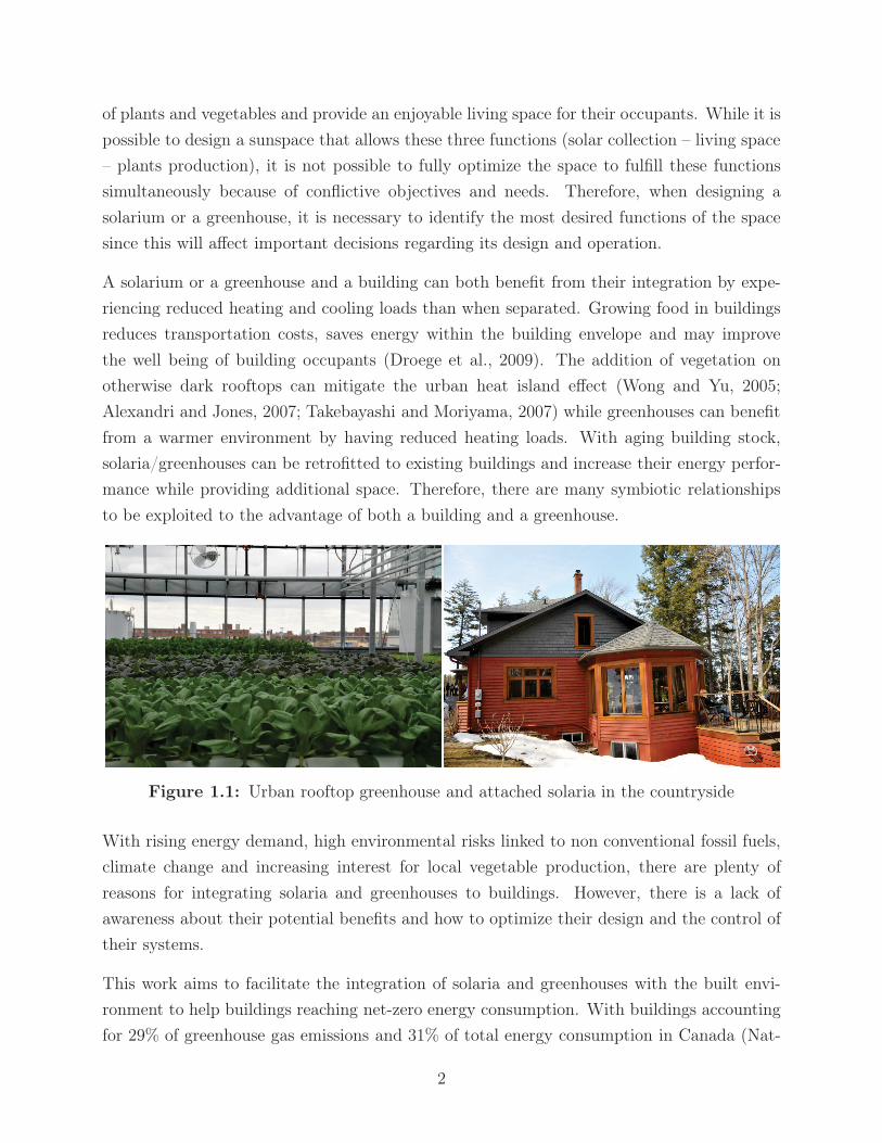
A solarium or a greenhouse and a building can both benefit from their integration by expe-

riencing reduced heating and cooling loads than when separated. Growing food in buildings

reduces transportation costs, saves energy within the building envelope and may improve

the well being of building occupants (Droege et al., 2009). The addition of vegetation on

otherwise dark rooftops can mitigate the urban heat island effect (Wong and Yu, 2005;

Alexandri and Jones, 2007; Takebayashi and Moriyama, 2007) while greenhouses can benefit

from a warmer environment by having reduced heating loads. With aging building stock,

solaria/greenhouses can be retrofitted to existing buildings and increase their energy perfor-

mance while providing additional space. Therefore, there are many symbiotic relationships

to be exploited to the advantage of both a building and a greenhouse.

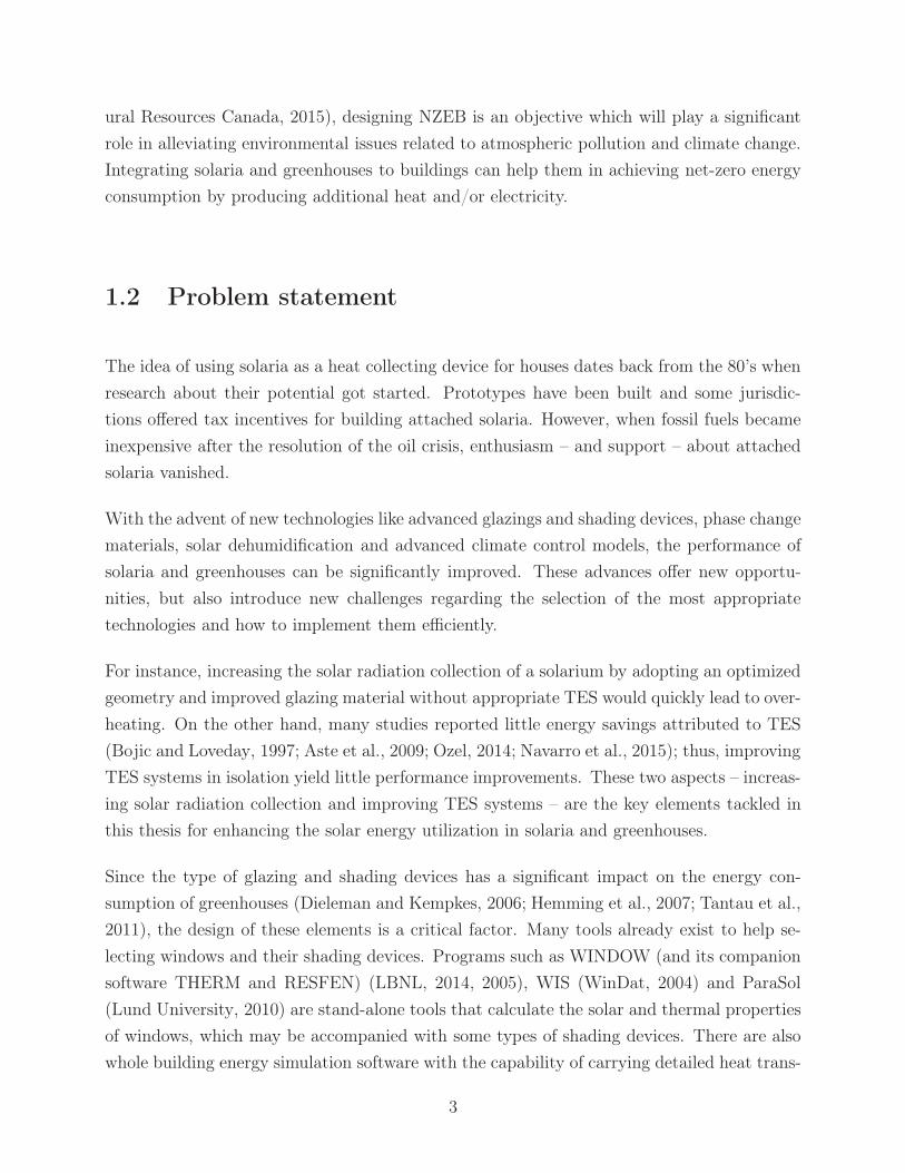
Figure 1.1: Urban rooftop greenhouse and attached solaria in the countryside

With rising energy demand, high environmental risks linked to non conventional fossil fuels,

climate change and increasing interest for local vegetable production, there are plenty of

reasons for integrating solaria and greenhouses to buildings. However, there is a lack of

awareness about their potential benefits and how to optimize their design and the control of

their systems.

This work aims to facilitate the integration of solaria and greenhouses with the built envi-

ronment to help buildings reaching net-zero energy consumption. With buildings accounting

for 29% of greenhouse gas emissions and 31% of total energy consumption in Canada (Nat-

2

ural Resources Canada, 2015), designing NZEB is an objective which will play a significant

role in alleviating environmental issues related to atmospheric pollution and climate change.

Integrating solaria and greenhouses to buildings can help them in achieving net-zero energy

consumption by producing additional heat and/or electricity.

1.2 Problem statement

The idea of using solaria as a heat collecting device for houses dates back from the 80’s when

research about their potential got started. Prototypes have been built and some jurisdic-

tions offered tax incentives for building attached solaria. However, when fossil fuels became

inexpensive after the resolution of the oil crisis, enthusiasm – and support – about attached

solaria vanished.

With the advent of new technologies like advanced glazings and shading devices, phase change

materials, solar dehumidification and advanced climate control models, the performance of

solaria and greenhouses can be significantly improved. These advances offer new opportu-

nities, but also introduce new challenges regarding the selection of the most appropriate

technologies and how to implement them efficiently.

For instance, increasing the solar radiation collection of a solarium by adopting an optimized

geometry and improved glazing material without appropriate TES would quickly lead to over-

heating. On the other hand, many studies reported little energy savings attributed to TES

(Bojic and Loveday, 1997; Aste et al., 2009; Ozel, 2014; Navarro et al., 2015); thus, improving

TES systems in isolation yield little performance improvements. These two aspects – increas-

ing solar radiation collection and improving TES systems – are the key elements tackled in

this thesis for enhancing the solar energy utilization in solaria and greenhouses.

Since the type of glazing and shading devices has a significant impact on the energy con-

sumption of greenhouses (Dieleman and Kempkes, 2006; Hemming et al., 2007; Tantau et al.,

2011), the design of these elements is a critical factor. Many tools already exist to help se-

lecting windows and their shading devices. Programs such as WINDOW (and its companion

software THERM and RESFEN) (LBNL, 2014, 2005), WIS (WinDat, 2004) and ParaSol

(Lund University, 2010) are stand-alone tools that calculate the solar and thermal properties

of windows, which may be accompanied with some types of shading devices. There are also

whole building energy simulation software with the capability of carrying detailed heat trans-

3

fer calculations through windows and fenestration systems like EnergyPlus (U.S. Department

of Energy, 2013), TRNSYS (Klein and al., 2010) and ESP-r (ESR U, 2011).

After reviewing the existing tools, it was found that there is a need to develop a simple tool

to be used at the early design stages allowing the comparison of the net energy gains of

various fenestration systems, where the influence of the shades on the SHGC and U-value of

the fenestration system is accounted for in the energy balance.

In addition, the type of control of movable shading devices may significantly impact the in-

door conditions inside a greenhouse. While it is recognized that the use of multiple shades

is an efficient way for reducing heat losses in greenhouses (Tantau et al., 2011), there is a

need for a new control method to improve their performance. Calculating the heat transfer

through multiple-layers fenestration systems requires detailed models characterizing the con-

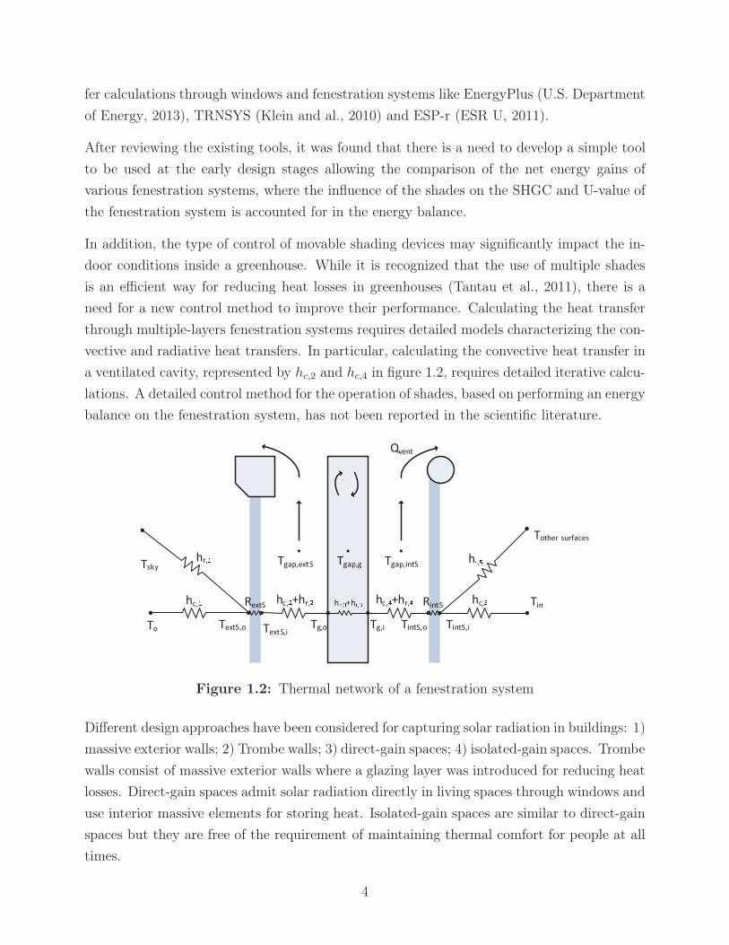
vective and radiative heat transfers. In particular, calculating the convective heat transfer in

a ventilated cavity, represented by hc,2 and hc,4 in figure 1.2, requires detailed iterative calcu-

lations. A detailed control method for the operation of shades, based on performing an energy

balance on the fenestration system, has not been reported in the scientific literature.

��

�������

����� ��������� ����

��������� ��������� ��������� ����

� �����

�

����� ������

����� �����

��� ���

������� �������������

����

��

Figure 1.2: Thermal network of a fenestration system

Different design approaches have been considered for capturing solar radiation in buildings: 1)

massive exterior walls; 2) Trombe walls; 3) direct-gain spaces; 4) isolated-gain spaces. Trombe

walls consist of massive exterior walls where a glazing layer was introduced for reducing heat

losses. Direct-gain spaces admit solar radiation directly in living spaces through windows and

use interior massive elements for storing heat. Isolated-gain spaces are similar to direct-gain

spaces but they are free of the requirement of maintaining thermal comfort for people at all

times.

4

TES systems are included in buildings to answer various needs, such as reducing energy

consumption, temperature fluctuations and delaying effects from peak solar gains. While

recommendations have been provided to meet some design targets for some applications, for

instances for reducing temperature fluctuations in direct-gain spaces, a systematic review

of the possible design targets along with appropriate design metrics to analyze them is still

lacking. In addition, a methodology and design recommendations for sizing TES systems

specifically for isolated-gain applications such as solaria and greenhouses are needed.

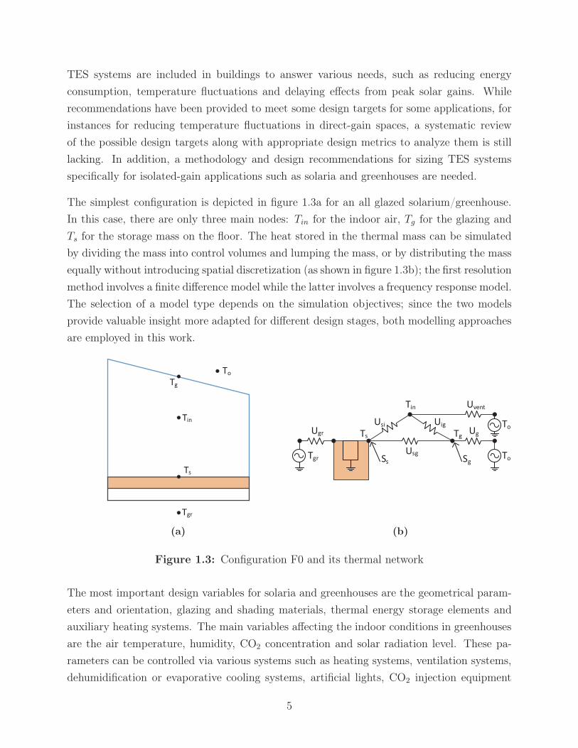
The simplest configuration is depicted in figure 1.3a for an all glazed solarium/greenhouse.

In this case, there are only three main nodes: Tin for the indoor air, Tg for the glazing and

Ts for the storage mass on the floor. The heat stored in the thermal mass can be simulated

by dividing the mass into control volumes and lumping the mass, or by distributing the mass

equally without introducing spatial discretization (as shown in figure 1.3b); the first resolution

method involves a finite difference model while the latter involves a frequency response model.

The selection of a model type depends on the simulation objectives; since the two models

provide valuable insight more adapted for different design stages, both modelling approaches

are employed in this work.

��

���

���

��

��

���

���

���

���

��� ���

��

��

���

�� ��

�� ��

��

(a) (b)

Figure 1.3: Configuration F0 and its thermal network

The most important design variables for solaria and greenhouses are the geometrical param-

eters and orientation, glazing and shading materials, thermal energy storage elements and

auxiliary heating systems. The main variables affecting the indoor conditions in greenhouses

are the air temperature, humidity, CO2 concentration and solar radiation level. These pa-

rameters can be controlled via various systems such as heating systems, ventilation systems,

dehumidification or evaporative cooling systems, artificial lights, CO2 injection equipment

5

and thermal/solar screens. The state of these variables will determine crop yields, energy

consumption and thermal comfort. The modification of one system element often impacts

more than one variable and sometimes, modifying a system will improve some variables while

adversely affecting others. It it thus necessary to have a global understanding of the various

physical processes occurring in solaria and greenhouses.

1.3 Scope of thesis

This work aims to improve the performance of solaria and greenhouses by enhancing their

solar energy utilization. This is best seen as a two fold process: solar radiation collection

should be first maximized and then used efficiently, where TES should be used for improving

the thermal conditions in the space. This thesis is focused on the design and control of

glazing and shading materials along with passive TES systems. Considerations related to

the integration of solaria and greenhouses in buildings are also discussed in this work, where

there are many symbiotic relationships that can be optimized to the advantage of both a

building and a greenhouse.

This thesis is providing guidelines to assist in the design and operation of energy efficient

solaria/greenhouses. These spaces can be versatile and support different functions. Possible

design targets are reviewed and suggestions for reaching them are provided. Solaria and

greenhouses can be supplemented with auxiliary heat or be designed to provide satisfactorily

interior conditions without any external heat; they can even collect surplus heat that can be

supplied to adjacent buildings and thus become net energy providers. Conventional solaria

and greenhouses, with their low insulation levels, require large amount of energy to maintain

comfortable conditions. However, with careful design and efficient operation, these spaces

can be converted from energy consumers to net energy providers. Indeed, the amount of

solar energy received by a greenhouse exceeds by far its annual energy needs, even in a cold

country like Canada.

This thesis is focused on designing solaria and greenhouses in cold climates like Canada and

northern Europe and Asia. Cold climates are defined by Hutcheon and Handegord (1995) as

locations having a winter design temperature of -7 °C or lower. Many recommendations are

also applicable – and desirable – in more favorable climates with less severe winters. However,

greenhouses in tropical climates are used for different reasons, like controlling water flows and

pest management, and therefore are outside the scope of this thesis.

6

The aim of this work is to develop methodologies and control strategies to assist building

designers for the design and control of solaria and greenhouses. Aspects specific to building-

integrated solaria and greenhouses are widely discussed in this work. To be fully integrated,

one must carefully consider and balance architectural, thermal, moisture and indoor air

quality issues with occupant needs. Both residential and commercial scale greenhouses have

a lot of potential in terms of heat and food production. With accelerated urbanization and

pressing environmental issues, this work presents a lot of potential to help cities all around

the world to be literally greener, more energy efficient and more sustainable while facilitating

access to fresh vegetables.

1.4 Thesis overview

This introduction is followed by a broad literature review on important design and control

considerations related to solaria and greenhouses. The first section is focused on the most

important design variables affecting the interior conditions: the geometrical parameters and

orientation, glazing and shading materials, TES systems and auxiliary heating systems. The

second section reviews strategies for the control of the main variables governing the indoor

climate: the indoor air temperature, relative humidity, solar radiation intensity and CO2

concentration. A selection of greenhouse climate control models is also presented, and the

concepts of closed and semi-closed greenhouses and their particular operational characteristics

are introduced. The third section focuses on building-integrated solaria and greenhouses.

Based on this review of the scientific literature, knowledge gaps and research opportunities

are identified in the last section.

Chapter 3 presents a short study on the energy saving potential of building-integrated so-

laria and greenhouses. Chapter 5, 6 and 7 are using different solarium models, which varies

depending on their objectives; some key common elements of the solarium models used in

these chapters are presented in chapter 4. Chapter 5 presents a methodology for the design

of fenestration systems, which calculates the annual performance of windows or glazings with

one interior shade, one exterior shade or the combination of both. A control algorithm for

improving the performance of these shading elements is presented in chapter 6. Finally, chap-

ter 7 presents frequency domain and finite difference models for the design of TES systems

in solaria and greenhouses and proposes a methodology along with design recommendations.

The conclusion presented in chapter 8 summarizes the main contributions of this work and

provides recommendations for future research in this field.

7

Appendix A presents tables for estimating the solar transmittance and absorptance of glass

panes from the U-value, SHGC and gas infill of an insulated glazing unit (IGU). They can be

used if this information is not available for the IGU of interest, when comparing various fen-

estrations systems with the methodology presented in chapter 5. The uncertainty associated

with the calculation of the heat stored and released by the PCM material in the experiment

presented in chapter 5 is presented in appendix B. Fundamental commonly used equations

employed in the models developed in this thesis are presented in appendix C, where equations

for modelling solar radiation availability and view factors are provided. Appendix D presents

the thermal networks and associated energy balance equations of five solaria/greenhouses

configurations, which can be used when implementing the methodology for sizing TES sys-

tems presented in chapter 7. The impact of varying glazing type and enhancing thermal

coupling on the main performance parameters have been analyzed with FR models and are

shown in appendix E. Detailed monthly results obtained with FD models are presented in

appendix F. Finally, appendix G shows a table for estimating the absorbed beam radiation

fraction by indoor surfaces for a latitude of 55°.

8

Chapter 2

Literature review

In desiring, through you, to point out to the London Horticultural Society, what the figure

is, which will receive the greatest possible quantity of the sun’s rays, at all times of the day,

and at all seasons of the year, I do not presume that any of the members are ignorant of the

solution of so simple a problem. [...] It must have occurred to you, that that form is to be

found in the sphere [...].

Mackenzie (1815)

This chapter presents an overview of the scientific literature on important design and control

considerations related to solaria and greenhouses. The first section discusses design elements

that play an important role in the performance of solaria/greenhouses, such as geometrical

parameters, glazing and shading materials and thermal energy storage systems. The second

section covers important aspects related to the control of different systems and their impact

on the main variables governing the indoor climate in greenhouses: the air temperature,

relative humidity, CO2 concentration and solar radiation level. The third section focuses

on issues and opportunities of fully integrating solaria and greenhouses with buildings. The

fourth and last section presents a succinct summary of the most relevant work and identify

research opportunities.

9

2.1 Designing low energy solaria/greenhouses

2.1.1 Geometrical parameters and orientation

The geometry and orientation of a greenhouse exert a significant effect on the indoor condi-

tions. The positioning of transparent and opaque surfaces as well as ventilation openings are

important design elements that must be carefully designed. This section presents a summary

of relevant studies conducted on these topics.

2.1.1.1 Solar radiation collection

Studies have been conducted as early as in the 19th century about the ideal shape a green-

house (so-called a forcing-house or hothouse at that time) should have to receive the greatest

quantity of solar radiation. In 1808, as mentioned by Knight (1808), it was known that the

maximum solar transmission through glass occurs when the sun’s ray fall most perpendicu-

larly on it. From his experiments, he suggested to select a south-facing roof with an elevation

of 34° under his latitude of 52°.

Reverend Wilkinson published in 1809 a rule generalizing how to determinate the best roof

angle of a glass house for all climates:

«Having determined in what season, we wish to have the most powerful effects from the sun, we

may construct our houses accordingly by the following rule. Make the angle contained between the

back wall of the house and its roof, = to the complement of the latitude of the place, ± the sun’s

declination for that day on which we wish his rays to fall perpendicularly. From the vernal to the

autumnal equinox, the declination is to be added, and the contrary.» Wilkinson (1809)

Mackenzie (1815) suggested a spherical shape for greenhouses as being the shape receiving

the greatest quantity of rays from the sun. However, Loudon (1817) tempered his enthusiasm

by noting that while it is true that the center of a sphere receives the maximum rays, points at

different locations, such as the back wall or the floor, receive less radiation and such a shape

induces a lack of solar radiation uniformity impinging on the crop. In addition, it was observed

that young leafs were burned in spherical greenhouses due the the concavity of the glass

which focused light, and that ventilation openings were insufficient – due the curvilinearity

of the structure which prevents operable sashes – which caused excessive humidity (Taylor,

1995).

10

Many studies have analyzed the effect of the orientation on different greenhouse shapes

in various locations. Studies conducted in England (Lawrence, 1963; Harnett, 1975), Japan

(Kozai, 1977b), Italy (Facchini et al., 1983), Portugal (Rosa et al., 1989) and India (Gupta and

Chandra, 2002) suggested/concluded that it is beneficial for greenhouses to have their longest

side facing south. Harnett (1975) measured 7.4%-10.5% higher solar radiation transmission

throughout the year in a east-west greenhouse compared to the same north-south oriented

greenhouse, located in England. Sethi (2009) concluded that an east-west orientation should

be preferred at all latitudes except near the equator because a greenhouse with this orientation

receives more radiation in winter, when it is most needed.

These conclusions are consistent with passive solar design principles, which identified south

façades as the most useful orientation for maximizing solar radiation transmission in winter

and limiting solar penetration in summer (Butti and Perlin, 1980; Parekh et al., 1990).

An aspect ratio (the length of a building divided by its width) of 1.2 to 1.3 is often rec-

ommended for passive solar houses (Athienitis, 2007; CMHC, 1998). However, such rules of

thumb are nor reported for greenhouses.

Kozai (1977b) carried simulations of single span greenhouses with different roof angles (16°,

32°, 52°) and orientations at three different latitudes. It was found that the transmissivity

(i.e. the ratio of solar radiation falling onto the greenhouse glazing to the radiation falling on

a horizontal plane in the greenhouse) of a east-west greenhouse in Amsterdam (latitude of

52°), Sapporo (43°) and Tokyo (35°) is higher with a roof angle of 52° at the winter solstice.

However, the difference between 52° and 32° is very small for the three cities.

Kozai (1977a) also conducted simulations of multispan greenhouses of infinite length and no

structural members with a ratio of the height of the side walls to the width of one span of

0.8 (roof angle of 20°). He found that the transmissivity of a north-south greenhouse was

barely affected by the number of span while a est-west greenhouse is significantly affected.

In Osaka, (latitude of 34°), the average transmissivity of a span is about 90% for the first

two spans but it decreases smoothly to reach a constant transmissivity of about 75% from

spans 5-8 (at winter solstice). However, for Amsterdam, the average transmissivity remains

at about 90% for the first fourth spans but keeps decreasing until reaching about 65% at the

eighth span.

Kumar et al. (1994) reported that for the same glass area, the south glass oriented at the

optimum angle for a given latitude gives better thermal comfort compared to a vertical south

glass or a combination of vertical and tilted glass.

11

Some studies found that having a reflective north wall in east-west oriented greenhouses sig-

nificantly increases their transmissivity. Thomas (1978) reported that a back wall inclined

at 75° increases the transmissivity the most. In addition, they noted that having a reflec-

tive north wall brings the opportunity to insulate that wall, therefore reducing heat losses.

Lawand et al. (1975) judiciously noted that having a reflective north wall slope approximately

equal to the maximum solar altitude at the summer solstice is ideal. Indeed, having a higher

slope would not significantly enhance the amount of light reflected on the plants while having

a smaller slope would decrease the amount of transmitted light in summer.

Critten (1983) conducted simulations and found that an infinitely long multispan greenhouse

with a roof slope of 56° has an average transmissivity 3% higer than with a roof slope of

26° (at a latitude of 52°). He also conducted simulations of different greenhouse designs

with symmetrical and vertical south roofs under diffuse and direct light (Critten, 1984).

He found that under some circumstances, a double glazed greenhouse with a vertical south

roof may have an 8% increase in transmissivity compared to a single glazed symmetrical

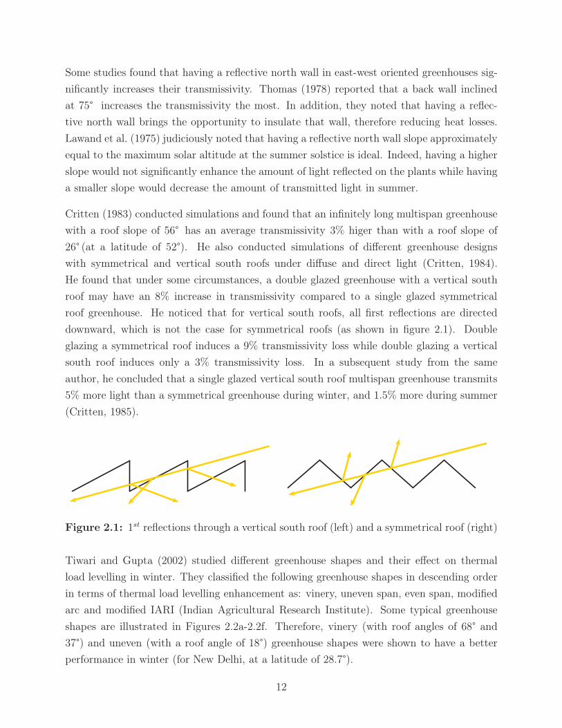
roof greenhouse. He noticed that for vertical south roofs, all first reflections are directed

downward, which is not the case for symmetrical roofs (as shown in figure 2.1). Double

glazing a symmetrical roof induces a 9% transmissivity loss while double glazing a vertical

south roof induces only a 3% transmissivity loss. In a subsequent study from the same

author, he concluded that a single glazed vertical south roof multispan greenhouse transmits

5% more light than a symmetrical greenhouse during winter, and 1.5% more during summer

(Critten, 1985).

Figure 2.1: 1st reflections through a vertical south roof (left) and a symmetrical roof (right)

Tiwari and Gupta (2002) studied different greenhouse shapes and their effect on thermal

load levelling in winter. They classified the following greenhouse shapes in descending order

in terms of thermal load levelling enhancement as: vinery, uneven span, even span, modified

arc and modified IARI (Indian Agricultural Research Institute). Some typical greenhouse

shapes are illustrated in Figures 2.2a-2.2f. Therefore, vinery (with roof angles of 68° and

37°) and uneven (with a roof angle of 18°) greenhouse shapes were shown to have a better

performance in winter (for New Delhi, at a latitude of 28.7°).

12

(a) Gable or evenspan greenhouse (b) Uneven greenhouse

(c) Quonset greenhouse (d) Vinery greenhouse

(e) Gothic arch greenhouse (f) Modified arch greenhouse

Figure 2.2: Common greenhouse shapes

In another study, Gupta and Chandra (2002) analyzed three different shapes of greenhouses in

their simulations: quonset, gable and gothic arch. They found that a gothic arch greenhouse

consumed 2.6% and 4.2% less heat than a gable and quonset greenhouse, respectively (located

in northern India, latitude of 28.3°). Gupta (2004) also analyzed the effect of different

greenhouse shapes on the weighted solar fraction of the north partition wall. Their results

showed that the weighted solar fraction was higher for an even span shape than for uneven

shape at latitudes of 13°-34°. However, although of some interest, the weighted solar fraction

of the north wall is not the most appropriate variable to optimize; solar radiation incident

on the floor is as useful as the radiation incident on the wall, contributing to photosynthesis

when absorbed by plants and thermal load levelling when absorbed by the floor.

Malquori et al. (1993) have studied different single-span greenhouse shapes (oriented east-

west) and found that a greenhouse with an asymmetrical profile with a south roof slope of

13

29° and a north roof slope of 34° could collect more solar radiation than the other greenhouse

profiles studied (at a latitude of 43.5°).

Soriano et al. (2004) studied solar radiation transmission with scale greenhouse models in

Granada, Spain (latitude of 37°). Their results for three spans greenhouses are summarized

in Table 2.1. It can be seen that the greenhouse scale model with a symmetrical roof angle of

27° has the highest solar radiation transmission in winter while the greenhouse with a south

roof angle of 18° and a north roof angle of 8° has a higher transmission at the equinox and

in summer.

Roof angle (°) Seasonal transmissionSouth slope North slope Summer solstice Equinox Winter solstice

18 8 74.9 69.8 59.036 55 69.7 66.3 56.745 27 71.3 67.7 66.627 27 71.0 68.5 70.1

Table 2.1: Mean seasonal transmission for four scale models with different roof slopes (fromSoriano et al. (2004))

Beshada and Zhang (2006) conducted simulations of a solar greenhouse design developed in

northern China adapted to the winter conditions in Manitoba. As illustrated in figure 2.3,

this type of greenhouse has an insulated north wall and roof as well as side walls. The back

wall is filled with sand and a thermal blanket is manually unrolled at night. Their study

pointed out that the slope of the north roof must be higher that 46°-60° at latitudes of 58°-

43° to avoid shading of the north wall (by the north roof) until the end of April. Shading

during summer might be considered as an asset to reduce ventilation loads. Simulations

conducted for a latitude of 49° indicated that up to 35% of the north wall might be shaded

by end walls in December for a 30 m long greenhouse (with an aspect ratio of 4.3). It is

therefore suggested that greenhouses with insulated side walls should be as long as possible

to reduce this effect.

Lawand et al. (1975) at the Brace Research Institute carried out simulations and experimen-

tations of greenhouses in Québec and proposed a new design to improve the performance in

winter by having a transparent sloped south roof and vertical walls with a reflective (and

insulated) north wall (see figure 2.4). From simulations, they concluded that the range of val-

ues of tilt angles for near optimum design is 40-70° for the south wall and 60-75° for the north

wall. By analyzing data obtained for a prototype greenhouse, they estimated that this green-

14

Figure 2.3: A typical chinese solar greenhouse

Figure 2.4: A greenhouse design developed by the Brace Research Institute

house design can lead to a 30%-40% reduction of heating requirements when compared with

the most common greenhouse type (quonset shape with double polyethylene cover).

While many studies have been conducted for various types of greenhouses in different climates,

some authors have noted the lack of general guidelines for optimal roof slopes (Soriano et al.,

2004) and the need for a model to compare various design options (Gupta and Chandra,

2002).

15

2.1.1.2 Natural ventilation

Natural ventilation (and infiltration) in buildings is driven by pressure differences induced

by wind and air density differences between indoor and outdoor (buoyancy, or stack effect)

(ASHRAE, 2009, chapter 16). However, during warm weather, the stack effect is limited

and natural ventilation depends mainly on wind forces (Bot, 1983; Zemanchik et al., 1991).

Boulard and Baille (1995, Fig. 9) have shown, for a specific case, that at wind speeds of 0.5-

0.7 m/s, the buoyancy and wind speed driven ventilation have about the same magnitude,

but that ventilation due to wind is more than 8 times greater than buoyancy effects at a wind

speed of 2 m/s. Hellickson and Walker (1983) suggested to orient the length of a building

(and ventilation inlets) perpendicular to the prevailing winds to enhance natural ventilation.

They also noted that it is not unusual to have prevailing winds with different directions in

summer and in winter.

However, the impact of a building orientation on the natural ventilation flow may be not

very significant. A study found that the average ventilation rate for a naturally vented

building for the best orientation is only 13% higher than for the worst orientation (at outdoor

temperatures above 20°C) (Zemanchik et al., 1991).

Ventilation flux in naturally vented greenhouses have been simulated using various theoretical

and Computational Fluid Dynamics (CFD) models (Boulard and Baille, 1995; Seginer, 1997;

Mistriotis et al., 1997; Boulard et al., 1999; Lee et al., 2005; Ould Khaoua et al., 2006).

However, the ventilation rate depends strongly on greenhouses design characteristics like

the aspect ratio and position of openings, as well as on the wind direction and intensity.

Therefore, the conclusions of studies are applicable only for the specific cases investigated;

generalizations are not possible (Mistriotis et al., 1997). Because of the difficulties to identify

general guidelines for optimum greenhouse design for natural ventilation, this field of study

is still under active development.

Greenhouses typically have ventilation openings along the longest side at the roof ridge

and/or along a side wall (see figure 2.5). Bot (1983) estimated that the addition of side vents

on only 10% of the side wall of a greenhouse equipped with roof vents only may increase the

ventilation rate by almost 70%.

Lee et al. (2000) have shown with 2D CFD simulations that having side vents openings

closer to the ground increases natural ventilation rates for a double polyethylene multi-span

greenhouse. It also favors ventilation efficiency by reducing short-circuiting, i.e. air incoming

by the side vents and exiting directly through the 1st roof vent without mixing. They also

16

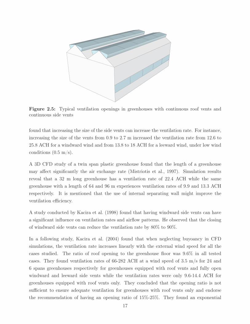
Figure 2.5: Typical ventilation openings in greenhouses with continuous roof vents andcontinuous side vents

found that increasing the size of the side vents can increase the ventilation rate. For instance,

increasing the size of the vents from 0.9 to 2.7 m increased the ventilation rate from 12.6 to

25.8 ACH for a windward wind and from 13.8 to 18 ACH for a leeward wind, under low wind

conditions (0.5 m/s).

A 3D CFD study of a twin span plastic greenhouse found that the length of a greenhouse

may affect significantly the air exchange rate (Mistriotis et al., 1997). Simulation results

reveal that a 32 m long greenhouse has a ventilation rate of 22.4 ACH while the same

greenhouse with a length of 64 and 96 m experiences ventilation rates of 9.9 and 13.3 ACH

respectively. It is mentioned that the use of internal separating wall might improve the

ventilation efficiency.

A study conducted by Kacira et al. (1998) found that having windward side vents can have

a significant influence on ventilation rates and airflow patterns. He observed that the closing

of windward side vents can reduce the ventilation rate by 80% to 90%.

In a following study, Kacira et al. (2004) found that when neglecting buyoancy in CFD

simulations, the ventilation rate increases linearly with the external wind speed for all the

cases studied. The ratio of roof opening to the greenhouse floor was 9.6% in all tested

cases. They found ventilation rates of 66-282 ACH at a wind speed of 3.5 m/s for 24 and

6 spans greenhouses respectively for greenhouses equipped with roof vents and fully open

windward and leeward side vents while the ventilation rates were only 9.6-14.4 ACH for

greenhouses equipped with roof vents only. They concluded that the opening ratio is not

sufficient to ensure adequate ventilation for greenhouses with roof vents only and endorse

the recommendation of having an opening ratio of 15%-25%. They found an exponential

17

reduction of the ventilation rate with the number of spans being increased from 6 to 24

for greenhouses with roof and side vents, while the reduction was much less pronounced for

greenhouses with roof vents only.

He et al. (2015) conducted a 3D CFD study on an 11 span plastic greenhouse for analyzing

the effects of varying vents openings on the interior microclimate during the summer and

winter seasons. They recommend to use roof and side vents for summer cooling and roof

vents only for winter dehumidification. They reported that in winter, the use of roof and side

vents has the highest dehumidification potential, but also experiences the highest heat losses.

The use of side vents only offers the highest dehumidification efficiency, but also provides the

worst temperature and humidity homogeneity in the crop canopy, and thus suggest to use

roof vents only as a good compromise between heat losses, dehumidification efficiency and

microclimate homogeneity.

2.1.2 Glazing and shading materials

Many different materials can be used as greenhouse covers. Traditionally, clear glass was the

only material available, but plastic materials are now widely used. Plants need solar radiation

at wavelengths between 400-700 nm, which is the part of the spectrum typically called the

photosynthetically active radiation (PAR) (Mccree, 1971). In cold climates, it is desirable to

select materials with a high transmittance to short-wave solar radiation (0.2-3 μm) to reduce

heating needs. In addition, a good greenhouse cover would ideally have a low emissivity at

long-wave radiations (>3μm) and therefore a low thermal transmittance to reduce heat losses

during the cold season.

This section is divided into three sub-sections which describ different greenhouse cover types:

glass, rigid plastics and flexible plastic films. Typically, glass is the most durable and expen-

sive cover material while flexible films are the least expensive and durable materials. Whereas

increasing the insulation of greenhouse cover materials is indeed a good way to save energy, it

also increases the relative humidity level (Bailey, 1984), and therefore humidity management

becomes more important. These considerations are covered in details in section 2.2.2.

2.1.2.1 Glass

Glass is an excellent cover material that is durable, but heavy and expensive. In Germany,

90% of the total greenhouse floor area is covered by glass and 98.5% in the Netherlands, but

18

only 45%, 10% and 5% in France, Italy and Greece respectively (Briassoulis et al., 1997).

In Canada, 34% of greenhouse floor area is covered by glass, but only 28% and 13% in

the provinces of Ontario and Québec respectively (Statistics Canada, 2010). Typically, only

single glass was used for greenhouses, but with rising energy prices, double glass is now

sometimes being used in some countries like Germany, but still represents less than 5% of

glass covered greenhouse area (Briassoulis et al., 1997). Triple glass, which is heavy and

costly, is not being used in commercial greenhouses at the moment.

Table 2.2 on page 21 lists important parameters characterizing the performance of glass and

plastic covers. The typical clear glass presented in this table is representative of a typical

clear float glass. Low iron glass can increase the transmittance and eliminate the greenish

tint of normal clear glass. Anti reflective (AR) coatings can be applied on glass to reduce the

reflective component and increase the transmittance. By using these advanced technologies,

manufacturers can now produce glass with a visible transmittance as high as 0.993 and solar

transmittance up to 0.910 (LBNL, 2012). The three AR glass panes presented in table 2.2 are

the ones with the highest visible transmittance, the highest solar transmittance and the best

combination of high solar and visible transmittance available from the International Glazing

Database LBNL (2012).

Low emissivity (low-e) coatings can be applied to glass to reduce radiative heat losses. These

coatings can be divided into two categories: hard coatings and soft coatings. Hard coat-

ings are based on tin oxide and use a pyrolytic process which creates a hard, durable coat.

Soft coatings are usually produced in a sputtered process and have a soft finish which must

be protected (Hammarberg, 2003). Only hard coatings can be used on single windows be-

cause soft coatings have to be applied on surfaces #2 or #31 of insulated glass units for

longevity. Typically, hard low-e have a higher solar transmittance and higher emittance that

soft low-e.

While the presence of a low-e coating increases the thermal resistance of a window, it also

reduces its light and solar transmittance. However, applying an AR coating could reduce this

effect (Rosencrantz et al., 2005). The hard low-e glass listed in table 2.2 is a typical clear

glass with a pyrolytic coating. The hard low-e AR glass below is the pyrolytic low e glass

with the highest visible and solar transmittance available on the market. From table 2.2, it

can be seen that AR low-e single glass can offer almost the same visible transmittance as clear

glass while reducing its U-value by 38%, although at the expense of a solar transmittance

10% lower. The low-e coating is on the inner pane of the glass, which gives a lower U-value

1Surfaces are numbered from the exterior to the interior, with the exterior surface of the exterior glassbeing #1, the interior surface of the exterior glass being #2, etc.

19

than when deposited on the outer pane, but it also reduces the temperature of the inner

pane, which is even lower than for clear glass (Nijskens et al., 1984); therefore, if used in

greenhouses, good humidity management is needed to avoid condensation problems.

It is possible to combine two panes of glass into a sealed unit to create an insulated glass

unit (IGU). Inert gas like argon and even krypton can be used to fill the unit for reducing

convection in the glass cavity and further reduce the U-value. A selection of some of the best

IGU’s that can be created from the best window panes available on the market are listed in

table 2.2.

A study conducted in the Netherlands compared a conventional greenhouse with single glass

with different greenhouse covers: single AR glass, single AR low-e glass, double AR glass

and double AR low-e glass. They found that the four alternative greenhouse covers had a

higher economic yield, with the single and double AR glass being the most attractive option

for maximizing profit (Hemming et al., 2007).

2.1.2.2 Rigid plastics

Rigid plastics are used to cover 9% of the greenhouse area in Germany, 6% in France and less

than 3% in Italy, Greece and Netherlands (Briassoulis et al., 1997). In Canada and Ontario,

rigid plastics cover 7% of the total greenhouse floor area while this number rises to 9% for

Québec (Statistics Canada, 2010). Rigid plastics may be used on new greenhouses or for

retrofitting existing glasshouses. With their lower weight, it would be possible to remove

some structural members and therefore reduce structural shading (Giacomelli and Roberts,

1993).

Polycarbonate (PC) panels are available as single layer corrugated sheet and as double or

triple multilayered cross sections for improved strength and insulation. These panels are

affected by UV radiation and should be protected for durability (Giacomelli and Roberts,

1993).

Acrylic or polymethyl methacrylate (PMMA) is better known under its commercial name,

Plexiglass ®. It is available as flat or corrugated sheet and double multilayered cross sections.

Its transmittance is slightly lower than glass and is characterized by a high coefficient of

thermal expansion, so a careful installation is required (Papadakis et al., 2000). Acrylic

panels have potential fire problems (Giacomelli and Roberts, 1993).

20

Polyvinyl chloride (PVC) is found in the form of corrugated sheets. Its transmittance in the

PAR region is uneven: it is lower in the yellow band, but higher in the red and blue regions.

This material is not totally opaque to infrared radiation (Papadakis et al., 2000).

Fiberglass reinforced polyester (FRP) panels are manufactured as rigid corrugated sheets

with surface protection to reduce yellowing (like a thin Tedlar ® coating) (Papadakis et al.,

2000). Like acrylic, FRP panels have potential fire problems, but are resistant to hail dam-

age (Giacomelli and Roberts, 1993). FRP has the highest thermal transmittance from all

greenhouse covers (see table 2.2).

Material Transmittance U-valueSolar PAR Long wave (W/m2K)

Single glassTypical clear glass 84.1 89.9 5.92AR glass 1 84.3 99.3 5.97AR glass 2 91.0 91.6 5.92AR glass 3 88.1 97.3 5.97Glass - hard low-e 63.5 82.0 3.61Glass - hard low-e - AR 74.8 88.8 3.68Double glassTypical clear/x2 - Air 71.6 81.3 2.73AR glass 3 /x2 - Argon 79.8 94.7 2.63Typical clear/Typical low-e - Argon 63.0 76.4 1.65AR glass 3/hard low-e - Argon 68.0 86.5 1.62Hard low-e - AR/x2 - Argon 59.9 79.5 1.29Rigid plastic Single/Double

Polycarbonate (PC) 77 78 3 /3.2-3.5PMMA 82 86 1 /3.0-3.4Rigid PVC 81 84 6 6.6/3.3Fiberglass (FRP) 75-87 - 87-90Plastic filmsLDPE 88-89 63-65 9.0/6.4PE-IR 85-86 12-28PVC 85-90 10-15 7.6/EVA 90 13-25 7.8/ETFE Cascone et al. (2005) 93-95 22-29

Table 2.2: Important parameters for most common greenhouse coverings. Values for glasswere selected from the library in Windows LBNL (2012) and optical values for rigid andflexible plastic covers are taken from Papadakis et al. (2000), unless specified otherwise.U-values of plastics materials are taken from Nijskens et al. (1984).

21

2.1.2.3 Plastic films

Plastic films are widely used in warm european countries: they cover 94% of greenhouse area

in Greece, 87% in Italy and 49% in France, but only 1% in Germany and the Netherlands

(Briassoulis et al., 1997). However, in Canada, Ontario and Québec, as much as 60%, 65% and

78% of greenhouse area is covered by plastic film respectively (Statistics Canada, 2010).

Polyethylene (PE) film is the most common greenhouse cover in the United-States. They have

a lifetime of 2-4 years before being degraded by UV radiations. Low-density polyethyelene

(LDPE) has a relatively high solar transmittance and but also the highest thermal trans-

mittance of all cover materials (see table 2.2). It is possible to add additives to PE films to

reduce thermal transmittance (Giacomelli and Roberts, 1993). These thermal polyethylene

films (PE-IR) can bring the thermal transmittance of about 0.65 as low as 0.12 with only a

small reduction of solar transmittance.

Polyvinyl chloride (PVC) films are used extensively in Japan, but their use is limited in

Europe. They exhibit a high solar transmittance and a low thermal transmittance. How-

ever, their higher cost compared to PE limit their integration as well as the harmful dioxin

emissions that are released when burned (Papadakis et al., 2000).

Ethylene vinyl acetate copolymer (EVA) is produced by the co-polymerization of ethylene

with vinyl acetate, which reduces the thermal transmittance (Papadakis et al., 2000). It has

a high solar transmittance and a relatively low thermal transmittance.

A study found that Ethylene-tetra-fluorine-ethylene ETFE has a significantly higher solar

transmittance and lower thermal transmittance than PE and EVA, resulting in a higher

mean air temperature inside a greenhouse (Cascone et al., 2005). ETFE is a very promising

material, however its high cost limits its integration (Bot et al., 2005). The installation of

this material is often carried out in multiple layers in combination with forced ventilation

in the cavities. Such an installation requires particular care and regular maintenance to

ensure the performance and air tightness of the structure is thus less adapted to small scale

facilities.

Air born exposure of Bisphenol A (BPA) can occur by off-gassing of plastic products. BPA is

considered as an endocrine disrupting compound which can cause adverse health effect, even

at low doses. BPA is part of polycarbonate plastics and often used as an additive to other

plastics such as PVC. Phthalates are also commonly used as plasticizers to impart flexibility

and elasticity to polymers such as PVC. They are not monomers as BPA and are therefore

more prone to leaching out of products. Phthalates can compose a major part of plastics,

22

sometimes up to 80% by weight. They are endocrine disrupting compounds with suspected

health effects on reproductive systems. Both BPA and phthalates are commonly found in

humans and even in breast milk. Other additives to plastics are also a source of concerns,

like polyhalogenated flame retardants (Halden, 2010).

2.1.2.4 Shading systems

Shades can be used in greenhouses to reduce solar gains and heat losses. A shade whose main

purpose is to reject near infra-red radiation (NIR) is called a solar screen while a shade whose

main purpose is to allow solar heat and reduce heat losses is named a thermal screen. For

both types of shades, visible and PAR radiation should not be blocked to provide daylight to

occupants and plants. The ideal solar screen should therefore reject the near-infrad portion

of the solar spectrum rather than the visible part. Reflection of the NIR region is preferred to

absorption to reduce solar heat gains. Having a low transmittance at far-infrared wavelengths

would be beneficial to reduce night heat losses (Nijskens et al., 1985).

While rejecting NIR is beneficial in summer for reducing the air temperature inside green-

houses, allowing NIR is useful for supplying heat in winter (Kempkes, 2008). Therefore, an

ideal shade for the winter season would have a high solar and visible transmittance but a low

thermal transmittance.

A third type of screen can also be used: a blackout screen, to be used only at night. Its ther-

mal properties are optimized to reduce heat losses only without considering solar properties

(Meyer, 2011).

The possibilities of using up to three screens is now envisioned to reduce the energy con-

sumption of greenhouses. One shade would be a solar screen, aluminised and NIR reflective;

another one would be a thermal screen, with a high PAR and solar transmittance; the third

one would be a black-out screen, which should have a low U-value. Combining three screens

could lead to a reduction of energy consumption of 80% (Tantau et al., 2011).

There are many different shades with different properties available on the market. Important

properties of common screen materials and methods for determining screens properties can

be found in Roberts et al. (1981), Nijskens et al. (1985) and Cohen and Fuchs (1999). Control

strategies for the opening and closing of shades are presented in section 2.2.1.3.

23

2.1.2.5 Design tools for the selection of glazing and shading materials

The selection of the optimum glazing for a house or a greenhouse is a tedious task. This

section discusses issues related to the design of glazing and shading elements and presents

some existing tools that can be used to assist in this task. These tools have been designed

primarily for the design of residential and office buildings, but could be helpful for designing

solaria and greenhouses as well.

Selecting the best windows for a house is more complicated than selecting the best walls,

since the performance of windows is governed by two major variables: the solar heat gain

coefficient (SHGC) and the thermal resistance. In cold climates, it is desirable to have

windows with both high thermal resistance and SHGC. However, these two variables usually

move in opposite directions: as the thermal resistance increases, usually the SHGC decreases.

In addition, windows are one the most expensive component in a house (on a unit area basis).

As a result, the selection of windows is one of the the most problematic aspect of net-zero

energy buildings (NZEB) (Proskiw, 2010).

Furthermore, the use of shading devices (and their operation if moveable) significantly affect

the performance of windows by altering their thermal resistance and solar gains. Some tools

are available to guide designers for selecting windows. RESFEN 5.0 (LBNL, 2005) calculates

the heating and cooling energy use associated with windows. It also calculates cost associated

with energy use and peak heating and cooling demand. RESFEN, developed by the Lawrence

Berkeley National Laboratory, comes with a rather limited default set of window library, but

data for other windows can be easily imported from WINDOW 6.3 (LBNL, 2014). Windows

can be oriented north, east, south and west and skylights can also be simulated. However,

other orientations cannot be selected. Some types of fixed shading devices, like overhangs,

interior shades, exterior obstructions or a combination of these can be simulated. However,

their shading capability is constant and cannot be modified nor controlled.

ParaSol (Lund University, 2010) is mainly used for the design of solar protection on windows

at an early design stage. Interior, exterior and between the panes shades can be simulated

simultaneously. Awnings, venetian blinds, brises-soleil, roller shades, shutters and pleated

curtain can be simulated, but side fins are still not available. Default shades and windows

are available in a library and it is also possible to specify custom shades and windows. Only

one orientation is simulated at each run, but any orientation can be selected. The monthly

solar and visible transmittance of the bare window and the window-shade system are given

as outputs. It is possible to define simple controls of sunshades, based on solar radiation

intensity, indoor/outdoor temperatures or a hourly schedule. Results from energy balance

24

calculations are the peak heating and cooling loads and annual heating and cooling demands

with and without sunshades. This tool is useful for designing solar protection and visualizing

its effects versus a bare window, but cannot be used to compare the performance of various

windows and shades combinations for the design stage.

WIS (WinDat, 2004) is a European tool for calculating optical and thermal properties of

windows and shading systems. The development of the standard ISO 15099 (2003) for calcu-

lating the thermal performance of windows was inspired by this software for calculating the

solar optical properties of shading devices (Tzempelikos, 2008).

RESFEN, WINDOW, WIS and ParaSol are stand-alone tools that calculate the solar and

thermal properties of windows, which may be accompanied with some types of shading de-

vices. WINDOW and WIS are mainly used for certification purposes as they carry out

simulations at fixed conditions, usually chosen to match a specific standard. RESFEN and

ParaSol offer the possibility of calculating annual heating and cooling loads associated with

windows. There are also whole building energy simulation software with the capability of

carrying detailed heat transfer calculations through windows and fenestration systems like

EnergyPlus (U.S. Department of Energy, 2013), TRNSYS (Klein and al., 2010) and ESP-r

(ESR U, 2011). A more detailed description of these software can be found in Loutzenhiser

et al. (2007), Tzempelikos (2008) and in Rogalsky (2011).

Nielsen et al. (2001) presented a simple method for comparing the energy performance of

glazings or windows for heating dominated buildings. The net energy gain is calculated for

the heating season and is equal to the solar gains minus the heat losses through the glazing.

Following this method, diagrams presenting the net energy gain for different combinations of

SHGC and U-values are generated for a specific orientation. Such diagrams allow a designer

to quickly visualize what is the best window for a given orientation, which is needed at the

design stage. Heat gains can be reduced by employing a shading coefficient to represent

overhangs or obstructions, but only a fixed value for the year can be simulated and the

thermal effects of including different shading devices are not accounted for.

Upon review of the existing tools, it is observed that none has been designed to perform

comparisons of different window/shade systems specifically for the design stage. There is

a need to develop a tool allowing the visualization of the energy performance of different

window/shade combinations that takes into account the effects of a shade on the overall

solar and thermal transmission of the fenestration system.

25

2.1.3 Thermal energy storage

Thermal energy storage (TES) is particularly needed for intermittent energy sources such

as solar energy. Diurnal storage accumulates heat during the day and releases it at night,

following a 24 hour cycle, while seasonal storage accumulates solar heat during summer

months to provide heating during winter months, following a yearly cycle (Hadorn, 2005).

Short term storage (less than a week) is the most common type. Abundant surplus heat is

available in the summer but seasonal storage is limited due to economic factors (Kaygusuz,

1999).

TES are usually classified by the process which is involved in storing heat: sensible heat

storage materials accumulate heat by changing temperature, latent heat storage materials

accumulate heat by changing phase (Kaygusuz, 1999) and thermochemical heat storage ma-

terials accumulate heat by physico-chemical process (like adsorption or absorption) (Hadorn,

2005).

Important criteria for TES materials are (Hadorn, 2005):

• Capacity and density

• Loading and unloading rate

• Efficiency of thermal storage (Eout/Ein)

• Stability (mechanical, chemical)

• Reversability during a number of cycles

• Cost

• Toxicity

• Recyclability assessed through a life cycle analysis

The following sub-sections present the most commonly used materials for TES, strategies for

sizing TES and examples of greenhouses with TES systems.

2.1.3.1 Materials

The most common type of thermal storage consists of sensible heat storage, where heat is

stored by raising the temperature of the storage medium. The heat stored in a medium can

be calculated from

Q = mcpΔT (2.1)

26

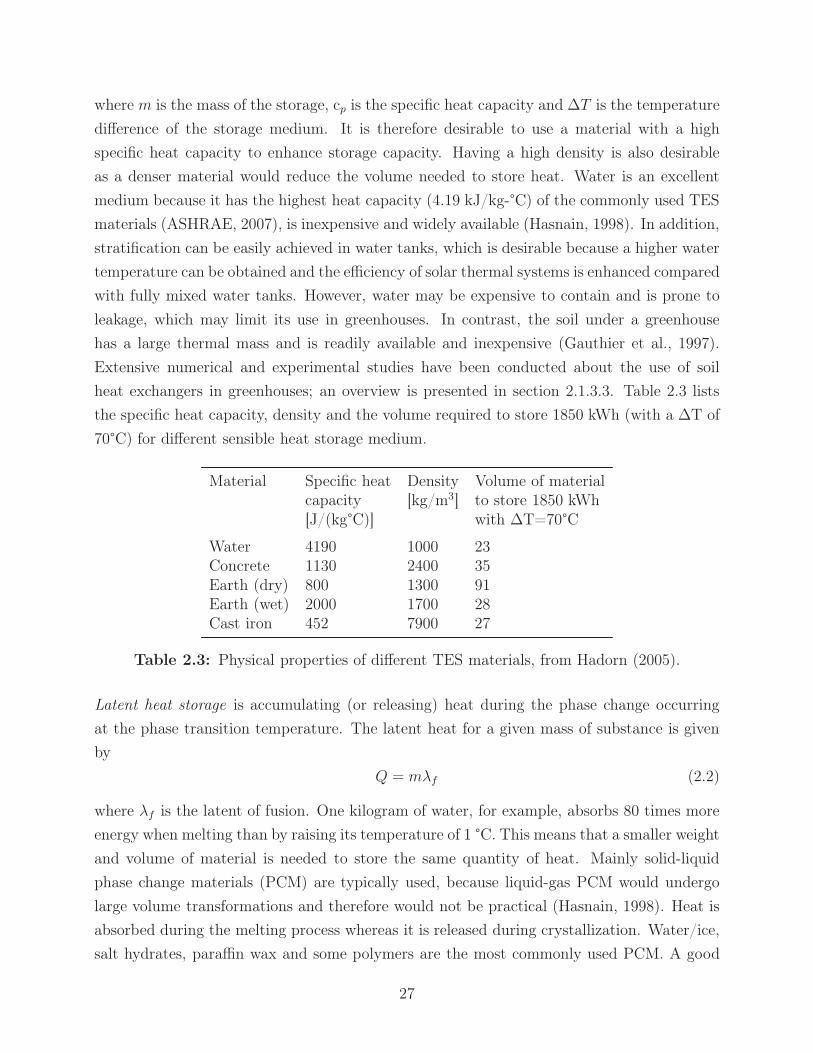
where m is the mass of the storage, cp is the specific heat capacity and ΔT is the temperature

difference of the storage medium. It is therefore desirable to use a material with a high

specific heat capacity to enhance storage capacity. Having a high density is also desirable

as a denser material would reduce the volume needed to store heat. Water is an excellent

medium because it has the highest heat capacity (4.19 kJ/kg-°C) of the commonly used TES

materials (ASHRAE, 2007), is inexpensive and widely available (Hasnain, 1998). In addition,

stratification can be easily achieved in water tanks, which is desirable because a higher water

temperature can be obtained and the efficiency of solar thermal systems is enhanced compared

with fully mixed water tanks. However, water may be expensive to contain and is prone to

leakage, which may limit its use in greenhouses. In contrast, the soil under a greenhouse

has a large thermal mass and is readily available and inexpensive (Gauthier et al., 1997).

Extensive numerical and experimental studies have been conducted about the use of soil

heat exchangers in greenhouses; an overview is presented in section 2.1.3.3. Table 2.3 lists

the specific heat capacity, density and the volume required to store 1850 kWh (with a ΔT of

70°C) for different sensible heat storage medium.

Material Specific heat Density Volume of materialcapacity [kg/m3] to store 1850 kWh[J/(kg°C)] with ΔT=70°C

Water 4190 1000 23Concrete 1130 2400 35Earth (dry) 800 1300 91Earth (wet) 2000 1700 28Cast iron 452 7900 27

Table 2.3: Physical properties of different TES materials, from Hadorn (2005).

Latent heat storage is accumulating (or releasing) heat during the phase change occurring

at the phase transition temperature. The latent heat for a given mass of substance is given

by

Q = mλf (2.2)

where λf is the latent of fusion. One kilogram of water, for example, absorbs 80 times more

energy when melting than by raising its temperature of 1 °C. This means that a smaller weight

and volume of material is needed to store the same quantity of heat. Mainly solid-liquid

phase change materials (PCM) are typically used, because liquid-gas PCM would undergo

large volume transformations and therefore would not be practical (Hasnain, 1998). Heat is

absorbed during the melting process whereas it is released during crystallization. Water/ice,

salt hydrates, paraffin wax and some polymers are the most commonly used PCM. A good

27

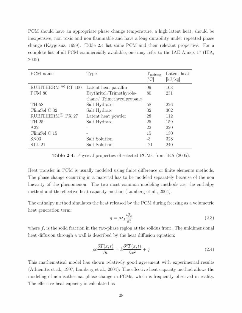
PCM should have an appropriate phase change temperature, a high latent heat, should be

inexpensive, non toxic and non flammable and have a long durability under repeated phase

change (Kaygusuz, 1999). Table 2.4 list some PCM and their relevant properties. For a

complete list of all PCM commercially available, one may refer to the IAE Annex 17 (IEA,

2005).

PCM name Type Tmelting Latent heat[°C] [kJ/kg]

RUBITHERM ® RT 100 Latent heat paraffin 99 168PCM 80 Erythritol/Trimethyrole- 80 231

thane/ TrimethyrolpropaneTH 58 Salt Hydrate 58 226ClimSel C 32 Salt Hydrate 32 302RUBITHERM® PX 27 Latent heat powder 28 112TH 25 Salt Hydrate 25 159A22 - 22 220ClimSel C 15 - 15 130SN03 Salt Solution -3 328STL-21 Salt Solution -21 240

Table 2.4: Physical properties of selected PCMs, from IEA (2005).

Heat transfer in PCM is usually modeled using finite difference or finite elements methods.

The phase change occurring in a material has to be modeled separately because of the non

linearity of the phenomenon. The two most common modeling methods are the enthalpy

method and the effective heat capacity method (Lamberg et al., 2004).

The enthalpy method simulates the heat released by the PCM during freezing as a volumetric

heat generation term:

q = ρλfdfs

dt(2.3)

where fs is the solid fraction in the two-phase region at the solidus front. The unidimensional

heat diffusion through a wall is described by the heat diffusion equation:

ρc∂T (x, t)

∂t= k

∂2T (x, t)

∂x2+ q (2.4)

This mathematical model has shown relatively good agreement with experimental results

(Athienitis et al., 1997; Lamberg et al., 2004). The effective heat capacity method allows the

modeling of non-isothermal phase change in PCMs, which is frequently observed in reality.

The effective heat capacity is calculated as

28

ceff =λf

T2 − T1+ cp (2.5)

where T1 is the temperature where melting (or solidification) begins and T2 is the temperature

at which the material is totally melted (or solidified). The effective heat capacity can be

calculated separately for melting and freezing processes. The energy balance equation with

initial and boundary conditions can be found in Lamberg et al. (2004). After comparing

numerical models with experiments, they concluded that the effective heat capacity method

with a narrow temperature range (ΔT = 2°C) is the most precise method.

Hed and Bellander (2006) presented a mathematical model of a PCM air heat exchanger.

They defined a fictive convective heat transfer coefficient as

h∗c =vair A ρ cp(1 − e

P ULvair A ρ cp )

P L(2.6)

where A, P and L are the area, perimeter and length of the heat exchanger and U is the heat

transfer coefficient between the middle of PCM and the air. The advantage of this method

lies in the fact that this fictive heat transfer coefficient can be easily integrated within existing

building energy simulation software.

2.1.3.2 Thermal storage sizing strategies

One existing method for sizing TES systems is based on the thermal admittance of a mul-

tilayered wall (Athienitis, 1994). The the self and transfer admittance of a wall are transfer

functions particularly useful to analyze the effects of cyclic varying conditions (like solar

radiation and temperature) under steady periodic conditions. In solaria and greenhouses,

internal heat storage elements are absorbing and releasing heat from the same surface. In

this case, we are mainly interested in the self-admittance, which relates the effect of a heat

source at one surface to the temperature of the same surface. The self-admittance Ys is given

by the ratio of the heat flow at the interior surface divided by the temperature of that same

surface

Ys =Qinside

Tinside(2.7)

For a wall section made of an insulating and a thermally massive layer, as depicted in figure

2.6, the self-admittance is calculated with

Ys =A

[U + kγntanh(γnL)

]U

kγntanh(γnL) + 1

(2.8)

29

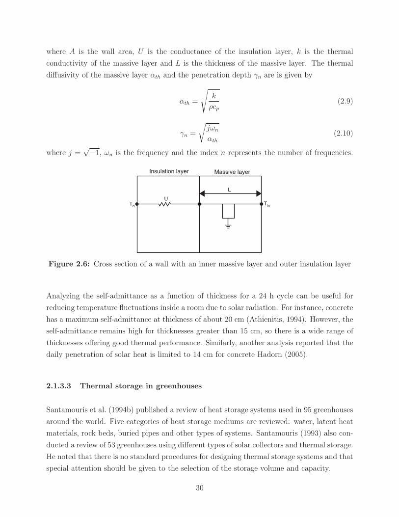
where A is the wall area, U is the conductance of the insulation layer, k is the thermal

conductivity of the massive layer and L is the thickness of the massive layer. The thermal

diffusivity of the massive layer αth and the penetration depth γn are is given by

αth =

√k

ρcp

(2.9)

γn =

√jωn

αth(2.10)

where j =√−1, ωn is the frequency and the index n represents the number of frequencies.

Figure 2.6: Cross section of a wall with an inner massive layer and outer insulation layer

Analyzing the self-admittance as a function of thickness for a 24 h cycle can be useful for

reducing temperature fluctuations inside a room due to solar radiation. For instance, concrete

has a maximum self-admittance at thickness of about 20 cm (Athienitis, 1994). However, the

self-admittance remains high for thicknesses greater than 15 cm, so there is a wide range of

thicknesses offering good thermal performance. Similarly, another analysis reported that the

daily penetration of solar heat is limited to 14 cm for concrete Hadorn (2005).

2.1.3.3 Thermal storage in greenhouses

Santamouris et al. (1994b) published a review of heat storage systems used in 95 greenhouses

around the world. Five categories of heat storage mediums are reviewed: water, latent heat

materials, rock beds, buried pipes and other types of systems. Santamouris (1993) also con-

ducted a review of 53 greenhouses using different types of solar collectors and thermal storage.

He noted that there is no standard procedures for designing thermal storage systems and that

special attention should be given to the selection of the storage volume and capacity.

30

A more recent review of heating systems for greenhouses has been carried out by Sethi and

Sharma (2008). This review covers water storage systems, rock beds, PCM, earth-to-air

heat exchangers (EAHE) and north walls. Correlations of storage volume of different storage

media for a given greenhouse area and cover type have been generated from the collected

information. The authors are suggesting that these correlations can be used at an early

design stage to provide an approximate value of the required storage volume.

As mentioned is section 2.1.1, it was observed that greenhouses are more efficient when

having their longest side facing south. For a fully glazed greenhouse with a south orientation,

radiation entering from the south side can exit the greenhouse through the north side. This

effect can have a large impact especially for narrow greenhouses. Having an opaque north

wall enhances solar radiation collection in a greenhouse and can reduce heat losses if well

insulated. Some studies suggested to make this wall reflective (Thomas, 1978; Lawand et al.,

1975), while others promoted the idea of using this location for passive thermal storage

(Tiwari et al., 1988; Singh and Tiwari, 2000; Beshada and Zhang, 2006). It was shown that

having thermal storage on the north wall can significantly increase thermal load levelling

(Tiwari et al., 1988). A review of the use of north walls for absorption or reflection of solar

radiation revealed a 1-10°C air temperature increase and a 35-82% heating needs reduction

(Sethi and Sharma, 2008).

China has a long tradition of local cultivation using so-called chinese solar greenhouses (CSG).

These greenhouses have all adopted a similar design, which includes a plastic film covering

the slanted south roof, a thermal blanket deployed at night and a thermally massive north

wall. The exposed soil on the ground also contributes to thermal load leveling, although

uninsulated. The north walls in CSG are usually made of bricks or earth; brick walls are

generally 0.4-0.8 m thick while earth walls can be as thick as 5.5 m (Tong et al., 2013).

In a review of EAHE systems installed in greenhouses, reported energy savings of 28% to

62% and air temperature increase of 3-10°C have been reported. Pipes are usually made of

plastic but aluminum and concrete have also been tested. Typically one or two rows of pipes

are placed 0.4-2.1 m below the ground (Sethi and Sharma, 2008).

A brief overview of previous mathematical models of EAHE and their limitations is presented

by Gauthier et al. (1997). They presented a new model with the capability to predict transient

three dimensional heat transfer. The model can simulate non homogenous soil properties,

concrete foundation and insulation as well as condensation and evaporation in the pipes.

This model is then used to conduct a parametric study on the design and control of EAHE.

Their results revealed that adding perimeter and under slab insulation increased the energy

recovery ratio from 0.66 to 0.92.31

Kurata and Takakura (1991) conducted simulations to evaluate the performance of under-

ground seasonal thermal storage in greenhouses. They compared the same greenhouse op-

erated in seasonal storage mode (with water-based solar thermal collectors used to charge

the TES and air ducts for heat extraction) and in daily mode (with air ducts for charg-

ing/discharging the TES only). They found that the energy used for circulating air and

pumping water was more then the heating energy saved when the underground TES was

used in seasonal storage mode, while that the net energy savings were positive when the TES

was used in daily storage mode. It should be noted that the soil under the greenhouse used

for storing heat was not insulated and the energy required for operating pumps was very

high.

A review of greenhouses using PCM for energy storage has been conducted by Kurklu (1998).

The most commonly used PCM are CaCl2·6H2O, Na2SO2·10H2O, PEG and paraffins. The

amount of PCM used varied greatly from 4.8 kg/m2 to 83 kg/m2. Energy savings from 30%

to 80% were reported. All studies under review suggested that PCM can be efficiently used

for energy storage and humidity control in greenhouses.

A study conducted by Öztürk (2005) focused on characterizing the energy and exergy effi-

ciencies of a seasonal latent heat storage system for an experimental 180 m2 greenhouse in

Turkey. They studied paraffin (with melting temperatures of 45°- 60°) coupled to a 27 m2

solar thermal collector array. The greenhouse was filled with 6000 kg of paraffin, an equiva-

lent of 33.33 kg/m2. They obtained an average net energy efficiency of 40% and an average

net exergy efficiency of 4%. They concluded that exergy analysis should be used to design

thermal energy storage systems with high thermodynamic efficiencies.

2.1.4 Auxiliary heating systems

Even with a good passive solar design, auxiliary heating might be needed, especially if com-

mercial crops are to be grown. In Canada, the total greenhouse operating expenses in 2010

reached 2.1 billions, from which 14% was spent for electricity, natural gas, heating oil and

other fuels. Natural gas heating is the most common option in Canada and represents 61%

of all expenses for heating fuels and electricity (Statistics Canada, 2010).

Some innovative and sustainable heating systems/strategies have been designed and imple-

mented in greenhouses; the most promising options are briefly described in this section.

Introducing animals in greenhouses may be beneficial by adding sensible (and latent) heat

into the system. Heat production from animals is between 1.5-21 W/kg, the former being

32

representative of the lower limit for dairy cows and the latter of the higher limit for young

chickens (ASHRAE, 2009, chapter 10). However, indoor air quality must be monitored and

noxious gas emitted by animals and their wastes, like ammonia (NH3) and hydrogen sulfide

(H2S), must be controlled (FAO, 1994).

Additional heat can be obtained by mixing animal manure with plant waste in a tank to pro-

duce methane and heat. The methane can be used for heating or cooking in small facilities

or for generating electricity in larger facilities. Such a system provides sound waste man-

agement, improves indoor air quality (by reducing toxic gases), and produces a high quality

fertilizer which results from the fermentation process (FAO, 1994). Kostov (1995) observed a

48-79% yield increase of cucumber production by using composting waste as growing media

compared to a control mixture. It is suggested that this effect is due to a higher nutrient

content and temperature of the compost media as well from CO2 emissions resulting from

the decomposition process.

Hong et al. (1997) have composted manure with rice hulls in a greenhouse where tomatoes

were grown in soil beds. The beds were located in rows surrounded by composting material

and were therefore heated by direct heat transfer through the soil. The soil beds temperature

was maintained between 17.5-32.5 °C while outside underground temperature was between

6-11.9 °C. The resulting composted product took 42 days to reach maturity and was suitable

for use as an organic fertilizer.

Wood biomass is a renewable source that is considered carbon neutral, since the green-

house gas (GHG) released during combustion has been absorbed from the atmosphere dur-

ing growth. Therefore, no additional GHG are released into the atmosphere during their

combustion (when neglecting the energy required for transportation and transformation of

the biomass). According to Chau et al. (2009), the installation of a wood pellet boiler in a

greenhouse to supply up to 60% of the total heat demand is economical for average or large

greenhouses (7.5-15 ha) in Canada. As flue gas from natural gas boilers is often injected

inside greenhouses for CO2 enrichment (to enhance crop growth), the authors assumed that

displacing 100% of natural gas with wood pellets would require buying liquid CO2 for enrich-

ment, which may not be economically feasible. However, many methods for CO2 recovery

from the exhaust gas of biomass heating systems exist. Dion et al. (2011) published a review

of these methods for safe CO2 enrichment in greenhouses. While they concluded that future

research is needed to optimize safe and clean CO2 enrichment from biomass heating systems,

they pointed out that improving biomass boiler efficiency, using scrubbers to clean NOx and

SOx and using membrane separation techniques to prevent fine particles are viable techniques

for reducing the overall carbon footprint of greenhouse plant production.

33

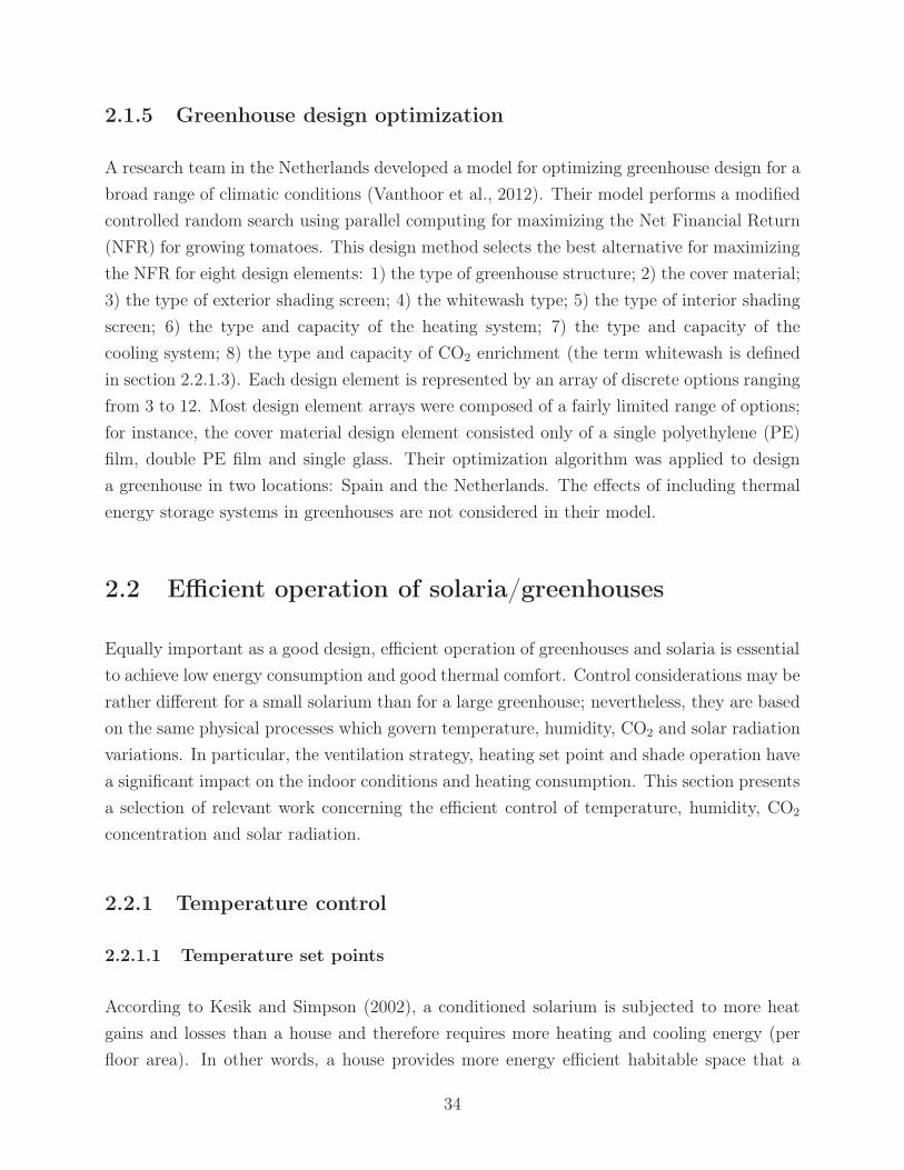
2.1.5 Greenhouse design optimization

A research team in the Netherlands developed a model for optimizing greenhouse design for a

broad range of climatic conditions (Vanthoor et al., 2012). Their model performs a modified

controlled random search using parallel computing for maximizing the Net Financial Return

(NFR) for growing tomatoes. This design method selects the best alternative for maximizing

the NFR for eight design elements: 1) the type of greenhouse structure; 2) the cover material;

3) the type of exterior shading screen; 4) the whitewash type; 5) the type of interior shading

screen; 6) the type and capacity of the heating system; 7) the type and capacity of the

cooling system; 8) the type and capacity of CO2 enrichment (the term whitewash is defined

in section 2.2.1.3). Each design element is represented by an array of discrete options ranging

from 3 to 12. Most design element arrays were composed of a fairly limited range of options;

for instance, the cover material design element consisted only of a single polyethylene (PE)

film, double PE film and single glass. Their optimization algorithm was applied to design

a greenhouse in two locations: Spain and the Netherlands. The effects of including thermal

energy storage systems in greenhouses are not considered in their model.

2.2 Efficient operation of solaria/greenhouses

Equally important as a good design, efficient operation of greenhouses and solaria is essential

to achieve low energy consumption and good thermal comfort. Control considerations may be

rather different for a small solarium than for a large greenhouse; nevertheless, they are based

on the same physical processes which govern temperature, humidity, CO2 and solar radiation

variations. In particular, the ventilation strategy, heating set point and shade operation have

a significant impact on the indoor conditions and heating consumption. This section presents

a selection of relevant work concerning the efficient control of temperature, humidity, CO2

concentration and solar radiation.

2.2.1 Temperature control

2.2.1.1 Temperature set points

According to Kesik and Simpson (2002), a conditioned solarium is subjected to more heat

gains and losses than a house and therefore requires more heating and cooling energy (per

floor area). In other words, a house provides more energy efficient habitable space that a

34

solarium, regardless of its orientation or insulation level. This is of paramount importance

when designing attached solaria; even with an energy efficient design, a solarium should not

be conditioned like a house if a low energy consumption is an important design objective. In

this case, temperature fluctuations wider than in a normally conditioned building must be

accepted.

When auxiliary heating systems are used, many operating strategies can be employed for

reducing their energy consumption. In most cases, requirements for optimum plants envi-

ronment and minimum energy use are contradictory (Garzoli, 1989). Yet it is essential for

an energy efficient climate control to allow temperature fluctuations within a certain range

and create fluent set-points transitions (Dieleman and Hemming, 2011). In the long term, it

would be possible to breed low temperature tolerant crops, but in the short term temperature

integration is a more appropriate option (Bakker et al., 2008). As another alternative, Tantau

et al. (2011) suggested to select a cropping sequence with wintertime crops that have lower

temperature requirements to reduce the heating energy consumption of greenhouses.

The concept of temperature integration is based on the ability of plants to tolerate tem-

perature deviations from an average set point. With the typical set points for heating and

ventilation that lie between a narrow bandwidth of 1-2 °C, heating and ventilation may al-

ternate many times per day, leading to high energy consumption (Körner and Challa, 2003).

When temperature integration is applied, temperatures are allowed to fluctuate within a

certain bandwidth over a predefined time period during which the average temperature must

respect a chosen set point. This strategy may lead to energy savings of 3% for a bandwidth

of 2 °C and to 13% at a bandwidth of 10 °C without impairing crop growth (Dieleman and

Hemming, 2011). The most common temperature integration strategy employed is to use a

higher set point for ventilation to increase heating due to solar gains and to compensate by

selecting a lower set point at night or on cloudy days, which may yield energy savings of up

to 16% (Bakker et al., 2008).

According to Garzoli (1989), temperature stratification is a major problem in greenhouses.

To alleviate this problem, he suggested to supply heat directly to the roots of plants which

would allow to reduce the air temperature by 4 °C or 5 °C.

2.2.1.2 Ventilation

Greenhouses are usually ventilated to prevent high temperatures and humidity levels (Seginer,

1997), as well as to avoid carbon dioxide depletion (Garzoli, 1989). This section is treating

35

ventilation-related aspects for temperature control, while ventilation for humidity and carbon

dioxide control is treated in sections 2.2.2.1 and 2.2.3.1

Evaporative cooling may be employed when the outside temperature exceeds the maximum

desired temperature inside the greenhouse. Evaporative cooling reduces the temperature of

incoming outside air by increasing its humidity content. Both natural and forced ventilation

is common in greenhouses, but if evaporative cooling is to be employed, forced ventilation

systems are necessary. Desired ventilation rates for summer conditions are about 45-60 air

changes per hour to provide adequate temperatures for proper plant growth. Reducing the

solar radiation entering in greenhouses, by applying white paint on the glazing for instance,

lowers the ventilation rate needed for temperature control. In addition, a fully cropped green-

house has reduced ventilation needs for temperature control than an uncropped greenhouse

because of the evapotranspiration of plants, which acts as evaporative cooling (Hellickson

and Walker, 1983). Design strategies to achieve good natural ventilation are summarized in

section 2.1.1.2.

A simple equation can be used to roughly estimate the ventilation rate needed to maintain

a specific air temperature inside a greenhouse (Hellickson and Walker, 1983)

τIAf (1 − E) = (Tin − To)(UAg +

Qf

vcp

)(2.11)

where τ is the transmittance of the glazing, I is the solar intensity on a horizontal surface,

Af is the floor area, E is the ratio of evaporation to solar radiation (a value of 0.5 is rec-

ommended), U is the heat transmission coefficient, Tin and To are the indoor and outdoor

temperatures, Qf is the ventilation air flow, v is the specific volume of indoor air and cp is

the specific heat of dry air.

For an indoor temperature of 20 °C and a relative humidity of 70%, the specific volume is

0.844 m3/kg dry air. As an example, a greenhouse with floor and glass areas of 1000 m2 and

1600 m2 and a volume of 3000 m3 is considered, which is subjected to a solar radiation of

600 W/m2 with no infiltration. Inserting these values into equation 2.11 yields

0.84 · 600 · 1000(1 − 0.5) = (20 − To)(6.3 · 1600 +Qf

0.8441000) (2.12)

The relationship between the outdoor temperature and the required ventilation rate to main-

tain 20 °C inside a single and double glazed greenhouse is depicted in figure 2.7 (with U values

of 6 and 2.8 W/°C-m2 and transmittance values of 0.84 and 0.71 respectively). It can be

seen that a single glazed greenhouse with no ventilation nor infiltration would require heating

36

at temperatures below -6 °C while a double glazed greenhouse would require heating only

at temperatures below -27 °C. At one ACH, a single glazed greenhouse would need heating

below -4 °C and a double glazed greenhouse below -19 °C. This analysis shows that even on

cold bright days in the middle of winter, a greenhouse may need ventilation to prevent high

temperature (Hellickson and Walker, 1983).

Air

chan

ges

per

hour

Outdoor temperature (°C)

Single glassDouble glass

-30 -20 -10 0 10 200

10

20

30

40

50

60

Figure 2.7: Ventilation rate for maintaining inside greenhouse air temperature at 20 °C

As seen in section 2.1.1.2, achieving natural ventilation rates of 45-60 ACH for temperature

control in summer is not always possible, especially at low wind speed. In addition, such high

ventilation rates are not always desirable, especially when the outdoor relative humidity is

low, because it would induce a low relative humidity inside the greenhouse which could lead

to increased evapotranspiration and water stress (Perdigones et al., 2008) (c.f. section 2.2.2).

Solar shading materials can be used to reduce solar heat gains and therefore the ventilation

rate needed for temperature control.

2.2.1.3 Shading system

The solar radiation entering a greenhouse can be reduced by using shading compounds

sprayed on the glass or by using screening or shade materials. A description of different

shading types based on their main function is presented in section 2.1.2.4. Plants need solar

radiation between 400-700 nm, the photosythetically active radiation (PAR), as well as some

near infrared (NIR) radiation, 700-1000 nm, for morphogenesis (Kittas et al., 1999). Too

much PAR is not an issue for most plants, except for shade loving plants (Kempkes, 2008).

As noted by Nijskens et al. (1985), the ideal solar screen should have a high visible trans-

mittance and a high infrared reflectance. A low far infrared transmittance would also be

37

beneficial so that it can also be used as a thermal screen at night. The measurement of the

radiation properties of twelve shading materials revealed that all of them tend to reduce the

solar radiation the most in the visible range instead of the infrared. On the other hand, the

majority of shades showed a far infrared transmittance below 15%, indicating their suitability

to be used as night thermal screen (Nijskens et al., 1985).

The application of white paint on glass, often called whitewash, may provide about 35%

shading and does not interfere with ventilation like shading nets which negatively affect the

performance of natural ventilation (Kittas et al., 1999). However, it reduces the transmitted

PAR as well as NIR and it is applied seasonally. As a result, once applied, it always reduces

the PAR, even on overcast days where it would be needed for plants growth. The applica-

tion of the whitewash must be adapted to the outdoor weather and the optimal timing for

application and removal is not easy to identify (Kempkes, 2008).

Screens can be installed inside or outside greenhouses. Outdoor screens are more efficient

for reducing solar gains and do not interfere as much with natural ventilation. However,

they need a heavy permanent structure and are more susceptible to be damaged by weather

conditions (Kempkes, 2008). Hemming et al. (2006a) pointed out that NIR filtering multilayer

coating can be applied to glass and plastic covers, but that this is not desirable in the

winter period in most climatic regions. They estimate that NIR filtering moveable screens

could be an alternative in the future, but that adequate NIR filtering materials are still not

available.

Moveable solar shades are typically controlled to be activated when the indoor temperature

and/or solar radiation exceed a certain level. Lorenzo et al. (2003, 2004) have been activat-

ing an external shade (with 49% light transmittance) when the air greenhouse temperature

reached 27-29 °C and when outside global solar radiation exceeded 650-800 W/m2. With

these set points, the global radiation incident on the crop was reduced by 20.5-36.4%, but

similar marketable yields were obtained, due to improved thermal and hygrometric conditions

provided by the screen. This may also be partly explained by the diffusion of light created

by employing shades: simulations predicted that reducing the PAR transmittance of a clear

greenhouse cover from 90% to 85% could not negatively affect yields if the 85% transmittive

cover diffuses 80% of incoming light (Hemming et al., 2006b). Simulations from Aikman

(1989) estimated even higher benefits: the redistribution of solar radiation in a crop, which

can be obtained by using screens, could give an increase of 22% in annual productivity.

Simulations conducted by Montero (2006) have shown that while evaporative cooling may be

more effective than shading for reducing indoor temperature, shading achieves greater water

38

use efficiency. It was also shown that the use of movable shading is more effective at low

ventilation rates: their contribution becomes almost negligible at ventilation rates greater

than 40 ACH, where the indoor temperature of a shaded greenhouse becomes practically

identical to an unshaded greenhouse.

A thermal screen, unlike a solar screen, should have a high solar transmittance to take

advantage of solar gains to reduce heating loads. The operating conditions of thermal screens

have a significant impact on the energy consumption. Control strategies for operating thermal

screens in greenhouses can be based on several approaches such as:

• Time clock operation;

• A fixed value of solar irradiance;

• A linear correlation between solar irradiance and outside temperature;

• An economic criteria based on energy saved versus crop lost;

• An energy balance on the glazing.

It was found that energy savings can be increased by 6% when the screen is controlled based

on radiation level compared to time clock operation (Seginer and Albright, 1980). Marsh

et al. (1984) measured an energy saving of 3.3% when the opening of thermal screens was

based on an inside light level of 30 W/m2 compared to time clock operation. They also

concluded that using a more complicated control strategy based on a light level that is a

linear function of the outside temperature is not justified because no additional savings were

observed compared to a fixed light level control.

Simulations carried out by Dieleman and Kempkes (2006) have shown that by operating a

thermal screen opening based on outside radiation level from 1 W/m2 to 25, 50 and 150 W/m2,

additional energy savings of 2%, 3% and 4% can be achieved. They also found that operating

a screen based on correlations of outside temperature and radiation can achieve a similar

energy reduction of up to 4% compared to an operation strategy based on a fixed outside

radiation level of 1 W/m2.

2.2.2 Humidity control

Plants absorb solar energy and CO2 which are converted into chemical energy by photosyn-

thesis. In addition to this process, transpiration occurs through stomata in leaves, which

serves to evaporatively cool plants. Transpiration rates depend mainly on the degree of

stomatal opening, the water vapor pressure deficit between plant leaves and air as well as air

turbulence (Hellickson and Walker, 1983).

39

The majority of plants grow best between a fairly narrow range of relative humidity levels;

typically 70% to 85% is suitable for most species. Low humidity levels increase the evaporative

demand on the plants which could lead to moisture stress, even if there is no shortage of water

in the rooting media. Very high humidities may induce condensation on the glazing and can

depress the evaporative demand on the plant and reduce nutrients uptake, which could impair

cell formation. Maintaining the RH below 85-90% could be sufficient to avoid these problems

(Garzoli, 1989).

This section covers three techniques that can be used for humidity control: conventional

ventilation, ventilation with heat recovery and the use of a solar regenerated desiccant. Other

systems such as heat pumps coupled with heat exchangers (Bakker et al., 2008) are not

covered here.

2.2.2.1 Ventilation

The traditional way of reducing the relative humidity in greenhouses is with ventilation, thus

exchanging warm and moist indoor air with cool and and dry outdoor air, which is energy

intensive (Bailey, 1984). The moisture removed by ventilation is equal to

Mwater =Qf

v(Wi − Wo) (2.13)

where Mwater is in kgwater/s and Wi and Wo is the humidity ratio of the indoor and outdoor

air. The mass of water added into the air by transpiration is given by

Mwater =EFτIAf

hfg

(2.14)

where F is the portion of the floor area covered by plants and hfg is the latent heat of

vaporization of water. The total ventilation rate Qf is equal to the ventilation rate plus the

infiltration rate:

Qf = Qf,vent + Qf,inf (2.15)

When assuming there are no condensation on the greenhouse cover, the ventilation rate for

humidity control can be calculated with

Qf =EFτIAf

ρ hfg(Wi − Wo)− Qf,inf (2.16)

40

Solar radiation (W/m2)

Air

chan

ges

per

hour

Single glassDouble glass

0 200 400 600 800 10000

2

4

6

8

10

12

Figure 2.8: Ventilation rate for maintaining inside greenhouse air at 75% RH at outdoorcondition of -20 °C and 70% RH

For the same single and double glazed greenhouses of 1000 m2 as described in section 2.2.1.2,

the ventilation rate needed to maintain 75% RH as a function of incident solar radiation is

depicted in figure 2.8 (where F=0.8). It can be seen that with To =-20 °C, the number of

air changes per hour required for humidity control is approximately 100 times less than the

incoming solar radiation. For instance, a single glazed greenhouse would require about 6 ACH

when subjected to a solar radiation level of 600 W/m2. The maximum ventilation rate for

humidity control is set to 10 ACH for most growers (de Halleux and Gauthier, 1998).

There are many ways to reduce the ventilation rate required for humidity control, such as

selecting a higher indoor humidity set point, reducing the transpiration level of plants and

dehumidifying with heat recovery. While higher humidity levels may increase the risk of

fungal diseases, it may also favor crop production and quality. It was estimated that an

increase of 5% of the RH level can reduce the energy consumption by 5 to 6% (Bakker

et al., 2008) and increasing the maximum humidity level from 80% to 85% reduces the

dehumidification needs by 30% (Campen, 2009). The transpiration rate can be decreased by

a controlled reduction of the leaf area for crops with a high leaf area index. An experiment

conducted with tomatoes revealed that when halving the leaf area by removing old leaves,

the transpiration rate was reduced by 30% without affecting crop yield.

2.2.2.2 Ventilation with heat recovery

Typical dehumidification is achieved by cooling air below its dew point temperature, thereby

condensing moisture until the desired humidity level is reached. However, air is frequently

overcooled and then must be heated to meet thermal comfort, which lead to inefficiencies

and high energy consumption.

41

Ventilation with heat recovery might be more appropriate than typical dehumidification

for solaria and greenhouses. In cold weather, the ventilated air must be heated, which

represents a significant fraction of heating costs: about 13-18% of heating costs of standard

greenhouses are due to ventilation for humidity control. Heat exchangers can be used to

recover some of the exhausted heat. Typical efficiencies of air-to-air commercial exchangers

used in Canadian agriculture are about 40%. However, they are expensive and prone to

problems at temperatures below 0 °C (Rousse et al., 2000).

Simulations conducted by de Halleux and Gauthier (1998) estimated the return on investment

for such heat exchangers to be between for 4.8-8 years and to save CDN $ 6250 per hectare

per year. Rousse et al. (2000) designed a simple air-to-air counter-flow multi-tube heat

exchanger for greenhouses located in cold climates. The experimental heat exchanger, buried

in the ground, operated at 0.5 and 0.9 ACH and reached efficiencies of 78-84%. The heat

exchanger was inexpensive, easy to assemble and maintain, could resist corrosion and mold

propagation and could operate satisfactorily even at sub zero temperatures.

A similar study conducted by Speetjens in 2001 used a heat exchanger installed in the gutter

of a greenhouse were 60-70% of sensible heat was recovered (Campen et al., 2003). A study

carried by Campen et al. (2003) about different methods for dehumidifying greenhouses in

cold climates simulated the use of an ideal heat exchanger with 100% efficiency. They found

that, depending on the crop, 108-190 MJ/m2 can be saved for a single layer greenhouse and

between 145-278 MJ/m2 for a double layer greenhouse. The energy cost reduction ranged

from 0.31-0.84 e /m2 to 0.44-1.33 e /m2. They concluded that forced ventilation with heat

exchange is the most promising dehumidification method for cold climates, but that a low

cost and efficient system need to be developed.

2.2.2.3 Solar regenerated desiccant

Dehumidification can also been achieved using solid or liquid desiccants. In this case, moisture

contained in the air is absorbed/adsorbed by the desiccant, which then must be regenerated

with a source of heat to evacuate moisture.

Solid desiccants can typically provide a higher degree of dehumidification; they are usually

made of stationary beds or rotary wheel beds. Solar air heaters are well suited for provid-

ing heat to these systems because air is the regeneration medium (Ahmed, 2005). Liquid

desiccants require lower regeneration temperatures which facilitates their coupling with low

temperature sources like flat plate solar collectors. In addition, liquid desiccant systems have

the potential to use the desiccant solution for energy storage (Mesquita et al., 2006).42

Mathematical and numerical models of solid desiccant systems are presented by Bourdoukan

et al. (2006) and Ahmed (2005), while models for liquid desiccant systems are presented by

Mesquita et al. (2006), Yutong and Hongxing (2008) and Andrusiak and Harrison (2009).

Lychnos and Davies (2008) studied the potential of a solar powered liquid desiccant system for

greenhouses. Preliminary simulation results with a solution of magnesium chloride indicated

that a reduction of the average wet-bulb temperature of 2.2-3°C is possible.

The optimum regeneration temperature of a solar desiccant system is a tradeoff between

high solar collector efficiencies, which occur at low temperatures, and high desorption rates,

which occur at higher temperatures (Andrusiak and Harrison, 2009). The solar regenerated

liquid desiccant system studied by Yutong & Hongxing showed a higher performance under

higher latent loads, which is of particular interest for greenhouses where latent loads are

high. Lychnos & Davies estimated that solar powered liquid desiccant systems are of potential

interest for cooling and dehumidifying greenhouses, but that future work is needed to optimize

heat and mass transfers.

2.2.3 Control of CO2 concentration

The atmospheric concentration of carbon dioxide reached 390 ppm in 2010 (Lacis et al.,

2010). Many crops, such as vegetables and flowers, have shown increased growth when

subjected to elevated carbon dioxide levels of 700-1000 ppm. In a closed environment with

plants like a greenhouse, the CO2 level may be quickly depleted and reach concentration

below 200 ppm. «At such levels plant growth virtually ceases, irrespective of how ideal

is the control of all other climatic parameters. In order to maintain the concentration at

or near atmospheric concentration it is necessary to ventilate the greenhouse with outside

air [...] »Garzoli (1989). It is also possible to inject carbon dioxide in greenhouses at or

above atmospheric concentration. CO2 enrichment is a common practice which enhances

photosynthesis and thus increases yield and income (Dion et al., 2011).

2.2.3.1 Ventilation

The CO2 balance of the greenhouse air is given by (Ioslovich, 1995)

ρhdCi

dt= Cg − Cv − G (2.17)

43

where ρ is the air density, h is the effective greenhouse height, Ci is the indoor CO2 concen-

tration, Cg is the CO2 enrichment flux, Cv is the CO2 exchanged by ventilation and G is the

net photosynthesis flux (in kgCO2/m2-s). The CO2 exchanged by ventilation is proportional

to the ventilation rate Qf :

Cv = ρQf (Ci − Co) (2.18)

G from equation 2.17 characterizes the CO2 assimilation by the crop and depends on its

photosynthetic activity and respiration rate. It can be calculated with

G =εIPAR gsCi

εIPAR + gsCi

(1 − δP (Tx − Tin)2

)Φ − McropRr eνr(Ti−Tr) (2.19)

where ε is the photosynthesis efficiency (in kgCO2/JPAR), IPAR is the photosynthetically ac-

tive radiation, gs is the leaf conductance to CO2, δP is an empirical coefficient representing

the photosynthesis temperature response and Tx is the temperature at which the gross pho-

tosynthesis is maximal. In addition, Mcrop is the areic dry weight of the crop, Rr is the

respiration rate, νr is a respiration exponent and Tr is the environmental temperature. Φ is

given by

Φ = 1 − e−K LAR Mcrop (2.20)

where K is a light extinction coefficient in the canopy and LAR is the leaf area ratio. IPAR

is simply calculated from the horizontal outdoor solar radiation Iho, the average glazing

transmittance τ and the ratio of PAR to solar radiation ζ :

IPAR = τIhoζ (2.21)

For the same single and double glazed greenhouses of 1000 m2 described in section 2.2.1.2, the

ventilation rate needed to maintain 350 ppm inside the greenhouse as a function of incident

solar radiation is depicted in figure 2.9. It can be seen that the photosynthetic activity

(and therefore CO2 assimilation and ventilation needs) increases almost linearly at low solar

radiation level but a saturation effect occurs and it becomes difficult to increase plants growth

by increasing radiation at higher intensities.

The values of the parameters used in equation 2.19 are presented in table 2.5. The ratio of

IPAR over I, ζ , was observed to vary between 0.43 to 0.48, depending on the sky conditions

and time of the year (Aguiar et al., 2009); an average value of 0.46 was selected.

44

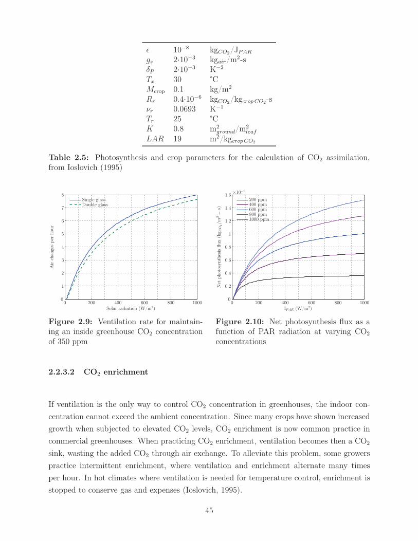
ε 10−8 kgCO2/JPAR

gs 2·10−3 kgair/m2-sδP 2·10−3 K−2

Tx 30 °CMcrop 0.1 kg/m2

Rr 0.4·10−6 kgCO2/kgcrop CO2

-sνr 0.0693 K−1

Tr 25 °CK 0.8 m2

ground/m2leaf

LAR 19 m2/kgcrop CO2

Table 2.5: Photosynthesis and crop parameters for the calculation of CO2 assimilation,from Ioslovich (1995)

Solar radiation (W/m2)

Air

chan

ges

per

hour

Single glassDouble glass

0 200 400 600 800 10000

1

2

3

4

5

6

7

8

Figure 2.9: Ventilation rate for maintain-ing an inside greenhouse CO2 concentrationof 350 ppm

IPAR (W/m2)

Net

phot

osyn

thes

isflu

x(k

g CO

2/m

2−

s)

200 ppm400 ppm600 ppm800 ppm1000 ppm

0 200 400 600 800 10000

0.2

0.4

0.6

0.8

1

1.2

1.4

1.6 ×10−6

Figure 2.10: Net photosynthesis flux as afunction of PAR radiation at varying CO2

concentrations

2.2.3.2 CO2 enrichment

If ventilation is the only way to control CO2 concentration in greenhouses, the indoor con-

centration cannot exceed the ambient concentration. Since many crops have shown increased

growth when subjected to elevated CO2 levels, CO2 enrichment is now common practice in

commercial greenhouses. When practicing CO2 enrichment, ventilation becomes then a CO2

sink, wasting the added CO2 through air exchange. To alleviate this problem, some growers

practice intermittent enrichment, where ventilation and enrichment alternate many times

per hour. In hot climates where ventilation is needed for temperature control, enrichment is

stopped to conserve gas and expenses (Ioslovich, 1995).

45

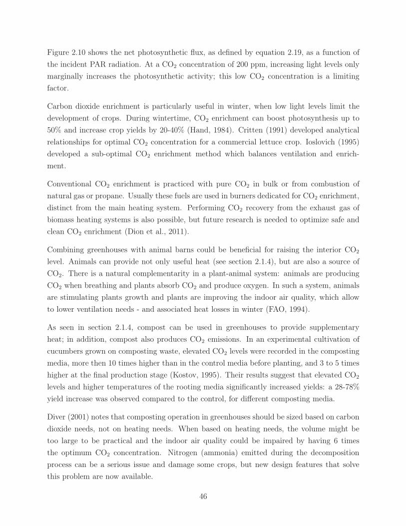
Figure 2.10 shows the net photosynthetic flux, as defined by equation 2.19, as a function of

the incident PAR radiation. At a CO2 concentration of 200 ppm, increasing light levels only

marginally increases the photosynthetic activity; this low CO2 concentration is a limiting

factor.

Carbon dioxide enrichment is particularly useful in winter, when low light levels limit the

development of crops. During wintertime, CO2 enrichment can boost photosynthesis up to

50% and increase crop yields by 20-40% (Hand, 1984). Critten (1991) developed analytical

relationships for optimal CO2 concentration for a commercial lettuce crop. Ioslovich (1995)

developed a sub-optimal CO2 enrichment method which balances ventilation and enrich-

ment.

Conventional CO2 enrichment is practiced with pure CO2 in bulk or from combustion of

natural gas or propane. Usually these fuels are used in burners dedicated for CO2 enrichment,

distinct from the main heating system. Performing CO2 recovery from the exhaust gas of

biomass heating systems is also possible, but future research is needed to optimize safe and

clean CO2 enrichment (Dion et al., 2011).

Combining greenhouses with animal barns could be beneficial for raising the interior CO2

level. Animals can provide not only useful heat (see section 2.1.4), but are also a source of

CO2. There is a natural complementarity in a plant-animal system: animals are producing

CO2 when breathing and plants absorb CO2 and produce oxygen. In such a system, animals

are stimulating plants growth and plants are improving the indoor air quality, which allow

to lower ventilation needs - and associated heat losses in winter (FAO, 1994).

As seen in section 2.1.4, compost can be used in greenhouses to provide supplementary

heat; in addition, compost also produces CO2 emissions. In an experimental cultivation of

cucumbers grown on composting waste, elevated CO2 levels were recorded in the composting

media, more then 10 times higher than in the control media before planting, and 3 to 5 times

higher at the final production stage (Kostov, 1995). Their results suggest that elevated CO2

levels and higher temperatures of the rooting media significantly increased yields: a 28-78%

yield increase was observed compared to the control, for different composting media.

Diver (2001) notes that composting operation in greenhouses should be sized based on carbon

dioxide needs, not on heating needs. When based on heating needs, the volume might be

too large to be practical and the indoor air quality could be impaired by having 6 times

the optimum CO2 concentration. Nitrogen (ammonia) emitted during the decomposition

process can be a serious issue and damage some crops, but new design features that solve

this problem are now available.

46

2.2.4 Lighting control

At high latitudes, the lack of light becomes a limiting factor in the darkest months. Growers

have to choose between interrupting their operation during such conditions or using supple-

mental lighting. The following sections describe the light requirements for adequate plants

growth, present the artificial light types most appropriate for horticulture and some control

strategies for selecting lighting levels.

2.2.4.1 Light requirements of plants

The amount of photosynthetically active radiation (PAR) is usually defined as being be-

tween 400 and 700 nm and is measured with quantum sensors that express the PAR level in

μmol/m2-s, where mol here refers to one mole of photons. For natural light, 1 μmol/m2-s

is equal to 56 lux or 0.217 W/m2 of PAR. Visible light is comprised in a larger waveband

between 380 and 770 nm.

Plants need light in three distinct spectral ranges for adequate development triggered by

photosynthesis, phototropism and photomorphogenesis. The most important photosynthetic

pigments are chlorophylls a and b with peaks at 662 and 642 nm respectively. Phototropism,

which regulates the control of plant organs and influence the orientation of plants in response

to light, is triggered by light between 400 and 500 nm. Morphogenesis, which is responsible for

healthy plant development and processes like shooting and pigment synthesis, needs far red

radiation at about 730-735 nm (Tamulaitis et al., 2005). Another study estimated that plants

also need radiation in the 700-1000 nm range for morphogenesis (Kittas et al., 1999).

In general, plants development depends on both the quantity and spectral quality of light

that is available. The daily light integral is defined as the number of photons intercepted

per square meter per day and represents the cumulative light level impinging on a crop over

a day. The use of artificial light of 100 μmol/m2-s 16 hours per day adds 5.8 mol/m2-d to

natural light. Since the daily light integral may vary between 1 and 35 mol/m2-d throughout

the year (Dorais, 2003), supplemental lighting may be necessary to maintain a more uniform

plant development all year round.

2.2.4.2 Artificial light

The most commonly used artificial light source in greenhouses is high-pressure sodium (HPS)

lamps. HPS lamps emit a wide peak at green-yellow wavelengths, but emit very little blue

47

and violet light. They have a high efficiency for converting electricity to PAR of about 26-

30%. Metal halide lamps have a wider spectrum, but a 25% lower efficiency for converting

watts to PAR and a reduced lifetime (Dorais, 2003).

Light emitting diodes (LED) have many advantages over conventional HPS lamps, such as

increased energy efficiency and durability. The high cost of LED restricted their use to specific

applications like space-based plant growth facilities, but rapidly decreasing prices indicate

that using LED in greenhouses may be feasible in the coming decades. Plants grown under

advanced high power AlGaInP LED exhibited better photosynthesis activity and morphology

then plants grown with conventional HPS lamps (Tamulaitis et al., 2005).

2.2.4.3 Radiation control

It is possible to maintain plant production if a decreasing light level is compensated by an

elevation of the carbon dioxide concentration. Such a practice could lead to significant savings

since carbon dioxide enrichment is cheaper than supplemental lighting (Both, 2000), which

would be also beneficial from en environmental point of view since it would favor carbon

sequestration over electricity consumption.

As mentioned in section 2.2.1.3, high levels of PAR are not an issue for most plants, except

for shade loving plants (Kempkes, 2008). A solar shade can be used for such crops if it is

desired to reduce the PAR level in the greenhouse.

Although artificial lighting obviously increases the electrical consumption of greenhouses, it

also reduces their heating needs. It was estimated that supplemental lighting can provide

25-41% of the heating requirements of a double plastic greenhouse in Quebec city (Dorais,

2003). Since canadian greenhouses are most frequently heated with natural gas (Statistics

Canada, 2010), displacing natural gas by electricity may reduce carbon dioxide emissions

(Dorais, 2003), especially when hydroelectricity is used.

The lighting intensity should be adapted for each crops. Light integrals of 12 mol/m2-d or

higher are generally needed for lettuce production and obtained with supplemental lighting

of 50-100 μmol/m2-s. For cucumber, it was estimated that the maximum income would occur

when using 120-150 μmol/m2-s of supplemental light. Tomato has higher light requirements:

30 mol/m2-d or higher is often reported for tomato culture (Dorais, 2003). When subjected

to the same daily light integral, radish and Chrysanthemum have shown higher dry matter

accumulation under a 18 hours lighting regime than under 12 and 24 hours. However, corn

and cucumber exhibited the same dry matter accumulation under a photoperiod of 12, 18

48

and 24 hours while, for all four species, the dry matter development was lowest with a 8

hours photoperiod (Warrington and Norton, 1991).

The installed lighting capacity is usually between 100-200 W/m2. Lamps are usually turned

off when the solar radiation level reach 240-300 W/m2 and when the daily light integral

reach 55 mol/m2-d. Photoperiods of 12-18 hours are frequently adopted, depending on the

crops (Dorais, 2003). It is generally better to have lower lighting levels during an extended

period of time up to 18-20 hours, while continuous lighting should be avoided because of

the apparition of growth abnormalities observed with some species (Warrington and Norton,

1991).

The use of artificial lighting in greenhouses may be an issue especially in urban areas because

of the light pollution they may produce (Pearson et al., 2010). In the Netherlands, legislation

requires the installation of opaque screens to reduce light transmission through greenhouse

cover by 95% and the limitation of the lighting regime to 180 μmol/m2-s, unless light pollution

is totally prevented (Van Ooster et al., 2008). Light pollution is linked to diverse ecological

impacts such as influences on organismal movements, foraging, interspecific interactions,

communication, reproduction and mortality (Gaston et al., 2012).

The use of artificial lighting in greenhouses may increase yields significantly, but is energy

and capital intensive. Therefore, high yield must be maintained to justify its use. All

greenhouse parameters must be carefully controlled, including CO2 levels, temperature and

humidity, daily temperature evolution, crop schedule and pest management (Dorais, 2003).

As depicted in figure 2.10, practicing CO2 enrichment allows to make a better use of increased

PAR radiation.

2.2.5 Greenhouse climate control models

The main variables affecting plants growth inside a greenhouse are the air temperature, hu-

midity, CO2 concentration and solar radiation level. These parameters can be controlled

via various systems such as heating systems, ventilation (natural or forced) systems, dehu-

midification or evaporative cooling systems, artificial lights, CO2 injection equipment and

thermal/solar screens. The state of these variables will determine crop yields, energy con-

sumption and net profits.

The modification of one system element often impact more than one variable. Sometimes,

modifying a system will improve some variables while impairing others. For instance, arti-

ficial lighting in winter increases radiation level and interior temperature, effects which are

49

both beneficial for increasing yields. However, artificial lighting in summer is beneficial for

increasing yield, but the associated temperature rise is detrimental.

One climate control strategy is to control the processes rather than the state of the variables.

Partial optimization can also be used to improve indoor climate when considering parameters

individually (Trigui, 2000).

Many different climate control strategies, models and programs have been developed and

published. A list of some greenhouse models developed in 1988 and before is presented in

de Halleux (1989). The simpler models consider only the energy balance of the indoor air,

but more complex models also carry out the energy balance of other elements like the glazing

cover, soil and plants. Multi elements models can be either static or dynamic. Only dynamic

models can adequately represent indoor conditions on a short time scale and are therefore

preferred (de Halleux, 1989).

Models for determining optimal temperature set points (Seginer et al., 1991), crop transpira-

tion rate (Jolliet and Bailey, 1992; Stanghellini and Van Meurs, 1992), humidity levels (Jolliet,

1994; Korner, 2003), CO2 concentration (Critten, 1991; Ioslovich, 1995) and ventilation rates

(Seginer, 1997) have been developed. Models for predicting climate inside greenhouses have

been developed by Zhang (1997), Wang and Boulard (2000) and Salazar and Rojano (2008),

while others have used existing building energy simulation software for predicting indoor

climate like TRNSYS (Carlini and Castellucci, 2010). Crop transpiration models have been

developed by Jolliet (1993) and Sánchez et al. (2009).

The indoor climate should be controlled such as to maximize crop production and minimize

energy use. However, these two objectives are often conflictive, therefore climate control

becomes an optimization problem. Ioslovich and Seginer (1998) developed a sub-optimal

method for climate control which was solved with an optimization routine. Trigui (2000)

developed a control strategy based on the maximization of an objective function to maximize

the net profit, estimated as the harvest value minus the cost of maintaining the climatic

conditions.

Aaslyng et al. (2003) developed a climate control system based on a combination of control

methods. Thermal screens were controlled to maximize profit which was calculated as a

tradeoff of the energy saved with screens on versus the production loss caused by decreased

irradiance. The allowable temperature fluctuations were considerably higher than usual; the

temperature set point was lower on cloudy days were growth is reduced and higher on sunny

days to increase production. Temperature and CO2 set points are selected in order to achieve

a desired photosynthetic level for a given irradiance and minimize heat and CO2 inputs. The

50

model is divided into components which contain mathematical models for the control of

biological phenomena or processes. Field trials showed significant energy savings with only

small changes in plant production.

2.2.6 Closed, semi-closed and open Greenhouses

As explained in the previous sections, most greenhouses rely on ventilation through the

opening of windows to control humidity, temperature and CO2 levels. However, such practices

result inevitably in sub-optimal conditions for either temperature or humidity (de Zwart,

2008). When CO2 enrichment is practiced, its efficiency is seriously altered by the opening

of windows. In addition, during the cold season, opening windows for temperature control

results in wasted solar heat which would be needed later on at night.

These observations led to the development of a new concept in the Dutch greenhouse indus-

try: the so-called closed greenhouse. Such greenhouses are equipped with a heat pump, air

treatment units with heat exchangers, air distribution ducts, daytime thermal storage and

an underground aquifer for seasonal storage. The temperature is controlled by active cooling

instead of ventilation. Energy savings of up to 30% and production increases by up to 20%

have been reported. The production increase is mainly explained by the elevated CO2 levels

that can be achieved in closed greenhouses. The economic feasibility of this concept depends

highly on the production increase that can be obtained, since typically a 10% increase in yield

represents much more money than a 10% energy savings (Heuvelink and Bakker, 2008).

In closed greenhouses, the air is cooled and dehumidified by air treatment units. A semi-

closed greenhouse has a smaller cooling capacity than a closed greenhouse, where in this

case ventilation through windows is used when the temperature is too high to be controlled

by the cooling system only. Yield increase occurs mainly during the summer, where the

combination of high solar radiation and high CO2 is possible only in closed greenhouses

(Qian et al., 2011). Experimental yields of a closed greenhouse compared to simulated yields

of conventional open greenhouses estimated a primary energy use reduction of 19% for a

stand-alone closed greenhouse and of 33% when coupled to open greenhouses covering twice

the area (Opdam et al., 2005).

Besides energy savings and increased production, closed greenhouses have a high water effi-

ciency (no water loss), offer a better temperature control and could reduce or eliminate the

need for pesticides (Gelder et al., 2005). However, in 1995, an entirely closed greenhouse

51

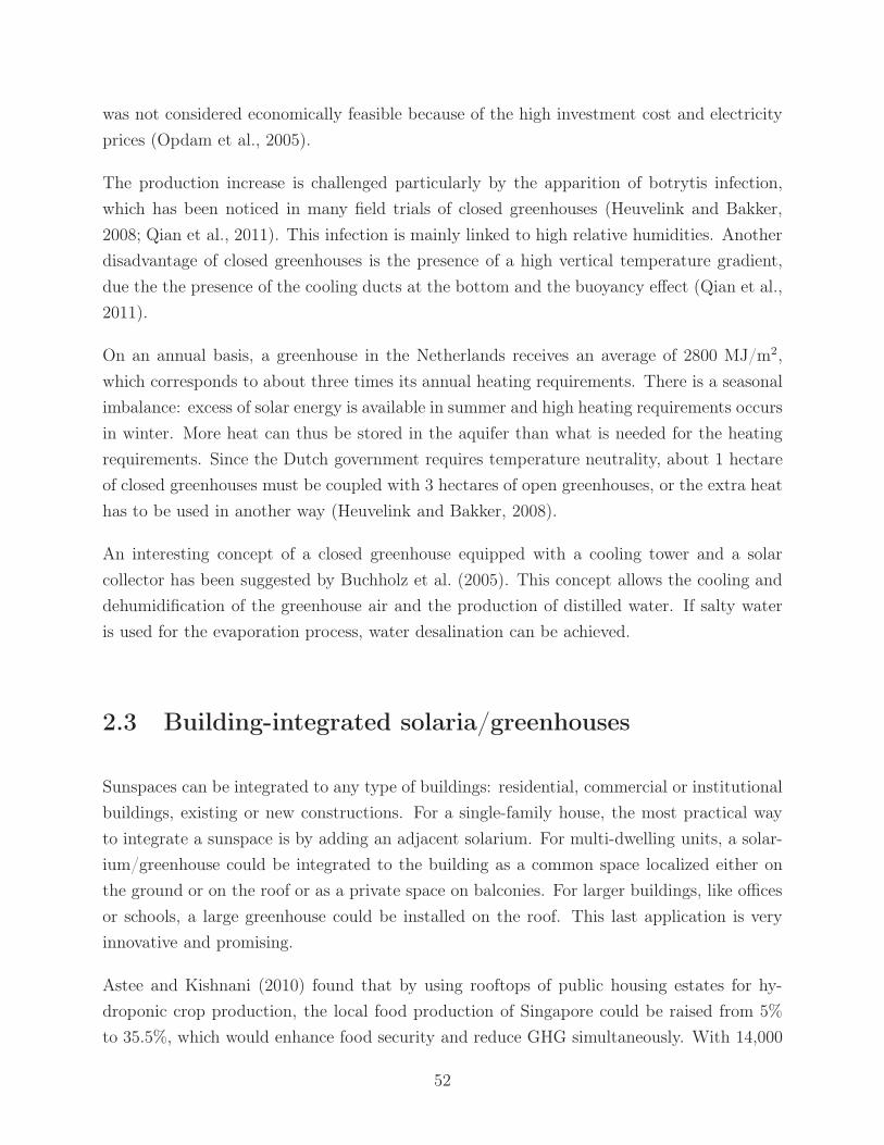
was not considered economically feasible because of the high investment cost and electricity

prices (Opdam et al., 2005).

The production increase is challenged particularly by the apparition of botrytis infection,

which has been noticed in many field trials of closed greenhouses (Heuvelink and Bakker,

2008; Qian et al., 2011). This infection is mainly linked to high relative humidities. Another

disadvantage of closed greenhouses is the presence of a high vertical temperature gradient,

due the the presence of the cooling ducts at the bottom and the buoyancy effect (Qian et al.,

2011).

On an annual basis, a greenhouse in the Netherlands receives an average of 2800 MJ/m2,

which corresponds to about three times its annual heating requirements. There is a seasonal

imbalance: excess of solar energy is available in summer and high heating requirements occurs

in winter. More heat can thus be stored in the aquifer than what is needed for the heating

requirements. Since the Dutch government requires temperature neutrality, about 1 hectare

of closed greenhouses must be coupled with 3 hectares of open greenhouses, or the extra heat

has to be used in another way (Heuvelink and Bakker, 2008).

An interesting concept of a closed greenhouse equipped with a cooling tower and a solar

collector has been suggested by Buchholz et al. (2005). This concept allows the cooling and

dehumidification of the greenhouse air and the production of distilled water. If salty water

is used for the evaporation process, water desalination can be achieved.

2.3 Building-integrated solaria/greenhouses

Sunspaces can be integrated to any type of buildings: residential, commercial or institutional

buildings, existing or new constructions. For a single-family house, the most practical way

to integrate a sunspace is by adding an adjacent solarium. For multi-dwelling units, a solar-

ium/greenhouse could be integrated to the building as a common space localized either on

the ground or on the roof or as a private space on balconies. For larger buildings, like offices

or schools, a large greenhouse could be installed on the roof. This last application is very

innovative and promising.

Astee and Kishnani (2010) found that by using rooftops of public housing estates for hy-

droponic crop production, the local food production of Singapore could be raised from 5%

to 35.5%, which would enhance food security and reduce GHG simultaneously. With 14,000

52

acres of unshaded large rooftops, New York City could produce enough vegetables to feed

over 30 million people, more than 3 times its population (Droege et al., 2009).

Caplow is the first researcher to use the term building-integrated greenhouse in a conference

paper published in 2007 (Caplow and Nelkin, 2007). Only a few experimental and commercial

rooftop greenhouses have been built so far. Montreal is hosting the first commercial rooftop

greenhouse, which began its operation in 2011 (Rifkin, 2011). A few months later, another

company built and started to operate a rooftop greenhouse in Brooklyn, New York (Foderado,

2012). Some other young companies have been created recently and are planning to buid

a first rooftop greenhouse in the near future. Others companies developed another concept

allowing to grow food in buildings, but without a greenhouse. It is possible to grow leafy

vegetables in a box, vertically to enhance density, where artificial light and all other climatic

parameters are carefully controlled (The Produce News, 2011).

Although the first commercial rooftop greenhouses of Montreal and Brooklyn are siting on

top of a building, they are not truly integrated. The greenhouse structure literally sits over

the roof, on which rubber mats have simply been added in Montreal. The heating system of

the greenhouses is totally disconnected from the heating and cooling systems of the building

beneath. These greenhouses are typical of good quality new greenhouses that are built in

North America, but are not as efficient as the best commercial greenhouses in northern Europe

like the Netherlands. They are equipped of some energy saving features, like thermal screens,

but they have no special features compared to stand alone greenhouses. At the Montreal site,

the growers estimate a reduction of 50% of their heating needs thanks to the heat losses of the

building beneath (Hage, 2011). When greenhouses are overheating, windows simply open,

which happen even in winter. The potential of using extra heat from the greenhouse to

supply auxiliary heating to the building beneath has not been investigated.

Structural considerations have to be taken into account when adding greenhouses above

existing buildings. Some buildings would require structural reinforcement to carry the added

load, which would add significant cost to a project, but some existing buildings have the

capacity to support such an additional load. Snow loads are not an issue with single glazed

greenhouses because the snow melts very quickly upon contact with the warm glass. However,

energy efficient greenhouses with double glazing and/or thermal curtains are slowing down

snow melting. Some greenhouses equipped with thermal curtains usually supply heat only

to the space below the curtains, to reduce heat loads, but have dedicated heat pipes above

the curtains used only for melting snow. Structural loads due to snow must be considered in

cold climates and especially for energy efficient rooftop greenhouses.

53

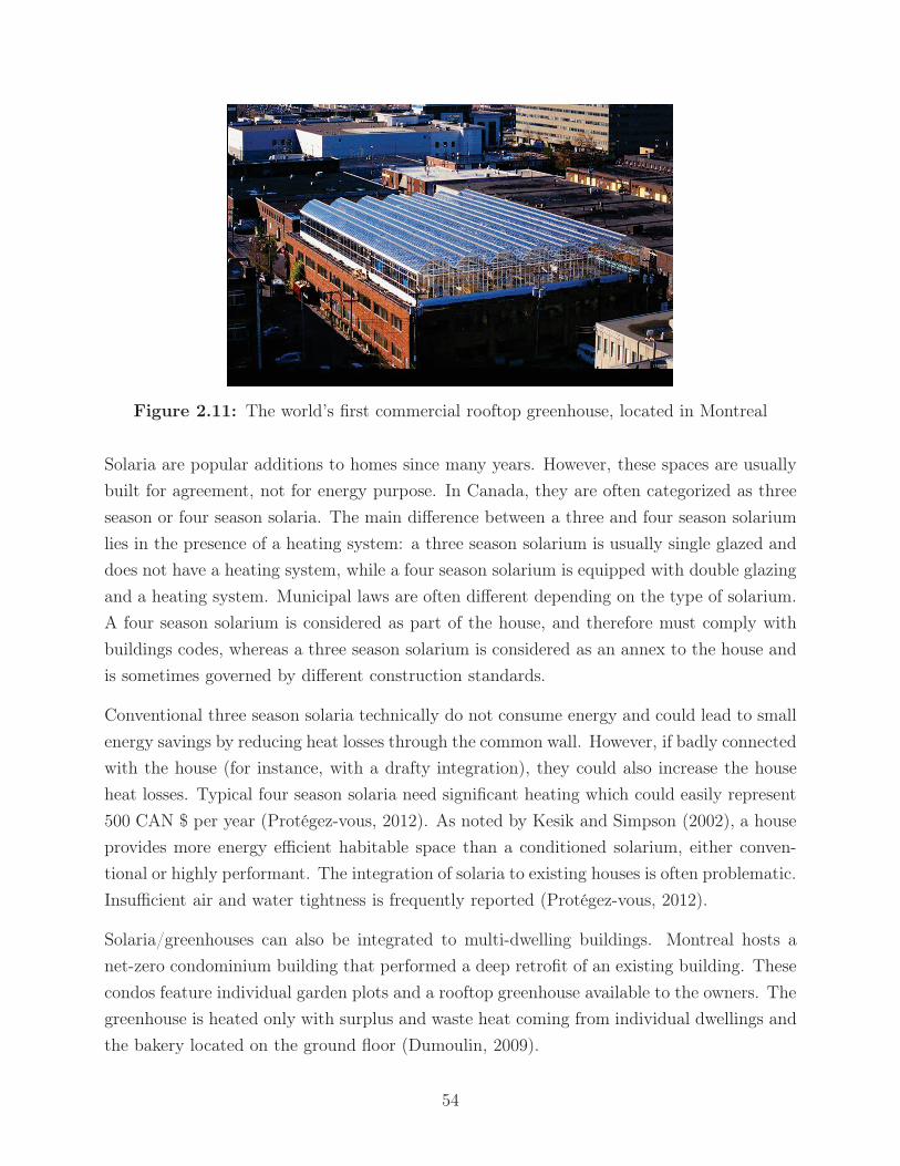
Figure 2.11: The world’s first commercial rooftop greenhouse, located in Montreal

Solaria are popular additions to homes since many years. However, these spaces are usually

built for agreement, not for energy purpose. In Canada, they are often categorized as three

season or four season solaria. The main difference between a three and four season solarium

lies in the presence of a heating system: a three season solarium is usually single glazed and

does not have a heating system, while a four season solarium is equipped with double glazing

and a heating system. Municipal laws are often different depending on the type of solarium.

A four season solarium is considered as part of the house, and therefore must comply with

buildings codes, whereas a three season solarium is considered as an annex to the house and

is sometimes governed by different construction standards.

Conventional three season solaria technically do not consume energy and could lead to small

energy savings by reducing heat losses through the common wall. However, if badly connected

with the house (for instance, with a drafty integration), they could also increase the house

heat losses. Typical four season solaria need significant heating which could easily represent

500 CAN $ per year (Protégez-vous, 2012). As noted by Kesik and Simpson (2002), a house

provides more energy efficient habitable space than a conditioned solarium, either conven-

tional or highly performant. The integration of solaria to existing houses is often problematic.

Insufficient air and water tightness is frequently reported (Protégez-vous, 2012).

Solaria/greenhouses can also be integrated to multi-dwelling buildings. Montreal hosts a

net-zero condominium building that performed a deep retrofit of an existing building. These

condos feature individual garden plots and a rooftop greenhouse available to the owners. The

greenhouse is heated only with surplus and waste heat coming from individual dwellings and

the bakery located on the ground floor (Dumoulin, 2009).

54

2.4 Summary and research opportunities

After an exhaustive review of the main factors affecting the performance of solaria and

greenhouses, some knowledge gaps and needs have been identified:

1. Despite a large number of studies carried out to identify optimum solaria and greenhouse

designs, there is a need for an extensive thermal and daylighting study to identify best

designs for various climates.

2. Since natural ventilation flows calculated with CFD simulations are design specific,

generalizations are difficult. Nevertheless, there is a need for general guidelines to

identify optimum greenhouse openings to enhance natural ventilation.

3. Existing solar screen materials are efficient for removing solar heat, but they reduce the

visible spectrum even more than the solar spectrum. The development of a new fabric

with a high visible transmittance and a reduced solar transmittance would be highly

desirable.

4. While it is recognized that the use of multiple thermal screens is an efficient way for

reducing heat losses in greenhouses, there is a need for an improved method for their

control.

5. No tools nor methodologies are available at the moment for analyzing the performance

of glazing-shade systems at the design stage for heating dominated buildings.

6. Although many researchers advocate the inclusion of passive thermal mass in solaria and

greenhouses, no sizing strategy specific to isolated-gain applications has been reported.

7. Forced ventilation with heat recovery seems the most promising dehumidifying method

for greenhouses; additional research is needed to optimize the design of these systems

for cold climates. The possibility of operating them in different modes, such as dehu-

midification and heat storage/release modes, should be explored.

8. A large number of models have been developed for controlling the indoor climate in

greenhouses. Most of these models are developed for only one type of crop and have

fixed control strategies. The development of new models that are more flexible and

allow to choose different crops and control strategies is desirable.

9. The concept of building-integrated solaria/greenhouses is born and the first urban

greenhouses are slowly appearing on rooftops. However, up to now, the energy po-

55

tential of the useful heat that can be collected by solaria/greenhouses and transferred

to adjacent buildings has not been characterized.

10. There is a need for research on building envelope systems that will facilitate the instal-

lation of retrofitted greenhouses on rooftops, where structural loads due to snow and

wind should be assessed and minimized.

11. Greenhouses can collect significant amount of additional heat that could be used by

neighboring buildings. There is a need for designing an efficient mechanical system, able

to transfer heat from a greenhouse to a building while dealing with potential humidity

and indoor air quality issues.

As a first step, item 9 is tackled where the energy saving potential of building-integrated

solaria and greenhouses is evaluated. Then the focus of this thesis is on enhancing the solar

energy utilization by increasing the solar radiation collection and using performant thermal

energy storage systems where items number 4, 5 and 6 are addressed.

56

Chapter 3

Energy Saving Potential of

Solariums/Greenhouses

Based on a published paper:

Bastien, D., Athienitis, A. 2013. Evaluation of the potential of attached solaria and rooftop

greenhouses in Quebec. In: 3rd Climate Change Technology Conference. Montreal, pp.

1-11.

3.1 Introduction

Building-integrated solaria and greenhouses can be used as solar collectors and provide sup-

plemental heating to an adjacent building. Some jurisdictions recognized the energy saving

potential of attached sunspaces and awarded grants to conduct demonstration projects.

For instance, the US Department of Energy awarded a grant in 1981 to add an experimental

sunspace to an existing house in Delaware. Measured data have shown that the sunspace

reduced the heating needs of the house by 40% and the domestic hot water load by 30%

(Laverty, 1983). A decade later in Glasgow, UK, the CEC Energy Demonstration Program

launched the Solar Energy Demonstration Project that undertook the retrofit of 36 apartment

dwellings by adding a glazed veranda and a glazed conservatory/utility extension (Porteous

and Ho, 1997). The effect of these two buffer spaces is estimated to have reduced the mean

heating consumption by 31%.

57

Typical greenhouses, used to extend the cultivation season, are usually stand-alone structures

located in the suburbs. With growing cities and increased reliance on imported vegetables,

urban agriculture is a rising trend which is trying to bring closer farmers and consumers. The

city of Montreal carried out in 2012 a public consultation about the state of urban agriculture

on its territory. The first commercial rooftop greenhouses appeared in Montreal (Rifkin, 2011)

and New York city (Foderado, 2012) in 2011. These structures can be thermally linked with

their host building and contribute to reduce their heating requirements.

Energy efficient solaria can collect excess heat that can be used for heating an adjacent

building. However, their performance is highly dependent on their design and operation

characteristics (Schoenau et al., 1990). As pointed out by Kesik and Simpson (2002), re-

gardless of their designs, solaria conditioned with the same set points as a house require

more annual space heating per unit of floor area than a house. Therefore, it is essential

for an energy efficient solarium to allow wider temperature fluctuations than in a normally

conditioned room for reducing its heating requirements.

This chapter presents an assessment of the energy saving potential of retrofitted solaria and

rooftop greenhouses in the province of Québec, Canada. Simulations during the heating

season have been conducted using the building energy simulation software EnergyPlus (U.S.

Department of Energy, 2012) and are presented in section 3.3. Six different case studies

of houses with an attached solarium have been considered. Solariums with different sizes,

orientations and envelope qualities have been studied. In addition, simulations of two rooftop

greenhouses with different floor area and various levels of envelope performance have been

performed.

3.2 Methodology

An approach similar to the one presented by Pelland and Poissant (2006) for the evaluation

of the potential of building-integrated photovoltaics in Canada is followed. Existing single

detached and single attached residential buildings and commercial buildings with a floor area

greater that 929 m2 are deemed good candidates for the retrofit of solarium/greenhouse and

are thus selected for this study. Simulations are carried out during the heating season (from

October 1st to April 28th) using EnergyPlus. All case studies have been simulated using

Canadian Weather for Energy Calculations (CWEC) data for the city of Montreal.

58

3.2.1 Residential buildings

Table 3.1 presents the number of dwellings and total floor area of single detached and attached

buildings in the province of Québec. According to the Survey of Household Energy Use

(Natural Resources Canada, 2007), the average number of storeys of residential buildings in

Québec is 1.37. The total ground floor area is simply calculated as the total floor area divided

by the average number of storeys. Apartment buildings were excluded from this study due

to the lack of data characterizing their average number of storeys.

Table 3.1: Number of dwellings, total floor area and ground floor area of residential buildingsin Québec in 2010 aData from Natural Resources Canada (2015)

Housing type Nb of dwellingsa Total floor areaa Total ground floor area(km2) (km2)

Single detached 1 644 500 215.3 157.2Single attached 298 500 35.6 26.0

(a) 12m2, 20°W (b) 12m2, 70°W

(c) 15m2, 20°W (d) 15m2, 70°W

(e) 30m2, 20°W (f) 30m2, 70°W

Figure 3.1: Solarium designs — floor area and orientation

59

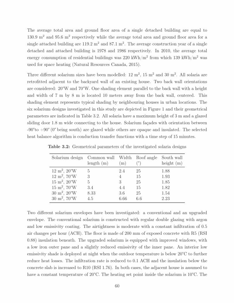
The average total area and ground floor area of a single detached building are equal to

130.9 m2 and 95.6 m2 respectively while the average total area and ground floor area for a

single attached building are 119.2 m2 and 87.1 m2. The average construction year of a single

detached and attached building is 1978 and 1986 respectively. In 2010, the average total

energy consumption of residential buildings was 220 kWh/m2 from which 139 kWh/m2 was

used for space heating (Natural Resources Canada, 2015).

Three different solarium sizes have been modelled: 12 m2, 15 m2 and 30 m2. All solaria are

retrofitted adjacent to the backyard wall of an existing house. Two back wall orientations

are considered: 20°W and 70°W. One shading element parallel to the back wall with a height

and width of 7 m by 8 m is located 10 meters away from the back wall, centered. This

shading element represents typical shading by neighbouring houses in urban locations. The

six solarium designs investigated in this study are depicted in Figure 1 and their geometrical

parameters are indicated in Table 3.2. All solaria have a maximum height of 3 m and a glazed

sliding door 1.8 m wide connecting to the house. Solarium façades with orientation between

-90°to +90° (0° being south) are glazed while others are opaque and insulated. The selected

heat balance algorithm is conduction transfer functions with a time step of 15 minutes.

Table 3.2: Geometrical parameters of the investigated solaria designs

Solarium design Common wall Width Roof angle South walllength (m) (m) (°) height (m)

12 m2, 20°W 5 2.4 25 1.8812 m2, 70°W 3 4 15 1.9315 m2, 20°W 5 3 25 1.8515 m2, 70°W 3.4 4.4 15 1.8230 m2, 20°W 8.33 3.6 25 1.5430 m2, 70°W 4.5 6.66 6.6 2.23

Two different solarium envelopes have been investigated: a conventional and an upgraded

envelope. The conventional solarium is constructed with regular double glazing with argon

and low emissivity coating. The airtightness is moderate with a constant infiltration of 0.5

air changes per hour (ACH). The floor is made of 200 mm of exposed concrete with R5 (RSI

0.88) insulation beneath. The upgraded solarium is equipped with improved windows, with

a low iron outer pane and a slightly reduced emissivity of the inner pane. An interior low

emissivity shade is deployed at night when the outdoor temperature is below 20°C to further

reduce heat losses. The infiltration rate is reduced to 0.1 ACH and the insulation below the

concrete slab is increased to R10 (RSI 1.76). In both cases, the adjacent house is assumed to

have a constant temperature of 20°C. The heating set point inside the solarium is 10°C. The

60

heating needs along with the excess heat inside the solarium when the temperature exceeds

28°C are presented in the next section.

Table 3.3: Solaria design characteristics

Conventional Upgraded

Conventional db glazing with argon\low-e Improved db glazing with argon\low-eConstant infiltration at 0.5 ACH Constant infiltration at 0.1 ACHR5 insulation below the floor R10 insulation below the floor

Low emissivity shade deployed at night

3.2.2 Commercial buildings

The total floor area and estimated ground floor area for commercial and institutional build-

ings in Québec are presented in Table 4. As indicated in the Commercial and Institutional

Building Energy Use Survey (Natural Resources Canada, 2002), the average number of storeys

of commercial and institutional buildings is equal to 2.70. Consequently, the total ground

floor area is estimated by dividing the total floor area by the average number of storey.

As presented in Natural Resources Canada (2002), the total floor area of commercial and

institutional buildings greater than 929 m2 was 63.6 km2 in 2000, or 89.4% of the total floor

area. Using this proportion and the more recent data presented in the 2008 Commercial &

Institutional Consumption of Energy Survey (Natural Resources Canada, 2008), the total

floor area of buildings greater than 929 m2 is estimated to 161.7 km2.

Table 3.4: Total floor area and ground floor area of commercial and institutional buildingsin Québec in 2008 adata from Natural Resources Canada (2008)

Building size Total floor area Total ground floor area

All 180.8 km2 a 67.0 km2

>929 m2 161.7 km2 59.9 km2

The average year of construction of commercial and institutional buildings in Québec is 1961

(Natural Resources Canada, 2002). In 2010, the average energy intensity was 462 kWh/m2

from which 171 kWh/m2 is consumed for space heating (Natural Resources Canada, 2015),

which is moderately higher than for residential buildings.

61

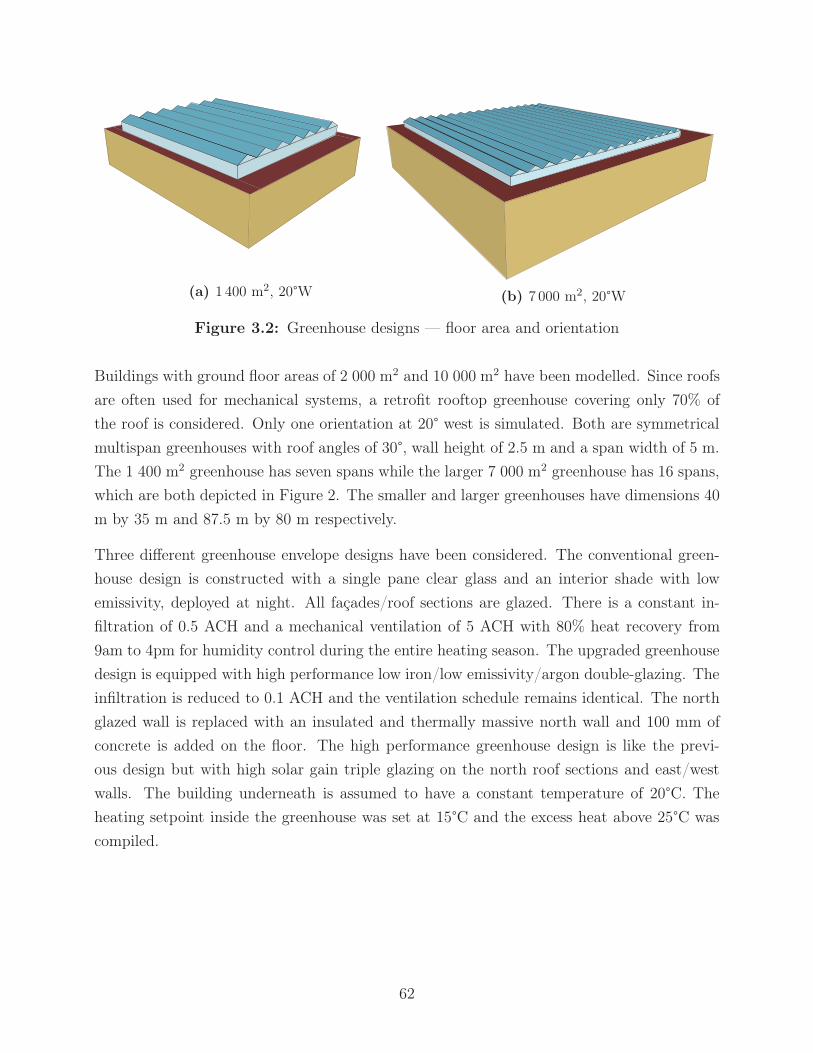
(a) 1 400 m2, 20°W (b) 7 000 m2, 20°W

Figure 3.2: Greenhouse designs — floor area and orientation

Buildings with ground floor areas of 2 000 m2 and 10 000 m2 have been modelled. Since roofs

are often used for mechanical systems, a retrofit rooftop greenhouse covering only 70% of

the roof is considered. Only one orientation at 20° west is simulated. Both are symmetrical

multispan greenhouses with roof angles of 30°, wall height of 2.5 m and a span width of 5 m.

The 1 400 m2 greenhouse has seven spans while the larger 7 000 m2 greenhouse has 16 spans,

which are both depicted in Figure 2. The smaller and larger greenhouses have dimensions 40

m by 35 m and 87.5 m by 80 m respectively.

Three different greenhouse envelope designs have been considered. The conventional green-

house design is constructed with a single pane clear glass and an interior shade with low

emissivity, deployed at night. All façades/roof sections are glazed. There is a constant in-

filtration of 0.5 ACH and a mechanical ventilation of 5 ACH with 80% heat recovery from

9am to 4pm for humidity control during the entire heating season. The upgraded greenhouse

design is equipped with high performance low iron/low emissivity/argon double-glazing. The

infiltration is reduced to 0.1 ACH and the ventilation schedule remains identical. The north

glazed wall is replaced with an insulated and thermally massive north wall and 100 mm of

concrete is added on the floor. The high performance greenhouse design is like the previ-

ous design but with high solar gain triple glazing on the north roof sections and east/west

walls. The building underneath is assumed to have a constant temperature of 20°C. The

heating setpoint inside the greenhouse was set at 15°C and the excess heat above 25°C was

compiled.

62

Table 3.5: Greenhouse design characteristics

Conventional Upgraded High performance

Fully glazed North wall replaced with an North wall replaced with aninsulated\massive north wall insulated\massive north wall

Single glass Db glass with argon\low-e Db on south, triple elsewhereLow-e interior shade Low-e interior shade Low-e interior shadeInfiltration 0.5 ACH Infiltration 0.1 ACH Infiltration 0.1 ACH

100 mm of concrete on floor 100 mm of concrete on floor

3.3 Results and discussion

3.3.1 Attached solaria

The heating needs, excess heat and net energy balance of the six case studies are presented in

Table 3.6. It can be seen that even conventional solaria can supply more useful heat than their

heating needs with a net energy balance of 28-75 kWh/m2 of solarium floor area. Upgraded

solaria are twice as efficient and can generate a net energy balance of 118-144 kWh/m2.

Table 3.6: Heating needs, excess heat and net energy balance of six solaria during theheating period

Design type Conventional Upgraded

Solarium Heating Excess Net energy Heating Excess Net energysize and needs heat balance needs heat balanceorientation kWh/m2 kWh/m2 kWh/m2 kWh/m2 kWh/m2 kWh/m2

12 m2, 20°W 33.2 108.4 75.3 15.7 158.3 142.612 m2, 70°W 32.9 100.2 67.3 13.3 147.5 134.315 m2, 20°W 36.9 94.3 57.5 10.3 154.5 144.115 m2, 70°W 31.0 86.4 55.4 11.5 131.3 119.830 m2, 20°W 29.5 82.0 52.5 5.5 141.9 136.430 m2, 70°W 37.2 64.8 27.6 5.2 123.0 117.8

It is interesting to compare the energy potential of solaria per floor area, which is between

28-144 kWh/m2, with the useful solar energy collected by water-based solar thermal panels

in Montreal, which is between 150-610 kWh/m2, depending on the size of the system (Wallin

et al., 2012). The wide variation of the energy performance of solaria indicates that careful

design and high quality materials must be selected in order to build a high performance

solarium with the capability of collecting significant amount of heat.

63

Considering an average single detached house in Québec with a total floor area of 130.9 m2

that adds an upgraded solarium, the heating consumption could be reduced by 1 612-4 092 kWh,

depending on the size and design of the solarium. This would reduce the average heating

requirements from 139 kWh/m2 down to 108-127 kWh/m2, a 9% to 23% reduction.

If 1% of all attached and detached houses in Québec would add an upgraded solarium, 31.3-

79.5 GWh of solar heat could be collected.

3.3.2 Rooftop greenhouses

The heating needs, excess heat and net energy balance of the two rooftop greenhouses studied

here are presented in Table 3.7. Large greenhouses used for the commercial production of

vegetables must have a thermally controlled indoor climate to support satisfactory crop

growth. A heating set point of 15 °C has been chosen for these simulations and the excess

heat was compiled for temperatures above 25 °C. It can be seen that conventional single

glazed greenhouses exhibit heating needs that exceed by far the excess heat that can be

collected with a net energy balance ranging from -298 to -321 kWh/m2.

Table 3.7: Heating needs, excess heat and net energy balance, in kWh/m2 of greenhousefloor area, of two rooftop greenhouses during the heating period

Design Conventional Upgraded High performance

Solarium Heating Excess Net Heating Excess Net Heating Excess Netsize and needs heat energy needs heat energy needs heat energyorientation balance balance balance

1 400 m2, 344.6 23.2 -321.4 73.2 70.4 -2.8 47.5 77.1 29.620°W7000 m2, 320.4 22.2 -298.2 66.3 67.3 -1.0 43.2 73.9 30.720°W

By increasing the airtightness, adding interior thermal mass and switching to high quality

double glazing, upgraded greenhouses can become fairly close to being net zero regarding

their heating consumption. In other words, upgraded greenhouses have the potential to

supply enough heat to adjacent buildings to compensate for their own heating consumption

throughout the year and thus have a net zero heating demand.

The thermal performance of greenhouses can be further improved by converting north, east

and west glazing to high solar heat gain low emissivity triple glass. Doing so allow generating

a positive net energy balance of about 30 kWh/m2. Adding a second thermal screen could be

64

more cost effective than selecting triple glazing and would add a lower weight. The use of two

thermal screens has not been modelled here due to the inability of EnergyPlus to simulate

two interior shading devices.

Covering 1% of large commercial and institutional buildings with rooftop greenhouses on 70%

of their roof area would create 0.42 km2 of cultivation area, enough to provide vegetables for

about 300,000 persons.

3.3.3 Discussion

As seen from the results presented above, the heating requirements of solaria and greenhouses

can exhibits large variations and are highly dependent on their design and operation. The

configurations studied here have not been optimized and it is thus possible to further improve

their net energy balance by doing so.

In this study, all excess heat during the heating season has been considered useful. Consid-

ering the low insulation levels and high heating requirements of the existing building stock,

assuming that all excess heat would be welcome at all times in adjacent buildings is reason-

able. However, for new buildings with a better envelope, this will likely not be the case and

a more detailed study considering the hourly heating demand and excess heat availability

would be required.

An Ideal Loads Air System has been selected for these simulations, which means that a 100%

efficient HVAC system was assumed. Heating and cooling set points were entered in the

Thermostat module. The ideal load assumption is realistic in the case of solaria heated with

small electric baseboards, but large greenhouses are likely to be equipped with a central

combustion heating system where in this case the actual efficiency of the heating system

should be taken into account. The total cooling energy for a given cooling set point was

interpreted in this study as the excess heat available for heating adjacent buildings during

the heating season.

For the solarium models, the distribution of the solar radiation on interior surfaces is modeled

by projecting the sun’s ray on interior surfaces, as described in details in U.S. Department

of Energy (2013) for the Full Interior and Exterior option. However, for the greenhouse

models, the Full Exterior option was selected where all beam solar radiation is assumed to

fall on the floor. This is a reasonable assumption in this case given the large surface of the

floor compared to that of the walls.

65

3.3.4 Conclusion

This chapter presented an analysis of the energy saving potential of attached solaria and

rooftop greenhouses for the province of Québec. Various realistic situations have been con-

sidered. A total of eighteen case studies have been simulated with the EnergyPlus building

simulation software. Six different solarium designs with different sizes and orientation have

been considered. Two rooftop greenhouse models with different sizes have also been simu-

lated.

For all cases, different building envelopes have been analysed. Results indicate that the

investigated solaria exhibit a net energy balance of 28-144 kWh/m2 of solarium floor area.

Retrofitting an upgraded solarium to an average house would reduce its heating consumption

by 1 612-4 092 kWh, depending on the size of the solarium, which corresponds to a 9% to

23% reduction. Retrofitting an upgraded solarium to 1% of all single detached and attached

houses in Québec would save 31.3-79.5 GWh annually.

Conventional greenhouses experience heating needs that far exceed their potential excess

heat contribution. However, with improved air tightness, thermal load levelling and high

quality double glass, net zero heating can be achieved. Surplus heat of up to 31 kWh/m2

of greenhouse floor area can be collected when using high performance triple glazing on the

northern, eastern and western orientations. Covering 1% of large commercial and institutional

buildings in Québec with rooftop greenhouses could provide enough vegetables to feed 300

000 people without increasing the total energy consumption of the province.

66

Chapter 4

Development of a solarium model

Different solarium models have been developed in Matlab. These models are described in

details in chapters 5, 6 and 7. This section presents the solar radiation models along with

the convective and radiative models that are used in the three chapters cited above. The

development of custom models was necessary because building simulation software currently

available do not offer the flexibility and feedback (about intermediate physical parameters of

interest) necessary to reach the objectives pursued in this thesis.

4.1 Solar radiation modelling

Commonly used equations for calculating the declination angle δ, the extraterrestrial radia-

tion flux Ion, the hour angle H , the solar altitude α and the solar azimuth angle φ can be

found in appendix C.

4.1.1 Solar radiation on sloped surfaces

This section presents the equations needed to calculate the direct and diffuse solar radiation

incident on a surface with an arbitrary orientation from weather data. Weather files for

energy calculations are available for hundreds of cities throughout the world. These weather

files typically report hourly values for the direct and diffuse (or global) solar radiation.

67

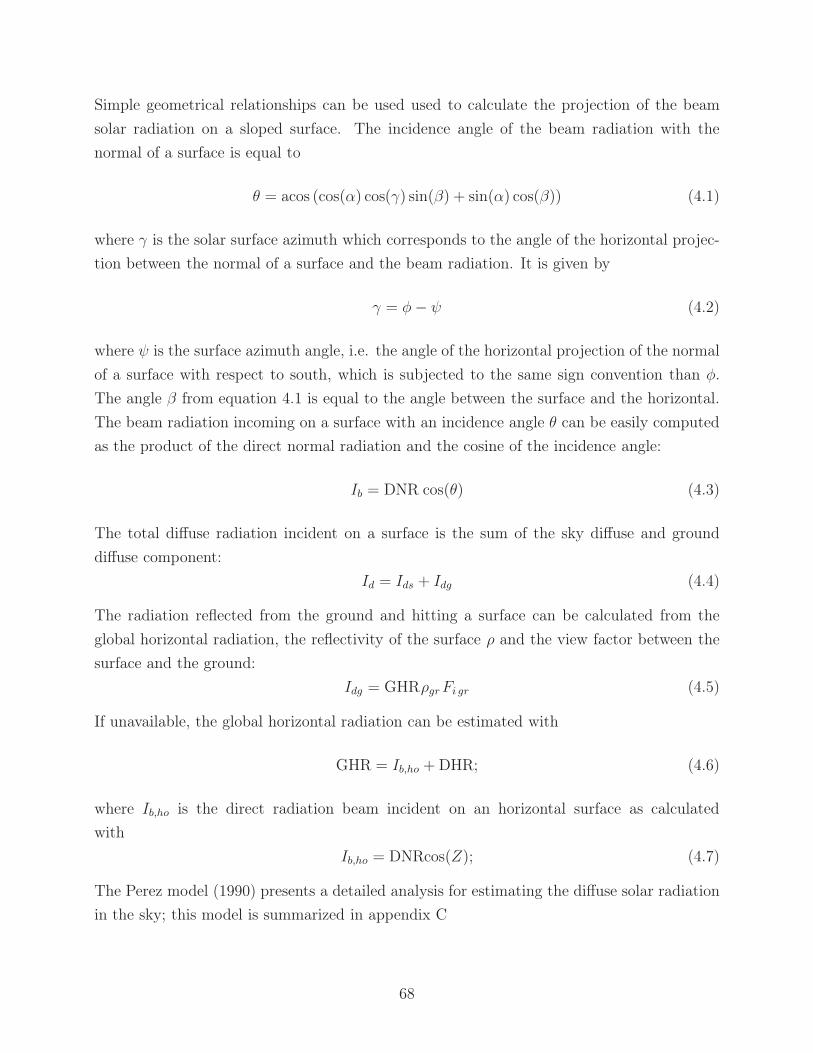
Simple geometrical relationships can be used used to calculate the projection of the beam

solar radiation on a sloped surface. The incidence angle of the beam radiation with the

normal of a surface is equal to

θ = acos (cos(α) cos(γ) sin(β) + sin(α) cos(β)) (4.1)

where γ is the solar surface azimuth which corresponds to the angle of the horizontal projec-

tion between the normal of a surface and the beam radiation. It is given by

γ = φ − ψ (4.2)

where ψ is the surface azimuth angle, i.e. the angle of the horizontal projection of the normal

of a surface with respect to south, which is subjected to the same sign convention than φ.

The angle β from equation 4.1 is equal to the angle between the surface and the horizontal.

The beam radiation incoming on a surface with an incidence angle θ can be easily computed

as the product of the direct normal radiation and the cosine of the incidence angle:

Ib = DNR cos(θ) (4.3)

The total diffuse radiation incident on a surface is the sum of the sky diffuse and ground

diffuse component:

Id = Ids + Idg (4.4)

The radiation reflected from the ground and hitting a surface can be calculated from the

global horizontal radiation, the reflectivity of the surface ρ and the view factor between the

surface and the ground:

Idg = GHRρgr Fi gr (4.5)

If unavailable, the global horizontal radiation can be estimated with

GHR = Ib,ho + DHR; (4.6)

where Ib,ho is the direct radiation beam incident on an horizontal surface as calculated

with

Ib,ho = DNRcos(Z); (4.7)

The Perez model (1990) presents a detailed analysis for estimating the diffuse solar radiation

in the sky; this model is summarized in appendix C

68

4.1.2 Solar radiation distribution on interior surfaces

In most building energy simulation software, all radiation transmitted through a window

is usually distributed on interior surfaces, while usually about 95% is actually retained in

a room. However, for highly glazed spaces, Wall (1995) has shown that only 30%-90% of

radiation transmitted through the glazing is retained in the space.

Wall (1997) also showed that simulation programs reveal important differences in the cal-

culation of solar gains in glazed spaces. Simpler simulation programs that do not calculate

accurately the solar radiation distribution overestimate significantly the absorbed solar ra-

diation. This emphasizes the importance of using a detailed method for the calculation of

solar radiation distribution in a highly glazed space.

In this model, the solar radiation transmitted through windows is distributed inside the so-

larium by combining ray tracing and radiosity methods. First, the transmitted beam solar

radiation is distributed on interior surfaces using ray tracing techniques by calculating the

area of a window illuminating directly a surface. The transmitted beam radiation directly

illuminating a portion of a surface is assumed to be uniformly distributed on that surface;

likewise, each surface is assumed to have a uniform temperature. The reflected component

is treated as diffuse and therefore distributed with a radiosity method, along with the trans-

mitted diffuse solar radiation.

A rectangular room with a south facing window is illustrated in Figure 4.1. It can be seen

that only up to three surfaces can be illuminated directly by a beam radiation. To find the

portion of the window illuminating a surface fw,i, the coordinates of that surface need to be

projected onto the window plane. fw,i is equal to the overlapping area between the window

and the image of the surface. For instance, to find the window area illuminating the back wall

fw,2, the back wall coordinates (ABCD) are projected along the sun’s ray into the window

plane (A′B′C′D′).

A point P(x,y,z) can be projected into the window plane to become point P′(x′,y′) by applying

the following transformation

x′ = x + z

(cos(θ2)

cos(θ1)

)(4.8)

y′ = y + z

(tan2(θ1) −

(cos(θ2)

cos(θ1)

)2)1/2

69

where θ1 is the angle of incidence in the plane z = 0 and θ2 is the angle of incidence on the

plane x = 0.

x

y

z

����������

����������

����������

����������

�����

�����

☼��������������������� B

A

C

D

E

O

B′

A′

C′

D′

fw,1

fw,2

fw,3

Figure 4.1: Projection of the backwall onto the window plane along a sun’s ray

Once the transformation of the coordinates is performed, the overlapping area between the

two polygons needs to be determined. A detailed method to compute the overlapping area

between convex polygons is presented in Walton (1979). Vertices defining the overlap between

two polygons A and B are either

• Vertices of A enclosed by B

• Vertices of B enclosed by A

• Intercepts of sides of A with sides of B

For a convex polygon with clockwise vertices, a point is enclosed in this polygon if it lies to

the right of all sides of the polygon. For a counterclockwise polygon, a point is enclosed in

the polygon if it lies to the left of all its sides. This can be determined by calculating a scalar

product. Let’s consider a point (x, y) represented by a three elements vector (x, y, 1) and a

line represented by a three elements vector (a, b, c). If (a, b, c) · (x, y, 1) > 0, the point lies to

the left of the line; similarly, if (a, b, c) · (x, y, 1) < 0, the point is to the right of the line.

70

Figure 4.2: Two overlapping polygons

The intercept of lines (a1, b1, c1) and (a2, b2, c2) can be found with (a1, b1, c1) × (a2, b2, c2).

However, before calculating their intercept, it should be determined if the lines intercept

within their end points. Two line segments A and B intercepts if the ends of A lies to both

sides of B and the ends of B lies to both sides of A. If this is the case, the dot product between

line A and the two end points of B will have different signs, as well as the dot product of line

B with the end points of A. Additional details on the calculation of vertices of overlapping

polygons can be found in Walton (1979).

���������

����

����

���

����������

�����

������

�������

a) b) c)

Figure 4.3: Line segments

Once the vertices of the overlapped polygon are known, fw,i can then be computed. The solar

radiation absorbed by interior surfaces in the room is calculated following the procedure

presented in Athienitis and Sullivan (1985) and Athienitis and Stylianou (1991). The total

beam radiation absorbed by a surface i is given by

Sb,i = αiGbfw,i + Ai

∑j

F dij ρj Gbfw,j

Aj(4.9)

where αi is the absorptance of surface i, Gb the transmitted beam radiation, Ai is the area of

surface i, F dij is the transfer factor and ρj is the reflectance of surface j. The transfer factor

F dij is the fraction of diffuse solar radiation emitted by surface j which is absorbed by surface

i and is calculated with

F dij = AFik M−1

kj (4.10)

71

where A is a diagonal matrix with the surfaces absorptance equal to its diagonal, Fik is the

view factor and M−1kj is the inverse of the matrix Mkj which is given by

Mkj = Ikj − ρk Fkj (4.11)

with I being an identity matrix. Note that the first term of equation (4.9) represents the

beam radiation absorbed directly by surface i while the second term represents the beam

radiation absorbed as diffuse radiation after many reflections. The diffuse solar radiation

transmitted through a window and absorbed by surface i is calculated with

Sd,i = AiGdF diw (4.12)

For the case of the window, one more term should be added to take into account the incoming

radiation directly absorbed by the window

Sd,w = Aw GdF dww + Aw Ga (4.13)

where Ga represents the incoming radiation absorbed in the glazing.

4.2 Convective heat transfer coefficients

The heat exchanged by convection between a surface i and the air is expressed as

Q = Ai hc (Tin − Ti) (4.14)

where hc is a convective coefficient. The convective heat transfer between a surface and the

air depends mainly on the position of the surface (horizontal/vertical) and the temperature

difference between the surface and the air. Many correlations have been developed to charac-

terize natural, mixed or forced convection. For an interior surface in a room, the air velocity

is relatively low and therefore correlations for natural convection may be employed. Khalifa

and Marshall (1990) developed correlations for the calculation of the heat transfer convec-

tive coefficient of interior building surfaces. They found that for a vertical glazing (with no

radiator under the window), a vertical wall and an horizontal surface (facing upward), the

convective heat transfer coefficient may be estimated with

72

Vertical glazing hc = 7.61(ΔT )0.06 (4.15)

Vertical wall hc = 2.03(ΔT )0.14 (4.16)

Horizontal surface hc = 2.27(ΔT )0.24 (4.17)

where ΔT is the temperature difference between the surface and the air. The convective

coefficient representing the effect of wind on the exterior surface of a building is calculated

with (Duffie and Beckman, 2006)

hc,w =8.6v0.6

w

L0.4(4.18)

where L is the cube root of the solarium volume. Convective coefficients for air spaces

between window panes and between windows and shading devices are calculated following

the procedure outlined in ISO 15099 (2003) for thermally driven ventilation. The convective

coefficient in a ventilated gap is given by

hc,v = 2hc,nv + 4vmean (4.19)

where hc,nv is the convective coefficient for non-vented cavities. A pressure-balance equation

is used to determine the mean air velocity in the cavity and other variables of interest like

the outlet air temperature in the gap. The heat balance equations are solved iteratively until

they converge. The mean air velocity in the cavity is determined from

vmean =

[(12νρHg

L2

)2

+2ρ(1 + Zin + Zout)ρoTogHg sin β |Tgap,in − Tgap|

Tgap,inTgap

]1/2

− 12νρHg

L2

ρ(1 + Zin + Zout)(4.20)

where ν is the kinematic viscosity, Hg is the height of the glazing, L is the cavity width, Zin

and Zout are the inlet and outlet pressure drop factors, β is the angle between the glazing and

the horizontal, Tgap,in is the gap inlet temperature, Tgap is the mean gap air temperature, the

subscript o refers to a glazing height of zero and other symbols were previously defined.

Equations for calculating hc,nv, Zin, Zout and Tgap and details about the iteration procedure

are given in the Engineering Reference documentation of EnergyPlus (U.S. Department of

Energy, 2013) and in ISO 15099 (2003). The equation for vmean contains an error in the

EnergyPlus reference; the equation above has been corrected.

73

4.3 Radiative heat transfer models

Long wave radiation exchanges between interior surfaces can be modeled using the Gebhart

method (Gebhart, 1959; Siegel and Howell, 1981; Mottard and Fissore, 2007). In this case,

the net radiation flux emitted by a surface i is calculated as

qLWR,i = −εiAiσ

n∑j=1

Gij

(T 4

i − T 4j

)(4.21)

where n is the number of surfaces and Gij is a Gebhart coefficient. The sign is negative

because the flux is leaving the surface. The n2 Gebhart coefficients, which depend on the

geometry and thermal properties of the surfaces, can be obtained by solving

⎛⎜⎜⎜⎜⎝

(1 − ρ1F11) −ρ2F12 − · · · −ρnF1n

−ρ1F21 (1 − ρ2F22) − · · · −ρnF2n

− · · · − · · · . . . − · · ·−ρ1Fm1 −ρ2Fm2 − · · · (1 − ρnFmn)

⎞⎟⎟⎟⎟⎠

⎛⎜⎜⎜⎜⎝

G1k

G2k

...

Gnk

⎞⎟⎟⎟⎟⎠ =

⎛⎜⎜⎜⎜⎝

F1kεk

F2kεk

...

Fnkεk

⎞⎟⎟⎟⎟⎠ (4.22)

Longwave radiation exchange between an exterior surface and the ground, sky and air is

calculated with

qLWR,o = Ai

(hr,gnd (Tgnd − Ti) + hr,sky (Tsky − Ti) + hr,air (To − Ti)

)(4.23)

where the sky temperature is calculated from the atmospheric temperature (ASHRAE, 2007)

and the ground temperature is assumed to be the same as the air temperature. The linearized

radiative coefficients are calculated as

hr,gnd =εσFgnd(T

4i − T 4

o )

Ti − To

(4.24a)

hr,sky =εσFsky(T

4i − T 4

sky)

Ti − Tsky(4.24b)

hr,air =εσFair(T

4i − T 4

o )

Ti − To

(4.24c)

Radiative heat transfer between panes of glass and window/shade cavities are calculated

based on the fundamental equation for two infinite parallel plates

qLWR,1→2 =Aiσ

(T 4

2 − T 41

)1

ε1+

1

ε2− 1

(4.25)

74

Chapter 5

Methodology for selecting fenestration

systems in heating dominated climates

Based on a published paper:

Bastien, D. and Athienitis, A. 2015a. Methodology for selecting fenestration systems in

heating dominated climates. Applied Energy, 154, 1004-1019.

5.1 Chapter abstract

Selecting optimum windows in heating dominated climates is a complex task because of the

inherent trade-off between their U-value and solar heat gain coefficient. In addition, the use

of shades is known to reduce heat losses, but they are rarely selected for this intent and

considered as an integrated fenestration system at the design stage. This paper presents a

method for selecting optimum fenestration systems (windows with shades) to maximize the

annual net energy balance. The method has the capability to simulate a one or two layer

shading system with one exterior and/or one interior planar shade(s). This methodology

generates 2D schematics indicating the net energy balance of different fenestration systems.

Such schematics are useful at an early design stage when there is a need to compare different

design options for different orientations on a relative basis.

Diagrams are presented for five glazings with an interior roller shade, an exterior roller shutter

and a combination of both, for the four cardinal orientations for the city of Montreal, Canada.

A comparison of simulated and experimental U-values of four shading devices indicates results

reasonably close to each other.

75

5.2 Introduction

With increasing awareness to climate change and sustainable development, many studies have

been conducted on improving the energy efficiency of buildings due to their important energy

consumption. Indeed, in Canada, the energy consumed by the residential and commercial

sectors represented 29% of the total energy use in 2012 (Natural Resources Canada, 2015),

most of which used by buildings.

Virtually all previous research agree on the importance of windows and shading systems on

the energy consumption of buildings (Tzempelikos et al., 2007; Ochoa et al., 2012; Lee et al.,

2013; Koo et al., 2014; Huang et al., 2014; Hee et al., 2015). For instance, a Canadian study

on high-rise residential buildings has reported that windows were responsible for an average

of 31% of total energy loss (CMHC, 1996).

Selecting optimal windows is more complicated than opaque envelope components since the

performance of windows is governed by two major variables: the solar heat gain coefficient

(SHGC) and the thermal resistance. In cold climates, it is desirable to have windows with

both high thermal resistance and SHGC so as to optimize utilization of solar gains. The

resistance of a window may be increased by adding a supplementary pane of glass, applying

a low emissivity coating and using an inert gas such as argon or krypton in the cavity.

However, the former two options also reduce the SHGC, which could lead to an increased

heating demand. In addition, windows are one the most expensive component in a house (on

a unit area basis). As a result, the selection of windows (and their area) is one of the most

problematic aspect of Net-Zero Energy Buildings (Proskiw, 2010).

Windows with different orientations are not affected by these two variables to the same

extent: an equatorial-facing window (referred to as south facing in the rest of the paper) will

have a better performance with a high SHGC while it is more beneficial for a north window

to have a lower U-value (Karlsson and Roos, 2001). Thus selecting different windows for

different orientations could reduce the energy consumption of buildings.

Moreover, the use of shading devices, and their operation if moveable, affects the performance

of windows, altering their thermal performance and solar gains. An extensive study of various

window attachments estimated through simulations that simple shading devices like interior

roller shades and exterior solar screens could improve the U-value of a double glazed low

emissivity window by 3-45% and 26-39% respectively, depending on the characteristics of the

shading device (Curcija et al., 2013).

76

5.2.1 Background

For improving the performance of façades, it has been suggested to divide the window area

into two parts: the daylighting section at the top and the view section below. Since glazing

below the workplane does not contribute significantly to daylighting and is detrimental for

the building energy consumption (Schumman et al., 2013), this section is better opaque, thus

creating a three-section façade concept as described by Tzempelikos (2005) where ideally

the view section provides diffuse light only. Schumman et al. (2013) suggested to use high

transmission glass at the upper section and lower transmission glass in the view section for

controlling glare, with additional forms of solar control for both sections. Tzempelikos et al.

(2007) suggested to use automated venetian blinds for the upper part and manually controlled

roller shade for the lower part of the window for high daylight autonomy and comfort and

low energy consumption.

As noted by Tzempelikos and Athienitis (2007), cooling may be important in perimeter zones

even in heating dominated climates, indicating that shading is a necessity. Because of the

importance of shading devices on the performance of buildings, a few general recommenda-

tions will be reported here. For additional guidelines regarding shading strategies, one may

refer to Schumman et al. (2013).

Shading type and properties should vary with orientation, since their performance indices

are very sensitive to this variable (Tzempelikos and Athienitis, 2007).

Exterior shading is more effective than interior shading for blocking solar gains. Interior

shading devices should be light-coloured to better reflect solar radiation. For exterior shading

devices, horizontal forms should be preferred for a south façade, such as overhangs and

awnings, while vertical forms should be preferred for a east, west and north façades, such as

vertical fins. It is also good practice to have different shading solutions that can be managed

independently for the view and daylight sections (Schumman et al., 2013).

Ochoa et al. (2012) have found that east and west windows have the highest energy consump-

tion, Lee et al. (2013) have noted that the energy performance of east and west windows being

more sensitive to changes in SHGC and visible transmittance and Huang et al. (2014) have

identified east and west orientations as having the most potential for reducing the energy

consumption of a building using shading devices. These observations indicate that special

care must be taken when designing east and west windows and their protections.

77

Nielsen et al. (2011) noted that north windows with no shadings or fixed shadings are a

relevant alternative, but suggests the use of automated venetian blinds for improving the

daylight availability of large windows of other orientations.

Since shading devices play an important role in the energy performance of buildings, some

tools have been developed to facilitate the task of selecting windows and window-shade

systems (the latter being referred to as fenestration systems throughout this study).

5.2.2 Existing tools and research needs

Many tools already exist to help selecting windows and fenestration systems. Programs such

as WINDOW (and its companion software THERM and RESFEN) (LBNL, 2014, 2005), WIS

(WinDat, 2004) and ParaSol (Lund University, 2010) are stand-alone tools that calculate

the solar and thermal properties of windows, which may be accompanied with some types of

shading devices. WINDOW and WIS are mainly used for certification purposes as they carry

out simulations at fixed conditions, usually chosen to match a specific standard. RESFEN

and ParaSol offer the possibility of calculating annual heating and cooling loads associated

with windows. There are also whole building energy simulation software with the capability

of carrying detailed heat transfer calculations through windows and fenestration systems like

EnergyPlus (U.S. Department of Energy, 2013), TRNSYS (Klein and al., 2010) and ESP-r

(ESR U, 2011). A more detailed description of these software can be found in (Loutzenhiser

et al., 2007), (Tzempelikos, 2008) and in (Rogalsky, 2011).

Nielsen et al. (2001) presented a method for comparing the energy performance of glazings or

windows for heating dominated buildings. The net energy gain is calculated for the heating

season and is equal to the solar gains minus the heat losses through the glazing. Following

this method, diagrams presenting the net energy gain for different combinations of SHGC

and U-values are generated for a specific orientation. These diagrams are useful since they

allow to quickly visualize what is the optimum window for a given orientation. Heat gains

can be reduced by employing a shading coefficient to represent overhangs or obstructions,

but only a fixed value for the year can be simulated. This simple method can be used either

with glazings or whole windows, but cannot evaluate the impact of shading devices.

For achieving low energy buildings with satisfactory indoor climate, the designers have to be

aware as early as possible of the consequences of critical design decisions (Hviid et al., 2008).

Tools with simplified input are needed for supporting decisions in the early design stages of

a building (Nielsen, 2005).

78

The most accurate way of analyzing the performance of windows and shading devices is with

detailed dynamic energy building simulations for a specific building and climate (Tzempelikos

and Athienitis, 2007). Lee et al. (2013), among others, have identified different optimal

window properties in different climates and different optimal window properties for different

orientations in the same location. These results emphasize the need of evaluating different

window properties when designing energy efficient buildings. However, analyzing multiple

coupled variables such window size and type, shading type, properties and control, for all

four orientations of a building can yield to a very large solution space.

One way to reduce the solution space of whole building simulations is to first use single space

models to identify optimum shade designs and then analyze the identified optimums with

whole building simulations, an approach followed by Orsi (2009).

As an alternative, the methodology described in this paper can be used first to identify

optimum glazing and shading combinations as a function of orientation before carrying whole

building simulations. Once implemented, the proposed methodology can be readily used at

the design stage for a new project and requires significantly less effort that developing new

single space building models.

5.2.3 Objectives and overview

After reviewing the existing tools, it can be seen that there is a need to develop a simple tool

to be used at the preliminary design stage allowing the comparison of the net energy balance

of various fenestration systems. The influence of the shades on the SHGC and U-value of the

fenestration system must be accounted for in the energy balance. In addition, the control of

shades should be customizable.

The goal of this paper is to present a methodology for selecting optimum fenestration systems.

It has the capability of calculating the net energy gain of windows with one interior and/or

one exterior shade(s), which covers most important cases. This methodology can be used

independently or as an early stage design tool for identifying fenestration systems with the

best performance before running whole building simulations.

The section 5.3 below presents the methodology for comparing the net energy balance of un-

shaded glazings, glazings with an exterior shade, glazings with an interior shade and glazings

with both interior and exterior shades. It is based from (Nielsen et al., 2001), where some

modifications were introduced to increase its accuracy and where the capability of analyzing

shades has been integrated. Applications and limitations of this methodology are detailed

79

in section 5.4 along with some recommendations. Results are then presented in section 5.5,

where diagrams for glazings with an interior roller shade, an exterior roller shutter and a

combination of both are presented for the four cardinal orientations for the city of Montreal.

Finally, section 5.6 presents a comparison of experimental and simulated U-values for four

types of shading devices.

The methodology presented in this paper can be used for comparing either glazings or

complete windows. For clarity, equations are presented for glazings only throughout this

paper. Appendix 5.3.3 describes how to adapt the calculations for investigating complete

windows.

5.3 Methodology for selecting fenestration systems

Canadian Weather for Energy Calculations (CWEC) files were used for this study. Any

hourly weather data freely available on the U.S. Department of Energy (2015) website can be

downloaded and serve as input. The inputs required are the time and day of the year, out-

door temperature, global horizontal radiation, direct normal radiation and diffuse horizontal

radiation.

5.3.1 Unshaded glazings

5.3.1.1 Calculating net energy gain

The net energy gain (or loss) through a glazing or a window is calculated as

Q = SHGC · I − U · D (5.1)

where SHGC and U are the solar heat gain coefficient and U-value of the glazing or window

and I and D are given as

I = ηFs

∑t

(Ib gj(θ)Δt′ + IdfjΔt′

)for To < Tb (5.2)

D =∑

t

(Ti − To)Δt′ for To < Tb (5.3)

80

Ib and Id are given in section 4.1.1 where the sky diffuse radiation is modeled with the Perez

model (Perez et al., 1990). The angular profile gj is used to approximate the dependency of

the SHGC to the incidence angle. fj represents the ratio of the SHGC for diffuse radiation

to the SHGC at normal incidence. It is calculated with (Finlayson et al., 1993)

fj = 2

∫ π/2

0

gj(θ)sin(θ)cos(θ) (5.4)

fj and gj are provided in table 5.1 as a function of the number of panes j. Although the

angular profiles have been determined for clear glass, they have shown a mean average error

of 1% and a maximum error of 5% when used with a variety of coated glass (Karlsson et al.,

2001). A more detailed polynomial method presented in the work cited above can be used if

a higher accuracy is required.

Table 5.1: Angular profiles, from Karlsson et al. (2001)

θ g1 g2 g3

0 1 1 15 0.9999 0.9998 0.999710 0.9994 0.9992 0.998915 0.9987 0.9980 0.997520 0.9975 0.9962 0.995425 0.9956 0.9936 0.992430 0.9928 0.9897 0.988235 0.9886 0.9841 0.982540 0.9823 0.9758 0.974345 0.9728 0.9636 0.962250 0.9585 0.9450 0.943655 0.9368 0.9162 0.913260 0.9034 0.8710 0.862565 0.8522 0.8003 0.778970 0.7740 0.6927 0.650775 0.6564 0.5412 0.479680 0.4865 0.3537 0.290585 0.2597 0.1592 0.120990 0 0 0

f1 f2 f3Hemispherical 0.9114 0.8854 0.8748

Tin from equation 5.3 is the average interior temperature during the heating season. Equa-

tions 5.2 and 5.3 are computed only when the outdoor temperature To is below the balance

temperature Tb. The balance temperature is usually defined as the value of the outdoor tem-

perature when the internal and solar gains are equal to the building heat losses (ASHRAE,

2009, Chapter 19). However, the solar gains are actually useful for eliminating heating needs81

and thus their contributions should be accounted for here. Therefore, the balance tempera-

ture used here should consider internal gains only and can be calculated from

Q = UAe(Tin − Tb) (5.5)

where here U is the overall building U-value, including infiltration and Ae is the total building

envelope area. For residential buildings, the internal gains (in W) can be estimated with

(ASHRAE, 2009, Chapter 17)

Q = 136 + 2.2Afloor + 22Noc (5.6)

The balance temperature could be 1 °C lower than Tin for old houses with little insulation

while it could be 5 °C lower for highly insulated houses like passive houses. For non-residential

buildings, internal gains should be determined accordingly to the expected building occu-

pancy and equipment. One may refer to ASHRAE (2009, Chapter 18) for more details.

To avoid considering useful heat gains in the hot season when no heating is used, equations

5.2 and 5.3 should be computed only during the heating season and transitional periods.

Fs in equation 5.2 represents a shading factor. This factor represents shading from distant ob-

jects, window reveals and fixed exterior shadings. It is possible to use a fixed value throughout

the year, or, as an alternative, monthly shading factors for various types of external shading

elements can be obtained with ParaSol (Lund University, 2010). 1

The value of the utilization factor η in equation 5.2 should be very close to 1. This method

is intended for buildings in heating dominated climates aiming at a high solar utilization,

in which case the solar gains as calculated with equation 5.2 are practically always useful.

Please refer to section 6.6 for further details about the applications and limitations of this

methodology.

5.3.1.2 Generating net energy gain diagram

Equations 6.6, 5.2 and 5.3 are then used to generate lines of constant energy gains or losses.

First, an array of energy gains (or losses) is defined, in kWh/m2 of window area. For in-

stance, in figure 5.1, Q is an array between -300 and 500 kWh/m2 with an increment of 50

kWh/m2.

1In this software, the f(g) output variable represents the shading factor of the obstruction under con-sideration. The graphical output can be easily exported to a text file and then imported for use with thismethodology.

82

Secondly, an array of possible SHGC must also be defined. Then, the user must deter-

mine the number of panes he is primarily interested in, for comparison purposes. Using the

corresponding corrected incident solar radiation I, from equation 5.2, an array of U-values

required to achieve a specific energy performance is calculated from isolating U in equation

6.6. Plotting the SHGC array as a function of these U-values generates a diagram with lines

of constant net energy gains (or losses).

U (W/m2-K)

SHG

C

Net energy gains (kWh/m2)

TR-ARar-2low-e

DBar-1low-e

DB-ARar-1low-e

DBar-2low-e

HM88

DBclear

-300-250-200-150-100-500

50

100

150

200

250

300

350

400

450

500

0 0.5 1 1.5 2 2.5 30

0.1

0.2

0.3

0.4

0.5

0.6

0.7

0.8

0.9

Figure 5.1: Net energy gains (in kWh/m2) of six glazings for a south orientation inMontreal during the heating period ranging from 15/09 to 15/05 with Fs=0.9, η=1 andTb=20°C. DB=Double; TR=Triple; AR=antireflective coating; ar=argon; low-e=low emis-sivity; HM88=DB glazing with suspended low-e plastic film.

After entering the U-value and SHGC of a few glazings of interest, their performance can

then be easily compared for a given orientation. Figure 5.1 shows the performance of six

different glazings on a south façade in Montreal.

The corrected incident radiation for single, double and triple glazings is presented in table

5.2 for Montreal for the conditions described in figure 5.1. The constant net energy gain

lines in this figure have been calculated for a double glazing. Although both double and

triple window products are depicted on the figure, it can be seen from table 5.2 that the

difference between the corrected incident radiation for single and double glazing is 2.2% and

for double and triple glazing is less than 1%. Therefore, it is possible to compare glazings

with a different number of panes on the same graphic with a reasonable accuracy.

83

Table 5.2: Corrected incident solar radiation for a single, double and triple glazing

I1 I2 I3

621 kWh/m2 607 kWh/m2 602 kWh/m2

5.3.2 Glazings with shading devices

The shade is assumed to cover the glazing only. Single, double and triple glazings can be

analyzed with the presence of an exterior or interior shade, or a combination of both.

The required inputs for glazings and shades are summarized in table 5.3. Ideally, the solar

transmittance and absorptance of window panes should be known. However, as an alternative,

this paper presents tables to estimate these values for single, double and triple glazing where

only the composition of the gas infill is required. In rare cases, if the emissivity of the

outermost or innermost pane is different than 0.84, then it should be specified.

Shades can be controlled based on a hourly schedule, a solar radiation set point or on more

detailed conditions determined by the user. It is also possible to use another program to

perform a more complete thermal analysis to determine an annual operation schedule and

import it into this methodology.

Table 5.3: Inputs parameters (aoptional, for the analysis of windows only)

Glazing

U-valueSHGCSolar transmittance and absorptances OR Gas infill and nb of panesEmissivity of outermost and innermost panes, if �= 0.84Height and width of glazing (or window*)Window U-valuea

Window areaa

Shade

Emissivity of both sides (typically ≈ 0.9)Thermal resistance OR thermal conductivity and thicknessSolar absorptanceSolar transmittanceSolar reflectance of the window facing sideCavity width between the shade and the windowOpenness factorTop/bottom/left/right opening area between the shade and glass

84

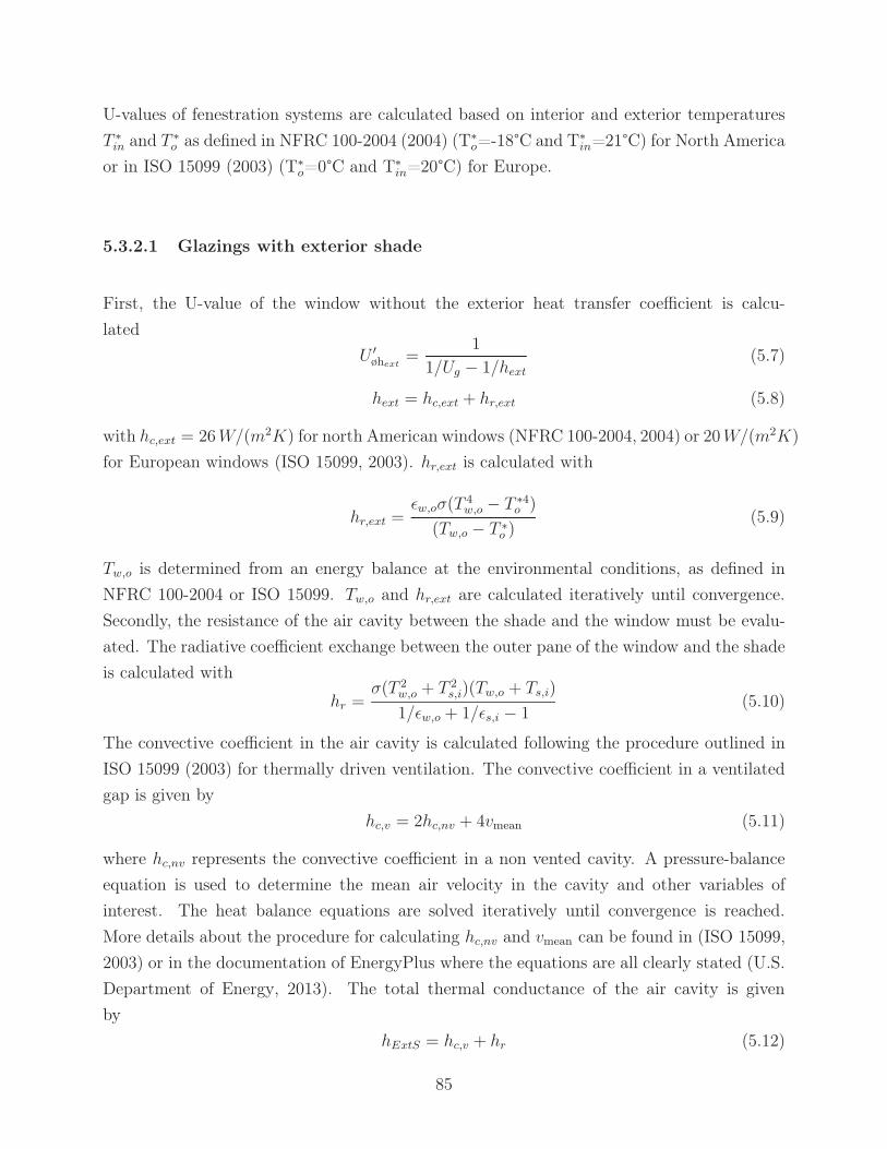
U-values of fenestration systems are calculated based on interior and exterior temperatures

T ∗in and T ∗o as defined in NFRC 100-2004 (2004) (T∗o=-18°C and T∗in=21°C) for North America

or in ISO 15099 (2003) (T∗o=0°C and T∗in=20°C) for Europe.

5.3.2.1 Glazings with exterior shade

First, the U-value of the window without the exterior heat transfer coefficient is calcu-

lated

U ′øhext=

1

1/Ug − 1/hext(5.7)

hext = hc,ext + hr,ext (5.8)

with hc,ext = 26 W/(m2K) for north American windows (NFRC 100-2004, 2004) or 20 W/(m2K)

for European windows (ISO 15099, 2003). hr,ext is calculated with

hr,ext =εw,oσ(T 4

w,o − T ∗4o )

(Tw,o − T ∗o )(5.9)

Tw,o is determined from an energy balance at the environmental conditions, as defined in

NFRC 100-2004 or ISO 15099. Tw,o and hr,ext are calculated iteratively until convergence.

Secondly, the resistance of the air cavity between the shade and the window must be evalu-

ated. The radiative coefficient exchange between the outer pane of the window and the shade

is calculated with

hr =σ(T 2

w,o + T 2s,i)(Tw,o + Ts,i)

1/εw,o + 1/εs,i − 1(5.10)

The convective coefficient in the air cavity is calculated following the procedure outlined in

ISO 15099 (2003) for thermally driven ventilation. The convective coefficient in a ventilated

gap is given by

hc,v = 2hc,nv + 4vmean (5.11)

where hc,nv represents the convective coefficient in a non vented cavity. A pressure-balance

equation is used to determine the mean air velocity in the cavity and other variables of

interest. The heat balance equations are solved iteratively until convergence is reached.

More details about the procedure for calculating hc,nv and vmean can be found in (ISO 15099,

2003) or in the documentation of EnergyPlus where the equations are all clearly stated (U.S.

Department of Energy, 2013). The total thermal conductance of the air cavity is given

by

hExtS = hc,v + hr (5.12)

85

The exterior radiative coefficient hr,ext must be recalculated based on the temperature of the

shade. The exterior convective coefficient hc,ext remains unchanged. Because the calcula-

tion of the radiative coefficient depends on the temperature of the surfaces, energy balance

equations must be solved iteratively until convergence is reached. The U-value of the whole

fenestration system is finally calculated as

UExtS =1

1/U ′øhext+ 1/hExtS + RExtS + 1/hext

(5.13)

Figure 5.2 summarizes the process for calculating the equivalent U-value. The net energy

gain must be calculated hourly taking into account if the shade is present or not:

if shade is absent

Q′t = SHGCgIj − Ug

(Tin − To

)U ′t = Ug

else

Q′t = SHGCExtS Ij − UExtS

(Tin − To

)U ′t = UExtS (5.14)

Figure 5.2: Flow chart for calculating the equivalent U-value of a fenestration system withan exterior shade. The ovals indicate that calculations are made iteratively until convergenceis reached.

86

The effective U-value of the fenestration system is simply the average of U ′t and the net energy

gain is the hourly sum of Q′t

Ueff = avg(U ′t) (5.15)

Q =∑

t

Q′t (5.16)

The effective solar heat gain is calculated with

SHGCeff =(Q + UeffD)

I(5.17)

where I and D are calculated from equations 5.2 and 5.3. Situating (Ueff,SHGCeff) on a

net energy gain diagram will indicate the net energy balance of the investigated fenestration

system. Note that SHGCeff is used only to situate the net energy balance Q on the graph.

While it gives an indication about how the shade and its control are reducing the equivalent

solar heat gain of a fenestration system, it has no explicit physical meaning. Under some

circumstances, its value can be above the SHGC at normal incidence of a bare window.

The presence of a shade affects not only the U-value of a fenestration system but also itsSHGC. The SHGC of a fenestration system depends on the solar transmittance and absorp-tance of the different layers (ISO 15099, 2003):

SHGC1g = τ + α1U

hext(5.18a)

SHGC2g = τ + α1U

hext+ α2

(hint − U)

hint(5.18b)

SHGC3g = τ + α1U

hext+ α2U

(1

hext+

1

Λ12

)+ α3

(hint − U)

hint(5.18c)

SHGC4g = τ + α1U

hext+ α2U

(1

hext+

1

Λ12

)+ α3U

(1

hext+

1

Λ12+

1

Λ23

)+ α4

(hint − U)

hint(5.18d)

where Λij represents the thermal conductance of the cavity between elements i and j, as

depicted in figure 5.3. The thermal resistance of the glass is always very small and therefore

neglected, but the thermal resistance of the shade is accounted for since it could be significant

in some cases. Layers are numbered with #1 being the outermost layer.

It is assumed that the dependency of the SHGC of the shading material with the incidence

angle is identical as the glazing under investigation. This assumption seems reasonable

especially with some shading materials like roller shades and insect screens where the analysis

of their beam total transmittance was shown to exhibit a similar trend than glass (Kotey

et al., 2009b,d). The total transmittance of a glazing with an outer shade is calculated

with

87

(a) Triple glazing (b) Double glazing with exterior and interior shades

Figure 5.3: Illustration of the thermal conductances Λij for different configurations

τExtS =τsτg

1 − ρ′sρg

(5.19)

Glazings, either single, double or triple, are considered as a single element with their solar

transmittance estimated with tables A.1 - A.3 if actual data is not available. The prime

in equation 5.19 refers to the spectral reflectance measured in the opposite direction of the

incident solar radiation. The typical solar reflectance of uncoated glass is 0.08.

As seen in equations 5.18, calculating the SHGC of a window with a shade requires the knowl-

edge of the solar transmittance and absorptance of the window panes. Ideally, they should

be specified as input. As an alternative, a simple method estimating the solar transmittance

and absorptances of a glazing from its U-value, SHGC and gas infill has been developed and

is presented in tables A.1, A.2 and A.3 in Appendix A. The absolute average and maximum

associated errors and shown in table A.4.

The total SHGC of a fenestration system that consists of an outer shade and a single, doubleor triple glazing is calculated with

SHGC1gExtS =τExtS + αsUExtS

hext+ τExtSαg

(hint − UExtS)

hint(5.20a)

SHGC2gExtS =τExtS + αsUExtS

hext+ τExtSαg1UExtS

(1

hext+

1

hExtS + 1/RExtS

)

+ τExtSαg2(hint − UExtS)

hint(5.20b)

SHGC3gExtS =τExtS + UExtSαs + τExtSαg1 + τExtSαg2 + τExtSαg3

hext

+ UExtSτExtSαg1 + τExtSαg2 + τExtSαg3

(1/hExtS + RExtS)−1

+ UExtSτExtSαg2 + τExtSαg3

Λ23+ UExtS

τExtSαg3

Λ34(5.20c)

88

In the case of a triple glazing with an exterior shade, the insulating value of the glass cavities,

Λ23 and Λ34, should be known to determine the SHGC of the fenestration system. This would

require the knowledge of the emissivity of panes #2, #3 #4 and #5 as well as the cavity

thicknesses and gas infill. If this information is known, Λ23 and Λ34 can be calculated using

equation 3 from ISO 10292 (1994). Alternatively, they can be approximated with

Λ23 = Λ34 =1(

1Ug

− 1hext

− 1hint

)/2

(5.21)

where hext is calculated using equation 5.8 and hint can be calculated with equation 5.23 from

section 5.3.2.2.

5.3.2.2 Glazings with interior shade

As a first step, the U-value of the window without the interior heat transfer coefficient is

estimated from

U ′øhint=

1

1/Ug − 1/hint

(5.22)

where

hint = hc,int + hr,int (5.23)

The interior radiative coefficient hr,int is calculated with (ISO 15099, 2003)

hr,int =εw,iσ(T 4

w,i − T ∗4i )

(Tw,i − T ∗i )(5.24)

The interior convective coefficient is calculated with

hc,int =Nu k

Hg

(5.25)

where Nu is calculated as described in ISO 15099 (2003, section 8.2.1.1) and k is the thermal

conductivity of air. Then, the resistance of the air cavity between the shade and the window

must be evaluated. The radiative coefficient exchange between the inner pane of the window

and the shade is calculated as in equation 5.10 where Tw,o is replaced by Tw,i, Ts,i is replaced

with Ts,o, εw,o is replaced by εw,i and εs,i is replaced by εs,o. The convective coefficient of the

window/shade cavity is calculated based on equation 5.11. The total resistance of the air

space between the interior shade and the window is given by

hIntS = hc,v + hr (5.26)

89

The interior radiative and convective coefficient hr,int and hc,int must be recalculated based on

the shade temperature using equations 5.24 and 5.25. Again, energy balance equations must

be solved iteratively until convergence is reached. The U-value of the fenestration system is

then calculated as

UIntS =1

1/U ′øhint+ 1/hIntS + RIntS + 1/hint

(5.27)

Figure 5.4: Flow chart for calculating the equivalent U-value of a fenestration system withan interior shade

The calculation procedure is summarized in figure 5.4. Finally, the effective U-value and

SHGC can be calculated using equations 5.16 and 5.17 to determine graphically the net

energy balance. Equations 5.36 and 5.37 must be used if windows are analyzed. If the shade

is to be closed during sunny hours, tables A.1-A.3 must be used to estimate the appropriate

solar transmittance and absorptance of the window (if unknown) in order to evaluate the

SHGC with the shade on. The total transmittance of a glazing with an inner shade is

calculated with

τIntS =τgτs

1 − ρ′gρs(5.28)

where ρ′g is the reflectance of the innermost pane. The total SHGC of a fenestration systemthat consists of a single, double or triple glazing with an inner shade is determined with:

90

SHGC1gIntS =τIntS + αgUIntS

hext+ τgαs

(hint − UIntS)

hint(5.29a)

SHGC2gIntS =τIntS + UIntSαg1 + αg2 + τgαs

hext

+ UIntS(αg2 + τgαs)

(1

UIntS− 1

hext− 1

hint− 1

hIntS− RIntS

)

+ UIntSτgαs

(1/hIntS + RIntS)−1(5.29b)

SHGC3gIntS =τIntS + UIntSαg1 + αg2 + αg3 + τgαs

hext

+ UIntSαg2 + αg3 + τgαs

Λ12+ UIntS

αg3 + τgαs

Λ23

+ UIntSτgαs

(1/hIntS + RIntS)−1(5.29c)

In the case of a triple glazing with an interior shade, Λ12 and Λ23 should be known. They

can be calculated individually with ISO 10292 (1994, equation 3) if the emittance of panes is

known or approximated with equation 5.21, where hext can be calculated with equation 5.8

from section 5.3.2.1.

5.3.2.3 Glazings with interior and exterior shades

Essentially, the same procedure as described in sections 5.3.2.1 and 5.3.2.2 is followed. The

U-value of a glazing without the interior and exterior heat transfer coefficients is estimated

from

U ′øhext&hint=

1

1/Ug − 1/hext − 1/hint(5.30)

where hext and hint are calculated with equations 5.8 and 5.23. The exterior radiative coeffi-

cient and the interior radiative and convective coefficients are recalculated to account for the

presence of shades with equations 5.9, 5.24 and 5.25.

The convection and radiation exchanges in the window/shade cavities must be calculated

with equations 5.10 and 5.11. Finally, knowing the thermal resistance of both shades, the

U-value of the fenestration system is calculated with

UIntExtS =1

1/U ′øhext&hint+ 1/hIntS + 1/hExtS + RIntS + RExtS + 1/hint + 1/hext

(5.31)

The U-values of the fenestration system with only the exterior or interior shade drawn must

also be calculated with equations 5.27 and 5.13 if they are to be controlled independently.

91

Figure 5.5 summarizes the calculation procedure for a fenestration system with interior and

exterior shades.

Figure 5.5: Flow chart for calculating the equivalent U-value of a fenestration system withinterior and exterior shades

The total solar energy transmittance of the fenestration system is calculated with

τIntExtS =τs1τgτs2

(1 − ρ′s1ρg)(1 − ρ′gρs2) − τ 2g ρ′s1ρs2

(5.32)

where ρg and ρ′g are the reflectance of the outermost and innermost pane. The effective

U-value and SHGC are calculated using equations 5.16 and 5.17. Tables A.1-A.3 are used to

estimate the solar absorptances and transmittance of the glazing (if unknown) if shades are

to be closed during sunny hours.

The total SHGC of a fenestration system that consists of a single, double or triple glazing

with an inner and outer shade is calculated with

92

SHGC1gIntExtS = τIntExtS + αs1UIntExtS

hext+ τs1αg

(1

hext+

1

hExtS+ RExtS

)

+ τs1τgαs2(hint − UIntExtS)

hint(5.33a)

SHGC2gIntExtS = τIntExtS + UIntExtSαs1 + τs1αg1 + τs1αg2 + τs1τgαs2

hext

+ UIntExtSτs1αg1 + τs1αg2 + τs1τgαs2

(1/hExtS + RExtS)−1

+ UIntExtS(τs1αg2 + τs1τgαs2)

·(

1

UIntExS− 1

hext− 1

hint− 1

hExtS− RExtS − 1

hIntS− RIntS

)

+ UIntExSτs1τgαs2

(1/hIntS + RIntS)−1(5.33b)

SHGC3gIntExtS = τIntExtS + UIntExtSαs1 + τs1αg1 + τs1αg2 + τs1αg3 + τs1τgαs2

hext

+ UIntExtSτs1αg1 + τs1αg2 + τs1αg3 + τs1τgαs2

(1/hExtS + RExtS)−1

+ UIntExtSτs1αg2 + τs1αg3 + τs1τgαs2

Λ23

+ UIntExtSτs1αg3 + τs1τgαs2

Λ34+ UIntExtS

τs1τgαs2

(1/hIntS + RIntS)−1

(5.33c)

If shades are to be controlled independently, equations 5.20 and 5.29 should also be used to

calculate the appropriate SHGC with only one shade being used.

In the case of a triple glazing, Λ23 and Λ34, can be calculated from ISO 10292 (1994, equation

3) or estimated with equation 5.21.

5.3.3 Using the methodology for windows

This methodology can be used for comparing either glazings or complete windows. In this

method, it is assumed that the shade(s) (if present) covers only the glazed part of the window

and is parallel to the glass. If the window has a frame, it is assumed that the shading device

is not covering the frame.

For clarity, equations are presented for glazings only throughout this paper. For users inter-

ested in analyzing windows, results can be easily adapted. The window U-value is calculated

from the glazing and frame U-values as well as the linear thermal transmittance Ψ:

Uw =ΣUgAg + ΣUfAf + ΣlΨΨ

At(5.34)

93

where Ag is the glazing area, Af is the frame area, At is the total window area and lΨ

is the vision area perimeter. The summations in equation 5.34 refer to cases when one

particular component does not have uniform properties (different glazings or head/jambs/sill

properties). When analyzing windows with this method, it is necessary to know the window

U-value, glazing U-value, total window area and glazing area. The contribution of the frame

and linear thermal transmittance can be grouped together under the variable Ψ∗:

Ψ∗ = ΣUfAf + ΣlΨΨ = UwAt − ΣUgAg (5.35)

The U-value of a shaded window can then be calculated as

UwS =ΣUgSAg + Ψ∗

At

(5.36)

Here it is assumed that the linear thermal transmittance is not affected by the presence of

the shade. The SHGC of a bare and shaded window, SHGCw and SHGCwS, are simply

computed as follow

SHGCw =SHGCgAg

At(5.37a)

SHGCwS =SHGCgSAg

At(5.37b)

When calculating the net energy gain for windows with equation 5.14, Ug is replaced by Uw

and UExtS by UwS, where UgS represents the U-value of the shading system under consider-

ation. In addition, SHGCg and SHGCExtS are replaced with SHGCw and SHGCwS from

equations 5.37.

5.4 Applications, limitations and recommendations

5.4.1 Applications

This methodology is intended to be used for the design of buildings aiming at a high so-

lar utilization. It is suitable for heating dominated buildings like solar houses and solari-

ums/greenhouses in cold climates where maximizing the net energy balance of windows is

usually an important concern. In addition, this methodology may be useful to other kinds

of buildings in heating dominated climates where a solar optimized fenestration systems ap-

proach has been adopted.

94

The solar optimized fenestration systems concept designate a design approach where the role

of windows is to maximize the net energy balance and the role of shading devices is to control

overheating and glare issues as well as improving the energy balance.

As seen from the literature review, this idea is not new. Hee et al. (2015), after carrying

an extensive review on static and dynamic windows, have suggested that heating dominated

countries shall adopt high SHGC windows to reduce heating loads and use shading devices

in summer to prevent overheating.

In heating dominated climates, the use of efficient shading devices for solar and glare control

allows the adoption of high SHGC windows, which in turn yields the maximum benefits from

passive solar design. With good protections, high SHGC glazings can be selected for either

view and/or daylighting sections, for all orientations. Since the SHGC is closely related to

the visible transmittance value (Schumman et al., 2013), a high SHGC window will generally

improve daylighting as an added benefit.

Following the solar optimized fenestration systems design concept in heating dominated cli-

mates allows to decouple the complex issues related to glazing and shading design like solar

gains/overheating and daylighting/glare. The selection of a window optimized for maximiz-

ing the energy balance and shading systems optimized for solar and glare control greatly

simplifies the problem and reduces the number of possibilities to investigate. Since glazing

alone cannot solve excessive heat gains and discomfort (Schumman et al., 2013), shadings

must be incorporated. If well designed for solar and glare control, the glazing is now free

from these constraints and can then be optimized for high solar gains and low thermal losses

only, simplifying the design process and enhancing passive solar design efficiency.

Once implemented into a programming software, this methodology can be readily used during

the design stage of a new building or when considering windows replacement of an existing

building. It is a flexible method that can be used at any location within heating dominated

countries as long as appropriate weather files are available. Diagrams for all façades orienta-

tions can be quickly generated, allowing the comparison of the net energy balance of different

fenestration systems where the effect of the presence of an interior and/or exterior planar

shade(s) can be analyzed.

This methodology can also be used to visualize the impact of shades on the U-value of

fenestration systems, which could be useful when assessing thermal comfort and the need for

perimeter heating. Tzempelikos et al. (2007) have found that windows with U<1.5 W/(m2K)

could eliminate the need for perimeter heating.

95

Bülow-Hübe (2001) has estimated possible annual energy savings up to 110 kWh per window

for upgrading the windows of a house built in the 60’s, which could lower the heating load

by 6%. For a house built in 2000, energy savings of up to 50 kWh per window could be

achieved, which would reduce the heating load by 9%. Since glazing type was identical for

all orientations in this study and shading devices were not considered, higher savings could

be obtained when using this methodology for selecting optimum fenestration systems for

different orientations.

This methodology can be used for comparing either glazings or complete windows. Appendix

5.3.3 describes how to adapt the calculations for investigating complete windows.

5.4.2 Limitations

As this methodology is based on steady state calculations, it is not meant to provide an

accurate estimation of the yearly total energy gained or loss through a fenestration but

rather to assist the design process by comparing the performance of different products on a

relative basis.

A comparison of dynamic computer simulations and a simplified method based on net energy

gains carried out by Bülow-Hübe (2001, Section 5.1.7 ) revealed discrepancies of only about

10% when comparing the savings due to a lower U-value window. However, it also points

out that solar gains might be as much as 60% larger when no shading factor is used, which

stresses out the importance of evaluating properly shadings from distant objects, window

reveals and fixed shading devices when present.

This methodology can only evaluate the heat transfer of planar shading elements parallel to

the glazing. The calculation of heat transfer due to fixed shadings such as overhangs, fins

and louvres requires detailed computational fluid dynamic simulations and therefore cannot

be evaluated with this methodology.

5.4.3 Recommendations

Since the operation of shades affects the energy performance, it is important that the sim-

ulation of shades is representative of their expected operation. Shades whose main purpose

is to control solar gains that are used only during the warm period, such as manual exterior

shutters, should not be considered when using this methodology. However, if motorized,

they can also be used in the cold season to reduce night heat losses and should therefore be

96

taken into consideration. As experience has shown that people are rather inconsistent when

operating shades (Carmody et al., 2000), motorized control is recommended.

During the design process, it is recommended to first use this methodology to help identifying

the most appropriate glazing and shading combination for a given application and climate,

so as to maximize the solar energy utilization from transparent components. Thereafter, it

is suggested to follow passive solar principles to adequately position and size windows and

select appropriate shading devices.

For instance, over-glazing should be avoided. Positioning windows mostly towards a southern

exposure with overhangs and reducing window areas on east and west façades are well known

passive solar techniques to reduce risks of overheating. The integration of interior thermal

mass in direct gain rooms has shown to reduce temperature fluctuations appreciably and to

slightly reduce heating loads (Athienitis et al., 1997; O’brien, 2011, Appendix B).

When the outdoor temperature is only a few degrees below the balance temperature, it is

possible that not all solar gains are useful to reach the temperature set point. However, the

extra heat can be stored, either in thermal mass or by elevating indoor air temperature, and

be used later on. Therefore, by following good passive solar design practices, it is possible to

utilize most of the solar gains considered useful in this method. This is why it is recommended

to select a high utilization factor, typically around 0.98.

This method calculates energy gains and losses through fenestration systems for a constant

interior temperature Ti. This temperature should be selected as the average interior temper-

ature during the heating season. Interior temperature fluctuations in a house are typically

small, usually less than 3 to 4 °C, while temperature fluctuations in a solarium or a green-

house are likely to be more significant. Nevertheless, since this method is aiming to compare

different design options on a relative basis, small fluctuations of the interior temperature

will not significantly impact the results. If a greater accuracy is required, an average daily

interior temperature profile could be easily defined for energy calculations.

5.5 Simulation results and discussion

5.5.1 Simulation results

Simulation results are presented for Montreal, with a solar shading factor of 0.9 and a solar

gain utilization factor of 0.98. Figures 5.6a - 5.8d present the net energy gain per unit area

for the four cardinal orientations of five different glazings with an exterior shade, an interior

97

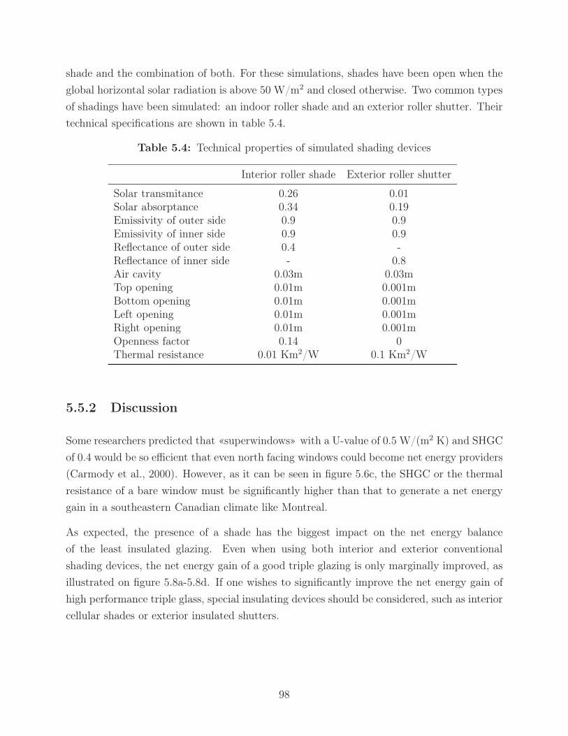
shade and the combination of both. For these simulations, shades have been open when the

global horizontal solar radiation is above 50 W/m2 and closed otherwise. Two common types

of shadings have been simulated: an indoor roller shade and an exterior roller shutter. Their

technical specifications are shown in table 5.4.

Table 5.4: Technical properties of simulated shading devices

Interior roller shade Exterior roller shutter

Solar transmitance 0.26 0.01Solar absorptance 0.34 0.19Emissivity of outer side 0.9 0.9Emissivity of inner side 0.9 0.9Reflectance of outer side 0.4 -Reflectance of inner side - 0.8Air cavity 0.03m 0.03mTop opening 0.01m 0.001mBottom opening 0.01m 0.001mLeft opening 0.01m 0.001mRight opening 0.01m 0.001mOpenness factor 0.14 0Thermal resistance 0.01 Km2/W 0.1 Km2/W

5.5.2 Discussion

Some researchers predicted that «superwindows» with a U-value of 0.5 W/(m2 K) and SHGC

of 0.4 would be so efficient that even north facing windows could become net energy providers

(Carmody et al., 2000). However, as it can be seen in figure 5.6c, the SHGC or the thermal

resistance of a bare window must be significantly higher than that to generate a net energy

gain in a southeastern Canadian climate like Montreal.

As expected, the presence of a shade has the biggest impact on the net energy balance

of the least insulated glazing. Even when using both interior and exterior conventional

shading devices, the net energy gain of a good triple glazing is only marginally improved, as

illustrated on figure 5.8a-5.8d. If one wishes to significantly improve the net energy gain of

high performance triple glass, special insulating devices should be considered, such as interior

cellular shades or exterior insulated shutters.

98

U (W/m2-K)

SHG

C

Energy gains per unit area (kWh/m2)

U, SHGC Bare glazing

U EffectiveU, SHGC Shade closed

DBclear

DBar-1low-e

DB-ARar-1low-e

DB-ARar-2low-eTriple

-300-250-200-150-100-500

50

100

150

200

250

300

350

400

450

500

0 0.5 1 1.5 2 2.5 30

0.1

0.2

0.3

0.4

0.5

0.6

0.7

0.8

0.9

(a) South

U (W/m2-K)

SHG

C

Energy gains per unit area (kWh/m2)

U, SHGC Bare glazing

U EffectiveU, SHGC Shade closed

DBclear

DBar-1low-e

DB-ARar-1low-e

DB-ARar-2low-eTriple

-300-250-200-150-100-500

50

100

150

200

250

300

0 0.5 1 1.5 2 2.5 30

0.1

0.2

0.3

0.4

0.5

0.6

0.7

0.8

0.9

(b) West

U (W/m2-K)

SHG

C

Energy gains per unit area (kWh/m2)

U, SHGC Bare glazing

U EffectiveU, SHGC Shade closed

DBclear

DBar-1low-e

DB-ARar-1low-e

DB-ARar-2low-eTriple

-300-250-200-150-100-500

50

100

0 0.5 1 1.5 2 2.5 30

0.1

0.2

0.3

0.4

0.5

0.6

0.7

0.8

0.9

(c) North

U (W/m2-K)

SHG

C

Energy gains per unit area (kWh/m2)

U, SHGC Bare glazing

U EffectiveU, SHGC Shade closed

DBclear

DBar-1low-e

DB-ARar-1low-e

DB-ARar-2low-eTriple

-300-250-200-150-100-500

50

100

150

200

250

0 0.5 1 1.5 2 2.5 30

0.1

0.2

0.3

0.4

0.5

0.6

0.7

0.8

0.9

(d) East

Figure 5.6: Net energy gain diagrams of a fenestration system with an exterior shade

99

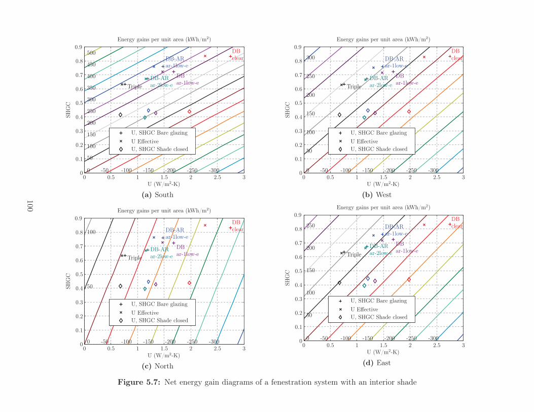
U (W/m2-K)

SHG

C

Energy gains per unit area (kWh/m2)

U, SHGC Bare glazing

U EffectiveU, SHGC Shade closed

DBclear

DBar-1low-e

DB-ARar-1low-e

DB-ARar-2low-eTriple

-300-250-200-150-100-500

50

100

150

200

250

300

350

400

450

500

0 0.5 1 1.5 2 2.5 30

0.1

0.2

0.3

0.4

0.5

0.6

0.7

0.8

0.9

(a) South

U (W/m2-K)

SHG

C

Energy gains per unit area (kWh/m2)

U, SHGC Bare glazing

U EffectiveU, SHGC Shade closed

DBclear

DBar-1low-e

DB-ARar-1low-e

DB-ARar-2low-eTriple

-300-250-200-150-100-500

50

100

150

200

250

300

0 0.5 1 1.5 2 2.5 30

0.1

0.2

0.3

0.4

0.5

0.6

0.7

0.8

0.9

(b) West

U (W/m2-K)

SHG

C

Energy gains per unit area (kWh/m2)

U, SHGC Bare glazing

U EffectiveU, SHGC Shade closed

DBclear

DBar-1low-e

DB-ARar-1low-e

DB-ARar-2low-eTriple

-300-250-200-150-100-500

50

100

0 0.5 1 1.5 2 2.5 30

0.1

0.2

0.3

0.4

0.5

0.6

0.7

0.8

0.9

(c) North

U (W/m2-K)

SHG

C

Energy gains per unit area (kWh/m2)

U, SHGC Bare glazing

U EffectiveU, SHGC Shade closed

DBclear

DBar-1low-e

DB-ARar-1low-e

DB-ARar-2low-eTriple

-300-250-200-150-100-500

50

100

150

200

250

0 0.5 1 1.5 2 2.5 30

0.1

0.2

0.3

0.4

0.5

0.6

0.7

0.8

0.9

(d) East

Figure 5.7: Net energy gain diagrams of a fenestration system with an interior shade

100

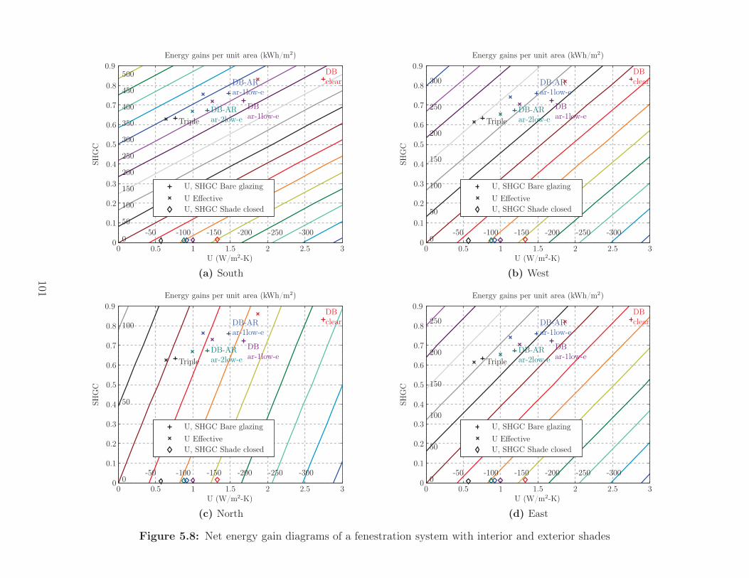
U (W/m2-K)

SHG

C

Energy gains per unit area (kWh/m2)

U, SHGC Bare glazing

U EffectiveU, SHGC Shade closed

DBclear

DBar-1low-e

DB-ARar-1low-e

DB-ARar-2low-eTriple

-300-250-200-150-100-500

50

100

150

200

250

300

350

400

450

500

0 0.5 1 1.5 2 2.5 30

0.1

0.2

0.3

0.4

0.5

0.6

0.7

0.8

0.9

(a) South

U (W/m2-K)

SHG

C

Energy gains per unit area (kWh/m2)

U, SHGC Bare glazing

U EffectiveU, SHGC Shade closed

DBclear

DBar-1low-e

DB-ARar-1low-e

DB-ARar-2low-eTriple

-300-250-200-150-100-500

50

100

150

200

250

300

0 0.5 1 1.5 2 2.5 30

0.1

0.2

0.3

0.4

0.5

0.6

0.7

0.8

0.9

(b) West

U (W/m2-K)

SHG

C

Energy gains per unit area (kWh/m2)

U, SHGC Bare glazing

U EffectiveU, SHGC Shade closed

DBclear

DBar-1low-e

DB-ARar-1low-e

DB-ARar-2low-eTriple

-300-250-200-150-100-500

50

100

0 0.5 1 1.5 2 2.5 30

0.1

0.2

0.3

0.4

0.5

0.6

0.7

0.8

0.9

(c) North

U (W/m2-K)

SHG

C

Energy gains per unit area (kWh/m2)

U, SHGC Bare glazing

U EffectiveU, SHGC Shade closed

DBclear

DBar-1low-e

DB-ARar-1low-e

DB-ARar-2low-eTriple

-300-250-200-150-100-500

50

100

150

200

250

0 0.5 1 1.5 2 2.5 30

0.1

0.2

0.3

0.4

0.5

0.6

0.7

0.8

0.9

(d) East

Figure 5.8: Net energy gain diagrams of a fenestration system with interior and exterior shades

101

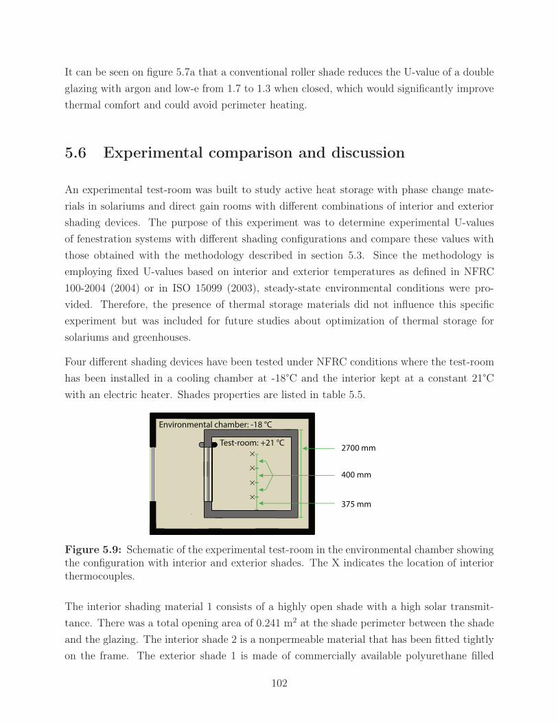
It can be seen on figure 5.7a that a conventional roller shade reduces the U-value of a double

glazing with argon and low-e from 1.7 to 1.3 when closed, which would significantly improve

thermal comfort and could avoid perimeter heating.

5.6 Experimental comparison and discussion

An experimental test-room was built to study active heat storage with phase change mate-

rials in solariums and direct gain rooms with different combinations of interior and exterior

shading devices. The purpose of this experiment was to determine experimental U-values

of fenestration systems with different shading configurations and compare these values with

those obtained with the methodology described in section 5.3. Since the methodology is

employing fixed U-values based on interior and exterior temperatures as defined in NFRC

100-2004 (2004) or in ISO 15099 (2003), steady-state environmental conditions were pro-

vided. Therefore, the presence of thermal storage materials did not influence this specific

experiment but was included for future studies about optimization of thermal storage for

solariums and greenhouses.

Four different shading devices have been tested under NFRC conditions where the test-room

has been installed in a cooling chamber at -18°C and the interior kept at a constant 21°C

with an electric heater. Shades properties are listed in table 5.5.

Environmental chamber: -18 °C

Test-room: +21 °C

400 mm

375 mm

2700 mm

Figure 5.9: Schematic of the experimental test-room in the environmental chamber showingthe configuration with interior and exterior shades. The X indicates the location of interiorthermocouples.

The interior shading material 1 consists of a highly open shade with a high solar transmit-

tance. There was a total opening area of 0.241 m2 at the shade perimeter between the shade

and the glazing. The interior shade 2 is a nonpermeable material that has been fitted tightly

on the frame. The exterior shade 1 is made of commercially available polyurethane filled

102

aluminum slats. The exterior shade 2 is a custom made panel made of vacuum insulated

panels (VIP) sandwiched between extruded polystyrene (XPS). Its thermal resistance has

been evaluated at R 2.19 Km2/W.

The test-room consists of a chamber 3 m long by 1.5 m wide and 2.7 m high simulating an

attached sunspace with a 2 m by 2 m double glazed window (glazing U-value=1.314 W/(m2K)

and SHGC=0.262). The glazing and framing area are 3.64 and 0.493 m2 respectively while

the U-value of the frame is 1.9 W/(m2K). The overall U-value of the window is 1.7 W/(m2K).

The air tightness of the test-room has been measured at different pressure differential levels

by performing blower door testing. The air infiltration at 50 Pa has been evaluated through

polynomial regression as 4.1 ACH and the infiltration rate under the tested conditions (-

18°C/+21°C) has been estimated as 0.2 ACH.

Four type T thermocouples (accuracy of 0.5°C) were located inside the test-room as shown

in figure 5.9 and four outside in the climatic chamber. An average temperature differ-

ence between the climatic chamber and the test-room of 37.7 °C was maintained during

the tests.

The electricity consumption of the heater was monitored for the unshaded test-room and

the five different shading configurations described in table 5.6. The U-value of the test room

attributed to the envelope (walls, ceiling and floor) has been evaluated as 0.35 W/(m2K). It

was calculated from the heater electricity consumption for the unshaded test-room and by

subtracting the losses due to the window and infiltration. The experimental U-value of the

fenestration system in a given configuration was determined from subtracting the heat losses

due to the envelope, window frame and infiltration to the heater electricity consumption.

The U-values of the different shade configurations obtained experimentally are compared in

table 5.6 with values that have been calculated following the methodology presented in this

paper.

Table 5.5: Technical properties of tested shading devicesaThe thermal resistance of the interior shades was too low to be measured; a value of0.01 W/(m2K) has been selected for simulations

Description Cavity width τs αs ε R OP Openingcm f/b Km2/W m2

Int shade 1 15.5 0.77 0.02 0.89 0.01a 0.52 0.241Int shade 2 9.4 0 0.37 0.49 0.01a 0 0Ext shade 1 5.4 0 0.28 0.79/0.76 0.080 0 0Ext shade 2 1.9 0 0.37 0.49 2.19 0 0

103

Table 5.6: Comparison of experimental and simulation results - U glazing = 1.314 W/(m2K)

U-value U-valueSimulated ExperimentalW/(m2K) W/(m2K)

Configuration

Window/Int shade 1 1.09 1.18Window/Int shade 2 0.97 1.04Ext shade 1/Window 0.99 0.99Ext shade 2/Window 0.31 0.45Ext shade 1/Window/Int shade 1 0.86 0.96

As can be seen from table 5.6, simulated and experimental U-values are relatively close to

each other, with simulation results having a general tendency to be lower than experimental

values.

The interior shade 1 has a high openness factor of 0.52 while the interior shade 2 is totally

impervious to air. It should also be noted that the interior shade 2 was installed in an airtight

fashion while there were large openings around the interior shade 1. Even with such a large

openness factor, openings around the shades and a relatively wide cavity, measurements are

showing that the interior shade 1 improves the glazing U-value by 10%. The simulated U-

value of the exterior shade 2 is significantly lower than measured. This is probably mainly

due to the uncertainty related to the determination of the overall thermal resistance of the

shade, which is made of a combination of VIP and EXP, arranged non uniformly in order to

cover completely the glazing.

Experimental results might be indicating that the sensitivity to the openness factor and

openings area is more important in reality than what is calculated with the ISO 15099

model, but a more thorough experimental validation would be needed to confirm this. It

should be noted that there are no restrictions concerning the range of openness factor in ISO

15099.

The most significant uncertainty in the modelling of the heat transfer through fenestration

systems probably pertains to the calculation of the convective heat transfer coefficient in

the cavity between the glazing and shading layers. Although the algorithm developed in

ISO 15099 has been implemented in many important building energy simulation software

(EnergyPlus, WINDOW, WIS) and used to conduct comprehensive simulations of various

window attachments (Curcija et al., 2013), there is a lack of experimental validation in the

published literature to date. A study conducted with diffuse interior and exterior shading

104

screens revealed discrepancies in the ability of various building energy simulation programs

to model the heat transfer in the cavity between the shading and glazing layers (Loutzen-

hiser et al., 2007). The development of a simple yet accurate model or correlation for the

determination of the convective cavity heat transfer coefficient is an important area for future

research.

The ASHWAT model (Wright et al., 2009) developed an approximate model that allows the

calculation of the impact of the cavity width on the convective coefficients in the vicinity of a

shade, based on the two limiting cases (where the shade is far away from a window or where

the spacing approaches zero). It is acknowledged that this model is only an approximation

and that future research should be conducted regarding the convective heat transfer coefficient

in the glazing/shading cavity. The ASHWAT model also developed useful correlations for

the determination of solar optical properties of venetian blinds, drapes, screens and roller

shades (Kotey et al., 2009a,b,d,c). It should be noted that for the latter, the openness factor

must not be higher than 0.2.

Although there has been significant advancement in the last decades in the evaluation of

the thermal performance of shading devices, challenges remain due to the complexity of

the heat transfer in complex fenestration systems (Laoudi, 2009). Should simpler validated

physical models or more accurate empirical correlations be developed in the future that

better describe the heat transfer through fenestration systems, they could easily replace the

equations suggested in this methodology.

5.7 Conclusion

This paper presented a methodology to help in the selection of fenestration systems for

buildings in heating dominated climates. The method has the capability to simulate a one or

two layer shading system with one exterior and/or one interior planar shade. This method

generates 2D schematics indicating lines of constant net energy gain per unit area as a

function of the SHCG and U-value on which different fenestration components are situated.

Such graphics are useful in early design stage to compare different design options on a relative

basis for a specific orientation and climate.

The essence of the method is based on the computation of the useful solar gains through

fenestration and associated heat losses when the exterior temperature is below the balance

temperature. This methodology is intended to be used for the design of buildings aiming at

105

a high solar utilization like solar houses, solariums/greenhouses and buildings adopting the

solar optimized fenestration systems design concept. It has the capability to evaluate the

performance of either glazings or complete windows in combination with a one or two layer

shading system. Once implemented, this methodology can be readily used for new or retrofit

projects in different locations.

This methodology can be used independently or as a preliminary design tool to help identi-

fying the best performing combinations of windows and shades as a function of orientation

before running whole building energy simulations.

This paper presented diagrams for glazings equipped with an interior roller shade, an exterior

roller shutter and a combination of both for the four cardinal orientations for the city of Mon-

treal, Canada. A comparison of simulated and experimental U-values of four shading devices

revealed results relatively close to each other, but additional research on the convective heat

transfer coefficient in the cavity between the shading and glazing layers is needed.

106

Chapter 6

Development of a new control strategy

for improving the operation of multiple

shades in a solarium

Based on a published paper:

Bastien, D., Dermardiros, V. and Athienitis, A. 2015b. Development of a new control strat-

egy for improving the operation of multiple shades in a solarium. Solar Energy, 122, 277-

292.

6.1 Chapter abstract

This chapter presents a new control strategy for improving the performance of one interior

and/or exterior planar shade(s). The control strategy is based on performing an energy

balance on the fenestration system and calculating the total heat flow (i.e. solar gains +

overall heat losses). The heat flow can be maximized or minimized depending on the needs

of the space. A solarium model was developed in order to assess the performance of the

proposed shading strategy. The solarium model can simulate passive and active thermal

storage using sensible and phase change materials. A prototype solarium with motorized

interior and exterior shadings has been instrumented and subjected to controlled conditions.

The numerical simulations are in good agreement with experimental results.

107

The simulation model has then been used to perform annual simulations of an attached

solarium for the location of Montreal, Canada. The year was divided in a heating mode and

a mixed mode. During the heating mode (i.e. October through April), heating is provided to

keep a minimum temperature of 10°C and surplus heat is considered when the temperature

reaches 28°C. By using the proposed algorithm for the control of one interior and/or exterior

shade(s) in the heating mode, heating requirements of the simulated solarium have been

reduced by 3-9% and an additional 9-14% of surplus heat have been collected when compared

to a control based on near optimum global horizontal solar radiation levels. During the mixed

mode, thermal comfort can be improved significantly (+1822 hours) when the interior shade

is controlled with the proposed algorithm.

6.2 Introduction

Shading devices are commonly used in various building types such as residential buildings,

offices buildings, solariums and greenhouses. They are mainly used for reducing solar gains

and heat losses, controlling glare and improving daylight availability.

In solariums and greenhouses, the former two objectives typically prevail. Attached solar-

iums are one of the most popular passive solar systems (Mihalakakou and Ferrante, 2000).

Integrated to either new or existing houses, they are generally built to gain additional floor

space with abundant daylight. In addition, solariums also have the potential to provide ad-

equate conditions for growing plants and vegetables, as well as collecting solar heat. With

their large glazing area, the use of shades and their control may affect significantly the energy

requirements and thermal comfort in a solarium.

Generally in greenhouses, a shade whose main purpose is to reject near infrared radiation for

temperature control is called a solar screen, while a shade whose main purpose is to reduce

heat losses is called a thermal screen. Many studies reported significant energy savings due

to the implementation of thermal screens in greenhouses. For different types of greenhouses

and screens, the use of a thermal screen from sunset to sunrise has been shown to reduce

the energy used by 27% to 43% (Meyer, 1981), 21% to 33% (Bailey, 1988) and 16% (Diele-

man and Kempkes, 2006) for greenhouses located in Germany, England and Netherlands,

respectively.

The addition of shades to the windows of residential buildings has been shown to be useful

for reducing heat losses. Simulations carried out by Selkowitz and Bazjanac (1979) have

shown that the net annual heating requirements of a house can be reduced by 18% when R10

108

shutters are closed twelve hours at night for equally distributed single pane windows (with

a window to floor ratio of 15% in Minneapolis). When used with clear double glass, the net

annual heating requirements can be reduced by 9%.

Simulations have shown that the use of roller shades in office buildings with continuously

dimmable lights could lower the source energy consumption up to 7% while improving visual

comfort (Tzempelikos and Shen, 2013). The use of more sophisticated devices like an actively

controlled venetian blind was estimated to reduce the energy for heating, cooling and artificial

lighting by up to 22% (Nielsen et al., 2011).

6.2.1 Existing shading control strategies

Many studies have been conducted about the operation of different types of movable shading

devices and their associated energy performance. Studies on office buildings generally focus

on reducing heating and cooling loads, artificial lighting and glare while providing adequate

workplane illuminance.

Various shading control strategies for offices buildings have been investigated such as those

based on

• Time clock operation (Yao, 2014).

• Incident solar irradiance (van Moeseke et al., 2007).

• Incident total or beam radiation (Lee and Selkowitz, 2006; Wienold, 2007; Tzempelikos

and Shen, 2013).

• Incident or transmitted illuminance (Galasiu et al., 2004; Tzempelikos and Shen, 2013).

• Preventing direct sunlight from falling on the workplane (Tzempelikos and Shen, 2013).

• The illuminance level at the workplane (Wienold, 2007).

• Minimizing the total heat gains when in cooling mode (with additional criteria) (Tzem-

pelikos and Shen, 2013).

• Fixed blind tilt angle (for venetian blinds) (Carbonari et al., 2001; Galasiu et al., 2004;

Huang et al., 2014).

• The cut-off angle to block beam radiation (for venetian blinds) (Wienold, 2007; Nielsen

et al., 2011; Shen et al., 2014).

• Internal temperature (van Moeseke et al., 2007).

• A combination of solar irradiance and internal temperature (van Moeseke et al., 2007).

• Others (Carbonari et al., 2001; Lee and Selkowitz, 2006; Wienold, 2007; Shen et al.,

2014).

109

Tzempelikos and Shen (2013) carried out comprehensive thermal and lighting simulations of

four different shading control strategies for operating roller shades in office buildings. They

mention that the transmitted illuminance is a more appropriate metric than an incident solar

radiation set point for providing visual comfort with shade control, especially for spectrally

selective windows with low solar gains. They note that the glazing type and shading prop-

erties have a significant impact on the performance of different shading controls, while their

results indicate that the best shading control type for a specific climate and building remains

essentially the same regardless of glazing type and shading properties.

Thermal conditions and requirements in solariums and greenhouses differ largely from those

prevailing in office buildings; therefore appropriate control strategies for operating shading

devices may also be different.

Control strategies for operating solar and thermal screens in greenhouses can be based on

several approaches such as:

• Time clock operation (Seginer and Albright, 1980).

• A fixed value of solar radiation (Marsh et al., 1984; Dieleman and Kempkes, 2006).

• A linear correlation between solar radiation and outside temperature (Marsh et al.,

1984; Dieleman and Kempkes, 2006).

• A combination of internal temperature and incident solar radiation (Lorenzo et al.,

2003).

• An economic criteria based on energy saved versus crop loss (Aaslyng et al., 2003).

It was found that energy savings can be increased by 6% when the screen is controlled based

on radiation level compared to time clock operation (Seginer and Albright, 1980). Marsh

et al. (1984) measured an energy saving of 3.3% when the opening of thermal screens was

based on an inside light level of 30 W/m2 compared to time clock operation. This study also

concluded that using a more advanced control strategy based on a light level that is a linear

function of the outside temperature may not be justified because no additional savings were

observed compared to a fixed light level control.

Simulations carried out by Dieleman and Kempkes (2006) have shown that by opening a

thermal screen based on increasing the outside radiation level from 1 W/m2 to 25, 50 and

150 W/m2, an additional energy saving of 2%, 3% and 4% respectively can be achieved. The

same study found that screen operation based on correlations of outside temperature and

radiation can achieve a similar energy reduction of up to 4%.

110

Aaslyng et al. (2003) developed an indoor environment control system for greenhouses based

on a combination of control methods. Thermal screens were controlled to maximize profit,

which was calculated as a trade-off between the energy saved with screens on versus the

production loss caused by decreased irradiance. The operating temperature range was con-

siderably wider than usual; the temperature was lower on cloudy days where growth is re-

duced and higher on sunny days to increase production. Field tests showed significant energy

savings with only small changes in plant production.

6.2.2 Benefits of thermal storage and its influence on the energy

consumption of various building types

Integrating thermal mass in buildings can provide significant benefits for various building

types and climates. An exterior wall with insulation on the outside and interior mass sub-

jected to daily solar gains exhibits reduced temperature swings and a delay between the

peak solar gains and the resulting peak of the room temperature (Athienitis and O’Brien,

2015).

Through simulations, Kosny et al. (2001) have evaluated that by replacing lightweight wood

frame construction with massive constructions of the same R-value, annual energy savings of

up to 8% can be achieved for residential buildings in cold climates and up to 18% in warm

climates. To achieve these results, the thermal mass must be in good contact with the interior

of the building. Wall R-values between 0.9 to 4.4 m2 K/W (R5 to R25) have been simulated.

It is interesting to note that energy savings increase with R-values in both climates; thus

higher energy savings might be obtained with R-values above 4.4 m2 K/W.

Simulations conducted by Braun (1990) on office buildings with varying properties in different

climates showed possible energy cost savings between 10-50% and peak power reduction

between 10-35% when the building structure is used for thermal storage. The study of 12

low-energy office buildings in Germany revealed that good thermal comfort in summer is

achievable without mechanical cooling, providing that buildings are designed for low solar

and internal gains, with an adequate thermal storage capacity and a sufficient heat sink

(Pfafferott et al., 2007).

Thermal mass is extensively used in solariums and greenhouses. Because these spaces are

subjected to greater solar gains and temperature fluctuations than residential and office

buildings, greater reductions in energy requirements may be obtained by including thermal

storage materials. Many different thermal storage systems have been investigated; a review

111

of these is presented in Sethi and Sharma (2008). In this review, earth-to-air heat exchange

systems are reported to reduce heating requirements between 28 to 62% and north walls

storage systems between 35 to 82%. A review of greenhouses using phase change materials

(PCM) for energy storage applications has been conducted by Kurklu (1998). All studies

under review suggested that PCM could be efficiently used for energy storage in greenhouses

with reported energy savings from 30% to 80%.

From this brief review, it can be seen that thermal mass can be useful in virtually all buildings

types and climates, although the magnitude of the energy savings is strongly affected by the

building type and operation, thermal storage material and configuration and climate.

As described in the next section, this paper presents a control strategy for operating shades

based on maximizing the total heat flow through fenestration systems. Maximizing the net

heat flow through fenestration systems is an interesting concept whose benefits are fully

realized only when solar gains are useful. The inclusion of thermal storage materials in

buildings is an important element for maximizing the energy gains obtained by using the

control strategy proposed here.

6.2.3 Objectives and overview

Although many studies have been conducted regarding efficient shading control, the authors

are not aware of any published method for operating shades based on an energy balance on the

fenestration system. The aim of this study is to develop a new control strategy for improving

the performance of shades that is based on performing an energy balance on the fenestration

system. In order to do so, detailed mathematical and numerical models of a solarium are

developed. The best position of a shade is either totally open or totally closed; the position

selected is the one that maximizes or minimizes the net heat flow of the glazing-shade system

(referred to as fenestration system throughout this study). This control strategy can be used

for the control of an interior shade, an exterior shade or a combination of both.

Section 6.3 presents the mathematical and numerical models of a solarium used for imple-

menting the shading control strategy. Section 6.4 presents a comparison of the simulation

model with experimental data obtained by instrumenting a solarium test-room placed in

an environmental chamber under illumination provided by a solar simulator. The proposed

shading control algorithm is presented in Section 6.5. Details about the applications of this

methodology, its limitations and some recommendations are provided in section 6.6.

112

6.3 Solarium model

The solarium model can be fully glazed or be made of a combination of glazed surfaces and

opaque walls. The glazed surfaces may be covered by an exterior and/or an interior shade.

These shades can be used for improving the thermal resistance and thermal comfort in winter

and for reflecting solar heat in summer.

The developed model consists of a detailed transient finite difference thermal network model

that includes modelling of one or two thermal storages. One thermal storage is located on the

floor, while the other one is located on one wall, ideally the north wall. Either conventional

sensible heat storage materials or phase change materials can be modelled. Thermal storages

can be made up of one layer passively charged and discharged or two layers separated by a

channel with active air circulation.

The inputs of the model are read from a Canadian Weather year for Energy Calculation

(CWEC) file. Any hourly weather data publicly available on the U.S. Department of Energy

(U.S. Department of Energy, 2015) website can be downloaded and used as input. The

required inputs consist of the global horizontal radiation, direct normal radiation, diffuse

horizontal radiation, wind speed, exterior temperature and relative humidity. Hourly values

are read and interpolated to fit the chosen time step.

6.3.1 Mathematical model

6.3.1.1 Solar radiation incident on sloped surfaces

Conventional equations based on geometrical relationships and the Perez model (Perez et al.,

1990) are used to evaluate the diffuse and beam solar radiation incident on a surface. They

are presented in section 4.1.1.

6.3.1.2 Solar radiation distribution on interior surfaces

Since it was found that only 30%-90% of radiation transmitted through the glazing is retained

in a highly glazed space such as a solarium or a greenhouse (Wall, 1995), the solar radiation

distribution on interior surfaces is modelled here with a detailed method combining ray

tracing and radiosity techniques which is presented in section 4.1.2.

113

6.3.1.3 Convective heat transfer

Correlations derived by Khalifa and Marshall (1990) are used for the calculation of convective

heat transfer coefficients of interior surfaces. They are presented in section 4.2, along with

the exterior convective coefficient due to wind.

Convective coefficients for air spaces between window panes and between windows and shad-

ing devices are calculated following the procedure outlined in ISO 15099 (2003) for thermally

driven ventilation, presented in section 4.2.

In the presence of an active thermal storage, the storage mass is divided into two layers

separated by a ventilated air channel. The heat exchange in the ventilated air gap is modelled

using control volumes. The air and surfaces temperature is assumed constant in each control

volume. Typically three or four control volumes are sufficient to adequately capture the heat

transfer. The convective coefficient in the air channel is calculated with

hc,ch =Nu k

Dh(6.1)

where the calculation of the Nusselt number is based on the correlations developed by Can-

danedo et al. (2011) for the front and back surfaces separately.

6.3.1.4 Radiative heat transfer

Long wave radiation exchanges between interior surfaces are modeled using the Gebhart

method (Gebhart, 1959; Mottard and Fissore, 2007), which is detailed in section 4.3.

Longwave radiation exchange between an exterior surface and the ground, sky and air is

given by

qLWR,o = qgnd + qsky + qo (6.2)

where equations for calculating qgnd, qsky and qo are presented in section 4.3.

Radiative heat transfer between panes of glass and in glazing/shade cavities are calculated

based on the fundamental equation for two infinite parallel plates, also presented in section

4.3. The radiative and convective coefficients of glazing and shading systems are calculated

individually at every time step to take into account variations due to temperature.

114

6.3.1.5 Thermal Storage

The model offers the possibility to include two thermal storages: one located on the floor

and one located on one wall. The wall thermal storage may be made of only one layer or

two layers with active air circulation in between. The thermal storages may be composed of

sensible or phase change materials (PCM). In particular, one possible design consists of PCM

panels located on the north wall separated by an air channel with active recirculation. Active

ventilation enhances thermal coupling between the indoor air and the thermal storage. In

addition, it enables a more effective storage of excess heat and its release when needed.

Latent heat storage is accumulating or releasing heat during the phase change occurring at

the phase transition temperature. The latent heat for a given mass of substance is given

by

Q = mλ (6.3)

Heat transfer in PCM is usually modeled using finite difference or finite elements methods.

The two most common modeling methods are the enthalpy method and the heat capacity

method (Lamberg et al., 2004). The heat capacity method is intuitive and easy to program

since the heat capacity accounts for both sensible and latent heat transfer. It allows the

modeling of non-isothermal phase change, which is frequently observed for non-pure mate-

rials. The heat capacity can be estimated from results obtained by a differential scanning

calorimeter (DSC) (Al-Saadi and Zhai, 2013). If not available, an effective heat capacity can

be estimated with

ceff =λ

T2 − T1

+ cp (6.4)

where T1 is the temperature where melting (or solidification) begins and T2 is the temperature

at which the material is completely melted (or solidified). Hysteresis can be accounted for

by calculating the effective heat capacity separately for melting and freezing or by using the

heat capacity curves obtained by DSC for freezing and melting, if available.

Due to its ease of implementation and its suitability for modelling materials with gradual

phase changes, the heat capacity method was chosen for this study where the latent heat

transfer is simulated using empirical results obtained by DSC to approximate the heat ca-

pacity.

115

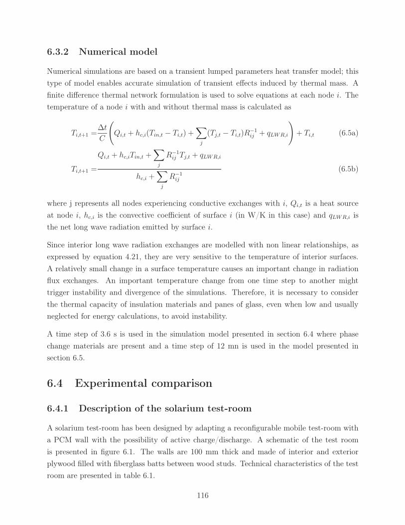
6.3.2 Numerical model

Numerical simulations are based on a transient lumped parameters heat transfer model; this

type of model enables accurate simulation of transient effects induced by thermal mass. A

finite difference thermal network formulation is used to solve equations at each node i. The

temperature of a node i with and without thermal mass is calculated as

Ti,t+1 =Δt

C

(Qi,t + hc,i(Tin,t − Ti,t) +

∑j

(Tj,t − Ti,t)R−1ij + qLWR,i

)+ Ti,t (6.5a)

Ti,t+1 =

Qi,t + hc,iTin,t +∑

j

R−1ij Tj,t + qLWR,i

hc,i +∑

j

R−1ij

(6.5b)

where j represents all nodes experiencing conductive exchanges with i, Qi,t is a heat source

at node i, hc,i is the convective coefficient of surface i (in W/K in this case) and qLWR,i is

the net long wave radiation emitted by surface i.

Since interior long wave radiation exchanges are modelled with non linear relationships, as

expressed by equation 4.21, they are very sensitive to the temperature of interior surfaces.

A relatively small change in a surface temperature causes an important change in radiation

flux exchanges. An important temperature change from one time step to another might

trigger instability and divergence of the simulations. Therefore, it is necessary to consider

the thermal capacity of insulation materials and panes of glass, even when low and usually

neglected for energy calculations, to avoid instability.

A time step of 3.6 s is used in the simulation model presented in section 6.4 where phase

change materials are present and a time step of 12 mn is used in the model presented in

section 6.5.

6.4 Experimental comparison

6.4.1 Description of the solarium test-room

A solarium test-room has been designed by adapting a reconfigurable mobile test-room with

a PCM wall with the possibility of active charge/discharge. A schematic of the test room

is presented in figure 6.1. The walls are 100 mm thick and made of interior and exterior

plywood filled with fiberglass batts between wood studs. Technical characteristics of the test

room are presented in table 6.1.

116

�����

�����

����

�����

�����

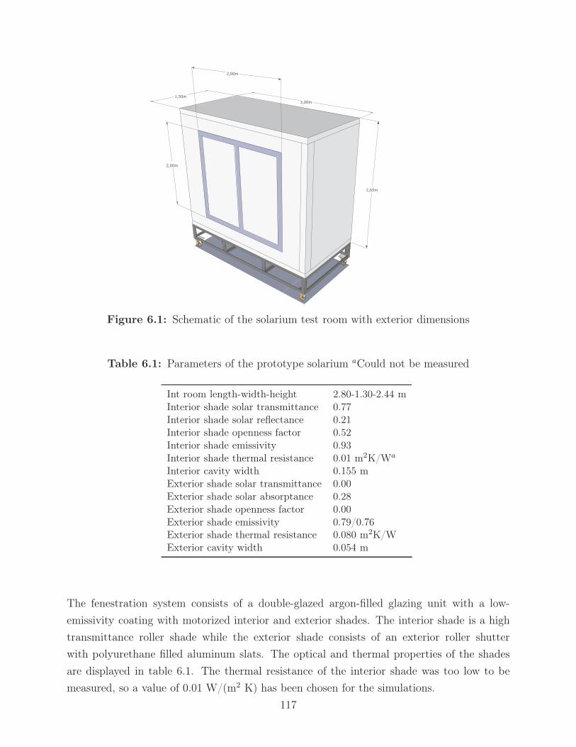
Figure 6.1: Schematic of the solarium test room with exterior dimensions

Table 6.1: Parameters of the prototype solarium aCould not be measured

Int room length-width-height 2.80-1.30-2.44 mInterior shade solar transmittance 0.77Interior shade solar reflectance 0.21Interior shade openness factor 0.52Interior shade emissivity 0.93Interior shade thermal resistance 0.01 m2K/Wa

Interior cavity width 0.155 mExterior shade solar transmittance 0.00Exterior shade solar absorptance 0.28Exterior shade openness factor 0.00Exterior shade emissivity 0.79/0.76Exterior shade thermal resistance 0.080 m2K/WExterior cavity width 0.054 m

The fenestration system consists of a double-glazed argon-filled glazing unit with a low-

emissivity coating with motorized interior and exterior shades. The interior shade is a high

transmittance roller shade while the exterior shade consists of an exterior roller shutter

with polyurethane filled aluminum slats. The optical and thermal properties of the shades

are displayed in table 6.1. The thermal resistance of the interior shade was too low to be

measured, so a value of 0.01 W/(m2 K) has been chosen for the simulations.

117

The U-value and SHGC of the insulated glazing unit have been simulated with Window 6.3

(LBNL, 2014) under NFRC conditions as 1.314 W/(m2 K) and 0.262. The U-value of the

frame has been evaluated by an independent laboratory as 1.9 W/(m2 K). The radiation

emitted by the solar simulator transmitted through the window has been calculated from

measurements obtained with a pyranometer mounted on a mobile arm as 0.34. Long wave

radiation exchanges between the window and the hot lamps from the solar simulator had to

be considered.

The air tightness has been measured at different pressure differential levels. The overall U-

value of the test room with retracted shades and no PCM has been experimentally measured

under steady-state conditions as 0.56 W/(m2 K). After calibrating the model, the infiltration

rate under normal conditions has been estimated as 0.25 ACH and the overall U-value of the

test room for the walls, floor and ceiling (no fenestration nor infiltration) was evaluated at

0.4 W/(m2 K).

Commercial PCM wallboards made of a mixture of an ethylene-based polymer and paraffin

60%wt were installed on the back wall. Three layers of PCM were installed on the front side

and two layers on the back side with a 30 mm channel for active air circulation in between.

This air channel was continuously ventilated with an air velocity of 1.5 m/s.

Four panels were necessary to fully cover the back wall and were treated as one continu-

ous layer with uniform temperature. With five layers of PCM, the 20 installed panels are

equivalent to a total latent storage capacity of about 7540 kJ (or 2.1 kWh). There were

two additional layers of polystyrene insulation behind the PCM layers. Figure 6.2 shows the

geometry of this active PCM wall thermal storage.

According to manufacturer’s data, the melting point of this PCM is 21.7°C with a latent heat

of fusion of 70 kJ/kg. For a temperature difference from 0 to 30 °C, the total heat stored

per panel would be about 755 kJ or 140 kJ/kg. The properties of these PCM boards have

been analyzed in other studies and their properties are summarized in table 6.2 for various

sources. There are some relatively important discrepancies.

In the present study, the average mass of one panel was determined as 6.074 kg, yielding a

density of 973 kg/m3. The specific heat capacity method was implemented where specific

heat capacities were evaluated from DSC curves for melting and freezing reported in Kuznik

and Virgone (2009). The conductivity of the PCM was evaluated at a given temperature

using the curves published in Kuznik et al. (2008).

118

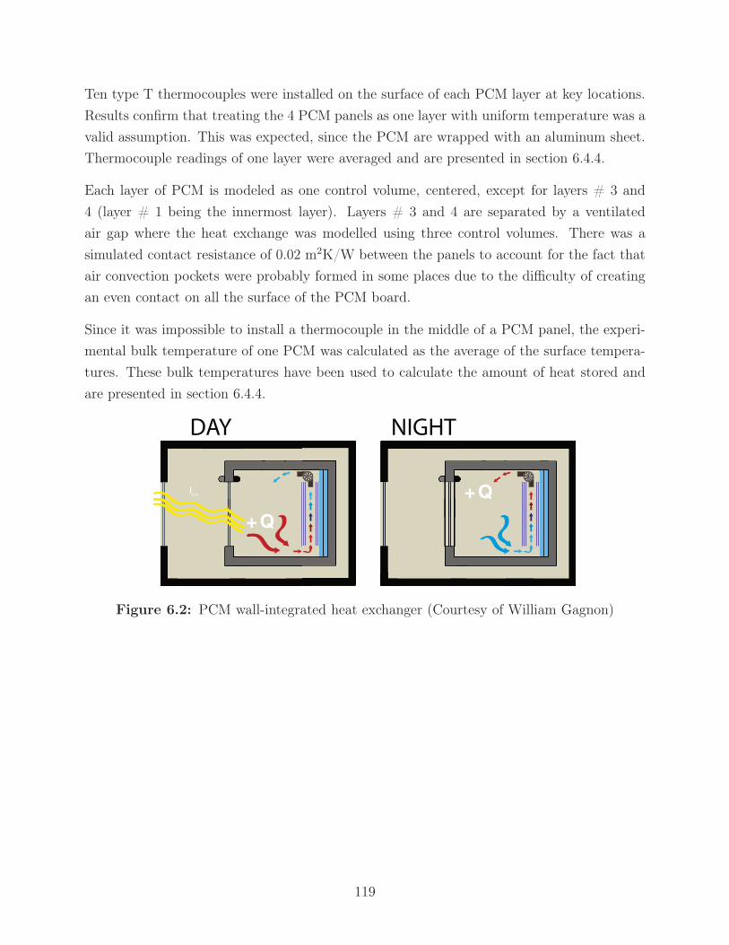
Ten type T thermocouples were installed on the surface of each PCM layer at key locations.

Results confirm that treating the 4 PCM panels as one layer with uniform temperature was a

valid assumption. This was expected, since the PCM are wrapped with an aluminum sheet.

Thermocouple readings of one layer were averaged and are presented in section 6.4.4.

Each layer of PCM is modeled as one control volume, centered, except for layers # 3 and

4 (layer # 1 being the innermost layer). Layers # 3 and 4 are separated by a ventilated

air gap where the heat exchange was modelled using three control volumes. There was a

simulated contact resistance of 0.02 m2K/W between the panels to account for the fact that

air convection pockets were probably formed in some places due to the difficulty of creating

an even contact on all the surface of the PCM board.

Since it was impossible to install a thermocouple in the middle of a PCM panel, the experi-

mental bulk temperature of one PCM was calculated as the average of the surface tempera-

tures. These bulk temperatures have been used to calculate the amount of heat stored and

are presented in section 6.4.4.

ISUN

DAY NIGHT

+Q

+Q

Figure 6.2: PCM wall-integrated heat exchanger (Courtesy of William Gagnon)

119

Table 6.2: Technical specifications of PCM panels from various sources

Manufacturer Kuznik et al. (2008) Kuznik and Virgone (2009) Tabares-velasco et al. (2012)(HR 1 °C/mn) (HR 2 °C/mn) (HR 0.05 °C/mn) (HR 0.05 °C/mn)

Mass 5.391 kgDimensions 1000 x 1198 mmThickness 5.2 mm 5.3 mmDensity 855.5 kg/m3 1019 kg/m3 ≈ 900 kg/m3 855 kg/m3

T melting 21.7°C ≈ 22 °CT melting p 22.2 °C 22.3 °C 23.3 °CT freezing p 17.8 °C

Latent heat, melting >70 000 J/kg 72 400 J/kgLatent heat, freezing 71 000 J/kg

Cp - sensible 2333 J/(kg°C) 2500 J/(kg°C)Cp - melting p 15 200 J/(kg °C) 13 400 J/(kg °C) 13 810 J/(kg °C)Cp - freezing p 12 900 J/(kg °C)Cp - solid 2400 J/(kg°C)

Conductivity - solid 0.18 W/(mK) 0.22 W/(mK) 0.18 W/(mK)a 0.18Conductivity - liquid 0.14 W/(mK) 0.18 W/(mK) 0.22 W/(mK) a 0.14

aNot consistent with the author’s previous study conductivity curve, values were probably inverted inadvertently

120

6.4.2 Experimental facility

The experimental work took place in the Solar Simulator - Environmental Chamber at Con-

cordia University, which features two solar simulators and a climatic chamber. The environ-

mental chamber can provide temperatures varying between -40°C and +50°C and a relative

humidity between 20% and 95%. This unique facility enables accurate and repeatable testing

of solar systems and advanced building envelopes under controlled conditions.

The test solarium was placed inside the climatic chamber and subjected to radiation emit-

ted by a full-scale solar simulator. Pictures of the experimental facility are shown in fig-

ure 6.3.

(a) Solar simulator and environmental chamber (b) Test solarium under illumination

Figure 6.3: Experimental facility

6.4.3 Testing conditions

The cyclic solar radiation profile and constant outdoor temperature selected for the exper-

iment are illustrated in figure 6.4. The average temperature surrounding the test solarium

throughout the experiment was measured as 5.7°C. The solarium was illuminated three hours

per day. The average radiation incoming on the window at the first and last sunny hour was

measured with a pyranometer as 502 W/m2 while it reached 1033 W/m2 for the peak hour.

121

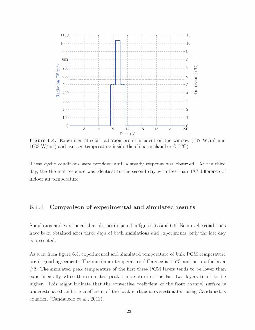
Rad

iati

on(W

/m2)

Tem

per

atur

e(°

C)

Time (h)3 6 9 12 15 18 21 24

0

1

2

3

4

5

6

7

8

9

10

11

0

100

200

300

400

500

600

700

800

900

1000

1100

Figure 6.4: Experimental solar radiation profile incident on the window (502 W/m2 and1033 W/m2) and average temperature inside the climatic chamber (5.7°C).

These cyclic conditions were provided until a steady response was observed. At the third

day, the thermal response was identical to the second day with less than 1°C difference of

indoor air temperature.

6.4.4 Comparison of experimental and simulated results

Simulation and experimental results are depicted in figures 6.5 and 6.6. Near cyclic conditions

have been obtained after three days of both simulations and experiments; only the last day

is presented.

As seen from figure 6.5, experimental and simulated temperature of bulk PCM temperature

are in good agreement. The maximum temperature difference is 1.5°C and occurs for layer

#2. The simulated peak temperature of the first three PCM layers tends to be lower than

experimentally while the simulated peak temperature of the last two layers tends to be

higher. This might indicate that the convective coefficient of the front channel surface is

underestimated and the coefficient of the back surface is overestimated using Candanedo’s

equation (Candanedo et al., 2011).

122

Time(hr)

Tem

per

atur

e(°

C)

T1T2T3T4T5

4 8 12 16 20 2414

16

18

20

22

24

26

28

30

32

34

Figure 6.5: Experimental (solid) and simulated (dashed) bulk temperature of PCMs layers

Time(hr)

Tem

per

atur

e(°

C)

Ti

Tmean radiant

4 8 12 16 20 2414

16

18

20

22

24

26

28

30

32

34

Figure 6.6: Experimental (solid) and simulated (dashed) indoor air temperature and meanradiant temperature

123

As depicted in figure 6.6, simulations of indoor and mean radiant air temperature are in good

agreement with experimental results. The maximum absolute temperature difference is 1.0

°C for the air temperature and is 0.8 °C for the mean radiant temperature. The discontinuity

of the specific heat occurring during a partial phase transition was not corrected. Using a

model for transitioning inside the phase change zone such as the one suggested in Bony and

Citherlet (2007) could improve the model.

The heat stored and released by each PCM layer has been calculated from the experimental

bulk temperature and is presented in table 6.3. The associated uncertainty is presented in

Appendix B. The heat stored per kilogram in the given experimental conditions is signifi-

cantly higher than what is stated by the manufacturer. This is explained by the difficulty

in evaluating the sensible specific heat of a PCM. While the reported sensible specific heat

of this PCM lies between 2333 and 2500 J/(kg°C) as seen from table 6.2, it can be seen in

Kuznik and Virgone (2009) that the specific heat at 5 and 30°C is respectively 3724 and

2640 J/(kg°C) for melting and 4027 and 2557 J/(kg°C) for freezing.

Table 6.3: Heat stored and released in PCMs for a diurnal cycle

Heat stored Heat released Total temperaturePer layer Per kg Per layer Per kg variation(kJ) (kJ/kg) (kJ) (kJ/kg) (°C)

Layer 1 8 260 336 7 328 298 34.1Layer 2 7 409 302 6 507 265 25.6Layer 3 6 971 284 6 260 255 22.2Layer 4 4 301 175 4 974 202 13.5Layer 5 3 453 141 4 362 178 11.6Total 30 393 247 29 431 240

6.5 Shading control strategy

6.5.1 Design of the simulated solarium

A south facing attached solarium has been modelled as described in section 6.3. The solarium

is 10 meters long and 2.4 meters wide with a south roof angle of 35°. It is attached to a

house with a thermally massive common wall made of two layers of bricks of a thickness of

200 mm each separated by a 40 mm air channel. The back side of the second layer of bricks

is insulated with RSI 10.6 (R60). The temperature in the house is maintained at a constant

20°C. There is also a passive thermal storage that consists of a 200 mm concrete floor. The

infiltration rate is set to 0.1 air change per hour throughout the year.

124

�����

����

���� �����

Figure 6.7: Simulated attached solarium

Simulations were conducted with clear double glass. The solarium is equipped with an interior

roller blind and an exterior roller shutter, both motorized. Shades were assumed to be parallel

to the glazing and to cover both glazing and framing members. For the energy control scheme,

shades with different orientations can be controlled independently. The cavity between the

exterior shade and the window is 50 mm while the cavity between the indoor shade and the

window is 30 mm. The opaque roller shutter has a thermal resistance of 0.1 m2K/W and

an emissivity of 0.8. The interior roller blind has a solar transmittance of 0.19 and a solar

reflectance of 0.71. An interior shade with such a high solar reflectance is useful both in the

heating season by reflecting the solar gains from other glazed surfaces inside the space and

in the warmer season by reflecting direct solar radiation outside the space.

6.5.2 Shading control algorithm

This control algorithm is based on performing an energy balance on the fenestration system.

In this study, the total heat flow through a fenestration system is calculated as:

• Solar radiation transmitted through the fenestration system and absorbed by interior

surfaces

• + Heat flow through the fenestration system from outdoor to the zone

To evaluate the effect of moving one shade on the solar gains from other glazed surfaces, it

is necessary to consider the solar radiation gained or lost from other fenestration systems by

moving the position of that shade. Therefore, when calculating the total heat flow through

a fenestration system in a different state, the following term must be added:

• + Solar radiation gained or lost from other fenestration systems by moving the position

of the shade125

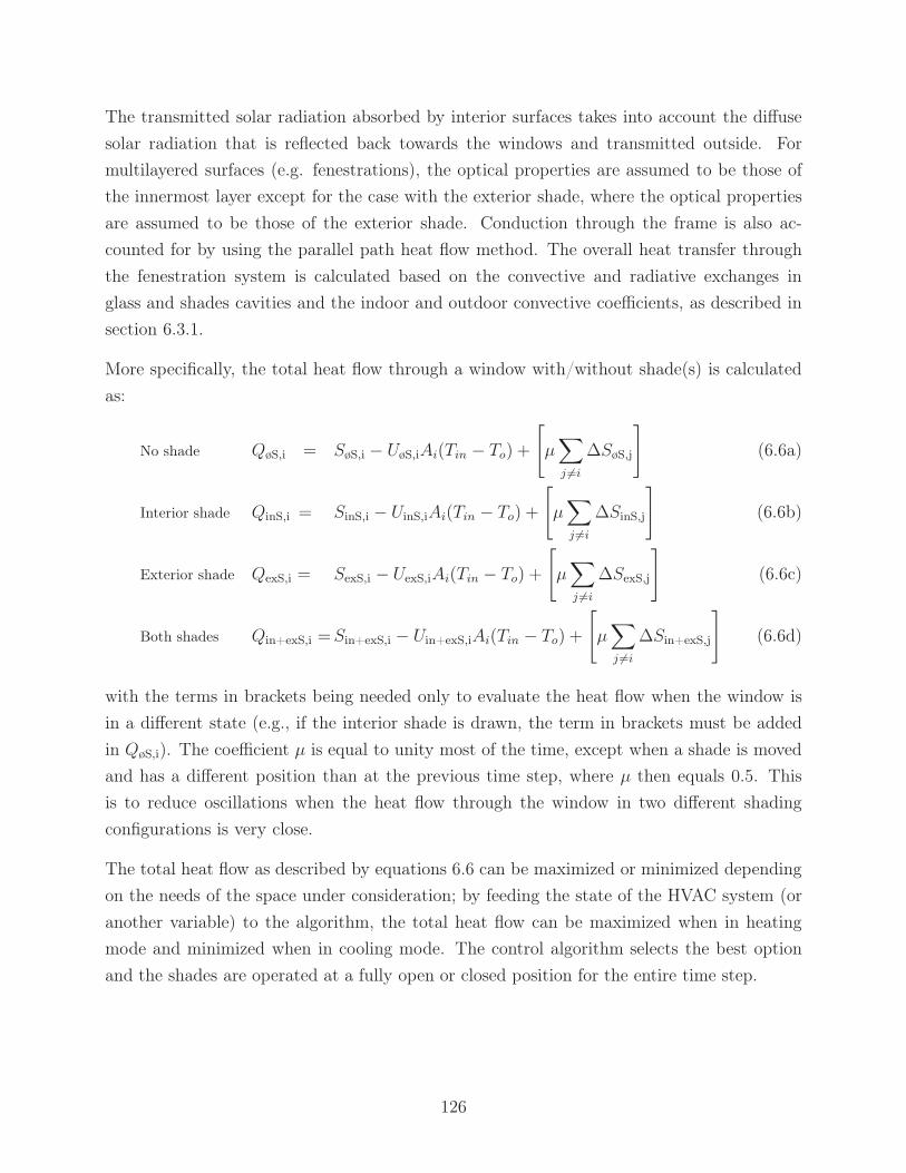
The transmitted solar radiation absorbed by interior surfaces takes into account the diffuse

solar radiation that is reflected back towards the windows and transmitted outside. For

multilayered surfaces (e.g. fenestrations), the optical properties are assumed to be those of

the innermost layer except for the case with the exterior shade, where the optical properties

are assumed to be those of the exterior shade. Conduction through the frame is also ac-

counted for by using the parallel path heat flow method. The overall heat transfer through

the fenestration system is calculated based on the convective and radiative exchanges in

glass and shades cavities and the indoor and outdoor convective coefficients, as described in

section 6.3.1.

More specifically, the total heat flow through a window with/without shade(s) is calculated

as:

No shade QøS,i = SøS,i − UøS,iAi(Tin − To) +

[μ

∑j �=i

ΔSøS,j

](6.6a)

Interior shade QinS,i = SinS,i − UinS,iAi(Tin − To) +

[μ

∑j �=i

ΔSinS,j

](6.6b)

Exterior shade QexS,i = SexS,i − UexS,iAi(Tin − To) +

[μ

∑j �=i

ΔSexS,j

](6.6c)

Both shades Qin+exS,i =Sin+exS,i − Uin+exS,iAi(Tin − To) +

[μ

∑j �=i

ΔSin+exS,j

](6.6d)

with the terms in brackets being needed only to evaluate the heat flow when the window is

in a different state (e.g., if the interior shade is drawn, the term in brackets must be added

in QøS,i). The coefficient μ is equal to unity most of the time, except when a shade is moved

and has a different position than at the previous time step, where μ then equals 0.5. This

is to reduce oscillations when the heat flow through the window in two different shading

configurations is very close.

The total heat flow as described by equations 6.6 can be maximized or minimized depending

on the needs of the space under consideration; by feeding the state of the HVAC system (or

another variable) to the algorithm, the total heat flow can be maximized when in heating

mode and minimized when in cooling mode. The control algorithm selects the best option

and the shades are operated at a fully open or closed position for the entire time step.

126

A thermal network showing the conductive, radiative and convective heat transfers in the

fenestration system considered in this study is shown in figure 6.8. Convective and radiative

coefficients hc,i and hr,i are calculated individually at every time step as described in sections

6.3.1.3 and 6.3.1.4.

��

�������

����� ��������� ����

��������� ��������� ��������

� ����

� ������

����� ������

����� �����

��� ���

������� �������������

����

��

Figure 6.8: Thermal network of a fenestration system

From a physical point of view, maximizing or minimizing the total heat through a fenestration

system, as described by the four discrete feasible solutions from equations 6.6, is rather

straightforward. The difficulties reside in the numerical modelling, as many what if scenarios

must be considered.

Calculating the heat flow through a bare window is simple. Calculating the heat flow through

that window if a shade was drawn requires the calculation of the shade temperature if it was

present because the convective and radiative heat transfer depend on it. Therefore, at all

time steps, the temperature of the shade(s) must be calculated, whether present or not.

Another difficulty arises by the fact that drawing a shade of one window affects not only

the solar gains through that window but also from other windows. For instance, in early

morning, opening the east shade allows the solar gains inside the space and closing the west

shade contributes to keeping these gains inside the space (opening the west shade would allow

most beam radiation to escape the space). Therefore, at all time steps, it is necessary to

calculate not only the solar radiation transmitted by surface i and absorbed with the actual

shade(s) position, but also the absorbed radiation change if a shade is closed (or opened), for

all glazed orientations. This is represented by the terms in brackets in equations 6.6.

127

6.5.3 Simulation results and discussion

The main objective of these simulations is to compare different types of controls for motorized

shadings and assess their relative energy performance. An energy efficient solarium design was

selected with the goal of collecting surplus heat that could be used to heat the adjacent house.

Annual simulations were performed for the city of Montreal from October 1st to September

30th with a 28 days simulation warm-up period. The year is divided in two modes : a

heating mode (October 1st to April 30th) and a mixed mode (May 1st to September 30th).

During the heating mode, excess energy was considered when the temperature reached 28°C

and heating is provided to keep a minimum temperature of 10°C. This surplus heat could be

stored (with more thermal storage) or transferred to the house to partly offset its heating

load.

The energy control algorithm is detailed is section 6.5.2. This type of control is compared

with a control scheme based on a fixed solar radiation set-point. For the solar control scheme,

shades are controlled together based on the global horizontal solar radiation level; they open

when this level exceeds a predetermined value. Many simulations were run with different

solar radiation levels at 25 W/m2 increments, but only the best results are presented in table

6.4. Therefore, these radiation levels can be considered as near optimum. The solar radiation

set-point judged the best was the one providing the highest average temperature during the

heating mode. These set-points are presented in bold in table 6.4 and all comparisons are

performed in regards to these best solar radiation set-points.

During the heating mode, the energy control algorithm is set to maximize the total heat

flow at all time. During the mixed mode, the energy control algorithm minimizes the heat

flow if the inside temperature is above 25°C or maximizes it otherwise. For the solar control

in mixed mode, in addition to open when the global horizontal solar radiation level exceeds

a chosen value, all shades are closed if the inside temperature is above 25°C. For all shade

control types, there is no controlled ventilation in heating mode and there is 2 air change per

hour if the inside temperature is above 23°C in mixed mode.

6.5.3.1 Energy consumption

As seen from table 6.4, the heating consumption of a solarium with an interior shade con-

trolled with the energy scheme can be reduced by 3% compared to a control based on a global

solar radiation level of 50 W/m2. In addition, the excess energy (i.e. the heat stored when

the temperature inside the solarium reached 28°C) can be increased by 10%.

128

Table 6.4: Heating requirements, excess energy, average temperature and percentage ofcomfortable hours of a solarium with clear double glazing and different shade configurationsand controls (Set-points in heating mode: 10-28°C)

Type of control Heating Excess Average Comfort Average ComfortkWh energy temperature time temperature time

kWh °C % °C %Heating mode Mixed mode

Solarium without shades

No shades 3011 656 15.47 31.0 27.17 43.3

Solarium with interior shade

Energy balance 1856 1338 17.53 35.9 26.33 63.3Solar (25W/m2) 1897 1184 17.38 35.8 27.43 42.5Solar (50W/m2) 1921 1214 17.41 35.7 27.44 42.5Solar (75W/m2) 1991 1234 17.39 35.7 27.44 42.6

Solarium with exterior shade

Energy balance 1222 1216 17.61 36.1 24.25 97.7Solar (25 W/m2) 1324 1091 17.33 36.1 24.35 97.8Solar (50 W/m2) 1313 1111 17.39 36.0 24.35 97.8Solar (75 W/m2) 1349 1120 17.39 35.8 24.36 97.8

Solarium with interior and exterior shade

Energy balance 670 2007 19.25 34.7 24.65 97.9Solar (25-50 W/m2) 767 1670 18.88 35.6 24.73 98.3Solar (50-50 W/m2) 735 1756 18.98 35.5 24.75 98.3Solar (50-75 W/m2) 780 1760 18.94 32.3 24.74 98.3

For a solarium with an exterior shade, the heating consumption can be reduced by 7% and

the excess energy can be increased by 9% with the proposed control strategy compared to a

radiation set-point of 50 W/m2.

For a solarium design with both interior and exterior shades, the heating consumption can

be reduced by 9% and the excess energy can by increased by 14% compared to a radiation

set-point of 50 W/m2 for both shades.

The solarium has a significantly lower heating consumption when equipped with an exterior

shade compared to an indoor one. This is due to the increased thermal resistance of the

exterior shade. However, the solarium equipped with an interior shade can collect more

surplus heat than with an exterior shade, because of its higher solar transmittance.

129

6.5.3.2 Thermal comfort

A common desirable feature of a solarium is to connect its occupants with the exterior

surrounding. Given the nature of this space, a wider temperature range than usual was

selected for the thermal comfort range. The lowest limit for thermal comfort has been

selected as 17°C, as it represents the lowest acceptable temperature (with 80% acceptance) for

naturally ventilated buildings with a mean outdoor temperature of 5°C. The upper limit for

comfort has been selected as 28°C. It should be remembered that the indoor air temperature

was not allowed to go above 28°C when in heating mode.

The percentage of time when the operative temperature was within the comfort zone as

described above is presented in table 6.4. When the exterior shade is controlled with the en-

ergy scheme, either alone or in combination with the interior shade, the comfortable period

is similar to other control types. The exterior shade, which is opaque to solar radiation, is

highly effective for limiting temperature rise, regardless of the control type. Controlling the

interior shade with the energy scheme during the mixed mode reduces the average tempera-

ture by 1.1°C and yields 20.8% more comfortable hours, which represents 1822 hours during

the simulated period.

6.6 Applications, recommendations and limitations

The shading control strategy proposed here can be used in solariums and greenhouses as well

as residential and office buildings. In all cases, the presence of thermal storage materials is

important for maximizing the energy gains obtained by using this control strategy, especially

during the heating and shoulder periods.

One proven method of enhancing solar gain utilization is by integrating thermal storage ma-

terials in direct-gain rooms. In buildings with large glazed area, the solar gains often exceed

the instantaneous heating load during the shoulder seasons; significant amounts of thermal

mass are thus required to store the excess solar gains without causing large temperature

swings (Athienitis et al., 1997).

This control algorithm can be used for minimizing or maximizing the total heat flow through

fenestrations systems; therefore, it can be used in both heating and cooling modes. The

switch from one state to another can be triggered by feeding the state of the HVAC system

to the algorithm, the indoor or outdoor temperature, or other user-defined criteria.

130

The proposed control strategy can be employed in solariums and greenhouses in all climate

types. Attached solariums and rooftop greenhouses can transfer the surplus heat to the

adjacent building, thus maximizing the energy gains by making use of the excess heat. For

old houses, the excess heat is likely to be useful at all time during the heating season, but this

might not be the case for more recent houses with a better envelope (Bastien and Athienitis,

2013).

This control strategy is also applicable to greenhouses, where it can be particularly useful for

closed and semi closed greenhouses. A closed greenhouse has no openings to bring in fresh

air for humidity and temperature control. It is equipped with a seasonal thermal storage,

where heat is stored during the summer for use in winter. In addition, dehumidification

equipment must be present for humidity control (Vadiee and Martin, 2012). Typically, a

closed greenhouse can collect about four times the heat needed for its winter operation during

one year. Therefore, some are suggesting to build one closed greenhouse in combination to

three normal greenhouses to fully utilize the solar gains (Vadiee and Martin, 2013a).

Closed greenhouses require a lot of mechanical equipment for temperature and humidity

control, making them relatively expensive to build and operate. As a more viable alter-

native, the semi closed greenhouse concept has been suggested where part of the cooling

and dehumidification demand is met by ventilation through windows (Vadiee and Martin,

2012).

Implementing the control algorithm presented here for maximizing the heat flow in closed

greenhouses would make use of the excess heat all year round by either using it or storing

it. Implementing it in semi closed and conventional greenhouses in both heating and cool-

ing modes could reduce the heating requirements when in heating mode and reduce indoor

temperature when in cooling mode.

This shading control strategy can also be applicable to residential buildings for maximizing

the solar energy utilization from glazed surfaces. For applications like a solarium or a house

where providing living space for occupants is important, the proposed control algorithm could

be implemented as the default mode while allowing occupants override to provide for glare

and privacy issues.

This control algorithm can also be included as an additional criteria in existing control

strategies for office buildings based on visual comfort. Depending on the state of the HVAC

system, equations 6.6 can be maximized or minimized to reduce the heating and cooling

loads. The internal gains from the lighting system can be easily added to equations 6.6 so as

to define a control strategy that utilizes daylight but does not allow excessive solar gains, such

131

as the approach suggested by Tzempelikos and Shen (2013). Optimal control algorithms such

as the one presented in Kummert et al. (2001) where a cost function depending on heating

consumption and thermal comfort is minimized should be developed for the optimal control of

shades, lights and HVAC systems to reduce the overall energy consumption while maintaining

thermal and visual comfort. The method presented in this chapter for calculating the total

heat flow through fenestration systems could be useful for reaching this goal.

6.7 Conclusion

This paper presents a new control strategy for improving the control of shades based on

performing an energy balance on fenestration systems. Difficulties associated with the nu-

merical implementation of this control strategy are discussed and solutions are proposed.

The presented control algorithm is generic and can be applied to any glazing type, shad-

ing properties, façade orientation and climate. It is suitable for spaces with multiple façade

orientations.

The control strategy is based on analyzing the total heat flow, which can be maximized or

minimized depending on the needs of the space. The presented control strategy can be used

with one interior and/or one exterior planar shade.

This control method could be useful for solariums, greenhouses and residential buildings.

It could also be included as an additional criteria in existing control strategies for office

buildings.

A solarium model was developed in order to assess the performance of the proposed shading

strategy. The simulation model has been compared experimentally with a prototype solarium

equipped with indoor and outdoor motorized shadings and a ventilated thermal storage wall

with phase change materials. Numerical simulations are in good agreement with experimental

results.

Using this model, annual energy simulations of a solarium have been performed for the

location of Montreal, Canada. The year has been divided in a heating mode (October to

April) and a mixed mode (May to September). Results for heating mode indicate that the

proposed control method can reduce the heating consumption by 3% and 7% for an interior

and exterior shade, respectively. In addition, the excess heat collected can be increased by

10% and 9% for an interior and exterior shade, respectively. When using both an indoor and

outdoor shade, the proposed control could reduce heating by 9% and increase the excess heat

132

collected by 14%. Results for the mixed mode show that operating the interior shade with

the proposed control can significantly improve thermal comfort by increasing the comfortable

period from 42.5% to 63.3%, which corresponds to 1822 hours.

Future research should include evaluating the performance of this shading control strategy

for other building and shading types; developing a methodology for selecting high performing

fenestration systems (i.e. combination of glazing with shades); and quantifying the benefits

of different thermal mass levels in solariums and greenhouses.

133

Chapter 7

Methodology for sizing passive thermal

energy storage in solaria and

greenhouses

7.1 Chapter abstract

This paper presents a methodology for sizing passive thermal energy storage (TES) systems

in solaria and greenhouses. First, potential targets for thermal mass design strategies are

reviewed, along with common metrics used in the characterization of the performance of TES

systems. This review exercise of targets and metrics provides the basis for the identification

of the most relevant performance variables for solaria and greenhouses.

Six different solarium/greenhouse designs are investigated, which encompass the most fre-

quent configurations. These configurations are studied with two complementary approaches:

frequency response (FR) and finite difference thermal network (FD). FR models are used

for sensitivity studies under short periodic design sequences while FD models are used in

full-year performance assessments with real weather data.

Finally, a methodology for sizing TES in solaria and greenhouses is presented along with

design recommendations. The energy balance equations for six different configurations are

included, thereby the methodology is applicable to a variety of designs. The methodology is

based on a FR model with a simulation design period of five cold sunny days followed by five

cold cloudy days; such a design period proved to be representative of the harshest conditions

in a year and thus provides a good basis for assessing design improvements. Simulation

134

results obtained with the FR and FD models showed a significant reduction of the daily

operative temperature swing in the presence of a TES up to a thickness of 0.15-0.20 m

where it remained mostly constant beyond. Increasing the thickness of a TES from 0.10

to 1 m was shown to raise the minimum operative temperature by 3 to 5 °C in unheated

solaria/greenhouses. If providing comfort during the evening is an important design goal, a

design with opaque north, east and west walls should be selected and include one TES on

the floor or the north wall 0.05-0.10 m thick or two TES on both the wall and the floor with

a thickness close to 0.06 m.

7.2 Introduction

Thermally massive elements have been present in vernacular architecture for hundreds of

years; they were indeed necessary to limit temperature fluctuations and provide relative

comfort in buildings before fossil fuels became largely available (Rempel and Rempel, 2013).

Faced with a limited supply of fossil resources and climate change, thermal energy storage

(TES) systems are still attracting interest nowadays. Storage of thermal energy is important

in many applications, and especially for solar energy systems (Hasnain, 1998).

Massive materials have the ability absorb heat and release it later; the timing of the peak

heat delivery should be optimized depending on the building type under consideration. For

instance, Rempel and Rempel (2013) suggest 1) evening space heating for people at home;

2) afternoon space heating for people at work or at school; 3) all-night space heating for

plants; 4) daytime space cooling for people, plants or equipment. They note that while

passive systems cannot deliver instantly heat or cooling like mechanical systems, they are

nevertheless highly adjustable by varying their material, thickness and configuration.

Many studies have been conducted about the energy saving potential of various TES designs,

and a very large range of saving is reported, from being negligible up to 90% of space heating

reduction (Burns et al., 1991; Kosny et al., 2001; Parameshwaran et al., 2012). This vari-

ability is caused not only by the wide design possibilities of TES systems, but also because

their performance is strongly linked to their operational characteristics. While most studies

identified that TES can significantly reduce the peak heating and cooling loads, a significant

number of studies reported little energy savings attributed to TES (Bojic and Loveday, 1997;

Aste et al., 2009; Ozel, 2014; Navarro et al., 2015).

135

As reported by MacCracken (2003), even if a building equipped with a TES is only shifting

a portion of it’s energy consumption from on-peak to off-peak hours but has the same total

energy consumption, source energy savings will occur – which are 8% to 30% for two of the

major California utilities. They pointed out that pollutant emissions will also be reduced,

since power plants used for peak demand are the dirtiest.

The integration of TES in buildings is of particular interest for improving user acceptance

(Navarro et al., 2015). Buildings integrated with TES (BITES) can be classified as active

or passive systems, or a combination of both. No mechanical equipment is used in passive

systems while active systems use fluids for exchanging heat with the storage media. Passive

TES systems can be included in buildings at little or no cost and have the added advantages

of the simplicity of design, operation and maintenance (Tiwari et al., 1988). This study is

focusing on passive TES.

7.2.1 Control of passive thermal energy storage

Yu et al. (2015) presented a review of control strategies employed with active and passive

BITES. They noted that buildings with passive BITES are usually equipped with HVAC

systems and other equipment for regulating indoor air temperature and that an effective

strategy for their control can help to maximize energy savings associated with BITES. As

mentioned by Hasnain (1998), the use of inertia in building mass does not require additional

HVAC equipment but special controls are required. Yu et al. (2015) noted a lack of studies on

developing and evaluating control strategies for HVAC and other systems with the different

types of passive BITES and concluded that future research is needed in this area.

As stated by (Bojic and Loveday, 1997), it is very important to know if the building will be

heated or cooled on an intermittent or continuous basis when designing the building mass for

energy savings. However, this aspect is often neglected with the majority of studies employing

fixed thermostat set-points for the entire duration of the heating and cooling seasons.

An extensive study of lightweight and massive residential buildings located in various loca-

tions in the United States found that energy savings resulting from replacing light weight

walls with heavy constructions are very location specific: they found reductions up to 8% of

heating energy in Minneapolis and up to 18% cooling energy in Bakersfield, California (Kosny

et al., 2001). Although not mentioned in the study, the set-points for heating and cooling

were probably constants, indicating that further savings could be possible with different

temperature controls.

136

A study about the impacts of thermal inertia in buildings found that the potential reduction in

the energy used for heating and cooling is strongly linked to the building operation parameters

such as ventilation rates and set-points for heating and cooling (Aste et al., 2009). Numerical

simulations of a large building with EnergyPlus have shown that a reduction of 10% of heating

energy and 20% of cooling energy is achievable in Milano by using materials with high thermal

inertia coupled with appropriate operational characteristics. However, their simulations also

showed that savings can be nil in the absence of adequate operational measures, like in the

absence of natural ventilation at night for saving cooling energy.

According to Heier et al. (2015), sensible passive TES may pursue two objectives: either to

maximize energy savings or improve thermal comfort. Since large swings of indoor temper-

ature are beneficial for energy savings and a narrow temperature interval is key to thermal

comfort, these two objectives are in conflict. This conflict may be alleviated when using phase

change materials (PCM) since these materials can exchange heat effectively within a narrow

temperature interval. This review identified that for residential buildings, most research have

showed that only a small reduction of the heating demand is possible when using passive TES,

either sensible or latent. Since TES need temperature variations to work efficiently as ther-

mal storage, this might be the result of the strictly controlled lowest allowable temperature

in residential buildings, which leaves little room for heating energy savings.

7.2.2 Design approaches

Several design approaches have been considered for the capture and release of solar heat: 1)

massive exterior wall; 2) Trombe wall; 3) direct-gain space; and 4) isolated-gain space.

Massive exterior walls have been used for centuries, mainly in the form of thick adobe, cob or

stone walls used in traditional architecture. Trombe walls introduced a glazed layer in front of

the massive wall, mainly for reducing heat losses. Direct-gain spaces allow solar heat to enter

in living spaces through windows and store that heat in interior massive elements, usually

the floor or walls. Balcomb (1983) reported that it was previously thought that the thermal

mass had to be exposed to direct sun to be effective, but notes that most massive surfaces

enclosing a direct-gain space are quite effective as well. Isolated-gain spaces are similar to

direct-gain spaces but are free of the requirement of maintaining thermal comfort for people.

They may need adequate conditions for protecting plants, but their thermal requirements are

more flexible than for normally conditioned spaces. This paper is focused on isolated-gain

spaces such as solaria and greenhouses.

137

7.2.3 The use of passive storage in solaria and greenhouses: a re-

view

Many solaria and greenhouses with various passive TES materials have been simulated and

built. The most studied TES design consists of a thermally massive north wall. Since solar

radiation incident from a south glazing can easily escape through the north glazing, the north

wall is better opaque and insulated. Accordingly, the north wall becomes a privileged location

for thermal mass. An example of the diversity of the materials and configurations selected

as a north wall TES in solaria and greenhouses and their influence on the indoor climate is

reported in Table 7.1.

China has a long tradition of local cultivation using so-called chinese solar greenhouses (CSG).

In 2000, there were more than 2600·106 m2 of CSG being used, providing more than 90% of

the vegetables consumed in northern China in winter (Tong et al., 2009). These greenhouses

have all adopted a similar design with a plastic film covering the slanted south roof, a ther-

mal blanket deployed at night and a thermally massive north wall. These greenhouses are

inexpensive and generally built with local materials. Examples of TES in CSG are reported

in Table 7.1, where we can see that some earth walls can be as thick as 550 cm. Earth walls

are usually rammed, either manually or mechanically, where machine rammed earth walls

have a trapezoidal cross section with a smaller section at the top.

As reported by Tong et al. (2013), a few studies of massive north walls in CSG all concluded

that when insulated, the best performance occurs when the insulation layer is on the outside of

the massive layer; this finding is similar to studies conducted with other building types.

Wang et al. (2014) carried out simulations of CSG with different north wall designs. They

mentionned that a thick earth wall can be conceptually divided into three layers: the energy-

storing layer (inside), the thermally stable layer (in the middle) and the thermal insulating

layer (outside). Their simulations carried out under winter conditions in northern China

revealed that a 1 m wall has no thermally stable layer while this layer comprised 23% of

the cross sectional area of a 1.5 m wall. From optimization calculations for minimizing the

cross sectional area and maintaining a minimum temperature above 10 °C, they suggest a

design of a trapezoidal wall 1.7 m thick at the base and 0.5 m thick at the top. They also

conducted an analysis of the minimum air temperature as a function of the total thermal

resistance and the thermal inertia index. They observed that the minimum temperature

increases with both parameters, with a slower increasing rate with further increases of these

two parameters.

138

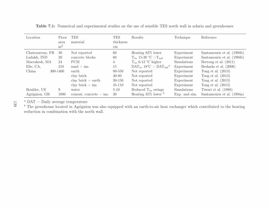
Table 7.1: Numerical and experimental studies on the use of sensible TES north wall in solaria and greenhouses

Location Floor TES TES Results Technique Referencearea material thicknessm2 cm

Chateauroux, FR 30 Not reported 60 Heating 82% lower Experiment Santamouris et al. (1994b)Ladakh, IND 20 concrete blocks 60 Tin 15-20 °C >Tout Experiment Santamouris et al. (1994b)Marrakesh, MA 24 PCM 4 Tin 6-12 °C higher Simulations Berroug et al. (2011)Elie, CA, 210 sand + ins. 15 DATin 18°C > DATout

a Experiment Beshada et al. (2006)China 300-1400 earth 80-550 Not reported Experiment Tong et al. (2013)

clay brick 40-80 Not reported Experiment Tong et al. (2013)clay brick + earth 30-150 Not reported Experiment Tong et al. (2013)clay brick + ins. 45-110 Not reported Experiment Tong et al. (2013)

Boulder, US 9 water 5-10 Reduced Tin swings Simulations Tiwari et al. (1988)Agrignion, GR 1000 cement, concrete + ins. 30 Heating 35% lower b Exp. and sim. Santamouris et al. (1994a)

a DAT = Daily average temperatureb The greenhouse located in Agrignion was also equipped with an earth-to-air heat exchanger which contributed to the heatingreduction in combination with the north wall.

139

In a redesign study of a solarium located in Oregon, U.S., Rempel et al. (2013) compared the

performance of integrating different levels of TES. They noticed lower air temperature peaks

and warmer minimum air temperature for designs with a high level of TES. However, they

also noted a slightly lower average temperature and less heat retained during the heating

season than for a medium level of TES, and thus suggest to avoid the oversizing of TES.

They report that occupants prioritized the experience of early evening warmth and plant

protection over the supply of heat for living spaces. Interestingly, as shown later in this

paper, these two priorities calls for two different thermal mass design.

Numerical and experimental studies have been conducted on the performance of greenhouses

using seasonal energy storage (Vadiee and Martin, 2013b; Xu et al., 2014; Zhang et al.,

2015). For efficient heat delivery and lower costs, these systems are usually equipped with

a short term storage and a long term storage. Greenhouses using seasonal TES rely on

active components for transferring heat from the storage media to the greenhouse air and are

therefore outside the scope of this paper.

7.2.4 Objectives and overview

The aim of this contribution is to present a methodology for assisting in the design of passive

TES for solaria and greenhouses. Different objectives may be pursued by incorporating

TES in buildings; they are reviewed in section 7.3, along with commonly used metrics for

characterizing the performance of TES. From this review, the most relevant performance

metrics for isolated-gain applications are highlighted.

Six general solarium/greenhouse designs are investigated in this study and presented in sec-

tion 7.4, which encompass the most frequent configurations. These configurations are an-

alyzed with two complementary numerical modelling methods: one based on a frequency

response (FR) approach for the analysis of design sequences and one based on a thermal

network model solved with the finite difference (FD) method for yearly analysis.

With the FR method presented in section 7.5, different design periods are examined along

with their impact on the optimal thickness of thermal storage. The effect of glazing type,

varying floor area and aspect ratio, varying thermal resistance of the insulation layer, increas-

ing thermal coupling (by raising indoor air circulation), varying thermal storage material and

different design periods on the main performance variables is investigated.

The FD method, which requires spatial discretization of the thermal mass, is detailed in

section 7.6. First, results obtained with the FR model are used to assist in the determination

140

of important parameters needed for the FD model, such as the number of nodes needed for

the discretization of thermal mass. The effect of using constant, linear or non linear radiative

and convective coefficients is assessed. Then, the FD method is using real weather data for

analyzing the behavior of the investigated configurations for a complete year. The amount of

storage needed for reaching different design goals is investigated. Both heated and unheated

spaces are analyzed. The performance is evaluated for two different years and canadian

cities, which allows the assessment of the sensitivity of the TES design to varying climatic

conditions.

Finally, the proposed methodology for sizing TES, based on the FR model, is detailed in

section 7.7 and design recommendations are presented in section 7.8.

7.3 Design intents behind thermal mass design strate-

gies

When designing thermally massive elements in buildings, many objectives may be pursued,

such as: 1) delaying the peak solar gain effect to a more favorable moment; 2) reducing the

peak heat flux or the peak temperature at the room-facing layer; 3) reducing the space heating

energy consumption; 4) reducing the temperature swings; 5) increasing the average space

temperature; 6) increasing the minimum temperature or reducing the maximum temperature.

One may focus on the processes (i.e. heat fluxes) or on the results (i.e. temperatures).

Sometimes, these objectives will be in conflict with each other and call for different materials

and configurations; therefore a designer must carefully select the objectives to be prioritized

for a given application.

This section reviews different metrics associated to the six objectives enumerated above and

discusses their relevance for passive TES in isolated-gain applications.

7.3.1 Optimal time lag

In many thermal mass design studies, the time lag is defined as the delay between the

moment when the outer surface and the inner surface of an external wall reach their peak

temperatures (τ[Tpeak]). Many studies have analyzed the distribution and thermophysical

properties of thermal mass and insulation layers of exterior walls and their impact on τ[Tpeak]

and the decrement factor (the decrement factor is discussed in the next subsection). Most

141

studies present their analysis based on identifying the optimum distribution or properties

for maximizing the peak temperature time lag and minimizing the decrement factor (Asan,

2000; Ulgen, 2002; Ozel and Pihtili, 2007; Ibrahim et al., 2013; Jin et al., 2012; Evola and

Marletta, 2013). However, as explained below, these two objectives are not appropriate for

isolated-gain applications.

Asan (2000) presented a numerical study on the investigation of the wall’s optimum insulation

position in terms of maximum peak temperature time lag and minimum decrement factor.

He found that placing half the insulation in the middle of the wall and the other half at the

outer surface provides both very high lag time and low decrement factor – close to optimum

values.

However, as noted by Rempel and Rempel (2013), the timing of the peak heat delivery should

actually depend on the building type and needs. The time lag can easily exceed 12 hours for

many materials with a thickness of 30 cm and even exceed 24 hours (Asan, 2006). When the

heat flux input is from solar radiation, a time lag of 24 hours in fact means no time lag at all;

therefore the common conception that maximizing the time lag yields optimal performance

should be reconsidered.

Some studies assumed a sinusoidal sol-air temperature over a 24 hour period (Asan, 2006).

However, day length is 12 hours only at the equinox; therefore, a more realistic sol-air tem-

perature profile should be employed for winter conditions by using Fourier series. When the

sol-air temperature is calculated with more than 1 harmonic (i.e. not simply sinusoidal), the

time lag of the temperature peaks and temperature crests are also different (Sun et al., 2013;

Kontoleon and Bikas, 2007).

Sun et al. (2013) observed that for a massive exterior wall exposed to various periodic condi-

tions, the average of the temperature peak and crest time lag is equal to the time lag under

a sinusoidal input. The analysis of their results revealed that with a difference between the

peak and crest time lag of up to 3.5 h, estimating the time lag under a sinusoidal input could

induce a difference of 1.75 h with the peak time lag; this result highlights the importance of

using non sinusoidal profiles as input sources.

As noted by Kontoleon and Bikas (2007), evaluating τ[Tpeak] is especially important during the

cooling season for buildings that can use natural ventilation for night cooling. Gagliano et al.

(2014) reported that many designers tend to increase thermal inertia without considering their

limits and proper applications. They suggest that east walls should have time lags about 12-

14 hours while it should be around 8 hours for west walls; longer time lags would be counter

productive since that would reduce the useful time for exploiting night ventilation.

142

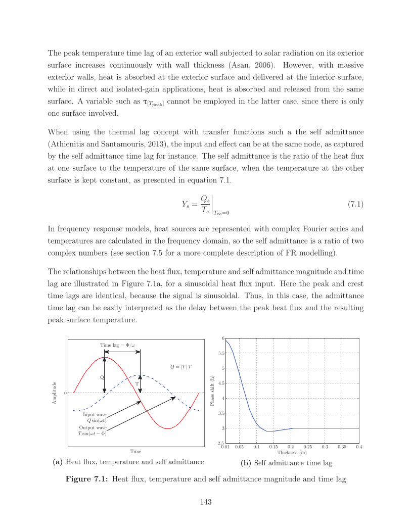
The peak temperature time lag of an exterior wall subjected to solar radiation on its exterior

surface increases continuously with wall thickness (Asan, 2006). However, with massive

exterior walls, heat is absorbed at the exterior surface and delivered at the interior surface,

while in direct and isolated-gain applications, heat is absorbed and released from the same

surface. A variable such as τ[Tpeak] cannot be employed in the latter case, since there is only

one surface involved.

When using the thermal lag concept with transfer functions such a the self admittance

(Athienitis and Santamouris, 2013), the input and effect can be at the same node, as captured

by the self admittance time lag for instance. The self admittance is the ratio of the heat flux

at one surface to the temperature of the same surface, when the temperature at the other

surface is kept constant, as presented in equation 7.1.

Ys =Qs

Ts

∣∣∣∣Teo=0

(7.1)

In frequency response models, heat sources are represented with complex Fourier series and

temperatures are calculated in the frequency domain, so the self admittance is a ratio of two

complex numbers (see section 7.5 for a more complete description of FR modelling).

The relationships between the heat flux, temperature and self admittance magnitude and time

lag are illustrated in Figure 7.1a, for a sinusoidal heat flux input. Here the peak and crest

time lags are identical, because the signal is sinusoidal. Thus, in this case, the admittance

time lag can be easily interpreted as the delay between the peak heat flux and the resulting

peak surface temperature.

Time

Am

plit

ude

Time lag = Φ/ω

QT

Input waveQ sin(ωt)

Output waveT sin(ωt − Φ)

Q = |Y |T

0

(a) Heat flux, temperature and self admittance

Thickness (m)

Pha

sesh

ift

(h)

0.01 0.05 0.1 0.15 0.2 0.25 0.3 0.35 0.42.5

3

3.5

4

4.5

5

5.5

6

(b) Self admittance time lag

Figure 7.1: Heat flux, temperature and self admittance magnitude and time lag

143

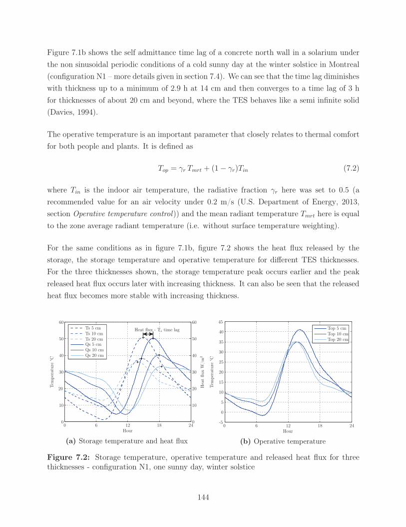
Figure 7.1b shows the self admittance time lag of a concrete north wall in a solarium under

the non sinusoidal periodic conditions of a cold sunny day at the winter solstice in Montreal

(configuration N1 – more details given in section 7.4). We can see that the time lag diminishes

with thickness up to a minimum of 2.9 h at 14 cm and then converges to a time lag of 3 h

for thicknesses of about 20 cm and beyond, where the TES behaves like a semi infinite solid

(Davies, 1994).

The operative temperature is an important parameter that closely relates to thermal comfort

for both people and plants. It is defined as

Top = γr Tmrt + (1 − γr)Tin (7.2)

where Tin is the indoor air temperature, the radiative fraction γr here was set to 0.5 (a

recommended value for an air velocity under 0.2 m/s (U.S. Department of Energy, 2013,

section Operative temperature control)) and the mean radiant temperature Tmrt here is equal

to the zone average radiant temperature (i.e. without surface temperature weighting).

For the same conditions as in figure 7.1b, figure 7.2 shows the heat flux released by the

storage, the storage temperature and operative temperature for different TES thicknesses.

For the three thicknesses shown, the storage temperature peak occurs earlier and the peak

released heat flux occurs later with increasing thickness. It can also be seen that the released

heat flux becomes more stable with increasing thickness.

Hour

Tem

per

atur

e°C

Hea

tflu

xW

/m2

Ts 5 cmTs 10 cmTs 20 cmQs 5 cmQs 10 cmQs 20 cm

Heat flux - Ts time lag

0

0 6 12 18 240

10

20

30

40

50

60

0

10

20

30

40

50

60

(a) Storage temperature and heat flux

Hour

Tem

per

atur

e°C

Top 5 cmTop 10 cmTop 20 cm

0 6 12 18 24-5

0

5

10

15

20

25

30

35

40

45

(b) Operative temperature

Figure 7.2: Storage temperature, operative temperature and released heat flux for threethicknesses - configuration N1, one sunny day, winter solstice

144

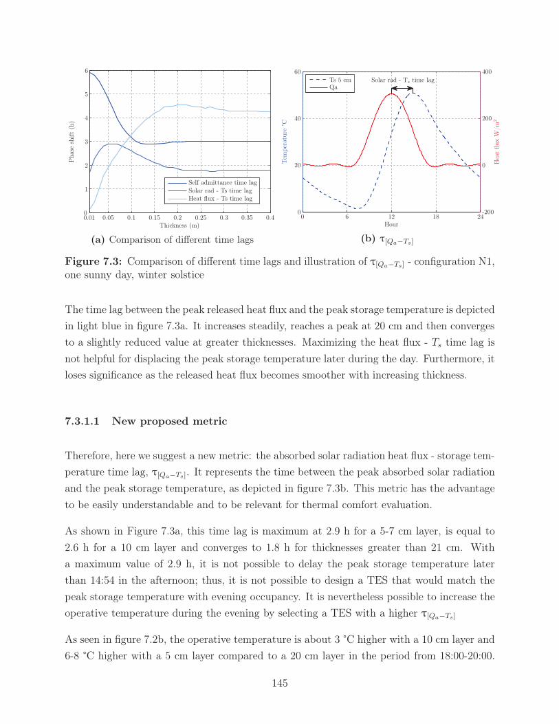
Thickness (m)

Pha

sesh

ift

(h)

Self admittance time lagSolar rad - Ts time lagHeat flux - Ts time lag

0.01 0.05 0.1 0.15 0.2 0.25 0.3 0.35 0.40

1

2

3

4

5

6

(a) Comparison of different time lags

Hour

Tem

per

atur

e°C

Hea

tflu

xW

/m2

Ts 5 cmQa

Solar rad - Ts time lag

0 6 12 18 24-200

0

200

400

0

20

40

60

(b) τ[Qa−Ts]

Figure 7.3: Comparison of different time lags and illustration of τ[Qa−Ts] - configuration N1,one sunny day, winter solstice

The time lag between the peak released heat flux and the peak storage temperature is depicted

in light blue in figure 7.3a. It increases steadily, reaches a peak at 20 cm and then converges

to a slightly reduced value at greater thicknesses. Maximizing the heat flux - Ts time lag is

not helpful for displacing the peak storage temperature later during the day. Furthermore, it

loses significance as the released heat flux becomes smoother with increasing thickness.

7.3.1.1 New proposed metric

Therefore, here we suggest a new metric: the absorbed solar radiation heat flux - storage tem-

perature time lag, τ[Qa−Ts]. It represents the time between the peak absorbed solar radiation

and the peak storage temperature, as depicted in figure 7.3b. This metric has the advantage

to be easily understandable and to be relevant for thermal comfort evaluation.

As shown in Figure 7.3a, this time lag is maximum at 2.9 h for a 5-7 cm layer, is equal to

2.6 h for a 10 cm layer and converges to 1.8 h for thicknesses greater than 21 cm. With

a maximum value of 2.9 h, it is not possible to delay the peak storage temperature later

than 14:54 in the afternoon; thus, it is not possible to design a TES that would match the

peak storage temperature with evening occupancy. It is nevertheless possible to increase the

operative temperature during the evening by selecting a TES with a higher τ[Qa−Ts]

As seen in figure 7.2b, the operative temperature is about 3 °C higher with a 10 cm layer and

6-8 °C higher with a 5 cm layer compared to a 20 cm layer in the period from 18:00-20:00.

145

This result showcases the value of τ[Qa−Ts] as an index: a higher value indicates improved

thermal comfort later in the day, although at the cost of lower morning temperatures.

In light of these observations, it is clear that τ[Qa−Ts] is a valuable index for indirect-gain

spaces and will therefore be one of the key output variables analyzed in this paper.

7.3.2 Optimal decrement factor and transfer admittance

In his previously introduced study, Asan (2000) defines the decrement factor of an exterior

wall as the ratio of the amplitude of the temperature wave of the inner surface to that of

the outer surface. As mentioned above, most studies analyzing the decrement factor adopted

the position that minimizing the decrement factor is optimal. All studies investigating the

decrement factor are based on the temperature decrement factor, except one that has focused

on the heat flux decrement factor (Jin et al., 2012). While information regarding heat fluxes

is valuable, it is the temperature of the inner wall surface that ultimately influences ther-

mal comfort and heating loads, therefore the discussion here will focus on the temperature

decrement factor only.

A low decrement factor for an exterior wall is indeed an advantage during the cooling season:

reducing the temperature rise of the inner surface resulting from the sol-air temperature exci-

tation at the outer surface will improve thermal comfort and reduce the needs for cooling. On

the other hand, in winter, a temperature rise of the inner wall surface would improve thermal

comfort and reduce the heating requirements and would therefore be welcome. However,

some studies adopted the same objective of a low decrement factor or minimizing heat gains

for both winter and summer conditions (Ozel and Pihtili, 2007; Zhang et al., 2013). Optimiz-

ing the design of an exterior wall should call for different heat transmission characteristics

depending if the priority is given to minimize the cooling demand or the heating demand.

Two parameters in particular should be radically different, the solar absorptivity of the outer

surface and the decrement factor of the wall. An exterior wall optimized for providing heat-

ing during the cold season should have a high solar absorptivity and a balanced decrement

factor. A low decrement factor would inhibit any significant heat transfer from taking place.

On the contrary, an exterior wall optimized for cooling applications should have a low solar

absorptivity (Kontoleon and Bikas, 2007) and a low decrement factor.

Most studies have concluded that placing the same insulation thickness as two or even three

separate layers yields a lower decrement factor than as one continuous layer and should

thus be preferred (Asan, 2000; Kontoleon and Bikas, 2007; Ozel and Pihtili, 2007). While

146

a low decrement factor might be beneficial in some applications, any layer of thermal mass

not in contact with the interior will not actively participate in the heat exchanges with the

indoor air and thus will see its storing potential largely unexploited. For this reason, if a low

decrement factor is a design target, we suggest to reduce the decrement factor by increasing

the thickness of the insulation or storage layer, but to locate all the thermal mass at the

inner layer.

For isolated-gain applications, since the objective is to absorb and release the heat from the

same surface, the massive layer must be reasonably insulated to avoid releasing the heat at the

outer surface. Even when the thermal mass is located on the floor, it must be fully insulated;

perimeter insulation only is insufficient for good performance with most soils (Rempel and

Rempel, 2013).

A variable analogous to the temperature decrement factor is the transfer admittance, some-

times called the dynamic transmittance. For an external wall exposed to solar radiation from

the inside, we are mostly interested in capturing the effect of the temperature variations at

the inside storage layer to the resulting heat flux at the outside surface for a constant sol-air

temperature:

Yt =Qout

Ts

∣∣∣∣Teo=0

(7.3)

For isolated-gain applications, the transfer admittance as defined above is a more appropri-

ate metric that the temperature decrement factor. On one hand, it explicitly involves the

heat flux at the outside surface, which is a meaningful physical parameter. On the other

hand, since the effects from the sol-air temperature are excluded, the analysis is simplified

and it is easier to make meaningful conclusions. In fact, the decrement factor would not

reveal meaningful results since both surfaces are subjected to significant excitations and it

will be hard so separate the impact of the solar radiation from the impact of the outdoor

temperature.

While analyzing the transfer admittance provides relevant information, results presented

later in section 7.5.2.4 indicate that its value as a design parameter is rather limited and it

is therefore not selected as a main output performance parameter in this study.

7.3.3 Reduction of space heating and cooling

The energy used for heating and cooling is an important quantity to evaluate when designing

TES in conditioned spaces. However, many isolated-gain spaces are not conditioned, and

147

thermal comfort improvements in buildings are often overlooked, which highlights the need

to define other metrics.

The solar saving fraction has been commonly used since the 80s to quantify energy savings

associated with solar technologies like TES in passive solar houses (Rempel and Rempel,

2013). It is based on monthly heating loads using degree-days (Böer and Duffie, 1982);

thus based on a constant indoor temperature. As seen in the introduction, it was found

that internal temperature swings have an important effect on the performance of a TES.

Therefore, the solar saving fraction is not an appropriate measure for estimating potential

energy savings obtained with TES.

For isolated-gain applications, we suggest to calculate the space heating demand hourly for a

daily indoor temperature profile, which allows the selection of varying temperature set-points

throughout the day.

7.3.4 Minimization of temperature swings

Reducing temperature swings in a room subjected to solar gains is beneficial for improving

thermal comfort. Many studies have been conducted with the objective of minimizing tem-

perature swings. Most of these have been conducted under periodic conditions over 24 hours

(Balcomb, 1983; Athienitis et al., 1986). When simulations are carried out over a longer

period of time, it is possible to focus on reducing the daily average swing or the absolute

swing: the daily average swing is the difference between the maximum and minimum temper-

ature in a day, averaged over the simulation period, while the absolute swing is the difference

between the maximum and minimum temperature experienced during the whole simulation

period. This is an important distinction, because their optimal thickness can be significantly

different.

The daily average temperature swing is an important variable that characterizes the thermal

response of a space. When considering absolute temperature swings, it is more useful to report

the information separately as the minimum and maximum temperature, since one important

objective of TES design could be to limit the peak minimum or maximum temperature to

specific thresholds.

Previous researchers have found that the optimal thickness of passive TES for reducing daily

average temperature fluctuations is about 15-30 cm for concrete, when exposed to a periodic

design period of one sunny day (Athienitis et al., 1986; Hadorn, 2005).

148

As shown on figure 7.4, the maximum self admittance magnitude does not exactly coincide

with the storage temperature minimum swing. The self admittance magnitude is maximum at

0.17 m while the operative temperature swing reaches a minimum at 0.18 m and the storage

temperature at 0.20 m. The authors are convinced that the most appropriate variable to

optimize is the one that is closer to the desired results: a comfortable space. Therefore, the

daily average operative temperature swing will be the key variable reported in the subsequent

numerical analysis for characterizing temperature swings.

Thickness (m)

Tem

per

atur

esw

ing

(°C

)

Self

adm

itta

nce

mag

nitu

deW

/K

Ts swingTop swingYs

0.01 0.05 0.1 0.15 0.2 0.25 0.3 0.35 0.40

5000

10000

0

50

100

Figure 7.4: Comparison of the self admittance magnitude, storage temperature swing andoperative temperature swing (for 5 harmonics).

7.3.5 Maximization of average temperature

The average operative temperature of a space is an important variable that influences thermal

comfort for both people and plants. Materials with high heat capacity have the potential

to affect the average temperature in a space to a small but non negligible extent. When

carrying yearly simulations, the average operative temperature should be reported monthly

to distinguish the effects happening in the different seasons.

7.3.6 Reduction of peak temperatures

As mentioned above, the minimum and maximum temperatures are very important variables

and should thus be reported separately. For instance, if plants are grown in a solarium,

avoiding temperatures below freezing may be an important design goal.

149

7.3.7 Performance metrics adopted for this study

After reviewing the commonly used metrics for characterizing TES, we conclude that the

variables listed in table 7.2 are the most appropriate for isolated-gain applications. They

are given along with the time period over which they should be calculated, assuming that

simulations will be conducted either over a short design period ranging from one day to a

few weeks or over a whole year.

Table 7.2: Main output performance variables selected in this study

Variable Period

Solar radiation - storage temperature time lag one representative sunny dayDaily average operative temperature swing design period or monthlyAverage operative temperature design period or monthlyMinimum and maximum operative temperature design period or annuallySpace heating and/or cooling loads design period or annually

7.4 Investigated solarium configurations

The six solarium configurations investigated in this paper are represented in figure 7.5. This

research is focused on building-integrated passive TES (BITES); thus, only cases where a

TES is fully covering a surface are considered. All configurations are oriented with their roof

facing south. Their main characteristics are:

• F0: fully glazed, thermal mass on the floor

• F1: Insulated north wall, thermal mass on the floor

• N1: Insulated north wall, thermal mass on the north wall

• N2: Insulated north, east and west walls, thermal mass on the north wall

• FN1: Insulated north wall, thermal mass on the floor and the north wall

• FN2: Insulated north, east and west walls, thermal mass on the floor and north wall

All configurations have an RSI 20 (R 114) insulation layer behind the storage mass, a 35°

sloped roof, a 3 m high north wall, a 2.4 m width and 10 m length, except otherwise specified.

When insulated, east and west walls have an outer layer with a thermal resistance of RSI 20

and gypsum boards as inner layer. The rationale behind the choice of such a large value for

the thermal resistance layer is explained in section 7.5.2.4.

150

��

���

���

��

��

(a) Configuration F0 – TM on floor, allglazed

��

���

�� ���

��

��

(b) Configuration F1 – TM on floor,opaque N, E/W glazed

��

���

��

��

��

�

(c) Configuration N1 – TM on N, E/Wglazed

��

���

��

���

��

��

��

(d) Configuration N2 – TM on N, E/Wopaque

���

��

���

��

��

���

(e) Configuration FN1 – TM on floorand N, E/W glazed

���

��

���

���

��

��

��

(f) Configuration FN2 – TM on floorand N, E/W opaque

Figure 7.5: Investigated solaria configurations – TM=Thermal mass, N=highest partition(north facing, on the left), E/W= East/West partitions.

151

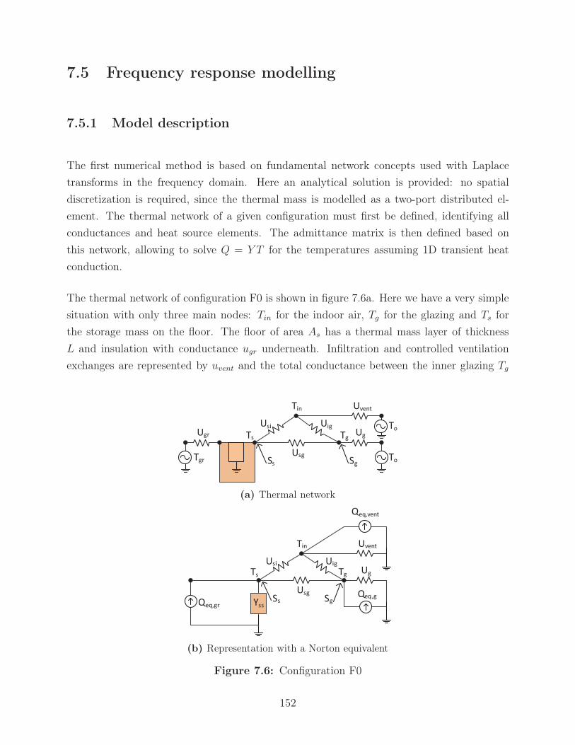
7.5 Frequency response modelling

7.5.1 Model description

The first numerical method is based on fundamental network concepts used with Laplace

transforms in the frequency domain. Here an analytical solution is provided: no spatial

discretization is required, since the thermal mass is modelled as a two-port distributed el-

ement. The thermal network of a given configuration must first be defined, identifying all

conductances and heat source elements. The admittance matrix is then defined based on

this network, allowing to solve Q = Y T for the temperatures assuming 1D transient heat

conduction.

The thermal network of configuration F0 is shown in figure 7.6a. Here we have a very simple

situation with only three main nodes: Tin for the indoor air, Tg for the glazing and Ts for

the storage mass on the floor. The floor of area As has a thermal mass layer of thickness

L and insulation with conductance ugr underneath. Infiltration and controlled ventilation

exchanges are represented by uvent and the total conductance between the inner glazing Tg

���

���

���

���

��� ���

��

��

���

�� ��

�� ��

��

(a) Thermal network

������

��

��

��

���

��� ���

��

���

������

��

�����

�����

(b) Representation with a Norton equivalent

Figure 7.6: Configuration F0

152

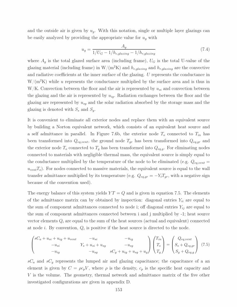
and the outside air is given by ug. With this notation, single or multiple layer glazings can

be easily analyzed by providing the appropriate value for ug with

ug =Ag

1/UG − 1/hc,glazing − 1/hr,glazing

(7.4)

where Ag is the total glazed surface area (including frame), UG is the total U-value of the

glazing material (including frame) in W/(m2K) and hc,glazing and hr,glazing are the convective

and radiative coefficients at the inner surface of the glazing. U represents the conductance in

W/(m2K) while u represents the conductance multiplied by the surface area and is thus in

W/K. Convection between the floor and the air is represented by usi and convection between

the glazing and the air is represented by uig. Radiation exchanges between the floor and the

glazing are represented by usg and the solar radiation absorbed by the storage mass and the

glazing is denoted with Ss and Sg.

It is convenient to eliminate all exterior nodes and replace them with an equivalent source

by building a Norton equivalent network, which consists of an equivalent heat source and

a self admittance in parallel. In Figure 7.6b, the exterior node To connected to Tin has

been transformed into Qeq,vent, the ground node Tgr has been transformed into Qeq,gr and

the exterior node To connected to Tg has been transformed into Qeq,g. For eliminating nodes

connected to materials with negligible thermal mass, the equivalent source is simply equal to

the conductance multiplied by the temperature of the node to be eliminated (e.g. Qeq,vent =

uventTo). For nodes connected to massive materials, the equivalent source is equal to the wall

transfer admittance multiplied by its temperature (e.g. Qeq,gr = −YtTgr, with a negative sign

because of the convention used).

The energy balance of this system yields Y T = Q and is given in equation 7.5. The elements

of the admittance matrix can by obtained by inspection: diagonal entries Yii are equal to

the sum of component admittances connected to node i; off diagonal entries Yij are equal to

the sum of component admittances connected between i and j multiplied by -1; heat source

vector elements Qi are equal to the sum of the heat sources (actual and equivalent) connected

at node i. By convention, Qi is positive if the heat source is directed to the node.

⎛⎜⎝

sCa + usi + uig + uvent −usi −uig

−usi Ys + usi + usg −usg

−uig −usg sCg + uig + usg + ug

⎞⎟⎠

⎛⎜⎝

Tin

Ts

Tg

⎞⎟⎠ =

⎛⎜⎝

Qeq,vent

Ss + Qeq,gr

Sg + Qeq,g

⎞⎟⎠ (7.5)

sCa and sCg represents the lumped air and glazing capacitance; the capacitance of a an

element is given by C = ρcpV , where ρ is the density, cp is the specific heat capacity and

V is the volume. The geometry, thermal network and admittance matrix of the five other

investigated configurations are given in appendix D.

153

The self and transfer admittances are complex numbers used to represent the response of a

system to a specific frequency (in the form of a predetermined design period). They can be

obtained by performing a Laplace transform on the 1D heat conduction equation

∂2T

∂x2=

1

α

∂T

∂t(7.6)

and elaborating a Norton equivalent network. A cascade matrix for a multilayer wall can be

defined by specifying boundary conditions adequate for a two-port model. For a structure

with two layers (i.e. mass + insulation with negligible capacitance), the cascade matrix is

given by ⎛⎜⎜⎝T1

Q1

⎞⎟⎟⎠ =

⎛⎜⎜⎝ cosh(γnL)

cosh(γnL)ugr

+sinh(γnL)

kγn

kγ sinh(γnL)kγn sinh(γnL)

ugr+ cosh(γnL)

⎞⎟⎟⎠

⎛⎜⎜⎝ T2

−Q2

⎞⎟⎟⎠ (7.7)

The self and transfer admittance have been definer earlier in equation 7.1 and 7.9. From

these definitions and the cascade matrix given above, the self and transfer admittance char-

acterizing the floor in configuration F0 are given by

Ys =As (Ugr + kγn tanh(γnL))

Ugr

kγntanh(γnL) + 1

(7.8)

Yt =−As

1

Ugr

cosh(γnL) +1

kγn

sinh(γnL)(7.9)

where k is the storage mass thermal conductivity, γn is equal to (s/αth)1/2 with s being the

Laplace transform variable and αth the storage mass thermal diffusivity. For the frequency

domain analysis conducted here, s is equal to ωj where ω is the frequency and j =√−1.

Additional details about the procedure for elaborating the Norton equivalent network and

deriving the cascade matrix for multilayered walls can be obtained in Athienitis et al. (1986)

and in Athienitis and O’Brien (2015).

Since the solution is obtained in the frequency domain, all elements composing the admittance

matrix must remain constant in time, including the radiative and convective coefficients.

Since the convective and radiative coefficients of a surface depend on its temperature, they

are determined in two iterations; estimated initial values are first provided and detailed

coefficients are calculated at the second iteration based on the average temperature of the

surfaces obtained from the first iteration. The convective coefficients are calculated using

Khalifa and Marshall (1990) correlations. Since all glazed surfaces are grouped together,

154

the convective coefficient of the tilted glazed roof is the same as for a vertical glazing. The

radiative coefficient between two surfaces is calculated with (Duffie and Beckman, 2006,

eq. 3.10.2)

hr,ij =4σT 3

m

1 − εi

εi+

1

Fij+

(1 − εj)Ai

εjAj

(7.10)

where σ is the Stefan-Boltzmann constant, Tm is the mean temperature of surfaces i and j

over the investigated time sequence, ε represents the emissivity and Fij is the view factor.

Equations for the calculation of view factors can be found in Appendix C.3.

Elements composing the heat source vector must provide steady periodic conditions; there-

fore, the analysis with this model is focused on short design sequences. The temperature and

solar radiation profiles of a specially chosen design period have to be defined for a specific

location. The importance of the design sequence selection in discussed in section 7.5.2.5.

The temperature profile is based on a sinusoidal function with a maximum at 3pm. The aver-

age temperature is taken as the monthly average temperature for the month under consider-

ation. The amplitude of the temperature profile is taken as the average monthly temperature

variations divided by two.

The solar radiation incident on a surface for a sunny design day is computed using the Hottel

clear sky method (Hottel, 1976) for the design day under consideration. A cloudy design day

was constructed by setting the beam solar radiation to zero and multiplying the diffuse solar

radiation by 1.5 from the Hottel model, which is representative of a completely overcast day.

The solar radiation transmitted through the glazings of different orientations and absorbed by

the interior surfaces is calculated separately with another routine that combines ray tracing

and radiosity techniques. Detailed calculations are presented in Bastien et al. (2015).

Once the temperature profile and the solar radiation absorbed by the interior surfaces have

been determined, complex Fourier series are required in order to calculate the time domain

solution for these vectors. Five harmonics were selected for a 24 h design period. As reported

in Athienitis et al. (1986), the magnitude of the self admittance Ysn increases with the har-

monic number while the penetration depth (αth/ω)1/2 decreases. This is further exemplified

by the shift in the peak Ysn magnitude, which occurs at a smaller thickness as the harmonic

number increases (results not shown). However, by studying the effect of harmonics num-

ber on the storage temperature swings, Athienitis et al. (1986) reported that three to five

harmonics are sufficient to ensure that the accuracy of the swings is about 0.1 °C.

155

Simulations with the FR model are executed with a time step of 0.05 h. A time step of 0.5 h

would have been satisfying, but a smaller time step was selected in order to have a better

resolution for the analysis of τ[Qa−Ts]. Simulation results obtained with the FR model are

presented in section 7.5.2 below. Unless indicated otherwise, simulations in this section are

conducted for configuration N1 with dimensions of h=3 m, w=2.4 m, l=10 m equipped with

a clear double insulated glazed unit with a concrete TES and no active air circulation for a

periodic sunny day at the winter solstice for a latitude of 45°. The impacts resulting from

varying these characteristics will be analyzed in the following subsections.

The analysis is focused on the main performance variables identified in section 7.3.7. In the

following discussion, the word optimal refers to the extremum of one of these variables.

7.5.2 Simulation results and discussion

7.5.2.1 Main results – all configurations

As shown on figure 7.7a, under the conditions described above, the minimum operative

temperature becomes fairly stable for thicknesses beyond 0.20 m for all configurations. It is

significantly affected by the solarium design, and positioning the mass on the wall instead of

the floor (F1→N1) raises the minimum temperature by almost 2 °C.

The observation of figure 7.7b reveals that the maximum operative temperature is also

strongly affected by the design. The maximum temperature becomes relatively stable for

thicknesses beyond 0.10 m for all configurations. The same observations also apply to the

average temperature swing (see figure 7.7c).

The effect of the solarium design on the average temperature is very significant: having an

opaque north wall instead of being glazed raises the average temperature by about 12 °C

(F0→ F1). For the same thickness of thermal mass, locating the mass on the north wall

instead of the floor will results in slightly higher average temperature (F1→N1).

As explained in section 7.3.1, τ[Qa−Ts] is the time lag between the peak absorbed solar radi-

ation heat flux and the peak storage temperature. We can see in figure 7.7e that increasing

the solar radiation collection of the space (by changing the north wall from being glazed

to opaque, i.e. F0→F1), can increase τ[Qa−Ts] by about 0.4 h. It peaks at 5-8 cm for all

configurations, and becomes fairly constant for thicknesses greater than 22 cm.

156

Thickness (m)

Tem

per

atur

e(°

C)

Minimum operative temperature

F0F1N1N2

0.01 0.05 0.1 0.15 0.2 0.25 0.3 0.35 0.4-10

-8

-6

-4

-2

0

2

4

6

8

10

(a)

Thickness (m)

Tem

per

atur

e(°

C)

Maximum operative temperature

F0F1N1N2

0.01 0.05 0.1 0.15 0.2 0.25 0.3 0.35 0.410

20

30

40

50

60

70

80

(b)

Thickness (m)

Tem

per

atur

e(°

C)

Average operative temperature swing

F0F1N1N2

0.01 0.05 0.1 0.15 0.2 0.25 0.3 0.35 0.410

20

30

40

50

60

70

80

90

(c)

Thickness (m)

Tem

per

atur

e(°

C)

Average operative temperature

F0F1N1N2

0.01 0.05 0.1 0.15 0.2 0.25 0.3 0.35 0.42

4

6

8

10

12

14

16

18

20

(d)

Thickness (m)

Pha

sesh

ift

(h)

Solar radiation - storage temperature time lag

F0F1N1N2

0.01 0.05 0.1 0.15 0.2 0.25 0.3 0.35 0.4

1.4

1.6

1.8

2

2.2

2.4

2.6

2.8

3

(e)

Figure 7.7: Main output performance variables – configurations F0, F1, N1 and N2

157

34

5

5

5

6

6 6 6

7

7

7 7 7

8

8

8 8 8

9

9

99

Floor thickness (m)

Wal

lth

ickn

ess

(m)

0.05 0.1 0.2 0.3 0.40.05

0.1

0.2

0.3

0.4

(a) Minimum operative temperature (°C)

26

26

26

26

2627

27

27 27 27

2828

28

28 28 282929 29

30 30 3031

Floor thickness (m)

Wal

lth

ickn

ess

(m)

0.05 0.1 0.2 0.3 0.40.05

0.1

0.2

0.3

0.4

(b) Maximum operative temperature (°C)

1818

18 18 18

20

20

20 20 20

22

22

22 22 2224

24 242628

Floor thickness (m)

Wal

lth

ickn

ess

(m)

0.05 0.1 0.2 0.3 0.40.05

0.1

0.2

0.3

0.4

(c) Average operative temperature swing (°C)

15.162

15.1

64

15.164 15.164

15.1

66

15.16615.166 15.166

15.1

68

15.168

15.168

15.168

15.16815.168 15.168

15.17

15.1715

.17

Floor thickness (m)

Wal

lth

ickn

ess

(m)

0.05 0.1 0.2 0.3 0.40.05

0.1

0.2

0.3

0.4

(d) Average operative temperature (°C)

1.8

1.8

1.8 1.8 1.822 2 2

2.2 2.2 2.22.4 2.4 2.42.6 2.6 2.62.8

Floor thickness (m)

Wal

lth

ickn

ess

(m)

0.05 0.1 0.2 0.3 0.40.05

0.1

0.2

0.3

0.4

(e) Wall τ[Qa−Ts] (h)

1.8

1.8

1.8 1.8

22

2

2 2

2.22.2

2.2 2.2

2.42.4

2.4

2.62.6

2.6

2.8

33.2

Floor thickness (m)

Wal

lth

ickn

ess

(m)

0.05 0.1 0.2 0.3 0.40.05

0.1

0.2

0.3

0.4

(f) Floor τ[Qa−Ts] (h)

Figure 7.8: Main output performance variables – configuration FN1

158

678

8 8 8

9

9 9 9

10

10

10 10 10

11

11

11 11

Floor thickness (m)

Wal

lth

ickn

ess

(m)

0.05 0.1 0.2 0.3 0.40.05

0.1

0.2

0.3

0.4

(a) Minimum operative temperature (°C)

3030

30

3031

31

31 31 31

3232

32

32 32 32

33

33 33 3334 34 34

Floor thickness (m)

Wal

lth

ickn

ess

(m)

0.05 0.1 0.2 0.3 0.40.05

0.1

0.2

0.3

0.4

(b) Maximum operative temperature (°C)

2020

20 20 20

22

22

22 22 22

24

24 24 2426 26 2628

Floor thickness (m)

Wal

lth

ickn

ess

(m)

0.05 0.1 0.2 0.3 0.40.05

0.1

0.2

0.3

0.4

(c) Average operative temperature swing (°C)

18.3

2

18.32 18.32

18.3

22

18.322 18.322 18.322

18.322

18.3

24

18.324

18.32418.324

18.32418.324 18.324

18.326

18.326

18.326

Floor thickness (m)

Wal

lth

ickn

ess

(m)

0.05 0.1 0.2 0.3 0.40.05

0.1

0.2

0.3

0.4

(d) Average operative temperature (°C)

1.61.6

1.6

1.61.6

1.6

1.8

1.8 1.8 1.822 2 2

2.2 2.2 2.22.4 2.4 2.42.6 2.6 2.62.8

Floor thickness (m)

Wal

lth

ickn

ess

(m)

0.05 0.1 0.2 0.3 0.40.05

0.1

0.2

0.3

0.4

(e) Wall τ[Qa−Ts] (h)

1.8

1.8

1.8 1.8

22

2

22

2.22.2

2.2

2.2 2.2

2.42.4

2.4

2.62.6

2.6

2.8

33.2

Floor thickness (m)

Wal

lth

ickn

ess

(m)

0.05 0.1 0.2 0.3 0.40.05

0.1

0.2

0.3

0.4

(f) Floor τ[Qa−Ts] (h)

Figure 7.9: Main output performance variables – configuration FN2

159

Simulation results for configurations FN1 and FN2 are shown in figures 7.8-7.9. We can see

from figure 7.8a that the highest minimum operative temperature is 9.2 °C and occurs for a

thickness of 0.27 m for both the floor and wall storage; it remains above 9.0 °C as long as

both TES are at least 0.2 m or larger. As seen on figure 7.8c, the minimum swing is 17 °C

and occurs at a thickness of 0.18 m for both TES. It remains below 18°C as long as both

TES have a minimum thickness of 0.12 m.

For FN1, the maximum wall τ[Qa−Ts] is 2.8 h and occurs when both TES are 5-6 cm thick.

It is greater than 2.5 h when both TES are equal or less than 10 cm. The floor τ[Qa−Ts] is

maximum at 3.3 h for a 5 cm wall and a 6-8 cm floor and is above 2.8 h when both TES are

between 5 and 9 cm. Therefore, implementing a 6 cm storage on both the wall and the floor

maximizes τ[Qa−Ts] for both TES.

Having storage on both the wall and the floor instead of just the wall (N1→FN1) can increase

the highest minimum operative temperature by up to 7 °C. As seen in figure 7.9a, the highest

minimum operative temperature is 11.8 °C and occurs for a thickness of 0.24-0.29 m for both

TES. It remains above 11.6 °C as long as at both TES are at least 0.20 m. Having opaque

east and west walls (FN1→FN2) does not significantly impact τ[Qa−Ts] for both TES.

7.5.2.2 Impact of varying floor area dimensions, aspect ratio and orientation

Although a detailed study of design parameters and their influence on the indoor climate is

beyond the scope of this work, simulation results for configurations F0 and N1 with varying

dimensions are presented below. The investigated dimensions are given in table 7.3.

Table 7.3: Simulated floor area dimensions and aspect ratio

Configuration North wall Width (m) Length (m)

height (m)

F0-s 3 2.4 10

F0-m 4 4 10

F0-l 4 4 100

N1-s 3 2.4 4

N1-m 4 4 4

N1-l 3 2.4 10

As seen in figure 7.10, we can see that varying the floor area and aspect ratio of configurations

F0 and N1 has little impact on the optimal thermal storage thickness of the main performance

parameters. Varying the floor area of a fully glazed greenhouse (F0) has virtually no impact

160

Thickness (m)

Tem

per

atur

e(°

C)

Top avDaily av Top swing

0.01 0.05 0.1 0.15 0.2 0.25 0.3 0.35 0.40

5

10

15

20

25

30

35

40

(a) Average Top and its swing, F0

Thickness (m)

Tem

per

atur

e(°

C)

Top avDaily av Top swing

0.01 0.05 0.1 0.15 0.2 0.25 0.3 0.35 0.40

10

20

30

40

50

60

(b) Average Top and its swing, N1

Thickness (m)

Tem

per

atur

e(°

C)

Top minTop max

0.01 0.05 0.1 0.15 0.2 0.25 0.3 0.35 0.4-10

-5

0

5

10

15

20

25

30

35

40

(c) Minimum and maximum Top, F0

Thickness (m)

Tem

per

atur

e(°

C)

Top minTop max

0.01 0.05 0.1 0.15 0.2 0.25 0.3 0.35 0.4-10

0

10

20

30

40

50

(d) Minimum and maximum Top, N1

Figure 7.10: Impact of varying floor area; small, medium, large

of the main performance parameters. Changes in the floor area and aspect ratio for a solarium

with a massive north wall (N1) can have a small impact. From figure 7.10b, we can see that

a solarium design aligned on a east-west axis with a higher aspect ratio experiences a higher

average temperature, which is coherent with many studies that identified that it was most

beneficial for greenhouses to have their longest side facing south (Harnett, 1975; Kozai, 1977b;

Rosa et al., 1989; Gupta and Chandra, 2002). The solar radiation - storage temperature time

lag is identical for the F0-s, -m and -l while it converges to a slightly higher value (0.1-0.2 h)

for the N1 design with higher aspect ratios; changing the orientation from due south reduces

the absorbed solar radiation, and thus lower the average and peak operative temperatures

and its swing (results not shown). It can be seen that even though the main performance

parameters can be affected by variations in the floor area and aspect ratio, their response to

varying thermal storage thickness is similar.

161

7.5.2.3 Impact of TES material

In this work, the reference thermal storage material is concrete as it is a widely used material

that has been studied extensively, thus facilitating comparison with the existing literature.

In addition, concrete is often present in buildings for structural reasons; therefore keeping it

exposed and available for thermal storage could improve indoor climate with no additional

cost. However, for thicknesses greater than 0.2-0.3 m, the cost and environmental impacts of

this material are likely to hinder its use in bigger volumes, making the study of inexpensive

and readily available materials a necessity for large TES. This section presents a comparison

of the performance of concrete TES with soil and water TES.

The thermal properties of soil are highly dependent on the soil type (i.e. the proportion of

sand, silt and clay) and moisture content. In particular, changes in its thermal conductivity

can significantly alter heat transfer exchanges; typical values are between 0.6-2.5 W/m2-K,

depending on the soil type and moisture content (ASHRAE, 2009, F25). Because of the

variability of soil properties, two different types of soil are analyzed here: a sandy loam

soil and clay loam soil. Properties representative of these two types of soil are indicated in

table 7.4.

Table 7.4: TES materials properties

k cp ρ

Concrete 1.73 W/m2-K 840 J/kg-K 2243 kg/m3

Soil - sandy loam 0.8 W/m2-K 800 J/kg-K 1600 kg/m3

Soil - clay loam 1.2 W/m2-K 900 J/kg-K 1700 kg/m3

Water 0.59 W/m2-K 4813 J/kg-K 998.3 kg/m3

In the case of liquid TES such as water, convective heat transfer is present in addition to

conduction. As in the case of solid TES, it is assumed here that the water temperature is

uniform in a control volume. The conductivity of water is replaced by an effective conductivity

ke = Nu k where Nu is given by (Wright, 1996)

Nu = 0.0674Ra1/3 (7.11)

For a fluid contained in a rectangular unit of width L with a temperature difference ΔT, the

Rayleigh number is calculated with

Ra =gβthΔTL3

ναth(7.12)

162

where βth is the thermal expansion coefficient, ν is the kinematic viscosity and αth is the

thermal diffusivity of water. Here the effective conductivity is calculated at every thickness

for a nominal temperature difference of 1 °C. Since the effective conductivity is proportional

to ΔT 1/3, changes is ke are much smaller then changes in ΔT ; therefore the impacts of this

simplification are not very significant.

As seen from figure 7.11a, a TES made of water experiences the smallest temperature swings

from the four materials investigated. In addition, a clay loam soil is significantly more efficient

than a sandy loam soil for reducing temperature swings. The average temperature is very

similar for these four materials.

Thickness (m)

Tem

per

atur

e(°

C)

Top avDaily av Top swing

0.01 0.1 0.2 0.3 0.4 0.5 0.6 0.7 0.8 0.9 110

15

20

25

30

35

40

45

50

55

60

(a) Average Top and it’s swing

Thickness (m)

Tem

per

atur

e(°

C)

Top minTop max

0.01 0.1 0.2 0.3 0.4 0.5 0.6 0.7 0.8 0.9 1-10

0

10

20

30

40

50

60

(b) Minimum and maximum Top

Thickness (m)

Tim

ela

g(h

)

concretesandy loamclay loamwater

0.01 0.1 0.2 0.3 0.4 0.5 0.6 0.7 0.8 0.9 11.4

1.6

1.8

2

2.2

2.4

2.6

2.8

3

3.2

3.4

(c) τ[Qa−Ts]

Figure 7.11: Impact varying of storage material; sandy loam, concrete, clayloam, water

163

A TES made of water experiences reduced peak temperatures, followed by concrete and clay

loam soil (see figure 7.11b). As shown on figure 7.11c, all investigated materials except water

reach a constant time lag at 0.20 m and beyond. Water has s significantly wider and higher

peak, with a peak time lag decreasing much more slowly than for the other materials.

7.5.2.4 Impact of varying thermal resistance of the insulation layer

So far, all simulations have been conducted with an insulation layer having a thermal re-

sistance of RSI 20 (R 114). Such a high value was chosen with the objective of providing

near adiabatic conditions at the outside storage mass layer to focus our attention on the heat

absorbed and released at the inside layer.

It is well known that increased thermal resistance reduces heat fluxes with diminishing re-

turns. Exactly how much insulation should be selected depends on economic, space and

performance constraints. The sensitivity of the five main performance variables to varying

insulation levels was assessed for RSI 2, 5 and 20 insulation levels. The biggest impact was

observed for the minimum and average operative temperature. The average temperature was

1.0 °C lower for all thicknesses with RSI 2 compared to RSI 20 and the minimum temperature

dropped by 1.0 °C for thicknesses between 0.2-1 m. Variations of the maximum operative

temperature and it’s swing were not significant and are therefore not presented.

The transfer admittance as a function of storage thickness is shown in figure 7.12b for the

three different insulation levels. We can see that the transfer admittance approaches zero at

storage thicknesses of 0.4 m and beyond for the three investigated insulation levels.

Thickness (m)

Tem

per

atur

e(°

C)

Top minTop av

0.01 0.1 0.2 0.3 0.4 0.5 0.6 0.7 0.8 0.9 1-10

-5

0

5

10

15

20

(a) Minimum and average operative temperature

Thickness (m)

Tra

nsfe

rad

mit

tanc

em

agni

tude

(W/°

C)

RSI 2RSI 5RSI 20

0.01 0.1 0.2 0.3 0.4 0.5 0.6 0.7 0.8 0.9 10

5

10

15

(b) Magnitude of the transfer admittance

Figure 7.12: Impact of varying thermal resistance of the insulation layer; RSI 5,RSI 10, RSI 20

164

Analyzing the transfer admittance in isolation could induce to conclude that there is no

benefits to increase the insulation layer from RSI 2 to 5 or 20 for storage thicknesses beyond

0.4 m, but the observation of the minimum and average temperature reveals that the penalty

for reduced insulation level is fairly constant for thicknesses between 0.1 and 1 m.

Although informative, it is not possible to extract definitive conclusions from the simulation

results presented above. Therefore, the impact of varying the thermal resistance of the

insulation layer will be investigated with the FD model under real weather conditions in the

next section.

7.5.2.5 Impact of design sequence selection

Figure 7.13 shows the simulation results over different periodic design sequences ranging

from a sunny day to seven sunny days followed by seven cloudy days. It can be seen that the

optimal thickness in regards to the minimum, maximum and average operative temperatures

is significantly affected by the choice of the design period.

As shown in figure 7.13a, the minimum temperature peak occurs at larger thicknesses with

increasing consecutive cloudy days. Under a 7 sunny - 7 cloudy days design period, the

minimum temperature for a TES thickness of 0.10 m is -5.4 °C while it reaches a minimum

of -2.5 °C at 1.18 m. This is an important result that can justify the use of larger TES for

applications where raising the minimum temperature is an important concern.

The maximum operative temperature exhibits a different behavior (see figure 7.13b). Under

a sunny day and a 1 sunny - 1 cloudy days design periods, the extremum occurs between 0.13-

0.15 m, while it occurs at thicknesses greater than 0.49 m for sequences with two consecutive

cloudy days or more. As the number of consecutive cloudy days increases, two minima become

visible: one around 0.10-0.15 m and a lower minima at a significantly greater thickness.

Figure 7.13c illustrates the swing of the daily average operative temperature for different

design day periods. It can be seen that it is mainly independent of the design period. The

minimum swing occurs between 0.17 and 0.23 m and then converges to a constant value

at 0.40 m and beyond. The swing is 0.04-0.41 °C lower at the minima than the value for

thicknesses greater than 0.40 m. At small thicknesses (<0.10 m), the temperature swing is

very sensitive to the TES thickness.

As seen from figure 7.13d, the maximum average temperature occurs at a greater thickness

when the number of consecutive cloudy days increases, but the overall magnitude of the

variations in average temperature with thickness is very small.

165

Thickness (m)

Tem

per

atur

e,(°

C)

1Sunny1Sunny-1Cloudy2Sunny-2Cloudy3Sunny-3Cloudy5Sunny-5Cloudy7Sunny-7Cloudy

0.01 0.1 0.2 0.3 0.4 0.5 0.6 0.7 0.8 0.9 1 1.1 1.2-10

-8

-6

-4

-2

0

2

4

6

(a) Minimum operative temperature

Thickness (m)

Tem

per

atur

e(°

C)

1Sunny1Sunny-1Cloudy2Sunny-2Cloudy3Sunny-3Cloudy5Sunny-5Cloudy7Sunny-7Cloudy

0.01 0.1 0.2 0.3 0.4 0.5 0.6 0.7 0.8 0.9 1 1.1 1.228

30

32

34

36

38

40

42

44

46

48

(b) Maximum operative temperature

Thickness (m)

Tem

per

atur

e(°

C)

y

1Sunny-1Cloudy2Sunny-2Cloudy3Sunny-3Cloudy5Sunny-5Cloudy7Sunny-7Cloudy

0.01 0.1 0.2 0.3 0.4 0.5 0.6 0.7 0.8 0.9 1 1.1 1.219

20

21

22

23

24

25

(c) Daily average operative temperature swing

Thickness (m)

Tem

per

atur

e(°

C)

1Sunny-1Cloudy2Sunny-2Cloudy3Sunny-3Cloudy5Sunny-5Cloudy7Sunny-7Cloudy

0.01 0.1 0.2 0.3 0.4 0.5 0.6 0.7 0.8 0.9 1 1.1 1.27.04

7.06

7.08

7.1

7.12

7.14

7.16

7.18

7.2

(d) Average operative temperature

Thickness (m)

Tem

per

atur

e(°

C)

SunnyCloudy

0.01 0.05 0.1 0.15 0.2 0.25 0.3 0.35 0.4 0.45 0.51.6

1.8

2

2.2

2.4

2.6

2.8

3

3.2

3.4

3.6

(e) τ[Qa−Ts]

Thickness (m)

Pha

sesh

ift

(h)

summer solsticeequinoxwinter solstice

0.01 0.05 0.1 0.15 0.2 0.25 0.3 0.35 0.4 0.45 0.5

1.4

1.6

1.8

2

2.2

2.4

2.6

2.8

3

3.2

(f) τ[Qa−Ts]

Figure 7.13: Impact of design sequence selection – configuration N1

166

The impacts of solar radiation availability on τ[Qa−Ts] are shown in Figure 7.13e, where results

for a sunny day and a cloudy day at the winter solstice are compared. Although the τ[Qa−Ts]

is higher for a cloudy day, its peak occurs at the same thickness whether the design period

is a cloudy day or a sunny day.

Figure 7.13f shows τ[Qa−Ts] for three different moment in the year. Here simulations were

conducted under the periodic conditions of a sunny day at the winter solstice, the vernal

equinox and the summer solstice. Since a solarium design cannot be optimized simultaneously

for different time of the year, a designer should carefully select a day representative of the

moment of the year when the time lag is most desirable. However, the choice of a specific day

is not of crucial importance since the behavior of τ[Qa−Ts] does not exhibit very significant

variations throughout the year. It can be seen that τ[Qa−Ts] is maximum at 5-7 cm at the

winter solstice while it peaks at 6-8 cm at the equinox and 7-9 cm at the summer solstice.

One could choose to optimize the time lag at the winter solstice, because then solar gains are

at their lowest levels and therefore more needed.

7.5.2.6 Discussion

The impacts of varying glazing type and enhanced thermal coupling have been analyzed

and simulations results are presented in appendix E. It is observed that the introduction

of continuous indoor air recirculation increases convective exchanges and can significantly

reduces the maximum operative temperature, but reduces slightly its average and minimum

temperature as well as τ[Qa−Ts]. In addition, the glazing type significantly affect the average

operative temperature and its peaks, but not much the optimal TES thickness.

As we can see from the results presented so far, under periodic design sequences, there seems

to be three different optimal TES thicknesses for fulfilling different objectives: the optimal

thickness for reducing daily average temperature swings is between 0.15-0.25 m, the optimal

thickness for maximizing τ[Qa−Ts] is around 0.05-0.10 m while reducing operative temperature

peaks needs a greater thickness as the number of consecutive cloudy days increases. How-

ever, the magnitude of improvement of these three performance variables is relatively small;

investigating how these will translate under real weather conditions is important and will be

studied in the next section.

Although frequency response modelling can be used to analyze any periodic conditions, and

it is possible to create period conditions from non-periodic ones by increasing the simulation

period and repeating the conditions, this modelling method is more appropriate for short

167

term analysis using design sequences. For accurate simulations, more harmonics are needed

as the design period increases, which significantly impacts simulation time. For instance,

for a one-day design period, 5 harmonics were sufficient, while 43 harmonics were necessary

to analyze a 7 sunny - 7 cloudy days design period; this increased the computational time

by a factor of 140. The use of a finite difference (FD) model is more appropriate for yearly

simulations with real weather data.

7.6 Finite difference modelling

Here the previously developed frequency response (FR) model will be compared with a model

using the finite difference (FD) method. The FR model will be progressively modified towards

a finite difference thermal network model that will consider non linear radiative and convective

heat transfer. The major modeling steps are presented in the first subsection where their

impacts on accuracy and computational efficiency are discussed. The second subsection

presents results obtained with the FD model.

7.6.1 Model parameters

All simulation results presented in this section are for configuration F0 subjected to a sunny

day at the winter solstice unless specified otherwise.

7.6.1.1 Spatial discretization

The first modification introduced is the spatial discretization of the thermal mass. First, the

accuracy of two different discretization schemes is analyzed. With the "3Ne" model, half of

the mass is located at the center and one quarter at the edges (see Figure 7.14). With the

"3Nc" model, 1/4 of the mass is in the center and 3/8 of the mass is located at 1/4 of the

total thickness.

Figure 7.15a depicts the average temperature swings obtained with the FR model with dis-

tributed mass and with the "3Ne" and "3Nc" discretization schemes. It can be seen that

models with thermal mass at the edges are more accurate and therefore adopted.

Figure 7.15b shows the impact of increasing the number of control volumes from three to

seven. Spatial discretization with three control volumes shows good adequacy until a thick-

168

Figure 7.14: Two spatial discretization schemes

ness of about 0.2 m, but then diverges from the FR model, with the difference getting bigger

with increasing thickness. As can be seen, a greater number of control volumes is needed to

maintain accuracy as the thickness increases.

Thickness (m)

Tem

per

atur

esw

ing,

°C

FRFR 3NeFR 3Nc

0.1 0.2 0.3 0.4 0.5 0.6 0.7 0.8 0.9 15

10

15

20

25

30

(a) Impact of spatial discretization scheme

Thickness (m)

Tem

per

atur

esw

ing,

°C

FRFR 3NFR 5NFR 7N

0.1 0.2 0.3 0.4 0.5 0.6 0.7 0.8 0.9 16

8

10

12

14

16

18

20

(b) Impact of increasing control volumes

Figure 7.15: Temperature swing as a function of TES thickness; Ts, Top

Here TES with thicknesses between 0.1 and 1 m are analyzed. Analyzing smaller thicknesses

would necessitate a very small time step (see next section); thus the limit was set at 0.1 m.

Although TES as thick as 5.5 m have been built (as seen in the literature review), 1 m is

deemed sufficient to evaluate potential benefits of large TES in solaria and greenhouses.

As seen from figure 7.16, for the aforementioned conditions and for thicknesses up to 1 m,

introducing a spatial discretization scheme with thermal mass at the edges and lumping

the capacitance in 23 control volumes provides a good adequacy with the FR model with

distributed mass. Therefore these parameters are adopted.

169

Thickness (m)

Tem

per

atur

esw

ing,

°C

FR

FR 11N

0.1 0.2 0.3 0.4 0.5 0.6 0.7 0.8 0.9 114

15

16

17

18

19

20

(a) 11N

Thickness (m)

Tem

per

atur

esw

ing,

°C

FR

FR 23N

0.1 0.2 0.3 0.4 0.5 0.6 0.7 0.8 0.9 114

15

16

17

18

19

20

(b) 23N

Figure 7.16: Operative temperature swing as a function of TES thickness; Ts, Top,+ indicates extremum, � indicates extremum ±0.15 and ♦ indicates extremum ±0.3

7.6.1.2 Temporal discretization

Developing a lumped parameter FD model requires introducing temporal discretization. The

basic Euler forward method is adopted, which has a fully explicit scheme:

Ti,t+1 =Δt

C

(Qi,t+hc,iAi(Tair,t−Ti,t)+

∑j

(Tj,t−Ti,t)R−1ij +Ai

∑k

hr,ik(Tk,t−Ti,t)

)+Ti,t (7.13)

where C is the capacitance of node i, Qi,t is a heat source at node i, Rij is the thermal resis-

tance between nodes i and j (in K/W), j represents nodes experiencing conductive exchanges

with i, k represents nodes experiencing radiative exchanges with i and other symbols were

previously defined. For comparison purposes, the convective and radiative coefficients, initial

conditions and solar radiation and temperature profiles are retrieved from the FR model and

used as input for the FD model in this subsection.

The Euler forward discretization scheme was adopted since it is easy to implement and

computationally fast. Given the large number of control volumes required for accuracy, a

time step of 0.002 h (7.2 s) is used to guarantee stability. Even with such a small time step,

annual simulations can be carried out at a reasonable speed (about 40 minutes). The hourly

weather data input are not interpolated to fit this time step.

The temperature swings obtained with the FR model, the FR model with discretized mass

and the FD model are depicted in figure 7.17 for comparison. It can be seen for the FD

170

Thickness (m)

Tem

per

atur

esw

ing,

°C

FRFR 23NFD 23N

0.1 0.2 0.3 0.4 0.5 0.6 0.7 0.8 0.9 114

15

16

17

18

19

20

Figure 7.17: Impact of temporal discretization; Ts, Top

model, a small discrepancy is introduced at a thickness of 0.4 m and beyond. Reducing

the time step below 0.002 h does not reduce the discrepancy. The maximum difference of

0.13 °C between the FR and the FD 23N models is considered acceptable for the scope of

this study.

7.6.1.3 Sensivity to radiative and convective coefficients

With the FR model, all parameters of the admittance matrix had to be kept constant during

the simulation period, including the radiative and convective coefficients. With this model,

the interior long wave radiation exchanges were calculated with a constant linearized radia-

tive heat transfer coefficient. Here these simulations are compared with the FD model using

the same linearized radiative coefficient but recalculated at every time step as a function

of the temperature of surfaces. A third model is also investigated with non linear radia-

tive coefficients calculated with the Gebhart method (Gebhart, 1959; Mottard and Fissore,

2007), where the net radiative flux emitted by a surface is calculated using the Gebhart

coefficients.

In this section, the configuration under study is F0, which is fully glazed. Consequently, the

radiative coefficient under study in this section is hr,floor−glazing.

The simulation results of these three radiation models are very close to each other where

only minimal variations can be observed in figure 7.18a. Mean and extreme values of the

radiative coefficient obtained with different calculation methods are presented in Table 7.5.

By observing Figure 7.18a, it can be seen that there is very little difference when using a

171

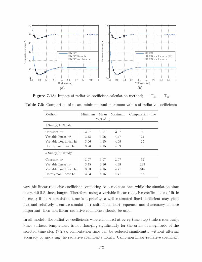
Thickness (m)

Tem

per

atur

esw

ing,

°C

FD 23NFD 23N linear hrFD 23N non linear hr

0.1 0.2 0.3 0.4 0.5 0.6 0.7 0.8 0.9 114

15

16

17

18

19

20

(a)

Thickness (m)

Tem

per

atur

esw

ing,

°C

FD 23NFD 23N non linear hr (1h)FD 23N non linear hr

0.1 0.2 0.3 0.4 0.5 0.6 0.7 0.8 0.9 114

15

16

17

18

19

20

(b)

Figure 7.18: Impact of radiative coefficient calculation method; Ts, Top

Table 7.5: Comparison of mean, minimum and maximum values of radiative coefficients

Method Minimum Mean Maximum Computation timeW/(m2K) s

1 Sunny/1 Cloudy

Constant hr 3.97 3.97 3.97 6Variable linear hr 3.78 3.96 4.47 24Variable non linear hr 3.96 4.15 4.69 25Hourly non linear hr 3.96 4.15 4.69 6

5 Sunny/5 Cloudy

Constant hr 3.97 3.97 3.97 52Variable linear hr 3.75 3.96 4.49 299Variable non linear hr 3.93 4.15 4.71 318Hourly non linear hr 3.93 4.15 4.71 56

variable linear radiative coefficient comparing to a constant one, while the simulation time

is are 4.0-5.8 times longer. Therefore, using a variable linear radiative coefficient is of little

interest; if short simulation time is a priority, a well estimated fixed coefficient may yield

fast and relatively accurate simulation results for a short sequence, and if accuracy is more

important, then non linear radiative coefficients should be used.

In all models, the radiative coefficients were calculated at every time step (unless constant).

Since surfaces temperature is not changing significantly for the order of magnitude of the

selected time step (7.2 s), computation time can be reduced significantly without altering

accuracy by updating the radiative coefficients hourly. Using non linear radiative coefficient

172

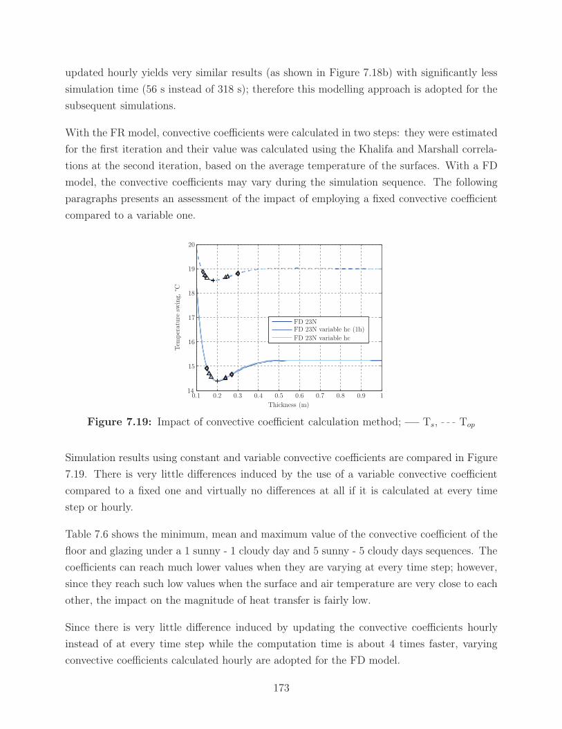
updated hourly yields very similar results (as shown in Figure 7.18b) with significantly less

simulation time (56 s instead of 318 s); therefore this modelling approach is adopted for the

subsequent simulations.

With the FR model, convective coefficients were calculated in two steps: they were estimated

for the first iteration and their value was calculated using the Khalifa and Marshall correla-

tions at the second iteration, based on the average temperature of the surfaces. With a FD

model, the convective coefficients may vary during the simulation sequence. The following

paragraphs presents an assessment of the impact of employing a fixed convective coefficient

compared to a variable one.

Thickness (m)

Tem

per

atur

esw

ing,

°C

FD 23NFD 23N variable hc (1h)FD 23N variable hc

0.1 0.2 0.3 0.4 0.5 0.6 0.7 0.8 0.9 114

15

16

17

18

19

20

Figure 7.19: Impact of convective coefficient calculation method; Ts, Top

Simulation results using constant and variable convective coefficients are compared in Figure

7.19. There is very little differences induced by the use of a variable convective coefficient

compared to a fixed one and virtually no differences at all if it is calculated at every time

step or hourly.

Table 7.6 shows the minimum, mean and maximum value of the convective coefficient of the

floor and glazing under a 1 sunny - 1 cloudy day and 5 sunny - 5 cloudy days sequences. The

coefficients can reach much lower values when they are varying at every time step; however,

since they reach such low values when the surface and air temperature are very close to each

other, the impact on the magnitude of heat transfer is fairly low.

Since there is very little difference induced by updating the convective coefficients hourly

instead of at every time step while the computation time is about 4 times faster, varying

convective coefficients calculated hourly are adopted for the FD model.

173

Table 7.6: Comparison of mean, minimum and maximum values of convective coefficients

Method Minimum Mean Maximum Computation time

W/(m2K) s

1 Sunny/1 Cloudy

Constant hcfloor 3.02 3.02 3.02 6

Variable hcfloor 0.41 2.94 3.33 25

Hourly hcfloor 1.77 2.95 3.33 6

Constant hcglazing 7.17 7.17 7.17 6

Variable hcglazing 4.48 7.13 7.42 25

Hourly hcglazing 6.41 7.15 7.42 6

5 Sunny/5 Cloudy

Constant hcfloor 3.01 3.01 3.01 52

Variable hcfloor 0.20 2.93 3.43 301

Hourly hcfloor 1.59 2.93 3.43 58

Constant hcglazing 7.17 7.17 7.17 52

Variable hcglazing 3.54 7.11 7.49 301

Hourly hcglazing 5.33 7.11 7.49 58

Thickness (m)

Tem

per

atur

esw

ing,

°C

FR

FD

0.1 0.2 0.3 0.4 0.5 0.6 0.7 0.8 0.9 114

15

16

17

18

19

20

Figure 7.20: Comparison of the FR and FD models, configuration F0; Ts, Top

Comparisons of the storage and operative temperature swings obtained with the FR and FD

models with the parameters defined above (thermal storage divided in 23 control volumes,

time step of 7.2 s, non linear hr, variable hc with hr and hc updated hourly) for a sunny

day design period are depicted in Figure 7.20 for configuration F0. We can see that the

two models are in good agreement with each other. Other configurations showed a similar

adequacy (results not shown).

174

7.6.2 Simulation results and discussion

Simulations are conducted for the severe 2003-2004 winter for Quebec city and for the rel-

atively warm 2009-2010 winter for Montreal. Weather data were obtained from the SIMEB

building energy simulation software website (Hydro-Québec, 2015). Figures 7.21a show the

daily average outdoor temperature and solar radiation profiles over twelve months for the

2009-2010 year in Montreal. This year was chosen because of its particularly mild winter. It

can be seen that the coldest average temperature happened in January, although there is not

a big difference with the daily average temperatures of December and February.

Daily average outdoor temperature

Tem

per

atur

e(°

C)

Hour

May Jun Jul Aug Sep OctNov Dec Jan Feb Mar Apr

1 2 4 6 8 10 12 14 16 18 20 22 24-10

-5

0

5

10

15

20

25

30

Daily average global horizontal radiation

Sola

rra

diat

ion

(Wh/

m2)

Hour

May Jun Jul Aug Sep OctNov Dec Jan Feb Mar Apr

1 2 4 6 8 10 12 14 16 18 20 22 240

100

200

300

400

500

600

700

800

(a) Montreal weather data, year 2009-2010Daily average outdoor temperature

Tem

per

atur

e(°

C)

Hour

May Jun Jul Aug Sep OctNov Dec Jan Feb Mar Apr

1 2 4 6 8 10 12 14 16 18 20 22 24-20

-15

-10

-5

0

5

10

15

20

25

30Daily average global horizontal radiation

Sola

rra

diat

ion

(Wh/

m2)

Hour

May Jun Jul Aug Sep Oct

Nov Dec Jan Feb Mar Apr

1 2 4 6 8 10 12 14 16 18 20 22 240

100

200

300

400

500

600

700

800

(b) Quebec weather data, year 2003-2004

Figure 7.21: Weather data employed for annual simulations with the FD model

175

Weather data for the year 2003-2004 in Quebec city are shown in figure 7.21b. We can

see significantly lower temperatures, especially for the month of January with daily average

temperatures between -19/-14 °C.

Simulations were run from April 1st to April 30th of the next year with the first month

of April being used as a warm-up period. As with the FR model, the infiltration rate was

constant at 0.2 ACH throughout the year. The year was divided into a cooling mode, a

heating mode and a mixed mode where different ventilation rates were adopted depending

on the mode. The cooling mode started in April until September, October and March were

in mixed mode and the winter mode was during the months of November to February. The

ventilation rules are reported in table 7.7.

Table 7.7: Ventilation rates adopted during the heating, cooling and mixed modes

Mode Ti (°C) Ventilation

rate (ACH)

Heating >30 0.5

<30 0

Cooling >24 40

20<Ti<24 20

<20 0

Mixed >24 10

20<Ti<24 5

<20 0

Important simulation results for configuration N1 with Montreal weather data for the year

2009-2010 are presented in figure 7.22; more detailed monthly simulation results can be found

in figure F.1 in appendix F. The monthly minimum operative temperature increases with

thickness for all months of the year, in a small to moderate extent. The annual minimum

temperature is depicted in figure 7.22b. Here we are looking at a weather sequence where

there were several consecutive cloudy days followed by a temperature drop, which occurred

in January. With that sequence, raising the storage thickness from 0.1 m to 1 m increases

the minimum temperature from -14.0 °C to -11.4 °C.

The annual maximum temperature is depicted in figure 7.22b, where we can see a moderate

reduction of the maximum temperature until a thickness of 0.15 m and a marginal reduc-

tion beyond; regardless of the storage thickness, the maximum temperature is too high and

additional measures for temperature control are needed.

176

The daily operative temperature swings averaged annually are shown in figure 7.22c, where

a reduced swing is observed at 0.18-0.20 m of storage thickness. However, the penalty for

having a larger thickness is about 0.2 °C and is therefore hardly significant.

The observation of figure 7.22a reveals that December experiences an increased average opera-

tive temperature with thickness while January is relatively constant and February experiences

a reduction of its average temperature. This could be explained by the seasonal character of

large TES. When the average outdoor temperature is on the fall, a thicker TES can slightly

increase the indoor average temperature, while with increased solar radiation availability in

February, a thicker storage would stock more heat and thus the average indoor temperature

would take longer to increase.

Annual simulation results under the weather of the year 2003-2004 in Quebec city are pre-

sented in 7.23 and monthly results in appendix F. As seen in figure 7.23b, at the coldest

indoor conditions, which occurred in January, the minimum temperature at 0.1 m is -23.1 °C

and is raised to -18.9 °C for a 1 m storage. An inflection point with a changing slope of the

minimum operative temperature is visible at 0.2 m for the year 2009-2010 and at 0.3 m for

the year 2003-2004.

Figure 7.23a reveals a similar behavior than in figure 7.22a: the average operative temperature

for December increases with thickness, is mostly constant for January and is decreasing

with thickness for February. This confirms that thick passive TES walls exhibit a seasonal

behavior and are thus most advantageous in early winter than late winter for raising the

average temperature.

The influence of heating was investigated and annual simulation results for configuration N1

with a heating set point of 5 °C are reported in Figure 7.24 (monthly results can be found in

appendix F). The minimum temperature is still increasing with thickness, but less markedly

than in the unheated case and with an inflection point at 0.25 m. As shown in figure 7.24a,

increasing the storage thickness from 0.25 m to 1 m increases the minimum temperature only

by 0.1 °C. The heating requirements for keeping the minimum air temperature at 5 °C are

shown in figure 7.24b. A significant reduction of the heating requirements with increasing

storage thickness is observed between 0.10 to 0.20 m and a more moderate reduction is

observed at greater thicknesses.

Simulations of a solarium with RSI 2 instead of RSI 20 behind the storage wall have been

carried out and the most important results are reported here. The minimum operative

temperature dropped from -14 °C to -15°C at a 0.1 m thickness and from -11.4 °C to -11.8 °C

at a 1 m thickness. The monthly average operative temperature of the three coldest months

177

Thickness (m)

Tem

per

atur

e(°

C)

Dec Jan Feb

0.1 0.2 0.3 0.4 0.5 0.6 0.7 0.8 0.9 1-2

0

2

4

6

8

10

12

14

(a) Average Top

Thickness (m)

Tem

per

atur

e(°

C)

Top minimum

Top maximum

1

0.1 0.2 0.3 0.4 0.5 0.6 0.7 0.8 0.9 154

55

56

57

-14

-13

-12

-11

(b) Annual minimum and maximum Top

Thickness (m)

Tem

per

atur

e(°

C)

0.1 0.2 0.3 0.4 0.5 0.6 0.7 0.8 0.9 1

20.4

20.6

20.8

21

21.2

21.4

21.6

21.8

22

(c) Annual daily average Top swing

Figure 7.22: Montreal, year 2009-2010

Thickness (m)

Tem

per

atur

e(°

C)

Dec Jan Feb

0.1 0.2 0.3 0.4 0.5 0.6 0.7 0.8 0.9 1-2

0

2

4

6

8

10

12

14

(a) Average Top

Thickness (m)

Tem

per

atur

e(°

C)

Top minimum

Top maximum

0.1 0.2 0.3 0.4 0.5 0.6 0.7 0.8 0.9 156

57

58

59

-24

-22

-20

-18

(b) Annual minimum and maximum Top

Thickness (m)

Tem

per

atur

e(°

C)

0.1 0.2 0.3 0.4 0.5 0.6 0.7 0.8 0.9 122.6

22.8

23

23.2

23.4

23.6

23.8

24

24.2

24.4

24.6

(c) Annual daily average Top swing

Figure 7.23: Quebec, year 2003-2004

178

Thickness (m)

Tem

per

atur

e(°

C)

Top minimum

Top maximum

0.1 0.2 0.3 0.4 0.5 0.6 0.7 0.8 0.9 154.5

55

55.5

56

56.5

57

2.7

2.8

2.9

3

3.1

3.2

(a) Annual minimum and maximum Top

Thickness (m)

Tem

per

atur

e(°

C)

Hea

ting

requ

irem

ents

(kW

h)

Top daily average swing

Heating requirements

0.1 0.2 0.3 0.4 0.5 0.6 0.7 0.8 0.9 11400

1600

1800

19

20

21

(b) Annual daily average Top swing

Figure 7.24: Montreal, year 2009-2010 – configuration N1 – heated (Tmin = 5°C)

was about 0.5 °C lower at all thicknesses. The maximum operative temperature and average

daily swing were not significantly affected. These observations are similar to those derived

with the FR model. Since there are significant impacts on some of the main performance

variables even at thicknesses where the transfer admittance was almost zero, we conclude

that the analysis of the transfer transmittance is of little practical use and suggest to focus

the attention on the main performance variables identified in section 7.3.7.

The annual minimum operative temperature is shown in figure 7.25 for configuration FN2.

The minimum temperature is -11.5 °C when both TES have a thickness of 0.1 m. It reaches

-8.7 °C for a 0.1 m floor storage and a 1 m the wall storage while it reaches -9.0 °C for a 0.1 m

wall storage and a 1 m floor storage. This shows that locating a thick thermal storage on the

north wall instead of the floor is slightly more efficient for raising the minimum temperature.

The minimum temperature is raised to -6.3 °C when both storages are 1 m thick.

-11

-10.5

-10

-10

-9.5

-9.5

-9.5

-9

-9

-9

-9

-8.5

-8.5

-8.5

-8.5

-8

-8

-8

-8

-7.5

-7.5

-7.5

-7

-7

-6.5

Floor thickness (m)

Wal

lth

ickn

ess

(m)

0.1 0.2 0.3 0.4 0.5 0.6 0.7 0.8 0.9 10.1

0.2

0.3

0.4

0.5

0.6

0.7

0.8

0.9

1

Figure 7.25: Annual minimum Top (°C) – Montreal, year 2009-2010 – configuration FN2

179

7.7 Methodology

Numerous simulation results are presented in this chapter, which can be used to provide

insight when planning the design of solaria and greenhouses in cold climates. The design of a

high performance solarium or greenhouse that will provide a comfortable environment with

little or no heating would benefit from carrying tailored simulations for analyzing potential

design improvements. To this aim, we suggest to follow the methodology presented in this

section.

Especially for a thick mass, a FR model is significantly easier to implement than a FD model

because of the avoidance of spatial discretization and is thus selected for this methodology.

Although annual simulations cannot be performed with this type of model, most design

decisions can be made from an appropriate sequence of clear and cloudy days. Such a

model requires a constant admittance matrix and therefore constant radiative, convective

and conductive values. As shown in section 7.6.1.3, the use of constant convective and

radiative coefficients does not significantly impact the average daily operative temperature

swings. Average convective and radiative heat transfer coefficients are presented in table

7.8 for the different configurations. The main drawback of FR models would be in the case

where shading devices are used, where the varying thermal resistance of the glazing will

surely impact the indoor climate. In this case, an FR model could still be employed, but the

sensitivity to varying glazing thermal resistance should be assessed. To assist in the design

of glazing and shading systems, a methodology for selecting high performance fenestration

systems can be found in Bastien and Athienitis (2015) and a control strategy for improving

the operation of shades is presented in Bastien et al. (2015).

Table 7.8: Average convective and radiative coefficients, [W/m2-K]

Configuration F0

hc,floor=2.9 hc,glazing=7.1 hr,floor−glazing=4.1

Configurations F1, N1 and FN1

hc,floor=2.9 hc,glazing=7.5 hc,Nwall=2.3

hr,floor−glazing=3.0 hr,floor−Nwall=1.3 hr,Nwall−glazing=3.1

Configurations F2 and FN2

hc,floor=2.8 hc,glazing=7.7 hc,Nwall=2.3 hc,E/Wwalls=2.3

hr,floor−glazing=2.8 hr,floor−Nwall=1.1 hr,floor−E/Wwalls=0.5

hr,Nwall−glazing=2.5 hr,Nwall−E/Wwalls=0.5 hr,glazing−E/Wwalls=0.5

180

It is suggested to carry out simulations with a FR model over two design periods: over a

period of a sunny day for analyzing τ[Qa−Ts] and over a five sunny - five cloudy days period

for analyzing the other main performance variables. The analysis of τ[Qa−Ts] could be carried

out at the winter solstice where solar gains are at their lowest levels or at another moment

where the time lag effect would be the most desirable. We have seen that τ[Qa−Ts] is not too

significantly affected by the choice of the design day.

In order to provide conditions that will be representative of the most challenging weather

conditions for the five sunny - five cloudy days design period, it is recommended to model

the solar radiation at the winter solstice with the Hottel model. Estimation of the average

absorbed beam fractions, fx, are provided for different conditions for avoiding tedious ray-

tracing calculations; they are given in table 7.10 below for a latitude of 45°and in table G.1 in

appendix G for a latitude of 55 °. The roof tilt angle does not affect much the solar radiation

distribution, so fx can be estimated to be identical to those showed in the tables even if the

roof angle is different. Values can be interpolated for different width to north wall ratio, floor

aspect ratio, orientation or latitude. For a glazed surface, the sum of its fx must be equal

to 1. Then, the portion of a window area illuminating directly surface i can be calculated as

fw,i = fx,iAw where Aw is the area of the window. Finally, the beam and diffuse radiation

absorbed by an interior surface is calculated following the procedure defined in Bastien et al.

(2015, section 2.1.2).

For the average outdoor temperature, it is recommended to select the minimum monthly air

temperature over the last 22 years for the location under consideration; this information can

be readily obtained from the NASA surface meteorology and solar energy web site (NASA,

2015). The average daily temperature range can also be obtained from the same source. Any

location can be specified; only the latitude and longitude have to be provided. The parameters

Air temperature at 10 m and Daily temperature range at 10 m have to be selected in order

to visualize only the variables of interest here.

The FR model should be used to explore design variations for improving the performance.

As identified in this study, the parameters that most significantly impact the performance are

the presence of a TES, its thickness and material, the glazing type and the aspect ratio of the

space. The positioning of glazed and opaque surfaces also has a significant impact; however,

it is very time consuming to analyze many variants with numerical simulations because this

implies creating new surfaces and heat exchanges between them. It is therefore suggested to

follow recommendations presented in table 7.9 to select an energy efficient design. When the

positions of glazed and opaque surfaces have been selected, the energy balance equation for

181

the desired configuration can be found in this work with which a FR model can be readily

implemented in a programming software.

Table 7.9: Design recommendations for increasing the average temperature in solaria andgreenhouses

A floor area with a high aspect ratio should be selected and oriented with the longest side

facing south.

South-facing surfaces should be fully glazed.

North facing surfaces should be opaque, insulated and have a thermally massive inner layer

Opaque east and west walls increase the average temperature, but also reduces the solar

radiation homogeneity on the floor compared to glazed east and west walls

A glazing with a high solar transmittance and thermal resistance should be selected

Shading devices should be installed and controlled efficiently

The floor should have a thermally massive inner layer with insulation underneath

The use of water as a TES material should be considered

A high value for the thermal resistance of the insulation layers is strongly recommended

during the first design exploration phase. When most of the design parameters have been

decided, the impact of varying the thermal resistance should be investigated at last.

The main steps of the proposed methodology are presented in table 7.11

182

Table 7.10: Average absorbed beam radiation fraction at the winter solstice – λ = 45°

Floor Glazed surface Glazed surface

aspect Indoor south south east west north south south east west north

ratio surface wall roof wall roof

Longest side facing south Longest side facing 30°west of south

roof angle of 35°, width=north wall height

4:1 floor 0.78 0.03 0.21 0.21 0.00 0.77 0.07 0.33 0.11 0.00

north wall 0.12 0.89 0.79 0.79 0.00 0.11 0.77 0.65 0.89 0.00

east and west walls 0.10 0.08 0.00 0.00 0.00 0.12 0.26 0.02 0.00 0.00

south wall and roof 0.00 0.00 0.00 0.00 0.00 0.00 0.00 0.00 0.00 0.00

2:1 floor 0.73 0.03 0.21 0.21 0.00 0.69 0.05 0.31 0.11 0.00

north wall 0.07 0.81 0.79 0.79 0.00 0.10 0.69 0.63 0.89 0.00

east and west walls 0.20 0.16 0.00 0.00 0.00 0.21 0.26 0.06 0.00 0.00

south wall and roof 0.00 0.00 0.00 0.00 0.00 0.00 0.00 0.00 0.00 0.00

1:1 floor 0.63 0.03 0.21 0.21 0.00 0.59 0.02 0.28 0.11 0.00

north wall 0.04 0.67 0.77 0.77 0.00 0.08 0.58 0.57 0.89 0.00

east and west walls 0.37 0.31 0.02 0.02 0.00 0.34 0.40 0.15 0.00 0.00

south wall and roof 0.00 0.00 0.00 0.00 0.00 0.00 0.00 0.00 0.00 0.00

1:2 floor 0.49 0.02 0.20 0.20 0.00 0.45 0.01 0.23 0.11 0.00

north wall 0.00 0.48 0.66 0.66 0.00 0.05 0.45 0.49 0.99 0.00

east and west walls 0.51 0.50 0.14 0.14 0.00 0.50 0.54 0.28 0.00 0.00

south wall and roof 0.00 0.00 0.00 0.00 0.00 0.00 0.00 0.00 0.00 0.00

roof angle of 15°, width=2×north wall height

4:1 floor 0.83 0.12 0.36 0.34 0.00 0.82 0.18 0.52 0.20 0.00

north wall 0.08 0.80 0.64 0.64 0.00 0.08 0.68 0.47 0.80 0.00

east and west walls 0.09 0.08 0.00 0.00 0.00 0.10 0.14 0.01 0.00 0.00

south wall and roof 0.00 0.00 0.00 0.00 0.00 0.00 0.00 0.00 0.00 0.00

2:1 floor 0.78 0.11 0.36 0.34 0.00 0.76 0.14 0.50 0.20 0.00

north wall 0.04 0.73 0.64 0.64 0.00 0.07 0.62 0.45 0.80 0.00

east and west walls 0.18 0.16 0.00 0.00 0.00 0.17 0.24 0.05 0.00 0.00

south wall and roof 0.00 0.00 0.00 0.00 0.00 0.00 0.00 0.00 0.00 0.00

1:1 floor 0.68 0.10 0.36 0.34 0.00 0.66 0.08 0.46 0.20 0.00

north wall 0.00 0.60 0.62 0.62 0.00 0.06 0.54 0.43 0.80 0.00

east and west walls 0.32 0.30 0.02 0.02 0.00 0.28 0.38 0.11 0.00 0.00

south wall and roof 0.00 0.00 0.00 0.00 0.00 0.00 0.00 0.00 0.00 0.00

1:2 floor 0.54 0.07 0.34 0.34 0.00 0.52 0.04 0.39 0.20 0.00

north wall 0.00 0.44 0.53 0.53 0.00 0.03 0.43 0.38 0.80 0.00

east and west walls 0.46 0.49 0.13 0.13 0.00 0.45 0.53 0.23 0.00 0.00

south wall and roof 0.00 0.00 0.00 0.00 0.00 0.00 0.00 0.00 0.00 0.00

183

Table 7.11: Methodology for thermal mass design in solaria and greenhouses

Step Reference

1. Determine the position of glazed and opaque surfaces. Table 7.9

2. Identify the corresponding configuration. Section 7.4

3. Find the heat balance equation associated to the chosenconfiguration.

Equation 7.5 and D.1-D.5

4. Determine the absorbed solar radiation.

4.1 Define the solar radiation incident on the glazed sur-faces for a sunny and a cloudy day at the winter solsticewith the Hottel model; for a cloudy day, Ibeam = 0 andIdiffuse, cloudy = 1.5 · Idiffuse, sunny

see Hottel (1976) orDuffie and Beckman (2006,section 2.8)

4.2 Calculate the solar radiation transmitted through theglazings and absorbed by interior surfaces.

see Bastien et al. (2015, sec-tion 2.1.2) with fx from tables7.10 and G.1

5. Define the exterior temperature profile by settingTo = Tav + dTav/2 cos(ωt + 3π/4) where Tav = Air tem-perature at 10 m, dTav =Daily temperature range at 10m and ω = 2π/86400.

(NASA, 2015), where Tav isthe coldest month of the 22-year minimum

6. Determine the conductances in the admittance matrix.

6.1 Define the convective and radiative heat transfer coeffi-cients.

Table 7.8

6.2 Set Uvent = ACH V ρairCair/3600 where ACH is the in-filtration + ventilation rate, in air changes per hour.

6.3 Define Ugr = Af/Rgr and Uo = As/Ro whereRgr = Ro=20 m2K/W at first.

6.4 Calculate Ug and Uw for the glazing and wall materialsof interest, where Uw = Aw/(Rw +1/ho), Rw is the totalwall thermal resistance and ho = 20 (W/m2K).

Equation 7.4 for Ug

7. Build the equivalent sources. Section 7.5.1 and D

8. Represent the heat sources (real and equivalent) withcomplex Fourier series. Use N=5 for a sunny day andN=31 for a five sunny - five cloudy days sequence.

9. Define the admittances and solve the heat balance equa-tion identified in step 3 for the temperature vector.

Section 7.5.1 and D

10. Run simulations for a sunny day and observe τ[Qa−Ts];then for a five sunny - five cloudy days design period andobserve the other five performance variables.

11. Use the model to explore design variation for improvingperformance. When most design variables are identified,explore varying the R-value of the insulation layers atlast.

184

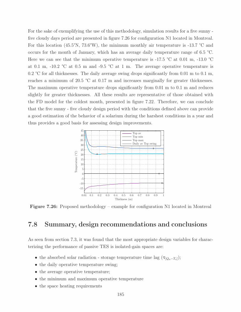
For the sake of exemplifying the use of this methodology, simulation results for a five sunny -

five cloudy days period are presented in figure 7.26 for configuration N1 located in Montreal.

For this location (45.5°N, 73.6°W), the minimum monthly air temperature is -13.7 °C and

occurs for the month of January, which has an average daily temperature range of 6.5 °C.

Here we can see that the minimum operative temperature is -17.5 °C at 0.01 m, -13.0 °C

at 0.1 m, -10.2 °C at 0.5 m and -9.5 °C at 1 m. The average operative temperature is

0.2 °C for all thicknesses. The daily average swing drops significantly from 0.01 m to 0.1 m,

reaches a minimum of 20.5 °C at 0.17 m and increases marginally for greater thicknesses.

The maximum operative temperature drops significantly from 0.01 m to 0.1 m and reduces

slightly for greater thicknesses. All these results are representative of those obtained with

the FD model for the coldest month, presented in figure 7.22. Therefore, we can conclude

that the five sunny - five cloudy design period with the conditions defined above can provide

a good estimation of the behavior of a solarium during the harshest conditions in a year and

thus provides a good basis for assessing design improvements.

Thickness (m)

Tem

per

atur

e(°

C)

Top avTop minTop maxDaily av Top swing

0.01 0.1 0.2 0.3 0.4 0.5 0.6 0.7 0.8 0.9 1

-15

-10

-5

0

5

10

15

20

25

30

35

40

45

Figure 7.26: Proposed methodology – example for configuration N1 located in Montreal

7.8 Summary, design recommendations and conclusions

As seen from section 7.3, it was found that the most appropriate design variables for charac-

terizing the performance of passive TES is isolated-gain spaces are:

• the absorbed solar radiation - storage temperature time lag (τ[Qa−Ts]);

• the daily operative temperature swing;

• the average operative temperature;

• the minimum and maximum operative temperature

• the space heating requirements

185

The key design targets of solaria/greenhouses equipped with various passive TES systems

have been analyzed with frequency response (FR) and finite difference thermal network (FD)

models. Upon analysis of the simulation results obtained with these models, within the

main performance parameters identified above, we can conclude that passive TES in solaria

and greenhouses can most significantly impact the timing of the heat delivery (as captured

by τ[Qa−Ts]), the daily average operative temperature swing and the minimum operative

temperature. Therefore we suggest focusing on these three design targets when designing

TES in solaria and greenhouses.

As seen from figure 7.7c, the presence of a storage mass on the north wall or the floor

significantly reduces the daily operative temperature swing up to a thickness about 0.10-

0.20 m and becomes mostly constant beyond – under the periodic conditions of a cold sunny

day. This behavior is mostly independent of the design period under consideration. Results

obtained with the FD model with real weather data confirmed this observation and revealed

an annual daily swing minimum around 0.20 m with minimal increase for greater thickness.

Therefore, it is recommended to adopt a TES with a thickness of at least 0.15 m for reducing

temperature swings.

Under periodic conditions, the minimum operative temperature is strongly affected by the

design period under consideration (see figure 7.13a). Simulations with the FD model with

real weather data revealed an ever increasing minimum temperature with storage thickness –

at least up to 1 m. However, the slope of the minimum operative temperature changes with

an inflection point at about 0.20-0.30 m; therefore the biggest contribution for raising the

minimum operative temperature are made up to that point, where the minimum tempera-

ture keeps increasing beyond but less markedly. Result obtained with the FD model revealed

that increasing the thickness of TES from 0.10 m to 1 m can raise the minimum tempera-

ture in unheated solaria and greenhouses by 3 to 5 °C, depending on the configuration and

weather conditions. For raising the minimum operative temperature in heated solaria and

greenhouses, it is recommended to select a TES thickness of about 0.25 m. For unheated

solaria and greenhouses, it is recommended to select a TES with a minimum thickness of

0.3 m and even thicker if allowable by space constraints. For a fixed thickness of thermal

mass, it is recommended to place about 0.10 m on the floor and the remaining on the north

wall.

As seen in figure 7.7e, it is not possible to design the thickness of a passive TES system to

provide a time lag appropriate for night cooling. It is however possible to improve thermal

comfort in the evening by selecting a TES thickness with a high τ[Qa−Ts]. If providing comfort

during the evening is an important design goal, it is recommended to implement a TES on

186

the north wall or the floor with a thickness between 0.05-0.10 m and to select a configuration

with opaque north, east and west walls. Implementing a 6 cm TES on both the north wall

and the floor maximizes τ[Qa−Ts] for both TES and is thus the best option for improving

evening thermal comfort.

If providing evening warmth and higher minimum temperatures are both important design

goals, it is suggested to select a configuration with a massive floor and north wall and insulated

east and west walls (i.e. configuration FN2) and to locate a 0.06-0.08 m TES on the floor

and a TES on the north wall as thick as possible while meeting practical constraints. The

use of water as TES material should be considered.

The average operative temperature under a periodic sunny day in winter remains mostly

constant with thicknesses between 0.01 m and 1 m. Under real weather conditions, the

monthly average temperature exhibited a seasonal behavior where the average temperature

of December increased with thickness, remained mostly constant in January and reduced with

thickness in February. Thus we may conclude that large passive TES tend to increase the

average temperature in early winter and to decrease it in late winter. With increased solar

availability in February compared to December, this could be an acceptable drawback.

As seen in figure 7.13a, increasing the storage thickness to about 0.10 m significantly reduces

the maximum operative temperature under a periodic sunny winter day. The analysis under

real weather conditions revealed a further reduction until a thickness of about 0.20 m for most

months and varying results beyond. Regardless of the TES thickness, additional measures

should be implemented to prevent overheating such as ventilation and the use of shading

devices.

A reduction of the thermal resistance of the insulation layer behind the storage mass from

RSI 20 to RSI 2 was found to reduce the average operative temperature of winter months by

about 0.5 °C independently of the TES thickness, while a greater reduction of the minimum

temperature was observed for lower thicknesses. It is recommended to analyze the effects of

varying the insulation level at the end of the design process, when most of the key design

variables have been selected.

The introduction of continuous indoor air recirculation increases convective exchanges and

can significantly reduces the maximum operative temperature, but reduces slightly its average

and minimum temperature as well as τ[Qa−Ts]; it is thus recommended to use indoor fans on

an intermittent basis.

187

It was found the use of water as TES material instead of concrete or soil can significantly re-

duce the daily average operative temperature swing and peak temperatures as well as increase

τ[Qa−Ts]. Therefore, including water in solaria and greenhouses is recommended.

Although most simulation results presented here were obtained for a 24 m2 solarium with

specific dimensions, it was shown that spaces with different dimensions have similar optimal

TES thicknesses for the main output variables; thus, results presented here can be valuable

for designing solaria and greenhouses with different dimensions.

This chapter presented a methodology for sizing passive TES in solaria and greenhouses that

can be used for reaching different design intents. Future studies should focus on improving

the efficiency of large TES in isolated-gain spaces, where the use of active ventilation and the

development of efficient strategies for controlling the airflow is of particular interest.

188

Chapter 8

Conclusion

8.1 Summary

This Ph.D. thesis presented a wide literature review on various aspects related to the design

and control of solaria and greenhouses. Relevant studies conducted on geometrical parame-

ters and orientation, glazing and shading materials, thermal energy storage and innovative

auxiliary heating systems were presented.

The four main variables governing the interior climate are the indoor temperature, relative

humidity, CO2 concentration and solar radiation level. These variables must be controlled to

maintain production objectives, energy consumption targets or thermal comfort for people

and plants. Different systems can be employed to modify these variables, such as shading and

ventilation systems, auxiliary heating systems, dehumidification, CO2 injection and artificial

lighting systems. The impacts of these systems on the main variables have been discussed.

Different climate control strategies were reviewed and the best climate control models were

presented.

Based on this review of the scientific literature, the following recommendations are pro-

posed:

• A design with a high aspect ratio must be preferred, with the longest side facing south.

• If possible, the south roof angle should be slightly higher than the latitude (+5-20°).

• The north wall should be opaque and have a thermally massive material as inner layer.

• Ventilation openings should be provided along the longest side, with both roof vents

and side vents.

189

• Both roof and side vents should be used for summer ventilation, while only the side

vents or roof vents should be used for winter ventilation.

• Due to its durability and aesthetic, glass should be the preferred glazing material for

building-integrated solaria and greenhouses.

• When glass is the selected cover material, the use of anti reflecting and low emissivity

coatings as well as argon filling should be considered.

• Increasing the number of layers of the glazing material is highly desirable for reducing

heat losses.

• At least one shading device should be installed; two is even better.

• The floor inside layer should have appreciable thermal storage capacity and have insu-

lation as external layer.

• Including animals or composting installations in solaria and greenhouse should be en-

visioned for their heat and CO2 production, where they should be selected based on

carbon dioxide needs.

• If artificial lighting is used, CO2 enrichment should be practiced simultaneously.

• If plants are grown in the space, the use of a ventilation system with heat recovery

should be considered for humidity control in winter instead of natural ventilation.

The energy saving potential of attached solaria and greenhouses has been evaluated in chapter

3 for the province of Québec, Canada. It was found that solaria can collect significant surplus

heat that can be transferred to an adjacent house to partly offset its heating load. Results

obtained from the different solarium configurations revealed that a net energy balance of 28-

144 kWh/m2 of solarium floor area is possible. Retrofitting an energy efficient solarium to an

average house could reduce its heating demand by 9% to 23%, depending on the size of the

solarium. In these simulations, the solarium was conditioned with a heating set point of 10 °C

and the heat was available for the house when the temperature inside the solarium exceeded

28 °C. Simulations conducted for large rooftop greenhouses revealed that achieving net zero

heating is possible and that surplus heat up to 31 kWh/m2 of greenhouse floor area can be

collected with an energy efficient design (with a heating set point of 15 °C and surplus heat

when the temperature is exceeding 25°C). Covering 1% of large commercial and institutional

buildings in Quebec with rooftop greenhouses could provide enough vegetables to feed 300

000 people without increasing the total energy consumption of the province.

A methodology for the design of fenestration systems in heating dominated climates has

been developed and is presented in chapter 5. This methodology can be used at the early

design stage for providing assistance in the selection of glazings or windows equipped with

190

shading devices. The solar and thermal effects resulting from the presence of an interior

and/or exterior planar shade, parallel to the glass, can be simulated. Diagrams displaying

the annual energy gain (or loss) per unit area as a function of the effective U-value and solar

heat gain coefficient of a fenestration system are generated, for a specific surface orientation

and climate. Such diagrams are useful at the early design stage when there is a need to

compare various fenestration systems on a relative basis. This methodology can be used

for designing buildings aiming at a high solar utilization like solaria and greenhouses, where

different fenestrations systems may be selected for different surface orientation in order to

increase the net energy gains of a space.

While the use of one or more shades is suggested by many researchers for reducing heat losses,

the literature review revealed a need for an improved control method. A new control strategy

for improving the operation of an exterior and/or interior planar shade is presented in chapter

6. The control strategy is based on performing an energy balance on the fenestration system

and calculating the total heat flow (i.e. solar gains + overall heat losses). The heat flow

can be maximized or minimized, depending on the needs of the space. A solarium model

was developed to assess the performance of the proposed control method. Simulation results

revealed that a 3-9% reduction of the heating requirements is possible and an additional

9-14% surplus heat can be collected in the heating mode, compared to a control based on

global horizontal solar radiation levels (with a heating set point of 10 °C and surplus heat

considered for a temperature exceeding 28 °C). During the mixed mode, it was shown that

thermal comfort can be significantly improved with an additional 1822 hours within the

thermal comfort range when controlling an interior shade with the proposed algorithm.

A methodology for designing passive thermal energy storage (TES) systems has been de-

veloped and is presented in chapter 7. Potential targets for thermal mass design strategies

were reviewed, along with common metrics used in the characterization of the performance of

TES systems. Six different solarium/greenhouse designs were investigated, which encompass

the most frequent configurations. Two complementary modelling approaches were considered

for analyzing these configurations: frequency response (FR) and finite difference (FD). The

frequency response models were used for sensitivity studies used under short periodic con-

ditions while FD models were used in full-year performance assessments with real weather

data. Many design variations have been considered with these models, which allowed to

formulate design recommendations. A methodology based on a frequency response model

was presented for sizing TES in solaria and greenhouses. The methodology is applicable to

various solaria and greenhouse designs with the energy balance equations corresponding to

six different configurations that are provided.

191

8.2 Contributions

Upon reviewing the scientific literature pertaining to the design and control of solaria and

greenhouses, many research opportunities have been identified and some of them were tackled.

The major contributions of this thesis are:

• The evaluation of the energy potential of attached solaria and rooftop greenhouses for

the province of Québec.

• The development of a methodology for selecting fenestration systems with a high solar

energy utilization.

• The elaboration of a new control algorithm for improving the control of multiple shading

devices that can maximize or minimize the total heat flow, depending on the needs of

the space.

• The development of a methodology for sizing TES in solaria and greenhouses that is

applicable to various designs and climates.

8.3 Limitations and outlook

The methodology for selecting fenestration systems is intended for the design of buildings

aiming at a high solar utilization, such as solaria and greenhouses, solar houses and other

kind of buildings where a solar optimized fenestration systems approach has been adopted.

This concept designate a design approach where the role of windows is to maximize the net

energy balance and the role of shading devices is to control overheating and glare issues as

well as improving the energy balance. During the design process, it is recommended to first

use this methodology for identifying the most appropriate glazing and shading combination

for each orientation so as to maximize the solar energy utilization from the fenestration

system. For ensuring a good design, it is necessary thereafter to follow passive solar design

guidelines to adequately position and size windows and select appropriate shading devices to

avoid overheating issues.

Since this methodology is based on steady state calculations, it is not meant to predict

the yearly total energy gained or loss through a fenestration but rather to assist the design

process by comparing the performance of different products on a relative basis. This method-

ology can only evaluate the heat transfer of planar shading elements that are parallel to the

192

glazing. Fixed shadings such as overhangs, fins and louvres cannot be evaluated with this

methodology.

The control strategy for improving the operation of multiple shades presented in this thesis

was developed to be used in solaria and greenhouses. It can also be applicable to residential

buildings for maximizing the solar energy utilization from glazed surfaces, where occupants

override should be allowed to provide for glare and privacy issues. The control algorithm

could also be included as an additional criteria in existing control strategies for office buildings

based on visual comfort. More research is needed in this area for evaluating its energy saving

potential in this context. The assessment of the performance of this control strategy for

other shading types is also desirable. Here again, only planar shading elements parallel to

the glazing are compatible with this control strategy.

The control strategy for operating shades was developed in Matlab and its performance was

assessed with simulations. To use this control strategy in real applications, it is necessary to

develop an approximate model for real-time control. To this aim, transfer functions should be

elaborated based on three inputs: the incident solar radiation level, the exterior temperature

and the interior temperature. Developing a method for deriving these transfer functions

for different designs and climates is needed for the real-time implementation of this control

strategy in solaria and greenhouses.

The procedure for calculating the convective heat transfer coefficient in a ventilated cavity

described in ISO15099, based on first principles physical models, is expensive to implement

and lacks experimental validation. The conduction of extensive experimental studies of var-

ious shading materials and configurations and the development of simpler empirical models

are needed.

Extensive simulations of solaria have been performed with frequency response (FR) and fi-

nite difference (FD) models. Comparing these simulation results with experiments would

be a valuable exercise. In particular, performing an experimental comparison of two iden-

tical solaria but with different TES thicknesses and observing the differences between the

main performance variables would be desirable for confirming the validity of the simulation

results.

The methodology for sizing TES in solaria and greenhouses was limited to passive TES.

Expanding this methodology for the design of active TES is an important research objective

that should be pursued in future studies. Ventilated TES allow to increase the effective heat

storage capacity of a mass by enhancing heat transfer; they have the potential to further

reduce extreme temperatures in unheated solaria and greenhouses. Effective control strategies

193

should be developed for controlling the airflow based on various needs, such as limiting

high temperatures and improving the indoor conditions for people and plants, where model

predictive controls could be used to reach these goals.

Although care was taken for proposing a methodology that is accurate, yet simple to imple-

ment, the development of this methodology in a programing software will still require non

negligible efforts from a designer. Integrating this methodology into a design tool that be can

used for the design of solaria and greenhouses would widen its use and thus be a worthwhile

effort.

Innovative greenhouse prototypes have been built with integrated photovoltaics and desali-

nation capabilities; future research on semi transparent photovoltaics and seawater desali-

nation specifically adapted to greenhouses would be highly valuable. Concerning materials

development, further improvement of glass coatings combining very high solar and visible

transmittance as well as shading materials with a high visible transmittance and low near

infra red transmittance would be highly desirable for solaria and greenhouses.

8.4 Final thoughts

Many research needs were identified for improving the design and control of solaria and

greenhouses, from which only a few could be addressed in this thesis. Nevertheless, with

the actual state of knowledge and the existing materials available, it is already possible to

build highly efficient spaces that can provide a great environment where people and plants

can thrive. I believe that the work presented in this thesis can be useful for achieving this.

With a little planning, it is possible to design a space that can provide a nice environment

for people while capturing additional solar heat that can be used by an adjacent building and

producing fresh vegetables simultaneously. Doing so is a step further for a reduced ecological

footprint and increased resilience, in a very pleasant way.

194

References

Aaslyng, J., Lund, J., Ehler, N., Rosenqvist, E., 2003. IntelliGrow: a greenhouse component-based climatecontrol system. Environmental Modelling & Software 18 (7), 657–666.

Aguiar, L., da Costa, J., Aguiar, R., Fischer, G., 2009. Estimates and measurements of photosyntheticallyactive radiation and global solar irradiance in Rondonia. In: AIP Conference proceedings.

Ahmed, M., 2005. Evaluation and optimization of solar desiccant wheel performance. Renewable Energy30 (3), 305–325.

Aikman, D., 1989. Potential increase in photosynthetic efficiency from the redistribution of solar radiation ina crop. Journal of experimental botany 40 (217), 855–864.

Al-Saadi, S. N., Zhai, Z., 2013. Modeling phase change materials embedded in building enclosure: A review.Renewable and Sustainable Energy Reviews 21, 659–673.

Alexandri, E., Jones, P., 2007. Developing a one-dimensional heat and mass transfer algorithm for describingthe effect of green roofs on the built environment: Comparison with experimental results. Building andEnvironment 42 (8), 2835–2849.

American Society of Agricultural Engineers, 2003. Heating, ventilating and cooling greenhouses. ANSI/ASAEEP406.4 JAN03.

Andrusiak, M., Harrison, S., 2009. The modelling and design of a solar-driven liquid-dessicant air-conditioningsystem. In: 4th Annual Canadian Solar Buildings Conference. Toronto.

Asan, H., 2000. Investigation of wall’s optimum insulation position from maximum time lag and minimumdecrement factor point of view. Energy and Buildings 32 (2), 197–203.

Asan, H., 2006. Numerical computation of time lags and decrement factors for different building materials.Building and Environment 41 (5), 615–620.

ASHRAE, 2007. ASHRAE Handbook - HVAC Applications, A44. American Society of Heating, Refrigeratingand Air-Conditioning Engineers, p6.

ASHRAE, 2008. ASHRAE Vision 2020 - Producing net zero energy buildings. American Society of Heating,Refrigerating and Air-Conditioning Engineers.

ASHRAE, 2009. ASHRAE Handbook - Fundamentals. American Society of Heating, Refrigerating and Air-Conditioning Engineers.

Aste, N., Angelotti, A., Buzzetti, M., 2009. The influence of the external walls thermal inertia on the energyperformance of well insulated buildings. Energy and Buildings 41, 1181–1187.

Astee, L. Y., Kishnani, N. T., 2010. Building-integrated agriculture: utilising rooftops for sustainable foodcrop cultivation in Singapore. Journal of Green Building 5 (2), 105–113.

195

Athienitis, A., O’Brien, W., 2015. Modeling, design, and optimization of net-zero energy buildings. JohnWiley & Sons.

Athienitis, A., Stylianou, M., 1991. Method and global relationship for estimation of transmitted solar energydistribution in Passive Solar Room. Energy Sources 13, 319–336.

Athienitis, A., Sullivan, H., 1985. Efficient method for determination of solar radiation absorbed by eachroom interior surface, and effects. In: International Solar Energy Society. pp. 430–434.

Athienitis, A., Sullivan, H., Hollands, K., 1986. Analytical model, sensitivity analysis, and algorithm fortemperature swings in direct gain rooms.

Athienitis, A. K. ., 2007. Design of a solar home with BIPV-thermal system and ground source heat pump.In: 2nd Canadian Solar Buildings Conference. Calgary, pp. 1–9.

Athienitis, A. K., 1994. Building thermal analysis. MathSoft Inc, Cambridge.

Athienitis, A. K., Liu, C., Hawes, D., Banu, D., Feldman, D., 1997. Investigation of the thermal performanceof a passive solar test-room with wall latent heat storage. Building and Environment 32 (5), 405–410.

Athienitis, A. K., Santamouris, M., 2013. Thermal analysis and design of passive solar buildings. Earthscan.

Bailey, B., 1984. Limiting the relative humidity in insulated greenhouses at night. In: III InternationalSymposium on Energy in Protected Cultivation 148. ISHS, pp. 411–420.

Bailey, B., 1988. Control strategies to enhance the performance of greenhouse thermal screens. Journal ofAgricultural Engineering Research 40, 187–198.

Bakker, J., Adams, S., Boulard, T., Montero, J., 2008. Innovative technologies for an efficient use of energy.Acta Horticulturae 801, 49–62.

Balcomb, D., 1983. Prediction of internal temperature swings in direct-gain passive solar buildings. In: SolarWorld Congress. Perth, Australia, p. 6.

Bastien, D., Athienitis, A., 2013. Evaluation of the potential of attached solariums and rooftop greenhousesin Quebec. In: 3rd Climate Change Technology Conference. Montreal, pp. 1–11.

Bastien, D., Athienitis, A. K., 2015. Methodology for selecting fenestration systems in heating dominatedclimates. Applied Energy 154, 1004–1019.

Bastien, D., Dermardiros, V., Athienitis, A. K., 2015. Development of a new control strategy for improvingthe operation of multiple shades in a solarium. Solar Energy 122, 277–292.

Berroug, F., Lakhal, E. K., El Omari, M., Faraji, M., El Qarnia, H., 2011. Thermal performance of agreenhouse with a phase change material north wall. Energy and Buildings 43 (11), 3027–3035.

Beshada, E., Zhang, Q., 2006. Optimizing the design of solar energy greenhouses. In: The Canadian Societyfor Bioengineering. Edmonton.

Beshada, E., Zhang, Q., Boris, R., 2006. Winter performance of a solar energy greenhouse in southernManitoba. Canadian Biosystems Engineering 48, 5.1–5.8.

Böer, K. W., Duffie, J., 1982. Advances in solar energy: an annual review of research and development -volume 1. Springer US.

Bojic, M. L., Loveday, D. L., 1997. The influence on building thermal behavior of the insulation / masonrydistribution in a three-layered construction. Energy and Buildings 26, 153–157.

196

Bony, J., Citherlet, S., 2007. Numerical model and experimental validation of heat storage with phase changematerials. Energy and Buildings 39, 1065–1072.

Bot, G., van de Braak, N., Challa, H., Hemming, S., Rieswijk, T., Straten, G., Verlodt, I., 2005. The solargreenhouse: state of the art in energy saving and sustainable energy supply. Acta Horticulturae 691,501–508.

Bot, G. P. A., 1983. Greenhouse climate: from physical processes to a dynamic model. Ph.D. thesis, Wa-geningen University.

Both, A., 2000. Some thoughts on supplemental lighting for greenhouse crop production. Center for ControlledEnvironment Agriculture.

Boulard, T., Baille, A., may 1995. Modelling of air exchange rate in a greenhouse equipped with continuousroof vents. Journal of Agricultural Engineering Research 61 (1), 37–48.

Boulard, T., Haxaire, R., Lamrani, M. A., Roy, J. C., Jaffrin, A., 1999. Characterization and modelling ofthe air fluxes induced by natural ventilation in a greenhouse. Journal of Agricultural Engineering Research74, 135–144.

Bourdoukan, P., Wurtz, E., Spérandio, M., Joubert, P., 2006. Evaluation du potentiel solaire appliqué à unsystème desiccant cooling. In: IBPSA. Ile de la Réunion, pp. 1–7.

Braun, J. E., 1990. Reducing energy cost and peak electrical demand through optimal control of buildingthermal storage. ASHRAE Transactions 92 (2), 264–273.

Briassoulis, D., Waaijenberg, D., Gratraud, J., von Eslner, B., 1997. Mechanical properties of coveringmaterials for greenhouses: part 1, general overview. Journal of Agricultural Engineering Research 67 (2),81–96.

Buchholz, M., Jochum, P., Zaragoza, G., 2005. Concept for water, heat and food supply from a closedgreenhouse - the watergy project. Acta Horticulturae 691, 509–516.

Bülow-Hübe, H., 2001. Energy-efficient window systems: effects on energy use and daylight in buildings. Phdthesis, Lund University.

Burns, P. J., Han, K., Winn, C., 1991. Dynamic effects of bang-bang control on the thermal performance ofwalls of various constructions. Solar Energy 46 (3), 129–138.

Butti, K., Perlin, J., 1980. Golden thread: 2500 years of solar architecture and technology. Cheshire Books.

Campen, J., 2009. Dehumidification of Greenhouses. Ph.D. thesis, Wageningen University.

Campen, J. B., Bot, G. P. A., de Zwart, H. F., 2003. Dehumidification of greenhouses at northern latitudes.Biosystems Engineering 86 (4), 487–493.

Candanedo, L. M., Athienitis, A., Park, K.-W., 2011. Convective heat transfer coefficients in a building-integrated photovoltaic/thermal system. Journal of Solar Energy Engineering 133 (2), 14.

Caplow, T., Nelkin, J., 2007. Building-integrated greenhouse systems for low energy cooling. In: 2nd PA-LENC Conference and 28th AIVC Conference on Building Low Energy Cooling and Advanced VentilationTechnologies in the 21st Century. Vol. 1. pp. 172–176.

Carbonari, A., Rossi, G., Romagnoni, P., 2001. Optimal orientation and automatic control of external shadingdevices in office buildings. In: 18th Conference on Passive and Low Energy Architecture. Florianópolis,pp. 1–12.

197

Carlini, M., Castellucci, S., 2010. Modelling and simulation for energy production parametric dependence ingreenhouses. Mathematical Problems in Engineering, 1–28.

Carmody, J., Selkowitz, S., Heschong, L., 2000. Residential windows: a guide to new technologies and energyperformance, 2nd Edition. W.W. Norton & Company, New York.

Cascone, G., Arcidiacono, C., D’Emilio, A., Mazzarella, R., 2005. Radiometric properties and field perfor-mances of different greenhouse plastic coverings. Acta Horticulturae 691, 693–700.

Chau, J., Sowlati, T., Sokhansanj, S., Preto, F., Melin, S., Bi, X., 2009. Economic sensitivity of wood biomassutilization for greenhouse heating application. Applied Energy 86 (5), 616–621.

CMHC, 1996. Energy Audits of High-Rise Residential Buildings. Canadian Mortgage and Housing Corpora-tion.

CMHC, 1998. Tap the sun - Passive Solar Techniques and Home Designs. Canadian Mortgage and HousingCorporation.

Cohen, S., Fuchs, M., 1999. Measuring and predicting radiometric properties of reflective shade nets andthermal screens. Journal of Agricultural Engineering Research 73, 245–255.

Critten, D., 1985. A theoretical assessment of the transmissivity of conventional symmetric roofed multispanE-W greenhouses compared with vertical south roofed greenhouses under natural irradiance conditions.Journal of Agricultural Engineering Research 32 (2), 173–183.

Critten, D., 1991. Optimization of CO2 concentration in greenhouses: a modelling analysis for the lettucecrop. Journal of Agricultural Engineering Research (United Kingdom) 48, 261–271.

Critten, D. L., 1983. The evaluation of a computer model to calculate the daily light integral and transmis-sivity of a greenhouse. Journal of Agricultural Engineering Research 28, 545–563.

Critten, D. L., 1984. The effect of geometric transmission configuration on the light of greenhouses. Journalof Agricultural Engineering Research 29, 199–206.

Curcija, C., Yazdanian, M., Kohler, C., Hart, R., Mitchell, R., Vidanovic, S., 2013. Energy savings fromwindow attachments. Lawrence Berkeley National Laboratory, DOE/EE-0969, 102.

Davies, M. G., 1994. The thermal response of an enclosure to periodic excitation: the CIBSE approach.Building and Environment 29 (2), 217–235.

de Halleux, D., 1989. Modèle dynamique des échanges énergétiques des serres: étude théorique et expérimen.Ph.D. thesis, Faculté des sciences agronomiques de Gembloux.

de Halleux, D., Gauthier, L., 1998. Energy consumption due to dehumidification of greenhouses under north-ern latitudes. Journal of Agricultural Engineering Research 69 (1), 35–42.

de Zwart, H. F., 2008. Overall energy analysis of (semi) closed greenhouses. Acta Horticulturae 801, 811–817.

Dieleman, J., Kempkes, F., 2006. Energy screens in tomato: determining the optimal opening strategy. ActaHorticulturae 718, 599–606.

Dieleman, J. A., Hemming, S., 2011. Energy saving: from engineering to crop management. Acta Horticul-turae 893, 65–73.

Dion, L.-M., Lefsrud, M., Orsat, V., aug 2011. Review of CO2 recovery methods from the exhaust gas ofbiomass heating systems for safe enrichment in greenhouses. Biomass and Bioenergy 35 (8), 3422–3432.

Diver, S., 2001. Compost heated greenhouses. ATTRA.

198

Dorais, M., 2003. The use of supplemental lighting for vegetable crop production: light intensity, cropresponse, nutrition, crop management, cultural practices. Canadian Greenhouse Conference, 1–8.

Droege, P., Puri, V., Caplow, T., 2009. 100% Renewable energy autonomy in action - Chapter 12. Earthscan.

Duffie, J., Beckman, W., 2006. Solar engineering of thermal processes, 3rd edition. John Wiley & Sons.

Dumoulin, L., 2009. Les maisons d’ensemble Terre-Ciel : drôlement écolo ! La maison du 21ème siècle (hiver),70–73.

EA Laboratory Committee, 2013. Evaluation of the uncertainty of measurement in calibration. EA-4/02.

ESR U, 2011. ESP-r 11.11. Energy Systems Research Unit, University of Strathclyde, Glasgow.

EU, 2009. All new buildings to be zero energy from 2019. Press release of European Union.

Evola, G., Marletta, L., 2013. A dynamic parameter to describe the thermal response of buildings to radiantheat gains. Energy and Buildings 65, 448–457.

Facchini, U., Marelli, G., Canzi, L., 1983. Solar greenhouses with low energy consumption. Colture Protette12 (11), 31–35.

FAO, 1994. Integrated energy systems in China - Chapter 10. Food and agriculture organization of the UnitedNations, Rome.

Finlayson, E., Arasteh, D., Huizenga, C., Rubin, M., 1993. Window 4.0: Documentation of calculationprocedures. Lawrence Berkeley National Laboratory, CA.

Fisher, D. E., Pedersen, C. O., 1997. Convective Heat Transfer in Building Energy and Thermal LoadCalculations. ASHRAE Transactions 103.

Foderado, L., 2012. To find fields to farm in New York City, just look up. In: The New York Times. July 112012.

Gagliano, A., Patania, F., Nocera, F., Signorello, C., 2014. Assessment of the dynamic thermal performanceof massive buildings. Energy & Buildings 72, 361–370.

Galasiu, A. D., Atif, M. R., MacDonald, R. a., 2004. Impact of window blinds on daylight-linked dimmingand automatic on/off lighting controls. Solar Energy 76 (5), 523–544.

Garzoli, K., 1989. Energy efficient greeenhouses. In: III Energy Saving in Protected Cultivation. ISHS, pp.53–62.

Gaston, K. J., Davies, T. W., Bennie, J., Hopkins, J., 2012. Reducing the ecological consequences of night-time light pollution: options and developments. Journal of Applied Ecology, pp 11.

Gauthier, C., Lacroix, M., Bernier, H., 1997. Numerical simulation of soil heat exchanger-storage systems forgreenhouses. Solar energy 60 (6), 333–346.

Gebhart, B., 1959. A new method for calculating radiant exchanges. ASHRAE Transactions 65, 321–332.

Gelder, A. D., Heuvelink, E., Opdam, J. J. G., 2005. Tomato yield in a closed greenhouse and comparisonwith simulated yields in closed and conventional greenhouses. Acta Horticulturae 691, 549–552.

Giacomelli, G. A., Roberts, W. J., 1993. Greenhouse covering systems. HortTechnology 3 (l).

Gupta, M. J., Chandra, P., 2002. Effect of greenhouse design parameters on conservation of energy forgreenhouse environmental control. Energy 27 (8), 777–797.

199

Gupta, R., 2004. Effect of latitude on weighted solar fraction of north partition wall for various shapes ofsolarium. Building and Environment 39 (5), 547–556.

Hadorn, J.-C., 2005. Thermal energy storage for solar and low-energy buildings. IEA Solar Heating andCooling Task 32, 169.

Hage, M., 2011. Personal communication.

Halden, R. U., 2010. Plastics and health risks. Annual review of public health 31, 179–94.

Hammarberg, E., 2003. Antireflection treatment of low-emitting glazings for energy efficient windows withhigh visible transmittance. Thin Solid Films 442 (1-2), 222–226.

Hand, D., 1984. Crop responses to winter and summer CO2 enrichment. Acta horticulturae 162, 45–61.

Harnett, R., 1975. Study of glasshouse type and orientation. Acta Horticulturae 46, 209–216.

Hasnain, S. M., 1998. Review on sustainable thermal energy storage technologies, part I : heat storagematerials and techniques. Energy Conversion and Management 39 (11).

He, K.-s., Chen, D.-y., Sun, L.-j., Liu, Z.-l., Huang, Z.-y., 2015. The effect of vent openings on the micro-climate inside multi-span greenhouses during summer and winter seasons. Engineering Applications ofComputational Fluid Mechanics 9 (1), 399–410.

Hed, G., Bellander, R., 2006. Mathematical modelling of PCM air heat exchanger. Energy and Buildings38 (2), 82–89.

Hee, W., Alghoul, M., Bakhtyar, B., Elayeb, O., Shameri, M., Alrubaih, M., Sopian, K., 2015. The role ofwindow glazing on daylighting and energy saving in buildings. Renewable and Sustainable Energy Reviews42, 323–343.

Heier, J., Bales, C., Martin, V., 2015. Combining thermal energy storage with buildings - a review. Renewableand Sustainable Energy Reviews 42, 1305–1325.

Hellickson, M., Walker, J., 1983. Ventilation of agricultural structures.

Hemming, S., Kempkes, F., Braak, N. V. D., Dueck, T., Marissen, N., 2006a. Greenhouse cooling by NIR-reflection. Acta horticulturae (719), 97–105.

Hemming, S., Kempkes, F., Mohammadkhani, V., 2007. New glass coatings for high insulating greenhouseswithout light losses - energy saving, crop production and economic potentials. Acta horticulturae 893,217–226.

Hemming, S., van der Braak, N., T, D., Jongschaap, R., Marissen, N., 2006b. Filtering natural light by thegreenhouse covering using model simulations - more production and better plant quality by diffuse light.Acta horticulturae 719, 105–110.

Heuvelink, E., Bakker, M., 2008. Climate and yield in a closed greenhouse. Acta Horticulturae 801, 1083–1092.

Hong, J. H., Park, K. J., Sohn, B. K., 1997. Effect of composting heat from intermittent aerated static pileon the elevation of underground temperature. Applied Engineering in Agriculture 13 (5), 679–683.

Hottel, H., 1976. A simple model for estimating the transmittance of direct solar radiation through clearatmospheres. Solar Energy 18 (2), 129–134.

Howell, J., 1998. A catalog of radiation heat transfer configuration factors, 2nd Edition.URL http://www.me.utexas.edu/~howell/index.html

200

Huang, Y., Niu, J.-l., Chung, T.-m., 2014. Comprehensive analysis on thermal and daylighting performanceof glazing and shading designs on office building envelope in cooling-dominant climates. Applied Energy134, 215–228.

Hutcheon, N., Handegord, G., 1995. Building science for a cold climate. Institute for Research in Construction,Canada.

Hviid, C. A., Nielsen, T. R., Svendsen, S., 2008. Simple tool to evaluate the impact of daylight on buildingenergy consumption. Solar Energy 82 (9), 787–798.

Hydro-Québec, 2015. Simulation énergétique des bâtiments: Weather data.URL https://www.simeb.ca:8443/index_en.jsp

Ibrahim, M., Achard, P., Wurtz, É., Biwole, P. H., 2013. Optimizing insulation-thermal mass wall layerdistribution from maximum time lag and minimum decrement factor point of view. In: Conference ofInternational Building Performance Simulation Association. Chambéry, pp. 870–876.

IEA, 2005. Implementing agreement on energy conservation through energy storage - Annex 17. No. Inter-national Energy Agency.

Ioslovich, I., 1995. Sub-optimal CO2 Enrichment of Greenhouses. Journal of Agricultural Engineering Re-search 60 (2), 117–136.

Ioslovich, I., Seginer, I., 1998. Approximate seasonal optimization of the greenhouse environment for a multivariable tomato model. American Society of Agricultural Engineers 41 (4), 1139–1149.

ISO 10292, 1994. Glass in building - Calculation of steady state U-value (thermal transmittance) of multipleglazing.

ISO 15099, 2003. Thermal performance of windows, doors and shading devices - Detailed calculations.

Jin, X., Zhang, X., Cao, Y., Wang, G., 2012. Thermal performance evaluation of the wall using heat fluxtime lag and decrement factor. Energy and Buildings 47, 369–374.

Jolliet, O., 1993. Modelling of water uptake, transpiration and humidity in greenhouses, and their effects oncrops. In: Greenhouse crop model 328. ISHS.

Jolliet, O., 1994. HORTITRANS, a model for predicting and optimizing humidity and transpiration in green-houses. Journal of agricultural engineering research 57 (1), 23–37.

Jolliet, O., Bailey, B., 1992. The effect of climate on tomato transpiration in greenhouses: measurements andmodels comparison. Agricultural and Forest Meteorology 58 (1-2), 43–62.

Kacira, M., Sase, S., Okushima, L., 2004. Effects of side vents and span numbers on wind-induced naturalventilation of a gothic multi-span greenhouse. JARQ 38 (4), 227–233.

Kacira, M., Short, T. H., Stowell, R., 1998. A CFD evaluation of naturally ventilated, multi-span sawtoothgreenhouses. Transactions of the ASAE 41 (3), 833–836.

Karlsson, J., Roos, A., 2001. Annual energy window performance vs. glazing thermal emittance - The rele-vance of very low emittance values. Thin Solid Films 392 (2), 345–348.

Karlsson, J., Rubin, M., Roos, A., 2001. Evaluation of predictive models for the angle-dependent total solarenergy transmittance of glazing materials. Solar Energy 71 (1), 23–31.

Kaygusuz, K., 1999. The viability of thermal energy storage. Energy Sources 21 (8), 745–755.

Kempkes, F., 2008. NIR-screen as an energy saving measure. FlowerTECH 11 (2), 20–21.

201

Kesik, T., Simpson, M., 2002. Thermal performance of attached sunspaces for canadian houses. In: esim.Montreal, p. 7.

Khalifa, A., Marshall, R., 1990. Validation of heat transfer coefficients on interior building surfaces using areal-sized indoor test cell. International Journal of Heat and Mass Transfer 33 (10), 2219–2236.

Kittas, C., Baille, A., Giaglaras, P., 1999. Influence of covering material and shading on the spectral distri-bution of light in greenhouses. Journal of Agricultural Engineering Research 73, 341–351.

Klein, S. A., al., E., 2010. TRNSYS 17: A transient system simulation program. Solar Energy Laboratory,University of Wisconsin, Madison, USA.URL http://sel.me.wisc.edu/trnsys

Knight, T., 1808. A description of a forcing house for grapes; with observations on the best method ofconstructing houses for other fruits. Transactions of the Horticultural Society of London 1, 99.

Kontoleon, K. J., Bikas, D. K., 2007. The effect of south wall’s outdoor absorption coefficient on time lag ,decrement factor and temperature variations. Energy and Buildings 39, 1011–1018.

Koo, C., Park, S., Hong, T., Park, H. S., 2014. An estimation model for the heating and cooling demand of aresidential building with a different envelope design using the finite element method. Applied Energy 115,205–215.

Korner, O., 2003. Process-based humidity control regime for greenhouse crops. Computers and Electronicsin Agriculture 39 (3), 173–192.

Körner, O., Challa, H., 2003. Design for an improved temperature integration concept in greenhouse cultiva-tion. Computers and Electronics in Agriculture 39 (1), 39–59.

Kosny, J., Petrie, T., Gawin, D., Childs, P., Desjarlais, A., Christian, J., 2001. Thermal mass - energy savingspotential in residential buildings. Buildings Technology Center, ORNL.

Kostov, O., 1995. Cucumber cultivation on some wastes during their aerobic composting. Bioresource Tech-nology 53 (3), 237–242.

Kotey, N., Collins, M., Wright, J. L., Tiang, T., 2009a. A simplified method for calculating the effectivesolar optical properties of a venetian blind layer for building energy simulation. Journal of Solar EnergyEngineering 131 (2), 9.

Kotey, N. A., Wright, J. L., Collins, M. R., 2009b. Determing off-normal solar optical properties of insectscreens. ASHRAE Transactions 115 (1), 10.

Kotey, N. A., Wright, J. L., Collins, M. R., 2009c. Determining off-normal solar optical properties of draperyfabrics. ASHRAE Transactions 115 (2), 15.

Kotey, N. A., Wright, J. L., Collins, M. R., 2009d. Determining off-normal solar optical properties of rollerblinds. ASHRAE Transactions 115 (1), 10.

Kozai, T., 1977a. Direct solar light transmission into multi-span greenhouses. Agricultural Meteorology 18,339–349.

Kozai, T., 1977b. Direct solar light transmission into single-span greenhouses. Agricultural Meteorology 18,327–338.

Kumar, S., Tiwari, G., Sinha, S., 1994. Optimization and comparative thermal evaluation of four differentsolarium-cum-solar houses. Energy Conversion and Management 35 (10), 835–842.

202

Kummert, M., André, P., Nicolas, J., 2001. Optimal heating control in a passive solar commercial building.Solar Energy 69, 103–116.

Kurata, K., Takakura, T., 1991. Underground storage of solar energy for greenhouses heating. I. Analysis ofseasonal storage system by scale and numerical models. American Society of Agricultural Engineers 34 (2),563–569.

Kurklu, A., 1998. Energy storage applications in greenhouses by means of phase change materials (PCMs) :a review. Renewable Energy 13 (1), 89–103.

Kuznik, F., Virgone, J., 2009. Experimental investigation of wallboard containing phase change material:Data for validation of numerical modeling. Energy and Buildings 41, 561–570.

Kuznik, F., Virgone, J., Noel, J., 2008. Optimization of a phase change material wallboard for building use.Applied Thermal Engineering 28, 1291–1298.

Lacis, A., Schmidt, G., Rind, D., Ruedy, R., 2010. Atmospheric CO2: principal control knob governingEarth’s temperature. Science 330, 356–359.

Lamberg, P., Lehtiniemi, R., Henell, A.-M., 2004. Numerical and experimental investigation of melting andfreezing processes in phase change material storage. International Journal of Thermal Sciences 43 (3),277–287.

Laoudi, A., 2009. Thermal modeling of shading devices of windows. ASHRAE Transactions 115 (2), 1–20.

Laverty, C. C., 1983. Multi-purpose energy conserving sunspace. NTIS.

Lawand, T. A., Alward, R., Saulnier, B., Brunet, E., 1975. The development and testing of an environmentallydesigned greenhouse for colder regions. Solar Energy 17, 302–312.

Lawrence, W., 1963. Science and the glasshouse, 3rd Edition. Olivier and Boyd.

LBNL, 2005. RESFEN 5.0 User’s Manual. Lawrence Berkeley National Laboratory.

LBNL, 2012. International glazing database - IGDB v 23.0.

LBNL, 2014. THERM 6.3 / WINDOW 6.3 NFRC Simulation Manual. Lawrence Berkeley National Labora-tory, CA.

Lee, E. S., Selkowitz, S. E., 2006. The New York Times headquarters daylighting mockup: monitored per-formance of the daylighting control system. Energy and Buildings 38 (7), 914–929.

Lee, I., Lee, S., Kim, G., Sung, J., Sung, S., Yoon, Y., 2005. PIV verification of greenhouse ventilation airflows to evaluate CFD accuracy. Transactions of the ASAE 48 (5), 2277–2288.

Lee, I.-b., Short, T. H., Sase, S., Okushima, L., 2000. Evaluation of structural characteristics of naturally ven-tilated multi-span greenhouses using computer simulation. Japan Agricultural Research Quarterly 34 (4),247–256.

Lee, J. W., Jung, H. J., Park, J. Y., Lee, J. B., Yoon, Y., 2013. Optimization of building window system inAsian regions by analyzing solar heat gain and daylighting elements. Renewable Energy 50, 522–531.

Lorenzo, P., Sanchez-Guerrero, M., Medrano, E., Garcia, M., Caparros, I., Coelho, G., Gimenez, M., 2004.Climate control in the summer season - a comparative study of external mobile shading and fog system.Acta horticulturae 659, 189–194.

203

Lorenzo, P., Sanchez-Guerrero, M., Medrano, E., Garcia, M., Caparros, I., Gimenez, M., 2003. Externalgreenhouse mobile shading: effect on microclimate, water use efficiency and yield of a tomato crop grownunder different salinity levels of the nutrient solution. Acta horticulturae 609.

Loudon, J., 1817. Remarks on the construction of hothouses: also, a review of the various methods of buildingthem in foreign countries as well as in england. J Taylor, London.

Loutzenhiser, P., Manz, H., Maxwell, G., 2007. Empirical validations of shading/daylighting/load interactionsin building energy simulation tools. IEA SHC Task 34/ECBCS Annex 43 Project C, 177.

Lund University, 2010. ParaSol 6.6.URL http://www.ebd.lth.se/program/parasol/

Lychnos, G., Davies, P. A., 2008. A solar powered liquid-desiccant cooling system for greenhouses. Actahorticulturae 797, 95–102.

MacCracken, M. M., 2003. Thermal energy storage myths. ASHRAE Journal September, 36–43.

Mackenzie, G., 1815. On the form which the glass of a forcing-house ought to have, in order to receive thegreatest possible quantity of rays from the sun. Transactions of the Horticultural Society of London 2,171–177.

Malquori, L., Pellegrini, P., Tesi, R., 1993. Determination of solar energy transmitted by different greenhousegeometries. In: Colture Protette. pp. 81–85.

Marsh, L., Albright, L., Langhans, R., 1984. Strategies for controlling greenhouse thermal screens. ActaHorticulturae 148, 453–460.

Mccree, K. J., 1971. The measurment of photosynthetically active radiation. Solar Energy 15, 83–87.

Mesquita, L., Harrison, S., Thomey, D., 2006. Modeling of heat and mass transfer in parallel plate liquid-desiccant dehumidifiers. Solar Energy 80 (11), 1475–1482.

Meyer, J., 1981. Energy saving with mobile thermal screens. Acta Horticulturae 115, 677–684.

Meyer, J., 2011. Extremely insulated greenhouse concept with non fossil fuel heating system. Acta horticul-turae 893 (201-208).

Mihalakakou, G., Ferrante, A., 2000. Energy conservation and potential of a sunspace: sensitivity analysis.Energy Conversion and Management 41 (12), 1247–1264.

Mistriotis, A., Bot, G., Picuno, P., Scarascia-Mugnozza, G., 1997. Analysis of the efficiency of greenhouseventilation using computational fluid dynamics. Agricultural and Forest Meteorology 85 (3-4), 217–228.

Montero, J., 2006. Evaporative cooling in greenhouses: effect on microclimate, water use efficiency and plantresponse. Acta horticulturae 719, 373–383.

Mottard, J., Fissore, A., 2007. Thermal simulation of an attached sunspace and its experimental validation.Solar Energy 81 (3), 305–315.

NASA, 2015. Surface meteorology and solar energy data set.URL http://eosweb.larc.nasa.gov/cgi-bin/sse/grid.cgi?uid=3030

Natural Resources Canada, 2002. Commercial and institutional building energy use survey. Office of EnergyEfficiency.

Natural Resources Canada, 2007. Survey of household energy use. Office of Energy Efficiency.

204

Natural Resources Canada, 2008. Commercial & institutional consumption of energy survey. Office of EnergyEfficiency.

Natural Resources Canada, 2015. Comprehensive energy use database.URL http://oee.nrcan.gc.ca/corporate/statistics/neud/dpa/menus/trends/comprehensive_tables/list.cfm

Navarro, L., de Gracia, A., Niall, D., Castell, A., Browne, M., McCormack, S. J., Griffiths, P., Cabeza, L. F.,2015. Thermal energy storage in building integrated thermal systems: A review. Part 2. Integration aspassive system. Renewable Energy.

NFRC 100-2004, 2004. Procedure for determining fenestration product U-factors. National Fenestration Rat-ing Council, 81.

Nielsen, M. V., Svendsen, S., Jensen, L. B., 2011. Quantifying the potential of automated dynamic solarshading in office buildings through integrated simulations of energy and daylight. Solar Energy 85 (5),757–768.

Nielsen, T., Duer, K., Svendsen, S., 2001. Energy performance of glazings and windows. Solar Energy 69 (1),137–143.

Nielsen, T. R., 2005. Simple tool to evaluate energy demand and indoor environment in the early stages ofbuilding design. Solar Energy 78 (1), 73–83.

Nijskens, J., Deltour, J., Coutisse, S., Nisen, A., 1984. Heat transfer through covering materials of green-houses. Agricultural and forest meteorology 33, 193–214.

Nijskens, J., Deltour, J., Coutisse, S., Nisen, A., 1985. Radiation transfer through covering materials, solarand thermal screens of greenhouses. Agricultural and forest meteorology 35, 229–242.

O’brien, W., 2011. Development of a solar house design methodology and its implementation into a designtool. Phd, Concordia University.

Ochoa, C. E., Aries, M. B. C., van Loenen, E. J., Hensen, J. L. M., 2012. Considerations on design optimiza-tion criteria for windows providing low energy consumption and high visual comfort. Applied Energy 95,238–245.

Opdam, J. J. G., Schoonderbeek, G. G., Heller, E. M. B., 2005. Closed greenhouse : a starting point forsustainable entrepreneurship in horticulture. Acta Horticulturae 691, 517–524.

Orsi, A., 2009. An exploration of the impact of fixed shading device geometry on building energy performance.Master, Michigan State University.

Ould Khaoua, S., Bournet, P., Migeon, C., Boulard, T., Chassériaux, G., 2006. Analysis of greenhouseventilation efficiency based on computational fluid dynamics. Biosystems Engineering 95 (1), 83–98.

Ozel, M., 2014. Effect of insulation location on dynamic heat-transfer characteristics of building externalwalls and optimization of insulation thickness. Energy and Buildings 72, 288–295.

Ozel, M. Ã., Pihtili, K., 2007. Optimum location and distribution of insulation layers on building walls withvarious orientations. Building and Environment 42, 3051–3059.

Öztürk, H. H., 2005. Experimental evaluation of energy and exergy efficiency of a seasonal latent heat storagesystem for greenhouse heating. Energy Conversion and Management 46 (9-10), 1523–1542.

Papadakis, G., Briassoulis, D., Scarascia Mugnozza, G., Vox, G., Feuilloley, P., Stoffers, J., 2000. Radiometricand thermal properties of, and thesting methods for, greenhouse covering materials. Journal of AgriculturalEngineering Research 77 (1), 7–38.

205

Parameshwaran, R., Kalaiselvam, S., Harikrishnan, S., Elayaperumal, A., 2012. Sustainable thermal energystorage technologies for buildings: A review. Renewable and Sustainable Energy Reviews 16 (5), 2394–2433.

Parekh, A., Platts, R., Scanada Consultants, 1990. Passive solar potential in Canada: 1990-2010. Efficiencyand Alternative Energy Technology Branch, Energy, Mines and Resources Canada.

Pearson, L. J., Pearson, L., Pearson, C. J., 2010. Sustainable urban agriculture: stocktake and opportunities.International Journal of Agricultural Sustainability 8 (1-2), 7–19.

Pelland, S., Poissant, Y., 2006. An evaluation of the potential of building integrated photovoltaics in Canada.31st Annual Conference of the Solar Energy Society of Canada, 1–8.

Perdigones, A., Garcia, J., Romero, A., Rodriguez, A., Luna, L., Raposo, C., de la Plaza, S., 2008. Coolingstrategies for greenhouses in summer: control of fogging by pulse width modulation. Biosystems Engineer-ing 99 (4), 573–586.

Perez, R., Ineichen, P., Seals, R., Michalsky, J., Stewart, R., 1990. Modeling daylight availability and irradi-ance components from direct and global irradiance. Solar Energy 44 (5), 271–289.

Pfafferott, J., Herkel, S., Kalz, D., Zeuschner, A., 2007. Comparison of low energy office buildings in summerusing different thermal comfort criteria. Energy and Buildings 39 (7), 750–757.

Porteous, C., Ho, H., 1997. Do sunspaces work in Scotland? Lessons learnt from a CEC solar energydemonstration project in Glasgow. International Journal of Ambient Energy 18 (1), 23–35.

Proskiw, G., 2010. Identifying affordable net zero energy housing solutions. CanmetENERGY, Natural Re-sources Canada.

Protégez-vous, 2012. Ce qu’il faut savoir. Mars.URL http://www.protegez-vous.ca/maison-et-environnement/solariums-2012/ce-quil-faut-savoir.html

Qian, T., Dieleman, J. A., Elings, A., 2011. Comparison of climate and production in closed, semi-closed andopen greenhouses. Acta Horticulturae 893, 807–814.

Rempel, A. R., Gates, K., Rempel, A. W., Shaw, B., 2013. Oregon sunspace redesign / build : new prioritiesfor thermal mass. In: Proceedings of the American Solar Energy Society National Conference. Baltimore,pp. 1–8.

Rempel, A. R., Rempel, A. W., 2013. Rocks, clays, water, and salts: highly durable, infinitely rechargeable,eminently controllable thermal batteries for buildings. Geosciences (3), 63–101.

Rifkin, G., 2011. Cash crops under glass and up on the roof. In: The New York Times.

Roberts, W., Mears, D., Simpkins, J., Cipolletti, J., 1981. Movable thermal insulation for greenhouses. In:Proceedings of the National Agricultural Plastics Congress (USA).

Rogalsky, C., 2011. Application of a network solution to complex fenestration systems. Master thesis, Uni-versity of Waterloo.

Rosa, R., Silva, A. M., Miguel, A., 1989. Solar irradiation inside a single span greenhouse. Journal of Agri-cultural Engineering Research 43, 221–229.

Rosencrantz, T., Bulowhube, H., Karlsson, B., Roos, A., 2005. Increased solar energy and daylight utilisationusing anti-reflective coatings in energy-efficient windows. Solar Energy Materials and Solar Cells 89 (2-3),249–260.

206

Rousse, D., Martin, D., Thériault, R., Léveillée, F., Boily, R., 2000. Heat recovery in greenhouses: a practicalsolution. Applied Thermal Engineering 20, 687–706.

Salazar, R., Rojano, A., 2008. A neural network model to predict temperature and relative humidity in agreenhouse. Acta horticulturae 801, 539–545.

Sánchez, J., Rodríguez, F., Guzmán, J., Ruiz Arahal, M., Fernández, M., 2009. Modelling of tomato croptranspiration dynamics for designing new irrigation controllers. Acta horticulturae 893, 729–737.

Santamouris, M., Argiriou, A., Vallindras, M., 1994a. Design and operation of a low energy consumptionpassive solar agricultural greenhouse. Solar energy 52 (5), 371–378.

Santamouris, M., Balaras, C. A., Dascalaki, E., Vallindras, M., 1994b. Passive solar agricultural greenhouses:A worldwide classification and evaluation of technologies and systems used for heating purposes. SolarEnergy 53 (5), 411–426.

Santamouris, M. I., 1993. Active solar agricultural greenhouses. The state of the art. International Journalof Solar Energy 14 (1), 19–32.

Schoenau, G., Lumbis, A., Besant, R., 1990. Thermal performance of four sunspaces in a cold climate. Energyand Buildings 14, 273–286.

Schumman, J., Lee, E. S., Rubinstein, F. M., Selkowitz, S. E., Robinson, A., 2013. Tips for daylighting withwindows: The integrated approach, 2nd Edition. Lawrence Berkeley National Laboratory.

Seginer, I., 1997. Alternative design formulae for the ventilation rate of greenhouses. Journal of AgriculturalEngineering Research 68 (4), 355–365.

Seginer, I., Albright, L., 1980. Rational operation of greenhouse thermal curtains. Transactions of the ASABE23 (5), 1240–1245.

Seginer, I., Shina, G., Albright, L., Marsh, L., 1991. Optimal temperature setpoints for greenhouse lettuce.Journal of Agricultural Engineering Research 49, 209–226.

Selkowitz, S. E., Bazjanac, V., 1979. Thermal performance of managed window systems. In: ASHRAE /DOE Conference on Thermal Performance of the Exterior Envelopes of Buildings. Orlando, p. 19.

Sethi, V., 2009. On the selection of shape and orientation of a greenhouse: Thermal modeling and experi-mental validation. Solar Energy 83 (1), 21–38.

Sethi, V. P., Sharma, S. K., 2008. Survey and evaluation of heating technologies for worldwide agriculturalgreenhouse applications. Solar Energy 82, 832–859.

Shen, E., Hu, J., Patel, M., 2014. Energy and visual comfort analysis of lighting and daylight control strategies.Building and Environment 78, 155–170.

Siegel, R., Howell, J. R., 1981. Thermal radiation heat transfer, 2nd Edition. Hemisphere Publishing Corpo-ration.

Singh, R., Tiwari, G., 2000. Thermal heating of controlled environment greenhouse: a transient analysis.Energy Conversion and Management 41 (5), 505–522.

Soriano, T., Montero, J., Sánchez-Guerrero, M., Medrano, E., Antón, A., Hernández, J., Morales, M., Castilla,N., 2004. A study of direct solar radiation transmission in asymmetrical multi-span greenhouses using scalemodels and simulation models. Biosystems Engineering 88 (2), 243–253.

Stanghellini, C., Van Meurs, T., 1992. Environmental control of greenhouse crop transpiration. Journal ofAgricultural Engineering Research 51, 297–311.

207

Statistics Canada, 2010. Greenhouse, sod and nursery industries. 22-202-X.

Sun, C., Shu, S., Ding, G., Zhang, X., Hu, X., 2013. Investigation of time lags and decrement factors fordifferent building outside temperatures. Energy & Buildings 61, 1–7.

Tabares-velasco, P. C., Christensen, C., Bianchi, M., 2012. Verification and validation of EnergyPlus phasechange material model for opaque wall assemblies. Building and Environment 54, 186–196.

Takebayashi, H., Moriyama, M., aug 2007. Surface heat budget on green roof and high reflection roof formitigation of urban heat island. Building and Environment 42 (8), 2971–2979.

Tamulaitis, G., Duchovskis, P., Bliznikas, Z., Breive, K., Ulinskaite, R., Brazaityte, A., Novičkovas, A.,Žukauskas, A., 2005. High-power light-emitting diode based facility for plant cultivation. Journal of PhysicsD: Applied Physics 38 (17), 3182–3187.

Tantau, H.-J., Meyer, J., Schmidt, U., Bessler, B., 2011. Low energy greenhouse - a system approach. Actahorticulturae (893), 75–84.

Taylor, W., 1995. Living in glasshouses: vegetality and the curvilinear forcing houses of the early nineteenthcentury. Journal of Garden History 15 (4), 206–220.

The Produce News, 2011. Big Box Farms takes locally grown to a new level. September 23 2011.

Thomas, R. B., 1978. The use of specularly-reflecting greenhouses back walls in greenhouses. Journal ofAgricultural Engineering Research 23, 85–97.

Tiwari, G., Gupta, A., 2002. A comparison in performance of greenhouses with various shapes: a parametricstudy. International Journal of Ambient Energy 23 (3), 136–148.

Tiwari, G., Yadav, Y., Lawrence, S., 1988. Performance of a solarium: an analytical study. Building andEnvironment 23 (2), 145–151.

Tong, G., Christopher, D. M., Li, B., 2009. Numerical modelling of temperature variations in a Chinese solargreenhouse. Computers and Electronics in Agriculture 68 (1), 129–139.

Tong, G., Christopher, D. M., Li, T., Wang, T., 2013. Passive solar energy utilization: A review of cross-section building parameter selection for Chinese solar greenhouses. Renewable and Sustainable EnergyReviews 26, 540–548.

Trigui, M., 2000. Strategy for the optimal climate control of greenhouse tomatoes. Ph.D. thesis, McGill.

Tzempelikos, A., 2005. A methodology for integrated daylighting and tharmal analysis of buildings. Phd,Concordia University.

Tzempelikos, A., 2008. A review of optical properties of shading devices. Advances in Building Energy Re-search 2 (1), 211–239.

Tzempelikos, A., Athienitis, A. K., 2007. The impact of shading design and control on building cooling andlighting demand. Solar Energy 81 (3), 369–382.

Tzempelikos, A., Athienitis, A. K., Karava, P., 2007. Simulation of façade and envelope design options for anew institutional building. Solar Energy 81 (9), 1088–1103.

Tzempelikos, A., Shen, H., 2013. Comparative control strategies for roller shades with respect to daylightingand energy performance. Building and Environment 67, 179–192.

Ulgen, K., 2002. Experimental and theoretical investigation of effects of wall’s thermophysical properties ontime lag and decrement factor. Energy and Buildings 34, 273–278.

208

U.S. Department of Energy, 2012. EnergyPlus 7.2.

U.S. Department of Energy, 2013. EnergyPlus Engineering Reference.

U.S. Department of Energy, 2015. EnergyPlus Energy Simulation Software - Weather Data, 2015–03–10.URL http://apps1.eere.energy.gov/buildings/energyplus/weatherdata_about.cfm

Vadiee, A., Martin, V., 2012. Energy management in horticultural applications through the closed greenhouseconcept, state of the art. Renewable and Sustainable Energy Reviews 16 (7), 5087–5100.

Vadiee, A., Martin, V., 2013a. Energy analysis and thermoeconomic assessment of the closed greenhouse -The largest commercial solar building. Applied Energy 102, 1256–1266.

Vadiee, A., Martin, V., 2013b. Thermal energy storage strategies for effective closed greenhouse design.Applied Energy 109, 337–343.

van Moeseke, G., Bruyère, I., De Herde, A., 2007. Impact of control rules on the efficiency of shading devicesand free cooling for office buildings. Building and Environment 42 (2), 784–793.

Van Ooster, A., Van Henten, E., Janssen, E., Bongaerts, E., 2008. Use of supplementary lighting top screensand effects on greenhouse climate and return on investment. Acta horticulturae 801, 645–652.

van Vennhuizen, R., 2006. Cities farming for the future. RUAF Foundation, IDRC and IIRR.

Vanthoor, B. H., Stigter, J. D., van Henten, E. J., Stanghellini, C., de Visser, P. H., Hemming, S., 2012.A methodology for model-based greenhouse design: Part 5, greenhouse design optimisation for southern-Spanish and Dutch conditions. Biosystems Engineering 111 (4), 350–368.

Vogel, G., mar 2008. Upending the traditional farm. Science 319, 752–753.

Wall, M., 1995. A design tool for glazed spaces. Part I: description. In: ASHRAE Transactions 101. pp.1261–1271.

Wall, M., 1997. Distribution of solar radiation in glazed spaces and adjacent buildings. A comparison ofsimulation programs. Energy and Buildings 26 (2), 129–135.

Wallin, J., Bastien, D., Claesson, J., 2012. The Influence of energy conservation on the performance of solarthermal systems - a cold country case study. Energy Procedia 30, 1069–1078.

Walton, G., 1979. The application of homogeneous coordinates to shadowing calculations. In: ASHRAETransactions 79. pp. 174–179.

Wang, J., Li, S., Guo, S., Ma, C., Wang, J., Jin, S., 2014. Simulation and optimization of solar greenhousesin Northern Jiangsu Province of China. Energy and Buildings 78, 143–152.

Wang, S., Boulard, T., jan 2000. Predicting the microclimate in a naturally ventilated plastic house in amediterranean climate. Journal of Agricultural Engineering Research 75, 27–38.

Warrington, I. J., Norton, R. A., 1991. An evaluation of plant growth and development under various dailyquantum integrals. Journal of American Society for Horticultural Science 116 (3), 544–551.

Wienold, J., 2007. Dynamic simulation of blind control strategies for visual comfort and energy balanceanalysis. In: Building Simulation. pp. 1197–1204.

Wilkinson, T., 1809. Observations on the form of hot houses. Transactions of the Horticultural Society ofLondon 1, 161–164.

WinDat, 2004. WIS Version 3.0.1 Help file - converted to pdf document. Window Energy Data Network.

209

Wong, N., Yu, C., 2005. Study of green areas and urban heat island in a tropical city. Habitat International29 (3), 547–558.

Wright, J. L., 1996. A correlation to quantify convective heat transfer between vertical window glazings.ASHRAE Transactions 102 (1), 940–946.

Wright, J. L., Collins, M. R., Kotey, N. A., Barnaby, C. S., 2009. Improving cooling load calculations forfenestration with shading devices. ASHRAE 1311-RP 30329 (404), 95.

Xu, J., Li, Y., Wang, R. Z., Liu, W., 2014. Performance investigation of a solar heating system with under-ground seasonal energy storage for greenhouse application. Energy 67, 63–73.

Yao, J., 2014. An investigation into the impact of movable solar shades on energy, indoor thermal and visualcomfort improvements. Building and Environment 71, 24–32.

Yu, Z. J., Huang, G., Haghighat, F., Li, H., Zhang, G., 2015. Control strategies for integration of thermalenergy storage into buildings: state-of-the-art review. Energy and Buildings.

Yutong, L., Hongxing, Y., 2008. Investigation on solar desiccant dehumidification process for energy conser-vation of central air-conditioning systems. Applied Thermal Engineering 28 (10), 1118–1126.

Zemanchik, N., Choinière, Y., Suchorski-Trembley, A., Munroe, J., Barrington, S., 1991. Optimum buildingorientation for natural ventilation. In: Agricultural Institute of Canada Annual Conference. CanadianSociety of Agricultural Engineering, Fredericton.

Zhang, L., Xu, P., Mao, J., Tang, X., Li, Z., Shi, J., 2015. A low cost seasonal solar soil heat storage systemfor greenhouse heating: design and pilot study. Applied Energy 156, 213–222.

Zhang, Y., 1997. Predicting the microclimate inside a greenhouse: an application of a one-dimensionalnumerical model in an unheated greenhouse. Agricultural and Forest Meteorology 86 (3-4), 291–297.

Zhang, Y., Chen, Q., Zhang, Y., Wang, X., 2013. Exploring buildings’ secrets: the ideal thermophysicalproperties of a building’s wall for energy conservation. International Journal of Heat and Mass Transfer65, 265–273.

210

Appendix A

Estimating solar transmittance and

absorptance

Tables A.1-A.3 were created by selecting glazings with SHGC > 0.5 from the WINDOW

database (LBNL, 2014) and assembled with cavity widths of 12.7 mm. 37 glasses have been

selected for Table A.1. Correlations from Table A.2 and A.3 have been derived from 16

glasses assembled in 48 and 80 configurations.

Table A.1: Estimated solar transmittance and absorptance - single glazing,ho = 20 W/(m2K) - glazings with U<4 W/(m2K) have low-e on surface #2

U SHGC τs α

U> 5.7 SHGC>0.90 SHGC-0.0035 ho

U (SHGC − τs)

0.80<SHGC<0.90 SHGC-0.0205 ho

U (SHGC − τs)

0.645<SHGC<0.80 SHGC-0.1000 ho

U (SHGC − τs)

0.5<SHGC<0.645 SHGC-0.1315 ho

U (SHGC − τs)

U<4 SHGC>0.635 SHGC-0.0239 ho

U (SHGC − τs)

0.5<SHGC<0.635 SHGC-0.0500 ho

U (SHGC − τs)

211

Table A.2: Estimated solar transmittance and absorptances - double glazing,hi = 8 W/(m2K), ho = 25 W/(m2K) - when present, low-e is on surface #3

U SHGC τs α1 α2

Air

U> 2.7 SHGC>0.82 SHGC-0.0097 SHGC−τs+0.0027(hi−U)/hi

U/ho+(hi−U)/hi-0.0027+αo

0.80<SHGC<0.82 SHGC-0.0285 SHGC−τs+0.0090(hi−U)/hi

U/ho+(hi−U)/hi-0.0090+αo

SHGC<0.80 SHGC-0.0467 SHGC−τs+0.0167(hi−U)/hi

U/ho+(hi−U)/hi-0.0167+αo

1.79<U<2.7 all SHGC SHGC-0.1173 SHGC−τs−0.0881(hi−U)/hi

U/ho+(hi−U)/hi0.0881+αo

1.60<U<1.79 all SHGC SHGC-0.0813 SHGC−τs−0.0427(hi−U)/hi

U/ho+(hi−U)/hi0.0427+αo

Argon

U>2.5 SHGC>0.82 SHGC-0.010 SHGC−τs+0.0025(hi−U)/hi

U/ho+(hi−U)/hi-0.0025+αo

0.75<SHGC<0.82 SHGC-0.0396 SHGC−τs+0.0136(hi−U)/hi

U/ho+(hi−U)/hi-0.0136+αo

1.50<U<1.80 all SHGC SHGC-0.1131 SHGC−τs−0.0878(hi−U)/hi

U/ho+(hi−U)/hi0.0878+αo

1.36<U<1.50 all SHGC SHGC-0.0859 SHGC−τs−0.0488(hi−U)/hi

U/ho+(hi−U)/hi0.0488+αo

212

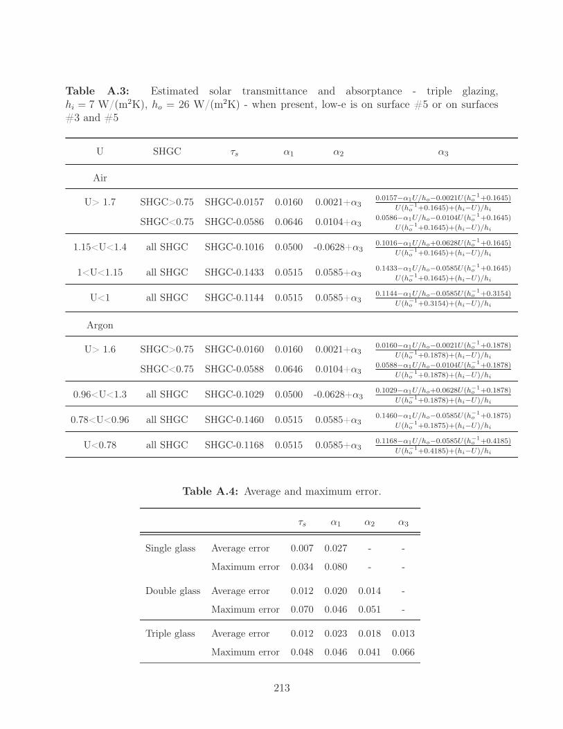
Table A.3: Estimated solar transmittance and absorptance - triple glazing,hi = 7 W/(m2K), ho = 26 W/(m2K) - when present, low-e is on surface #5 or on surfaces#3 and #5

U SHGC τs α1 α2 α3

Air

U> 1.7 SHGC>0.75 SHGC-0.0157 0.0160 0.0021+α30.0157−α1U/ho−0.0021U(h−1

o +0.1645)

U(h−1o +0.1645)+(hi−U)/hi

SHGC<0.75 SHGC-0.0586 0.0646 0.0104+α30.0586−α1U/ho−0.0104U(h−1

o +0.1645)

U(h−1o +0.1645)+(hi−U)/hi

1.15<U<1.4 all SHGC SHGC-0.1016 0.0500 -0.0628+α30.1016−α1U/ho+0.0628U(h−1

o +0.1645)

U(h−1o +0.1645)+(hi−U)/hi

1<U<1.15 all SHGC SHGC-0.1433 0.0515 0.0585+α30.1433−α1U/ho−0.0585U(h−1

o +0.1645)

U(h−1o +0.1645)+(hi−U)/hi

U<1 all SHGC SHGC-0.1144 0.0515 0.0585+α30.1144−α1U/ho−0.0585U(h−1

o +0.3154)

U(h−1o +0.3154)+(hi−U)/hi

Argon

U> 1.6 SHGC>0.75 SHGC-0.0160 0.0160 0.0021+α30.0160−α1U/ho−0.0021U(h−1

o +0.1878)

U(h−1o +0.1878)+(hi−U)/hi

SHGC<0.75 SHGC-0.0588 0.0646 0.0104+α30.0588−α1U/ho−0.0104U(h−1

o +0.1878)

U(h−1o +0.1878)+(hi−U)/hi

0.96<U<1.3 all SHGC SHGC-0.1029 0.0500 -0.0628+α30.1029−α1U/ho+0.0628U(h−1

o +0.1878)

U(h−1o +0.1878)+(hi−U)/hi

0.78<U<0.96 all SHGC SHGC-0.1460 0.0515 0.0585+α30.1460−α1U/ho−0.0585U(h−1

o +0.1875)

U(h−1o +0.1875)+(hi−U)/hi

U<0.78 all SHGC SHGC-0.1168 0.0515 0.0585+α30.1168−α1U/ho−0.0585U(h−1

o +0.4185)

U(h−1o +0.4185)+(hi−U)/hi

Table A.4: Average and maximum error.

τs α1 α2 α3

Single glass Average error 0.007 0.027 - -

Maximum error 0.034 0.080 - -

Double glass Average error 0.012 0.020 0.014 -

Maximum error 0.070 0.046 0.051 -

Triple glass Average error 0.012 0.023 0.018 0.013

Maximum error 0.048 0.046 0.041 0.066

213

Appendix B

Measurement uncertainty for heat

stored/released

The uncertainty associated with the calculation of the heat stored and released has been cal-

culated following the recommendations presented in EA Laboratory Committee (2013).

The heat stored or released has been calculated with

Q = mcp(Tt+1 − Tt) (B.1)

where T in equation B.1 is the bulk temperature of the PCM and the index i refers to the

time interval at which data was recorded (3mn).

The standard uncertainty associated to the mass is equal to 5g. The temperature of the

PCM surface was measured with an accuracy of 0.5°C. Therefore, the standard uncertainty

associated with the calculation of the bulk PCM temperature is√

0.5=0.71°C.

The uncertainty pertaining to the specific heat was estimated by assuming a rectangular

probability distribution between the values provided for melting and freezing. Consequently,

this uncertainty depends on the temperature and is calculated individually for each layer.

For the tested conditions, the minimum and maximum standard uncertainties associated to

the specific heat are equal to 0.66 and 2337 J/(kg°C) with an average of 908 J/(kg°C).

The combined standard uncertainty associated to the heat stored and released by one layer

is calculated as

ΔQ = |Q|√

2(Δm

m

)2

+ 2(Δcp

cp

)2

+(ΔTt+1

Tt+1

)2

+(ΔTt

Tt

)2

(B.2)

The relative standard uncertainty is comprised between 0.03 and 0.79 with an average of

0.16.

214

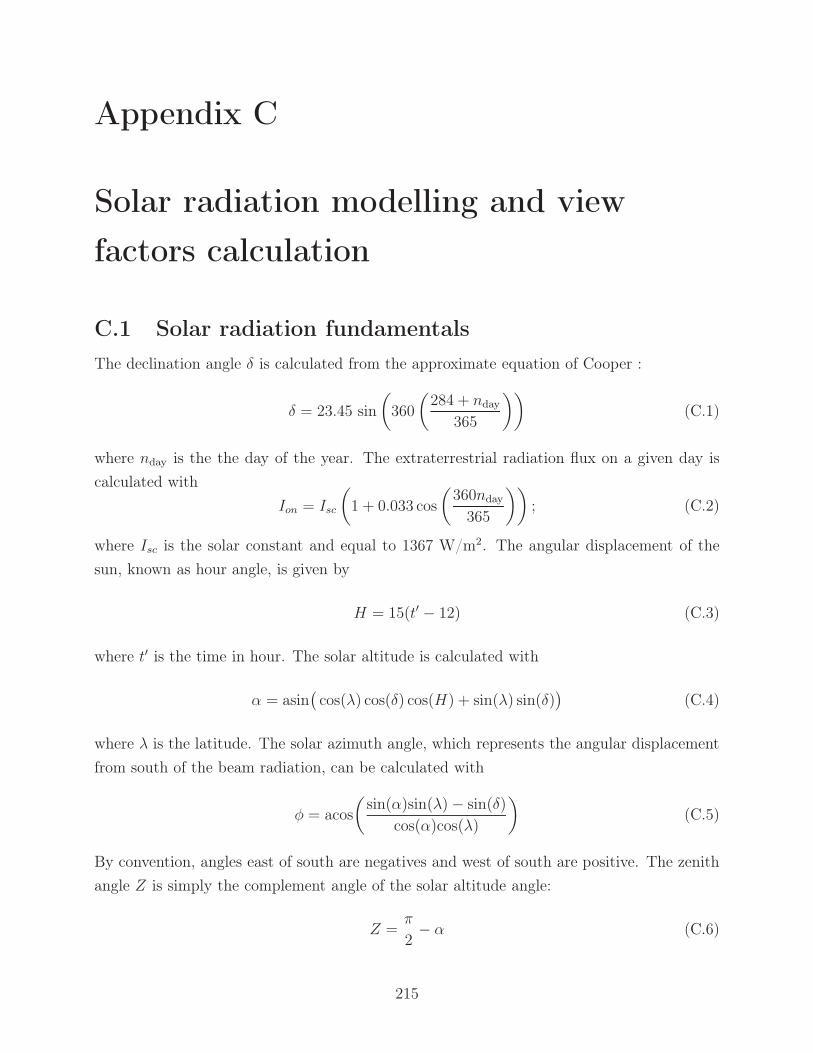
Appendix C

Solar radiation modelling and view

factors calculation

C.1 Solar radiation fundamentals

The declination angle δ is calculated from the approximate equation of Cooper :

δ = 23.45 sin

(360

(284 + nday

365

))(C.1)

where nday is the the day of the year. The extraterrestrial radiation flux on a given day is

calculated with

Ion = Isc

(1 + 0.033 cos

(360nday

365

)); (C.2)

where Isc is the solar constant and equal to 1367 W/m2. The angular displacement of the

sun, known as hour angle, is given by

H = 15(t′ − 12) (C.3)

where t′ is the time in hour. The solar altitude is calculated with

α = asin(cos(λ) cos(δ) cos(H) + sin(λ) sin(δ)

)(C.4)

where λ is the latitude. The solar azimuth angle, which represents the angular displacement

from south of the beam radiation, can be calculated with

φ = acos(

sin(α)sin(λ) − sin(δ)

cos(α)cos(λ)

)(C.5)

By convention, angles east of south are negatives and west of south are positive. The zenith

angle Z is simply the complement angle of the solar altitude angle:

Z =π

2− α (C.6)

215

C.2 Perez model

The diffuse solar radiation in the sky is not uniformly distributed. It can be splitted into

three terms: an isotropic term, uniform throughout the sky dome, a circumsolar diffuse

term, which is concentrated in the region of the sky surrounding the sun, and an horizon

brightening term, which is concentrated near the horizon. The Perez model (1990) presents

a detailed analysis which takes into account these three components. Following this method,

the sky diffuse solar radiation incident on a surface can be calculated with

Ids = DHR(0.5

(1 − F1IR

)(1 + cos(β)

)+ F1IRa/b + F2IRsin(β)

)(C.7)

where F1IR, F2IR, a and b are given by

F1IR = F11IR(εsky) + F12IR(εsky)ΔB + F13IR(εsky)Z (C.8a)

F2IR = F21IR(εsky) + F22IR(εsky)ΔB + F23IR(εsky)Z (C.8b)

a = max(0, cos(θ)

)(C.8c)

b = max(0.087, cos(Z)

)(C.8d)

The clearness of the sky is characterized by εsky and can be calculated with

εsky =(DHR + DNR)/(DHR + kZ3)

1 + kZ3(C.9)

The optical air mass mo can be calculated from

mo =(cos(Z) + 0.50572(96.07995− Z)−1.6364

)−1(C.10)

where Z is in degree. The sky brightness is represented by ΔB and is given by

ΔB = DHR mo/Ion (C.11)

A table with the irradiance coefficients F11IR, F12IR, F13IR, F21IR, F22IR and F23IR as

a function of clearness index can be found in Perez et al. (1990).

216

C.3 View factors

Fij represents the fraction of the radiation emitted by surface i reaching surface j. Because

of energy conservation constraints,N∑

j=1

Fij = 1 (C.12)

where N is the number of surfaces in an enclosure. From the reciprocity principle, it follows

that

A1F12 = A2F21 (C.13)

Howell (1998) published an exhaustive online catalog of configuration factors where the equa-tions presented below can be found; they are given here for the sake of completeness. Theview factor between two rectangles having a common edge perpendicular to each other isgiven by

F12 =1

Wπ

{W tan−1

(1

W

)+ H tan−1

(1

H

)−

√H2 + W 2 tan−1

√1

H2 + W 2

+1

4ln

[((1 + W 2)(1 + H2)

1 + W 2 + H2

)(W 2(1 + W 2 + H2)

(1 + W 2)(W 2 + H2)

)W 2(H2(1 + W 2 + H2)

(1 + H2)(W 2 + H2)

)H2]}

(C.14)

with H = h/l and W = w/l. The dimensions h, w and l as well as the other parametersused in the equations in this section are illustrated in Figure C.1. For two identical, paralleland directly opposed rectangles, the view factor is calculated with

F12 =2

πXY

{ln

((1 + X2)(1 + Y 2)

1 + X2 + Y 2

)1/2

+ X√

1 + Y 2 tan−1

(X√

1 + Y 2

)

+ Y√

1 + X2 tan−1

(Y√

1 + X2

)− Xtan−1(X) − Y tan−1(Y )

}(C.15)

where X = w/z and Y = l/z. The configuration factor for two rectangles having a common

edge separated by an angle α is calculated with

217

F12 =−sin(2α)

4πB

[AB sin(α) +

(π

2− α

)(A2 + B2

)+ B2 tan−1

(A − B cos(α)

B sin(α)

)+ A2 tan−1

(B − Acos(α)

Asin(α)

)]

+sin2

4πB

[(2

sin2(α)− 1

)ln

((1 + A2)(1 + B2)

1 + C

)+ B2 ln

(B2(1 + C)

C (1 + B2)

)+ A2 ln

(A2(1 + A2)cos(2α)

C (1 + C)cos(2α)

)]

+1

πtan−1

(1

B

)+

A

πBtan−1

(1

A

)−

√C

πBatan−1

(1√C

)

+sin(α)sin(2α)

2πBAD

[tan−1

(Acos(α)

D

)+ tan−1

(B − Acos(α)

D

)]

+cos(α)

πB

∫ B

0

√1 + ξ2 sin2(α)

[tan−1

(ξ cos(α)√

1 + ξ2 sin2(α)

)+ tan−1

(A − ξ cos(α)√1 + ξ2 sin2(α)

)]dξ

(C.16)

where A = h/l, B = w/l, C = A2 + B2 − 2ABcos(α) and D =(1 + A2sin2(α)

)1/2. For two

parallel rectangles of different size, the view factor is equal to

F12 =1

(x2 − x1)(y2 − y1)

2∑l=1

2∑k=1

2∑j=1

2∑i=1

(−1)i+j+k+lG(xi, yj, ηk, ξl) (C.17a)

G =1

2π

[(y − η)

√(x − ξ)2 + z2 tan−1

(y − η√

(x − ξ)2 + z2

)

+ (x − ξ)√

(y − η)2 + z2 tan−1

(x − ξ√

(y − η)2 + z2

)− z2

2ln

[(x − ξ)2 + (y − η)2 + z2

] ]

(C.17b)

For two rectangles of different size with an angle α between them that do not share a commonedge, the view factor is given by

F12 =1

(x2 − x1)(y2 − y1)

2∑k=1

2∑j=1

2∑i=1

(−1)i+j+kG(xi, yj , ηk) (C.18a)

G = −(η − y) sin2α

2π

∫ξ

{ ((x − ξcos α) cos α − ξ sin2α√

x2 − 2xξcos α + ξ2 sin2α

)tan−1

(η − y√

x2 − 2xξcos α + ξ2

)

+cos α

(η − y) sin2α

[√ξ2 sin2α + (η − y)2tan−1

(x − ξcos α√

ξ2 sin2α + (η − y)2

)− ξsinα tan−1

(x − ξcos α

sinα

)]

+ξ

2 (η − y)ln

(x2 − 2xξcos α + ξ2 + (η − y)2

x2 − 2xξcos α + ξ2

)}dξ (C.18b)

218

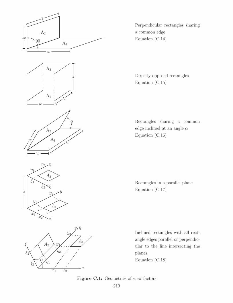
A2

A1

l

h

w

90

Perpendicular rectangles sharing

a common edge

Equation (C.14)

wl

z

A1

A2

Directly opposed rectangles

Equation (C.15)

w

lh

α

A1

A2

Rectangles sharing a common

edge inclined at an angle α

Equation (C.16)

y

x

η

ξz

η2

η1

ξ2

ξ1

y1

y2

x1x2

A2

A1

Rectangles in a parallel plane

Equation (C.17)

y, η

x

ξ

α

y1

y2

x1 x2

ξ1

ξ2

η1

η2

A2

A1

Inclined rectangles with all rect-

angle edges parallel or perpendic-

ular to the line intersecting the

planes

Equation (C.18)

Figure C.1: Geometries of view factors

219

Appendix D

Thermal networks and energy balance

equations for configurations F1, N1, N2,

FN1 and FN2

Figure D.1: Configuration F1 - Thermal network and energy balance equation

��

���

�� ���

��

��

���

�����

��� ���

��

���

��

���

���

��

�����

��

��

��

��

��

�

�

�

��

⎛⎜⎜⎜⎜⎜⎜⎝

sCa+usi+uig+uwi+uvent

−usi −uig −uwi

−usiYs,s+usi+usg+uws

−usg −uws

−uig −usgsCg+uig+usg+

uwg+ug−uwg

−uwi −uws −uwgsCw+uwi+Uws+

uwg+uwo

⎞⎟⎟⎟⎟⎟⎟⎠

⎛⎜⎜⎜⎜⎜⎜⎝

Tin

Ts

Tg

Tw

⎞⎟⎟⎟⎟⎟⎟⎠

=

⎛⎜⎜⎜⎜⎜⎜⎝

Qeq,vent

Ss + Qeq,gr

Sg + Qeq,g

Sw + Qeq,wo

⎞⎟⎟⎟⎟⎟⎟⎠

(D.1)

with Qeq,wo = uwoTo, the other equivalent sources provided in section 7.5.1 and Ys and Yt

given in equations 7.8 and 7.9.

In equations D.2 and D.3, Qeq,o = −YtTo, Qeq,gr = ugrTgr, Qeq,w = uwTo, the other equivalent

sources are provided in section 7.5.1 and Ys and Yt are given in equations 7.8 and 7.9 where

ugr has to be replaced with uo.

220

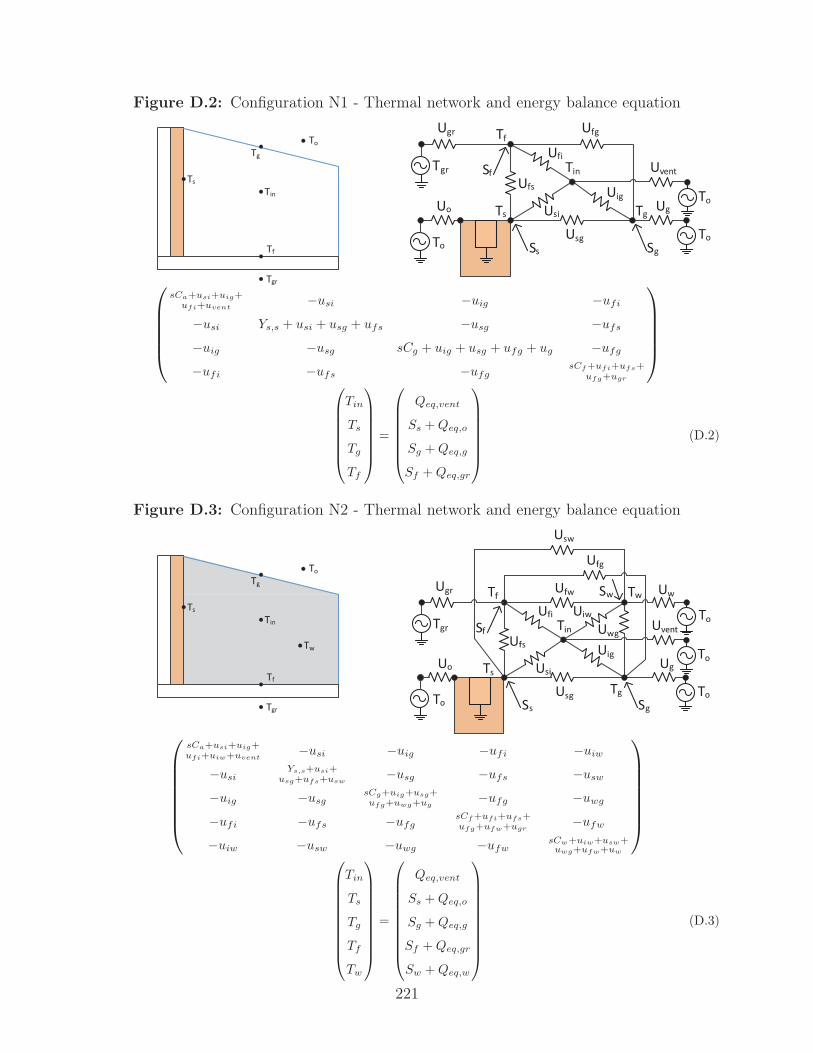
Figure D.2: Configuration N1 - Thermal network and energy balance equation

��

���

��

��

��

�

��

���

��

���

���

��

��

����

��

��

���

���

��

�� �� ��

��

�

�

���

��

⎛⎜⎜⎜⎜⎝

sCa+usi+uig+

ufi+uvent−usi −uig −ufi

−usi Ys,s + usi + usg + ufs −usg −ufs

−uig −usg sCg + uig + usg + ufg + ug −ufg

−ufi −ufs −ufgsCf+ufi+ufs+

ufg+ugr

⎞⎟⎟⎟⎟⎠

⎛⎜⎜⎜⎜⎜⎜⎝

Tin

Ts

Tg

Tf

⎞⎟⎟⎟⎟⎟⎟⎠

=

⎛⎜⎜⎜⎜⎜⎜⎝

Qeq,vent

Ss + Qeq,o

Sg + Qeq,g

Sf + Qeq,gr

⎞⎟⎟⎟⎟⎟⎟⎠

(D.2)

Figure D.3: Configuration N2 - Thermal network and energy balance equation

��

���

��

���

��

��

��

���

�����

���

��

����

���

��

���

���

���

��

���

��

���

��

�� �� ��

��

���

���

�����

���

��

��

��

��

⎛⎜⎜⎜⎜⎜⎜⎝

sCa+usi+uig+

ufi+uiw+uvent−usi −uig −ufi −uiw

−usiYs,s+usi+

usg+ufs+usw−usg −ufs −usw

−uig −usgsCg+uig+usg+

ufg+uwg+ug−ufg −uwg

−ufi −ufs −ufgsCf+ufi+ufs+

ufg+ufw+ugr−ufw

−uiw −usw −uwg −ufwsCw+uiw+usw+

uwg+ufw+uw

⎞⎟⎟⎟⎟⎟⎟⎠

⎛⎜⎜⎜⎜⎜⎜⎜⎜⎜⎝

Tin

Ts

Tg

Tf

Tw

⎞⎟⎟⎟⎟⎟⎟⎟⎟⎟⎠

=

⎛⎜⎜⎜⎜⎜⎜⎜⎜⎜⎝

Qeq,vent

Ss + Qeq,o

Sg + Qeq,g

Sf + Qeq,gr

Sw + Qeq,w

⎞⎟⎟⎟⎟⎟⎟⎟⎟⎟⎠

(D.3)

221

Figure D.4: Configuration FN1 - Thermal network and energy balance equation

���

��

���

��

��

���

���

�����

���

��

����

���

��

���

���

���

��

���

��

���

��

�� �� ��

��

���

���

�����

���

��

��

��

��

⎛⎜⎜⎜⎜⎝

sCa+uSwi+uig

+uSfi+uvent−usi −uig −uSfi

−uSwiYs,Sw+uSwi+

uSwg+uSfSw−uSwg −uSfSw

−uig −uSwgsCg+uig+uSwg+

uSfg+ug−uSfg

−uSfi −uSfSw −uSfgYs,Sf+uSfi+

uSfSw+uSfg

⎞⎟⎟⎟⎟⎠

⎛⎜⎜⎜⎜⎜⎜⎝

Tin

TSw

Tg

TSf

⎞⎟⎟⎟⎟⎟⎟⎠

=

⎛⎜⎜⎜⎜⎜⎜⎝

Qeq,vent

SSw + Qeq,o

Sg + Qeq,g

SSf + Qeq,gr

⎞⎟⎟⎟⎟⎟⎟⎠

(D.4)

Figure D.5: Configuration FN2 - Thermal network and energy balance equation

���

��

���

���

��

��

��

���

�����

���

��

����

���

��

���

���

���

��

���

��

���

��

�� �� ��

��

���

���

�����

���

��

��

��

��

⎛⎜⎜⎜⎜⎜⎜⎝

sCa+uSwi+uig+

uSfi+uiw+uvent−uSwi −uig −uSfi −uiw

−uSwiYs,Sw+uSwi+

uSwg+uSfSw+uSww−uSwg −uSfSw −uSww

−uig −uSwgsCg+uig+uSwg+

uSfg+uwg+ug−uSfg −uwg

−uSfi −uSfSw −uSfgYs,Sf+uSfi+

uSfSw+uSfg+uSfw−uSfw

−uiw −uSww −uwg −uSfwsCw+uiw+uSww+

uwg+USfw+uw

⎞⎟⎟⎟⎟⎟⎟⎠

⎛⎜⎜⎜⎜⎜⎜⎜⎜⎜⎝

Tin

TSw

Tg

TSf

Tw

⎞⎟⎟⎟⎟⎟⎟⎟⎟⎟⎠

=

⎛⎜⎜⎜⎜⎜⎜⎜⎜⎜⎝

Qeq,vent

SSw + Qeq,o

Sg + Qeq,g

SSf + Qeq,gr

Sw + Qeq,w

⎞⎟⎟⎟⎟⎟⎟⎟⎟⎟⎠

(D.5)

222

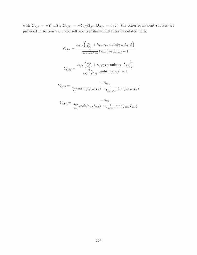
with Qeq,o = −Yt,SwTo, Qeq,gr = −Yt,SfTgr, Qeq,w = uwTo, the other equivalent sources are

provided in section 7.5.1 and self and transfer admittances calculated with:

Ys,Sw =ASw

(uo

ASw+ kSwγSw tanh(γSwLSw)

)uo

kSwγSwASwtanh(γSwLSw) + 1

Ys,Sf =ASf

(ugr

ASf+ kSfγSf tanh(γSfLSf)

)ugr

kSfγSfASftanh(γSfLSf) + 1

Yt,Sw =−ASw

ASw

uocosh(γSwLSw) + 1

kSwγSwsinh(γSwLSw)

Yt,Sf =−ASf

ASf

ugrcosh(γSfLSf ) + 1

kSfγSfsinh(γSfLSf )

223

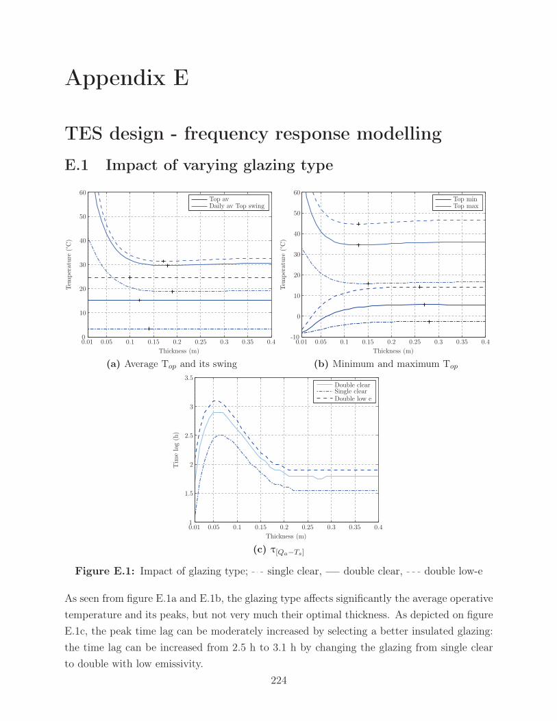
Appendix E

TES design - frequency response modelling

E.1 Impact of varying glazing type

Thickness (m)

Tem

per

atur

e(°

C)

Top avDaily av Top swing

0.01 0.05 0.1 0.15 0.2 0.25 0.3 0.35 0.40

10

20

30

40

50

60

(a) Average Top and its swing

Thickness (m)

Tem

per

atur

e(°

C)

Top minTop max

0.01 0.05 0.1 0.15 0.2 0.25 0.3 0.35 0.4-10

0

10

20

30

40

50

60

(b) Minimum and maximum Top

Thickness (m)

Tim

ela

g(h

)

Double clearSingle clearDouble low e

0.01 0.05 0.1 0.15 0.2 0.25 0.3 0.35 0.41

1.5

2

2.5

3

3.5

(c) τ[Qa−Ts]

Figure E.1: Impact of glazing type; single clear, double clear, double low-e

As seen from figure E.1a and E.1b, the glazing type affects significantly the average operative

temperature and its peaks, but not very much their optimal thickness. As depicted on figure

E.1c, the peak time lag can be moderately increased by selecting a better insulated glazing:

the time lag can be increased from 2.5 h to 3.1 h by changing the glazing from single clear

to double with low emissivity.

224

E.2 Impact of enhanced thermal coupling

Ventilation in greenhouses is beneficial for minimizing temperature, moisture and CO2 gra-

dients. A total air flow of 0.01 m3/s-m2 of floor area is recommended (American Society of

Agricultural Engineers, 2003). Using the correlation from Fisher and Pedersen (1997) for the

geometry under consideration yields convective coefficients of 5.2 W/m2-K for the floor and

11.4 W/m2-K for the wall. The same coefficient as the wall is adopted for the glazing. The

convective coefficients under natural convection were between 3.2-3.3 W/m2-K for the floor,

2.3-2.4 for the wall and 7.3-7.6 W/m2-K for the glazing, depending on the configuration.

Thickness (m)

Tem

per

atur

e(°

C)

Top avTop minTop maxDaily av Top swing

0.01 0.05 0.1 0.15 0.2 0.25 0.3 0.35 0.4-10

0

10

20

30

40

50

60

70

80

(a) Top peaks, average and its swing

Thickness (m)

Tim

ela

g(h

)

Natural convectionForced convection

0.01 0.05 0.1 0.15 0.2 0.25 0.3 0.35 0.41.6

1.8

2

2.2

2.4

2.6

2.8

3

(b) τ[Qa−Ts]

Figure E.2: Impact of enhanced thermal coupling; natural convection, forced con-vection

Enhancing thermal coupling with increased ventilation yields little changes of optimum thick-

nesses for the main performance variables (see figures E.2a-E.2b). Increasing convective heat

exchanges slightly reduces the temperature swing and maximum temperature, but has little

impact on the minimum and average temperatures. It enables the effective use of a slightly

thicker thermal mass: the optimal thickness is 0.01-0.02 m thicker for all configurations,

with a greater impact when the mass is located on the wall (results not shown). However,

introducing forced ventilation also reduces slightly τ[Qa−Ts].

225

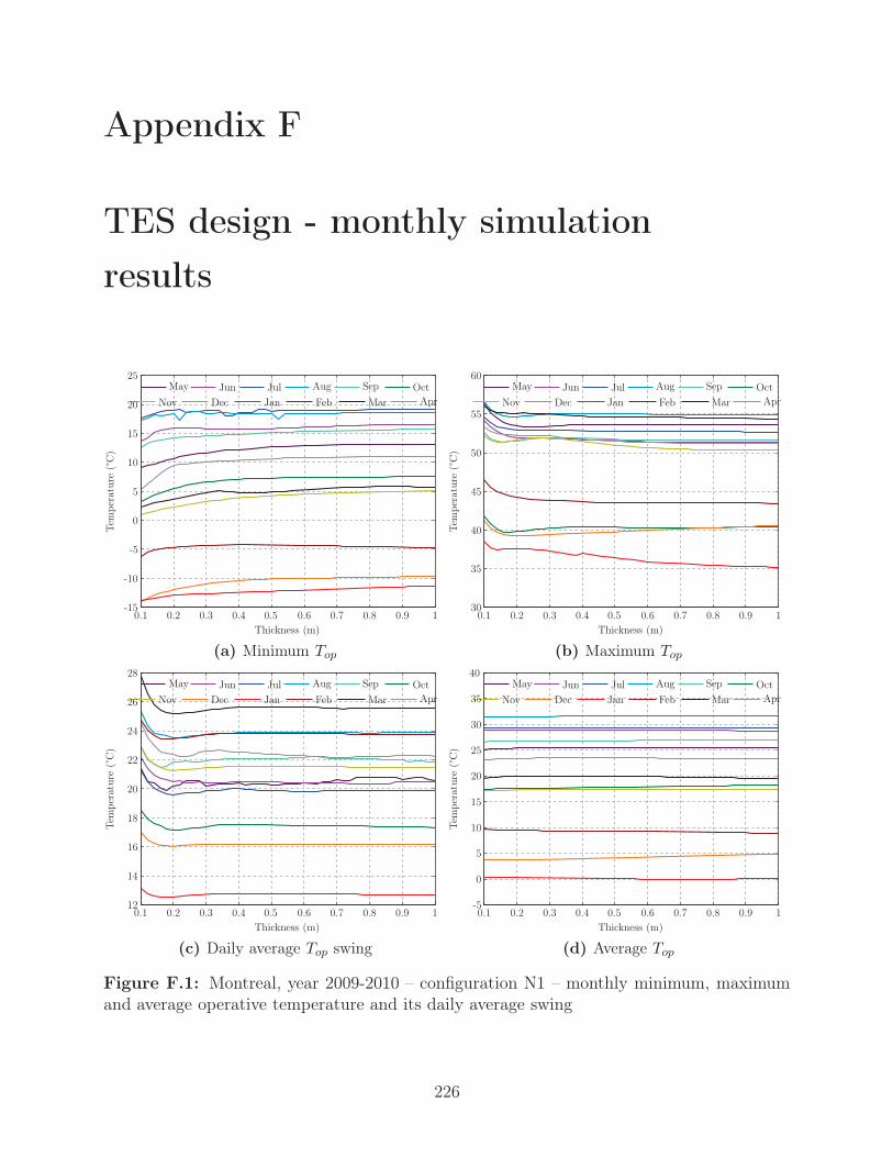
Appendix F

TES design - monthly simulation

results

Thickness (m)

Tem

per

atur

e(°

C)

May Jun Jul Aug Sep Oct

Nov Dec Jan Feb Mar Apr

0.1 0.2 0.3 0.4 0.5 0.6 0.7 0.8 0.9 1-15

-10

-5

0

5

10

15

20

25

(a) Minimum Top

Thickness (m)

Tem

per

atur

e(°

C)

May Jun Jul Aug Sep OctNov Dec Jan Feb Mar Apr

0.1 0.2 0.3 0.4 0.5 0.6 0.7 0.8 0.9 130

35

40

45

50

55

60

(b) Maximum Top

Thickness (m)

Tem

per

atur

e(°

C)

May Jun Jul Aug Sep OctNov Dec Jan Feb Mar Apr

0.1 0.2 0.3 0.4 0.5 0.6 0.7 0.8 0.9 112

14

16

18

20

22

24

26

28

(c) Daily average Top swing

Thickness (m)

Tem

per

atur

e(°

C)

May Jun Jul Aug Sep Oct

Nov Dec Jan Feb Mar Apr

0.1 0.2 0.3 0.4 0.5 0.6 0.7 0.8 0.9 1-5

0

5

10

15

20

25

30

35

40

(d) Average Top

Figure F.1: Montreal, year 2009-2010 – configuration N1 – monthly minimum, maximumand average operative temperature and its daily average swing

226

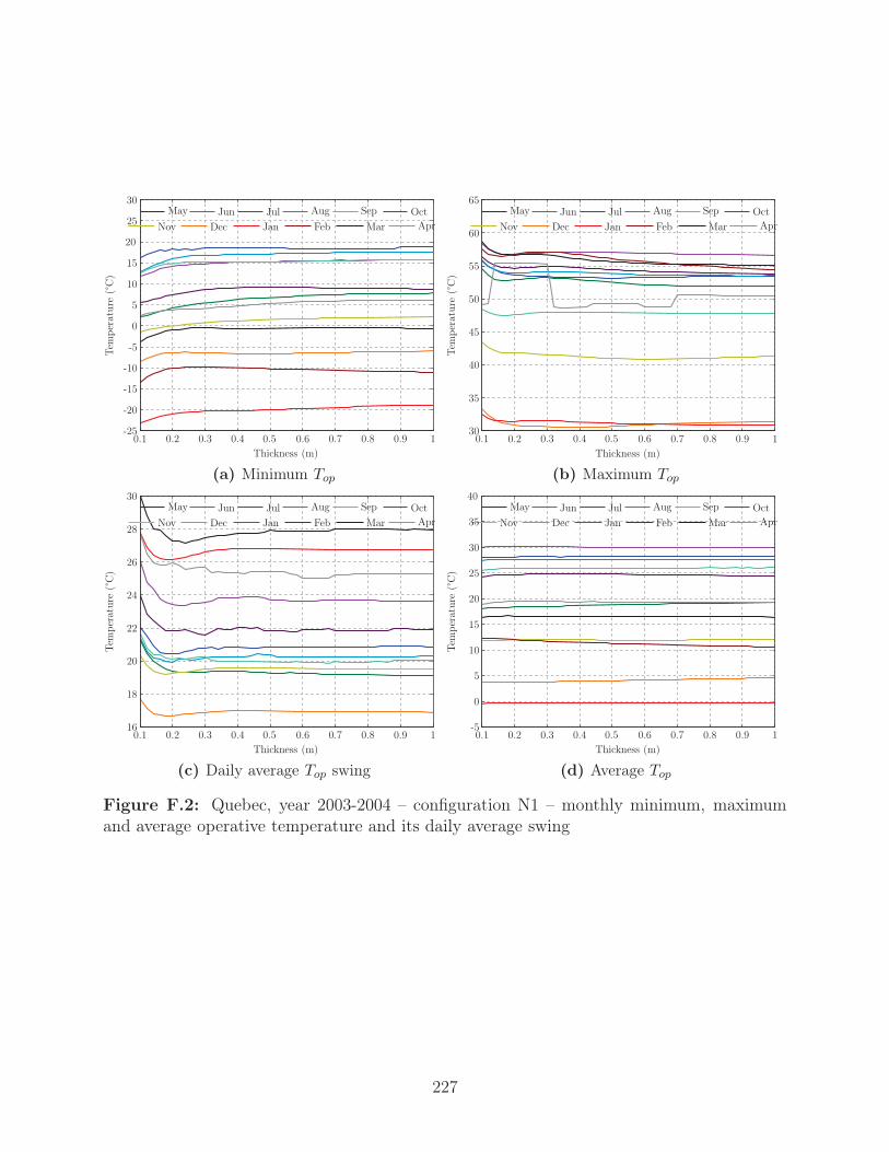
Thickness (m)

Tem

per

atur

e(°

C)

May Jun Jul Aug Sep OctNov Dec Jan Feb Mar Apr

0.1 0.2 0.3 0.4 0.5 0.6 0.7 0.8 0.9 1-25

-20

-15

-10

-5

0

5

10

15

20

25

30

(a) Minimum Top

Thickness (m)Tem

per

atur

e(°

C)

May Jun Jul Aug Sep OctNov Dec Jan Feb Mar Apr

0.1 0.2 0.3 0.4 0.5 0.6 0.7 0.8 0.9 130

35

40

45

50

55

60

65

(b) Maximum Top

Thickness (m)

Tem

per

atur

e(°

C)

May Jun Jul Aug Sep OctNov Dec Jan Feb Mar Apr

0.1 0.2 0.3 0.4 0.5 0.6 0.7 0.8 0.9 116

18

20

22

24

26

28

30

(c) Daily average Top swing

Thickness (m)

Tem

per

atur

e(°

C)

May Jun Jul Aug Sep Oct

Nov Dec Jan Feb Mar Apr

0.1 0.2 0.3 0.4 0.5 0.6 0.7 0.8 0.9 1-5

0

5

10

15

20

25

30

35

40

(d) Average Top

Figure F.2: Quebec, year 2003-2004 – configuration N1 – monthly minimum, maximumand average operative temperature and its daily average swing

227

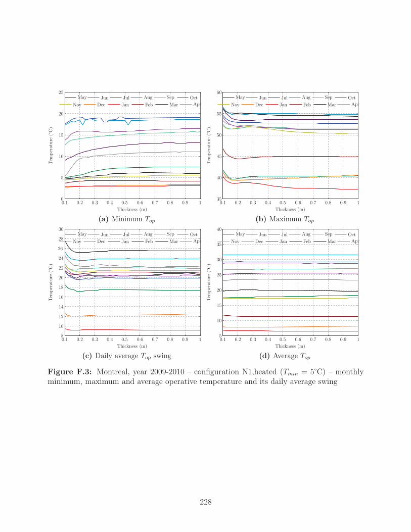
Thickness (m)

Tem

per

atur

e(°

C)

May Jun Jul Aug Sep Oct

Nov Dec Jan Feb Mar Apr

0.1 0.2 0.3 0.4 0.5 0.6 0.7 0.8 0.9 10

5

10

15

20

25

(a) Minimum Top

Thickness (m)Tem

per

atur

e(°

C)

May Jun Jul Aug Sep Oct

Nov Dec Jan Feb Mar Apr

0.1 0.2 0.3 0.4 0.5 0.6 0.7 0.8 0.9 135

40

45

50

55

60

(b) Maximum Top

Thickness (m)

Tem

per

atur

e(°

C)

May Jun Jul Aug Sep Oct

Nov Dec Jan Feb Mar Apr

0.1 0.2 0.3 0.4 0.5 0.6 0.7 0.8 0.9 18

10

12

14

16

18

20

22

24

26

28

30

(c) Daily average Top swing

Thickness (m)

Tem

per

atur

e(°

C)

May Jun Jul Aug Sep OctNov Dec Jan Feb Mar Apr

0.1 0.2 0.3 0.4 0.5 0.6 0.7 0.8 0.9 15

10

15

20

25

30

35

40

(d) Average Top

Figure F.3: Montreal, year 2009-2010 – configuration N1,heated (Tmin = 5°C) – monthlyminimum, maximum and average operative temperature and its daily average swing

228

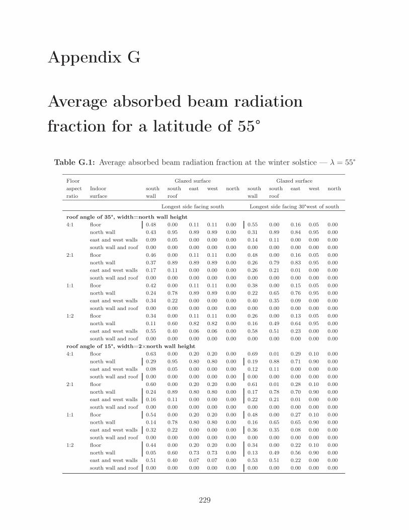
Appendix G

Average absorbed beam radiation

fraction for a latitude of 55°

Table G.1: Average absorbed beam radiation fraction at the winter solstice — λ = 55°

Floor Glazed surface Glazed surface

aspect Indoor south south east west north south south east west north

ratio surface wall roof wall roof

Longest side facing south Longest side facing 30°west of south

roof angle of 35°, width=north wall height

4:1 floor 0.48 0.00 0.11 0.11 0.00 0.55 0.00 0.16 0.05 0.00

north wall 0.43 0.95 0.89 0.89 0.00 0.31 0.89 0.84 0.95 0.00

east and west walls 0.09 0.05 0.00 0.00 0.00 0.14 0.11 0.00 0.00 0.00

south wall and roof 0.00 0.00 0.00 0.00 0.00 0.00 0.00 0.00 0.00 0.00

2:1 floor 0.46 0.00 0.11 0.11 0.00 0.48 0.00 0.16 0.05 0.00

north wall 0.37 0.89 0.89 0.89 0.00 0.26 0.79 0.83 0.95 0.00

east and west walls 0.17 0.11 0.00 0.00 0.00 0.26 0.21 0.01 0.00 0.00

south wall and roof 0.00 0.00 0.00 0.00 0.00 0.00 0.00 0.00 0.00 0.00

1:1 floor 0.42 0.00 0.11 0.11 0.00 0.38 0.00 0.15 0.05 0.00

north wall 0.24 0.78 0.89 0.89 0.00 0.22 0.65 0.76 0.95 0.00

east and west walls 0.34 0.22 0.00 0.00 0.00 0.40 0.35 0.09 0.00 0.00

south wall and roof 0.00 0.00 0.00 0.00 0.00 0.00 0.00 0.00 0.00 0.00

1:2 floor 0.34 0.00 0.11 0.11 0.00 0.26 0.00 0.13 0.05 0.00

north wall 0.11 0.60 0.82 0.82 0.00 0.16 0.49 0.64 0.95 0.00

east and west walls 0.55 0.40 0.06 0.06 0.00 0.58 0.51 0.23 0.00 0.00

south wall and roof 0.00 0.00 0.00 0.00 0.00 0.00 0.00 0.00 0.00 0.00

roof angle of 15°, width=2×north wall height

4:1 floor 0.63 0.00 0.20 0.20 0.00 0.69 0.01 0.29 0.10 0.00

north wall 0.29 0.95 0.80 0.80 0.00 0.19 0.88 0.71 0.90 0.00

east and west walls 0.08 0.05 0.00 0.00 0.00 0.12 0.11 0.00 0.00 0.00

south wall and roof 0.00 0.00 0.00 0.00 0.00 0.00 0.00 0.00 0.00 0.00

2:1 floor 0.60 0.00 0.20 0.20 0.00 0.61 0.01 0.28 0.10 0.00

north wall 0.24 0.89 0.80 0.80 0.00 0.17 0.78 0.70 0.90 0.00

east and west walls 0.16 0.11 0.00 0.00 0.00 0.22 0.21 0.01 0.00 0.00

south wall and roof 0.00 0.00 0.00 0.00 0.00 0.00 0.00 0.00 0.00 0.00

1:1 floor 0.54 0.00 0.20 0.20 0.00 0.48 0.00 0.27 0.10 0.00

north wall 0.14 0.78 0.80 0.80 0.00 0.16 0.65 0.65 0.90 0.00

east and west walls 0.32 0.22 0.00 0.00 0.00 0.36 0.35 0.08 0.00 0.00

south wall and roof 0.00 0.00 0.00 0.00 0.00 0.00 0.00 0.00 0.00 0.00

1:2 floor 0.44 0.00 0.20 0.20 0.00 0.34 0.00 0.22 0.10 0.00

north wall 0.05 0.60 0.73 0.73 0.00 0.13 0.49 0.56 0.90 0.00

east and west walls 0.51 0.40 0.07 0.07 0.00 0.53 0.51 0.22 0.00 0.00

south wall and roof 0.00 0.00 0.00 0.00 0.00 0.00 0.00 0.00 0.00 0.00

229