method to develop a control system for a stable and
TRANSCRIPT

Graduate Theses, Dissertations, and Problem Reports
2014
Method to Develop a Control System for a Stable and Guidable Method to Develop a Control System for a Stable and Guidable
Hybrid Projectile Hybrid Projectile
Joseph Close West Virginia University
Follow this and additional works at: https://researchrepository.wvu.edu/etd
Recommended Citation Recommended Citation Close, Joseph, "Method to Develop a Control System for a Stable and Guidable Hybrid Projectile" (2014). Graduate Theses, Dissertations, and Problem Reports. 292. https://researchrepository.wvu.edu/etd/292
This Thesis is protected by copyright and/or related rights. It has been brought to you by the The Research Repository @ WVU with permission from the rights-holder(s). You are free to use this Thesis in any way that is permitted by the copyright and related rights legislation that applies to your use. For other uses you must obtain permission from the rights-holder(s) directly, unless additional rights are indicated by a Creative Commons license in the record and/ or on the work itself. This Thesis has been accepted for inclusion in WVU Graduate Theses, Dissertations, and Problem Reports collection by an authorized administrator of The Research Repository @ WVU. For more information, please contact [email protected].

Method to Develop a Control System for a Stable and Guidable Hybrid Projectile
Joseph Close
Thesis submitted to the College of Engineering and Mineral Resources
at West Virginia University in partial fulfillment of the requirements for the degree of
Masters of Science In
Mechanical Engineering
Jay Wilhelm, Ph.D., Chair Marvin Cheng, Ph.D. Gary Morris, Ph.D.
Department of Mechanical and Aerospace Engineering
Morgantown, West Virginia 2014
Keywords: Hybrid Projectile, guidance, stability
Copyright 2014

Abstract Method to Develop a Control System for a Stable and Guidable Hybrid Projectile
Joseph Close
A Hybrid Projectile (HP) is a munition that transforms into an unmanned aerial vehicle (UAV)
after being launched from a tube. In many situations it is desirable for this type of projectile to change its
point of impact and depart from its current ballistic trajectory similar to a UAV following a path. A
method was created to utilize deflectable control surfaces in conjunction with a guidance system to ensure
the HP was statically and dynamically stable and to maneuver the HP to a desired point of impact.
Methods were devised to control heading and pitch using vertical and horizontal tail surfaces. Testing and
tuning these control methods were done using the Six Degree of Freedom (6DoF) system in Simulink. A
cruciform tail section was utilized so that the HP could be statically and dynamically stable. The
simulation showed that the method devised was able to guide a 40 mm HP up to 6250 projectile diameters
off of the line of fire and increase range by 25.8% while landing within 125 projectile diameters of the
desired impact point.

iii
Acknowledgements I would like to thank my advisor Dr. Wilhelm for his guidance and knowledge through the
process of finishing my Master’s degree. I would also like to thank my committee members, Dr. Morris
and Dr. Cheng, for providing suggestions to ensure my thesis was of highest quality. Also those who
provided edits during early drafts of my thesis including Steve, Chris G., Chris M., Pat, Sheldon, Stephen
and Celeste deserve acknowledgement for their contributions.
I could not have achieved my goal of a Master’s degree without the support of my family.
Without their encouragement and support I would have not succeeded.
Sincerely,
Joseph S. Close

iv
Table of Contents
Abstract ........................................................................................................................................................ ii Acknowledgements .................................................................................................................................... iii List of Figures ............................................................................................................................................. vi List of Tables ............................................................................................................................................ viii List of Symbols and Nomenclature........................................................................................................... ix Chapter 1 Problem Statement .............................................................................................................. 1
1.1 Problem Description ..................................................................................................................... 1 1.2 Method .......................................................................................................................................... 2
Chapter 2 Literature Review ............................................................................................................... 3 2.1 Specifications of 40 mm M781 ..................................................................................................... 3 2.2 Stability Analysis for Spinning and Non-spinning Projectiles...................................................... 5
2.2.1 Process of Designing a Stable Projectile .............................................................................. 7
2.3 Modeling Flight using Equations of Motion ................................................................................. 9 2.4 Six Degree of Freedom Simulation of M781 .............................................................................. 12
2.4.1 M781 Model Verification .................................................................................................... 13
2.5 Investigate other HP’s for Control System Methods .................................................................. 16 2.6 Control Methods for Aircraft Guidance ...................................................................................... 18
2.6.1 Heading Control ................................................................................................................. 18
2.6.2 Longitudinal Control........................................................................................................... 20
2.7 Controllers for Aircraft Application ........................................................................................... 21 2.8 Literature Conclusions ................................................................................................................ 22
Chapter 3 Control and Stability for a 40 mm HP ............................................................................ 23 3.1 Stability Analysis for the M781 .................................................................................................. 23 3.2 Adaptations Required for Stability of M781 to a 40 mm HP ..................................................... 23
3.2.1 Aerodynamic Coefficients Contribution of Tail Surfaces ................................................... 24
3.3 Verification of 6DoF model of a HP with Tails .......................................................................... 29 3.4 Tail Sizing for Static and Dynamic Stability .............................................................................. 33
Chapter 4 Tail Control for Guidance ................................................................................................ 37 4.1 Tail Feedback Control using Multiple Controllers ..................................................................... 37 4.2 Servo Delay Model ..................................................................................................................... 39 4.3 Roll Control ................................................................................................................................ 41
4.3.1 Tuning Dual Mode Roll Controller ..................................................................................... 42
4.3.2 Determine Transition Point between Two Controllers ....................................................... 45
4.3.3 Roll Controller Results........................................................................................................ 46
4.4 Heading Control .......................................................................................................................... 49 4.4.1 Filter for yaw rate ............................................................................................................... 51
4.4.2 Tuning Heading Controller (Inner and Outer Loop) .......................................................... 52
4.4.3 Heading Controller Testing ................................................................................................ 58
4.5 Longitudinal Control ................................................................................................................... 60 4.5.1 Method ................................................................................................................................ 61

v
4.5.2 Find deflection magnitude, launch angle and pitch for tail deflection for max range ........ 61
4.5.3 Range Extension and Guidance .......................................................................................... 64
4.5.4 CL, CD and AoA when tails are deflected to zero degrees .................................................. 65
4.5.5 Longitudinal Controller Testing ......................................................................................... 66
4.6 Guidance Simulation Results ...................................................................................................... 68 4.7 Disturbance Rejection of Controllers .......................................................................................... 72
4.7.1 Two Second Wind Gust ....................................................................................................... 74
4.7.2 Sustained Cross Wind ......................................................................................................... 77
Chapter 5 Conclusions and Future Work ......................................................................................... 81 5.1 Summary ..................................................................................................................................... 81 5.2 Future Work ................................................................................................................................ 82
References .................................................................................................................................................. 84 Appendix A Analyzing Stability of the M781 ......................................................................................... 86 Appendix B Hand Calculations for Assumption of Tails Not Affecting Mass Properties .................. 87 Appendix C CG and AC Calculation of Verification Model ................................................................. 89 Appendix D Aerodynamic Build-up for Test Projectile ........................................................................ 93 Appendix E Px4 Autopilot Setup ............................................................................................................. 94 Appendix F Calculate Estimated Delta Distance Sub-system ............................................................... 95

vi
List of Figures
Figure 2-1: Body-fixed Coordinate System (Vogel 2012) ............................................................................ 5 Figure 2-2: Flowchart to Check and Correct Stability of a Projectile ........................................................... 8 Figure 2-3: Earth-Fixed and Body-Fixed Coordinate System ...................................................................... 9 Figure 2-4: CL, CD and CSL to CN, CA and CY ........................................................................................... 11 Figure 2-5: Simulation Model ..................................................................................................................... 13 Figure 2-6: Simulation to Determine Max Range Launch Angle for M781 ............................................... 14 Figure 2-7: M781 Trajectory for 42 Deg. Launch Angle............................................................................ 14 Figure 2-8: Flight Path trajectories for 40 mm projectile from (Gkritzapis, et al. 2008) ............................ 15 Figure 2-9: Flight Path Trajectories from Created Model .......................................................................... 15 Figure 2-10: Stellar Exploration 40 mm Guided Munition (Exploration 2011) ......................................... 16 Figure 2-11: DARPA Scorpion (Lovas, et al. 2009) ................................................................................... 17 Figure 2-12: 155mm Puck Control Projectile (Fresconi, et al. 2011) ......................................................... 18 Figure 2-13: Outer Lateral Heading Angle Controller (Christiansen 2004) ............................................... 19 Figure 2-14: Inner Lateral Roll and Roll Rate Control (Christiansen 2004) .............................................. 19 Figure 2-15: Inner Lateral Yaw Rate Controller (Christiansen 2004) ........................................................ 19 Figure 2-16: Outer Longitudinal Altitude Controller (Christiansen 2004) ................................................. 20 Figure 2-17: Inner Longitudinal Airspeed Controller (Christiansen 2004) ................................................ 20 Figure 2-18: Inner Longitudinal Airspeed Controller (Christiansen 2004) ................................................ 21 Figure 3-1: Tail Deflections With Respect to Freestream Velocity ............................................................ 24 Figure 3-2: Full Projectile with Batteries (Front of Body) and Chip (Rear of Body) ................................. 29 Figure 3-3: Launch System Diagram .......................................................................................................... 30 Figure 3-4: Test Projectile Launch, Zeroed from Starting Location ........................................................... 31 Figure 3-5: Simulation Results of Experimental Test ................................................................................. 32 Figure 3-6: Static Stability Examination with respect to Tail Sizing .......................................................... 33 Figure 3-7: Dynamic Stability Examination with respect to Tail Sizing .................................................... 34 Figure 3-8: Effective Angle of Attack on tails from Roll Rate ................................................................... 35 Figure 3-9: Modified M781 with Four Tails ............................................................................................... 36 Figure 4-1: Simulation Model with Tail Control ........................................................................................ 37 Figure 4-2: Top Level Three Tail Controllers ............................................................................................ 38 Figure 4-3: Tail Numbering Convention .................................................................................................... 39 Figure 4-4: Controller Outputs for Servo Inputs ......................................................................................... 39 Figure 4-5: Servo Delay Response.............................................................................................................. 40 Figure 4-6: Roll Controller Sub-model ....................................................................................................... 42 Figure 4-7: Roll Rate Error with Changing Proportional Gain ................................................................... 43 Figure 4-8: Position Error with Changing Derivative Gain ........................................................................ 44 Figure 4-9: Roll Position Error with Changing Proportional Gain ............................................................. 44 Figure 4-10: Roll Position Error with Fine-tuning Derivative Gain ........................................................... 45 Figure 4-11: Roll Angle through first 20% of Flight .................................................................................. 47 Figure 4-12: Roll Rate through first 20% of Flight..................................................................................... 47 Figure 4-13: X-directional Distance Traveled ............................................................................................ 48

vii
Figure 4-14: Z-directional Altitude Traveled .............................................................................................. 48 Figure 4-15: PID Tuner ............................................................................................................................... 49 Figure 4-16: Heading Angle Tracking Sub-model ..................................................................................... 50 Figure 4-17: Desired Location Heading Tracking Sub-model .................................................................... 50 Figure 4-18: Inner and Outer Loops of Heading Controller ....................................................................... 51 Figure 4-19: Yaw Rate for Multiple First Order Filters .............................................................................. 52 Figure 4-20: Setting Variables for Gain Values .......................................................................................... 53 Figure 4-21: Setting Saturation Limit ......................................................................................................... 53 Figure 4-22: Heading Controller with Inputs for Tuning............................................................................ 53 Figure 4-23: Initial Yaw Rate Controller Tuning ....................................................................................... 54 Figure 4-24: Yaw Rate Error and Vertical Tail Deflection Response from PID tune ................................ 55 Figure 4-25: Yaw Rate Response from 10 deg. Vertical Tail Deflection ................................................... 56 Figure 4-26: Initial Heading Angle Control Tune....................................................................................... 56 Figure 4-27: Heading Error and Yaw Rate Required from PID Tune ........................................................ 57 Figure 4-28: Final Outer Loop PID Tune ................................................................................................... 58 Figure 4-29: Simulation Test of Multiple Heading Angles ........................................................................ 59 Figure 4-30: Desired Y Offset Simulation Tests ........................................................................................ 60 Figure 4-31: Distance/Altitude Longitudinal Controller Sub-system ......................................................... 61 Figure 4-32: Horizontal Tail Deflection for Maximum Range ................................................................... 62 Figure 4-33: Find Maximum Range with Change in Deflection Pitch ....................................................... 63 Figure 4-34: Find Maximum Range with Change in Deflection Pitch (Zoomed to Max Range) ............... 63 Figure 4-35: Distance and Altitude of 1 to 87 degree launch angle ............................................................ 64 Figure 4-36: FBD used to determine accelerations on projectile ................................................................ 65 Figure 4-37: Create Vectors of CL CD and AoA from Tail Deflection ..................................................... 66 Figure 4-38: Longitudinal Target Distance=122.5% Max Unguided Altitude=0% Max Unguided .......... 67 Figure 4-39: Longitudinal Target Distance=100% Max Unguided Altitude=50% Max Unguided ........... 67 Figure 4-40: Simulation of Three Controllers Combined ........................................................................... 68 Figure 4-41: Targeting Landing Locations ................................................................................................. 69 Figure 4-42: Final Velocity of the Projectile .............................................................................................. 70 Figure 4-43: Magnitude of Average Tail Deflections ................................................................................. 71 Figure 4-44: Ground Track of HP with Wind Gust to Desired Location 1 ................................................. 74 Figure 4-45: Ground Track of HP with Wind Gust to Desired Location 2 ................................................. 75 Figure 4-46: Ground Track of HP with Wind Gust to Desired Location 3 ................................................. 76 Figure 4-47: Ground Track of HP with Sustained Wind to Desired Location 1 ......................................... 77 Figure 4-48: Ground Track of HP with Sustained Wind to Desired Location 2 ......................................... 78 Figure 4-49: Ground Track of HP with Sustained Wind to Desired Location 3 ......................................... 79 Figure 5-1: Example concept of Tail modification for a HP ...................................................................... 83 Figure C-1: Sketch to Determine Tail Dimensions (Barrowman n.d.) ....................................................... 91

viii
List of Tables
Table 2-1: Standard M781 40 mm Practice Round Specifications ............................................................... 4 Table 2-2: Maximum Range and Altitude from Simulation and Literature Results ................................... 15 Table 3-1: Simulation Constants for the Experimental Projectile .............................................................. 32 Table 3-2: De-spin Time Based on Tail Geometry ..................................................................................... 35 Table 4-1: Compilation of Gain Values from De-spin and Level Controller ............................................. 46 Table 4-2: Tail Geometry and Performance Results ................................................................................... 46 Table 4-3: Yaw Rate Response Characteristics from Multiple Cut-off Filters ........................................... 52 Table 4-4: PID Values from Yaw Rate Tune .............................................................................................. 55 Table 4-5: PID Values from Heading Tune ................................................................................................ 57 Table 4-6: Final Heading Control PID Values ............................................................................................ 58 Table 4-7: Desired Target Locations for Y-Offset Control ........................................................................ 59 Table 4-8: Results from Longitudinal Control Simulations ........................................................................ 68 Table 4-9: Desired Impact Locations for Disturbance Rejection ................................................................ 73 Table 4-10: Impact offset due to Wind Gust to Desired Location 1 ........................................................... 74 Table 4-11: Impact offset due to Wind Gust to Desired Location 2 ........................................................... 75 Table 4-12: Impact offset due to Wind Gust to Desired Location 3 ........................................................... 76 Table 4-13: Impact offset due to Sustained Wind to Desired Location 1 ................................................... 77 Table 4-14: Impact offset due to Sustained Wind to Desired Location 2 ................................................... 78 Table 4-15: Impact offset due to Sustained Wind to Desired Location 3 ................................................... 79

ix
List of Symbols and Nomenclature
Symbol Description Units
6𝐷𝑜𝐹 Six Degrees of Freedom -
𝐴𝐶 Aerodynamic center -
𝐴𝑟𝑒𝑓 Reference area for the projectile 𝑚2
𝐴𝑡𝑎𝑖𝑙𝑠 Tail surface area 𝑚2
𝐴𝑅𝑡𝑎𝑖𝑙 Tail aspect ratio -
𝐶𝐴 Axial force coefficient -
𝐶𝐷 Drag coefficient -
𝐶𝐷𝛼 Change in drag coefficient with angle of attack -
𝐶𝐷𝐵𝑜𝑑𝑦 Drag coefficient of the projectile body -
𝐶𝐷𝑖𝑇𝑎𝑖𝑙𝑠 Induced drag coefficient from the tails -
𝐶𝐷𝑜𝑇𝑎𝑖𝑙𝑠 Zero lift drag coefficient -
𝐶𝐷𝑇𝑎𝑖𝑙𝑠 Total drag coefficient from the tails -
𝐶𝐹𝐷 Computational fluid dynamics -
𝐶𝐺 Center of gravity -
𝐶𝐿 Lift coefficient -
𝐶𝐿𝑜 Lift coefficient with no zero incidence -
𝐶𝐿𝛼 Lift coefficient due to angle of attack -
𝐶𝐿𝛼𝐵𝑜𝑑𝑦 Lift coefficient due to angle of attack for the projectile body -
𝐶𝐿��𝐵𝑜𝑑𝑦 Lift coefficient due to rate of angle of attack for the projectile body -
𝐶𝐿��𝐻𝑇 Lift coefficient due to rate of angle of attack for the horizontal tails -
𝐶𝐿𝛿𝐻𝑇 Lift coefficient due to horizontal tail deflection -
𝐶ℓ𝑇𝑜𝑡𝑎𝑙 Rolling moment coefficient -
𝐶ℓ𝑑𝑒𝑓𝑙𝑒𝑐𝑡𝑒𝑑 𝑡𝑎𝑖𝑙𝑠 Rolling moment coefficient due to tails being deflected -
𝐶ℓ𝑛𝑜𝑛−𝑑𝑒𝑓𝑙𝑒𝑐𝑡𝑒𝑑 𝑡𝑎𝑖𝑙𝑠 Rolling moment coefficient due to rotational drag of tails -
𝐶ℓ𝑜 Rolling moment coefficient due to zero incidence and no deflections -
𝐶ℓ𝑝 Roll damping coefficient -
𝐶ℓ𝑇𝑎𝑖𝑙𝑠 Rolling moment coefficient due to tails -
𝐶ℓ𝛼 Rolling moment coefficient due to change in angle of attack -

x
𝐶ℓ𝛽 Rolling moment coefficient due to change of 𝛽 angle -
𝐶𝑚𝑇𝑜𝑡𝑎𝑙 Pitching moment coefficient -
𝐶𝑚𝐻𝑇 Pitching moment coefficient from the horizontal tails -
𝐶𝑚𝑜 Pitching moment coefficient change with zero incidence -
𝐶𝑚𝑝𝑇𝑎𝑖;𝑠 Pitching moment coefficient due to roll rate from the tails -
𝐶𝑚𝑞 Pitch damping coefficient -
𝐶𝑚𝑞𝐻𝑇 Pitching moment coefficient from the horizontal tails -
𝐶𝑚𝛼 Pitching moment coefficient due to angle of attack -
𝐶𝑚𝛼𝐵𝑜𝑑𝑦 Pitching moment coefficient due to angle of attack for the projectile body -
𝐶𝑚𝛼𝑐𝑔 Pitching moment coefficient due to angle of attack about the CG -
𝐶𝑚��𝐻𝑇 Pitching moment coefficient due to angle of attack for the horizontal tails -
𝐶𝑚𝛿𝐻𝑇 Pitching moment coefficient due to deflection of the horizontal tails -
𝐶𝑁 Normal force coefficient -
𝐶𝑁𝛼 Normal force coefficient due to angle of attack -
𝐶𝑛𝑇𝑜𝑡𝑎𝑙 Yawing moment coefficient -
𝐶𝑛𝑉𝑇 Yawing moment coefficient from the vertical tails -
𝐶𝑛𝑜 Yawing moment coefficient change with zero incidence -
𝐶𝑛𝑝𝑇𝑎𝑖;𝑠 Yawing moment coefficient due to roll rate from the tails -
𝐶𝑛𝑟 Yaw damping coefficient -
𝐶𝑛𝑟𝑉𝑇 Yawing moment coefficient from the vertical tails -
𝐶𝑛𝛽 Yawing moment coefficient due to 𝛽 angle -
𝐶𝑛𝛽𝐵𝑜𝑑𝑦 Yawing moment coefficient due to 𝛽 angle for the projectile body -
𝐶𝑛��𝑉𝑇 Yawing moment coefficient due to 𝛽 angle for the vertical tails -
𝐶𝑛𝛿𝑉𝑇 Yawing moment coefficient due to deflection of the vertical tails -
𝑐𝑟 Root chord length for the tails 𝑚
𝐶𝑆𝐿 Side lift coefficient -
𝐶𝑆𝐿𝑜 Side lift coefficient with no zero incidence -
𝐶𝑆𝐿𝛽 Side lift coefficient due to 𝛽 angle -
𝐶𝑆𝐿𝛽𝐵𝑜𝑑𝑦 Side lift coefficient due to 𝛽 angle for the projectile body -
𝐶𝑆𝐿��𝐵𝑜𝑑𝑦 Side lift coefficient due to rate of 𝛽 angle for the projectile body -

xi
𝐶𝑆𝐿��𝑉𝑇 Side lift coefficient due to rate of 𝛽 angle for the vertical tails -
𝐶𝑆𝐿𝛿𝑉𝑇 Side lift coefficient due to vertical tail deflection -
𝑐𝑡 Tip chord length for the tails 𝑚
𝐶𝑌 Side force coefficient -
𝑑 Projectile diameter 𝑚
𝐷 Drag force 𝑁
𝐷𝑖𝑛𝑛𝑒𝑟ℎ𝑒𝑎𝑑𝑖𝑛𝑔 Inner loop heading PID controller derivative gain -
𝐷𝑜𝑢𝑡𝑒𝑟ℎ𝑒𝑎𝑑𝑖𝑛𝑔 Outer loop heading PID controller derivative gain -
𝑑𝑝𝑜𝑠 Roll-leveling PID controller derivative gain -
𝑑𝑟𝑜𝑙𝑙 De-spin PID controller derivative gain -
𝐹 Force 𝑁
𝐹𝑥 Force in the x-direction 𝑁
𝐹𝑦 Force in the y-direction 𝑁
𝐹𝑧 Force in the z-direction 𝑁
𝑔 Gravity 𝑚 𝑠2⁄
𝐻 Non-dimensional stability term -
𝐻𝑃 Hybrid projectile -
𝐼𝑖𝑛𝑛𝑒𝑟ℎ𝑒𝑎𝑑𝑖𝑛𝑔 Inner loop heading PID controller integral gain -
𝐼𝑜𝑢𝑡𝑒𝑟ℎ𝑒𝑎𝑑𝑖𝑛𝑔 Outer loop heading PID controller integral gain -
𝐼𝑥𝑥 Moment of inertia about the x-axis 𝑘𝑔 𝑚2
𝐼𝑥𝑧 Product of inertia about the xz-axis 𝑘𝑔 𝑚2
𝐼𝑦𝑦 Moment of inertia about the y-axis 𝑘𝑔 𝑚2
𝐼𝑧𝑧 Moment of inertia about the z-axis 𝑘𝑔 𝑚2
𝑖𝑝𝑜𝑠 Roll-leveling PID controller integral gain -
𝑖𝑟𝑜𝑙𝑙 De-spin PID controller integral gain -
𝐿 Lift force 𝑁
ℓ Rolling moment 𝑁𝑚
ℓ𝑟𝑒𝑓 Projectiles reference length 𝑚
ℓ𝑇𝑎𝑖𝑙 Length from reference point to the AC of the tails 𝑚
𝑀 Static stability factor -
𝑀𝑝 Mass of the Projectile 𝑘𝑔
𝑚 Pitching moment 𝑁𝑚
xii
𝑁 Number of tails -
𝑁 PID filter coefficient -
𝑁𝑖𝑛𝑛𝑒𝑟ℎ𝑒𝑎𝑑𝑖𝑛𝑔 Inner loop heading PID controller filter coefficient -
𝑁𝑜𝑢𝑡𝑒𝑟ℎ𝑒𝑎𝑑𝑖𝑛𝑔 Outer loop heading PID controller filter coefficient -
𝑛 Yawing Moment 𝑁𝑚
𝑂𝑓𝑓𝑁𝑜𝑊𝑖𝑛𝑑 Impact offset from desired with no wind
𝑂𝑓𝑓𝑊𝑖𝑛𝑑 Impact offset from desired with wind
𝑃 Roll rate factor for stability -
𝑃𝑖𝑛𝑛𝑒𝑟ℎ𝑒𝑎𝑑𝑖𝑛𝑔 Inner loop heading PID controller proportional gain -
𝑃𝑜𝑢𝑡𝑒𝑟ℎ𝑒𝑎𝑑𝑖𝑛𝑔 Outer loop heading PID controller proportional gain -
𝑃𝐼𝐷 Proportional, derivative and integral control -
𝑝 Roll rate 𝑑𝑒𝑔 𝑠⁄
�� Rolling acceleration 𝑑𝑒𝑔 𝑠2⁄
𝑝𝑚𝑖𝑛 Minimum roll rate for stability 𝑑𝑒𝑔 𝑠⁄
𝑝𝑝𝑜𝑠 Roll-leveling PID controller proportional gain -
𝑝𝑟𝑜𝑙𝑙 De-spin PID controller proportional gain -
𝑞 Pitch rate 𝑑𝑒𝑔 𝑠⁄
�� Pitching acceleration 𝑑𝑒𝑔 𝑠2⁄
𝑞� Dynamic pressure 𝑁 𝑚2⁄
𝑅𝑒 Reynolds number -
𝑟 Yaw rate 𝑑𝑒𝑔 𝑠⁄
�� Yawing acceleration 𝑑𝑒𝑔 𝑠2⁄
𝑟𝑡 Moment arm from the x-axis for the tail 𝑚
��𝑥 Radius of gyration about the x-axis 𝑚
��𝑦 Radius of gyration about the y-axis 𝑚
𝑆𝑑 Dynamic stability criteria -
𝑆𝑔 Gyroscopic stability criteria -
𝑆𝐿 Side lift force 𝑁
𝑆𝑀 Static margin -
𝑠 Span of each tail 𝑚
𝑇 Non-dimensional stability term -
𝑡 Time 𝑠
𝑈𝐴𝑉 Unmanned Aerial Vehicle -

xiii
𝑢 Velocity in the x-direction for the body 𝑚 𝑠⁄
�� Acceleration in the x-direction for the body 𝑚 𝑠2⁄
𝑉 Projectile total velocity 𝑚 𝑠⁄
𝑉𝑒 Projectile’s velocity with respect to the ground 𝑚 𝑠⁄
𝑉∞ Freestream velocity 𝑚 𝑠⁄
𝑣 Velocity in the y-direction for the body 𝑚 𝑠⁄
�� Acceleration in the y-direction for the body 𝑚 𝑠2⁄
𝑊𝑉𝑈 West Virginia University -
𝑤 Velocity in the z-direction for the body 𝑚 𝑠⁄
�� Acceleration in the z-direction for the body 𝑚 𝑠2⁄
𝑋𝐴𝐶 Length from nose of projectile to its AC 𝑚
𝑋𝑏 Body oriented x-axis -
𝑋𝐶𝐺 Length from nose of projectile to its CG 𝑚
𝑋𝑒 Earth oriented x-axis -
𝑋𝑅𝑒𝑓 Length from nose of projectile to its reference location 𝑚
𝑋𝑆𝑀 Length of static margin 𝑚
𝑥 Downrange position of the projectile 𝑚
��𝑒 Downrange velocity of the projectile with respect to the earth 𝑚 𝑠⁄
𝑌𝑏 Body oriented y-axis -
𝑌𝑒 Earth oriented y-axis -
𝑦 Off line of fire position of the projectile 𝑚
��𝑒 Off line of fire velocity of the projectile with respect to the earth 𝑚 𝑠⁄
𝑍𝑏 Body oriented z-axis -
𝑍𝑒 Earth oriented z-axis -
𝑧 Altitude of the projectile 𝑚
��𝑒 Change in altitude of the projectile with respect to the earth 𝑚 𝑠⁄
𝛼 Angle of attack 𝑑𝑒𝑔
�� Rate of change in angle of attack 𝑑𝑒𝑔 𝑠⁄
𝛽 Projectiles y-direction deviation from freestream 𝑑𝑒𝑔
�� Rate of change in projectiles y-direction deviation from freestream 𝑑𝑒𝑔 𝑠⁄
∆𝜑 Difference in roll angle from roll level 𝑑𝑒𝑔
𝛿 Deflections used for roll 𝑑𝑒𝑔
𝛿𝐻𝑇 Deflection of the horizontal tails 𝑑𝑒𝑔
𝛿𝑉𝑇 Deflection of the vertical tails 𝑑𝑒𝑔

xiv
𝜂 Tail efficiency -
𝜃 Pitch angle 𝑑𝑒𝑔
�� Rate of change in pitch angle 𝑑𝑒𝑔
𝜉𝑔 Yaw of repose -
𝜌 Air density 𝑘𝑔 𝑚3⁄
𝜑 Roll angle 𝑑𝑒𝑔
�� Rate of change in roll angle 𝑑𝑒𝑔
𝜓 Yaw angle 𝑑𝑒𝑔
�� Rate of change in yaw angle 𝑑𝑒𝑔
𝜔𝑐 Cutoff frequency for filter 𝐻𝑧

1
Problem Statement
1.1 Problem Description A projectile is an object put into motion by an external force then continues on a path by its own
inertia, affected only by aerodynamic forces and gravity. Traditionally, projectiles have not had the ability
to deviate from their ballistic trajectory after being launched. If a projectile could transform and be
controlled, it could act like an Unmanned Aerial Vehicle (UAV) yet still be able to be launched
ballistically. A Hybrid Projectile (HP) was investigated at West Virginia University (WVU) to develop a
design to alter a projectile into a UAV after being tube launched. The HP developed in this study
considered range extension, guidance, and maneuvering along a flight path or to a point of impact.
Guidance and range extension could be important additions to any currently designed spin-
stabilized projectile. Most spin-stabilized projectiles must remain spinning after being launched because
they are statically unstable since the projectile’s Aerodynamic Center (AC) is forward of the Center of
Gravity (CG). However, it was desired that a HP launched from a rifled barrel be non-spinning during the
guidance portion of the flight to utilize body lift for range extension and simplify control laws. When a
projectile is not spinning, it must be statically and dynamically stable to be maneuvered. Being statically
stable means that when the projectile is disturbed from a steady state orientation, it naturally returns to its
equilibrium state. The HP considered also needed be dynamically stable such that the oscillations back to
its equilibrium state were properly damped. Adequately sized control surfaces were needed to move the
AC aft of the CG, to provide stability. Problem Statement: A design methodology was sought, which
utilizes deflectable control surfaces in conjunction with a guidance system to ensure the HP remains
statically and dynamically stable once de-spun and to maneuver the HP to a desired point of impact
while using the body lift to extend range.
Guiding a projectile to a desired point of impact requires modifications to a traditionally designed
round for control and stability. Due to these goals, a control system must be designed to de-spin and roll
level a statically and dynamically stable projectile while maneuvering it to a desired point of impact. A
method consisting of proportional, integral and derivative (PID) feedback control was considered and
applied to an existing projectile, the M781. The M781 is a 40 mm projectile that is used as a practice
round. This projectile is unguidable and the trajectory can only be changed, pre-launch, by moving the
tube elevation and azimuth. Because of its availability and small size the M781 was chosen to be adapted.
2
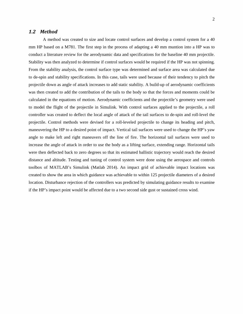
1.2 Method A method was created to size and locate control surfaces and develop a control system for a 40
mm HP based on a M781. The first step in the process of adapting a 40 mm muntion into a HP was to
conduct a literature review for the aerodynamic data and specifications for the baseline 40 mm projectile.
Stability was then analyzed to determine if control surfaces would be required if the HP was not spinning.
From the stability analysis, the control surface type was determined and surface area was calculated due
to de-spin and stability specifications. In this case, tails were used because of their tendency to pitch the
projectile down as angle of attack increases to add static stability. A build-up of aerodynamic coefficients
was then created to add the contribution of the tails to the body so that the forces and moments could be
calculated in the equations of motion. Aerodynamic coefficients and the projectile’s geometry were used
to model the flight of the projectile in Simulink. With control surfaces applied to the projectile, a roll
controller was created to deflect the local angle of attack of the tail surfaces to de-spin and roll-level the
projectile. Control methods were devised for a roll-leveled projectile to change its heading and pitch,
maneuvering the HP to a desired point of impact. Vertical tail surfaces were used to change the HP’s yaw
angle to make left and right maneuvers off the line of fire. The horizontal tail surfaces were used to
increase the angle of attack in order to use the body as a lifting surface, extending range. Horizontal tails
were then deflected back to zero degrees so that its estimated ballistic trajectory would reach the desired
distance and altitude. Testing and tuning of control system were done using the aerospace and controls
toolbox of MATLAB’s Simulink (Matlab 2014). An impact grid of achievable impact locations was
created to show the area in which guidance was achievable to within 125 projectile diameters of a desired
location. Disturbance rejection of the controllers was predicted by simulating guidance results to examine
if the HP’s impact point would be affected due to a two second side gust or sustained cross wind.
3
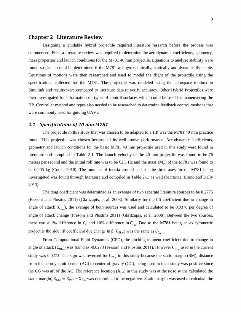
Chapter 2 Literature Review Designing a guidable hybrid projectile required literature research before the process was
commenced. First, a literature review was required to determine the aerodynamic coefficients, geometry,
mass properties and launch conditions for the M781 40 mm projectile. Equations to analyze stability were
found so that it could be determined if the M781 was gyroscopically, statically and dynamically stable.
Equations of motions were then researched and used to model the flight of the projectile using the
specifications collected for the M781. The projectile was modeled using the aerospace toolbox in
Simulink and results were compared to literature data to verify accuracy. Other Hybrid Projectiles were
then investigated for information on types of control surfaces which could be used for maneuvering the
HP. Controller method and types also needed to be researched to determine feedback control methods that
were commonly used for guiding UAVs.
2.1 Specifications of 40 mm M781 The projectile in this study that was chosen to be adapted to a HP was the M781 40 mm practice
round. This projectile was chosen because of its well-known performance. Aerodynamic coefficients,
geometry and launch conditions for the basic M781 40 mm projectile used in this study were found in
literature and compiled in Table 2-1. The launch velocity of the 40 mm projectile was found to be 76
meters per second and the initial roll rate was to be 62.5 Hz and the mass (Mp) of the M781 was found to
be 0.205 kg (Cooke 2010). The moment of inertia around each of the three axes for the M781 being
investigated was found through literature and compiled in Table 2-1, as well (Martinez, Bruno and Kelly
2013).
The drag coefficient was determined as an average of two separate literature sources to be 0.2775
(Fresoni and Plostins 2011) (Gkritzapis, et al. 2008). Similarly for the lift coefficient due to change in
angle of attack (𝐶𝐿𝛼), the average of both sources was used and calculated to be 0.0378 per degree of
angle of attack change (Fresoni and Plostins 2011) (Gkritzapis, et al. 2008). Between the two sources,
there was a 1% difference in 𝐶𝐷 and 10% difference in 𝐶𝐿𝛼. Due to the M781 being an axisymmetric
projectile the side lift coefficient due change in β (𝐶𝑆𝐿𝛽) was the same as 𝐶𝐿𝛼.
From Computational Fluid Dynamics (CFD), the pitching moment coefficient due to change in
angle of attack (Cmα) was found as -0.0273 (Fresoni and Plostins 2011). However Cmα used in the current
study was 0.0273. The sign was reversed for Cmα in this study because the static margin (SM), distance
from the aerodynamic center (AC) to center of gravity (CG), being used in their study was positive since
the CG was aft of the AC. The reference location (Xref) in this study was at the nose so the calculated the
static margin, XSM = Xref − XAC was determined to be negaitive. Static margin was used to calculate the

4
pitching moment coefficient as Cmα = CLα(XSM), where the pitching moment was found to be negative.
Due to symmetry of the body the yawing moment coefficient due to the change in β (Cnβ) was also
determined to be -0.0273. Pitch and yaw damping coefficient (𝐶𝑚𝑞 and 𝐶𝑛𝑟, respectively) due to pitch rate
(q) and yaw rate (r) were found to be -0.1 (Dupuis 2007). In (Lyon 1997) the Magnus force coefficient
(𝐶𝑚𝑝𝛼) for the M781 was found to be 0.1325.
Table 2-1: Standard M781 40 mm Practice Round Specifications
Constant Value Source
𝐶𝐷 0.2775 (Fresoni and Plostins 2011),
(Gkritzapis, et al. 2008)
𝐶𝐿𝛼 𝑎𝑛𝑑 𝐶𝑆𝐿𝛽 2.166 (per rad)
0.0378 (per deg.)
(Fresoni and Plostins 2011),
(Gkritzapis, et al. 2008)
𝐶𝑚𝛼𝐶𝐺 𝑎𝑛𝑑 𝐶𝑛𝛽𝐶𝐺
1.564 (per rad)
0.0273 (per deg.) (Fresoni and Plostins 2011)
𝐶𝑚𝑝𝛼
0.1325 (per rad)
0.0023 (per deg.) (Lyon 1997)
𝐶𝑚𝑞 𝑎𝑛𝑑 𝐶𝑛𝑟 -5.73 (per rad)
-0.1 (per deg.) (Dupuis 2007)
𝑑 0.04 m
𝐼𝑥𝑥 5.4412×10⁻⁵ kg m2 (Martinez, Bruno and Kelly 2013)
𝐼𝑦𝑦 𝑎𝑛𝑑 𝐼𝑧𝑧 1.19215×10⁻⁴ kg m2 (Martinez, Bruno and Kelly 2013)
𝑀𝑝 0.205 kg (Cooke 2010)
𝑝 62.5 Hz (Cooke 2010)
𝐴𝑟𝑒𝑓 0.00126 m2
𝑉 76 m/s (Cooke 2010)
𝑋𝐴𝐶 0.0142 m (Martinez, Bruno and Kelly 2013)
𝑋𝐶𝐺 0.0864 m (Dupuis 2007)

5
𝜌 1.2 kg/m3
2.2 Stability Analysis for Spinning and Non-spinning Projectiles Research was conducted to determine if stability of a projectile could be analytically calculated.
Equations were found in (Milinovic, et al. 2012), (Wilson 2007) and (Carlucci and Jacobson 2008) that
used the projectile’s geometry and aerodynamic coefficients to analyze the stability of a non-spinning or
spinning projectile. The stability criterion for a projectile differs depending if the projectile is spinning or
not. A spinning projectile must be gyroscopically and dynamically stable, and if the projectile is not
spinning, it must be statically and dynamically stable. Criteria found in literature were used to estimate
stability of the projectile. Figure 2-1 shows the orientation of the projectile and was necessary in order to
determine the moments of inertia about each axis (Vogel 2012). In Figure 2-1 (Vogel 2012) used the axis
labels 1, 2 and 3 to describe the earth referenced coordinate system, x, y and z, respectively.
Figure 2-1: Body-fixed Coordinate System (Vogel 2012)
The gyroscopic stability criterion (Sg), defined in equation (2-1), was used to calculate if a
projectile would be gyroscopically stable due do its mass properties, motion and aerodynamics. If Sg was
greater than ‘1’ then the projectile was estimated to be gyroscopically stable and unstable if below one
(Milinovic, et al. 2012) (Wilson 2007) (Carlucci and Jacobson 2008). Similar to a spinning top, if the spin
rate is high enough the projectile will remain oriented with the freestream velocity. After looking at
equation (2-1) there is a minimum roll rate (pmin) where Sg falls below ‘1’. The value of pmin could be
considered the minimum roll rate for gyroscopic stability for a particular projectile with known moments
of inertia, aerodynamics and dimensions. This roll rate of the projectile could be adjusted by adding
canted fins to the projectile or changing the rifling in the barrel. A projectile with a constant moment of
inertia about the x-axis (Ixx), moment of inertia about the y-axis (Iy y), reference area (Aref), pitching

6
moment coefficient with respect to CG (CmαCG) and diameter (d) at a specific flight air density (ρ) and
velocity (V) could only have its roll rate (p) adjusted to ensure a projectile was gyroscopically stable.
A projectile may be gyroscopically stable according to the Sg calculated, but it is also important
that the projectile was dynamically stable. Dynamically stable means that the oscillatory motion of the
projectile naturally returning to steady state is properly damped. In (Raymer 1999), the dynamic stability
for an aircraft refers to the balance of inertial and damping forces resisting the change in body angle rates.
The damping forces are aerodynamic forces that are proportional to the pitch, roll and yaw rates (Raymer
1999). A dynamically stable projectile is similar to an overdamped or critically damped mechanical
systems where the pitch, roll and yaw angles oscillate to a steady state equilibrium value. A projectile is
determined to be dynamically stable if the inequality of equation (2-7) was true. Equation (2-7) required
that the dynamic stability criteria (Sd), equation (2-6) and Sg, equation (2-1) be known.
Calculating those two values was done by solving equations (2-2) through (2-5). Where equation
(2-2) was used to solve for the non-dimensional radius of gyration about the x-axis (rx) and equation (2-3)
solves the non-dimensional radius of gyration about the y-axis (ry) (Wilson 2007). In equations (2-4) and
(2-5) the values T and H were used as a non-dimensional terms to consolidate equation (2-6) where CD
was the drag coefficient and Cmq was the pitch damping coefficient. Equation (2-6) was used to calculate
Sd. CLα was the lift coefficient with change in angle of attack and Cmpα was the pitching moment
coefficient due the projectile rolling and being at an angle of attack.
��𝑥 = �
𝐼𝑥𝑥𝑀𝑝𝑑2
(2-2)
��𝑦 = �
𝐼𝑦𝑦𝑀𝑝𝑑2
(2-3)
𝑇 = �𝜌𝐴𝑟𝑒𝑓𝑑3
2𝐼𝑦𝑦� �𝐶𝐿𝛼 + ��𝑥−2𝐶𝑚𝑝𝛼
� (2-4)
𝐻 = �𝜌𝐴𝑟𝑒𝑓𝑑
2𝑀𝑝��𝐶𝐿𝛼 − 𝐶𝐷 − ��𝑦−2𝐶𝑚𝑞� (2-5)
𝑆𝑑 =2𝑇𝐻
(2-6)
1𝑆𝑔
> 𝑆𝑑(2− 𝑆𝑑) (2-7)
𝑆𝑔 =
𝐼𝑥𝑥2 𝑝2
2𝜌𝐼𝑦𝑦𝐴𝑟𝑒𝑓𝑑𝑉2𝐶𝑚𝛼
(2-1)
7
For a spinning projectile, the Magnus force component also causes the projectile to move left or
right off the line of fire, called yaw of repose (𝜉𝑔) (Milinovic, et al. 2012) (Wilson 2007) (Jie, et al.
2013). In equation (2-8), the Magnus direction of drift is estimated due to the sign of the value inside the
parenthesis. If the static stability criterion (M) was much greater than the non-dimensional term (PT) then
the drift in the imaginary, out of axis, direction could be ignored. Where T was defined in equation (2-4)
and P was a non-dimensional roll rate factor, calculated by equation (2-9). Then, if the value inside the
parenthesis was positive, the pitching moment coefficient was negative, then the projectile would tend to
drift left. However, if the value inside the parenthesis was negative, the pitching moment coefficient was
positive, then the projectile would tend to drift right (Wilson 2007).
𝜉𝑔 = �
−𝑃𝑀 + 𝑗𝑃𝑇
�𝑔𝑑𝑉0−2 (2-8)
𝑃 =𝐼𝑥𝑥𝐼𝑦𝑦
𝑝𝑑𝑉
(2-9)
When a projectile is not spinning, there is no gyroscopic stability force to create a restoring
moment for the projectile’s angle of attack. For a non-spinning projectile to be stable, it must be statically
stable and dynamically stable. Being statically stabile means when the projectile was disrupted from its
initial trajectory it will return to its steady state orientation. For the M781 to be statically stable, M of
equation (2-10) must be less than zero. Also, from equation (2-10), it was found that Cmα must be
negative for the projectile to be statically stable since all other variables were constant.
𝑀 = �
𝜌𝐴𝑟𝑒𝑓𝑑3
2𝐼𝑦𝑦�𝐶𝑚𝛼 (2-10)
A non-spinning projectile must also be dynamically stable so that perturbations in flight will not
cause the angle of attack or beta angle to uncontrollably oscillate. The dynamic stability criterion for a
non-spinning projectile must satisfy that equation (2-5) is greater than zero.
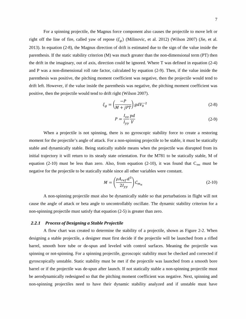
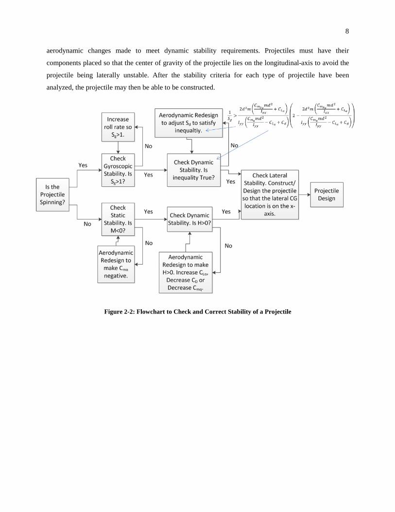
2.2.1 Process of Designing a Stable Projectile A flow chart was created to determine the stability of a projectile, shown as Figure 2-2. When
designing a stable projectile, a designer must first decide if the projectile will be launched from a rifled
barrel, smooth bore tube or de-spun and leveled with control surfaces. Meaning the projectile was
spinning or not-spinning. For a spinning projectile, gyroscopic stability must be checked and corrected if
gyroscopically unstable. Static stability must be met if the projectile was launched from a smooth bore
barrel or if the projectile was de-spun after launch. If not statically stable a non-spinning projectile must
be aerodynamically redesigned so that the pitching moment coefficient was negative. Next, spinning and
non-spinning projectiles need to have their dynamic stability analyzed and if unstable must have
8
aerodynamic changes made to meet dynamic stability requirements. Projectiles must have their
components placed so that the center of gravity of the projectile lies on the longitudinal-axis to avoid the
projectile being laterally unstable. After the stability criteria for each type of projectile have been
analyzed, the projectile may then be able to be constructed.
Figure 2-2: Flowchart to Check and Correct Stability of a Projectile
9
2.3 Modeling Flight using Equations of Motion Predicting the flight of a projectile required a Six Degree of Freedom (6DoF) simulation. A 6DoF
simulation was used to numerically calculate the orientation and position for the projectile. Inside the
simulator equations of motion were used to solve Newton’s second law to balance inertial with external
forces of the projectile. The earth fixed coordinate system used in flight applications was oriented from a
specified ground location with the z-axis normal to the gravity vector, in the direction of gravity (Phillips
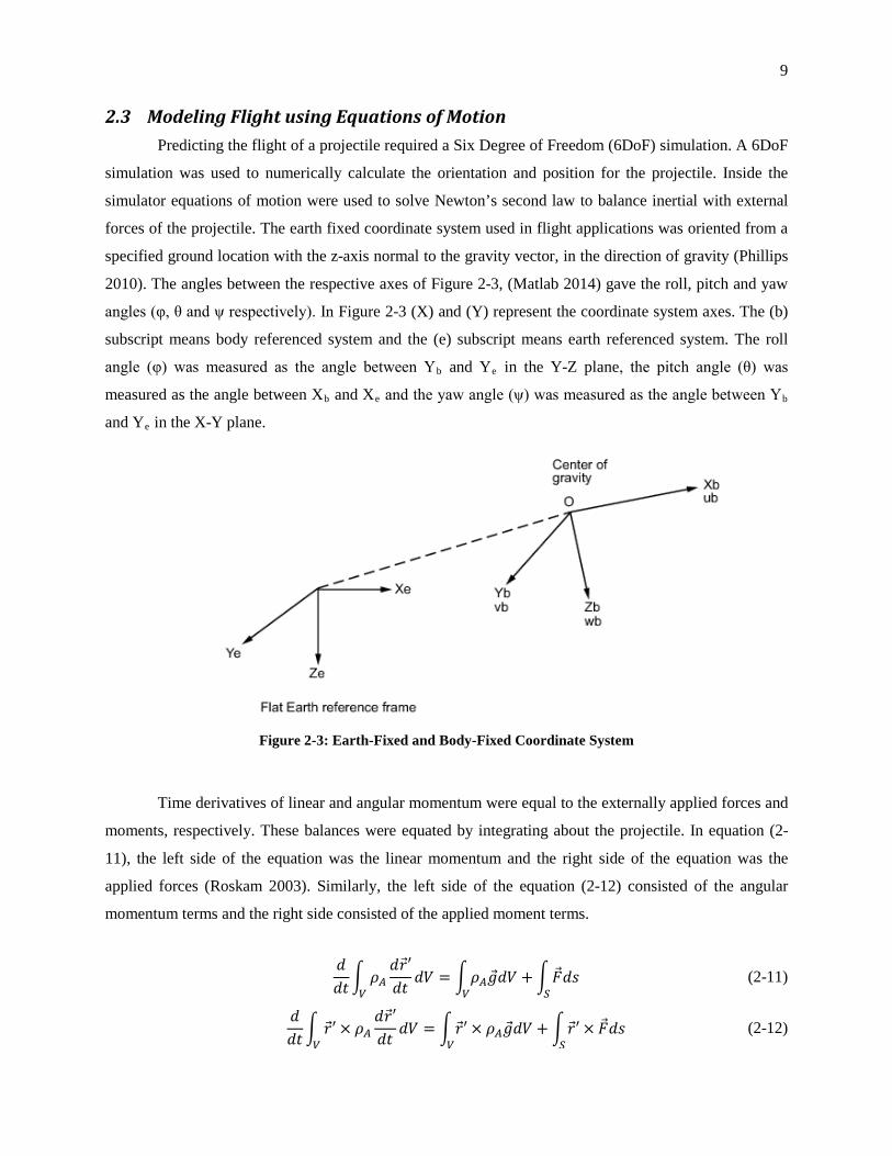
2010). The angles between the respective axes of Figure 2-3, (Matlab 2014) gave the roll, pitch and yaw
angles (φ, θ and ψ respectively). In Figure 2-3 (X) and (Y) represent the coordinate system axes. The (b)
subscript means body referenced system and the (e) subscript means earth referenced system. The roll
angle (φ) was measured as the angle between Yb and Ye in the Y-Z plane, the pitch angle (θ) was
measured as the angle between Xb and Xe and the yaw angle (ψ) was measured as the angle between Yb
and Ye in the X-Y plane.
Figure 2-3: Earth-Fixed and Body-Fixed Coordinate System
Time derivatives of linear and angular momentum were equal to the externally applied forces and
moments, respectively. These balances were equated by integrating about the projectile. In equation (2-
11), the left side of the equation was the linear momentum and the right side of the equation was the
applied forces (Roskam 2003). Similarly, the left side of the equation (2-12) consisted of the angular
momentum terms and the right side consisted of the applied moment terms.
𝑑𝑑𝑡� 𝜌𝐴
𝑑𝑟′𝑑𝑡
𝑑𝑉
𝑉= �𝜌𝐴��𝑑𝑉
𝑉+���𝑑𝑠
𝑆 (2-11)
𝑑𝑑𝑡� 𝑟′ × 𝜌𝐴
𝑑𝑟′𝑑𝑡
𝑑𝑉
𝑉= �𝑟′× 𝜌𝐴��𝑑𝑉
𝑉+ �𝑟′× ��𝑑𝑠
𝑆 (2-12)

10
Where: 𝜌𝐴 𝑤𝑎𝑠 𝑡ℎ𝑒 𝑝𝑟𝑜𝑗𝑒𝑐𝑡𝑖𝑙𝑒 𝑚𝑎𝑠𝑠 𝑑𝑒𝑛𝑠𝑖𝑡𝑦,
So, 𝑚 = ∫ 𝜌𝐴𝑑𝑉 𝑉 ,
And, 𝑑𝑚𝑑𝑡
= 0
Using the integral forms of Newton’s second law in equations (2-11) and (2-12) and the body
orientation of the projectile, the linear momentum and force terms along with the angular momentum and
moment terms could be separated into their three directions and rotations. In equations (2-13) through (2-
15), the earth referenced velocity vector and the orientation were known, and used to compile the linear
force equations (Roskam 2003). The roll, pitch and yaw rate (p, q and r, respectively) were determined
from equations (2-16) through (2-18), (Roskam 2003). Similar to the force equations, angular momentum
and moments of inertia were able to be separated into equations (2-19) through (2-21), (Roskam 2003).
Equations (2-13) through (2-15) and (2-19) through (2-21) were modified to remove forces and moments
due to thrust, since no thrust force was applied for the projectile studied in this case.
𝑀𝑝(�� − 𝑣𝑟 +𝑤𝑞) = −𝑀𝑝𝑔 sin𝜃 + 𝐹𝑥 (2-13)
𝑀𝑝(�� + 𝑢𝑟 − 𝑤𝑝) = 𝑀𝑝𝑔 sin𝜑 cos𝜃 + 𝐹𝑦 (2-14)
𝑀𝑝(�� − 𝑢𝑞 + 𝑣𝑝) = 𝑀𝑝𝑔 cos𝜑 sin𝜃 + 𝐹𝑧 (2-15)
𝑝 = �� − �� sin𝜃 (2-16)
𝑞 = �� cos𝜑 + �� cos𝜃 sin𝜑 (2-17)
𝑟 = �� cos𝜃 cos𝜑 − �� sin𝜑 (2-18)
𝐼𝑥𝑥�� − 𝐼𝑥𝑧�� − 𝐼𝑥𝑧𝑝𝑞 + �𝐼𝑧𝑧 − 𝐼𝑦𝑦�𝑟𝑞 = ℓ (2-19)
𝐼𝑦𝑦�� + (𝐼𝑥𝑥 − 𝐼𝑧𝑧)𝑝𝑟 + 𝐼𝑥𝑧(𝑝2 − 𝑟2) = 𝑚 (2-20)
𝐼𝑧𝑧�� − 𝐼𝑥𝑧�� + �𝐼𝑦𝑦 − 𝐼𝑥𝑥�𝑝𝑞 + 𝐼𝑥𝑧𝑞𝑟 = 𝑛 (2-21)
Equations (2-13) through (2-15) and (2-19) through (2-20) then needed to be modified
individually to determine the linear acceleration in the x, y and z direction (u, v and w respectfully) and
the angular acceleration about the x, y and z axis (p, q and r respectfully). Those equations were
algebraically manipulated so that the linear and angular accelerations could be calculated, using equations
(2-22) through (2-27).
�� =𝐹𝑥𝑀𝑝
− 𝑔 sin𝜃 + 𝑟𝑣 − 𝑞𝑤 (2-22)
�� =
𝐹𝑦𝑀𝑝
+ 𝑔 sin𝜑 cos𝜃 + 𝑝𝑤 − 𝑟𝑢 (2-23)

11
�� =𝐹𝑧𝑀𝑝
+ 𝑔 cos𝜑 cos𝜃 + 𝑞𝑢 − 𝑝𝑣 (2-24)
�� =
ℓ𝐼𝑧𝑧 + 𝑛𝐼𝑥𝑧 + 𝑝𝑞�𝐼𝑥𝑥𝐼𝑥𝑧 − 𝐼𝑦𝑦𝐼𝑥𝑧 + 𝐼𝑧𝑧𝐼𝑥𝑧� + 𝑞𝑟�𝐼𝑦𝑦𝐼𝑧𝑧 − 𝐼𝑥𝑧2 − 𝐼𝑧𝑧2 �𝐼𝑥𝑥𝐼𝑧𝑧 − 𝐼𝑥𝑧2
(2-25)
�� =
𝑚 + 𝑝𝑟(𝐼𝑧𝑧 − 𝐼𝑥𝑥) + (𝑟2 − 𝑝2)𝐼𝑥𝑧𝐼𝑦𝑦
(2-26)
�� =
ℓ𝐼𝑧𝑥 + 𝑛𝐼𝑥𝑥 + 𝑟𝑞�𝐼𝑦𝑦𝐼𝑥𝑧 − 𝐼𝑥𝑥𝐼𝑥𝑧 − 𝐼𝑧𝑧𝐼𝑥𝑧� + 𝑞𝑝�𝐼𝑥𝑥2 − 𝐼𝑥𝑥𝐼𝑦𝑦 + 𝐼𝑥𝑧2 �𝐼𝑥𝑥𝐼𝑧𝑧 − 𝐼𝑥𝑧2
(2-27)
In equations (2-22) through (2-27), initial conditions (mass, g, moments of inertia) were given.
However the three directional forces and moments (Fx, Fy, Fz, ℓ, m and n) were still needed to be
calculated at each time step (Phillips 2010). These forces and moments were calculated by adding up all
the external aerodynamic forces and moments by using an aerodynamic build-up of coefficients.
Coefficients were used to solve for the total external forces and moments on the projectile. The external
forces on the projectile (axial, side and normal forces) were calculated using the transformation in
equations (2-28) through (2-30) and the orientation of the projectile to the freestream shown in Figure
2-4. Where the drag, lift and side lift coefficients (CD, CL and CSL) were known from literature data or
estimated through a build-up of aerodynamic coefficients.
CGAC
CN
CA
CD
CL
V∞
CGAC
V∞
CA
CD
CSLCSF
Side View
Top View
α
β
Figure 2-4: CL, CD and CSL to CN, CA and CY

12
𝐶𝑁 = 𝐶𝐿 𝑐𝑜𝑠(𝛼) + 𝐶𝐷 𝑠𝑖𝑛(𝛼) (2-28)
𝐶𝐴 = −𝐶𝐿 𝑠𝑖𝑛(𝛼) + 𝐶𝐷 𝑐𝑜𝑠(|𝛼| + |𝛽|) − 𝐶𝑆𝐿 𝑠𝑖𝑛(𝛽) (2-29)
𝐶𝑌 = 𝐶𝑆𝐿 𝑐𝑜𝑠(𝛽) + 𝐶𝐷𝑠𝑖𝑛 (𝛽) (2-30)
The total force and moment equations required to solve the equations of motion were compiled as
equations (2-31) through (2-36). Where the rolling, pitching and moment coefficients (Cℓ, Cm and Cn)
were also solved using literature data or an aerodynamic build-up. The pitching and yawing moments
were multiplied by the reference length (ℓref) which was assumed to be 0.1 meters.
𝐹𝑥 = .5𝜌𝐴𝑟𝑒𝑓𝑉2𝐶𝐴 (2-31)
𝐹𝑌 = .5𝜌𝐴𝑟𝑒𝑓𝑉2𝐶𝑌 (2-32)
𝐹𝑍 = .5𝜌𝐴𝑟𝑒𝑓𝑉2𝐶𝑁 (2-33)
ℓ = .5𝜌𝐴𝑟𝑒𝑓ℓ𝑟𝑒𝑓𝑉2𝐶ℓ (2-34)
𝑚 = .5𝜌𝐴𝑟𝑒𝑓ℓ𝑟𝑒𝑓𝑉2𝐶𝑚 (2-35)
𝑛 = .5𝜌𝐴𝑟𝑒𝑓ℓ𝑟𝑒𝑓𝑉2𝐶𝑛 (2-36)
2.4 Six Degree of Freedom Simulation of M781 Using the coefficients and specifications found in literature for the M781, equations of motion
were solved using Simulink’s 6DoF simulation. The simulation was used to estimate the trajectory of the
M781 and examine control methods. A projectile flight simulator was used as the base of the model that
will be used to determine the flight characteristics of this projectile (Wilhelm, et al. 2012). The highest
level block of the model is shown in Figure 2-5. The ‘Calc Forces’ block was used to calculate the
aerodynamic coefficients due to the projectile’s orientation (States). These coefficients were then
multiplied by the reference area, dynamic pressure and reference length to be converted to forces and
moments. The equations of motion were then solved using the forces and moments described in Section
2.3. The 6DoF simulation then determined the earth-fixed velocity, earth-fixed position, earth-fixed
orientation, body-fixed orientation, body-fixed velocity, body-fixed angular rate, body-fixed angular
acceleration and body-fixed accelerations for the M781.

13
Figure 2-5: Simulation Model
2.4.1 M781 Model Verification
The 6DoF model that was constructed for this work was verified for accuracy by matching its
simulation results with two different cases for the M781. The cases that the model was compared against
were literature data for maximum range and literature simulation results for the M781. Using the
coefficients and initial conditions compiled in Table 2-1 the M781 was simulated and compared with
results from literature.
In multiple literature sources the maximum range for the M781 40 mm projectile was found to be
400 meters when landing at the same altitude that it was launched (Cooke 2010) (MLM International
2005) (ALS Technologies 2009). However, in these literature sources the launch elevation angle was not
given for the maximum range condition. So the launch angle that yielded the farthest range was
determined by simulating all launch angles with the specifications found in Table 2-1. From Figure 2-6
the launch angle for the maximum range condition was found to be 42 degrees. This launch angle was
then simulated and its trajectory was shown in Figure 2-7. Maximum range for the simulated M781 was
found to be 408.1 meters. Meaning the range found using this 6DoF simulation was 2% different than
maximum range of 400 meters found in literature for the M781.

14
Figure 2-6: Simulation to Determine Max Range Launch Angle for M781
Figure 2-7: M781 Trajectory for 42 Deg. Launch Angle
The trajectory for the M781 from the 6DoF model was also compared with simulation results in
(Gkritzapis, et al. 2008). Figure 2-8 shows the simulation results from their simulation for launch angle of
14.7, 30 and 40 degrees. The model created in this work was used to simulate the trajectories for the same
launch angles, shown as Figure 2-9. Results from the two simulations are compared for the two sets of
trajectories in Table 2-2. In Table 2-2 the results of each set of simulations were compiled and it was
shown that each set of simulation results varied by a maximum of 0.21% in final distance and apex
altitude.
10 20 30 40 50 60150
200
250
300
350
400
450
Launch Angle (Degrees)
Ran
ge (M
eter
s)
0 50 100 150 200 250 300 350 4000
20
40
60
80
100
Downrange Distance (Meters)
Alti
tude
(Met
ers)

15
Figure 2-8: Flight Path trajectories for 40 mm projectile from (Gkritzapis, et al. 2008)
Figure 2-9: Flight Path Trajectories from Created Model
Table 2-2: Maximum Range and Altitude from Simulation and Literature Results
Source (Gkritzapis, et al. 2008) Model created in this Study Percent Difference
Distance (m) Altitude(m) Distance(m) Altitude(m) Distance(m) Altitude(m)
14.7 degrees 235 16.7 234.86 16.74 0.05% 0.2%
30 degrees 367 60.5 367.13 60.57 0.04% 0.1%
40 degrees 398 97.0 397.17 96.90 0.21% 0.1%
0 50 100 150 200 250 300 350 4000
10
20
30
40
50
60
70
80
90
100
Downrange Distance (Meters)
Alti
tude
(Met
ers)
14.7 deg. launch angle30 deg. launch angle40 deg. launch angle
16
Results from these simulations show that the model accurately predicts the flight of the M781
compared to other literature sources. Also, the coefficients found in literature were accurate for the
projectile and continued to be used as the coefficients of body during the HP build-up. A control system
of surfaces and a controller could now be added to the model and as long as the control model was
meticulously designed then the model should remain accurate.
2.5 Investigate other HP’s for Control System Methods Three different hybrid projectile designs were investigated to evaluate modifications that were
made to adapt a standard projectile to a HP. The upgrades investigated were added to the projectiles to
increase range and add guidance capabilities. Altercations include control surfaces and controllers added
to maneuver the HPs. All three of the literature designs used a symmetric spin-stabilized projectile,
similar to the M781, which remained spinning during flight.
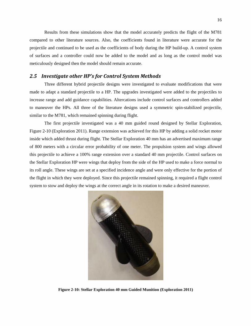
The first projectile investigated was a 40 mm guided round designed by Stellar Exploration,
Figure 2-10 (Exploration 2011). Range extension was achieved for this HP by adding a solid rocket motor
inside which added thrust during flight. The Stellar Exploration 40 mm has an advertised maximum range
of 800 meters with a circular error probability of one meter. The propulsion system and wings allowed
this projectile to achieve a 100% range extension over a standard 40 mm projectile. Control surfaces on
the Stellar Exploration HP were wings that deploy from the side of the HP used to make a force normal to
its roll angle. These wings are set at a specified incidence angle and were only effective for the portion of
the flight in which they were deployed. Since this projectile remained spinning, it required a flight control
system to stow and deploy the wings at the correct angle in its rotation to make a desired maneuver.
Figure 2-10: Stellar Exploration 40 mm Guided Munition (Exploration 2011)

17
DARPA also modified a standard 40 mm munition to a HP called the scorpion, in Figure 2-11
(Lovas, et al. 2009). The Scorpion used synthetic jet actuator as its control surface for maneuvering. The
synthetic jet actuator was used to keep the projectile on course (McMichael, et al. 2004). This projectile
had guidance capability only to be held on its ballistic trajectory because flow control was only used to
correct the Magnus drift of the projectile. This control type was used to reduce drift to its desired impact
location, increasing accuracy.
Figure 2-11: DARPA Scorpion (Lovas, et al. 2009)
The final design examined was a 155 mm round where the baseline projectile, a Howletzer, was
modified with a rotating puck used as a control surface, Figure 2-12 (Fresconi, et al. 2011). This puck was
able to add 700 meters of control authority for the 22,000 meter flight of their specific 155 mm projectile
(Fresconi, et al. 2011). If this control authority ratio was applied to a 40 mm projectile range of 400
meters, there would be 12 meters of control authority. Since there was only one control surface, heading
and longitudinal control were coupled and control authority was measured in range extension and side
movement combined.

18
Figure 2-12: 155mm Puck Control Projectile (Fresconi, et al. 2011)
The previously designed guidable projectiles found in literature remained spinning while being
controlled. First, spinning projectiles have a Magnus force that must be counteracted as well as a yaw of
repose component which pulls them off their original line of fire (Fresconi, et al. 2011) (Wilson 2007).
Second, a spinning projectile would require that the control surfaces only be used at a specific roll angle,
reducing total control authority. Finally, since the body remained spinning the control surfaces could not
hold the projectile at a constant positive angle of attack.
2.6 Control Methods for Aircraft Guidance Aircraft autopilot control methods were investigated to create basic knowledge of concepts that
could be modified for a HP. Traditional manned aircraft and UAV’s have autopilot systems to achieve
specific guidance goals of the aircraft. Autopilots are used to do tasks from altitude holding, velocity
holding, heading tracking and many others. The methods that were used for the HP being adapted in
thesis were heading tracking and altitude holding. However, these methods would need to be modified to
be useful on a projectile with no main wing, no propulsion and a cruciform tail section.
2.6.1 Heading Control
A roll controller for a manned or unmanned aircraft was used to deflect ailerons (on main wing)
and the rudder (on vertical tail) to create a rolling torque to keep the aircraft wings-level in flight
(Christiansen 2004). When an aircraft is at a roll angle, other than zero, the wing creates a lifting force in
the horizontal direction, causing horizontal movement. Meaning that roll and yaw control for a winged
aircraft must be coupled, known as lateral-directional control (Roskam 2003).

19
In (Christiansen 2004), lateral-direction control was shown as inner and outer loop that was used
to maneuver the aircraft to a desired heading. The outer loop of the lateral-directional controller, shown as
Figure 2-13, was used to create an output of desired roll angle to drive the heading error to zero. In this
case, a controller used to drive the heading error to zero was a proportional, integral and derivative (PID)
controller. This roll angle was used as the input to Figure 2-14, in which a proportional and integral (PI)
controller drove the roll angle error to zero by creating aileron deflections. The ailerons on a manned
aircraft are also used to damp the roll rate created during a roll maneuver as the upper summation path of
Figure 2-14 (Christiansen 2004). Roll damping is necessary so harsh roll maneuvers were not felt by
passengers. In Figure 2-15, rudder deflection is used to cause the aircraft to yaw at particular rate.
Figure 2-13: Outer Lateral Heading Angle Controller (Christiansen 2004)
Figure 2-14: Inner Lateral Roll and Roll Rate Control (Christiansen 2004)
Figure 2-15: Inner Lateral Yaw Rate Controller (Christiansen 2004)

20
The basic control system found, led to an initial design envisioned for the heading controller used
in this work. The HP in this study only has vertical tails for heading maneuvering which act like the
rudder on the aircraft in the example.
2.6.2 Longitudinal Control Longitudinal control of a manned or unmanned aircraft normally contains two separate
controllers. The first, is an altitude controller which uses horizontal tail deflections to change the pitch
angle of the aircraft until it reaches a desired altitude. Second, an airspeed controller that adjusted the
throttle position to increase thrust until the aircraft reaches a desired velocity (Ramezani 2012). The outer
loop of the altitude controller uses a PID controller to drive the altitude error to zero by determining the
desired pitch, Figure 2-16. The inner loop of the altitude controller determines the required elevator
deflection to drive the pitch angle to the desired value, determined in the outer loop. This controller
compensates for roll and limits the pitch rate, Figure 2-17 (Christiansen 2004). The airspeed controller,
Figure 2-17, uses a PID controller the drive the airspeed error to zero by changing throttle position to
reduce or increase thrust.
Figure 2-16: Outer Longitudinal Altitude Controller (Christiansen 2004)
Figure 2-17: Inner Longitudinal Airspeed Controller (Christiansen 2004)

21
Figure 2-18: Inner Longitudinal Airspeed Controller (Christiansen 2004)
The longitudinal control method investigated in this thesis could not use an airspeed controller
since the HP did not have direct means of increasing its velocity after it was launched. There was no
propulsion system on the HP in this study so an altitude hold maneuver was not possible since there was
no way of holding a particular altitude using thrust. If an altitude were to be held its velocity would
continually drop due to drag and the tradeoff of kinetic to potential energy. However, the idea of using
horizontal tail (elevator) deflection for pitch controller was utilized to increase the angle of attack so the
body could produce lift extending range without the PID controller. A different loop configuration needed
to be created for the HP to reach a desired altitude at a desired downrange distance while following a
ballistic trajectory.
2.7 Controllers for Aircraft Application Controllers have been used in different applications for many years. They can be used for HVAC
systems, electrical amplification and aerospace applications, etc. In aerospace applications, there were
many different types of controllers that could be used to achieve the designers desired output. From the
large variety of controllers available, a few were investigated for use in the autopilots of this Hybrid
Projectile.

22
In (Haiyang Chao 2007) control techniques were investigated, including; PID, Neural Network,
Fuzzy Logic, Sliding Mode and H∞ control in autopilots (Haiyang Chao 2007). PID was chosen as the
desired control type because it was simple to use, had three tunable gain values and could be implemented
in small UAV applications (Haiyang Chao 2007). The multiple gain values include; proportional, integral
and derivative gain that can be tuned individually to get a desired output. In this controller, the
proportional gain was used to decrease rise time, decrease steady state error and slightly change settling
time but increase overshoot (Matlab 2014). The integral gain was used to eliminate steady state error but
resulted in an increase of overshoot and settling time (Matlab 2014). The derivative gain was used
decrease overshoot, slightly change rise time and decrease settling time but did not change steady state
error (Matlab 2014). Characteristics of the PID controller were found in Matlab’s introduction to PID
controller design. The other controller types could be used but in this case, for the HP being modified, a
PID controller was able to achieve all the goals that were required.
2.8 Literature Conclusions Through the use of background literature research, a plan was determined to achieve the goal of
adapting a M781 to a HP with the use of simulation. The baseline coefficients and geometry were
collected from literature for the M781 projectile which was used as the body of the HP. Stability
equations were then found that could be used to analyze the stability of the projectile by knowing its
geometry and aerodynamic. Equations of motion were then found to be used to predict the flight of the
HP. Forces and moments due to aerodynamics and gravity were required to solve the equations of motion
that could be estimated due to an aerodynamic coefficient build-up. Simulink’s aerospace toolbox was
used to build a model for the HP to apply controllers and predict performance of guidance capabilities.
Current HPs were then investigated for information on types of control surfaces and methods to achieve
guidance. Control methods were researched for aircraft since the HP acted like a UAV while in the
guidance portion of its flight. Types of controllers were then found so advantages and disadvantages
could be compared. It was chosen that PID control be used since it had multiple gain values that could be
used to fine tune guidance performance. This key information was used to create an idea that would be
implemented throughout this thesis.

23
Chapter 3 Control and Stability for a 40 mm HP
3.1 Stability Analysis for the M781 When adapting a M781 to a HP it was necessary to determine if the M781 was stable, so that the
projectile does not tumble and become uncontrollable. First, stability was analytically estimated for the
M781 while spinning then estimated if the M781 was not spinning. After analyzing equation (2-1) for a
standard spinning M781 40 mm round, the gyroscopic stability factor (Sg) was calculated to be 3.51 using
the values compiled in Table 2-1, meaning this projectile was gyroscopically stable. Solving the
inequality for the projectile with the values in Table 2-1, it was estimated that the M781 was dynamically
stable since equation (2-7) was true. Calculations for gyroscopic and dynamic stability are provided in
Appendix A.
However, in this study the HP being adapted was desired to be non-spinning so that the projectile
could be held at an increased angle of attack and the body could be used as a lifting surface. In Appendix
A, the static stability was also analyzed for a standard M781 projectile to determine if it was stable when
not-spinning. It was calculated that the M781 was statically unstable because its CG was aft of the AC,
therefore some type of control surface must be added to make it statically stable.
3.2 Adaptations Required for Stability of M781 to a 40 mm HP The M781 required modification by adding tails to the projectile to transform into a HP so that it
would be statically stable. Tail surfaces were chosen due to their tendency to increase static stability,
pitching the nose down as angle of attack increases. These tail surfaces could also be utilized as control
surfaces, if actuated, to maneuver the HP. The contribution of tails to the projectile was estimated due to a
build-up of aerodynamic coefficients so that the HP’s forces and moments could be calculated. The forces
and moments were calculated using equations (2-31) through (2-36) so that the equations of motion could
be solved for the HP. This meant that the total force and moment coefficients were required for the
projectile body with the contribution of the tail surfaces. Using a coefficient build-up also allowed for
multiple tail geometries to be considered. By changing the span, chord and location of the tails, the values
of the aerodynamic coefficients changed. These coefficients were calculated for multiple tail geometries
to determine which tail sizing ensured that stability was achieved according to the stability requirements
in Section 2.2.

24
3.2.1 Aerodynamic Coefficients Contribution of Tail Surfaces Adding tails to a projectile changes the aerodynamic forces and moments, and in turn changes its
flight. These changes were accounted for by adding the coefficient contribution of the tails. The added
aerodynamic coefficients from the tail were then used to estimate the behavior of the actual projectile.
The vertical and horizontal tails deflect positive and negative with respect to the freestream velocity as
shown in Figure 3-1, as δVT and δHT. In Figure 3-1 the tail deflections are shown in their positive direction
with respect to the freestream. The coefficient build-up begins from the coefficients for the M781 with the
added effect of the tails. The M781 coefficients from Table 2-1 were denoted in the coefficient build-up
with a (Body) subscript.
β
δVT
δHT
α
Velocity
Velocity
Figure 3-1: Tail Deflections With Respect to Freestream Velocity
3.2.1.1 Drag
The total drag of the projectile was determined by adding the drag contribution from the tails to
the contribution from the projectile’s body. The total drag force was determined by adding the drag
coefficient of the body from Table 2-1 to the additional coefficient values determined for the designed tail
surfaces. It was assumed that the tail surfaces used were flat plates. The drag of the tail was comprised of
its zero lift drag (𝐶𝐷0𝑇𝑎𝑖𝑙) as well as induced drag (𝐶𝐷𝑖𝑇𝑎𝑖𝑙 ). The zero lift drag was calculated by using the
skin friction drag of a turbulent flat plate, equation (3-1), as given by Prandtl and found in (White 2006).
The turbulent value was used since the Reynolds number of the tails were in the turbulent range. The lift
induced drag by the tails caused an increased drag coefficient due to the magnitude of deflection from the
freestream velocity. The tail deflection magnitudes were shown in Figure 3-1 and were 𝛼 − 𝛿𝐻𝑇 for the
horizontal tails and 𝛽 + 𝛿𝑉𝑇 for the vertical tails. In equation (3-2), the tail deflection made by the roll
controller (δ) must be multiplied by two since 𝐶𝐿𝛿𝐻𝑇 was calculated for two tails and four tails were

25
defected for de-spin and roll-leveling control. The drag coefficient build-up of equation (3-3) included a
value “2” before the number of tails (N) which stands for the two sides of a flat plate (White 2006).
𝐶𝐷0𝑇𝑎𝑖𝑙 =
0.058
𝑅𝑒𝐿15� (3-1)
𝐶𝐷𝑖𝑇𝑎𝑖𝑙 =
�𝐶𝐿𝛿𝐻𝑇(|𝛼 + 𝛿𝐻𝑇| + |𝛽 − 𝛿𝑉𝑇| + 2|𝛿|)�2
𝜋𝑒𝐴𝑅
(3-2)
𝐶𝐷𝑇𝑜𝑡𝑎𝑙 = 𝐶𝐷𝐵𝑜𝑑𝑦 + 𝐶𝐷0𝑇𝑎𝑖𝑙 �2𝑁𝐴𝑡𝑎𝑖𝑙𝐴𝑟𝑒𝑓
�+ 𝐶𝐷𝑖𝑇𝑎𝑖𝑙𝑁𝐴𝑇𝑎𝑖𝑙𝐴𝑟𝑒𝑓
(3-3)
3.2.1.2 Lift The lift additions due to the tail surfaces were determined next. The lift coefficients at zero
degrees angle of attack and with change in tail deflection were examined. The lift of the tail with zero
degrees of tail deflection was (𝐶𝐿𝑜𝑇𝑎𝑖𝑙 = 0.0) since the tail surfaces were assumed as flat plates, with no
camber. The lift coefficient of the tail with tail deflection was given by equation (3-4), which takes into
account the aspect ratio (ARTail) of the tail surfaces, as given by Prandtl lifting-line theory. There was also
a contribution of lift coefficient due to rate of angle of attack change from the horizontal tails in equation
(3-5), (Roskam 1971). In equation (3-5) the tail efficiency (η) used was assumed to 90% due to the tails
being in the wake of the body while it was being used as a lifting surface. The build-up of the total lift
coefficient, equation (3-6), was compiled using a similar set-up as in (Phillips 2010). In equation (3-6) the
tail deflection magnitude lift coefficient was based on 𝛼 − 𝛿𝐻𝑇 , as seen in Figure 3-1.
𝐶𝐿𝛿𝐻𝑇 =2𝜋
�1 + � 2𝐴𝑅𝑇𝑎𝑖𝑙
��
(3-4)
𝐶𝐿��𝐻𝑇 = 2𝜂𝐶𝐿𝛿𝐻𝑇 (3-5)
𝐶𝐿𝑇𝑜𝑡𝑎𝑙 = 𝐶𝐿𝛼𝐵𝑜𝑑𝑦𝛼 + 𝐶𝐿𝛿𝐻𝑇(𝛼 − 𝛿𝐻𝑇)𝑁𝐴𝑇𝑎𝑖𝑙2𝐴𝑟𝑒𝑓
+ 𝐶𝐿��𝐻𝑇 ���𝑑2𝑉�𝑁𝐴𝑇𝑎𝑖𝑙2𝐴𝑟𝑒𝑓
(3-6)

26
3.2.1.3 Pitching Moment The pitching moment effects introduced by adding tails were created by the projectile spinning
and the tail surfaces having an effective angle of attack. The pitching moment due to the tails being
deflected (𝐶𝑚𝛿𝐻𝑇), equation (3-7), was determined from the flat plate lift coefficient. The pitching
moment due to the roll rate of the projectile (𝐶𝑚𝑝𝑇𝑎𝑖𝑙), equation (3-8), was added because of the recovery
moment created to drive the projectile to zero degrees angle of attack. In the build-up of the pitching
moment coefficient, equation (3-11), 𝐶𝑚𝑝𝑇𝑎𝑖𝑙 was multiplied by the sign of the angle of attack because of
its tendency to pitch down with a positive angle of attack and pitch up with a negative angle of attack.
Equation (3-9) was used to estimate the pitch damping moment coefficient contribution from the
horizontal tail surfaces (𝐶𝑚𝑞𝐻𝑇). The horizontal tail contribution to pitching moment due to the rate of
change in angle of attack (𝐶𝑚��𝐻𝑇) was shown as equation (3-10). The total pitching moment (𝐶𝑚𝑇𝑜𝑡𝑎𝑙)
coefficient was built up as equation (3-11).
𝐶𝑚𝛿𝐻𝑇 =−𝜂2𝜋
�1 + � 2𝐴𝑅𝑇𝑎𝑖𝑙
��
(3-7)
𝐶𝑚𝑝𝑇𝑎𝑖𝑙=−(.6𝜂𝑁𝐴𝑡𝑎𝑖𝑙𝑙𝑡3)
𝐴𝑟𝑒𝑓𝑑�𝑝2
𝑉2� (3-8)
𝐶𝑚𝑞𝐻𝑇= −2.2𝜂𝐶𝐿𝛿𝐻𝑇 �
𝜋180
� (3-9)
𝐶𝑚��𝐻𝑇= −2𝜂𝐶𝐿𝛿𝐻𝑇 �
𝜋180
� (3-10)
𝐶𝑚𝑇𝑜𝑡𝑎𝑙 = 𝐶𝑚𝛼 𝐵𝑜𝑑𝑦(𝛼) + 𝐶𝑚𝛿𝐻𝑇 �
(𝛼 − 𝛿𝐻𝑇)𝜋180
��𝑙𝑡𝑎𝑖𝑙𝑙𝑟𝑒𝑓
� �𝑁𝐴𝑇𝑎𝑖𝑙𝑠2𝐴𝑟𝑒𝑓
� + 𝐶𝑚𝑝𝑡𝑎𝑖𝑙�𝑠𝑖𝑔𝑛(𝛼)�
+ �𝐶𝑚𝑞𝐻𝑇+ 𝐶𝑚𝑞 𝐵𝑜𝑑𝑦��
�180𝜋 � 𝑞𝑑2𝑉
�𝑁𝐴𝑇𝑎𝑖𝑙2𝐴𝑟𝑒𝑓
�𝑙𝑡𝑎𝑖𝑙𝑙𝑟𝑒𝑓
�2
+ 𝐶𝑚��𝐻𝑇���𝑑2𝑉�𝑁𝐴𝑇𝑎𝑖𝑙2𝐴𝑟𝑒𝑓
�𝑙𝑡𝑎𝑖𝑙𝑙𝑟𝑒𝑓
�2
(3-11)

27
3.2.1.4 Side Force The side lift force refers to the force in the y-direction, which is similar to lift in the z-direction.
The side lift force coefficient used the same build up components as lift because the munition was axi-
symmetric. In equation (3-12) the side lift force coefficient from vertical tail deflection (𝐶𝑆𝐿𝛿𝑉𝑇) was the
same as equation (3-4) because the horizontal and vertical tails being used have the same geometry. The
deflection magnitude multiplied by the lift coefficient due to tail deflection is 𝛽 + 𝛿𝑉𝑇, which was defined
in Figure 3-1. Equation (3-13) was the side lift force coefficient contribution from the vertical tails due to
the rate of change in beta angle (𝐶𝑆𝐿��𝑉𝑇). The total side lift force coefficient (𝐶𝑆𝐿𝑇𝑜𝑡𝑎𝑙) was combined as
equation (3-14). The only difference to equation (3-14) from equation (3-6) was that the coefficients were
multiplied by β instead of α.
𝐶𝑆𝐿𝛿𝑉𝑇 =2𝜋
�1 + � 2𝐴𝑅𝑇𝑎𝑖𝑙
��
(3-12)
𝐶 𝑆𝐿��𝑉𝑇= 2𝜂𝐶𝐿𝛿𝐻𝑇 (3-13)
𝐶𝑆𝐿 𝑇𝑜𝑡𝑎𝑙 = 𝐶𝑆𝐿𝛽𝐵𝑜𝑑𝑦𝛽 + 𝐶𝑆𝐿𝛿𝑉𝑇(𝛽 + 𝛿𝑉𝑇)𝑁𝐴𝑇𝑎𝑖𝑙2𝐴𝑟𝑒𝑓
+ 𝐶𝑆𝐿��𝑉𝑇��𝑑2𝑉
𝑁𝐴𝑇𝑎𝑖𝑙2𝐴𝑟𝑒𝑓
(3-14)
3.2.1.5 Yawing Moment
Similarly, the pitching and yawing moments were symmetric and shown as equations (3-15)
through (3-19). However, there was a difference in beta angle being used in this build-up and the beta
angle that determined by the 6DoF simulation. This caused the yaw rate to be of opposite sign convention
from the beta angle. The actual yaw rate was reversed in sign to correct this issue.
𝐶𝑛𝛿𝑉𝑇 =−𝜂2𝜋
�1 + � 2𝐴𝑅𝑇𝑎𝑖𝑙
��
(3-15)
𝐶𝑛𝑝𝑇𝑎𝑖𝑙 =−(.6𝜂𝑁𝐴𝑡𝑎𝑖𝑙𝑙𝑡3)
𝐴𝑟𝑒𝑓𝑑�𝑝2
𝑉2� (3-16)
𝐶𝑛𝑟𝑉𝑇 = −2.2𝜂𝐶𝐿 𝑆𝑖𝑑𝑒𝛿𝑉𝑇 �𝜋
180� (3-17)
𝐶𝑛��𝑉𝑇 = −2𝜂𝐶𝐿 𝑆𝑖𝑑𝑒𝛿𝑉𝑇 �𝜋
180� (3-18)

28
𝐶𝑛𝑇𝑜𝑡𝑎𝑙 = 𝐶𝑛𝛽 𝐵𝑜𝑑𝑦(𝛽) + 𝐶𝑛𝛿𝑉𝑇 �
(𝛽 + 𝛿𝑉𝑇)𝜋180
� �𝑙𝑡𝑎𝑖𝑙𝑙𝑟𝑒𝑓
�𝑁𝐴𝑇𝑎𝑖𝑙2𝐴𝑟𝑒𝑓
+ 𝐶𝑛𝑝𝑡𝑎𝑖𝑙�𝑠𝑖𝑔𝑛(𝛽)�
+ �𝐶𝑛𝑟𝑉𝑇 − 𝐶𝑛𝑟 𝐵𝑜𝑑𝑦� ��180𝜋 � 𝑟𝑑2𝑉
�𝑁𝐴𝑇𝑎𝑖𝑙2𝐴𝑟𝑒𝑓
�𝑙𝑡𝑎𝑖𝑙𝑙𝑟𝑒𝑓
�2
+ 𝐶𝑚��𝐻𝑇���𝑑2𝑉�𝑁𝐴𝑇𝑎𝑖𝑙2𝐴𝑟𝑒𝑓
�𝑙𝑡𝑎𝑖𝑙𝑙𝑟𝑒𝑓
�2
(3-19)
3.2.1.6 Rolling Moment
The presence of tails on a spinning projectile caused a rotational drag to reduce the roll rate (p) of
the projectile. Rotational drag was considered when the tail surfaces were non-deflected as well as
deflected. The non-deflected tail rolling damping coefficient (𝐶𝑙𝑝 𝑛𝑜𝑛−𝑑𝑒𝑓𝑙. 𝑡𝑎𝑖𝑙) was shown as equation
(3-20) (Niskanen 2009). In equation (3-20) non-deflected tail roll damping coefficient was calculated
using the root chord (cr), the tip chord (ct) and the span of the tails (s). In equations (3-20) and (3-22) the
moment arm of the tails about the x-axis (rt) was the projectiles diameter plus half the span of a tail. The
deflected tail rolling damping coefficient (𝐶𝑙𝑝𝑑𝑒𝑓𝑙. 𝑡𝑎𝑖𝑙), equation (3-21), was determined by using the lift
coefficient from each tail that caused a torque on the body. The combined effect of the deflected and non-
deflected tails on the rolling moment coefficient was compiled as equation (3-22).
𝐶𝑙𝑝 𝑛𝑜𝑛−𝑑𝑒𝑓𝑙. 𝑡𝑎𝑖𝑙 =−𝑁𝜂 � 2𝜋
√1 −𝑀2�
𝐴𝑟𝑒𝑓𝑑�𝑐𝑟 + 𝑐𝑡
2𝑟𝑡2𝑠 +
𝑐𝑟 + 2𝑐𝑡3
𝑟𝑡𝑠3 +𝑐𝑟 + 3𝑐𝑡
12𝑠3� �
𝑝𝑉� (3-20)
𝐶𝑙𝑝𝑑𝑒𝑓𝑙. 𝑡𝑎𝑖𝑙 =2𝜋𝜂
(1 + (2 𝐴𝑅𝑡𝑎𝑖𝑙))⁄ (3-21)
𝐶𝑙 𝑇𝑜𝑡𝑎𝑙 = 𝐶𝑙𝑝 𝑛𝑜𝑛−𝑑𝑒𝑓𝑙. 𝑡𝑎𝑖𝑙 �𝑝�180 𝜋� �𝑑
2𝑉 �+ 𝐶𝑙𝑝𝑑𝑒𝑓𝑙.𝑡𝑎𝑖𝑙 �𝛿𝜋
180� �
𝑁𝐴𝑡𝑎𝑖𝑙𝐴𝑟𝑒𝑓
� (𝑟𝑡) (3-22)
With the total aerodynamic coefficients calculated the forces and moments were determined. The
equations of motion were then solved using those aerodynamic forces and moments to model the HP.

29
3.3 Verification of 6DoF model of a HP with Tails An experimental projectile was constructed to validate the 6DoF model using the new build-up of
aerodynamic coefficients from the tails. In this case, the aerodynamic coefficients and geometry were
modified for the values from the experimental projectile. The initial conditions shown throughout this
section for the experimental projectile were compiled in Table 3-1; calculated throughout this section, in
Appendix C and in Appendix D. The experimental projectile was designed due to its launch system and to
ensure stability. The experimental projectile was launched using a 1.5” PVC pipe potato gun style
launcher. The fins were designed to be sub-bore so that projectile would fit inside of the pipe to be
launched. The inner diameter of the PVC pipe was 1.71” so the projectile’s diameter was chosen to be
1.68” (42.67 mm), leaving a small gap so that the projectile did not get stuck in the tube. Stability of this
projectile was calculated by first completing a CG analysis and then ensuring that the AC was rearward of
the CG. The envisioned design was shown as Figure 3-2. This projectile was built in three sections; nose,
body and tail, so components could be added inside of the body and accessed from each end. The three
sections were shown by modifying the color of the body section in Figure 3-2. This experimental
projectile was equipped with a Px4 autopilot (PX4 Autopilot n.d.), voltage regulator and batteries so that
its trajectory could be recorded.
Figure 3-2: Full Projectile with Batteries (Front of Body) and Chip (Rear of Body)
The mass of all the components were measured and the approximate CG location of each
component was determined, with the total mass of the projectile being 0.164 kg. The CG location was
either measured by hand or estimated with the use of SolidWork’s measuring tool. The CG distances were
measured from the nose of the projectile. The CG of the test projectile was calculated to be 96 mm aft of
the nose, shown in Appendix C. Meaning that for the projectile to be stable the AC must be greater than
96 mm.

30
An aerodynamic build-up of the normal force coefficient was completed on each component and
used to determine the AC. The normal force coefficient was calculated using a literature build-up of all
components (Barrowman n.d.). Appendix C shows the steps required to determine the normal force
coefficient with change in angle of attack (CNα) and the AC of each component. The total normal force
coefficient was calculated to be CNα = 0.128 and the AC was determined to be 172 mm aft of the nose.
Resulting in a static margin of 76.5 mm meaning that the projectile was stable since the AC was aft of the
CG.
This test projectile was experimentally tested to determine its range. It was launched
pneumatically in a ‘potato gun style’ launcher, shown as Figure 3-3. The launcher had a 1 ½” PVC pipe
barrel and a 2” PVC pipe pressure chamber. The pressure chamber was connected to an air compressor to
the aft end of the pressure chamber and filled. When the red trigger was pulled the air in the pressure
chamber went through the valve into the barrel accelerating the projectile.
Figure 3-3: Launch System Diagram
The Px4 Autopilot was used to track the orientation and position of the projectile. Setup for the
Px4 Autopilot was shown in Appendix D and was used to retrieve the flight data. From the GPS launch
data the projectile was seen to have travelled 144 meters. The top view of the projectiles flight was shown
in Figure 3-4. The GPS data was converted from Latitude and Longitude to meters then zeroed at the
position where the autopilot was turned on using the code from Appendix F.

31
Figure 3-4: Test Projectile Launch, Zeroed from Starting Location
During launch testing the pressure in the chamber was 100 psi which correlated to a launch
velocity of between 40 and 45 m/sec. This correlation of chamber pressure to muzzle was determined
experimentally by testing multiple pressures and determining the launch velocity using a high speed
camera. Inclination of the launcher was set to approximately 30 degrees. Approximate ranges of launch
velocity and inclination were simulated to show an envelope of possible trajectories. The flight model
built in this section was used to simulate the same launch and the results were compared. The initial
conditions and projectile specifications used in both the flight experiment and simulation are compiled in
Table 3-1. Aerodynamic coefficients were calculated in Appendix D. Simulation results in Figure 3-5
show the minimum and maximum range trajectories due to changing the launch velocity and elevation.
After simulating all combinations of launch velocity and inclination from the ranges of values in Table
3-1, the minimum range resulted from the 40 m/sec at 28 degree launch and the maximum range was
from the 45 m/sec at 32 degrees. All other launch angles and velocities fell within that range. When the
average value of launch angle and velocity, 42.5 m/sec at 30 degrees, was simulation the range was 140.2
meters. Due to the lack of exact values for experimental launch velocity and angle the experimental
results were not a good verification of the accuracy of the model. From Figure 3-5 it was noticed that the
range calculated by the model was up to 23 meters (16%) off of the experimental results. With more
accurate launch conditions the range of simulation data could be reduced and the error could be found.
-10 0 10 20 30 40 50 60 70 80 90-140
-120
-100
-80
-60
-40
-20
0Distance From Starting Position
Easting Distance (meters)
Nor
thin
g D
ista
nce
(met
ers)

32
Table 3-1: Simulation Constants for the Experimental Projectile
Launch Velocity [40 – 45] m/sec
Launch Elevation [28 – 32] degrees
mass 0.164 kg
𝑑 0.04267 m
𝑋𝐴𝐶 0.172 m
𝑋𝐶𝐺 0.096 m
𝐼𝑥𝑥 5.36×10⁻⁴ kg m2
𝐼𝑦𝑦 𝑎𝑛𝑑 𝐼𝑧𝑧 6.07144×10⁻⁴ kg m2
𝐶𝐿𝛼 𝑎𝑛𝑑 𝐶𝑆𝐿𝛽 0.128
𝐶𝑚𝛼𝐶𝐺 𝑎𝑛𝑑 𝐶𝑛𝛽𝐶𝐺 -0.098
𝐶𝐷 0.24
𝐶𝑚𝑞 𝑎𝑛𝑑 𝐶𝑛𝑟 -0.1
Figure 3-5: Simulation Results of Experimental Test
After verifying simulation results with the experimental test, the new coefficient build-up in
model was determined to be useable in this case. A tail controller could now be added to the model and as
long as the tail control model was meticulously designed then the model should remain accurate.
0 20 40 60 80 100 120 140 1600
5
10
15
20
25
30
Downrange Distance (Meters)
Alti
tude
(Met
ers)
40m/s at 28deg42.5m/s at 30deg45m/s at 32degExperiment Range

33
3.4 Tail Sizing for Static and Dynamic Stability Now that tail surface contributions have been added to the 6DoF model, the geometry of the tails
could be calculated. The tails on this HP were required to meet two criteria:
1.) The tail area must satisfy static and dynamic stability criteria for the projectile.
2.) The tail surface area must be large enough to ensure that the HP was de-spun to zero degrees
per second in less than 2 seconds, without the tails being deflected.
Static stability for the HP was determined by varying the chord and span of the tails to calculate
the value of M, equation (2-10). In equation (2-10) 𝐶𝑚𝛼 was the variable that could be adjusted by adding
tails to the projectile, the other values remained constant. In Figure 3-6, the pitching moment coefficient
value with respect to tail chord and span was shown. Static stability was established when the pitching
moment coefficient was less than zero. The dark red section fills in the positive pitching moment
coefficients determined from the tail geometry. Therefore the tail geometry must be chosen from a non-
dark-red location.
Figure 3-6: Static Stability Examination with respect to Tail Sizing
Tail Span (meters)
Tail
Cho
rd (m
eter
s)
0 0.01 0.02 0.03 0.04 0.050
0.01
0.02
0.03
0.04
0.05
Pitc
hing
Mom
ent C
oeffi
cien
t
-8
-7
-6
-5
-4
-3
-2
-1
0

34
The projectile must also be dynamically stable, meaning that the non-dimensionalized dynamic
stability factor (H) from equation (2-5) must be positive. A plot similar to the static stability plot was
created to show the H value with respect to the tail sizing. In Figure 3-7, it was noticed that for all tail
sizes investigated the H value was a positive value, meaning any choice in tail geometry from Figure 3-7
yielded a dynamically stable projectile. However, the values get smaller, less dynamically stable, as they
move towards the upper-right corner of the figure. So the tail geometry was chosen from a point on
Figure 3-6 which yielded a negative pitching moment coefficient and as close to the bottom left corner in
Figure 3-7.
Figure 3-7: Dynamic Stability Examination with respect to Tail Sizing
The tail area required to satisfy the criteria of de-spinning in less than two seconds without tail
deflection was determined by calculating the angular acceleration of the projectile due to the presence of
the tails, using equation (3-23). The roll rate was calculated using a discrete time step then used to solve
the rolling acceleration (��) for the next time step. In this equation, the effective angle of attack (𝛼𝑒𝑓𝑓) was
multiplied by lift coefficient created for a tail on all four tails. The effective angle of attack was the angle
created by freestream velocity and the roll rate (p) as seen in Figure 3-8. They were then multiplied by the
moment arm of each tail (rt) which was considered as the mid span point. As angular acceleration in the
roll axis changes the angular velocity over time, the effective angle of attack of the tails decreases thus
reducing the lifting force on the tails. In equation (3-23), the values that could be modified were the span
and the tail area. By varying these two parameters the roll rate was calculated over time until it reached
zero degrees per second. A table of de-spin times for different tail configurations can be seen in Table
3-2. The de-spin time in this table were based on the roll rate going below 0.01 degrees per second. The
Tail Span (meters)
Tail
Cho
rd (m
eter
s)
0 0.01 0.02 0.03 0.04 0.050
0.01
0.02
0.03
0.04
0.05
H v
alue
2
3
4
5
6
7
8x 10⁻⁶

35
de-spin time table shows that the tail requirements for de-spin are, at least, an area of 600 mm2 and a span
of 30 mm.
VROT
ω Roll Rate
VROT
VEffective
V∞
Front View
Top View
ε ef
f
Figure 3-8: Effective Angle of Attack on tails from Roll Rate
�� =τ
Ixx=
−2𝑞�𝐴𝑟𝑒𝑓𝐶𝐿𝛿𝐻𝑇𝛼𝑒𝑓𝑓𝑟𝑡𝐼𝑥𝑥
=
−.5 ρ N Atail V2 rt 2 π 1 + 2
(s2 Atail)⁄�tan−1 p
V rt
(5.4412 × 10⁻⁵)
(3-23)
Table 3-2: De-spin Time Based on Tail Geometry
From Table 3-2, it was seen that many different combinations of tail chord and span will allow
for de-spin time of less than 2 seconds, but the smallest tail size of 600 mm2 was used as the required tail
area for de-spin. The smallest tail area was chosen to reduce the drag contribution from the tails, since
skin friction drag was proportional to the wetted area. The de-spin times from Table 3-2w ere similar to
the values determined by CFD and numerical flight testing for a 40 mm HP design (Vogel 2012).
Span (mm) Chord (mm) Tail Area (mm2) Time (sec)20 20 400 4.4120 25 500 4.1120 30 600 3.9120 35 700 3.7720 40 800 3.6625 20 500 2.5825 25 625 2.3825 30 750 2.2425 35 875 2.1425 40 1000 2.0730 20 600 1.6430 25 750 1.530 30 900 1.430 35 1050 1.3330 40 1200 1.28

36
The tails were not considered to have affected the moment of inertia for the projectile since a
structural design was not yet done. However, the changes that could occur from the change in CG, AC
and Ixx were examined to determine if this assumption would minimally effect de-spin and stability
criteria. From the calculations shown in Appendix B, if carbon fiber tails were used, the CG would be
shifted aft by 4% of the projectiles diameter while the AC was shifted aft 264% of the projectile
diameters. This resulted in a 5% difference in SM when tails were and were not considered to affect CG
allowing mass to be ignored in this case.
In Appendix B, the change in Ixx due to the tails being added to the projectile was considered. The
de-spin time was seen to be increased by 2% of the total flight time due to the increased moment of
inertia. The moment of inertia should be calculated when the actual design is built but was ignored since
mass properties could be manipulated in this theoretical method.
Now, with both requirements met, the tail geometry was determined. From the two above
conditions the tail area must be 600 mm2 so the span must be 30 mm. This means that the chord of the tail
was 20 mm. The tail surfaces were designed as rectangles so the root chord and tip chord were 20 mm.
The tail geometry was chose as four, 20 mm by 30 mm, tails. This tail geometry yields a pitching moment
coefficient value of -0.0266. This geometry, shown on the modified M781 in Figure 3-9, yielded a
statically and dynamically stable projectile.
Figure 3-9: Modified M781 with Four Tails

37
Chapter 4 Tail Control for Guidance Tail control was added to the flight model of the HP with the use of a tail controller sub-system.
The tail controller sub-system, shown in Figure 4-1 as left most block, was used to calculate the required
tail deflections to de-spin, roll-level and guide the HP to a desired point of impact. The tail controller sub-
model had a “states” input that used rotational angle, rotational velocity and translational velocity which
were received from the ‘6DoF (Euler Angles)’ block (right-center). An input of the rolling moment
coefficient was also important in the switch function, shown later, which was received from the ‘Calc
Forces’ block (left-center).
Figure 4-1: Simulation Model with Tail Control
4.1 Tail Feedback Control using Multiple Controllers Figure 4-2 shows the Tail Controller sub-system of Figure 2-5. In this sub-system the tail
deflection outputs were broken down into the deflection required for roll, heading and vertical control
from top to bottom. In Figure 4-2, each set of tail deflections were determined through separate control
methods with a servo delay applied.
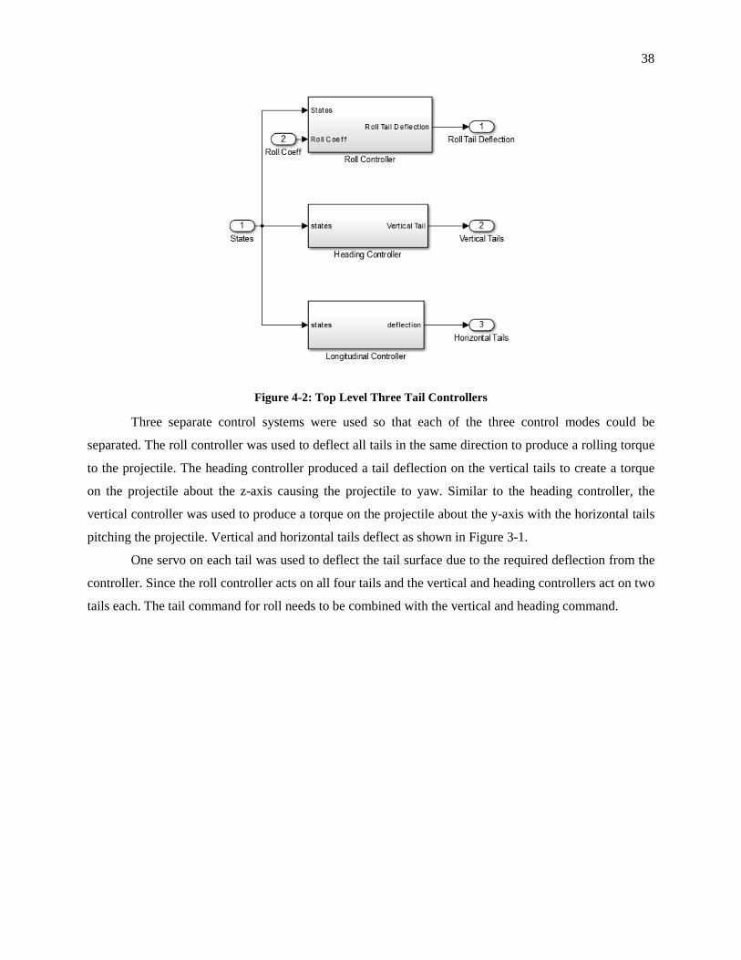
38
Figure 4-2: Top Level Three Tail Controllers
Three separate control systems were used so that each of the three control modes could be
separated. The roll controller was used to deflect all tails in the same direction to produce a rolling torque
to the projectile. The heading controller produced a tail deflection on the vertical tails to create a torque
on the projectile about the z-axis causing the projectile to yaw. Similar to the heading controller, the
vertical controller was used to produce a torque on the projectile about the y-axis with the horizontal tails
pitching the projectile. Vertical and horizontal tails deflect as shown in Figure 3-1.
One servo on each tail was used to deflect the tail surface due to the required deflection from the
controller. Since the roll controller acts on all four tails and the vertical and heading controllers act on two
tails each. The tail command for roll needs to be combined with the vertical and heading command.

39
1
3
4
2
Figure 4-3: Tail Numbering Convention
Figure 4-4: Controller Outputs for Servo Inputs
4.2 Servo Delay Model When using an electric servo, there was a delay from the desired output to the actual angle of the
servo. An electric servo uses an input of a square wave of a particular pulse width that corresponds to a
desired position for the servo arm. The servo arm position could be measured by a change in resistance in
the servo. A transfer function was required to model the delay of the servo to make the simulation model
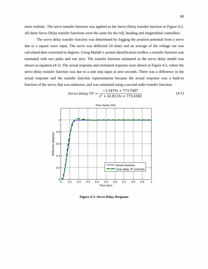
40
more realistic. The servo transfer function was applied as the Servo Delay transfer function in Figure 4-2.
All three Servo Delay transfer functions were the same for the roll, heading and longitudinal controllers.
The servo delay transfer function was determined by logging the position potential from a servo
due to a square wave input. The servo was deflected 24 times and an average of the voltage out was
calculated then converted to degrees. Using Matlab’s system identification toolbox a transfer function was
estimated with two poles and one zero. The transfer function estimated as the servo delay model was
shown as equation (4-1). The actual response and estimated response were shown in Figure 4-5, where the
servo delay transfer function was due to a unit step input at zero seconds. There was a difference in the
actual response and the transfer function representation because the actual response was a built-in
function of the servo, that was unknown, and was estimated using a second order transfer function.
𝑆𝑒𝑟𝑣𝑜 𝐷𝑒𝑙𝑎𝑦 𝑇𝐹 =−1.3479𝑠 + 773.7087
𝑠2 + 42.8113𝑠 + 773.4382 (4-1)
Figure 4-5: Servo Delay Response
0 0.1 0.2 0.3 0.4 0.5 0.6 0.7 0.8 0.9 10
0.2
0.4
0.6
0.8
1
Time (sec)
Def
lect
ion
(deg
rees
)
Time Series Plot:
actual responseservo delay TF estimate

41
4.3 Roll Control The tail controller sub-model, Figure 4-2, was created to make the required tail deflections to de-
spin and roll-level the projectile. It was determined that two separate controllers would be required to de-
spin and roll-level the projectile, and then a transition between these two controllers was needed. The roll
rate (de-spin) controller was designed by having a PID controller that drives the roll rate to zero degrees
per second. The roll position (roll-leveling) controller was designed as a PID controller that drives the
absolute roll position to zero degrees. A PID controller was used because of the combined effects of
having a proportional, derivative and integral controller found in Matlab/Simulink product help (Matlab
2014), as seen in Section 2.7. The PID controller was found in the “Continuous” sub-tab of the
“Simulink” tab in the Simulink Library Browser. Each PID controller runs at a continuous-time domain
with a filter coefficient (N) of N=100.
Each of the four tails had an adjustable local angle of attack that was used to create a normal
force, which caused a rolling torque on the projectile. The tail deflections were limited to 10 degrees in
each direction so that flow separation was not considered. The 10 degree limit of tail deflection was
achieved in the model through the PID advanced tab of the PID controller with a 10 degree and -10
degree saturation limit. A de-spin switch function and controller switch was used to switch between to
two controllers. Tuning of the PID’s and determining the switch function were very critical and are
explained later. A tenth of a second delay was used to allow for tube perturbations to be damped out and
give time for tail surfaces to be deployed.
Figure 4-6 was the roll controller sub-model that had inputs of rotation angles (rot), rotation rates
(omega) and earth referenced velocity (Ve). In Figure 4-6 the upper path was the roll-leveling PID
controller, the middle path was the roll rate controller and the lower path was used for the switch function.
The controller switch chooses the controller in which the actual tail deflection comes from, due to the de-
spin switch function.

42
Figure 4-6: Roll Controller Sub-model
4.3.1 Tuning Dual Mode Roll Controller
The method that was used to tune these PID controllers of the roll control system was a trial and
error technique where all gain values were initially set to zero. One gain value was changed at a time by
running multiple values for that particular gain and analyzing the responses. Once that gain value was
determined it was saved and then the next gain value was evaluated. The time of flight was shown as the
percentage of flight time because different projectiles, with a different total flight time, could use the
same method to be de-spun and roll-leveled.
The first gain value that was determined was the proportional gain for the de-spin controller. The
gain value for the de-spin controller was determined by disconnecting the position controller from the
controller switch block and having the initial roll rate set at 62.5 Hz (Cooke 2010). The gain value was
tuned by determining which gain value gave the quickest roll rate error reduction. The quickest roll rate
error response was chosen as proll= 0.0025 because after testing two gain values the response of roll rate
error goes to zero degrees per second quickest. The roll rate error was seen in Figure 4-7, where
proll=0.0025 yielded the fastest settling time. The roll rate error goes to zero degrees per second and had
no steady state error, so no integral gain was needed for this controller. Also, the derivative gain value
was set at zero since there was no overshoot criterion and the positioning controller takes over when the
roll rate was in a range closer to zero degrees per second.

43
Figure 4-7: Roll Rate Error with Changing Proportional Gain
The gain values that were used in the roll position controller were determined by starting with the
projectile at 180 degrees off the roll-level position and no rotational rate. The roll-leveling controller,
which was disconnected from the controller switch block for the roll rate controller gain value test, must
be reconnected to the controller switch for tail deflection, shown in Figure 4-6. An iterative process was
used since more than one gain value needed to be tuned. A proportional gain of 0.01 was assumed first to
begin the process. The desired response to the roll angle error plot shown in Figure 4-8 is the fastest first
order response.
0% 5% 10% 15%
-2
-1.5
-1
-0.5
0x 104
Percentage of Flight Time
Rol
l Rat
e E
rror (
degr
ees/
seco
nd)
proll=.0025
proll=.01
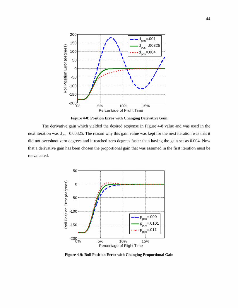
44
Figure 4-8: Position Error with Changing Derivative Gain
The derivative gain which yielded the desired response in Figure 4-8 value and was used in the
next iteration was dpos= 0.00325. The reason why this gain value was kept for the next iteration was that it
did not overshoot zero degrees and it reached zero degrees faster than having the gain set as 0.004. Now
that a derivative gain has been chosen the proportional gain that was assumed in the first iteration must be
reevaluated.
Figure 4-9: Roll Position Error with Changing Proportional Gain
0% 5% 10% 15%-200
-150
-100
-50
0
50
100
150
200
Percentage of Flight Time
Rol
l Pos
ition
Erro
r (de
gree
s)
dpos=.001
dpos=.00325
dpos=.004
0% 5% 10% 15%-200
-150
-100
-50
0
50
Percentage of Flight Time
Rol
l Pos
ition
Erro
r (de
gree
s)
ppos=.009
ppos=.0101
ppos=.011
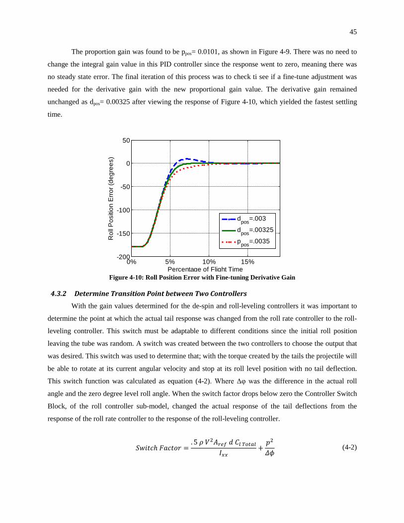
45
The proportion gain was found to be ppos= 0.0101, as shown in Figure 4-9. There was no need to
change the integral gain value in this PID controller since the response went to zero, meaning there was
no steady state error. The final iteration of this process was to check ti see if a fine-tune adjustment was
needed for the derivative gain with the new proportional gain value. The derivative gain remained
unchanged as dpos= 0.00325 after viewing the response of Figure 4-10, which yielded the fastest settling
time.
Figure 4-10: Roll Position Error with Fine-tuning Derivative Gain
4.3.2 Determine Transition Point between Two Controllers
With the gain values determined for the de-spin and roll-leveling controllers it was important to
determine the point at which the actual tail response was changed from the roll rate controller to the roll-
leveling controller. This switch must be adaptable to different conditions since the initial roll position
leaving the tube was random. A switch was created between the two controllers to choose the output that
was desired. This switch was used to determine that; with the torque created by the tails the projectile will
be able to rotate at its current angular velocity and stop at its roll level position with no tail deflection.
This switch function was calculated as equation (4-2). Where Δφ was the difference in the actual roll
angle and the zero degree level roll angle. When the switch factor drops below zero the Controller Switch
Block, of the roll controller sub-model, changed the actual response of the tail deflections from the
response of the roll rate controller to the response of the roll-leveling controller.
𝑆𝑤𝑖𝑡𝑐ℎ 𝐹𝑎𝑐𝑡𝑜𝑟 =
. 5 𝜌 𝑉2𝐴𝑟𝑒𝑓 𝑑 𝐶𝑙 𝑇𝑜𝑡𝑎𝑙𝐼𝑥𝑥
+𝑝2
𝛥𝜙 (4-2)
0% 5% 10% 15%-200
-150
-100
-50
0
50
Percentage of Flight Time
Rol
l Pos
ition
Erro
r (de
gree
s)
dpos=.003
dpos=.00325
ppos=.0035

46
4.3.3 Roll Controller Results In this case for the 40 mm HP the tail geometry was determined to be for 30 mm span by 20 mm
chord. With the tails sized and the dual-mode roll PID feedback loops created, the proportional gain value
was determined for the de-spin controller to be 0.0025. The proportional and derivative gains for the
position controller were determined to be 0.0101 and 0.00325 respectively. The integral and derivative
gain values for the de-spin controller (iroll and droll, respectively) and the integral gain value of the roll
leveling controller (ipos) were set to zero and compiled in Table 4-1. With the transition switch, the 40 mm
HP was de-spun and roll-leveled in 5% of its flight time. The results of the tail geometry as well as the de-
spin and roll-leveling performance was compiled in Table 4-2.
Table 4-1: Compilation of Gain Values from De-spin and Level Controller
Gain Term Gain Value
proll 0.0025
iroll 0.0
droll 0.0
ppos 0.0101
ipos 0.0
dpos 0.00325
Table 4-2: Tail Geometry and Performance Results
Atail 600 mm2
S 30 mm
Cr 20 mm
Ct 20 mm
N 4
De-spin Time 3%
Roll Leveling Time 5%
Results of the roll-leveling controller were shown in Figure 4-11 where the roll angle was
leveling to zero degrees in 5% of the flight time. In Figure 4-11, the roll position never goes above 180
degrees or below -180 degrees because as the projectile rolls past 180 degrees it resets back to -180
degrees. Figure 4-12 shows the results of the de-spin controller where the roll rate decreased to zero
degrees per second in 3% of the flight time.

47
Figure 4-11: Roll Angle through first 20% of Flight
Figure 4-12: Roll Rate through first 20% of Flight
While de-spinning and roll-leveling, the projectiles overall trajectory was minimally changed
from that of the baseline 40 mm M781. Figure 4-13 and Figure 4-14 show the altitude and distance,
respectively, of the flight paths for the M781 projectile and the HP that was configured throughout this
process. From Figure 4-13 it was shown that there was a 3.1% reduction of altitude and in Figure 4-14 a
3.2% reduction in distance was seen, when launched at a 50 degree elevation. The reduction of distance
and altitude were due to the additional drag from the tails. The range and altitude reduction results were
compared with projectile motion equations with drag in Appendix D where the range was seen to be
decreased by 1.9% and the maximum altitude was seen to be reduced by 1.1%.
0% 5% 10% 15%-200
-150
-100
-50
0
50
100
150
200
Percentage of Flight Time
Rol
l Pos
ition
(deg
rees
)
0% 5% 10% 15%-5000
0
5000
10000
15000
20000
Percentage of Flight Time
Rol
l Rat
e (d
egre
es/s
ec)

48
Figure 4-13: X-directional Distance Traveled
Figure 4-14: Z-directional Altitude Traveled
0% 10% 20% 30% 40% 50% 60% 70% 80% 90%100%0%
10%
20%
30%
40%
50%
60%
70%
80%
90%
100%
Percentage of Flight Time
Per
cent
age
of M
axim
um D
ista
nce
Without TailsWith Tails
0% 10% 20% 30% 40% 50% 60% 70% 80% 90%100%0%
10%
20%
30%
40%
50%
60%
70%
80%
90%
100%
Percentage of Flight Time
Per
cent
age
of M
axim
um A
ltitu
de
Without TailsWith Tails

49
4.4 Heading Control After the HP was de-spun and roll leveled it was then desired to be guided to a particular heading
or a specific offset distance from the line-of-fire. Feedback PID control was used as the control method
for vertical tail deflections to control heading. Tuning of the PID controllers was done using the Simulink
Control Design tuning tool.
This tool is found by selecting the “tune” button after the PID controller was opened and the
Function Block Parameters was selected. Tuning was done by adjusting the response time and/or transient
behavior sliders in Figure 4-15, and selecting a slider location that yielded the desired tuned response.
This could not be used for tuning the roll controller because Matlab was not able to linearize the non-
linear equations associated with roll.
Figure 4-15: PID Tuner
The Heading Controller was set up to have two separate choices on how to input the desired
heading. In Figure 4-16 the desired heading angle was an input in which the HP would track to that
desired angle. However, in Figure 4-17, the heading control model allows the actual target location off the
line of fire to be chosen. The inputs were desired distance and desired Y location, where the desire
distance was the downrange distance from launch position and desired y location was the offset from the
line of fire. In this loop, the heading angle required was determined from the difference of actual distance
to required distance and difference in actual Y offset to the desired Y location. The inner loop of the
heading controller drove the yaw rate error to zero, while the outer loop controller drove the heading error

50
to zero. The heading controller was shown in Figure 4-18 in standard feedback form with all connections
labeled.
Figure 4-16: Heading Angle Tracking Sub-model
Figure 4-17: Desired Location Heading Tracking Sub-model

51
Figure 4-18: Inner and Outer Loops of Heading Controller
4.4.1 Filter for yaw rate
The yaw rate response in the simulation required a filter to remove the large magnitude
oscillations created by a maneuver. This was required because the yaw rate controller was not able to
drive error to zero since a tail maneuver would cause yaw rate oscillations many orders of magnitude
higher than the steady yaw rate value from that tail deflection. A first order low pass filter was tested to
see if it would damp the oscillations and yield the required response. In a first order low pass filter the cut
off frequency (ωc) could be manipulated to change the transfer function of the filter. The transfer function
from a filter was shown as equation (4-3).
𝐹𝑖𝑙𝑡𝑒𝑟 𝑇𝐹 =1
12𝜋𝜔𝑐
𝑠 + 1 (4-3)
Multiple cut off frequencies were simulated to see which response most closely resembled the
actual yaw rate response, without the large oscillations. Figure 4-19 shows the original yaw rate response
and three low pass filters which were used to determine the cut off frequency that should be used. In
Figure 4-19 the cut off frequency was varied from 0.15 Hz to 0.25 Hz.

52
Figure 4-19: Yaw Rate for Multiple First Order Filters
Table 4-3: Yaw Rate Response Characteristics from Multiple Cut-off Filters
Data Name Rise Time Peak Time Overshoot %
Original Data 0.0069 sec 1.08 sec 3469%
ωc=.15 0.041 sec 1.13 sec 69%
ωc=.2 0.035 sec 1.13 sec 121%
ωc=.25 0.032 sec 1.13 sec 172%
A cut off frequency of 0.2 Hz was used in a first order cut off filter to damp the oscillations of
yaw rate from vertical tail deflections. 0.2 Hz was chosen as the cut off frequency because it most closely
resembles the response of the original yaw rate response from Table 4-3.
4.4.2 Tuning Heading Controller (Inner and Outer Loop)
The inner loop of the heading controller is the yaw rate controller that controls the vertical tail
deflection to drive the yaw rate error to zero degrees per second. To set up the controller, the P, I, D and
N values were set as a variable so that after tuning was complete the gain values could be saved, Figure
4-20. The tail deflections also have a maximum deflection of 10 degrees in the positive and negative
1 2 3 4 5 6
-10
0
10
20
30
40
50
60
70
Time (sec)
Yaw
Rat
e (d
eg/s
ec)
Original Datawc = .15
wc = .2
wc = .25

53
direction. The tail deflection maximum deflection was set as the saturation limit in the PID Advanced tab
of the PID controller, Figure 4-21.
Tuning and simulation of the PID gain values was done using a zero degree, flat, launch angle
with the gravitation vector as zero magnitude. The other initial conditions described in Table 2-1 were
used as well. This was done so the projectile would not be on a trajectory, but on a level path that it could
be turned from. This assumption could be made since the projectile was at a zero roll angle and the
gravitational force was only in the z-direction.
Figure 4-20: Setting Variables for Gain Values
Figure 4-21: Setting Saturation Limit
The yaw rate desired was the input to the right summing junction, as shown in Figure 4-22, to
tune the inner loop PID controller. In this case the yaw rate desired was chosen to be 5 degrees per
second. A value of 5 degrees per second was chosen because it was a value achievable by tail deflections
within ±10 degrees.
Figure 4-22: Heading Controller with Inputs for Tuning

54
Using the Tune function of the PID controller the yaw rate controller was tuned to have the
smooth first order response by sliding the response time slider to 1.93 seconds, Figure 4-23. In Figure
4-23 the tuned response was based on a unit step function.
Figure 4-23: Initial Yaw Rate Controller Tuning
After the PID gain values were determined by manipulating the slider bars, the projectile was
simulated to see the vertical tail deflection required and if the yaw rate error goes to zero. From Figure
4-24, the PID gain values from the response of Figure 4-23 resulted in the yaw rate error going to zero
while the vertical tail deflections did not oscillate and were within the ±10 degree limit. The PID gain
values in Table 4-4 were used moving forward to the outer loop of the heading controller.

55
Table 4-4: PID Values from Yaw Rate Tune
P_Inner_Heading 0
I_Inner_Heading -.443
D_Inner_Heading 0
N_Inner_Heading 100
Figure 4-24: Yaw Rate Error and Vertical Tail Deflection Response from
PID tune
The outer loop of the Heading controller was used to determine the yaw rate required to get to a
particular heading angle. In this case heading angle error was the input into the PID controller and the
output was the required yaw rate. In the PID controller block there was the ability to change the saturation
limit, similar to the maximum tail deflection in the inner loop PID controller. The saturation limit was
determined by simulating the maximum deflection of 10 degrees. The yaw rate response from the 10
degree tail deflection was used to determine the saturation limit. The response of yaw rate was evaluated
in the Curve Fitting Tool of Matlab to determine that the y intercept was -23.33, Figure 4-25. The y-
intercept was used as the saturation limit because it was the maximum yaw rate achievable without
oscillations. Meaning that ±23.33 was used as the saturation limit.
0 5 10 150
1
2
3
4
5
6
Time (sec)
Yaw
Rat
e E
rror (
deg/
sec)
0 5 10 15-5
-4
-3
-2
-1
0
Time (sec)
Ver
tical
Tai
l Def
lect
ion
(deg
)

56
Figure 4-25: Yaw Rate Response from 10 deg. Vertical Tail Deflection
By choosing a desired heading and connecting the outer loop PID controller with the summation
junction at yaw rate desired the PID slider can be tuned similarly to the inner loop. In Figure 4-26, the
response time slider was chosen as 0.303 seconds because the response to a unit step input was a smooth
response with minimal overshoot and approximately 2.5 second settling time.
Figure 4-26: Initial Heading Angle Control Tune
0 2 4 6 8 10-50
-40
-30
-20
-10
0
Time (sec)
Yaw
Rat
e (d
eg/s
ec)
Yaw Rate DataCurve Fit Data

57
The response from the heading PID tune in Figure 4-26 was simulated to determine if the heading
error went to zero degrees. In Figure 4-27 the heading error went to zero within approximately four
seconds. The PID gain values from the tune of this controller were compiled in Table 4-5.
Table 4-5: PID Values from Heading Tune
P_Outer_Heading 6.7758
I_Outer_Heading 0.8470
D_Outer_Heading 0
N_Outer_Heading 100
Figure 4-27: Heading Error and Yaw Rate Required from PID Tune
When investigating the steady state error by viewing the heading value at 10 seconds it was
noticed that the steady state error was 4×10⁻⁴ degrees. This was not a significant value but was changed
easily by manually adjusting the integral gain value “I_Outer_Heading”. The outer loop integral value
was adjusted to zero and not only was the steady state error removed but the settling time was reduced, as
seen from Figure 4-27 to Figure 4-28. The final PID values from both controllers that were used moving
forward were shown in Table 4-6.
0 2 4 6 8 10-5
0
5
10
15
Time (sec)
Hea
ding
Erro
r (de
g)
0 2 4 6 8 10-10
0
10
20
30
Time (sec)Yaw
Rat
e R
equi
red
(deg
/sec
)

58
Table 4-6: Final Heading Control PID Values
P_Inner_Heading 0
I_Inner_Heading -.443
D_Inner_Heading 0
N_Inner_Heading 100
P_Outer_Heading 6.7758
I_Outer_Heading 0
D_Outer_Heading 0
N_Outer_Heading 100
Figure 4-28: Final Outer Loop PID Tune
4.4.3 Heading Controller Testing
Using the PID values compiled in Table 4-6, the heading tracking was tested by simulating the
projectile at the conditions described in Table 2-1. However, in this simulation the initial roll rate was
zero degrees per second, since the heading control was not used until the HP was roll-leveled. In the first
test, multiple heading angles were evaluated to see if the projectile could track to different heading angles.
From Figure 4-29 the projectile was simulated to track to 10, 30, 50 and 70 degrees. For each required
heading simulation the projectile was able to track to the required heading angle. Figure 4-29 also shows
the vertical tail position required for each simulation.
0 2 4 6 8 10-5
0
5
10
15
Time (sec)
Hea
ding
Erro
r (de
g)
0 2 4 6 8 10-10
0
10
20
30
Time (sec)Yaw
Rat
e R
equi
red
(deg
/sec
)

59
Figure 4-29: Simulation Test of Multiple Heading Angles
In Figure 4-17 there was also a method of tracking the projectile to a specific Y-offset from the
line of fire and downrange distance. Guidance to a desired offset from the line of fire at a specific
downrange distance was tested by simulating two separate impact point cases. In these simulations the
HP’s altitude was not controlled yet, so the projectile crossed through the desired location but may not
land there. Figure 4-30 shows the simulation results for the Y-offset controller of the target locations of
Table 4-7. From these simulations it was seen that the Y-offset controller could be used to accurately
guide a simulated projectile to a desired Y-offset location at a specified distance. Distance from projectile
to target, as it passes through the desired distance, were also shown as the offset in Table 4-7.
Table 4-7: Desired Target Locations for Y-Offset Control
Simulation 1 Simulation 2
Desired Downrange Distance 75% of Max.
Unguided Range
87.5% of Max.
Unguided Range
Desired Y-Offset Distance 1250 Projectile 2500 Projectile
0 1 2 3 4 5 6 7 8 9-20
0
20
40
60
80
Time (sec)
Hea
ding
(deg
)
0 1 2 3 4 5 6 7 8 9-12
-10
-8
-6
-4
-2
0
Time (sec)
Ver
tical
Tai
l Def
lect
ion
(deg
)
10 degrees30 degrees50 degrees70 degrees

60
Diameters Right Diameters Left
Offset from Desired Target 0.7 meters 1.4 meters
Figure 4-30: Desired Y Offset Simulation Tests
4.5 Longitudinal Control The longitudinal controller sub-model of the tail controller model in Figure 4-2 was shown as
Figure 4-31. The longitudinal controller used the states as an input for the HP’s current position, velocity
and pitch angle. This controller was used to determine the horizontal tail deflections required for the HP
to be on its maximum range trajectory, and then used its current states to estimate its ballistic trajectory
Its tails were then deflected back to zero when the estimated trajectory reached the desired impact point.
0% 25% 50% 75% 100%2000
1000
0
1000
2000
3000
Distance Downrange (Percentage of Unguided Max. Range)
Dis
tanc
e of
f Lin
e of
Fire
(Num
ber o
f Pro
ject
ile D
iam
eter
s)
Simulation 1 ResultsSimulation 1 Desired LocationSimulation 2 ResultsSimulation 2 Desired Location
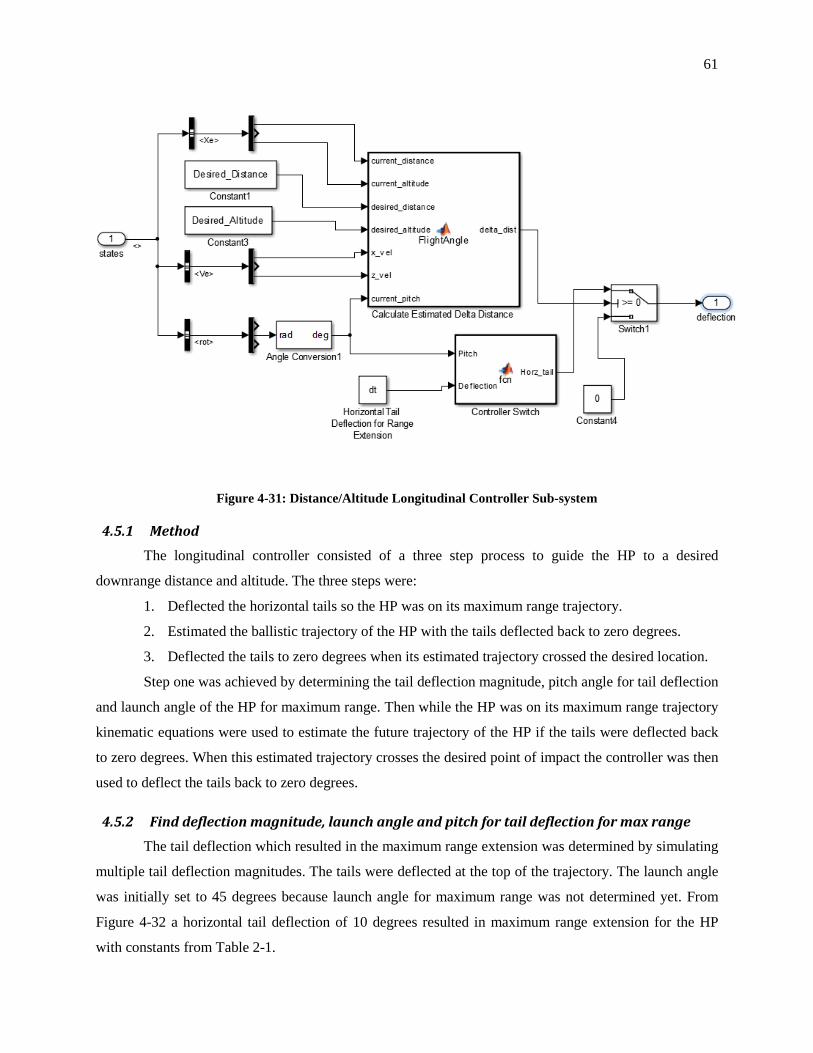
61
Figure 4-31: Distance/Altitude Longitudinal Controller Sub-system
4.5.1 Method The longitudinal controller consisted of a three step process to guide the HP to a desired
downrange distance and altitude. The three steps were:
1. Deflected the horizontal tails so the HP was on its maximum range trajectory.
2. Estimated the ballistic trajectory of the HP with the tails deflected back to zero degrees.
3. Deflected the tails to zero degrees when its estimated trajectory crossed the desired location.
Step one was achieved by determining the tail deflection magnitude, pitch angle for tail deflection
and launch angle of the HP for maximum range. Then while the HP was on its maximum range trajectory
kinematic equations were used to estimate the future trajectory of the HP if the tails were deflected back
to zero degrees. When this estimated trajectory crosses the desired point of impact the controller was then
used to deflect the tails back to zero degrees.
4.5.2 Find deflection magnitude, launch angle and pitch for tail deflection for max range The tail deflection which resulted in the maximum range extension was determined by simulating
multiple tail deflection magnitudes. The tails were deflected at the top of the trajectory. The launch angle
was initially set to 45 degrees because launch angle for maximum range was not determined yet. From
Figure 4-32 a horizontal tail deflection of 10 degrees resulted in maximum range extension for the HP
with constants from Table 2-1.

62
Figure 4-32: Horizontal Tail Deflection for Maximum Range
With the tail deflection for maximum range now determined, the pitch angle of the HP, when the
tails were deflected, that yielded the maximum range extension was determined. The pitch was used to
determine when the tails were deflected for maximum range so that the munition would not need to be
reprogrammed for launch, as investigated in (Gioia 2013). The pitch angle was varied from 10 degrees to
negative 10 degrees and it was determined that the maximum range occurs when the tails were deflected
when the projectile was at negative 3.3 degrees pitch, from Figure 4-33 and Figure 4-34.
0% 12.5% 25% 37.5% 50% 62.5% 75% 87.5% 100% 112.5% 125%0%
25%50%75%
100%125%
Alti
tude
(% o
f Max
. Alti
tude
)
Distance Downrange (Percentage of Unguided Max. Range)
0% 12.5% 25% 37.5% 50% 62.5% 75% 87.5% 100% 112.5% 125%0
10
20
Distance Downrange (Percentage of Unguided Max. Range)
Tail
Def
lect
ion
(deg
)
0% 12.5% 25% 37.5% 50% 62.5% 75% 87.5% 100% 112.5% 125%0%
25%
50%75%
100%
Distance Downrange (Percentage of Unguided Max. Range)
Vel
ocity
(% o
f Lau
nch
Vel
ocity
)
0 degree deflection5 degree deflection10 degree deflection15 degree deflection20 degree deflection

63
Figure 4-33: Find Maximum Range with Change in Deflection Pitch
Figure 4-34: Find Maximum Range with Change in Deflection Pitch (Zoomed to Max Range)
It was now important to update the initial launch angle with the launch angle for maximum range.
In Figure 4-35, the maximum range occurred from a 39.5 degree launch angle. A launch angle of 45
degrees does not allow for the maximum distance of this projectile because of drag. The projectile must
efficiently convert kinetic energy to potential energy than back to kinetic energy. With drag, the most
efficient situation was when the projectile was launched at 39.5 degrees. A 39.5 degree launch angle
yielded a 25.8% range extension over the non-guided projectile which was greater than 24.5%, the range
extension from a 45 degree launch angle.
0% 12.5% 25% 37.5% 50% 62.5% 75% 87.5% 100%112.5%125%0%
25%
50%
75%
100%
125%
Alti
tude
(% o
f Ung
uide
d M
ax. A
ltitu
de)
Distance Downrange (Percentage of Unguided Max. Range)
-10 degrees-3.3 degrees0 degrees3.3 degrees10 degrees
120% 121% 122% 123% 124% 125%0%
2%
4%
6%
8%
Alti
tude
(% o
f Ung
uide
d M
ax. A
ltitu
de)
Distance Downrange (Percentage of Unguided Max. Range)
-10 degrees-3.3 degrees0 degrees3.3 degrees10 degrees

64
Figure 4-35: Distance and Altitude of 1 to 87 degree launch angle
4.5.3 Range Extension and Guidance
The ‘Calculate Estimated Delta Distance’ sub-system from Figure 4-31 was created to determine
the difference between the required distance and the estimated distance calculated for the accelerations
caused by the tails being deflected back to zero degrees. The estimated distance was determined by
completing a force balance acting on the projectile, with the free-body diagram in Figure 4-36 then
solving the equations of motion. The sub-system contained a while loop that determined when the
projectile crossed the desired altitude along its current ballistic trajectory. At that altitude the distance
downrange was recorded. If the estimated distance from the while loop became greater than the desired
distance the switch function in Figure 4-31was used to deflect the tails back to zero degrees.
The acceleration of the projectile due to lift and drag was determined for the x and z directions.
The forces acting on the HP that effected the acceleration were lift, drag and gravitational force. The
forces were used to determine the acceleration by dividing by the projectiles mass. In equations (4-3) and
(4-4) the lift coefficient, drag coefficient and angle of attack produced was required. This data was
collected through simulation results in Section 4.5.4. The free body diagram used to determine the
accelerations was Figure 4-36 with the accelerations as equations (4-3) and (4-4). At each time step the
pitch and angle of attack were summed together, as shown in Figure 4-36. The velocity and position in the
0% 50% 100% 150%0%
25%
50%
75%
100%
125%
150%
Time(% of Unguided Flight Time for 39.5 deg Launch)
Dow
nran
ge D
ista
nce
(% o
f Max
. Ung
uide
d R
ange
for 3
9.5
deg
Laun
ch)
0% 50% 100% 150%0%
50%
100%
150%
200%
250%
Time(% of Unguided Flight Time for 39.5 deg Launch)
Alti
tude
(% o
f Max
. Ung
uide
d A
ltitu
de fo
r 39.
5 de
g La
unch
)

65
x and z direction were determined by taking the first and second derivative of the acceleration in each
direction, respectively. The velocity and position were using solved using a discrete time step (∆𝑡). The
velocities were determined by adding the velocity at the previous time step to the acceleration multiplied
by the time step in equations (4-5) and (4-6). The pitch had to be recalculated at each time step by using
equation (4-7), due to the change in velocity vector and angle of attack. Similar to calculating the
velocity, the position of the HP was calculated using equations (4-8) and (4-9).
Z
X
Drag
Lift
Velocity
Weight
Pitch
Pitch
Pitch + α
Figure 4-36: FBD used to determine accelerations on projectile
𝑎𝑧 = −𝑔 + cos(|𝑃𝑖𝑡𝑐ℎ|)𝐶𝐿
. 5𝜌𝑆𝑉2
𝑀𝑝+ sin(|𝑃𝑖𝑡𝑐ℎ|)𝐶𝐷
. 5𝜌𝑆𝑉2
𝑀𝑝 (4-3)
𝑎𝑥 = sin(|𝑃𝑖𝑡𝑐ℎ|)𝐶𝐿
. 5𝜌𝑆𝑉2
𝑀𝑝− cos(|𝑃𝑖𝑡𝑐ℎ|)𝐶𝐷
. 5𝜌𝑆𝑉2
𝑀𝑝 (4-4)
𝑉𝑧𝑖 = 𝑉𝑧𝑖−1 + 𝑎𝑧∆𝑡 (4-5)
𝑉𝑥𝑖 = 𝑉𝑥𝑖−1 + 𝑎𝑥∆𝑡 (4-6)
𝑃𝑖𝑡𝑐ℎ = tan−1 �
𝑉𝑧𝑖𝑉𝑥𝑖�+ 𝛼 (4-7)
𝑧𝑖 = 𝑧𝑖−1 + 𝑉𝑧𝑖∆𝑡 (4-8)
𝑥𝑖 = 𝑥𝑖−1 + 𝑉𝑥𝑖∆𝑡 (4-9)
4.5.4 CL, CD and AoA when tails are deflected to zero degrees
The lift coefficient, drag coefficient and angle of attack could be determined due to the tails being
deflected from ten to zero degrees using the simulator.ly to zero degrees. These values were estimated by
saving each to be used at each time step after the tails start moving to zero deflection. The vector values
were saved at a 200 Hz time step starting from the time where tails had a command to go to zero degrees

66
from 10 degrees. Figure 4-37 shows the total lift coefficient, total drag coefficient and angle of attack
after the tails were deflected to zero degrees at eight seconds.
Figure 4-37: Create Vectors of CL CD and AoA from Tail Deflection
All the variables in equations (4-3) and (4-4) were now known and were used to estimate the
ballistic trajectory of the HP. When the ballistic trajectory estimated passed through the desired point of
impact (delta_dist= 0) the tails were deflected back to zero degrees using the switch function.
4.5.5 Longitudinal Controller Testing
The inputs of two different on line-of-fire impact points were chosen to test the longitudinal
controller. The simulated results and the desired results were compared. In Figure 4-38, the unguided
trajectory was compared with the guided trajectory and the horizontal tail deflection for the targeting was
shown as well. In Figure 4-38 the desired distance was 122.5% of the unguided projectiles maximum
range at 0% maximum unguided altitude. In Figure 4-39 the desired distance was 100% of the unguided
projectiles maximum range at 50% maximum unguided altitude. The results of the simulations were
shown in Table 4-8. These figures show that the longitudinal controller was able to achieve the task of
guiding the projectile to a desired distance and altitude within 22.5 projectile diameters of the desired
location.
0 5 10-2
0
2
4
6
8
10
12
Time (sec)
Hor
izon
tal T
ail D
efle
ctio
n (d
egre
es)
0 5 10-1
-0.5
0
0.5
1
1.5
2
Time (sec)
Lift
Coe
ffici
ent
0 5 100.2
0.4
0.6
0.8
1
Time (sec)
Dra
g C
oeffi
cien
t
0 5 10-10
0
10
20
30
Time (sec)
Ang
le o
f Atta
ck (d
egre
es)

67
Figure 4-38: Longitudinal Target Distance=122.5% Max Unguided Altitude=0% Max Unguided
Figure 4-39: Longitudinal Target Distance=100% Max Unguided Altitude=50% Max Unguided
0% 25% 50% 75% 100% 125%0%
25%
50%
75%
100%
125%
Alti
tude
(% o
f Max
. Ung
uide
d A
lt.)
Downrange Distance (Percentage of Maximum Unguided Range)
0% 25% 50% 75% 100% 125%
0
5
10
Downrange Distance (Percentage of Maximum Unguided Range)
Hor
izon
tal T
ail D
efle
ctio
n(D
egre
es)
UnguidedVertical Control
0% 25% 50% 75% 100% 125%0%
25%
50%
75%
100%
125%
Downrange Distance (Percentage of Maximum Unguided Range)
Alti
tude
(% o
f Max
. Ung
uide
d A
lt.)
0% 25% 50% 75% 100% 125%
0
5
10
Downrange Distance (Percentage of Maximum Unguided Range)
Hor
izon
tal T
ail D
efle
ctio
n(D
egre
es)
UnguidedVertical Control

68
Table 4-8: Results from Longitudinal Control Simulations
Desired Distance Desired Altitude Actual Distance at Desire Altitude Distance Offset
122.5% of Unguided Max Range
0% of Max Unguided Altitude
122.39% of Unguided Max Range
11.3 projectile diameters
100% of Unguided Max Range
50% of Max Unguided Altitude
99.8% of Unguided Max Range
22.5 projectile diameters
4.6 Guidance Simulation Results Now that all three controllers have been designed and tested individually, the guidance capability
of the 40 mm HP was simulated. In the first test, all three controllers’ interaction with each other was
investigated. Their interaction was investigated by simulating the projectile with an initial roll rate of 62.5
Hz and having the controller de-spin, roll-level and guide the HP to a desired point of impact. The desired
impact point simulated was 100% of the maximum unguided range downrange, at 28.3% of the maximum
unguided altitude and 1500 projectile diameters right offset from the Line of Fire. Figure 4-40 shows the
distance, altitude and line-of-fire offset of the flight path as well as the roll angle and the deflections made
by the each set of tails. Results of this simulation show the projectile was off of the desire impact location
by 14.3 projectile diameters.
Figure 4-40: Simulation of Three Controllers Combined
0% 25% 50% 75% 100%0%
25%
50%
75%
100%
125%
Downrange Distance (Percentage of Maximum Unguided Range)
Alti
tude
(% o
f Max
. Ung
uide
d A
lt.)
0% 25% 50% 75% 100%0
500
1000
1500
2000
Downrange Distance (Percentage of Maximum Unguided Range)
Dis
tanc
e of
f Lin
e of
Fire
(# o
f Pro
ject
ile D
iam
eter
s)
0% 25% 50% 75% 100%0
5
10
Downrange Distance (Percentage of Maximum Unguided Range)Hor
izon
tal T
ail D
efle
ctio
n (d
eg)
0% 25% 50% 75% 100%-10
-5
0
5
Downrange Distance (Percentage of Maximum Unguided Range)
Ver
tical
Tai
l Def
lect
ion
(deg
)
0% 25% 50% 75% 100%-200
-100
0
100
200
Downrange Distance (Percentage of Maximum Unguided Range)
Rol
l Ang
le (d
eg)
0% 25% 50% 75% 100%-10
-5
0
5
10
Downrange Distance (Percentage of Maximum Unguided Range)
Rol
l Tai
l Def
lect
ion
(deg
)
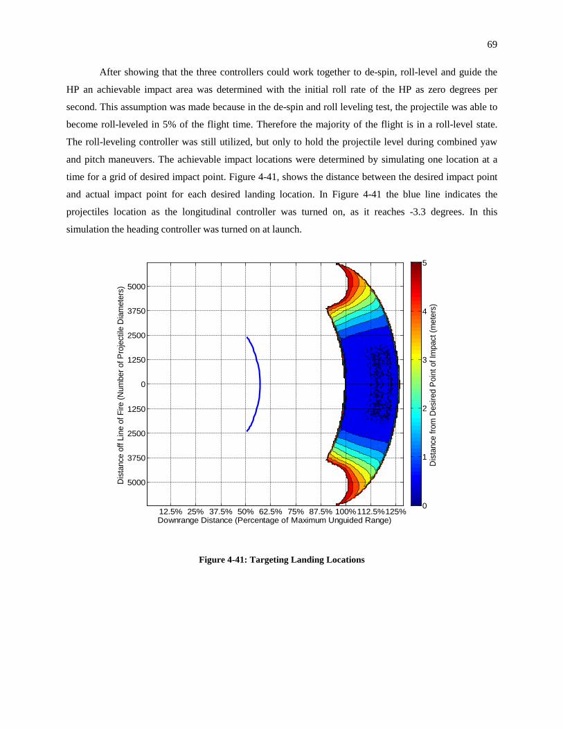
69
After showing that the three controllers could work together to de-spin, roll-level and guide the
HP an achievable impact area was determined with the initial roll rate of the HP as zero degrees per
second. This assumption was made because in the de-spin and roll leveling test, the projectile was able to
become roll-leveled in 5% of the flight time. Therefore the majority of the flight is in a roll-level state.
The roll-leveling controller was still utilized, but only to hold the projectile level during combined yaw
and pitch maneuvers. The achievable impact locations were determined by simulating one location at a
time for a grid of desired impact point. Figure 4-41, shows the distance between the desired impact point
and actual impact point for each desired landing location. In Figure 4-41 the blue line indicates the
projectiles location as the longitudinal controller was turned on, as it reaches -3.3 degrees. In this
simulation the heading controller was turned on at launch.
Figure 4-41: Targeting Landing Locations
Dis
tanc
e of
f Lin
e of
Fire
(Num
ber o
f Pro
ject
ile D
iam
eter
s)
Downrange Distance (Percentage of Maximum Unguided Range)
5000
3750
2500
1250
0
1250
2500
3750
5000
12.5% 25% 37.5% 50% 62.5% 75% 87.5% 100%112.5%125%
Dis
tanc
e fro
m D
esire
d Po
int o
f Im
pact
(met
ers)
0
1
2
3
4
5

70
From the simulation it was seen that the range was extended 25.8% along the line of fire and was
also able to turn up to 6250 projectile diameters off the line of fire. In Figure 4-41 it was seen the
accuracy decreased towards the outer target areas. A greater error could occur in the outer ranges of
desired impact points since the drag and lift data estimation calculated in Section 4.5.4 were different than
the actual values. These differences could occur from vertical tail contributions that were not applied
when estimation the drag and lift coefficients.
When considering a projectile like a 40 mm HP it was important to know that the impact velocity
has not been greatly changed from that of the original non-guided munition. The kinetic energy of the
projectile upon impact causes a particular fragmentation pattern. By decreasing the kinetic energy in
which the projectile strikes the ground, the fragmentation pattern changes from the designed pattern.
Figure 4-42 shows the impact velocity for the projectile during the same simulation test as Figure 4-41,
where the colorbar depicts the velocity as a percentage of the impact velocity for the unguided simulation.
Figure 4-42: Final Velocity of the Projectile
Dis
tanc
e of
f Lin
e of
Fire
(Num
ber o
f Pro
ject
ile D
iam
eter
s)
Downrange Distance (Percentage of Maximum Unguided Range)
5000
3750
2500
1250
0
1250
2500
3750
5000
12.5% 25% 37.5% 50% 62.5% 75% 87.5% 100%112.5%125%
Impa
ct V
eloc
ity (P
erce
ntag
e of
Ung
uide
d V
eloc
ity)
70%
75%
80%
85%
90%
95%
100%

71
The amount of tail control required for each desired impact location was also an important
characteristic of the guided flight to be shown. By knowing the areas in which maximum deflection
magnitude was necessary the desired impact point area could be narrowed for a gust situation. If the
projectile takes maximum tail deflection to get to a specific impact point in a gust free environment, it is
not realistic during an actual launch since any gust it needed to control against would cause the projectile
to not be able to achieve its point of impact. In Figure 4-43, the tail deflection average magnitude shows
the areas where the most tail deflection was required to hit its desired point of impact. The deflection
magnitude was calculated as the average magnitudes of the vertical and horizontal tail deflections. The
colorbar of Figure 4-43 shows the magnitude of tail deflection, in degrees, required for each desired point
of impact.
Figure 4-43: Magnitude of Average Tail Deflections
The M781 projectile was modified with a cruciform tail section as described in Section 3.4 then
modeled using an aerodynamic build-up. Each of the four tails had an adjustable angle of attack and was
modeled with a servo delay. With the use of a de-spin and roll-leveling controller the tails were deflected
to steadily de-spin and roll-level the HP in 5% of its flight time. Once the HP was roll-leveled, guidance
maneuvering was begun. A heading controller was created to maneuver the HP to a particular heading
Dis
tanc
e of
f Lin
e of
Fire
(Num
ber o
f Pro
ject
ile D
iam
eter
s)
Downrange Distance (Percentage of Maximum Unguided Range)
5000
3750
2500
1250
0
1250
2500
3750
5000
12.5% 25% 37.5% 50% 62.5% 75% 87.5% 100%112.5%125%
Ave
rage
Mag
nitu
de o
f Tai
l Def
lect
ion
(Deg
rees
)
0
2.5
5
7.5
10
12.5

72
angle or distance from the line of fire using its two vertical tails. Longitudinal control was achieved with a
controller which deflected the HP’s horizontal tails to 10 degrees then back to zero as the HP’s ballistic
trajectory crossed its desired downrange distance and altitude. The three controllers combined were
simulated and results showed that the HP could be de-spun, roll-leveled and guided to 0.57 meters of its
desired point of impact. When the HP was not spinning at launch the effect of the longitudinal and
heading controllers were simulated to determine an area of achievable impact points. Simulation results
show that the HP could be guided to impact points up to 25% beyond the range of the baseline M781 and
6250 projectile diameters off the line of fire.
4.7 Disturbance Rejection of Controllers An understanding of disturbances encountered, such as a side gust during guidance, is critical to
ensure that the desired flight was still achieved. Disturbance rejection for guidance control was analyzed
by adding a cross wind vector to the freestream velocity vector in the simulation.
Two cases of wind were investigated with multiple wind velocities to determine change in
distance offset to the desired point of impact from the wind free case. The first case consists of a two
second wind gust occurring between two and four seconds of flight time. The wind gust velocities over a
two second gust were chosen to be two, five and ten meters per second. The gust duration was chosen
from an average gust time found in (Beljaars 1987). The three velocity values were chosen to show how
increasing velocity effected guidance. Also a constant sustained velocity wind case was investigated for
two, five and ten meters per second sustained wind throughout the entire flight. The wind was simulated
to be blowing normal to the line of fire from left to right. The wind velocity in this case was applied
normal to the line of fire and needed to be transformed from earth fixed to body coordinate system using
the horizontal wind model block in the aerospace toolbox of Simulink.

73
Three points of impact were chosen as the desired locations for the wind gust and sustained wind
cases. The desired impact points were compiled in Table 4-9. Location 1, 105% max unguided range and
5000 projectile diameters left, was chosen because it is an achievable impact location which was on the
far left end of the impact grid and to reach this location the projectile would be going into the direction of
the wind. Location 2, 105% max unguided range and 5000 projectile diameters right, was chosen because
it was an achievable impact location on the far right of the impact grid and in the same direction as the
wind. Determining if the HP could hold on the line of fire and reach a point with no offset was shown by
choosing Location 3, 125% max unguided range. The ground tracks for each case were shown in Figure
4-44 through Figure 4-49 to show how the projectile deviated from its trajectory with and without wind
while being guided to the desired impact location. The percentage difference for each case with wind was
calculated using equation (4-10), where offset with wind (OffWind) was compared with the windless
impact offset (OffNoWind).
Table 4-9: Desired Impact Locations for Disturbance Rejection
Location Number
Desired Down Range Distance
Desired Location off Line of Fire
1 105% Max Unguided Range 5000 Projectile Diameters Left
2 105% Max Unguided Range 5000 Projectile Diameters Right
3 125% Max Unguided Range On-line
�𝑂𝑓𝑓𝑊𝑖𝑛𝑑 − 𝑂𝑓𝑓𝑁𝑜𝑊𝑖𝑛𝑑
𝑂𝑓𝑓𝑁𝑜𝑊𝑖𝑛𝑑� × 100% (4-10)

74
4.7.1 Two Second Wind Gust The case in which a two second wind gust was added to the model was simulated first to predict
the performance due to different gust velocities. The first simulation in this case was used to predict the
performance of the HP when the desired impact location required the HP to fly into the wind gust. The
first location desired was for the HP to land at 105% maximum unguided range downrange and 5000
projectile diameters left off the line of fire. When the HP was simulated without wind gust it was able to
land 104 projectile diameters off of the desired point of impact. As the wind velocity was increased the
projectile was simulated to land up to 18% farther from the desired location, Figure 4-44.
Table 4-10: Impact offset due to Wind Gust to Desired Location 1
Wind Speed
(m/s)
Distance Off Desired
Impact
(projectile diameters)
% Difference
from 0 m/s
0 104
2 107.5 3%
5 112.5 8%
10 122.5 18%
Figure 4-44: Ground Track of HP with Wind Gust to Desired Location 1

75
The second simulation in this case was used to predict the performance of the HP when the
desired impact location required the HP to fly with the wind gust. The second location desired was for the
HP to land at 105% maximum unguided range downrange and 5000 projectile diameters right off the line
of fire. When the HP was simulated without wind gust it was able to land 104 projectile diameters off of
the desired point of impact. As the wind velocity was increased the projectile was simulated to land up to
10% closer to the desired location, Figure 4-45.
Table 4-11: Impact offset due to Wind Gust to Desired Location 2
Wind Speed
(m/s)
Distance Off Desired
Impact
(projectile diameters)
% Difference
from 0 m/s
0 104
2 101 -3%
5 96.5 -7%
10 93.5 -10%
Figure 4-45: Ground Track of HP with Wind Gust to Desired Location 2

76
The final simulation in this case was used to predict the performance of the HP when the desired
impact location required the HP remain on the line of fire. The third location desired was for the HP to
land at 125% maximum unguided range downrange on the line of fire. When the HP was simulated
without wind gust it was able to land 14.3 projectile diameters off of the desired point of impact. As the
wind velocity was increased the projectile was simulated to land up to 44% farther from the desired
location, Figure 4-46.
Table 4-12: Impact offset due to Wind Gust to Desired Location 3
Wind Speed
(m/s)
Distance Off Desired
Impact
(projectile diameters)
% Difference
from 0 m/s
0 14.3
2 16.3 14%
5 19.3 35%
10 20.5 44%
Figure 4-46: Ground Track of HP with Wind Gust to Desired Location 3

77
4.7.2 Sustained Cross Wind The second case of sustained wind was added to the model and used to predict the performance of
the HP due to different sustained wind velocities. The first simulation in this case was used to predict the
performance of the HP when the desired impact location required the HP to fly into the sustained wind.
The first location desired was for the HP to land at 105% maximum unguided range downrange and 5000
projectile diameters left off the line of fire. When the HP was simulated without wind it was able to land
104 projectile diameters off of the desired point of impact. As the wind velocity was increased it was seen
that with wind of two meters per second the projectile was simulated to land up to 62% closer to the
desired location. However, as the wind velocity was increased up to ten meters per second the HP was
simulated to land 961% farther from desired, Figure 4-47.
Table 4-13: Impact offset due to Sustained Wind to Desired Location 1
Wind Speed
(m/s)
Distance Off Desired Impact
(projectile diameters)
% Difference
from 0 m/s
0 104
2 39.3 -62%
5 171 64%
10 1104 961%
Figure 4-47: Ground Track of HP with Sustained Wind to Desired Location 1

78
The second simulation in this case was used to predict the performance of the HP when the
desired impact location required the HP to fly in the same direction as the sustained wind. The second
location desired was for the HP to land at 105% maximum unguided range downrange and 5000 projectile
diameters right off the line of fire. When the HP was simulated without wind it was able to land 104
projectile diameters off of the desired point of impact. As the wind velocity was increased the projectile
was simulated to land up to 552% farther from the desired location, Figure 4-48.
Table 4-14: Impact offset due to Sustained Wind to Desired Location 2
Wind Speed
(m/s)
Distance Off Desired
Impact
(projectile diameters)
% Difference
from 0 m/s
0 104
2 193.3 86%
5 353 239%
10 678.3 552%
Figure 4-48: Ground Track of HP with Sustained Wind to Desired Location 2
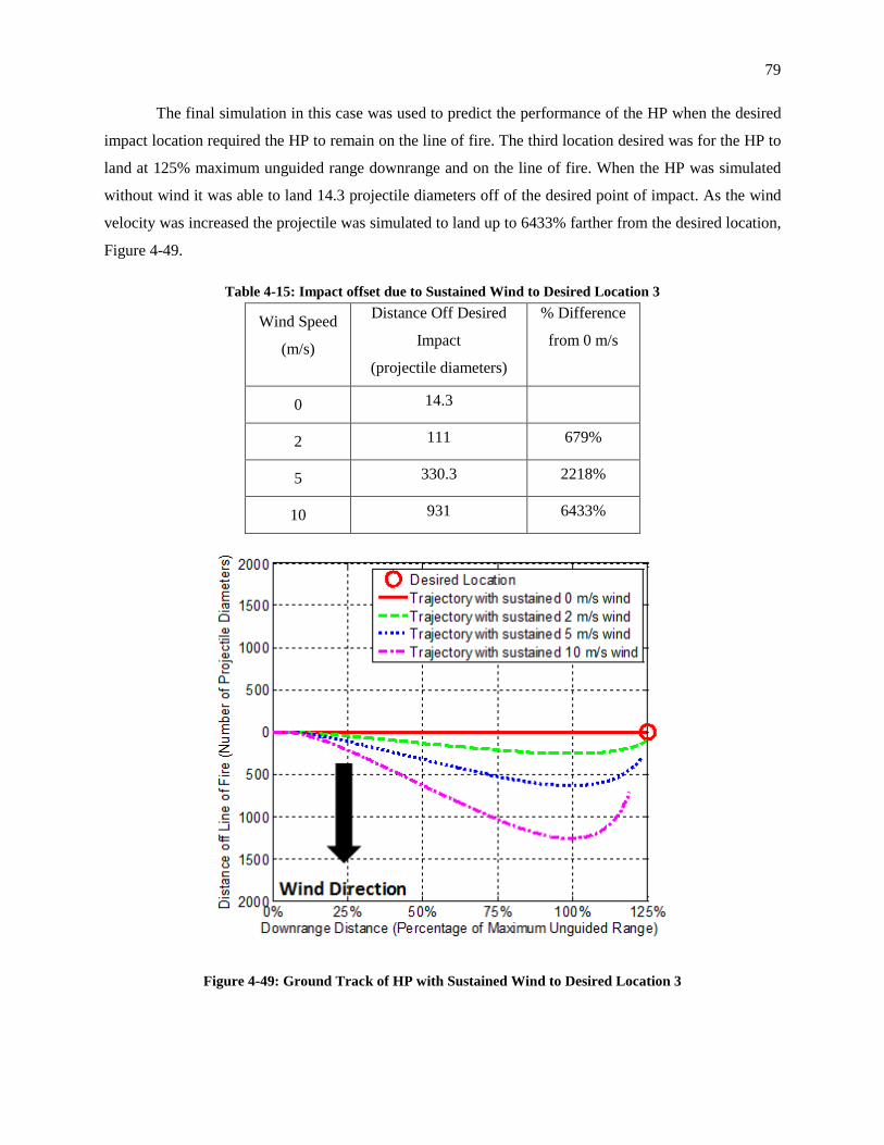
79
The final simulation in this case was used to predict the performance of the HP when the desired
impact location required the HP to remain on the line of fire. The third location desired was for the HP to
land at 125% maximum unguided range downrange and on the line of fire. When the HP was simulated
without wind it was able to land 14.3 projectile diameters off of the desired point of impact. As the wind
velocity was increased the projectile was simulated to land up to 6433% farther from the desired location,
Figure 4-49.
Table 4-15: Impact offset due to Sustained Wind to Desired Location 3
Wind Speed
(m/s)
Distance Off Desired
Impact
(projectile diameters)
% Difference
from 0 m/s
0 14.3
2 111 679%
5 330.3 2218%
10 931 6433%
Figure 4-49: Ground Track of HP with Sustained Wind to Desired Location 3

80
Results from the wind disturbance simulations showed that the accuracy was reduced when wind
occurred for each desired location and both wind cases except the gust case for the desired location 2.
This case resulted in the HP being closer to the desired point of impact because the gust helped to push
the HP towards the desired impact point. Even though accuracy was decreased to guidance controller was
still able to maneuver the HP towards the desired location. Viewing the ground tracks of Figure 4-47 and
Figure 4-49, it was seen that the HP did not miss the desired point of impact by being off line but it ended
up being short in most cases. This was because the HP did not have a propulsion system and when flying
into the wind the projectile had a greater amount of drag, reducing range.

81
Chapter 5 Conclusions and Future Work
5.1 Summary In this thesis, a method was sought to use deflectable control surfaces in combination with a
guidance system to maneuver a HP to a desired impact point, while maintaining stability and using the
body as a lifting surface. This method was then used to adequately size tail surfaces on a M781 40 mm
round to test stability could be ensured. The M781 is a spin-stabilized projectile that needs to be roll-level
before guidance could be employed so that the body could be pitched up and used as a lifting surface.
Pitch, roll and yaw controllers were thus required to deflect the local angle of attack of the tail surfaces to
de-spin and roll-level the HP before maneuvering it to a desired impact point.
The process of creating a control method was begun by collecting aerodynamic data and
specifications from a 40 mm M781. A model was then created with the use of Simulink’s aerospace
toolbox to solve the equations of motion. Forces and moments were estimated due to aerodynamic
coefficients. Then a build-up of aerodynamic coefficients was generated for the M781 equipped with tail
surfaces. The tail surface size was determined to meet the de-spin requirement of being roll-leveled in less
than 2 seconds and to ensure the HP was statically and dynamically stable. Tail control surfaces were
chosen for this HP because of their tendency to stabilize a statically unstable projectile, by shifting the
center of pressure aft of the center of gravity. A cruciform tail section with each tail having a chord of 20
mm and a span of 30 mm was required to have the projectile de-spin and roll-level in 1.64 seconds. The
tail surface area also ensured that the HP was statically and dynamically stable.
A roll controller was developed next to deflect the tail surfaces to de-spin and roll-level the HP.
The roll controller was developed with two PID controllers; one was used to steadily reduce the roll rate
and the second to roll-level the projectile. Each PID controller was tuned through an iterative process. An
adaptive transition point between the two controllers was determined to reduce time required for the
projectile to become roll-leveled.
An important step in this method was to determine technique to be used for guidance. Guidance
was divided into two parts: longitudinal and heading control. Heading control was achieved through a
PID feedback control system. Feedback control for heading maneuvers was used to deflect the vertical
tails so the HP reached a desired distance off the line of fire or a specified heading azimuth. The PID gain
values were determined for this controller by using the built in tuning function in Simulink. With the use
of the heading controller, the HP was able to be maneuvered up to 6250 projectile diameters, about 33
degrees, off the line of fire and land within 125 projectile diameters of the desired impact point. A
longitudinal controller was developed to deflect the horizontal tails to a maximum deflection of 10
degrees, nosing the body up. The HP was nosed up so that the body could be used as a lifting surface

82
extending range. Next, the controller was used to deflect the horizontal tails back to zero degrees when
the estimated trajectory of the projectile crossed the desired impact point. The longitudinal component of
guidance was able to achieve an increase in range of 25.8% as compared to a standard unguided M781.
By following the method described, a control system was determined for a specified tail surface geometry
applied to a 40 mm M781 for stability and guidance.
The contribution of this work to the field of engineering was the use of a dual mode controller to
de-spin and roll-level a HP and the use of decoupled heading and longitudinal control. Decoupled control
was important so that the body could be used as a lifting surface for range extension and the tails could be
used to maneuver the HP to a desired point of impact.
5.2 Future Work In extension to the research conducted for the Hybrid Projectile project on the 40 mm munition a
few additional tasks are recommended. First, the projectile designed in this study needs to be fabricated
and flight tested to determine if the controllers designed in simulation will work in a real flight scenario.
Further aerodynamic data should be investigated, through steady-state CFD and static experimental tests,
for the combined geometry of both body and tails. Transient experimental tests could be used to verify the
simulation results by using a wind tunnel and a spinning rig to test the de-spin controller. The wind tunnel
could also be useful with load cell data to determine if forces and moments created by the tail surfaces are
adequate for guidance.
Further development can also be done on the verification model of Section 3.3 in which this HP
could have deflectable tails applied similar to the HP in Figure 5-1. This HP can be equipped with the Px4
autopilot and used to deflect the control surfaces. Adding control capability to the autopilot requires that
the control algorithms from Matlab be discretized. Sensors from the autopilot can be used determine the
states of the projectile and the autopilot also has output capabilities. Simulink can then be used to create a
source code which can be loaded onto autopilot and used to deflect the control surfaces, guiding the HP.

83
Figure 5-1: Example concept of Tail modification for a HP
Next, the stowable wing designs which have been investigated for the 40 mm HP could be
applied for further range extension. With the tail surfaces designed the range was only increased by
25.8%, but could be extended more with larger lifting surfaces. From a simple lift to drag ratio
comparison the lift to drag ratio of the HP with the tails deflected was approximately 1.7:1 resulting in a
glide slope of 30 degrees. However, with wings added the total lift to drag ratio could be closer to 4:1
with a glide slope of 14 degrees. If the wings are deployed at the same pitch angle as the tails were
deflected the range could be extended at least 50% beyond the standard unguided 40 mm M781
(Hamburg 2010). Wings also can add instability to the HP which can be corrected through the use of the
method described in this thesis. Having a HP with wings and control surfaces allows for the projectile to
be guided and achieve further range extension.

84
References ALS Technologies. "M781 Product Data Sheet". Bull Shoals, AR, Jun. 2009.
<http://static.alstechnologies.com/specs/MEI/M781.pdf>. Barrowman, James. Calculating the Center of Pressure of a Model Rocket. Technical Information Report
- 33. Phoenix, Arizona: Centuri Engineering Company, n.d. Beljaars, A. C. M. . "The Influence of Sampling and Filtering on Measured Wind Gusts." Journal of
Atmospheric and Oceanic Technology (1987): 613-626. Web. Carlucci, Donald E. and Sidney S. Jacobson. Ballistics: Theory and Design of Guns and Ammunition.
Boca Raton, FL: CRC/Taylor & Francis Group, 2008. Print. Christiansen, Reed Siefert. Design of an Autopilot for Small Unmanned Aerial Vehicles. MS Thesis,
Brigham Young University, 2004. Cooke, Gary W. "40mm Low-Velocity Grenades." 25 Feb. 2010.
<http://www.inetres.com/gp/military/infantry/grenade/40mm_ammo.html#M781>. Dupuis, Alain. "Aeroballistics Range Tests of a 40 mm Projectile." 23rd International Symposium on
Ballistics. Tarragona, Spain, (2007). 705-712. Exploration, Stellar. Stellar-Exploration. 4 June 2011. 2013. <http://www.stellar-
exploration.com/#!40mm-guided-grenade>. FAS Military Analysis Network. "M203 40mm Grenade Launcher." 22 February 2000. Federation of
American Scientists. 22 March 2014. <http://www.fas.org/man/dod-101/sys/land/m203.htm>. "Flight Equations with Drag." 28 July 2011. National Aeronaitics and Space Administration. 29 June
2013. <http://www.grc.nasa.gov/WWW/k-12/airplane/flteqs.html>. Fresconi, F, et al. "Flight mechanics of a novel guided spin-stabilized concept." Proc. IMechE Vol. 226
Part G: J. Aerospace Engineering (2011): 327-340. Fresoni, F and P Plostins. "Control mechanism strategies for spin-stabilized projectiles." Proc. IMechE
Vol. 224 Part G: J. Aerospace Engineering (2011): 979-991. Gioia, Christopher J. Hybrid Projectile Body Angle Estimation for Selectable Range Increase. MS Thesis,
West Virginia University, 2013. Gkritzapis, Dimitrios N.; Margaris, Dionissios P.; Panagiotopoulos, Elias E.; Kaimakamis, George, et al.
"Prediction of the Impact Point for Spin and Fin Stabilized Projectiles." WSEAS Transactions on Information Science and Applications Volume 5. Issue 12 (2008): 1667-1676.
Gregorek, Gerald M. Aerodynamic Drag of Model Rockets. Penrose, Colorado: Estes Industries, Inc., 1970.
Haiyang Chao, Yongcan Cao, YangQuan Chen. "Autopilots for Small Fixed-Wing Unmanned Air Vehicles: A Survey." IEEE International Conference on Mechatronics and Automation. Harbin, China, 2007. 3144-3149.
Hamburg, Shanti. Conceptual and Preliminary Design of a Stowable Ruggedized Micro Air Vehicle. MS Thesis, West Virginia University, 2010.
Hasnink, Kelly. "Mortar Guidance Kit (MGK)." 2010 Joint Armaments Conference. 2010. <http://www.dtic.mil/ndia/2010armament/TuesdayCumberlandKellyHanink.pdf>.
Ives, John M. "Armored Cavalry Mortars: Operations and Myths." ARMOR November-December 2001. 22-26.
Jie, Cheng; Xiaoming, Wang; Jiyan, Yu; Wenjin, Yao. "On the Response of Spin Stabilized Projectile to Side Force by Angular Motion and Impact." 27th International Symposium on Ballistics. Freiburg, Germany: DEStech Publications, Inc., 2013. 225-232.

85
Langdon, S.D and W.V. Cross. Fixed Wing Stability and Control: Theory and Flight Test Techniques. Defense Technical Information Center, 1977.
Larsen, Erik, et al. Ranger Knowledge: The All-Inclusive Study Guide for Rangers. Manhattan: St. Martins Press, 2013.
Lovas, Andre, et al. DARPA SCORPION Program Transition to Army Lethality ATO Program: A Success Story. Picatinny: ARL, 2009.
Lyon, David H. "Development of a 40mm Nonlethal Cartridge." DT/FL Research Journal (1997). Manole, L; Logsdon, E; Palathingal, M; Sebasto, A. Gun launched hybrid projectile. United States of
America: Patent 8115149. 21 Jul 2009. Martinez, Marcelo, Nicolas Bruno and Dr. Roy Kelly. "27th International Symposium on Ballisitcs." 27th
International Symposium on Ballisitcs. Freiburg, Germany: DEStech Publications. Inc, 2013. 302-313.
Matlab. "MATLAB R2013a (8.1.0.604)." Products and Services Online. The MathWorks Inc., 2014. <http://www.mathworks.com/products/?s_tid=gn_ps>.
McMichael, J; Lovas, A; Plostins, P; Sahu, J; Brown, G; Glezer, A. "Microadaptive Flow Control Applied to a Spinning Projectile." 2nd AIAA Flow Control Conference. Portland, Oregon: AIAA, 2004. 30.
Milinovic, Momcilo; Jerkovic, Damir; Jeremic, Olivera; Kovac, Mitar. "Experimental and Simulation Testing of Flight Spin Stability for Small Caliber Cannon Projectile." Strojniški vestnik - Journal of Mechanical Engineering (2012): 394-402.
MLM International. 40 mm Low Velocity M781 Practice Grenade. Washington Grove, MD, 2005. <http://www.mlmintl.com/40mmM781.pdf>.
Niskanen, Sampo. Development of an Open Source model rocket simulation. MS Thesis, Helsinki University of Technology, 2009.
Phillips, Warren F. Mechanics of Flight 2nd Edition. Hoboken, NJ: John Wiley & Sons, Inc., 2010. PX4 Autopilot. n.d. 24 September 2013. <https://pixhawk.ethz.ch/px4/modules/px4fmu>. Ramezani, Roozbeh Falah. Non-linear Modeling and Control of Unmanned Aerial Vehicle. MS Thesis,
American University of Sharjah, 2012. Raymer, Daniel P. Aircraft Design: A Conceptual Approach. Reston, Virginia: American Institute of
Aeronautics and Astronautics, Inc., 1999. Print. Roskam, Jan. Aircraft Flight Dynamics and Automatic Flight Controls. Lawrence, KS: DARcorporation,
2003. Print Roskam, Jan. Methods for Estimating Stability and Control Derivatives of Conventional Subsonic Planes.
Lawrence, Kansas: University of Kansas, 1971. Print. "Torayca." 26 November 2002. T300 Data Sheet. 27 March 2014.
<http://www.toraycfa.com/pdfs/t300datasheet.pdf>. Vogel, William L. Numerical Flight Testing of a Tube-launched Transformable Micro Air Vehicle. MS
Thesis, West Virginia University, 2012. White, Frank M. Viscous Fluid Flow Third Edition. New York, NY: The McGraw-Hill Companies, Inc.,
2006. Print. Wilhelm, Jay P.; Jackson, Edward R; Browning, Patrick; Huebsch, Wade; Mucino, Victor; Gautam,
Mridul. "Flight Simulation of a hybrid projectile to estimate the impact of launch angle on range extension." ASME 2012 International Mechanical Engineering Congress & Exposition. Houston, 2012. 615-620.
Wilson, Michael J. Projectile Navigation and the Application on Magnetometers. Ann Arbor: ProQuest Information and Learning Company, 2007. Print.

86
Appendix AAnalyzing Stability of the M781 M781 Gyroscopic Stability
𝑆𝑔 =𝐼𝑥𝑥2 𝑝2
2𝜌𝐼𝑦𝑦𝐴𝑟𝑒𝑓𝑑𝑉2𝐶𝑚𝛼
Where p is the roll rate in radians per second
𝑺𝒈 =(5.4412×10⁻⁵)2(392.7)2
2(1.2)(1.19215×10⁻⁴)(0.126)(0.04)(762)(1.564)= 𝟑.𝟓𝟏
Gyroscopically Stable
M781 Dynamic Stability
𝑆𝑑 =2�
𝜌𝐴𝑟𝑒𝑓𝑑32𝐼𝑦𝑦
��𝐶𝐿𝛼 + � 𝐼𝑥𝑥𝑚𝑎𝑠𝑠𝑑2
−2
𝐶𝑚𝑝𝛼�
�𝜌𝐴𝑟𝑒𝑓𝑑
2𝑚 ��𝐶𝐿𝛼 − 𝐶𝐷 − � 𝐼𝑦𝑦𝑚𝑎𝑠𝑠𝑑2
−2
𝐶𝑚𝑞�
𝑆𝑑 =
2 �(1.2)(0.126)(. 043)2(1.19215×10⁻⁴) ��2.166 + �5.4412×10⁻⁵
. 205(. 042)
−2
(−.1325)�
�(1.2)(0.126)(.04)2(.205) ��2.166− 0.2775−�1.19215×10⁻⁴
. 205(. 042)
−2
(−5.73)�= 6.29
Inequality for Dynamic Stability
1𝑆𝑔
> 𝑆𝑑(2− 𝑆𝑑)
13.51
> 6.29(2− 6.29)
𝟎.𝟐𝟖𝟓 > −𝟐𝟔.𝟗𝟖
Dynamically Stable
M781 Static Stability
𝑀 = �𝜌𝑆𝑑3
2𝐼𝑦𝑦�𝐶𝑚𝛼
𝑀 = �(1.2)(.126). 043
2(1.19215×10⁻⁴)�1.564 = 0.634
Statically Unstable

87
Appendix B Hand Calculations for Assumption of Tails Not Affecting Mass Properties
Calculate the Static Margin (SM) for the baseline 40 mm. Numbers used are cited in text.
𝑆𝑀���� = −�𝐶𝑚𝛼𝐶𝐿𝛼
� = −�0.02730.0378
� = −0.722 (Roskam 2003)�
𝑆𝑀 = 𝑆𝑀����ℓ𝑟𝑒𝑓 = −0.722 × 0.1𝑚 = −72.2𝑚𝑚
This yields a non-statically stable SM.
𝑆𝑀 = 𝑋𝐴𝐶 − 𝑋𝐶𝐺
The CG location for the 40 mm was found to be 60.41% back from the nose, meaning:
𝑋𝐶𝐺 = ℓ𝑇𝑜𝑡𝑎𝑙0.6041 = 86.4𝑚𝑚 𝑓𝑟𝑜𝑚 𝑛𝑜𝑠𝑒
𝑤ℎ𝑒𝑟𝑒 ℓ𝑇𝑜𝑡𝑎𝑙 = ℓ𝑇𝑎𝑖𝑙 +12𝑐𝑟 = 143𝑚𝑚
The AC can be calculated as:
𝑋𝐴𝐶𝐵𝑎𝑠𝑒𝑙𝑖𝑛𝑒 = 𝑆𝑀 + 𝑋𝐶𝐺 = −72.2 + 86.4 = 14.2𝑚𝑚 𝑓𝑟𝑜𝑚 𝑛𝑜𝑠𝑒
143 mm
14.2 mm
86.4 mm
AC CG
Find the Difference in CG location due to tails being added.
Assumption: Tails are made of Carbon Fiber Sheeting, 1/16th inch thick
Density of Carbon Fiber (T300) 1.76g/cm3 (Torayca 2002)
Total Volume and Mass of Tail Material
𝑉𝑜𝑙 = 4(0.159 ∗ 2.0 ∗ 3.0) = 3.81𝑐𝑚3
𝑀𝑎𝑠𝑠𝑇𝑎𝑖𝑙𝑠 = 𝜌𝐶𝐹𝑉𝑜𝑙 = 1.76 × 3.81 = 6.7𝑔𝑟𝑎𝑚𝑠
Calculate CG Location with Tails

88
143 mm
86.4 mm
Baseline Mass
87.9 mm
TailMass
133 mm
Baseline w/ Tails Mass
𝑋𝐶𝐺𝐵𝑎𝑠𝑒𝑙𝑖𝑛𝑒 𝑤/ 𝑇𝑎𝑖𝑙𝑠 =�𝑚𝐵𝑎𝑠𝑒 × 𝑋𝐶𝐺𝐵𝑎𝑠𝑒��𝑚𝑇𝑎𝑖𝑙𝑠 × 𝑋𝐶𝐺𝑇𝑎𝑖𝑙𝑠�
𝑚𝑇𝑜𝑡𝑎𝑙=
(205 × 86.4) + (6.7 × 133)(205 + 6.7) = 87.9 𝑚𝑚
Static Margin for the projectile with Tails
𝑆𝑀���� = −�𝐶𝑚𝛼
𝐶𝐿𝛼� = −�
𝐶𝑚𝛼𝐵𝑜𝑑𝑦+ 𝐶𝑚𝛼𝑇𝑎𝑖𝑙𝑠
𝐶𝐿𝛼𝐵𝑜𝑑𝑦 + 𝐶𝐿𝛼𝑇𝑎𝑖𝑙𝑠� = .3196
This yields a -statically stable SM. This was what was also seen from Figure in text.
𝑆𝑀𝑇𝑎𝑖𝑙𝑠 = .3196 ∗ .1𝑚 = 31.96𝑚𝑚
Find how much the AC moved by adding tails to the projectile.
𝑋𝐴𝐶𝐵𝑎𝑠𝑒𝑙𝑖𝑛𝑒 𝑤/ 𝑇𝑎𝑖𝑙𝑠 = 𝑆𝑀𝑇𝑎𝑖𝑙𝑠 + 𝑋𝐶𝐺𝑇𝑎𝑖𝑙𝑠 = 32 + 87.9 = 119.9𝑚𝑚
The AC shifted 105.7mm from adding tails while the CG only moved 1.5mm. The shift in CG was ignored since its shift was 1.4% of the magnitude in the AC shift.
Calculate the effect of Tail Mass on the Moment of Inertia.
𝐼𝑥𝑥𝑀781 = 5.4412 × 10⁻⁵ 𝑘𝑔 𝑚2
𝐼𝑥𝑥𝑀781 𝑤/ 𝑇𝑎𝑖𝑙𝑠 = 𝐼𝑥𝑥𝑀781 + 𝑚𝑇𝑎𝑖𝑙𝑠𝑟𝑇𝑎𝑖𝑙𝑠2
rTails is the moment arm for the center of mass about the x axis of the tails.
𝑟𝑇𝑎𝑖𝑙𝑠 =𝑑𝑖𝑎
2+𝑠𝑝𝑎𝑛𝑇𝑎𝑖𝑙𝑠
2= 0.02𝑚 + 0.015𝑚 = 0.035𝑚
𝐼𝑥𝑥𝑀781𝑤𝑇𝑎𝑖𝑙𝑠= 5.4412 × 10⁻⁵ 𝑘𝑔 𝑚2 + 0.0067𝑘𝑔 (0.035𝑚)2 = 6.262 × 10⁻⁵ (13% 𝑖𝑛𝑐𝑟𝑒𝑎𝑠𝑒)
With the mass of the tails considered the de-spin time was only effected by 2% of the flight time. So the assumption was made that mass would be ignored.

89
Appendix C CG and AC Calculation of Verification Model
Calculating CG on Test Projectile
ComponentMass
(grams)Distance From Nose
to CG of component (mm) Distance x Mass (g mm)Body 32.7 99.5 3253.65Nose 23.5 40.1 942.35Nose Weight 27 35 945Tail Section 37.2 173 6435.6Autopilot 12 99 1188Batteries 18 73.5 1323
GPS 7.6 99.5 756.2Voltage Regulator 6 147 882Total 164 15725.8
XCG (mm) 95.88902439XCG (in) 3.775158441
𝑋𝐶𝐺 =𝑇𝑜𝑡𝑎𝑙𝐷𝑖𝑠𝑡𝑎𝑐𝑒 ×𝑀𝑎𝑠𝑠
𝑇𝑜𝑡𝑎𝑙𝑀𝑎𝑠𝑠
Calculate Nose Normal Force Coefficient and Center of Pressure
NoseDimensions
Length 3 inchesType Conical inches
Cone Angle 15.64225 degNormal Force Coeff
CN α Nose 2Center of Pressure
XN 2
𝐶𝑁𝛼 𝑁𝑜𝑠𝑒 = 2,𝑓𝑜𝑟 𝑎𝑙𝑙 𝑛𝑜𝑠𝑒 𝑠ℎ𝑎𝑝𝑒
𝑋𝑁𝑜𝑠𝑒 = �23� 𝐿𝑁𝑜𝑠𝑒
… Other Nose Shapes have a different multiplying factor, found in (Barrowman n.d.).

90
Body Normal Force Coefficient
Cylindrical BodyDimensions
Length 3.629921 inchesDiameter 1.68 inches
Inner Diameter 1.44378 inchesNormal Force Coeff
CN α Body 0 (At small AoA, <10deg)
Calculate Boat Tail Normal Force Coefficient and Center of Pressure
Boat TailDimensions
Length 2 inchesFront Diameter 1.68 inchesRear Diameter 0.5 inches
Cone Angle 16.43606 degLength of Full Cone 3.006855 inches
Normal Force CoeffCN α BT -1.82285
Center of PressureXBT 7.449493 inches
𝐶𝑁𝛼 𝐵𝑜𝑎𝑡 𝑇𝑎𝑖𝑙 = 2 ��𝑑𝑖𝑎𝑅𝑒𝑎𝑟𝑑𝑖𝑎𝐵𝑜𝑑𝑦
�2
− �𝑑𝑖𝑎𝐹𝑟𝑜𝑛𝑡𝑑𝑖𝑎𝐵𝑜𝑑𝑦
�2
�
𝑋𝐵𝑜𝑎𝑡 𝑇𝑎𝑖𝑙 = 𝐿𝑁𝑜𝑠𝑒 + 𝐿𝐵𝑜𝑑𝑦 +𝐿𝐵𝑜𝑎𝑡 𝑇𝑎𝑖𝑙
3⎣⎢⎢⎡1 +
1 − 𝑑𝑖𝑎𝐹𝑟𝑜𝑛𝑡𝑑𝑖𝑎𝑅𝑒𝑎𝑟
1 − �𝑑𝑖𝑎𝐹𝑟𝑜𝑛𝑡𝑑𝑖𝑎𝑅𝑒𝑎𝑟�2
⎦⎥⎥⎤
Given Cylindrical Tail Normal Force Coefficient
Cylindrical Body (Tail)Length 2 inches
Diameter 0.5 inchesNormal Force Coeff
CN α Body 0 (At small AoA, <10deg)

91
Calculate Fins Normal Force Coefficient and Center of Pressure
FinsDimensions
m -2 inchestip chord 4 inches
root chord 2 inchesspan 0.599213 inches
Number of Tails 4Length 1.165785 inches
Normal Force CoeffCN α Tail 7.174792
Center of PressureXfins 8.296588 inches
Figure C-1: Sketch to Determine Tail Dimensions (Barrowman n.d.)
𝐶𝑁𝛼 𝐹𝑖𝑛 =4𝑁� 𝑠𝑝𝑎𝑛
𝑑𝑖𝑎𝐵𝑜𝑑𝑦�2
1 + �1 + � 2𝑙𝑎 + 𝑏�
2
𝑋𝐹𝑖𝑛 = 𝐿𝑁𝑜𝑠𝑒 + 𝐿𝐵𝑜𝑑𝑦 + 𝐿𝐵𝑜𝑎𝑡 𝑇𝑎𝑖𝑙 +𝑚(𝑎 + 2𝑏)3(𝑎 + 𝑏)
+16�𝑎 + 𝑏 −
𝑎𝑏𝑎 + 𝑏
�

92
Calculate Total Normal Force Coefficient and Center of Pressure
TotalTotal Length 10.62992 inchesNormal Force Coeff
CN αTotal 7.351946Normal Force Coeff
Xtotal 6.793713 inches
𝐶𝑁𝛼 𝑇𝑜𝑡𝑎𝑙 = 𝐶𝑁𝛼 𝑁𝑜𝑠𝑒 + 𝐶𝑁𝛼 𝐵𝑜𝑎𝑡 𝑇𝑎𝑖𝑙 + 𝜂𝑇𝑎𝑖𝑙𝐶𝑁𝛼 𝐹𝑖𝑛
𝑋𝐶𝑃 =𝐶𝑁𝛼 𝑁𝑜𝑠𝑒𝑋𝑁𝑜𝑠𝑒 + 𝐶𝑁𝛼 𝐵𝑜𝑎𝑡 𝑇𝑎𝑖𝑙𝑋𝐵𝑜𝑎𝑡 𝑇𝑎𝑖𝑙 + 𝜂𝑇𝑎𝑖𝑙𝐶𝑁𝛼 𝐹𝑖𝑛𝑋𝐹𝑖𝑛
𝐶𝑁𝛼 𝑇𝑜𝑡𝑎𝑙

93
Appendix D Aerodynamic Build-up for Test Projectile Lift Coefficient calculation Test Projectile
𝑪𝑳𝜶 ≈ 𝐶𝑁𝛼 = 7.35𝜋
180= 𝟎.𝟏𝟐𝟖
Pitching Moment Coefficient calculation Test Projectile
𝑆𝑀 = (𝑋𝐴𝐶 − 𝑋𝐶𝐺) = (6.79𝑖𝑛 − 3.78𝑖𝑛) × �0.0254𝑚
1𝑖𝑛� = 0.076454𝑚
𝑆𝑀���� =𝑆𝑀ℓ𝑟𝑒𝑓
=0.076454𝑚
0.1𝑚= 0.76454𝑚
𝑪𝒎𝜶 = −𝑆𝑀����𝐶𝑁𝛼 = −0.76454 × 0.128 = −𝟎.𝟎𝟗𝟖… (𝑆𝑡𝑎𝑏𝑙𝑒) (Roskam 2003)
Drag Coefficient calculation Test Projectile (Gregorek 1970)
𝐶𝐷𝑇𝑜𝑡𝑎𝑙 = 𝐶𝐷𝑁𝑜𝑠𝑒 + 𝐶𝐷𝐵𝑎𝑠𝑒 + 𝐶𝐷𝐵𝑜𝑑𝑦 + 𝐶𝐷𝑇𝑎𝑖𝑙
�𝐿𝑒𝑛𝑔𝑡ℎ𝐷𝑖𝑎𝑚𝑒𝑡𝑒𝑟
�𝑇𝑒𝑠𝑡 𝑃𝑟𝑜𝑗𝑒𝑐𝑡𝑖𝑙𝑒
=9.12𝑖𝑛1.68𝑖𝑛
= 5.43 (𝑁𝑒𝑒𝑑𝑒𝑑 𝑓𝑜𝑟 𝐹𝑖𝑔. 28 )(Gregorek 1970)
𝐶𝐷𝑁𝑜𝑠𝑒 + 𝐶𝐷𝐵𝑜𝑑𝑦 = 0.12 (𝐹𝑖𝑔. 28)
𝐶𝐷𝑇𝑎𝑖𝑙 = .04 (𝐹𝑖𝑔. 38)
𝐶𝐷𝐵𝑎𝑠𝑒 = 0.029
�𝐶𝐷𝑁𝑜𝑠𝑒+𝐶𝐷𝐵𝑜𝑑𝑦= 0.029
√0.12= .08 (𝐸𝑞. 9) (Gregorek 1970)�
𝑪𝑫𝑻𝒐𝒕𝒂𝒍 = 0.12 + 0.04 + 0.08 = 𝟎.𝟐𝟒

94
Appendix E Px4 Autopilot Setup The Px4 Autopilot/Flight Management Unit was used as the autopilot to determine the attitude,
location and velocity of the projectile as well as be used to deflect the control surfaces (PX4 Autopilot
n.d.). A GPS antenna was connected to the autopilot. This autopilot was activated in standalone mode,
meaning no input other than power was required to begin collecting data. A SD card holds the code
required to do this as well as it holds the flight data to be viewed, at a later time. The process that was
required, to load code on the SD card, was as follows:
1. Download Python Version 3.2.2
2. Make a folder in the SD card labeled “etc”
a. Create a file named “rc”
i. In this file using word pad create a command script
attitude est ekf start
mpu6000 start
hmc5883 start
ms5611 start
segway start –p mpu6000
sdlog2 start –r 100 -e
3. To run “rc” on autopilot connect autopilot to power with SD card inserted
4. When the GPS LED stops flashing the autopilot is finally receiving GPS data to log
5. Disconnect from power after flight is completed
6. Remove SD card from autopilot and insert into SD reader
7. Open last .sess folder to get to the log file
8. To reduce data from the log, copy the log file and Matlab script to the same location in python
9. Run Matlab script to create an excel data file and plot the results

95
Appendix F Calculate Estimated Delta Distance Sub-system function delta_dist= FlightAngle(current_distance,current_altitude,desired_distance,desired_altitude,x_vel,z_vel,current_pitch) CL==%(Vector of lift coeff. from tail un-deflection); CD==%(Vector of drag coeff. from tail un-deflection); Vx=x_vel; Vz=-z_vel; Pitch=current_pitch; Alpha=%(Vector of AoA from tail un-deflection); z=0; x=0; rho=1.2; A=pi*.02^2; mass=.19937; g=9.81; V_total=sqrt(Vx^2+Vz^2); final_altitude=-current_altitude; final_distance=0; time=0; i=1; while final_altitude>=desired_altitude delta_t=.005; time=time+delta_t; Ax=(sind(abs(Pitch))*CL(i)*.5*rho*V_total^2*A-cosd(abs(Pitch))*CD(i)*.5*rho*V_total^2*A)/mass; Az=-g+(cosd(abs(Pitch))*CL(i)*.5*rho*V_total^2*A/mass+sind(abs(Pitch))*CD(i)*.5*rho*V_total^2*A)/mass; Vz=Vz+Az*delta_t; Vx=Vx+Ax*delta_t; z=z+Vz*delta_t; x=x+Vx*delta_t; Pitch=atand(Vz/Vx)+Alpha(i); final_distance=x+current_distance; final_altitude=z-current_altitude; V_total=sqrt(Vx^2+Vz^2); i=i+1; if i>length(CL) i=length(CL); end end delta_dist=desired_distance-final_distance;

96
Appendix G Projectile Motion with Drag The following equations were used to estimate the distance and altitude of the projectile to
compare with results from the roll controller section. In these equations all variables will remain the same
except for the drag coefficient. By adding tails to the projectile the drag coefficient was increased. The
drag coefficient of the projectile by itself is 0.2775 and becomes 0.2982 with tails added. Results of each
trajectory are shown in the following figure. Using the equations the range was calculated to decrease
1.9% and the maximum altitude was seen to be reduced by 1.1%.
𝑉𝑡 = �
2𝑀𝑝𝑔𝐶𝑑𝐴𝑟𝑒𝑓𝜌
𝑉𝑦 = 𝑉𝑡
𝑉𝑦0 − 𝑉𝑡 tan �𝑡 𝑔 𝑉𝑡� �
𝑉𝑡 − 𝑉𝑜 tan �𝑡 𝑔 𝑉𝑡� �
𝑉𝑥 =𝑉𝑡2 ∗ 𝑉𝑥0
𝑉𝑡2 + 𝑔𝑉𝑥0𝑡
𝑦 =𝑉𝑡2
2𝑔𝑙𝑛 �
𝑉02 + 𝑉𝑡2
𝑉𝑦2 + 𝑉𝑡2�
𝑥 =𝑉𝑡2
𝑔𝑙𝑛 �
𝑉𝑡2 + 𝑔𝑉𝑥0𝑡𝑉𝑡2
�
0 100 200 300 400
0
50
100
150
M781 without TailsModified HP with Tails