Calhoun: The NPS Institutional Archive

Theses and Dissertations Thesis Collection

1992-03

Method of moments analysis of displaced-axis dual

reflector antennas

Vered, Nissan

Monterey, California. Naval Postgraduate School

http://hdl.handle.net/10945/38558

AD-A247 970

NAVAL POSTGRADUATE SCHOOLMonterey, California

k; M AR 2619

THESIS

METHOD OF MOMENTS ANALYSIS OFDISPLACED-AXIS DUALREFLECTOR ANTENNAS

by

Nissan Vered

March 1992

Thesis Advisor: David C. Jenn

Approved for public release; distribution is unlimited

92-07631

UNCLASSIFIED

REPOk, DOCUMENTAT!C4IN PAGE .

UNCLASSI FlED

Approved for public release;distribution is unlimited

Naval Postgraduate School EC Naval Postgraduate School

Monterey, CA 93943-5000 Monterey, CA 93943-5000

METHOD OF MOMENTS ANALYSIS OF DISPLACED-AXISDUAL REFLECTOR ANTENNAS

VERED, Nissan

Master's Thesis March 192 79-The views expressed in this thesis are those of the

author and do not reflect the official policy or position of the Depart-ment of Defense or the US Government.

" " method of moments analysis of displaced-axis{ "[ dual reflector antennas

Small symmetric dual reflector antennas suffer from low efficiency due to subreflectorblockage of the main reflector and subreflector scattering. These can be reduced byslicing the main dish and translating its rotational axis, along with modifying of thesubreflector geometry.

This type of design is usually applied to low-frequency reflectors, but high-frequency analysis techniques are used. Consequently the agreement between measuredand computer data is not as good as it would be for a rigorous solution such as themethod of moments.

This thesis modifies an existing method of moments computer code to handle the dis-placed axis geometry, and computes the radiation pattern and the efficiency of thisantenna as a function of geometrical and electrical design parameters. Optimumconfigurations are identified for several feed types.

UNCLASSIFIED

JENN, David C. 408-646-2254 EC/JnDD Forri 1473, JUN 36 8- I.. .a - a'.

S "-- "-~" UNCLASSIFIED

im m nm nmmn uum u m n ~ lun I m n l l n n lnl lU n l

Approved for public release; distribution is unlimited.

METHOD OF MOMENTS

ANALYSIS OF DISPLACED-AXIS

DUAL REFLECTOR ANTENNAS

by

Nissan Vered

Lieutenant Commander, Israeli Navy

B.S.C., Israel, Haifa, Technion, 1987

Submitted in partial fulfillment

of the requirements for the degree of

MASTER OF SCIENCE IN ELECTRICAL ENGINEERING

from the

NAVAL POSTGRADUATE SCHOOL

March 1992

Author:

Nissan Vered

Approved by:

David C. Jenn, Thesis Advisor

H. M. Lee, Second Reader

Michael A. Morgan, Chairman,Department of Electrical and Computer Engineering

ii

ABSTRACT

Small symmetric dual reflector antennas suffer from low

efficiency due to subreflector blockage of the main reflector

and subreflector scattering. These can be reduced by slicing

the main dish and translating its rotational axis, along with

modifying the subreflector geometry.

This type of design is usually applied to low-frequency

reflectors, but high-frequency analysis techniques are used.

Consequently the agreement between measured and computed data

is not as good as it would be for a rigorous solution such as

the method of moments.

This thesis modifies an existing method of moments computer

code to handle the displaced axis geometry, and computes the

radiation pattern and the efficiency of this antenna as a

function of geometrical and electrical design parameters.

Optimum configurations are identified for several feed types.

Aooesslon For

d . !

iii 1

TABLE OF CONTENTS

I. INTRODUCTION ........... .................. 1

A. DUAL-REFLECTOR ANTENNA SYSTEMS ..... ........ 1

B. DISPLACED AXIS DUAL-REFLECTOR ANTENNA SYSTEMS 4

C. SCOPE OF THE STUDY ........ .............. 6

II. INTEGRAL EQUATIONS AND THE MOMENT METHOD . . .. 7

A. ELECTRIC FIELD INTEGRAL EQUATION .... ....... 7

B. SOLUTION OF THE EFIE USING THE METHOD OF

MOMENTS ............ .................... 9

C. MM SOLUTION FOR THE SPECIAL CASE OF BODIES OF

REVOLUTION ........ .................. 12

D. MEASUREMENT MATRICES ..... ............. 15

III. METHOD OF MOMENTS SOLUTION FOR ADE ANTENNA . . 17

A. CALCULATION OF IMPEDANCE ELEMENTS .. ....... 17

B. EVALUATION OF THE EXCITATION VECTOR ....... 29

IV. COMPUTER PROGRAM ....... ................ 32

A. THE MAIN PROGRAM ....... .............. 32

1. The ADE Antenna Radiation Patterr ..... 32

2. Gain Program ....... ................ 35

B. THE SUBROUTINE SPHERE ..... ............. 35

iv

C. THE SUBROUTINE ZMAT .............. 36

D. THE SUBROUTINES DECOMP AND SOLVE.........36

E. THE SUBROUTINES PLANE AND PLAN..........37

V. COMPUTED RESULTS...................38

VI. SUMMARY AND CONCLUSIONS................45

APPENDIX..........................47

LIST OF REFEREN4CES....................71

INITIAL DISTRIBUTION LIST.................72

ACKNOWLEDGEMENT

This thesis is the summary of research efforts over the last

year and reflects part of the knowledge and skills that were

passed to me during my study in the Electrical Engineering

Department of the Naval Postgraduate School. I would like to

thank my wife, Irit, for her support and understanding, the

members of the academic staff who contributed their time and

effort to my education, foremost of them my advisor Professor

David C. Jenn.

vi

I. INTRODUCTION

A. DUAL-REFLECTOR ANTENNA SYSTEMS

The paraboloidal antenna with a feed at the focus does not

allow much control of the power distribution over the aperture

surface, except for what can be accomplished by changing the

focal length and feed pattern. The introduction of a second

reflecting surface, such as in the Cassegrain or Gregorian

systems, allows more control of the aperture distribution

because of the extra degree of freedom that a second

reflecting surface gives. This additional control over the

aperture field distribution is obtained by shaping both the

subreflector and the main reflector so as to change the power

distribution on the main reflector aperture but yet maintain

the required phase distribution. A single reflector does not

allow both the power and phase distribution to be varied

independently [Ref. 1].

In general these types of antennas provide a variety of

benefits, such as the

* ability to place the feed in a convenient location

• reduction of spillover and minor lobe radiation

* ability to obtain an equivalent focal length much

greater than the physical length

• capability for scanning and/or broadening of the beam

1

by moving one of the reflecting surfaces

[Ref. 2].

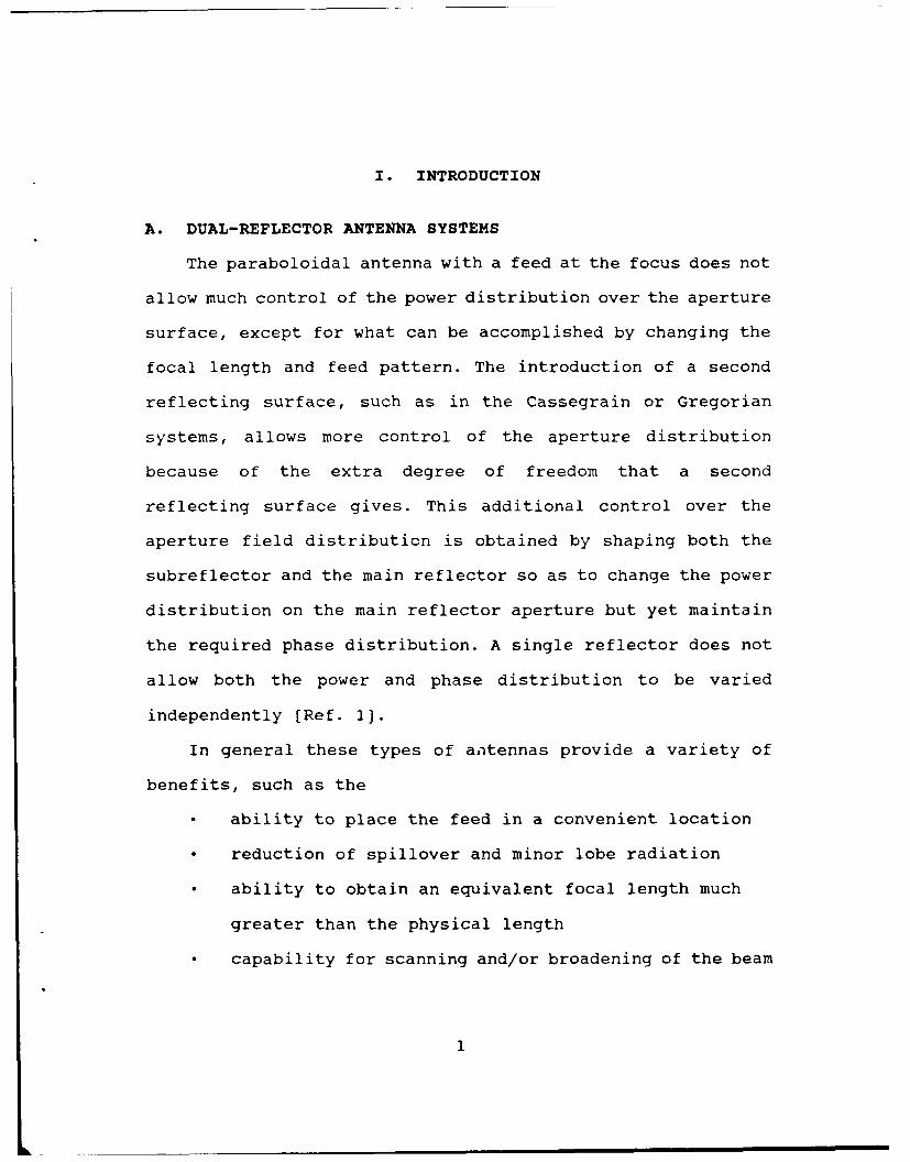
The Cassegrain antenna, which is shown in Figure 1 and

derived from telescope design [Ref. 3], is the most

common antenna using multiple reflectors. The feed illuminates

the hyperboloidal subreflector, which in turn illuminates the

paraboloidal main reflector. The feed is placed at one focus

of the hyperboloid and the paraboloid focus at the other. A

similar system is the Gregorian, which uses an ellipsoidal

subreflector in place of the hyperboloid as shown in Figure 2.

Hyperbolod

Figure 1: CLASSICAL CASSEGRAIN

2

F eed B

f ___ Ehpsoid

Figure 2: CLASSICAL GREGORIAN

Aperture blocking can be large for these types of antennas. It

may be minimized by choosing the diameter of the subreflector

equal to that of the feed. This "minimum blocking condition"

is derived using geometrical optics and does not always give

good results for electrically small antennas.

In the general dual-reflerctor case, blockage can be

eliminated by either of two ways:

(1) offsetting both the feed and the subreflector

[Ref. 4] and

(2) displacing the main reflector and compensating for

the displacement by reorienting the subreflector.

In the latter case rotational symmetry is maintained.

3

B. DISPLACED AXIS DUAL-REFLECTOR ANTENNA SYSTEMS

Mobile satellite communication terminals require small

antennas with high aperture efficiencies. The Cassegrain and

Gregorian antenna types, which are simple and therefore

inexpensive, are generally not suitable for this purpose since

their subreflectors have a relatively large blocking area,

causing a reduction in gain. In other words, they have low

efficiency for the sizes of interest ( 20 to 30 wavelengths).

One method of reducing blockage, yet maintaining

rotational symmetry, is to displace the main reflector away

from the axis of symmetry and then adjust the subreflector so

that a plane wave front is achieved in the aperture plane. A

displaced-axis antenna with a subreflector that is a portion

of a hyperboloid will be called an ATH for short, and one with

elliptical based subreflector an ATE (or ADE). Geometrical

optics analysis of the ATE and ATH can be found in [Ref. 5].

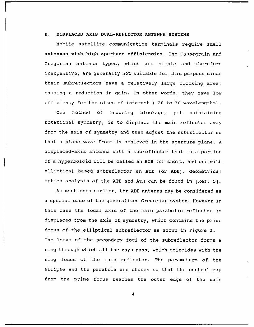
As mentioned earlier, the ADE antenna may be considered as

a special case of the generalized Gregorian system. However in

this case the focal axis of the main parabolic reflector is

displaced from the axis of symmetry, which contains the prime

focus of the elliptical subreflector as shown in Figure 3.

The locus of the secondary foci of the subreflector forms a

ring through which all the rays pass, which coincides with the

ring focus of the main reflector. The parameters of the

ellipse and the parabola are chosen so that the central ray

from the prime focus reaches the outer edge of the main

4

reflector, while the inner ray clears the outer edge of the

subreflector after reflection from the main reflector.

MAIN PARABO IC- OUTER RAYREFLECTOR -

PANG MAJOR AXISOF ELLIPSE

i FOCUS\ ,

" SUBREFL CTOR

P RIME D CISPLACED AXESFOCUS OF PARABOLA

INNER RAY -

Figure 3: DISPLACED AXIS ANTENNA (ADE)

The principal merits of this geometry are that the rays are

not reflected into the prime feed from the subreflector, nor

back into the subreflector from the main reflector. Also, the

aperture illumination for the radiated wave is more uniform

than that in tne standard Cassegrain or Gregorian

configuration. All rays reflected from the paraboloid miss the

subreflector, leading to a higher aperture efficiency. Another

advantage of the ADE antenna is that the F/D ratio of the main

reflector can be made smaller than that for a regular design,

leading to a compact antenna design with a reduction ini far-

out sidelobes [Ref. 6).

To summarize, the advantages of this type of design are

5

the main reflector may be made as small as ten

wavelengths while retaining a relatively high

efficiency

a low feed input reflection coefficient can be

achieved

small sidelobe and gain degradation due to aperture

blockage

elimination of the spares which normally hold the

subreflector (the subreflector can usually be

integrated into the feed design for small antennas).

subrefiectors which can be several times smaller than

those in Cassegrain antennas.

C. SCOPE OF THE STUDY

Chapter II discusses the derivation and the MM solution of

the electric field integral equation for a general body of

revolution (BOR) and measurements matrices are developed.

Chapter III discusses the MM solution for the ADE antenna

geometry and evaluates the excitation vector for an ideal

feed. Chapter IV explains the computer program that has been

devieloped based on an existing code written by Mautz and

Harrington. Chapter V discusses the results obtained by the

program and presents some guidelines for optimizing the

geometry. Chapter VI discusses conclusions based on the

results and presents some recommendations for further

research.

6

II. INTEGRAL EQUATIONS AND THE MOMENT METHOD

A. ELECTRIC FIELD INTEGRAL EQUATION

In the following analysis time-harmonic field quantities

are assumed. Phasor representations of the fields are used

with the eJWt time dependence suppressed.

The electric field integral equation (EFIE) is based on

the boundary condition that the total tangential electric

field on a perfectly electric conducting (PEC) surface of an

antenna or scatterer is zero. Then the total field E is the

sum of the incident and scattered fields. This can be

expressed as

(1)Etarn Etan + Ean = 0 on S

where S is the conducting surface of the antenna or scatterer.

The subscript 'tan' indicates tangential components. The

incident field that impinges on the surface S induces an

electric current density J., which in turn radiates the

scattered field.

The scattered field can be expressed in terms of a vector

potential A and a scalar potential # as

E (r) =-j(A - V (2)

where e -jkRA=IfJJ 4 rR ds7 (3)

R = Ir - r'I (4)

where r' is the point source location, and r is the

observation point location and

1 ff:. e-jkR ds (5)

The continuity equation relates the current and charge on the

surface v'Js =- (6)

or or i- V. (7)

Substitution of (3) and (7) into (2) gives the following

equation

ff, J.(. / e -jIR dS jVIVff s 'T -R:-(r)= S / jf -- V 7. e-jkR ds]

4nR e 41tR

(8)

This is the most general form of the EFIE. Let the free space

Green's function be denoted as

G(r,r') = e-jkR_ e-jkr-r'1 (9)47R 4 Ir-rI

so that (8) becomes

E 5 (r) =jw ff"J9 (rl) G(r,r') ds' + I -V[Vff J,(r) G(r,r') ds'

(10)

is only depends on the primed quantities and G is a scalar

that depends on both the primed and unprimed quantities. i_ is

the unknown quantity to be solved for.

8

For convinience, define an operator 9 which operates on is

~(J.) WGP ff, 47,(r') G (r, r) ds'+- V [ V fJ, (r') G (r, r') ds'

After using vector identities and modifying the last term

9 ,, jG pff J. (r') G (r, r') ds'+V [ff. VG (r, r') -J. (r') ds'I (12)

Since VG - V'G, where V' is defined with respect to the

source quantities,

ffVG(r, r') -J,(r')ds' ff, VG(rr') J.,(r) ds' (13)

Using vector identities and the surface divergence theorem, it

can be shown that

ffjw ) - V[(7-J.(r') ) G(r,r') ]dss C

(14)

The EFIE can now be written consisely as

g(L ) = • (15)

More detail on the development of the EFIE is available in

[Ref. 7] and in [Ref. 8].

B. SOLUTION OF THE EFIE USING THE METHOD OF MOMENTS

To solve (15) the method of moments is used. The method of

moments generates a generalized impedance matrix for the body

of interest. The excitation of the body is represented by a

voltage matrix, and the resultant current on the body is

9

represented by a current matrix [Ref. 2]. Equation (15) is

reduced to a matrix equation, which can then be solved using

standard methods.

The analysis and solution presented here are for the

special case of bodies which are rotationally symmetric about

an axis. Because of this symmetry a Fourier series expansion

in the angle of rotational symmetry reduces the problem to a

system of independent modes. This is important from the view

of computation; several small matrices must be inverted

instead of one large one.

The first step in the MM procedure is to expand Js into a

seriesJ. E ±j j (16)

j=1

where I. are the expansion coefficients to be determined and

the J- are called basis or expansion functions.

The J are usually chosen to be:

(1) consistent with the behavior of the actual ozuet

on the surface,

(2) mathematically convenient (i.e. have certain

desirable mathematical properties which will be

discussed later).

Equation (16) is substituted into (15), which, because of the

linearity of 9, becomes

0=Zt (17)

10

Similarity a set of N testing function (W,) is defined.

Although they need not be related to the set of basis

functions, they are usually chosen to be their complex

conjugate (Galerkin's Method). Now the inner product is

defined (W,J7>=f f W' Jds (18)

where W and J are tangential vectors on S. Taking the inner

product of both sides of the EFIE (equation (17))

(W,,(J)=(WE) i11, 2,3,....N . (19)

The subscript 'tan' has been dropped from Ei because the inner

product involves only tangential components. Now define

v.,(W 1 , E') (20)

Zij= (w,(J) (21)

so that (19) becomes

ZijI = Vi i =1, 2... N .(22)

Since there are N of these equations they can be written in

matrix form

[Z] [I] = [V] (23)

[Z] is the generalized impedance matrix and [V] is the

excitation vector. The vector of unknown current coefficients

can be solved for by inverting [Z]

11

[I] = [z]-'V[ ] = [Y [ V (24)

The impedance elements are

z = [f[w (jwAj+Vj)ds (25)S

If W is thought of as a current, the charge associated with it

is

(26)j6)

Now (25) can be written as

z1j =iff (W 1-A +pj'D ds (27)ff (2?)S

or or cIjr= f f r Ifjf -""j 1 'V (VWJ,)+ e kR (28)S (V '.W1 4 TER

where primed donates a source point (associated with J,) and

unprimed a field point (associated with Wj)

C. MM SOLUTION FOR THE SPECIAL CASE OF BODIES OF REVOLUTION

So far the discussion has been for an arbitrary conducting

body. In this section we restrict the surfaces to those

generated by revolving a plane curve about the z axis. Hence

an appropriate set of basis functions are

J, ct (t) einj * m=O, ±I, ±2 , . . 00 (29)

7--L = u f (t) ejl* m=0,±1,±2, .. ., (30)

12

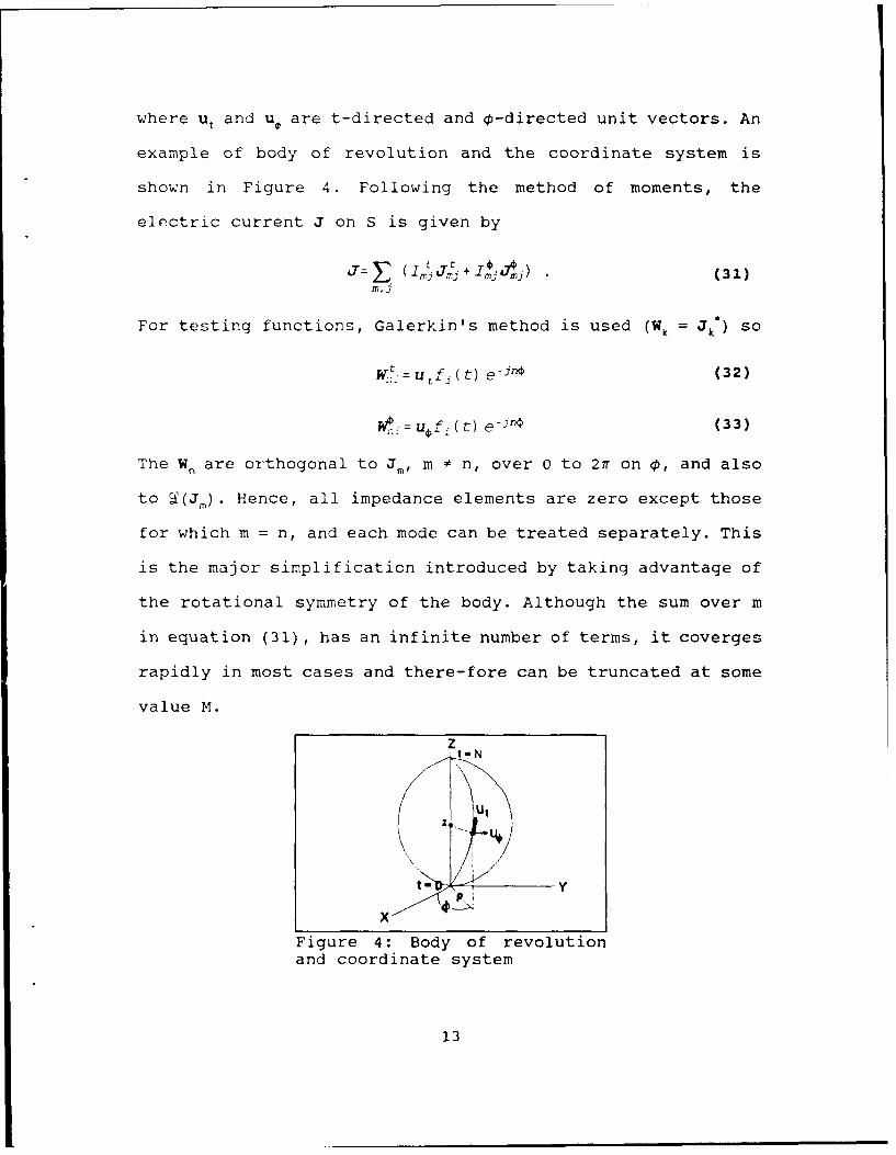
where ut and u. are t-directed and O-directed unit vectors. An

example of body of revolution and the coordinate system is

shown in Figure 4. Following the method of moments, the

electric current J on S is given by

,T (I"ffj M-7 + ImJ (31)MIj

For testing functions, Galerkin's method is used (Wk = Jk*) so

Kt .= U tfj (t) e - j l_ (32)

et" = uf4 (t) e - J (33)

The W, are orthogonal to JM, m * n, over 0 to 2r on p, and also

to V(Jm)- Hence, all impedance elements are zero except those

for which m = n, and each mode can be treated separately. This

is the major simplification introduced by taking advantage of

the rotational symmetry of the body. Although the sum over m

in equation (31), has an infinite number of terms, it coverges

rapidly in most cases and there-fore can be truncated at some

value M.

ZzUt

z

-YP,

Figure 4: Body of revolutionand coordinate system

13

The use of (29), (30), (32) and (33) to evaluate the

elements of (27) results in the matrix equation

[ZnII]~ i rit1 11' 1 V~t1]34Here the elements of the submatrices of Z are

(zt ij=(W ti, g (J~tj) >(Znl) (Wi U 170,) )(35)

(4) = J)

the elements of the submatrices V are

(Vnt ) i =(W', ') (36)

and the elements of the submatrices of I are the coefficients

in expansion (31). The solution to (34) can be written as

I = I IYt1 LY1I I CVr$2] (37)

The submatrices of Y are in general obtained after inversion

of the entire Z matrix, and not the inverses of the

corresponding Z submatrices. The -n mode matrices are related

to the +n mode matrices by

[y*t YII] [-Yet] r

Hence, only the n > 0 mode matrices need be inverted.

14

D. MEASUREMENT MATRICES

Obtaining the scattered field from the current J on the

body S can be done using a measurement vector

measurement = ff Er.Jds (39)

s

where Er is the plane wave field scattered by a differential

current element (a known function), which is weighted by the

current at every point on S. Since the current is given by

(31), (39) reduces to

measurement = [R] [I] (40)

where R is a measurement row vector

[R] = [(,j,Er)] (41)

and I is the current vector. Substitution of (24) into (40)

gives measurement = [R] [Y] [V] , (42)

For bodies of revolution, the expansion for J can be

separated into t- and O-directed components. Equation (41)

becomes (Rt) = ( 1 ,Er)

(43)

In partitioned form,

measurement R4[Rlt] [R (4~:1 [VJt (44)

15

A special case is that of the radiation field measurement.

Now the u-polarized scattered far-field from the current J on

S isE'u - -J e - j k R [R] [1) (45)4nR

where the elements of [R] are given by (43) with

El = ue-ikr (46)

This is a unit plane wave with polarization vector u and

propagation vector k. An arbitrary plane wave is a

superposition of two orthogonal components, for example E0 and

E.. Hence, (46) can be treated as two cases, one for u = u. and

the other for u = u.. To distinguish between the two cases let

(R =n) j (J ti, E ) (47 )

(R"') - (,7n ,oEj

for the 0-polarized case, and

(R$) t ( J41,E E( 48)n (48)E4NR > ni 4i,

for the 0-polarized case.

16

III. METHOD OF MOMENTS SOLUTION FOR THE ADE ANTENNA

A. CALCULATION OF IMPEDANCE ELEMENTS

The mathematical analysis in this section is based on

[Ref. 9:p 14-22] and [Ref. 10:p 3-18]. The expansion functions

Snjt and Jr' in equation (32), are chosen to be

C uT (t) j=1, 2, ... ,NP-2inI Ut p e n=0, ±1, ±2, ..... ±0' (9

UPj (t)e 4 j =1 2, ..,NP-I 50p1 n=O, ±1, ±2, . ... ±-

where: ut ,u, - unit vectors in the t and p direction

n - the mode number

p - the distance from the axis of symmetry to a point

on the body of revolution

pj - the value of p at t=t where t. is the center

point of the domain of the pulse

Tj(t) - triangle function shown in Figure 5, which

extends over segments j and j+l

Pj(t) - pulse function shown in Figure 6, which

extends only over a single segment j.

The purpose of the scale factor 1/pj is to give (50) the same

dimension as (49). The derivative of T,(t), which is shown in

Figure 8, is also required. The mathematical descriptions of

the functions are

17

AJ Ap , L 1 ( + ( t. ) + ( - + -- )) (52)

2 2/2

1, t- t j'-T,(t- 2 + (3)

1 t- t5 -

J3 (54)

S( t)

/ '

/

tj t. tU tJ~ t,2

Figure 5: Triangle function Tj(t)

Fj(t)

LL t0 tj . t

Figure 6: Pulse function Pj(t)

18

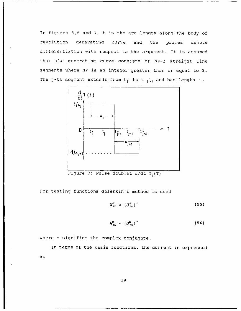
In Fig,:res 5,6 and 7, t is the arc length along the body of

revolution generating curve and the primes denote

differentiation with respect to the argument. It is assumed

that the generating curve consists of NP-i straight line

segments where NP is an integer greater than or equal to 3.

The j-th segment extends from t. to t - and has length *

dt

l /j I. .

i 1+1 j+1 J+2

0+1

Figure 7: Pulse doublet d/dt Tj(T)

For testing functions Galerkin's method is used

(-2 JEW) (55)

Wni ( n) (56)

where * signifies the complex conjugate.

In terms of the basis functions, the current is expressed

as

19

NP-2 NP- I

( IiJni* E IJ) . (57)n - i1i j1l

After applying the method of moments testing procedure a

matrix equation of the form of equation (25) results

I= Z-IV (58)

where

It Vt

1 1It Vt

2 V 2

t Z-1 Vt (59)

NP- 2 NP- 2

0 V

INP-i NP-i

I is the vector of current coefficients, V is the excitation

vector and Z is the method of moments impedance matrix.

The impedance matrix can be partitioned according to the

current and testing function components. For each azimuthal

mode .

Z = z, 40 t * (60)

For convenience let

20

MT = NP-2 ( number of surface triangles ) (61)

MP = NP-I ( number of surface pulses )

Thus the dimensions of the submatrices of Z are

Z tt - MTxMT

Z t- M MTxMP (62)

Znt . MPxMT

n "MPxMP

Althought n can take on values between ±o, the sum must be

truncated to some finite value, M. When multiple modes are

used, the complete impedance matrix becomes

Z_ 0 .......... 0

0 ............ . . 0

0 ............. . 0

Z= 0 ..... Zoss ..... 0 (63)

0 ... ... ... ... . . 00 .. .. .. ... .. .. . 0

0 ............ Z H

Fortunately this a block diagonal matrix; the inverse of Z is

also a block diagonal matrix with diagonal submatrices (Znss) 1.

To explicitly evaluate the impedance elements, the basis

and testing functions are used in equation (28)

Z .='-11 as a jR (J 'J q _ (V .T J) (Vs (64)

I 2

21

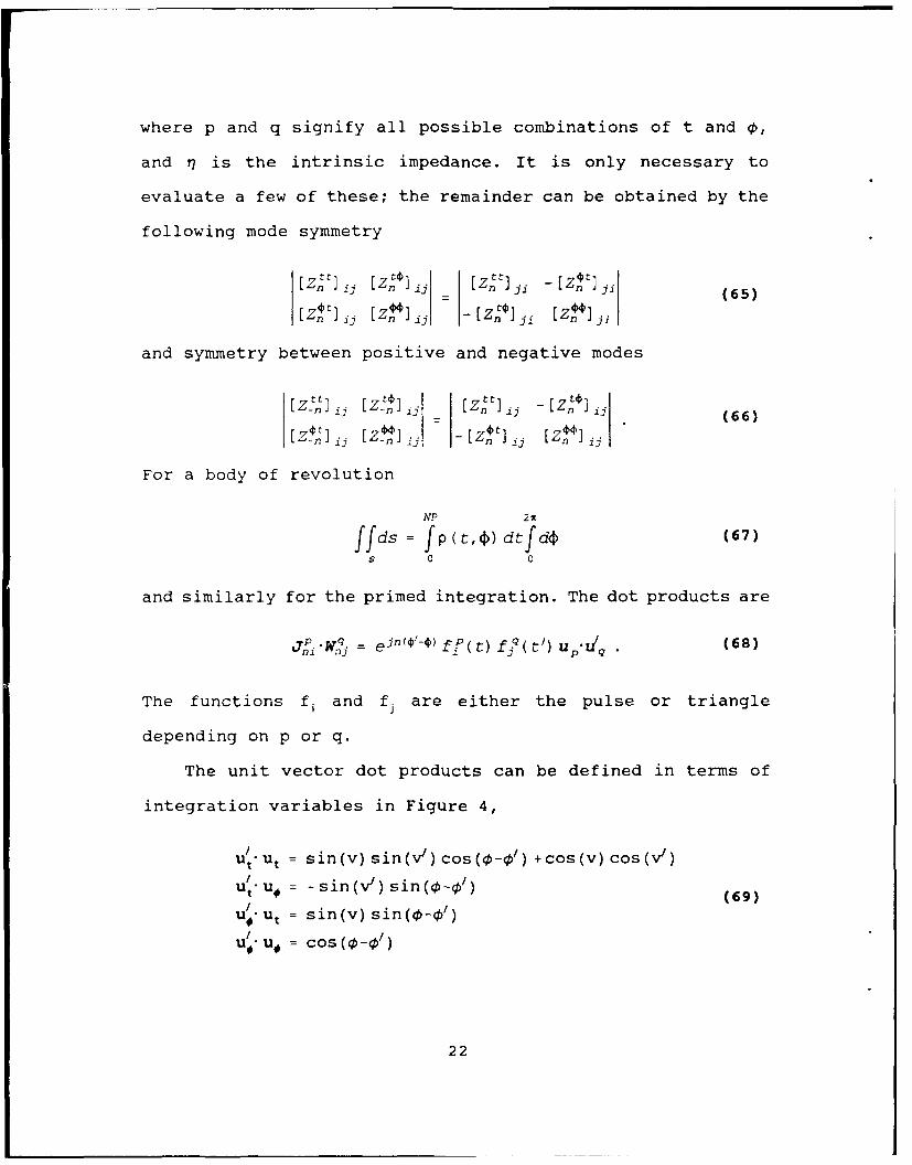
where p and q signify all possible combinations of t and (p,

and r7 is the intrinsic impedance. It is only necessary to

evaluate a few of these; the remainder can be obtained by the

following mode symmetry

Z t II ij I[Zn€7 I [Z ltlj -[zn ]Ji (65)

[Z!] ii [Zl ] - [zn] ; [zn] j

and symmetry between positive and negative modes

[Z" "°" [''li [For a body of revolution

NP 2x

ffds = f ) dtfd (67)S 0 0

and similarly for the primed integration. The dot products are

J k " q = e=in '- f f( t) fq( t') U U/q . (68)

The functions fi and f. are either the pulse or triangle

depending on p or q.

The unit vector dot products can be defined in terms of

integration variables in Figure 4,

ut'u t = sin(v) sin(v')cos(-/) +cos(v) cos(v')

Ut u* = -sin(v) sin(-/) (69)

UO'Ut = sin(v) sin(-1

0 u/. cos(1-0/)

22

Here v is the angle between the t direction and the Z-axis,

being positive if ut points away from the Z-axis and negative

if ut points toward it. Using equations (51), (52), (53) and

(54), the elements of Z are given by

t --

(Zn 1 j ifdt fdt'(kT (t) T, (t') (Gisin (v) sin W')(70)

+G3 cos (v)cos (v') G-I T,(t) -- /Tj(t'))3dt ' dt'

(z iJ= - f dPi 0 f dt'(kpT(t/)GxsinW)PI tj tj(71)

d+nG3 dt' % c'

tj 2 t7.1

(Znr) i -i fdt f dt'Pj(t') (kp'T (t) Gasin(v)Pj f -(72)t; t7

+ n G3 d- Tj ( t))+n3 dt

t 2. ITi. 1

(Zn -7J ~J f dt Pj<t) f dtP(t') (kpp'G-nG (73tj tj

where

Go = 2fdO--2e sin2(A) cos(n,) (74)J kR 2

0

Gi f d(-- -- os (() c s (n() (75)0

23

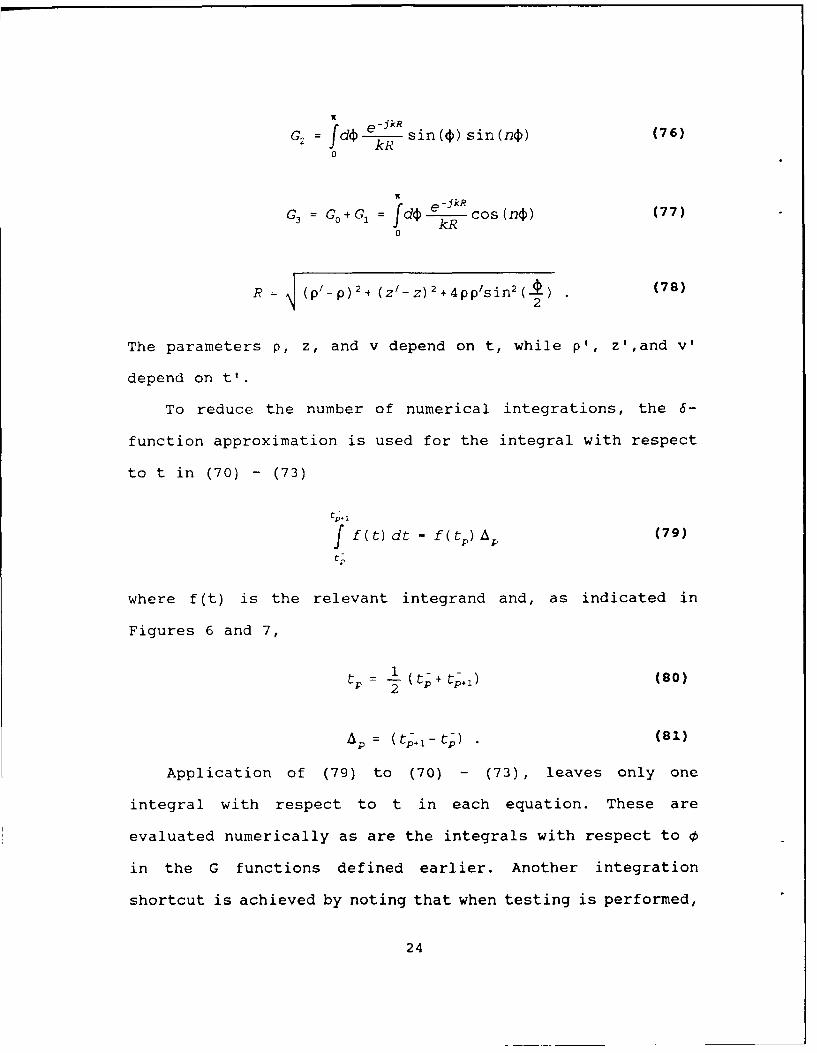
G = fd t sin(4) sin(n4) (76)

kR e jk0

G3 : Go+G f d4- cos(n@) (77)0

R = (p,_ Pp)2+ (z/,Z)2+4pp/sin 2(_) (78)2

The parameters p, z, and v depend on t, while p', z',and v'

depend on t'.

To reduce the number of numerical integrations, the 6-

function approximation is used for the integral with respect

to t in (70) - (73)

f f(t) dt - f (t) AP (79)

where f(t) is the relevant integrand and, as indicated in

Figures 6 and 7,

1P (t- + tP-.1) (80)

AP (tp+, - tp) (81)

Application of (79) to (70) - (73), leaves only one

integral with respect to t in each equation. These are

evaluated numerically as are the integrals with respect to (

in the G functions defined earlier. Another integration

shortcut is achieved by noting that when testing is performed,

24

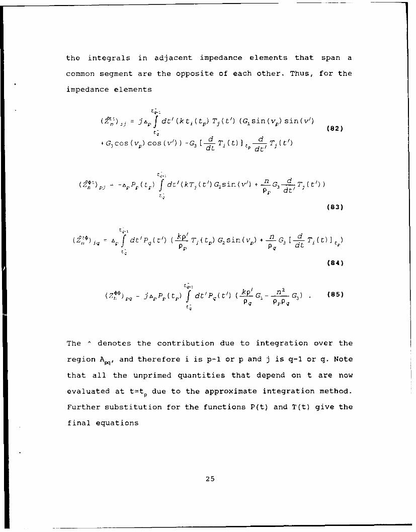
the integrals in adjacent impedance elements that span a

common segment are the opposite of each other. Thus, for the

impedance elements

Z n.) j Jp f d t ' (k t1 (tp) Tj W) (01 sin (vP) sin W )

(82)

+G3 cos(v)cos(v')) -G3 [Ti t d-'Ti(0dt L

(z"j)' ( -TP W(t)) T.(t')sin W ) + - - GpP P dt'T )tq

(83)

tq-

(Z ) (7= At , d tPI t) TL G s in vp) +-nG 3 [-Ti tP Pq YE

(84)

(Z : A j Pr(tp) f dt'Pqt') (--G- G3 ) (85)Pq P'Pq

tq

The ^ denotes the contribution due to integration over the

region A., and therefore i is p-l or p and j is q-1 or q. Note

that all the unprimed quantities that depend on t are now

evaluated at t=t due to the approximate integration method.

Further substitution for the functions P(t) and T(t) give the

final equations

25

8, G , n p S' (Vq) +G 3 cos (v) C05(v ))

+- (~)kp q (G lbsin (vp) sin (v,) + G3 bCOS (Vp) COS (Vq) (6

pi kApF qsin (vq) ) 2 q- AAsin(V7)G

p4 4 (87)

+ ( A G3a)2pp

(§4 (lA;A qs irn vp) ) (G~a s in (v,) G 2 ) + (- 1)~ 'nq) G3a

(88)

(Z") =2j k (Pq) (G1 & qSinl (Vq) G nq A) a P b) -2)q (2) 3a (89)

Gia 2 f G,~ ( t' - tq7) dt' m =0 , 1 , 2 (90)A

Gib 2 (-)2 f (t'- tq) G,(t' - t7) dt' m = 0,1,2 (91)

tQ

Substitution of Rpfor R in (75) - (77) gives

G0 tW- t) 2 fd e 'i (4 O n (92)

e ikRvG1 (t'-tq) = fd kR- c o s(4))c o s(n40) (93)

26

e-jkR

G(t - tq) f d4 sin(C) sin(n4) (94)0 kRp

where R is

RP= (pl_ p) I + (Z'- ZP) 2 + 42pmp'sin (9

Evaluation of the integrals in (92) through (94) is done

usina nt-point Gaussian quadrature

f -C cmf(am) (96)a JI

am b- ax+ b+ a (97)

2 2

where cm are the weights and xm are the zeros of the Legendre

polynomials. Typically nt = 2 is sufficient for the t-

integration. For the 0-integration the appropriate value

depends on the maximum radial extent of the surface. (An

approximate rule of thumb is 10 points per wavelength of

circumference.) The calculated values of Gm are substituted

into (92) and (93) in order to evaluate Gm and G. The

resulting values of G. and G are then substituted into (86)

- (89) to evaluate the elements of the impedance matrix.

The general MM solution can be applied to multiple

detached surfaces as in the ADE antenna. The extension to

multiple surfaces is primarily a bookkeeping problem that

complicates the computer code. A simple way of calculating the

27

current on multiple bodies is to perform the calculation as if

they were attached and then set the appropriate impedance and

excitation elements to zero.

Figure 8 shows the two reflector surfaces of the ADE

antenna connected by a fictitious "dummy segment." After the

Z-matrix calculation, any element that spans the m th segment

is set to zero, as shown in Figure 9 for the case of

triangular basis functions and Figure 10 for pulses.

m

\ dumny segment

NP

- Zm+l

Figure 8: ADE multiple surfaces

- rO v w.!V'4V, W

Figure 9: Triangle segments T, (t)

To avoid a singular matrix the diagonals of the zeroed rows

and columns are set to 1. The final matrix structure is

28

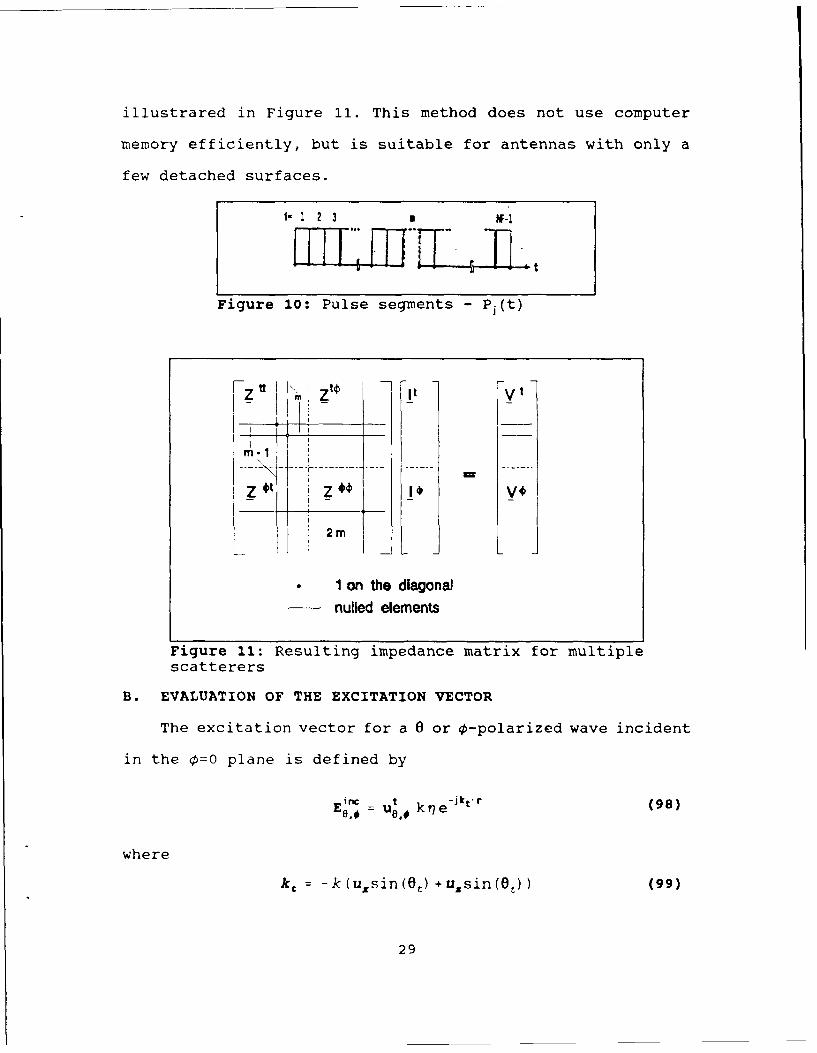
illustrared in Figure 11. This method does not use computer

memory efficiently, but is suitable for antennas with only a

few detached surfaces.

Figure 10: Pulse segments - Pj(t)

__ __ _ I t ___

m2m

1 on the diagonal

nulled elements

Figure 11: Resulting impedance matrix for multiple

scatterers

B. EVALUATION OF THE EXCITATION VECTOR

The excitation vector for a 0 or 0-polarized wave incident

in the 0=0 plane is defined by

En = t kt e-jkt'r (98)

where

k -k ( 2u.sin (9 ) + u.sin (0,) (99)

29

uO = Uy (100)

UO = Uxcos(ot) -uzsin(Ot) (101)

Ot is the angle of incidence and ux, uY, and u. are unit

vectors in the x, y, and z directions. r is the position

vector from the origin to the test point on the body. The

elements Vn t O are given by

v =i ffwi "E ds (102)'1S

A detailed development of the excitation vector can be found

in [Ref. 10: p 27-31]. The final results are obtained by

substituting (98) - (101) in (102). Using the same notation

developed earlier

Qt, j = jn7rk Ps in(vp) cos(0t) (Fn''a-Fn-l'a) - jn7rkApcos (vp) sin ((pt) F

+ (-1) p-i{ j 7rkApsin (vp) cos (0t) (Fflb-Ffllb)4

jnk7rkAPcos (vp) sin (0t)2 nb (103)

4,0 j t kpcos(Ot) ((F + , Asin (Fl +F

2 - ) +-" 2 pp ( 1,b n-1,b)

(104)

_ ((F -F_) + Fiv (FlbFnlb) i2 2 pp1

30

Vni -^jn k&PSi'n (v,,) (F ~ +F - - (-1) P-1j n k,&Psin V )

4 4"IFn,,b + Ff :.b)

(106)

New functions have been defined in (103) - (106),

Fa J, (kp sin (t) ) e-k cos(01)dt ; m=n-l,n,n l (107)A P -

Fm = 2__5 ( -t j) (kpsin(O :) ) eJZ° e dt ; m=n-l,n,n+1

(108)

Jm(kpsin(Ot)) is the m-th order Bessel function, which results

from the integration in (, and

p= pp4 (t-tp) sin(vP) (109)

z = + (t- tp) cos (vP) (110)

The remaining integrations are evaluated using a Gaussian

quadrature formula as in the case of the impedance elements.

At this point all of the quantities required to solve the

method of moments matrix equation have been defined. An

existing computer code, originally developed by Mautz and

Harrington, was modified to compute these elements for the ADE

antenna. The computer code operation is described in the

following chapter.

31

IV. COMPUTER PROGRAM

In this section, the FORTRAN program which implements the

numerical solution of CHAPTER III is discussed (the computer

listing is given in Appendix A). The program consists of a

MAIN PROGRAM and the subroutines ZMAT, SPHERE, PLANE, PLAN,

DECOMP, SOLVE and the functions BLOG, ETHETA, EPHI.

The main program obtains the radiation pattern and gain of

an ADE antenna for an ideal feed at body of revolution

coordinate system origin. The subroutine SPHERE calculates the

elements of excitation vector in (23) for spherical wave

incidence. The subroutine ZMAT calculates the elements of the

moment matrix in (24). The function BLOG is called by ZMAT.

The subroutines DECOMP and SOLVE solve the matrix equation

(24) for In"'. The subroutine PLANE calculates the plane wave

receive vector elements need to obtain the radiation field.

A. THE MAIN PROGRAM

The main program is divided to two main parts. The ADE

ANTENNA RADIATION PATTERN (lines 1 - 334) and the GAIN

PROGRAM(lines 335 - 453). Both parts are based on Mautz and

Harrington's computer program for bodies of revolution.

1. The ADE Antenna Radiation Pattern

This portion of the main program computes the

radiation pattern of an ADE type of antenna. An ideal feed (a

32

point source with a directive pattern) is at BOR coordinate

system origin and therefore only n = ±1 are required. Lines 17

- 73 are basic initializations including integration

coefficients for the 0-integration (NPHI) in lines 31 - 37,

and integration points for the t-integration (NT) in lines 43

- 48. The antenna geometry is defined in lines 49 - 59: the

total number of generating points (NP), the number of the main

reflector points (NPI) and the number of the subreflector

points (NP2). Lines 60 - 73 define the feed pattern which is

of the form

efd R (Gcos' (0) cos(.) + cos"(0) sin(4)) (111)

where n = FEXP and m = FHXP in the code. The simple case of a

Lambertian source is n,m = 1.

The next portion (74 - 211) of this part of the program

generates an array of surface contour pc~nts for calculating

the moment matrix and the excitation vector. Lines 74 - 113

define the antenna parameters which are discussed in Chapter

I. To create the Contour of the main reflector (which is

paraboloid), * is varied in the equation

= 2fRM = 2f -(112)1 + cos(W)

is the polar angle from the paraboloid vertex and R. is the

distamce from the focus to the surtace point at angle *. The

coordinates of the surface are

33

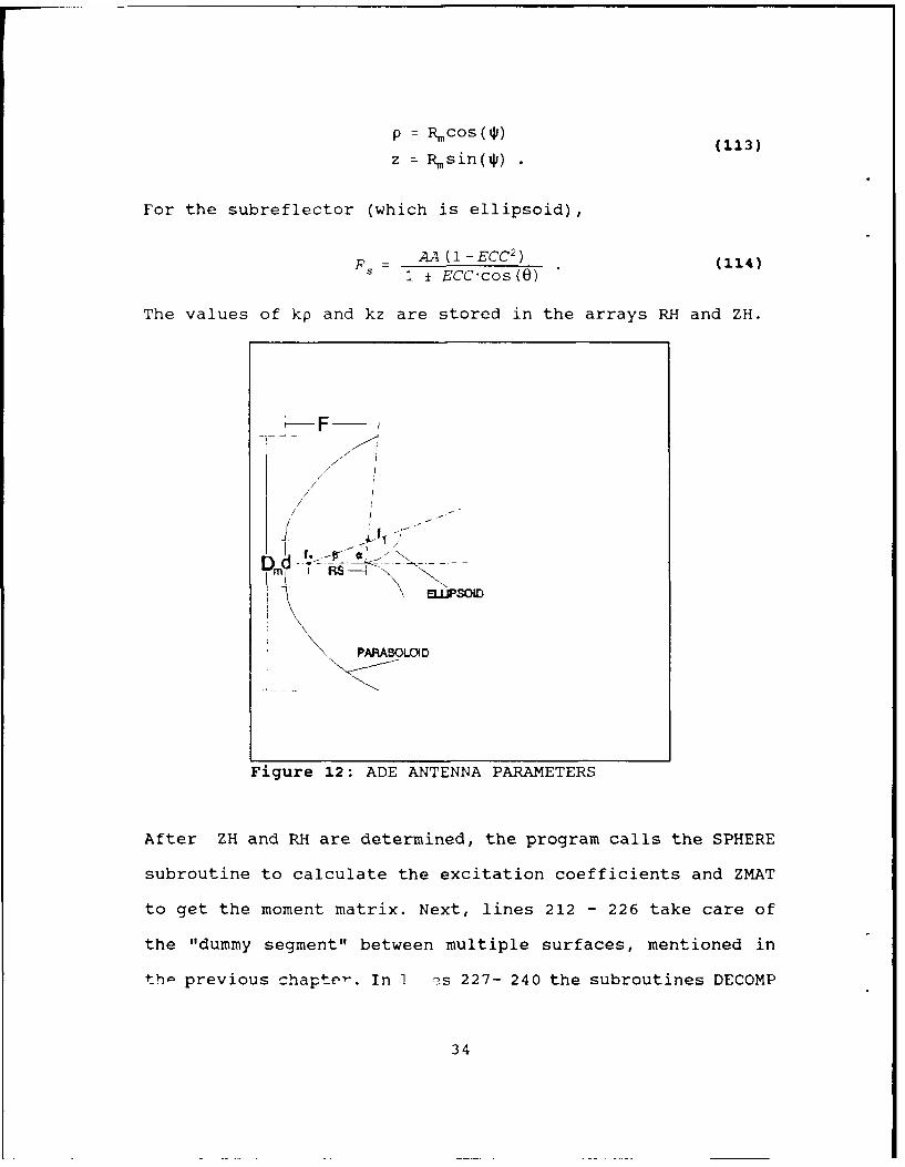
p = Rcos (*) (113)

z = Rsin(qi)

For the subreflector (which is ellipsoid),

S- AA (i-ECC2 ) (114)I± ECC'cos (0)

The values of kp and kz are stored in the arrays RH and ZH.

f ird

I/./ j -

I T

Rsv\

PARABOLOID

Figure 12: ADE ANTENNA PARAMETERS

After ZH and RH are determined, the program calls the SPHERE

subroutine to calculate the excitation coefficients and ZMAT

to get the moment matrix. Next, lines 212 - 226 take care of

the "dummy segment" between multiple surfaces, mentioned in

th- previous chaptev-. In I es 227- 240 the subroutines DECOMP

34

and SOLVE solve the ma- cix equation (24) for Int and In , and

in the lines 241 - 334 the far field patterns in the E and H

planes are computed according to equations (40) - (49).

2. Gain Program

The second half of the main program calculates the

gain and the efficiency of the ADE antenna. Far field pattern

integration, based on the previously calculated currents, are

used to get the total radiated power. Lines 315 - 360 are

initialization and specifying integration coefficientb for the

0 (NPHI) and t (NT) integrations. A normalization is loop

incorporated in lines 351 - 382 to obtain E. In lines 383 -

402 the 8 and 0-integration intervals are defined

The directivity is computed from the formula

27t n~

A ff IEe 1,( j2 R 2 SIN(O) Qjd( (115)00

DIRECTIVITY = Q -- (116)

where E(0,0) is the total electric field (i.e., that radiated

by the feed plus that scattered from the reflector). Ema is

obtained from the normalization loop.

B. THE SUBROUTINE SPHERE

The subroutine SPHERE computes the spherical wave

excitation vector for the body of revolution. The source is

assumed to be located at the origin of the BOR coordinate

35

system. The arguments are defined in the program. It returns

R, a column vector of length N containing Vt and V. for mode

n = +1, in that order.

C. THE SUBROUTINE ZMAT

The subroutine ZMAT calculates the moment matrix in (23)

for n = 1 and stores them in Z, which is the only output

argument. The storage of the Zn submatrices in Z is as

follows:

(Zt) Z(i+N* (j-l) + NP-2)n (117)

(Z0)i jG Z(i+N* (j-l) + (NP-2) *N)

(Z) j C Z(i+N* (j-1) + (NP-2) *N+NP-2)

where N=2*NP-3. More details about the ZMAT subroutine can be

found in (Ref. 10: p. 43-563.

D. THE SUBROUTINES DECOMP AND SOLVE

The subroutines DECOMP and SOLVE solve a system of N

linear equation in N unknowns. The input to DECOMP consist of

N and the N by N matrix of coefficients on the left-hand side

of the matrix equation stored by columns in Z. The output from

DECOMP is IPS and Z. The output is fed into SOLVE. The rest of

the input to SOLVE consists of N and the column of

coefficients on the right-hand side of the matrix equation

stored in B. The solution to the matrix equation is in X.

Further details concerning DECOMP and SOLVE can be found in

[Ref. 13: p. 46 - 49].

36

E. THE SUBROUTINES PLANE AND PLAN

The subroutines PLAN and PLANE are essentially the same

and compute the plane wave receive and excitation vectors for

the BOR according to (103) - (106). They are stored in R which

is the only output argument. The rest of the arguments of

PLANE and PLAN are input arguments and have all been defined

previously, except NF which is always 1 as implemented here.

The receive vectors are returned in the following order: Rte,

RO, R"', RO. These subroutines were written by Mautz and

Harrington, and are described in detail in [Ref. 12: p. 57 -

62].

37

V. COMPUTED RESULTS

An evaluation of practical ADE antenna configurations has been

performed using the MM computer code. The main reflector

diameter was 6" at 44 GHZ (22.352 wavelength), which was

chosen the same as the M.I.T-LINCOLN Lab design [Ref. 6]. A

second fixed parameter was the focal length to main reflector

diameter ratio (FOD) which was 0.15. The displacement distance

from the axis of symmetry to inside edge of the main reflector

is (d). The ratio of (d) to the main reflector diameter (dOD)

was fixed at 0.2. The edge angle of the paraboloid (ALPHA) is

equal to 105: The subreflector edge angle and the

eccentricity (or equivalently, the feed location, Rf) were

varied. The range of design parameters that was investigated

are summerized in Table 1. For each of these antennas the gain

was calculated. The gain was referred to that of a uniformly

illuminated unblocked aperture to arrive at an efficiency.

Because MM includes all of the interactions between the

surfaces, all of the loss mechanisms (edge diffractions,

surface waves, multiple reflections, etc.) are considered.

Only the feed is assumed to be ideal.

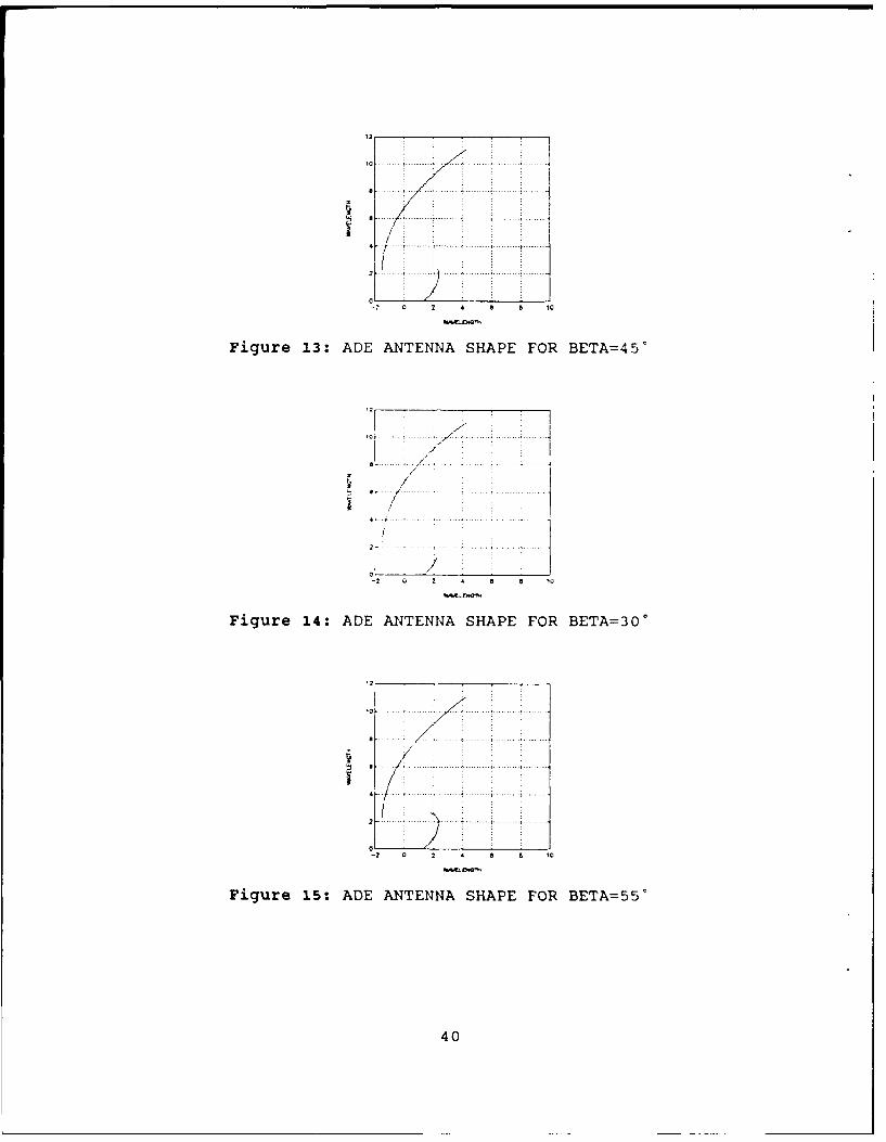
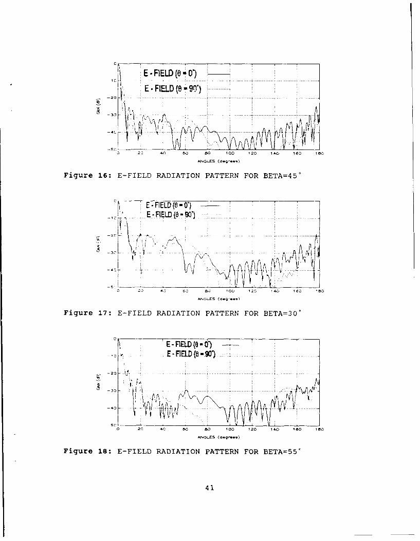
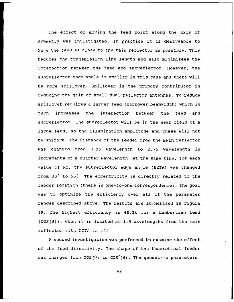
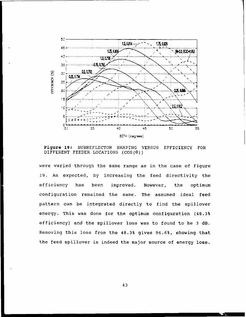
Three typical reflector configurations are shown in

Figures 13, 14, and 15. The principal plane patterns are given

in Figures 16, 17 and 18. The optimum occuitd for BETA = 45:

For smaller values of BETA the spillover increased. For larger

38

values of BETA the subreflector edge begins to turn back on

itself, which causes edge diffraction to increase and some

partial blocking of the wave reflected from the paraboloid.

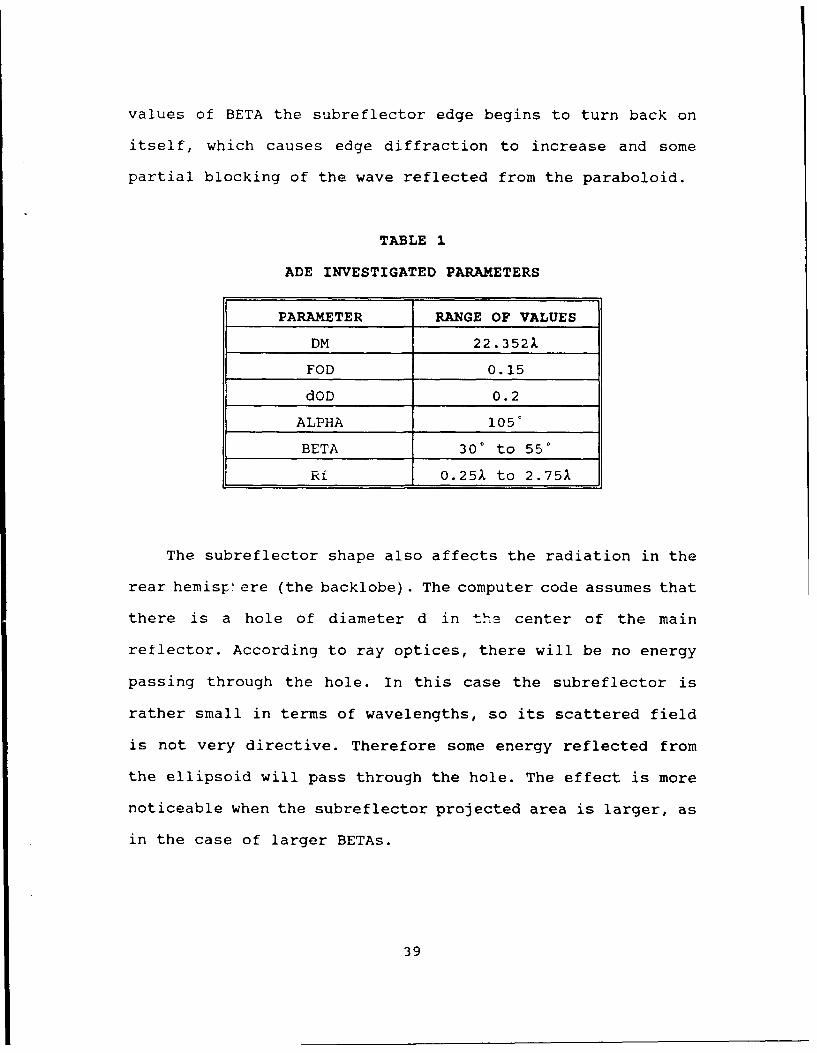
TABLE I

ADE INVESTIGATED PARAMETERS

PARAMETER RANGE OF VALUES

DM 22.3521

FOD 0.15

dOD 0.2

ALPHA 105'

BETA 30' to 55'

Rf 0.251 to 2.751

The subreflector shape also affects the radiation in the

rear hemisp: ere (the backlobe). The computer code assumes that

there is a hole of diameter d in th! center of the main

reflector. According to ray optices, there will be no energy

passing through the hole. In this case the subreflector is

rather small in terms of wavelengths, so its scattered field

is not very directive. Therefore some energy reflected from

the ellipsoid will pass through the hole. The effect is more

noticeable when the subreflector projected area is larger, as

in the case of larger BETAs.

39

24 4 5 1

-, 0 2 4 a 6 10

Figure 13: ADE ANTENNA SHAPE FOR BETA=5 0 *

04

-0

E -FIELD (0 0)

E E-FIELD (8 9)7 A

-5040o 60 80 10 120 160 18

Figure 17: E-FIELD RADIATION PATTERN FOR BETA=4O'

C!E E-ELDD(8 -)E-EDIE(S 9~

0 20 40 80o 10 12 4 160 180

ANGL-ES (aogruos)

Figure 18: E-FIELD RADIATION PATTERN FOR BETA=35*

E -RED 416

The effect of moving the feed point along the axis of

symmetry was investigated. In practice it is desireable to

have the feed as close to the main reflector as possible. This

reduces the transmission line length and also minimizees the

interaction between the feed and subreflector. However, the

subreflector edge angle is smaller in this case and there will

be more spillover. Spillover is the primary contributor in

reducing the gain of small dual reflector antennas. To reduce

spillover requires a larger feed (narrower beamwidth) which in

turn increases the interaction between the feed and

subreflector. The subreflector will be in the near field of a

large feed, so the illumination amplitude and phase will not

be uniform. The distance of the feeder from the main reflector

was changed from 0.25 wavelength to 2.75 wavelength in

increments of a quarter wavelength. At the same time, for each

value of Rf, the subreflector edge angle (BETA) was changed

from 300 to 55: The eccentricity is directly related to the

feeder location (there is one-to-one correspondence). The goal

was to optimize the efficiency over all of the parameter

ranges described above. The results are summerized in Figure

19. The highest efficiency is 48.3% for a Lambertian feed

(COS(O)), when it is located at 1.5 wavelengths from the mainrcf -Icctr wih nrTA - 45:

A second investigation was performed to examine the effect

of the feed directivity. The shape of the theoretical feeder

was changed from COS(O) to COS 2 (0). The geometric parameters

42

.. . ... ........... .. -... .. ...............................

........ ,.. .-... / ....

F .................... ................ .......... ... .. , ......, . ........... U 1.................... I .... ... ,-,.,.,,.. . ......... . ............... I ..... .- . ...... ........ ......... ,..... ... .-........... . / -.......

z 5 ...... .. ......... ........................ ... ..... ...... .......... i' ......... ..................................... 1 ...... .. .... ... .... ....... ,........ ..... ............. .... ........ .............. ......I7o* ............. 1

C. ' . : ... ...................... ................................. ... .......................... ....... ... .. ........ -'- - -

C- --- - -

3:. 40 45 5C 55

BE (degrees)

Figure 19: SUBREFLECTOR SHAPING VERSUS EFFICIENCY FORDIFFERENT FEEDER LOCATIONS (COS(O))

were varied through the same range as in the case of Figure

19. As expected, by increasing the feed directivity the

efficiency has been improved. However, the optimum

configuration remained the same. The assumed ideal feed

pattern can be integrated directly to find the spillover

energy. This was done for the optimum configuration (48.3%

efficiency) and the spillover loss was to found to be 3 dB.

Removing this loss from the 48.3% gives 96.6%, showing that

the feed spillover is indeed the major source of energy loss.

43

60~2 P1EL1

0AT 0.795ee

Fi ur 5 0 : U R F O S......................... VS.... ... .... ........ .... EF.C.E.. FOR ................

DIFF REN FE DE LO AT ON 0S.O,792(O))

44I

VI. SUMMARY AND CONCLUSIONS

In the previous chapters the EFIE was derived for

conducting surfaces and then specialized to multiple surfaces

of revolution with the ADE shape. A computer program was

written to solve for currents, far field radiation pattern,

gain and efficiency. Efficiency as a function of subreflector

shape (BETA) and the feeder location, was investigated for

various feed directivities.

The computed results that were obtained were predicable.

Maximum efficiency for an ideal source such as Lambertian was

48.3% for 6" diameter ADE antenna at 44 GHZ. The first

sidelobe level was -12 dB below the main beam. The second

sidelobe was -25 dB down at angle of 9' from the main lobe,

which is at the same location measured in [Ref. 6]. The

results show how the far-out sidelobes drop off rapidly, which

helps to reduce interference from outside sources which are

not located close to the main beam. The back lobe radiation

varies with the subreflector shape because of the hole at the

center of the main reflector. It is in the -25 dB range

relative to the main lobe which is typical for this small

reflector size. The efficiency of the ADE is higher than that

of a Cassegrain antenna of the same size and feed

illumination.

45

The computed and measured patterns for the configuration

of [Ref. 6] are for a dual band feed, which was not included

in the computed results. The program neglects feed

interactions with the reflector surfaces. In [Ref. 6.] a

circular waveguide is located very close to the subdish. Hence

the results are noticeably different for both the gain and

efficiency. However, it has been demonstrated that the program

gives an optimum point for the antenna geometry that is

relatively insensitive to the feed pattern. This provides a

starting point for the antenna design process. Once a

particular feed is selected, a development model can be built

and optimized by tuning the feed to minimize the feed and

subreflector interactions.

The next logical step is to include a more accurate feed

model into the antenna code so that the interactions between

it and the other surfaces are accounted for. Simple feeds can

be modeled directly; more complicated feeds can be simulated

using measured data. Since the suoreflector often lies in the

near field of the feed, a spherical wave expansion

representation of the measured feed field should be used.

The use of low-blockage feed types such as dipoles and

parasitic elements should be investigated. These types of

feeders will minimize the interaction between the feed and

subdish and can be included by slightly changing the program.

46

APPENDIX

COMPUTER CODES

1 C *ADE ANTENNA RADIATION PATTERN*2 C

C RADIATION PATTERN OF AN ADE ANTENNA4 C BASED ON MAUTZ AND HARRINGTON'S COMPUTER PROG FOR BORS.5 C SPHERICAL SOURCE IS AT BOR COORDINATE SYSTEM ORIGIN.6 C (THIS IMPLIES n=+1,-i ARE THE ONLY TWO NONZERO MODES.)7 C VARIABLE FEED EXPONENT; GAIN AND SPILLOVER LOSS ARE8 C COMPUTED9 C

10 C ICALC=O CALC CURRENTS AND FIELD11 C =1 CALC FIELDS ONLY (READ CURRENTS)12 C ICWRT=O WRITE CURRENTS )N DISC FILE13 C ISEG=O PRINT SURFACE SEGMENT POINTS14 C IPRINT=O PRINT TABLE OF FAR FIELD POINTS -- OTHERWISE ONLY15 C GAIN AND SPILLOVER ARE PRINTED16 C17 COMPLEX EP,ET,Z(300000),R(4000),B(2000),C(2000),U,UC18 COMPLEX ETT,EPT,ETST,ETSP,EPST,EPSP,EC,EX19 DIMENSION RH(2000),ZH(2000),XT(10),AT(10),IPS(500)20 DIMENSION AG(100),A(300),X(300),EXP(1200),ANG(1000)21 DIMENSION ECP(1000),XG(100),ECV(1000),EXV(1000)22 DIMENSION PHC(1000),PHX(1000),Q(30),S(30)23 DATA PI,START,STOP,DT/3.14159,0.,180.,I./24 DATA ICALC/O/,ISEG/O/,IPRINT/O/,ICWRT/O/25 DATA NT/2/,XT(1),AT(1)/.5773503,1./26 C DATA NT/4/,XT(1),XT(2),AT(1),AT(2)/.33998104,27 C *.8611363115,.6521451548,.3478548451/28 C29 C READ GAUSSIAN CONSTANTS30 C31 OPEN(1,FILE='/home/srvl/vered/thesis/outgaus',32 *STATUS='old')33 READ(1,*) NPHI34 DO 3 K=1,NPHI35 READ(1,*) X(K),A(K)36 3 CONTINUE37 CLOSE(1)38 RAD=PI,/180.39 BK=2.*PI40 U=(0.,l.)41 Uo=(0.,0.)42 UC=-U/4./PI43 NT2=NT/244 DO 1 K=1,NT2

47

1 KI=NT-K+12 AT (Kl) =AT (K)3 XT(K1)=XT(K)4 1 XT (K) =-XT (K)5 C6 C NP1=NU-MBER OF MAIN REFLECTOR PTS.; NP2=NUIMBER OF7 C SUBREFLECTOR PTS.8 C9 NP1=91

10 NP2=1911 NP=NP1+NP212 MP=NP-113 MT=MP-114 N=MT+MP15 write(6,*) 'npn=',np,n16 C17 C SPECIFY FEED PATTERN WHICH IN OUR CASE IS LAMBERTIAN WITH18 C N=I AND IS LOCATED AT THE ORIGIN.19 C20 C FEED FUNCTION EXPONENT:21 C ETHETA=COS (THETA) **FEXP*COS (PHI)22 C EPHI=COS (THETA) **FHXP*SIN(PHI)23 C24 FEXP=1.025 FE2=2.*FEXP+I.26 FHXP=1.027 FH2=2.*FHXP+1.28 DIR=2.*FE2*FH2/(FEXP+FHXP+1.)29 PRAD=1./FE2+1./FH230 C31 C READ THE ADE INPUT PARAMETERS:32 C33 C DM=MAIN REFLECTOR DIAMETER (PARABOLOID)34 C Rfeed=THE DISTANCE BETWEEN THE FEEDER AND THE MAIN REFLECTOR35 C36 C FOD=THE RATIO BETWEEN THE FOCUS AND THE DIAMETER OF THE MAIN37 C REFLECTOR38 C d/2=DISTANCE BETWEEN THE EDGE OF THE MAIN REFLECTOR AND THE39 C AXIS OF SYMMETRY40 C dOD=THE RATIO BETWEEN THE ABOVE d AND THE MAIN REFLECTOR41 C DIAMETER42 C ALPHA=THE ANGLE BETWEEN THE LOWER EDGE OF THE SUBREFLECTOR43 C TO THE SECOND FOCUS (NOT THE ORIGIN)44 C BETA=THE ANGLE BETWEEN THE AXIS OF SYMMETRY AND THE45 C IMAGINARY LINE BETWEEN THE ORIGIN TO THE EDGE OF THE46 C SUBREFLECTOR47 C ECC=ECCENTRICITY OF THE SUBREFLECTOR (ELLIPSOID)48 C49 C50 C FIRST GENERATE PARABOLOID CONTOUR51 C

48

1 WRITE(6,*) 'ENTER ALPHA'2 READ(5,*) ALPHA3 WRITE(6,*) 'ENTER BETA'4 READ(5,*) BETA5 WRITE(6,*) 'ENTER DM (IN WAVELENGTH)'6 READ(5,*) DM7 WRITE(6,*) 1FOD'8 READ(5,*) FOD9 WRITE(6,*) 'dOD'

10 READ(5,*) dOD11 ALPHA=ALPHA*RAD12 BETA=BETA*RAD13 FM=FOD*DM14 d~dOD*D415 Rmax=FM-d/2 ./TAN (P1-ALPHA)16 WRITE(6,*) 'MAXIMUM FEEDER DISTANCE IS', Rrnax17 WRITE(6,*) 'ENTER Rfeed (IN WAVELENGTH)'18 READ(5,*) Rfeed19 C20 C FM=FOCUS OF THE MAIN REFLECTOR (PARABOLOID)21 C ZSHIFT=INITIALIZE THE ORIGIN TO BE AT ZERO22 C23 ZSHIFT=FM-Rfeed24 DO 5 I=1,1;P125 TH=FLOAT(I-1) *ALPHA/FLOAT(NPl-1)26 RM=2.*FM/(l.+COS(TH))27 ZH(I)=(ZSHIFT-RM*COS(TH) )*BX28 RH(I)=(d/2.+RM*SIN(TH))*BK29 5 CONTINUE30 C31 C SUBREFLECTOR CONTOUR32 C33 PHIZ=ATAN(d/2./ZSHIFT)34 DELTA=PI -ALPHA-PHI Z35 CPZ=COS(PHIZ)36 CPS=COS(BETA)37 BB=2*SIN(DELTA)/SIN(ALPHA)38 AA=bb*COS(PHIZ)-139 ECC=(BB-SQRT(BB**2-4*(AA)) )/2/AA40 WRITE(6,*) 'ECCENTRICITY =',ECC41 EDGEE=CPS** (FEXP*2.)42 EDGEH=CPS**(FHXP*2.)43 EEDB=10.*ALOG1O(EDGEE)44 EHDB=1O.*ALOG1O(EDGEH)45 PSPILL=-FH2*(1.-EDGEE)+FE2*(1.-EDGEH)46 PSPILL=-PSPILL/ (FH2+FE2)47 PSDB=10.*ALOG1O(PSPILL)48 DO 6 I=1,NP249 THETA=FLOAT(I-1) *(BETA)/FLOAT(NP2-1)50 RSS=AA*((l.-ECC**2.)/(l.-ECC*COS(PHIZ-THETA)))*BK51 ZH(I+NP1)=RSS*COS(THETA)

49

1 RH(I+NP1)=RSS*SIN(THETA)2 6 CONTINUE3 OPEN(8, file='/home/srvl/vered/thesis/outADE')4 WRITE(8,8000) DM,RS,ECC,PHIZ/RAD,ALPHA/RAD,NP1,NP2,FEXP,5 * FHXP6 8000 FORMAT(//,5X,'*** ADE ANTENNA SYSTEM ***',//,5X,7 *'REFLECTOR PARAMETERS (LENGTHS IN WAVELENGTHS):',/,5X,8 *'IMAIN REFL DIA='I, F8. 3,/, 5X,'ISUB REFL DISTANCE='I,F8.3, /,9 *5X,'ECCENTRICITY=',F8.4,/,5X,'PHIZ (DEG)=',F8.2,/,5X,

10 * IALPHA (DEG)'=I, F8. 2,/, 5X, 'MAIN REFL POINTS (NPl) ='I,14,/11 *5X,'SUB REFL POINTS (NP2)=',I4,/,5X,'E-PLANE FEED12 *EXPONENT=',F8.3,/,5X,'H-PLANE FEED EXPONENT=',F8.3)13 WRITE(8,30) NT,NPHI14 30 FORMAT(/,7X,' NT NPHI',/,5X,15,2X,I5)15 IF(ISEG.EQ.0) WRITE(8,1300)16 1300 FORMAT(/,5X,'INDEX',8X,'Z(I)',1X,RHO(I)')17 OPEN(l,file='/home/srvl/vered/matlab/zeem.m')18 OPEN(2,file='/home/srvl/vered/matlab/rhom.n')19 OPEN(3,file='/hoxne/srvl/vered/matlab/zees.m')20 OPEN(4,file='/home/srvl/vered/matlab/rhos.m')21 DO 52 I=1,NP22 IF(ABS(ZH(I)).LT..001) ZH(I)=0.23 IF(ABS(RH(I)).LT..001) RH(I)=0.24 ZHB=ZH(I)/BK25 RH-B=RH(I)/BK26 IF(I.LE.NP1) THEN27 WRITE(1,31) ZHB28 WRITE(2,31) RHB29 ENDIF30 IF(I.GE.NP1+1) THEN31 WRITE(3,31) ZHB32 WRITE(4,31) RH-B33 ENDIF34 51 if(iseg.eq.0) WRITE(8,8004) I,ZHB,RHB35 52 CONTINUE36 8004 FORMAT(6X, 14,4X,F8. 3, 8X,F8.3)37 31 FORMAT(F8.4)38 CLOSE(1)39 CLOSE(2)40 CLOSE(3)41 CLOSE(4)42 write(6,*) 'geometry defined'43 IF(ICALC.EQ.1) THEN44 open(3, file='/home/srvl/vered/thesis/current')45 READ(3, *) DMO,DSO,FCO,PHIVO,PHIRO46 READ(3, *) ECCO,FODO,NP1O,NP2O,FEXPO,FHXPO47 WRITE(6, *) DMO,DSO,FCO,PHIVO,PHIRO,ECCO,FODO,NP1O,NP2O,48 *FEXPO49 WRITE(6, *) DM,DS,FC,PHIV,PHIR,ECC,FOD,NP1,NP2,FEXP50 READ(3,*) (RH(J),J=1,NP)51 READ(3,*) (ZH(J),J=1,NP)

50

1 READ(3,*) (C(J),J=1,N)2 WRITE(6,*) 'CURRENTS READ SUCCESSFULLY'3 CLOSE(3)4 ENDIF5 IF(ICALC.EQ.0) THEN6 CALL SPHERE (FEXP, FHXP,NP1,NP2 ,NT,RH, ZH, XT,AT, BK,R)7 DO 22 J=1,N8 B(J)==R(J)9 IF(J.GT.MT) B(J)=-B(J)

10 22 CONTINUE11 write(6,*) 'excitation coefficients computed'12 ENDIF13 CALL ZMAT(1, 1,NP1,NP2,NPHI,NT,RH,ZH,X,A,XT,AT,Z)14 write(6,*) 'back from zmat'15 C16 C NULL OUT ROWS AND COLUMNS CORRESPONDING TO DUMMY SEGMENTS17 C18 DO 700 LSS=l,N19 LS=LSS-120 Z(LS*N+NP1)=(0. ,0.)21 Z(LS*N+NP1-1)=(0. ,0.)22 700 Z(LS*N+NP1+MT)=(0.,0.)23 DO 701 LS=1,N24 Z((NP1-2)*N+LS)=(0. ,0.)25 Z( (NP1-1)*N+LS)=(0. ,0.)26 701 Z((NP1-1+MT)*N+LS)=(0.,0.)27 Z((NPl-2)*N+NP1-1)=(1. ,0.)28 Z ((NP1-1) *N+NP1)=(1., 0.)29 Z((MT+NP1-1)*N+NP1+MT)=(l.,0.)30 CALL DECOMP(N,IPS,Z)31 CALL SOLVE(N,IPS,Z,B,C)32 write(6,*) 'coefficients calculated'33 IF(ICWRT.EQ.0) THEN34 OPEN(3, file='/home/srvl/vered/thesis/current')35 WRITE(3, *) DM,DS,FC,PHIV,PHIR,ECC36 WRITE(3, *) FOD,NP1,NP2,FEXP,FHXP37 WRITE(3,*) (RH (J) ,J= 1,NP)38 WRITE(3,*) (ZH(J),J=1,NP)39 WRITE(3,*) (C(J),J=1,N)40 CLOSE(3)41 ENDIF42 991 CONTINUE43 IT=INT( (STOP-START) /DT)+144 C45 C RECEIVER PHI CUTS: DO 0 AND 90 (E- AND H- PLANES)46 C47 DO 400 IP=1,248 ECX=0.49 PHI=0.50 IF(IP.EQ.2) PHI=90.51 PHR=PHI*RAD

51

1 CNP=COS(PHR)2 SNP=SIN(PHR)3 DO 500 I=1,IT4 THETA=FLOAT(I-1) *DT+STARJT5 THX=THETA*RAD6 CALL PLANE(1, 1,NP1,NP2,NT,RH,ZH,XT,AT,THX,R)7 ETST=(0.,0.)8 EPST=(0.,0.)9 ETSP=(0.,0.)

10 EPSP=(0.,0.)11 DO 100 I0=1,MT12 ETST=ETST+R(I0)*C(I0)13 100 ETSP=ETSP+R(I0+N)*C(I0)14 DO 200 I0=1,MP15 EPST=EPST+R(I0+MT) *C(I0+MT)16 200 EPSP=EPSP+R(I0+N+MT) *C(I0+MT)17 ETF=CNP*FE (FEXP,THX)18 EPF=SNP*FH (FHXP, THX)19 ETT=2. *(ETST+EPST) *UC*CNP20 EPT=2.*J* (ETSP+EPSP) *UC*SNP21 ET=ETF+ETT22 EP=EPF+EPT23 EC= (ET*CNP-EP*SNP)24 EX= (ET*SNP+EP*CNP)25 ECV (I) =CABS (EC)26 EXV (I) =CABS (EX)27 ECR=REAL(EC)28 ECI=AIMAG(EC)29 EXR=REAL(EX)30 EXI=AIMAG(EX)31 PHC(I)=ATAN2 (ECI,ECR+1.e-10)/RAD32 PHX(I)=ATAN2 (EXI,EXR+1.e-10)/RAD33 ANG(I)=THETA34 ECX=AMAX1(ECX,ECV(I),EXV(I))35 500 CONTINUE36 IF(IP.EQ.1) THEN37 WRITE(8,103) ECX,EEDB,EHDB,PSPILL,PSDB38 103 FORMAT(/,5X,'E-PLANE EDGE TAPER=',F8.2,39 * /,5X,'H-PLANE EDGE TAPER=',F8.2,/,5X,'TOTAL PAD40 * POWER=',E15.5,41 * /,5X,'SPILLOVER LOSS =',F8.4,/,5X,' IN dB42 * =',f8.2)43 ENDIF44 WRITE(8,107) PHI45 107 FORMAT(/,5X,'PHI OF RECEIVER (DEG)=',F8.2)46 DO 600 I=1,IT47 ECP(I)=(ECV(I)/ECX)**248 EXP(I)=(EXV(I)/ECX)**249 ECP(I)=AMAX1(ECP(I),.00001)50 EXP(I)=AMAX1(EXP(I),.00001)51 ECP(I)=10.*ALOG1O(ECP(I))

52

1 EXP(I)=1O.*ALOG1O(EXP(I))2 600 CONTINUE3 IF(IPRINT.NE.0) GO TO 3004 WRITE(8,5015)5 5015 FORMAT(/,7X,'ANGLE',15X,'CO-POL',25X,'X-POL',/,7X,6 1'(DEG)1,4X,2('(VOLTS)',4X,'(DEG)1,3X,'(DB-REL)1,4X))7 DO 9000 L=1l,IT8 WRITE(8,5016)ANG(L),ECV(L),PHC(L),ECP(L),EXV(L),PHX(L)9 1,EXP(L)

10 5016 FORMAT(5X,F6.1,3X,2(F8.2,3X,F7.1,3X,F7.2,3X))11 9000 CONTINUE12 300 CONTINUE13 IF(IP.EQ.1) THEN14 OPEN(2, file='/home/srvl/vered/matlab/cang.m')15 OPEN(3,file='/home/srvl/vered/matlab/ccpole.m')16 OPEN(4,file='/hoxne/srvl/vered/matlab/cxpole.m')17 DO 9097 I=1,IT18 WRITE(2,5019) ANG(I)19 WRITE(3,5019) ECP(I)20 9097 WRITE(4,5019) EXP(I)21 CLOSE(2)22 CLOSE(3)23 CLOSE(4)24 ENDIF25 IF(IP.EQ.2) THEN26 OPEN(3,file='/home/srvl/vered/matlab/ccpolh.n')27 OPEN(4,file='/home/srvl/vered/matlab/cxpolh.m)28 DO 9098 I=1,IT29 WRITE(3,5019) ECP(I)30 9098 WRITE(4,5019) EXP(I)31 CLOSE(3)32 CLOSE(4)33 ENDIF34 400 CONTINUE35 5019 FORMAT(FS.3)36 C37 C program gain.f38 C39 C FAR FIELD PATTERN INTEGRATION FOR LOSS CALCULATIONS.40 C USES THE PREVIOUSLY CALCULATED CURRENTS TRANSFERRED FROM41 C pardip.f.42 C *** general wire/bor geometries can be handled43 C >>> INPUT FILE IS current44 C >>> HAS A GAIN NORMALIZATION LOOP INCORPORATED45 C46 OPEN(1, FILE= '/home/srvl/vered/thesis/outgaus')47 READ(1,*) NPHI48 NT2=NT/249 DO 7 K=1,NT250 K1=NT-K+151 AT(K1)=AT(K)

53

1 XT(Kl)=XT(K)2 7 XT (K) =-XT (K)3 DO 8 K=1,NPHI4 8 READ (1, *) XG (K),AG (K)5 NDIVT=16 NDIVP=17 S1=0.8 S2=180.9 Q1=0.

10 Q2=180.11 C12 C GAIN NORMALIZATION LOOP (USE THETA=PHI=0 AND THETA POL)13 C14 CNP=1.15 CALL PLAN(1,1,NP,NT,RH,ZH,XT,AT,0.,R)16 ETST=(0.,0.)17 EPST=(0.,0.)18 DO 101 I0=1,MT19 101 ETST=ETST+R(I0)*C(I0)20 DO 201 I0=1,MP21 201 EPST=EPST+R(IO+MT)*C(I0+MT)22 ETT=2 .* (ETST+EPST) *TC*CNP23 ETF=CNP*FE (FEXP, 0.)24 ET=ETT+ETF25 EMAX'=CABS(ET)26 WRITE(6,*) 'EMAX=',EMAX27 WRITE(8 ,8008) NT,NPHI ,NDIVP,NDIVT,S1,S2 ,Q1,Q228 8008 FORMAT(//,1OX,'NT=',I3,/,l0x,'NPHI=',I4,/,1OX,29 * 'NUMBER OF INTEGRATION INTERVALS IN PHI=',i3,/,l0x,30 * 'NUMBER OF INTEGRATION INTERVALS IN THETA=',i3,/,l0x,31 * 'THETA LIMITS: START,STOP=',F7.2,2X,F7.2,/,1OX,32 * 'PHI LIMITS: START,STOP=',F7.2,2X,F7.2)33 c34 c theta integration intervals35 c36 S1=Sl*RAD37 S2=S2*RAD38 Q1=Q1*RAD39 Q2=Q2*RAD40 DS=(S2-S1)/FLOAT(NDIVT)41 DO 502 I=1,NDIVT+142 S (I) =(I-1) *DS43 WRITE(6,*) "II,S(I)=",I,S(I)44 502 CONTINUE45 c46 c phi integration intervals47 c48 DQ=(Q2-Q1)/FLOAT(NDIVP)49 DO 503 I=l,NDIVP+150 Q(I)=(I-1)*DQ51 WRITE(6,*) "II,Q(I)=",I,Q(I)

54

1 503 CONTINUE2 SUM=0.3 do 2000 JJ=1,NDIVP4 Pl=DQ/2.5 P2=(Q(JJ+1)+Q(JJ))/2.6 DO 2000 J=1,NPHI7 PHR=pl*xg(j)+p28 DO 1000 II=1,NDIVT9 Tl=DS/2.

10 T2=(S(II+1)+S(II))/2.11 DO 1000 I=1,NPHI12 THR=T1*XG(I)+T213 IF(THR.LT.PI) GO TO 51014 THR=(BK-THR)15 PHR=PHR+PT16 510 CONTINUE17 SNP=SIN(PHR)18 CNP=COS(PHR)19 CALL PLAN(1, 1,NP,NT,RH,ZH,XT,AT,THR,R)20 STRA=SIN(THR)*AG(I)*AG(J)21 ETST=(0.,0.)22 EPST=(0.,0.)23 ETSP=(0.,0.)24 EPSP=(0.,0.)25 DO 104 I0=1,MT26 ETST=ETST+R(I0)*C(I0)27 104 ETSP=ETSP+R(10+N)*C(IO)28 DO 204 I0=1,MP29 EPST=EPST+R(I0+MT) *C(I0+MT)30 204 EPSP=EPSP+R(I0+N+MT) *C(I0+MT)31 ETT=2. *(ETST+EPST) *UC*CNP32 EPT=2.*13*(ETSP+EPSP) *UC*SNP33 ETF=CNP*FE (FEXP, THR)24 EPF=SNP*FH(FHXP,THR)

35 ET=ETT+ETF36 EP=EPT+EPF37 SUM=SUM+(CABS(ET)**2+CABS(EP)**2)*STRA38 1000 CONTINUE39 2000 CONTINUE40 PRAD=T1*P1*SUM41 GAIN=2.*PI*EMA1X**2/PRAD42 GDB=10.*aloglO(GAIN)43 EFF=GAIN/(PI*DM)**2.*100.44 WRITE (8,8010) PRAD, EMAX,GAIN,GDB,EFF45 8010 FORMAT(//,10X, 'TOTAL RADIATED POWER=',E15.8,/,1OX,46 * 'MAXIMUM FIELD VALUE (V/M)=',E15.8,/,1OX,47 * 'GAIN=',E15.8,/,l0x,'(dB)=',f8.2,48 * 'EFFICIENCY=',E15.8,2x,'%')49 WRITE(6,*)"PRAD,GAIN,dB=,EFFICIENCY",PRAD,GAIN,GDB,EFF50 32 FORMAT(F8.4)51 9999 STOP

55

1 END2 SUBROUTINE ZMAT(M1,M2,NP1,NP2,NPHI,NT,RH, ZH,X,A,XT,AT, Z)3 C4 C subroutine to compute the impedance elements for BORs.5 C original version from Mautz and Harrington (Improved E-Field6 C Method ... )7 C THE SUBROUTINE ZMAT CALLS THE FUNCTION BLOG8 C9 COMPLEX Ul,U2,U3,U4,U5,U6,U7,U8,U9,UA,UB,G4A(10) ,G5A(10)

10 COMPLEXG6A(10),G4B(10),G5B(10),G6B(1O),H4A,H5A,H6A,H4B11 COM!.EX CMPLX,H6B,UC,UD,GA(100),GB(100),H5B,Z(300000)12 DIME14SION RH(300),ZH(300),X(100),A(100),XT(10),AT(10)13 DIMENSION RS(300),ZS(300),D(300),DR(300),DZ(300)14 DIMENSION DM(300),C2(100),C3(100),R2(1O),Z2(10),R8(1O)15 DIMENSION C4(100),C5(100),C6(100),Z7(10),R7(10),Z8(10)16 NP=NP1+NP217 CT=2.18 CP=.119 DO 10 I=2,NP20 12=I121 RS(12)=.5*(RH(I)+RH(I2))22 ZS(12)=.5*(ZH(I)+ZH(I2))23 Dl=.5*(RH(I)-RH(I2))24 D2=.5*(ZH(I)-ZH(I2))25 D(12)=SQRT(Dl*Dl+D2*D2)26 DR(12)=Dl27 DZ(12)=D228 IF(RS(I2).EQ.0.) RS(12)=l.29 DM (12) =D(I2 )/RS (I2)30 10 CONTINUE31 M3=M2-M1+l32 M4=M1-133 P12=1.57079634 DO 11 K=1,NPHI35 PH=P12*(X(K)+l.)36 C2(K)=PH*PH37 SN=SIN(.5*PH)38 C3(K)=4.*SN*SN39 Al=P12*A(K)40 D4=.5*A1*C3(K)41 D5=A1*COS(PH)42 D6=A1*SIN(PH)43 M5=K44 DO 29 M=1,M345 PHM= (M4+M) *PH46 A2=COS(PHM)47 C4(M5)=D4*A248 C5(M5)=D5*A249 C6(M5)=D6*SIN(PHM)50 M5=M5+NPHI51 29 CONTINUE

56

1 11 CONTINUE2 MP=NP-13 MT=MP-1

*4 N=MT+MP5 N2N=MT*N6 N2=N*N7 U1=(O.,..5)8 U2=(O.,2.)9 JN=-1-N

10 DO 15 JQ=1,MP11 KQ=212 IF(JQ.EQ.1) 1(Q=l13 IF(JQ.EQ.MP) KQ=314 R1=RS(JQ)15 Z1=ZS(JQ)16 D1=D(JQ)17 D2=DR(JQ)18 D3=DZ(JQ)19 D4=D2/R120 D5=DM(JQ)21 SV=D2/D122 CV=D3/D123 T6=CT*Dl24 T62=T6+D125 T62=T62*T6226 R6=CP*R127 R62=R6*R628 DO 12 L=1l,NT29 R2(L)=R1+D2*XT(L)30 Z2(L)=Z1+D3*XT(L)31 12 CONTINUE32 U3=D2*U133 U4=D3*U134 DO 16 IP=1,MP35 R3=RS(IP)36 Z3=ZS(IP)37 R4=Rl-R338 Z4=Z1-Z339 FM=R4*SV+Z4*CV40 PHM=ABS(FM)41 PH=ABS(R4*CV-Z4*SV)42 D6=PH43 IF(Pf!M.LE.D1) GO TO 2644 D6=PHM-Dl45 D6=SQRT(D6*D6+PH*PH)46 26 IF(IP.EQ.JQ) GO TO 2747 KP=148 IF(T6.GT.D6) KP=249 IF(R6.GT.D6) KP=350 GO TO 2851 27 KP=4

57

1 28 GO TO (41,42,41,42),KP2 42 DO 40 L=1l,NT3 D7=R2(L)-R34 D8=Z2(L)-Z35 Z7(L)=D7*D7+D8*D86 R7(L)=R3*R2(L)7 Z8(L)=.25*Z7(L)8 R8(L)=.25*R7(L)9 40 CONTINUE

10 Z4=R4*R4+Z4*Z411 R4=R3*Rl12 R5=.5*R3*SV13 DO 33 K=1,NPHI14 Al=C3 (K)15 RR=Z4+R4*A116 UA=0.17 UB=0.18 IF(RR.LT.T62) GO TO 3419 DO 35 L=1l,NT20 R=SQRT(Z7(L)+R7(L)*Al)21 SN=-SIN(R)22 CS=COS(R)23 UC=AT(L)/R*CMPLX(CS,SN)24 UA=UA+UC25 UB=XT(L)*UC+UB26 35 CONTINUE27 GO TO 3628 34 DO 37 L--1,NT29 R=SQRT(Z8(L)+R8(L)*A1)30 SN=-SIN(R)31 CS=COS(R)32 UC=AT (L) /R*SN*CMPLX (-SN, CS)33 UA=UA+UC34 UB=XT(L)*UC+UB35 37 CONTINUE36 A2=FM+R5*A137 D9=RR-A2*A238 R=ABS(A2)39 D7=R-D140 D8=R+D141 D6=SQRT(D8*D8+D9)42 R=SQRT(D7*D7+D9)43 IF(D7.GE.0.) GO TO 3844 Al=ALOG( (D8+D6) *(-D7-~R)/D9)/D145 GO TO 3946 38 A1=ALOG((D8+D6)/(D7+R))/Dl47 39 UA=A1+UA48 UB=A2*(4./(D6+R)-A1)/D1+UB49 36 GA(K)=UA50 GB(K)=UB51 33 CONTINUE

58

1 1(1=02 DO 45 M=1,M33 H4A=0.4 H5A=0.5 H6A=0.6 H4B=0.7 H5IB=0.8 H6B=0.9 DO 46 K=1,NPHI

10 Kl=K1+111 D6=C4(KI)12 D7=C5(Kl)13 D8=C6(Kl)14 UA=GA(K)15 UB=GB(K)16 H4A=D6*UA+H4A17 H5A=D7*UA+H5A18 H6A=D8*UA+H6A19 H4B=D6*UB+H4B20 H5B=D7*UB+H5B21 H6B=D8*UB+H6B22 46 CONTINUE23 G4A(M)=H4A24 G5A(M)=H5A25 G6A(M)=H6A26 G4B(M)=H4B27 G5B(M)=H5B28 G6B(M)=H6B29 45 CONTINUE30 IF(KP.NE.4) GO TO 4731 A2=D1/(PI2*R1)32 D6=2./D133 D8=0.34 DO 63 K=1,NPHI35 Al=R4*C2 (K)36 R=R4*C3 (K)37 IF(R.LT.T62) GO TO 6438 D7=0.39 DO 65 L=1l,NT40 D7=D7+AT(L)/SQRT(Z7(L)+A1)41 65 CONTINUE42 GO TO6643 64 A1=A2/(X(K)+1.)44 D7=D6*ALOG(A1+SQRT(1.+A1*Al))45 66 D8=D8+A(K) *D746 63 CONTINUE47 A1=.5*A248 A?-L./A149 rj.=-P12*D8+2./Rl*(BLOG(A2)+A2*BLOG(Al))50 DO 67 M=1,M351 G5A(M)=D8+G5A(M)

59

1 67 CONTINUE2 GO0TO473 41 DO 25 M=1,M34 G4A(M)=O0.5 G5A(M)=0.6 G6A(M)=0.7 G4B(M)=0.8 G5B(M)=0.9 G6B(M)=0.

10 25 CONTINUE11 DO 13 L=1I,NT12 Al=R2(L)

13 R4=Al-R314 Z4=Z2(L)-Z315 Z4=R4*R4+Z4*Z416 R4=R3*A117 DO 17 K=1,NPHI18 R=SQRT(Z4+R4*C3 (K))19 SN=-SIN(R)20 CS=COS(R)21 GA(K)=CMPLX(CS,SN)/R22 17 CONTINUE23 D6=0.24 IF(R62.LE.Z4) GO TO 5125 DO 62 K=1,NPHI26 D6=D6+A(K)/SQRT(Z4+R4*C2 (K))27 62 CONTINUE28 Z4=3.141593/SQRT(Z4/R4)2? D6=-PI2*D6+ALOG(Z4+SQRT(1.+Z4*Z4))/SQRT(R4)30 51 Al=AT(L)31 A2=XT(L)*A132 K1=033 DO 30 M=1,M334 U5=0.35 U6=0.36 U7=0.37 DO 32 K=1,NPHI38 UA=GA(K)39 K1=K1+140 U5=C4 (Xl) *UA+U541 U6=C5(K1) *UA+U642 U7=C6(Kl) *UA+U743 32 CONTINUE44 U6=D6+U645 G4A(M)==A1*U5+G4A(M)46 G5A(M)=A1*U6+G5A(M)47 G6A(M)=A1*U7+G6A(M)48 G4B(M)=A2*U5+4B(lv:)49 G5B(M)==A2*U6+G5B(M)50 G6B(M)=A2*U7+G6B(M)51 30 CONTINUE

60

1 13 CONTINUE2 47 A1=DR(IP)3 UA=A1*U34 UB=DZ(IP)*U45 A2=D(IP)6 D6=-A2*D27 D7=Dl*Al8 D8=Dl*A29 JM=JN

10 DO 31 M=1,M311 FM=M44M12 Al=FM*DM(IP)13 H5A=G5A(M)14 H5B=G5B(M)15 H-4A=G4A(M)±H5A16 H4B=G4B(M)+H5B17 H6A=G6A(M)18 H6B=G6B(M)19 U7=UA*H5A+UB*H4A20 U8=UA*H5B+UB*H4B21 U5=U7-U822 U6=U7+Ug23 U7=-U1*H4A24 U8=D6*H6A25 U9=D6*H6B-A1*H4A26 UC=D7* (H6A+D4*H6B)27 UD=FM*JD5*114A

,e 8 Kl=IP+JM29 K2=K1+130 K3=K1+N31 K4=K2+N32 K5=1(2+MT33 K6=K4+MT34 K7=K3+N2N35 K8=K4+N2N36 GO TO (l8,2O,19),KQ37 18 Z(K6)=U8+U938 IF(IP.EQ.1) GO TO 2139 Z(K3)=Z(K3)-1U6-U740 Z(K7)=Z(1(7)+TUC-UD41 IF(IP.EQ.MP) GO TO 2242 21 Z(K4)-=U6±U743 Z (K8) =TJC+UD44 GO0TO2245 19 Z(K5)=Z(K5)+U8-U946 IF(IP.EQ.1) GO TO 23

4- Z(K1)=Z(R1)+U5+U'748 Z(K7)=Z(K7)+UC-UD49 IF(IP.EQ.MP) GO TO 2250 23 Z(K2)=Z(K2)iU5-U751 Z(K8)=UC+UD

61

1 GO TO 222 20 Z(K5)=Z(K5)+U8-U93 Z(K6)=U8+U94 IF(IP.EQ.1) GO TO 245 Z(K1)=Z(K1)+U5+U76 Z(K3)=Z(K3)4U6-U77 Z(K7)=Z(K7)+UC-UD8 IF(IP.EQ.MP) GO TO 229 24 Z(K2)=Z(K2)+U5-U7

10 Z(K4)=U6+U711 Z(Kg)=UC+UD12 22 Z(K8+MT)=U2*(D8*(H5A+D4*H5B)-A1*UD)13 JM=JM+N214 31 CONTINUE15 16 CONTINUE16 JN=JN+N17 15 CONTINUE18 DO 100 LSS=1,N19 LS=LSS-120 Z(LS*N+NP1)=(0.,0.)21 Z(LS*N+NP1-1)=(0. ,0.)22 100 Z (LS*N+NP1+MT) =(0. ,0.)23 DO 101 LS=1,N24 Z((NPl-2)*N+LS)=(0. ,0.)25 Z((NP1-1)*N+LS)=(0. ,0.)26 101 Z((NP1-1+MT)*N+LS)=(0.,0.)27 Z((NP1-2)*N+NP1-1)=(1. ,0.)28 Z((NP1-1)*N+NP1)=(1. ,0.)29 Z((MT+NP1-1)*N+NP1+MT)=(1.,0.)30 RETURN31 END32 SUBROUTINE SPHERE(FEXP,FHXP,NP1,NP2,NT,Ri, ZH,XT,AT,BK,R)33 C34 C SPHERICAL WAVE EXCITATION VECTOR - SOURCE ON Z AXIS35 C (r.=+1, -1 ONLY). DISTANCE BETWEEN ORIGINS (0 TO 0') IS ZF36 C37 COMPLEX R(2000),U,U2,U3,CEXP,PSI(300),F1E,F2E,F3E,F4E,38 COMPLEX CMPLX,UO,UES,UEC,UH,F1H, F2H39 DIMENSION TH(10),RII(300),ZH(300),XT(10),AT(10)40 NP=NP1+NP241 MP=NP-142 MT=MP-143 N=MT+MP44 U=(0.,1.)45 PI=3.14159346 P12=PI/2.47 DO 12 IP=1,MP48 K2=IP49 I=IP+15C1 DR=.5*(RH(I)-RH(IP))51 DZ=.5*(ZH(I)-ZH(IP))

62

1 D1=SQRT(DR*DR+DZ*DZ)2 Rl=.5*(RlH(I)+RH(IP))3 IF(ABS(Rl).LT.1.E-5) Rl~l.

*4 Z1=.5*(ZH(I)+ZH(IP))5 SVP=DR/D16 CVP=DZ/Dl

*7 DO 13 L=1l,NT8 QS=DR*XT(L)9 QC=DZ*XT(L)

10 TH(L)=ATAN2((R1+QS), (Z1+QC))11 RP=SQRT((Rl+QS)**2+(Zl+QC)**2)12 PSI(L)=CEXP(CMPLX(O.,-RP))/RP13 13 CONTINUE14 FlE=(0.,0.)15 F2E=(0.,O.)16 F3E=(0.,0.)17 F4E=(0.,0.)18 FlH=(0.,0.)19 F2H=(0.,0.)20 DO 15 L=1l,NT21 UO=AT(L)*PSI(L)22 UES=FE(FEXP,TH(L))*SIN(TH(L))*UO23 UEC=FE(FEXP,TH(L))*COS(TH(L))*UC24 UH=U0*FH(FHXP,TH(L))25 F1E=F1E+UES26 F2E=F2E+UEC27 F3E=F3E+UES*XT(L)28 F4E=F4E+UEC*XT (L)29 F1H=F1H+UH30 F2H=F2H+UH*XT(L)31 15 CONTINUE32 U2=-D1*PI2* (CVP*F1E-SVP*F2E)33 U3=-D1*P12* (CVP*F3E-SVP*F4E)34 K1=K2-135 R(K2+MT)=D1*U*PI* (F1H+D1*SVP*F2H/R1)36 IF(IP.EQ.1) GO TO 2137 R(K1)=R(K1)+U2-U338 IF(IP.EQ.MP) GO TO 2739 21 R(K2)=U2±U340 27 CONTINUE41 12 CONTINUE42 C43 C SIMPLIFIED METHOD FOR HANDLING MULTIPLE BODIES44 C46 R(NP1)=(O.,.)

47 R(NP1+MT)=(O.,O.)

48 RETURN49 END

* 50 SUBROUTINE SOLVE(N,IPS,UL,B,X)51 COMPLEX UL(300000),B(500),X(500),SUM

63

1 DIMENSION IPS(500)2 NP1=N+13 IP=IPS(1)4 X(1)=B(IP)5 DO 2 I=2,N6 IP=IPS(I)7 IPB=IP8 IM1=I-19 SUM=(0.,O.)

10 DO 1 J=l,IMl11 SUM=SUM+UL(IP)*X(J)12 1 IP=IP+N13 2 X(I)=B(IPB)-SUM14 K2=N* (N-i)15 IP=IPS (N) +K216 X (N) =X (N) /UL (I P)17 DO 4 IBACK=2,N18 I=NPl-IBACK19 K2=K2-N20 IPI=IPS (I) +K221 IP1=I+122 SUM=(0.,0.)23 IP=IPI24 DO 3 J=IP1,N25 IP=IP+N26 3 SU14=SUM+UL(IP)*X(J)27 4 X(I)=(X(I)-SUM)/UL(IPI)28 RETURN29 END30 SUBROUTINE DECOMP(N,IPS,UL)31 COMPLEX UL(300000),PIVOT,EM32 DIMENSION SCL(500),IPS(500)33 DO 5 I=1,N34 iPS(I)=I35 RN=0.36 Jl=I37 DO 2 J=1,N38 ULM=ABS(REAL(UL(J1)))+ABS(AIMAG(UL(J1)))39 J1=Jl+N40 IF(RN-ULM) 1,2,241 1 RN=ULM42 2 CONTINUE43 SCL(I)=1./RN44 5 CONTINUE45 NM1=N-146 K2=047 DO 17 K=1,NM148 BIG=O.49 DO 11 I=K,N50 IP=IPS(I)51 IPK=IP+4K2

64

1 SIZE=(ABS(REAL(UL(IPK)) )+ABS(AIMAG(UL(IPK) )) )*SCL(IP)2 IF(SIZE-BIG) 11,11,103 10 BIG=SIZE4 IPV=I5 11. CONTINUE6 IF(IPV-K) 14,15,147 14 J=IPS(K)8 IPS (K) =IPS (IPV)9 IPS(IPV)=J

10 15 KPP=IPS(K)+K211 PIVOT=:UL(KPP)12 KP1=K+113 DO 16 I=KP1,N14 KP=KPP15 IP=IPS(I)+K216 EM=-UL(IP)/PIVOT17 18 UL(IP)=-EM1s DO 16 J=KP1,N19 IP=IP+N20 KP=KP+N21 UL(IP)=UL(IP)+EM*UL(KP)22 16 CONTINUE23 K2=K2+N24 17 CONTINUE25 RETURN26 END27 FUNCTION BLOG(X)28 IF(X.GT. .1) GO TO 129 X2=X*X30 BLOG=((.075*X2-.1666667)*X2+1.)*X31 RETURN32 1 BLOG=ALOG(X+SQRT(1.+X*X))33 RETURN34 END35 FUNCTION FE(FEXP,X)36 P12=3.14159/2.37 FE=0.38 IF(ABS(X).LE.PI2) FE=ABS(COS(X))**FEXP39 RETURN40 END41 FUNCTION FH(FHXP,X)42 P12=3.14159/2.43 FH=0.44 IF(ABS(X) .LE.PI2) FH=-ABS(COS(X))**FHXP45 RETURN46 END47 SUBROUTINE PLANE(M1,M2 ,NP1,NP2,NT,RH, ZH,XT,AT,THR,R)48 C49 C Unchanged version from Mautz and Harrington report.50 C51 COMPLEX R(2000),U,U1,UA,UB,FA(10),FB(10),F2A,F2B,FlA,F1B

65

1 COMPLEX U2,U3,U4,U5,cnplx2 DIMENSION RH(300),ZH(300),XT(10),AT(10),R2(10),Z2(10)3 DIMENSION BJ(5000)4 NP=NP1+NP25 MP=NP-16 MT=MP-17 N=MT+MP8 N2=2*N9 CC=COS(THR)

10 SS=SIN(THR)11 11 CONTINUE12 U=(0.,1.)13 U1=3.141593*U**M114 M3=M1+l15 M4=M2+316 IF(M1.EQ.0) M3=217 M5=Ml+218 M6=M24-219 DO 12 IP=1,MP20 K2=IP21 I=IP+122 DR=. 5 *(R.H (I) -RHi(IP))23 DZ=.5*(ZH(I)-ZH(IP))24 D1=SQRT(DR*DR+DZ*DZ)25 Rl=.25*(RH-(I)+R}{(IP))26 IF(R1.EQ.0.) R1=1.27 Zl=.5*(ZH(I)+ZH(IP))28 DR=.5*DR29 D2=DR/R130 DO 13 L=1l,NT31 R2 (L)=R1+DR*XT(L)32 Z2(L)=Z1+DZ*XT(L)33 13 CONTINUE34 D3=DR*CC35 D4=-DZ*SS36 D5=D1*CC37 DO 23 M=M3,M438 FA(M)=O.39 FB(M)=0.40 23 CONTINUE41 DO 15 L=1l,NT42 X=SS*R2(L)43 IF(X.GT..5E-7) GO TO 1944 DO 20 M=M3,M445 BJ(M)=0.46 20 CONTINUE47 BJ(2)=1.48 5=1.49 GO TO 1850 19 M=2.8*X+14.-2./X51 IF(X.LT..5) M=11.8+ALOG1O(X)

66

1 IF(M.LT.M4) M=M42 BJ(M)=0.3 JM=M-1

*4 BJ(JM)=l.5 DO 16 J=4,M6 J2=JM7 JM=JM-18 J1=JM-19 BJ(JM) =Jl/X*BJ (J2) -BJ (JN±2)

10 16 CONTINUE11 S=0.12 IF(M.LE.4) GO TO 2413 DO 17 J=4,M,214 S=S+BJ(J)15 17 CONTINUE16 24 S=BJ (2) +2. *S17 18 ARG=Z2(L)*CC18 UA=AT(L)/S*CMPLX(COS(ARG) ,SIN(ARG))19 UB=XT(L)*UA20 DO 25 M=M3,M421 FA(M)=DJ(M) *UA+FA(M)22 FB(M)=BJ(M)*UB±FB(M)23 25 CONTINUE24 15 CONTINUE25 IF(Ml.NE.0) GO TO 2626 FA(1)=FA(3)27 FB(1)=FB(3)28 26 UA=Ul29 DO 27 M=M5,M630 M7=M-131 M8=M+132 F2A=UA*(FA(M8)+FA(M7))33 F2B=UA*(rB(M8)+FB(M7))34 UB=U*UA35 FlA=UB*(FA(M8)-FA(M7))36 F1B=UB*(FB(M8)-FB(M7))37 U4=D4*UA38 U2=D3*F1A+U4*FA(M)39 U3=D3*F1B+U4*FB(M)40 U4=DR*F2A41 U5=DR*F2B42 K1=K2-143 K4=KIL+N

44 K5=K2+N45 R(K2+MT)=-D5* (F2A+D2*F2B)46 R(K5+MT)=D1*(FlA+D2*FlB)

47 IF(IP.EQ.1) GO TO 2148 R(K1)=R(1(1)+U2-U:349 R(K4)=R(K4)+U4-U550 IF(IP.EQ.MP) GO TO 2251 21 R(K2)=U2+U3

67

1 R(K5)=U4+U52 22 K2=K2+N23 UA=UB4 27 CONTINUE5 12 CONTINIUF6 R(NP1-1)=(0.,0.)7 R (NPl) =(0. ,0. )8 R(NP1+MT)=(0.,0.)9 RETURN

10 END11 SUBROUTINE PLAN(M1,M2,NP,NT,RH, ZH,XT,AT,THR,R)12 C13 C PLANE WAVE RECEIVE VECTOR ELEMENTS. CAN BE USED TO COMPUTE14 C THE PLANE WAVE EXCITATION ELEMENTS IF PLANE WAVE SCATTERING15 C IS BEING CALCULATED. (THE RELATIONSHIP BETWEEN THE RECEIVE16 C AND EXCITAION ELEMENTS AS DISCUSSED BY MAUTZ AND17 C HARRINGTON.)18 C19 COMPLEX R(1800),U,U1,UA,UB,FA(5),FB(5),F2A,F2B,F1A,F1B20 COMPLEX U2,U3,U4,U5,CMPLX21 DIMENSION RH(1000),ZH(1000),XT(10),AT(10),R2(10)22 DIMENSION Z2(10),BJ(5000)23 MP=NP-124 MT=MP-125 N=MT+MP26 N2=2*N27 CC=COS(THR)28 SS=SIN(THR)29 U=(0.,1.)30 U1=3.141593*U**M131 M3=M1+132 M4=M2+333 IF(M1.EQ.0) M3=234 M5=M1+235 M6=M2+236 DO 12 IP=1,MP37 K2=IP38 I=IP+139 DR=.5*(RiH(I)-RH(IP))40 DZ=.5*(ZH(I)-ZH(IP))41 D1=SQRT(DR*DR+DZ*DZ)42 R1=.25*(RH(I)+RH(IP))43 IF(R1.EQ.0.) R1=1.44 Z1=.5*(ZH(I)+ZH(IP))45 DR=.5*DR46 D2=DR/R147 DO 13 L=1l,NT48 R2 (L)=R1+DR*XT(L)49 Z2(L)=Z1+DZ*XT(L)50 13 CONTINUE51 D3=DR*CC

68

1 D4=-.DZ*SS2 D5=Dl*CC3 DO 23 M=M3,M44 FA(M)=0.5 FB(M)=Q.6 23 CONTINUE7 DO 15 L=1l,NT8 X=SS*R2(L)9 IF(X.GT..5E-7) GO TO 19

10 DO 20 M=M3,M411 BJ(M)=0.12 20 CONTINUE13 BJ(2)=1.14 S=1.15 GO TO 1816 19 M=2.8*X+14.-2./X17 IF(X.LT..5) M=11.8+ALOGI0(X)18 IF(M.LT.M4) M=N419 BJ(M)=0.20 JM=M-121 BJ(JM)=l.22 DO 16 J=4,M23 J2=JM24 JM=JM-125 J1=JM-126 BJ(JM)=J1/X*BJ(J2)-BJ(JM42)27 16 CONTINUE28 S=o.29 IF(M.LE.4) GO TO 2430 DO 17 J=4,M,231 S=S±BJ(J)32 17 CONTINUE33 24 S=BJ (2)-4+2. *S34 18 ARG=Z2(L)*CC35 UA=AT(L)/S*CMPLX(COS(ARG) ,SIN(ARG))36 UB=XT(L)*UA37 DO 25 M=M3,M438 FA(M)=BJ(M)*UA+FA(M)39 FB(M) =BJ (M) *UB+FB(M)40 25 CONTINUE41 15 CONTINUE42 IF(M1.NE.0) GO TO 2643 FA(1)=FA(3)44 FB(1)=FB(3)45 26 UA=U146 DO 27 M=M5,M647 M7=M-148 M8=M+149 F2A=UA*(FA(M8)+FA(M7))50 F2B=UA*(FB(M8)+FB(M7))51 UB=U*UA

69

1 F1A=UB*(FA(M8)-FA(M7))2 F1B=UB*(FB(M8)-FB(M7))3 U4=D4*UA4 U2=D3*FlA+U4*FA(M)5 U3=D3*FlB+U4*FB(M)6 U4=DR*F2A7 U5=DR*F2B8 K1=K,2-19 K4=Kl+N

10 K5=K2+N11 R(K2+MT)=-D5*(F2A+D2*F2B)12 R(K5+MT)=D1*(FlA+D2*F1B)13 IF(IP.EQ.1) GO TO 2114 R(K1)=R(K1)+U2-U315 R(K4)=R(K4)4U4-U516 IF(IP.EQ.MP) GO TO 2217 21 R(K2)=U2+U318 R(K5)=U4+U519 22 K2=K2+N220 UA=UB21 27 CONTINUE22 12 CONTINUE23 RETURN24 END25

70

LIST OF REFERENCES

1. Collin, R. E., Antennas And Radiowave Propagation, pp.253-259, McGraw-Hill, 1985.

2. Skolnik, M. I., Radar Handbook, pp. 6.23-6.25, McGraw-Hill, 1990.

3. Hannan, P. W., Microwave Antennas Derived from theCassegrian Telescope, IRE Trans. Antennas Propagat., Vol. Ap-9, pp. 140-153, March 1961.

4. Balanis, C. A., Antenna Theory Analysis and Design, pp.637-642, John Wiley & Sons, Inc., 1982.

5. Yerukhhimovich, Y. A., "Analaysis of Two-Mirror Antennasof a General Type", Telecom. and Radio Engineering, Part 2,27, No. 11, pp. 97-103, 1972.

6. Rotman, W., and Lee, J. C., "Compact Dual-FrequencyReflector Antennas for EHF Mobile Satellite CommunicationTerminals," IEEE AP-S International Symposium Digest, II,Boston, Massachusetts, pp. 771-774, June 1984.

7. Balanis, C. A., Advanced Engineering Electromagnetic, pp.670-712, John Wiley & Sons, Inc., 1989.

8. Harrington, R. F., and Mautz, J. R., "Radiation AndScattering From Bodies Of Revolution, Final Rep., AFCRL-69-0305, Syracuse Univ., Syracuse, NY, July 1969.

9. Harrington, R. F., and Mautz, J. R., "H-FIELD, E-FIELD,AND COMBINED FIELD SOLUTION FOR BODIES OF REVOLUTION",TECHNICAL REPORT TR-77-2, SYracuse Univ., Syracuse, N.Y.,February 1977.

10. Harrington, R. F., and Mautz, J. R., " AN IMPROVED E-FIELDSOLUTION FOR A CONDUCTIVE BODY OF REVOLUTION ", TECHNICALREPORT TR-80-1, Syracuse Univ., Syracuse, N.Y., 1980.

71

INITIAL DISTRIBUTION LIST

1. Library, Code 52 2Naval Postgraduate SchoolMonterey, CA 93943-5002

2. Chairman, Code ECDepartment of Electrical and Computer EngineeringNaval Postgraduate SchoolMonterey, CA 93943-5002

3. Professor D. C. Jenn, Code EC/JnDepartment of Electrical and Computer EngineeringNaval Postgraduate SchoolMonterey, CA 93943-5002

4. Professor H. M. Lee, Code EC/LhDepartment of Electrical and Computer EngineeringNaval Postgraduate SchoolMonterey, CA 93943-5002

5. Aluizio Prata, Assistant ProfessorDepartment of Electrical EngineeringUniversity of Southern CaliforniaLos Angeles, CA 90089-0271

6. Defense Technical Information Center 2Cameron StationAlexandria, VA 22304-6145

7. Naval AttacheEmbassy of Israel3514 International Drive, N.W.Washington, D.C. 20008

8. The Head Of Electrical Division, Israeli NavyVia Naval AttacheEmbassy of Israel3514 International Drive, N.W.Washington, D.C. 20008

9. Vered Nissan 2Louis Marshal 7 StreetTel-Aviv, Zip Code: 62668Israel

72