method of measurement of capacitance and dielectric … · measurement science review, volume 15,...
TRANSCRIPT

MEASUREMENT SCIENCE REVIEW, Volume 15, No. 3, 2015
127
Method of Measurement of Capacitance and Dielectric Loss
Factor Using Artificial Neural Networks
Jerzy Roj, Adam Cichy 1Institute of Measurement Science, Electronics and Control, Silesian University of Technology, Gliwice, Poland,
[email protected], [email protected]
A novel method of dielectric loss factor measuring has been described. It is based on a quasi-balanced method for the
capacitance measurement. These AC circuits allow to measure only one component of the impedance. However, after analyzing a
quasi-balanced circuit's processing equation, it is possible to derive a novel method of dielectric loss factor measuring. Dielectric
loss factor can be calculated after detuning the circuit from its quasi-equilibrium state. There are two possible ways of measuring
the dielectric loss factor. In the first, the quasi-balancing of the circuit is necessary. However, it is possible to measure capacitance
of an object under test. In the second method, the capacitance cannot be measured. Use of an artificial neural network minimizes
errors of the loss factor determining. Simulations showed that the appropriate choice of the range of the detuning can minimize
errors as well.
Keywords: Dielectric loss factor, quasi-balanced circuits, artificial neural network.
1. INTRODUCTION
ANY PHYSICAL objects, which are dielectrics, can
be in a steady state modeled as a combination of RC
elements. Resistance R models the energy loss (so-
called active energy) and capacitance C models the energy
storage (so-called reactive energy). Such an object is, for
example, electrical insulation. An important parameter of
this model is the relationship between passive and active
energy of the tested object. This relationship is called the
dielectric loss factor. The phasor analysis of the object under
test also shows the name of tan δ because the loss factor is
the tangent of the phase angle, by which the phase shift
between current and voltage of the object is different from
the π/2 angle.
Dielectric loss factor is often measured in diagnostics of
electrical insulation. It is an indicator of insulation moisture
and allows the assessment of the degradation of the
insulation.
There are many methods of measuring the dielectric loss
factor used in practice. These are laboratory methods, such
as the calorimetric method, alternating current bridges (e.g.,
Schering bridge), algorithmic methods and other.
The measuring method is shown below, which, after the
modification and application of artificial neural network,
allows the measurement of dielectric loss factor.
2. MEASURING CIRCUIT
The measuring circuit shown in Fig.1. [1] is a
representative of a specific group of measuring circuits, the
so-called quasi-balanced circuits [2-10]. These circuits are
intended to measure AC impedance components. Their
special feature is to have a selected state, the so-called
quasi-equilibrium state.
Frequently, as in the circuit from Fig.1., this is the
orthogonality of the two selected signals. The circuit is
brought to this state by changes of a regulatory element. In
the circuit from Fig.1. it can be an adjustable gain of the
amplifier A or an adjustable conversion coefficient of the
current/voltage converter B.
Fig.1. Quasi-balanced circuit for capacitance measuring of an
object of RC type.
The measuring signals of the circuit from Fig.1., taking
into account that the phase shifter π/2 performs a
multiplication by the imaginary unit j, can be described as
follows:
XX IBVAw j1 ⋅−⋅= (1)
and
XIBw j2 ⋅= . (2)
As already mentioned, the circuit from Fig.1. has a state of
quasi-equilibrium which means orthogonality of w1 and w2.
This quasi-equilibrium state can be described by the
equation:
0Re2
1 =w
w. (3)
Because
M
10.1515/msr-2015-0019
MEASUREMENT SCIENCE REVIEW, Volume 15, No. 3, 2015
128
X
XX
IB
IBVA
w
w
j
j
2
1
⋅
⋅−⋅= (4)
and
X
XX
I
VZ = , (5)
so (3) can be written as follows:
1ImRe2
1 −= XZB
A
w
w. (6)
The equation determining the reactance of the serial object
under test is given as follows:
0
0ImA
BZ X = , (7)
where A0 and B0 are the voltage gain of the amplifier A and
the conversion rate of the current/voltage converter in the
quasi-equilibrium state, respectively.
Based on the reactance, the capacitance can be calculated
for object under test as follows:
0
0
B
ACX ω
= . (8)
As already mentioned, an adjustable gain of the amplifier
A or an adjustable conversion coefficient of the
current/voltage converter B can be used as a regulatory
element. More often an adjustable gain A is used, due to
simple calculations of the capacitance CX.
3. IDEA OF LOSS FACTOR MEASURING
The circuit from Fig.1. is suitable only for measuring of a
single impedance component. However, analysis of the
circuit shown below allows the use of such circuit to
measure the dielectric loss factor.
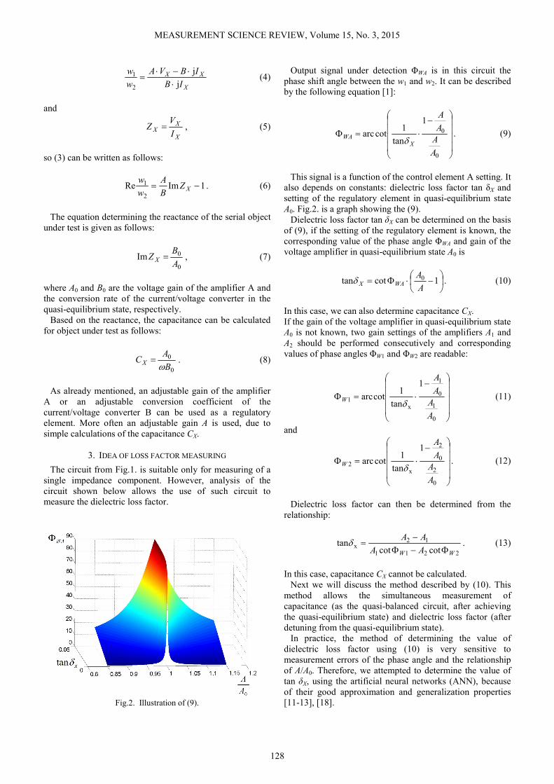
Fig.2. Illustration of (9).
Output signal under detection ΦWA is in this circuit the
phase shift angle between the w1 and w2. It can be described
by the following equation [1]:
−
⋅=Φ
0
0
1
tan
1cotarc
A
A
A
A
XWA δ
. (9)
This signal is a function of the control element A setting. It
also depends on constants: dielectric loss factor tan δX and
setting of the regulatory element in quasi-equilibrium state
A0. Fig.2. is a graph showing the (9).
Dielectric loss factor tan δX can be determined on the basis
of (9), if the setting of the regulatory element is known, the
corresponding value of the phase angle ΦWA and gain of the
voltage amplifier in quasi-equilibrium state A0 is
−⋅Φ= 1cottan 0
A
AWAXδ . (10)
In this case, we can also determine capacitance CX.
If the gain of the voltage amplifier in quasi-equilibrium state
A0 is not known, two gain settings of the amplifiers A1 and
A2 should be performed consecutively and corresponding
values of phase angles ΦW1 and ΦW2 are readable:
−
⋅=Φ
0
1
0
1
x1
1
tan
1cotarc
A
A
A
A
W δ (11)
and
−
⋅=Φ
0
2
0
2
x2
1
tan
1cotarc
A
A
A
A
W δ. (12)
Dielectric loss factor can then be determined from the
relationship:
2211
12x
cotcottan
WW AA
AA
Φ−Φ
−=δ . (13)
In this case, capacitance CX cannot be calculated.
Next we will discuss the method described by (10). This
method allows the simultaneous measurement of
capacitance (as the quasi-balanced circuit, after achieving
the quasi-equilibrium state) and dielectric loss factor (after
detuning from the quasi-equilibrium state).
In practice, the method of determining the value of
dielectric loss factor using (10) is very sensitive to
measurement errors of the phase angle and the relationship
of A/A0. Therefore, we attempted to determine the value of
tan δX, using the artificial neural networks (ANN), because
of their good approximation and generalization properties
[11-13], [18].
MEASUREMENT SCIENCE REVIEW, Volume 15, No. 3, 2015
129
4. SIMULATION
The study has been performed as a simulation, using the
library Neural Network Toolbox, available in the Matlab
environment [16]. The network with one hidden layer had
been implemented and then it was learned by the
Levenberg - Marquardt algorithm [17]. The sigmoid
activation function of neurons in the hidden layer [14], [15]
and a linear function in the output layer were used. The
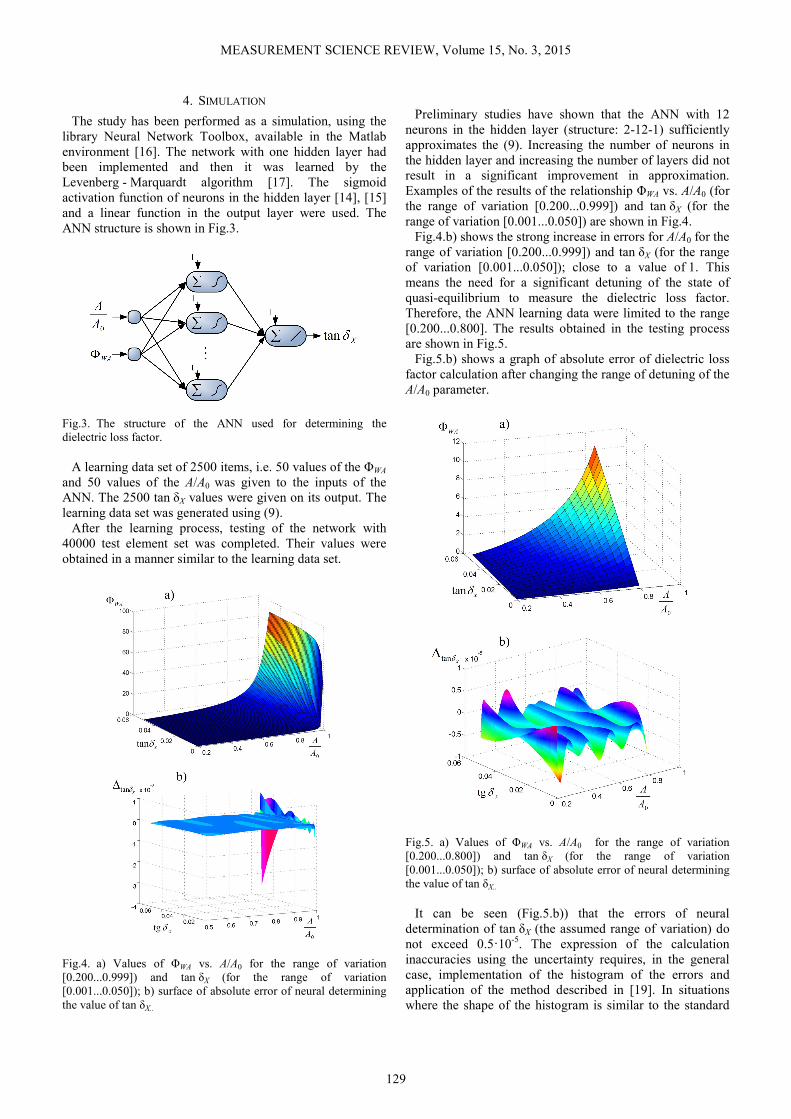
ANN structure is shown in Fig.3.
Fig.3. The structure of the ANN used for determining the
dielectric loss factor.
A learning data set of 2500 items, i.e. 50 values of the ΦWA
and 50 values of the A/A0 was given to the inputs of the
ANN. The 2500 tan δX values were given on its output. The
learning data set was generated using (9).
After the learning process, testing of the network with
40000 test element set was completed. Their values were
obtained in a manner similar to the learning data set.
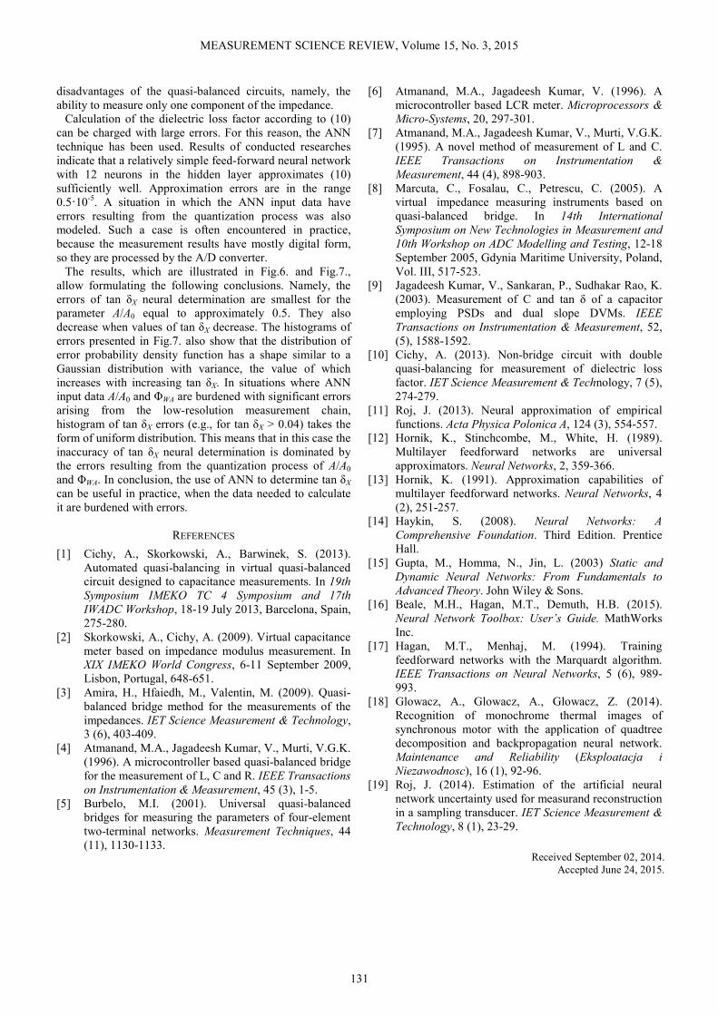
Fig.4. a) Values of ΦWA vs. A/A0 for the range of variation
[0.200...0.999]) and tan δX (for the range of variation
[0.001...0.050]); b) surface of absolute error of neural determining
the value of tan δX..
Preliminary studies have shown that the ANN with 12
neurons in the hidden layer (structure: 2-12-1) sufficiently
approximates the (9). Increasing the number of neurons in
the hidden layer and increasing the number of layers did not
result in a significant improvement in approximation.
Examples of the results of the relationship ΦWA vs. A/A0 (for
the range of variation [0.200...0.999]) and tan δX (for the
range of variation [0.001...0.050]) are shown in Fig.4.
Fig.4.b) shows the strong increase in errors for A/A0 for the
range of variation [0.200...0.999]) and tan δX (for the range
of variation [0.001...0.050]); close to a value of 1. This
means the need for a significant detuning of the state of
quasi-equilibrium to measure the dielectric loss factor.
Therefore, the ANN learning data were limited to the range
[0.200...0.800]. The results obtained in the testing process
are shown in Fig.5.
Fig.5.b) shows a graph of absolute error of dielectric loss
factor calculation after changing the range of detuning of the
A/A0 parameter.
Fig.5. a) Values of ΦWA vs. A/A0 for the range of variation
[0.200...0.800]) and tan δX (for the range of variation
[0.001...0.050]); b) surface of absolute error of neural determining
the value of tan δX..
It can be seen (Fig.5.b)) that the errors of neural
determination of tan δX (the assumed range of variation) do
not exceed 0.5·10-5
. The expression of the calculation
inaccuracies using the uncertainty requires, in the general
case, implementation of the histogram of the errors and
application of the method described in [19]. In situations
where the shape of the histogram is similar to the standard

MEASUREMENT SCIENCE REVIEW, Volume 15, No. 3, 2015
130
error probability density function (normal, uniform, etc.),
known statistical methods can be used.
However, note that the errors shown in Fig.5.b) relate to
an ideal situation, i.e. that the ΦWA and A/A0 values resulting
from (9) are given to the inputs of the neural network in the
testing process.
In practice, the ΦWA and A/A0 values are measurement
results, which are always obtained with a limited accuracy.
In order to model a situation of this kind, tests were carried
out for two cases. At first it was assumed that the A/A0 and
ΦWA values have errors arising from 12 and 8-bit
quantization, respectively. The assumption of such values is
justified by the typical measurement chain [19]. In the
second case it was assumed that both values are quantized
with low, 6-bit resolution.
The quantization process implemented by the A/D
converter was modeled using dependence:
+= 5.0 INT)(
q
xxnq , (14)
where x and nq(x) are quantities in the input and output of
the A/D converter, respectively, q is the quantum value,
INT(•) is a function which assigns the integer part of its
argument.
Fig.6. Surface of absolute error of neural determining of tan δX for
the A/A0 and ΦWA values quantized with a) 12-bit and 8-bit
resolution, respectively; b) 6-bit resolution both.
After performing a multiplication:
qxnx q ⋅= )(~ , (15)
relationship:
qxx ∆+= ~ (16)
is obtained, wherein Δq is a quantization error with uniform
distribution in the interval [-q/2, q/2]. The results of these
tests are shown in Fig.6.
It may be noted that the errors of neural determination of
tan δX are the smallest if the A/A0 ratio is detuned to
approximately 0.5 and it decreases with decreasing the value
of tan δX. Histograms of tan δX calculation errors for both
cases are shown in Fig.7.
Fig.7. Error histograms of neural tan δX calculation for the case of
a) Fig.6a; b) Fig.6.b).
Error histograms of neural tan δX calculation confirm
previous observations. Namely, for small values of tan δX
the histogram shape is similar to a Gaussian distribution
with a relatively small variance. With the tan δX increase
increases also the variance, while the shape of the histogram
is changed to resemble uniform distribution, as can be seen
especially in Fig.6.b).
5. CONCLUSION
The presented method of measuring of capacitance and
dielectric loss factor is based on a circuit implementing the
quasi-balanced method.
The capacitance of the object under test can be determined
knowing the values of control elements in the quasi-
equilibrium state. When detuning from the quasi-
equilibrium state, the dielectric loss factor can be
determined from (10). This eliminates one of the major
MEASUREMENT SCIENCE REVIEW, Volume 15, No. 3, 2015
131
disadvantages of the quasi-balanced circuits, namely, the
ability to measure only one component of the impedance.
Calculation of the dielectric loss factor according to (10)
can be charged with large errors. For this reason, the ANN
technique has been used. Results of conducted researches
indicate that a relatively simple feed-forward neural network
with 12 neurons in the hidden layer approximates (10)
sufficiently well. Approximation errors are in the range
0.5·10-5
. A situation in which the ANN input data have
errors resulting from the quantization process was also
modeled. Such a case is often encountered in practice,
because the measurement results have mostly digital form,
so they are processed by the A/D converter.
The results, which are illustrated in Fig.6. and Fig.7.,
allow formulating the following conclusions. Namely, the
errors of tan δX neural determination are smallest for the
parameter A/A0 equal to approximately 0.5. They also
decrease when values of tan δX decrease. The histograms of
errors presented in Fig.7. also show that the distribution of
error probability density function has a shape similar to a
Gaussian distribution with variance, the value of which
increases with increasing tan δX. In situations where ANN
input data A/A0 and ΦWA are burdened with significant errors
arising from the low-resolution measurement chain,
histogram of tan δX errors (e.g., for tan δX > 0.04) takes the
form of uniform distribution. This means that in this case the
inaccuracy of tan δX neural determination is dominated by
the errors resulting from the quantization process of A/A0
and ΦWA. In conclusion, the use of ANN to determine tan δX
can be useful in practice, when the data needed to calculate
it are burdened with errors.
REFERENCES
[1] Cichy, A., Skorkowski, A., Barwinek, S. (2013).
Automated quasi-balancing in virtual quasi-balanced
circuit designed to capacitance measurements. In 19th
Symposium IMEKO TC 4 Symposium and 17th
IWADC Workshop, 18-19 July 2013, Barcelona, Spain,
275-280.
[2] Skorkowski, A., Cichy, A. (2009). Virtual capacitance
meter based on impedance modulus measurement. In
XIX IMEKO World Congress, 6-11 September 2009,
Lisbon, Portugal, 648-651.
[3] Amira, H., Hfaiedh, M., Valentin, M. (2009). Quasi-
balanced bridge method for the measurements of the
impedances. IET Science Measurement & Technology,
3 (6), 403-409.
[4] Atmanand, M.A., Jagadeesh Kumar, V., Murti, V.G.K.
(1996). A microcontroller based quasi-balanced bridge
for the measurement of L, C and R. IEEE Transactions
on Instrumentation & Measurement, 45 (3), 1-5.
[5] Burbelo, M.I. (2001). Universal quasi-balanced
bridges for measuring the parameters of four-element
two-terminal networks. Measurement Techniques, 44
(11), 1130-1133.
[6] Atmanand, M.A., Jagadeesh Kumar, V. (1996). A
microcontroller based LCR meter. Microprocessors &
Micro-Systems, 20, 297-301.
[7] Atmanand, M.A., Jagadeesh Kumar, V., Murti, V.G.K.
(1995). A novel method of measurement of L and C.
IEEE Transactions on Instrumentation &
Measurement, 44 (4), 898-903.
[8] Marcuta, C., Fosalau, C., Petrescu, C. (2005). A
virtual impedance measuring instruments based on
quasi-balanced bridge. In 14th International
Symposium on New Technologies in Measurement and
10th Workshop on ADC Modelling and Testing, 12-18
September 2005, Gdynia Maritime University, Poland,
Vol. III, 517-523.
[9] Jagadeesh Kumar, V., Sankaran, P., Sudhakar Rao, K.
(2003). Measurement of C and tan δ of a capacitor
employing PSDs and dual slope DVMs. IEEE
Transactions on Instrumentation & Measurement, 52,
(5), 1588-1592.
[10] Cichy, A. (2013). Non-bridge circuit with double
quasi-balancing for measurement of dielectric loss
factor. IET Science Measurement & Technology, 7 (5),
274-279.
[11] Roj, J. (2013). Neural approximation of empirical
functions. Acta Physica Polonica A, 124 (3), 554-557.
[12] Hornik, K., Stinchcombe, M., White, H. (1989).
Multilayer feedforward networks are universal
approximators. Neural Networks, 2, 359-366.
[13] Hornik, K. (1991). Approximation capabilities of
multilayer feedforward networks. Neural Networks, 4
(2), 251-257.
[14] Haykin, S. (2008). Neural Networks: A
Comprehensive Foundation. Third Edition. Prentice
Hall.
[15] Gupta, M., Homma, N., Jin, L. (2003) Static and
Dynamic Neural Networks: From Fundamentals to
Advanced Theory. John Wiley & Sons.
[16] Beale, M.H., Hagan, M.T., Demuth, H.B. (2015).
Neural Network Toolbox: User’s Guide. MathWorks
Inc.
[17] Hagan, M.T., Menhaj, M. (1994). Training
feedforward networks with the Marquardt algorithm.
IEEE Transactions on Neural Networks, 5 (6), 989-
993.
[18] Glowacz, A., Glowacz, A., Glowacz, Z. (2014).
Recognition of monochrome thermal images of
synchronous motor with the application of quadtree
decomposition and backpropagation neural network.
Maintenance and Reliability (Eksploatacja i
Niezawodnosc), 16 (1), 92-96.
[19] Roj, J. (2014). Estimation of the artificial neural
network uncertainty used for measurand reconstruction
in a sampling transducer. IET Science Measurement &
Technology, 8 (1), 23-29.
Received September 02, 2014.
Accepted June 24, 2015.