methane emissions from three tropical hydroelectrical...
TRANSCRIPT

Methane emissions from three tropical hydroelectrical reservoirs
Emma Hällqvist
Arbetsgruppen för Tropisk Ekologi Minor Field Study 170 Committee of Tropical Ecology ISSN 1653-5634 Uppsala University, Sweden
Augusti 2012 Uppsala

Methane emissions from three tropical hydroelectrical reservoirs
Emma Hällqvist
Supervisors: Dr. Erik Sahlée, Department of Earth Sciences, Program for Air, Water and Landscape Sciences, Uppsala University, Sweden. Prof. Lars Tranvik, Department of Ecology and Genetics, Limnology, Uppsala University, Sweden. Dr. Luciano de Oliveira Vidal, Laboratory of Aquatic Ecology, Federal University of Juiz de Fora, Brazil. Prof. Fábio Roland, Laboratory of Aquatic Ecology, Federal University of Juiz de Fora, Brazil.

1
Abstract Freshwater systems are of great importance to the carbon cycle. When rivers are dammed to make the reservoirs needed for hydroelectricity, conditions are formed which generates greenhouse gas emissions to the atmosphere, and the question is raised weather hydropower is such a green source of energy as previously thought. The purpose of this study was to investigate CH4-fluxes from three tropical hydro-reservoirs; Funil, Santo Antônio and Três Marias, localized in Brazil with different trophic characteristics, carbon concentration, area and depth. Several samples were taken from different parts of the reservoirs to cover the spatial variation. To investigate CH4-emissions at the interface of air and water, floating static chambers were used. Concentrations were measured by gas chromatography (GC). The emission flow rate was estimated assessed by calculating the linear rate of gas accumulation in the chambers over time. The spatial variation of fluxes was very high in Santo Antônio, rangning from 0 to 39.6 mmol/m2/day. The variation appeared to depend on location in the reservoir, where higher emissions were found in tributaries, black water and downstream the dam. In Funil and Três Marias the fluxes were generally lower and ranging from 0-1 mmol/m2/day with slightly higher emissions seen in Funil. Two locations in Funil had higher fluxes (5.75 and 9.97mmol/m2/day). There was a negative trend between oxygen levels and CH4-fluxes between the reservoirs, with higher CH4-levels in the reservoir with the lowest oxygen concentration and vice versa. The trophic state and organic carbon-levels appeared to be important CH4 drivers in tropical Brazilian reservoirs.

2
Content Introduction ............................................................................................................................................. 4
Hydropower- an environmental debate .................................................................................. 4
Project background ................................................................................................................. 4
Main objectives ...................................................................................................................... 5
Hydropower- in Brazil and globally ....................................................................................... 6
The role of freshwater systems to greenhouse gas emission .................................................. 6
CO2- and CH4- production within reservoirs ........................................................................ 7
Flux pathways of CO2 and CH4 in reservoirs ......................................................................... 8
Important factors affecting the fluxes .................................................................................... 9
Material and Methods ............................................................................................................................ 11
Summary of procedure ......................................................................................................... 11
Preparation ........................................................................................................................... 12
Building the chambers ................................................................................................................... 12
Preparing the vials ......................................................................................................................... 12
Sampling procedure .............................................................................................................. 13
Fieldwork....................................................................................................................................... 13
CH4-sampling ............................................................................................................................... 13
Other sampling .............................................................................................................................. 14
GC-measurements ......................................................................................................................... 15
Study Areas .......................................................................................................................... 16
Funil .............................................................................................................................................. 16
Santo Antônio reservoir ................................................................................................................. 17
Três Marias .................................................................................................................................... 19
Calculations .......................................................................................................................... 20
Fundamentals: ............................................................................................................................... 20
Concentration of gas in initial water sample based on headspace extraction method ................... 21
The Flux calculated with a linear approach: .................................................................................. 21
Extrapolation of diffusive fluxes ................................................................................................... 22
Statistics ............................................................................................................................... 23
Results ................................................................................................................................................... 24
CH4- Concentrations and Fluxes .......................................................................................... 24
Initial samples ................................................................................................................................ 27
Emergent plant emissions .............................................................................................................. 28
CH4 vs. CO2 and O2 .............................................................................................................. 28
Profiles........................................................................................................................................... 30

3
Carbon and Nutrients ........................................................................................................... 31
Carbon ........................................................................................................................................... 31
Nutrients ........................................................................................................................................ 32
Variables ............................................................................................................................... 34
Discussion ............................................................................................................................................. 36
Fluxes and concentrations .................................................................................................... 36
Carbon and Nutrients ........................................................................................................... 36
Comparison between the reservoirs ............................................................................................... 36
The reservoirs ....................................................................................................................... 37
Funil .............................................................................................................................................. 37
Santo Antônio ................................................................................................................................ 38
Três Marias .................................................................................................................................... 40
Comparison to other studies ................................................................................................. 40
Variables ............................................................................................................................... 41
The importance of spatial and seasonable-variations ........................................................... 41
Sources of error .................................................................................................................... 42
External factors .............................................................................................................................. 42
Measurement techniques ............................................................................................................... 42
Conclusions .......................................................................................................................... 43
Thank you ............................................................................................................................. 43
References ............................................................................................................................ 44
4
Introduction
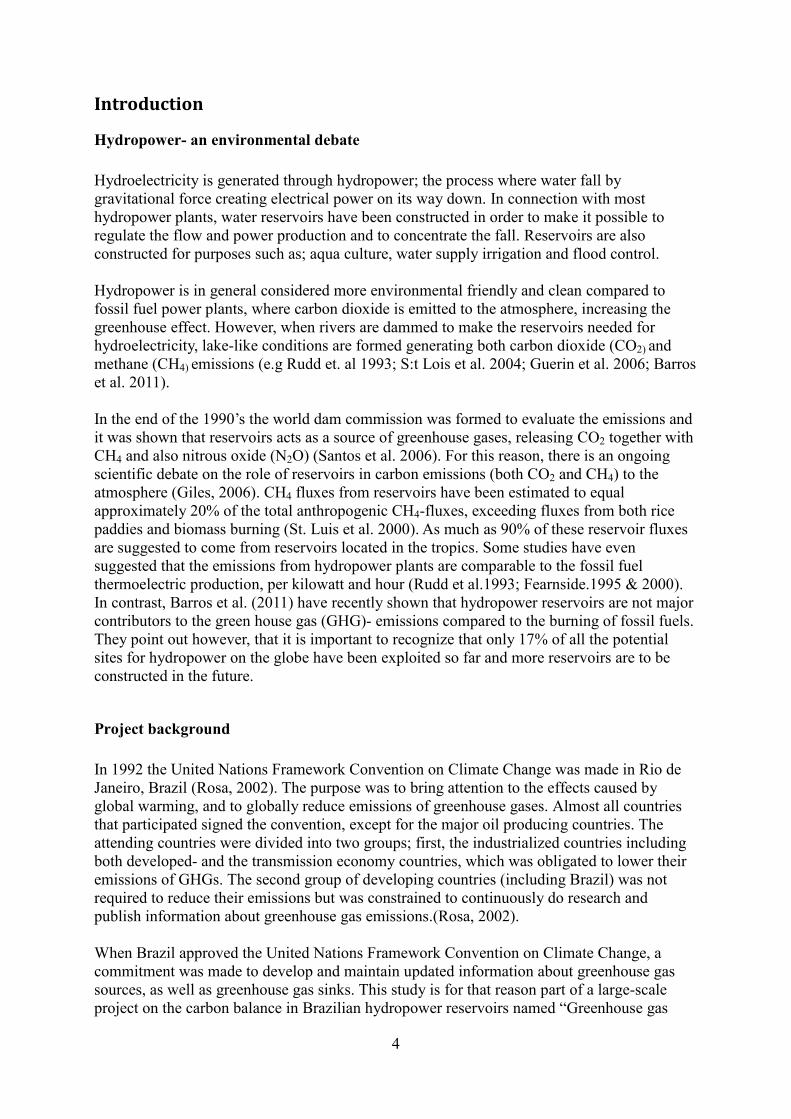
Hydropower- an environmental debate Hydroelectricity is generated through hydropower; the process where water fall by gravitational force creating electrical power on its way down. In connection with most hydropower plants, water reservoirs have been constructed in order to make it possible to regulate the flow and power production and to concentrate the fall. Reservoirs are also constructed for purposes such as; aqua culture, water supply irrigation and flood control. Hydropower is in general considered more environmental friendly and clean compared to fossil fuel power plants, where carbon dioxide is emitted to the atmosphere, increasing the greenhouse effect. However, when rivers are dammed to make the reservoirs needed for hydroelectricity, lake-like conditions are formed generating both carbon dioxide (CO2) and methane (CH4) emissions (e.g Rudd et. al 1993; S:t Lois et al. 2004; Guerin et al. 2006; Barros et al. 2011). In the end of the 1990’s the world dam commission was formed to evaluate the emissions and it was shown that reservoirs acts as a source of greenhouse gases, releasing CO2 together with CH4 and also nitrous oxide (N2O) (Santos et al. 2006). For this reason, there is an ongoing scientific debate on the role of reservoirs in carbon emissions (both CO2 and CH4) to the atmosphere (Giles, 2006). CH4 fluxes from reservoirs have been estimated to equal approximately 20% of the total anthropogenic CH4-fluxes, exceeding fluxes from both rice paddies and biomass burning (St. Luis et al. 2000). As much as 90% of these reservoir fluxes are suggested to come from reservoirs located in the tropics. Some studies have even suggested that the emissions from hydropower plants are comparable to the fossil fuel thermoelectric production, per kilowatt and hour (Rudd et al.1993; Fearnside.1995 & 2000). In contrast, Barros et al. (2011) have recently shown that hydropower reservoirs are not major contributors to the green house gas (GHG)- emissions compared to the burning of fossil fuels. They point out however, that it is important to recognize that only 17% of all the potential sites for hydropower on the globe have been exploited so far and more reservoirs are to be constructed in the future.
Project background In 1992 the United Nations Framework Convention on Climate Change was made in Rio de Janeiro, Brazil (Rosa, 2002). The purpose was to bring attention to the effects caused by global warming, and to globally reduce emissions of greenhouse gases. Almost all countries that participated signed the convention, except for the major oil producing countries. The attending countries were divided into two groups; first, the industrialized countries including both developed- and the transmission economy countries, which was obligated to lower their emissions of GHGs. The second group of developing countries (including Brazil) was not required to reduce their emissions but was constrained to continuously do research and publish information about greenhouse gas emissions.(Rosa, 2002). When Brazil approved the United Nations Framework Convention on Climate Change, a commitment was made to develop and maintain updated information about greenhouse gas sources, as well as greenhouse gas sinks. This study is for that reason part of a large-scale project on the carbon balance in Brazilian hydropower reservoirs named “Greenhouse gas

5
emissions from hydroelectric reservoirs in Brazil” sponsored by the Brazilian National Hydropower Energy (Eletrobrás). The intention is to investigate the extent of hydropower reservoirs and the effects of building new reservoirs in relation to greenhouse gas emissions (Brazilian Project, 2012). The main goals of “Greenhouse gas emissions from hydroelectric reservoirs in Brazil” are:
“To determine emissions of carbon dioxide (CO2), methane (CH4) and nitrous oxide (N2O) from hydro electric reservoirs in Brazil.
To identify the pathways of the carbon cycle in these reservoirs, as well as the environmental factors involved in it.
To evaluate the influence of morphological, morphometric, biogeochemical and operational variables on the greenhouse gas emissions.
To establish the previous pattern of greenhouse gas emission, prior to the flooding of the reservoirs.
To develop a spatial and temporal model of the greenhouse gas emissions in reservoirs that flood Cerrado environments in Brazil.” (Brazilian Project, 2012.)
The present study was also sponsored by SIDA (Swedish International Development cooperation Agency) through a minor field study (MFS). MFS is a scholarship program for students and teachers for field studies in developing countries. The intention of the program is to spread knowledge in different sciences and to enhance international relationships around the world.
Main objectives It is important to improve available information and to develop tools to investigate the greenhouse gas status in reservoirs in order to make decisions and reduce emissions from hydro power. Although research suggests that emissions in cold and temperate climates are generally low compared to fluxes from tropical climates (eg. S.t Loius et al. 2000; Tremblay et al. 2005; Marotta et al. 2009; Roland et al.2010) a major part of the studies made so far have been completed in the northern hemisphere and tropical regions are highly underrepresented. In the broadest analysis of greenhouse gas emissions from ~5000 lakes (Sobek et al. 2005), only ~2% represented tropical lakes. In addition, most of the studies in this area have been connected to CO2 emissions, neglecting the even stronger greenhouse gas of CH4. More research is therefore needed to explore the characteristics of the CH4 emissions in the tropics. The purpose of this study was to estimate tropical CH4-fluxes in three different hydro power reservoirs in Brazil with different characteristics. The main question was: What is the impact of carbon-, nutrient- and oxygen levels on CH4-fluxes within and between the tropical reservoirs? To answer this question the CH4-emission rates were compared between different carbon-, nutrient- and oxygen status among and between three reservoirs in Brazil. In addition a minor emergent plant experiment was conducted to see whether macrophytes have a central role in the transmission of CH4 to the air.

6
Other control variables such as: conductivity, depth, pH, secchi depth, temperature , turbidity, and wind speed that also can be linked to CH4- fluxes or help to characterize the reservoirs was also measured.
Hydropower- in Brazil and globally In Brazil as much as ~90% of all energy derives from hydroelectricity (NSF, 2011). There are 2200 hydropower plants within the country (NSF, 2011) of which 400 are considered large- and medium-sized (Rosa et al. 2004). Even so, the country imports energy from surrounding countries. To be able to feed the growing need of energy the Brazilian government plan to extend the use of this energy source even more by building 494 new dams until the year 2015. Since year 2000, 50 new hydropower plants have already been built and another 70 hydropower plants are planned to be build (NSF, 2011). It has been estimated that ~30% of the total potential of hydropower capacity is in use in Brazil today (comparable to 97% in France, 70% in Germany, 68% in USA) (Swedish embassy, Brasilia), but the regions with hydropower and reservoirs are geographically unevenly distributed. In the southern, south- and north-eastern regions hydropower has nearly reached its full capacity (Figure 1) leaving the remaining 70%-part of potential hydro power capacity located in the ecologically fragile Amazonian region. This leads to major problems. First, energy produced in the northern region has to be transported long distances to the southern parts of Brazil where the energy consumption is larger due to a higher population density, and higher industry production. A loss of ~15% in distribution and production, due to long transports along electrical networks, has been estimated to occur (Swedish embassy, Brasilia). Secondly, environmental negative effects are seen when building the reservoirs where the local environmental effects are direct and extensive. Also, social problems are created when large construction projects forces thousands of people to relocate, most of them indigenous people, changing their culture and way of living. Globally, the total surface area of reservoirs most cited is around 400 000km2 (Cole et al.2007), but this area is constantly increasing as the demand for hydroelectric power, agriculture and domestic use is growing. According to a more recent estimate the area of all types of reservoirs in the world is approximately 500 000km2 (Lehner et al. 2011). Large impoundments around the world are thought to increase with 1-2% every year (Downing et al. 2006), which means that in 2050 the area of dammed regions will be close to 1 000 000 km2 (Tranvik et al. 2009). Today, water is already being retained by dams corresponding to a reduction in the global sea level rise by 0.55 mm/year over the past 50 years (Chao et al. 2008).
The role of freshwater systems to greenhouse gas emission Previously, freshwater systems have been neglected as a potentially important part of the carbon cycle. Simplified, the carbon cycle has been considered to consist of two biologically
Figure 1. The red circle display the region where hydropower has nearly reached it fully capacity in Brazil, leaving the remaining 70%-part of potential hydropower capacity in the ecologically fragile Amazonian region (green circle).

7
compartments; land and oceans, connected to a third component (air) through gas exchange. It has later on been shown that rivers transports significant amounts of terrestrial carbon (both inorganic and organic) to the oceans (e.g. Schlesinger and Melack 1981), working as a “transportation bridge” of carbon between land and sea. Cole et al. (2007) showed that the transfer of terrestrial carbon to freshwater system is actually larger than the amount delivered to the sea. Estimations showed that inland waters annually receive ~1.9 Pg C/year from the terrestrial landscape (both from background and anthropogenically altered sources), of which about 0.2 is buried in aquatic sediments, 0.9 Pg C/year is delivered to the oceans and at least 0.8 Pg C/year is returned to the atmosphere as gas exchange. This shows that the role of freshwater systems in relation to the natural carbon cycle is fundamental and of great importance when it comes to GHG-emission to the atmosphere. Since most of the lakes in the world are supersaturated with CO2 , they will also emit CO2 to the atmosphere (Cole et al. 1994 ; Sobek et al. 2005; Roland et al. 2010). Increasing the surface area of freshwater systems (as when damming up water) will thus consequently increase the carbon-flux to the atmosphere. When rivers are dammed to make the reservoirs needed for hydroelectricity, lake-like conditions are formed generating CO2 and CH4. The flooding also releases carbon bound to surrounding soils and destroys all terrestrial plants in its way. The latter results in the loss of a very important sink for atmospheric CO2 since plants assimilate CO2 by photosynthesis, and thus affecting the net CO2-level in the atmosphere. In addition, all the organic matter from the terrestrial plants is decomposed by bacteria and greenhouse gases are thereby released to the atmosphere (St Lois et al. 2000).
CO2- and CH4- production within reservoirs CO2 and CH4 are two of the main greenhouse gases created by anthropogenic activities. CO2 is produced during the combustion of nearly any organic material whereas CH4 has a variety of industrial sources. These two greenhouse gases are also both produced naturally and the reactions occur particularly in wetlands and lakes and are formed during microbial decomposition of organic matter. The source of organic matter, particulate and dissolved carbon (POC, DOC) is obtained from surrounding catchment areas and from biomass within the water system such as litters, soils, trunks and leafs falling into the water.
CH4 is produced by decomposition under anoxic conditions in the deeper layers of the water column or in the sediments by methanogenic microorganisms (methanogens) (Bastviken, 2009). The two major anaerobic microbial pathways are 1) acetate dependent methanogenesis, where acetate (CH2COO) is cleaved into CH4 and CO2 and 2) hydrogen dependent methanogenesis, where H2 reacts with CO2 forming CH4 and water. Methanogenesis is the final step in the decay of organic matter under anaerobic conditions. It was previously thought that methanogenic bacteria only exists in strictly anaerobic environments but it is now established that any methanogens can stand some levels of oxygen. Yet no methanogenesis occurs in oxic conditions. (Bastviken, 2009).
In the upper oxic layer of the water column CO2 is produced by aerobic decomposition of POC and DOC (Rosa et al. 2002). In presence of CH4 and oxygen, metanotrophic bacteria can use the energy of CH4 and oxidize it into CO2. This process can occur when the CH4 produced in the sediments diffuses upward into more oxygenated water. The CH4 is when oxidized transformed sequentially into methanol, formaldehyde, formate and finally to CO2 (Bastviken, 2009).

8
The new lake-like environment, with a deeper static system instead of a more turbulent and shallow one, created when damming up promotes a shift from CO2 emission to the even stronger greenhouse gas CH4 (Rosa et al. 2002). These conditions (slower retention time and lesser turbulence) make the water more anoxic, which is favorable of CH4-production. The mass of methane emission is a minor fraction of the total carbon mass transfer and is shorter lived in the atmosphere compared to CO2 but is still very important since the global warming potential of CH4 is 25 times greater relative to CO2, over a 100-year period (IPCC, 2007).
Flux pathways of CO2 and CH4 in reservoirs The greenhouse gases can be released in several ways within the reservoir or in connection to the hydroelectric power plant. CH4 emits to the atmosphere by either diffusion or ebullition and can also be oxidized into CO2 and transported to the surface as already mentioned. Figure 2 shows four pathways within a reservoir where GHGs are released to the atmosphere.
1. Diffusion. Gas exchange between the surface water and the atmosphere occurs by diffusion and is driven by concentration differences between the media. Since CH4 solubility is very low in water, surface waters are almost always oversaturated with 3-3000 times more CH4 in water than in air (Bastviken, 2009). Very low diffusion rates can also occur between the sediment-water phase and the water- air phase, similar to molecular diffusion. In both cases, the diffusive flux is slow and hence enables oxidation in oxic layers. The transport of CH4 from the sediment to the water column is mainly due to turbulence-induced diffusion (also called eddy diffusion) and the diffusive flux is enhanced by high water surface concentrations and turbulence in the surface water, which increases the water surface in connection to the air (Bastviken, 2009). Gas fluxes by diffusion are much greater than by bubbling for CO2 and ~99% of the CO2 emissions come from diffusive flow (Rosa et al. 2000). For methane, diffusion into the atmosphere is more difficult to estimate and has been measured in a range of 14-90% of total flow. CH4 -flux intensity in reservoirs varies with time, but the fluctuations appear to be
Figure 2. Four different pathways where greenhouse gases are released in a hydropower reservoir: 1) Diffusion: Gas exchange through the air-water interface driven by concentration differences. 2) Ebullition: Bubble formation in the sediments due to hydrostatic pressure and turbulence. 3) Downstream emission: Turbulent water mixes the sediment and the water column which increases emissions. 4) Plant-mediated flux: emissions through the stems of macrophytes.

9
driven by a strong random component (Rosa et al. 2002) and emissions are therefore hard to modulate. 2. Ebullition. Ebullition of CH4-bubbles occurs when gas escape from the sediments and rapidly pass through the water column, without the chance of getting oxidised into CO2. Ebullition accounts for ~50 % or more of the CH4-release from open waters (Bastviken, 2009), but is, as already mentioned, hard to estimate and range between 10-86 % according to Rosa et al. (2002).The bubble formation is dependent on hydrostatic pressure and depth is therefore an important parameter, where shallow sediments with low hydrostatic pressure are found to release more ebullition bubbles (Bastviken, 2009). Higher rates of ebullition have also been observed when the air pressure is low, usually followed by cold fronts and stormy weather. Rain and winds increases the turbulence among the sediments, which can increase the ebullition- and diffusion rates. Ebullition follows an episodic pattern and is not homogeneous spatially distributed which makes it even more difficult to estimate the emissions. 3. Downstream emissions. Higher emissions of GHG.s downstream a dam has been shown (Abril, 2005; Guerin el al. 2006; Kemenes et al 2007). Water that passes through the turbines in a hydro plant is often taken from deep and CH4-rich water from the reservoir. When this water is exposed to the atmosphere the hydrostatic pressure instantly drops and the gas is rapidly released (Kemenes et al. 2007). The massive water volumes that are released downstream a dam also causes a turbulent mixture of the water column with the sediments which increases the emissions of CH4. 4. Emergent plant-mediated emissions. Many aquatic plants have developed an internal gas-space ventilation system in order to facilitate oxygen transport from shoots to roots. Within the same system gases (e.g CH4) from the sediments can be taken up by the roots and be transported to the atmosphere via leaves and old shoots. Thus, emergent plants can function as conduits for CH4 to reach the atmosphere. These systems can either be pressurized or passive depending on the plant species (Brix et al 1992; Joabson et al. 1999; Bastviken, 2009). The ability to pressurize varies with temperature and water-vapor pressure (Brix et al. 1992). Plant-mediated emission dominates from most lakes and wetlands and it has been observed that fewer ebullition bubbles occur where there are rooted plants growing (Bastviken, 2009).
Important factors affecting the fluxes Emissions of CH4-(and CO2) from hydroelectric reservoirs depend on several interacting factors. It is therefore difficult to recognize and predict the variables most important regarding CH4-fluxes. Different factors are discussed below, starting with carbon-, nutrient- and oxygen levels that are in main focus. Organic matter: There are differences in the total input of particulate organic carbon (POC), dissolved organic carbon (DOC) and inorganic carbon (DIC) in global rivers and lakes (Meybeck, 1993). The different carbon inputs and emissions from lakes and reservoirs reflect difference in; climate, surrounding soil textures, fauna and flora, land use and also geochemistry (Meybeck, 1993). In boreal forests with carbonate rich terrain, and in temperate regions, DIC is the dominant input to freshwater systems, due to carbonate weathering, high soil respiration and groundwater flow, whereas DOC dominates in tropical regions and in

10
non-carbonate boreal forests (Tranvik et al. 2009). In higher northern Arctic latitudes DIC may also be of major input. The movement of POC and DOC in freshwater systems is different from one another (Battin et al. 2008). DOC moves with the water, whereas POC is heavier and tends to sink to the bottom and is also subject to hydrodynamic lift and drag forces. To be able to use POC as energy, microbial extracellular enzymes have to first hydrolyze POC into smaller elements. The resulting DOC-molecules can then be used in microbial metabolism. Hence, DOC is the most important intermediate of carbon cycling since only low molecular weight compounds can be transported through the microbial cell membrane and subsequently be metabolized (Battin et al. 2008). Nutrients: Emissions are thought to increase with nutrient levels since nitrogen and phosphorus are essential for primary production. In eutrophic reservoirs a larger amount of decomposed organic matter fixed by photosynthesis is recycled as CO2 in oxic waters and CH4 in anoxic conditions. High primary production during the summer may reduce emissions to the atmosphere through algal fixation of CO2, making eutropic lakes under saturated and work as a sink of CO2. However, most of this carbon will in the end be composed and returned to the atmosphere (S:t Louis et al. 2000). Some of the highest CH4 fluxes have been recorded in the most eutrophic systems (Barros et al. 2011). Oxygen: Anoxic conditions are crucial for methanogenesis to occur as already mentioned. In presence of CH4 and oxygen, metanotrophic bacteria can use the energy of CH4 and oxidize it into CO2. Therefore, oxygen levels in a reservoir decide whether CH4 or CO2 is to be produced and emitted when the organic matter is decomposed (Rosa, 2004; Bastviken, 2009). Age: The age of the reservoir affects the greenhouse gas fluxes with higher emission from younger reservoirs compared to old ones. This is because newly flooded organic matter, such as leaves and litter is thought to decompose faster than decomposition of older and more robust carbon such as peat and soil carbon (Kelly et al.1997; S:t Luis et al. 2000). pH and salinity: pH does not seem to limit methanogenesis but can indirectly affect the substrates available for usage of bacteria (Bastviken, 2009). Acetate dependent methanogenesis seems to be favored at low pH, whereas H2-dependent methanogenesis is favored at higher pH. Both types can occur simultaneously with either process contributing between 20-80% of the overall CH4 production. There is no clear pattern on how pH affects CH4-oxidation rates, but bacterial communities are probably adapted to different pH-values (Bastviken, 2009). pH also regulates the form of DIC. In rivers DIC exists mostly in the form of HCO3- where the pH range usually is between 6- 8.4 (Meybeck, 1993). Lower pH is favorable for CO2 since high pH lower CO2 concentrations relative to bicarbonate (HCO3
-) and CO3
2- which is retained in the water. Since saline and hard water lakes contribute to almost half of the global volume of inland water (Wetzel, 2001), they are very important in the global carbon budget, although high salinity inhibits CH4 oxidation (Bastviken, 2009) Temperature: Higher temperature increases all biological processes, including the decomposition of organic matter by bacteria which enables CH4 and CO2 release to the atmosphere. CH4 oxidation rates seem less sensitive to temperature compared to methanogenesis (Bastviken, 2009). Both respiration and primary production is amplified with a higher temperature. However, it has been argued (e.g. Lopez-Urrutia et al. 2006; Sand-Jensen et al.2007), that respiration usually has a stronger response, leading to a net increase of

11
CO2 emissions when it is warmer (Kosten et al 2010). The amount of gas being released across the water-air phase depends on the gas solubility in water. The gas solubility is positively correlated to pressure and negatively correlated to temperature (Le Chatalier’s principle). Hence, CH4- and CO2-emissions through diffusive flux is likely to be higher in reservoirs located at lower altitude and warmer regions (Mendonça et al. 2012). Temperature is a central factor linked to many parameters in the next sections. Stratification: Just like lakes, reservoirs tend to undergo thermal stratification which prevents the water to mix. Thermal stratification is triggered by density differences of water carrying different temperatures and leads to the formation of different water layers: epilimnion (top), metalimnion (intermediate) and hypolimnion (bottom). Large amounts of CH4 can therefore be trapped in the anoxic hypolimnion. When mixture of the water column does occur, massive amounts of greenhouse gases are rapidly released to the atmosphere. Due to persistent stratification of reservoirs located in warmer regions, methanogenesis is more common (Bastviken, 2009; Mendonça et al.2012). Latitude: Emissions from reservoirs have been shown to be higher in tropical regions (S.t Loius et al. 2000; Tremblay et al. 2005; Marotta et al. 2009; Roland et al.2010) and have a higher emission rate of gases compared to temperate regions. The higher temperature and the latitudinal differences of the total input of POC, DOC and DIC, already mentioned, in tropical regions affects the total sum of the total emission. In addition, the sediments and the bottom layers often are anoxic in tropical regions, contributing to a shift towards CH4 emissions (Barros et al. 2011). Weather: Flux-measurements of CH4 can vary with high frequency and are greatly dependent on external factors such as weather conditions. Wind and rain mixes the water and produces turbulence which can increase the emission of green house gases (Unesco, 2009).
Material and Methods
Summary of procedure To investigate CH4-emissions at the air-water interface in the reservoirs, floating static chambers were used. The principle is to trap the gas that is released from the water surface. From this it is possible to calculate the emission flow rate by calculating the linear rate of gas accumulation in the chambers over time. In every reservoir a number of stations were selected to represent the reservoir and to be able to see the spatial distribution. Three floating static chambers (replicates), connected to a boat, were put into the water at every station and an initial sample of air and water was taken. Gas was collected from the chambers with a syringe every 10 minutes for a period of 30 minutes and put into vials. To make sure that no air could contaminate the samples, the vials were filled with saturated water that was emptied simultaneously as the vials were filled with sample gas. The gas inside the vials was then analyzed with a gas chromatograph (GC) and the concentration of methane obtained could then be used to calculate the flux. At all stations the other variables (such as conductivity, depth, pH, secchi depth, temperature, turbidity, and wind speed) was also measured.

12
Preparation
Building the chambers Three chambers made of plastic containers were built and used as three replicates (Figure 3). The surface areas of the headspace were ~1665 cm2 and the volumes were 35.75 l. Metallic reflecting material was glued onto the outside of the open-bottom chambers to reflect sunlight. A rope was attached around the chambers using aluminum tape and to this rope floating buoyant could be tied on to by cable ties. The buoyant was attached approximately 10 cm from the bottom edge of the chambers so that 10 cm of the chamber would be underneath the water surface. This was to make the chamber more stable in turbulent waters, preventing air to leak in from the sides. A small hole was made (ø=1.2 cm) in the roof of each camber where a rubber-stopper could fit. An even smaller hole was made through the rubber-stoppers (ø=0.5 cm) were a 20-25 cm plastic hose connected to a three-stop (a special kind of valve) was joint. The rubber-stopper together with its plastic hose was fixed with silicon, making sure no external air could contaminate the samples.
Preparing the vials
All vials were pre-filled with water to make sure the samples were not contaminated with air. The water was saturated (~320g salt/l) in order to prevent gas exchange to take place between our gas samples and the water, which could have change the actual concentration maintained. A large set of salt solution was made were the vials could be dipped in. Each vial was completely filled and sealed with a rubber-stopper. To prevent air bubbles to occur a needle was put through the rubber-stopper which were directly put on to the vial so that surplus water from the vial could escape through the needle, leaving no space for air. The needle was then carefully removed so that the rubber-stopper enclosed the needle-hole, “unmaking” it. The closed vials were then sealed with a metal-lid. It is important that no air bubbles exists when sealing the vials with rubber-stoppers and metal-lids. However, it should be noticed that a temperature change could create “bubbles” in the vials, but in this case “vacuum-bubbles” since the volume of the salt solution decreases with decreasing temperature and vice-versa.
Figure 3a and b. Chambers used for measurements of CH4 emissions from reservoirs.
a b
13
Sampling procedure
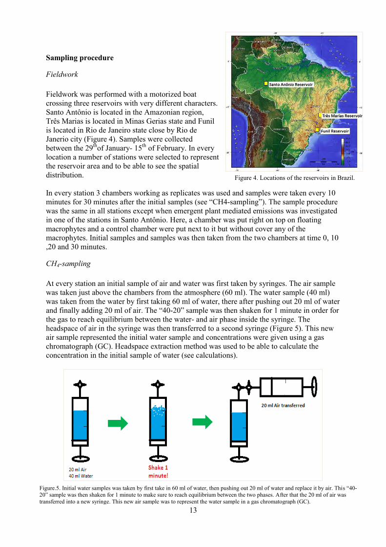
Fieldwork Fieldwork was performed with a motorized boat crossing three reservoirs with very different characters. Santo Antônio is located in the Amazonian region, Três Marias is located in Minas Gerias state and Funil is located in Rio de Janeiro state close by Rio de Janerio city (Figure 4). Samples were collected between the 29thof January- 15th of February. In every location a number of stations were selected to represent the reservoir area and to be able to see the spatial distribution. In every station 3 chambers working as replicates was used and samples were taken every 10 minutes for 30 minutes after the initial samples (see “CH4-sampling”). The sample procedure was the same in all stations except when emergent plant mediated emissions was investigated in one of the stations in Santo Antônio. Here, a chamber was put right on top on floating macrophytes and a control chamber were put next to it but without cover any of the macrophytes. Initial samples and samples was then taken from the two chambers at time 0, 10 ,20 and 30 minutes.
CH4-sampling At every station an initial sample of air and water was first taken by syringes. The air sample was taken just above the chambers from the atmosphere (60 ml). The water sample (40 ml) was taken from the water by first taking 60 ml of water, there after pushing out 20 ml of water and finally adding 20 ml of air. The “40-20” sample was then shaken for 1 minute in order for the gas to reach equilibrium between the water- and air phase inside the syringe. The headspace of air in the syringe was then transferred to a second syringe (Figure 5). This new air sample represented the initial water sample and concentrations were given using a gas chromatograph (GC). Headspace extraction method was used to be able to calculate the concentration in the initial sample of water (see calculations).
Figure.5. Initial water samples was taken by first take in 60 ml of water, then pushing out 20 ml of water and replace it by air. This “40-20” sample was then shaken for 1 minute to make sure to reach equilibrium between the two phases. After that the 20 ml of air was transferred into a new syringe. This new air sample was to represent the water sample in a gas chromatograph (GC).
Figure 4. Locations of the reservoirs in Brazil.

14
After the initial samples, samples were taken with syringes from the chambers in every 10 minutes for 30 minutes (3 times). All samples (initials- and 10-20-30-minutes samples) were injected with a needle into the rubber-stoppers, maintaining the vials bottom-up while simultaneously expelling the saturated water through a second needle (Figure 6). When approximately 20-30 ml of sample air had been injected into a vial the second needle was carefully removed before all the saturated water was expelled through it. This was in order to keep an overpressure and water in the vial so that no external air could leak in.
Other sampling All other sampling was collected by members from the Federal University of Juiz de Fora. Dissolved and saturated oxygen, carbon- and nutrient levels, partial pressure of CO2 (pCO2), temperature, pH, wind speed, depth and secchi depth was measured and analyzed. Carbon: Water samples for measurements of total organic carbon (TOC, DOC and DIC) were analysed using a Carbon Analyzer (Phoenix 8000), where the total dissolved organic carbon was measured as CO2, following high temperature oxidation with a UV lamp. Before TOC analysis, inorganic carbon was eliminated from the samples by phosphoric acid addition and sparging for 6 min with N2 – free air. At least three measurements of TOC were made for each sample; the coefficient of variation (CV) was considered acceptable when less than 2%. Nutrients and Chlorophyll-a: For analysis of chlorophyll a (Chl a) concentrations, integrated epilimnion water was filtrated onto a GF/F filter that was stored frozen before analysis. For analysis of phosphorus, nitrogen and chlorophyll, water was collected using a Jorg bottle (Hidrocean), at the surface and at the depths of 10 and 1% light penetration (determined from the Secchi transparency, as recommended by Esteves, 1988). CO2, Conductivity, pH and Temperature: Concomitant with the CO2 work, samples for other water chemistry measures (alkalinity, temperature and, pH) were taken using a polyethylene bottle. Water used for pCO2 measurements was taken at 0.5-m depth between 8:00 and 12:00
Figure 6. The samples taken at 10,20 and 30 minutes after the initial samples was injected to vials filled with saturated water. First a needle was put halfway through the rubberstopper maintaining the vial bottom-up. A second needle connected to the syringe with gas sample was then pressed through the rubberstopper and when the first needel was pressed all the way through, water was released simultaneously as air filled the vial.

15
a.m. Measurements of pCO2 was made directly using the membrane equilibrium method (Hesslein et al. 1991; Cole et al. 1994). Gas was immediately measured using an infrared gas analyzer (IRGA – environmental gas monitor EGM-4; PP Systems). Additional data for pH, surface temperature and conductivity were obtained by attaching a sonde (YSI model 6920), and exchanging and calibrating it every 15 days according YSI Environmental Operations Manual (www.ysi.com/ysi/support). Standard solutions (pH 4, 7, and 10) were used to calibrate each pH sensor. Alkalinity (ANC) was also measured by titration using 0.01N sulfuric acid. Wind speed: was measured in every station with a portable anemometer. Secchi depth: Water transparency was measured by Secchi disk.
GC-measurements A gas chromatograph (GC) (at the Department of Ecology, University Federal of Rio de Janeiro, Brazil) equipped with a flame ionization detector (FID) was used to analyze the CH4 and some CO2-samples. The GC is very sensitive to external factors such as temperature. Because of time constraint, initial samples and samples taken after 30 minutes were prioritized and often analyzed first in the GC, while samples from 10 and 20 minutes were analyzed later on. Since all initial water samples exceeded the initial air concentrations a positive flux was expected. Concentrations obtained in 10 and 20 minutes were however lower than the initial air values in some cases. This is probably because they were analyzed in a different time and the temperature, in the room where the GC was situated, had changed. It was therefore decided only to use the concentrations obtained after 30 minutes from the three replicates when later on calculate the flux (Figure 7), instead of measuring the flux in the different times (0,10, 20 and 30 minutes) to see how the flux-rate changed over time, which was the original idea.
Figure 7. Since all initial water samples exceeded the initial air concentrations a positive flux was expected.
Concentrations obtained in 10 and 20 minutes was however lower than the initial value in air in many cases. It was therefore decided to use the concentrations obtained at 30 minutes.
0
0.5
1
1.5
2
2.5
0 10 20 30
[CH4] (ppm)
Time (min)
Funil 2
yellow chamber
red chamber
blue chamber
Average
Values which fluxes are based up on

16
Study Areas
Funil In Funil fieldwork was performed between the 29-30th of January and 12 stations were selected all through the reservoir (Figuree 8). Five stations were sampled in the first day (1-5) and high precipitation levels were observed (data not shown). Six stations (6-12) were sampled in the second day with better weather conditions. The median water depth was low (~5m below highest level) and the water had a very green color due to cyano bacteria presence, shown by previous studies (Soares et al. 2008).
Table.1. Characteristics of Funil reservoir The Funil reservoir was constructed in 1969 by the damming of the river Paraiba do sul. The reservoir is located at a very industrial area outside Rio de Janeiro and Paraiba do Sul River belongs to the Coastal Southeast hydrographical region. It drains and receives waste from the most populated area in the country, crossing lands of both Sao Paulo and Rio de Janeiro state and draining out to the Atlantic sea (see Table 1 for reservoir characters). Climate conditions are characterized by wet summers and dry winters. The vegetation around the reservoir is very poor, due to previous coffee plantations. The constant water level fluctuation causes erosion along the bank which settles in the reservoir (Branco et al. 2002).
References: Coordinates: 22 35’S - 44 35’W Roland et al. (2011) Area: 40 km2 Branco et al. 2002 Altidtude: 440 m Branco et al. 2002 Volume: 890 106 m3 Branco et al. 2002 Max Depht: 70 m Branco et al. 2002 Mean Depth: 22 m Branco et al. 2002 Residence time: 10- 50 days Soares et al. (2008) Outlet position: Epilimnion Roland et al. (2011) Annual Mean Air Temp:
18.4 C Roland et al. (2011)
Annual precipitation:
1.337mm Roland et al. (2011)
Figure 8. A map of Funil reservoir with 12 sampling stations

17
Limnological studies have been performed in the reservoir for over a year (Soares et al.2008). Due to a short retention time (10-50 days) a dynamic system with a pronounced temporal pattern was seen. This temporal pattern is thought to be related to changes in the water column and phytoplankton biomass. The reservoir is thermally stratified during the summer (December-February) with isothermy and four mixing periods: 1) June-Oct 2) Nov- Dec 3) Jan- Mar 4) April-June. The highest precipitation and temperature levels were seen from November to Mars (Soares et al.2008). The system was very turbid with a low euphotic zone, especially in period 2 which corresponds to a higher biomass of phytoplankton with a peak in December. The pH was alkaline at the surface, especially during period 1 and 3 but in the end of period 3 and in the beginning of period 4 the whole water column was acidic, reaching higher values again in period 2 (pH: 8.7). In the 1970s Funil was considered to be mesotrophic but has over the years experienced massive eutrophication with repeatedly intense cyano bacterial blooms, and nutrient levels was shown to be high all through the year. Dissolved oxygen measurements also made showed a slightly chemical stratification only during period 1 with decreasing oxygen levels from surface to bottom. However, anoxic conditions could not be seen (Soares et al.2008), which is not expected from a highly eutrophic water system.
Santo Antônio reservoir The field work in Santo Antônio was completed between the 4-8th of February and 10 stations were selected (Figure 9). Three of them (station 8, 9 and 10) were located downstream the dam and due to a lot of turbulence here and because a restricted amount of vials, full observations could not be done. Thus, only initial water- and air-samples was taken in these three stations. Emergent plant-mediated emissions were investigated at station 7. The water level was overall high (3m below highest point) but would become even higher and reach the highest level in March. The water level usually differs 15 m between summer and winter with more precipitation during the winter. Erosion processes were observed where a lot of mud and vegetation was released from the terrestrial landscape. The color of the water was brown/red most of the time due to suspended organic material. In some places the water was really dark and looked black. Santo Antônio reservoir is located in the Amazonia-region and has a size of 271 km2. Its main tributary is Madeira River which derives from the Andes in the west. Madeira river is the largest, out of four (McClain and Naiman,2008) tributaries of the Amazon river, contributing with around 16% of the Amazon discharge (Moratti and Probst, 2003). The Madeira basin has a humid tropical climate (according to Köppens classification) with an annual mean precipitation of 1900-2200mm Temperatures are ~40 C in the dry season and ~25-30 C in the wet season (personal communication Rafael Almeida). The dry season is in May-September and the wet season in October-April. Annual average discharge has been calculated to 19 x 103 m3/s (Leite et al.2011). The river passes the city Porto Velho, with approximately 426 000 residents, along its course. The drainage area of Porto Velho corresponds to 69% of the total basin area of Madeira river (Leite et al. 2011). The plan is to extend the hydropower in this area by constructing four hydroelectrical complexes, two of them located in near Porto Velho; Santo Antônio and Jirau. Together these two power plants will be the third largest hydro power complex, generating

18
6450 mega watt of electricity (Leite et al. 2011), where most of it will be transported to southern-eastern regions.
Figure 9. Santo Antônio reservoir with 10 sampling stations. Station 8-10 is located downstream the dam and
only initial samples were taken here an no flux was calculated. Amazonian rivers and tributaries are classified into white-, black- and clear water which depend on their origin and nature of drainage basin (see table 2). Table 2. Ecological attributes of Amazonian whitewater, blackwater, and clearwater rivers from Junk (2011), based on the classification of Sioli (1956), Ecological attributes White water Black water Clear water pH near neutral acidic, <5 variable, 5–8 Conductivity (μS cm-1) 40–100 <20 5–40 Secchi depth (cm) 20–60 60–120 >150 Water color turbid brownish greenish Humic substances low high low Inorganic suspensoids high low low Fertility of substrate and water High low low to intermediate White water is linked to sediment load of erosion from Andean headwaters, black water emerge from decaying organic matter from low land sources and sandy soils, and clear water originates from Brazilian mountains (McClain and Naiman, 2008). White water (such as in Madeira river) transport large amounts of nutrient-rich sediments from the Andes, have a neutral pH and a relatively high concentration of dissolved solids (primarily carbonates and alkali-metals) (Junk, 2011) Black waters have a low quantity of suspended matter but have a high amount of humic acids which gives the transparent water a brownish black color. The pH is usually acidic. The fertility is low, floodplains are covered by slowly growing forest and terrestrial and aquatic herbaceous plants are scarce. Clear Water Rivers are transparent with a greenish color. Their catchments are located in the cerrado region in central Brazil. The pH

19
varies between5-8 in large rivers. The amount of dissolved solids and sediment load is low (Junk. 2011). Concerning sediment loading, white waters have high sediment input all year, whereas clear mountain waters are generally clear during dry season and whiter during wet season and during turbulent stormy events (Townsed-Small et al. 2008) A significant amount of organic matter is derived from the Andes, of which 90% is made up of fine particulate organic carbon (FPOC- less than 63 μm in diameter) (Richey et al.1990). The suspended material in Maderia River prohibit the light to penetrate the brown water column, thus prevents phytoplankton to occur, even though the river is nutrient-rich (Personal communication Rafael Almeida). In fact, the amazon floodplain is one of the most productive ecosystems on the globe where macrophytes stand for 65% of the production and floodplain forest communities for 28% (McClain and Naiman. 2008). When subtracting estimates of respiration- and burial- loss of carbon around 90Tg of carbon is available and transported to the mainstream river (Melack and Forsberg 2001; Mayorga et al. 2005). Loads of nutrients, substrates and minerals also descend from the Andes and drainages the floodplains of Madeira River. A part of these nutrients can be traced to organisms moving between the floodplain and channel. When these organisms die the organic matter and the nutrients of their bodies will serve as substrate for the ecosystem (McClain and Naima 2008.).
Três Marias The fieldwork in Três Marias was completed between 11-14th of February and 13 stations was selected (Figure 10). The water level was high since the rainy season just was about to end. The water level variation is around 2-5 m in Três Marias (Personal communication Felipe Pacheco).
Figure 10. Três Marias reservoir with 13 sampling stations.

20
Table 3 Characters of Três Marias reservoir The construction of Três Marias reservoir began in 1957 and was fully in use in 1969. The reservoir is a clear water reservoir located in Minas Gerais state in the Cerrado region. Its main tributary is São Francisco. Reservoir characters are seen in Table 3. The Três Marias-region has a tropical climate of Savanna (classification of Köppen), characterized by rainy summers and dry winters. Annual average precipitation is 1200-1300mm (Bezerra.1987 according to Fonseca et al.2007). Over the last decades the reservoir has been subject to a disordered deforestation of native species and erosion of the soil (Fonseca et al. 2007). Stratification is principally occurring during the dry season when the wind is stronger, but can happen also in the wet season due to the rain. Usually the dam is open during the dry season when more energy generally is needed (personal communication Felippe Pacheo). Limnological studies have shown that even though the Trophic State Index indicates an oligotrophic state (based on chlorophyll-a, water transparency and phosphorus levels), the high densities of zoo plankton communities makes this reservoir mesotrophic (Brito et al.2011). In a study completed in the lake Massacará (adjoining the Paraopeba River, São Francisco River Basine) high levels of zooplankton was seen especially during high water levels, although the source of nutrients and organic matter of these lakes is unclear (Sampaio and López, 2000).
Calculations By using floating chambers the diffusive flux of CH4 from the surface of the reservoirs could be estimated by calculating the linear rate of gas accumulation in the chambers over time using gas chromatography techniques. The calculations were performed according to Bastviken et al. (2004).
Fundamentals: Ptot = total air pressure (usually around 1 atm = 1013 hPa) Px =partial pressure for gas x (atm) ppm = parts per million, usually comes from GC measurement V = volume (L) n = amount of compound (mol) R = common gas constant = 0.082056 L atm K-1 mol-1 T = temperature (K) C = concentration (mol/L = M) t = time KH = Henrys Law constant (M atm-1), varies between gases and with temperature Common gas law: PV = nRT Henrys law: C = P*KH
References: Coordinates: 18o13oS Santos et al. 2006 Area: 1, 050 km2 Fonseca et al. 2007 Volume: 15*106 m3 Fonseca et al. 2007 Mean Depth: 16.8m Fonseca et al. 2007 Annual precipitation: 1200-1300mm Bezerra.1987

21
Concentration of gas in initial water sample based on headspace extraction method Headspace extraction method was used to be able to calculate the concentration in the initial sample of water. This concentration is needed to calculate the flux with a non-linear approach.“Headspace” is the closed gas volume in the syringes. From the common gas law: n in headspace (g): (1).
where Px = Ptot*(ppm/106) (atm) Vg = headspace volume (in this case 0.020 L of air in the 40:20 ml syringe extraction) T = temperature (Kelvin) when the equilibration took place n in the air: (2).
where Px in air = Ptot*(ppmairsample/106) (atm) Vg = headspace volume (in this case 0.060 L from the initial air sample). From Henrys Law: n in water (aq): (3). Where Px = Ptot*(ppm/106) (atm) and KH is selected for the appropriate gas and temperature With equation (1) and (2) the total n in vessel can be calculated: ntot = ng + naq And together with equation (3) the original concentration in the water sample can be given:
–
The Flux calculated with a linear approach: The pressure and the amount of methane (n) will increase with time inside the chamber as more gas will continuously escape from the water. The flux can be described as: (4). F =

22
Where Achamber is the area of the bottom surface of the chamber in connection to the water and tend-tinit is the deployment time. Together with the common gas law (1), where n is exchanged we get: (5).F
)
If tend-tinit is put to 1:
Extrapolation of diffusive fluxes (Compensated for decreasing flux into chamber over time; description from Bastviken et. al. 2004) By calculating the flux using a linear approach the flux can be overestimated. This is due to the fact that gas trapped inside a chamber is to have a higher concentration then if it was released and diluted in the atmosphere. Therefore a non linear calculation is in hand. The flux across an air-water interface can be formulated as follows:
(6).
where F is the diffusive flux, kg,T the gas transfer velocity of a given gas (g) at a given temperature (T) and ΔC = Cinit – Cend, the concentration gradient between the initial concentration in the water (Cinit) and the water at equilibrium with the overlying atmosphere (Cend) (Cole and Caraco,1998).
The unknown gas transfer velocity (kg,T ) depends on physical parameters which generate turbulence in the surface water and in the water column at the time of the measurement. The physical parameters for lakes, rivers and reservoirs are: windspeed, rainfall (e.g. Guérin et al., 2007) and water current velocity (e.g. Borges et al., 2004) which all have a broad and varying intensity affecting the flux (F). All increasing turbulence parameters listed above increases kg,T and thus also increases F.
Equation (6) implies that the flux is partly driven by the concentration difference which will decrease with time in the chambers. A simple calculation of the total amount of methane that entered the chambers divided with the time of measurement will hence underestimate the instantaneous flux rate. To estimate the instantaneous flux, (kg,T ) has therefore to be solved.
According to equation (3) after deleting on both sides of the equilibrium mark we get:
(7).
This equation (7) together with equation (6) leads to: (8).
23
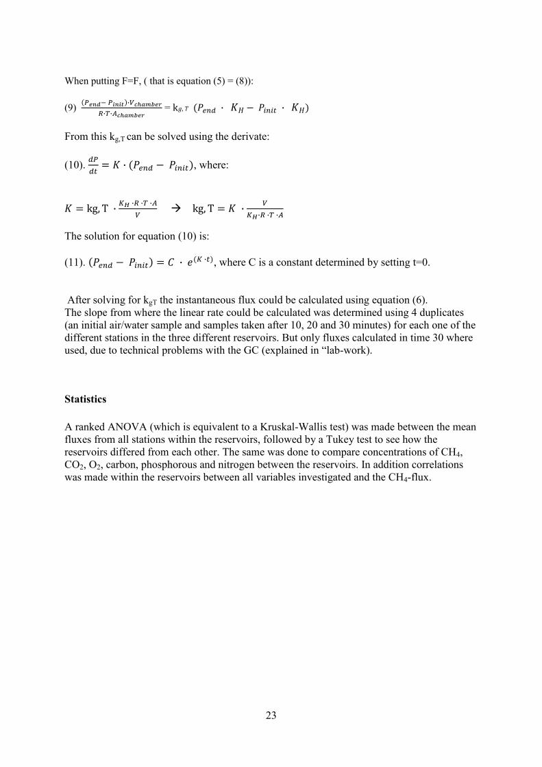
When putting F=F, ( that is equation (5) = (8)): (9)
=
From this kg,T can be solved using the derivate: (10).
, where:
The solution for equation (10) is: (11). , where C is a constant determined by setting t=0. After solving for kgT the instantaneous flux could be calculated using equation (6). The slope from where the linear rate could be calculated was determined using 4 duplicates (an initial air/water sample and samples taken after 10, 20 and 30 minutes) for each one of the different stations in the three different reservoirs. But only fluxes calculated in time 30 where used, due to technical problems with the GC (explained in “lab-work).
Statistics A ranked ANOVA (which is equivalent to a Kruskal-Wallis test) was made between the mean fluxes from all stations within the reservoirs, followed by a Tukey test to see how the reservoirs differed from each other. The same was done to compare concentrations of CH4, CO2, O2, carbon, phosphorous and nitrogen between the reservoirs. In addition correlations was made within the reservoirs between all variables investigated and the CH4-flux.

24
Results
CH4- Concentrations and Fluxes There was a wide difference between, as well as within, the reservoirs when it comes to fluxes of methane (Table 5; Figure 11). One flux-value is an average from 3 replicates taken after 30 minutes. There are 12 stations in Funil, 6 stations in Santo Antônio and 13 stations in Três Marias. Some negative values were obtained for the calculated fluxes (Santo Antônio and Três Marias), even though only fluxes based on concentrations from time 30 was included (see method). This is due to higher initial values compared to the samples taken after 30 minutes from the chamber. This is highly unlikely since the initial water samples were consistently higher than the initial air samples. The direction of the fluxes should therefore be from water to air and the flux to be positive. The negative values were however few and close to 0 and the flux can therefore be considered as none. Correlations between CH4-flux and CH4-, CO2-, oxygen-, carbon- and nutrient-levels within the reservoirs are shown in Table 4 and will be discussed more in detailed in the different result sections to come. Significant R-square values and p-values are shown in italic, bold style for CH4-concentration in Três Marias, organic carbon (both DOC and TOC) in Santo Antônio and total nitrogen in Funil. Table 4. R-square values and p-values from correlations made between variables and the CH4-flux within the reservoirs; Funil (Fu), Santo Antônio (SA) and Três Marias (TM).
Flux: CH4-conc CO2-conc O2-conc DIC DOC TOC Tot-P Tot-N Fu R2: 0.117
P:0.718 R2: -0,211 P: 0,510
R2: -0,270 P:0.396
R2: 0,255 P: 0,450
R2: 0,343 P: 0,301
R2: 0,054 P: 0,875
R2: 0,401 P: 0,222
R2: 0,765 P: 0,006
SA R2:0.634 P:0.176
R2: 0,352 P: 0,493
R2: -0,541 P: 0,268
R2: -0,364 P: 0,478
R2: 0,932 P: 0,007
R2: 0,942 P: 0,005
R2: 0,141 P: 0,789
R2: 0,335 P: 0,516
TM R2: 0.748 P:0.003
R2: 0,173 P: 0,571
R2: 0,503 P: 0,079
R2: -0,185 P: 0,544
R2: -0,287 P: 0,342
R2: 0,025 P: 0,935
R2: 0,234 P: 0,442
R2: -0,294 P: 0,329
.
Station #: 1 2 3 4 5 6 7 8 9 10 11 12 13 CH4 (ppm) Fu SA TM
21.93 3.46 1.21
4.98 34.77 2.17
2.71 1.52 6.69
13.92 15.36 2.35
3.01 6353 2.97
13.77 3.34 2.36
23.24 X
1.47
2.10 X
4.17
1.58 X
1.83
2.23 ---
1.55
2.62 ---
9.01
3.08 ---
5.64
--- ---
6.80 Flux (mmol/m2/day)
Fu SA TM
0.51 -0.27 0.00
0.31 39.60 0.00
0.28 0.42 0.00
0.65 0.07 0.11
0.03 16.13 0.20
0.39 0.41 0.02
5.75 X
-0.09
0.04 X
-0.12
9.97 X
0.08
0.17 ---
-0.01
0.21 ---
0.38
0.22 ---
0.26
--- ---
0.48
Table.5. Mean initial CH4- water concentrations and CH4-fluxes from stations located in the reservoirs Funil (Fu), Santo Antônio (SA) and Três Marias (TM). Every number is an average from the three replicates taken after 30 minutes. (X): Values are missing. (---): The station number does not exist within this reservoir.

25
-0.20
0.00
0.20
0.40
0.60
0.00
2.00
4.00
6.00
8.00
10.00
1 2 3 4 5 6 7 8 9 10 11 12 13
Flu
x (m
mo
l/m
2/d
ay)
[CH
4] (
pp
m)
Station number (1-13)
Três Marias
Conc CH4-Flux
-2.00
0.00
2.00
4.00
6.00
8.00
10.00
12.00
0.00
5.00
10.00
15.00
20.00
25.00
1 2 3 4 5 6 7 8 9 10 11 12
Flu
x (m
mo
l/m
2/d
ay)
[CH
4] (
pp
m)
Station number (1-12)
Funil
-10.00
0.00
10.00
20.00
30.00
40.00
50.00
0.00
10.00
20.00
30.00
40.00
50.00
60.00
70.00
1 2 3 4 5 6
Flu
x (m
mo
l/m
2/d
ay)
[CH
4] (
pp
m)
Station number (1-6)
Santo Antônio
Table 5 shows initial water concentrations and mean fluxes of CH4 from every station. Even though some values are negative they still follow the same trend as the concentrations of CH4 in the water of every station (Figure 11). A significant correlation between CH4-concentration and fluxes could only be seen in Três Marias (R2:0.75; p: 0.003) (Table 4). There are two stations in Funil (7 and 9, Figure 11) that stands out and had higher fluxes. High initial concentrations in the water were seen in station 1, 4 and 7. It is clear that ebullition had occurred in station 9 since the initial concentration was low. In station 7, where the initial concentration was high, the high flux can be explained by simple diffusion. Except for station 7 and 9, fluxes in Funil were ranging between 0-1 mmol/m2/day. In Santo Antônio very high initial water concentrations and fluxes were obtained in station 2 and 5 (Figure 11). These two stations are located in black water and in tributaries of Madeira River and emitted 16 and 39.6 mmol/m2/day, respectively. All other stations are located where it is white water in the main river and the fluxes ranged between 0-0.5 mmol/m2/day. Stations 7-10 were not included since 7 is the station where emergent plant emissions was studied and 8-10 are located downstream the dam were only initial values were taken and fluxes not calculated. In Três Marias the fluxes were even and ranging between 0-0.5mmol/m2/day.
Funil and Três Marias had comparable low values when weighed against Santo Antônio (see Figure 13 and 14). Santo Antônio had in contrast a very large variance and because of the scarce sample size (6 stations excluding downstream stations and the macrophytes station), it was difficult to compare it to the other two reservoirs. There is however strong evidence that concentrations and fluxes were higher in the tributaries in Santo Antônio compared to the main river of Madeira river, something that explains the wide variation found in this reservoir.
Figure 11. Initial water concentrations and fluxes of methane are shown for every station in the three reservoirs. The numbers are an average from the three replicates taken in 30 minutes.

26
Figure12. Means of initial water CH4-concentrations and fluxes from the reservoirs: Funil (n= 12), Santo Antônio (n=6) and Três Marias (n=13). The numbers have been calculated by taking an average of initial water concentrations and fluxes in all stations within a reservoir. Figure 12 shows the difference of concentrations and fluxes between the reservoirs. The flux was ~6 times higher in Santo Antônio compared to Funil and ~80 times higher than in Três Marias. A boxplot was made to easier see medians and the variation among the groups (Figure 13). The variation was large in Santo Antônio. The two stations in Funil (7 and 9) are outliers with a lot higher initial water concentrations and fluxes. Because of the ebullition in station 9 the flux could not be calculated using the “extrapolation of diffusive fluxes”. Instead the calculation was made using a linear approach for this station. A ranked ANOVA followed by a Tukey test showed Funil and Três Marias flux- medians to be significantly different from each other (p<0.05)
Figure13. Distribution of methane-concentrations and fluxes from the reservoirs: Funil: n=12, Santo Antônio: n=6, and Três Marias: n=13. The boxes show quartiles, the inner lines (within the boxes) depict the median, and the whiskers represent the variation. Outliers are seen in Funil. Medians showed to be different in Funil and in Três Marias.

27
Initial samples
The CH4-concentrations in the water and the overlaying atmosphere was investigated for all stations in the reservoirs when taking an initial water- and air sample. (Figure 14) In general all water concentrations exceeded the air concentrations except for two stations in Santo Antônio where there was higher air concentrations compared to the water. In Funil, the initial air samples were relatively equal and ranging between 1-1.7 ppm. Stations 1,4,6 and 7 had high initial water concentrations (Figure 14). Out of these it was only station 7 that also had high flux. In Santo Antônio initial air samples ranged between 1.7-13ppm. Station 2, 4, 5 and 10, with in general higher water concentrations, are located in the tributaries of Madeira river, whereas 1, 3, and 6 are located within the main river. The tributary-stations, together with the macrophyte-station (7), all had higher initial water concentration of CH4 compared to the main river-stations. Station 2 and 5, with the highest initial water concentrations also had the highest fluxes, are located in tributaries of black water. At station 8, 9 and 10, only initial samples were taken and no flux could therefore be calculated. These stations are located downstream the dam and station 8 and 9 are the only stations where the initial air samples exceeded the initial water samples. In Três Marias initial air samples were ranging between ~0.5-1.5 ppm. Higher initial water concentrations were seen in station 3, 8 and 11-13.
Figure 14 shows all the initial water and air concentrations (ppm) taken in Funil, Santo Antônio and Três Marias. The only stations where air-concentrations exceed the water concentration is in the downstream stations (8 and 9) in Santo Antônio, probably due to higher turbulence.

28
0
50
100
150
0 20 40
CH4-Flux (mmol/m2
/day)
Time (min)
Macrophyte emissions (station 7, Santo Antônio)
Macrophytes
Control
Emergent plant emissions At station 7 in Santo Antônio, emergent plants were investigated. A clear difference between the chamber located on macrophytes compared to the control chamber, placed next to the first chamber but without enclosing the plants, was seen (Figure 15). However the flux drastically decreased after 30 minutes, something that was not expected and could be explained by leakage between the chamber and the water surface. The highest flux was obtained in 20 minutes (127mmol/m2/day) and was the highest flux seen in this study. In Table 6 other measurements made in this station is shown together with CH4-fluxes from the macrophyte- and control-chamber in time points 10, 20 and 30 minutes. Station 7 is placed in a tributary and like the other tributary-stations in Santo Antônio the initial water concentration together with the control flux was high, compared to main river stations. The DOC- and nitrogen-level was comparable to other stations in Santo Antônio. The TOC-level was however higher and the phosphorous-level lower than the average of this reservoir.
CH4 vs. CO2 and O2 Since CH4 can be oxidized into CO2 in oxic conditions, and the fact that methanogenesis is a strictly anoxic event, CO2- as well as O2-levels were measured to see the relationships between the gases. The CO2-concentrations were much higher in all reservoirs compared to the CH4-concentrations. The same order with respect to CH4-emissions was also seen among the reservoirs, i.e Santo Antônio > Funil > Três Marias. Oxygen levels were in the opposite order Três Marias > Funil> Santo Antônio, with highest concentrations in Três Marias and lowest in Santo Antônio (Figure 16 and 17). No CO2-fluxes was calculated since few end-points in sampling were collected. A ranked ANOVA followed by a Tukey test showed the CO2-levels to be separated from each other in all reservoirs (p<0.05), whereas oxygen-levels were significantly different only between Santo Antônio and Três Marias.
Concentrations CH4-Flux (mmol/m2/day) CH4 air (ppm) 1.60 Control: Macrophytes:
CH4 water (ppm) 12.84 CO2 (ppm) 2423.27 14.05 19.87 O2 (mg/L) 6.58 (10min) (10min)
DOC (mg C/L) 6.07 8.36 127.12 TOC (mg C/L) 10.3 (20min) (20min) Tot N (μg/L) 1037 7.55 36.44 Tot P (μg/L) 42 (30min) (30min)
Figure 15. Macrophyte-flux. One chamber were put right on top macrophytes and another one (the control) was put right next to the first chamber but with no macrophytes.
Table 6. Measurements made in station 7

29
Figure 16. Average water concentrations of CO2, CH4 and O2 in the reservoirs Funil (Fu) n=12, Santo Antônio (SA) n=6 and Três Marias (TM)=13. The ratios of both the greenhouse gases were the same between the reservoirs where SA have the highest concentrations followed by Fu and TM. Oxygen levels are in the opposite order TM> Fu> SA. One value was obtained for every station in all reservoirs for CO2, CH4 and O2. An average of all the station values was then calculated.
Figure 17.CH4- and CO2- water concentrations. Every dot represents one station. One initial water CH4 and CO2-sample
was taken in every station. Highest values of CH4- and CO2 concentrations were seen in Santo Antônio followed by Funil. Lowest values were maintained in Três Marias.
The relationship between O2 and CO2 with CH4-fluxes is shown in Figure 18. As expected, in Santo Anônio where there are high CH4-fluxes, lower oxygen levels are observed. In Três Marias, in the stations where there were higher levels of oxygen there also were lower fluxes of CH4. However, no significant correlation was seen (p>0.05) (table 4). The emission of CH4 and CO2 followed the same trend; where there were high emissions of CH4 there were also high emissions of CO2 and vice versa, probably due to oxidation.
Figure.18. CH4-fluxes and CO2- and O2-concentrations. Every dot represent one station. Higher CO2-concentrations, the higher CH4-fluxes, while lower oxygen-concentrations seem to generate a higher flux.
0
10
20
30
40
50
60
70
0 2000 4000
[CH4] (ppm)
[CO2] (ppm)
Funil
Santo Antônio
Três Marias
-5.00
0.00
5.00
10.00
15.00
20.00
25.00
30.00
35.00
40.00
45.00
0 1000 2000 3000 4000
CH4-Flux (mmol/m2/day)
[CO2] (ppm)
CH4-Flux/CO2
(a)(b)
-5.00
0.00
5.00
10.00
15.00
20.00
25.00
30.00
35.00
40.00
45.00
0 5 10
Dissolved Oxygen (mg/L)
CH4-Flux/O2
Funil
Santo Antônio
Três Marias

30
Profiles Profiles were measured in the reservoirs to tell if they were stratified and to know if the sediments were oxidized or not, that is; emitting CO2 or CH4. Hypoxic conditions are said to be between 2-3 mg/l (Kalff, 2001). In Funil a profile was measured in station 12 (Figure 19). The oxygen level was 2.64mg/l in 37 m depth and 9 mg/l in the surface. Lower bottom values than this were also seen in station 3 and 5 (data not shown). It seems that there is stratification from~10 m with higher temperature, pH and oxygen concentrations.
Figure 19. Oxygen, temperature and pH -profiles from station 12 in Funil. The oxygen level was 2.64mg/L in 37 m depth. Stratification at ~10 m was seen with higher temperature, pH and oxygen concentrations. Since CH4-fluxes were shown to differ a lot in Santo Antônio, two profiles are shown, one from station 5 located in a tributary of black water and one from station 1 situated in the main river (figure 20). In station 5 the oxygen level is 0.37 mg/l in 19 m and 4.8mg/l in the surface layer. Stratification was visible in ~5-10 m and in 15 m. In station 1, there was no stratification and oxygen levels were higher and equal through the water column; 6.12 mg/l at 25 m and 6.26 in the surface. This is in agreement with the lower levels of CH4 emitted from the main river compared to tributaries.
Figure 20. Oxygen, temperature and pH- profile from station 5 and 1 in Santo Antônio. Station 5 is located in a tributary of black water, whereas station1 is situated in the main river. In station 5 the oxygen level is 0.37 mg/L in 19 m and 4.8mg/L in the surface layer. Stratification is visible in ~5-10 m. In station 1, oxygen levels are higher, 6.12 mg/L at 25 m and 6.26 in the surface. Here no stratification is seen. . In Três Marias a profile was measured in station 3 (Figure 21). The oxygen level was anoxic (0.25 mg/l) at 36 m depth and ~7 mg/l in the surface water. However, stratification was visible at both ~10 and 30 m and higher oxygen levels were seen from ~20 m.
0
10
20
30
40
20 25 30 35
De
pth
(m)
Temperature (C°)
Funil-station12
0
10
20
30
40
5 6 7 8 9 10
De
pth
(m)
pH
Funil-station12
05
10152025303540
0 2 4 6 8 10 12
De
pth
(m)
Dissolved O2 (mg/L)
Funil-station12
0
5
10
15
20
25
0 2 4 6
De
pth
(m)
Dissolved O2 (mg/L)
Santo Antônio-station5 (tributary)
0
5
10
15
20
25
26.8 27.3 27.8 28.3
De
pth
(m)
Temperature (C°)
Santo Antônio-station5 (tributary)
0
5
10
15
20
25
6.4 6.5 6.6 6.7 6.8 6.9
De
pth
(m)
pH
Santo Antônio-station5 (tributary)
0
5
10
15
20
25
30
0 2 4 6
De
pth
(m)
Dissolved O2 (mg/L)
Santo antônio-station1 (main river)
0
5
10
15
20
25
30
27 27.2 27.4 27.6 27.8 28
De
pth
(m)
Temperature (C°)
Santo Antônio-station1 (main river)
0
5
10
15
20
25
30
6.6 6.7 6.8 6.9 7 7.1
De
pth
(m)
pH
Santo Antônio-station1 (main river)

31
Figur 21. Oxygen, temperature and pH- profile from station 3 in Três Marias. Anoxic levels are seen at 36 with higher levels from 20 m.
Carbon and Nutrients Carbon and nutrients levels were investigated and measured in all stations within the reservoirs, except for station 7 in Funil. Especially phosphorous- and dissolved organic carbon- levels seems to co-variate with CH4-Flux between the reservoirs (Figure 22). A Ranked ANOVA concluded the organic carbon levels to be different from each other in all reservoirs in both DOC and TOC and the same was shown for phosphorous (p<0.05).
Figur 22. Dissolved Organic carbon (DOC), Total Organic Carbon (TOC) and total phosphorous (Tot P) in relation to the CH4-flux of every reservoir.
Carbon Levels of dissolved inorganic carbon (DIC), dissolved organic carbon (DOC) and total amount of organic carbon (TOC) were measured in all reservoirs (Figure 23 and 24). Highest levels of DOC and TOC were found in Santo Antônio whereas high levels of DIC were seen in Três Marias. In Funil the DIC exceeded the DOC, but levels of TOC were anyway higher, probably due to higher amounts of particulate organic carbon (POC).
05
10152025303540
0 2 4 6 8
De
pth
(m)
Dissolved O2 (mg/L)
Três Marias-station3
05
10152025303540
23 24 25 26 27 28
De
pth
(m)
Temperature (C°)
Três Marias-station3
05
10152025303540
6.4 6.6 6.8 7 7.2 7.4
De
pth
(m)
pH
Três Marias-station3
0
1
2
3
4
5
6
7
8
9
10
0.00
2.00
4.00
6.00
8.00
10.00
12.00
Funil Santo Antônio
Três Marias
Flu
x (m
mo
l/m
2/d
ay)
Mg
C/L
)
DOC
TOC
Mean CH4-Flux
0.00
1.00
2.00
3.00
4.00
5.00
6.00
7.00
8.00
9.00
10.00
0.0
100.0
200.0
300.0
400.0
500.0
600.0
700.0
800.0
Funil Santo Antônio
Três Marias
Flu
x (m
mo
l/m
2/d
ay)
Μg/
L
Tot P
CH4-Flux

32
0.00
2.00
4.00
6.00
8.00
10.00
12.00
DIC DOC TOC
Mg
C/L
Funil Santo Antônio Três Marias
02468
1012
1 2 3 4 5 6 7 8 9 10 11 12
Car
bo
n (m
g C
/L)
Station number (1-12)
Funil
0
5
10
15
1 2 3 4 5 6
Station number (1-6)
Santo Antônio
DIC DOC TOC
02468
101214
1 2 3 4 5 6 7 8 9 10 11 12 13
Station number (1-13)
Três Marias
904.41064.1 964.1
2028.2
536.2 572.1 507.4
1079.4
326.18 341.2 288.2629.4
0
500
1000
1500
2000
2500
3000
NO3-(μg/L) Dissolved Inorganic Nitrogen
(μg/L)
Total Organic Nitrogen
(μg/L)
Total Nitrogen
(μg/L)
150.7 76.133.7
461.9
13.1 23.60
100
200
300
400
500
600
700
800
NH4-(μg /L) Total Phosphorous
(μg/L)
Funil Santo Antônio Três Marias
8.6
11.3
7.9
5.8
2.2
10.0 9.9
2.21.9
15.0
4.5
2.50
2
4
6
8
10
12
14
16
18
20
NO2-(μg /L) SiO3 (mg/L) PO43-(μg/L) Chlorophyll a (μg/L)
In Funil and Três Marias there were no significant correlation obtained between carbon levels and CH4-fluxes. Significant correlations was however obtained in Santo Antônio between organic carbon levels and fluxes (DOC:R2:0.932; p: 0.007 TOC:R2:0.942; p:0.005 ) (table 4). And when correlations were made between organic carbon and CH4-fluxes treating the reservoirs as one group, significant correlations were seen for both DOC (R2:0.591; p: 0.001) and TOC (R2
:0,742; p:0.000)
Nutrients
Nitrate (NO3
-), Nitrite (NO2-), ammonium (NH4
+), silicate mineral (SiO3), phosphate (PO4
3-) and chlorophyll-a were measured in all the stations in the reservoirs. All nutrients investigated are shown in Figure 25.
Figure 24. Average levels of Dissolved Inorganic Carbon (DIC), Dissolved Organic Carbon (DOC) and Total Organic Carbon (TOC) in the three reservoirs.
Figure 25. Nutrient status in the reservoirs of Funil, Santo Antônio and Três Marias. It should be noted that all concentrations are displayed in the unit (μg/l) except SiO3 (mg/l).
Figure 23. Levels of Dissolved inorganic carbon (DIC), Dissolved organic carbon (DOC) and total organic carbon (TOC) in every sampling station in the reservoirs.

33
-5.00
0.00
5.00
10.00
15.00
20.00
25.00
30.00
35.00
40.00
45.00
0.00 10.00 20.00 30.00 40.00
Chlorophyll a (μg L-1)
-5.00
0.00
5.00
10.00
15.00
20.00
25.00
30.00
35.00
40.00
45.00
0 2000 4000 6000
Flux (mmol/m2
/day)
Tot Nitrogen (μg L-1)
-5.00
0.00
5.00
10.00
15.00
20.00
25.00
30.00
35.00
40.00
45.00
0 200 400 600 800
Tot Phosphorous (μg L-1)
Fu SA TM
Levels of total nitrogen, mainly consisting out of NO3-, were highest in Funil (~2mg/l) followed by Santo Antônio (~1mg/l). A ranked ANOVA followed by a Tukey test concluded both NO3- and total nitrogen to differ from each other in the three reservoirs. Consistently lower nutrient values were seen in Três Marias compared to the other two reservoirs. However Três Marias had the highest value of SiO3 (15mg/l) and have higher amounts of chlorophyll-a (2.5 ug/l) compared to Santo Antônio (2.2μg/l) although the later is nutrient rich (Figure 25). Funil has high amounts of nitrogen whereas Santo Antônio is rich in phosphorous (0.4mg/l) (Figure. 25 and 26). Even though both reservoirs are nutrient rich, Funil is the only one out of the two that had high levels of chlorophyll-a (Figure 26) and was overfertilized.
Figure 27 shows CH4-flux- respective total nitrogen and phosphorous levels in all stations. The only significant correlation was obtained in Funil for Total Nitrogen and fluxes (R2:0.765; p: 0.006) (table 4). However when treating the reservoirs as one group there was a significant correlation between phosphorus and CH4-fluxes (R2:0.474; p: 0.008).
Figure 26. Relationships between CH4-flux and Total nitrogen, Total phosphorous and chlorophyll-a.

34
Figure 27. Total nitrogen and phosphorous in every station in the reservoirs of Funil, Santo Antônio and Três Marias.
Variables In almost all stations different parameters was measured (Table 7) as control variables for the fluxes. Significant correlations between these variables and CH4-fluxes was obtained for windspeed in Três Marias (R2:0.794; p:0.002), and for secchi depth (R2:0.966;p:0.008) and conductivity (R2:-0.925;p: 0.024) in Santo Antônio, (Table 8). By looking at the numbers it is nonetheless a trend seen in which Santo Antônio with the highest fluxes, has shallower stations, is more turbid and has the lowest oxygen concentration. Três Marias with the lowest flux, has overall deeper stations, is less turbid and have the highest oxygen concentration. Table 7 shows that within the reservoirs there is a large variation of all parameters. Reservoirs are not homogenous systems and differ a lot within themselves.
0.00
2.00
4.00
6.00
8.00
10.00
12.00
0 100 200 300
Flux (mmol/m2/
day)
Tot Phosphorous (μg L-1)
Funil
-2.00
0.00
2.00
4.00
6.00
8.00
10.00
12.00
0 1000 2000 3000 4000 5000
Flux (mmol/m2/
day)
Tot Nitrogen (μg L-1)
Funil
-10.00
0.00
10.00
20.00
30.00
40.00
50.00
0 200 400 600 800
Flux (mmol/m2/
day)
Tot Phosphorous (μg L-1)
Santo Antônio
-0.20
-0.10
0.00
0.10
0.20
0.30
0.40
0.50
0.60
0 10 20 30 40 50
Flux (mmol/m2/
day)
Tot Phosphorous (μg L-1)
Três Marias
-10.00
0.00
10.00
20.00
30.00
40.00
50.00
0 500 1000 1500
Flux (mmol/m2/
day)
Tot Nitrogen (μg L-1)
Santo Antônio
-0.20
-0.10
0.00
0.10
0.20
0.30
0.40
0.50
0.60
0.00 200.00 400.00 600.00
Flux (mmol/m2/
day)
Tot Nitrogen (μg L-1)
Três Marias
R2: 0.401P: 0.222
R2: 0.141P: 0.789
R2: 0.234P: 0.442
R2: 0.765P: 0.006
R2: 0.335P: 0.516
R2: 0.335P: 0.516

35
Table 7. Average values of parameters from the reservoirs; Funil (Fu), Santo Antônio (SA) and Três Marias (TM).
Tabell 8. Correlations between variables and the CH4-flux within the reservoirs; Funil (Fu), Santo Antônio (SA) and Três Marias (TM). Flux: Wind speed pH Secchi Tubidity Conductivity Depth O2-conc
Fu R2: 0,413 P: 0,182
R2: -0,473 P: 0,120
R2: -0,301 P: 0,368
R2: 0,257 P: 0,473
R2: 0,060 P: 0,853
R2: -0,026 P: 0,936
R2: -0,270 P:0.396
SA R2: -0,108 P: 0,839
R2: -0,338 P: 0,513
R2: 0,966 P: 0,008
R2: -0,635 P: 0,175
R2: -0,925 P: 0,024
R2: -0,698 P: 0,123
R2: -0,541 P: 0,268
TM R2: 0,794 P: 0,002
R2: 0,479 P: 0,098
R2: 0,504 P: 0,079
R2: -0,238 P: 0,434
R2: -0,290 P: 0,361
R2: 0,019 P: 0,952
R2: 0,503 P: 0,079
Stations: 1 2 3 4 5 6 7 8 9 10 11 12 13 Mean: SD:
Windspeed (m/s)
Fu 2.2 1.5 4.6 0.5 1 2.5 3.1 1.2 3.2 1.5 2.1 2.1 x 2.13 1.13
SA 0.5 0.5 0.7 0 0.6 1.3 0.25 2.3 1.75 1 x x x 0.89 0.71
TM 0.4 0 0 1.5 1.3 0.4 0.2 --- 0.3 1.5 4.5 2.9 2.1 1.26 1.37
pH
Fu 7.61 8.72 9.36 8.1 9.3 7.49 7.33 7.31 7.29 9.23 8.33 7.68 x 8.15 0.82
SA 6.47 5.9 5.92 5.7 5.92 6.83 5.3 6.64 6.73 --- x x x 6.15 0.53
TM 7.6 7.34 7.26 7.3 7.51 7.63 7.94 7.76 7.86 7.85 8.07 7.57 8.22 7.68 0.30
Secchi(m)
Fu 1.5 1.1 0.9 1.6 2.2 0.4 --- 0.6 0.6 0.6 2 1.2 x 1.15 0.61
SA 0.5 --- 0.5 0.6 0.9 0.5 0.6 0.05 0.07 --- x x x 0.47 0.28
TM 1.2 0.7 1.5 1.6 2 2.3 1.8 1.6 1.4 1.4 1.3 3.3 2.8 1.76 0.70
Turbidity(NTU)
Fu 4.68 8.22 17.8 6.5 9.01 56
36.2 34 26.9 11.3 --- x 21.06 16.83
SA 567 5 596 19 8.1 583 20.4 999 481 --- x x x 364.27 362.73
TM 8 24.6 6.9 6.6 2.5 1.7 2.4 12.4 2.2 2.3 5.5 1.1 2.6 6.06 6.45
Conductivity (μS)
Fu 61 72 78 70 78 65 65 76.45 75 77 76 78 x 67.75 20.06
SA 115.5 15 134.1 115 115 --- 117.5 107.4 113.4 --- x x x 104.01 36.77
TM 65 56 58 55 53 68 59 --- 58 60 60 58 57 58.92 4.12
Depht (m)
Fu 8.7 26 31 3.9 36 7.9 11 11 34 39 42 56 x 25.54 16.72
SA 29 5.32 29 9 7 28 --- --- --- --- x x x 17.89 11.87
TM 23.4 14.9 29.1 25 16.7 28.9 39 6.3 49.3 49.3 41 10 40 28.72 14.31
Dissolved O2 (mg/L)
Fu 5.59 6.5 7.56 6.5 7.12 6.31 6.08 4.63 5.25 7.36 5.8 4.86 x 6.13 0.95
SA 6.28 3.69 6.6 3.7 1.57 6.06 6.58 --- --- --- x x x 4.92 1.96
TM 7.5 7.09 7.01 7.3 7.29 7.4 7.37 7.48 7.49 7.96 7.68 7.47 7.99 7.46 0.28
Saturated O2 (%)
Fu 71 82 94.8 82 89 73.3 69.9 70.5 65.5 93 73 61.1 x 77.11 10.92
SA 79.9 47.5 83.9 46 20.1 77.5 82 --- --- --- x x x 62.43 24.69
TM 95.9 91.6 88.7 92 93.6 97.5 98.3 97.6 57.9 102 98.1 95.5 103 93.17 11.33

36
Discussion
Fluxes and concentrations There was a variation within, and especially between, the reservoirs when it comes to CH4- concentrations and fluxes. This was expected since the reservoirs all have distinct characteristics, when it comes to carbon-, nutrient-, and oxygen levels, but also regarding the other parameters investigated. Comparison between the reservoirs When comparing the three reservoirs, the Amazonian reservoir of Santo Antônio had the highest emissions of CH4 and the oligotrophic reservoir of Três Marias had the lowest CH4-emission rate. Funil which is a eutrophic reservoir had surprisingly low emissions except in two stations where in at least one of them ebullition had occurred. A positive relationship between CO2 and CH4 was seen, although no significance was obtained. The same order in respect to emissions of CH4 was obtained for CO2 between the reservoirs, i.e Santo Antônio > Funil > Três Marias, with highest emissions in Santo Antônio and lowest in Três Marias. No CO2-fluxes was calculated since few end-points in sampling were collected. The emissions of CO2 can even though be expected to be magnitudes higher just as the concentrations compared to CH4. The results show that higher CH4, higher the CO2 probably generated by the CH4 oxidation. Also a negative trend between O2 and CH4 (also CO2) was seen since oxygen concentrations had the opposite order; Três Marias > Funil> Santo Antônio. This is in agreement with the CH4-fluxes since methanogenesis is an anoxic process. Where there are high levels of oxygen, low levels of CH4 is produced and vice versa.
Carbon and Nutrients
Comparison between the reservoirs Both carbon and nutrient levels were investigated and shown to be important factors when it comes to CH4-flux. The order between the reservoirs when it comes to fluxes was the same as for phosphorous and organic matter among the reservoirs. Santo Antônio had the highest amount of TOC- and DOC-levels and phosphorous and lowest levels were maintained in Três Marias. DOC is an essential carbon source for microbes since it can be transported through the microbial cell membrane and subsequently be metabolized (Battin, 2008). Therefore, DOC is the most important carbon source regarding CH4- fluxes, since it is utilized by methanogenic bacteria. Levels of DOC in Funil ranged between 3.88-6.35 mg C/l and no obvious relationship could be observed between DOC and the stations with higher fluxes (7 and 9). There was missing data for station 7 and for station 9 no elevated carbon levels in comparison to the other stations where seen. In Santo Antônio the linkage between organic carbon and CH4-fluxes was clearer and significant correlations was obtained (DOC:R2:0.932; p:0.007 TOC:R2:0.942; p:0.005 ). The levels were also higher and ranging between 5.66-10.99 mg C/l in this reservoir. The highest values were obtained in station 2 followed by station 5, which were the stations that also have the highest fluxes. In Três Marias DOC-values was a little bit lower

37
compared to Funil and ranged between 3.49-4.54 mg C/l. However, an outlier was obtained in station 10 with 11.69 mg C/l. But when comparing this value to the TOC-value, at the same station, it seemed unrealistic since this value was low. In general, highest levels of TOC and DOC were obtained in Santo Antônio followed by Funil, whereas highest DIC-levels were seen in Três Marias, followed by Santo Antônio. However, when treating the three reservoirs as one group both DOC and TOC was significantly correlated to CH4-fluxes (DOC: R2: 0.591; P:0.001. TOC:R2: 0.742; P:0.000). Nutrient levels seemed to be linked to the CH4-fluxes, but it was only in Funil that a significant correlation was obtained between nitrogen levels and fluxes. However, when treating the reservoirs as one group, phosphorus levels were showed to be significantly correlated to CH4-fluxes (R2:0.474; p: 0.008). Funil had the highest level of nitrogen (~2000 μg/l) followed by Santo Antônio (~1000 μg/l). The nitrogen in the reservoirs were mainly NO3-, thus a large quantity is available for phytoplankton utilization. Consistently lower nutrient values were seen in Três Marias, except for the high level of SiO3, compared to the other reservoirs. Santo Antônio was rich in phosphorous, probably due to the nutrient loading and organic matter coming from the Andes. Also low oxygen levels increases the release of phosphorous from the sediments (Kalff.2001). Usually phosphorous is considered as the limiting nutrient in freshwater systems, even though it has been a debate during the last decades. Although both reservoirs are nutrient rich, Funil is the only one out of the two that has high levels of chlorophyll-a and is overfertilized. Even the oligotrophic Três Marias had higher levels of Chlorophyll-a compared to Santo Anônio. The low chlorophyll-a level despite the high nutrient level in Santo Antônio can be explained by the turbid water and as a consequent, the low secchi depth. No light is able to penetrate the water column, which is crucial for primary production (Personal communication Rafael Alemida) In Funil, phosphorus levels were lower (~70 μg/l) compared to Santo Antônio (400 μg/l). This concentration is anyway considered very high and the system is eutrophic. Likewise results have previously been obtained in Funil (Branco et al. 2002) and similar results have previously been found in other eutrophic reservoirs with high primary production and organic sediment deposition (Branco et al. 2002).
The reservoirs
Funil In Funil the overall CH4- fluxes were low and ranging between 0-1 mmol/m2/day except for two stations. This was not expected since Funil is a eutrophic reservoir with large amounts of phytoplankton which adds to the biomass being decomposed with CH4 as an end product. However, low CH4-concentrations and fluxes can be explained by high oxygen levels, which prevent anoxic conditions that are needed for methanogenesis. It has previously been shown that Funil is oxygenated throughout the whole water column (Soares, 2008). The frequent mixing of the reservoir is apparently enough to oxidize the reservoir all year and to understand emissions from reservoirs it is important to have data of oxygen concentrations. Therefore an oxygen profile was measured.

38
In the surface water the average oxygen concentration from all the stations was 6.13 mg/l. An oxygen profile was made in station 12. Hypoxic levels were seen at 37 m (2.64 mg/l) and even lower levels were maintained in other stations (data not shown). Even though oxygen levels were low at 37 m, stratification was visible at10 m with higher temperature, pH and oxygen concentrations. This means that CH4 has a chance to be oxidized into CO2 on the way up from the sediments and could explain the low levels of CH4 in this reservoir. This was also in agreement with the higher CO2-concentrations obtained, compared to the oligotrophic reservoir of Três Marias, where more CH4 seems to have been oxidized into CO2. Stratification seems to differ among the stations within the reservoir. Other profiles made (Branco et al. 2002) have shown that shallower sampling points of the riverine zone in Funil were not stratified while other parts of the reservoir were stratified with three layers. The first layer was probably due to solar irradiation at the water surface, the second was considered an intermediary layer and the third might have been associated with a lower water temperature river flow near the bottom (Branco et al. 2002). The oxygen concentrations can therefore differ and consequently also the CH4-production among the sediments at different sampling stations. It could be expected that Funil with its primary production would have higher levels of oxygen in the photic zone compared to Três Marias, due to primary production. Eutrophication however increases the hypolimnetic consumption of dissolved oxygen since more organic matter also is decomposed (an oxygen demanding process) (Kalff, 2001). This can explain the general lower levels of oxygen found in Funil. There were two stations in Funil that had a lot higher fluxes (5.75 respective 9.97 mmol/ m2/day). In one of the stations (9) it was clear that ebullition had occurred since the initial concentration of CH4 in the water was low. Ebullition is said to be negatively correlated to depth. With shallower depths a higher hydrostatic pressure is reached and ebullition events more likely to occur. This was not the case since station 9 was relatively deep (34 m) to the others station in this reservoir. In the other station (7) the initial concentration was high, and the high flux can be explained by simple diffusion. This high initial concentration can be due to the fact that the boat from where samples were taken was not freely floating as in all others stations, and was instead tied to a pole sticking up from the water (see “sources of error”). In three stations (1,4 and 6) the initial concentrations in the water was high and air concentrations low but no remarkable flux was obtained. These stations are all located in the outskirts of the reservoir where it is shallower (Depth: 8.7: 3.9 and 7.9 m) respective and the reservoir more narrowed which could explain the higher initial concentrations in the water. However, the absent flux is still needed to be explained.
Santo Antônio In Santo Antônio two stations (2 and 5) had very high fluxes (16 respective 39.6 mmol/m2/day). All other stations had fluxes ranging between 0-0.5 mmol/m2/day. The fluxes and initial water concentrations showed an overall different spatial variation with remarkable differences between stations located in black respective white water, downstream respective upstream, tributary respective Main River. The results illustrate the importance to take into account the spatial variation when doing measurements from reservoirs in the Amazonian region.

39
Downstream Initial air samples of CH4 were higher than the initial water concentrations in two stations taken downstream the dam. This was in opposite to all samples taken from all reservoirs upstream the dam where the water always was saturated with higher levels than the air. This was probably due to the higher turbulence downstream mixing up the sediments and releasing the gas to the atmosphere more rapidly. Unfortunately no fluxes could be calculated downstream since it was turbulent (station 8) and the fact that we were short on vials. Station 10, also situated downstream the dam did not show the same trend. Instead very high initial water- compared to air concentrations was maintained. This station is however located in a shrubby tributary with stagnant water and lots of leafs and organic matter to be composed. It is therefore not that surprisingly that this station differed from the other two (8 and 9) situated in the main river downstream the dam. Interesting is that even though these two stations are located far away from each other, 8 being close to the dam and 9 being approximately 60 km further downstream, exceeding air concentrations were obtained in both of them. This suggests that the turbulence in the water is more long lasted and affect the emissions even further downstream than what was expected. Tributaries and Black water Initial water concentrations were overall much higher in tributaries (station 2, 4 and 5) compared to stations situated in the main river. In station 2 and 5 very high flux-values were also obtained, and visible methane bubbles was seen on the water surface at station 2. These stations are located in tributaries with very dark, black water, even though not necessarily within the definition of Junk (2011). Black waters have a low quantity of suspended matter but have a high amount of humic acids (Junk.2011) which are slowly formed by the microbial degradation of dead plant matter, such as lignin. Castillo et al (2004) found DOC-concentrations of 8.7- 10.7 mg C/l (543-664 μM) in black waters of Orinoco basin, Venezuela. Levels were generally higher during high water compared to low water. This is comparable to the levels obtained at the black water stations (2 and 5) in Santo Antônio which were 10.99 and 8.11 mg C/l. All other DOC-levels in Santo Antônio were ~6mg C/l. It is surprising that no higher flux was obtained in station 4 since this station also had rather high initial water concentration. Station 4 was situated in water similar to black water but had a grayish color instead. One major difference between those three stations (2,4 and 5) is that in station 4 where flux was low, trees had been clear-cut before the construction of the reservoir and the station was deforested before flooded. This illustrates the difference when removing organic material before constructing reservoirs. Emergent plant emissions In the station where emergent plant emissions were studied (station 7) flux was very high (127mmol/m2/day) at one point. However the concentration and flux drastically decreased after 30 minutes, something that was not expected and could be explained by leakage between the chamber and the water surface. There is an obvious difference between the fluxes maintained from the chamber put on top of the macrophytes and the control-chamber without macrophytes located just next to the first chamber. However, the control fluxes and initial

40
concentrations are also high in comparison to other stations in the main river. The reason for this is that station 7, just like station 2,4 and 5, is situated in a tributary which have been shown to have higher emissions of CH4. The DOC and nitrogen levels in this station were comparable to the Main River-stations but the TOC value was unusually high (10.3 mg C/L) and phosphorous levels where lower than average of the reservoir. How much macrophytes contributes to emissions of CH4 on a larger scale, further and more comprehensive studies have to be completed. But it is clear that emergent plants have a major role in CH4-emissions to the atmosphere. Not to neglect is the fact that plants can still function as a way of transportation of gas from the sediments to the surface-water even after they are dead as long as they are rooted.
Três Marias In Três Marias, lower fluxes were obtained as expected and ranging between 0-0.5mmol/m2/day. The reservoir had the highest oxygen-levels compared to the other two reservoirs and a trend is therefore seen where low CH4-flux comes with higher oxygen levels. The oxygen profile made in station 3 showed stratification in both ~10 and 30 m. The oxygen level was anoxic (0.25 mg/L) at 36 m but was oxygenated from ~20 m to the surface. The anoxic conditions in the sediments are environments suited for methanogenic bacteria. However, this reservoir also had the lowest nutrient-levels in comparison to the other two reservoirs. Nitrogen and phosphorus is essential for primary production which is the foundation of the whole food web. When reducing these elements the total biomass within the system will decrease and as a consequent, a smaller amount of decomposed organic matter fixed by photosynthesis is recycled as CO2 or CH4.
Comparison to other studies In Santo Antônio CH4-fluxes was ranging between 0-0.5 mmol/m2/day in all stations, except for two stations situated in tributaries of black water where the fluxes were 16 respectively 39.6 mmol/m2/day. At the station with the emergent plants the emissions were as high as 127mmol/m2/day in one point. These measurements can be compared to other studies made in the Amazonian regions. Devol et.al (1998) made measurements in flooded areas of Amazonas and found the average flux being 0.47mmol/m2/day (75kg/km2/day). In surrounding lakes the CH4-flux were 0.52 mmol/m2/day (90kg/km2/day) and when doing measurements with emergent plants the higher flux obtained was 3.68 mmol/m2/day (590kg/km2/day). The former fluxes are comparable to the main river fluxes maintained in Santo Antônio. The emergent plant emissions and the fluxes obtained in tributaries were however much lower compared to the present study. Bartlett (1993) measured CH4-fluxes that ranged between 0.47-60.28 mmol /m2/day (7.5-967mg/m2/day) in the tropics. Flooded areas had higher emissions of ~12.5mmol/m2/day (200mg/m2/day). In a study with a reservoir situated in Panama (Keller and Stallard, 1994) CH4 flux-values ranged from 3.68-81.65 mmol/m2/day (59-1310 mg/m2/day). Another study made in French Guyana (Galy-Lacaux et. al. 1997) showed flux values rangning between 0.31-236.86 mmol/m2/day (5-3800 mg/m2/day). In Três Marias fluxes was ranging between 0-0.5mmol/m2/day. Another study made in this reservoir shows somewhat higher values. The reservoir was visited in two different time points with average fluxes of 0.53 mmol respective 3.45 mmol/m2/day (8.4 and 55.3 mg/m2/day). In addition ebullition emissions were investigated which were 3.48mmol/m2/day

41
respective 17.02 mmol/m2/day (55.9 and 273.1 mg/m2/day) (Santos. 2006). All these studies together with the present study show a large variation of CH4-fluxes.
Variables Not many significant correlations between the other variables measured in the reservoirs and fluxes were obtained. By looking at the numbers it is however noticeable that Santo Antônio with the highest fluxes, has shallower stations, is more turbid and has lowest oxygen concentrations. Três Marias with the lowest flux, has overall deeper stations, is less turbid and have the highest oxygen concentration. The parameters differ between, but also within the reservoirs which again shows that reservoirs are not homogenous systems. A positive significant correlation was obtained between CH4-fluxes and wind speed in Três Marias. Secchi depth and flux was significant in Santo Antônio, which means that the more turbid the water is, the higher the flux which can be linked to the amount of organic suspended material within the reservoir. A negative significant correlation was also obtained for conductivity and fluxes in Santo Antônio.
The importance of spatial and seasonable-variations Large hydroelectric reservoirs are complex systems and heterogeneous when it comes to all the variables measured, the latitude of location as well as nutrient and carbon loading. Different parts of the system that was flooded during construction of the reservoir can have different terrestrial landscapes with a wide variation regarding organic carbon. Tributaries along the reservoir can also receive different amounts of allocthounos carbon as well as nutrients (Roland et. al 2010) from the surroundings. Flux-measurements can vary with high frequency and depend strongly on external factors such as weather conditions. Wind and rain mixes the water and produces turbulence which can increase the emission of green house gases. Also sedimentation-rates are important since lakes and reservoirs accumulate large amounts of carbon. Different estimations have been made but sedimentation in reservoirs and their role in the global carbon cycle is still poorly understood (Mendonça et al 2012). The flux is also dependent upon temperature and the amount of gas being released increases when it is warmer. This means that greenhouse gas fluxes vary a lot, not only from day to day, hour to hour, but greatly annually in different seasons. In tropical regions there are higher fluxes during the rainy season. In addition, spatial variances have been shown to be central. Perhaps the degree of importance differs among temperate and tropical regions. In a study conducted in the tropics seasonal variations was high (Abril et al.2005). Concentrations were highest during the dry period (November), when the retention time is slower. During this period CO2/CH4-ratios were close to 1 in the hypolimnion, which reveal the high proportion of methanogenesis. In the wet season the opposite was observed with much higher CO2-levels than CH4-levels, due to important inputs from the watershed. Roland et. al (2010) also saw higher levels of CO2 emission in the dry season compared to the wet season, however no significant values were obtained, and instead spatial variation seemed more relevant. In opposite, Kelly et al (2001) found higher seasonal variation compared to spatial variation in temperate regions and meant that from natural temperate lakes, a single spot would be representative to say if the lake was above or below equilibrium with the atmosphere. Important to realize is that in temperate

42
regions, where lakes are ice-covered, there are no emissions during winter. All gas is then released all at once when the ice cover is melted in spring. All these facts together with biological and morphometric parameters within the reservoirs, directly or indirectly affect the amount of carbon being released as CH4 or CO2. Thus the spatial and seasonable variation is crucial when it comes to GHG emissions from reservoirs.
Sources of error
External factors Flux-measurements can, as been repeated, vary with high frequency and is greatly dependent on external factors such as weather conditions, season and spatial variation. It is therefore important to realize that the flux-values maintained in a field study only represent the conditions at that particular moment. Measurements should be repeated several times during different times a year to include these factors. Further research is planned to be made based on this study, where seasonally and spatial variability are to be included. The estimations made on emissions derived from diffusive flux from aquatic ecosystems to the atmosphere must also be taken with caution if based on few measurements. Therefore more stations should be chosen for futures work.
Measurement techniques Chambers can either be static or dynamic. Static chambers are held in position and dynamic chambers follow the movement of the water. An overestimation of fluxes has been shown to be obtained if the chambers are static and not freely floating in the water attached to the boat (UNESCO, 2009). If they are static, tied to the bottom using e.g. an anchor, turbulence is artificially enhanced by the friction between the chamber walls and water. Measurements should therefore be performed while drifting (UNESCO, 2009). However, in Funil (station 7) the boat would drift a long distance if it was freely floating due to the rapid water current. Therefore, the decision was made to tie the boat to a wooden pole that stuck up from the water since it otherwise would have been impossible to draw any conclusions about the parameters measured at that particular location and the flux obtained. This can explain the higher flux in this station. Chambers can also be with or without recirculation of the air within the chamber, so called flow-through or non-flow through chambers. Fluxes can also be calculated either from continuous measurements of concentrations from within the chamber or from samples taken and transferred into vials and analyzed with GC, like in this study. Underestimations of fluxes have been observed with non-steady state, non-through flow chambers. These chambers was assessed for CO2-fluxes and the emissions was systematically underestimated by 4-14% whereas no significant difference was obtained with through flow chambers (Pumpanen et al. 2004; UNESCO, 2009) In this study most of the CO2-concentrations were measured by an IRGA, but for some stations CO2 was analyzed in the GC. According to Bastviken (personal communication) it is questionable if CO2 can be measured by vials when using GC-method. It has been shown that CO2 has the ability to escape from the vials if stored a longer time. The vials in this study

43
were kept for 1-3 weeks before analyzed in the GC. However the numbers obtained seems reasonable compared to literature.
Conclusions It is clear that hydro electric reservoirs are not a carbon free source of energy. The flux-rates of methane differed among the reservoirs and the spatial variation was also large within the reservoirs. Fluxes ranged between 0-39.6 mmol/m2/day with highest emissions seen from tributaries with black water in the Amazonian reservoir Santo Antônio. These stations had the highest amount of TOC and DOC which was significantly correlated to CH4-flux. Other trends could clearly be seen regarding carbon-, nutrients-, and oxygen levels. Lowest values were obtained in the oligotrophic reservoir of Três Marias. This reservoir also had the lowest levels of organic carbon and nutrients, and the highest level of oxygen. A positively trend could be seen between CO2 and CH4, and a negative trend was seen between O2 and CH4 when comparing fluxes and levels between the reservoirs. In Funil surprisingly low fluxes where seen, except for two stations, which were explained by ebullition and the fact that measurements had been done in a fixed, not moving freely, chamber. Among the tributaries in Santo Antônio, lower rates were seen in a tributary that was deforested before flooding. It so appears that greenhouse gas emissions could be reduced by clearing biomass from the reservoir before flooding. This would reduce the organic material being decomposed and indirectly lower the emissions of methane. Likewise, by doing this, a CO2-sink would disappear by removing photosynthetic plants. The net sum of green house gases should therefore be considered before the clearing and the fact that CH4 is a more potent greenhouse gas compared to CO2 taken in mind. It is still a long way towards a full assessment of the role of hydroelectric reservoirs as sources of green house gases to the atmosphere. It is therefore important to investigate and to improve available information and tools in order to make decisions about the greenhouse gas status in reservoirs and to be able to reduce emissions from hydro power in the future.
Thank you
There are many people that I have met during my stay in Brazil and also in Sweden whom helped me throughout this process that I would like to thank. I will start by thanking my college and good friend Karin Grandin who also made her master thesis in Brazil. You have been of great support in discussing and solving problems regarding both scientific and personal issues throughout this whole journey. I would have found it very difficult without your help and support. Next, I would like to thank Luciana de Oliveira Vidal who has been my good supervisor in Brazil. Without your planning, organizing, ideas and good support this project would have failed. A lot of thanks to Erik Sahlée, who has been my supervisor in Sweden, for having good ideas and helping me throughout my work, and to Eva Podgraskej who worked close together with Erik in directing both me and Karin in the right directions, especially regarding the calculations. I would like to thank Lars Tranvik for helping me evolve my text and for establish the contact with Fábio Roland, who I which to thank for inviting me to his lab in Juiz de Fora. Further on I will like to thank all people from this lab, you have all been amazing and thank you for sharing data, helping out in the fields and taking good care of us. Thank you Nathan Barros for helping us prepare for the field and always

44
having intriguing discussions about method and results. Thanks to Rafael Almeida and Felipe Pacheco among others, for all help, information and good comments about the reservoirs. A lot of thanks to Alex Enrich Prast who invited us to his lab in Rio de Janerio and let us use the GC, especially thanks to Giselle Parno Guimaráes who helped us with the GC-method and showed great patience. I would also like to thank Ronny Alexanderson which made me aware of the MFS-scholarship from SIDA, and also have been of great support during this time. Thank you, Tobias Jakobsson for good comments and making the statistics clearer to me. I will finally thank my two opponents Jovana Kokic and Roger Andre Müller whom gave me valuable comments regarding this thesis.
References Abril, G. Guérin, F. Richard, S. Delmas, R. Galy-Lacaux, C. Gosse, P. Trembley, A. Varfalvy, L. Dos Santos, M.A.
Matvienko, B. (2005). Carbon dioxide and methane emissions and the carbon budget of a 10-year old tropical reservoir (Petit Saut, French Guiana) Global biogeochemical cycles 19: GB4007
Barros, N. Cole, J. Tranvik, L. Prairie, Y. Bastviken, D. Huszar, V. del Giorgio, P. Roland, F. (2011). Carbon emission from hydroelectric reservoirs linked to reservoir age and latitude Nature Geoscience 4:593-596
Bartlett, K.B. and Harris, R.C. (1993). Review and Assessment of Methane Emission from Wetlands. Chemosphere 26: 261-320 Bastviken, D. Cole, J. Pace, M. Tranvik, L. (2004).Methane emissions from lakes: Dependence of lake characteristics, two
regional assessments, and a global estimate. Global biogeochemical cycles 18: GB4009, Bastviken, D. (2009) Organic Compounds -Methane :782-805 Elsevier Inc. Battin, T.J. Kaplan, L.A. Findlay, S. Hopkinson, C.S. Marti, E. Packman, A.I. Newbold, J.D. Sabater, F.(2008). Biophysical
controls on organic carbon fluxes in fluvial networks. Nature Geoscience 1: 95-100 Bezerra M.A.O. (1987). Contribuição ao estudo limnológico da represa de Três Marias (MG) com ênfase no ciclo do
nitrogénio. Dissertação. Pós-graduação em Ecologia e Recursos Naturais da UFSC, Brasil, 127 pp. Borges, A. V. Delille, B., Schiettecatte, L.-S., Gazeau, F., Abril, G. and Frankignoulle, M. (2004). Gas transfer velocities of
CO2 in three European estuaries (Randers Fjord, Scheldt and Thames). Limnology and Oceanography 49:1630-1641. Branco, C.W.C. Rocha, M-I.A. Pinto, G.F.S. Gômara, G.A. DeFelippo, R. (2002). Limnological features of Funil Reservoir
(R.J., Brazil) and indicator properties of rotifers and cladocerans of the zooplankton community. Lakes & Reservoirs: Research and Management 7: 87–92
Brazilian Project. (2012). Taken from website of the Green house gas project: 1. http://www.dsr.inpe.br/projetofurnas/index_e.html (200312) 2. http://www.dsr.inpe.br/hidrosfera/balcar/index.php (200312) Brito, S.L. Maia-Barbosa, P.M. Pinto-Coelho, R.M. (2011). Zooplankton as an indicator of trophic conditions in two large
reservoirs in Brazil. Lakes & Reservoirs: Research and Management 16: 253–264 Brix, H. Sorell, B.K. Orr, P.T. (1992). Internal pressurization and convective gas flow in some emergent freshwater
macrophytes. Limnology and Oceanography 37 :1420-1433 Castillo, M.M. Allan, J.D. Sinsabaugh, R.L. Kling. G.W. (2004). Seasonal and interannual variation of bacterial production
in lowland rivers of the Orinoco basin. Freshwater Biology 49, 1400–1414 Chao, B.F., Y.H.Wu and Y.S.Li. (2008).Impact of artificial reservoir water impoundment on global sea level. Science 320:
212–214. Cole, J. J. Caraco, N. F. Kling, G. W. Kratz ,T. K. (1994), Carbon dioxide supersaturation in the surface waters of lakes.
Science, 265: 1568–1570. Cole, J.J. Prairie, Y.T. Caraco, N.F. McDowell, W.H. Tranvik, L.J. Striegl, R.G. Duarte, C.M. Kortelainen, P. Downing, J.A.
Middelburg, J.J. Melack. J. (2007). Plumbing the Global Carbon Cycle:Integrating Inland Waters into the Terrestrial Carbon Budget. Ecosystems 10: 171–184
Devol, A.H. Richey, J.R. Clark, W.A. King, S.L. Martinelli,A. (1988). Methane emissions to the troposphere from the Amazon floodplain. Journal of Geophysical Research 93, 1583–1592.
Downing, J.A. Prairie, Y.T. Cole, J.J. Duarte, C.M. Tranvik, L.J. Striegl, R.G. McDowell, W.H. Kortelainen, P. Caraco, N.F. Melack, J.M. Middelburg, J.J. (2006).The global abundance and size distribution of lakes, ponds, and impoundments. Limnology and Oceanography. 51: 2388–2397
Esteves, F.A. (1988) Fundamentos de limnologiia. Rio de Janeiro: Interciência; Finep, 1988. Galy-Lacaux, C. Delmas, R. Jambert, C. Dumestre, J-F. Labroue, L. Richard, S. Gosse, P. (1997). Gaseous emissions and
oxygen consumption in hydroelectric dams: A case study in French Guyana. Global Biogeochemical Cycles 11: 471–483. Fearnside, P.M. (1995). Hydroelectric Dams in the Brazilian Amazon as Sources of 'Greenhouse' Gases. Environmental
Conservation 22:1 Fearnside, P.M. (2000).Greenhouse gas emissions from a hydroelectric reservoir (Brazil’s Tucuruí Dam) and the energy
policy implications. Water, Air, and Soil Pollution 133: 69–96

45
Fonseca, R. Barriga, F.J.A.S. Theodoro, S. Canário, T. Morais, M.M. (2007). The Três Marias Reservoir: A sink for sediments outcoming from over-erosion of soils in Minas Gerais, Brazil. Reservoir and River Basin Management. Exchange of Experiences from Brazil, Portugal and Germany. G. Gunkel & M. Sobral (eds.), 2007
Giles, J. (2006) Methane quashes green credentials of hydropower. Nature 444:524-525. Guèrin, F. Abril, G. Richard, S. Burban, B. Reynouard, C. Seyler, P. Delmas, R. (2006). Methane and carbon dioxide
emissions from tropical reservoirs: Significance of downstream rivers. Geophysical research letters 33:L21407 Hesslein, R.H. Rudd, J.W.M. Kelly, C. Ramlal, P. Hallard, A. (1991). Carbon dioxide pressure in surface waters of Canadian
Lakes. In:Wilhelms SC, Gulliver JS (eds) Air–water mass transfer.American Society of Civil Engineers, Washington, DC, pp 413–431S Houghton, J.T. Meira Filho, L.G. Callander, B.A. Harris, N. Kattenberg, A. Maskell, K. (1996). Climate Change 1995: The
Science of Climate Change. Cambridge (UK): Cambridge University Press. IPCC. (2007).Intergovernmental Panel on Climate Change Joabsson, A. Christensen, T.R. Wallén, B. (1999). Vascular plant controls on methane emissions from northern peatforming
wetlands. Tree 14:10 Junk, W.J. Fernandez Piedade, M.T. Schöngart, J. Cohn-Haft, M. Adeney, J.M. Wittmann, F. (2011). A Classification of
Major Naturally-Occurring Amazonian Lowland Wetlands. Wetlands 31:623–640 Kalff, J. (2001) Limnology: Inland water ecosystems. Prentice Hall, Upper Saddle River, New Jersey. Keller, M. and Stallard, R.F. (1994). Methane emissions by bubbling from Gatun Lake, Panama. Journal of Geophysical
Research 99: 8307–8319. Kelly, C.A. Rudd, J.W.M. Bodaly,R.A. Roulet, N.P. S:t Louis, V.L. Heyes, A. Moore, T.R. Schiff, S. Aravena, R. Scott,
K.J. Dyck, B. harris, R. Warner, B. Edwards, D.G. (1997). Increases in fluxes of greenhouse gases and methyl mercury following flooding of an experimental reservoir. Environmental Science and Technology 31: 1334–1344.
Kelly, C.A. Fee, E. Ramlal, P.S. Rudd, J.W.M. Hesslein, R.H. Anema, C. Schindler, E.U. (2001). Natural variability of carbon dioxide and net epilimnetic production in the surface waters of boreal lakes of different sizes. Limnology and Oceanography 46:1054–1064
Kemenes, A., B. R. Forsberg, and J. M. Melack (2007), Methane release below a hydroelectric dam, Geophysical research letters 34:L12809
Kosten, K.; Roland, F.; Motta Marques, D.M.L.; Van Nes, E.H.; Mazzeo, N.; Sternberg, L.S.L.; Scheffer, M. & Cole, J.J. (2010). Climate-dependent CO2 emissions from lakes.
Global Biogeochemical Cycles 24: 0886-6236 Lehner, B. Liermann, C.R. Revenga, C. Vörösmarty, C. Fekete, B. Crouzet, P. Döll, P. Endejan, M. Frenken, K. Magome, J.
Nilsson, C. Robertson, J.C. Rödel, R. Sindorf, N. Wisser, D. (2011). High resolution mapping on the world’s reservoirs and dams for sustainable river-flow management. Frontiers in Ecology and the Environment 9: 494–502
Leite, N.K. Krusche, A.V. Ballester, M.V.R. Victoria, R.L. Richey, J.E.Gomes, B.M. (2011). Intra and interannual variability in the Madeira River water chemistry and sediment load. Biogeochemistry DOI 10.1007/s10533-010-9568-5
Lopez-Urrutia, A.; San Martin, E.; Harris, R.P. & Irigoien, X. (2006). Scaling the metabolic balance of the oceans. Proceedings of the National Academy of Sciences of the United
States of America 103: 8739-8744 Marotta, H. Duarte, C.M. Sobek, S. Enrich-Prast, A. (2009). Large CO2 disequilibria in tropical lakes. Global
biogeochemical cycles 23: GB4022 Mayorga, E. Aufdenkampe,A.K. Masiello,C.A. Krusche, A.V. Hedges, J.I. Quay, P.D. Richey, J.E. and Brown, T.A. (2005).Young organicmatter as a source of carbon dioxide outgassing fromAmazonian Rivers.
Nature 436: 538–541. McClain, M.E and Naiman, R.J. (2008). Andean influences on the biogeochemistry and ecology of the Amazon River.
BioScience 58: 325-338 Melack, J.M. and Forsberg, B.R. (2001). Biogeochemistry of Amazon floodplain lakes and associated wetlands. Pages 235–
274 inMcClain ME,Victoria RL,Richey JE, eds.The Biogeochemistry of theAmazon Basin.NewYork: Oxford University Press.
Mendonça, R. Barros, N. Vidal, L.O. Pacheco, F. Kosten, S. Roland.F. (2012). Greenhouse Gas Emissions from Hydroelectric Reservoirs: What Knowledge Do We Have and What is Lacking? Chapter 3. Greenhouse Gases – Emission, Measurement and Management. Edited by Guoxiang Liu, ISBN 978-953-51-0323-3, Hard cover, 504 pages, Publisher: InTech, Published: March 14, 2012 under CC BY 3.0 license, in subject Environmental Engineering
Meybeck. M. (1993). Riverine transport of atmospheric carbon sources, global typology and budget. Water Air Soil pollut. 70: 443-463
Mortatti J and Probst, J.L. (2003) Silicate rock weathering and atmospheric/soil CO2 uptake in the Amazon Basin estimated from river water geochemistry: seasonal and spatial variations. Chem Geol 197 :177–196
NFS. Naturskyddsföreningen (2011). Taken from website: http://www.naturskyddsforeningen.se/naturmiljo/klimat/energi/vattenkraft/fallstudier/brasilie/ (180811)
Pumpanen, J. Kolari, P. Ilvesniemi, H. Minkkinen, K. Vesala, T. Niinistö, S. Lohila, A. Larmola, T. Morero, M. Pihlatie, M. Janssens, I. Curiel Yuste, J. Grünzweig, J. M. Reth, S. Subke, J.-A. Savage, K. Kutsch, W. Østreng, G. Ziegler, W. Anthoni, P. Lindroth, A. & Hari, P. (2004). Comparison of different chamber techniques for measuring soil CO2 efflux. Agricultural and Forest Meteorology 123, 159-176.
Richey JE,Hedges JI,DevolAH,Quay PD. (1990).Biogeochemistry of carbon in the Amazon River. Limnology and Oceanography 35: 352–371.
Roland,F. Vidal, L.O. Pacheco, F.S. Barros, N.O. Assireu, A. Ometto, J.P.H.B. Cimbleris, A.C.P. Cole, J.J. (2010). Variability of carbon dioxide flux from tropical (Cerrado) hydroelectric reservoirs. Aquat. Sci. DOI 10.1007/s00027-010-0140-0

46
Rosa, L.P. dos Santos, M.A. Matvienko, B. Sikar, E. (2002). Hydroelectric reservoirs and global warming. RIO 02 - World Climate & Energy Event, January 6-11
Rosa, L.P. dos Santos, M.A. Matvienko, B. dos Santos, E.O. Sikar, E.(2004).Green house gas emissions from hydroelectric reservoirs in tropical regions. Climatic Change 66: 9–21,
Rudd, J.W.M. Harris, R. Kelly, C.A. Hecky, R.E. (1993). Are hydroelectric reservoirs significant sources of greenhouse gases? Ambio 22:246–248
Sampaio, E.V and López, C.M. (2000). Zooplankton Community Composition and Some Limnological Aspects of an Oxbow Lake of the Paraopeba River, São Francisco River Basin, Minas Gerais, Brazil. Brazilian Archives of Biology and Technology 43:285-293
Sand-Jensen, K.; Pedersen, N.L. & Sondergaard, M. (2007). Bacterial metabolism in small temperate streams under contemporary and future climates. Freshwater Biology,52: 2340-2353 Santos, M. A., Rosa, L. P., Sikar, B., Sikar, E. & Dos Santos, E. O. (2006). Gross greenhouse gas fluxes from hydro-power
reservoir compared to thermo-power. Energy Policy 34, 481–488 Schlesinger WH, Melack JM. 1981. Transport of organic carbon in the world’s rivers. Tellus 33:172–87. SIDA (2012). Taken from website of SIDA: http://www.sida.se/Svenska/Verktyg/Sok/?q=MFS (020412) Sobek, S. Tranvik, L.J. Cole, J.J. (2005). Temperature independence of carbon dioxide supersaturation in global lakes, Global
Biogeochem. Cy.,19: GB2003. Soares, M.C.S. Marinho, M.M. Huszar, L.M. Branco, C.W.C. Azevedo, S.M.F.O. (2008).The effects of water retention time
and watershed features on the limnology of two tropical reservoirs in Brazil. Lake and reservoirs: Research and management 13: 257-269
St. Louis, V.L. Kelly, C.A. Duchemin, E. Rudd, J.W.M. Rosenberg, D.M. (2000). Reservoir Surfaces as Sources of Greenhouse Gases to the Atmosphere: A Global Estimate. BioScience, 50:766-775.
Swedish embassy, Brasilia.(2008). Energiläget i Brasilien. Sveriges ambassad. 29 maj 2008. Sveriges ambassad, Brasilia. Taken from website:
http://www.swedenabroad.com/SelectImageX/130224/EnergilagetBrasilien2008.pdf (020412) Swedish embassy, Brasilia.(2011). Energi i Brasilien. Sveriges ambassad. UD-AME Dnr38. Taken from website: http://www.swedenabroad.com/SelectImageX/184008/EnergiBrasilien.pdf (020412) Townsend-Small, A. McClainME, H.B. Llerena, C.A. Noguera, J.L. Brandes, J.A.(2008). Contributions of suspended organic
matter from mountain headwaters to the Amazon River: A one-year time series study in the central PeruvianAndes. Geochimica et CosmochimicaActa 72: 732–740.
Tranvik, L.J. Downing, J.A. Cotner, J.B. Loiselle, S.A. Striegl, R.G. Ballatore, T.J. Dillon,P. Finlay,K. Fortino, K. Knoll, L.B. Kortelainen, P.L. Kutser, T. Larsen, S. Laurion, I. Leech, D.M. McCallister, S.L. McKnight, D.M. Melack, J.M. Overholt, E. Porter, J.A. Prairie,Y. Renwick, W.H. Roland, F. Sherman, B.S. Schindler, D.W. Sobek, S. Tremblay,A. Vanni, M.J. Verschoor, A.M.von Wachenfeldt, E and Weyhenmeyer, G.A. Lakes and reservoirs as regulators of carbon cycling and climate. (2009). Limnology and Oceanography 54: 2298–2314
Tremblay, L. Varfalvy, C. Roehm and M. Garneau, (eds.) (2005) Greenhouse Gas Emissions: Fluxes and Processes, Hydroelectric Reservoirs and Natural Environments. Environmental Science Series, Springer, New York, 732 pages.
Unesco. (2009)- The unesco/IHA measurement specification guidance for evaluating the GHG status of man-made freshwater reservoirs. EDITION 1, 04 JUNE 2009
Wetzel, R. G. (2001). Limnology, 3rd ed. Academic Press.