metflow: a new efficient method for bridging the gap
TRANSCRIPT
MetFlow: A New Efficient Method for Bridging the Gap between MarkovChain Monte Carlo and Variational Inference
Achille Thin 1 Nikita Kotelevskii 2 Jean-Stanislas Denain 1 Leo Grinsztajn 1 Alain Durmus 3 Maxim Panov 2
Eric Moulines 1
Abstract
In this contribution, we propose a new computa-tionally efficient method to combine VariationalInference (VI) with Markov Chain Monte Carlo(MCMC). This approach can be used with genericMCMC kernels, but is especially well suited toMetFlow, a novel family of MCMC algorithmswe introduce, in which proposals are obtained us-ing Normalizing Flows. The marginal distributionproduced by such MCMC algorithms is a mixtureof flow-based distributions, thus drastically in-creasing the expressivity of the variational family.Unlike previous methods following this direction,our approach is amenable to the reparametrizationtrick and does not rely on computationally expen-sive reverse kernels. Extensive numerical experi-ments show clear computational and performanceimprovements over state-of-the art methods.
1. IntroductionOne of the biggest computational challenge these days inmachine learning and computational statistics is to sam-ple from a complex distribution known up to a multiplica-tive constant. Indeed, this problem naturally appears inBayesian inference (Robert, 2007) or generative model-ing (Kingma & Welling, 2013). Very popular methods to ad-dress this problem are Markov Chain Monte Carlo (MCMC)algorithms (Brooks et al., 2011) and Variational Inference(VI) (Wainwright et al., 2008; Blei et al., 2017). The maincontribution of this paper is to present a new methodologyto successfully combine these two approaches mitigatingtheir drawbacks and providing the state-of-the-art samplingquality from high dimensional unnormalized distributions.
1CMAP, Ecole Polytechnique, Universite Paris-Saclay,91128 Palaiseau, France 2CDISE, Skolkovo Institute of Sci-ence and Technology, Moscow, Russia 3Ecole Normale Su-prieure Paris-Saclay, Cachan. Correspondence to: Achille Thin<[email protected]>.
Preliminary work. Under review by the International Conferenceon Machine Learning (ICML).
Starting from a parameterized family of distributions Q ={qφ : φ ∈ Φ ⊂ Rq}, VI approximates the intractable distri-bution with density π on RD by maximizing the evidencelower bound (ELBO) defined by
L(φ) =
∫log(π(z)/qφ(z)
)qφ(z)dz , (1)
using an unnormalized version π of π, i.e. π = π/Cπ settingCπ =
∫RD π(z)dz. Indeed, this approach consists in mini-
mizing φ 7→ KL(qφ|π) since L(φ) = log(Cπ)−KL(qφ|π).The design of the family Q of variational distributions has ahuge influence on the overall performance – more flexiblefamilies provide better approximations of the target.
Recently, it has been suggested to enrich the traditionalmean field variational approximation by combining themwith invertible mappings with additional trainable parame-ters. A popular implementation of this principle is the Nor-malizing Flows (NFs) approach (Dinh et al., 2016; Rezende& Mohamed, 2015; Kingma et al., 2016) in which a mean-field variational distribution is deterministically transformedthrough a fixed-length sequence of parameterized invertiblemappings. NFs have received a lot of attention recently andhave proven to be very successful for VI and in particularfor Variational Auto Encoder; see (Kobyzev et al., 2019;Papamakarios et al., 2019) and the references therein.
The drawback of variational methods is that they only allowthe target distribution to be approximated by a paramet-ric family of distributions. On the contrary, MCMC aregeneric methods which have theoretical guarantees (Robert& Casella, 2013). The basic idea behind MCMC is to designa Markov chain (zk)k∈N whose stationary distribution is π.Under mild assumptions, the distribution of zK convergesto the target π as K goes to infinity. Yet, this convergence isin most cases very slow and therefore this class of methodscan be prohibitively computationally expensive.
The idea to “bridge the gap” between MCMC and VI wasfirst considered in (Salimans et al., 2015) and has later beenpursued in several works; see (Wolf et al., 2016), (Hoffmanet al., 2019) and (Caterini et al., 2018) and the referencestherein. In these papers, based on a family of Markov ker-nels with target distribution π and depending on trainable
arX
iv:2
002.
1225
3v1
[st
at.M
L]
27
Feb
2020

MetFlow: MCMC & VI
parameters φ, the family Q consists in the marginal distri-bution obtained after K iterations of these Markov kernels.
In this paper, we develop a new approach to combine theVI and MCMC approaches. Compared to (Salimans et al.,2015) and (Wolf et al., 2016), we do not need to extendthe variational approximation on the joint distribution ofthe K samples of the Markov chain and therefore avoid tointroduce and learn reverse Markov kernels.
Our main contributions can be summarized as follows:
1) We propose a new computationally tractable ELBOwhich can be applied to most MCMC algorithms, includingMetropolis-Adjusted Langevin Algorithm - MALA - andHamiltonian Monte Carlo -HMC-. Compared to (Hoffman,2017), the Markov kernels can be jointly optimized with theinitial distribution q0
φ.
2) We propose an implementation of our approach MetFlowusing a new family of ergodic MCMC kernels in which theproposal distributions are constructed using NormalizingFlows. Then, combining these Markov kernels with clas-sical mean-field variational initial distributions, we obtainvariational distributions with more expressive power thanNF models, at the reasonable increase of the computationalcost. Moreover, unlike plain NFs, we guarantee that eachMarkov kernel leaves the target invariant and that each iter-ation improves the distribution.
3) We present several numerical illustrations to show thatour approach allows us to meaningfully trade-off betweenthe approximation of the target distribution and compu-tation, improving over state-of-the-art methods. The fol-lowing link provides access to the implementation of theproposed method and all the experiments: https://github.com/stat-ml/metflow.
Our paper is organized as follows. In Section 2, we start bydescribing our new methodology. Then, in Section 3, weintroduce MetFlow, a class of “deterministic” MCMC al-gorithm, taking advantage of the flexibility of NormalizingFlows as proposals. Section 4 discusses the related workin more detail. The benefits of our method are illustratedthrough several numerical experiments in Section 5. Fi-nally, we discuss the outcomes of the study and some futureresearch directions in Section 6.
2. A New Combination Between VI andMCMC
2.1. Basics of Metropolis-Hastings
The Metropolis Hastings (MH) algorithm to sample a den-sity π w.r.t. the Lebesgue measure on RD defines a Markovchain (Zk)k∈N with stationary distribution π as follows.
Conditionally to the current state Zk ∈ RD, k ∈ N, a pro-posal Yk+1 = Tφ(Zk, Uk+1) is sampled where (Uk)k∈N∗ isa sequence of i.i.d. random variables valued in a measurablespace (U,U), with density h w.r.t. to a σ-finite measure µU,and Tφ : RD × U→ RD is a measurable function, referredto as the proposal mapping, and parameterized by φ ∈ Φ.In this work, φ collectively denotes the parameters usedin the proposal distribution, and (Uk) is referred to as theinnovation noise. Then, Yk+1 is accepted with probabil-ity αMH
φ
(Zk, Tφ(Zk, Uk+1)
), where αMH
φ : R2D → [0, 1] isdesigned so that the resulting Markov kernel, denoted byMφ,h, is reversible w.r.t. π, i.e. satisfies the detailed bal-ance π(dz)Mφ,h(z,dz′) = π(dz′)Mφ,h(z′,dz). With thisnotation, Mφ,h can be written, for z ∈ RD, A ∈ B(RD), as
Mφ,h(z,A) =
∫U
h(u)Qφ((z, u),A
)µU(du) , (2)
where {Qφ : φ ∈ Φ} is the family of Markov kernels givenfor any z ∈ RD, u ∈ U, A ∈ B(RD), by:
Qφ((z, u),A) = αφ(z, u)δTφ(z,u)(A)
+{
1− αφ(z, u)}δz(A) . (3)
In this definition, δz stands for the Dirac measure at z and{αφ : RD × U→ [0, 1] , φ ∈ Φ} is a family of acceptancefunctions related to the MH acceptance probabilities byαφ(z, u) = αMH
φ
(z, Tφ(z, u)
).
To illustrate this definition, consider first the symmetricRandom Walk Metropolis Algorithm (RWM). In such case,U = RD, µU is the Lebesgue measure, and g is the D-dimensional standard normal density. The proposal mappingis
TRWM
φ (z, u) = z + Σ1/2φ u,
where {Σφ, φ ∈ Rq} is a parametric family of positivedefinite matrices, and the acceptance function is given byαRWM
φ (z, u) = 1 ∧(π(TRWM
φ (z, u))/π(z)).
Consider now the Metropolis Adjusted Langevin Algorithm(MALA); see (Besag, 1994). Assume that z 7→ log π(z) isdifferentiable and denote by ∇ log π(z) its gradient. Theproposal mapping and the associated acceptance functionfor MALA algorithm are given by
TMALA
φ (z, u) = z + Σφ∇ log π(z) +√
2Σ1/2φ u , (4)
αMALA
φ (z, u) = 1 ∧π(TMALA
φ (z, u))gφ(TMALA
φ (z, u), z)
π(z)gφ(z, TMALA
φ (z, u)) ,
where gφ(z1, z2) = |Σφ|−1/2 g(Σ−1/2
φ (z2−TMALA
φ (z1, 0)))
is the proposal kernel density.
MetFlow: MCMC & VI
2.2. Variational Inference Meets Metropolis-Hastings
Let K ∈ N∗, {ξ0φ : φ ∈ Φ} on RD a parametric family of
distributions and {hi}Ki=1 density functions w.r.t µU. Con-sider now the following variational family
Q = {ξKφ = ξ0φMφ,h1
· · ·Mφ,hK : φ ∈ Φ} , (5)
obtained by iteratively applying to the initial distribution ξ0φ
the Markov kernels (Mφ,hi)Ki=1.
The objective of VI approach (Wainwright et al., 2008; Bleiet al., 2017) is to minimize the Kullback-Leibler (KL) di-vergence KL(ξKφ |π) w.r.t. the parameter φ ∈ Φ to find thedistribution which best fits the target π. For any φ ∈ Φ,u ∈ U and z ∈ RD, denote by Tφ,u(z) = Tφ(z, u),αφ,u(z) = αφ(z, u) and similarly for any A ∈ B(RD),Qφ,u(z,A) = Qφ
((z, u),A
).
The key assumption in this section is that for any φ ∈ Φand u ∈ U, Tφ,u is a C1 diffeomorphism. This property issatisfied under mild condition on the proposal. In particular,this holds for RWM and MALA associated with the proposalmappings TRWM
φ,u and TMALA
φ,u . It holds also for HamiltonianMonte Carlo at the expense of extending the state spaceto include a momentum variable, see the supplementarypaper Appendix A.4 and Appendix B.3. However, it is ingeneral not needed to specify a valid MCMC procedure.For a C1(RD,RD) diffeomorphism ψ, define by Jψ(z) theabsolute value of the Jacobian determinant at z ∈ RD.Lemma 1. Let (u, φ) ∈ U × Φ. Assume that ξ0
φ admits adensity m0
φ w.r.t. the Lebesgue measure. Assume in addi-tion Tφ,u is a C1 diffeomorphism. Then, the distributionξ1φ(·|u) =
∫Rd m
0φ(z0)Qφ,u(z0, ·)dz0 has a density w.r.t. the
Lebesgue measure given by
m1φ(z|u) = αφ,u
(T−1φ,u(z)
)m0φ
(T−1φ,u(z)
)JT−1
φ,u(z)
+{
1− αφ,u(z)}m0φ(z) , (6)
and ξ1φ has a density given by m1
φ(z) =∫m1φ(z|u)h(u)µU(du).
Proof. Let f be a nonnegative measurable function on RD.(6) follows from the change of variable z1 = Tφ,u(z0):∫
RDf(z)m0
φ(z0)Qφ,u(z0,dz)
=
∫RD
[m0φ(z0)
{αφ,u(z0)f
(Tφ,u(z0)
)+(1− αφ,u(z0)
)f(z0)
}]dz0 ,
=
∫RD
[{αφ,u
(T−1φ,u(z1)
)m0φ(T−1
φ,u(z1))JT−1u
(z1)
+ (1− αφ,u(z1))m0φ(z1)}f(z1)
]dz1 .
An induction argument extends this property to the K-thmarginal ξKφ . Let us define T 0 = Id. For a family {Ti}Ki=1
of mappings on RD and 1 ≤ i ≤ k < K, define©kj=iTj =
Ti ◦ · · · ◦ Tk and for a sequence {hi}Ki=1 of innovationnoise densities w.r.t. µU, define h1:K(u1:K) =
∏Ki=1 hi(ui).
Finally, set α1φ,u(z) = αφ,u(z) and α0
φ,u(z) = 1−αφ,u(z).Proposition 1. Assume that for any (u, φ) ∈ U×Φ, Tφ,u isa C1 diffeomorphism and ξ0
φ admits a density m0φ w.r.t. the
Lebesgue measure. For any {ui}Ki=1 ∈ UK , the distributionξKφ (· | u1:K) = ξ0
φQφ,u1· · ·Qφ,uK has a densitymK
φ givenby
mKφ (z|u1:K) =
∑a1:K∈{0,1}K
mKφ (z, a1:K |u1:K) , (7)
where
mKφ (z, a1:K |u1:K) =
K∏i=1
αaiφ,ui(©Kj=iT
−ajφ,uj
(z))
×m0φ
(©Kj=1T
−ajφ,uj
(z))J©Kj=1T
−ajφ,uj
(z) . (8)
In particular, for a sequence {hi}Ki=1 of innovation noisedensities, ξKφ (5) has a density w.r.t. the Lebesgue measure,explicitly given, for any z ∈ RD, by
mKφ (z) =
∫UK
{mKφ (z|u1:K)h1:K(u1:K)
}dµ⊗KU (u1:K) .
(9)
We can now apply the VI approach the family Q definedin (5). Consider a family of inference function
{ρ(a1:K , u1:K | z) : z ∈ RD, a1:K ∈ {0, 1}K , u1:K ∈ UK} .
This family may depend upon some parameters, implicit inthis notation. As shown below, our objective is to take verysimple expressions for those functions. We define our ELBOLaux(φ), using now the extended space (zK , a1:K , u1:K),by
Laux(φ) =∑
a1:K∈{0,1}K
∫h1:K(u1:K)mK
φ (zK , a1:K |u1:K)
×log
(π(zK)ρ(a1:K , u1:K |zK)
mKφ (zK , a1:K |u1:K)h1:K(u1:K)
)dzKdµ⊗KU (u1:K) .
(10)
Note that Laux is a lower bound of L ex-pressed in (1) since defining mK
φ (z, a1:K , u1:K) =
mKφ (z, a1:K |u1:K)h1:K(u1:K) and mK
φ (a1:K , u1:K |z) =
mKφ (z, a1:K , u1:K)/mK
φ (z), we obtain
Laux(φ) = L(φ)
−∫RD
mKφ (zK) KL
(mKφ (•|zK)‖ρ(•|zK)
)dzK ,

MetFlow: MCMC & VI
where KL(mKφ (•|zK)‖ρ(•|zK)
)denotes the KL diver-
gence between mKφ (a1:K , u1:K |zK) and ρ(a1:K , u1:K |zK).
We specify the inference functions ρ. In particular, a simplechoice is ρ(a1:K , u1:K |z) = r(a1:K |z, u1:K)h1:K(u1:K),where r is a similar family of inference function on {0, 1}.This architecture is based on the representation of theMarkov kernel (3) we built and simplifies our ELBO. Inthe following, we always assume the form of such infer-ence function. Note here that the key step of our approachfor defining Laux is to rely on the representation (2), al-lowing us to write explicitly our marginals mK
φ comparedto (Salimans et al., 2015).
The ELBO Laux can be optimized w.r.t. φ, typically bystochastic gradient methods, which requires an unbiasedestimator of the gradient ∇Laux(φ). Such estimator canbe obtained using the reparameterization trick (Rezendeet al., 2014). The implementation of this procedure is abit more involved in our case, as the integration is doneon a mixture of the components mK
φ (z, a1:K |u1:K). Todevelop an understanding of the methodology, we considerfirst the case K = 1. Denote by g the density of the D-dimensional standard Gaussian distribution. Suppose forexample that we can write m0
φ(z) = g(V −1φ (z))JV −1
φ(z)
with Vφ(y) = µφ + Σ−1/2φ y. Other parameterization could
be handled as well. With two changes of variables, we canintegrate w.r.t. g, which implies that
Laux(φ) =∑
a1∈{0,1}
∫dydµU(u1)
[αa1u1
(Vφ(y)
)g(y)h(u1)
log
(π(T a1φ,u1
(Vφ(y)
))r(a1|T a1φ,u1
(Vφ(y)
), u1
)m1φ(T a1φ,u1
(Vφ(y)
), a1|u1)
)].
(11)
Justification and extension to the general case K ∈ N∗is given in the supplementary paper, see Appendix B.1.From (11), using the general identity∇α = α∇ log(α), thegradient of Laux is given by
∇Laux(φ) =∑
a1∈{0,1}
∫dydµU(u1)αa1u1
(Vφ(y)
)g(y)h(u1)
×
[∇ log
(π(T a1φ,u1
(Vφ(y)
)r(a1|T a1φ,u1
(Vφ(y)
), u1
)m1φ(T a1φ,u1
(Vφ(y)
), a1|u1)
)+∇ log
(αa1u1
(Vφ(y)
))× log
(π(T a1φ,u1
(Vφ(y)
)r(a1|T a1φ,u1
(Vφ(y)
), u1
)m1φ(T a1φ,u1
(Vφ(y)
), a1|u1)
)].
Therefore, an unbiased estimator of ∇Laux(φ) can be ob-tained by sampling independently the proposal innovationu1 ∼ h1 and the starting point y ∼ N (0, I), and then the ac-ceptation a1 ∼ Ber
(αa1u1
(Vφ(y)
)). A complete derivation
for the case K ∈ N∗ is given in the supplementary paper,Appendix B.2.
3. MetFlow: MCMC and Normalizing FlowsIn this section, we extend the construction above to a newclass of MCMC methods, for which the proposal mappingsare Normalizing Flows (NF). Our objective is to capitalizeon the flexibility of NF to represent distributions, while keep-ing the exactness of MCMC. This new class of MCMC arereferred to as MetFlow, standing for Metropolized Flows.
Consider a flow Tφ : RD×U→ RD parametrized by φ ∈ Φ.It is assumed that for any u ∈ U, Tφ,u : z 7→ Tφ(z, u) isa C1 diffeomorphism. Set V = {−1, 1}. For any u ∈ U,consider the involution Tφ,u on RD×V, i.e. Tφ,u◦Tφ,u = Id, defined for z ∈ RD, v ∈ {−1, 1} by
Tφ,u(z, v) = (T vφ,u(z),−v) . (12)
The variable v is called the direction. If v = 1 (respectivelyv = −1), the “forward”(resp. “backward”) flow Tφ,u (resp.T−1φ,u) is used. For any z ∈ RD, v ∈ {−1, 1}, A ∈ B(RD),
B ⊂ V, we define the kernel
Rφ,u((z, v),A× B
)= αφ,u(z, v)δTvφ,u(z)(A)⊗ δ−v(B)
+ {1− αφ,u(z, v)}δz(A)⊗ δv(B) , (13)
where αφ,u : RD × V→ [0, 1] is the acceptance function.Proposition 2. Let ν be a distribution on V, and (u, φ) ∈U × Φ. Assume that αφ,u : RD × V → [0, 1] satisfies forany (z, v) ∈ RD × V,
αφ,u(z, v)π(z)ν(v)
= αφ,u(Tφ(z, v)
)π(T vφ,u(z)
)ν(−v)JTvφ,u(z) . (14)
Then for any (u, φ) ∈ U × Φ, Rφ,u defined by (13) is re-versible with respect to π ⊗ ν. In particular, if for any(z, v) ∈ RD × V,
αφ,u(z, v) = ϕ(π(T vφ,u(z)
)ν(−v)JTvφ,u(z)/π(z)ν(v)
),
for ϕ : R+ → R+, then (14) is satisfied if ϕ(+∞) = 1 andfor any t ∈ R+, tϕ(1/t) = ϕ(t).Remark 1. The condition (14) on the acceptance ratioαφ,u has been reported in (Tierney, 1998, Section 2) (seealso (Andrieu & Livingstone, 2019, Proposition 3.5) forextensions to the non reversible case). Standard choices forthe acceptance function αφ,u are the Metropolis-Hastingsand Barker ratios which correspond to ϕ : t 7→ min(1, t)and t 7→ t/(1 + t) respectively.
If we define for u ∈ U, v ∈ V, z ∈ RD, A ∈ B(RD),
Qφ,(u,v)(z,A) = Rφ,u((z, v),A× V) (15)= αφ,u(z, v)δTvφ,u(z)(A) + {1− αφ,u(z, v)}δz(A) ,

MetFlow: MCMC & VI
we retrieve the framework defined in Section 2. Inturn, from a distribution ν for the direction, the family{Qφ,(u,v) : (u, v) ∈ U × V} defines a MH kernel, givenfor u ∈ U, z ∈ RD, A ∈ B(RD) by
Mφ,u,ν(z,A)= ν(1)Qφ,(u,1)(z,A)+ν(−1)Qφ,(u,−1)(z,A) .
The key result of this section is
Corollary 1. For any u ∈ U and any distribution ν, thekernel Mφ,u,ν is reversible w.r.t. π.
Consider for example the MALA proposal mapping TMALA
φ .If we set
αMALA
φ,u (z, v) = 1∧{π(T vφ,u(z)
)ν(−v)JTvφ,u(z)/π(z)ν(v)
}with Tφ ← TMALA
φ , then for any u ∈ RD and any distribu-tion ν, MMALA
φ,u,ν is reversible w.r.t. π, which is not the casefor QMALA
φ,u defined in (3) with acceptance function αMALA
φ
given by (4). Recall indeed that the reversibility is onlysatisfied for the kernel
∫QMALA
φ,u (z,A) g(u)du.
As the reversibility is satisfied for any u1:K ∈ UK , we typ-ically get rid of the integration w.r.t. the innovation noiseh1:K and rather consider a fixed sequence u1:K of proposalnoise. For RWM or MALA, this sequence could be a com-pletely uniformly distributed sequence as in Quasi MonteCarlo method for MCMC, see (Schwedes & Calderhead,2018; Chen et al., 2011). Using definition (15) and Proposi-tion 1, we can write the density mK
φ,u1:K(·|v1:K) of the dis-
tribution ξKφ,u1:K(· | v1:K) = ξ0
φQφ,(u1,v1) · · ·Qφ,(uK ,vK).Setting αφ,u,v(z) = αφ,u(z, v) as in the previous sec-tion, we can write, for any z ∈ RD, a1:K ∈ {0, 1}K ,v1:K ∈ {−1, 1}K , u1:K ∈ UK
mKφ,u1:K
(z, a1:K |v1:K) = m0φ
(©Kj=1T
−vjajφ,uj
(z))
(16)
× J©Kj=1T
−vjajφ,uj
(z)
K∏i=1
αaiui,vi(©Kj=iT
−vjajφ,uj
(z)).
Moreover, as reversibility is satisfied for any distribution ν,we could let it depend upon some parameters also denotedφ and write νφ,1:K =
∏Ki=1 νφ,i. Defining an inference
function ru1:K(a1:K |z, v1:K), we can thus obtain the lower
bound parametrized by the fixed sequence u1:K and φ:
Laux(φ;u1:K) =
∫ ∑v1:K
∑a1:K
mKφ,u1:K
(z, a1:K |v1:K)
× log
(π(z)ru1:K (a1:K |z, v1:K)
mKφ,u1:K
(z, a1:K |v1:K)
)νφ,1:K(v1:K)dz , (17)
for which stochastic optimization can be performed usingthe same reparametrization trick (11).
The choice of the transformation Tφ is really flexible. Let{Tφ,i}Ki=1 be a family of K diffeomorphisms on RD. A
flow model based on {Tφ,i}Ki=1 is defined as a compo-sition Tφ,K ◦ · · · ◦ Tφ,1 that pushes an initial distribu-tion ξ0
φ with density m0φ to a more complex target distri-
bution ξKφ with density mKφ , given for any z ∈ RD by
mKφ (z) = m0
(©Ki=1T−1
φ,i(z))J©K
i=1T−1φ,i
(z), see (Tabak &Turner, 2013; Rezende & Mohamed, 2015; Kobyzev et al.,2019; Papamakarios et al., 2019). We now proceed tothe construction of MetFlow, based on the same deter-ministic sequence of diffeomorphisms. A MetFlow modelis obtained by applying successively the Markov kernelsMφ,1,ν , . . . ,Mφ,K,ν , written as, for z ∈ RD, A ∈ B(RD),i ∈ {1, . . . ,K}:
Mφ,i,ν(z,A) =∑v∈V
ν(v)αφ,i(z, v)δTvφ,i(z)(A)
+(1−∑v∈V
ν(v)αφ,i(z, v))δz(A) .
Each of those is reversible w.r.t. the stationary distributionπ and thus leaves π invariant. In such a case, the resultingdistribution ξKφ is a mixture of the pushforward of ξ0
φ by theflows {TvKaKφ,K ◦ · · · ◦Tv1a1φ,1 , v1:K ∈ VK , a1:K ∈ {0, 1}K}.The parameters φ of the flows {Tφ,i}Ki=1 are optimized bymaximizing an ELBO similar to (17) in which mK
φ,u1:K
is substituted by mKφ,1:K with Tφ,ui ← Tφ,i. The kernel
Mφ,i,ν shares some similarity with Transformation-basedMCMC (T-MCMC) introduced in (Dutta & Bhattacharya,2014). However, the transformations considered in (Dutta& Bhattacharya, 2014) and later by (Dey et al., 2016)are elementary additive or multiplicative transforms act-ing coordinate-wise. In our contribution, we consideredmuch more sophisticated transformations, inspired by therecent advances on normalizing flows.
Among the different flow models which have been consid-ered recently in the literature (Papamakarios et al., 2019),we chose Real-Valued Non-Volume Preserving (RNVP)flows (Dinh et al., 2016) because they are easy to computeand invert. An extension of our work would be to considerother flows, such as Flow++ (Ho et al., 2019), which canalso be computed and inverted efficiently. We could alsouse autoregressive models, such as Inverse AutoregressiveFlows (Kingma et al., 2016), which have a tractable - albeitnon parallelizable - inverse. Even more expressive flowslike NAF (Huang et al., 2018), BNAF (Cao et al., 2019) orUMNN (Wehenkel & Louppe, 2019) could be experimentedwith. Although they are not invertible analytically, this prob-lem could be solved either by the Distribution Distillationmethod (van den Oord et al., 2017), or simply by a classicroot-finding algorithm: this is theoretically tractable becauseof the monotonous nature of these flows, and empiricallysatisfactory (Wehenkel & Louppe, 2019).

MetFlow: MCMC & VI
4. Related WorkIn this section, we compare our method with the state-of-the-art for combining MCMC and VI. The first attempt tobridge the gap between MCMC and VI is due to (Salimanset al., 2015). The method proposed in (Salimans et al., 2015)uses a different ELBO, based on the joint distribution of theK steps of the Markov chain z0:K = (z0, . . . , zK), whereasMetFlows are based on the marginal distribution of theK-thcomponent. (Salimans et al., 2015) introduce an auxiliaryinference function r and consider the ELBO:
∫log
(π(z)r(z0:K−1|zK)
qφ(z0:K)
)qφ(z0:K)dz0:K (18)
= L(φ)−∫qKφ (zK) KL
(qφ(· | zK)‖r(· | zK)
)dzK ,
where qφ(z0:K) is the joint distribution of the path z0:K
w.r.t. the Lebesgue measure. An optimal choice of theauxiliary inference distribution is r(z0:K−1 | zK) =qφ(z0:K−1|zK), the conditional distribution of the Markovchain path z0:K−1 given its terminal value zK , but this dis-tribution is in most cases intractable. (Salimans et al., 2015;Wolf et al., 2016) discuss several way to construct sensibleapproximations of qφ(z0:K−1 | zK) by introducing learn-able time inhomogeneous backward Markov kernels. Thisintroduces additional parameters to learn and degrees offreedom in the choice on the reverse kernels which are noteasy to handle. On the top of that, this increases significantlythe computational budget.
(Hoffman, 2017) also suggests to build a Markov Chain toenrich the approximation of π. More precisely, (Hoffman,2017) optimizes the ELBO with respect to the initial dis-tribution q0
φ, and only uses the MCMC steps to produce“better” samples to the target distribution. However, there isno feedback from the resulting marginal distribution thereto optimize the parameters of the variational distributionφ. This method does not thus directly and completely uni-fies VI and MCMC, even though it simplifies the processby avoiding the use of the extended space and the reversekernels. (Ruiz & Titsias, 2019) refines (Hoffman, 2017) byusing a contrastive divergence approach; compared to themethodology presented in this paper, (Ruiz & Titsias, 2019)do not capitalize on the expression of the marginal density.
Another solution to avoid reverse kernels is consideredin (Caterini et al., 2018) which amounts to remove ran-domness from an Hamiltonian MC algorithm. However, bygetting rid of the accept-reject step and the resampling ofthe momenta in the HMC algorithm, this approach forgoesthe guarantees that come with exact MCMC algorithms.
5. ExperimentsIn this section, we illustrate our findings. We present ex-amples of sampling from complex synthetic distributionswhich are often used to benchmark generative models, suchas a mixture of highly separated Gaussians and other non-Gaussian 2D distributions. We also present posterior infer-ence approximations and inpainting experiments on MNISTdataset, in the setting outlined by (Levy et al., 2017). Manymore examples are given in the supplementary paper.
We implement the MetFlow algorithm described in Section 3to highlight the efficiency of our method. For our learnabletransitions Tφ, we use RNVP flows.
We consider two settings. In the deterministic setting, weuse K different RNVP transforms {Tφ,i}Ki=1, and the pa-rameters for each individual transform Tφ,i are different. Inthe pseudo-randomized setting, we define global transfor-mation Tφ on RD×U and set Tφ,i = Tφ(·,ui), where u1:K
are K independent draws from a standard normal distribu-tion. In such case, the parameters are the same for the flowsTφ,i, only the innovation noise ui differs. Typically, RNVPare encoded by neural networks. In the second setting, thenetwork will thus take as input z and u stacked together.
In the second setting, once training has been com-pleted and a fit φ of the parameters has been obtained,we can sample additional noise innovations u(K+1):mK .We then consider the distribution given by ξmK
φ=
ξKφMφ,uK+1,ν
, . . . ,Mφ,umK ,νwhere ν is typically the uni-
form on {−1, 1}, as defined as in Section 3. mK corre-sponds to the length of the final Markov chain we consider.In practice, we have found that sampling additional noiseinnovations this way yields a more accurate approximationof the target, thanks to the asymptotic guarantees of MCMC.
Barker ratios (see Remark 1) have the advantage of beingdifferentiable everywhere. Metropolis-Hastings (MH) ratiosare known to more efficient than Barker ratios in the Peskunsense, see (Peskun, 1973). Moreover, although they are notdifferentiable at every point z ∈ RD, differentiating MHratios is no harder than differentiating a ReLu function. Wethus use MH ratios in the following.
All code is written with the Pytorch (Paszke et al., 2017)and Pyro (Bingham et al., 2018) libraries, and all our exper-iments are run on a GeForce GTX 1080 Ti.
5.1. Synthetic data. Examples of sampling.
5.1.1. MIXTURE OF GAUSSIANS
The objective is to sample from a mixture of 8 Gaussiansin dimension 2, starting from a standard normal prior distri-bution q0, and compare MetFlow to RNVP. We are usingan architecture of five RNVP flows (K = 5), each of which

MetFlow: MCMC & VI
is parametrized by two three-layer fully-connected neuralnetworks with LeakyRelu (0.01) activations. In this exam-ple, we consider the pseudo-randomized setting. The resultsfor MetFlow and for RNVPs alone are shown on Figure 1.First, we observe that while our method successfully finds
Figure 1. Sampling a mixture of 8 Gaussian distributions. Toprow from left to right: Target distribution, MetFlow, MetFlowwith 145 resampled innovation noise. Bottom row from left toright: Prior distribution, First run of RNVP, Second run of RNVP.MetFlow finds all the modes and improves with more iterations,while RNVP depend on a good initialization to find all the modesand fails to separate them correctly.
all modes of the target distribution, RNVP alone strugglesto do the same. Our method is therefore able to approximatemultimodal distributions with well separated modes. Here,the mixture structure of the distribution (with potentially35 = 243 modes) produced by MetFlow is very appropriateto such a problem. On the contrary, classical flows are un-able to approximate well separated modes starting from asimple unimodal prior, without much surprise. In particular,mode dropping is a serious issue even in small dimension.Moreover, an other advantage of MetFlow in the pseudorandomized setting is to be able to iterate the learnt ker-nels which still preserve the target distribution. IteratingMetFlow kernels widens the gap between both approaches,significantly improving the accuracy of our approximation.
5.1.2. NON-GAUSSIAN 2D DISTRIBUTIONS
In a second experiment, we sample the non-Gaussian 2Ddistributions proposed in (Rezende & Mohamed, 2015). Fig-ure 2 illustrates the performance of MetFlow compared toRNVP. We are again using 5 RNVPs (K = 5) with the ar-chitecture described above, and use the pseudo-randomizedsetting for MetFlow. After only five steps, MetFlow al-ready finds the correct form of the target distribution, whilethe simple RNVP fails on the more complex distributions.Moreover, iterating again MetFlow kernels allows us toapproximate the target distribution with striking precision,after only 50 MCMC steps.
Figure 2. Density matching example (Rezende & Mohamed, 2015)and comparison between RNVP and MetFlow.
Figure 3. Mixture of ’3’ digits. Top: Fixed digits, Middle: NAFsamples, Bottom: MetFlow samples. Compared to NAF, MetFlowis capable to mix better between these modes, while NAF seemsto collapse.
5.2. Deep Generative Models
Deep Generative Models (DGM), such as Deep Latent Gaus-sian Models (see Kingma & Welling (2013); Rezende et al.(2014)) have recently become very popular. The basic as-sumption in a DGM is that the observed data x is generatedby sampling a latent vector z which is used as the inputof a deep neural network. This network then outputs theparameters of a family of distributions (e.g., the canonicalparameters of exponential family like Bernoulli or Gaussian

MetFlow: MCMC & VI
Figure 4. Top line: Mean-Field approximation and MetFlow, Middle line: Mean-Field approximation, Bottom line: Mean-Field Approxi-mation and NAF. Orange samples on the left represent the initialization image. We observe that MetFlow easily mixes between the modeswhile other methods are stuck in one mode.
distributions) from which the data are sampled. Given datagenerated by a DGM, a classical problem is to approachthe conditional distribution p(z | x) of the latent variablesz given the observation x, using variational inference toconstruct an amortized approximation.
We consider the binarized MNIST handwritten digit dataset.The generative model is as follows. The latent variable z isa l = 64 dimensional standard normal Gaussian. The obser-vation x = (xj)Dj=1 is a vector of D = 784 bits. The bits(xj)Dj=1 are, given the latent variable z, conditionally inde-pendent Bernoulli distributed random variables with successprobability pθ(z)j where (pjθ)
Dj=1 is the output of a con-
volutional neural network. In this framework, pθ is calledthe decoder. In the following, we show that our methodprovides a flexible and accurate variational approximationof the conditional distribution of the latent variable giventhe observation pθ(z | x), outperforming mean-field andNormalizing Flows based approaches.
As we are focusing in this paper on the comparison of VImethods to approximate complex distributions and not onlearning the Variational Auto Encoder itself, we have chosento use a fixed decoder for both Normalizing Flows (here,Neural Autoregessive Flows) and MetFlow (with RNVPtransforms). The decoder is obtained using state-of-the-artmethod described in the supplementary paper. We can il-lustrate the expressivity of MetFlow in two different ways.We first fix L different samples. In this example, we takeL = 3 images representing the digit “3”. We are will-ing to approximate, for a given decoder pθ, the posteriordistribution pθ(z|(xi)Li=1). We show in Figure 3 the de-coded samples corresponding to the following variationalapproximations of pθ(·|(xi)Li=1): (i) a NAF trained from thedecoder to approximate pθ(·|(xi)Li=1) and (ii) MetFlow inthe deterministic setting with K = 5 RNVP flows.
Figure 3 shows that the samples generated from (i) collapseessentially to one mode corresponding to the first digit. Onthe contrary, MetFlow is able to capture the three differentmodes of the posterior and generates much more variabilityin the decoded samples. The same phenomenon is observed
in different settings by varying L and the digits chosen, asillustrated in the supplementary paper.
We now consider the in-painting set-up introduced in (Levyet al., 2017, Section 5.2.2). Formally, we in-paint the top ofan image using Block Gibbs sampling. Given an image x,we denote xt, xb the top and the bottom half pixels. Startingfrom an image x0, we sample at each step zt ∼ pθ(z | xt)and then x ∼ pθ(x | zt). We the set xt+1 = (xt, xb0).We give the output of this process when sampling from themean-field approximation of the posterior only, the mean-field pushed by a NAF, or using our method. The result forthe experiment can be seen on Figure 4.
We can see that MetFlow mixes easily between differentmodes, and produces sharp images. We recognize further-more different digits (3,5,9). It is clear from the middle plotthat the mean-field approximation is not able to capture thecomplexity of the distribution pθ(z | x). Finally, the NAFimproves the quality of the samples but does not compareto MetFlow in terms of mixing.
6. ConclusionsIn this paper, we propose a novel approach to combineMCMC and VI which alleviates the computational bottle-neck of previously reported methods. In addition, we designMetFlow, a particular class of MH algorithms which fullytakes advantage of our new methodology while capitalizingon the great expressivity of NF. Finally, numerical exper-iments highlight the benefits of our method compared tostate-of-the-arts VI.
This work leads to several natural extensions. All NF appli-cations can be adapted with MetFlow, which can be seenas a natural extension of a NF framework. MetFlow arevery appropriate for VAE by amortizing. Due to lack ofspace, we did not present applications with Forward KL di-vergence. The mixture structure of the distribution obtainedby MetFlow suggests the Variational Expectation Maximiza-tion (VEM) is a sensible strategy and in particular a chunkyversion of VEM in the case where the number of steps K islarge (Verbeek et al., 2003).

MetFlow: MCMC & VI
ReferencesAndrieu, C. and Livingstone, S. Peskun-Tierney ordering
for Markov chain and process Monte Carlo: beyond thereversible scenario. arXiv preprint arXiv:1906.06197,2019.
Besag, J. Comments on representations of knowledge incomplex systems by u. Grenander and m. Miller. J. Roy.Statist. Soc. Ser. B, 56:591–592, 1994.
Bingham, E., Chen, J. P., Jankowiak, M., Obermeyer, F.,Pradhan, N., Karaletsos, T., Singh, R., Szerlip, P., Hors-fall, P., and Goodman, N. D. Pyro: Deep universal proba-bilistic programming, 2018.
Blei, D. M., Kucukelbir, A., and McAuliffe, J. D. Varia-tional inference: A review for statisticians. Journal of theAmerican Statistical Association, 112(518):859877, Feb2017. ISSN 1537-274X. doi: 10.1080/01621459.2017.1285773.
Bou-Rabee, N. and Jesus Marıa, S.-S. Geometric integra-tors and the Hamiltonian Monte Carlo method. ActaNumerica, pp. 1–92, 2018.
Brooks, S., Gelman, A., Jones, G., and Meng, X.-L. Hand-book of Markov chain Monte Carlo. CRC press, 2011.
Cao, N. D., Titov, I., and Aziz, W. Block neural autoregres-sive flow. In UAI, 2019.
Caterini, A. L., Doucet, A., and Sejdinovic, D. Hamilto-nian variational auto-encoder. In Advances in NeuralInformation Processing Systems, pp. 8167–8177, 2018.
Chen, S., Dick, J., Owen, A. B., et al. Consistency ofMarkov chain quasi-Monte Carlo on continuous statespaces. The Annals of Statistics, 39(2):673–701, 2011.
Dey, K. K., Bhattacharya, S., et al. On geometric ergodic-ity of additive and multiplicative transformation-basedMarkov chain Monte Carlo in high dimensions. Brazil-ian Journal of Probability and Statistics, 30(4):570–613,2016.
Dinh, L., Sohl-Dickstein, J., and Bengio, S. Density estima-tion using real NVP. arXiv preprint arXiv:1605.08803,2016.
Duane, S., Kennedy, A., Pendleton, B. J., and Roweth, D.Hybrid Monte Carlo. Physics Letters B, 195(2):216 – 222,1987. ISSN 0370-2693.
Dutta, S. and Bhattacharya, S. Markov chain MonteCarlo based on deterministic transformations. StatisticalMethodology, 16:100116, Jan 2014. ISSN 1572-3127.doi: 10.1016/j.stamet.2013.08.006.
Ho, J., Chen, X., Srinivas, A., Duan, Y., and Abbeel, P.Flow++: Improving flow-based generative models withvariational dequantization and architecture design. arXivpreprint arXiv:1902.00275, 2019.
Hoffman, M., Sountsov, P., Dillon, J. V., Langmore, I., Tran,D., and Vasudevan, S. Neutra-lizing bad geometry inHamiltonian Monte Carlo using neural transport. arXivpreprint arXiv:1903.03704, 2019.
Hoffman, M. D. Learning deep latent Gaussian models withMarkov chain Monte Carlo. In Precup, D. and Teh, Y. W.(eds.), Proceedings of the 34th International Conferenceon Machine Learning, volume 70 of Proceedings of Ma-chine Learning Research, pp. 1510–1519, InternationalConvention Centre, Sydney, Australia, 06–11 Aug 2017.PMLR.
Huang, C.-W., Krueger, D., Lacoste, A., and Courville,A. Neural autoregressive flows. arXiv preprintarXiv:1804.00779, 2018.
Kingma, D. P. and Ba, J. Adam: A method for stochasticoptimization. arXiv preprint arXiv:1412.6980, 2014.
Kingma, D. P. and Welling, M. Auto-encoding variationalbayes. arXiv preprint arXiv:1312.6114, 2013.
Kingma, D. P., Salimans, T., Jozefowicz, R., Chen, X.,Sutskever, I., and Welling, M. Improved variational in-ference with inverse autoregressive flow. In Advances inneural information processing systems, pp. 4743–4751,2016.
Kobyzev, I., Prince, S., and Brubaker, M. A. Normal-izing flows: Introduction and ideas. arXiv preprintarXiv:1908.09257, 2019.
Levy, D., Hoffman, M. D., and Sohl-Dickstein, J. Gener-alizing Hamiltonian Monte Carlo with neural networks.arXiv preprint arXiv:1711.09268, 2017.
Neal, R. M. Slice sampling. Ann. Statist., 31(3):705–767,06 2003. doi: 10.1214/aos/1056562461.
Neal, R. M. MCMC using Hamiltonian dynamics. Hand-book of Markov Chain Monte Carlo, pp. 113–162, 2011.
Papamakarios, G., Nalisnick, E., Rezende, D. J., Mohamed,S., and Lakshminarayanan, B. Normalizing flows forprobabilistic modeling and inference. arXiv preprintarXiv:1912.02762, 2019.
Paszke, A., Gross, S., Chintala, S., Chanan, G., Yang, E.,DeVito, Z., Lin, Z., Desmaison, A., Antiga, L., and Lerer,A. Automatic differentiation in PyTorch. 2017.
Peskun, P. H. Optimum Monte Carlo sampling usingMarkov chains. Biometrika, 60(3):607–612, 1973.

MetFlow: MCMC & VI
Rezende, D. and Mohamed, S. Variational inference withnormalizing flows. In Bach, F. and Blei, D. (eds.), Pro-ceedings of the 32nd International Conference on Ma-chine Learning, volume 37 of Proceedings of MachineLearning Research, pp. 1530–1538, Lille, France, 07–09Jul 2015. PMLR.
Rezende, D. J., Mohamed, S., and Wierstra, D. Stochasticbackpropagation and approximate inference in deep gen-erative models. arXiv preprint arXiv:1401.4082, 2014.
Robert, C. The Bayesian choice: from decision-theoreticfoundations to computational implementation. SpringerScience & Business Media, 2007.
Robert, C. and Casella, G. Monte Carlo statistical methods.Springer Science & Business Media, 2013.
Ruiz, F. and Titsias, M. A contrastive divergence for com-bining variational inference and MCMC. In Chaudhuri, K.and Salakhutdinov, R. (eds.), Proceedings of the 36th In-ternational Conference on Machine Learning, volume 97of Proceedings of Machine Learning Research, pp. 5537–5545, Long Beach, California, USA, 09–15 Jun 2019.PMLR.
Salakhutdinov, R. and Murray, I. On the quantitative analy-sis of deep belief networks. In Proceedings of the 25thinternational conference on Machine Learning, pp. 872–879, 2008.
Salimans, T., Kingma, D., and Welling, M. Markov chainMonte Carlo and variational inference: Bridging the gap.In International Conference on Machine Learning, pp.1218–1226, 2015.
Schwedes, T. and Calderhead, B. Quasi Markov chainMonte Carlo methods. arXiv preprint arXiv:1807.00070,2018.
Tabak, E. G. and Turner, C. V. A family of nonparametricdensity estimation algorithms. Communications on Pureand Applied Mathematics, 66(2):145–164, 2013.
Tierney, L. A note on Metropolis-Hastings kernels for gen-eral state spaces. Ann. Appl. Probab., 8(1):1–9, 02 1998.
van den Oord, A., Li, Y., Babuschkin, I., Simonyan, K.,Vinyals, O., Kavukcuoglu, K., van den Driessche, G.,Lockhart, E., Cobo, L. C., Stimberg, F., Casagrande, N.,Grewe, D., Noury, S., Dieleman, S., Elsen, E., Kalchbren-ner, N., Zen, H., Graves, A., King, H., Walters, T., Belov,D., and Hassabis, D. Parallel wavenet: Fast high-fidelityspeech synthesis, 2017.
Verbeek, J., Vlassis, N., and Nunnink, J. A variational EMalgorithm for large-scale mixture modeling. In Vassili-ades, S., Florack, L., Heijnsdijk, J., and van der Steen, A.
(eds.), 9th Annual Conference of the Advanced School forComputing and Imaging (ASCI ’03), pp. 136–143, Heijen,Netherlands, June 2003.
Wainwright, M. J., Jordan, M. I., et al. Graphical models,exponential families, and variational inference. Founda-tions and Trends R© in Machine Learning, 1(1–2):1–305,2008.
Wehenkel, A. and Louppe, G. Unconstrained monotonicneural networks. In Advances in Neural InformationProcessing Systems, pp. 1543–1553, 2019.
Wolf, C., Karl, M., and van der Smagt, P. Variational in-ference with Hamiltonian Monte Carlo. arXiv preprintarXiv:1609.08203, 2016.

MetFlow: MCMC & VI
Supplementary Material
A. ProofsA.1. Proof of Proposition 1
The proof is by induction on K ∈ N∗. The base case K = 1 is given by Lemma 1. Assume now that the statement holds forK − 1 ∈ N∗. Then noticing that ξKφ (·|u1:K) = ξK−1
φ (·|u1:K−1)Qφ,uK , using again Lemma 1 and the induction hypothesis,we get that ξKφ (·|u1:K) admits a density mK
φ (·|u1:K) w.r.t. the Lebesgue measure given for any z ∈ RD by
mKφ (z|u1:K) = αφ,uK (T−1
φ,uK(z))mK−1
φ (T−1φ,uK
(z)|u1:K−1)JT−1φ,uK
(z) + {1− αφ,uK (z)}mK−1φ (z|u1:K−1) ,
=∑
aK∈{0,1}
αaKφ,uK (T−aKφ,uK(z))J
T−aKφ,uK
(z)mK−1φ (T−aKφ,uK
(z)|u1:K−1) .
Using the induction hypothesis, the densitymK−1φ (·|u1:K−1) w.r.t. the Lebesgue measure of ξK−1
φ (·|u1:K−1) of the form (7).Therefore, we obtain that
mKφ (z|u1:K) =
∑aK∈{0,1}
αaKφ,uK (T−aKφ,uK(z))J
T−aKφ,uK
(z)
∑a1:K−1∈{0,1}K−1
m0φ(©K−1
j=1 T−ajφ,uj
(T−aKφ,uK(z)))
× J©K−1j=1 T
−ajφ,uj
(T−aKφ,uK(z))
K−1∏i=1
αaiφ,ui(©K−1j=i T
−ajφ,uj
(T−aKφ,uK(z)))
]
=∑
a1:K∈{0,1}Km0φ(©K
j=1T−ajφ,uj
(z))JT−aKφ,uK
(z)J©K−1j=1 T
−ajφ,uj
(T−aKφ,uK(z))αaKφ,uK (T−aKφ,uK
(z))
K−1∏i=1
αaiφ,ui(©Kj=iT
−ajφ,uj
(z))
=∑
a1:K∈{0,1}Km0φ(©K
j=1T−ajφ,uj
(z))J©Kj=1T
−ajφ,uj
(T−aKφ,uK(z))
K∏i=1
αaiφ,ui(©Kj=iT
−ajφ,uj
(z)) ,
where in the last step, we have used that for any differentiable functionsψ1, ψ2 : RD → RD, Jψ1◦ψ2(z) = Jψ1
(ψ2(z))Jψ2(z)
for any z ∈ RD.
A.2. Proof of Proposition 2
Let (u, φ) ∈ U×Φ. We want to find a condition such that the kernel Rφ,u defined by (13) is reversible w.r.t. π ⊗ ν where νis a distribution on V. This means that for any A1,A2 ∈ B(RD), B1,B2 ⊂ V,
∫A1×A2
∑(v,v′)∈B1×B2
π(z)ν(v)Rφ,u((z, v),dz′ × {v′})dz =
∫A2×A1
∑(v,v′)∈B2×B1
π(z)ν(v)Rφ,u((z, v),dz′ × {v′})dz .
(19)By definition of Rφ,u (13), the left-hand side simplifies to
∫A1×A2
∑(v,v′)∈B1×B2
π(z)ν(v)Rφ,u((z, v),dz′ × {v′})dz =
∫A1
∑v∈B1
π(z)ν(v)Rφ,u((z, v),A2 × B2)dz
=
∫A1
∑v∈B1
π(z)ν(v){αφ,u(z, v)δTφ,u(z,v)(A2 × B2) + {1− αφ,u(z, v)}δ(z,v)(A2 × B2)
}dz
= I +
∫RD
∑v∈V
π(z)ν(v){1− αφ,u(z, v)}IA2×B2(z, v)IA1×B1(z, v)dz , (20)

MetFlow: MCMC & VI
where using that Tφ,u is an involution, and for v ∈ V, the change of variable z = T−vφ,u(z),
I =
∫RD
∑v∈V
π(z)ν(v)αφ,u(z, v)IA2×B2(Tφ,u(z, v))IA1×B1
(z, v)dz
=
∫RD
∑v∈V
αφ,u(T vφ,u(z), v)JT−vφ,u(z)π(T vφ,u(z))ν(v)IA2×B2
(z,−v)IA1×B1(T vφ,u(z), v)dz
=
∫RD
∑v∈V
αφ,u(Tφ,u(z, v))JT vφ,u(z)π(T vφ,u(z))ν(−v)IA2×B2(z, v)IA1×B1(Tφ,u(z, v))dz , (21)
where in the last step, we have the change of variable v = −v. As for the right-hand side of (19), we have by definition (13),∫A2×A1
∑(v,v′)∈B2×B1
π(z)ν(v)Rφ,u((z, v),dz′ × {v′})dz =
∫A2
∑v∈B2
π(z)ν(v)Rφ,u((z, v),A1 × B1)dz
=
∫RD
∑v∈V
π(z)ν(v){αφ,u(z, v)IA1×B1(Tφ,u(z, v)) + {1− αφ,u(z, v)}IA1×B1(z, v)
}IA2×B2(z, v)dz .
Therefore combining this result with (20)-(21), we get that if (14) holds then Rφ,u is reversible w.r.t. π ⊗ ν.
Moreover, let us suppose that ϕ : R+ → R+ is a function satisfying ϕ(+∞) = 1 and for any t ∈ R+, tϕ(1/t) = ϕ(t). Iffor any z ∈ RD, u ∈ U, v ∈ V,
αφ,u(z, v) = ϕ
[π(T vφ,u(z))ν(−v)JTvφ,u(z)
π(z)ν(v)
],
then
αφ,u(Tφ(z, v))π(T vφ,u(z))ν(−v)JTvφ,u(z) = ϕ
[π(z)ν(v)JT−vφ,u
(T vφ,u(z))
π(T vφ,u(z))ν(−v)
]π(T vφ,u(z))ν(−v)JTvφ,u(z)
= ϕ
[π(z)ν(v)
π(T vφ,u(z))ν(−v)JTvφ,u(z)
]π(T vφ,u(z))ν(−v)JTvφ,u(z)
π(z)ν(v)π(z)ν(v)
= ϕ
[π(T vφ,u(z))ν(−v)JTvφ,u(z)
π(z)ν(v)
]π(z)ν(v) = αφ,u(z, v)π(z)ν(v) ,
which concludes the proof for Proposition 2
A.3. Proof of Corollary 1
Let us suppose that for any u ∈ U, αφ,u are chosen such that Rφ,u defined by (13) is π ⊗ ν invariant, where ν is anydistribution on V. Then, by definition, for any A1,A2 ∈ B(RD), B1,B2 ⊂ V, we have:∫
A1×A2
∑(v,v′)∈B1×B2
π(z)ν(v)Rφ,u((z, v),dz′ × {v′})dz =
∫A2×A1
∑(v,v′)∈B2×B1
π(z)ν(v)Rφ,u((z, v),dz′ × {v′})dz
∫A1
∑v∈B1
π(z)ν(v)Rφ,u((z, v),A2 × B2)dz =
∫A2
∑v∈B2
π(z)ν(v)Rφ,u((z, v),A1 × B1)dz .
This is true for any B1,B2 ⊂ V, hence in particular if B1 = B2 = V. Then∫A1
∑v∈V
π(z)ν(v)Rφ,u((z, v),A2 × V)dz =
∫A2
∑v∈V
π(z)ν(v)Rφ,u((z, v),A1 × V)dz∫A1
π(z)∑v∈V
ν(v)Qφ,(u,v)(z,A2)dz =
∫A2
π(z)∑v∈V
ν(v)Qφ,(u,v)(z,A1)dz.

MetFlow: MCMC & VI
By definition (15). In particular, we obtain exactly, for any u ∈ U,∫A1
π(z)Mφ,u,ν(z,A2)dz =
∫A2
π(z)Mφ,u,ν(z,A1)dz.
Thus concluding that Mφ,u,ν is reversible w.r.t. π, for any distribution ν and any u ∈ U.
A.4. Checking the Assumption of Lemma 1 for RWM and MALA algorithms
RWM: For any u ∈ RD and φ,TRWM
φ,u (z) = z + Σ1/2φ u ,
which clearly is a C1(RD,RD) diffeomorphism with inverse
{TRWM
φ,u }−1(y) = y − Σ1/2φ u .
In the simple case where JTRWMφ,u
(z) = 1, using Proposition 1, we get
mKφ (z, a1:K |u1:K) = m0
φ
z − k∑j=1
ajuj
K∏i=1
αaiφ,ui
z − k∑j=i
ajuj
(22)
MALA: We prove here that under appropriate conditions, the transformations defined by the Metropolis Adjusted LangevinAlgorithm (MALA) are C1 diffeomorphisms. We consider only the case where Σφ = γ Id. The general case can be easilydeduced by a simple adaptation. Remember, for MALA, T = {Tγ,u : z 7→ z + γ∇U(z) +
√2γu : u ∈ RD, γ > 0},
where U is defined as U(z) = log(π(z)),
Proposition 3. Assume the potential U is gradient Lipschitz, that is there exists L in R+ such that for any z1, z2 ∈ RD,‖∇U(z1)−∇U(z2)‖ ≤ L‖z1 − z2‖, and that γ ≤ 1/(2L). Then for any u in RD, Tγ,u : z 7→ z + γ∇U(z) +
√2γu is a
C1 diffeomorphism.
Proof. Let γ ≤ 1/(2L) and u ∈ RD. First we show that Tγ,u is invertible. Consider, for each y in RD, the mappingHy,u(z) = y −
√2γ − γ∇U(z). We have, for z1, z2 ∈ RD,
‖Hy,u(z1)−Hy,u(z2)‖ ≤ ‖∇U(z1)−∇U(z2)‖ ≤ γL‖z1 − z2‖
and γL ≤ 1/2. Hence Hy,u is a contraction mapping and thus has a unique fixed point zy,u and we have:
Hyu(zy,u) = zy,u ⇒ y = zy,u +∇U(zy,u) +√
2γu
and existence and uniqueness of the fixed point zy,u thus complete the proof for invertibility of Tγ,u. The fact that theinverse of Tγ,u is C1 follows from a simple application of the local inverse function theorem.
Therefore, Proposition 1 can be applied again. Although there is no explicit expression available for mKγ because of the
intractability of the inverse of Tγ,u, numerical approximations can be used.
B. Reparameterization trick and estimator of the gradientB.1. Expression for the reparameterization trick
The goal of the reparameterization trick is to rewrite a distribution depending on some parameters as a simple transformationof a fixed one. The implementation of this procedure is a bit more involved in our case, as the integration is nowdone on a mixture of the components mK
φ (z, a1:K |u1:K), for a1:K ∈ {0, 1}K . To develop an understanding of themethodology we suggest, we consider first the case K = 1. Recall that g stands for the density of the standard Gaussiandistribution over RD, and suppose here that there exists Vφ : RD → RD a C1 diffeomorphism such that for any z ∈ RD,

MetFlow: MCMC & VI
m0φ(z) = g(V −1
φ (z))JVφ(V −1φ (z)) which is the basic assumption of the reparameterization trick. With the two changes of
variables, z = T−a1φ,u1(z) and y = V −1
φ (z), we get
Laux(φ) =
∫h1(u1)m1
φ(z, a1|u1) log
(π(z)r(a1|z, u1)
m1φ(z, a1|u1)
)dzda1dµU(u1)
=∑
a1∈{0,1}
∫h1(u1)m0
φ(T−a1φ,u1(z))αa1φ,u1
(T−a1φ,u1(z))J
T−a1φ,u1
(z) log
(π(z)r(a1|z, u1)
m1φ(z, a1|u1)
)dzdµU(u1)
=∑
a1∈{0,1}
∫h1(u1)m0
φ(z)αa1φ,u1(z) log
(π(T a1φ,u1
(z))r(a1|T a1u1,φ(z), u1)
m1φ(T a1φ,u1
(z), a1|u1)
)dzdµU(u1) (23)
=∑
a1∈{0,1}
∫h1(u1) g(y)αa1φ,u1
(Vφ(y)) log
(π(T a1φ,u1
(Vφ(y))r(a1|T a1φ,u1(Vφ(y)), u1)
m1φ(T a1φ,u1
(Vφ(y)), a1|u1)
)dydµU(u1) .
This result implies that we can integrate out everything with respect to g.
The intuition is the same after K steps, and we can write:
Laux(φ) =
∫h1:K(u1:K)
∑a1:K∈{0,1}K
mKφ (z, a1:K |u1:K) log
(π(z)r(a1:K |z, u1:K)
mKφ (z, a1:K |u1:K)
)dzdµ⊗KU (u1:K)
=∑
a1:K∈{0,1}K
∫h1:K(u1:K)m0
φ(©Kj=1T
−ajφ,uj
(z))J©Kj=1T
−ajφ,uj
(z)
×K∏i=1
αaiφ,ui(©Kj=iT
−ajφ,uj
(z)) log
(π(z)r(a1:K |z, u1:K)
mKφ (z, a1:K |u1:K)
)dzdµ⊗KU (u1:K)
=∑
a1:K∈{0,1}K
∫h1:K(u1:K)m0
φ(z)
K∏i=1
αaiφ,ui(©1j=i−1T
ajφ,uj
(z))
× log
(π(©1
j=KTajφ,uj
(z))r(a1:K | ©1j=K T
ajφ,uj
(z), u1:K)
mKφ (©1
j=KTajφ,uj
(z), a1:K |u1:K)
)dzdµ⊗KU (u1:K)
=∑
a1:K∈{0,1}K
∫h1:K(u1:K) g(y)
K∏i=1
αaiφ,ui(©1j=i−1T
ajφ,uj
(Vφ(y)))
× log
(π(©1
j=KTajφ,uj
(Vφ(y)))r(a1:K | ©1j=K T
ajφ,uj
(Vφ(y)), u1:K)
mKφ (©1
j=KTajφ,uj
(Vφ(y)), a1:K |u1:K)
)dydµ⊗KU (u1:K) . (24)
B.2. Unbiased estimator for the gradient of the objective
We now show in the following that we can also estimate without bias the gradient of the objective starting from theexpression (24) of the ELBO assuming that we can perform the associated reparameterization trick.
Again, we start by the simple caseK = 1 to give the reader the main idea of the proof. Using for any function f : RD → R∗+,∇f = f∇ log(f), the gradient of our ELBO is given for any φ ∈ Φ by
∇Laux(φ) =∑
a1∈{0,1}
∫h1(u1) g(y)αa1φ,u1
(Vφ(y))
[∇ log
(π(T a1φ,u1
(Vφ(y))r(a1|T a1φ,u1(Vφ(y)), u1)
m1φ(T a1φ,u1
(Vφ(y)), a1|u1)
)
+∇ log[αa1φ,u1(Vφ(y))] log
(π(T a1φ,u1
(Vφ(y))r(a1|T a1φ,u1(Vφ(y)), u1)
m1φ(T a1φ,u1
(Vφ(y)), a1|u1)
)]dydµU(u1) .
Now, this form is particularly interesting, because we can access an unbiased estimator of this sum by sampling u1 ∼ h1
and y ∼ g, then a1 ∼ Ber{α1φ,u1
(Vφ(y))} and computing the expression between brackets.

MetFlow: MCMC & VI
The method goes the same way for the K-th step. Indeed for any φ ∈ Φ, we have using for any function f : RD → R∗+,∇f = f∇ log(f),
∇Laux(φ) =∑
a1:K∈{0,1}K
∫h1:K(u1:K) g(y)
K∏i=1
αaiφ,ui
(©1j=i−1T
ajφ,uj
(Vφ(y)))
×
[∇ log
(π(©1
j=KTajφ,uj
(Vφ(y)))r(a1:K | ©1j=K T
ajφ,uj
(Vφ(y)), u1:K)
mKφ (©1
j=KTajφ,uj
(Vφ(y)), a1:K |u1:K)
)
+ log
(π(©1
j=KTajφ,uj
(Vφ(y)))r(a1:K | ©1j=K T
ajφ,uj
(Vφ(y)), u1:K)
mKφ (©1
j=KTajφ,uj
(Vφ(y)), a1:K |u1:K)
)
×K∑i=1
∇ log[αaiφ,ui
(©1j=i−1T
ajφ,uj
(Vφ(y)))
]
]dzdµ⊗KU (u1:K) . (25)
And again, this sum can be estimated by sampling u1:K ∼ h1:K , y ∼ g, then recursively a1 ∼ Ber(α1φ,u1
(Vφ(y)) and fori > 1,
ai ∼ Ber(αaiφ,ui
(©1j=i−1T
ajφ,uj
(Vφ(y))))
.
Those variables sampled, the expression between brackets provides an unbiased estimator of the gradient of our objective.
B.3. Extension to Hamiltonian Monte-Carlo
B.3.1. INVERSIBILITY OF KERNEL (3) WHEN THE TRANSFORMATIONS ARE INVOLUTIONS
The following proposition show a key result for applicability of HMC to our method.
Proposition 4. Assume that for any (u, φ) ∈ U× Φ, Tφ,u defines an involution, i.e. Tφ,u ◦ Tφ,u = Id. If for any z ∈ RD,
αφ,u(z)π(z) = αφ,u(Tφ,u(z))π(Tφ,u(z))JTφ,u(z) ,
then the kernel defined by (3) and acceptance functions α and transformation Tφ is reversible w.r.t. π.
This result is direct consequence of Proposition 2. In particular, the functions ϕ identified in Proposition 2 are still applicablehere.
B.3.2. APPLICATION TO HMC
An important special example which falls into the setting of Proposition 4 is the Hamiltonian Monte-Carlo algorithm(HMC) (Duane et al., 1987; Neal, 2011). In such a case, the state variable is z = (q, p) ∈ R2D, where q stands for theposition and p the momentum. The unnormalized target distribution is defined as π(q, p) = π(q) g(p) where g is the densityof the D-dimensional standard Gaussian distribution. Define the potential U(q) = − log(π(q)). Hamiltonian dynamicspropagates a particle in this extended space according to Hamilton’s equation, for any t ≥ 0,
d
dt
[q(t)p(t)
]=
[p(t)−∇U(t)
].
This dynamics preserves the extended target distribution as the flow described above is reversible, symplectic and preservesthe Hamiltonian H(q, p), defined as the sum of the potential energy U(q) = − log(π(q)) and the kinetic energy (1/2)pT p(note that we can write π(q, p) ∝ exp(−H(q, p))), see (Bou-Rabee & Jesus Marıa, 2018). It is not however usually possibleto compute exactly the solutions of the continuous dynamics described above. However, reversibility and symplectinesscan be preserved exactly by discretization using a particular scheme called the leap-frog integrator. Given a stepsize γ, theelementary leap-frog LFγ(q0, p0) for any (q0, p0) ∈ R2D is given by LFγ(q0, p0) = (q1, p1) where
p1/2 = p0 − γ/2∇U(q0)
q1 = q0 + γp1/2
p1 = p1/2 − γ/2∇U(q1) .

MetFlow: MCMC & VI
The N -steps leap-frog integrator with stepsize γ > 0 is defined by LFγ,N =©Ni=1LFγ is the N -times composition of LFγ.
For some parameters a ∈ (0, 1) and γ > 0, consider now the two following transformations:
T refφ,u(q, p) = (q, ap+
√1− a2u) , u ∈ U = RD ,
T LFφ (q, p) = LFγ,N (q,−p) .
Here, the parameter φ stands for the stepsize γ and the auto-regressive coefficient a in the momentum refreshment transform.Other parameters could be included as well; see for example (Levy et al., 2017). For any a ∈ (0, 1), T ref
φ,u is a continuouslydifferentiable diffeomorphism. Then, taking h = g and setting the acceptance ratios to αref
φ,u ≡ 1, it is easily showed thatM refφ,h defined by (2) – with Tφ,u ← T ref
φ,u – is reversible w.r.t. π. On the other hand, by composition and a straightforwardinduction, for any φ ∈ Φ, T LF
φ is continuously differentiable if log(π) is twice continuously differentiable on RD and thedeterminant of its Jacobian is equal to 1 on RD. In addition, T LF
φ is an involution by reversibility to the momentum flipoperator of the Hamiltonian dynamics (Bou-Rabee & Jesus Marıa, 2018, Section 6). Indeed, T LF
φ is here written as thecomposition of LFγ,N and the momentum flip operator S(q, p) = (q,−p), T LF
φ = LFγ,N ◦ S. (Bou-Rabee & Jesus Marıa,2018) show indeed that LFγ,N satisfies the following property LFγ,N ◦ S = S ◦ LF−1
γ,N . As S is also an involution, wecan write S ◦ LFγ,N ◦ S = LF−1
γ,N and thus LFγ,N ◦ S ◦ LFγ,N ◦ S = Id, hence T LFφ is an involution. Thus, Proposition 4
applies and the expression given for αφ,u is the classical acceptance ratio for HMC when ϕ(t) = min(1, t). HMC algorithmis obtained by alternating repeatedly these two kernels M ref
φ,h and MLFφ . To fall exactly into the framework outlined above,
one might consider the extension U× {0, 1}, for (q, p) ∈ (RD)2, (u, v) ∈ U× {0, 1}, the transformation
Tφ((p, q), (u, v)
)=
{T refφ,u(q, p) if v = 1,
T LFφ (q, p) if v = 0,
and the two densities href(u, v) = h(u)I{1}(v), hLF(u, v) = f(u)I{0}(v) where f is an arbitrary density since T LFφ does not
depend on u. The kernel defined by (2) associated with this transformation and density href is Mφ,href= M ref
φ,h, and similarlyMφ,hLF
= MLFφ,g . Then, the density after K HMC steps with parameters φ can be written as ξKφ = ξ0
φ(Mφ,hLFMφ,href
)K .
C. Optimization ProcedureC.1. Optimization in the general case
We saw in the previous section a way to compute an unbiased estimator of our objective. We will perform gradient ascent inthe following, using the estimator provided before.
At each step of optimization, we will sample u1:K ∼ h1:K , y ∼ g and then sequentially a1 ∼ Ber(α1φ,u1
(Vφ(y)) and fori > 1, ai ∼ Ber(αaiφ,ui(©
1j=i−1T
ajφ,uj
(Vφ(y))). With those variables, we can compute the expression between bracketsin the formula above (25). We then perform a stochastic gradient scheme, repeating the process until convergence of ourparameters. A detailed algorithm highlighting the simplicity of our method is presented in C.1. Note that our method“follows” a trajectory, conditioned on noise u1:K and accept/reject Booleans a1:K , which is conceptually equivalent to a flowpushforward.
C.2. Optimization for MetFlow
We give in the following a detailed algorithm for the optimization procedure for MetFlow, highlighting the low computationalcomplexity of our method compared to the previous attempts. Note that the increased complexity is only linear in Kthe number of steps in our Markov Chain. The functions denoted as acceptance function are for u ∈ U, v ∈ {−1, 1}:α1u,v(z) = αφ,u(z, v) and α0
u,v(z) = 1− αφ,u(z, v).
Define the Rademacher distribution Rad(p) on {−1, 1} with parameter p ∈ [−1, 1] by Rad(p) = pδ1 + (1 − p)δ−1.The noise v for MetFlow will be sampled using a Rademacher distribution, whose parameter p is let to depend on someparameters φ which will be optimized.

MetFlow: MCMC & VI
Algorithm 1 Optimization procedureInput: Transformation Tφ, Acceptance function αφ,u, Unnormalized target π(.), Variational prior m0
φ(.) and reparame-terization trick Vφ, densities on U {hi, i ∈ {1, . . . ,K}} w.r.t. µU
Input: T optimization steps, schedule γ(t)Initialize parameters φ;for t = 1 to T do
Sample u1, . . . , uK from h1, . . . , hK innovation noise;Sample y ∼ N (0, I) starting point;Define current point zaux ← Vφ(y);a← 1, Sa ← 0 product of the α and sum of the log gradients respectively;for k = 1 to K do
Sample ak from Ber(α1φ,uk
(zaux));αaux = αakφ,uk(zaux);Compute dak = ∇φαaux;Update auxiliary variables:a← a× αaux , Sa ←, Sa + dak/αaux;zaux ← T akφ,uk(zaux);
end forCompute dp = ∇φ(log(π(zaux));Compute dr = ∇φ(log(r(a1:K | zaux, u1:K));Compute dm = ∇φ(|Vφ|)/|Vφ|+∇φ log(J
©Kj=1T
−ajφ,uj
(zaux)) + Sa;
Compute p = log(π(zaux));
Compute m = log
(γ(y)|Vφ|J©K
j=1T−ajφ,uj
(zaux)a
);
Compute r = log(r(a1:K | zaux, u1:K))Apply gradient update with Γφ = dp+ dr − dq + (p+ r − q)× Sa, schedule γ(t);
end for
D. ExperimentsIn all the sampling experiments presented in the main paper (mixture of Gaussians, (Rezende & Mohamed, 2015) distribu-tions) as well as for the additional experiments presented here (Neal’s funnel distribution, mixture of Gaussians in higherdimensions), the flows used are real non volume preserving (R-NVP) (Dinh et al., 2016) flows. For φ ∈ Φ, one R-NVP trans-form fφ on RD is defined as follows, for any z ∈ RD, z = fφ(z), with zI = zI and zIc = zIc � exp(sφ(zI)) + tφ(zI), where� is the element-wise product, I ⊂ {1, . . . , D} with cardinal |I|, called an auto regressive mask, and Ic = {1, . . . , D} \ I,sφ, tφ : R|I| → RD−|I|. Typically, the two functions sφ, tφ are parametrized by a neural network and that case φ representsthe corresponding weights. The use of this kind of functions is justified by the fact that inverses for these flows can be easilycomputed and have a tractable Jacobian. Indeed, a straightforward calculation leads to for any z ∈ RD, z = f−1
φ (z) with
zI = zI and zIc = (zIc − tφ(zI))� exp(−sφ(zI)) and Jfφ(z) = exp {∑D−|I|j=1 (sφ(zI))j}.
In our experiments, we consider a generalization of this setting which we refer to as latent noisy NVP (LN-NVP) flowsdefined for (φ, u) ∈ Φ × U, fφ,u : RD → RD, of the form for any z ∈ RD, z = fφ,u(z) with zI = zI, zIc = zIc �exp(sφ(zI, u)) + tφ(zI, u), where I is an auto-regressive mask and sφ, tφ : R|I| × U → RD−|I|. All the results on R-NVPapply to our LN-NVP, in particular for any z ∈ RD, z = f−1
φ,u(z) with zI = zI and zIc = (zIc − tφ(zI, u))� exp(−sφ(zI, u))
and Jfφ,u(z) = exp {∑D−|I|j=1 (sφ(zI, u))j}.
D.1. Mixture of Gaussians: Additional Results
We use MetFlow with the pseudo random setting. Recall that by this, we mean that we define a unique function (z, u)→Tφ(z, u) and before training, we sample innovation noise u1, . . . , uK that will be “fixed” during all the training process. Wethen perform optimization on the “fixed” flows Tφ,i ← Tφ(·, ui) , i ∈ {1, . . . ,K}. The specific setting we consider first isas follows. We compare the sampling based on variational inference with R-NVP Flow and our methodology MetFlowwith LN-NVP. In both case, each elementary transformation we consider is the composition of 6 NVP transforms. Here
MetFlow: MCMC & VI
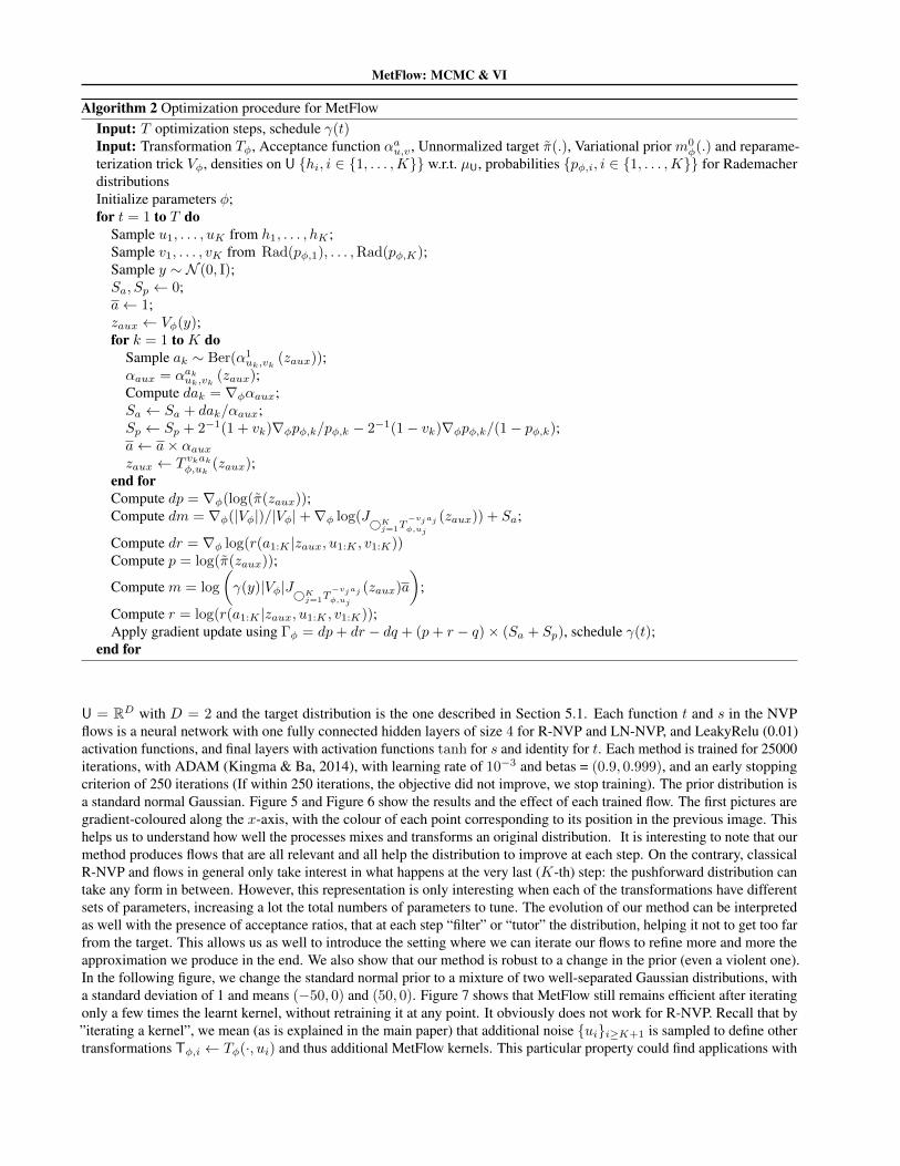
Algorithm 2 Optimization procedure for MetFlowInput: T optimization steps, schedule γ(t)Input: Transformation Tφ, Acceptance function αau,v, Unnormalized target π(.), Variational prior m0
φ(.) and reparame-terization trick Vφ, densities on U {hi, i ∈ {1, . . . ,K}} w.r.t. µU, probabilities {pφ,i, i ∈ {1, . . . ,K}} for RademacherdistributionsInitialize parameters φ;for t = 1 to T do
Sample u1, . . . , uK from h1, . . . , hK ;Sample v1, . . . , vK from Rad(pφ,1), . . . ,Rad(pφ,K);Sample y ∼ N (0, I);Sa, Sp ← 0;a← 1;zaux ← Vφ(y);for k = 1 to K do
Sample ak ∼ Ber(α1uk,vk
(zaux));αaux = αakuk,vk (zaux);Compute dak = ∇φαaux;Sa ← Sa + dak/αaux;Sp ← Sp + 2−1(1 + vk)∇φpφ,k/pφ,k − 2−1(1− vk)∇φpφ,k/(1− pφ,k);a← a× αauxzaux ← T vkakφ,uk
(zaux);end forCompute dp = ∇φ(log(π(zaux));Compute dm = ∇φ(|Vφ|)/|Vφ|+∇φ log(J
©Kj=1T
−vjajφ,uj
(zaux)) + Sa;
Compute dr = ∇φ log(r(a1:K |zaux, u1:K , v1:K))Compute p = log(π(zaux));
Compute m = log
(γ(y)|Vφ|J©K
j=1T−vjajφ,uj
(zaux)a
);
Compute r = log(r(a1:K |zaux, u1:K , v1:K));Apply gradient update using Γφ = dp+ dr − dq + (p+ r − q)× (Sa + Sp), schedule γ(t);
end for
U = RD with D = 2 and the target distribution is the one described in Section 5.1. Each function t and s in the NVPflows is a neural network with one fully connected hidden layers of size 4 for R-NVP and LN-NVP, and LeakyRelu (0.01)activation functions, and final layers with activation functions tanh for s and identity for t. Each method is trained for 25000iterations, with ADAM (Kingma & Ba, 2014), with learning rate of 10−3 and betas = (0.9, 0.999), and an early stoppingcriterion of 250 iterations (If within 250 iterations, the objective did not improve, we stop training). The prior distribution isa standard normal Gaussian. Figure 5 and Figure 6 show the results and the effect of each trained flow. The first pictures aregradient-coloured along the x-axis, with the colour of each point corresponding to its position in the previous image. Thishelps us to understand how well the processes mixes and transforms an original distribution. It is interesting to note that ourmethod produces flows that are all relevant and all help the distribution to improve at each step. On the contrary, classicalR-NVP and flows in general only take interest in what happens at the very last (K-th) step: the pushforward distribution cantake any form in between. However, this representation is only interesting when each of the transformations have differentsets of parameters, increasing a lot the total numbers of parameters to tune. The evolution of our method can be interpretedas well with the presence of acceptance ratios, that at each step “filter” or “tutor” the distribution, helping it not to get too farfrom the target. This allows us as well to introduce the setting where we can iterate our flows to refine more and more theapproximation we produce in the end. We also show that our method is robust to a change in the prior (even a violent one).In the following figure, we change the standard normal prior to a mixture of two well-separated Gaussian distributions, witha standard deviation of 1 and means (−50, 0) and (50, 0). Figure 7 shows that MetFlow still remains efficient after iteratingonly a few times the learnt kernel, without retraining it at any point. It obviously does not work for R-NVP. Recall that by”iterating a kernel”, we mean (as is explained in the main paper) that additional noise {ui}i≥K+1 is sampled to define othertransformations Tφ,i ← Tφ(·, ui) and thus additional MetFlow kernels. This particular property could find applications with

MetFlow: MCMC & VI
Figure 5. Consecutive outputs of each MetFlow kernel. Left: prior normal distribution, then successive effect of the 5 trained MetFlowkernels.
Figure 6. Consecutive outputs of each block of R-NVP. Left: prior normal distribution, then successive effect of the 5 trained R-NVPblocks - 6 transforms each.
time-changing data domains. Indeed, it does not require retraining existing models, while remaining an efficient way tosample from a given distribution at low computational cost.
Figure 7. Changing the prior to a mixture of two separated Gaussians, having trained the method on a standard normal prior. Top row,from left to right: Subsituted prior, 5 trained MetFlow kernels, re-iteration of 100 MetFlow kernels, 200 MetFlow kernels. Bottom row:Substituted prior, R-NVP flow.
In addition to the 2-dimensional results presented in the paper, we show here the results of our method for mixture ofGaussians of higher dimensions. Figure 8 shows the number of Gaussians retrieved by our model when the target distributionis a mixture of 8 Gaussians with variance 1, located at the corners of the d-dimensional hypercube, for different values ofd. We see that our method significantly outperforms others, be they state-of-the-art Normalizing Flows (NAF) or MCMCmethods (NUTS). Furthermore, our method scales more efficiently with dimension, as it is still able to retrieve two of themodes in dim 100 (for some runs), when other methods collapse to one mode for d ≥ 20. MetFlow here is used in thepseudo random setting, with 7 LN-NVP blocks of two elementary transforms, t and s being as previously two one-layerfully connected neural networks, input dimension of twice the dimension considered 2D (again, we take U = RD) andhidden dimension of 2D. The activations functions stay the same. NUTS is ran with 1500 warm-up steps and a length of 10000 samples.

MetFlow: MCMC & VI
Figure 8. Number of modes retrieved by different methods. The target distribution is a mixture of 8 isotropic Gaussian distributions ofvariance 1 located at the corners of a d-dimensional hypercube. The methods are trained to convergence or retrieval of all modes, andmode retrieval is computed by counting the number of samples in a ball of radius 4d around the center of a mode. Error bars represent thestandard deviation of the mean number of modes retrieved for different runs of the method (different initialization and random seed).

MetFlow: MCMC & VI
Figure 9. Density matching for funnel. Top row: Target distribution, MetFlow with 5 trained kernels, MetFlow with 5 trained kerneliterated 100 times. Bottom row: Prior distribution, First run of 5 R-NVP, second run of 5 R-NVP
D.2. Funnel distribution
We now test our approach on an other hard target distribution for MCMC proposed in (Neal, 2003). The target distributionhas density Lebesgue density w.r.t. the Lebesgue measure given for any z ∈ R2 by
π(z) ∝ exp(z21/2) exp(z2ez1/2) . (26)
We are using exactly the same setting for MetFlow with LN-NVP and R-NVP as for the mixture of Gaussian. We train theflows with the same optimizer, for 25000 iterations again. Figure 9 show the results of MetFlow and R-NVP flows. Again,as we are in the pseudo random setting, we sample 95 additional innovation noise (ui)i∈{6,...,100} and show the distributionproduced by 100 MetFlow kernels, having only trained the first five transformations {Tφ,i , i ∈ {1, . . . , 5}}, as described inSection 5 of the main document. We can observe that after only five steps, the distribution has been pushed toward the endof the funnel. However, the amplitude is not recovered fully. It can be interpreted in light of the “tutoring” analogy we usedpreviously. As the Accept/Reject control at each step the evolution of the points, if the number of steps is too small, theproposals do not got to the far end of the distribution. However, the plots show that the proposal given by MetFlow are stilllearnt relevantly, as Figure 9 illustrates that iterating only a few more MetFlow kernels matches the target distribution in allits amplitude.
D.3. Real-world inference - MNIST
In the experiments ran on MNIST described in the main paper, we fix a decoder pθ. To obtain our model, we use the methoddescribed in (Kingma et al., 2016). The mean-field approximation output by the encoder is here pushforward by a flow.In (Kingma et al., 2016), the flows used were Inverse Autoregressive Flows, introduced in the same work. We choose hereto use a more flexible class of flows neural auto-regressive flows (NAF), introduced in (Huang et al., 2018), which show

MetFlow: MCMC & VI
better results in terms of log-likelihood. In practice, we use convolutional networks for our encoder and decoder, matchingthe architecture described in (Salimans et al., 2015). The inference network (encoder) consists of three convolutional layers,each with filters of size 5× 5 and a stride of 2, and output 16, 32, and 32 feature maps, respectively. The output of the thirdlayer feeds a fully connected layer with hidden dimension 450, which then is fully connected to the outputs, means andstandard deviations, of the size of our latent dimension, here 64. Softplus activation functions are used everywhere exceptbefore outputting the means. For the decoder, a similar but reversed architecture is used, using upsampling instead of stride,again as described in (Salimans et al., 2015). The Neural Autoregressive Flows are given by pyro library. NAF have a hiddenlayer of 64 units, with an AutoRegressiveNN which is a deep sigmoidal flow (Huang et al., 2018), with input dimension 64and hidden dimension 128. Our data is the classical stochastic binarization of MNIST (Salakhutdinov & Murray, 2008). Wetrain our model using Adam optimizer for 2000 epoches, using early stopping if there is no improvement after 100 epoches.The learning rate used is 10−3, and betas (0.9, 0.999). This produces a complex and expressive model for both our decoderand variational approximation.
We show first using mixture experiments that MetFlow can overcome state-of-the-art sampling methods. The mixtureexperiment described in the main paper goes as follows. We fix L different samples, and wish to approximate the complexposterior pθ(·|(xi)Li=1)) ∝ p(z)
∏Li=1 pθ(xi|z). We give two approximations of this distribution, given by a state-of-the-art
method, and MetFlow. The state-of-the-art method is a NAF a hidden layer of 16 units, with an AutoRegressiveNN which isa deep sigmoidal flow (Huang et al., 2018), with input dimension 64 and hidden dimension 128. MetFlow is trained here inthe deterministic setting, with 5 blocks of 2 R-NVPs, where again each function t and s is a neural network with one fullyconnected hidden layers of size 128 and LeakyRelu (0.01) activation functions, and final layers with activation functionstanh for s and identity for t. MetFlow and NAF are optimized using 10000 batches of size 250 and early stopping toleranceof 250, with ADAM, with learning rate of 10−3 and betas = (0.9, 0.999). We use Barker ratios as well here. The prior inboth cases is a standard 64-dimensional Gaussian.
Figure 10. Fixed digits for mixture experiment.
Figure 11. Mixture of 3, MetFlow approximation. Figure 12. Mixture of 3, NAF approximation.
We see on Figure 12 that if NAF “collapses” to one fixed digit (thus one specific mode of the posterior), MetFlow Figure 11is able to find diversity and multimodality in the posterior, leading even to “wrong” digits sometimes, showing that it trulyexplores the complicated latent space.
Moreover, we can compare the variational approximations computed for our VAE (encoder - mean field approximation

MetFlow: MCMC & VI
Initial sample MetFlow
Initial sample Encoder
Initial sample Encoder and NAF
Figure 13. Gibbs inpainting experiments starting from digit 0.
Initial sample MetFlow
Initial sample Encoder
Initial sample Encoder and NAF
Figure 14. Gibbs inpainting experiments starting from digit 3.
- and encoder and NAF) to MetFlow approximation. MetFlow used here are the composition of 5 blocks of 2 R-NVPs(deterministic setting), where each function t and s is a neural network with one fully connected hidden layers of size128 and LeakyRelu (0.01) activation functions, and final layers with activation functions tanh for s and identity for t.MetFlow is optimized using 150 epoches of 192 batches of size 250 over the dataset MNIST, with ADAM, with learningrate of 10−4 and betas = (0.9, 0.999) and early stopping with tolerance of 25 (if within 25 epoches the objective did notimprove, we stop training). The optimization goes as follows. We fix encoder (mean-field approximation) and decoder(target distribution). For each sample x in a minibatch of the dataset, we optimize MetFlow starting from the prior given bythe encoder (mean-field approximation) and targetting posterior pθ(·|x). Note that during all this optimization procedure,the initial distribution of MetFlow is fixed to be the encoder, which corresponds to freeze the corresponding parameters.This is a simple generalization of our method to amortized inference. In the following, we use Barker ratios. The additionalresults are given by Figures 13 to 17.
The encoder represents just the mean-field approximation here, while encoder and NAF represent the total variationaldistribution learnt by the VAE described above.
D.4. Additional setting of experiments
So far, we have described two settings. The first one, that we have called deterministic, in which the transformationstake no input “innovation noise”, but all have different sets of parameters. The second one, pseudo random, defines oneglobal transformation Tφ with a unique set of parameters φ, considers K initially sampled at random “innovation noise”u1, . . . , uK , and considers densities h1:K such that the noise resampled at every step of the optimization is “fixed”. It thenlearns the parameters for the global transformation using the considered transformations Tφ,i ← Tφ(·, ui) , i ∈ {1, . . . ,K}.We can consider here a last setting, fully random, on which a global transformation Tφ with a unique set of parametersφ is considered. However, now, we consider a unique density h (typically Gaussian) to sample the “innovation noise” atevery step of the optimization - note that this is still covered by Algorithm C.2. This allow us to consider properly random

MetFlow: MCMC & VI
Initial sample MetFlow
Initial sample Encoder
Initial sample Encoder and NAF
Figure 15. Gibbs inpainting experiments starting from digit 9.
Initial sample MetFlow
Initial sample Encoder
Initial sample Encoder and NAF
Figure 16. Gibbs inpainting experiments starting from digit 6.
Initial sample MetFlow
Initial sample Encoder
Initial sample Encoder and NAF
Figure 17. Gibbs inpainting experiments starting from digit 4.

MetFlow: MCMC & VI
transformations, and looks more like the classical framework of MCMC. Even if this introduces more noise in our stochasticgradient descent, it encourages MetFlow kernels trained to incorporate a lot more diversity. This can be seen with thetwo experiments described before, for mixture of different digits in MNIST, or the inpainting experiments. Even thoughexperiments can show more diversity, it is important to note that they typically require a longer number of epoches to reachconvergence. We give in Appendix D.4 a comparison of the three settings for a mixture of digits problem. As we can see,the diversity introduced by our method is highest in the fully random setting. We can see a wider variety of 3, even thoughother digits tend to appear more when we decode them as well.
Figure 18. Comparison of the different settings described for a mixture of digits experiment. From left to right, deterministic setting,pseudo-random setting, fully random setting.