meta-learning how to forecast time series · 2018-05-07 · meta-learning how to forecast time...

ISSN 1440-771X

Department of Econometrics and Business Statistics

http://business.monash.edu/econometrics-and-business-statistics/research/publications

May 2018

Working Paper 6/18

Meta-learning how to forecast

time series

Thiyanga S Talagala, Rob J Hyndman and George Athanasopoulos



Meta-learning how to forecast time

series

Thiyanga S TalagalaDepartment of Econometrics and Business Statistics,Monash University, VIC 3800, Australia.Email: [email protected] author

Rob J HyndmanDepartment of Econometrics and Business Statistics,Monash University, VIC 3800, Australia.Email: [email protected]

George AthanasopoulosDepartment of Econometrics and Business Statistics,Monash University, VIC 3145, Australia.Email: [email protected]

30 April 2018

JEL classification: C10,C14,C22

mailto:[email protected]



Meta-learning how to forecast time

series

Abstract

A crucial task in time series forecasting is the identification of the most suitable forecasting

method. We present a general framework for forecast-model selection using meta-learning. A

random forest is used to identify the best forecasting method using only time series features.

The framework is evaluated using time series from the M1 and M3 competitions and is

shown to yield accurate forecasts comparable to several benchmarks and other commonly

used automated approaches of time series forecasting. A key advantage of our proposed

framework is that the time-consuming process of building a classifier is handled in advance

of the forecasting task at hand.

Keywords: FFORMS (Feature-based FORecast-model Selection), Time series features,

Random forest, Algorithm selection problem, Classsification

1 Introduction

Forecasting is a key activity for any business to operate efficiently. The rapid advances in

computing technologies have enabled businesses to keep track of large numbers of time

series. Hence, it is becoming increasingly common to have to regularly forecast many

millions of time series. For example, large scale businesses may be interested in forecasting

sales, cost, and demand for their thousands of products across various locations, warehouses,

etc. Technology companies such as Google collect many millions of daily time series such as

web-click logs, web search counts, queries, revenues, number of users for different services,

etc. Such large collections of time series require fast automated procedures generating

accurate forecasts. The scale of these tasks has raised some computational challenges

we seek to address by proposing a new fast algorithm for model selection and time series

forecasting.

Two alternative strategies for generating such a large number of forecasts are: (1) to either

use a single forecasting method across all the time series; or (2) to select an appropriate

forecasting method for each time series individually. It is highly unlikely that a single method

2

Meta-learning how to forecast time series

will consistently outperform judiciously chosen competitor methods across all time series.

We therefore reject the former strategy and focus on an approach for selecting an individual

forecasting method for each time series.

Selecting the most appropriate model for forecasting a given time series can be challenging.

Two of the most commonly used automated algorithms are the exponential smoothing (ets)

algorithm of Hyndman et al. (2002) and the ARIMA (auto.arima) algorithm of Hyndman &

Khandakar (2008). Both algorithms are implemented in the forecast package in R (R Core

Team 2018; Hyndman et al. 2018). In this paradigm, a class of models is selected in advance,

and many models within that class are estimated for each time series. The model with the

smallest AICc value is chosen and used for forecasting. This approach relies on the expert

judgement of the forecaster in first selecting the most appropriate class of models to use, as

it is not usually possible to compare AICc values between model classes due to differences

in the way the likelihood is computed, and the way initial conditions are handled.

An alternative approach, which avoids selecting a class of models a priori, is to use a

simple “hold-out” test set; but then there is often insufficient data to draw a reliable

conclusion. To overcome this drawback, time series cross-validation can be used (Hyndman

& Athanasopoulos 2018); then models from many different classes may be applied, and

the model with the lowest cross-validated MSE selected. However, this increases the

computation time involved considerably (at least to order n2 where n is the number of series

to be forecast).

Clearly, there is a need for a fast and scalable algorithm to automate the process of selecting

models with the aim of forecasting. We refer to this process as forecast-model selection. We

propose a general meta-learning framework using features of the time series to select the

class of models, or even the specific model, to be used for forecasting. The forecast-model

selection process is carried out using a classification algorithm — we use the time series

features as inputs, and the “best” forecasting model as the output. The classifier is built

using a large historical collection of time series, in advance of the forecasting task at hand.

Hence, this is an “offline” procedure.

The “online” process of generating forecasts only involves calculating the features of a time

series and using the pre-trained classifier to identify the best forecasting model. Hence,

generating forecasts only involves the estimation of a single forecasting model, with no

need to estimate large numbers of models within a class, or to carry out a computationally-

Talagala, Hyndman, Athanasopoulos: 30 April 2018 3


intensive cross-validation procedure. We refer to this general framework as FFORMS

(Feature-based FORecast-Model Selection).

The rest of this paper is organized as follows. We review the related work in Section 2. In

Section 3 we explain the detailed components and procedures of our proposed framework

for forecast-model selection. In Section 4 we present the results, followed by the conclusions

and future work in Section 5.

2 Literature review

2.1 Time series features

Rather than work with the time series directly at the level of individual observations, we

propose analysing time series via an associated “feature space”. A time series feature is any

measurable characteristic of a time series. For example, Figure 1 shows the time-domain

representation of six time series taken from the M3 competition (Makridakis & Hibon

2000) while Figure 2 shows a feature-based representation of the same time series. Here

only two features are considered: the strength of seasonality and the strength of trend,

calculated based on the measures introduced by Wang, Smith-Miles & Hyndman (2009).

Time series in the lower right quadrant of Figure 2 are non-seasonal but trended, while there

is only one series with both high trend and high seasonality. We also see how the degree of

seasonality and trend varies between series. Other examples of time series features include

autocorrelation, spectral entropy and measures of self-similarity and nonlinearity. Fulcher &

Jones (2014) identified 9000 operations to extract features from time series.

The choice of the most appropriate set of features depends on both the nature of the time

series being analysed, and the purpose of the analysis. In Section 4, we study the time series

from the M1 and M3 competitions (Makridakis et al. 1982; Makridakis & Hibon 2000), and

we select features for the purpose of forecast-model selection. The M1 and M3 competitions

involve time series of differing length, scale and other properties. We include length as

one of our features, but the remaining features are independent of scale and asymptotically

independent of the length of the time series (i.e., they are ergodic). As our main focus is

forecasting, we select features which have discriminatory power in selecting a good model

for forecasting.



1000

2000

3000

4000

5000

1975 1980 1985

N0001

6000

7000

8000

1975 1980 1985

N0633

2000

3000

4000

1975 1980 1985

N0625

4000

5000

6000

7000

8000

9000

1955 1960 1965 1970 1975 1980 1985

N0645

4000

5000

6000

1982 1984 1986 1988 1990

N1912

2000

3000

4000

5000

1980 1982 1984 1986 1988

N2012

Figure 1: Time-domain representation of time series

N0001

N0633 N0625N0645

N1912

N2012

0.00

0.25

0.50

0.75

1.00

0.00 0.25 0.50 0.75 1.00

trend

seas

onal

ity

Figure 2: Feature-based representation of time series

2.2 What makes features useful for forecast-model selection?

Reid (1972) points out that the performance of forecasting methods changes according to

the nature of the data. Exploring the reasons for these variations may be useful in selecting

the most appropriate model. In response to the results of the M3 competition (Makridakis &

Hibon 2000), similar ideas have been put forward by others. Hyndman (2001), Lawrence

(2001) and Armstrong (2001) argue that the characteristics of a time series may provide



useful insights into which methods are most appropriate for forecasting.

Many time series forecasting techniques have been developed to capture specific character-

istics of time series that are common in a particular discipline. For example, GARCH models

were introduced to account for time-varying volatility in financial time series, and ETS mod-

els were introduced to handle the trend and seasonal patterns which are typical in quarterly

and monthly sales data. An appropriate set of features should reveal the characteristics of

the time series that are useful in determining the best forecasting method.

Several researchers have introduced rules for forecasting based on features (Collopy &

Armstrong 1992; Adya et al. 2001; Wang, Smith-Miles & Hyndman 2009). Most recently

Kang, Hyndman & Smith-Miles (2017) applied principal component analysis to project a

large collection of time series into a two dimensional feature space in order to visualize what

makes a particular forecasting method perform well or not. The features they considered

were spectral entropy, first-order auto-correlation coefficient, strength of trend, strength of

seasonality, seasonal period and the optimal Box-Cox transformation parameter. They also

proposed a method for generating new time series based on specified features.

2.3 Meta-learning for algorithm selection

John Rice was an early and strong proponent of the idea of meta-learning, which he called the

algorithm selection problem (ASP) (Rice 1976). The term meta-learning started to appear

with the emergence of the machine-learning literature. Rice’s framework for algorithm

selection is shown in Figure 3 and comprises four main components. The problem space, P,

represents the data sets used in the study. The feature space, F, is the range of measures

that characterize the problem space P. The algorithm space, A, is a list of suitable candidate

algorithms which can be used to find solutions to the problems in P. The performance metric,

Y, is a measure of algorithm performance such as accuracy, speed, etc. A formal definition

of the algorithm selection problem is given by Smith-Miles (2009), and repeated below.

Algorithm selection problem. For a given problem instance x ∈ P, with

features f (x) ∈ F, find the selection mapping S( f (x)) into algorithm space A,

such that the selected algorithm α ∈ A maximizes the performance mapping

y(α(x)) ∈ Y.

The main challenge in ASP is to identify the selection mapping S from the feature space to the

algorithm space. Even though Rice’s framework articulates a conceptually rich framework,



Figure 3: Rice’s framework for the Algorithm Selection Problem.

it does not specify how to obtain S. This gives rise to the meta-learning approach.

2.4 Forecast-model selection using meta-learning

Selecting models for forecasting can be framed according to Rice’s ASP framework.

Forecast-model selection problem. For a given time series x ∈ P, with fea-

tures f (x) ∈ F, find the selection mapping S( f (x)) into the algorithm space A,

such that the selected algorithm α ∈ A minimizes forecast accuracy error metric

y(α(x)) ∈ Y on the test set of the time series.

Existing methods differ with respect to the way they define the problem space (A), the

features (F), the forecasting accuracy measure (Y) and the selection mapping (S).

Collopy & Armstrong (1992) introduced 99 rules based on 18 features of time series, in

order to make forecasts for economic and demographic time series. This work was extended

by Armstrong (2001) to reduce human intervention.

Shah (1997) used the following features to classify time series: the number of observations,

the ratio of the number of turning points to the length of the series, the ratio of number

of step changes, skewness, kurtosis, the coefficient of variation, autocorrelations at lags

1–4, and partial autocorrelations at lag 2–4. Casting Shah’s work in Rice’s framework, we

can specify: P = 203 quarterly series from the M1 competition (Makridakis et al. 1982);

A = 3 forecasting methods, namely simple exponential smoothing, Holt-Winters exponential

smoothing with multiplicative seasonality, and a basic structural time series model; Y =

mean squared error for a hold-out sample. Shah (1997) learned the mapping S using



discriminant analysis.

Prudêncio & Ludermir (2004) was the first paper to use the term “meta-learning” in the

context of time series model selection. They studied the applicability of meta-learning

approaches for forecast-model selection based on two case studies. Again using the notation

above, we can describe their first case study with: A contained only two forecasting methods,

simple exponential smoothing and a time-delay neural network; Y = mean absolute error; F

consisted of 14 features, namely length, autocorrelation coefficients, coefficient of variation,

skewness, kurtosis, and a test of turning points to measure the randomness of the time

series; S was learned using the C4.5 decision tree algorithm. For their second study, the

algorithm space included a random walk, Holt’s linear exponential smoothing and AR models;

the problem space P contained the yearly series from the M3 competition (Makridakis &

Hibon 2000); F included a subset of features from the first study; and Y was a ranking based

on error. Beyond the task of forecast-model selection, they used the NOEMON approach to

rank the algorithms (Kalousis & Theoharis 1999).

Lemke & Gabrys (2010) studied the applicability of different meta-learning approaches for

time series forecasting. Their algorithm space A contained ARIMA models, exponential

smoothing models and a neural network model. In addition to statistical measures such as

the standard deviation of the de-trended series, skewness, kurtosis, length, strength of trend,

Durbin-Watson statistics of regression residuals, the number of turning points, step changes,

a predictability measure, nonlinearity, the largest Lyapunov exponent, and auto-correlation

and partial-autocorrelation coefficients, they also used frequency domain based features.

The feed forward neural network, decision tree and support vector machine approaches

were considered to learn the mapping S.

Wang, Smith-Miles & Hyndman (2009) used a meta-learning framework to provide recom-

mendations as to which forecast method to use to generate forecasts. In order to evaluate

forecast accuracy, they introduced a new measure Y = simple percentage better (SPB),

which calculates the forecasting accuracy of a method against the forecasting accuracy error

of random walk model. They used a feature set F comprising nine features: strength of trend,

strength of seasonality, serial correlation, nonlinearity, skewness, kurtosis, self-similarity,

chaos and periodicity. The algorithm space A included eight forecast-models, namely, ex-

ponential smoothing, ARIMA, neural networks and random walk model; while the mapping

S was learned using the C4.5 algorithm for building decision trees. In addition, they used



SOM clustering on the features of the time series in order to understand the nature of time

series in a two-dimensional setting.

The set of features introduced by Wang, Smith-Miles & Hyndman (2009) was later used by

Widodo & Budi (2013) to develop a meta-learning framework for forecast-model selection.

The authors further reduced the dimensionality of time series by performing principal

component analysis on the features.

More recently, Kück, Crone & Freitag (2016) proposed a meta-learning framework based

on neural networks for forecast-model selection. Here, P = 78 time series from the NN3

competition were used to build the meta-learner. They introduced a new set of features

based on forecasting errors. The average symmetric mean absolute percentage error was

used to identify the best forecast-models for each series. They classify their forecast-models

in the algorithm space A, comprising single, seasonal, seasonal-trend and trend exponential

smoothing. The mapping S was learned using a feed-forward neural network. Further, they

evaluated the performance of different sets of features for forecast-model selection.

3 Methodology

Our proposed FFORMS framework, presented in Figure 4, builds on this preceding research.

The offline and online phases are shown in blue and red respectively. A classification

algorithm (the meta-learner) is trained during the offline phase and is then used to select an

appropriate forecast model for a new time series in the online phase.

In order to train our classification algorithm, we need a large collection of time series which

are similar to those we will be forecasting. We assume that we have an essentially infinite

population of time series, and we take a sample of them in order to train the classification

algorithm denoted as the “observed sample”. The new time series we wish to forecast can

be thought of as additional draws from the same population. Hence, any conclusions made

from the classification framework refer only to the population from which the sample has

been selected. We may call this the “target population” of time series. It is important to have

a well-defined target population to avoid misapplying the classification rules. In practice, we

may wish to augment the set of observed time series by simulating new time series similar

to those in the assumed population (we provide details and discussion in Section 3.1 that

follows). We denote the total collection of time series used for training the classifier as the

“reference set”. Each time series within the reference set is slit into a training period and



Figure 4: FFORMS (Feature-based FORecast-Model Selection) framework. The offline phase isshown in blue and the online phase by red.

a test period. From each training period we compute a range of time series features, and

fit a selection of candidate models. The calculated features form the input vector to the

classification algorithm. Using the fitted models, we generate forecasts and identify the

“best” model for each time series based on a forecast error measure (e.g., MASE) calculated

over the test period. The models deemed “best” form the output labels for the classification

algorithm. The pseudo code for our proposed framework is presented in Algorithm 1 below.

In the following sections, we briefly discuss aspects of the offline phase.

3.1 Augmenting the observed sample with simulated time series

In practice, we may wish to augment the set of observed time series by simulating new

time series similar to those in the assumed population. This process may be useful when

the number of observed time series is too small to build a reliable classifier. Alternatively,

we may wish to add more of some particular types of time series to the reference set in

order to get a more balanced sample for the classification. In order to produce simulated

series that are similar to those in the population, we consider two classes of data generating

processes: exponential smoothing models and ARIMA models. Using the automated ets and

auto.arima algorithms (Hyndman et al. 2018) we identify models, based on model selection

criteria (such as AICc) and simulate multiple time series from the selected models within



Algorithm 1 The FFORMS framework - Forecasting based on meta-learning.

Offline phase - train the classifierGiven:

O = {x1, x2, . . . , xn} : the collection of n observed time series.L : the set of class labels (e.g. ARIMA, ETS, SNAIVE).F : the set of functions to calculate time series features.nsim : number of series to be simulated.B : number of trees in the random forest.f : number of features to be selected at each node.

Output:FFORMS classifier

Prepare the reference setFor i = 1 to n:

1: Fit ARIMA and ETS models to xi.2: Simulate nsim time series from each model in step 1.3: The time series in O and simulated time series in step 2 form the reference set R ={x1, x2, . . . , xn, xn+1, . . . , xN} where N = n + nsim.

Prepare the meta-dataFor j = 1 to N:

4: Split xj into a training period and test period.5: Calculate features F based on the training period.6: Fit L models to the training period.7: Calculate forecasts for the test period from each model.8: Calculate forecast error measure over the test period for all models in L.9: Select the model with the minimum forecast error.

10: Meta-data: input features (step 5), output labels (step 9).

Train a random forest classifier11: Train a random forest classifier based on the meta-data.12: Random forest: the ensemble of trees {Tb}B

1 .

Online phase - forecast a new time seriesGiven:

FFORMS classifier from step 12 .Output:

class labels for new time series xnew.13: For xnew calculate features F.14: Let Cb(xnew) be the class prediction of the bth random forest tree. Then class label for

xnew is Cr f (xnew) = majorityvote{Cb(xnew)}B1 .

each model class. Assuming the models produce data that are similar to the observed time

series ensures that the simulated series are similar to those in the population. As this is done

in the offline phase of the algorithm the computational time in producing these simulated

series is of no real consequence.



3.2 Input: features

Our proposed FFORMS algorithm requires features that enable identification of a suitable

forecast model for a given time series. Therefore, the features used should capture the

dynamic structure of the time series, such as trend, seasonality, autocorrelation, nonlinearity,

heterogeneity, and so on. Furthermore, interpretability, robustness to outliers, scale and

length independence should also be considered when selecting features for this classification

problem. A comprehensive description of the features used in the experiment is presented

in Table 2.

A feature of the proposed FFORMS framework is that its online phase is fast compared to

the time required for implementing a typical model selection or cross-validation procedure.

Therefore, we consider only features that can be computed rapidly, as this computation must

be done during the online phase.

3.3 Output: labels

The task of the classification algorithm is to identify the “best” forecasting method for a

given time series. It is not possible to train the classifier for all possible classes of models.

However, we should consider enough possibilities so that the algorithm can be used for

forecast-model selection with some confidence. The candidate models considered as labels

will depend on the observed time series. For example, if we have only non-seasonal time

series, and no chaotic features, we may wish to restrict the models to white noise, random

walk, ARIMA and ETS processes. Even in this simple scenario, the number of possible

models can be quite large.

Each candidate model considered is estimated strictly on the training period of each series

in the reference set. Forecasts are then generated for the test period over which the chosen

forecast accuracy measure is calculated. The model with the lowest forecast error measure

over the test period is deemed “best”.

This step is the most computationally intensive and time-consuming, as each candidate model

has to be applied on each series in the reference set. However, as this task is done during

the offline phase of the FFORMS framework, the time involved and computational cost

associated are of no real significance and are completely controlled by the user. The more

candidate models that are considered as labels, the more computational time is required;



however the pay-off could be significant gains in forecast accuracy.

3.4 Random forest algorithm

A random forest (Breiman 2001) is an ensemble learning method that combines a large num-

ber of decision trees using a two-step randomization process. Let (y1, z1), (y2, z2), . . . , (yN , zN)

represent the reference set, where input yi is an m-vector of features, output zi corresponds

to the class label of the ith time series, and N is the number of series in the reference set.

Each tree in the forest is grown based on a bootstrap sample of size N from the reference

set. At each node of the tree, randomly select f < m features from the full set of features.

The best split is selected among those f features. The split which results in the most

homogeneous subnodes is considered the best split. Various measures have been introduced

to evaluate the homogeneity of subnodes, such as classification error rate, the Gini index

and cross entropy (Friedman, Hastie & Tibshirani 2009). In this study, we use the Gini index

to evaluate the homogeneity of a particular split. The trees are grown to the largest extent

possible without pruning. To determine the class label for a new instance, features are

calculated and passed down the trees. Then each tree gives a prediction and the majority

vote over all individual trees leads to the final decision. In this work, we have used the

randomForest package (Liaw & Wiener 2002; Breiman et al. 2018) which implements the

Fortran code for random forest classification by Breiman & Cutler (2004).

4 Application to the M competition data

To test how well our proposed framework can identify suitable models for forecasting, we

use the yearly, quarterly and monthly series from the M1 (Makridakis et al. 1982) and M3

competitions (Makridakis & Hibon 2000). The R package Mcomp (Hyndman 2018) provides

the data for both these. We run two experiments. In the first experiment, we treat the

time series from the M1 competition as the observed sample and the time series from the

M3 competition as the new time series to be forecast. We reverse the sets in the second

experiment, treating the M3 data as the observed sample and the M1 data as the new time

series. The experimental set-ups are summarised in Table 1. These allow us to compare our

results with published forecast accuracy results for each of these competitions.

In each experiment, we fit ARIMA and ETS models to the full length of each series in the

corresponding observed samples using the auto.arima and ets functions in the forecast



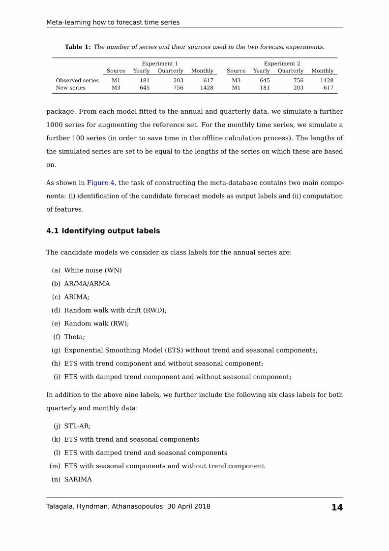
Table 1: The number of series and their sources used in the two forecast experiments.

Experiment 1 Experiment 2Source Yearly Quarterly Monthly Source Yearly Quarterly Monthly

Observed series M1 181 203 617 M3 645 756 1428New series M3 645 756 1428 M1 181 203 617

package. From each model fitted to the annual and quarterly data, we simulate a further

1000 series for augmenting the reference set. For the monthly time series, we simulate a

further 100 series (in order to save time in the offline calculation process). The lengths of

the simulated series are set to be equal to the lengths of the series on which these are based

on.

As shown in Figure 4, the task of constructing the meta-database contains two main compo-

nents: (i) identification of the candidate forecast models as output labels and (ii) computation

of features.

4.1 Identifying output labels

The candidate models we consider as class labels for the annual series are:

(a) White noise (WN)

(b) AR/MA/ARMA

(c) ARIMA;

(d) Random walk with drift (RWD);

(e) Random walk (RW);

(f) Theta;

(g) Exponential Smoothing Model (ETS) without trend and seasonal components;

(h) ETS with trend component and without seasonal component;

(i) ETS with damped trend component and without seasonal component;

In addition to the above nine labels, we further include the following six class labels for both

quarterly and monthly data:

(j) STL-AR;

(k) ETS with trend and seasonal components

(l) ETS with damped trend and seasonal components

(m) ETS with seasonal components and without trend component

(n) SARIMA



(o) Seasonal naive method.

Most of these are self-explanatory labels based on models implemented in the forecast

package using the default settings.

STL-AR refers to forecasts based on an STL decomposition applied to the time series, then an

AR model is used to forecast the seasonally adjusted data, while the seasonal naive method

is used to forecast the seasonal component. The two sets of forecasts are then combined to

provide forecasts on the original time scale (Hyndman & Athanasopoulos 2018).

For each series in the reference set, all candidate models are estimated using the training

period, and forecasts are generated for the whole of the test period as set by the competitions.

The model corresponding to the smallest MASE (Hyndman & Koehler 2006) calculated over

the test period is selected as the “best model” and forms the output label for that series.

4.2 Feature computation process

We use a set of 25 features for yearly data and a set of 30 features for seasonal data. Some

of these are taken from previous studies (Wang, Smith-Miles & Hyndman 2009; Hyndman,

Wang & Laptev 2015; Kang, Hyndman & Smith-Miles 2017), and we have also added new

features that we believe provide some useful information. Each feature can be computed

rapidly, thus making the online phase of our algorithm extremely fast. The features are

summarized in Table 2, and fully described in the Appendix.

Correlation matrices for all the features calculated from the reference sets of each of the

experiments are presented in Figure 5. The variability in the correlations reflects the

diversity of the selected features. In other words, the features we have employed seem

to capture different characteristics of the time series. Furthermore, the structure of the

correlation matrices across the same frequencies of the two experiments seem to be fairly

similar. This sends a strong signal that the M1 and M3 collections of time series may have

similar feature spaces.

4.3 Model calibration

The random forest (RF) algorithm is highly sensitive to class imbalance (Breiman 2001),

and our reference set is unbalanced: some classes contain significantly more cases than

other classes. The degree of class imbalance is reduced to some extent by augmenting the

observed sample with the simulated time series. We consider three approaches to address



Figure 5: Correlation matrix plots for the reference sets.



Table 2: Features used for selecting a forecast-model.

Feature Description Non-seasonal Seasonal

1 T length of time series X X2 trend strength of trend X X3 seasonality strength of seasonality - X4 linearity linearity X X5 curvature curvature X X6 spikiness spikiness X X7 e_acf1 first ACF value of remainder series X X8 stability stability X X9 lumpiness lumpiness X X10 entropy spectral entropy X X11 hurst Hurst exponent X X12 nonlinearity nonlinearity X X13 alpha ETS(A,A,N) α X X14 beta ETS(A,A,N) β X X15 hwalpha ETS(A,A,A) α - X16 hwbeta ETS(A,A,A) β - X17 hwgamma ETS(A,A,A) γ - X18 ur_pp test statistic based on Phillips-Perron test X -19 ur_kpss test statistic based on KPSS test X -20 y_acf1 first ACF value of the original series X X21 diff1y_acf1 first ACF value of the differenced series X X22 diff2y_acf1 first ACF value of the twice-differenced series X X23 y_acf5 sum of squares of first 5 ACF values of original series X X24 diff1y_acf5 sum of squares of first 5 ACF values of differenced series X X25 diff2y_acf5 sum of squares of first 5 ACF values of twice-differenced series X X26 seas_acf1 autocorrelation coefficient at first seasonal lag - X27 sediff_acf1 first ACF value of seasonally-differenced series - X28 sediff_seacf1 ACF value at the first seasonal lag of seasonally-differenced

series- X

29 sediff_acf5 sum of squares of first 5 autocorrelation coefficients ofseasonally-differenced series

- X

30 lmres_acf1 first ACF value of residual series of linear trend model X -31 y_pacf5 sum of squares of first 5 PACF values of original series X X32 diff1y_pacf5 sum of squares of first 5 PACF values of differenced series X X33 diff2y_pacf5 sum of squares of first 5 PACF values of twice-differenced

seriesX X

the class imbalance in the data: (1) incorporating class priors into the RF classifier; (2) using

the balanced RF algorithm introduced by Chen, Liaw & Breiman (2004); and (3) re-balancing

the reference set with down-sampling. In down-sampling, the size of the reference set is

reduced by down-sampling the larger classes so that they match the smallest class in size;

this potentially discards some useful information. Comparing the results, the balanced RF

algorithm and RF with down-sampling did not yield satisfactory results. We therefore only

report the results obtained by the RF built on unbalanced data (RF-unbalanced) and the RF

with class priors (RF-class priors). The RF algorithms are implemented by the randomForest

R package (Liaw & Wiener 2002; Breiman et al. 2018). The class priors are introduced

through the option classwt. We use the reciprocal of class size as the class priors. The

number of trees ntree is set to 1000, and the number of randomly selected features f is set



to be one third of the total number of features available.

Our aim is different from most classification problems in that we are not interested in

accurately predicting the class, but in finding the best possible forecast model. It is possible

that two models produce almost equally accurate forecasts, and therefore it is not important

whether the classifier picks one model over the other. Therefore we report the forecast

accuracy obtained from the FFORMS framework, rather than the classification accuracy.

4.4 Summary of the main results

We build separate RF classifiers for yearly data, quarterly data and monthly data. For the

second experiment (for which data from the M3 competition are the observed series), in the

case of yearly and quarterly data we take a subset of the simulated time series when training

the RF-unbalanced and RF-class priors, to reduce the size of the reference set (these are

shown in yellow in the figures that follow). The subsets are selected randomly according to

the proportions of output labels in the observed samples. This ensures that our reference

set shares similar characteristics to the observed sample.

We use principal component analysis to visualize the feature-spaces of the different time

series collections. We compute the principal components projection using the features in the

observed sample, and then project the simulated time series and the new time series using

the same projection. The results are shown in Figures 6–7, where the first three principal

components are plotted against each other. Figure 6 refers to Experiment 1 and Figure 7 to

Experiment 2. The points on each plot represent individual time series. In each figure the

first column of plots refers to the yearly data, the middle column to the quarterly data and

the last column to the monthly data. The plots show that the first three principle components

explain 62.5%, 62.4% and 58.9% of the total variation in the yearly, quarterly and monthly

M1 data and 62.2% 64.7% and 66.0% of the total variation in the yearly, quarterly and

monthly M3 data.

The plots show that the distribution of the observed time series over the PCA space (repre-

sented by the black dots) is very similar to that of the new time series (represented by the

orange dots). More importantly, we see that the distribution of the simulated time series

(represented by the green dots and yellow dots - the yellow dots are a subset of the simulated

series as mentioned above) clearly nests and fills in the space of the new time series. Further,

in both experiments, all the observed time series fall within the space of all simulated data.



Figure 6: Experiment 1: Distribution of time series in the PCA space. Distribution of yearly seriesare shown in the first column, distribution of quarterly series are shown in the secondcolumn, and the distribution of monthly series are shown in the third column. On eachgraph, green indicates simulated time series, black indicates observed time series, whileorange denotes new time series.

This strongly indicates that we have not reduced the feature diversity from the observed

sample. By augmenting the observed series with simulated time series, we have been able

to increase the diversity and evenness of the feature space in the reference sets.

We compare the accuracy of the forecasts generated from the FFORMS framework to the

following commonly-used forecasting methods:

1. automated ARIMA algorithm of Hyndman & Khandakar (2008);

2. automated ETS algorithm of Hyndman & Khandakar (2008);

3. Random walk with drift (RWD);



Figure 7: Experiment 2: Distribution of time series in the PCA space. Distribution of yearly seriesare shown in the first column, distribution of quarterly series are shown in the secondcolumn, and the distribution of monthly series are shown in the third column. On eachgraph, green indicates simulated time series, yellow shows a subset of simulated timeseries, black indicates observed time series, while orange denotes new time series.

4. Random walk model (RW);

5. White noise process (WN);

6. Theta method;

7. STL-AR method (for seasonal data);

8. seasonal naive (for seasonal data).

The automated ARIMA and ETS algorithms are implemented using the auto.arima and

ets functions available in the forecast package in R. Each method is implemented on the

training period of the new series and forecasts are computed for the full length of the test

period. This follows closely the forecast evaluation process implemented in the M1 and M3



forecasting competitions. The MASE is computed for each forecast horizon, by averaging

the absolute scaled forecast errors across all series. The rank is calculated by averaging

the ranks of each competing method across all forecast horizons and series. The results are

presented in Table 3. The lowest MASE and average rank values corresponding to the best

performing method are presented in bold font.

Table 3: MASE values calculated over the new series for Experiments 1 and 2.

Experiment 1: new series M3 Experiment 2: new series M1

Yearly Yearlyh = 1 1− 2 1− 4 1− 6 Rank h = 1 1− 2 1− 4 1− 6 Rank

RF-unbalanced 1.06 1.40 2.17 2.82 3.50 0.98 1.40 2.43 3.39 1.50RF-class priors 1.04 1.38 2.15 2.79 2.50 1.01 1.40 2.43 3.38 1.50auto.arima 1.11 1.48 2.28 2.96 5.83 1.06 1.47 2.51 3.47 3.33ets 1.09 1.44 2.20 2.86 4.67 1.12 1.59 2.72 3.77 5.00WN 6.54 6.91 7.48 8.07 9.00 6.38 7.08 8.59 10.01 8.00RW 1.24 1.68 2.48 3.17 8.00 1.35 2.00 3.50 4.89 7.00RWD 1.03 1.36 2.05 2.63 1.00 1.04 1.44 2.51 3.49 3.67Theta 1.12 1.47 2.18 2.77 3.50 1.15 1.70 3.00 4.19 6.00

Quarterly Quarterlyh = 1 1− 4 1− 6 1− 8 Rank h = 1 1− 4 1− 6 1− 8 Rank

RF-unbalanced 0.59 0.81 0.97 1.12 2.25 0.74 1.08 1.35 1.57 1.00RF-class priors 0.59 0.82 0.97 1.13 3.13 0.76 1.12 1.40 1.62 2.63auto.arima 0.59 0.85 1.02 1.19 4.75 0.78 1.17 1.50 1.74 5.25ets 0.56 0.82 0.99 1.17 3.75 0.78 1.11 1.42 1.66 3.00WN 3.25 3.59 3.70 3.87 10.00 3.97 4.27 4.45 4.64 10.00RW 1.14 1.16 1.32 1.46 7.00 0.97 1.35 1.67 1.95 7.50RWD 1.20 1.17 1.36 1.47 6.50 0.95 1.26 1.56 1.81 5.38STL-AR 0.70 1.27 1.60 1.91 8.34 0.96 1.63 2.05 2.43 8.63Theta 0.62 0.83 0.97 1.11 2.50 0.79 1.13 1.42 1.67 3.88Snaive 1.11 1.09 1.30 1.43 6.75 1.52 1.56 1.87 2.08 7.75

Monthly Monthlyh = 1 1− 6 1− 12 1− 18 Rank h = 1 1− 6 1− 12 1− 18 Rank

RF-unbalanced 0.60 0.68 0.76 0.87 3.22 0.61 0.76 0.90 1.03 1.77RF-class priors 0.60 0.67 0.75 0.86 2.00 0.60 0.75 0.92 1.06 2.83auto.arima 0.55 0.64 0.74 0.87 2.83 0.60 0.76 0.96 1.12 4.94ets 0.55 0.64 0.74 0.86 2.72 0.59 0.76 0.93 1.07 3.44WN 2.01 2.08 2.15 2.27 10.00 1.93 2.09 2.18 2.28 10.00RW 0.84 0.97 1.04 1.17 8.03 1.05 1.24 1.33 1.47 7.25RWD 0.84 0.96 1.02 1.14 6.89 1.06 1.27 1.39 1.55 8.61STL-AR 0.64 0.81 1.04 1.27 7.89 0.63 0.91 1.17 1.39 7.38Theta 0.58 0.67 0.77 0.89 4.22 0.61 0.75 0.92 1.04 2.27Snaive 0.95 0.97 0.99 1.15 7.19 1.06 1.11 1.14 1.31 6.47

In general, our proposed FFORMS meta-learning algorithm performs quite well in both

experimental settings. It consistently ranks in the top most accurate forecasting methods

for forecasting both the M1 and the M3 series and most often ranks as the most accurate

method. For yearly data, FFORMS ranks best for forecasting the M1 data in experiment 2

and second (to the random walk with drift) in forecasting the M3 data. For quarterly data,

FFORMS ranks as the most accurate in both experiments. For monthly data, FFORMS seems



to perform best for the longer horizons in both experimental settings. It also seems to be

competitive for the shorter horizons with the three methods (auto.arima, ets and theta)

that perform best. Comparing the results across the two experimental settings, it seems that

using the FFORMS algorithm achieves marginally better results in experiment 2. Hence,

this indicates that the meta-learning algorithm benefits from being trained on the larger

observed sample of time series (M3 series) while forecasting a smaller new set (M1 series).

5 Discussion and conclusions

In this paper we have proposed a novel framework for forecast-model selection using

meta-learning based on time series features. Our proposed FFORMS algorithm uses the

knowledge of the past performance of candidate forecast models on a collection of time

series in order to identify the best forecasting method for a new series. We have shown that

the method almost always performs better than common benchmark methods, and in many

cases better than the best-performing methods from both the M1 and the M3 forecasting

competitions. Although we have illustrated the method using the M1 and M3 competition

data, the framework is general and can be applied to any large collection of time series.

A major advantage of the FFORMS framework is that the classifier is trained offline and

selecting a forecasting model for a new time series is as fast as calculating a set of features

and passing these to the pretrained classifier. Therefore, unlike traditional model selection

strategies or cross-validation processes, our proposed framework can be used to accurately

forecast very large collections of time series requiring almost instant forecasts.

In addition to our new FFORMS framework, we have also introduced a simple set of time

series features that are useful in identifying the “best” forecast method for a given time

series, and can be computed rapidly. We will leave to a later study an analysis of which of

these features are the most useful, and how our feature set could be reduced further without

the loss of forecast accuracy.

For real-time forecasting, our framework involves only the calculation of features, the

selection of a forecast method based on the FFORMS random forest classifier, and the

calculation of the forecasts from the chosen model. None of these steps involve substantial

computation, and they can be easily parallelised when forecasting for a large number of new

time series. For future work, we will explore the use of other classification algorithms within

the FFORMS algorithm, and test our approach on several other large collections of time



series.

Appendix: Definition of features

Length of time series

The appropriate forecast method for a time series depends on how many observations are

available. For example, shorter series tend to need simple models such as a random walk.

On the other hand, for longer time series, we have enough information to be able to estimate

a number of parameters. For even longer series (over 200 observations), models with

time-varying parameters give good forecasts as they help to capture the changes of the

model over time.

Features based on an STL-decomposition

The strength of trend, strength of seasonality, linearity, curvature, spikiness and first

autocorrelation coefficient of the remainder series, are calculated based on a decomposition

of the time series. Suppose we denote our time series as y1, y2, . . . , yT. First, an automated

Box-Cox transformation (Guerrero 1993) is applied to the time series in order to stabilize

the variance and to make the seasonal effect additive. The transformed series is denoted

by y∗t . For quarterly and monthly data, this is decomposed using STL (Cleveland, Cleveland

& Terpenning 1990) to give y∗t = Tt + St + Rt, where Tt denotes the trend, St denotes the

seasonal component, and Rt is the remainder component. For non-seasonal data, Friedman’s

super smoother (Friedman 1984) is used to decompose y∗t = Tt + Rt, and St = 0 for all t. The

de-trended series is y∗t − Tt = St + Rt, the deseasonalized series is y∗t − St = Tt + Rt..

The strength of trend is measured by comparing the variance of the deseasonalized series

and the remainder series (Wang, Smith-Miles & Hyndman 2009):

Trend = max [0, 1− Var(Rt)/Var(Tt + Rt)] .

Similarly, the strength of seasonality is computed as

Seasonality = max [0, 1− Var(Rt)/Var(St + Rt)] .

The linearity and curvature features are based on the coefficients of an orthogonal quadratic



regression

Tt = β0 + β1φ1(t) + β2φ2(t) + εt,

where t = 1, 2, . . . , T, and φ1 and φ2 are orthogonal polynomials of orders 1 and 2. The

estimated value of β1 is used as a measure of linearity while the estimated value of β2

is considered as a measure of curvature. These features were used by Hyndman, Wang

& Laptev (2015). The linearity and curvature depend on the the scale of the time series.

Therefore, the time series are scaled to mean zero and variance one before these two

features are computed.

The spikiness feature is useful when a time series is affected by occasional outliers. Hyndman,

Wang & Laptev (2015) introduced an index to measure spikiness, computed as the variance

of the leave-one-out variances of rt.

We compute the first autocorrelation coefficient of the remainder series, rt.

Stability and lumpiness

The features “stability” and “lumpiness” are calculated based on tiled windows (i.e., they do

not overlap). For each window, the sample mean and variance are calculated. The stability

feature is calculated as the variance of the means, while lumpiness is the variance of the

variances. These were first used by Hyndman, Wang & Laptev (2015).

Spectral entropy of a time series

Spectral entropy is based on information theory, and can be used as a measure of the

forecastability of a time series. Series that are easy to forecast should have a small spectral

entropy value, while very noisy series will have a large spectral entropy. We use the measure

introduced by Goerg (2013) to estimate the spectral entropy. It estimates the Shannon

entropy of the spectral density of the normalized spectral density, given by

Hs(yt) := −∫ π

−πfy(λ) log fy(λ)dλ,

where fy denotes the estimate of the spectral density introduced by Nuttall & Carter (1982).

The R package ForeCA (Goerg 2016) was used to compute this measure.



Hurst exponent

The Hurst exponent measures the long-term memory of a time series. The Hurst expo-

nent is given by H = d + 0.5, where d is the fractal dimension obtained by estimating a

ARFIMA(0, d, 0) model. We compute this using the maximum likelihood method (Haslett &

Raftery 1989) as implemented in the fracdiff package (Fraley 2012). This measure was also

used in Wang, Smith-Miles & Hyndman (2009).

Nonlinearity

To measure the degree of nonlinearity of the time series, we use statistic computed in

Terasvirta’s neural network test for nonlinearity (Teräsvirta, Lin & Granger 1993), also

used in Wang, Smith-Miles & Hyndman (2009). This takes large values when the series is

nonlinear, and values around 0 when the series is linear.

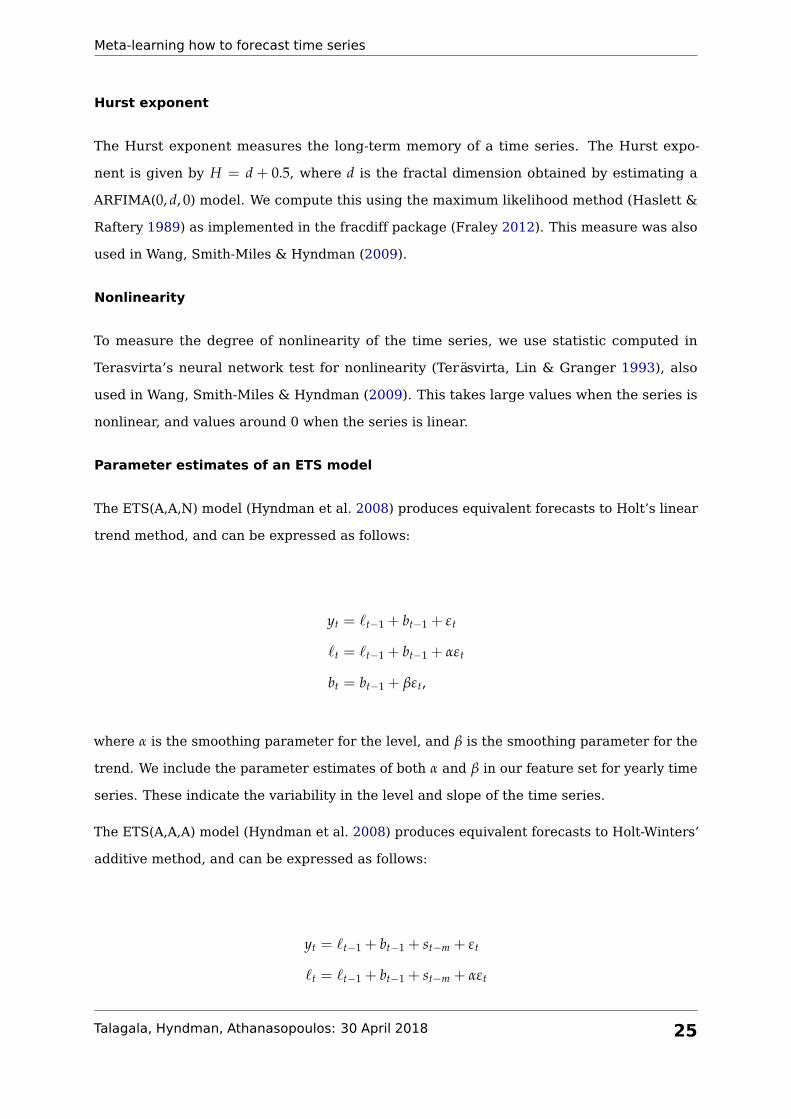
Parameter estimates of an ETS model

The ETS(A,A,N) model (Hyndman et al. 2008) produces equivalent forecasts to Holt’s linear

trend method, and can be expressed as follows:

yt = `t−1 + bt−1 + εt

`t = `t−1 + bt−1 + αεt

bt = bt−1 + βεt,

where α is the smoothing parameter for the level, and β is the smoothing parameter for the

trend. We include the parameter estimates of both α and β in our feature set for yearly time

series. These indicate the variability in the level and slope of the time series.

The ETS(A,A,A) model (Hyndman et al. 2008) produces equivalent forecasts to Holt-Winters’

additive method, and can be expressed as follows:

yt = `t−1 + bt−1 + st−m + εt

`t = `t−1 + bt−1 + st−m + αεt



bt = bt−1 + βεt,

st = st−m + γεt,

where γ is the smoothing parameter for the seasonal component, and the other parameters

are as above. We include the parameter estimates of α, β and γ in our feature set for monthly

and quarterly time series. The value of γ provides a measure for the variability of the

seasonality of a time series.

Unit root test statistics

The Phillips-Perron test is based on the regression yt = c + αyt−1 + εt. The test statistic we

use as a feature is the usual “Z-alpha” statistic with the Bartlett window parameter set to

the integer value of 4(T/100)0.25 (Pfaff 2008). This is the default value returned from the

ur.pp() function in the urca package (Pfaff, Zivot & Stigler 2016).

The KPSS test is based on the regression yt = c + δt + αyt−1 + εt. The test statistic we use as

a feature is the usual KPSS statistic with the Bartlett window parameter set to the integer

value of 4(T/100)0.25 (Pfaff 2008). This is the default value returned from the ur.kpss()

function in the urca package (Pfaff, Zivot & Stigler 2016).

Autocorrelation coefficient based features

We calculate the first-order autocorrelation coefficient and the sum of squares of the first

five autocorrelation coefficients of the original series, the first-differenced series, the second-

differenced series, and the seasonally differenced series (for seasonal data).

A linear trend model is fitted to the time series, and the first-order autocorrelation coefficient

of the residual series is calculated.

We calculate the sum of squares of the first five partial autocorrelation coefficients of the

original series, the first-differenced series and the second-differenced series.

References

Adya, M, F Collopy, JS Armstrong & M Kennedy (2001). Automatic identification of time

series features for rule-based forecasting. International Journal of Forecasting 17(2),

143–157.



Armstrong, JS (2001). Should we redesign forecasting competitions? International Journal of

Forecasting 17(1), 542–543.

Breiman, L (2001). Random forests. Machine Learning 45(1), 5–32.

Breiman, L & A Cutler (2004). Random Forests. Version 5.1. https://www.stat.berkeley.

edu/~breiman/RandomForests/.

Breiman, L, A Cutler, A Liaw & M Wiener (2018). randomForest: Breiman and Cutler’s

Random Forests for Classification and Regression. R package version 4.6-14. https:

//cran.r-project.org/web/packages/randomForest/.

Chen, C, A Liaw & L Breiman (2004). Using random forest to learn imbalanced data. Tech.

rep. University of California, Berkeley. http://statistics.berkeley.edu/sites/

default/files/tech-reports/666.pdf.

Cleveland, RB, WS Cleveland & I Terpenning (1990). STL: A seasonal-trend decomposition

procedure based on loess. Journal of Official Statistics 6(1), 3.

Collopy, F & JS Armstrong (1992). Rule-based forecasting: development and validation of an

expert systems approach to combining time series extrapolations. Management Science

38(10), 1394–1414.

Fraley, C (2012). fracdiff: Fractionally differenced ARIMA aka ARFIMA(p,d,q) models. R

package version 1.4-2. https://CRAN.R-project.org/package=fracdiff.

Friedman, JH (1984). A variable span scatterplot smoother. Technical Report 5. Laboratory

for Computational Statistics, Stanford University.

Friedman, J, T Hastie & R Tibshirani (2009). The elements of statistical learning. 2nd ed.

New York, USA: Springer.

Fulcher, BD & NS Jones (2014). Highly comparative feature-based time-series classification.

IEEE Transactions on Knowledge and Data Engineering 26(12), 3026–3037.

Goerg, GM (2016). ForeCA: An R package for forecastable component analysis. R package

version 0.2.4. https://CRAN.R-project.org/package=ForeCA.

Goerg, G (2013). Forecastable component analysis. In: Proceedings of the 30th International

Conference on Machine Learning (ICML-13), pp.64–72.

Guerrero, VM (1993). Time-series analysis supported by power transformations. Journal of

Forecasting 12, 37–48.

Haslett, J & AE Raftery (1989). Space-time modelling with long-memory dependence: As-

sessing Ireland’s wind power resource. Applied Statistics 38(1), 1–50.


https://www.stat.berkeley.edu/~breiman/RandomForests/

https://www.stat.berkeley.edu/~breiman/RandomForests/

https://cran.r-project.org/web/packages/randomForest/

https://cran.r-project.org/web/packages/randomForest/

http://statistics.berkeley.edu/sites/default/files/tech-reports/666.pdf

http://statistics.berkeley.edu/sites/default/files/tech-reports/666.pdf

https://CRAN.R-project.org/package=fracdiff

https://CRAN.R-project.org/package=ForeCA


Hyndman, RJ (2001). It’s time to move from what to why. International Journal of Forecasting

17(1), 567–570.

Hyndman, RJ (2018). Mcomp: Data from the M-Competitions. R package version 2.7. https:

//CRAN.R-project.org/package=Mcomp.

Hyndman, RJ & G Athanasopoulos (2018). Forecasting: principles and practice. 2nd ed.

Melbourne, Australia: OTexts. https://OTexts.org/fpp2/.

Hyndman, RJ & Y Khandakar (2008). Automatic time series forecasting: the forecast package

for R. Journal of Statistical Software 26(3), 1–22.

Hyndman, RJ & AB Koehler (2006). Another look at measures of forecast accuracy. Interna-

tional Journal of Forecasting 22(4), 679–688.

Hyndman, RJ, AB Koehler, JK Ord & RD Snyder (2008). Forecasting with exponential

smoothing: the state space approach. Berlin: Springer.

Hyndman, RJ, AB Koehler, RD Snyder & S Grose (2002). A state space framework for

automatic forecasting using exponential smoothing methods. International Journal of

Forecasting 18(3), 439–454.

Hyndman, RJ, E Wang & N Laptev (2015). Large-scale unusual time series detection. In: Data

Mining Workshop (ICDMW), 2015 IEEE International Conference on. IEEE, pp.1616–

1619.

Hyndman, R, G Athanasopoulos, C Bergmeir, G Caceres, L Chhay, M O’Hara-Wild, F Petropou-

los, S Razbash, E Wang & F Yasmeen (2018). forecast: Forecasting functions for time se-

ries and linear models. R package version 8.3. http://pkg.robjhyndman.com/forecast.

Kalousis, A & T Theoharis (1999). NOEMON: Design, implementation and performance

results of an intelligent assistant for classifier selection. Intelligent Data Analysis 3(5),

319–337.

Kang, Y, RJ Hyndman & K Smith-Miles (2017). Visualising forecasting algorithm performance

using time series instance spaces. International Journal of Forecasting 33(2), 345–358.

Kück, M, SF Crone & M Freitag (2016). Meta-learning with neural networks and landmarking

for forecasting model selection an empirical evaluation of different feature sets applied

to industry data. In: Neural Networks (IJCNN), 2016 International Joint Conference on.

IEEE, pp.1499–1506.

Lawrence, M (2001). Why another study? International Journal of Forecasting 17(1), 574–

575.


https://CRAN.R-project.org/package=Mcomp

https://CRAN.R-project.org/package=Mcomp

https://OTexts.org/fpp2/

http://pkg.robjhyndman.com/forecast


Lemke, C & B Gabrys (2010). Meta-learning for time series forecasting and forecast combi-

nation. Neurocomputing 73(10), 2006–2016.

Liaw, A & M Wiener (2002). Classification and regression by randomForest. R News 2(3),

18–22.

Makridakis, S, A Andersen, R Carbone, R Fildes, M Hibon, R Lewandowski, J Newton, E

Parzen & R Winkler (1982). The accuracy of extrapolation (time series) methods: results

of a forecasting competition. Journal of forecasting 1(2), 111–153.

Makridakis, S & M Hibon (2000). The M3-Competition: results, conclusions and implications.

International Journal of Forecasting 16(4), 451–476.

Nuttall, AH & GC Carter (1982). Spectral estimation using combined time and lag weighting.

Proceedings of the IEEE 70(9), 1115–1125.

Pfaff, B (2008). Analysis of integrated and cointegrated time series with R. Springer.

Pfaff, B, E Zivot & M Stigler (2016). urca: Unit root and cointegration tests for time series

data. R package version 1.3-0. https://CRAN.R-project.org/package=urca.

Prudêncio, RB & TB Ludermir (2004). Meta-learning approaches to selecting time series

models. Neurocomputing 61, 121–137.

R Core Team (2018). R: A Language and Environment for Statistical Computing. R Foundation

for Statistical Computing. Vienna, Austria. https://www.R-project.org/.

Reid, DJ (1972). “A comparison of forecasting techniques on economic time series”. In:

Forecasting in Action. Birmingham, UK: Operational Research Society.

Rice, JR (1976). The algorithm selection problem. Advances in Computers 15, 65–118.

Shah, C (1997). Model selection in univariate time series forecasting using discriminant

analysis. International Journal of Forecasting 13(4), 489–500.

Smith-Miles, K (2009). Cross-disciplinary perspectives on meta-learning for algorithm selec-

tion. ACM Computing Surveys (CSUR) 41(1), 6.

Teräsvirta, T, CF Lin & CWJ Granger (1993). Power of the neural network linearity test.

Journal of Time Series Analysis 14 (2), 209–220.

Wang, X, K Smith-Miles & RJ Hyndman (2009). Rule induction for forecasting method

selection: meta-learning the characteristics of univariate time series. Neurocomputing

72(10), 2581–2594.

Widodo, A & I Budi (2013). “Model selection using dimensionality reduction of time series

characteristics”. Paper presented at the International Symposium on Forecasting, Seoul,

South Korea. June 2013. https://goo.gl/ig2J57.


https://CRAN.R-project.org/package=urca

https://www.R-project.org/

https://goo.gl/ig2J57

meta-learning how to forecast time series · 2018-05-07 · meta-learning how to forecast time...

Documents