meshless method for simulation of compressible flow

UNLV Theses, Dissertations, Professional Papers, and Capstones

August 2017

Meshless Method for Simulation of Compressible Flow Meshless Method for Simulation of Compressible Flow

Ebrahim Nabizadeh Shahrebabak University of Nevada, Las Vegas

Follow this and additional works at: https://digitalscholarship.unlv.edu/thesesdissertations

Part of the Aerospace Engineering Commons, and the Mechanical Engineering Commons

Repository Citation Repository Citation Nabizadeh Shahrebabak, Ebrahim, "Meshless Method for Simulation of Compressible Flow" (2017). UNLV Theses, Dissertations, Professional Papers, and Capstones. 3092. http://dx.doi.org/10.34917/11156761

This Thesis is protected by copyright and/or related rights. It has been brought to you by Digital Scholarship@UNLV with permission from the rights-holder(s). You are free to use this Thesis in any way that is permitted by the copyright and related rights legislation that applies to your use. For other uses you need to obtain permission from the rights-holder(s) directly, unless additional rights are indicated by a Creative Commons license in the record and/or on the work itself. This Thesis has been accepted for inclusion in UNLV Theses, Dissertations, Professional Papers, and Capstones by an authorized administrator of Digital Scholarship@UNLV. For more information, please contact [email protected].

http://library.unlv.edu/

http://library.unlv.edu/

https://digitalscholarship.unlv.edu/thesesdissertations

https://digitalscholarship.unlv.edu/thesesdissertations?utm_source=digitalscholarship.unlv.edu%2Fthesesdissertations%2F3092&utm_medium=PDF&utm_campaign=PDFCoverPages

http://network.bepress.com/hgg/discipline/218?utm_source=digitalscholarship.unlv.edu%2Fthesesdissertations%2F3092&utm_medium=PDF&utm_campaign=PDFCoverPages

http://network.bepress.com/hgg/discipline/293?utm_source=digitalscholarship.unlv.edu%2Fthesesdissertations%2F3092&utm_medium=PDF&utm_campaign=PDFCoverPages

http://dx.doi.org/10.34917/11156761

mailto:[email protected]

MESHLESS METHOD FOR SIMULATION OF COMPRESSIBLE FLOW

By

Ebrahim Nabizadeh Shahrebabak

Bachelor of Science- Chemical Engineering

Isfahan University of Technology, Iran

2014

A thesis submitted in partial fulfillment

of the requirements for the

Master of Science - Mechanical Engineering

Department of Mechanical Engineering

Howard R. Hughes College of Engineering

The Graduate College

University of Nevada, Las Vegas

August 2017

ii

Thesis Approval

The Graduate College The University of Nevada, Las Vegas

June 28, 2017

This thesis prepared by


entitled

Meshless Method for Simulation of Compressible Flow

is approved in partial fulfillment of the requirements for the degree of

Master of Science - Mechanical Engineering Department of Mechanical Engineering

Darrell W. Pepper, Ph.D. Kathryn Hausbeck Korgan, Ph.D. Examination Committee Chair Graduate College Interim Dean Dr. Hui Zhao, Ph.D. Examination Committee Member William Culbreth, Ph.D. Examination Committee Member Laxmi Gewali, Ph.D. Graduate College Faculty Representative

iii

ABSTRACT

In the present age, rapid development in computing technology and high speed

supercomputers has made numerical analysis and computational simulation more practical than

ever before for large and complex cases. Numerical simulations have also become an essential

means for analyzing the engineering problems and the cases that experimental analysis is not

practical. There are so many sophisticated and accurate numerical schemes, which do these

simulations. The finite difference method (FDM) has been used to solve differential equation

systems for decades. Additional numerical methods based on finite volume and finite element

techniques are widely used in solving problems with complex geometry. All of these methods

are mesh-based techniques. Mesh generation is an essential preprocessing part to discretize the

computation domain for these conventional methods. However, when dealing with mesh-based

complex geometries these conventional mesh-based techniques can become troublesome,

difficult to implement, and prone to inaccuracies. In this study, a more robust, yet simple

numerical approach is used to simulate problems in an easier manner for even complex problem.

The meshless, or meshfree, method is one such development that is becoming the focus

of much research in the recent years. The biggest advantage of meshfree methods is to

circumvent mesh generation. Many algorithms have now been developed to help make this

method more popular and understandable for everyone. These algorithms have been employed

over a wide range of problems in computational analysis with various levels of success. Since

there is no connectivity between the nodes in this method, the challenge was considerable. The

most fundamental issue is lack of conservation, which can be a source of unpredictable errors in

the solution process. This problem is particularly evident in the presence of steep gradient

iv

regions and discontinuities, such as shocks that frequently occur in high speed compressible flow

problems.

To solve this discontinuity problem, this research study deals with the implementation of

a conservative meshless method and its applications in computational fluid dynamics (CFD).

One of the most common types of collocating meshless method the RBF-DQ, is used to

approximate the spatial derivatives. The issue with meshless methods when dealing with highly

convective cases is that they cannot distinguish the influence of fluid flow from upstream or

downstream and some methodology is needed to make the scheme stable. Therefore, an

upwinding scheme similar to one used in the finite volume method is added to capture steep

gradient or shocks. This scheme creates a flexible algorithm within which a wide range of

numerical flux schemes, such as those commonly used in the finite volume method, can be

employed. In addition, a blended RBF is used to decrease the dissipation ensuing from the use of

a low shape parameter. All of these steps are formulated for the Euler equation and a series of

test problems used to confirm convergence of the algorithm.

The present scheme was first employed on several incompressible benchmarks to validate

the framework. The application of this algorithm is illustrated by solving a set of incompressible

Navier-Stokes problems.

Results from the compressible problem are compared with the exact solution for the flow

over a ramp and compared with solutions of finite volume discretization and the discontinuous

Galerkin method, both requiring a mesh. The applicability of the algorithm and its robustness are

shown to be applied to complex problems.

v

ACKNOWLEDGMENTS

I would like to express my profound gratitude to my academic advisor, Prof.

Darrell Pepper, for his scholastic advice and technical guidance throughout this investigation.

His devotion, patience, and focus on excellence allowed me to reach this important milestone in

my life. I also wish to extend my acknowledgements to the examination committee members, Dr.

William Culbreth, Dr. Hui Zhao, and Dr. Laxmi Gewali for their guidance and suggestions.

vi

DEDICATION

This study is dedicated to my wife, Farideh, and my parents, Khadijeh and Azizollah.

Without their continued and unconditional love and support, I would not be the person I am

today.

vii

TABLE OF CONTENTS

ABSTRACT ............................................................................................................................... iii

ACKNOWLEDGMENTS ........................................................................................................... v

LIST OF TABLES ...................................................................................................................... x

LIST OF FIGURES .................................................................................................................... xi

CHAPTER 1- INTRODUCTION ........................................................................................... 1

Previous research studies ................................................................................................. 1

Motivation ........................................................................................................................ 2

Objective .......................................................................................................................... 4

Thesis Outline .................................................................................................................. 6

CHAPTER 2- RADIAL BASIS FUNCTIONS ....................................................................... 7

Introduction ...................................................................................................................... 7

Shape parameter ............................................................................................................. 10

Global RBF .................................................................................................................... 11

Localized RBF ................................................................................................................ 12

RBF-DQ ......................................................................................................................... 14

Summery ........................................................................................................................ 16

CHAPTER 3- APPLICATION OF RBF-DQ TO SOLVE INCOMPRESSIBLE FLOW .... 18

Introduction .................................................................................................................... 18

Flow Solution ................................................................................................................. 18

Governing Equations .............................................................................................. 18

Projection Method ................................................................................................... 19

viii

Benchmarks Examination .............................................................................................. 21

Moving Wall Cavity ............................................................................................... 22

3.3.1.1. Problem setup .................................................................................................. 22

3.3.1.2. Localized RBF-DQ .......................................................................................... 22

Natural Convection inside a close square ............................................................... 23

3.3.2.1. Problem setup .................................................................................................. 23

3.3.2.2. Localized RBF-DQ .......................................................................................... 23

Flow with Forced Convection over a Backward-Facing Step ................................ 24

3.3.3.1. Problem setup .................................................................................................. 24

3.3.3.2. Localized RBF-DQ .......................................................................................... 25

Summery ........................................................................................................................ 25

CHAPTER 4- RBF-DQ FOR COMPRESSIBLE FLOW ..................................................... 28

Introduction .................................................................................................................... 28

The Euler Equations ....................................................................................................... 28

Conservation-Law Form ......................................................................................... 30

RBF-DQ Implementation ............................................................................................... 31

Upwinding Scheme ........................................................................................................ 33

Roe’s approximate Riemann solver ........................................................................ 34

Summery ........................................................................................................................ 39

CHAPTER 5- COMPERISSIBLE FLOW BENCHMARK.................................................. 41

Benchmark Problem ....................................................................................................... 41

Problem domain ...................................................................................................... 41

Boundary conditions ............................................................................................... 43

ix

Effect of parameters ....................................................................................................... 47

Shape parameter ...................................................................................................... 47

Size of subdomain ................................................................................................... 47

Slope limiter ............................................................................................................ 47

Time step ................................................................................................................. 48

Postprocessing ................................................................................................................ 49

CHAPTER 6- CONCLUSION AND FUTURE WORK ...................................................... 53

Summary of work ........................................................................................................... 53

Future work .................................................................................................................... 54

APPENDIX: NOMENCLATURE................................................................................................ 55

REFERENCES ............................................................................................................................. 56

CURRICULUM VITAE ............................................................................................................... 60

x

LIST OF TABLES

Table 3.1 Constant parameter of each case ................................................................................... 19

Table 5.1 Inlet condition ............................................................................................................... 46

xi

LIST OF FIGURES

Figure 2.1 Size of subdomain a) 9 node stencil, b) 15 node stencil, c) 20 node stencil ............... 14

Figure 3.1 Cavity problem: Velocity vector plots of two scheme for Re=100. a) Present Scheme,

b) Reference scheme (Waters & Pepper, 2015) ............................................................................ 23

Figure 3.2 Natural convection: Velocity Vector plots of two scheme for Pr=0.71, and Ra=103. a)

Present scheme, b) Reference scheme (Waters & Pepper, 2015) ................................................. 26

Figure 3.3 Natural convection: Temperature contours of two schemes for distribution with

Pr=0.71, Ra=103. a) Present scheme, b) Reference scheme (Waters & Pepper, 2015) ............... 26

Figure 3.4 Backward facing: Streamline for fluid flow. a) Present scheme, b) Reference scheme

(Waters & Pepper, 2015) .............................................................................................................. 27

Figure 3.5 Backward facing: isothermal for fluid flow. a) Present scheme, b) Reference scheme

(Waters & Pepper, 2015) .............................................................................................................. 27

Figure 4.1 Configuration in subdomain ........................................................................................ 32

Figure 4.2 Position of conservative variables ............................................................................... 37

Figure 4.3 Present algorithm flowchart ........................................................................................ 40

Figure 5.1 Benchmark domain ...................................................................................................... 42

Figure 5.2 Node distribution ......................................................................................................... 42

Figure 5.3 Configuration in subdomain ........................................................................................ 42

Figure 5.4 Wall boundary condition ............................................................................................. 44

Figure 5.5 Mach number contour .................................................................................................. 50

Figure 5.6 Pressure contour .......................................................................................................... 50

Figure 5.7 Pressure contour using Finite Volume Method ........................................................... 51

Figure 5.8 Pressure contour using DG Method ............................................................................ 51

xii

Figure 5.9 Exact solution (Wang & Widhopf, 1989) .................................................................... 52

Figure 5.10 Pressure along the bottom wall.................................................................................. 52

1

CHAPTER 1- INTRODUCTION

Natural phenomena, whether electrical, biological, mechanical, chemical, environmental,

geological or electronic, can be described by means of mathematical models. Since most of these

problems are complex, it is hard to find exact solutions for these models. The way to find

solutions for these problems is to solve them numerically or statistically. Nowadays, researchers

have to be familiar with numerical or statistical techniques for a wide variety of problems. By

the advent of supercomputer technology, computational simulation techniques have increasingly

become an essential way for simulating complex and practical problems in engineering and

science where experimental analysis is highly expensive.

The main purpose of numerical simulation is to discretize the continuum physical domain

to a discretized domain which is solvable on computers. The discretization process is applied to

both equations and the domain of the problem. Researchers can find an approximate solution for

a complex problem efficiently, as long as a proper and reliable numerical method is

implemented.

Previous research studies

Many studies have focused on numerical or approximation methods to develop an

efficient technique. Many numerical methods have been proposed and developed, utilizing the

finite difference method (FDM), the finite volume method (FVM), the finite element method

(FEM), the boundary element method (BEM), and more recently the meshless method to be

discussed here.

2

Studies on meshless methods can be traced back to 1977, but only a few studies had been

done in this area until the past two decades. Lucy (1977), using one of the oldest forms of the

meshless method, smooth particle hydrodynamics (SPH), modeled astrophysical phenomenon.

More recently, a wide range of meshless methods have been developed and studied. Such

improved methods includ the smooth particle hydrodynamics (SPH) (Gingold & Monaghan,

1977; Lucy, 1977; Monaghan, 1988; Randles & Libersky, 1996), the diffuse element method

(DEM) (Nayroles, Touzot, & Villon, 1992), the element free Galerkin (EFG) method

(Belytschko, Lu, & Gu, 1994; Lu, Belytschko, & Gu, 1994; Noguchi, Kawashima, & Miyamura,

2000), the reproducing kernel particle method (RKPM), the moving least-squares reproducing

kernel (MLSRK) method (Liu, Jun, Li, Adee, & Belytschko, 1995), the hp-clouds method

(Duarte & Oden, 1996; Liszka, Duarte, & Tworzydlo, 1996), the finite point method (Onate,

Idelsohn, Zienkiewicz, Taylor, & Sacco, 1996), the meshless local Petrov-Galerkin (MLPG)

method (Atluri & Zhu, 1998), boundary node method (BNM) (Mukherjee & Mukherjee, 1997),

the meshless local boundary integral equation (MLBIE) method (Atluri & Zhu, 2000), and the

gridless Euler/Navier–Stokes solution (Batina, 1993; Morinishi, 1995). Another group of

meshless methods, are based on radial basis functions (RBFs). More recently, RBFs have

become attractive for solving partial differential equations. The RBF methods for multivariate

approximation have wide applications in modern approximation theory when the task is to

approximate scattered data in several dimensions.

Motivation

For decades, the finite element method (FEM) and the finite volume method (FVM) have

been the standards tool for numerically solving a wide variety of engineering problems

3

especially fluid flow and thermal problem simulation. However, as problems become more

complex, these methods become inadequate and inefficient. A good mesh is very important in

CFD. This can be an expensive issue in the sense of storage needed and CPU time, especially

when dealing with complex geometries and/or complex physics such as crack propagation, shock

propagation, astrophysics phenomena, metal cutting and extrusion. Conventional methods

always have some difficulties when they are used to solve these kinds of problems. Therefore, to

get accurate results, a highly dense mesh near the discontinuity is usually required; otherwise, the

computational results are not reliable.

Using conventional methods can cause some degradation of accuracy in complex physics,

since adaptive meshing in conventional methods is difficult to implement. On the other hand, it

is impractical to solve system containing billions of unknowns. The time and cost of mesh

generation and mesh refinement in conventional methods is high.

To reduce the cost of the meshing process, different methods have been proposed over

the past three decades and a significant progress has been achieved in this area. Like all the

previous techniques, the governing equations of essential parameters like mass, momentum, and

energy must be conserved by each these new techniques One of the promising numerical

techniques to satisfy all these limitations is the meshless, or meshfree method.

Engineering research has began focusing the use of meshless method, over the past

decade. Since meshless methods eliminate the mesh generation required for discretization of

problem domains, the approximation process only needs to collocate a functional value on

distributed set of nodes. The connection between nodes is not required, which helps reduce

4

storage. Time can also be saved by using a fully automated procedure to generate nodes (G. R.

Liu, 2010).

The use of meshless methods can lead to computational advantages with less

programming efforts; especially a hybrid meshless method in combination with a conventional

method can improve the result for complicated “multiphysics” problems. Some of the advantages

of meshless are :

1) Computational cost is reduced and storage saved significantly since a mesh and book

keeping are not required.

2) For cases where more refinement is needed, one can easily increase the accuracy by

using r-adaptation or adding nodes to the computational domain. Providing high-

order shape functions are constructed.

3) The Meshless routine can be used many time during the solving process.

Objective

Compared to conventional FDM, FVM, and FEM, the meshless method can be used to

track strong discontinuities or large deformations of strongly nonlinear problems. To increase the

resolution near geometric complexities, one can add nodes and refine the simulation. This makes

the programing and simulation more convenient to solve complex system of equations over

arbitrary domains.

There are different ways to distribute the nodes throughout the domain. One can use any

type of uniform, nonuniform or hybrid distribution to collocate the data. The dependency of

conventional methods on the mesh causes some problems in refinement processes near a

5

discontinuity. Thus, they are not very suitable and applicable for tracking discontinuities such as

shocks or strong deformation, especially when they are not aligned with the original mesh edges

(Belytschko, Krongauz, Organ, Fleming, & Krysl, 1996). The common procedure for solving a

moving or evolving discontinuity in conventional techniques is to remesh the simulation field in

each iteration. The remeshing process can be a source of numerous difficulties such as reduction

of accuracy and cumbersome programming. Moreover, successive remeshing processes can also

be a significant waste in terms of the computational time and cost. On the other hand, the

meshless methods does not significantly require mesh dependency processes. The goal of

meshless methods is to remove the mesh related problems by performing approximations over all

the nodes. Therefore, moving deformation or discontinuity propagation can be tracked without

remeshing, with little compromise in accuracy. Since the refinement process is easier in

meshless, this degradation in accuracy can be compensated by performing refinement around the

discontinuities.

In the present study a blended localized Radial Basis Function Differential Quadrature

(RBF-DQ) for solving the Euler equation is introduced. The algorithm is blended to three

different regions and include a steep gradient limitation for the shape parameter, which changes

to high and low values. The derivatives are approximated using RBF-DQ, and will be explained

later. The other essential part of the study is dealing with the discontinuities and capturing shock

propagation. An upwinding scheme is applied to compute the fluxes at the mid-point between the

reference point and the support point. Roe’s solver which is an approximate Riemann solver is

used in this study. The conservative values at the each side of the mid-point approximated by

using blended RBF-DQ and then the fluxes are computed.

6

Thesis Outline

The scheme is examined for several incompressible and compressible cases with

discontinuities. In the chapter 2, an introduction to RBF and more details about the aspects of

RBF are provided. In chapter 3, we test the RBF-DQ code on several incompressible flow

problems and compare with flow benchmarks obtained from other studies. Some details about

the setup process are also provided. Chapter 4 introduce the Euler equation and its hyperbolic

characteristics. The details of Roe’s scheme, which is used here for the purpose of upwinding, is

described. The blended RBF-DQ is introduced and the idea of blending explained. In chapter 5,

we obtain results for supersonic flow with an oblique shock throughout the domain. The results

are in a good agreement with the exact solution. The method is also compared qualitatively and

quantitatively with several other numerical schemes and in some cases, the results are more

accurate. In addition, the dependency of different parameters on the accuracy of the solution such

as uniform or nonuniform distribution of nodes and value of shape parameter and timestep are

also discussed. Chapter 6 provides the conclusions drawn from this study and suggestions for

future research in the area of RBF approximation.

7

CHAPTER 2- RADIAL BASIS FUNCTIONS

Introduction

Radial basis function methods are the means to approximate the multivariate functions

we wish to study in this section. This type of truly meshfree interpolation begins with the idea

that any arbitrary domain, especially irregular domains can be approximated by collocating about

a number of nodes distributed in the domain with some set of basis functions. There are two

types of RBF approximation, global meshless method and local meshless method. The former

method solves the domain by using a large sparse matrix that is calculated from all the nodes

inside the domain. This type of approximation has some well-known drawbacks, which will be

discussed later. For the second method, one needs to divide the overall domain into a number of

smaller subdomains, which leads to more effective and precise results when compared to global

approximation. The size of the subdomain includes a predetermined number of the nearest nodes

surrounding the reference point. The accuracy of the solution relies on many parameters such as

the number of supporting nodes and their distribution and the value of the shape parameter.

Formulation and details of these methods follow.

RBFs were initially developed for multivariate scatter data and function interpolation.

The meshfree feature of RBFs on higher dimensional problems motivated researchers to employ

them in solving PDEs. After some research, they found that this type of meshfree approximation

has high-order accuracy than conventional finite difference schemes on a scattered distribution of

nodes (Tota, 2006). Due to the simplicity of programming and small amount storage required,

researchers began to use them in all area of numerical modeling.

8

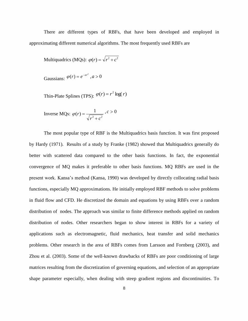
There are different types of RBFs, that have been developed and employed in

approximating different numerical algorithms. The most frequently used RBFs are

Multiquadrics (MQs): 22)( crr

Gaussians:

2

)( arer 0, a

Thin-Plate Splines (TPS): )log()( 2 rrr

Inverse MQs: 22

1)(

crr

0, c

The most popular type of RBF is the Multiquadrics basis function. It was first proposed

by Hardy (1971). Results of a study by Franke (1982) showed that Multiquadrics generally do

better with scattered data compared to the other basis functions. In fact, the exponential

convergence of MQ makes it preferable to other basis functions. MQ RBFs are used in the

present work. Kansa’s method (Kansa, 1990) was developed by directly collocating radial basis

functions, especially MQ approximations. He initially employed RBF methods to solve problems

in fluid flow and CFD. He discretized the domain and equations by using RBFs over a random

distribution of nodes. The approach was similar to finite difference methods applied on random

distribution of nodes. Other researchers began to show interest in RBFs for a variety of

applications such as electromagnetic, fluid mechanics, heat transfer and solid mechanics

problems. Other research in the area of RBFs comes from Larsson and Fornberg (2003), and

Zhou et al. (2003). Some of the well-known drawbacks of RBFs are poor conditioning of large

matrices resulting from the discretization of governing equations, and selection of an appropriate

shape parameter especially, when dealing with steep gradient regions and discontinuities. To

9

overcome the first issue, some preconditioning and domain decomposition technique is required

(Ling & Kansa, 2005; Mai-Duy & Tran-Cong, 2002). This is the reason for better performance

of localized meshless method over global meshless.

The solution for these problems will be discussed later. Wu and Shu (2002) developed a

new branch of differential quadrature, which is fully mesh-free. This type of DQ uses radial basis

functions as the approximation functions and the nodes inside each sub domain are used to

approximate partial derivatives at a reference node. Shu et al. (2003) proposed a local RBF-based

differential quadrature (RBF-DQ) method. They applied RBF-DQ for simulation of

incompressible flow problems. There are also some pioneer studies on using RBFs for capturing

socks and discontinuities. Shu et al. (2005) used RBF-DQ with an upwinding scheme to capture

the shock waves and compressible flow simulation. The method is fully mesh-free but due to the

small value of shape parameter, shocks are smeared. Harris el at. (2017) implemented a blended

RBFs scheme where the shape parameter switches to high and low value according to the

gradient region. Low value was used for steep gradient regions and higher values in smooth

regions.

The framework of this current meshfree approach is formed of three parts: the first part is

the derivative approximation by the means of localized RBF-DQ method; then blend the

approximation depending on the position of the node by changing the shape parameter; the last

step is the meshfree upwinding scheme for flux calculation.

In the following sections, we will introduce the global and localized RBF method. In

addition, details about localized DQ-RBF will be provided later.

10

Shape parameter

The shape parameter is a key factor in RBFs approximation when using MQ and inverse

MQ. Choosing an irrelevant number can create an inaccurate solution. It has a positive real value

less than one. There is no theory and proven analysis of how to select the shape parameter to

obtain the most accurate result. Wang and Liu (2002) investigated the effect of the shape

parameter for MQ and Gaussian basis function. They found that for MQ basis, the condition

number of the matrix is stable when the shape parameter is less than 1. They also showed that a

high shape parameter increases the condition number. Another study, has carried out by Frank

and Schaback (1998), examined the RBF method to solve partial derivatives equations and

derived a formula for choosing the shape parameter as

IN

Rc

25.1

where NI is the size of the subdomain and R is the radius of the smallest subdomain. Hardy

(1971) introduced another formula for estimating the shape parameter:

dc 815.0

where d is calculated by

1

1

i

iI

dN

d with di being the distance between the reference node

and the other nodes in the subdomain. Afiatdoust and Esmaeilbeigi (2015) also examined an

algorithm to find the optimal value of the shape parameter, and showed some improvement in the

accuracy of the simulations. Their proposed algorithm make a balance between accuracy and ill-

condition and obtain desirable accuracy only for solving ODEs. The algorithm is time-

consuming and its cost of calculation is high.

11

Global RBF

Consider the general differential equation

)(xfLu in , )(xgBu on 2.1

where L can be any arbitrary differential operator, B is an operator imposed on the boundaries

and can be any kind of boundary condition, such as Dirichlet, Neumann, or Robin condition. Let

N

iii xP1

be N collocation points in the analyzed domain, where IN

iix1are interior nodes and

N

NiiI

x1are boundary points. Kansa (1990) suggested the following approximation for Eq.

(2.1)

)()( xuxu j

N

ij

j

2.2

where N

ju 1 are the summation of unknowns and boundary values and )()( jj PPx is the

radial basis function. IN

ju 1 are the unknown coefficients to be determined, N

Nj Iu 1 are the

boundary values which needed to be fixed after each iteration. For MQ RBFs, jPPr is the

Euclidean distance between nodes P=(x) and Pj=(xj). For each point (xj,yj), j is calculated by

the following expression

222 )()()( cyyxxx jjj 2.3

Substituting Eq. (2.1) into Eq. (2.2), leads to an N×N linear system of equations,

12

)())((1

jjjj

N

j

xfuxL

, j=0,1,2,…,NI 2.4

)())((1

jjjj

N

j

xguxB

, j= 1NN ,2IN ,…, N 2.5

in which we just solve for the interior nodes. Therefore, a matrix of NI×NI Eq. (2.1), for the

unknown IN

iix1 needs to be solved. In order to approximate each governing equation, there is a

NI×NI linear system to be solved in each iteration, as NI denotes all the interior nodes. Random

distribution of nodes can increase the condition number of the matrices and consequently leading

to ill-conditioning and a source of instability. The idea of using the meshless method is to

preform simulations on PC-Level creating huge matrices is not applicable in this situation. The

solution can be highly expensive when large matrices need to be inverted. In addition, the global

RBF meshless method is applicable for small and regular domains but is not practical for large

complex geometries or/and physics involving many nodes.

Localized RBF

The second type of RBF approximation is the localized meshless method. The drawbacks arising

from the global meshless method can be largely overcome by using the localized meshless

method. In fact, the idea of localized RBF interpolation starts with the concept that any irregular

domain can be interpolated by doing collocation about a small number of nodes in each

subdomains. The basis functions are calculated utilizing local points in each subdomain. Using

subdomains to approximate a set of unknowns result in a more efficient and accurate solution

method when compared to global interpolation techniques. To create the subdomains, for each

interior node Pj , we assign a subdomain including m nearest nodes in the subdomain of

13

influence m

kjj P 1, . Here the reference node is marked Pj, while the index k changes between 1 to

m consisting of the reference point itself. Fig. (2.1) shows different subdomain stencils for 9, 15

and 20 nodes. The reference point and its supporting points j

Ix , j =1, 2... m are identified by the

red color.

Once again, consider Eq. (2.1). To approximate the function or its derivatives, we can use

support domains instead of the whole domain. Here, the function value, u, can be interpolated as:

)()( xuxu j

m

ij

j

in j 2.6

and the differential operator L, can be calculated as

)())((1

jjjj

m

j

xfuxL

in j 2.7

where the subdomain j is a small domain surrounding the reference point. Comparing Eq. (2.6)

with Eq. (2.2) we see that the only difference in formulation is the size of the matrix, i.e., N×N

versus a small matrix of m×m. This feature of the localized meshless method has some attractive

advantages such as parallel processing capability (because of the presence of subdomains), easy

calculation of the matrix inversion, and the ability for a fully independent approach at the

problem setup stage.

14

Figure 2.1 Size of subdomain a) 9 node stencil, b) 15 node stencil, c) 20 node stencil

RBF-DQ

In this section, the formulation of the Localized RBF differential quadrature, LRBFDQ,

method is given. In this method, the function is approximated by RBFs and all the derivatives are

approximated by differential quadrature (DQ). Therefore, the derivative of the function at the

reference point is interpolated by a weighted linear sum of function values at a number of

discrete nodes inside its subdomain. It should be noted that these weight coefficients are only a

function of the space between the distributed nodes. Shu el at. (2003) showed that the weighting

c

a b

15

coefficients can be easily computed utilizing a linear vector space and a function approximation.

In this study the unknown function )(xf is approximated by the linear combination of the

multiquadrics (MQs). As mentioned before, they are the most accurate basis function among

various RBF-based interpolation methods. It should be noted that in the localized RBF-DQ

method, the subdomain at other nodes are different. The size of the subdomain can also be

changed, making the method more flexible. For example, the approximation of the mth order

derivative of a function f(x) at the node xI by RBF-DQ can be expressed as

IN

j

j

I

m

jIm

m

xfwx

f

0

, )( , j=0,1,2,…,NI 2.6

)( j

Ixf = function values at the distributed points

m

jIw , =RBF-DQ weight coefficients at the points

where j

Ix are the positions of supporting point Ix , and II xx 0 .The symbol IN shows the number

of supporting nodes within the subdomain of the reference point Ix . For simplicity of notation

)(xwk is used to replace )( kk xxw , where kxx is the Euclidean distance.

According to the principle of superposition, all the basis functions should satisfy the relation

described in Eq. (2.6) , i.e. expressed in matrix form as

m

iN

m

i

m

i

NNNN

N

N

iN

i

i

m

m

w

w

w

xxx

xxx

xxx

x

x

x

x

2

1

21

22212

12111

2

1

)(

)()()(

)()()(

)()()(

)(

)(

)(

2.7

From Eq. (2.3), one can easily obtain the first order derivative of 1

1

x

i

as:

16

2221

1

)()(

),(

cyyxx

xx

x

yx

jiji

jiiik

2.8

In a similar manner, the weighting coefficients of the y-derivatives can also be computed.

Also, one can obtain the second and higher order derivatives of )(x by differentiating Eq. (2.3)

successively. The second derivative can be expressed as

3222

22

2

2

))()((

)(),(

cyyxx

cxx

x

yx

jiji

jiiik

2.9

Since the weighting coefficients are based on the local position of supporting points in

the subdomains, this approach is very suitable in dealing with nonlinear problems. Since the

derivatives are also evaluated directly from the function values at the nodes distributed in the

domain, the method can be systematically employed to solve the both linear and nonlinear

equations. Another interesting property of RBF-based DQ method is that it is truly meshfree, i.e.,

all the information required about the nodes in the domain only depends on their positions.

Summery

In this chapter, we examined the radial basis function. There are few studies on the

comparison of global and localized meshless. For example, Islam et al. (Yao, Siraj-Ul-Islam, &

Sarler, 2012) showed the benefits of the localized meshless method for the case of the diffusion-

reaction problem in three dimensions. Waters and Pepper (2015) proved the advantages of the

localized method over the global method by comparing results for different incompressible flow

benchmarks. Sarler and (Šarler & Vertnik, 2006) showed that the drawbacks of global meshless

method can be resolved using localized meshless.

17

To review the localized RBF meshless method, the main computational domain is

divided to a number of smaller subdomains. For each interior node, a small matrix of m×m

where m is the number of nodes in each subdomain is inverted. The size of the matrix in the

global meshless method is N×N, where N is the total nodes in the computation domain. Since the

distance between nodes are different for the random distribution, the order of matrix entries can

be very different. Thus, the matrix can become ill-conditioned. The matrices in the localized

meshless method are small and the concern of ill-conditioned matrices are mitigated. Shape

parameters and time steps are to the distribution of nodes and velocities in both methods.

18

CHAPTER 3- APPLICATION OF RBF-DQ TO SOLVE INCOMPRESSIBLE FLOW

Introduction

The advantages of using a localized meshless method have been discussed in the

previous chapter. In this chapter, we implement the localized RBF-DQ to simulate several

incompressible benchmark problems to verify the scheme. The results of this chapter are

compared with the results of Waters and Pepper (2015). These benchmarks are coupled to the

Navier-Stokes equations with convective heat transfer.

There are different classical benchmarks are examined here: (1) the moving wall cavity,

(2) natural convection inside a closed square, and (3) convective flow over a backward-facing

step. We examine the localized RBF-DQ method on each of these benchmarks, and discuss the

consistency and accuracy of the scheme.

Flow Solution

Governing Equations

The nondimensional form of governing equation are used for incompressible laminar

flow with convective heat transfer effects. The following scaling relations are used in the

governing equations for momentum and energy:

L

XX

ˆ ,

L

VV

ˆ ,

2

2

ˆ

L

pp

,

)(

)ˆ(

ch

c

TT

TTT

,

2

ˆ

L

tt

3.1

The, hats denote the dimensional variables. The dimensionless numbers, i.e. Reynolds number,

Rayleigh number, Prandtl number, and Peclet number are defined as

19

VLRe ,

3)( LTTgRa ch ,

Pr ,

VLPe 3.2

The nondimensional forms of the governing equations can become written as

3.3

3.4

3.5

The body force is defined as B=Pr Ra T in the y direction for natural-convection problems. For

all the other cases, B=0.

Table 3.1 Constant parameter of each case

Projection Method

The projection method is an efficient method to simulate time dependent Navier-Stokes

equations. Chorin (1968), Chorin and Marsden (1993), and Temam (2000) were the first people

who introduced this effective method for solving the incompressible fluid flow cases. An

intermediate velocity, V*, is calculated explicitly without involving the pressure gradient in

Chorin’s method. Therefore the equation takes the form:

Case Cvisc CT B

2-D cavity 1/Re 0

Natural convection Pr 1 Pr.Ra.T

Flow with forced convection over

backward-facing step

1/Re 1/Pe 0

BVCpVVt

Vvisc

2.

0 V

TCTVt

TT

2.

20

BVCVVt

VV n

visc

nnn

2*

).(

3.6

where B and Cvis are defined in the table and Vn is the velocity vector at the present time. The

pressure gradient can be obtained from the expression

1*1

nn

pt

VV

3.7

Rewriting the above equation for the velocity at the (n+1) level, we obtaine

1*1 nn ptVV 3.8

The pressure at n+1 is required to compute the above equation. A divergence-free

constraint is applied on the velocity field at this next time level, ∇Vn+1=0, to compute the

pressure. The resulting equation is a Poisson equation for pn+1 in the following form:

t

Vp n

*12 3.9

rearranging the above equation,

1*1 nn ptVV

which is the standard Hodge decomposition if the boundary condition for p on the domain

boundary is ∇pn+1.n=0. Thus, the boundary condition for p is

01

n

pn

3.10

It should be noticed that the continuity equation needs to be satisfied through the

simulation domain. Therefore, the velocity field should satisfy the continuity equation in

Chorin’s method after each iteration. In this chapter we implement the following steps to

simulate the projection method:

21

• First we solve Eq. (3.6) by using the velocity at the present time and calculate the

intermediate velocity. To make sure that the boundaries are satisfied, we fixed them after each

iteration. Waters and Pepper (2015) showed that for the lid driven cavity and natural-convection

problems, solving the convection term explicitly gives better accuracy. On the other hand, for the

flow over a backward step, treating the convection part implicitly, yielded better accuracy. Thus

the equation to solve for the first two cases is:

BVVVCt

VV nn

visc

n

).(*2

*

3.11

and for the backward step,

BVVVCt

VV n

visc

n

**2*

).( 3.12

This is the predictor step.

•For the second step, the intermediate velocity calculated from the previous step is used

to compute the pressure at the time n+1 by using Eq. (3.9). The divergence-free constrain is

applied in this step. It should be noted that the boundary condition for pressure in Eq. (3.10) need

to be applied.

• Finally, a new pressure is subjected to Eq. (3.8) to update the velocity. All the domain

variables are now updated to the next time level.

Benchmarks Examination

In this section, the present RBF-DQ algorithm is examined for the different benchmark

cases. These cases are used to validate the code. As in the previous studies, we also did the

simulation on a nonuniform distribution of points.

22

Moving Wall Cavity

The cavity problem is one of the most popular benchmark problems employed to validate

and verify a new scheme. Commercial CFD software primarily use this benchmark to evaluate

accuracy and feasibility of their code. For Re=100, the solution is characterized by the presence

of a main circulation zone and counter rotating vortices in the corners of the squares.

3.3.1.1. Problem setup

For the cavity problem, the computational domain is a square of (0≤x≤1, 0≤y≤1). The top

wall is moving at u=1 (dimensionless value) and the remaining walls are stationary. The

boundary conditions are

Upper edge: u=1, v=0

Other edges: u=v=0

3.3.1.2. Localized RBF-DQ

To define the problem, the same number of total nodes as in reference study (Waters &

Pepper, 2015) 240 points is used here. 200 of these nodes are interior nodes and 40 are

boundaries. The size of the subdomains m

kjj P 1, are set to 9 including the reference point

itself; the shape parameter is c=0.2. This value is higher than in a the regular localized RBF

(Waters & Pepper, 2015).

The plot of the velocity vector for the localized RBF and the localized RBF-DQ are

shown in Fig.(3.1) for Re=100. Results of the present method are in good qualitative agreement

with results shown in reference paper (Waters & Pepper, 2015).

23

Figure 3.1 Cavity problem: Velocity vector plots of two scheme for Re=100. a) Present Scheme,

b) Reference scheme (Waters & Pepper, 2015)

Natural Convection inside a close square


As in the cavity problem, the simulation domain is (0≤x≤1, 0≤y≤1) for the natural

convection problem with a Rayleigh number of 103. The velocity of the walls are equal to zero,

the left wall is heated, and the right wall is cold. For the top and bottom walls, an adiabatic

condition is set. The boundary conditions are

Left side: u=v=0, T=1

Right side: u=v=0, T=0

Upper and Lower sides: u=v=0, ∂T/∂y=0


The implementation is the same as the cavity problem except that the size of the

subdomain changes to 20 and the shape parameter changes to 0.05. The reference paper (Waters

a b

24

& Pepper, 2015) used 50 nodes for each subdomain. They also fixed the shape parameter to 0.02,

which is relatively small.

Velocity vector plots, and temperature contours are shown in Fig. (3.2) and Fig. (3.3),

respectively. The velocity vectors are similar in both methods but the temperature isothermal plot

is a bit different. In the localized RBF the isothermal lines are not normal to the adiabatic walls.

However, for the case of RBF-DQ, they are normal to the top and bottom walls. The reason is

due to the different size of the subdomains and different value for shape the parameter.

Flow with Forced Convection over a Backward-Facing Step


The simulation domain for this case is highly elongated and the scale is 30×1. The

velocity and temperature at the inlet is define as:

12

1)12(

2

100

)(

yyy

yyu

0)( yv

12

1)34(

5

11))34(1(

2

10

)(

)(22 yyy

yx

yT

yT

and for top and bottom wall:

u(x)=v(x)=0

∇T.n =32/5

25

where n is the inward unit vector normal to the domain boundary.


The total number of nodes for this case is 7680 and the size of the subdomain is 11. The

shape parameter is fixed to c=0.05.

The Dirichlet boundary points were updated explicitly after each time step. For Re=100,

both of methods, produced comparable results, as shown in Fig. (3.4) for the streamlines and Fig.

(3.4) for the isotherms. The present method captures the reattachment length as 2h which is the

same as the result from Armaly el.at. experiment (Armaly, Durst, Pereira, & Schonung, 1983).

Summery

The purpose of this chapter was to compare the results of the present method utilizing

well-known incompressible benchmarks. The results from the present scheme for the three cases

of incompressible flow indicate that it produces accurate solution. We also distributed the nodes

randomly to examine the sensitivity of the code to the location of the nodes. The results show

that the position of the nodes does not affect the results. Good agreement was also achieved

when compared with the results obtained by Waters and Pepper (2015). For complex cases, some

preprocessing is required to obtain good results. Also, care must be exercised as the shape

parameter changes case by case. The method can be easily combined with other conventional

methods to enhance solution accuracy, e.g., in cases involving conjugate heat transfer.

26

Figure 3.2 Natural convection: Velocity Vector plots of two scheme for Pr=0.71, and Ra=103. a)

Present scheme, b) Reference scheme (Waters & Pepper, 2015)

Figure 3.3 Natural convection: Temperature contours of two schemes for distribution with

Pr=0.71, Ra=103. a) Present scheme, b) Reference scheme (Waters & Pepper, 2015)

b a

a b

27

Figure 3.4 Backward facing: Streamline for fluid flow. a) Present scheme, b) Reference scheme

(Waters & Pepper, 2015)

Figure 3.5 Backward facing: isothermal for fluid flow. a) Present scheme, b) Reference scheme

(Waters & Pepper, 2015)

a

b

b

a

28

CHAPTER 4- RBF-DQ FOR COMPRESSIBLE FLOW

Introduction

The Navier-Stokes equations are generally displayed in one of two forms. The first form

is introduced as the incompressible flow equation, as mentioned in the previous chapter. The

second form is for compressible flow. Unlike the first form, the compressible flow equations

allow the density of the fluid to change with the flow. In this chapter, we will discuss the Euler

equation, which is one of the governing equations for the dynamics of a compressible flow

without viscosity. The system originated from the general fluid flow equation i.e. Navier-Stoks

equation in combination with equation of state. The principal goal of this chapter is to provide

the detailed methodology of the blended RBF-DQ and the Riemann solvers and to apply the

algorithm to a benchmark for validation and verification.

The Euler Equations

Our focus in this section is deals with a hyperbolic system of PDEs that is subject to

hyperbolic conservation laws. These types of equations need more requirements on the

discretization techniques and are more complicated to solve than general parabolic or elliptic

equations. Many studies have been carried out in this area to develop reliable and accurate

schemes with high-resolution. Since many of the problems in this category are expensive to

investigate experimentally a reliable simulation can be helpful.

For the case of high speed compressible fluid flow, the effect of the boundary layer and

viscosity is neglected, when assuming inviscid flow. The Navier-Stokes equations become

hyperbolic, resulting in the Euler equations. The Euler equations are a system of non-linear

29

equations that can produce discontinuities throughout the domain even in the case of smooth

initial conditions. In this section, we consider the unsteady Euler equations and the

characteristics of this equation.

There is some freedom in choosing the form of the governing equation describing the

flow under consideration. A possible option is the primitive variables or physical variables,

namely, mass density, pressure, and the x and y components of velocity for 2D domains. An

alternative choice is the conservative variables, containing of mass density, the x-momentum

component, the y-momentum component, and the total energy per unit mass. Physically, these

conserved quantities result naturally from the application of the fundamental laws of

conservation of mass, Newton‘s Second Law and the law of conservation of energy.

Computationally, there are some advantages in expressing the governing equations in terms of

the conserved variables. In fact, the primitive form of the Euler equations fails at shock waves. It

gives the wrong jump conditions; consequently, they give the wrong shock strength, the wrong

shock speed and thus the wrong shock position. Shock waves in air are small transition layers of

very rapid changes of physical quantities such as pressure, density and temperature. The

transition layer for a strong shock is of the same order of magnitude as the mean-free path of the

molecules, that is about 10-7m. Therefore replacing these waves as mathematical discontinuities

is a reasonable approximation. A work by Hou and Floch (1994) show that non-conservative

schemes do not converge to the correct solution if a shock wave is present in the solution. The

classical result of Lax and Wendroff (1960), on the other hand, says these problems can be

solved by using the conservative form of the equations. Therefore, it is prudent to work with

conservative methods if shock waves occur in the solution.

30

In the following section, we review the Euler equation and its properties.

Conservation-Law Form

The Euler equations in two dimension can be written as:

0)()(

y

v

x

u

t

4.1

0)()()( 2

y

uv

x

pu

t

u 4.2

0)()()( 2

y

pv

x

uv

t

v 4.3

0)()()(

y

vpvE

x

upuE

t

E 4.4

These equation represent conservation of mass, momentum in x and y, and energy,

respectively. Here is the density, u is the x-velocity component, v is the y-velocity component,

p is pressure, and E is the total energy / mass, and can be expressed in terms of the specific

internal energy and kinetic energy as:

)(2

1 22 vueE 4.5

The equations are closed with the addition of an equation of state. A common choice is

the gamma-law equation of state:

)1( ep 4.6

where is the ratio of specific heats for the gas/fluid (for an ideal, monatomic gas, γ = 5/3), but

any relation of the form p = p(, e) will work. In the case of non-linear systems of conservation

31

laws, the character of the flux function is determined by the Equation of State. One thing we

notice immediately is there is no need for temperature in this equation set. However, when

source terms are present, we need to obtain temperature from the equation of state.

RBF-DQ Implementation

We write the conservative form of the Euler equations in the form of flux vectors. In this

form, the equations can be written as:

0)]([)]([ yxt UGUFU 4.7

E

v

uU

,

upuE

uv

pu

u

UF

2

)( ,

vpvE

pv

vu

v

UG

2)(

For discretization of the spatial derivatives in Eq. (4.7), the localized RBF-DQ is applied.

The meshless approximation of the Euler equation can be expressed as:

IN

j

ji

y

jiji

x

jii UGwUFw

t

U

0

,

1

,,

1

, )()( 4.8

where x

jiw1

, and y

jiw1

, are the coefficients for the first order derivatives in the x and y directions,

respectively. The points used for discretization are not located at the supporting nodes, and Ui,j

are the conservative values at the mid-points between the support point j and the reference point

i, as shown in Fig. (4.1).

32

Figure 4.1 Configuration in subdomain

Shu el at. (2005) defined new flux and approximation functions for the mid-points. The

new flux defined as

)()( ,, jiyjix UGnUFnE 4.9

in which nx and ny for each support point is expressed as

21

,

21

,

1

,

)()( y

ji

x

ji

x

ji

x

ww

wn

,

21

,

21

,

1

,

)()( y

ji

x

ji

y

ji

y

ww

wn

4.10

Then, by defining a new approximate function, Wi,j

21

,

21

,, )()( y

ji

x

jiji wwW 4.11

the discretization form turns to a new form which is

IN

j

jijii UEW

t

U

0

,, )( 4.12

NI denotes the size of the subdomain for the reference node i and E(Ui,0) = E(Ui). The new flux E,

can be measured by the weighted linear sum of the new fluxes at the reference point and the mid-

Reference point

Support point

Mid-point

33

points in the ith subdomain. Therefore, for highly convective problems, calculation of the new

fluxes at the mid-point is important and needs to be efficient as well as accurate.

Upwinding Scheme

There are different types of stabilization techniques and shock capturing schemes. The

common feature of all these techniques is that they add a specific amount of numerical diffusion

to insure stability while preserving accuracy to a desired degree.

For high order accurate schemes, the fluxes at the mid-points between the related points

are denoted by the follow general equation:

dEEE LR )(2

1 4.13

where an interface flux E consists of the central average of normal fluxes and a diffusive flux, d,

between the reference node (which is the left side and the support node (which the right side

node). To eliminate nonphysical oscillations caused be discontinuities and steep gradients, we

must determine the flow direction and the influence of upstream or downstream. Since the RBF-

DQ is not a mesh based scheme, it cannot identify the direction of this influence. A solution to

this problem is to distinguish the directions of wave propagations of the considered hyperbolic

system to calculate the flux at the mid-point. An upwind scheme can be employed to evaluate the

new fluxes at the mid-point. Godunov’s method (Godunov, 1959) is one of the most popular

upwind schemes. This method has been used to solve Riemann problems, and can provide the

exact value of numerical flux at the mid-point. The scheme is convenient for the computation of

the flux in Eq. (4.12). This is achieved by substituting the function values at the reference point i,

and the specific supporting point k to set up a local 1D Riemann solution. It should be noted that

34

this flux evaluation still holds for the meshfree feature. For nonlinear equations, the Riemann

problem requires trial an error, which can increase solution time. One way to reduce this burden

is to employ an approximate Riemann solver to evaluate the fluxes at the mid-points in Eq.

(4.12). In this study we use Roe’s approximate Riemann solver (Roe, 1981), which is one of the

more common schemes.

Roe’s approximate Riemann solver

Evaluating numerical diffusion requires some pre-analysis. Roe’s scheme is one of those

solvers that preform these calculation to evaluate artificial diffusion. This method decomposes

the conservative variables into characteristic waves (LeVeque, 1992). The main principle behind

such schemes is that, given the characteristic decomposition of the waves, one can diagonalize an

approximate Jacobian, Aij satisfying

LRLR EEUUA )( 4.14

i.e.,

1 MMA 4.15

where includes the eigenvalues denoting the speeds of individual waves, and M is the matrix

indicating the transformation of conservative variables to characteristic variables. The columns

of M are eigenvectors of A. With this diagonalization, the diffusion part can be calculated as:

)( LR UUAd 4.16

where 1 MMA , is Roe’s averaging matrix and produces an upwind scheme with different

dissipation added to each characteristic wave to eliminate oscillations. The averaging denoteds a

specific construction to calculate the Roe’s matrix.

35

For given states of the conservative variables on the both sides of the mid-point, the interface

Jacobian, A, is evaluated using specially averaged variables. For a 2D domain,

RL

RL

RRLL uuu

4.17

RL

RRLL vvv

RL

RRLL HHH

The result of the Jacobian for a 2D domain can be computed as:

for the direction normal to the interface with

nnynxn

ynxny

xynnx

yx

uuvHnuuHnHvu

u

nunyuunyvnuvvu

n

nvnxvnunxuuuvu

n

nn

U

E

***)1(***)1(*2

)(*)1(

)1(***)2(**)1(**2

)(*)1(

)1(***)1(***)2(*2

)(*)1(

00

22

22

22

4.18

cuHvuucuH

ncvvcnncv

ncuucnncu

M

ntn

yxy

xyx

*)(2

1*

***

***

1101

22

4.19

36

with where nx , ny are the components of the unit interface normal, un = u.nx +v.ny is the velocity

component normal to the interface, and H is the enthalpy evaluated using interface quantities.

Utilizing the approximate Roe’s solver, the fluxes at the mid-point can be computed by

)())()((2

1),( RLRLRL UUAUEUEUUE 4.21

where E(UL), E(UR) and E(UL,UR) indicate the flux at the reference node, supporting node and

the mid-point respectively. The L and R subscript is just chosen for simplicity. The subscript L

indicates the domain variable at the reference node and the subscript R denotes the supporting

node. The symbol A is the constant Jacobain matrix, which approximates the Jacobian matrix

defined by 𝝏𝑬

𝝏𝑼.

Recalling Eq. (4.21), Roe’s scheme presented here only has first-order accuracy. In fact,

the flux between the mid-point and the points on both sides, is constant, and represents a first

order spatial approximation. To increase the order of Roe’s approximation, we need to construct

a high order spatial approximation. For the conventional methods, changing the order of the

polynomial will increase the order of accuracy. For the meshless method, we can extrapolate the

conservative values to both sides of the mid-point and approximate a higher order flux.

Therefore, the equation can be expressed as

cu

u

u

cu

n

n

n

n

000

000

000

000

4.20

37

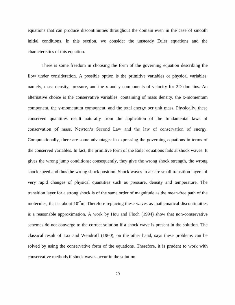
)())()((2

1),( RLRL

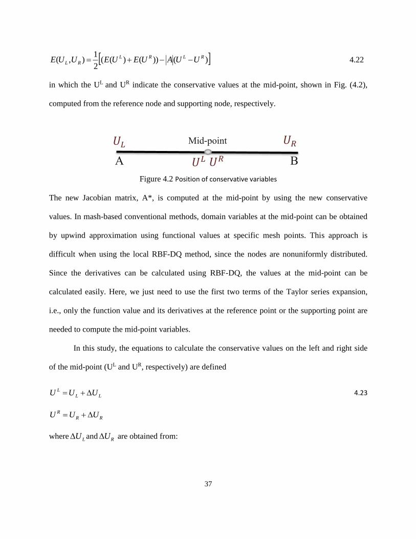
RL UUAUEUEUUE 4.22

in which the UL and UR indicate the conservative values at the mid-point, shown in Fig. (4.2),

computed from the reference node and supporting node, respectively.

Figure 4.2 Position of conservative variables

The new Jacobian matrix, A*, is computed at the mid-point by using the new conservative

values. In mash-based conventional methods, domain variables at the mid-point can be obtained

by upwind approximation using functional values at specific mesh points. This approach is

difficult when using the local RBF-DQ method, since the nodes are nonuniformly distributed.

Since the derivatives can be calculated using RBF-DQ, the values at the mid-point can be

calculated easily. Here, we just need to use the first two terms of the Taylor series expansion,

i.e., only the function value and its derivatives at the reference point or the supporting point are

needed to compute the mid-point variables.

In this study, the equations to calculate the conservative values on the left and right side

of the mid-point (UL and UR, respectively) are defined

LL

L UUU 4.23

RR

R UUU

where LU and RU are obtained from:

A B

Mid-point 𝑈𝐿 𝑈𝑅

𝑈𝐿 𝑈𝑅

38

2.

2. LRRLRR

L

yy

y

Uxx

x

UU 4.24

2.

2. RLRRLR

R

yy

y

Uxx

x

UU

To decrease the dissipation of using low shape parameters in the smooth regions, we

combine the blended method with the above formula to calculate ΔUL and ΔUR. This means that

similar formula as Eq. (4.24) are used with a high shape parameter for completely smooth

regions and two different values are saved for each of ΔUL and ΔUR . Since the higher scheme

can cause spurious numerical oscillation around discontinuities and high steep gradient regions, a

monotonic solution can not be obtained unless special treatment is enforced. Therefore, to

eliminate the presence of these oscillations, an essential principle was then suggested in the

reconstruction procedure, i.e., a ‘limiter’. In this study, after the employment of a limiter, the

variables are modified as

elseU

UUUsUUUsU

UUUsUUUsU

U

L

LkLLk

Low

L

Low

L

LkLLk

High

L

High

L

L )max()min(

)max()min(

4.25

in which the superscript High and Low refer to high and low shape parameters and subscript k

denotes all the support nodes of reference point i, and s denotes a Van Albada limiter (Sweby,

1984), which for the high shape parameter can be expressed as

22 )

2()(

)2

(**2

LRHigh

L

LRHigh

LHigh

UUU

UUU

s 4.26

39

where is a very small number (for example, e = 10-6), to prevent division by zero in a uniform

flow region, where the flux difference is very small. For the case of a low shape parameter, we

just need to substitute the low value into the equation.

Summery

To summarize this chapter we first discussed the Euler equation and then the

methodology for capturing a shock wave. The blended localized RBF-DQ includes two

approximation steps in the spatial discretization. These steps have a huge impact on the accuracy

and consistency of the algorithm. The first approximation is to calculate the conservative values

and consequently evaluate fluxes at the mid-point by using a good approximate upwinding

scheme. We then approximate the divergence of the flux field by applying a weighted linear sum

of function values at a number of discrete nodes inside the subdomain. The domain variable at

the mid-point blends into three categories based on the position of the node. The following

flowchart Fig. (4.3) illustrates the algorithm.

40

Figure 4.3 Present algorithm flowchart

41

CHAPTER 5- COMPERISSIBLE FLOW BENCHMARK

Benchmark Problem

For the case of compressible flow with the presence of a discontinuity, a supersonic

scramjet engine is simulated. Supersonic flow passes through the system, and the result is the

presence of successive oblique shocks. The computational domain is displayed in Fig. (5.1). The

sharp wedge on the top wall creates the first oblique shock, and the subsequent reflections from

the bottom wall and the wedge surface generate the reflected waves. The exact solution was

provided by Wang and Widhopf (1989) and we can clearly see in Fig. (5.7) the accurate position

of the reflections. The objective of this section is to verify the accuracy of the present meshless

method using a uniform distribution of nodes with a specific set of initial and boundary

conditions.

Problem domain

As shown in Fig. (5.1), the top wall rotates -10.94°, generating a shock structure. Some

similar, but simpler problems have been widely used as a benchmark for numerical schemes

dealing with shocks (Tota, 2006). The total number of node is 1296, distributed uniformly in the

domain as shown in Fig.(5.2) with 1177 interior nodes and 119 defining boundaries. The

number of points within a subdomain is limited to 9, including the reference node itself for all

the nodal distributions. Choosing nodes is an important issue in shock capturing problems. To

more accurately capture the discontinuities the support nodes in different direction and nodes

with the same direction along the joint line between the reference and support node were

removed. A schematic of the nodal configuration for the subdomains is shown in Fig. (5.3).

42

Figure 5.1 Benchmark domain

Figure 5.2 Node distribution

Figure 5.3 Configuration in subdomain

43

The flow variables at interior nodes are updated by the solution of Eq. (4.12) as time

marches. The treatment is different for the case of boundary nodes. It is clear that appropriate

boundary conditions are needed for the well-posed hyperbolic partial differential equation. Here,

two classes of boundary conditions are considered: solid boundary conditions; and inflow and

outflow boundary conditions.

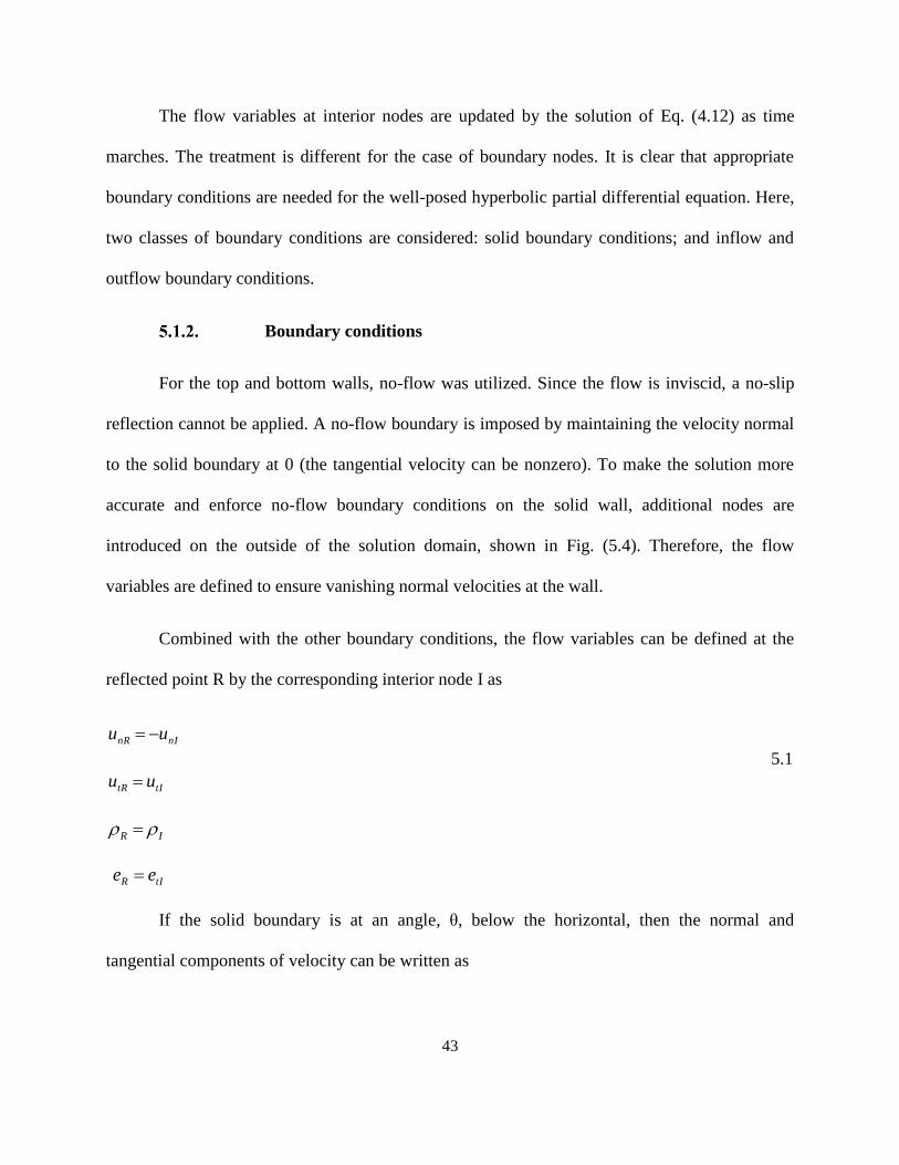
Boundary conditions

For the top and bottom walls, no-flow was utilized. Since the flow is inviscid, a no-slip

reflection cannot be applied. A no-flow boundary is imposed by maintaining the velocity normal

to the solid boundary at 0 (the tangential velocity can be nonzero). To make the solution more

accurate and enforce no-flow boundary conditions on the solid wall, additional nodes are

introduced on the outside of the solution domain, shown in Fig. (5.4). Therefore, the flow

variables are defined to ensure vanishing normal velocities at the wall.

Combined with the other boundary conditions, the flow variables can be defined at the

reflected point R by the corresponding interior node I as

nInR uu

tItR uu

5.1

IR

tIR ee

If the solid boundary is at an angle, θ, below the horizontal, then the normal and

tangential components of velocity can be written as

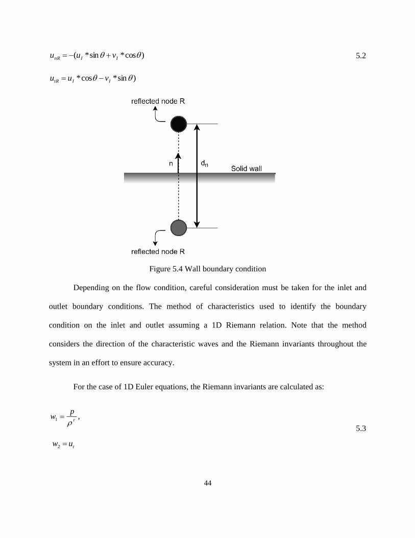
44

)cos*sin*( IInR vuu 5.2

)sin*cos* IItR vuu

Figure 5.4 Wall boundary condition

Depending on the flow condition, careful consideration must be taken for the inlet and

outlet boundary conditions. The method of characteristics used to identify the boundary

condition on the inlet and outlet assuming a 1D Riemann relation. Note that the method

considers the direction of the characteristic waves and the Riemann invariants throughout the

system in an effort to ensure accuracy.

For the case of 1D Euler equations, the Riemann invariants are calculated as:

r

pw

1 ,

tuw 2

5.3

45

)1(

23

cuw n

,

)1(

23

cuw n

where un and ut are the normal and tangential velocity components at the inlet or outlet.

Rearranging, we can obtain the primitive variables as:

2

43 wwun

,

2wut

5.4

1

1

1

2

.

w

c,

rwp .1

Following the above equations and theory of characteristic waves for supersonic flow, no

additional treatment is required. For a supersonic upstream, the domain variables are fixed from

the free stream value. For the exit condition, the values are calculated from the interior nodes.

For the current benchmark, the inlet state is supersonic and its condition specified by

prescribing the pressure, density and velocity vector as fixed. The inlet condition is the same as

the reference value (Wang & Widhopf, 1989) for the nondimensional form of governing

equation, and they are shown in Table (5.1).

Since the flow at the outlet is still supersonic, the following first-order extrapolation is

implemented,

21*2 outletoutletoutlet UUU 5.5

46

Table 5.1 Inlet condition

The computations are performed with different shape parameters and local timesteps. For

the temporal discretization in Eq. (4.12), a local timestep based of the CFL condition is used for

the explicit method. For each subdomain, a specific timestep is calculated. The size of the

subdomains was set to 9 nodes.

The results were compared with the exact solution and two conventional numerical

methods the finite volume and discontinuous Galerkin method. The results actually appear to be

better than the conventional methods in some cases.

The Mach number and pressure contours are shown in Fig (5.5) and Fig (5.6),

respectively. The method successfully captures the shock and agrees with the numerical

methods.

The finite volume model using a Steger Warming scheme Fig. (5.8) and a second order

discontinuous galerkin, Fig. (5.9), were run with a fine grid to obtain accurate results. The

number of nodes for the FV case was 9456 and for DG was 4544. Fig (5.10) shows the pressure

Pressure 0.714

Density 1.0

Mach Number 2.9

Y component of velocity 0

47

value along the bottom wall. The location of the shock agrees with the exact solution, along with

the location of the reflected wave.

Effect of parameters

Shape parameter

We also studied the effect of the shape parameter on the accuracy of the solution. A high

shape parameter increases the condition number and consequently leads to ill-conditioning of the

problem. Here we used two shape parameters to calculate the domain variables at the midpoint to

evaluate the fluxes. For incompressible flow, the values are generally high. Using a blended

scheme, we tried to increase the accuracy in the smooth region and eliminate the dissipation

caused by low value shape parameter. Using just one small shape parameter results in a low

value domain variable.

Size of subdomain

The size of the subdomain has a great impact on the results. We compared results for

different subdomains and tried to use the optimum value. The results for a subdomain of 5 was

quite inaccurate. On the other hand, a subdomain of 15 was quite good but the computation time

and cost were high. Therefore, we compromised with a subdomain of 9 nodes which gave good

result with low computation time and cost.

Slope limiter

In this study we used the Van Albada limiter (Sweby, 1984) to eliminate spurious

oscillations near shocks. By using the limiter, we could increase the order of accuracy in the

upwinding scheme and obtain higher resolution. The rate of convergence for a first order scheme

48

is faster than using a second order scheme. However, by increasing the order of the scheme with

the limiter, the residual does not drop the value like the first order and it oscillated around a

much higher value than schemes without the limiter. Therefore, if we want to avoid oscillations

near discontinuities we need to pay this unavoidable cost.

Time step

As mentioned in Chapter 4, a local time step was employed. The term local implies that

the time were determined by the means of the subdomain, i.e., within each subdomain, a specific

time step is used to calculate new domain variables. Chiu (2011) emphasizes that when one uses

a uniform time step for the whole domain in a localized meshless method, the constraint on the

time step usually depends upon the spectral radii of the inviscid flux Jacobian associated with the

solution nodes with the smallest subdomain. Here for the each subdomain the time step was

calculated by

i

ii

rCFLt

5.5

where ri is the subdomain radius and λi is the maximum wave speed. This is the time step for the

ith reference node. Therefore, different time step, based on the size of subdomain and maximum

wave speed result in saving the computation time. This method works when the limit of time

accuracy is not important anymore. For the case of final time restriction, we need to use the

global time step.

49

Postprocessing

One of the great features of meshless methods is that one can do postprocessing

separately. To show results with high resolution, we can define a new system of subdomains

with a high number of nodes inside the whole domain and/or subdomains. The procedure is

exactly the same as the processing method while in the post processing step we introduce more

nodes with just performing one iteration. Therefore the result can be interpolated on more nodes

with higher resolution.

50

Figure 5.5 Mach number contour

Figure 5.6 Pressure contour

51

Figure 5.7 Pressure contour using Finite Volume Method

Figure 5.8 Pressure contour using DG Method

52

Figure 5.9 Exact solution (Wang & Widhopf, 1989)

Figure 5.10 Pressure along the bottom wall

53

CHAPTER 6- CONCLUSION AND FUTURE WORK

Summary of work

In this study, we have presented a meshless based solver to capture shocks and

discontinuities. Nonlinear convection dominant problems can produce discontinuities, even with

a smooth initial condition. Numerical schemes need to be able to distinguish the direction of

wave propagation to capture shocks. Since there is no connectivity among the nodes in a

meshless method, the scheme must be able to identify upstream and downstream flows.

The numerical scheme used here was based on RBF-DQ to approximate the function

derivatives and an upwinding scheme added to the system to capture the shock wave

propagation. The localized RBF-DQ method is very sensitive to the shape parameter, size of the

subdomain and the number of nodes distributed within the domain.

The model was first tested using three incompressible fluid flow benchmarks i.e., the

Cavity flow problem, Natural convection, and forced convection over a backward facing step.

The result were in a good agreement with previous studies. After assuring that the scheme and

based algorithm were effective and accurate, we employed it on an Euler equation problem with

the presence of oblique shocks within the domain.

In order to increase the resolution, a second order Roe’s scheme with a Van Albada

limiter was applied to calculate the fluxes at the mid-points. The scheme was then used to

simulate the supersonic flow within a scramjet configuration and the effect of involved

parameters on the solution were examined. Results of the present scheme were compared with

54

finite volume and discontinuous Galerkin techniques, and was found to be robust and accurate in

capturing shocks location.

Future work

Meshless methods and especially RBFs, are particularly promising an alternative for

solving fluid flow. Recently many research studies have focused on the meshless method. Since

this method is more recent than other methods, there are still issues that need more investigation.

Studying the effect of the shape parameter is an important issue. This constant varies case by

case and there is no theoretical approach yet to identify the optimum value for each problem. A

bad value for the shape parameter can lead to inappropriate results. Parallel processing is the

other potential feature of the meshless method that is attractive for the future. Since the domain

is typically divided into a number of smaller subdomains, we can distribute operation among the

processors to speed up the algorithm and save the computation time. Nodes distribution

techniques is another important parameter. Here one might implement several statistical methods

to find the best way to establish node distribution based on the problem difficulties.

Adaptation techniques can also be added to the meshless method to improve accuracy.

Since mesh connectivity is no longer existent here, the process of adding or removing a node is

very comfortable and easy.

55

APPENDIX: NOMENCLATURE

A Jacobian matrix B 0; PrRaT

cShape parameter

Cvis Pr;1/Re

Ct 1;1/Pr

diThe distance between the ith data point

and its nearest neighbor

Ei Fluxes at the mid-point

E Total energy

e Internal energy

F Fluxes in x direction

g Gravity

G Fluxes in y direction

H Enthalpy

L Reference length

NI Internal node

N all collocation points in the domain

p dimensional pressure

Pe Peclet number

VLPe

Pr Prandtl number

Pr

Pj point

ri Radial dimension

Re Reynolds number

VLRe

Ra Rayleigh number

3)( LTTgRa ch

s Van Albada limiter

t Time

t̂ Dimensional time

T Temperature

T̂ Dimensional temperature

cT Cold (or reference) temperature

hT Hot temperature (heated wall)

U Conservative variables

u x component of velocity nV Velocity at nth time level *V Intermediate velocity

V̂ Dimensional velocity vector v y component of velocity

xw1 RBF-DQ for first x derivative

yw1 RBF-DQ for first y derivative

Gas constant

λi Maximum wave speed Thermal diffusivity

B Coefficient of thermal expansion

Density

Dynamic viscosity

Kinematic viscosity

Radial basis function

Entire domain

j Local domain of influence

Del operator

p Pressure gradient

t Time step

it Local time step

https://en.wikipedia.org/wiki/Thermal_diffusivity

https://en.wikipedia.org/wiki/Density

https://en.wikipedia.org/wiki/Dynamic_viscosity

https://en.wikipedia.org/wiki/Viscosity#Kinematic_viscosity

56

REFERENCES

Afiatdoust, F., & Esmaeilbeigi, M. (2015). Optimal variable shape parameters using genetic

algorithm for radial basis function approximation. Ain Shams Engineering Journal, 6(2),

639–647.

Armaly, B., Durst, F., Pereira, J., & Schonung, B. (1983). Experimental and theoretical

investigation of backward-facing step flow. Journal of Fluid Mechanics, 127, 473–496.

https://doi.org/10.1017/S0022112083002839

Atluri, S. N., & Zhu, T. (1998). A new Meshless Local Petrov-Galerkin (MLPG) approach in

computational mechanics. Computational Mechanics, 22(2), 117–127.

https://doi.org/10.1007/s004660050346

Atluri, S. N., & Zhu, T. (2000). New concepts in meshless methods. International Journal for

Numerical Methods in Engineering. https://doi.org/10.1002/(SICI)1097-

0207(20000110/30)47:1/3<537::AID-NME783>3.0.CO;2-E

Batina, J. T. (1993). A gridless Euler/Navier–Stokes solution algorithm for complex aircraft

applications. In 31st Aerospace Sciences Meeting. AIAA.

Belytschko, T., Krongauz, Y., Organ, D., Fleming, M., & Krysl, P. (1996). Meshless methods:

An overview and recent developments. Computer Methods in Applied Mechanics and

Engineering, 139(1–4), 3–47. https://doi.org/10.1016/S0045-7825(96)01078-X

Belytschko, T., Lu, Y. Y., & Gu, L. (1994). Element???free Galerkin methods. International

Journal for Numerical Methods in Engineering, 37(2), 229–256.

https://doi.org/10.1002/nme.1620370205

Chorin, A. J. (1968). Numerical Solution of the Navier-Stokes Equations. Mathematics of

Computation, 22(104), 745. https://doi.org/10.2307/2004575

Chorin, A. J., & Marsden, J. E. (1993). A Mathematical Introduction to Fluid Mechanics.

Performance Evaluation (Vol. 4). https://doi.org/10.1007/978-1-4612-0883-9

Duarte, C. A., & Oden, J. T. (1996). An h-p adaptive method using clouds. Computer Methods in

Applied Mechanics and Engineering, 139(1–4), 237–262. https://doi.org/10.1016/S0045-

7825(96)01085-7

Franke, C., & Schaback, R. (1998). Solving partial differential equations by collocation using

radial basis functions. Applied Mathematics and Computation, 93, 73–82.

https://doi.org/10.1016/S0096-3003(97)10104-7

Franke, R. (1982). Scattered data interpolation: tests of some methods. Mathematics of

Computation, 38(157), 181–181. https://doi.org/10.1090/S0025-5718-1982-0637296-4

57

Gingold, R. a., & Monaghan, J. J. (1977). Smoothed particle hydrodynamics-theory and

application to non-spherical stars. Monthly Notices of the Royal Astronomical Society, 181,

375–389. https://doi.org/10.1093/mnras/181.3.375

Godunov, S. K. (1959). A finite-difference method for the numerical computation of

discontinuous solutions of the equations of fluid dynamics. Matematicheskii Sbornik, 47,

271–306.

Hardy, R. L. (1971). Multiquadric equations of topography and other irregular surfaces. Journal

of Geophysical Research, 76(8), 1905–1915. https://doi.org/10.1029/JB076i008p01905

Harris, M., Kassab, A., & Divo, E. (2017). An Rbf Interpolation Blending Scheme For Effective

Shock-capturing. International Journal of Computational Methods and Experimental

Measurements, 5(3), 281–292.

Hou, T. Y., & Floch, P. G. Le. (1994). Why Nonconservative Schemes Converge to Wrong

Solutions: Error Analysis. Mathematics of Computation, 62(206), 497.

https://doi.org/10.2307/2153520

Kansa, E. J. (1990). Multiquadrics-A scattered data approximation scheme with applications to

computational fluid-dynamics-II solutions to parabolic, hyperbolic and elliptic partial

differential equations. Computers and Mathematics with Applications, 19(8–9), 147–161.

https://doi.org/10.1016/0898-1221(90)90271-K

Kwan Yu Chiu. (2011). A conservative meshless framework for conservation laws with

applications in computational fluid dynamics.

Larsson, E., & Fornberg, B. (2003). A numerical study of some radial basis function based

solution methods for elliptic PDEs. Computers & Mathematics with Applications, 46(5–6),

891–902. https://doi.org/10.1016/S0898-1221(03)90151-9

Lax, P., & Wendroff, B. (1960). Systems of conservation laws. Communications on Pure and

Applied Mathematics, 13(2), 217–237. https://doi.org/10.1002/cpa.3160130205

LeVeque, R. J. (1992). Numerical Methods for Conservation Laws. Mathematics of Computation

(Vol. 57). https://doi.org/10.2307/2938728

Ling, L., & Kansa, E. J. (2005). A least-squares preconditioner for radial basis functions

collocation methods. Advances in Computational Mathematics, 23(1–2), 31–54.

https://doi.org/10.1007/s10444-004-1809-5

Liszka, T. J., Duarte, C. A. M., & Tworzydlo, W. W. (1996). hp-Meshless cloud method.

Computer Methods in Applied Mechanics and Engineering, 139(1–4), 263–288.

https://doi.org/10.1016/S0045-7825(96)01086-9

Liu, G. R. (2010). Meshfree Methods: Moving Beyond the Finite Element Method. Meshfree

Methods. https://doi.org/10.1115/1.1553432

58

Liu, W. K., Jun, S., Li, S., Adee, J., & Belytschko, T. (1995). Reproducing kernel particle

methods for structural dynamics. International Journal for Numerical Methods in

Engineering, 38(10), 1655–1679. https://doi.org/10.1002/nme.1620381005

Lu, Y. Y., Belytschko, T., & Gu, L. (1994). A new implementation of the element free Galerkin

method. Computer Methods in Applied Mechanics and Engineering, 113(3–4), 397–414.

https://doi.org/10.1016/0045-7825(94)90056-6

Lucy, L. B. (1977). A numerical approach to the testing of the fission hypothesis. The

Astronomical Journal, 82, 1013. https://doi.org/10.1086/112164

Mai-Duy, N., & Tran-Cong, T. (2002). Mesh-free radial basis function network methods with

domain decomposition for approximation of functions and numerical solution of Poisson’s

equations. Engineering Analysis with Boundary Elements, 26(2), 133–156.

https://doi.org/10.1016/S0955-7997(01)00092-3

Monaghan, J. J. (1988). An introduction to SPH. Computer Physics Communications, 48(1), 89–

96. https://doi.org/10.1016/0010-4655(88)90026-4

Morinishi, K. (1995). A gridless type solution for high Reynolds number multielement flow

fields. In AIAA Paper.

Mukherjee, Y. X., & Mukherjee, S. (1997). The boundary node method for potential problems.

International Journal for Numerical Methods in Engineering, 40(June 1996), 797–815.

https://doi.org/10.1002/(SICI)1097-0207(19970315)40:5<797::AID-NME89>3.0.CO;2-#

Nayroles, B., Touzot, G., & Villon, P. (1992). Generalizing the finite element method: Diffuse

approximation and diffuse elements. Computational Mechanics, 10(5), 307–318.

https://doi.org/10.1007/BF00364252

Noguchi, H., Kawashima, T., & Miyamura, T. (2000). Element free analyses of shell and spatial

structures. International Journal for Numerical Methods in Engineering, 47(6), 1215–1240.

https://doi.org/10.1002/(SICI)1097-0207(20000228)47:6<1215::AID-NME834>3.0.CO;2-

M

Onate, E., Idelsohn, S., Zienkiewicz, O. C., Taylor, R. L., & Sacco, C. (1996). A stabilized finite

point method for analysis of fluid mechanics problems. Computer Methods in Applied

Mechanics and Engineering, 139(1–4), 315–346. https://doi.org/Doi 10.1016/S0045-

7825(96)01088-2

Randles, P. W., & Libersky, L. D. (1996). Smoothed Particle Hydrodynamics: Some recent

improvements and applications. Computer Methods in Applied Mechanics and Engineering,

139(1–4), 375–408. https://doi.org/10.1016/S0045-7825(96)01090-0

Roe, P. L. (1981). Approximate Riemann solvers, parameter vectors, and difference schemes.

Journal of computational physics. Journal of Computational Physics, 43(2), 357–372.

59

Sarler, B., & Vertnik, R. (2006). Meshfree explicit local radial basis function collocation method

for diffusion problems. Computers and Mathematics with Applications, 51(8 SPEC. ISS.),

1269–1282. https://doi.org/10.1016/j.camwa.2006.04.013

Shu, C., Ding, H., Chen, H. Q., & Wang, T. G. (2005). An upwind local RBF-DQ method for

simulation of inviscid compressible flows. Computer Methods in Applied Mechanics and

Engineering, 194(18–20), 2001–2017. https://doi.org/10.1016/j.cma.2004.07.008

Shu, C., Ding, H., & Yeo, K. . (2003). Local radial basis function-based differential quadrature

method and its application to solve two-dimensional incompressible Navier–Stokes

equations. Computer Methods in Applied Mechanics and Engineering, 192(7–8), 941–954.

https://doi.org/10.1016/S0045-7825(02)00618-7

Sweby, P. K. (1984). High Resolution Schemes Using Flux Limiters for Hyperbolic

Conservation Laws. SIAM Journal on Numerical Analysis, 21(5), 995–1011.

https://doi.org/10.1137/0721062

Temam, R. (2000). Navier-Stokes Equations: Theory and Numerical Analysis.

Tota, P. V. (2006). Meshless Euler solver using radial basis functions for solving inviscid

compressible flows.

Wang, J. C. T., & Widhopf, G. F. (1989). A high-resolution tvd finite volume scheme for the

euler equations in conservation form. Journal of Computational Physics, 84(1), 145–173.

https://doi.org/10.1016/0021-9991(89)90186-1

Wang, J. G., & Liu, G. R. (2002). On the optimal shape parameters of radial basis functions used

for 2-D meshless methods. Computer Methods in Applied Mechanics and Engineering,

191(23–24), 2611–2630. https://doi.org/10.1016/S0045-7825(01)00419-4

Waters, J., & Pepper, D. W. (2015). Global versus localized RBF meshless methods for solving

incompressible fluid flow with heat transfer. Numerical Heat Transfer, Part B:

Fundamentals, 68(3), 185–203.

Wu, Y. L. & Shu, C. (2002). Development of RBF-DQ method for derivative approximation and

its application to simulate natural convection in concentric annuli. Computational

Mechanics, 29(6), 477–485.

Yao, G., Siraj-Ul-Islam, & Sarler, B. (2012). Assessment of global and local meshless methods

based on collocation with radial basis functions for parabolic partial differential equations in

three dimensions. Engineering Analysis with Boundary Elements, 36(11).

https://doi.org/10.1016/j.enganabound.2012.04.012

Zhou, X., Hon, Y. C., & Li, J. (2003). Overlapping domain decomposition method by radial

basis functions. Applied Numerical Mathematics, 44(1–2), 241–255.

https://doi.org/10.1016/S0168-9274(02)00107-1

60

CURRICULUM VITAE

Graduate College



Degrees:

Bachelor of Science in Chemical Engineering 2014

Isfahan University of Technology

Isfahan, Iran

Thesis topic: CFD Simulation of Flow Boiling With OpenFOAM

Master of Science, Mechanical Engineering 2016


Las Vegas, Nevada

Thesis topic: Meshless Method for Simulate of Compressible Flow

Honor Membership:

Tau Beta Pi, The Engineering Society, 2016- Present

Publications: E. Nabizadeh, D. W. Pepper, “A Localized RBF-MQ Meshless Method for Simulating Compressible Flows”, American Society of Thermal and Fluids Engineers (ASTFE) Conference, April 2017 E. Nabizadeh, D. W. Pepper, and J. Waters, “Simulating Hydraulic Fracturing and Contaminant Transport with MATLAB and COMSOL Multiphysics Software”. COMSOL conference Boston, Oct. 2016 E Nabizadeh Shahrebabak, S Golafshan, MR Chamani, “Simulation of Air Flow through Skylight in Historical House, Case Study: Historic House of Mosavar-al-Molki”. International Journal of Architectural Engineering and Urban Planning, Jun. 2016 E Nabizadeh Shahrebabak, MR Chamani, S Golafshan, “Thermal Behavior of Skylight in Historical House, Case Study: Historic House of Mosavar-al-Molki”. (under review)

61

Thesis Examination Committee:

Chairperson, Dr. Darrell W. Pepper, Ph.D.

Committee Member, Dr. Hui Zhao, Ph.D.

Committee Member, Dr. William Culbreth, Ph.D.

Graduate College Faculty Representative, Dr. Laxmi Gewali, Ph.D.

meshless method for simulation of compressible flow

Documents