mercurys magnetosphere - clasp...

Advances in Space Research 33 (2004) 1859–1874

www.elsevier.com/locate/asr

Mercury�s magnetosphere

J.A. Slavin *

NASA GSFC, Laboratory for Extraterrestrial Physics, Code 696, Greenbelt, MD 20771, USA

Received 5 January 2003; received in revised form 27 February 2003; accepted 27 February 2003

Abstract

The Mariner 10 observations of Mercury�s miniature magnetosphere collected during its close encounters in 1974 and 1975 are

reviewed. Subsequent data analysis, re-interpretation and theoretical modeling, often influenced by new results obtained regarding

the Earth�s magnetosphere, have greatly expanded our impressions of the structure and dynamics of this small magnetosphere. Of

special interest are the Earth-based telescopic images of this planet�s tenuous atmosphere that show great variability on time scales of

tens of hours to days. Our understanding of the implied close linkage between the sputtering of neutrals into the atmosphere due to

solar wind and magnetospheric ions impacting the regolith and the resultant mass loading of the magnetosphere by heavy planetary

ions is quite limited due to the dearth of experimental data. However, the influence of heavy ions of planetary origin (Oþ, Naþ, Kþ,Caþ and others as yet undetected) on such basic magnetospheric processes as wave propagation, convection, and reconnection

remain to be discovered by future missions. The electrodynamic aspects of the coupling between the solar wind, magnetosphere and

planet are also very poorly known due to the limited nature of the measurements returned by Mariner 10 and our lack of experience

with a magnetosphere that is rooted in a regolith as opposed to an ionosphere. The review concludes with a brief summary of major

unsolved questions concerning this very small, yet potentially complex magnetosphere.

Published by Elsevier Ltd on behalf of COSPAR.

Keywords: Mercury’s magnetosphere; Reconnection; Substorms

1. Introduction

Owing to its magnetic field, slow rotation rate, close

proximity to the sun and lack of a dense atmosphere,

Mercury occupies a unique position in the solar-plane-tary hierarchy (Russell et al., 1988). The magnitude of its

magnetic moment is sufficiently large that it can stand-off

the solar wind above the surface under most conditions,

but it is weak to the point where Mercury occupies most

of the forward magnetosphere. The volume threaded by

magnetic flux tubes that are ‘‘closed’’ (i.e., both ends

rooted in the planet) is so small that any ‘‘trapped’’

charged particle populations are expected to be transientand associated with recent substorm activity. However,

the most significant difference between this magneto-

sphere and those of the other planets with global mag-

netic fields may be the tenuous nature of its atmosphere.

* Tel.: +1-301-286-5839; fax: +1-301-286-1648.

E-mail address: [email protected] (J.A. Slavin).

0273-1177/$30. Published by Elsevier Ltd on behalf of COSPAR.

doi:10.1016/j.asr.2003.02.019

Planetary atmospheres are important sources of ions

that may become assimilated into the magnetospheric

charged particle populations. And, in turn, these atmo-

spheres are major sinks for the energy drawn from the

solar wind by their magnetospheres. At Mercury it ap-pears that a unique situation exists where the magneto-

sphere couples directly to the regolith to create a source

for new atmospheric neutrals through sputtering while

simultaneously acting as a sink by sweeping up newly

ionized atoms. Finally, the significance of Mercury’s

unique location deep in the inner heliosphere must be

appreciated. Solar wind pressure and interplanetary

magnetic field intensity at Mercury’s perihelion are typ-ically one order of magnitude higher than is the case at

the Earth and more than two orders of magnitude

greater than at Jupiter (e.g., see Slavin and Holzer, 1981).

Launched on November 2, 1973, Mariner 10 (M10)

carried out an initial reconnaissance of the innermost

planet during its three encounters with Mercury on

March 29, 1974, September 21, 1974 and March 16,

1975. All fly-bys occurred at a heliocentric distance of

mail to: [email protected]

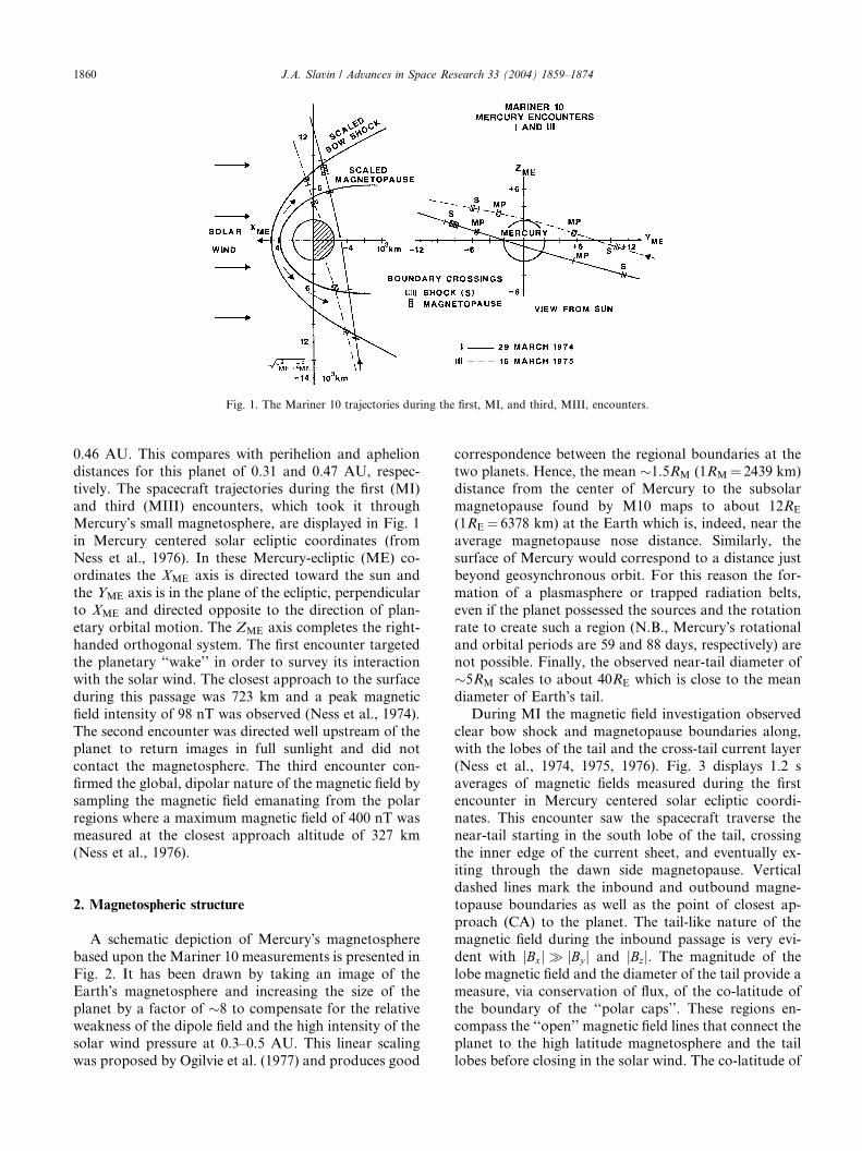
Fig. 1. The Mariner 10 trajectories during the first, MI, and third, MIII, encounters.

1860 J.A. Slavin / Advances in Space Research 33 (2004) 1859–1874

0.46 AU. This compares with perihelion and aphelion

distances for this planet of 0.31 and 0.47 AU, respec-

tively. The spacecraft trajectories during the first (MI)

and third (MIII) encounters, which took it throughMercury�s small magnetosphere, are displayed in Fig. 1

in Mercury centered solar ecliptic coordinates (from

Ness et al., 1976). In these Mercury-ecliptic (ME) co-

ordinates the XME axis is directed toward the sun and

the YME axis is in the plane of the ecliptic, perpendicular

to XME and directed opposite to the direction of plan-

etary orbital motion. The ZME axis completes the right-

handed orthogonal system. The first encounter targetedthe planetary ‘‘wake’’ in order to survey its interaction

with the solar wind. The closest approach to the surface

during this passage was 723 km and a peak magnetic

field intensity of 98 nT was observed (Ness et al., 1974).

The second encounter was directed well upstream of the

planet to return images in full sunlight and did not

contact the magnetosphere. The third encounter con-

firmed the global, dipolar nature of the magnetic field bysampling the magnetic field emanating from the polar

regions where a maximum magnetic field of 400 nT was

measured at the closest approach altitude of 327 km

(Ness et al., 1976).

2. Magnetospheric structure

A schematic depiction of Mercury�s magnetosphere

based upon the Mariner 10 measurements is presented in

Fig. 2. It has been drawn by taking an image of the

Earth�s magnetosphere and increasing the size of the

planet by a factor of �8 to compensate for the relative

weakness of the dipole field and the high intensity of the

solar wind pressure at 0.3–0.5 AU. This linear scaling

was proposed by Ogilvie et al. (1977) and produces good

correspondence between the regional boundaries at the

two planets. Hence, the mean �1.5RM (1RM ¼ 2439 km)

distance from the center of Mercury to the subsolar

magnetopause found by M10 maps to about 12RE

(1RE ¼ 6378 km) at the Earth which is, indeed, near the

average magnetopause nose distance. Similarly, the

surface of Mercury would correspond to a distance just

beyond geosynchronous orbit. For this reason the for-

mation of a plasmasphere or trapped radiation belts,

even if the planet possessed the sources and the rotation

rate to create such a region (N.B., Mercury�s rotationaland orbital periods are 59 and 88 days, respectively) arenot possible. Finally, the observed near-tail diameter of

�5RM scales to about 40RE which is close to the mean

diameter of Earth�s tail.During MI the magnetic field investigation observed

clear bow shock and magnetopause boundaries along,

with the lobes of the tail and the cross-tail current layer

(Ness et al., 1974, 1975, 1976). Fig. 3 displays 1.2 s

averages of magnetic fields measured during the firstencounter in Mercury centered solar ecliptic coordi-

nates. This encounter saw the spacecraft traverse the

near-tail starting in the south lobe of the tail, crossing

the inner edge of the current sheet, and eventually ex-

iting through the dawn side magnetopause. Vertical

dashed lines mark the inbound and outbound magne-

topause boundaries as well as the point of closest ap-

proach (CA) to the planet. The tail-like nature of themagnetic field during the inbound passage is very evi-

dent with jBxj � jBy j and jBzj. The magnitude of the

lobe magnetic field and the diameter of the tail provide a

measure, via conservation of flux, of the co-latitude of

the boundary of the ‘‘polar caps’’. These regions en-

compass the ‘‘open’’ magnetic field lines that connect the

planet to the high latitude magnetosphere and the tail

lobes before closing in the solar wind. The co-latitude of

Fig. 2. Schematic view of the bow shock and magnetosphere of Mercury.

Fig. 3. The mariner 10 magnetic field observations (1.2 s average)

taken during the first encounter.

J.A. Slavin / Advances in Space Research 33 (2004) 1859–1874 1861

the polar cap at Mercury is �25� as compared with a

value of �16� at Earth indicating that the region of

closed field lines are limited to lower latitudes than at the

Earth. The existence of such a region of closed magnetic

field lines is supported by the narrowband �2 s period

waves found by Russell (1989) in the MI magnetic field

observations. These ULF waves are very similar to those

frequently observed in the inner magnetosphere of theEarth suggesting that M10 did indeed penetrate into the

closed field line region.

The magnetic field measurements taken during MIII

encounter are displayed in Fig. 4 (from Ness et al.,

1976). The interplanetary magnetic field (IMF) was di-rected northward both before and after the encounter.

Hence, conditions were unfavorable for dayside recon-

nection and the input of energy into the magnetosphere

and very smooth magnetic profiles were observed as

shown in Fig. 4. The MII magnetic field measurements

were of critical importance because they confirmed that

the magnetosphere was indeed produced by the inter-

action of the solar wind with a global-scale magneticfield. Once corrected for the differing closest approach

distances, the polar magnetic fields measured during

MIII are about twice as large as those along the low

latitude MI trajectory. This indicates that Mercury’s

magnetic field is primarily dipolar. Although significant

uncertainties exist as to the contributions to the ob-

served field by magnetospheric current systems and to

higher order planetary magnetic fields, the magnitude ofMercury’s dipole moment is between 300 and 500 nT –

R3M with a tilt relative,to the planetary rotation axis of

about 10� (Connerney and Ness, 1988). Unfortunately,

the spatial coverage provided by MI and MIII were not

sufficient to separate out the contributions from higher

order multipoles with any confidence (Connerney and

Ness, 1988). Future progress will require not only a

more spatially complete set of measurements, but alsothe development of more comprehensive and accurate

magnetospheric current system models (Korth et al.,

2004; Giampieri and Balogh, 2001).

The plasma investigation was hampered by a

deployment failure which kept it from returning any ion

Fig. 4. Mariner 10 magnetic field observations made during the third fly-by on March 16, 1975.


measurements. Fortunately, the electron portion of the

plasma instrument did work as planned (Ogilvie et al.,

1974). For both passes good correspondence was found

between the magnetic field and plasma measurements as

to the locations of the bow shock and magnetopause

boundaries. Furthermore, plasma speed and density

parameters derived from the electron data producedconsistent results regarding bow shock jump conditions

and pressure balance across the magnetopause (Slavin

and Holzer, 1979; Ogilvie et al., 1977). Within Mercury�smagnetosphere, plasma density was found to be higher

than that observed at Earth by a factor comparable to

the ratio of the external solar wind density at the orbits

of the two planets (Ogilvie et al., 1977). Throughout the

MI pass plasma sheet-type distributions were observedwith an increase in temperature beginning near closest

approach coincident with the energetic particle events.

In contrast, the MIII took the spacecraft through

the high latitude magnetosphere where it observed the

‘‘horns’’ of a cool, quite-time plasma sheet (Ogilvie

et al., 1977; Ness et al., 1976).

3. Magnetospheric dynamics

The M10 observations have left the impression that

Mercury�s magnetosphere may be amongst the most

dynamic in the solar system. Whether or not this is true

cannot be verified until more comprehensive, longer

duration measurements are returned by the MESSEN-

GER and BepiColombo, Missions (Solomon et al.,

2001; Grard and Balogh, 2001). Following the same 8

to 1 scaling as used earlier, Fig. 5 displays same of the

dynamic features that may be present at Mercury duringmagnetospheric substorm according to the near-earth

neutral line (NENL) theory of substorms (Slavin et al.,

2002; Baker et al., 1996). The reconnection x-line that

typically forms �)20 to )30RE behind the Earth would

be expected to lie at about )3RM at Mercury. This near-

Mercury neutral line (NMNL) is the site where lobe

magnetic field energy is dissipated to power high-speed

plasma flow, plasma heating, and energetic particle ac-celeration. As shown in Fig. 5, ‘‘jets’’ of plasma emanate

from the x-line with speeds comparable to the Alfven

speed in the flux tubes undergoing reconnection. These

flows are usually very time dependent with the sunward

and anti-sunward flows in the terrestrial magnetosphere

being termed ‘‘bursty bulk flows’’ (Angelopoulos et al.,

1992) and ‘‘post-plasmoid plasma sheet flows’’ (Rich-

ardson et al., 1987), respectively. The anti-sunwardflows slow as they compress the dipolar magnetic fields

closer to the planet and create a high pressure region

that is thought to drive strong field-aligned currents into

and out of the ionosphere called the ‘‘substorm current

Fig. 5. A schematic view of the substorm expansion phase at Mercury based upon the NENL model.


wedge’’, or SCW (Shiokawa et al., 1998). This slowing

is most pronounced in the Earth�s magnetosphere atdowntail distances of X�)16 to )12RE (Baumjohann

et al., 1990) which should correspond to )2 to )1.5RM

at Mercury. These high-speed flows often contain mag-

netic flux ropes or loop-like structures that have di-

mensions of a few Earth radii in the near-tail, but grow

to have diameters of �10RE or more in the distant

downstream tail (Slavin et al., 1999; Ieda et al., 1998).

An example of such a large tailward moving structure,called a plasmoid or plasmoid-rype flux rope, in Mer-

cury�s tail is depicted in Fig. 5 (in yellow). By the stan-

dard scaling rule, these plasmoids would be expected to

grow to several Mercury radii in diameter.

Turning to the dayside interaction, the mean distance

from the center of Mercury to the subsolar magneto-

pause based upon the M10 observations is about 1.5RM

(Russell, 1977; Ness et al., 1976). Slavin and Holzer(1979) further found that the subsolar distances ex-

trapolated from the individual magnetopause and bow

shock crossings, after scaling for upstream ram pressure

effects, varied from 1.3 to 2.1RM with the larger values

corresponding to IMF Bz > 0 and the smaller to Bz < 0.

They attributed this variability to the transfer, or ‘‘ero-

sion’’, of magnetic flux from the dayside magnetosphere

into the tail. Whether or not the solar wind is ever ableto compress and/or erode the dayside magnetosphere to

the point where solar wind ions could directly impact the

surface at low latitudes remains a topic of considerable

interest and controversy. Siscoe and Chirstopher (1975)

were the first to take a long time series of solar wind rampressure data taken at 1 AU, scale it by 1/r2 inward to

Mercury�s perihelion, and then compute the solar wind

stand-off distance using various assumed planetary

magnetic moments. They found that only a few percent

of the time will the magnetopause be expected to fall

below an altitude of �0.1RM or the point where solar

wind protons will begin to strike the surface due to finite

gyro-radius effects. Shorter lived, large amplitude in-creases in solar wind ram pressure associated with high-

speed streams and interplanetary shocks might be

expected to easily depress the magnetopause close to the

surface of planet. However, theoretical models have

shown that induction currents should be readily gener-

ated in the planetary interior to resist such rapid com-

pressions (Glassmeier, 2000; Hood and Schubert, 1979).

Moreover, model calculations by Suess and Goldstein(1979) have indicated that the magnetic flux added to

the dayside magnetosphere by these induction currents

becomes especially important as the magnetopause is

compressed below �0.2RM. In fact, their model predicts

that the ram pressure increase required to drive the

magnetopause to 0.1RM may be an order of magnitude

more than what would be required in the absence of

induction effects.Magnetopause erosion is a well-known consequence

of magnetic reconnection between the IMF and plane-

tary magnetic fields and reduces the distance to the


subsolar magnetopause at the Earth by �1–2RE for a

typical interval of southward IMF (Sibeck et al., 1991).

The most direct evidence that reconnection operates at

Mercury�s magnetopause takes the form of ‘‘flux trans-

fer events’’ identified in the M10 data by Russell and

Walker (1985). These discrete, flux rope-like structuresare a well accepted signature of reconnection at the

terrestrial magnetopause. Approximately �10–20% of

the southward IMF impinging upon the dayside mag-

netopause at the Earth undergoes this reconnection (see

Slavin and Holzer, 1979) and is pulled back into the

magnetotail. In the terrestrial magnetosphere excess

magnetic flux in tail may be stored for tens of minutes to

a few hours before rapid reconnection in the cross-tailcurrent layer returns it to the dayside. The possibility

exists that Mercury may lack the ability to store excess

magnetic flux in its tail due to the effective absence of an

electrically conducting ionosphere. Luhmann et al.

(1998) have suggested, for example, that flux addition to

the tail will rapidly lead to the reconnection of a like

amount of flux in the tail. This would eliminate the

‘‘growth phase’’ of terrestrial substorms during whichenergy is stored in the tail prior to expansion phase

onset (McPherron et al., 1973). However, even assuming

Luhmann�s hypothesis is correct, there would still be

some minimal convection time delays in the magneto-

sheath and then the tail as the magnetic flux is trans-

ported to and from the dayside magnetosphere. Such a

minimum convective ‘‘response time’’ was estimated by

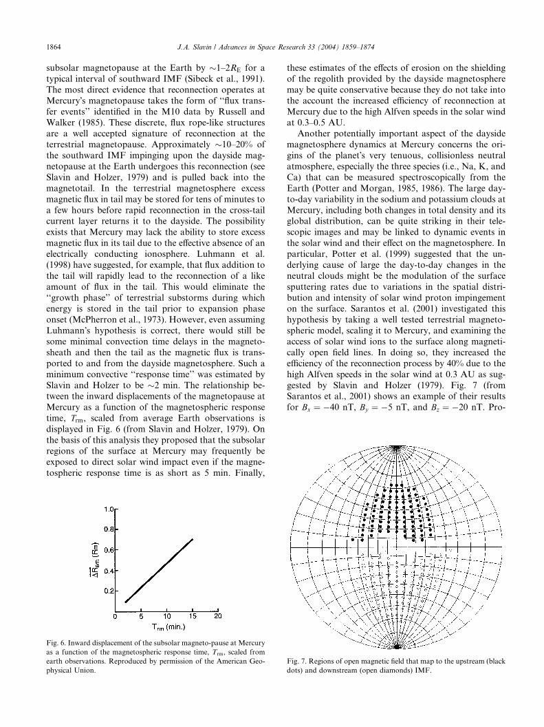
Slavin and Holzer to be �2 min. The relationship be-tween the inward displacements of the magnetopause at

Mercury as a function of the magnetospheric response

time, Trm, scaled from average Earth observations is

displayed in Fig. 6 (from Slavin and Holzer, 1979). On

the basis of this analysis they proposed that the subsolar

regions of the surface at Mercury may frequently be

exposed to direct solar wind impact even if the magne-

tospheric response time is as short as 5 min. Finally,

Fig. 6. Inward displacement of the subsolar magneto-pause at Mercury

as a function of the magnetospheric response time, Trm, scaled from

earth observations. Reproduced by permission of the American Geo-

physical Union.

these estimates of the effects of erosion on the shielding

of the regolith provided by the dayside magnetosphere

may be quite conservative because they do not take into

the account the increased efficiency of reconnection at

Mercury due to the high Alfven speeds in the solar wind

at 0.3–0.5 AU.Another potentially important aspect of the dayside

magnetosphere dynamics at Mercury concerns the ori-

gins of the planet�s very tenuous, collisionless neutral

atmosphere, especially the three species (i.e., Na, K, and

Ca) that can be measured spectroscopically from the

Earth (Potter and Morgan, 1985, 1986). The large day-

to-day variability in the sodium and potassium clouds at

Mercury, including both changes in total density and itsglobal distribution, can be quite striking in their tele-

scopic images and may be linked to dynamic events in

the solar wind and their effect on the magnetosphere. In

particular, Potter et al. (1999) suggested that the un-

derlying cause of large the day-to-day changes in the

neutral clouds might be the modulation of the surface

sputtering rates due to variations in the spatial distri-

bution and intensity of solar wind proton impingementon the surface. Sarantos et al. (2001) investigated this

hypothesis by taking a well tested terrestrial magneto-

spheric model, scaling it to Mercury, and examining the

access of solar wind ions to the surface along magneti-

cally open field lines. In doing so, they increased the

efficiency of the reconnection process by 40% due to the

high Alfven speeds in the solar wind at 0.3 AU as sug-

gested by Slavin and Holzer (1979). Fig. 7 (fromSarantos et al., 2001) shows an example of their results

for Bx ¼ �40 nT, By ¼ �5 nT, and Bz ¼ �20 nT. Pro-

Fig. 7. Regions of open magnetic field that map to the upstream (black

dots) and downstream (open diamonds) IMF.

Fig. 8. MHD simulation of the magnetosphere of Mercury revealing

flux tube topology via color coding; tan field lines are interplanetary,

magenta field lines are closed, and white and blue field lines are open.


jected down upon the dayside hemisphere are the foot

prints of recently ‘‘opened’’ field lines that connect the

planetary surface to the solar wind. The empty region at

low latitudes corresponds to the small portion of the

surface still shielded from the solar wind by closed

magnetic field lines. The new feature uncovered is thestrong asymmetry introduced by the very strong IMF Bx

field component which results in the field lines emanat-

ing from the northern/southern hemispheres mapping to

the upstream/downstream solar wind for negative/posi-

tive IMF Bx, respectively. Hence, the black dots and

open diamonds in Fig. 7 both correspond to newly

opened field lines, but only the northern hemisphere

(i.e., black dots) connects to the upstream solar wind(for strongly negative Bx) and channels solar wind

protons to the surface where sputtering may produce an

enhanced outward flux of neutral atoms. Interplanetary

sector crossings, for example, are a common source of

reversals in the polarity of IMF Bx and could contribute

to the neutral atmospheric variability observed by Potter

et al. (1999) over Mercury�s poles by means of the

hemispheric asymmetries predict by Sarantos et al.(2001).

Recently, a similar analysis has been carried out by

Leblanc et al. (2003) for solar energetic particles (i.e.,

ions with energies >10 keV/amu) accelerated in associ-

ation with coronal mass ejections. They also found that

charged particle access to the surface of Mercury de-

pended critically upon the IMF and that the fluxes of

sputtered neutrals resulting from such surface impactscould be highly asymmetric and represent a possible

explanation for Potter et al.’s variable neutral cloud

distribution.

Many of the features found in the analytical models

of Mercury�s magnetosphere are reproduced in the new

global MHD and hybrid simulations of the solar wind

interaction with this planet (Kallio and Janhunen, 2003;

Ip and Kopp, 2002; Kabin et al., 2000). For example, asshown in Fig. 8 (from Kabin et al., 2000), the region of

closed magnetic fields extended no farther poleward

than �50� latitude in good agreement with the analytical

models. The magnetic fields emanating from the polar

regions do indeed map back into the lobes of the tail,

but with the strong north/north asymmetry in the

draping of the newly opened flux tubes that was also

found by Sarantos et al. (2001). In Fig. 8 the recentlyopened blue field lines that connect to the upstream

solar wind and allow direct impact of solar wind ions on

the surface while the white field lines only map to the

downstream solar wind. Global MHD simulations by Ip

and Kopp (2002) and hybrid simulations by Kallio and

Janhunen (2002) produced qualitatively similar results,

especially respect to the strong effects of IMF Bz and Bx

on the magnetic topology of the dayside magnetosphereand its affect on interplanetary charged particle access to

the surface.

A substorm is a magnetosphere-wide disturbance that

channels large amounts of electromagnetic energy, ei-

ther drawn directly from the solar wind or first stored in

the tail lobes, into plasma sheet heating, high speed bulk

plasma flows, energetic particle acceleration, and field-

aligned currents. In addition to producing large scale

reconfiguration of the tail magnetic fields and high speedplasma flow, the magnetic and electric field changes

during substorms act together to ‘‘inject’’ energetic

particles into the inner magnetosphere where they drift

about the Earth until lost due to charge exchange,

scattering into the loss cone, or ‘‘shadowing’’ of the drift

path by the magnetopause. Furthermore, the rapid

B-field changes at x-lines produce large inductive electric

fields that populate the ‘‘separatrix layers’’ between thex-line and the slow shocks that mark the outermost re-

connected field lines with accelerated particles (Cowley,

1980). Observationally, spacecraft often observe ener-

getic ions and electrons with energies of tens of keV to

several Mev in the deep tail during substorms (Rich-

ardson et al., 1996; Sarris and Axford, 1979). On the

sunward side of the x-line these charged particles will be

further energized as they convected toward the planetand conserve their first adiabatic invariant. Hence, a

particle transported from the Earth�s central plasma

sheet to the ring current region could experience a factor

of 103 or 104 increase in energy as the magnetic field

intensity grows by a similar amount. At Mercury, by

comparison, this type of ‘‘betatron’’ acceleration may

raise the energy of the ‘‘seed’’ particles by only a factor

of �102 due to the relative weakness of the magneticfields external to the planet.

As reported by Simpson et al. (1974), four separate,

several minute long enhancements were recorded which

they termed the A, B (and B0), C and D events. The

nature of the particles being measured has been the


subject of some controversy because of instrumental

effects associated with the extremely high count rates

(Eraker and Simpson, 1986). However, the most likely

source would appear to be electrons with energies

greater than 35 keV (Christon, 1987). Each of the events

is characterized by rapid rises followed by several min-ute long decays back to the background levels; albeit

this behavior is least well defined for the relatively weak

‘‘A’’ event. All of the energetic particle events observed

by M10 occurred during the outbound leg of MI when

very disturbed magnetic fields were observed. Finally, it

should be noted that the C event straddled the outbound

magnetopause crossing while the D event was observed

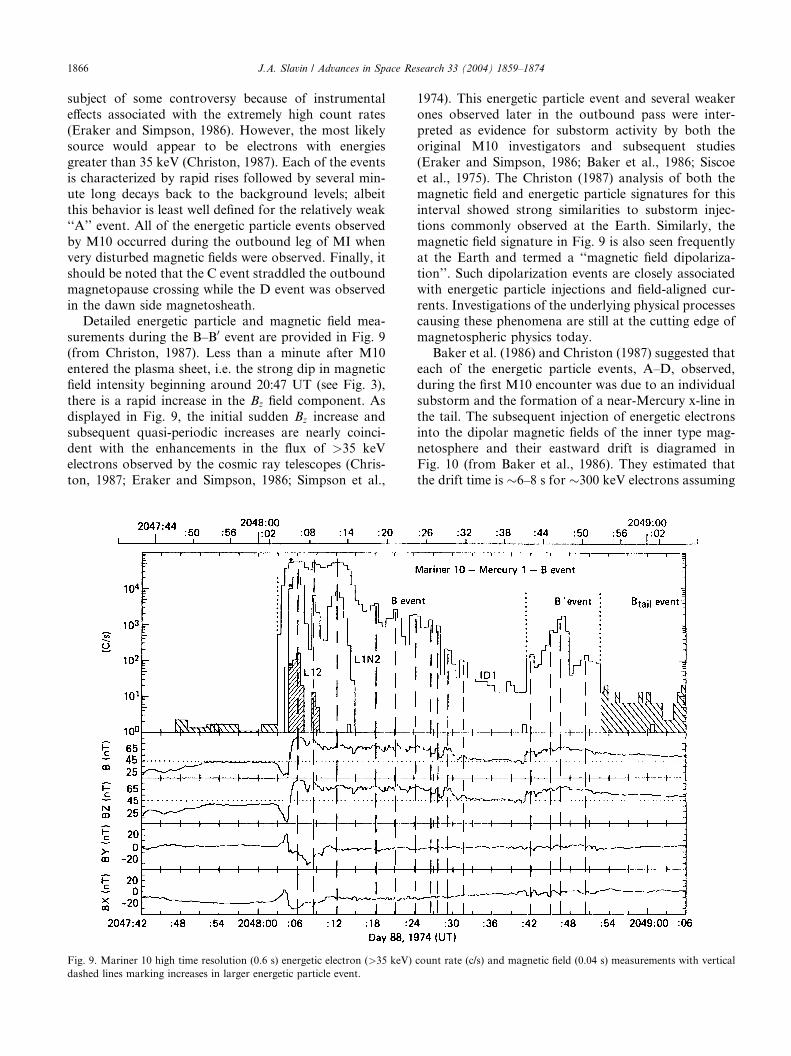
in the dawn side magnetosheath.Detailed energetic particle and magnetic field mea-

surements during the B–B0 event are provided in Fig. 9

(from Christon, 1987). Less than a minute after M10

entered the plasma sheet, i.e. the strong dip in magnetic

field intensity beginning around 20:47 UT (see Fig. 3),

there is a rapid increase in the Bz field component. As

displayed in Fig. 9, the initial sudden Bz increase and

subsequent quasi-periodic increases are nearly coinci-dent with the enhancements in the flux of >35 keV

electrons observed by the cosmic ray telescopes (Chris-

ton, 1987; Eraker and Simpson, 1986; Simpson et al.,

Fig. 9. Mariner 10 high time resolution (0.6 s) energetic electron (>35 keV)

dashed lines marking increases in larger energetic particle event.

1974). This energetic particle event and several weaker

ones observed later in the outbound pass were inter-

preted as evidence for substorm activity by both the

original M10 investigators and subsequent studies

(Eraker and Simpson, 1986; Baker et al., 1986; Siscoe

et al., 1975). The Christon (1987) analysis of both themagnetic field and energetic particle signatures for this

interval showed strong similarities to substorm injec-

tions commonly observed at the Earth. Similarly, the

magnetic field signature in Fig. 9 is also seen frequently

at the Earth and termed a ‘‘magnetic field dipolariza-

tion’’. Such dipolarization events are closely associated

with energetic particle injections and field-aligned cur-

rents. Investigations of the underlying physical processescausing these phenomena are still at the cutting edge of

magnetospheric physics today.

Baker et al. (1986) and Christon (1987) suggested that

each of the energetic particle events, A–D, observed,

during the first M10 encounter was due to an individual

substorm and the formation of a near-Mercury x-line in

the tail. The subsequent injection of energetic electrons

into the dipolar magnetic fields of the inner type mag-netosphere and their eastward drift is diagramed in

Fig. 10 (from Baker et al., 1986). They estimated that

the drift time is �6–8 s for �300 keV electrons assuming

count rate (c/s) and magnetic field (0.04 s) measurements with vertical

Fig. 10. Schematic view of energetic particle acceleration at a near-

Mercury neutral line and subsequent ‘‘injection’’ into the inner mag-

netosphere. Reproduced by permission of the American Geophysical

Union.


a closed path. The C and D events at the dawn mag-

netopause and in the magnetosheath were attributed to

electrons being injected onto drift paths intersecting the

dawn-side magnetopause. No energetic particle events

were detected during the MIII high latitude encounter(Eraker and Simpson, 1986) presumably due to the

northward IMF and lack of substorm activity at the

time of that encounter.

Although not measured by M10, the drift trajectories

for energetic ions in Mercury�s small magnetosphere

have been the subject of extensive modeling. In partic-

ular, Lukyanov et al. (2001) investigated the fate of

energetic protons originating in a 1RM wide source re-gion at the anticipated distance of the near-Mercury

neutral line, �2–3RM downstream of the planet. For

energies 6 10 keV the ExB drift dominates the gradient

and curvature drifts and the protons intercept the sur-

face of Mercury near midnight. As the energy increases

to 30–50 keV, the curvature and gradient drifts become

more important and a partial ring forms about the

planet with many ions hitting the planet on the daysideor escaping through the dawn-side magnetopause.

Above 50 keV nearly all of the protons encounter the

planetary surface or the magnetopause within a few

seconds.

4. Electrodynamic coupling

Magnetospheres are tightly coupled to their planets

by field-aligned currents (FACs) that flow along the

magnetic lines of force linking the two. Any stress ex-

erted upon the planetary magnetic field by the external

solar wind or internal dynamics, such as reconnection

and convection, generates field aligned currents. They

may exist either as steady-state currents or as pulses of

current carried by Alfven waves. These FACs self-con-

sistently alter the magnetospheric magnetic field until a

new equilibrium is reached. In the terrestrial case, the

scale for changes in these currents systems is quite brief,

tens of seconds to a few minutes, because the Alfven

speed, VA, is very high; i.e., of order 103 km/s every-where outside of the plasma sheet. Based upon the M10

plasma and magnetic field results, similar speeds might

be expected within the high latitude Hermean magne-

tosphere. For example, based upon the MIII encounter

measurements in the high latitude magnetosphere typi-

cal values of B� 50 nT and np � 1 cm�3 would appear to

be representative with an implied Alfven speed of

VA ¼ B=ffiffiffi

4p

pnpmp � 1000 km/s. However, if heavy ionssuch as Oþ or Naþ are the dominate ion species, then

the Alfven speed would be reduced and the ‘‘bounce

times’’ increased as much as a factor of �6. Still, as

pointed out by Glassmeier (1997) and Luhmann et al.

(1998), the transit time from a NMNL at X�)3RM to

the surface of the planet at the lower latitude edge of the

polar cap would be only �10 s and the multiple reflec-

tions to reach equilibrium would take only �1 min.Three principal FAC systems are commonly observed

at the Earth. The ‘‘Region 1’’ currents are driven by the

solar wind interaction with the geomagnetic field at the

magnetopause and its boundary layers. The ‘‘Region 2’’

currents are driven by plasma pressure gradients in the

inner magnetosphere. And, third, the ‘‘substorm current

wedge’’ currents in the midnight local time sector are

generated by the pressure gradients generated in thenear-tail by the braking of earthward directed high-

speed flows out of the NENL. The sense of both the

Region 1 and SCW systems is downward toward the

planet on the dawn-side and outward on the dusk-side.

Fig. 11 depicts the locations of these current systems at

Mercury assuming that they are able to close near the

surface by some as yet unknown mechanism. The Re-

gion 2 currents are not shown because the pressuregradients that drive them map to below the surface of

Mercury according to the familiar 8 to 1 spatial scaling

relation. Finally, Fig. 11 displays a portion of the in-

duction currents that may be driven in the planetary

interior by solar wind pressure variations (Glassmeier,

2000; Suess and Goldstein, 1979). The sense of these

induction currents is to oppose rapid changes in the pre-

existing magnetic field configuration so that the stress towhich the B-field is responding is opposed.

In the early-1970s, it was thought that both Mercury

and Mars might possess small intrinsic field magneto-

spheres. Although Mars Global Surveyor measurements

(Acuna et al., 1998) have now shown that this is not the

case for Mars, the possibility of twin small magneto-

spheres, one with no ionosphere (Mercury) and one with

an ionosphere (Mars) more highly conducting than thatof the Earth, spawned new ideas regarding the role of

electrical conductance of the region at the foot of

Fig. 11. Schematic view of the electrodynamic interaction between the magnetosphere and Mercury mediated by field aligned currents (green) and

induction currents (orange).


magnetospheric flux tubes. Coroniti and Kennel (1973)

argued that ionospheric conductivity will act as a‘‘brake’’ or ‘‘regulator’’ on the rate of convection within

magnetospheres. This effect, usually referred to as ‘‘line-

tying’’, occurs because ionospheric plasma, convecting

in response to the electric field imposed by the magne-

tosphere, experiences a net drag force as a result of

collisions with atmospheric neutral species. These colli-

sions allow ionospheric ions and electrons some motion

parallel to the direction of the electricfield, as opposed tothe ExB drift direction. In doing, they so generate Pe-

derson conductivity that enables Joule dissipation. The

greater the ionospheric Pederson conductivity is the

larger the power that must be drawn from the solar wind

to maintain a given electric potential across the polar

cap. The lower the electrical conductivity in the polar

cap is the closer the potential drop across the magne-

tosphere will approach to the maximum voltage appliedby the solar wind, USW. Such effects have now been re-

produced by global simulations (see Fedder and Lyon,

1987).

The electric potential applied to the magnetosphere is

the product of the solar wind flow speed in the mag-

netosheath times the normal magnetic field component

to the magnetopause integrated about the circumference

of the tail lobes. However, it can be approximated by theproduct of the upstream solar wind speed, the compo-

nent of the IMF opposite to the planetary magnetic field

at the dayside magnetopause and the length of the x-lineat the dayside magnetopause (assumed to be compara-

ble to the solar wind stand-off distance). Hence, given

typical solar wind parameters at 1 AU, e.g., 400 km/s

with an embedded southward IMF of magnitude 3 nT

and a 10RE width for the dayside x-line, the external

USW applied to the Earth�s magnetosphere would be 77

kV. However, it should be noted during an encounter

with a magnetic cloud embedded in a coronal massejection the Earth�s magnetosphere might experience a

500 km/s solar wind with southward IMF of 10 nT

which corresponds to an applied electric potential of 320

kV. For Mercury at perihelion, the mean IMF intensity

should be about a factor of 9 greater than that experi-

enced at the Earth due to the 1/r2 gradient with distance

from the sun. Accordingly, at Mercury perihelion typi-

cal solar wind conditions of 400 km/s and a southwardIMF of )27 nT and an assumed day-side x-line width of

�1.5RM will result in the application of an electric po-

tential of �40 kV to the Hermean magnetosphere. For

more extreme conditions corresponding to 500 km/s and

)90 nT, the potential drop applied to the magnetosphere

could reach 165 kV.

Rassbach et al. (1974) and Hill et al. (1976) built

upon these concepts and further proposed that iono-spheric conductivity may in turn affect the cross polar

Fig. 12. Four minutes of M10 magnetic field measurements centered

on the field-aligned current event identified.


cap potential, Upc, by limiting the rate at which recon-

nection opens field lines at the dayside magnetopause.

They argued that if ionospheric conductivity becomes

high enough for the electric current closing across the

planetary polar cap to generate significant magnetic

fields at the magnetopause, then the reconnection pro-cess could be disrupted. In this manner Rassbach and

Hill argued that ionospheric Pedersen conductance, R,limits the cross polar cap electric potential drop ac-

cording to the relationship Upc 6Usw=ð1þ R=R0Þ whereR0 � 20 mho. At the Earth, the nightside ionosphere has

a conductance of only a few mhos away from auroral

arcs, but the dayside conductance can exceed 10 mho.

Hence, the cross polar cap potential tends to ‘‘saturate’’as it approaches Upc ¼ 2=3ðUswÞ. For this reason values

over �150–200 kV are seldom observed regardless of the

potential applied by the solar wind (see Siscoe et al.,

2002).

Based upon the available atmospheric models (Hun-

ten et al., 1988), the height integrated conductance of

Mercury’s nearly collisionless ionosphere has been esti-

mated to be only � 5 � 10�6 mho (Lammer and Bauer,1997). Surface conductance is a strong function of

composition and mineralogy, but the value of 0.1 mho

suggested by Hill et al. (1976) is not unreasonable. Al-

ternative scenarios for generating electrical conduc-

tance, such as the pickup of newly created exospheric

ions (Cheng et al., 1987) or photoelectron sheaths

(Grard and Balogh, 2001; Grard et al., 1999) have not

identified mechanisms for producing height integratedconductances greater than �1 mho. Under these con-

ditions, the electric potential drop across Mercury’s

polar cap and magnetosphere should be set by the solar

wind with Upc � Usw. Hence, at perihelion the typical

electric potential drop across this small magnetosphere

will typically reach a few tens of kilovolts with the

average value at aphelion being less by a factor of �2.

Another expectation based upon the anticipated poorelectrical conductivity of Mercury’s tenuous ionosphere

and regolith is that the field aligned currents linking the

magnetosphere and ionosphere may dissipate very rap-

idly as they quickly give up their energy to Joule heating

in the highly resistive regolith. For these reasons, the

strong variations in the east-west component of the

magnetospheric magnetic field, By, measured by M10

between 20:50:55 to 20:51:18 during the first encounter,and displayed in Fig. 12 (from Slavin et al., 1997), came

as a surprise. This bipolar variation in the DBy � 60 nT,

was the largest perturbation in this component of the

field recorded during either MI or MIII (also see Figs. 3

and 11). This magnetic signature is well known from

measurements made by spacecraft traversing field-

aligned current sheets in the Earth’s magnetosphere

(Iijima and Potemra, 1978). At the time of the M10FAC encounter it was located at ()0.95RM, )1.56RM,

0.23RM). The corresponding distance from the center of

the planet was 1.84RM and the local time �03:50. The

average Bz around this event was about twice the mag-

nitude of Bx as would be expected for a pass though the

near-tail of the Earth at distance approaching geosyn-chronous orbit. Given the M10 trajectory (see Fig. 1),

the gradient in By between the dashed lines is consistent

with an upward FAC at the spacecraft. This upward

current sheet is largely balanced by two smaller down-

ward current sheets just before and after the central

current sheet. Indeed, multiple current sheets are very

common on the nightside of the auroral oval during.

substorms (Iijima and Potemra, 1978).Given the strong central current sheet directed into

the planet�s northern auroral zone at a point well east of

midnight, Slavin et al. (1997) suggested the M10 FACs

might be associated with the Region 1 currents which

flow into the poleward edge of the auroral zone in the

dawn hemisphere. Alternatively, it was also thought that

they might be the eastern leg of the substorm current

wedge that produced the magnetic field dipolarizationencountered earlier around 20:48 (McPherron et al.,

1973). This latter interpretation is of interest because of

the substorm energetic particle injection observed a

couple of minutes earlier. Under the assumption that the

observed magnetic field perturbation is caused by a

semi-infinite current sheet, the implied current density is

�50 mA/m. If this current sheet were indeed quasi-

aligned with a constant L-shell, then the average currentintensity in the central current sheet would be approxi-

mately 0.7 lA/m2. Both the sheet current intensity and

current density inferred in this manner from the M10

observations lie within the range of values observed in

the terrestrial magnetosphere (e.g., Iijima and Potemra,

1978). Although the current in the auroral oval at the

Earth generally varies as a function of local time, solar

wind, and substorm conditions, Slavin et al. estimated

Fig. 13. Re-circulation of sodium sputtered from the surface, photo-

ionized and carried back to the surface by magnetospheric convection.


the total current flowing into the auroral oval might be

on this occasion to be 1.4� 106 A. Again, this value lies

within the 1–3� 106 A range typically reported for the

Region 1 currents at the Earth (Iijima and Potemra,

1978). However, these FAC observations must close and

that raises the issue of the conductivity at low altitudesand the physical process(es) that support it.

The very short duration of the M10 substorm signa-

tures, about 1–2 min, as compared with �1 h at the

Earth is also intertwined with the electrodynamics of the

solar wind–magnetosphere–regolith system. Siscoe et al.

(1975) argued that substorm duration is determined by

the time necessary for plasma to convect across the

polar cap or, equivalently, from the outer boundary ofthe tail down to the mid-plane where reconnection can

take place. Using typical solar wind and magnetotail

parameters, they showed that the �1 h time scale for the

terrestrial magnetosphere could be recovered. For

Mercury the small dimensions of the magnetosphere and

the intense inter-planetary �V � B electric fields in the

inner heliosphere result in a much shorter rapid mag-

netic flux cycle time than that found in the tail of theEarth. The value calculated by Siscoe et al. was ap-

proximately 1 min, in good agreement with the duration

of the energetic particle events.

Given these short time scales for magnetic flux cycling

and the lack of terrestrial-style ionospheric line tying,

Luhmann et al. (1998) suggested that substorms at

Mercury may be largely ‘‘driven’’ by the solar wind. The

terrestrial magnetosphere often stores magnetic flux forsome variable amount time in the tail lobes before the

system becomes unstable and NENL formation takes

place. However, at other times it appears that the

magnetosphere dissipates the energy drawn from the

solar wind in a fashion that follows the inferred dayside

reconnection rate in linear manner, but with a fixed

phase lag (e.g., see Bargatze et al., 1985). These latter

substorms are classifield as being of the ‘‘driven’’ asopposed to ‘‘triggered’’ or ‘‘spontaneous’’. The deter-

mination of how substorms within these two magneto-

spheres differ is an important objective for future

missions to Mercury.

Experience with other magnetospheres, especially

Jupiter’s, has shown the important electrodynamic ef-

fects of mass loading from planetary atmospheres and

natural satellites. In the case of Mercury, Ip (1987) hassuggested that there may be a strong tendency for ions

to be ‘‘re-circulated’’ between the regolith and magne-

tosphere due to the large volume occupied by the planet

and the dominance of finite gyro-radius effects in a

magnetosphere of such small physical dimensions.

Fig. 13 (from Ip, 1987) shows how the effects of ion

impact sputtering, aided by solar radiation pressure, will

result in the injection and acceleration of newly createdions followed by further re-circulation, if they impact

and are implanted in the surface. The effects of these

heavy ions on Mercury’s magnetosphere are far from

clear, but the pickup process itself is known to create a

net electrical current that might contribute to FAC

closure at low altitudes. Cheng et al. (1987) estimated

that the magnitude of such a ‘‘pickup conductance’’ at

Mercury could reach �0.3 mho, but this number is

highly uncertain. Similarly, Glassmeier (1997) calculatedthat the Alfven conductance associated with MHD wave

propagation could increase to �1 mho if heavy ions

were sufficiently plentiful. This is important because, as

pointed out by Glassmeier, the SCW current system that

appears to operate at Mercury based upon the M10

dipolarization and FAC observations would be very

difficult to establish if the Alfven conductance were too

low. More detailed studies of ion pickup and accelera-tion are now being carried out in order to understand

the similarities and differences between such processes at

Mercury and the Earth (e.g., see Delcourt et al., 2002),

but a definitive estimate of the effect of heavy ions on

the electrodynamics of Mercury’s magnetosphere will

require new measurements.

Killen et al. (2001, 2004) found that Mercury’s at-

mosphere is sufficiently tenuous that it would soon bedepleted by losses associated with photo-ionization

and charge exchange, if it were not being continuously

replenished (see Goldstein et al., 1981). These sources

and sinks are depicted in Fig. 14 (from Killen et al.,

2001) where the state of Mercury’s atmosphere at any

given moment corresponds to the integrated effect of all

these mechanisms with significant change believed to

occur on relatively short time scales of tens of hours toa few days. Consistent with the simulations of ion

convection by Lukyanov et al. (2001), trajectory anal-

yses conducted by Killen et al. (2004) indicate that

perhaps 60% of these photo-ions may subsequently

impact the surface, where they are adsorbed and be-

come available for release via sputtering or impact va-

porization. Furthermore, if reconnection at the dayside

Fig. 14. Sources and sinks for Mercury�s tenuous atmosphere.

Reproduced by permission of the American Geophysical Union.


magnetopause frequently exposes significant fractions

of the surface directly to impact by charged particles inthe interplanetar medium, then the contribution of

neutrals sputtered off by solar wind ions (Sarantos

et al., 2001) and solar energetic particles (Leblanc et al.,

2003) to the atmosphere may be a major driver for this

system. In any event, the relatively short times required

for photo-ionization, charge exchange and electron

impact ionization will lead to sputtered neutrals being

quickly ionized and picked-up by the convective flowwithin the magnetosphere producing a closely coupled

system.

5. Summary

The Mariner 10 magnetic field measurements have

shown that Mercury has a largely dipolar magnetic fieldtilted only slightly relative to the planetary spin axis.

The interaction of this magnetic field with the solar wind

creates a miniature magnetosphere that typically stands-

off the solar wind at an altitude of �0.5RM above the

sub-solar point. Both MHD and hybrid numerical

simulations of the solar wind interaction with Mercury

support the terrestrial-type magnetosphere interpreta-

tion of the Mariner 10 observations. Hence, whencombined with knowledge gained at the Earth and from

exploring the other planetary systems, it appears that

the �30 min of measurements taken by M10 were

probably sufficient to determine the gross structure of

this magnetosphere. However, it will not be until

observations taken over an extended period of time,

including perihelion passages, become available that thefull range of structural variations can be known

including its response to extreme solar wind conditions

such as high speed streams and coronal mass ejections.

The internal dynamics of this miniature magneto-

sphere are, of course, more poorly understood. Esti-

mates of the fraction of time that the magnetopause is

sufficiently close to the planet to allow direct solar wind

impact on the surface vary from a few per cent to severaltens of per cent depending upon the assumed efficiency

of magnetic reconnection and the strength of induction

currents. The atmospheric neutral and magnetospheric

charged particle populations may be closely coupled. A

major source of neutrals is believed to be sputtering

from the regolith due to solar wind ion, solar energetic

particle and magnetospheric ion impact. And, in turn,

the ionization of atmospheric neutrals is likely to be animportant source of magnetospheric ions. The degree to

which heavy ions of planetary origin, e.g., Oþ, Naþ, Kþ,Mgþ, etc., affect magnetospheric processes is a critical

question that will be answered only with new measure-

ments. Clear evidence of substorm activity was obtained

during the second half of the first encounter in the form

of an intense magnetic field dipolarization event and

several energetic particle injections in the near-tail. Tothe extent that ion energy exceeds �50 keV, they will

generally be lost to surface impact or exit through the

dayside magnetopause on time scales of 1–10 s. For this

reason Mercury�s magnetosphere may be ideal for in-

vestigations of deep tail charged particle acceleration

because essentially all particles above certain energy can

be assumed to have undergone such acceleration within

seconds of their detection. With its compliment of amagnetometer, an energetic charged particle spectrom-

eter, a plasma analyzer with composition capability, and

a ultraviolet imager (Solomon et al., 2001), the MES-

SENGER Mission appears well-suited to studying the

dynamics of the magnetosphere during substorms and

the exchange of mass between the magnetosphere, at-

mosphere and regolith.

The other unique aspect of Mercury�s magnetosphereis its electrodynamic coupling to the solar wind above

and the planet below. The brief, several minute duration

of the substorm-like events observed by Mariner 10 has

generally been attributed to the absence of an electrically

conducting ionosphere and the resultant lack of line

tying effects. Under these conditions it might be ex-

pected that the field-aligned currents driven by internal

and external MHD stresses would be short lived and,therefore, rarely seen in spacecraft observations. It was

therefore surprising, and perhaps very fortuitous, that


Mariner 10 observed both a magnetic dipolarization

event and intense field-aligned currents during the out-

bound MI encounter. Detailed electric and magnetic

field measurements of FACs at Mercury, whether car-

ried by Alfven waves or steady-state currents closing

somehow at low altitudes, will be critical to achieving afull understanding of how this planet interacts with its

magnetosphere. Despite the small dimensions of Mer-

cury�s magnetosphere, the strong interplanetary mag-

netic fields in the inner heliosphere and its lack of a

conductive ionosphere should result in electric potential

drops of some 10�s of kV. The rapid convection driven

by these relatively large dawn-to-dusk electric fields and

the small dimensions of Mercury�s magnetosphere areconsistent with very brief substorm time scales observed

by Mariner 10. For these reasons, the BepiColombo

Mission with a low altitude planetary mapper and a high

altitude magnetospheric orbiter carrying rather com-

prehensive magnetic and electric fields and charged and

neutral particle instrumentation are well equipped to

reveal the electrodynamic aspects of this magnetospheric

system (Grard and Balogh, 2001; Blomberg, 1997).In closing, we list just a few of most important science

questions relating to Mercury�s magnetosphere:

6. Solar wind–magnetosphere interaction

• How does the rate of magnetopause reconnection at

Mercury�s orbit differ from that at the Earth? Whatis the effect on solar wind stand-off distance? On the

rate of energy transfer to the magnetosphere?

• How and where does the solar wind enter the magne-

tosphere?

• What effect does the very small IMF Parker spiral an-

gle at Mercury have on the solar wind interaction and

the magnetosphere?

• How often and where does the solar wind impact theplanet?

7. Magnetosphere–planetary coupling

• What is the electric potential drop across the magne-

tosphere?

• What is the role of FACs in magnetosphere–plane-tary coupling at Mercury? How do field-aligned cur-

rents close?

• What effect do planetary induction currents exert on

the system?

• What contributions do thermalized planetary ions

make to the magnetospheric populations? How do

they affect magnetospheric dynamics?

• Where, when, and how does reconnection take placein the tail? How does it differ from that observed at

the Earth?

• How are substorms at Mercury different from those

at Earth?

8. Charged particle acceleration

• What are the sources of Mercury’s energetic particle

populations? Planetary ion pick-up? Betatron? X-line

acceleration?• What roles do finite gyro-radius effects play in

charged particle acceleration, transport, and equilib-

rium populations? Wave-particle interactions and dif-

fusion?

• How do charged particle injections at Mercury differ

from those at Earth?

Acknowledgements

We thank all of the people who contributed to the

great success for the Mariner 10 mission especially thePrincipal Investigators for the magnetic field (N. Ness),

plasma (H. Bridge) and cosmic ray (J. Simpson) inves-

tigations. Conversations with J. Gjerloev and E. Tans-

kanen on magnetosphere-ionosphere coupling are also

gratefully acknowledged as are the very helpful sugges-

tions made by both referees.

References

Acuna, M.H. et al. Magnetic field and plasma observations at Mars:

initial results from the Mars Global Surveyor mission. Science 279,

1676–1680, 1998.

Angelopoulos, V., Baumjohann, W., Kennel, C.F., et al. Bursty bulk

flows in the inner central plasma sheet. J. Geophys. Res. 97, 4027–

4039, 1992.

Baker, D.N., Simpson, J.A., Eraker, J.H. A model of impulsive

acceleration and transport of energetic particles in Mercury’s

magnetosphere. J. Geophys. Res. 91, 8742–8748, 1986.

Baker, D.N., Pulkkinen, T.I., Angelopoulos, V., Baumjohann, W.,

McPherron, R.L. Neutral line model of substorms: past results and

present view. J. Geophys. Res. 101, 12975–13010, 1996.

Bargatze, L.F., Baker, D.N., McPherron, R.L., Hones Jr., E.W.

Magnetospheric impulse response for many levels of geomagnetic

activity. J. Geophys. Res. 90, 6387–6394, 1985.

Baumjohann, W., Paschmann, G., Luhr, H. Characteristics of high

speed ion flows in the plasma sheet. J. Geophys. Res. 95, 3801–

3809, 1990.

Blomberg, L.G. Mercury’s magnetosphere, exosphere and surface:

low-frequency field and wave measurements as a diagnostic tool.

Planet. Space Sci. 45, 143–148, 1997.

Cheng, A.F., Johnson, R.E., Krimigis, S.M., Lanzerotti, L.J. Magne-

tosphere, exosphere and surface of Mercury. Icarus 71, 430–440,

1987.

Christon, S.P. A comparison of the Mercury and Earth magneto-

spheres: electron measurements and substorm time scales. Icarus

71, 448–471, 1987.

Connerney, J.E.P., Ness, N.F. The magnetosphere of Mercury, in:

Chapman, C. (Ed.), Mercury. University of Arizona Press, pp.

494–513, 1988.


Coroniti, F.V., Kennel, C.F. Can the ionosphere regulate magneto-

spheric convection? J. Geophys. Res. 78, 2837–2851, 1973.

Cowley, S.W.H. Plasma populations in a simple open model magne-

tosphere. Space Sci. Rev. 25, 217–275, 1980.

Delcourt, D.C., Moore, T.E., Orsini, S., Millilo, A., Sauvaud, J.-A.

Centrifugal acceleration of ions near Mercury. Geophys. Res. Lett.

29 (12), 2002, doi:10.1029/2001GL013829.

Eraker, J.H., Simpson, J.A. Acceleration of charged particles in

Mercury’s magnetosphere. J. Geophys. Res. 91, 9973–9993, 1986.

Fedder, J.A., Lyon, J.G. The solar wind–magnetosphere–ionosphere

current–voltage relationship. Geophys. Res. Lett. 14, 880–883,

1987.

Giampieri, G., Balogh, A. Modeling of magnetic field measurements at

Mercury. Planet. Space Sci. 49, 1637–1642, 2001.

Glassmeier, K.-H. The Hermean magnetosphere and its I–M coupling.

Planet. Space Sci. 45, 119–125, 1997.

Glassmeier, K.-H. Currents in Mercury’s Magnetosphere, Magneto-

spheric Current Systems. AGU, Washington, DC, 2000, pp. 371–

380.

Goldstein, B.E., Suess, S.T., Walker, R.J. Mercury: magnetospheric

processes and the atmospheric supply and loss rates. J. Geophys.

Res. 86, 5485–5499, 1981.

Grard, R., Balogh, A. Return to Mercury: science and mission

objectives. Planet. Space Sci. 49, 1395–1407, 2001.

Grard, R., Laakso, H., Pulkkinen, T.I. The role of photoemission in

the coupling of the Mercury surface and magnetosphere. Planet.

Space Sci. 47, 1459–1463, 1999.

Hill, T.W., Dessler, A.J., Wolf, R.A. Mercury and Mars: the role of

ionospheric conductivity in the acceleration of magnetospheric

particles. Geophys. Res. Lett. 3, 429–432, 1976.

Hood, L.L., Schubert, G. Inhibition of solar wind impingement on

Mercury by planetary induction currents. J. Geophys. Res. 84,

2641–2647, 1979.

Hunten, D.M., Morgan, T.H., Schemansky, D.E. The Mercury

atmosphere, in: Chapman, C. (Ed.), Mercury. University of

Arizona Press, Tucson, pp. 562–612, 1988.

Ieda, A., Machida, S., Mukai, T., Saito, Y., Yamamoto, T., Nishida,

A., Terasawa, T., Kokubun, S. Statistical: analysis of plasmoid

evolution with GEOTAI observations. J. Geophys. Res. 103, 4453–

4465, 1998.

Iijima, T., Potemra, T.A. Large-scale characteristics of field-aligned

currents associated with substorms. J. Geophys. Res. 83, 599–615,

1978.

Ip, W.-H. Dynamics of electrons and heavy ions in Mercury’s

magnetosphere. Icarus 71, 441–447, 1987.

Ip, W.-H., Kopp, A. MHD simulation of the solar wind interaction

with Mercury. J. Geophys. Res. 107 (A11), 1348, 2002, doi:10.1029/

2001JA009171.

Kabin, K., Gombosi, T.I., et al. Interaction of Mercury with the solar

wind. Icarus 84, 397–406, 2000.

Kallio, E., Janhunen, J.P. Modeling the solar wind interaction with

Mercury by a quasi-neutral hybrid model. Ann. Geophys. 21 (11),

2133–2145, 2003.

Killen, R.M., Potter, A.E., Reiff, P., et al. Evidence for space weather

at Mercury. J. Geophys. Res. 106, 20509–20525, 2001.

Killen, R.M., Sarantos, M., Reiff, P. Space weather at Mercury. Adv.

Space Res., 2004 (doi:10.1016/j.asr.2003.02.020).

Korth, H., Anderson, B.J., McNutt, R.L., Jr., et al., Determination of

the properties of Mercury’s magnetic field by the MESSENGER

mission. Planet. Space Sci., 2004 (in press).

Lammer, H., Bauer, S.J. Mercury’s exosphere: origin of surface

sputtering and implications. Planet. Space Sci. 45, 73–79, 1997.

Leblanc, F., Luhmann, J.G., Johnson, R.E., Lui, M. Solar energetic

particle event at Mercury. Planet. Space Sci. 51, 339–352, 2003.

Luhmann, J.G., Russell, C.T., Tsyganenko, N.A. Disturbances in

Mercury’s magnetosphere: are the Mariner 10 ‘‘substorms’’ simply

driven. J. Geophys. Res. 103, 9113–9119, 1998.

Lukyanov, A.V., Barabash, S., Lundin, R., son Brandt, P.C. Energetic

neutral atom imaging of Mercury’s magnetosphere: 2. Distribution

of energetic charged particles in a compact magnetosphere. Planet.

Space Sci. 49, 1677–1684, 2001.

McPherron, R.L., Russell, C.T., Aubry, M.P. Satellite studies of

magnetospheric substorms on August 15, 1968, 9. Phenomenolog-

ical model for substorms. J. Geophys. Res. 78, 3131–3149,

1973.

Ness, N.F., Behannon, K.W., Lepping, R.P., et al. Observations of

magnetic field near Mercury: preliminary results from Mariner 10.

Science 185, 151–159, 1974.

Ness, N.F., Behannon, K.W., et al. Magnetic field of Mercury. J.

Geophys. Res. 80, 2708–2716, 1975.

Ness, N.F., Behannon, K.W., et al. Observations of Mercury’s

magnetic field. Icarus 28, 479–488, 1976.

Ogilvie, K.W., Scudder, J.D., Hartle, R.E., et al. Observations at

Mercury encounter by the plasma science instrument on Mariner

10. Science 185, 145–150, 1974.

Ogilvie, K.W., Scudder, J.D., Vasyliunas, V.M., Hartle, R.E., Siscoe,

G.L. Observations at the planet Mercury by the plasma electron

instrument: Mariner 10. J.Geophys. Res. 82, 1807–1824, 1977.

Potter, A.E., Morgan, T.H. Discovery of sodium in the atmosphere of

Mercury. Science 229, 651–653, 1985.

Potter, A.E., Morgan, T.H. Potassium in the atmosphere of Mercury.

Icarus 67, 336–340, 1986.

Potter, A.E., Killen, R.M., Morgan, T.H. Rapid changes in the

atmosphere of Mercury. Planet. Space Sci. 47, 1441–1448,

1999.

Rassbach, M.E., Wolf, R.A., Daniell Jr., R.E. Convection in a

Martian magnetosphere. J. Geophys. Res. 79, 1125–11127,

1974.

Richardson, I.G., Cowley, S.W.H., Hones Jr., E.W., Bame, S.J.

Plasmoid-associated energetic ion bursts in the deep geomagnetic

tail: properties of plasmoids and the post-plasmoid plasma sheet. J.

Geophys. Res. 92, 9997–10013, 1987.

Richardson, I.G., Owen, C.J., Slavin, J.A. Energetic (>0.2 MeV)

electron bursts in the deep geomagnetic tail observed by the

Goddard space flight center experiment on ISEE-3: association

with geomagnetic substorms. J. Geophys. Res. 101, 2723–2740,

1996.

Russell, C.T. On the relative locations of the bow shocks of the

terrestrial planets. Geophys. Res. Lett. 4, 387–390, 1977.

Russell, C.T., Walker, R.J. Flux transfer events at Mercury. J.

Geophys. Res. 90, 11067–11074, 1985.

Russell, C.T., Baker, D.N., Slavin, J.A. The magnetosphere of

Mercury, in: Chapman, C. (Ed.), Mercury. University of Arizona

Press, Tucson, pp. 514–561, 1988.

Russell, C.T. ULF waves in the Mercury magnetosphete. Geophys.

Res. Lett. 16, 1253–1256, 1989.

Sarantos, M., Reiff, P.H., Hill, T.W., Killen, R.M., Urquhart, A.L. A

Bx-interconnected magnetosphere model for Mercury. Planet.

Space Sci. 49, 1629–1635, 2001.

Sarris, E.T., Axford, W.I. Energetic protons near the plasma sheet

boundary. Nature 77, 460–462, 1979.

Shiokawa, K., Baumjohann, W., Haerendel, G., et al. High-speed ion

flow, substorm current wedge formation and multiple Pi2 pulsa-

tions. J. Geophys. Res. 103, 4491–4507, 1998.

Sibeck, D.G., Lopez, R.E., Roelof, B.C. Solar wind control of

magnetopause shape, location and motion. J. Geophys. Res. 96,

5489–5495, 1991.

Simpson, J.A., Eraker, J.H., Lamport, J.E., Walpole, P.H. Electrons

and protons accelerated in Mercury’s magnetosphere. Science 185,

160–166, 1974.

Siscoe, G.L., Christopher, L. Variations in the solar wind stand-off

distance at Mercury. Geophys. Res. Lett. 2, 158–160, 1975.

Siscoe, G.L., Ness, N.F., Yeates, C.M. Substorms on Mercury? J.

Geophys. Res. 80, 4359–4363, 1975.

http://dx.doi.org/10.1029/2001GL013829

http://dx.doi.org/10.1029/2001JA009171

http://dx.doi.org/10.1029/2001JA009171

http://dx.doi.org/doi:10.1016/j.asr.2003.02.020


Siscoe, G.L. et al. Hill model of transpolar potential saturation:

comparisons with MHD models. J. Geophys. Res. 107 (A6), 2002,

doi: 10.1029/2001JA000109.

Slavin, J.A., Holzer, R.E. The effect of erosion on the solar wind stand-

off distance at Mercury. J. Geophys. Res. 84, 2076–2082,

1979.

Slavin, J.A., Holzer, R.E. Solar wind flow about the terrestrial planets,

1. Modeling bow shock position and shape. J. Geophys. Res. 86,

11401–11418, 1981.

Slavin, J.A., Owen, C.J., J.Connerney, E.P., Christon, S.P. Mariner 10

observations of field-aligned currents at Mercury. Planet. Space

Sci. 45, 133–141, 1997.

Slavin, J.A. et al. Dual spacecraft observations of lobe magnetic field

perturbations before, during and after plasmoid release. Geophys.

Res. Lett. 26, 2897–2900, 1999.

Slavin, J.A., Fairfield, D.H., Lepping, R.P., et al. Simultaneous

observations of earthward flow bursts and plasmoid ejection during

magnetospheric substorms. J. Geophys. Res. 107 (A7), 2002,

doi:10.1029/2000JA003501.

Solomon, S.C. et al. The MESSENGER mission to Mercury, scientific

objectives and implementation. Planet. Space Sci. 49, 1445–1465,

2001.

Suess, S.T., Goldstein, B.E. Compression of the Hermaean magneto-

sphere by the solar wind. J. Geophys. Res. 84, 3306–3312, 1979.

http://dx.doi.org/10.1029/2001JA000109

http://dx.doi.org/10.1029/2000JA003501

mercurys magnetosphere - clasp...

Documents