memory constrained data locality optimization for tensor contractions* alina bibireata, sandhya...

Memory Constrained Data Locality Optimization for

Tensor Contractions*

Alina Bibireata, Sandhya Krishnan, Gerald Baumgartner, Daniel Cociorva, Chi-Chung Lam, P. Sadayappan, J. Ramanujam, David E. Bernholdt,

Venkatesh Choppella

*Supported by NSF and DOE

The “Tensor Contraction Engine” Addresses Programming Challenges

• User describes computational problem (tensor contractions expressions) in a simple, high-level language– Similar to what might be written

in papers

• Synthesis tool translates high-level language into traditional Fortran (or C, or…) code

• Generated code is compiled and linked to quantum chemistry suite, e.g. NWChem or GAMESS

• Productivity– User writes simple, high-level

code– Code generation tools do the

tedious work• Complexity

– Significantly reduces complexity visible to programmer

• Performance– Perform optimizations prior to

code generation– Automate many decisions

humans make empirically– Tailor generated code to target

computer – Tailor generated code to

specific problem

TCE Components

• Algebraic Transformations– Minimize operation count

• Memory Minimization– Reduce intermediate storage

• Space-Time Transformation– Trade-offs btw storage and

recomputation

• Storage Management and Data Locality Optimization– Optimize use of storage

hierarchy

• Data Distribution and Partitioning– Optimize parallel layout

Tensor Expressions

Algebraic Transformations

Memory Minimization

Performance Model

System Memory

Specification

Software Developer

Data Distribution and Partitioning

Parallel CodeFortran/C/…

OpenMP/MPI/Global Arrays

Sequence of Matrix ProductsElement-wise Matrix Operations

Element-wise Function Eval.

Space-Time Trade-Offs

Storage and Data Locality Management

No sol’n fits disk Sol’n fits disk, not mem. Sol’n fits mem.

Sol’n fits mem.

No sol’n fits disk

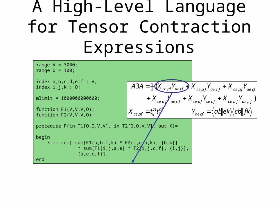
A High-Level Language for Tensor Contraction Expressions

range V = 3000;range O = 100;

index a,b,c,d,e,f : V;index i,j,k : O;

mlimit = 1000000000000;

function F1(V,V,V,O);function F2(V,V,V,O);

procedure P(in T1[O,O,V,V], in T2[O,O,V,V], out X)=

begin X == sum[ sum[F1(a,b,f,k) * F2(c,e,b,k), {b,k}]

* sum[T1[i,j,a,e] * T2[i,j,c,f], {i,j}], {a,e,c,f}];

end

fkcbekabYttX

YXYXYX

YXYXYXAA

cfaeafij

ceijafce

fceafaecfceafaecfcaefaec

cfeafaecfceafaeccfaeafce

,,

,,,,,,

,,,,,,21

)

(3

Problem Addressed in this Paper

Fus

ion

Str

uctu

re

Tile Sizes

Disk I/O

Placem

ent

Given an operation-minimal set of tensor contractions, apply loop fusion and tiling, and insert disk I/O stmts to minimize data movement cost

Current TCE prototype uses a simpler “decoupled approach”; we now develop a more integrated approach

Decoupled Approach

Explore fusion structure space first to find a memory-minimal solution

Explore tile size space and use a greedy placement of disk I/O stmts at outermost possible point in the code.

Select the solution with minimum disk access cost

Integrated Approach

Optimal Algorithm: The {fusion structure x disk placements} search

space can be decoupled from tile size space Pruning search to eliminate all inferior {fusion x

placements} solutions with respect to memory cost and disk access volume, irrespective of tile sizes

Explore the tile size space for un-pruned solutions Heuristic Algorithm:

Use memory space & disk access costs for case of unit tile size to prune more aggressively in first step

Example

k l

ljxClkBxkiA )],(),([),(

A Two Contraction example:

Ni = 3500

Nj = 3600

Nk= 3800

Nl = 4000Double Precision Arrays

Memory Limit: 10 MB

Loop Fusion

T(*,*) = 0.0FOR j, k, l T(j,k) += B(k,l) * C(j,l)D(*,*) = 0.0FOR i, j, k D(i,j) += A(i,k) * T(j,k)

Unfused Code:

D(*,*) = 0.0FOR j, k T = 0.0 FOR l T += C(j,l) * B(k,l) FOR i D(i,j) += A(i,k) * T

Fused Code after Memory Minimization

Intermediate T is reduced to a scalar, thus reducing space requirements

Disk I/O Placements



Disk I/O Placement I (For only First Contraction)

FOR j, k T = 0.0 FOR l Cm = Read C(j,l) Bm = Read B(k,l) T += Cm * Bm

Disk Access Volume

Memory Cost

C Nj x Nl x Nk 1 (for Cm)

B Nk x Nl x Nj 1 (for Bm)

Disk I/O Placements



FOR j Cm(l) = Read C(j,l) FOR k T = 0.0 Bm(l) = Read B(k,l) FOR l T += Cm(l) * Bm(l)

Disk I/O Placement II (For only First Contraction)

Disk Access Volume Memory Cost

C Nj x Nl Nl (for Cm)

B Nk x Nl x Nj Nl (for Bm)

Loop Tiling

Disk Access Volume

Memory Cost

C Nj x Nl Nl (for Cm)

B Nk x Nl x Nj Nl (for Bm)

After Loop Tiling

FOR jT

Cm(jI,l) = Read C(j,l) FOR kT

FOR jI, kI T(jI,kI) = 0.0 Bm(kI,l) = Read B(k,l) FOR lT, jI, kI, lI

T(jI,kI) += Cm(jI,lT+lI) * Bm(kI,lT+lI)

FOR j Cm(l) = Read C(j,l) FOR k T = 0.0 Bm(l) = Read B(k,l) FOR l T += Cm(l) * Bm(l)

Fused Code with I/O Placements

Disk Access Volume

Memory Cost

C Nj x Nl Nl x Tj (for Cm)

B Nk x Nl x Nj/Tj Nl x Tk (for Bm)

Decoupled Approach

Step One: Memory Minimization Finds a fusion structure that is memory minimal

Step Two: Loop Tiling and Disk I/O Placement Tiles the loops Determines tile sizes and disk I/O placements to

minimize disk access cost under memory limit constraints

Decoupled Approach

Step One: Memory Minimization


Memory minimal solution

for j

for k

for l for i

T += C(j,l) * B(k,l) D(i,j) += A(i,k) * T

Fused Code Parse Tree

Decoupled Approach

Step Two: Loop Tiling and Disk I/O Placementsfor jT

for kT

for jI

for kI

for lI

for jI

for kI

for iI

T(jI,kI) += C(jT+jI,lT+lI) * B(kT+kI,lT+lI)

D(iT+iI,jT+jI) += A(iT+iI,kT+kI) *

T(jI,kI)

Tile Sizes Found

Ti = 500 Tj = 900 Tk = 543 Tl = 500

for iT

No. of Accesses at lT: 47 MB TjTk + TjNl + TkNl

No. of Accesses at iT: 42 MB NiTj + NiTk + TjTk

Memory Limit: 10 MB

for lT

Decoupled Approach

Step Three: Loop Tiling and Disk I/O Placementsfor jT

for kT

for jI

for kI

for lI

for jI

for kI

for iI

T(jI,kI) += C(jI,lI) * B(kI,lI)

D(iI,jI) += A(iI,kI) * T(jI,kI)

for lT

Read C(jI,lI)

Read B(kI,lI)

Read D(iI,jI)

Read A(iI,kI)

Write D(iI,jI)

Disk Access Cost: 234 secs Memory Usage: 9.23 MB

Redundancy for I/O statement

for iT

Integrated Approach

Step One: Memory Minimization and Disk I/O Placement Finds a set of fusion structures with disk I/O

placements

Step Two: Loop Tiling Tiles the loops Determines tile sizes to minimize disk access cost

under memory limit constraints

Integrated Approach

Step One: Memory Minimization and Disk I/O Placementfor j

T(k) += C * B

D += A * T(k)

Read C

Read B Read A

Write D

for l for i

for k for k

Best Loop Structure with Disk I/O Placements found by Step One

Redundancy for I/O statement

No Redundancy for I/O statement

Integrated Approach

Disk Access Cost: 194 secs Memory Usage: 9.99 MB

Step Two: Loop Tiling

Tile Sizes Found

Ti = 300 Tj = 254 Tk = 308 Tl = 292

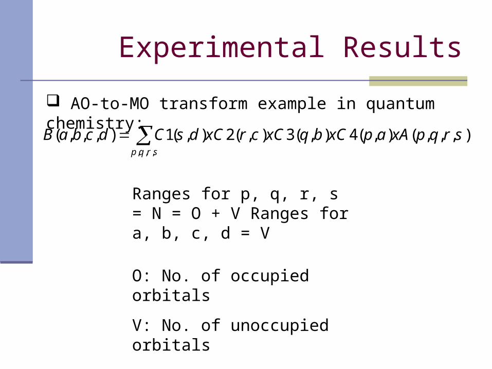
Experimental Results

srqp

srqpxAapxCbqxCcrxCdsCdcbaB,,,

),,,(),(4),(3),(2),(1),,,(

AO-to-MO transform example in quantum chemistry:

Ranges for p, q, r, s = N = O + V Ranges for a, b, c, d = V

O: No. of occupied orbitals

V: No. of unoccupied orbitals

Disk Access Costs for Both Approaches

Ranges Decoupled Integrated Improvement factor

Memory Limit = 100 MB

V=70, N=80 189 sec 80 sec 2.36

V=200, N=300 7.39 x 104 sec 1.01 x 104 sec 7.34

V=500, N=600 5.52 x 106 sec 2.33 x 105 sec 23.73


V=70, N=80 39.5 sec 39.5 sec 1.00

V=200, N=300 4.82 x 104 sec 1.004 x 104 sec 4.80

V=500, N=600 3.36 x 106 sec 2.3 x 105 sec 14.57


V=70, N=80 39.5 sec 39.5 sec 1.00

V=200, N=300 2.93 x 104 sec 1.004 x 104 sec 2.92

V=500, N=600 2.14 x 106 sec 2.3 x 105 sec 9.32

CCSD Doubles Equationhbar[a,b,i,j] == sum[f[b,c]*t[i,j,a,c],{c}] -sum[f[k,c]*t[k,b]*t[i,j,a,c],{k,c}] +sum[f[a,c]*t[i,j,c,b],{c}] -sum[f[k,c]*t[k,a]*t[i,j,c,b],{k,c}] -

sum[f[k,j]*t[i,k,a,b],{k}] -sum[f[k,c]*t[j,c]*t[i,k,a,b],{k,c}] -sum[f[k,i]*t[j,k,b,a],{k}] -sum[f[k,c]*t[i,c]*t[j,k,b,a],{k,c}] +sum[t[i,c]*t[j,d]*v[a,b,c,d],{c,d}] +sum[t[i,j,c,d]*v[a,b,c,d],{c,d}] +sum[t[j,c]*v[a,b,i,c],{c}] -sum[t[k,b]*v[a,k,i,j],{k}] +sum[t[i,c]*v[b,a,j,c],{c}] -sum[t[k,a]*v[b,k,j,i],{k}] -sum[t[k,d]*t[i,j,c,b]*v[k,a,c,d],{k,c,d}] -sum[t[i,c]*t[j,k,b,d]*v[k,a,c,d],{k,c,d}] -sum[t[j,c]*t[k,b]*v[k,a,c,i],{k,c}] +2*sum[t[j,k,b,c]*v[k,a,c,i],{k,c}] -sum[t[j,k,c,b]*v[k,a,c,i],{k,c}] -sum[t[i,c]*t[j,d]*t[k,b]*v[k,a,d,c],{k,c,d}] +2*sum[t[k,d]*t[i,j,c,b]*v[k,a,d,c],{k,c,d}] -sum[t[k,b]*t[i,j,c,d]*v[k,a,d,c],{k,c,d}] -sum[t[j,d]*t[i,k,c,b]*v[k,a,d,c],{k,c,d}] +2*sum[t[i,c]*t[j,k,b,d]*v[k,a,d,c],{k,c,d}] -sum[t[i,c]*t[j,k,d,b]*v[k,a,d,c],{k,c,d}] -sum[t[j,k,b,c]*v[k,a,i,c],{k,c}] -sum[t[i,c]*t[k,b]*v[k,a,j,c],{k,c}] -sum[t[i,k,c,b]*v[k,a,j,c],{k,c}] -sum[t[i,c]*t[j,d]*t[k,a]*v[k,b,c,d],{k,c,d}] -sum[t[k,d]*t[i,j,a,c]*v[k,b,c,d],{k,c,d}] -sum[t[k,a]*t[i,j,c,d]*v[k,b,c,d],{k,c,d}] +2*sum[t[j,d]*t[i,k,a,c]*v[k,b,c,d],{k,c,d}] -sum[t[j,d]*t[i,k,c,a]*v[k,b,c,d],{k,c,d}] -sum[t[i,c]*t[j,k,d,a]*v[k,b,c,d],{k,c,d}] -sum[t[i,c]*t[k,a]*v[k,b,c,j],{k,c}] +2*sum[t[i,k,a,c]*v[k,b,c,j],{k,c}] -sum[t[i,k,c,a]*v[k,b,c,j],{k,c}] +2*sum[t[k,d]*t[i,j,a,c]*v[k,b,d,c],{k,c,d}] -sum[t[j,d]*t[i,k,a,c]*v[k,b,d,c],{k,c,d}] -sum[t[j,c]*t[k,a]*v[k,b,i,c],{k,c}] -sum[t[j,k,c,a]*v[k,b,i,c],{k,c}] -sum[t[i,k,a,c]*v[k,b,j,c],{k,c}] +sum[t[i,c]*t[j,d]*t[k,a]*t[l,b]*v[k,l,c,d],{k,l,c,d}] -2*sum[t[k,b]*t[l,d]*t[i,j,a,c]*v[k,l,c,d],{k,l,c,d}] -2*sum[t[k,a]*t[l,d]*t[i,j,c,b]*v[k,l,c,d],{k,l,c,d}] +sum[t[k,a]*t[l,b]*t[i,j,c,d]*v[k,l,c,d],{k,l,c,d}] -2*sum[t[j,c]*t[l,d]*t[i,k,a,b]*v[k,l,c,d],{k,l,c,d}] -2*sum[t[j,d]*t[l,b]*t[i,k,a,c]*v[k,l,c,d],{k,l,c,d}] +sum[t[j,d]*t[l,b]*t[i,k,c,a]*v[k,l,c,d],{k,l,c,d}] -2*sum[t[i,c]*t[l,d]*t[j,k,b,a]*v[k,l,c,d],{k,l,c,d}] +sum[t[i,c]*t[l,a]*t[j,k,b,d]*v[k,l,c,d],{k,l,c,d}] +sum[t[i,c]*t[l,b]*t[j,k,d,a]*v[k,l,c,d],{k,l,c,d}] +sum[t[i,k,c,d]*t[j,l,b,a]*v[k,l,c,d],{k,l,c,d}] +4*sum[t[i,k,a,c]*t[j,l,b,d]*v[k,l,c,d],{k,l,c,d}] -2*sum[t[i,k,c,a]*t[j,l,b,d]*v[k,l,c,d],{k,l,c,d}] -2*sum[t[i,k,a,b]*t[j,l,c,d]*v[k,l,c,d],{k,l,c,d}] -2*sum[t[i,k,a,c]*t[j,l,d,b]*v[k,l,c,d],{k,l,c,d}] +sum[t[i,k,c,a]*t[j,l,d,b]*v[k,l,c,d],{k,l,c,d}] +sum[t[i,c]*t[j,d]*t[k,l,a,b]*v[k,l,c,d],{k,l,c,d}] +sum[t[i,j,c,d]*t[k,l,a,b]*v[k,l,c,d],{k,l,c,d}] -2*sum[t[i,j,c,b]*t[k,l,a,d]*v[k,l,c,d],{k,l,c,d}] -2*sum[t[i,j,a,c]*t[k,l,b,d]*v[k,l,c,d],{k,l,c,d}] +sum[t[j,c]*t[k,b]*t[l,a]*v[k,l,c,i],{k,l,c}] +sum[t[l,c]*t[j,k,b,a]*v[k,l,c,i],{k,l,c}] -2*sum[t[l,a]*t[j,k,b,c]*v[k,l,c,i],{k,l,c}] +sum[t[l,a]*t[j,k,c,b]*v[k,l,c,i],{k,l,c}] -2*sum[t[k,c]*t[j,l,b,a]*v[k,l,c,i],{k,l,c}] +sum[t[k,a]*t[j,l,b,c]*v[k,l,c,i],{k,l,c}] +sum[t[k,b]*t[j,l,c,a]*v[k,l,c,i],{k,l,c}] +sum[t[j,c]*t[l,k,a,b]*v[k,l,c,i],{k,l,c}] +sum[t[i,c]*t[k,a]*t[l,b]*v[k,l,c,j],{k,l,c}] +sum[t[l,c]*t[i,k,a,b]*v[k,l,c,j],{k,l,c}] -2*sum[t[l,b]*t[i,k,a,c]*v[k,l,c,j],{k,l,c}] +sum[t[l,b]*t[i,k,c,a]*v[k,l,c,j],{k,l,c}] +sum[t[i,c]*t[k,l,a,b]*v[k,l,c,j],{k,l,c}] +sum[t[j,c]*t[l,d]*t[i,k,a,b]*v[k,l,d,c],{k,l,c,d}] +sum[t[j,d]*t[l,b]*t[i,k,a,c]*v[k,l,d,c],{k,l,c,d}] +sum[t[j,d]*t[l,a]*t[i,k,c,b]*v[k,l,d,c],{k,l,c,d}] -2*sum[t[i,k,c,d]*t[j,l,b,a]*v[k,l,d,c],{k,l,c,d}] -2*sum[t[i,k,a,c]*t[j,l,b,d]*v[k,l,d,c],{k,l,c,d}] +sum[t[i,k,c,a]*t[j,l,b,d]*v[k,l,d,c],{k,l,c,d}] +sum[t[i,k,a,b]*t[j,l,c,d]*v[k,l,d,c],{k,l,c,d}] +sum[t[i,k,c,b]*t[j,l,d,a]*v[k,l,d,c],{k,l,c,d}] +sum[t[i,k,a,c]*t[j,l,d,b]*v[k,l,d,c],{k,l,c,d}] +sum[t[k,a]*t[l,b]*v[k,l,i,j],{k,l}] +sum[t[k,l,a,b]*v[k,l,i,j],{k,l}] +sum[t[k,b]*t[l,d]*t[i,j,a,c]*v[l,k,c,d],{k,l,c,d}] +sum[t[k,a]*t[l,d]*t[i,j,c,b]*v[l,k,c,d],{k,l,c,d}] +sum[t[i,c]*t[l,d]*t[j,k,b,a]*v[l,k,c,d],{k,l,c,d}] -2*sum[t[i,c]*t[l,a]*t[j,k,b,d]*v[l,k,c,d],{k,l,c,d}] +sum[t[i,c]*t[l,a]*t[j,k,d,b]*v[l,k,c,d],{k,l,c,d}] +sum[t[i,j,c,b]*t[k,l,a,d]*v[l,k,c,d],{k,l,c,d}] +sum[t[i,j,a,c]*t[k,l,b,d]*v[l,k,c,d],{k,l,c,d}] -2*sum[t[l,c]*t[i,k,a,b]*v[l,k,c,j],{k,l,c}] +sum[t[l,b]*t[i,k,a,c]*v[l,k,c,j],{k,l,c}] +sum[t[l,a]*t[i,k,c,b]*v[l,k,c,j],{k,l,c}] +v[a,b,i,j]

memory constrained data locality optimization for tensor contractions* alina bibireata, sandhya...

Documents