memory consolidation through reinstatement in a ... · memory consolidation through reinstatement...
TRANSCRIPT

Memory Consolidation
through Reinstatement in a Connectionist Model
of Hippocampus and Neocortex
F L O R I A N F I E B I G
Master of Science Thesis Stockholm, Sweden 2012


Memory Consolidation through Reinstatement
in a Connectionist Model of Hippocampus and Neocortex
F L O R I A N F I E B I G
DD221X, Master’s Thesis in Computer Science (30 ECTS credits) Master Programme in Systems, Control and Robotics 120 cr Royal Institute of Technology year 2012 Supervisors at CSC were Mikael Lundqvist and Simon Benjaminsson Examiner was Anders Lansner TRITA-CSC-E 2012:071 ISRN-KTH/CSC/E--12/071--SE ISSN-1653-5715 Royal Institute of Technology School of Computer Science and Communication KTH CSC SE-100 44 Stockholm, Sweden URL: www.kth.se/csc

I hereby declare, that
1. this work is my own,
2. i explicitly declared all sources of direct citation
3. i abide by the Code of Honor, provided by KTH-CSC
Stockholm, March 22, 2012

Abstract
Current memory models assume that consolidation of long-term memory in hu-mans is facilitated by the repeated reinstatement of previous activations in thecortex. These reactivations are known to be driven by the hippocampus aspart of the medial temporal lobe (MTL) memory system. It has been shown,that by implementing a Hebbian depression of synaptic connections, a specialkind of biologically inspired artificial neural network called Bayesian ConfidencePropagation Neural Network can autonomously reinstate previously learned at-tractors.
Three populations of these networks, modeling short-term memory in the pre-frontal cortex, mid-term memory in the medial temporal lobe, and long-termmemory in the cortex, are interlinked to show that this model can produce thenecessary dynamics for successful memory consolidation.
Furthermore, the resulting learning system is shown to exhibit classical memoryeffects shown in experimental studies, such as retrograde and anterograde amne-sia after hippocampal lesioning as well as some of the effects of sleep deprivationand dopaminergic plasticity modulation on memory consolidation.
Keywords: memory consolidation, reinstatement, adaptation, artificial neuralnetwork, Bayesian Confidence Propagation Neural Network, synaptic depres-sion, medial temporal lobe, retrograde amnesia, anterograde amnesia


Acknowledgments
I would like to thank my advisors, Mikael Lundqvist and Simon Benjaminsson,who were always very approachable, my flatmates Fillipe and Arsam for theirmoral and computational support as well as all of my friends who felt increas-ingly neglected by their neurobiology-obsessed buddy. I am most grateful to mydear girlfriend Sarah for her never-ending support and understanding. I wouldalso like to credit Jeff Hawkins, who inspired me like no other researcher, topursue a career in computational neurobiology.


Contents
1 Introduction 11.1 Problem Motivation . . . . . . . . . . . . . . . . . . . . . . . . . 11.2 Statement of Intent . . . . . . . . . . . . . . . . . . . . . . . . . . 11.3 Structure of this Thesis . . . . . . . . . . . . . . . . . . . . . . . 2
2 Basics 32.1 Biological Neurons . . . . . . . . . . . . . . . . . . . . . . . . . . 3
2.1.1 Neural and Synaptic Depression . . . . . . . . . . . . . . 62.1.2 Neural Plasticity and the Neurological Basis for Memory 62.1.3 Dopaminergic Plasticity Modulation . . . . . . . . . . . . 10
2.2 Human Memory . . . . . . . . . . . . . . . . . . . . . . . . . . . 102.2.1 Taxonomy of Memory . . . . . . . . . . . . . . . . . . . . 102.2.2 Long-Term Memory Classifications . . . . . . . . . . . . . 12
2.3 Human Brain Architecture . . . . . . . . . . . . . . . . . . . . . . 142.3.1 Columnar Organization of the Cortex . . . . . . . . . . . 162.3.2 Specific Memory Areas . . . . . . . . . . . . . . . . . . . . 182.3.3 The Medial Temporal Lobe and Hippocampus . . . . . . 192.3.4 Retrograde and Anterograde Amnesia . . . . . . . . . . . 21
2.4 Long-Term Memory Consolidation . . . . . . . . . . . . . . . . . 222.4.1 Sleep-dependent Memory Consolidation . . . . . . . . . . 26
2.5 Memory in Artificial Neural Networks (ANN) . . . . . . . . . . . 292.5.1 Basic ANN Memory - The Hopfield Network . . . . . . . 30
2.6 Bayesian Confidence Propagation Neural Network (BCPNN) . . 312.6.1 The Problem of Catastrophic Forgetting . . . . . . . . . . 312.6.2 Naive Bayesian Classifier BCPNN . . . . . . . . . . . . . 322.6.3 Modular Network Topology and Hypercolumns . . . . . . 322.6.4 Recurrent BCPNN . . . . . . . . . . . . . . . . . . . . . . 342.6.5 Learning and Forgetting . . . . . . . . . . . . . . . . . . . 342.6.6 A Discrete BCPNN Model . . . . . . . . . . . . . . . . . . 352.6.7 Adaptation Projections and Replay Dynamics . . . . . . . 362.6.8 Final BCPNN-Equation . . . . . . . . . . . . . . . . . . . 37
3 Model and Method 393.1 Conceptual Architecture - three-stage-memory . . . . . . . . . . 39
3.1.1 Activation Patterns . . . . . . . . . . . . . . . . . . . . . 403.1.2 Adaptations . . . . . . . . . . . . . . . . . . . . . . . . . . 413.1.3 Plastic Connections . . . . . . . . . . . . . . . . . . . . . 413.1.4 The Simulation Cycle and Timing . . . . . . . . . . . . . 413.1.5 Simulation-Phase: Perception . . . . . . . . . . . . . . . . 423.1.6 Simulation-Phase: Reflection . . . . . . . . . . . . . . . . 423.1.7 Simulation-Phase: Night . . . . . . . . . . . . . . . . . . . 43
3.2 Model Parameters . . . . . . . . . . . . . . . . . . . . . . . . . . 443.3 Retrieval Testing . . . . . . . . . . . . . . . . . . . . . . . . . . . 443.4 Criteria for Evaluating Replay Performance . . . . . . . . . . . . 443.5 A Simple State Definition . . . . . . . . . . . . . . . . . . . . . . 453.6 Quantifying Replay Performance Criteria . . . . . . . . . . . . . 463.7 Simulated Hippocampal Lesioning . . . . . . . . . . . . . . . . . 473.8 Runtime Environment . . . . . . . . . . . . . . . . . . . . . . . . 473.9 Performance of Subsystems and Experimental Expectations . . . 47
3.9.1 PFC: Capacity and Replay Performance . . . . . . . . . . 473.9.2 MTL: Capacity and Replay Performance . . . . . . . . . . 503.9.3 CTX: Learning and Capacity . . . . . . . . . . . . . . . . 51
3.10 Consolidation Expectations . . . . . . . . . . . . . . . . . . . . . 52
4 Results 574.1 Scenario I: Classical Memory Consolidation . . . . . . . . . . . . 58
4.1.1 Exemplary Scenario I Simulation . . . . . . . . . . . . . . 584.1.2 Generalized Scenario I Simulation . . . . . . . . . . . . . 62
4.2 Position-dependent Consolidation . . . . . . . . . . . . . . . . . . 634.3 Performance Analysis . . . . . . . . . . . . . . . . . . . . . . . . 68
4.3.1 Robustness of Performance . . . . . . . . . . . . . . . . . 694.3.2 Descriptive Statistics and the Role of Training Pattern
Overlap . . . . . . . . . . . . . . . . . . . . . . . . . . . . 744.3.3 Evaluating the found Correlations . . . . . . . . . . . . . 754.3.4 Revisiting the Predictions . . . . . . . . . . . . . . . . . . 75
4.4 Scenario II: Learning Time Constant Modulations . . . . . . . . 794.5 Scenario III: Hippocampal Lesioning . . . . . . . . . . . . . . . . 84
4.5.1 Retrograde Amnesia . . . . . . . . . . . . . . . . . . . . . 844.5.2 Anterograde Amnesia . . . . . . . . . . . . . . . . . . . . 874.5.3 Comparing RA and AA . . . . . . . . . . . . . . . . . . . 87
4.6 Scenario IV: Sleep Deprivation . . . . . . . . . . . . . . . . . . . 89
5 Discussion and Conclusion 915.1 Scenario I . . . . . . . . . . . . . . . . . . . . . . . . . . . . . . . 91
5.1.1 Implementing the Standard Model . . . . . . . . . . . . . 915.1.2 Beauty in Neural Architecture . . . . . . . . . . . . . . . 915.1.3 Predictability of Consolidation Performance . . . . . . . . 925.1.4 Why ’Unfair’ Consolidation is Natural . . . . . . . . . . . 92
5.2 Scenario II . . . . . . . . . . . . . . . . . . . . . . . . . . . . . . . 935.3 Scenario III and Biological Comparisons . . . . . . . . . . . . . . 945.4 Scenario IV . . . . . . . . . . . . . . . . . . . . . . . . . . . . . . 965.5 Conclusion . . . . . . . . . . . . . . . . . . . . . . . . . . . . . . 985.6 Problems and Limitations . . . . . . . . . . . . . . . . . . . . . . 985.7 Comparison with other Computational Models . . . . . . . . . . 99
5.7.1 Murre: TraceLink . . . . . . . . . . . . . . . . . . . . . . 1005.7.2 Walker, Russo: Consolidation and Forgetting during sleep 1025.7.3 Wittenberg, Sullivan, Tsien: Synaptic Reentry Reinforce-
ment . . . . . . . . . . . . . . . . . . . . . . . . . . . . . . 1035.8 Future Work . . . . . . . . . . . . . . . . . . . . . . . . . . . . . 1055.9 Personal Reflection . . . . . . . . . . . . . . . . . . . . . . . . . . 106
References 107

Register
With regard to all abbreviations, symbols and further terminology applying toBCPNNs, I abide closely by the nomenclature of Anders Sandberg, as laid outin his doctoral dissertation [59].
Abbreviations
Abbreviation ExplanationAA Anterograde AmnesiaANN Artificial Neural NetworkBCPNN Bayesian Confidence Propagation Neural NetworkCTX CortexCF Catastrophic forgettingLTM Long-term MemoryLTD Long-term DepressionLTP Long-term PotentiationMTL Medial Temporal LobeNBC Naive Bayesian ClassifierNPR Number of Pattern ReactivationsNREM non-rapid eye-movement sleepPFC Prefrontal CortexRA Retrograde AmnesiaRAM Random Access MemoryREM Rapid Eye-Movement SleepRLD Reinstatement Length DistributionSTDP Spike Time Dependent PlasticityTPAT Total Pattern Activation TimeTPRL Total Pattern Reinstatement LengthSTM Short-term MemorySWS Slow-wave-sleepWM Working memory
Table 0.1: List of Abbreviations

Symbols
Almost all symbols that apply to a BCPNN can appear with a superfix such asPFC, MTL, or CTX indicating the network they belong to.Example: αMTL
L , denotes the learning rate of the BCPNN modeling the medialtemporal lobe (MTL), this might be very different from αCTXL , which appliesto the cortex simulation.
log will be used to indicate the natural logarithm.
Symbol ExplanationαL Learning rate, inverse of the learning time-constant τLαA Adaptation rate, inverse of adaptation time constant τAβi Bias of unit idt timestep of the discrete time simulation, usually 10msγi Cellular adaptation of unit igA Gain of adaptation projectiongL Gain of associative projectionhi Support of unit iλ0 Minimal neural activity, intrinsic noise preventing underflowΛi Rate estimate of unit iΛij Rate estimate of connections from unit j to iµi Rate estimate for adaptation of unit iµij Rate estimate for adaptation of the connection from unit j to iN Number of unitsO(p, t) Overlap between the activation and training pattern ξp
πi Activation of unit iπi P (xi|x), the probability conditioned on known informationκ(t) Learning-time-constant modulationρ Retrieval Rate, indicating the probability of successful pattern retrievalρPMC Combined Retrieval Rate, addressing PFC, MTL and CTX togetherr Pearsson correlation coefficients(t) State of the network, indicating the index p of the currently
active training pattern ξp (or s(t)=-1 for an unknown state)τL Learning time constant, usually in msτA Adaptation time constant, usually in msTPerception Simulated length of the Perception Phase, in msTReflection Simulated length of the Reflection Phase, in msTNight Simulated length of the Night Phase, in msvij Synaptic depression between unit j and unit iwij Weight between unit j and unit iξp Training pattern pχ Simulated hippocampal damage (ratio of eliminated weights/synapses)
Table 0.2: List of used symbols
Introduction
1 Introduction
1.1 Problem Motivation
Our understanding of memory processes in the brain is still limited, but neu-ropsychology strongly suggests that we have several memory systems. We candistinguish memories in terms of durability into memories with short, interme-diate and long-term duration. Brain structures thought to be the sites wherememories are stored in these different cases are the prefrontal cortex, hippocam-pus, and neocortex respectively. Lesions to e.g. hippocampus are known tocause severe problems to form new episodic memories, i.e. retrograde amne-sia [42, 4].
One theory for how memories are formed poses that important events are storedin the hippocampus which is able to learn fast (from single events) but whichalso forgets relatively fast [39]. During sleep the memories in the hippocam-pus are reactivated and also reactivate the neocortex which is a slower learningnetwork where memories are more permanent. The repeated reactivation ofmemories enhances cortical synapses and the memory is then transfered to amore permanent form.This process can be generalized to explain how attended events that pass someparietal attentional gate are first stored in a highly volatile form in the pre-frontal cortex, which reactivates the hippocampus, whereby the memories aresoon transfered there for further ’transport’ to the neocortex according to thedescription above.
1.2 Statement of Intent
The first objective is to reproduce results from an earlier thesis [34] on memoryconsolidation in an artificial neural network model, representing hippocampusand neocortex.
Secondly, this model is then to be fine tuned in its operation and extended froma two-stage-model to a three-stage-model, also including a prefrontal model net-work for working memory. The resulting consolidation chain and its memoryconsolidation performance is to be analyzed.
Thirdly, the model is to be extended with a method for simulated hippocampallesioning which is to be investigated with respect to retrograde and anterogradeamnesia.
The overall model will be a highly downscaled qualitative proof of concept andshould not be mistaken to make quantitative predictions or explain details ofneural circuitry in the medial temporal lobe memory system. The advantageof a computational model over a verbal model is that it allows for a detailedexamination of the consequences of stated assumptions while also forcing theexperimenter to decide on the full specifications of sometimes ’hidden assump-tions’ in a theory.
1
Structure of this Thesis
1.3 Structure of this Thesis
This Section is followed the Basics Chapter which is rather large to include acomprehensive overview of neurological and computational concepts relevant tothis thesis as well as their origins and motivation. This hopefully provides eventhe unacquainted reader with enough insight to grasp the main ideas behindthis thesis without having to look up dozens of references first. This thesis isfirmly rooted in the field of computational neuroscience, a scientific field betweencomputer science and neurobiology. It is an expression of this interdisciplinarycharacter, that the Basics Chapter is essentially split down the middle:
• Sections 2.1 to 2.4.1 will introduce the unacquainted reader to the neuro-biological background of human memory and this fields history in so faras it concerns this thesis.
• Sections 2.5 to 2.6.8 on the other hand, elaborate on the topic of artificialneural networks (ANN) in general and more specifically the mathemat-ical and computational details behind Bayesian Confidence PropagationNeural Networks (BCPNN), a special class of ANN used in this thesis.
By dividing the Basics Chapter into a neurobiological and computational part,i hope to provide each potential group of readers with a sufficient introductionto the others perspective. The informed reader is hereby encouraged to skipany section of the Basics Chapter, if he or she is already well accustomed to thegeneral topic of that part.
Chapter 3 lays out an extended memory consolidation model that is build fromscratch while based on the general BCPNN framework with the specific intentof building and measuring consolidation dynamics. As such, we have to de-fine model parameters (Section 3.2), clarify the simulation cycle (Section 3.1.4)and its different simulation phases (Sections 3.1.5 to 3.1.7). We further needto lay down methods and metrics for objectives like memory retrieval testing(Section 3.3) and simulated hippocampal lesioning (Section 3.7). After testingthe behavior of subsystems (Section 3.9), we then abstract some experimentalpredictions (Section 3.10).
In the Results Chapter we finally test the full model and vary several of itsparameters to test and abstract our understanding of the underlying systemdynamics.
• The first scenario in Section 4.1 focuses on the sensitivity of the memoryconsolidation performance and a statistical analysis of system properties.
• The second scenario in Section 4.4 then implements several possible plas-ticity modulations, which might also be likened to an operational atten-tional gate or relevance modulation.
• Scenario three in Section 4.5 simulates the effects of increasing hippocam-pal lesioning with a focus on retrograde amnesia and its relationship toanterograde amnesia.
• The fourth and last scenario in Section 4.6 concludes the experimentalseries with simulated sleep deprivation as well as increased sleep.
The last chapter starts with a discussion of the simulated scenarios (Section 5),and their importance for a general model evaluation. A discussion of the modelslimitations and observed problems can be found in Section 5.6. Several other at-tempts at modeling memory consolidation from a computational perspective arecompared against the presented model (Section 5.7) before the thesis concludeswith an outlook on possible further development of this model (Section 5.8) anda personal reflection on the work and the time spend with it (Section 5.9).
2
Basics
2 Basics
2.1 Biological Neurons
The human brain is, for all we know, the most complex, purposeful device inthe known universe. It holds an approximate 100 billion nerve cells, also calledneurons, and it is only reasonable to assume that any scientific progress in un-derstanding our brains should start with these tiny information processing cells.Numerous types of neurons exist in humans. They can be broadly classified as:
• Afferent Neurons, also called sensory neurons, which respond to touch,sound, light, etc.
• Efferent Neurons, also called motor neurons, which activate muscle tissue.
• Interneurons, also called association neurons, which connect afferent andefferent neurons.
Interneurons connect with potentially hundreds or thousands of other neuronswithin a specific brain region or section of the spinal chord. Strictly speaking, allneurons in the central nervous system 1 are interneurons. In that context, theterm is, however, usually used for a special class of small, locally projecting neu-rons (in contrast to larger projection neurons with long-distance connections).Neurons within the brain are usually classified as either:
• Excitatory, indicating that they excite connected neurons.
• Inhibitory, meaning they suppress connected neurons from signaling.
• Modulatory, causing other effects that do not relate directly to electricalactivity.
Even taking into account these distinctions, neurons still exhibit an exceedinglylarge diversity so they are frequently classified by their size, shape, location,mode of communication, or the type of signaling chemical (called neurotrans-mitter) used by its connecting synapses. In general, all neurons are electricallyexcitable. They process and transmit information via chemical and electricalsignaling and build large computational networks by interconnecting throughthe use of synapses.
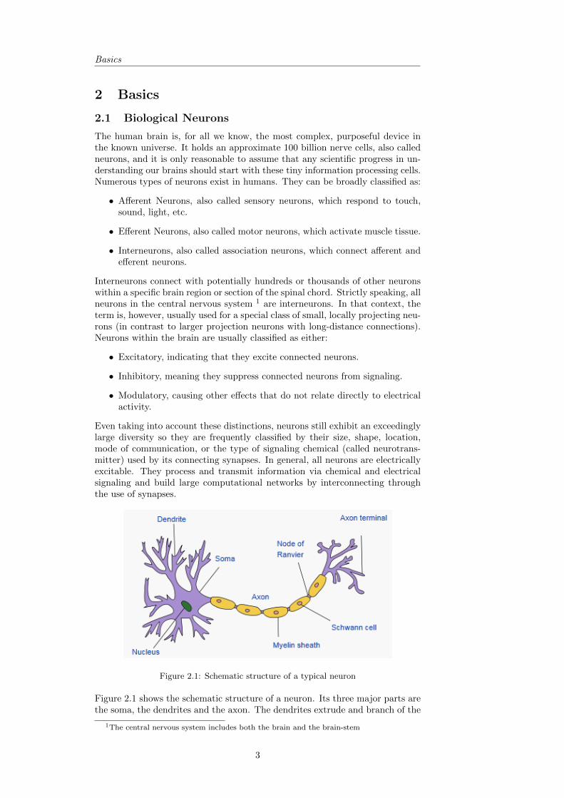
Figure 2.1: Schematic structure of a typical neuron
Figure 2.1 shows the schematic structure of a neuron. Its three major parts arethe soma, the dendrites and the axon. The dendrites extrude and branch of the
1The central nervous system includes both the brain and the brain-stem
3
Biological Neurons
main cell body (soma) dividing further and further into hundreds of ever finerbranches. They only reach a few hundred micrometers from the soma, while theaxon, of which there is usually only one per neuron, can reach very far (up toone meter in certain kinds of neurons) and often branches several times, end-ing in axon terminals for connecting to multiple synapses. While dendrites aremostly used to pick up information from their multiple synaptic connections,the axon is used for transmitting an electric signal away from the cell body tosome other cell. If the length of the axon becomes comparatively long, they arefrequently insulated with sections of a special fatty myelin sheath formed by socalled schwann or glia cells. These sheaths increase the electrical transmissionspeed by up to a hundredfold while reducing the required energy. Adult hu-mans have approximately 149,000 km of myelinated axons in their brains. Lossof myelin or demyelination (as characteristic for multiple sclerosis) thus directlyresults in the inability of cells to communicate with each other by effectivelybreaking the electrical signaling chain.
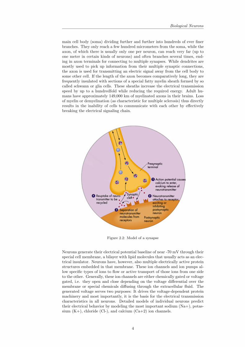
Figure 2.2: Model of a synapse
Neurons generate their electrical potential baseline of near -70 mV through theirspecial cell membrane, a bilayer with lipid molecules that usually acts as an elec-trical insulator. Neurons have, however, also multiple electrically active proteinstructures embedded in that membrane. These ion channels and ion pumps al-low specific types of ions to flow or active transport of those ions from one sideto the other. Generally, these ion channels are either chemically gated or voltagegated, i.e. they open and close depending on the voltage differential over themembrane or special chemicals diffusing through the extracellular fluid. Thegenerated voltage serves two purposes: It drives the voltage-dependent proteinmachinery and most importantly, it is the basis for the electrical transmissioncharacteristics in all neurons. Detailed models of individual neurons predicttheir electrical behavior by modeling the most important sodium (Na+), potas-sium (K+), chloride (Cl-), and calcium (Ca+2) ion channels.
4
Basics
While certain sensory neurons may trigger upon stretch, pressure, light orother external stimuli, neurons in the brain are usually activated through theirsynapses. The synaptic transmission is triggered by an action potential whichdenotes a propagating wave of depolarization (an electrical signal approximately100 mV above the baseline) that activates the release of specific neurotransmit-ter chemicals when it reaches the axon terminals. Several neurotransmittersare important. The large majority of neurons, however, use either glutamate orGABA (γ-aminobutyric acid). Glutamate is generally excitatory, while GABAhas generally inhibitory effects.
The likelihood of a neuron firing (or changing its firing frequency) thus roughlydepends on what all connected neurons contributed in total to the membrane po-tential. A single synapse is usually incapable of activating a neuron. Dependingon the efficacy of the synapses, the amount of excitatory and inhibitory inputs,it may take several dozen excitatory inputs to pass the action potential thresh-old and cause the postsynaptic neuron to fire. In other words, neuronal firingtypically represents a thresholded sum of synaptic inputs. This mathematicalidealization has, in fact, been used for the development of the first artificialneural networks (see Section 2.5). While some synapses are also classified mod-ulatory, causing long-lasting effects not directly related to the firing rate, theoverall observational conclusion remains:
Neurons interact through their synapses. 2
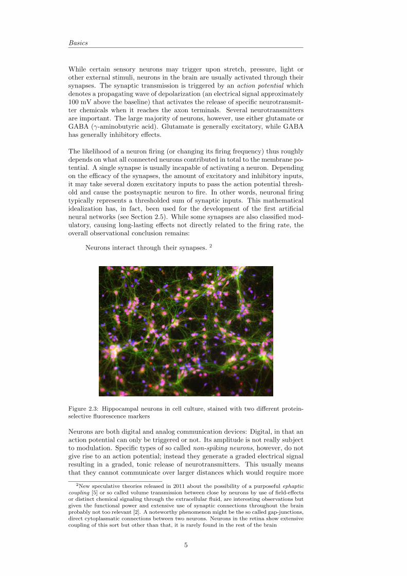
Figure 2.3: Hippocampal neurons in cell culture, stained with two different protein-selective fluorescence markers
Neurons are both digital and analog communication devices: Digital, in that anaction potential can only be triggered or not. Its amplitude is not really subjectto modulation. Specific types of so called non-spiking neurons, however, do notgive rise to an action potential; instead they generate a graded electrical signalresulting in a graded, tonic release of neurotransmitters. This usually meansthat they cannot communicate over larger distances which would require more
2New speculative theories released in 2011 about the possibility of a purposeful ephapticcoupling [5] or so called volume transmission between close by neurons by use of field-effectsor distinct chemical signaling through the extracellular fluid, are interesting observations butgiven the functional power and extensive use of synaptic connections throughout the brainprobably not too relevant [2]. A noteworthy phenomenon might be the so called gap-junctions,direct cytoplasmatic connections between two neurons. Neurons in the retina show extensivecoupling of this sort but other than that, it is rarely found in the rest of the brain
5
Biological Neurons
discrete, spiking forms of communication. However, even spiking neurons maycommunicate in a form of analog mode by modulating their firing-frequency.
We are born with approximately 100 billion neurons. Despite a controversy in1999 after a discovery of some rare form of neurogenesis in the neocortex of theadult brains, recent research reaffirmed that basically all neurons in the adultbrain were formed before birth and are never replaced [47]. Given that neuroge-nesis was found and repeatedly confirmed out of all places in the hippocampalregion, potentially poses a problem: The hippocampus holds a special relevancefor this thesis and even limited neurogenesis might play a not yet clearly deter-mined role in memory function. Considering the overall numbers, it is still fairto say, however, that brain neurons are the only types of human body cells thatremain unreplaced until death. With 100 billion neurons in the human brainand several thousand connections per neuron, it has been estimated that afterthe massive synaptic buildup in the first few years, a three-year-old child hasabout 1015 developed synapses (1 quadrillion). After that, neuronal connectiv-ity decreases until it stabilizes again in adulthood at an approximate 100 to 500trillion synapses. Nevertheless, the brain retains a large degree of neuroplasticity(see Section 2.1.2). By that term we mean the ability of neurons to remove ex-isting synaptic connections, weaken or strengthen existing connections, or evenform entirely new synapses (more on this topic in Section 2.1.2).
2.1.1 Neural and Synaptic Depression
Since many neurons generate their firing capability through the active buildupof a large action potential, there is often a resting period within which the neu-ron can not fire again, while it’s ion pumps are repolarizing the neuron. Thiseffect is called the refractory period. Together with other neural effects suchas an intermittently exhaustive supply of neurotransmitter (re-uptake of spentneurotransmitter also takes time) and decreased responses after repeated acti-vations, this is also called neural depression.
Synaptic depression on the other hand denotes the reduced ability of a synapseto communicate to another cell. There are many effects that are discussedas contributing to synaptic depression. Chief among them is an effect calledLong-term depression (LTD), an activity-dependent reduction in the efficacy ofneuronal synapses lasting hours or days. This is the exact functional opposite ofLong-term potentiation (LTP), a highly studied effect that will be explained infurther detail in Section 2.1.2. Unlike inhibitory and adaptive mechanisms thatreduce responsiveness to all inputs (neural depression), synaptic depression isinput-specific. Both neural and synaptic depression play an important part inthe computational neural network model introduced in Section 2.6 and following.
2.1.2 Neural Plasticity and the Neurological Basis for Memory
To answer the question, where the neurological basis for memory is to be found,how the brain physically stores information, we have to turn to neural plasticity.What exactly do we mean by that term? In their book ”Toward a theory ofneuroplasticity”, Christopher A. Shaw and Jill C. McEachern coined it as:
[...]the ability of the brain and nervous system in all species to changestructurally and functionally as a result of input from the environ-ment. [64]
In a broad sense, neuroplasticity is the basis for all neurosciences because thestudy of the nervous system revolves around changing properties of neural el-ements. These may be caused by natural or artificial alterations of the input,neural trauma or as a part of natural development processes [64]. Given that
6

Basics
the number and position of neurons does not change significantly during adultlife, much of the research attention has been focused on the many processesunderlying the growth of dendrites, axons, changes in electrical characteristics,and synaptic connections.
Given the central importance of neuroplasticity, an outsider wouldbe forgiven for assuming that it was well defined and that a ba-sic and universal framework served to direct its current and futurehypothesis and experimentation. Sadly, however, this is not thecase. While many neuroscientists use the word neuroplasticity asan umbrella term it means different things to different researchersin different subfields. Relatively few workers have seemingly beenwilling or able to look beyond their own quite reductionist modelsof neuroplasticity, to probe for similarities or differences in othermodels. In brief, a mutually agreed upon framework does not exist.[64]
This rather bleak outlook on finding a consistent theory for describing neuro-plasticity in 2001 has improved considerably throughout the last decade.3
For the purpose of this thesis, neuroplasticity denotes lasting activity-dependent(Hebbian) changes in synaptic connectivity within a set population of neuronsand in between several populations of neurons. What exact biomolecular mech-anisms govern these changes is not of concern to this thesis. What is, however,extremely important, is the kind of changes to be modeled by an artificial com-putational neural network, and that these changes are directly caused by theneural input.
A key term for describing this phenomenon is long-term potentiation (LTP) [9].It denotes an observed effect of synaptic strengthening between two neuronsthat results from stimulating them synchronously or shortly after another. Thisphenomenon is of fundamental importance, given that memories are thought tobe encoded in synaptic strength and synapses (not neurons!) are thus the truebiological basis for memory.
The first researcher to suggest that learning may not require the formation ofnew neurons was the Spanish neuroanatomist Santiago Ramon y Cajal. Famousfor his technique of staining neurons with ink, he proposed that memories couldbe formed by changes in the synaptic connectivity between neurons. A mostimportant theoretical expansion of this idea was introduced by Donald Hebbin 1949, a man who is nowadays known as the father of neuropsychology andartificial neural networks. In his book, ’The Organization of Behavior’, Hebbsuggested that cells may grow entirely new connections in addition to metabolicchanges that increase the effectiveness of specific synapses. This comprehen-sive book was the first attempt to unite the higher functions of mind with itsbiological basis and is nowadays seen as a sort of bible for neuroscientists.
When an axon of cell A is near enough to excite cell B and re-peatedly or persistently takes part in firing it, some growth processor metabolic change takes place in one or both cells such that A’sefficiency, as one of the cells firing B, is increased. [23]
This legendary postulate has often been paraphrased as a rhyme: Neurons thatfire together, wire together. Hebb’s Rule governs how synaptic strength inside a
3In part, due to increasing attempts to bind together theories, as undertaken by Shaw andMcEachern themselves and the larger idea of creating a brain theory such as advocated byAI-researcher Jeff Hawkins [22]
7

Biological Neurons
neural population (that Hebb referred to as cell assemblies) changes dependingon the activation patterns. Hebb laid out how a neural network governed bysuch a rule could perform learning, memory and certain kinds of computation.
Because this learning rule is the fundamental basis for artificial neural networks(ANN), we will revisit Hebb’s Rule in Section 2.5.
In life-tissue, LTP was first observed in 1966 in the Oslo, Norway by TerjeLømo, while he ran a series of neurophysiological experiments on anesthetizedrabbits in a research effort involving the hippocampal formation. His researchwas motivated by the investigation of neural plasticity. He was not investigatingthe hippocampus for its potential relevance in memory. The link between LTPand memory was actually made years later in collaboration with other scien-tists (Bliss, Andersen). What he found –rather accidentally– was that whenhe stimulated presynaptic fibers in a certain area, he would not only recorda response from an array of postsynaptic cells due to excitatory postsynapticpotentials. Rather, he observed that the recorded response to singular pulseswould be enhanced if it was proceeded by a train of high-frequency stimuli tothe presynaptic fibers. And furthermore, this enhancement would last for hours.Repeated activations would somehow cause a long-lasting enhancement of theneural response. This effect would later be called long-term potentiation. Asimple Google N-Gram search reveals, that LTP-related research grew expo-nentially in the three decades following this discovery and by the end of thecentury Robert Malenka estimated in an address to the US Society of Neuro-science, that it alone accounts for roughly four papers a day [35].
Short-term memory effects (sometimes called Early-LTP) are based on quick,but transient functional synaptic change on the timescale of a few minutes.Through repetition, these may also trigger a biomolecular cascade that finallyleads to specific changes in gene-expression (Late-LTP) in individual neurons,which then gives rise to protein synthesis 4. Protein synthesis is requiredfor long-term memory because it involves lasting changes in synaptic connec-tions such as the physical formation of more receptors or even completely newsynapses. The exact bio-molecular signal-transduction pathway is complicated,nowadays mostly understood, but still a current research focus. Take a look atFigure 2.4 for a simplified sketch of the signal transduction pathway of LTP inan hippocampal area called CA1 (we will get back to this critically importantbrain region in Section 2.3.3).
In addition to the specificity of the response, required by Hebb postulate, thereis also associativity generated as a direct result of LTP (see Figure 2.5). Tosee how this comes about, consider that LTP is only triggered at a synapse ifthe input caused a high enough change in the excitable post synaptic poten-tial (EPSP) to trigger the post synaptic neuron. So a repeated activation of aweak synapse might not yield a strengthened synapse, because LTP was neverinitiated. Next, consider that a second rather strong synapse, terminating atthe same neuron, is activated repeatedly at the same time. LTP will be initi-ated through the large EPSP-effect of the strong synapse and because the weaksynapse now took part in activating the post synaptic neuron (preceding 5 it
4Molecular neurobiolgogists often draw the line between LTM and STM by simply askingthe question, whether a memory effect involves protein synthesis or not.
5As it turns out, this is were neurobiology deviates from Hebb’s rule: Associative strength-ening (LTP) only occurs if the weak stimulus precedes the strong stimulus. If it comes afterthe fact, the effect is actually opposite, generating LTD and a reduced efficacy of the weaksynapse. This remarkable composition of opposing effects is called spike time dependentplasticity (STDP). STDP implements a form of temporally graded associated learning thatrewards perceived causality and its mechanism was shown by Eccles to be reflected in Pavlo-
8

Basics
Figure 2.4: Signal-transduction for LTP in the hippocampal CA1-region
Figure 2.5: LTP-Specificity and Associativity
ca. 0-40ms), not only does the strong synapse get strengthened but also theoriginally weak synapse.
Associative learning is a key part of many learning system principles. PavlovianConditioning is the most straight forward example for this, but there are manymore. It can be argued that in an LTP-capable neural network, the input itselfcauses lasting (and even predictable) changes in the neural network topology.Many questions regarding the processes of neural plasticity are still unanswered.It has however become abundantly clear that LTP and its functional opposite,LTD (long-term depression), are indeed the fundamental neurological basis forbiological memory 6.
vian conditioning: Only if the bell (weak stimulus) rings before the meat (strong stimulus)is presented, will the dog learn to associate the two such that the bell alone can now triggersalivation. If the bell is rung after the meat has been presented, no conditioning occurs.
6The evidence is particularly strong for declarative memory, such as spatial maps in theCA1 region of the hippocampus (see Section 2.3.3)
9

Human Memory
2.1.3 Dopaminergic Plasticity Modulation
As mentioned in the Section 2.1.2, LTP involves triggered gene expression. An-imal studies [32] have found that the activation of gene transcription factors inLTP can be modulated by dopamine. This can be interpreted as meaning thatno long-term effects (which require protein synthesis and thus genetic expres-sion) can come about without certain dopamine levels, or the other way around,that dopamine enables learning. Dopamine can thus be said to modulate neuralplasticity.
2.2 Human Memory
The question of human memory, how and why certain memories are acquiredand eventually forgotten or become life-long memories instead, has fascinatedphilosophers long before cognitive psychologists and somewhat later neurosci-entists gathered the first real clues on how the brain accomplishes successfulmemory function. After the field had been restricted for hundreds of years tophilosophers only and their rather imaginative but inaccurate conceptions aboutwhat memory is and how it works, it were only the first experimental clinicalstudies in psychology that started to reveal details on what memory really is.
Human memory is to us first and foremost, the ability to store previously expe-rienced information for later usage and then successfully retrieve it. We speak ofmemory impairments if either storage or retrieval are flawed. As such, memoryis defined by a dual functionality and it not easy to distinguish the two by mereobservation. But contrary to common perception, memory is much more thansimple storage and retrieval and if we can indeed vividly relive the past throughour memory, then it is still a very redacted, compressed and highly edited ver-sion of the real present experience. The tools of functional brain imaging 7,clinical studies and animal models enabled nowadays brain sciences to achievedramatic discoveries into the organization of human memory over the course ofa few decades. Discoveries were made that had eluded our self-introspection,logical analysis and psychological studies for centuries.
But before we get into details, we should set ourselves straight on anotherdefinition. What is memory? While it can be argued, that any change followingan experience is memory, it is much more useful to restrict that notion a bitfurther. I shall therefore refer to the Israeli neurobiologist Yadin Dudai, whodefined memory as:
[...]the retention of experience dependent internal representationsover time. [11]
2.2.1 Taxonomy of Memory
Contrary to the first memory theories that treated memory as a unitary sys-tem, human memory is not just one large storage block in some section ofthe brain. In fact, we have several modules and various brain sections par-ticipating in different and even independent forms of memory. What is mostrelevant in the context of this thesis, is the distinction between short-term mem-ory (STM) and long-term memory (LTM), first introduced by William James
7Functional brain imaging techniques, such as functional Magnetic Resonance Imaging(fMRI) , Magnetoencephalography (MEG), Positron Emission Tomography (PET) or SinglePhoton Emission Computed Tomography (SPECT), enable neuroscientist to visualize directlyand often in real time, where exactly neural tissue is electrically active, metabolizes certainchemical elements or generally consumes energy. Given the success and fast improving spatialand temporal resolution of these techniques, potential applications for thought-identificationor mind-reading have become a controversial issue.
10

Basics
in 1890. It was extended by Atkinson and Siffrin in 1968 into the so calledmulti-store-model. There are numerous neurophysiological cases supporting theSTM-LTM separation, such as cases of highly impaired STM with preservedLTM-functionality [63] and other cases of severely degraded LTM with unaf-fected STM performance [62]. From a neurological perspective, STM, as in re-
Figure 2.6: The multi-store model as introduced by Atkinson and Shiffrin in 1968.
membering what we just saw or heard mere seconds ago, is activity-dependent.Its contents are stored in the present neural activity itself in forms of maintainedfiring (-frequency) of coalitions of neurons, even after the original stimulus isgone. This form of memory is very fast and essentially learning in real-time buthighly limited in its capacity and very volatile: New sensory information, themere passage of time (without active rehearsal) or a sudden blow to the headcan quickly erase its contents. [30, p.196-204]
Unlike the RAM in a computer, there is not a singular STM block in the brain.The Atkinson-Shiffrin-model in Figure 2.6 was criticized for presenting it asunitary. In fact, the different sensory modalities each have their own memorycapacity. For these and other reasons, psychologists have replaced the termshort-term memory with working memory (WM), which consists of a centralexecutive (directing the attention) and several slave memory-modalities workingin parallel.
Figure 2.7: The working memory model, as introduced by Baddeley and Hitch in 1974
For example, it has been argued [6] that we have a phonological loop (see Fig-ure 2.7) for storing language. We utilize this temporary auditory buffer torepeat the last uttered phrases to ourselves. This automatic storage can evenbe surprisingly unconscious to us: Sometimes we kindly ask a speaker to repeatwhat he just said, assuming that we did not understand acoustically, only tobe surprised that by playing back and reprocessing the phonological loop inour mind, we suddenly do understand what was just said before the speakercan even repeat his words. Likewise, we have a visual buffer or scratchpadfor visual information. We can even transfer written/visual language into thephonological-loop by silently articulating the words to our inner ear. We oftendo this when we try to remember a phrase or a list of named items, because
11

Human Memory
active rehearsal inside the phonological loop is very reliable 8. Working mem-ory(WM) is essential for intelligence 9 and even simple task, like addition ofnumbers, comparing the hue of two objects, copying a word or filling out a formwould be impossible without WM.
2.2.2 Long-Term Memory Classifications
What about long-term memory then? Much like STM, LTM is not a unitarysystem. In fact LTM comes in even more flavors and clearly multiple levelsof distinctions are necessary to account for different kinds of learning, distinctforms of amnesia and LTM disorders.
The first major distinction is commonly phrased as the difference between know-ing how and knowing that. First laid out by Squire and Cohen in 1980 [8, 69],procedural and declarative memory respectively are distinguished most easilyby the fact that declarative memories can be consciously recollected (such asremembering facts), whereas procedural memories remain inaccessible to direct,conscious recall (i.e. such as explaining how to ride a bicycle). The validity ofthis important distinction is most drastically shown in cases of amnesia, wherepatients retain full procedural memory function without any lasting consciousrecollection of having learned them. A rather impressive example is the case ofthe musician Clive Wearing.
A gifted musician and scholar, he suffered a viral brain infection thatalmost killed him and destroyed parts of both temporal lobes. Hiscase is extremely severe, both in the extend of retrograde amnesia–he has only the haziest idea of who he is– as well as in his inabilityto learn anything new. His musical capacities have largely remainedhowever. [30, p.194]
Other than skills, procedural memory (sometimes also referred to as non-declarativememory) also encompasses classical conditioning, priming (the increased prob-ability of retrieving a recently observed memory), adaptation (i.e. masking ofstimuli by repeated similarity), sensitization (amplification of a response follow-ing repeated stimuli) and habituation (i.e. desensitization to low-level-noise),which shall not be explained in any further detail here because the real focusof this thesis will be on declarative memory, the other branch of LTM. It isquite obvious from the diversity of non-declarative memory functions, that thisis by itself a non-unitary system spread over many brain areas (see Section 2.3.2)
What most people think of, when asked about memory, is declarative memory:The conscious recollection of facts or events from their past. In line with thisthinking, several taxonomies of memory, such as the classifications laid out byZola-Morgan and Squire in 1991, divide declarative memory into episodic andsemantic memory (see Figure 2.8). Episodic memories are concerned with pastevents and their relationship to one another, while semantic memory constitutesabstract, factual knowledge. These can be interlinked of course, as in when weremember where and how we learned of a fact. But most often, our semantic
8unless we have to talk to someone else, interrupting attention to the articulatory repetitionfor too long.
9In fact, WM capacity is highly correlated with IQ-test performance. Comparative mea-surement of WM capacity is most often done by calculating a so called memory-span [42].That is the number of specified items that can be stored in the specific working-memory. Foran example most people can store seven to nine digits in the phonological loop. We notice thecapacity limitation when we try to remember a phone-number longer than this for writing itdown. New research puts the memory-span at about three to four items but by chunking someitems together, as in remembering triplets instead of single digits, we can extend capacity abit.
12

Basics
Figure 2.8: Memory Taxonomy by Zola-Morgan and Squire(1991)
knowledge becomes decoupled from the original learning experience. For an ex-ample we know the capital of Russia without knowing for certain how we cameto know that fact. If we did, that would count as an episodic memory.
It should not go unmentioned here that taxonomies like these, or the one laidout by Schachter and Tulving (1994) [61], are based on psychological data.Brain data is only used to verify pre-conceptualized models and there is no finalconsensus on how many distinguishable memory systems there are, how theyall relate to each other, or if some of them should be considered separate atall. For an example, many taxonomies nowadays set autobiographic knowledgeapart as a separate group of declarative memory. More evidence on how manyindependent memory systems there are, is still emerging from a broad range ofanimal studies, clinical cases of amnesia, memory defects and related psycho-logical studies.Cognitive neurobiology is concerned with interlinking these known systems totheir biological basis of neural circuitry inside the brain. Knowledge about brainhierarchy (which brain regions project where?), gathered by detailed analysisof actual brain tissue and modern tools of functional brain imaging are tremen-dously helpful here. But for many parts of the total memory system, there isstill an ongoing debate on where to place them in the brain and what brainsections are involved in memory encoding, storage, reactivation and retrieval.
13
Human Brain Architecture
2.3 Human Brain Architecture
In a speech given at the 250 year anniversary of the University of Columbia, theNobel prize winner in physiology of the year 2000, Eric Kandel, distinguishedtwo major problems of physical memory research:
I. The Molecular Problem of Memory:How is memory stored at each site?
II. The Systems Problem of Memory:Where in the brain is memory stored?
We have visited some key concepts of the molecular problem in Section 2.1.2.Established taxonomies of memory (Section 2.2.1), based in neuropsychologicalresearch, generate the obvious expectation to find functionally different formsof memory physiologically separated as well. In visiting the second problemof memory, we thus need to familiarize us with basic brain anatomy beforewe can face the systems problem (or the rather specific aspects of the systemsproblem, this thesis deals with) with detailed questions about the interactionbetween the involved brain regions, some of which have already been alluded to.
To most of us non-neuroscientists, the brain looks like a giant cauliflower. Butcloser examination reveals that its is indeed highly structured, both physio-logically and functionally. Much like a highly technical device, its differentcomponents reveal a lot about how the brain works.
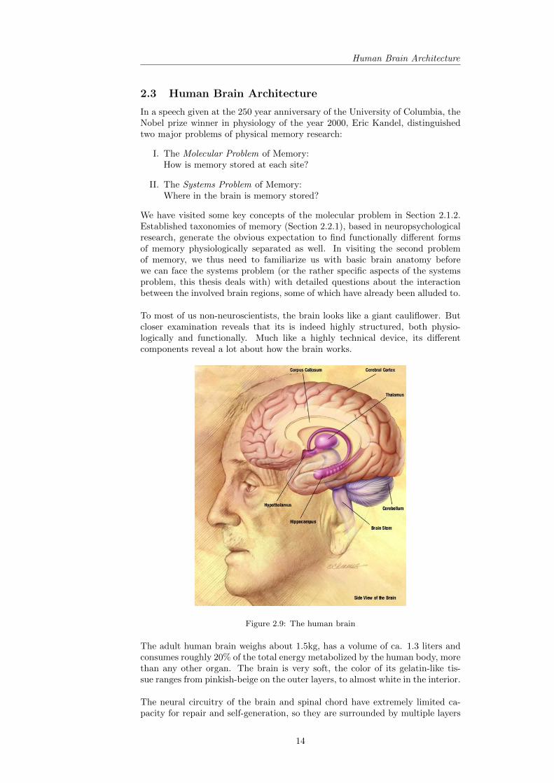
Figure 2.9: The human brain
The adult human brain weighs about 1.5kg, has a volume of ca. 1.3 liters andconsumes roughly 20% of the total energy metabolized by the human body, morethan any other organ. The brain is very soft, the color of its gelatin-like tis-sue ranges from pinkish-beige on the outer layers, to almost white in the interior.
The neural circuitry of the brain and spinal chord have extremely limited ca-pacity for repair and self-generation, so they are surrounded by multiple layers
14

Basics
of protection. The brain is encased in the skull, the spinal cord in the vertebralcolumn. Underneath the bone, a material called dura mater with an inner andan outer layer encases the brain underneath the skull. Beneath that hard matterif the arachnoid, an elastic layer, and then, finally, the pia mater which followsall the small structural details of the highly convoluted topography. All bloodvessels are also insulated by the pia on their way through the cerebrospinal fluid,which suspends the entire brain in liquid and fills the rest of the volume. Thissystem does not only protect the brain from physical injury but also avoids anydirect contact between the blood vessels and the brain, selectively isolating thebrain from most of the body chemistry and preventing otherwise highly danger-ous bacterial infections from reaching the brain [29]. 10
Figure 2.10: The lobes of the cortex
The Cortex is divided into four lobes:
• Frontal lobe
• Parietal lobe
• Occipital lobe
• Temporal lobe
The lobes of the cortex (see Figure 2.10) are not named because they are reallystructurally seperate (with the possible exception of the frontal lobe) but ratherafter the skull-bones underneath which they lie.
The cerebral cortex, divided into two hemispheres, (interconnected by the corpuscallosum, an enormous nerve bundle) is the largest and evolutionary youngestpart of the brain, sitting on top of all other brain structures [29]. The cortex canbe subdivided into the phylogenetically old olfactory and hippocampal cortexand the more recent and much larger neocortex, unique to mammals. Over the
10This is the so called blood-brain-barrier which makes it difficult to administer drugs suchas antibiotics directly to the brain via the blood stream because the barrier does not allowfor the antibiotics to pass from the blood into the cerebrospinal fluid.
15

Human Brain Architecture
course of mammal and primate evolution, its surface area has increased drasti-cally to about 1200cm2 per hemisphere, overshadowing all other brain parts byfar. Lots of envagination are necessary to fit this table-cloth-sized surface intothe brain. Most of the cortical growth came from the addition of the enormousprefrontal lobes which are related to abstract thought, reasoning, planning andother executive functions. This evolutionary trend, called corticalization, madethe cortex indispensable for active life. After surgical removal of the entire cere-bral cortex, less developed mammals, such as rats, can still interact with theenvironment and walk around [73]. Humans will not necessarily die, however,they quickly fall into a permanent state of coma after even partial damage tothe cortex.
The Thalamus is the central relay station before the cortex. [29]. Simply stated:’Nobody talks to the directly cortex’. In fact, the thalamus has a virtualmonopoly on that and without major exceptions, all sensory information hasto pass through the thalamus before it can reach the cortex. Within the thala-mus there are specific nuclei (small rather dense clusters of neurons) for specificsensory modalities such as the lateral geniculate nucleus which relays all datafrom both retinas before it reaches the visual cortex. Whether the thalamus justrouts or to what extend it also processes and integrates separate data-streamsis still a mater of scientific debate.
The Cerebellum is a motor structure that has to do with postural control andbalance. When the sensory information from the skin and joints comes up tothe cerebral cortex, it gives rise to the perception of movement, position, pain,temperature, etc. But as the cerebellum sits directly on top of the brain stem,it has its own method for collecting information and does not need to rely oninformation from the cortex relay. Instead, it takes up duplicate informationfrom the brainstem and uses it to manage postural control and motor coordina-tion. The cerbellum is in that sense seperate from the rest of the brain. It takesinformation up on its own, and it is capable of acting, sending motor signalsdirectly back through the spinal column for fine motor control 11.
2.3.1 Columnar Organization of the Cortex
All of the neocortex is a hierarchical vertical six-layer columnar sheet, only 2-3mm thick (see Figure 2.11) [29]. With ca. 100.000 cells below every squaremillimeter, the neural density is relatively constant. Each layer is unique withrespect to the neuron types that are to be found there and the principled des-tination of their axons.
Layer four is always the input layer from the thalamus, so axons from thalamicneurons terminate in this layer. From there, information is projected to thedensely populated layers two and three, which also integrate information hori-zontally from other cortical areas. From there, neurons are connected to layersfive and six, the only layers that have projection neurons, pyramidal neuronscapable of projecting information back out of the cortex. Layer one is onlysparsely populated and the target of feedback pathways from other cortical ar-eas. It has been framed as a context-providing layer. [30, p.72]
As it turns out, the neocortex is not only a layered structure but also organizedin a columnar fashion:
11In humans at least, the enlarged lateral zones of the cerebellum are highly interconnectedwith the cortex as part of a later evolutionary trend toward corticalization
16

Basics
Figure 2.11: The laminar six-layer structure of cortical columns - only very few neuronsare shown here
In 1957, the American neuroscientist Vernon Benjamin Mountcastle [45] discov-ered that cortical neurons with a horizontal distance of more than 0.5mm fromeach other do not have overlapping sensory receptive fields (meaning they donot respond to the same range of stimuli) while the vertical distance, meaningthe depth in the cortical sheet, did not make much difference. This reflects afunctionally columnar organization: Local connections in the cerebral cortex’up’ and ’down’ the cortical sheet are much denser than side wise connections.
David Hubel and Torsten Wiesel won the 1981 Nobel Prize for their discovery ofneural minicolumns in the visual cortex: Neighbouring columns of much smallersize were found to be similar in their receptive fields. For example, it was shownthat columns with neurons responding to certain angles in an optical stimulus(an angled black bar shown to the eye) were neighboring columns of neuronswith a slightly different receptive field, meaning responsive to a slightly differentangle. In fact, in transversing electrodes at an oblique angle through the cor-tical sheet, they showed that a collection of neighboring columns continuouslyspanned a large space of detection angles. These groups of minicolumns sharinga common thalamic input, selective for different values of the same stimulus,are coding for different values of the same parameter at a specific spot in thereceptive field and were consequently named hypercolumns.
Minicolumns consist of approximately 80 neurons12 of different types, positionedin six distinct layers of the cortical surface. They react to a specific stimulusand neighbor other minicolumns, which responds to a slightly different stimulus.One thalamic input (one axon) reaches about 100-300 minicolumns. 50 to 100minicolumns span the detection space of a specific variable (such as detectingfor the orientation angle in an optical input at a specific spot on the retina) andform a hypercolumn, also referred to as a cortical column. Neighboring columnsare separated by pericolumnar inhibition, so they become very selective in theiractivity.
The columnar theory for the cortex stipulates that this basic layout of six-layercolumns of approximately 0.5mm in width is replicated many times over 13
12with the exception of the much denser V1 area in the visual cortex, for example Macaquemonkey V1 minicolumns are only 31µm diameter but include over 140 pyramidal cells (Peters,1994)
13This is obviously most fascinating to computer engineers who are used to see the develop-
17

Human Brain Architecture
which is why it needs so much surface area. Johansson and Lansner have esti-mated a total number of about two million functional columns for the humancortex [31]. During evolutionary brain growth, the same concept was simplyused again and again to pack more and more columns into the brain. Theentire neocortex is thus remarkably homogeneous and it can be argued thatdifferences between cortical regions are mostly due to their different input (sayvisual information instead of auditory). Because different areas are used forvery different functions, but the hierarchical organization is rather strict, thesix-layer neural column-design only adapts in terms of the thickness of distinctlayers:
Sensory areas for an example, which receive a lot of information from the thala-mus, have typically a very thick layer four (rather drastic in case of the primaryvisual cortex), whereas an association area might have a thiner input layer butmore neurons in the horizontal layers for integrating more information fromother cortical areas.
Long before neuroscientists even knew which cortical area is responsible forwhat, maps listing several dozen areas were compiled based on observable changesin neural density of specific layers between areas. We now know that all of theseareas also correspond to distinct brain functions, confirming the old rule thatstructure and function are correlated. Roughly speaking, the more sensory neu-rons are involved, the bigger the total cortex surface area corresponding to thatbody part or sensory organ.
2.3.2 Specific Memory Areas
Identifying specific bio-molecular processes of memory in neural circuitry (Sec-tion 2.1.2) and taking psychology-based memory taxonomies (Section 2.2.1)with their convincing distinctions by their word means, we still have to pointout where exactly those memory-systems are to be found in the brain.There are strong indications for a link between working-memory and the pre-frontal cortex (PFC). This link was first postulated by C.F. Jacobsen in 1936and several researchers after him have shown that prefrontal lesions in primatesand humans (dorsolateral PFC in particular) severely degrade the capacity toexecute tasks, requiring short-term memory capacity while at the same timesparing normal declarative memory [55, 18]. Moreover, the theory that short-term memory is activity-dependent (meaning that its contents are stored inthe sustained firing patterns of certain neural clusters) was strengthened by re-peated findings of PFC-neurons that sustained their firing pattern during theexact time-delay required by memory task for holding the information. Atthe same time, observed disruptions in firing-consistency of these same neuronswould correlate with failures during the memory test. [19]
Regarding non-declarative memory, current knowledge theorizes, that neuronalstructures for habit, skill learning and retention include the sensory-motor cor-tex, certain basal ganglia structures and the striatum [41]. Priming might bea neocortical phenomenon while motor learning is known to be associated withthe cerebellum [36] and the amygdala –known as the emotional center– is indi-cated to be involved in fear-conditioning.
ment of microprocessors as the attempt to pack as many identical computational elements (beit transistors, gates or entire cores) onto a limited surface, necessitating smaller and smallerelements while natural evolution simply increased the computational surface within a limitedskull to make space for more computational units. The development of multi-core chips withparallel computing power is a rough analog, to the multi-columnar parallel computing powerof cortical tissue
18
Basics
This thesis will not go into any further detail regarding these memory-systems,and what is known about them. Instead we will focus on declarative long-termmemory.
2.3.3 The Medial Temporal Lobe and Hippocampus
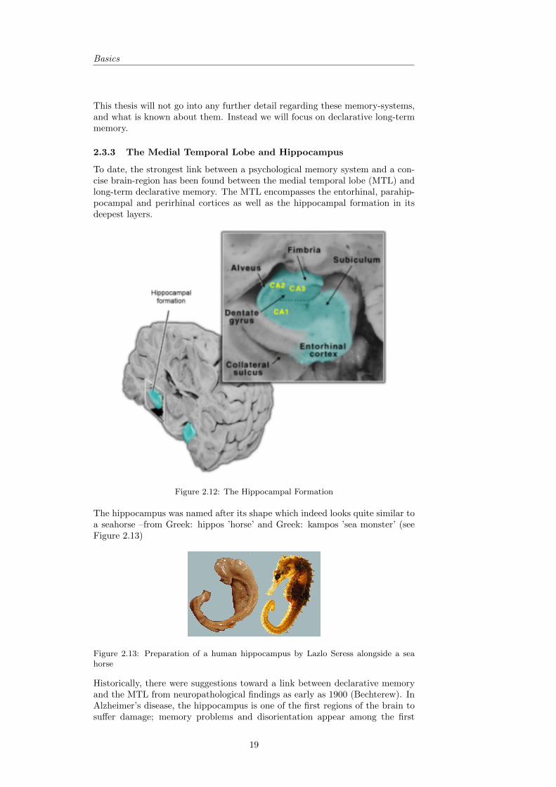
To date, the strongest link between a psychological memory system and a con-cise brain-region has been found between the medial temporal lobe (MTL) andlong-term declarative memory. The MTL encompasses the entorhinal, parahip-pocampal and perirhinal cortices as well as the hippocampal formation in itsdeepest layers.
Figure 2.12: The Hippocampal Formation
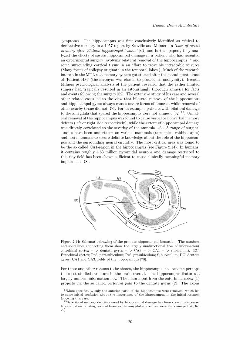
The hippocampus was named after its shape which indeed looks quite similar toa seahorse –from Greek: hippos ’horse’ and Greek: kampos ’sea monster’ (seeFigure 2.13)
Figure 2.13: Preparation of a human hippocampus by Lazlo Seress alongside a seahorse
Historically, there were suggestions toward a link between declarative memoryand the MTL from neuropathological findings as early as 1900 (Bechterew). InAlzheimer’s disease, the hippocampus is one of the first regions of the brain tosuffer damage; memory problems and disorientation appear among the first
19
Human Brain Architecture
symptoms. The hippocampus was first conclusively identified as critical todeclarative memory in a 1957 report by Scoville and Milmer. In ’Loss of recentmemory after bilateral hippocampal lesions’ [62] and further papers, they ana-lyzed the effects of severe hippocampal damage in a patient who had assentedan experimental surgery involving bilateral removal of the hippocampus 14 andsome surrounding cortical tissue in an effort to treat his intractable seizures(Many forms of epilepsy originate in the temporal lobes.). Much of the researchinterest in the MTL as a memory-system got started after this paradigmatic caseof ’Patient HM’ (the acronym was chosen to protect his anonymity). BrendaMilners psychological analysis of the patient revealed that the rather limitedsurgery had tragically resulted in an astonishingly thorough amnesia for factsand events following the surgery [62]. The extensive study of his case and severalother related cases led to the view that bilateral removal of the hippocampusand hippocampal gyrus always causes severe forms of amnesia while removal ofother nearby tissue did not [78]. For an example, patients with bilateral damageto the amygdala that spared the hippocampus were not amnesic [62] 15. Unilat-eral removal of the hippocampus was found to cause verbal or nonverbal memorydefects (left or right side respectively), while the extent of hippocampal damagewas directly correlated to the severity of the amnesia [43]. A range of surgicalstudies have been undertaken on various mammals (rats, mice, rabbits, apes)and non-mammals to secure definite knowledge about the role of the hippocam-pus and the surrounding neural circuitry. The most critical area was found tobe the so called CA1-region in the hippocampus (see Figure 2.14). In humans,it contains roughly 4.63 million pyramidal neurons and damage restricted tothis tiny field has been shown sufficient to cause clinically meaningful memoryimpairment [78].
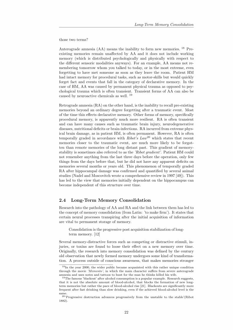
Figure 2.14: Schematic drawing of the primate hippocampal formation. The numbersand solid lines connecting them show the largely unidirectional flow of information(entorhinal cortex − > dentate gyrus − > CA3 − > CA1 − > subiculum). EC,Entorhinal cortex; PaS, parasubiculum; PrS, presubiculum; S, subiculum; DG, dentategyrus; CA1 and CA3, fields of the hippocampus [78].
For these and other reasons to be shown, the hippocampus has become perhapsthe most studied structure in the brain overall. The hippocampus features alargely uniform information flow: The main input from the entorhinal cotex (1)projects via the so called perforant path to the dentate gyrus (2). The axons
14More specifically, only the anterior parts of the hippocampus were removed, which ledto some initial confusion about the importance of the hippocampus in the initial researchfollowing this case.
15Severity of memory deficits caused by hippocampal damage has been shown to increase,however, if surrounding cortical tissue or the amygdaloid complex were also damaged [78, 67,79]
20

Basics
of neurons located there constitute the major excitory input to pyramidal cellsin the CA3-field (3). Neurons in CA3 project exclusively towards field CA1 (4)via a powerful associational connection, called Schaffer Collaterals. From there,neurons project to the subiculum, which completes the circuit by projectingmostly to the entorhinal cortex.[78]
It is not that hard to see, that due to this largely unidirectional structure, thehippocampus does not have a lot of redundancy and it is easy to take downthe entire chain, by removing a single element.16 But does this mean thatinformation is actually stored there? As mentioned in Section 2.2, memory is adual functionality: Storage and retrieval. We could ask whether this signal pathis just critical for retrieval, but the information is actually stored somewhereelse. How would we know? In the 1973, the key pioneers of the field of LTPresearch, Bliss, Gardner-Medvin and Lømo gave their take on it:
From a neurophysiological point of view, a first step in establishingwhether any particular part of the brain is directly involved in theprocess underlying memory (that is, whether it is involved in thestorage and not merely the transmission of learned information) isto look for evidence of synaptic plasticity. [7]
First, experiments have indeed shown high plasticity in the hippocampus. Dueto its predictable, hierarchically strict organization and easily inducible LTP,the CA1 field of the hippocampus has by now even become the prototypical siteof mammalian LTP studies.
Secondly, a most convincing proof or actual storage was the discovery and sub-sequent investigation of place cells. In 1971 O’Keefe and Dostrovsky discovered,that certain neurons in a rats hippocampus fired very selectively whenever therat was in a specific spot of a maze it was to explore [51]. They called theseneurons place cells and hypothesized that the rat hippocampus forms a cogni-tive map of the rats environment. Many studies of this phenomenon have sincebeen conducted and rats running in a maze have indeed been shown to buildrepresentations of spatial maps of the maze-layout within their hippocampus.After a period of learning, these place cells fired vehemently and exclusivelywhen the rat was in a specific spot of the maze. Once formed, these learnedneural maps would be stable for weeks during which the rat may or may nothave learned other mazes as well. These maps are so reliable that in a processakin to mind reading, they allow researchers to predict the position of the ratin the maze with near certainty by only looking at the live-recording of neuralfiring patterns observed via an array of microelectrodes array connected to CA1and CA3 neurons in the rats hippocampus. So at the very least for spatial mem-ory in rats (a form of declarative memory), we have direct proof that storageindeed takes place in the hippocampus. 17
2.3.4 Retrograde and Anterograde Amnesia
Before we can move to the core topic of this thesis, which is memory consoli-dation, we need to clarify one more distinction with regard to memory defects.When patient HM woke up after his MTL surgery, he exhibited two differentkinds of amnesia. Very severe anterograde amnesia and somewhat lighter ret-rograde amnesia, both with respect to facts and events. What do we mean by
16For an example in patient HM, hippocampal damage was restricted to the anterior partbut the effects were still dramatic.
17By now, an entire array of information-coding cells related to spatial orientation wereidentified in specific brain regions: grid cells, border cells, head direction cells, spatial viewcells and others. The entire spacial representation system of the brain is on the verge of beingdecoded. [44]
21
Long-Term Memory Consolidation
those two terms?
Anterograde amnesia (AA) means the inability to form new memories. 18 Pre-existing memories remain unaffected by AA and it does not include workingmemory (which is distributed psychologically and physically with respect tothe different sensoric modalities anyways). For an example, AA means not re-membering tomorrow whom you talked to today, or in the most extreme, evenforgetting to have met someone as soon as they leave the room. Patient HMhad intact memory for procedural tasks, such as motor-skills but would quicklyforget fact and events that fall in the category of declarative memory. In thecase of HM, AA was caused by permanent physical trauma as opposed to psy-chological trauma which is often transient. Transient forms of AA can also becaused by neuroactive chemicals as well. 19
Retrograde amnesia (RA) on the other hand, is the inability to recall pre-existingmemories beyond an ordinary degree forgetting after a traumatic event. Mostof the time this effects declarative memory. Other forms of memory, specificallyprocedural memory, is apparently much more resilient. RA is often transientand can have many causes such as traumatic brain injury, neurodegenerativediseases, nutritional deficits or brain-infections. RA incurred from extreme phys-ical brain damage, as in patient HM, is often permanent. However, RA is oftentemporally graded in accordance with Ribot’s Law20 which states that recentmemories closer to the traumatic event, are much more likely to be forgot-ten than remote memories of the long distant past. This gradient of memory-stability is sometimes also referred to as the ’Ribot gradient’. Patient HM couldnot remember anything from the last three days before the operation, only fewthings from the days before that, but he did not have any apparent deficits onmemories several months or years old. This phenomenon of temporally gradedRA after hippocampal damage was confirmed and quantified by several animalstudies (Nadel and Moscovitch wrote a comprehensive review in 1997 [49]). Thishas led to the view that memories initially dependent on the hippocampus canbecome independent of this structure over time.
2.4 Long-Term Memory Consolidation
Research into the pathology of AA and RA and the link between them has led tothe concept of memory consolidation (from Latin: ’to make firm’). It states thatcertain neural processes transpiring after the initial acquisition of informationare vital to permanent storage of memory.
Consolidation is the progressive post acquisition stabilization of long-term memory. [12]
Several memory-distractive forces such as competing or distractive stimuli, in-juries, or toxins are found to loose their effect on a new memory over time.Originally, the research into memory consolidation was defined by the centuryold observation that newly formed memory undergoes some kind of transforma-tion. A process outside of conscious awareness, that makes memories stronger
18In the year 2000, the wider public became acquainted with this rather unique conditionthrough the movie ’Memento’, in which the main character suffers from severe anterogradeamnesia and uses notes and tattoos to hunt for the man he thinks killed his wife.
19The famous ’blackout’ after alcohol consumption is a popular example. Research suggests,that it is not the absolute amount of blood-alcohol, that blocks the formation of new long-term memories but rather the pace of blood-alcohol rise [21]. Blackouts are significantly morefrequent after fast drinking than slow drinking, even if the achieved blood-alcohol level is thesame.
20’Progressive destruction advances progressively from the unstable to the stable’(Ribot1882).
22
Basics
and more resilient against said disruptions over time even without additionalactive rehearsal. While it may not be accessible to our conscious mind, we arekeenly aware of its existence: Almost two millennia ago, the Roman rhetoricianQuintilian describes his wonder of memory consolidation through sleep:
It is astonishing how much strength the interval of a night gives it,and a reason for the fact cannot be easily discovered [...] It is certainthat what could not be repeated at first is readily put together onthe following day, and the very time which is generally thought tocause forgetfulness is found to strengthen the memory. [56]
We will talk more about the role of sleep in Section 2.4.1. In light of newanatomical studies of amnesia (such as HM) and their direct implications forlocating crucial pieces of the systemic workings of memory consolidation pro-cesses, the field of system memory consolidation gained new momentum in the1960s and 70s. We now know that consolidation most certainly spans all sensorymodalities and various forms of memories, declarative and procedural memoriesand beyond: From motor-learning and fear-based emotional memories to spatialand contextual understanding, involving multiple brain areas. The science getscomplicated by the fact that there is no real consensus on what processes arecovered by memory consolidation and even if researchers agree on a definitionsuch as the one by Dudai, quoted above: How we would find, identify, separateand functionally describe all processes relevant to that description?
Memory researchers generally differentiate between synaptic consolidation andsystem consolidation. They correspond closely to the two problems of memoryresearch set out by Eric Kandel (see Section 2.3). The former finishes withina few minutes/hours after the encoding by training was completed. Because itinvolves protein synthesis (see Section 2.1.2) by the corresponding nerve cell, itis not a stricly synaptic phenomenon and might also be called cellular consoli-dation, but as we already learned that plasticity is driven by synaptic activity,the term is still widely used and appropriate.
System consolidation takes weeks or even months to complete and denotes alarger process with many parts highly relevant to this thesis, whereby memoriesare reorganized, traces get created and diminished in various brain regions, inte-grated with previous knowledge and strengthened into a long lasting interferenceresistant form.In the context of this thesis we are obviously most interested in the highlystudied and seemingly central role of the hippocampus for long-term-memoryconsolidation of declarative memory (what Dudai refers to as System Consol-idation [12]). For the purpose of this thesis, we thus narrow the definition ofmemory consolidation considerably:
Memory Consolidation is a process by which memories that initiallydependent on the hippocampus become progressively independentof that structure over time.
This is supposed to be both the reason for RA and AA after hippocampal lesion-ing: Without the hippocampus, recent memories depending on it are lost (RA)and on top of that, the formation of new long-term memories becomes impossi-ble (AA) because it requires consolidation, which is driven by the hippocampus.Since non-declarative memory is remarkably spared major damage in almost allcases of amnesia directly related to hippocampal damage, we can assume thatthe hippocampus is not directly relevant to non-declarative consolidation.
The standard model of system consolidation is depicted in a flowchart[see also quoted Figure 2.16]. Initial storage, i.e., encoding and reg-istration of the perceived information (Dudai 2002a), occurs in both
23

Long-Term Memory Consolidation
Figure 2.15: Types of consolidation. (A) The time course of synaptic (cellular, local)consolidation, determined by measuring the sensitivity of memory to the inhibition ofprotein synthesis. Consolidated memory is defined as treatment-resistant long-termmemory. The data are from experiments on shuttle-box learning in the goldfish (Agra-noff et al. 1966). The protein synthesis inhibitor was administered to separate groupsof fish at the indicated time points after training. The sensitivity of memory to proteinsynthesis inhibition was over by about one hour. A consolidation process that dependson protein synthesis during and immediately after training is a universal property ofthe nervous system. (B) The time course of system consolidation, determined by mea-suring the sensitivity of long-term memory to hippocampal damage. The data are fromexperiments on contextual fear conditioning in the rat (Kim & Fanselow 1992). Thelesion was inflicted to separate groups at the indicated time points after training. Thedependence of long-term memory on the hippocampus in this case was over by aboutone month. System consolidation, lasting weeks or longer, during which the memorybecomes independent of the hippocampus, is observed in declarative memory. [12]
the hippocampal system and the neocortical system. Sh(0) andSc(0) represent the strength of the initial hippocampal and neo-cortical traces, respectively. These traces are expected to differ,with the hippocampal one probably representing a compressed ver-sion of the internal representation. The hippocampal representationlater becomes active either in explicit recall, or in implicit processessuch as sleep. This gives rise to reinstatement of the correspondingneocortical memory, resulting in incremental adjustment of neocor-tical connections, probably involving local, synaptic consolidation.In parallel, memory also decays, faster in the hippocampus (Dh)than in the cortex (Dc). The net result is that memories initiallydependent on the hippocampus gradually become independent of it.In reality this happens over weeks or longer. The hippocampal sys-tem can hence be viewed not only as a memory store but also asa teacher of the neocortical system. This process (C, rate of con-solidation) is proposed to allow the hippocampal system to rapidlylearn new information without disrupting old memory stored in theneocortex, while at the same time allowing gradual integration of thenew information into the older, structured information. [12, p.62]
In light of this systemic architecture, the cortical system is specialized in theextraction of shared structure in a perceived chain of events. To facilitate anintegration of new and altered concepts into that structure without risking catas-trophic interference, the cortical system will need to be very slow in learning (A
24
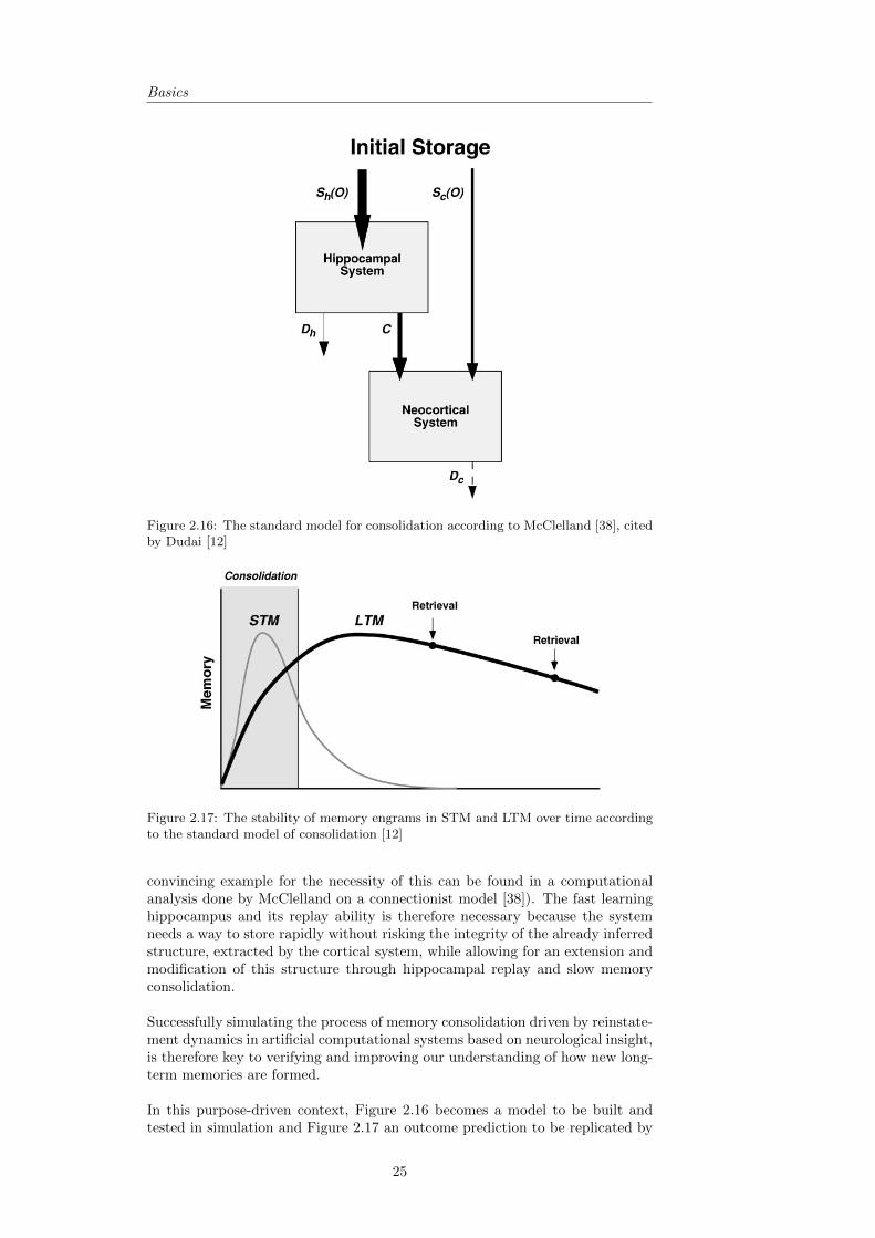
Basics
Figure 2.16: The standard model for consolidation according to McClelland [38], citedby Dudai [12]
Figure 2.17: The stability of memory engrams in STM and LTM over time accordingto the standard model of consolidation [12]
convincing example for the necessity of this can be found in a computationalanalysis done by McClelland on a connectionist model [38]). The fast learninghippocampus and its replay ability is therefore necessary because the systemneeds a way to store rapidly without risking the integrity of the already inferredstructure, extracted by the cortical system, while allowing for an extension andmodification of this structure through hippocampal replay and slow memoryconsolidation.
Successfully simulating the process of memory consolidation driven by reinstate-ment dynamics in artificial computational systems based on neurological insight,is therefore key to verifying and improving our understanding of how new long-term memories are formed.
In this purpose-driven context, Figure 2.16 becomes a model to be built andtested in simulation and Figure 2.17 an outcome prediction to be replicated by
25
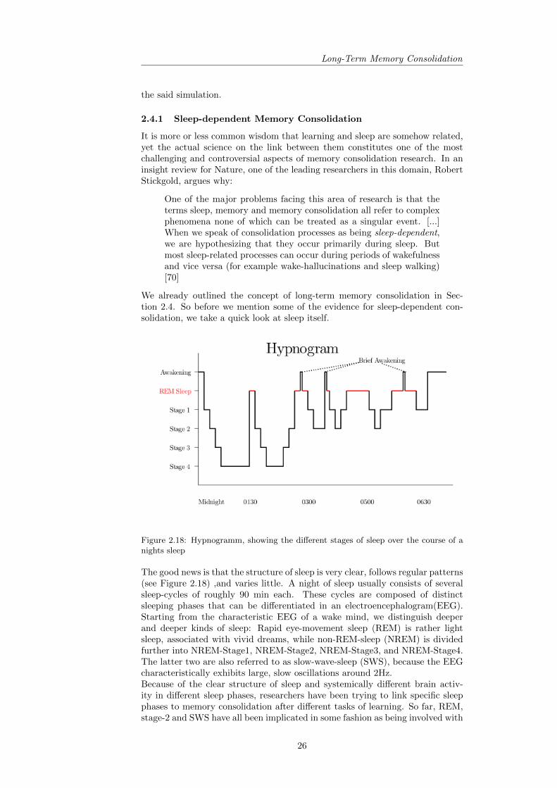
Long-Term Memory Consolidation
the said simulation.
2.4.1 Sleep-dependent Memory Consolidation
It is more or less common wisdom that learning and sleep are somehow related,yet the actual science on the link between them constitutes one of the mostchallenging and controversial aspects of memory consolidation research. In aninsight review for Nature, one of the leading researchers in this domain, RobertStickgold, argues why:
One of the major problems facing this area of research is that theterms sleep, memory and memory consolidation all refer to complexphenomena none of which can be treated as a singular event. [...]When we speak of consolidation processes as being sleep-dependent,we are hypothesizing that they occur primarily during sleep. Butmost sleep-related processes can occur during periods of wakefulnessand vice versa (for example wake-hallucinations and sleep walking)[70]
We already outlined the concept of long-term memory consolidation in Sec-tion 2.4. So before we mention some of the evidence for sleep-dependent con-solidation, we take a quick look at sleep itself.
Figure 2.18: Hypnogramm, showing the different stages of sleep over the course of anights sleep
The good news is that the structure of sleep is very clear, follows regular patterns(see Figure 2.18) ,and varies little. A night of sleep usually consists of severalsleep-cycles of roughly 90 min each. These cycles are composed of distinctsleeping phases that can be differentiated in an electroencephalogram(EEG).Starting from the characteristic EEG of a wake mind, we distinguish deeperand deeper kinds of sleep: Rapid eye-movement sleep (REM) is rather lightsleep, associated with vivid dreams, while non-REM-sleep (NREM) is dividedfurther into NREM-Stage1, NREM-Stage2, NREM-Stage3, and NREM-Stage4.The latter two are also referred to as slow-wave-sleep (SWS), because the EEGcharacteristically exhibits large, slow oscillations around 2Hz.Because of the clear structure of sleep and systemically different brain activ-ity in different sleep phases, researchers have been trying to link specific sleepphases to memory consolidation after different tasks of learning. So far, REM,stage-2 and SWS have all been implicated in some fashion as being involved with
26
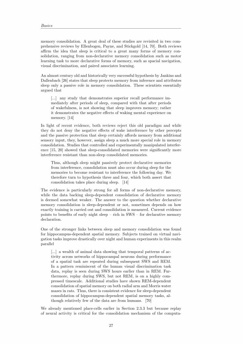
Basics
memory consolidation. A great deal of these studies are revisited in two com-prehensive reviews by Ellenbogen, Payne, and Stickgold [14, 70]. Both reviewsaffirm the idea that sleep is critical to a great many forms of memory con-solidation, ranging from non-declarative memory consolidation such as motorlearning task to more declarative forms of memory, such as spacial navigation,visual discrimination, and paired associates learning.
An almost century old and historically very successful hypothesis by Jankins andDallenbach [26] states that sleep protects memory from inference and attributessleep only a passive role in memory consolidation. These scientists essentiallyargued that
[...] any study that demonstrates superior recall performance im-mediately after periods of sleep, compared with that after periodsof wakefulness, is not showing that sleep improves memory; ratherit demonstrates the negative effects of waking mental experience onmemory. [14]
In light of recent evidence, both reviews reject this old paradigm and whilethey do not deny the negative effects of wake interference by other perceptsand the passive protection that sleep certainly affords memory from additionalsensory input, they, however, assign sleep a much more special role in memoryconsolidation. Studies that controlled and experimentally manipulated interfer-ence [15, 20] showed that sleep-consolidated memories were significantly moreinterference resistant than non-sleep consolidated memories.
Thus, although sleep might passively protect declarative memoriesfrom interference, consolidation must also occur during sleep for thememories to become resistant to interference the following day. Wetherefore turn to hypothesis three and four, which both assert thatconsolidation takes place during sleep. [14]
The evidence is particularly strong for all forms of non-declarative memory,while the data backing sleep-dependent consolidation of declarative memoryis deemed somewhat weaker. The answer to the question whether declarativememory consolidation is sleep-dependent or not, sometimes depends on howexactly training is carried out and consolidation is measured. Current evidencepoints to benefits of early night sleep – rich in SWS – for declarative memorydeclaration.
One of the stronger links between sleep and memory consolidation was foundfor hippocampus-dependent spatial memory. Subjects trained on virtual navi-gation tasks improve drastically over night and human experiments in this realmparallel
[...] a wealth of animal data showing that temporal patterns of ac-tivity across networks of hippocampal neurons during performanceof a spatial task are repeated during subsequent SWS and REM.In a pattern reminiscent of the human visual discrimination taskdata, replay is seen during SWS hours earlier than in REM. Fur-thermore, replay during SWS, but not REM, is on a highly com-pressed timescale. Additional studies have shown REM-dependentconsolidation of spatial memory on both radial arm and Morris watermazes in rats. Thus, there is consistent evidence for sleep-dependentconsolidation of hippocampus-dependent spatial memory tasks, al-though relatively few of the data are from humans. [70]
We already mentioned place-cells earlier in Section 2.3.3 but because replayof neural activity is critical for the consolidation mechanism of the computa-
27

Long-Term Memory Consolidation
tional model developed in this thesis, we shall dwell on this phenomenon andits biological background a bit.
For example, intracellular in vivo studies demonstrate that neocor-tical neurons spontaneously reactivate during SWS; it is conceivablethat this observable phenomenon leads to strengthening of memorytraces. Several animal studies demonstrate that recently acquired,hippocampus-based memories are replayed during sleep. Interest-ingly, replay of hippocampal memories after spatial navigation hasalso been seen in wakefulness; but during wakefulness, these mem-ories are chronologically replayed backward, whereas during sleepthe patterns are replayed forward. It has been suggested that thesedistinct patterns reflect different roles: whereas initial learning relieson reverse replay, consolidation relies on forward replay.
Recent neuroimaging findings in humans further demonstrate in-creased hippocampal activity during sleep following spatial learn-ing, an increase that was proportional to the degree of overnightbehavioral improvement. Collectively, these studies suggest thathippocampus-dependent memories are reactivated during sleep, andthat this reactivation leads to strengthened memory traces. [14]
It is this very consolidation mechanism of strengthening cortical memory tracesthrough repeated reactivations in replay that will be at the very core of thecomputational model developed in this thesis. Obviously, this thesis is not thefirst to try to do so, but before we can see what is unique and particularly goodabout the replay-model used in this thesis, we will need to turn our attentionto the computational basics behind artificial neural networks in a broader sensein the next section.
28

Basics
2.5 Memory in Artificial Neural Networks (ANN)
We now begin with the computational part of the Basics Chapter. It outlinesthe concept of Artificial Neural Networks (ANN) and how they model biologi-cal memory. This part starts with one of the most known ANNs, the Hopfieldnetwork and moves on to the more complex Bayesian Confidence PropagationNeural Networks (BCPNNs). The following sections deal with the computa-tional core of the model used in this thesis and its origins. They are thus rathertheoretical and conclude in a succinct mathematical description of a modifiedBCPNN as implemented in this thesis (see Section 2.6.8).
ANNs are computational models, inspired by the structure and specific func-tional aspects of biological neural networks. From a highly reductionist, com-putational perspective, neurons can be conceptualized as interconnected thresh-olded summing devices. This was indeed one of the earliest and rather successfulidealizations of neurons made in 1943 by Warren S. McCulloch, a neuroscientist,and Walter Pitts, a logician. According to their paper, ’A logical calculus of theideas immanent in nervous activity’ [40], and other similar conceptualizations,ANNs consist of interconnected artificial neurons, often also called units or nodes(see Figures 2.19 and 2.20). Each input to a unit is weighted with a connectionspecific weight before they are summed. Depending on an activation function,often a threshold-like function such as step functions, sigmoids, etc., an outputof the unit is generated. With the right method for teaching the weights, largernetworks of these units can be used to do certain kinds of computational taskssuch as classification or function approximation. [37]
Figure 2.19: An artificial neuron and its components according to McCulloch andPitts [40]
There are many different types of ANN, but they are usually distinguished bythree parameters [37]:
• The pattern of unit interconnections (Fully connected, partially connected,circular, multiple layers of units,...).
• The learning rule for updating the connection weights (such as Hebbianlearning).
• The activation function f, which converts the weighted input into an out-put activation. This may or may not include a summing of the weightedinputs.
29

Memory in Artificial Neural Networks (ANN)
The similarities to biological neural networks are obvious: Units represent neu-rons; weights represent synaptic strength; summing can be seen as a functionof the neural membrane, as it integrates all the excitatory and inhibitory con-tributions to its potential. Weight-learning-rules model processes of synapticplasticity, and activation functions mimic the thresholded action potential ofreal neurons.
Figure 2.20: Network topology of a fully connected eight unit network (without self-connections)
2.5.1 Basic ANN Memory - The Hopfield Network
One of the simplest and most studied ANNs used for associative memory (mean-ing capable of associative recall) is called the Hopfield network 21. Its units arebinary, taking on values -1 or +1 22 and fully connected, meaning, all unitsconnect to each other with the exception of self-connections. Because its unitsare binary, it can be used to store only binary information: Strings consisting ofthe alphabet {-1,+1} with a total length N equal to the number of units in thenetwork. The network is recurrent and its weights symetric: wij = wji. Thismeans that the weight from unit i to unit j is the same as the weight from unit jto unit i. To store information in its network, the weights of a Hopfield networkare set according to Hebb’s Rule.
wij =
{1N
∑Pp=1 x
pi xpj if i 6= j
0 otherwise(2.1)
In line with Hebb’s idea, the connection weight between two units i and j isincreased by one if the activations xi and xj are the same and decreased if theunits are anti-correlated.The time discrete activation-function is rather simple. First, each neuron icalculates a weighted sum of it inputs.
si(t+ 1) =∑
yi(t)wij (2.2)
The new activation value is then computed from the thresholded sum
yi =
+1 if si(t+ 1) > 1−1 if si(t+ 1) < 1yi otherwise
(2.3)
21Actually, the reason why it has been studied in so much detail is precisely because it is sosimple. Methods from statistical mechanics can be used to analyze its theoretical properties.This does not hold true for most other, more complex classes of ANN.
22Hopfield originally used zero and one, but there are some benefits for the simplicity of themathematical description to distinguish the two binary symbols by their sign instead of theirabsolute value.
30

Basics
A network set up this way can execute associative recall. This is done by initiallysetting the activations of the nodes and then letting the network update itselfby recurrent iterations until it reaches a stable state representing the associatedpattern. This can be done either synchronously (all units at the same time)or asynchronously (one units after another). The units will activate/deactivatethemselves until the network essentially finds the most similar pattern, it wastaught.
The memory capacity of this kind of ANN is quite limited. A Hopfield networkcan store approximately 0.15N activation patterns, where N denotes the numberof interconnected units. Storing too many patterns in the weight-matrix wresults in spurious attractors. Those are unwanted stable states not reflectinga learned pattern. Additionally, already stored patterns become unstable andcan no longer be retrieved.
2.6 Bayesian Confidence Propagation Neural Network (BCPNN)
A BCPNN is a special class of ANN. As the name indicates, its Hebbian learningrule and network architecture can be derived from Bayes’ Rule and the NaiveBayesian Classifier (NBC) in Section 2.6.2. As such, it is a correlation basedmodel anchored in a probabilistic view of learning and retrieval. It takes theconfidence of feature detections into account and generates posterior probabilitydistributions as outcomes.
BCPNNs were first developed as feed-forward networks for classification [25] anddata-mining [52]. When used in a recurrent architecture, these fully connectednetworks give rise to fixed-point attractor dynamics similar to other types ofattractor networks. In fact, with proper choice of parameters, a BCPNN canbe used to functionally replace any Hopfield network. However, as we will see,BCPNNs have several advantages over other types of neural networks that makethem especially interesting for modeling biological neural memory.
2.6.1 The Problem of Catastrophic Forgetting
Most ANNs are implemented in predetermined or even artificially arrangedlearning situations with at least roughly known requirements on capacity andmost often stationary learning environments. In real world learning processes,the number of learning examples can easily exceed the storage capacity of thelearner by orders of magnitudes. Traditional correlation based ANNs suffer fromcatastrophic forgetting (CF) under these circumstances. If a network is shownmore and more patterns to be learned, retrieval of stored patterns degrades untilit often rather suddenly collapses and the network becomes unable to retrieveany stored patterns at all. Obviously, a finite system has finite storage capac-ity 23 and after that capacity has been reached, new information must overwriteold information, effectively interfering with the already stored patterns. If thatinterference is spread equally among all stored patterns, then all patterns willbecome unstable at approximately the same load, leading to CF. The importantfact ,however, is this:
CF is unknown to biological memory.
23That much holds true for the human brain as well. Recent estimates are at around 2.5petabytes (Scientific American Mind - May 2010 Issue), however, only the smallest part ofthat theoretical capacity can be tapped for declarative memory. After all, the brain evolvedas a method of increased survival and not as a means for massive storage of meaningless data.
31

Bayesian Confidence Propagation Neural Network (BCPNN)
The BCPNNs implemented in this thesis are superior to traditional ANNs inthat they do not suffer from CF and can deal with near infinite amounts oflearning examples [59]. They prioritize the storage of recent and novel informa-tion just as we know from working memory psychology (see Section 2.2) andforget organically, indicating they forget learned patterns at different points inthe learning process rather than all at once. It should not go unmentionedhere that there are several modifications of the Hopfield learning rule, known asPalimpsest Memories [48] that can also deal with CF by modulating the learn-ing rate depending on the level of crosstalk from previously shown patterns.
BCPNN-architecture can be made to reflect the biological nature of columnarorganisation in the cortex (see Section 2.3.1). By assigning a network unit toindicate a discrete attribute value (corresponding to a highly selective minicol-umn) and different units in the network to select for all other possible discretevalues of the same attribute, we can lump together all these units (minicolumns)into a hypercolumn. Since BCPNNs have a probabilistic underpinning, and hy-percolumnar activations are normalized, the resulting activation of a hypercol-umn can indeed be interpreted as a discretized probability density function ofits assigned attribute. Since many (discrete valued) attributes constitute a pat-tern, several hypercolumns together form the population of the entire BCPNN.By nature of this approach, the model also reflects the mutual inhibition ofcolumns that regulates the level of activity in the human cortex.
2.6.2 Naive Bayesian Classifier BCPNN
The Naive Bayesian Classifier is a classifier, based on Bayes’ Rule, under the(naive) assumption that the presence of particular features of a class are inde-pendent. It generates a probabilistic classification.We start with Bayes’ Rule:
P (A|B) =P (B|A)P (A)
P (B)(2.4)
Our estimator is supposed to express the probabilities πj of the discrete at-tributes yj given a set x of observed attributes xi. Under the assumption ofindependence of xi, we can express these as:
πj = P (yi|xi) = P (yj)
n∏i=1
P (xi|yj)P (xi)
= P (yj)
n∏i=1
P (xi, yj)
P (yj)P (xi)(2.5)
In order to transfer this into a neural network and use its natural summingproperties for computation, we must transform the products into sums which isachieved by using logarithmic probabilities:
log πj = logP (yi) +
n∑i=1
log
[P (yj , xi)
P (yj)P (xi)
](2.6)
In this form, the equation can be implemented as a single-layer feed forward
network with weights wij = log[P (yj ,xi)P (yj)P (xi)
] and biases βj = logP (yj). The
resulting network calculates posterior probabilities πj , given the input attributesusing an exponential function. [59]
2.6.3 Modular Network Topology and Hypercolumns
As mentioned previously, the network structure can be made to reflect a colum-nar organization similar to the cortical structure (see Section 2.3.1). This comesabout when the network is made to adapt an interval coding principle whichcan be found throughout the cortex. A continuous valued attribute i is interval
32
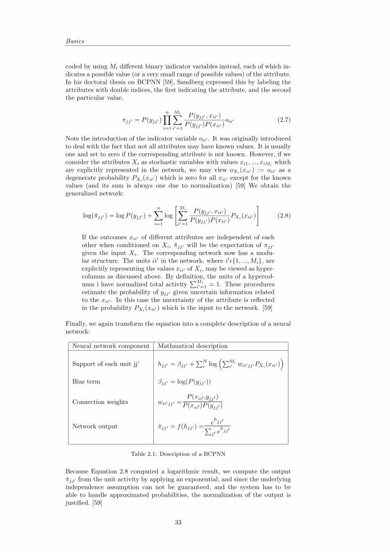
Basics
coded by using Mi different binary indicator variables instead, each of which in-dicates a possible value (or a very small range of possible values) of the attribute.In his doctoral thesis on BCPNN [59], Sandberg expressed this by labeling theattributes with double indices, the first indicating the attribute, and the secondthe particular value.
πjj′ = P (yjj′)
n∏i=1
Mi∑i′=1
P (yjj′ , xii′)
P (yjj′)P (xii′)oii′ (2.7)
Note the introduction of the indicator variable oii′ . It was originally introducedto deal with the fact that not all attributes may have known values. It is usuallyone and set to zero if the corresponding attribute is not known. However, if weconsider the attributes Xi as stochastic variables with values xi1, ..., xiMi
whichare explicitly represented in the network, we may view oXi(xii′) := oii′ as adegenerate probability PXi(xii′) which is zero for all xii′ except for the knownvalues (and its sum is always one due to normalization) [59] We obtain thegeneralized network:
log(πjj′) = logP (yjj′) +
n∑i=1
log
[Mi∑i′=1
P (yjj′ , xii′)
P (yjj′)P (xii′)PXi
(xii′)
](2.8)
If the outcomes xii′ of different attributes are independent of eachother when conditioned on Xi, πjj′ will be the expectation of πjj′
given the input Xi. The corresponding network now has a modu-lar structure. The units ii′ in the network, where i′ε{1, ...,Mi}, areexplicitly representing the values xii′ of Xi, may be viewed as hyper-columns as discussed above. By definition, the units of a hypercol-umn i have normalized total activity
∑Mi
i′=1 = 1. These proceduresestimate the probability of yjj′ given uncertain information relatedto the xii′ . In this case the uncertainty of the attribute is reflectedin the probability PXi(xii′) which is the input to the network. [59]
Finally, we again transform the equation into a complete description of a neuralnetwork:
Neural network component Mathmatical description
Support of each unit jj’ hjj′ = βjj′ +∑Ni log
(∑Mi
i′ wii′jj′PXi(xii′)
)Bias term βjj′ = log(P (yjj′))
Connection weights wii′jj′ =P (xii′ ,yjj′)
P (xii′)P (yjj′)
Network output πjj′ = f(hjj′) =ehjj′∑j′ e
hjj′
Table 2.1: Description of a BCPNN
Because Equation 2.8 computed a logarithmic result, we compute the outputπjj′ from the unit activity by applying an exponential, and since the underlyingindependence assumption can not be guaranteed, and the system has to beable to handle approximated probabilities, the normalization of the output isjustified. [59]
33

Bayesian Confidence Propagation Neural Network (BCPNN)
2.6.4 Recurrent BCPNN
In this latest form (see Table 2.1), the BCPNN takes probability density func-tions as its input and generates probability density functions as its output.Because of this, the network can be used in a recurrent fashion, taking the out-put as the input each next iteration. If the weights and bias are set in a fashioncorresponding to the prior unit-activation probabilities and joint unit-activationprobabilities in a set of input patterns, then the network will converge withina couple of iterations from any other input toward the most probable patternreflected in the weights and bias. These attractor dynamics are obviously quitesimilar to other recurrent neural networks, such as the Hopfield Network.
The BCPNN-Equation for the continuous case can be expressed as:
τcdhjj′(t)
dt= βjj′ +
N∑i
log
(Mi∑i′
wii′jj′f(hii′(t))
)− hjj(t) (2.9)
The time-constant τc can be viewed as a membrane time-constant. It could alsobe tuned to change the speed of the system. Due to the difficulty of computinganalytical solutions for a system this complex (keep in mind that both theweights and bias might change over time due to a not yet specified learningrule), it is useful to discretize time with reasonably small timesteps and executea step by step calculation in any simulation of the network. The system speed isreflected in the size of the time-step (how many recurrent iterations are executedin a given time-interval)
hjj′(t+ 1) = βjj′ +
N∑i
log
(Mi∑i′
wii′jj′f(hii′(t))
)(2.10)
2.6.5 Learning and Forgetting
We now have a functional network architecture. Yet, it remains to be shown howthe network is supposed to learn. We know that weights and bias are conditionedon the probabilities P (xii′) and P (xii′jj′). If all patterns are known in advance,it is obviously possible to count the occurrences and co-occurrences of unitactivations throughout those patterns and then set the probabilities accordingto the statistical counts, which will indeed result in a network with all the desiredattractors (given that the capacity of the net is not exceeded). However, thisscenario is quite unlikely. Any advanced memory system is supposed to be ableto store new information whenever it comes up. We need to build estimatesof said probabilities that reflect the input. In search of a learning-mechanism,Sandberg [59] defined three criteria for picking a solution.
What we aim for is an estimate with the following properties:
• Is should converge toward P (xii′)(t) and P (xii′ , xjj′)(t) in astationary environment.
• It should give more weight to recent than remote information. 24
• It should smooth or filter out noise and adapt to longer trends,in other words lower frequency components of a non-stationaryenvironment.
[59, p.48]
24Note, that this also means, that the system will be capable of dynamic forgetting (avoidingCF), since older information is gradually devalued
34

Basics
The technique of exponential smoothing fulfills all these requirements and byimplementing a discretized time version of exponentially smoothed running av-erages (denoted Λ) with length τL, we obtain the following four-step descriptionof a BCPNN, including the now discrete update and learning rules and a fewother changes:
2.6.6 A Discrete BCPNN Model
Ia. Correcting the current rate estimate of unit ii′:
Λii′(t) = Λii′(t− 1) +1
τL[πii′(t)− Λii′(t− 1)] (2.11)
Ib. Correcting the current rate estimate of connection unit jj′ to ii′:
Λii′jj′(t) = Λii′jj′(t− 1) +1
τL[πii′(t)πjj′(t)− Λii′jj′(t− 1)] (2.12)
II. Bias and Weight Update according to the new probability estimates:
βii′(t) = log(Λii′(t)) (2.13)
wii′jj′(t) =(1− λ20)Λii′jj′(t) + λ20
[(1− λ0)Λii′(t) + λ0][(1− λ0)Λjj′(t) + λ0](2.14)
III. Executing the recurrent unit update, based on new weights and bias:
hii′(t+ 1) = βii′(t) +
N∑i
log
(Mi∑i′
wii′jj′(t)πii′(t))
)(2.15)
IV. Generating the new output from the updated unit support:
πii′(t+ 1) =ehii′ (t+1)∑j′ e
hii′ (t+1)(2.16)
Note that in Equations 2.11 and 2.12, the current estimation error is fed backproportionally with a factor 1
τL, so the inverse of τL can also be interpreted as
a learning-rate αL. Additionally, the careful reader might have noticed that weintroduced constraints to the weight-calculation (Equation 2.14). A minimumactivity λ0 << 1 is introduced, a very small noisy background activity evenlydistributed over all units, overriding probability estimations in the weight cal-culations. This serves to avoid underruns: In the absence of input, the weightswill now converge to 1, so the logarithmic weight converges to zero, correspond-ing to uncoupled units. At the same time, it provides an upper bound on theweight of 1
λ0, avoiding unnecessary windup that might decrease performance for
non-stationary environments.
For a detailed and comparative study of the dynamics of BCPNN, I would like torecommend the work Anders Lansner and Anders Sandberg at the Departmentof Numerical Analysis and Computing Science, Royal Institute of Technology,Stockholm. Specifically the doctoral dissertation of Anders Sandberg [59]
Before we can detail the memory systems approach taken by this thesis, we needto explain yet another augmentation of this BCPNN.
35
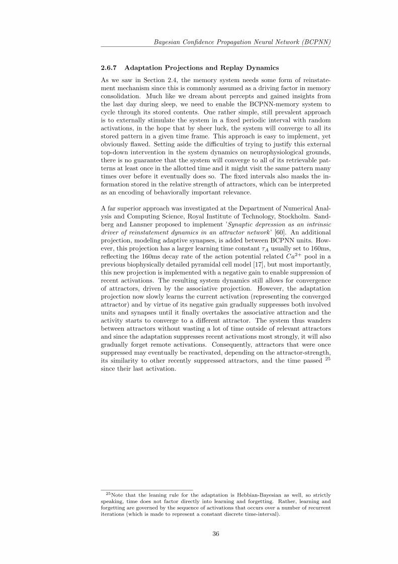
Bayesian Confidence Propagation Neural Network (BCPNN)
2.6.7 Adaptation Projections and Replay Dynamics
As we saw in Section 2.4, the memory system needs some form of reinstate-ment mechanism since this is commonly assumed as a driving factor in memoryconsolidation. Much like we dream about percepts and gained insights fromthe last day during sleep, we need to enable the BCPNN-memory system tocycle through its stored contents. One rather simple, still prevalent approachis to externally stimulate the system in a fixed periodic interval with randomactivations, in the hope that by sheer luck, the system will converge to all itsstored pattern in a given time frame. This approach is easy to implement, yetobviously flawed. Setting aside the difficulties of trying to justify this externaltop-down intervention in the system dynamics on neurophysiological grounds,there is no guarantee that the system will converge to all of its retrievable pat-terns at least once in the allotted time and it might visit the same pattern manytimes over before it eventually does so. The fixed intervals also masks the in-formation stored in the relative strength of attractors, which can be interpretedas an encoding of behaviorally important relevance.
A far superior approach was investigated at the Department of Numerical Anal-ysis and Computing Science, Royal Institute of Technology, Stockholm. Sand-berg and Lansner proposed to implement ’Synaptic depression as an intrinsicdriver of reinstatement dynamics in an attractor network ’ [60]. An additionalprojection, modeling adaptive synapses, is added between BCPNN units. How-ever, this projection has a larger learning time constant τA usually set to 160ms,reflecting the 160ms decay rate of the action potential related Ca2+ pool in aprevious biophysically detailed pyramidal cell model [17], but most importantly,this new projection is implemented with a negative gain to enable suppression ofrecent activations. The resulting system dynamics still allows for convergenceof attractors, driven by the associative projection. However, the adaptationprojection now slowly learns the current activation (representing the convergedattractor) and by virtue of its negative gain gradually suppresses both involvedunits and synapses until it finally overtakes the associative attraction and theactivity starts to converge to a different attractor. The system thus wandersbetween attractors without wasting a lot of time outside of relevant attractorsand since the adaptation suppresses recent activations most strongly, it will alsogradually forget remote activations. Consequently, attractors that were oncesuppressed may eventually be reactivated, depending on the attractor-strength,its similarity to other recently suppressed attractors, and the time passed 25
since their last activation.
25Note that the leaning rule for the adaptation is Hebbian-Bayesian as well, so strictlyspeaking, time does not factor directly into learning and forgetting. Rather, learning andforgetting are governed by the sequence of activations that occurs over a number of recurrentiterations (which is made to represent a constant discrete time-interval).
36

Basics
2.6.8 Final BCPNN-Equation
hii′(t+ 1) =gL
[βii′(t) +
N∑i
log
(Mi∑i′
wii′jj′(t)πii′(t)
)]
+gA
[γii′(t) +
N∑i
log
(Mi∑i′
vii′jj′(t)πii′(t)
)]
πii′(t) =ehii′ (t)∑j′ e
hii′ (t)
Obviously, the adaptation bias and adaptation weights, simulating some sort ofneural (unit) depression and synaptic (weight) depression, need to be learnedas well. The exact same Hebbian-Bayesian learning rule applied to the originalassociative projection can be used for the adaptation projection as well, withthe important distinction that the adaptation works on a different time-scale,governed by τA.
Λii′(t) = Λii′(t− 1) +1
τL[πii′(t)− Λii′(t− 1)] (2.17)
µii′(t) = µii′(t− 1) +1
τA[πii′(t)− µii′(t− 1)] (2.18)
Λii′jj′(t) = Λii′jj′(t− 1) +1
τL[πii′(t)πjj′(t)− Λii′jj′(t− 1)] (2.19)
µii′jj′(t) = µii′jj′(t− 1) +1
τA[πii′(t)πjj′(t)− µii′jj′(t− 1)] (2.20)
βii′(t) = log(Λii′(t)) (2.21)
γii′(t) = log(µii′(t)) (2.22)
wii′jj′(t) =(1− λ20)Λii′jj′(t) + λ20
[(1− λ0)Λii′(t) + λ0][(1− λ0)Λjj′(t) + λ0](2.23)
vii′jj′(t) =(1− λ20)µii′jj′(t) + λ20
[(1− λ0)µii′(t) + λ0][(1− λ0)µjj′(t) + λ0](2.24)
37

Bayesian Confidence Propagation Neural Network (BCPNN)
38

Model and Method
3 Model and Method
3.1 Conceptual Architecture - three-stage-memory
Where does a stable cortical long-term memory engram come from? One way toargue about this, is to say that it is a multi-stage process that starts with sen-sory input to the short-term memory/working memory in the prefrontal cortex(PFC), temporarily involves the hippocampus(MTL) during memory consolida-tion and ends in MTL-independent cortical Long-Term-Memory, from where itcan be retrieved for a long time [39]. The memory system simulated and ana-lyzed in this thesis consists of three populations of BCPNN Units with differentsize, governed by different learning time constants (see Figure 3.1).
PFC 60 Units = 6 Hypercolumns
PFC60 Unitsτ =5ms
MTL120 Unitsτ =300ms
CTX240 Units
τ =18.000ms
Association
Adaptation
Association
Adaptation
PFC2MTL
Hyp
erco
lum
n
Hyp
erco
lum
n
Hyp
erco
lum
n
Hyp
erco
lum
n
Hyp
erco
lum
n
Hyp
erco
lum
n
1 H
yper
colu
mn
= 1
0 M
inic
olu
mn
s
0.01
0.10
0.60
0.05
0.02
0.01
0.01
0.15
0.03
0.02
MTL2CTX
Probability Distribution
Association
Figure 3.1: The three-stage-memory model: From prefrontal sensory memory to longterm cortical memory. To show the probabilistic underpinnings of the BCPNN ar-chitecture, the PFC of 60 BCPNN units is shown to model 6 Hypercolumns. EachHypercolumn consists of 10 minicoumns (so each BCPNN unit models a minicolumn)and together, these 10 minicolumns code for a probability distribution of an attributevalue.
• The first BCPNN-population modeling the PFC has the smallest size (60units) and thus the smallest capacity, but it features the fastest learningwith a time-constant τPFCL = 5 ms. The purpose being, to mimic biolog-ical STM: A rapid memory system, capable of learning even from a singlelearning example, but forgetting equally fast, resulting in highly limitedcapacity.
• The second BCPNN-population modeling the MTL memory system istwice as large and 60 times slower learning with time-constant τMTL
L =300 ms. This system is very similar to BCPNNs analysed by Lansner [31],Sandberg [59] and Liljencrantz [34].
• The last BCPNN-population for modeling LTM in the cortex, doublesthe unit count again (240 units) and slows the learning by another factorof 60: τCTXL = 18.000 ms. The cortex simulation is thus 3600 times
39

Conceptual Architecture - three-stage-memory
slower learning than the PFC simulation. These parameters ensure thatthe cortex mimics LTM properties: Very slow learning and forgettingand a relatively large capacity. It is obviously hard to teach a memorysystem this slow anything without serious efforts of learning repetitionand reinstatement dynamics.
In further discussion, we sometimes refer to the hierarchy PFC-MTL-CTX as ahierarchy of memory stages, with PFC at the first stage, and cortex as the laststage of the overall memory system.
3.1.1 Activation Patterns
All three networks make use of a columnar organization with ten units perhypercolumn. Due to the probabilistic underpinning of BCPNNs, each unitmodeling a minicolumn takes a value between zero and one and the total acti-vation within each hypercolumn is normalized to one, corresponding to a totalneural activity level of 10% in each network.
Learning examples shown to the system throughout various simulations, can beexpressed in a somewhat shorter form as decimal strings with a length corre-sponding to the number of hypercolumns. The reason for this is quite simply,that learning examples by definition do not have a lot of uncertainty, so theyhave only one fully activated unit per hypercolumn. In a straight forward ap-proach, each hypercolumn is assigned a value between zero to nine, shorteningthe representation of each hypercolumns activation to one decimal digit. Thepatterns are activated with some additional low level noise on all units but over-all, the confidence distributions are unambiguous and can be represented by thenumber of the activated unit instead. This approach can achieve somewhatdecorrelated 26 learning patterns. This is justified on three accounts:
• First, there is clear evidence that memories are decorrelated by lower ordernetworks before storage [76, and references therein].
• Second, this approach is representative of selective neurological columns(see Section 2.3.1).
• Third, the simulation is bound by computational limits to use artificiallylow dimensionality of input patterns. Compensating for the decreasedorthogonality of patterns to some extent is reasonable. Especially sinceno decorrelation pre-filter is used and no selection or ordering of patternsbesides random permutation is implemented.
Example: A PFC pattern ξ =’219842’ Denotes a clear activation ofunits x2, x11, x29, x38, x44, x52 with some low-level noise on all otherPFC units. The total activity is six, which is an activity level of10%.
All learning patterns are generated randomly under these rules. It is easy tosee that this means a million possible PFC patterns, a trillion possible MTLpatterns, and a septillion possible cortical patterns. We note, the resulting pat-terns are still correlated to some extent even if we do not account for distributednoise. (e.g. Given any random MTL pattern, 70% of all other MTL patternsshare at least one unit activation with that pattern.)
26Obviously patterns will become more orthogonal/decorrelated in BCPNNs of higher di-mensionality, i.e. networks with more columns
40

Model and Method
3.1.2 Adaptations
To enable autonomous training pattern reactivation, both PFC and MTL makeuse of an adaptation projection in line with the mathematical model laid out inSection 2.6.8. Unless stated otherwise, the adaptations run with a learning timeconstant of τPFCA = τMTL
A = 160 ms, reflecting biophysically detailed models(see Section 2.6.7). The adaptation gains are obviously negative and chosen tobe gPFCA = −1.4 and gMTL
A = −1.4.
3.1.3 Plastic Connections
The three memory systems PFC, MTL, and cortex are connected by two con-nections named PFC2MTL and MTL2CTX. There are several possible ways ofsetting up these connections. A previous Master Thesis [34] at the Departmentof Numerical Analysis and Computer Science at the Royal Institute of Tech-nology investigated these and compared several static projections (1-to-1, staticsubset/pattern-prefix, orthogonal subset) against plastic connections. Thereare several benefits to using plastic connections instead of a static scheme forassociating patterns from different BCPNNs with one another:
A static projection from the MTL to cortex did not give acceptableperformance. The best performance when using static projectionswas obtained by using a simple 1-to-1 connection between the MTLand a subset of the cortex, and no other MTL to cortex connections.It seems that when using static MTL to cortex projections, the net-work does not benefit from having a cortex which is larger than theMTL. This can also be seen from the very large performance decreasewith a smaller MTL [...] The performance of the network is muchbetter when using plastic MTL to cortex projections. Depending onthe type of pattern used in the MTL, between 60 and 80% of thenetworks maximum capacity can be reached. The network is robustwith regard to its parameters. [34]
The investigation also led to the conclusion, that the viability of memory con-solidation is critically dependent on the replay performance. We will see, howplastic connections stabilize replay behavior and improve overall performance,while at the same time allowing for complete freedom in the choice of patternsand increased overall memory capacity.For the model of this thesis, plastic connections PFC2MTL and MTL2CTX wereset to learn fast enough to encode the association between patterns on differentstages on first try: τPFC2MTL = τMTL2CTX = 20ms. The high speed obviouslyreduces the capacity of the association, but that is not an unwanted effect. Theassociation only needs to hold long enough for successful consolidation of thecorresponding pattern to occur on the next stage. In fact, over the course ofthe simulation it is entirely possible that the same PFC pattern maps to severaldifferent cortical patterns at different points in time. This does not prevent thesepercepts from being consolidated into the cortex one after another however.
3.1.4 The Simulation Cycle and Timing
We ultimately want to show the consolidation performance of the overall mem-ory system. For that reason, all learning of both MTL and cortex is limitedto learning by consolidation. We cut any direct learning of MTL and cortex(corresponding to vector Sc(O) in the standard model in Figure 2.16) by deac-tivating their learning capability when new patterns are first presented to thesystem. Consolidation is achieved through reactivation of patterns, driven bythe adaptation/replay dynamics of the earlier stages. So strictly speaking, wenot only simulate the MTL as a teacher to the cortex, but we even teach the
41

Conceptual Architecture - three-stage-memory
Reflection800ms
Perception
40ms
Reflection800ms
Perception
40ms
Night 18.000ms
Random patterns
4 new patterns
4 new patterns
Figure 3.2: The simulation cycle
teacher (MTL) first via an adaptation driven PFC replay before it then teachesthe cortex. In this sense, we aim to test the viability of a consolidation-chain(see second objective in Section 1.2).The simulation evolves in phases (see Figure 3.2). We simulate multiple days,which we divide into two parts: night and day. Each day consists of two phasesof perception, during which we feed the PFC with new patterns to be learnedand define associated patterns for the later stages (setting PFC2MTL andMTL2CTX). MTL and cortical weights remain unchanged during this phase.Each perception phase is followed by a reflection phase, during which newlylearned patterns are taught/consolidated into the MTL. Under ideal circum-stances the MTL learned all newly perceived patterns at the end of the day.Finally, during the night phase we allow for the MTL to teach the cortex and/orconsolidate existing cortex patterns.
3.1.5 Simulation-Phase: Perception
In the initialization of the perception phase, we activate the PFC learning bysetting αPFCL = 1
5ms while disabling the adaptation: αPFCA = 0, gPFCA = 0.Both MTL and cortex have their projections disabled and their learning ratesset to zero, effectively silencing all activity in these networks. This cuts anydirect learning during perception and enables us to measure only the subsequentlearning by consolidation.During perception we also associate every new PFC pattern with a correspond-ing MTL and cortex pattern: αPFC2MTL
L = αMTL2CTXL = 1
20msThe perception phase lasts for only 40ms. The timestep is 10ms, so we havetime to train each of the four new patterns only for a single timestep. This isdone by clamping the unit activity to the training pattern, allowing the weightsto adapt. However, since the PFC is fast learning, it is guaranteed to learn allfour new patterns, while potentially erasing older patterns.
3.1.6 Simulation-Phase: Reflection
Following the perception phase, we attempt to learn representations of the newinputs in the MTL. We deactivate learning in the PFC (αPFCL = 0), whileactivating its recurrent and adaptation projection: gPFCL = 1, gPFCA = −1.4,αPFCA = 1
160ms .
This will result in autonomous reactivation of stored PFC patterns, which willin turn cause the corresponding MTL patterns to be projected and we activatelearning in the MTL to have the MTL taught through the reinstatement dy-namics of the PFC: αMTL
L = 1300ms . The reflection phase is 20 times longer
than the perception phase and lasts for 800ms.
42

Model and Method
10 ms forcedactivation per
pattern
PFC60 Unitsτ =5ms
MTL120 Units
τ = ∞
CTX240 Units
τ = ∞
Association
Adaptation
Association
Adaptation
PFC2MTL MTL2CTX
Association
Perception Phase (40ms)
PFC60 Unitsτ =5ms
MTL120 Unitsτ =300ms
CTX240 Units
τ =∞
Association
Adaptation (160ms)
Association
Adaptation
PFC2MTL MTL2CTX
Association
Reflection Phase (800ms)
PFC60 Units
τ =∞
MTL120 Unitsτ =300ms
CTX240 Units
τ =18.000ms
Association
Adaptation
Association
Adaptation (160ms)
PFC2MTL MTL2CTX
Association
Night Phase (16.000ms)
Input:Forced
Activation
Input:Forced
Activation
4 Random patterns
Input:
Set upplastic
connections
Set upplastic
connections
Figure 3.3: The three simulation phases and their active components
3.1.7 Simulation-Phase: Night
Following two perception-reflection cycles during the day, we start the nightphase by deactivating all PFC projections. This reflects the inactivity of sensoryareas during sleep. We now hope to store representations of the new patternsin the cortex as well as to further the ongoing consolidation of older patterns,already stored (but weakly so) in the cortex.
We deactivate learning in the MTL (αMTLL = 0), whilst activating its recurrent
and adaptation projection: gMTLL = 1, gMTL
A = −1.4, αMTLA = 1
160ms .
This will result in autonomous reactivation of stored MTL patterns (both fromthis day as well as remaining older ones), which will in turn cause the corre-sponding cortex-patterns to be projected and we activate learning in the cortexduring the night, to have the cortex taught through the reinstatement dynamicsof the MTL: αCTXL = 1
18s . The night phase is 20 times longer than the reflectionphase and lasts for 16s.
43

Model Parameters
3.2 Model Parameters
A general overview over the model parameters, such as time-constants and im-portant gains, can be found in Table 3.1.
PFC MTL CTXBCPNN Units NPFC 60 NMTL 120 NCTX 240Association gain gPFCL +1 gMTL
L +1 gCTXL +1Adaptation gain gPFCA -1.4 gMTL
A -1.4Association time-constant τPFCL 5 ms τMTL
L 300 ms τCTXL 18sAdaptation time-constant τPFCA 160 ms τMTL
A 160 ms
Time discretization dt 10msPhase duration Tperception 40msPhase duration Treflection 800msPhase duration Tnight 16000msWeight estimation noise λ0 = dt
τMTLA
6.25%
Table 3.1: General overview of the simulation model parameters
3.3 Retrieval Testing
Evaluation of pattern storage is based on successful retrieval. To test retrievalof a training pattern ξp on a specific memory stage, learning is deactivatedand the network is cued with the training pattern that, however, had threerandomly chosen hypercolumn activations interchanged first.27 The network isthen allowed to associate freely, while the resulting change in activity is mea-sured by ∆π(t) = |π(t− dt)− π(t)|. As long as the change is significantly large,the network is considered to still converge and allowed to associate for anothertime step. Once the activity change drops below a defined threshold, the over-
lap O(ξp, π(t)) = ξp·π(t)|ξp||π| is measured. The training pattern is then considered
successfully retrieved, if this overlap is larger than 95%.Since the patterns are stochastic, as is the resulting system behavior, we in-troduce the retrieval rate ρ, which simply states the odds of successful patternretrieval. As we can test retrieval for different parts of the system we specifyρPFC , ρMTL, and ρCTX to express the retrieval rates with respect to a specificmemory stage. In certain cases, we are not interested to look at the retrievalrate of a specific memory subsystem, rather, we want to know whether a patternis stored in any of the three networks. We thus also introduce a general retrievalrate ρPMC , which indicated the retrieval rate of the combined network. For anysingle simulation ρPMC is computed from logically OR-connecting the patternretrieval from all three networks, which results in ρPMC = 1 when the specificpattern can be retrieved from at least one network and ρPMC = 0 otherwise.ρPMC consequently does not provide any indication of storage redundancy.
3.4 Criteria for Evaluating Replay Performance
What do we mean by replay performance?
• Variety: We hope to cycle through as many stored patterns as possibleand activate them many times over.
• Strength: We hope to activate these patterns as clearly as possible(strong overlap of activation and a training pattern).
27In PFC testing, only two hypercolumns of the training pattern are scrambled, becauseotherwise, this approach become unproportionally harsh for PFC testing where the networkhas only six hypercolumns after all and the likelihood of accidentally testing a different trainingpattern is not insignificant.
44
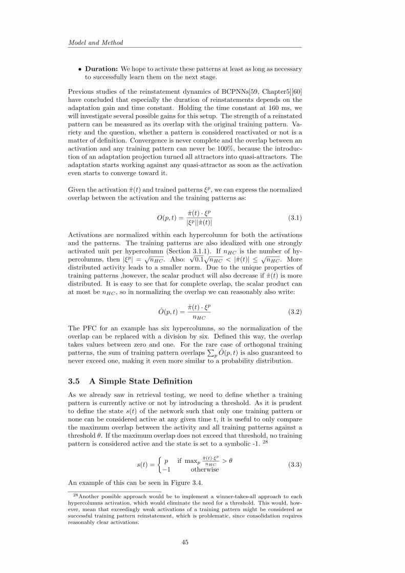
Model and Method
• Duration: We hope to activate these patterns at least as long as necessaryto successfully learn them on the next stage.
Previous studies of the reinstatement dynamics of BCPNNs[59, Chapter5][60]have concluded that especially the duration of reinstatements depends on theadaptation gain and time constant. Holding the time constant at 160 ms, wewill investigate several possible gains for this setup. The strength of a reinstatedpattern can be measured as its overlap with the original training pattern. Va-riety and the question, whether a pattern is considered reactivated or not is amatter of definition. Convergence is never complete and the overlap between anactivation and any training pattern can never be 100%, because the introduc-tion of an adaptation projection turned all attractors into quasi-attractors. Theadaptation starts working against any quasi-attractor as soon as the activationeven starts to converge toward it.
Given the activation π(t) and trained patterns ξp, we can express the normalizedoverlap between the activation and the training patterns as:
O(p, t) =π(t) · ξp
|ξp||π(t)|(3.1)
Activations are normalized within each hypercolumn for both the activationsand the patterns. The training patterns are also idealized with one stronglyactivated unit per hypercolumn (Section 3.1.1). If nHC is the number of hy-percolumns, then |ξp| =
√nHC . Also:
√0.1√nHC < |π(t)| ≤ √nHC . More
distributed activity leads to a smaller norm. Due to the unique properties oftraining patterns ,however, the scalar product will also decrease if π(t) is moredistributed. It is easy to see that for complete overlap, the scalar product canat most be nHC , so in normalizing the overlap we can reasonably also write:
O(p, t) =π(t) · ξp
nHC(3.2)
The PFC for an example has six hypercolumns, so the normalization of theoverlap can be replaced with a division by six. Defined this way, the overlaptakes values between zero and one. For the rare case of orthogonal trainingpatterns, the sum of training pattern overlaps
∑p O(p, t) is also guaranteed to
never exceed one, making it even more similar to a probability distribution.
3.5 A Simple State Definition
As we already saw in retrieval testing, we need to define whether a trainingpattern is currently active or not by introducing a threshold. As it is prudentto define the state s(t) of the network such that only one training pattern ornone can be considered active at any given time t, it is useful to only comparethe maximum overlap between the activity and all training patterns against athreshold θ. If the maximum overlap does not exceed that threshold, no trainingpattern is considered active and the state is set to a symbolic -1. 28
s(t) =
{p if maxp
π(t)·ξpnHC
> θ
−1 otherwise(3.3)
An example of this can be seen in Figure 3.4.
28Another possible approach would be to implement a winner-takes-all approach to eachhypercolumns activation, which would eliminate the need for a threshold. This would, how-ever, mean that exceedingly weak activations of a training pattern might be considered assuccessful training pattern reinstatement, which is problematic, since consolidation requiresreasonably clear activations.
45

Quantifying Replay Performance Criteria
5 10 15 200
0.1
0.2
0.3
0.4
0.5
0.6
0.7
0.8
0.9
1
Training Pattern
Ove
rlap
5 10 15 200
0.1
0.2
0.3
0.4
0.5
0.6
0.7
0.8
0.9
1
Training Pattern
Ove
rlap
Figure 3.4: Overlaps for two activations were computed according to Equation 3.2.At θ = 0.85, the state for the left plot is s = 15, while the state for the right plot isdefined as unknown, s = −1, because the activation of training pattern ξ18 is deemedinsufficient.
3.6 Quantifying Replay Performance Criteria
With the new state definition (Equation 3.3), we finally acquired the means toquantify the three criteria laid out for evaluation replay performance: Variety,Strength, and Duration.
One way of quantifying the variety during replay is to count the number oftimes, a pattern becomes active according to the state definition. If we recordthis count for all training patterns/possible states, we gain insight into thevariety during replay.
The parameter NPR, denotes the number of pattern activationsduring replay, as measured by the state definition in Equation 3.3.
The strength of an activation can be captured by the overlap as defined in Equa-tion 3.2. To quantify the duration of reinstatements, we can also record howlong a pattern remains active according to the state definition in Equation 3.3.This is naturally a stochastically varying property, as reinstatements can bedifferent in length, depending on how quickly they become suppressed by theadaptation projection. Instead of simply computing a mean activation time 29,we could also show the reinstatement length distribution for each pattern/state.
The parameter RLD denotes the reinstatement length distribution,which shows the heuristic probability of a certain reinstatementlength for a given pattern.
Often times it is interesting to combine NPR and RLD into a measurement oftotal pattern reinstatement length, to know how long a specific state has beenactive in total, so we finally introduce a third parameter.
The parameter TPRL denotes the total pattern reinstatement length,which is recorded by summing up the length of all reinstatements ofa pattern during the entire replay period.
Naturally TPRL increases with both the number of activations as well as thelength of the reinstatements following each activation.
29This is sometimes referred to as average dwell time in other papers.
46

Model and Method
3.7 Simulated Hippocampal Lesioning
In order to simulate hippocampal lesioning, we disconnect units within theBCPNN used for modeling the MTL/hippocampus. The mathematical BCPNNframework (see Section 2.6.8) uses logarithmic weights for expressing the con-nectivity between units. We can artificially disconnect units ii’ and jj’ by settingweight wMTL
ii′jj′ = 1, as the log weight will then approach zero and thus expressneither excitatory nor inhibitory connectivity.
For implementing varying degrees of hippocampal lesioning, we define a damageratio χ, which expresses the ratio of nullified weights to the overall number ofconnection weights. To avoid any bias against specific training patterns, theconnection weights to be nullified are drawn randomly from all possible weightsuntil the set damage defined by ratio χ has been achieved.
To obtain a measurement of retrograde amnesia, we first run a full simula-tion and then test regular memory retrieval before implementing simulated hip-pocampal lesioning and retesting the memory retrieval afterwards. As patternsmay be retrieved from either PFC, MTL or cortex and we may not want todistinguish the origin of a retrieved pattern in quantifying amnesia 30, we alsouse the retrieval rate ρPMC , which indicates retrieval from any stage.For quantifying anterograde amnesia we then attempt to use a damaged systemfor memory consolidation by running a regular simulation and observing howmany patterns can still be consolidated into MTL and cortex despite the nullifiedweights, and how the overall retrieval rate ρPMC changes when compared to anundamaged system.
3.8 Runtime Environment
The entire model was developed and run under MATLAB. The functionalityis modularized, scalable, and all simulation parameters set in a separate ini-tialization step to allow for maximum flexibility and future development. Thisapproach provides optimal debugging capability and program variability whilesacrificing a lot of speed compared to say a C++ compiled executable. Thisis partially compensated by making full use of MATLABs strengths in dealingwith matrices, so some effort was spent on vectorizing the program and express-ing as many program steps as possible as matrix computations, while avoidingslow loops.
3.9 Performance of Subsystems and Experimental Expec-tations
In this section, we take a look at the performance, capabilities, and sensitivitiesof individual subsystems of the overall model, to get a better understanding ofthe model behavior and abstract some reasonable predictions for the full scalesimulation.
3.9.1 PFC: Capacity and Replay Performance
The PFC simulation exhibits one shot learning due to its fast learning capability.In the following preliminary investigation, each training pattern, ξ1 to ξ20, isshown to the network for only one iteration (10 ms each). After this initialtraining, retrieval is tested as described in Section 3.3. We can see (Figure 3.5),
30In fact, we can not tell by conscious experience, where we retrieve our memories from.Whether a memory is still dependent on the hippocampus or already fully consolidated intohippocampus-independent LTM is not revealed to us upon conscious recollection or introspec-tion.
47
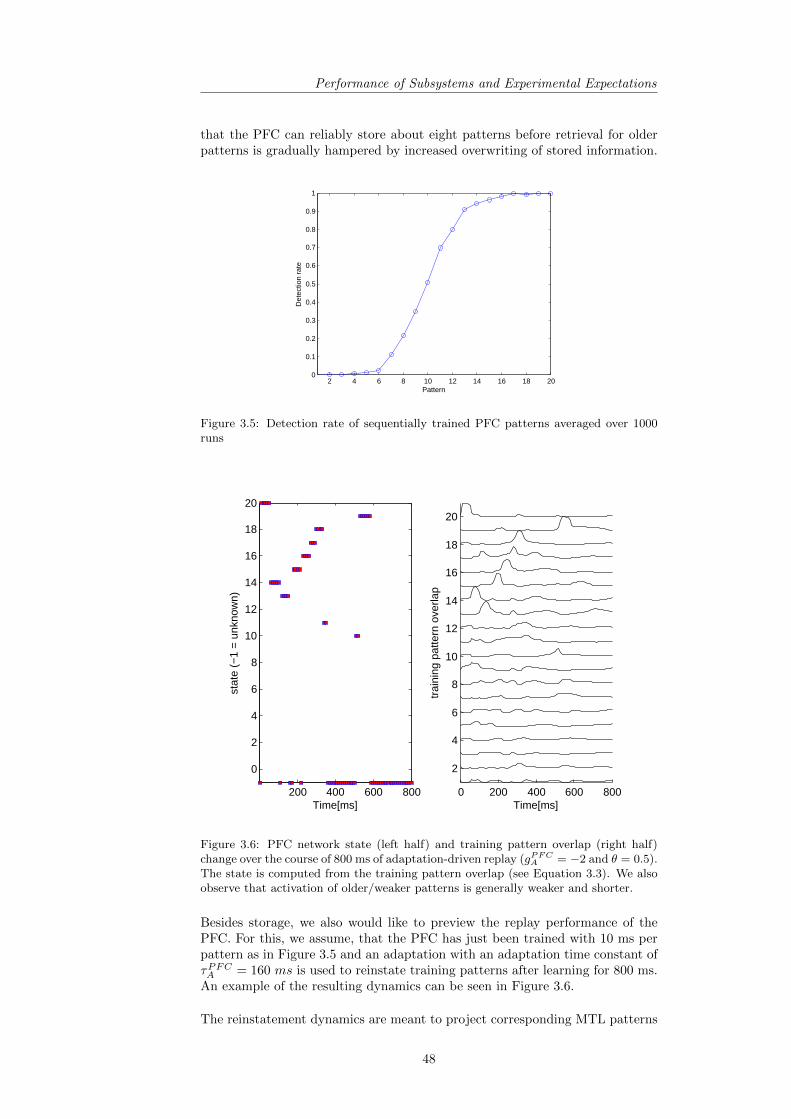
Performance of Subsystems and Experimental Expectations
that the PFC can reliably store about eight patterns before retrieval for olderpatterns is gradually hampered by increased overwriting of stored information.
2 4 6 8 10 12 14 16 18 200
0.1
0.2
0.3
0.4
0.5
0.6
0.7
0.8
0.9
1
Pattern
Det
ectio
n ra
te
Figure 3.5: Detection rate of sequentially trained PFC patterns averaged over 1000runs
200 400 600 800
0
2
4
6
8
10
12
14
16
18
20
stat
e (−
1 =
unk
now
n)
Time[ms]0 200 400 600 800
2
4
6
8
10
12
14
16
18
20
Time[ms]
trai
ning
pat
tern
ove
rlap
Figure 3.6: PFC network state (left half) and training pattern overlap (right half)change over the course of 800 ms of adaptation-driven replay (gPFC
A = −2 and θ = 0.5).The state is computed from the training pattern overlap (see Equation 3.3). We alsoobserve that activation of older/weaker patterns is generally weaker and shorter.
Besides storage, we also would like to preview the replay performance of thePFC. For this, we assume, that the PFC has just been trained with 10 ms perpattern as in Figure 3.5 and an adaptation with an adaptation time constant ofτPFCA = 160 ms is used to reinstate training patterns after learning for 800 ms.An example of the resulting dynamics can be seen in Figure 3.6.
The reinstatement dynamics are meant to project corresponding MTL patterns
48

Model and Method
to be activated in the MTL via the PFC2MTL connection31. We now show thetotal time spent near the MTL patterns ξ1 to ξ20, for different detection thresh-olds and adaptation gains in Figure 3.7. Note, that we now apply Equations 3.2and 3.3 on the MTL, despite the fact that the network dynamics are driven byPFC replay.
5 10 15 200
100
200
5 10 15 200
100
200
5 10 15 200
100
200
5 10 15 200
100
200
5 10 15 200
100
200
MTL Pattern5 10 15 20
0
100
200
MTL Pattern
θ =0.85θ = 0.5
gA=−2
gA=−1.5
gA=−1
Figure 3.7: Total time spent near (O(p, t) > θ) different MTL patterns during PFCreplay (in ms) for six scenarios with different gA and θ, each averaged over 1000 runswith random PFC and MTL training patterns.
Consider the following argument: Stronger adaptation gains drive the activityaway from quasi-attractors, that it started to converge to, which leads to morebut shorter periods of convergence and ultimately also less total time spentnear MTL patterns. This effect can be seen across all patterns, but is espe-cially dominant for the last trained pattern ξ20. While it is by far the mostreinstated pattern for an adaptation gain of gA = −1, its presence in the replayperiod quickly diminishes for a more negative gain. This can be seen as wellfor a stricter state definition (right half of Figure 3.7), which generally tends tolower our accounts of perceived reinstatements. Changing θ mostly preservesthe shape of the distribution, indicating that weak reactivations occur amongall pattern reactivations occasionally. For gA = −1 and θ = 0.5 the networkspends 98% of its time near a pattern. For an adaptation gain gA = −2 anda more restrictive definition of ’near’ (θ = 0.85), this drops to less than half ofthe total replay time. We saw earlier, that the PFC can reliably store aboutthe last eight patterns, so it is not surprising that the eight most recent PFCpatterns are reactivated the most, leading to activations of corresponding MTLpattern.
Two observations, however, are indeed surprising and deserves further scrutiny:
• For some reason, the last pattern ξ20 is especially sensitive to changes inthe adaptation gain and moreover dominates replay for weaker adaptationgains, where the system spends unusually long time near that pattern.
• In direct contradiction to arguments made by Lansner and Sandberg[60] [59,p.88] on a similar setup, the strongest pattern (ξ20, because it was trained
31The plastic PFC2MTL connection is already established -learned- on the grounds, thatwe do not wish to model this process of association or choose a static connectivity but ratherassume that arbitrary PFC patterns can be associated with arbitrary MTL patterns
49

Performance of Subsystems and Experimental Expectations
last) is not generally activated the most, neither is second or third strongest,but rather the fifth most recently trained pattern, ξ16.
As to the reasons for anomalies, we may speculate that while all recent patternare basically guaranteed to be visited, the strongest patterns converge more com-pletely at first. This leads to a very strong adaptation, that can not be overcomein the limited time, to reactivate the pattern again or is generally stronger thanthat of weaker patterns, which also activate much more weakly. This view issupported by the observation, that a tighter state definition (choosing a largerθ, to neglect weakly converged attractors) will reduce the local maximum nearξ16. Due to nonlinearities, an analytical approach to this question is not feasi-ble. If we except this first explanation, this still leaves out an explanation theabnormal behavior of the last pattern.There actually exist two separate rather surprising answers to both problems.They have to do with general properties of BCPNN replay and some other pecu-liar aspects of this specific setup. For our general model setting with gA ' 1.5,both problems are not too extreme, but will obviously have an impact on thesystem in later performance. We will investigate these details more closely inresponse to our first major simulation scenario (Sections 4.2 and 5.6), where wedissect the inner dynamics of replay. For now, we leave this preliminary inves-tigation of the PFC with an estimate, that under the current model parameters(gA ' 1.5, τA = 160 ms) and a θ = 0.5 metric, the eight most recent MTLpatterns become reactivated for about 66 ms each.
3.9.2 MTL: Capacity and Replay Performance
For this preliminary investigation, the MTL is presented with 80 patterns whichare trained sequentially. Each pattern is trained for the same time. In Fig-ure 3.8, we can see that in contrast to the PFC, the MTL is not capable ofone-shot learning: No pattern can be retrieved after training each pattern for10 ms (one iteration). By increasing the training time to 50 ms for each pattern,we can reliably retrieve about the last 25 patterns, depending on how certainwe need to be. The odds of successful retrieval for the last trained patterns canbe increased even further, by further lengthening the training time, but at thecost of drastically reducing the overall capacity.
0 10 20 30 40 50 60 70 800
0.1
0.2
0.3
0.4
0.5
0.6
0.7
0.8
0.9
1
Pattern
Det
ectio
n ra
te
10ms20ms50ms100ms400ms
Figure 3.8: Detection rate of sequentially trained MTL patterns ξ1 to ξ80 averagedover 1000 runs
Increasing the training time also has an effect on the speed of convergence inmemory retrieval. In Figure 3.9, we can see the overlap between the training
50

Model and Method
pattern to be retrieved and the network activation after one iteration (10 ms) ofretrieval testing. Longer training time leads to faster convergence of the trainedpattern for recently trained patterns (closer to 100% overlap after the first itera-tion). At the same time, retrieval of older patterns becomes slower. Retrieval istested by cued recall with a cue similar to the training pattern. For MTL test-ing, 9 out of 12 hypercolumns are identical to the training pattern, leading to atleast 75% overlap at the start of retrieval testing, so further decreasing overlappoints at the fact, that the network converges to other quasi-attractors/patternsinstead.
0 10 20 30 40 50 60 70 800.1
0.2
0.3
0.4
0.5
0.6
0.7
0.8
0.9
1
Pattern
Mea
n ov
erla
p af
ter
first
iter
atio
n
10ms20ms50ms100ms400ms
Figure 3.9: Mean overlap after one iteration of pattern retrieval averaged over 1000runs
Similar to our investigation of the PFC replay, we now use the trained MTL (80patterns trained directly) and activate its adaptation projection for 16.000 ms,which corresponds to the length of the planned night phase. Besides the pos-sibility of tuning gMTL
A = −1.4, we are most interested in how sensitive thereplay performance is to the strength of the taught quasi-attractors, which isdirectly related to the amount of time that was spent on training them. Con-trary to the PFC, however, there is no fixed training time for MTL Patterns.The strength of an MTL encoding depends on the PFC replay performance andhow many other patterns were taught after it (potentially overwriting some ofthe encoding).
It should not go unmentioned here, that the total pattern reactivation length(TPRL) is much more in line with the idea, that the strength of initial encodingand replay performance should be highly correlated. Given that the networkparameters are time-invariant and the training-time for each training patternis constant as well, the position of a pattern directly relates to its encodingstrength. The plots in Figure 3.10 agree with this notion. None of the contra-dictions and surprises, that we previously found in the PFC replay dynamicscan be seen here.
3.9.3 CTX: Learning and Capacity
The cortex simulation learns excessively slow. Figure 3.11 underscores that fact.Presenting each training pattern for 250 ms yields no retrieval at all. We needto increase exposure to 1000 ms before we can reliably retrieve about the last 56training patterns. Quadrupling the learning time to 4000 ms per pattern yieldsstronger encoding (see Figure 3.12) in exchange for only a decrease of capacityto about 40 reliably retrievable patterns.
51

Consolidation Expectations
50 60 70 800
50
100
150
200
250
300
350
400
450
500
TMTLencode
=50ms
Pattern
tota
l tim
e sp
end
near
( θ
= 0
.5 )
eac
h C
TX
Pat
tern
[ms]
50 60 70 800
50
100
150
200
250
300
350
400
450
500
TMTLencode
=75ms
Pattern50 60 70 80
0
50
100
150
200
250
300
350
400
450
500
TMTLencode
=100ms
Pattern
Figure 3.10: Total time spent near (θ = 0.5) different cortical patterns during16.000 ms of MTL replay for three scenarios, where we changed the strength of the ini-tial MTL encoding by varying TMTL
encode, the training time for each pattern. Performancewas averaged over 100 runs with random MTL and CTX training patterns.
0 10 20 30 40 50 60 70 800
0.1
0.2
0.3
0.4
0.5
0.6
0.7
0.8
0.9
1
Pattern
Det
ectio
n ra
te
250ms500ms1000ms2000ms4000ms
Figure 3.11: Detection rate of sequentially trained cortical patterns ξ1 to ξ80 averagedover 100 runs
3.10 Consolidation Expectations
In this section, we use the data from our early investigation of the subsystems ofthe model to logically deduce some rough estimates of what we can reasonablyexpect the whole model to accomplish. We already concluded that the PFCwould be capable of projecting the eight strongest patterns in every reflectioncycle (Figure 3.5). We also know that it takes 50-100 ms to successfully trainthe MTL directly with clear 32 training patterns(Figure 3.8). When learningthrough reinstatement, these patterns are projected somewhat weaker. Usingthe θ = 0.5 metric, we know, that the eight last training patterns will be acti-vated (with at least 50% training pattern overlap) for about 66 ms (Figure 3.7).We introduce eight patterns every day and consolidate twice, so we can expectthe strongest eight patterns in the PFC to be consolidated for about 132 mseach. If learning by projection is on average about 3
4 as efficient (wild guess)as direct training with a clear trainingpattern, then this might be equivalent to
32By ’clear’, we mean a near complete overlap of the activated pattern with the trainingpattern
52
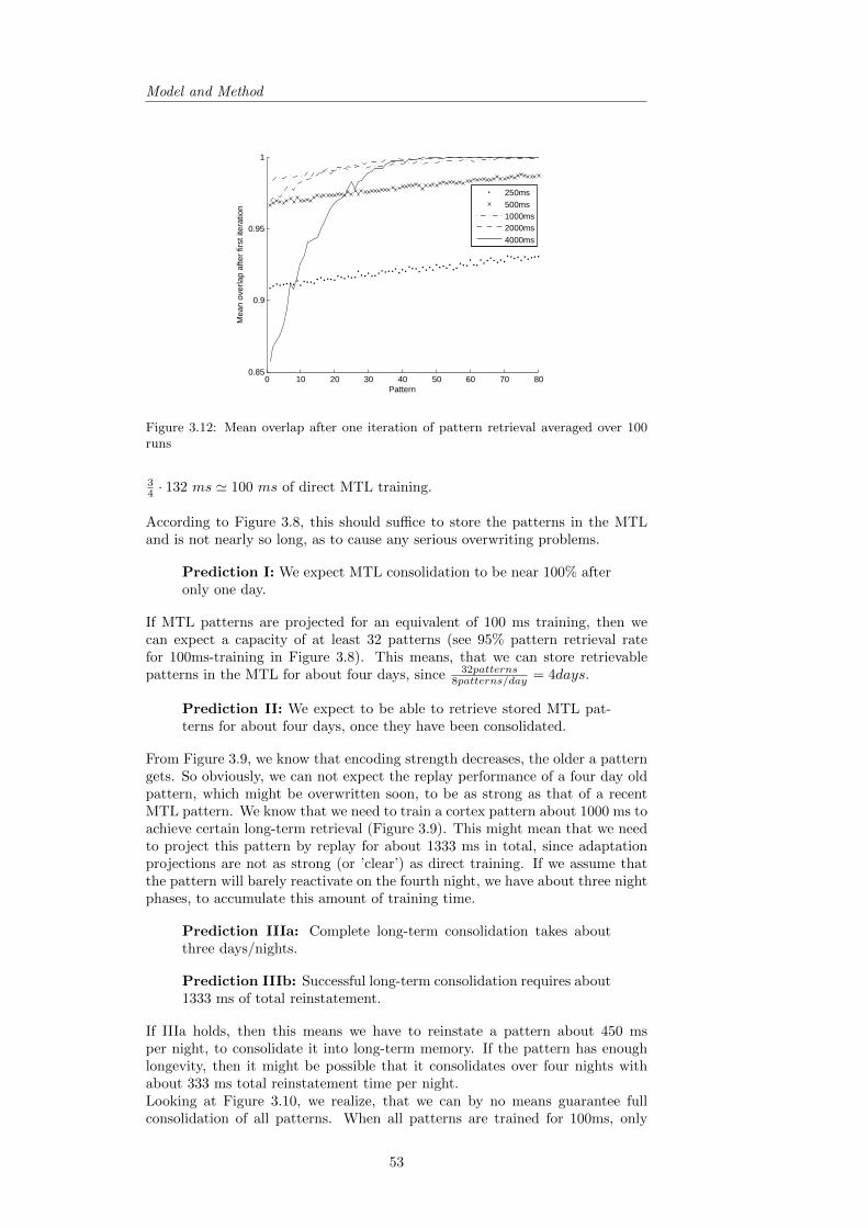
Model and Method
0 10 20 30 40 50 60 70 800.85
0.9
0.95
1
Pattern
Mea
n ov
erla
p af
ter
first
iter
atio
n
250ms500ms1000ms2000ms4000ms
Figure 3.12: Mean overlap after one iteration of pattern retrieval averaged over 100runs
34 · 132 ms ' 100 ms of direct MTL training.
According to Figure 3.8, this should suffice to store the patterns in the MTLand is not nearly so long, as to cause any serious overwriting problems.
Prediction I: We expect MTL consolidation to be near 100% afteronly one day.
If MTL patterns are projected for an equivalent of 100 ms training, then wecan expect a capacity of at least 32 patterns (see 95% pattern retrieval ratefor 100ms-training in Figure 3.8). This means, that we can store retrievablepatterns in the MTL for about four days, since 32patterns
8patterns/day = 4days.
Prediction II: We expect to be able to retrieve stored MTL pat-terns for about four days, once they have been consolidated.
From Figure 3.9, we know that encoding strength decreases, the older a patterngets. So obviously, we can not expect the replay performance of a four day oldpattern, which might be overwritten soon, to be as strong as that of a recentMTL pattern. We know that we need to train a cortex pattern about 1000 ms toachieve certain long-term retrieval (Figure 3.9). This might mean that we needto project this pattern by replay for about 1333 ms in total, since adaptationprojections are not as strong (or ’clear’) as direct training. If we assume thatthe pattern will barely reactivate on the fourth night, we have about three nightphases, to accumulate this amount of training time.
Prediction IIIa: Complete long-term consolidation takes aboutthree days/nights.
Prediction IIIb: Successful long-term consolidation requires about1333 ms of total reinstatement.
If IIIa holds, then this means we have to reinstate a pattern about 450 msper night, to consolidate it into long-term memory. If the pattern has enoughlongevity, then it might be possible that it consolidates over four nights withabout 333 ms total reinstatement time per night.Looking at Figure 3.10, we realize, that we can by no means guarantee fullconsolidation of all patterns. When all patterns are trained for 100ms, only
53
Consolidation Expectations
the eight strongest patterns are projected 450 ms or longer. Under the laidout assumptions, if we wanted to consolidate all patterns into LTM, we wouldneed to project 8patterns/day ·3days = 24patterns with more than 450 ms eachnight. Because we accomplish less than that, we expect the ratio of consolidatedpatterns to be about 8patterns
24patterns = 33%
Prediction IV: We expect roughly 33% of all patterns to be con-solidated into long-term memory.
On the other hand, a low consolidation rate bodes well for the longevity ofcortical patterns. If less than 33% of patterns are consolidated (2-3 per day),then the cortical capacity will last for some patterns to be retained for two tothree weeks, as the reliable capacity for 1000ms-training is about 56 patterns.(Figure 3.11): 56patterns
2.66pattern/day = 21days = 3weeks. One more consideration to
take into account might be the fact that even while we might not store more thantwo to three patterns per day, other failed attempts at consolidating additionalpatterns might inevitably corrode our long-term capacity over time. A moremodest prediction could be:
Prediction V: We expect the cortex to retain retrieval of someconsolidated patterns about two weeks.
Another aspect to predict, might be primacy and recency. We know that in test-ing of short term memory with long lists of sequentially presented items, boththe early items and the very last items presented are usually recalled betterthan average [13]. In experimental memory research (pioneered by the germanpsychologist Herman Ebbinghaus [13] in 1885), these serial position effects arecalled primacy and recency. Primacy occurs because early items had potentiallymore rehearsal/consolidation before the memory was eventually overloaded bymore and more items shown, which gradually reduced the effectiveness of con-solidation. The last few items, on the other hand, have the advantage of beingtaught recently and were thus not overwritten by further items or otherwise for-gotten at the time of the following retrieval testing. This second effect is calledrecency. Both of these effects might be observed and have potential relevancefor the long-term consolidation chain presented in this thesis.
Now with respect to the proposed model: Whether a pattern has the necessaryMTL encoding strength to be reactivated as long as necessary for successfulLTM consolidation depends on the initial MTL encoding, which in turn de-pends on the strength of the original PFC quasi-attractor, which depends onthe position of the pattern in the daily learning queue. Let us keep in mindthough, that our preliminary investigation (Figure 3.7) contradicted the intu-ition and instead showed that the fifth strongest pattern is reinstated the most.We should also remember, that long-term consolidation takes place only afterevery second reflection. This provides two additional and opposing arguments:
Primacy: The first four patterns get two chances (reflection cycles) for strong trans-fer into the MTL before each night, making them potentially stronger thanthe last four patterns, which can reflect only once before their first nightphase consolidation.
Recency: The last four patterns of a day have a higher chance of being recentlytransfered into the MTL before the night. They might thus also reducethe comparative strength of the first four patterns of the day, leading tobetter performance of the last four patterns of every day.
Prediction VI: Primacy and Recency in STM consolidation. LTMconsolidation is expected to depend critically on the initial MTL
54

Model and Method
consolidation, which is directly linked to PFC replay performance.With respect to our initial investigations, we expect this to be anexpression of multiple diverging effects, leading to non-trivial posi-tional dependency in LTM consolidation.
This is not so much a prediction of what will happen, as it is predicting acomplex answer in reply to the question of positional dependence. In thatsense, the positional dependency of LTM Consolidation will also tell us, whichargument, Primacy, or Recency is the stronger one, or whether things are morecomplicated than that.
55

Consolidation Expectations
56

Results
4 Results
In this chapter, we show overall results. Generally it is recommended to readthese results in order. The figures shown in this Section are motivated and de-scribed here, often taking into account observations from one figure to motivatefurther investigation and the next figure. A compact overview and discussion ofthe more general conclusions drawn from these results, can be found in Chap-ter 5.
• The first scenario in Section 4.1 focuses on the sensitivity of the memoryconsolidation performance with respect to several parameters and a sta-tistical analysis of system properties. The main aim is to generate enoughinsight into the highly non-linear system dynamics to make the consolida-tion performance comprehensible. We will also revisit our predictions andevaluate them in the light of the real results.
• The second scenario in Section 4.4 implements several possible plastic-ity modulations. This can be seen as an attempt to build a mechanismakin to an operational attentional gate, simulate dopaminergic plasticitymodulation or a model of some other contextual or relational relevancemodulation.
• Scenario three in Section 4.5 simulates the effects of increasing hippocam-pal lesioning with a focus on characterizing inflicted retrograde amnesiaand its relationship to anterograde amnesia.
• The fourth and last scenario in Section 4.6 concludes the experimentalseries with simulated sleep deprivation (or increased sleep) by reducing(or increasing) the length of the night phase.
57

Scenario I: Classical Memory Consolidation
4.1 Scenario I: Classical Memory Consolidation
We run the entire system in the described simulation cycle (Figure 3.2) for tendays and attempt to teach a total of 80 patterns throughout the entire simula-tion: Two perception phases per day; Four patterns per perception phase. Usingall parameters as described in the Model Chapter (see Table 3.1 specifically),we obtain the following results:
4.1.1 Exemplary Scenario I Simulation
Figure 4.2 shows a typical history of the measured state in all three memorystages. Since the PFC dynamics are a bit crammed between the long uneventfulnight phases, we show the events of the sixth day from the same simulation asan example in a separate Figure 4.1.
We know that memory consolidation in models, like the one presented here,depends critically on the adaptation-driven replay performance [34]. Using afixed strength threshold θ = 0.5, we can visualize two replay performance cri-teria (defined in Section 3.6), pattern variety and reinstatement duration as adistribution of the summarized time spent in a defined state (s 6= −1) over the80 used training patterns. Figure 4.3 shows these distributions for all threememory stages. Note, that this kind of measurement includes periods of train-ing (external activation) as well as periods of autonomous pattern reinstatementthrough adaptation-driven replay (internal activation). We thus call this metrictotal pattern activation time (TPAT) rather than the total pattern reinstate-ment length (TPRL), a previously defined measure of accumulated dwell-time,which would exclude external activations.
To measure the memory consolidation success, we try to retrieve the trainingpatterns after the simulation. In the above example we can retrieve a total of9,17 or 27 of the 80 trained patterns from the PFC, MTL, or cortex respectively(Figure 4.4).
Given our preliminary investigations, we are not surprised that the PFC onlyholds the last eight patterns (and ξ41). As expected, more of the recent train-ing patterns can still be retrieved from the MTL. We already know that MTLconsolidation success, as indicated by successful retrieval, varies depending onthe position of the training pattern during PFC learning and its degree of corre-lation (overlap) with other training patterns. As a result, the retrievable MTLpatterns are predictably recent but there may well be a few patterns missing.The same basic argument holds for the cortex, with the difference, that it canhold on to patterns much longer. In this example, the first consolidated pat-tern, ξ2, is ten days old and was originally perceived on the very first day of thesimulation. We also observe that only one of all the patterns taught yesterday,ξ73 to ξ80, has already been consolidated enough to be retrievable from the cor-tex. Looking at Figure 4.3, we are not surprised to find that the most activatedpatterns are also the most successfully consolidated patterns. All patterns aredirectly taught to the PFC for exactly 10ms, so any other activation is a reflec-tion of the time spent in either replay or learning (driven by replay one stagebelow). Patterns with less total activation time are thus often not consolidatedinto later memory stages.
A closer look at Figures 4.1 and 4.2 also reveals a stabilizing effect of the plasticconnection between memory stages. When we observe reinstatement of a pat-tern in PFC or MTL by replay, the resulting state in the next stage (MTL orCTX respectivly) is often one or two iterations longer. This is, because the pro-
58

Results
jected pattern sometimes passes the θ-detection threshold earlier and depresseslater than the projecting pattern on the lower stage. In some cases, we can noteven observe the projecting MTL pattern that caused a visible cortical patternactivation during the night phase, because the reinstatement in the MTL is abit too weak. The plastic connection projection, however, still causes a slightlystronger activation of the corresponding cortex pattern, which then passes thedetection threshold and becomes visible in the state history.
Example: In Figure 4.1 we can see that at time ' 102s pattern ξ25 gets activatedin the MTL and is successfully projected to the cortex (green ellipses), where aslightly longer activation is observed. After going through some other patterns,the cortex shows another activation of ξ25 around 1300 ms later (violet ellipse),but the projecting MTL pattern, that caused this reactivation is not registeredin the MTL state history, as the activation is slightly too weak/noisy, to beregistered as sMTL(103.3s) = 25.
8.85 8.9 8.95 9
x 104
4042444648
PF
C S
tate
Time[ms]
9 9.2 9.4 9.6 9.8 10 10.2 10.4 10.6
x 104
2530354045
MT
L S
tate
Time[ms]
9 9.2 9.4 9.6 9.8 10 10.2 10.4 10.6
x 104
2530354045
CT
X S
tate
Time[ms]
Perception PerceptionReflection Reflection
Figure 4.1: State history of the sixth day-cycle (zoomed in on relevant parts only) inthree different stages. Clearly identifiable, the two separate, short 40 ms perceptionphases, during which the PFC is sequentially trained with ξ41 up to ξ48 and theplastic inter-network-connections are build. Each 40 ms training period is followed bya 800 ms reflection period. The arrows roughly indicate the beginning of a phase. ForMTL and cortex, we can also see the activity during the following night phase. Thesmall ellipses illustrate how strong and rather weak reactivations (green/purple) alikecan drive reinstatements on the next stage.
59
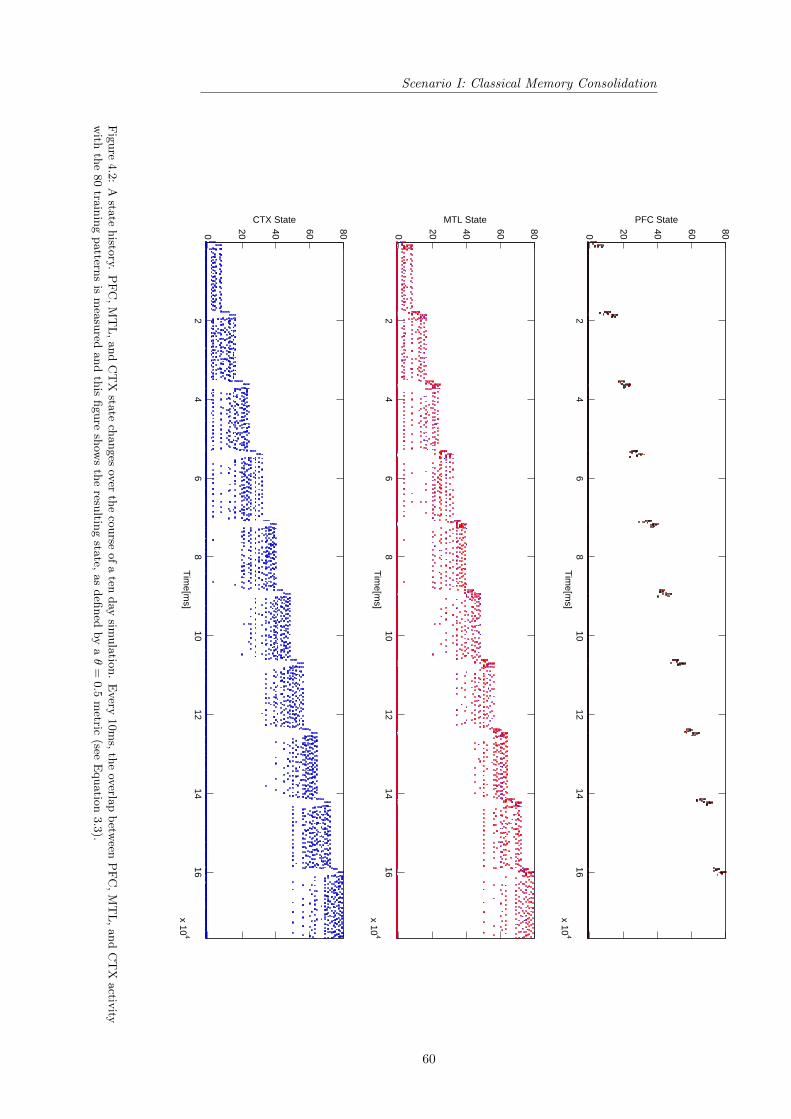
Scenario I: Classical Memory Consolidation
24
68
1012
1416
x 104
0 20 40 60 80
PFC StateT
ime[m
s]
24
68
1012
1416
x 104
0 20 40 60 80
MTL State
Tim
e[ms]
24
68
1012
1416
x 104
0 20 40 60 80
CTX State
Tim
e[ms]
Fig
ure
4.2
:A
state
histo
ry.P
FC
,M
TL
,and
CT
Xsta
tech
anges
over
the
course
of
aten
day
simula
tion.
Every
10m
s,th
eov
erlap
betw
eenP
FC
,M
TL
,and
CT
Xactiv
ityw
ithth
e80
train
ing
pattern
sis
mea
sured
and
this
figure
show
sth
eresu
lting
state,
as
defi
ned
by
aθ
=0.5
metric
(seeE
quatio
n3.3
).
60

Results
10 20 30 40 50 60 70 800
100200
PFC Total Pattern Activation Time
TP
AT
[ms]
10 20 30 40 50 60 70 800
10002000
MTL Total Pattern Activation Time
TP
AT
[ms]
10 20 30 40 50 60 70 800
5000CTX Total Pattern Activation Time
Pattern
TP
AT
[ms]
Figure 4.3: Total pattern activation time for all patterns in three memory stages.When compared to the simulation history in Figure 4.2, this is essentially a horizon-tal/temporal summation of the activity of each of the 80 states.
10 20 30 40 50 60 70 800
0.5
1PFC
Ret
rieva
ble
10 20 30 40 50 60 70 800
0.5
1MTL
Ret
rieva
ble
10 20 30 40 50 60 70 800
0.5
1CTX
Ret
rieva
ble
Pattern
Figure 4.4: Retrievable patterns after the ten day simulation run.
61

Scenario I: Classical Memory Consolidation
4.1.2 Generalized Scenario I Simulation
The system behavior is stochastic, especially due to the random degree of over-lap between patterns. To show the system properties more broadly, we alsoaverage the retrieval of 1000 simulation runs. Figure 4.5 shows the resultingretrieval rates ρPFC , ρMTL, and ρCTX depending on the pattern position. Theretrieval rate of patterns from the PFC peaks in the present, while the MTLand cortex achieve maximum consolidation somewhat later: The most retriev-able MTL pattern, ξ78, is a day old and the most consolidated cortical pattern,ξ64, with retrieval odds of above 50%, was introduced on day 8 and has thusbeen consolidated for three nights before retrieval testing.
0 10 20 30 40 50 60 70 800
0.5
1
Pro
babi
lity
Pattern
ρPFC
ρMTL
ρCTX
0 2 4 6 8 10 12 14 16 18 200
0.5
1
Pro
babi
lity
Percept
1 2 3 4 5 6 7 8 9 100
0.5
1
Pro
babi
lity
Completed day−night cycles
peak consolidationξ64 retrieval odds: 53%
Figure 4.5: Consolidation curves. 80 Patterns were introduced over the course of theten day simulation. Retrieval was averaged over 1000 simulations. Top panel: retrievalfrom all three memory stages depending on the pattern number (Pattern one is thefirst pattern, introduced in the first percept phase of day one. Pattern 80 is the lastpattern, introduced in the second percept phase of day ten.) Middle panel: Retrievalof patterns that were introduced in the same percept phase is averaged. Bottom panel:Retrieval of patterns introduced on the same day (eight per day) is averaged.
62

Results
4.2 Position-dependent Consolidation
Whatever we may think of the average consolidation performance seen in Fig-ure 4.5 (we will analyse the systemic behavior more completely in the Sec-tion 4.3.2), the remarkably periodic up-and-down of ρCTX in Figure 4.5 clearlydeserves some investigation. A period of eight patterns suggest, that there is astrong positional dependence of consolidation performance apart from the ex-pected consolidation delay and slow forgetting. By averaging the consolidationsuccess of all training patterns depending on their sequential position of intro-duction during their respective day-cycle, we obtain Figure 4.6.
1 2 3 4 5 6 7 80.1
0.15
0.2
0.25
0.3
0.35
0.4
0.45
0.5
Pattern Position
Avg
. Ret
rieva
l Pro
babi
lity
ρPFC
ρMTL
ρCTX
Figure 4.6: Cortical retrievalrates of patterns from differentpattern positions in the dailylearning queue. Retrieval for ear-lier patterns of each day is gen-erally worse. This can be at-tributed to partial overwriting bylater patterns before consolida-tion . The arrows mark unusuallyincreased retrieval rates from thecortex for pattern positions 4 and8.
Apart from the general trend toward better consolidation for later pattern posi-tions, noticeably every fourth pattern has an unusually improved performance.These are the last patterns of every percept. We are reminded of the positionaldependency of PFC replay performance in Figure 3.7. If the PFC is indeedthe cause for improved long-term consolidation success, then we should findthe same periodicity of four and eight in either the average number of patternreactivations (NPR) and/or total pattern reinstatement length (TPRL) duringreflections (NPR and TPRL were defined in Section 3.6).
10 20 30 40 50 60 70 80
0.8
1
1.2
1.4
1.6
1.8
PFC Pattern
NP
R
with resetwithout reset
10 20 30 40 50 60 70 8060
70
80
90
100
110
120
PFC Pattern
TP
RL
[ms]
with resetwithout reset
Figure 4.7: Periodicity of four in the number of pattern reactivations (NPR) and totalpattern reinstatement length (TPRL) during the reflection phases of complete tenday simulations. (NPR and TPRL were defined in Section 3.6.) With or withoutrandomization of PFC activity before replay. Averaged over 1000 runs each.
63
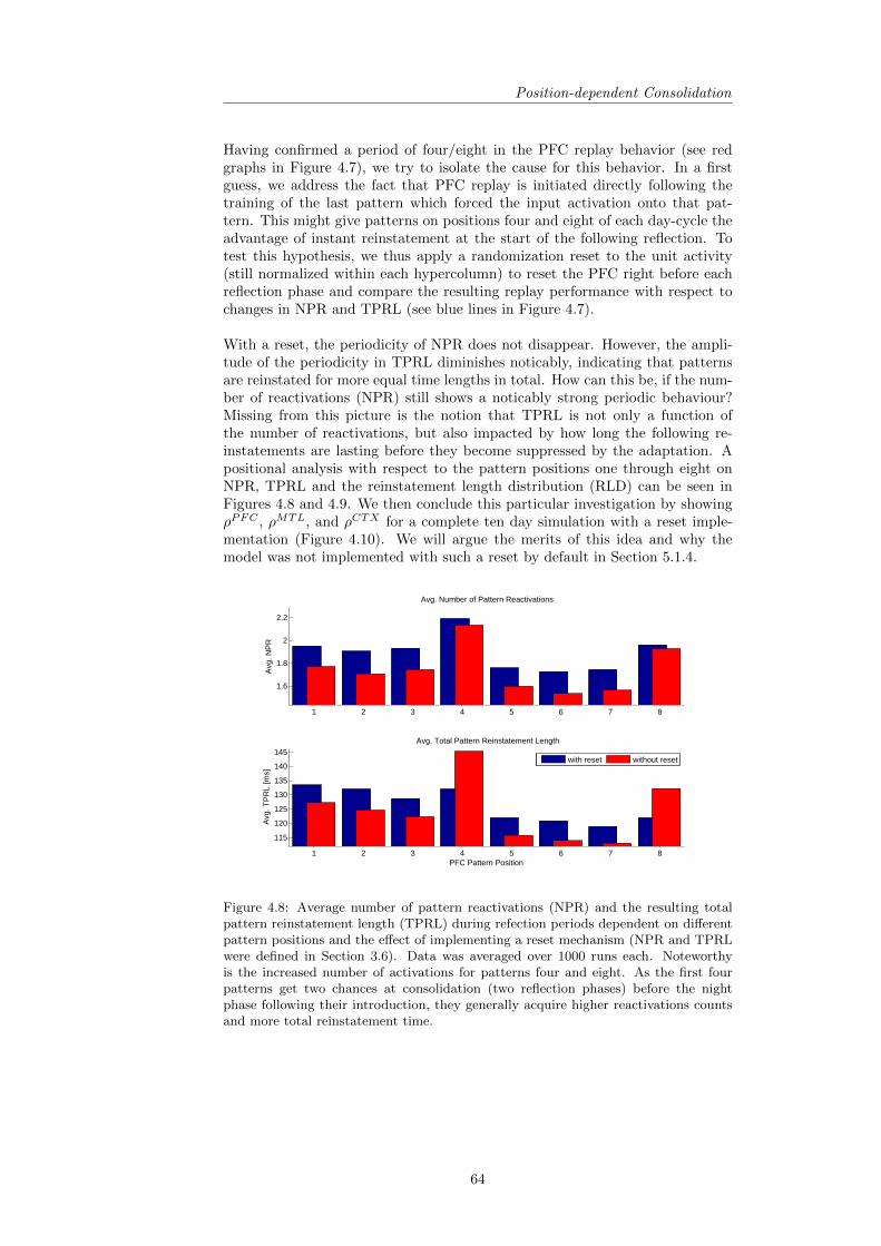
Position-dependent Consolidation
Having confirmed a period of four/eight in the PFC replay behavior (see redgraphs in Figure 4.7), we try to isolate the cause for this behavior. In a firstguess, we address the fact that PFC replay is initiated directly following thetraining of the last pattern which forced the input activation onto that pat-tern. This might give patterns on positions four and eight of each day-cycle theadvantage of instant reinstatement at the start of the following reflection. Totest this hypothesis, we thus apply a randomization reset to the unit activity(still normalized within each hypercolumn) to reset the PFC right before eachreflection phase and compare the resulting replay performance with respect tochanges in NPR and TPRL (see blue lines in Figure 4.7).
With a reset, the periodicity of NPR does not disappear. However, the ampli-tude of the periodicity in TPRL diminishes noticably, indicating that patternsare reinstated for more equal time lengths in total. How can this be, if the num-ber of reactivations (NPR) still shows a noticably strong periodic behaviour?Missing from this picture is the notion that TPRL is not only a function ofthe number of reactivations, but also impacted by how long the following re-instatements are lasting before they become suppressed by the adaptation. Apositional analysis with respect to the pattern positions one through eight onNPR, TPRL and the reinstatement length distribution (RLD) can be seen inFigures 4.8 and 4.9. We then conclude this particular investigation by showingρPFC , ρMTL, and ρCTX for a complete ten day simulation with a reset imple-mentation (Figure 4.10). We will argue the merits of this idea and why themodel was not implemented with such a reset by default in Section 5.1.4.
1 2 3 4 5 6 7 8
1.6
1.8
2
2.2
Avg
. NP
R
Avg. Number of Pattern Reactivations
1 2 3 4 5 6 7 8
115
120
125
130
135
140
145
Avg
. TP
RL
[ms]
Avg. Total Pattern Reinstatement Length
PFC Pattern Position
with reset without reset
Figure 4.8: Average number of pattern reactivations (NPR) and the resulting totalpattern reinstatement length (TPRL) during refection periods dependent on differentpattern positions and the effect of implementing a reset mechanism (NPR and TPRLwere defined in Section 3.6). Data was averaged over 1000 runs each. Noteworthyis the increased number of activations for patterns four and eight. As the first fourpatterns get two chances at consolidation (two reflection phases) before the nightphase following their introduction, they generally acquire higher reactivations countsand more total reinstatement time.
64

Results
0 20 40 60 80 100 120 140 1600
0.05
0.1
0.15
0.2P
roba
bilit
y
0 20 40 60 80 100 120 140 1600
0.05
0.1
0.15
0.2
Pro
babi
lity
Duration of pattern reinstatements
P1P2P3P4P5P6P7P8
With reset
Without reset
Figure 4.9: How long does a reinstatement last, before it becomes suppressed again?This figure shows the reinstatement length distribution (RLD) during reflection, de-pendent on different pattern positions (P1 through P8) and the effect of implementinga reset mechanism (RLD was defined in Section 3.6). Data was averaged over 1000runs each. Distributions on different positions are noticeably different, but similarevery four steps (ex. P1 and P5). Introducing a reset changes distributions P4 andP8 from a somewhat bimodal to a unimodal distribution.
0 10 20 30 40 50 60 70 800
0.5
1
Pro
babi
lity
Pattern
ρPFC
ρMTL
ρCTX
1 2 3 4 5 6 7 80.1
0.2
0.3
0.4
0.5
Pattern Position
Avg
. Ret
rieva
l Pro
babi
lity
Figure 4.10: Consolidation curves of a ten day simulation with a random reset ofactivity before each replay phase. This shows the odds of successful retrieval dependenton global pattern time/position (top) and the local pattern position within a day-cycle(bottom). Data was averaged over 1000 simulations. The arrows mark pattern positionfour and eight. The fourth pattern of every day still shows some unusually increasedperformance, despite the introduction of a reset. On position eight, the introduction ofa reset noticeably decreased retrieval. Variance in performance of patterns introducedon the same day is somewhat reduced, but overall, later patterns still exhibit higherconsolidation performance than earlier patterns of the same day.
65

Position-dependent Consolidation
The testing of positional dependence (serial position effects) in consolidation,motivated by observed oscillations in ρCTX , leads to several noteworthy obser-vations:
• Generally, pattern introduced in the first percept phase of each day (P1-P4) acquire a higher number of reactivations and longer total reinstate-ment (as can be seen in Figure 4.8) than patterns of the second daily per-cept (P5-P8). From the known positive correlation between reinstatementand cortical consolidation, we might expect that these patterns generallyconsolidate better, but the benefit of increased reinstatement is easilynegated by the partial overwriting that early patterns suffer by later pat-terns before the night phase starts. This weakens the relative strengthof their attractors right before this critical long-term consolidation phase.So in a paradoxical manner, later patterns generally consolidate better,despite lesser PFC reinstatement. This can be seen in the ascending slopein Figures 4.6 (without reset) and in the lower panel of Figure 4.10 (withreset).
• The patterns trained last in each perception phase are reactivated notice-ably more often than other patterns, as can be seen in the NPR of patternson position four (P4) and eight (P8) in Figures 4.7 and 4.8.
• Once activated, patterns trained last in each perception phase, are usu-ally instantiated for about the same time as other patterns (see RLD inFigure 4.9: The black distributions P4 and P8 in the lower part of thefigure are more spread, but have a similar mean compared to other distri-butions).
• As a result of the two above points, patterns trained last in a perceptionphase are consolidated for longer total time into the MTL and consequen-tially develop higher cortical retrieval rates over other patterns of the samepercept phase (See Figure 4.6. Additionally, note the significant positivecorrelation between TPRLPFC and ρCTX in Figure 4.18 and Table 4.1)
• Introducing a reset of activity before each replay phase levels the positionaldifferences in TPRL to a noticeable extent as can be seen in the flatteningof the curve in the lower panel of (Figure 4.8). But not due to a largechange in NPR, as we might have expected. In fact, the later, strongerpatterns retain a lot of their advantage here (see retained periodic peaksin the upper panel of Figure 4.8). Rather, most of the equalizing effectstems from a change in the distribution of pattern reinstatement lengths(see RLD in Figure 4.9: The black distributions P4, P8 show reducedchances for longer reinstatements (> 70ms) upon introduction of a reset).This can be explained by the following arguments:
– Strong/recent patterns such as patterns in positions P4, P8 convergegenerally faster, leading to shorter reinstatement periods. This canbe seen as an observable maximum in the probability distributionsnear 50 ms regardless of a reset (Figure 4.9).
– The reset now negates the previous guarantee of early reactivation.Since the first reactivation of any pattern is generally longer dueto lesser depression (due to pattern overlap and adaptation wind-up), this reduces the probability of long reactivations (> 70ms) forpositions P4, P8 noticeably. When P4 and P8 reactivate, the odds arehigher, that overlapping parts of their activity are already partiallydepressed. While this does not explain all the detail in Figure 4.9,it possibly hints toward the reason behind the unimodal/bimodalcharacter of the PRL distributions for P4, P8 with or without reset.
66

Results
• As a result of this dynamic, the introduction of a reset clearly diminishesthe periodicity of four patterns in the consolidation curve (see Figure 4.10).
• A periodic change in performance every eight patterns remains as an inher-ent property of the model and can not be eliminated by a reset mechanism(see Figure 4.10).
67
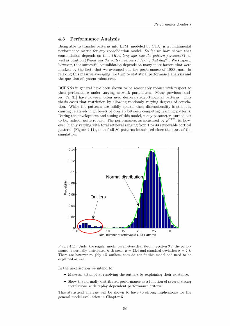
Performance Analysis
4.3 Performance Analysis
Being able to transfer patterns into LTM (modeled by CTX) is a fundamentalperformance metric for any consolidation model. So far we have shown thatconsolidation depends on time (How long ago was the pattern perceived? ) aswell as position (When was the pattern perceived during that day? ). We suspect,however, that successful consolidation depends on many more factors that weremasked by the fact, that we averaged out the performance of 1000 runs. Inrelaxing this massive averaging, we turn to statistical performance analysis andthe question of system robustness.
BCPNNs in general have been shown to be reasonably robust with respect totheir performance under varying network parameters. Many previous stud-ies [59, 31] have however often used decorrelated/orthogonal patterns. Thisthesis eases that restriction by allowing randomly varying degrees of correla-tion. While the patterns are mildly sparse, their dimensionality is still low,causing relatively high levels of overlap between competing training patterns.During the development and tuning of this model, many parameters turned outto be, indeed, quite robust. The performance, as measured by ρCTX , is, how-ever, highly varying with total retrieval ranging from 1 to 33 retrievable corticalpatterns (Figure 4.11), out of all 80 patterns introduced since the start of thesimulation.
0 5 10 15 20 25 300
0.02
0.04
0.06
0.08
0.1
0.12
0.14
Total number of retrievable CTX Patterns
Pro
babi
lity
Normal distribution
Outliers
Figure 4.11: Under the regular model parameters described in Section 3.2, the perfor-mance is normally distributed with mean µ = 23.4 and standard deviation σ = 2.8.There are however roughly 4% outliers, that do not fit this model and need to beexplained as well.
In the next section we intend to:
• Make an attempt at resolving the outliers by explaining their existence.
• Show the normally distributed performance as a function of several strongcorrelations with replay dependent performance criteria.
This statistical analysis will be shown to have to strong implications for thegeneral model evaluation in Chapter 5.
68

Results
4.3.1 Robustness of Performance
What exactly is going on inside the model when the performance unexpectedlydrops to the single digits? As an example of these rare cases, consider Fig-ure 4.12. Concluding a full ten day simulation, only a single pattern can beretrieved from the cortex. To clarify how this comes a bout we take a look atthe state history plot of said ten day simulation in Figure 4.13. After averageperformance for the first seven nights, it looks as though state 60 and 61 arecontinuously and simultaneously active throughout the last three nights. Weobviously know from the state definition in Equation 3.3, that only one pat-tern can be defined as active state at any given time. In fact, states 60 and61 alternate rapidly, switching back and fourth the state every iteration of thesimulation (dt=10ms) 33.
An overlap analysis also reveals, that the overlap with the corresponding train-ing patterns is weak, barely crossing the θ = 0.5 detection threshold. In apeculiar balance of associative attraction and adaptative repulsion the systemgets locked up in a tiny limit cycle of two noisy states. Patterns ξ60 and ξ61
converge so incompletely, that the neural and synaptic depression enacted inthe next time-step, will not push the activation away far enough such that thenetwork will not try to re-converge at the next step after being only weaklypushed out of a similarly weak attractor.
This situation agrees with the general conception, that weakly stored patternsare only visited for brief periods, but it breaks with the similar conception thatweakly stored patterns are visited fewer times. As a matter of fact, ξ60 and ξ61
are visited several thousand times during the last three nights. Interestinglyenough, this does not mean, that they become consolidated at all (see retrievalresults in Figure 4.12) because both MTL patterns are activated so weakly (nois-ily) that the projected cortical patterns 60 and 61 are similarly activated onlybarely above the detection threshold and will not be stored as correctly retriev-able patterns. Quite on the contrary, this weak activation causes the eventualdeletion of almost all prior memory in the cortex by essentially overloading thesystem with noise. From this perspective it is not all that astonishing thatonly a single training pattern, completely uncorrelated with ξ60 or ξ61, remainsretrievable.
10 20 30 40 50 60 70 800
0.5
1PFC
Ret
rieva
ble
10 20 30 40 50 60 70 800
0.5
1MTL
Ret
rieva
ble
10 20 30 40 50 60 70 800
0.5
1CTX
Ret
rieva
ble
Pattern
Figure 4.12: Retrievable patterns after a ten day simulation run
33States 60 and 61 are plotted as simultaneously active only due to insufficient temporalresolution on an A4-page. Zooming in on this part of the plot, we would be able to visualizethis ongoing alteration as well
69

Performance Analysis
24
68
1012
1416
x 104
0 20 40 60 80
PFC StateT
ime[m
s]
24
68
1012
1416
x 104
0 20 40 60 80
MTL State
Tim
e[ms]
24
68
1012
1416
x 104
0 20 40 60 80
CTX State
Tim
e[ms]
Fig
ure
4.1
3:
Exem
pla
rysta
tehisto
ryof
asim
ula
tion
classifi
edas
ap
erform
ance
outlier
due
toabnorm
al
beh
avio
rin
the
last
three
nig
ht
phases.
70

Results
Using a bit of statistical analysis, it is possible to show that this is indeed whathappens in virtually all cases of performance outliers. We start by taking a lookat the probability density functions behind NPR, RLD, and TPRL for the PFCin Figure 4.14. Overall, the lock-up problem does not seem to be an issue forthe PFC. The number of PFC pattern reactivations is completely distributedbetween zero and six, not what we would expect for cases of constant statealternation.
Next, we contrast these against the corresponding graphs for the MTL replaybehavior in Figures 4.15 and 4.16, where we can easily identify 0.1% of allpatterns that are reactivated thousands of times, while the large majority ofpatterns has much lower, normally distributed reactivation counts of up to onehundred times over the course of ten nights. We can see that outliers coincidewith extreme total pattern reinstatement lengths for the same small minorityof 0.1% of all patterns. Since the model becomes effectively locked for all futurelearning in the event of such a pattern, and past learning gets largely deletedas well, this small minority of patterns can cause a noticeable amount of per-formance outliers.
0 1 2 3 4 5 60
0.2
0.4
0.6
NPRPFC
Pro
babi
lity
50 100 150 200 250 300 350 4000
0.05
0.1
0.15
RLDPFC
Pro
babi
lity
0 200 400 600 800 10000
0.1
0.2
0.3
TPRLPFC
Pro
babi
lity
Figure 4.14: Probability density functions of PFC replay performance, averaged overall reflection periods. (NPR, RLD and TPRL were defined in Section 3.6.) Mostpatterns are reactivated one or two times (see NPR) for a reinstatement of 50-100 ms(see RLD) and thus acquire between 100 and 200 ms of total pattern reinstatement(see TPRL).
71
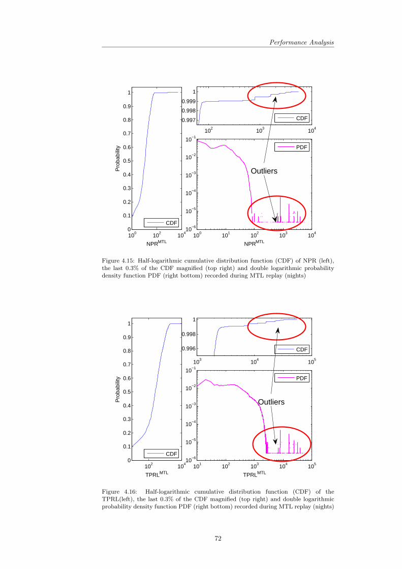
Performance Analysis
100 102 1040
0.1
0.2
0.3
0.4
0.5
0.6
0.7
0.8
0.9
1
NPRMTL
Pro
babi
lity
CDF
102 103 104
0.997
0.998
0.999
1
CDF
100 101 102 103 10410−6
10−5
10−4
10−3
10−2
10−1
NPRMTL
Outliers
Figure 4.15: Half-logarithmic cumulative distribution function (CDF) of NPR (left),the last 0.3% of the CDF magnified (top right) and double logarithmic probabilitydensity function PDF (right bottom) recorded during MTL replay (nights)
102 1040
0.1
0.2
0.3
0.4
0.5
0.6
0.7
0.8
0.9
1
TPRLMTL
Pro
babi
lity
CDF
103 104 105
0.996
0.998
1
CDF
101 102 103 104 10510−6
10−5
10−4
10−3
10−2
10−1
TPRLMTL
Outliers
Figure 4.16: Half-logarithmic cumulative distribution function (CDF) of theTPRL(left), the last 0.3% of the CDF magnified (top right) and double logarithmicprobability density function PDF (right bottom) recorded during MTL replay (nights)
72
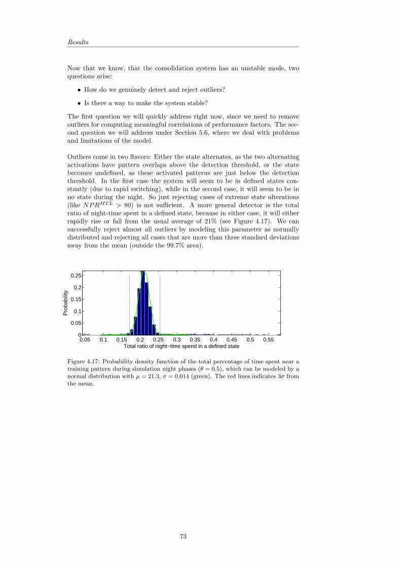
Results
Now that we know, that the consolidation system has an unstable mode, twoquestions arise:
• How do we genuinely detect and reject outliers?
• Is there a way to make the system stable?
The first question we will quickly address right now, since we need to removeoutliers for computing meaningful correlations of performance factors. The sec-ond question we will address under Section 5.6, where we deal with problemsand limitations of the model.
Outliers come in two flavors: Either the state alternates, as the two alternatingactivations have pattern overlaps above the detection threshold, or the statebecomes undefined, as these activated patterns are just below the detectionthreshold. In the first case the system will seem to be in defined states con-stantly (due to rapid switching), while in the second case, it will seem to be inno state during the night. So just rejecting cases of extreme state alterations(like NPRMTL > 80) is not sufficient. A more general detector is the totalratio of night-time spent in a defined state, because in either case, it will eitherrapidly rise or fall from the usual average of 21% (see Figure 4.17). We cansuccessfully reject almost all outliers by modeling this parameter as normallydistributed and rejecting all cases that are more than three standard deviationsaway from the mean (outside the 99.7% area).
0.05 0.1 0.15 0.2 0.25 0.3 0.35 0.4 0.45 0.5 0.550
0.05
0.1
0.15
0.2
0.25
Total ratio of night−time spend in a defined state
Pro
babi
lity
Figure 4.17: Probability density function of the total percentage of time spent near atraining pattern during simulation night phases (θ = 0.5), which can be modeled by anormal distribution with µ = 21.3, σ = 0.014 (green). The red lines indicates 3σ fromthe mean.
73
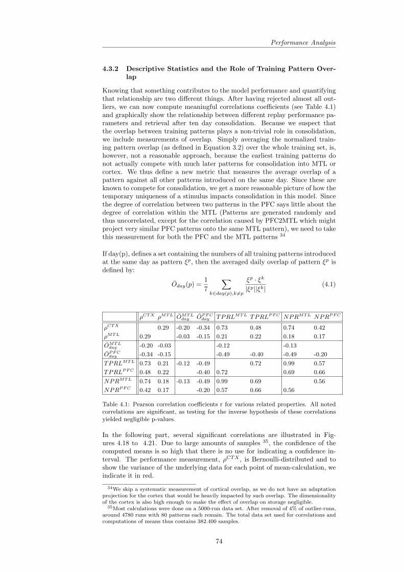
Performance Analysis
4.3.2 Descriptive Statistics and the Role of Training Pattern Over-lap
Knowing that something contributes to the model performance and quantifyingthat relationship are two different things. After having rejected almost all out-liers, we can now compute meaningful correlations coefficients (see Table 4.1)and graphically show the relationship between different replay performance pa-rameters and retrieval after ten day consolidation. Because we suspect thatthe overlap between training patterns plays a non-trivial role in consolidation,we include measurements of overlap. Simply averaging the normalized train-ing pattern overlap (as defined in Equation 3.2) over the whole training set, is,however, not a reasonable approach, because the earliest training patterns donot actually compete with much later patterns for consolidation into MTL orcortex. We thus define a new metric that measures the average overlap of apattern against all other patterns introduced on the same day. Since these areknown to compete for consolidation, we get a more reasonable picture of how thetemporary uniqueness of a stimulus impacts consolidation in this model. Sincethe degree of correlation between two patterns in the PFC says little about thedegree of correlation within the MTL (Patterns are generated randomly andthus uncorrelated, except for the correlation caused by PFC2MTL which mightproject very similar PFC patterns onto the same MTL pattern), we need to takethis measurement for both the PFC and the MTL patterns 34
If day(p), defines a set containing the numbers of all training patterns introducedat the same day as pattern ξp, then the averaged daily overlap of pattern ξp isdefined by:
Oday(p) =1
7
∑k∈day(p),k 6=p
ξp · ξk
|ξp||ξk|(4.1)
ρCTX ρMTL OMTLday OPFC
day TPRLMTL TPRLPFC NPRMTL NPRPFC
ρCTX 0.29 -0.20 -0.34 0.73 0.48 0.74 0.42
ρMTL 0.29 -0.03 -0.15 0.21 0.22 0.18 0.17
OMTLday -0.20 -0.03 -0.12 -0.13
OPFCday -0.34 -0.15 -0.49 -0.40 -0.49 -0.20
TPRLMTL 0.73 0.21 -0.12 -0.49 0.72 0.99 0.57
TPRLPFC 0.48 0.22 -0.40 0.72 0.69 0.66
NPRMTL 0.74 0.18 -0.13 -0.49 0.99 0.69 0.56
NPRPFC 0.42 0.17 -0.20 0.57 0.66 0.56
Table 4.1: Pearson correlation coefficients r for various related properties. All notedcorrelations are significant, as testing for the inverse hypothesis of these correlationsyielded negligible p-values.
In the following part, several significant correlations are illustrated in Fig-ures 4.18 to 4.21. Due to large amounts of samples 35, the confidence of thecomputed means is so high that there is no use for indicating a confidence in-terval. The performance measurement, ρCTX , is Bernoulli-distributed and toshow the variance of the underlying data for each point of mean-calculation, weindicate it in red.
34We skip a systematic measurement of cortical overlap, as we do not have an adaptationprojection for the cortex that would be heavily impacted by such overlap. The dimensionalityof the cortex is also high enough to make the effect of overlap on storage negligible.
35Most calculations were done on a 5000-run data set. After removal of 4% of outlier-runs,around 4780 runs with 80 patterns each remain. The total data set used for correlations andcomputations of means thus contains 382.400 samples.
74

Results
4.3.3 Evaluating the found Correlations
The correlation analysis (see Table 4.1) largely confirmed what we knew aboutthe behavior of a BCPNN upon introduction of an adaptation based in synap-tic and neural depression. The number of reactivations and the total time ofpattern reinstatement are highly correlated (r(NPRMTL, TPRLMTL) = 0.99),strongly encoded patterns are reactivated more often during adaptation drivenreplay and while the MTL activity is a better predictor of the overall long-termconsolidation success (r(ρCTX , TPRLMTL) = 0.73), than the preceding PFCactivity (r(ρCTX , TPRLPFC) = 0.48), it is the degree of correlation of a train-ing pattern in the PFC, that matters more than the same measure taken inthe MTL(r(ρCTX , OPFCday ) = −0.34 and r(ρCTX , OMTL
day ) = −0.20). As AndersSandberg correctly pointed out in his dissertation [59, p.79], the effect of corre-lation diminishes with the size of the network.
4.3.4 Revisiting the Predictions
Prediction I: We expect MTL consolidation to be near 100% afteronly one day.
This is easily proven correct by the MTL consolidation curve in red in Figure 4.5,showing more than 90% of the patterns from the previous day to be retrievablefrom the MTL.
Prediction II: We expect to be able to retrieve stored MTL pat-terns for about four days once they have been consolidated.
As the MTL forgets very gradually (ρMTL is almost linear between two and fourday old patterns), this is a bit difficult to argue. However, after about four daysthe probability of successful MTL retrieval has dropped to 19% and virtuallyno MTL pattern older than 6 days can be retrieved.
Prediction IIIa: Complete long-term consolidation takes aboutthree days/nights.
Actually consolidation occurs slightly faster than expected. The cortex consol-idation curve shows maximum consolidation after only two nights. The mostretrievable pattern, ξ64, however, has indeed been consolidated for three nights.
Prediction IIIb: Successful long-term consolidation requires about1333 ms of total reinstatement.
The analysis in Section 4.3.2 shows a strong correlation between TPRLMTL andρCTX with Pearson coefficient k=73%. Figure 4.18 confirms a 97% retrieval rateafter 1350 ms of reinstatement. Only 5% of patterns are reinstated longer thanthat (see cumulative distribution function in Figure 4.16). Shorter reinstatementmostly increases the variance in the retrieval rate. Only under 1000 ms totalreinstatement length does the averaged retrieval rate fall below 90%.
Prediction IV: We expect roughly 33% of all patterns to be con-solidated into long-term memory.
With ρCTX ranging from 10% to 53% and a mean of 28%, the overall perfor-mance is slightly lower than predicted.
Prediction V: We expect the cortex to retain retrieval of someconsolidated patterns about 2 weeks.
75
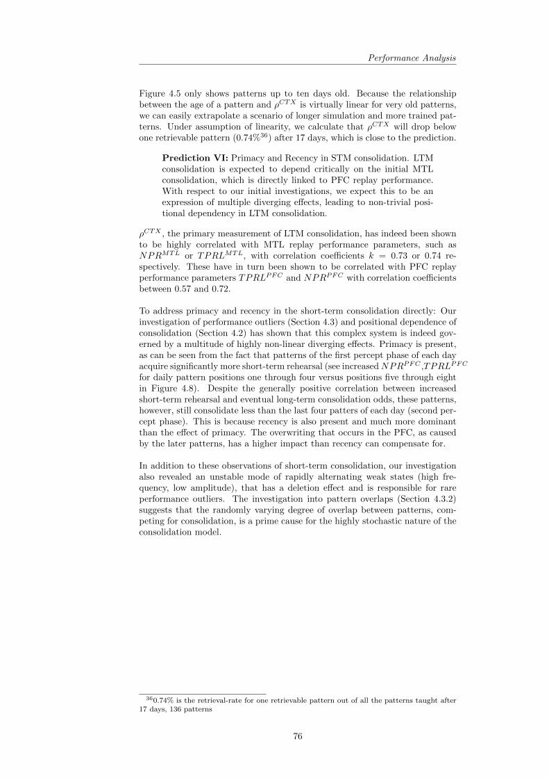
Performance Analysis
Figure 4.5 only shows patterns up to ten days old. Because the relationshipbetween the age of a pattern and ρCTX is virtually linear for very old patterns,we can easily extrapolate a scenario of longer simulation and more trained pat-terns. Under assumption of linearity, we calculate that ρCTX will drop belowone retrievable pattern (0.74%36) after 17 days, which is close to the prediction.
Prediction VI: Primacy and Recency in STM consolidation. LTMconsolidation is expected to depend critically on the initial MTLconsolidation, which is directly linked to PFC replay performance.With respect to our initial investigations, we expect this to be anexpression of multiple diverging effects, leading to non-trivial posi-tional dependency in LTM consolidation.
ρCTX , the primary measurement of LTM consolidation, has indeed been shownto be highly correlated with MTL replay performance parameters, such asNPRMTL or TPRLMTL, with correlation coefficients k = 0.73 or 0.74 re-spectively. These have in turn been shown to be correlated with PFC replayperformance parameters TPRLPFC and NPRPFC with correlation coefficientsbetween 0.57 and 0.72.
To address primacy and recency in the short-term consolidation directly: Ourinvestigation of performance outliers (Section 4.3) and positional dependence ofconsolidation (Section 4.2) has shown that this complex system is indeed gov-erned by a multitude of highly non-linear diverging effects. Primacy is present,as can be seen from the fact that patterns of the first percept phase of each dayacquire significantly more short-term rehearsal (see increasedNPRPFC ,TPRLPFC
for daily pattern positions one through four versus positions five through eightin Figure 4.8). Despite the generally positive correlation between increasedshort-term rehearsal and eventual long-term consolidation odds, these patterns,however, still consolidate less than the last four patters of each day (second per-cept phase). This is because recency is also present and much more dominantthan the effect of primacy. The overwriting that occurs in the PFC, as causedby the later patterns, has a higher impact than recency can compensate for.
In addition to these observations of short-term consolidation, our investigationalso revealed an unstable mode of rapidly alternating weak states (high fre-quency, low amplitude), that has a deletion effect and is responsible for rareperformance outliers. The investigation into pattern overlaps (Section 4.3.2)suggests that the randomly varying degree of overlap between patterns, com-peting for consolidation, is a prime cause for the highly stochastic nature of theconsolidation model.
360.74% is the retrieval-rate for one retrievable pattern out of all the patterns taught after17 days, 136 patterns
76

Results
0 2 4 60
0.2
0.4
0.6
0.8
1
NPRPFC0 20 40 60 80
0
0.2
0.4
0.6
0.8
1
NPRMTL
ρCTX Var(ρCTX)
0 50 1000
0.2
0.4
0.6
0.8
1
TPRLPFC0 1000 2000 3000 4000
0
0.2
0.4
0.6
0.8
1
TPRLMTL
Figure 4.18: Important relationships between replay performance and successful con-solidation as measured by ρCTX . NPR and TPRL denote the number of patternreactivations and the total pattern reinstatement length, both defined in Section 3.6.
0 20 40 60 800
500
1000
1500
2000
2500
NPRMTL
TP
RLM
TL
0 1 2 3 4 50
500
1000
1500
2000
2500
NPRPFC
TP
RLM
TL
0 20 40 60 800
100
200
300
400
500
600
NPRMTL
TP
RLP
FC
0 1 2 3 4 50
100
200
300
400
500
600
NPRPFC
TP
RLP
FC
r=0.69
r=0.99 r=0.57
r=0.66
Figure 4.19: Scatter plots of relationships between different replay phases. The 1000scatter points correspond to patterns, that were sampled randomly from the data.During reflections, a measure of the number of reactivations and total reactivationlength for each pattern was recorded (NPRPFC and TPRLPFC). During the nightphase, these quantities were measured in the MTL (NPRMTL and TPRLMTL). Thevalue r indicates the corresponding Pearson correlation coefficient from Table 4.1.
77

Performance Analysis
0 0.1 0.2 0.30
0.05
0.1
0.15
0.2
DailyAvg.OverlapPFC
Pro
babi
lity
0 0.1 0.2 0.30
0.2
0.4
0.6
0.8
1
DailyAvg.OverlapPFC
ρCTX
Var(ρCTX)
0 0.05 0.1 0.15 0.2 0.250
0.05
0.1
DailyAvg.OverlapMTL
Pro
babi
lity
0 0.05 0.1 0.15 0.2 0.250
0.2
0.4
0.6
0.8
1
DailyAvg.OverlapMTL
ρCTX
Var(ρCTX)
Figure 4.20: The distribution of training pattern overlap (left) and its impact on longterm consolidation (right) for the PFC (top) and the MTL (bottom). The variance ofthe underlying data is shown in red.
0 0.05 0.1 0.15 0.2 0.25 0.30
500
1000
1500
2000
DailyAvg.OverlapPFC
TP
RLM
TL
0 0.05 0.1 0.15 0.2 0.25 0.30
200
400
600
DailyAvg.OverlapPFC
TP
RLP
FC
Figure 4.21: The impact of training pattern overlap in the PFC on the total patternreinstatement length resulting in the PFC and MTL. The error bars indicate twostandard deviations, showing roughly the 95% interval of the underlying data
78

Results
4.4 Scenario II: Learning Time Constant Modulations
In this section, we implement several possible plasticity modulations by manip-ulating the learning time constants. This is done through the introduction ofa relevance signal κ(t). Depending on where we apply the modulation (PFC,MTL, or CTX), this can be interpreted as an attempt to build a mechanismakin to an operational attentional gate, simulate dopaminergic plasticity modu-lation (see Section 2.1.3), or a model of other contextual and relational relevancemodulations. κ(t) thus surmises a multitude of memory modulations observedin real life, ranging from stimulus intensity and meaning-based, contextual orrelational factors, including emotional significance, to conscious attention, ornovelty of a stimulus.
The following approach was originally proposed by Lansner and Ekeberg [33] andexperimentally investigated by Sandberg [59] in 2003. It is a slight modificationof the original BCPNN learning rule, that allows for a selective increase ordecrease of the learning rate.
Λii′(t) = Λii′(t− 1) +κ(t)
τL[πii′(t)− Λii′(t− 1)] (4.2)
Λii′jj′(t) = Λii′jj′(t− 1) +κ(t)
τL[πii′(t)πjj′(t)− Λii′jj′(t− 1)] (4.3)
Generally, we keep κ(t) = 1, except for specified training patterns within thetraining set –here called isolates– for whom we set κ(t) = κi. To average outthe overall time/position-dependence of consolidation as well as positional de-pendence within the learning stack, we select patterns at varying positions tobecome isolates for testing, while also varying κi over a range of suitable values.This means, that we test scenarios between no learning and highly increasedlearning rates for the isolate(s) among an otherwise normally learning popula-tion of BCPNN units. A systematic introduction and performance model forthis kind of modulation during direct training (no replay mechanics involved)can be found in [59, Ch.4]. Here, we apply it during replay-driven memoryconsolidation.
We start with implementing a PFC modulation (Figure 4.22) and show its effecton the cortical retrieval rate of the isolate. This modulation allows us to modifythe PFC learning rate for the isolate and can be interpreted as a modulationof stimulation intensity or an attentional gate. For κPFC = 0, the isolate isnot perceived at all. Next, we implement a MTL modulation which allows usto modify MTL encoding of the isolate during reflection by changing κMTL
(Figure 4.23). Figure 4.24 then shows a similar modulation for cortical learningduring the night, and finally, Figure 4.25 shows a general modulation acrossall three stages. For better illustration of what is happening not just withthe isolate, but also its neighboring patterns, we also show an example of thisgeneral modulation. In Figure 4.26, the isolate ξ60, has been modulated withκ = 2 and the resulting retrieval rates for all patterns is shown.
79

Scenario II: Learning Time Constant Modulations
0 0.5 1 1.5 20
0.2
0.4
0.6
0.8
1
ρCT
X
PFC Modulation kPFC
ρCTX Var(ρCTX)
Figure 4.22: Introducing a PFC modulation κPFC . ρCTX indicates the averaged cortexretrieval rate of the isolate after a ten day simulation. The variance of the underlyingdata is shown in red.
0 1 2 3 40
0.2
0.4
0.6
0.8
1
ρCT
X
MTL Modulation kMTL
ρCTX Var(ρCTX)
Figure 4.23: Introducing an attentional gate factor κMTL. ρCTX indicates the averagedcortex retrieval rate of the isolate after a ten day simulation. The variance of theunderlying data is shown in red.
0 5 10 150
0.2
0.4
0.6
0.8
1
ρCT
X
CTX Modulation kCTX
ρCTX
Var(ρCTX)
Figure 4.24: Introducing an relevance modulation κCTX . ρCTX indicates the averagedcortex retrieval rate of the isolate after a ten day simulation. The variance of theunderlying data is shown in red.
80
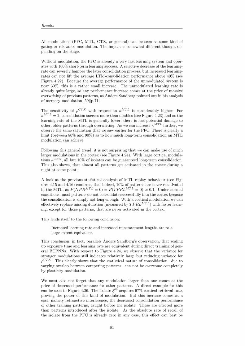
Results
All modulations (PFC, MTL, CTX, or general) can be seen as some kind ofgating or relevance modulation. The impact is somewhat different though, de-pending on the stage.
Without modulation, the PFC is already a very fast learning system and oper-ates with 100% short-term learning success. A selective decrease of the learning-rate can severely hamper the later consolidation process, but increased learning-rates can not lift the average LTM-consolidation performance above 40% (seeFigure 4.22). Because the average performance of the unmodulated system isnear 30%, this is a rather small increase. The unmodulated learning rate isalready quite large, so any performance increase comes at the price of massiveoverwriting of previous patterns, as Anders Sandberg pointed out in his analysisof memory modulation [59][p.71].
The sensitivity of ρCTX with respect to κMTL is considerably higher: ForκMTL = 2, consolidation success more than doubles (see Figure 4.23) and as thelearning rate of the MTL is generally lower, there is less potential damage toother, older patterns through overwriting. As we can increase κMTL further, weobserve the same saturation that we saw earlier for the PFC. There is clearly alimit (between 80% and 90%) as to how much long-term consolidation an MTLmodulation can achieve.
Following this general trend, it is not surprising that we can make use of muchlarger modulations in the cortex (see Figure 4.24). With large cortical modula-tions κCTX , all but 10% of isolates can be guaranteed long-term consolidation.This also shows, that almost all patterns get activated in the cortex during anight at some point:
A look at the previous statistical analysis of MTL replay behaviour (see Fig-ures 4.15 and 4.16) confirms, that indeed, 10% of patterns are never reactivatedin the MTL, as P (NPRMTL = 0) = P (TPRLMTL = 0) ' 0.1. Under normalconditions, most patterns do not consolidate successfully into the cortex becausethe consolidation is simply not long enough. With a cortical modulation we caneffectively replace missing duration (measured by TPRLMTL) with faster learn-ing, except for those patterns, that are never activated in the cortex.
This lends itself to the following conclusion:
Increased learning rate and increased reinstatement lengths are to alarge extent equivalent.
This conclusion, in fact, parallels Anders Sandberg’s observation, that scalingup exposure time and learning rate are equivalent during direct training of gen-eral BCPNNs. With respect to Figure 4.24, we observe that the variance forstronger modulations still indicates relatively large but reducing variance forρCTX . This clearly shows that the statistical nature of consolidation –due tovarying overlap between competing patterns– can not be overcome completelyby plasticity modulation.
We must also not forget that any modulation larger than one comes at theprice of decreased performance for other patterns. A direct example for thiscan be seen in Figure 4.26. The isolate ξ60 acquires 97% cortical retrieval rate,proving the power of this kind of modulation. But this increase comes at acost, namely retroactive interference, the decreased consolidation performanceof other training patterns, taught before the isolate. These are effected morethan patterns introduced after the isolate. As the absolute rate of recall ofthe isolate from the PFC is already zero in any case, this effect can best be
81
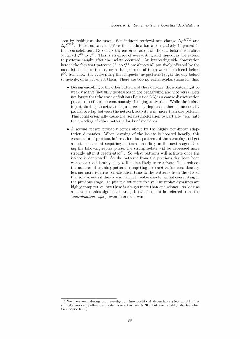
Scenario II: Learning Time Constant Modulations
seen by looking at the modulation induced retrieval rate change ∆ρMTL and∆ρCTX . Patterns taught before the modulation are negatively impacted intheir consolidation. Especially the patterns taught on the day before the isolateoccurred ξ49 to ξ56. This is an effect of overwriting and thus does not extendto patterns taught after the isolate occurred. An interesting side observationhere is the fact that patterns ξ57 to ξ64 are almost all positively affected by themodulation of the isolate, even though some of them were introduced beforeξ60. Somehow, the overwriting that impacts the patterns taught the day beforeso heavily, does not effect them. There are two potential explanations for this:
• During encoding of the other patterns of the same day, the isolate might beweakly active (not fully depressed) in the background and vice versa. Letsnot forget that the state definition (Equation 3.3) is a coarse discretizationput on top of a more continuously changing activation. While the isolateis just starting to activate or just recently depressed, there is necessarilypartial overlap between the network activity with more than one pattern.This could essentially cause the isolates modulation to partially ’leak’ intothe encoding of other patterns for brief moments.
• A second reason probably comes about by the highly non-linear adap-tation dynamics. When learning of the isolate is boosted heavily, thiserases a lot of previous information, but patterns of the same day still geta better chance at acquiring sufficient encoding on the next stage: Dur-ing the following replay phase, the strong isolate will be depressed morestrongly after it reactivated37. So what patterns will activate once theisolate is depressed? As the patterns from the previous day have beenweakened considerably, they will be less likely to reactivate. This reducesthe number of training patterns competing for reactivation considerably,leaving more relative consolidation time to the patterns from the day ofthe isolate, even if they are somewhat weaker due to partial overwriting inthe previous stage. To put it a bit more freely: The replay dynamics arehighly competitive, but there is always more than one winner. As long asa pattern retains significant strength (which might be referred to as the’consolidation edge’), even losers will win.
37We have seen during our investigation into positional dependence (Section 4.2, thatstrongly encoded patterns activate more often (see NPR), but even slightly shorter whenthey do(see RLD)
82

Results
0 1 2 3 40
0.2
0.4
0.6
0.8
1
ρCT
X
General Modulation kPFC=kMTLkCTX
ρCTX
Var(ρCTX)
Figure 4.25: Introducing an general modulation across all three memory stages. ρCTX
indicates the averaged cortex retrieval rate of the isolate after a ten day simulation.The variance of the underlying data is shown in red.
0 10 20 30 40 50 60 70 800
0.2
0.4
0.6
0.8
1
Pro
babi
lity
Pattern
ρPFCmodulated
ρMTLmodulated
ρCTXmodulated
ρPFCunmodulated
ρMTLunmodulated
ρCTXunmodulated
10 20 30 40 50 60 70 80
−0.1
0
0.1
0.2
0.3
0.4
0.5
Rel
ativ
e pr
obab
ility
cha
nge
Pattern
∆ρCTX
∆ρMTL
Figure 4.26: An example of what happens to retrieval in the general modulation casefor i=60 and κi = 2. The upper figure shows retrieval rates of the modulated system,as well as the retrieval rates of an unmodulated system for comparison. The lowerpart shows the relative change in retrieval rates for MTL and cortex.
83
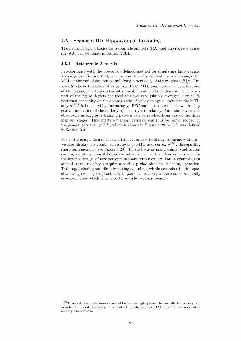
Scenario III: Hippocampal Lesioning
4.5 Scenario III: Hippocampal Lesioning
The neurobiological basics for retrograde amnesia (RA) and anterograde amne-sia (AA) can be found in Section 2.3.4.
4.5.1 Retrograde Amnesia
In accordance with the previously defined method for simulating hippocampallesioning (see Section 3.7), we now run ten day simulations and damage theMTL at the end of day ten by nullifying a portion χ of the weights wMTL
ii′jj′ . Fig-
ure 4.27 shows the retrieval rates from PFC, MTL ,and cortex 38, as a functionof the training patterns retrievable on different levels of damage. The lowerpart of the figure depicts the total retrieval rate (simply averaged over all 80patterns) depending on the damage ratio. As the damage is limited to the MTL,only ρMTL is impacted by increasing χ. PFC and cortex are still shown, as theygive an indication of the underlying memory redundancy. Amnesia may not beobservable as long as a training pattern can be recalled from any of the threememory stages. This effective memory retrieval can thus be better judged bythe general retrieval, ρPMC , which is shown in Figure 4.28 (ρPMC was definedin Section 3.3).
For better comparison of the simulation results with biological memory studies,we also display the combined retrieval of MTL and cortex ρMC , disregardingshort-term memory (see Figure 4.29). This is because many animal studies con-cerning long-term consolidation are set up in a way that does not account forthe fleeting storage of new percepts in short-term memory. For an example, testanimals (rats, monkeys) require a resting period after the lesioning operation.Training, lesioning and directly testing an animal within seconds (the timespanof working memory) is practically impossible. Rather, test are done on a dailyor weekly basis which thus need to exclude working memory.
38These retrieval rates were measured before the night phase, that usually follows day ten,in order to seperate the measurement of retrograde amnesia (RA) from the measurement ofanterograde amnesia.
84

Results
354045505560657075800
0.1
0.2
0.3
0.4
0.5
0.6
0.7
0.8
0.9
1
Pattern
Ret
rieva
l Rat
e
ρPFC
ρMTLχ=0%
ρMTLχ=20%
ρMTLχ=40%
ρMTLχ=60%
ρMTLχ=80%
ρCTX
0 0.1 0.2 0.3 0.4 0.5 0.6 0.7 0.8 0.9 10
0.1
0.2
0.3
0.4
MTL damage ratio χ
Avg
. Ret
rieva
l Rat
e
ρPFC
ρMTL
ρCTX
Figure 4.27: Retrieval rates after simulated hippocampal lesioning χ. While previouslystored PFC and cortical patterns are not affected, the MTL steadily looses more andmore memory of the stored patterns when the MTL is increasingly lesioned.
354045505560657075800
0.1
0.2
0.3
0.4
0.5
0.6
0.7
0.8
0.9
1
Pattern
Ret
rieva
l Rat
e
ρPMC
χ=0%
ρPMCχ=20%
ρPMCχ=40%
ρPMCχ=60%
ρPMCχ=80%
ρPFC
ρCTX
56789100
0.2
0.4
0.6
0.8
1
Day
Ret
rieva
l Rat
e
Figure 4.28: Overall retrieval rate ,ρPMC , after simulated hippocampal lesioning χ.Only patterns 32 to 80 (days five to ten) are shown, as the damage ratio has no effecton older patterns. In the lower part of the figure, retrieval rates of the eight patternsof each day were averaged to disregard the daily positional dependence.
85

Scenario III: Hippocampal Lesioning
354045505560657075800
0.1
0.2
0.3
0.4
0.5
0.6
0.7
0.8
0.9
1
Pattern
Ret
rieva
l Rat
e
ρMC
χ=0%
ρMCχ=20%
ρMCχ=40%
ρMCχ=60%
ρMCχ=80%
ρCTX
56789100
0.5
1
Day
Avg
. Ret
rieva
l Rat
e
Figure 4.29: Overall retrieval rate ρMC after simulated hippocampal lesioning χ. Onlypatterns 32 to 80 (days five to ten) are shown, as the damage ratio has no effect onolder patterns. In the lower part of the figure, retrieval rates of the eight patterns ofeach day were averaged to disregard the daily positional dependence.
Testing shows significant retrograde amnesia (RA) as a result of simulated hip-pocampal lesioning. Looking at the retrieval rates of the undamaged system forthe PFC (black), MTL (red) and CTX (blue) in Figure 4.27, we can see, thatthe MTL normally bridges the gap between the most recent patterns, stored inthe PFC, and remote, cortically consolidated patterns. Hippocampal lesioningreduces retrieval for all MTL patterns, with higher sensitivity for very recentand very remote patterns (ρMTL develops a maximum near ξ77 for increasingdamage). This is not surprising and squares reasonably with Ribot’s Law (seeSection 2.3.4), as not fully learned or almost forgotten training patterns are morevulnerable to disruptions in their support that may occur due to the growingnumber of connections cut by the damage.
The typical symptoms of temporally graded RA in a multi-stage memory systemis the curious gap in retrieval rates between intact STM and LTM memories,both of which are left intact after hippocampal lesioning (see Section 2.3.4).For the case of patient HM, we stated that his retrograde amnesia was tempo-rally graded after hippocampal lesioning: He had intact STM/WM and LTM,but lost all memory of the recent past right after his operation. This exactphenomenon can be observed in this connectionist model as well. Figure 4.28shows the general retrieval ρPMC . Very recent memories are supported by thePFC, very remote memories by the cortex. The MTL usually fills the gap. Soupon introduction of hippocampal lesioning, we loose memories mostly in thismid-term memory area. The retrieval of training patterns, ξ64 to ξ72, whichare not yet fully consolidated into the cortex, is most heavily impacted by sim-ulated hippocampal damage. The amnesia is temporally graded, because theeffect of simulated hippocampal damage gradually becomes less pronounced forolder patterns. For patterns more than five days old, simulated hippocampallesioning has only a negligible effect on overall retrieval.
86

Results
4.5.2 Anterograde Amnesia
For testing anterograde amnesia (AA) in this model, we now attempt memoryconsolidation in a system that has undergone simulated hippocampal lesioning.As usual, we test training pattern retrieval after the tenth day. The averagedretrieval rates of 1000 runs after different levels of hippocampal damage can beseen in Figure 4.30. The overall retrieval ρPMC is determined and, as expected,the system memory consolidation system capability is impaired and the overallretrieval after a ten day simulation can be seen in Figure 4.31.
4.5.3 Comparing RA and AA
The most obvious difference between both forms of amnesia is the fact that RAis restricted to the MTL and thus temporally graded, effecting only patternsless than five days old. AA is however not temporally graded. It affects allfuture patterns equally, right from the moment of lesioning. The damage to theMTL network leaves cortical memories intact, but it permanently damages thememory consolidation capability of the system. At χ = 60%, the system be-comes completely incapable of forming any new long-term memory, despite thefact that the cortex itself has not sustained any damage. At around χ = 70%damage, the acquisition of patterns into the MTL becomes negligible as well.The system is left with only its modest STM capabilites, which stem from theintact and unaffected PFC.
87

Scenario III: Hippocampal Lesioning
010203040506070800
0.1
0.2
0.3
0.4
0.5
0.6
0.7
0.8
0.9
1
Pattern
Ret
rieva
l Rat
e
ρPFCχ=0%
ρPFCχ=20%
ρPFCχ=40%
ρPFCχ=60%
ρPFCχ=80%
ρMTLχ=0%
ρMTLχ=20%
ρMTLχ=40%
ρMTLχ=60%
ρMTLχ=80%
ρCTXχ=0%
ρCTXχ=20%
ρCTXχ=40%
ρCTXχ=60%
ρCTXχ=80%
0 0.1 0.2 0.3 0.4 0.5 0.6 0.7 0.8 0.9 10
0.1
0.2
0.3
0.4
MTL damage ratio χ
Avg
. Ret
rieva
l Rat
e
ρPFC
ρMTL
ρCTX
Figure 4.30: Retrieval rates after consolidating ten days with a lesioned hippocampus(with simulated MTL damage ratio χ). We can see, that both MTL and the cortexare negatively impacted by the lesion. Memory consolidation capability is clearlyimpaired. The lower figure shows, that while the cortex usually holds more patternsthan the MTL, it is also a bit more sensitive to MTL damage, than the MTL itself.
10203040506070800
0.2
0.4
0.6
0.8
1
Pattern
Ret
rieva
l Rat
e
ρPMC
χ=0%
ρPMCχ=20%
ρPMCχ=40%
ρPMCχ=60%
ρPMCχ=80%
ρPFC
123456789100
0.5
1
Day
Avg
. Ret
rieva
l Rat
e
Figure 4.31: Overall retrieval rate ρPMC after consolidating ten days with a lesionedhippocampus (with simulated MTL damage ratio χ). STM is not impacted by hip-pocampal lessoning. Recent patterns are recalled well, while the consolidation chanceof all patterns into mid-term or long-term memory, quickly drops for increasinglydamaged systems. The lower plot averages out the retrieval of patterns from the sameday.
88

Results
4.6 Scenario IV: Sleep Deprivation
For this next scenario, we vary the length of the night phase, during a ten daysimulation and test retrieval afterwards. The resulting cortical retrieval ratescan be seen in Figure 4.32.
0 1 2 3 4 5 6 7 80
0.05
0.1
0.15
0.2
0.25
0.3
0.35
0.4
ρCT
X
Relative Sleeplength
ρCTX Var(ρCTX)
Figure 4.32: A relative change in the length of the nightcycle leads to a change in theaverage consolidation performance. Shortening the length of the night phase quicklydiminishes consolidation success. Increasing the length of the nightphase clearly im-proves consolidation, with diminishing returns. Optimal nightlength for this model issomwhere near double the standard nightlength (2·16.000ms = 32.000ms). Oversleep-ing (such as tripling or quadrupling the nightlength) actually reduces consolidationsuccess. For each data point, the retrieval of 300 simulation runs was averaged.
We can clearly see how both over- or under-sleeping impacts the consolidationperformance negatively and that over-sleeping is not nearly as bad as under-sleeping. The reason for reduced retrieval after short nights is quite simply thatnot enough time was spent on consolidation. In this model, all cortical learningis achieved through adaption-driven night phase replay. Consequently, retrievalfor ever reduced night lengths approaches zero. The obvious reason for reducedcortical retrieval after very long nights on the other hands, is overwriting. Thecapacity of the cortex is large and it learns slowly, but it is a BCPNN like theother stages too, so there must be a limit to how long encoding can be beforeoverwriting reduces retrieval of patterns consolidated earlier during the simula-tion.
We may ask, what is gonna happen for ever increasing night lengths, beyondwhat is shown here. We can suspect, that cortical retrieval will probably notgo to zero, but rather approach an asymptote somewhere below 20%. Theadaptation time-constant of the adaptation projection ensures that the MTLcycles its most strongest attractors (of which there are about ten to twenty everynight phase). The exceedingly long cortical training during the last night willerase all other previously learned patterns due to overwriting, but the patternstaught in this very last night phase will most likely all be retrievable (unlessthey are very unequal in their MTL encoding, which rarely happens), becausetheir relative cortical training time is reflective of their relative strength (andoverlap) in the MTL. We can thus expect the system to achieve retrieval of atleast these last 10-20 patterns, resulting in a minimum retrieval rate of at least1080 = 12.5%
89

Scenario IV: Sleep Deprivation
90
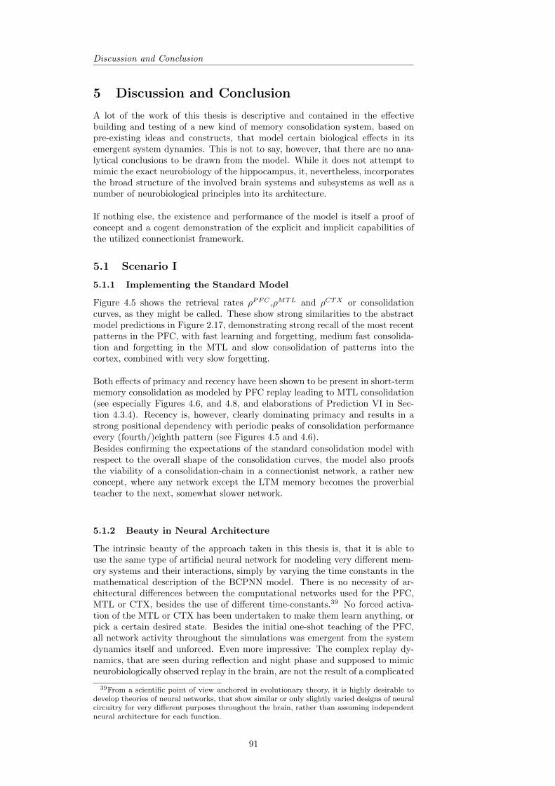
Discussion and Conclusion
5 Discussion and Conclusion
A lot of the work of this thesis is descriptive and contained in the effectivebuilding and testing of a new kind of memory consolidation system, based onpre-existing ideas and constructs, that model certain biological effects in itsemergent system dynamics. This is not to say, however, that there are no ana-lytical conclusions to be drawn from the model. While it does not attempt tomimic the exact neurobiology of the hippocampus, it, nevertheless, incorporatesthe broad structure of the involved brain systems and subsystems as well as anumber of neurobiological principles into its architecture.
If nothing else, the existence and performance of the model is itself a proof ofconcept and a cogent demonstration of the explicit and implicit capabilities ofthe utilized connectionist framework.
5.1 Scenario I
5.1.1 Implementing the Standard Model
Figure 4.5 shows the retrieval rates ρPFC ,ρMTL and ρCTX or consolidationcurves, as they might be called. These show strong similarities to the abstractmodel predictions in Figure 2.17, demonstrating strong recall of the most recentpatterns in the PFC, with fast learning and forgetting, medium fast consolida-tion and forgetting in the MTL and slow consolidation of patterns into thecortex, combined with very slow forgetting.
Both effects of primacy and recency have been shown to be present in short-termmemory consolidation as modeled by PFC replay leading to MTL consolidation(see especially Figures 4.6, and 4.8, and elaborations of Prediction VI in Sec-tion 4.3.4). Recency is, however, clearly dominating primacy and results in astrong positional dependency with periodic peaks of consolidation performanceevery (fourth/)eighth pattern (see Figures 4.5 and 4.6).Besides confirming the expectations of the standard consolidation model withrespect to the overall shape of the consolidation curves, the model also proofsthe viability of a consolidation-chain in a connectionist network, a rather newconcept, where any network except the LTM memory becomes the proverbialteacher to the next, somewhat slower network.
5.1.2 Beauty in Neural Architecture
The intrinsic beauty of the approach taken in this thesis is, that it is able touse the same type of artificial neural network for modeling very different mem-ory systems and their interactions, simply by varying the time constants in themathematical description of the BCPNN model. There is no necessity of ar-chitectural differences between the computational networks used for the PFC,MTL or CTX, besides the use of different time-constants.39 No forced activa-tion of the MTL or CTX has been undertaken to make them learn anything, orpick a certain desired state. Besides the initial one-shot teaching of the PFC,all network activity throughout the simulations was emergent from the systemdynamics itself and unforced. Even more impressive: The complex replay dy-namics, that are seen during reflection and night phase and supposed to mimicneurobiologically observed replay in the brain, are not the result of a complicated
39From a scientific point of view anchored in evolutionary theory, it is highly desirable todevelop theories of neural networks, that show similar or only slightly varied designs of neuralcircuitry for very different purposes throughout the brain, rather than assuming independentneural architecture for each function.
91

Scenario I
biologically unfounded new mechanism, but rather emergent system behaviorafter a rudimentary computational modeling of adaptation through neural andsynaptic depression with biologically reasonable time constants, as proposed byLansner and Sandberg [60]. In fact, the same adaptation time constant (160ms)is used in all memory stages, no further tuning is required to generate replay.
5.1.3 Predictability of Consolidation Performance
Despite the non-linearity and statistical complexity of the model, the largelyconfirmed predictions made beforehand in Section 3.10, demonstrated that mem-ory consolidation performance can be successfully predicted to a large extentby an understanding of the involved memory subsystems. It can be arguedthat this underscores the analytical value of separately investigating and mod-eling the different parts of the memory system (working memory, intermediatememory, long-term memory) and their related brain structures, the pre-frontalcortex, the medial temporal lobe (with the hippocampus and its surroundingcortices and gyri) as well as the neocortex, even though system memory con-solidation is a complex process involving more than one of these systems at atime.
Investigations into the observed positional dependency of consolidation oddsshowed, however, that the computational model exhibits certain counter-intuitiveproperties due to its non-linear complexity, such as the relatively lower consol-idation odds of patterns presented in the first percept of each day over thepatterns presented in the second percept of each day, despite the fact that theformer acquire more reactivations and longer reinstatement in the PFC beforethe following night phase. (See the first point of observations on page 66)
5.1.4 Why ’Unfair’ Consolidation is Natural
The analysis of positional dependence and pattern overlap clearly underscored,that the exact setup of the model phases matters, and that training patterns arenot created equal. Besides the –not unreasonable– bias towards novel (uncorre-lated) stimuli: When patterns are introduced right before a consolidation phase,they have a significant advantage over other patterns. By not implementing arandomization of the activity before each consolidation phase, we even height-ened this imbalance.
One might ask intuitively: Is the fact, that the last pattern of each percept getsone guaranteed activation during the following reflection not ’kind of unfair’?The randomizing activity reset before the onset of replay, investigated in Sec-tion 4.2 and discussed in Section 5.1.4, is not used in the general model. Thereason for this is quite simply that any introduction of outside action manipulat-ing the activity of the network during run-time, needs to be critically examinedwith respect to its biological plausibility. So let us ponder the question. Howrealistic it is, that the last percept is guaranteed to be activated first duringreflection and thus consolidates into the MTL at a significantly higher rate? Afitting real-life analogy to what happens here might be the game of memory:
Consider yourself in the position of the player, who just turned over two cards anddid not find a match. Next, your eager opponent flips over two other cards. Assum-ing he also fails to find a pair, you have just been exposed to four different perceptsfor a brief moment of time and in rapid succession, similar to a ’perception’ phase.In the pause that follows his turn, you have time to ’reflect’ on what you just saw toform a more lasting memory that can benefit you throughout the rest of the game.It is not at all unusual and completely in line with working memory theory to find,
92
Discussion and Conclusion
that you automatically start by trying to remember the card you saw/perceived last.Most people are probably not surprised to find that they can often remember thelast card best, either.
More generally, it can be argued that the last percept has a natural advantageat the onset of a ’reflection’ phase. Recency is, in fact, a well documentedeffect in working memory research [13] and this might be nothing more than a–admittedly strong– modeling of such. Given this plausible example in additionto the known effect of recency in short-term memory consolidation on the onehand, and a missing biological justification for external interventions in thenetworks activity on the other hand, we decide not to introduce any externalreset-mechanism in the general model.
5.2 Scenario II
The various experiments executed in Scenario II underscore that modulationscloser to final long-term storage are more efficient than early stage modulationsin impacting eventual long-term consolidation odds. However, modulation atany stage matters. A pattern never stored in the PFC, can not possibly aquire astable hippocampal representation, let alone become part of cortical long termmemory. Functional brain imaging experiments confirm, that successful con-solidation is highly correlated with the level of PFC activity during the initialencoding [53]. Let us not forget, that modulation serves the purpose of selectingor rejecting memories for storage as well as enhancement of important patterns.Functionally, irrelevant memories are most effectively shut out as early as pos-sible. The PFC modulation can be used to quickly reject patterns. Highlyrelevant patterns, however, are best modulated in the cortex, to maximize long-term consolidation most effectively.
It should not go unmentioned here, that a possible alternative to plasticitymodulation, namely decorrelation, exists and might be much more successfulthan any modulation. The correlation between the daily overlap of a patternand its consolidation success is high and eclipses the dynamic properties oflearning-rate modulation (see Figure 4.20). This is, however, highly related tothe size of the network.
The two isolation effects can be distinguished by their time-courseand effect on other patterns. Plasticity modulation causes retroac-tive interference and a relatively small increase in lifespan, whiledecorrelation can significantly prolong the survival of memory evenat high levels of plasticity. However, in large networks with sparseactivity random patterns will tend to have less overlap with eachother, decreasing the effect of this strength. [59, p.79]
The example in Figure 4.26 also underscores the highly non-linear dynamicsof adaptation-driven replay. These can lead to interesting situations, such asthe increased consolidation of ξ58 and ξ59, despite the fact, that they were justpartially overwritten/weakened by the strengthened encoding of the isolate ξ60.During replay, patterns compete for consolidation. In BCPNNS at least, thiscompetition generally has more than one winner (as even the most dominantpatterns become frequently depressed for considerable time after each reinstate-ment) and is fought between all patterns capable of replay. The exact oppositesituation occurs after Benzodiazepine consumption, a chemical (sometimes la-beled a date rape drug) that temporally blocks encoding of any new information.Because this means reduced consolidation competition for earlier memories, itstrongly benefits their consolidation.
93
Scenario III and Biological Comparisons
We observe increased retrieval for all patterns of a day, whenever an isolate oc-curs on that day. The described ’leaking’ of modulation to other patterns andreduced consolidation competition from older patterns, lends itself to interestingneuropsychological analogies. When plasticity is temporally increased (say bya dopaminergic plasticity modulation) during an event of increased importanceor relevance (like an emotional event), even the encoding of close by details,unrelated to the event causing the modulation, can be increased. This leadsto better consolidation and eventual long-term memory of unimportant details,just because some other important event took place as well.
5.3 Scenario III and Biological Comparisons
It can be considered a major success of this model, that it exhibits clearly bothretrograde and anterograde amnesia (RA, AA) after hippocampal lesioning (Fig-ures 4.27,4.28,4.29,4.30, and 4.31). After all, the discovery of temporally gradedRA was a driving force behind the conception of the consolidation standardmodel [39].
Even more interesting might be the relationship between RA and AA. In themodel of this thesis, AA and RA are inescapably linked. Any simulated hip-pocampal damage, that results in RA necessarily diminishes the ability of thesystem to conduct regular consolidation, thus leading to some form of AA. Themodel explicitly restricts all cortical learning to indirect learning through MTL-driven replay and there is no alternative way for the system to compensate thediminished MTL performance. In terms of the standard model parameters (seeFigure 2.16, this means, we set Sc(O) to zero. It is important to understandthat this was motivated out of the desire to measure only learning through con-solidation dynamics, not because we believe this to be an object truth.
The exact shape of the temporal gradient of RA in different kinds of lesionstudies in humans and animals has gotten a lot of attention in neuroscien-tific research and motivated theories about memory consolidation in particu-lar [38, 39, 12, 46, 4, 68, 78, 3, 49, 80]. Because scientists cannot run controlledexperiments with human hippocampal lesioning, we rely on accidents but aplethora of animal lesion studies (mostly rats and more rarely monkeys, butalso mice, rabbits and birds) have contributed to our understanding of the ef-fects of hippocampal lesioning on memory. An interesting panel of RA gradients(to be compared against the RA gradient of this thesis in Figure 4.29) from var-ious lesion studies can be found in a much cited 1995 psychological review paperby J.L. McClelland, B.L. McNaughton, and R.C. O’Reilly [38] (see Figure 5.1).
A quantitative comparison of the RA gradients and extent of AA in this modelwith biological data is questionable and difficult. Nevertheless, the importantlesson to take away is the overall shape of the RA-gradients in Figures 4.29and 5.1, which are virtually identical, showing that this computational modelproduces memory effects similar to biological studies.
But before we congratulate ourselves too hard, we need to look further: Ina comprehensive review of both human and animal studies [49], Nadel andMoscovitch concluded that the considerable amount of conflicting data on theshape of RA gradients after hippocampal lesioning and their relationship to AAconstitutes a serious problem within the standard model. There is contradictoryevidence as to how predictable the temporal gradient of RA is and whether theapplicability of Ribbot’s Law needs to be restricted with respect to the nature,extent, or overall types of memory it being applied to.
While most studies show a strong link between RA and AA, certain other cases
94

Discussion and Conclusion
Figure 5.1: Panels a-c: Behavioral responses of animals receiving extensive hippocam-pal system lesions (circles) or control lesions (squares) as a function of the numbersof days elapsing between exposure to the relevant experiences and the occurrence ofthe lesion. Bars surrounding each data point indicate the standard error. Panel ashows the percentage choice of a specific sample food (out of two alternatives) byrats exposed to a conspecific that had eaten the sample food. Panel b shows fear(freezing) behavior shown by rats when returned to an environment in which theyhad experienced paired presentations of tones and footshock. Panel c shows choicesof reinforced objects by monkeys exposed to 14 training trials with each of 20 objectpairs. Panel d: Recall by depressed human participants of details of TV shows aireddifferent numbers of years before the time of test after electroconvulsive treatment[circles] or just before treatment [squares]. Here years have been translated into daysto allow comparison with the results from the animal studies. The curves shown ineach panel are based on a simple model discussed in the text and depicted in Figure14 (with the parameters shown in Table 1). Note. Data in Panel a are from ’An-terograde and Retrograde Amnesia in Rats With Dorsal Hippocampal or DorsomedialThalamic Lesions,’ by G. Winocur, 1990, Behavioral Brain Research, 38, p.149. Datain Panel b are from ’Modality-Specific Retrograde Amnesia of Fear,’ by J. J. Kim andM. S. Fanselow, 1992, Science, 256, p.676. Data in Panel c are from ’The PrimateHippocampal Formation: Evidence for a Time-Limited Role in Memory Storage,’ byS. Zola-Morgan and L. R. Squire, 1990, Science, 250, p.289. Data in Panel d are from’Memory and Amnesia: Resistance to Disruption Develops for Years after Learning,’by L. R. Squire and N. Cohen, 1979, Behavioral and Neural Biology, 25, p.118.
[38]
show very extensive, flat RA (very much unlike the gradients above), often withrespect to autobiographical memory in humans (and spatial memory in rats),that is not necessarily accompanied by a similar degree of AA (e.g.[24]). Here itseems, that the hippocampus is required for all stages of learning and remem-bering. Some review papers [49] call explicit attention to the inadequacy of thestandard model of consolidation in dealing with cases of disassociated AA and
95

Scenario IV
RA. In cases of flat RA for 20, or 30 years of autobiographical memories, itseems unreasonable to proclaim that consolidation processes are in fact at workbut require decades to complete. It is safe to say that this should be rejected asan attempt to uphold a standing theory in light of conflicting data by makingunreasonable assumptions. In biological studies, the upper limit of AA causedby increasing damage is generally reached sooner than the upper limit for RA.This has been shown in this model to a small extent as well: Upon increasinglesions, the adaptation dynamics and the consolidation that relies on it, breaksdown somewhat faster than the MTL retrieval rate of already stored patterns.When RA and AA become dissimilar in biological lesion studies, then it is usu-ally the degree of rather flat RA that eclipses the degree of AA. Strong AA byitself without any RA is not observed in lesion studies40. In light of these facts,the simple model of this thesis should be considered a partial success on the roadto a necessarily more complex computational model of memory consolidation.
5.4 Scenario IV
The fact that reduced sleep length progressively worsens learning success cannot be surprising. After all, the setup of the model was such that all learning inthe cortex is accomplished exclusively through a sleep-dependent, replay-drivenconsolidation mechanism. What is more interesting, the model exhibits an op-timal night length and shows how over-sleeping can actually gradually decreaseconsolidation performance as well. This is a result that parallels other com-putational attempts of mimicking sleep-consolidation (see Section 5.7) and isgenerally an effect of overwriting, caused by the limited capacity of the corticalnetwork. Given the enormous size and capacity of the biological neocortex incomparison to the small fields of CA1 and CA3 neurons in the hippocampus(only a few million neurons), we can hypothesize that the reason for not observ-ing this in biological studies is an expression of relative scale.
The model also repeatedly proofed (in earlier Scenarios) the common theory,that interference is bad for consolidation, which should be a general property ofevery probability-based attractor neural network.
One of the more interesting aspects is how the biological discussion on whethersleep is permissive to consolidation or actively engaged in consolidation is re-flected in this model. In a comprehensive review [14], sleep researchers laid outthese two alternatives (there called Hypothesis three and four):
• III. Either sleep creates conditions conducive to memory consolidation,but plays no other or unique role in the consolidation process, or
• IV. Unique properties of sleep are directly involved in memory consolida-tion processes.
With behavioral measures alone, it is difficult to distinguish whethersleep is enabling consolidation to occur, as in hypothesis three, orwhether sleep activates unique neurobiological processes that playa direct role in consolidation, as predicted by hypothesis four. Thedistinction rests on knowledge of the precise physiologic markers ofconsolidation, interference and their relationship to sleep. [14]
40But of course it is entirely possible to achieve some extent of AA without RA by othermeans, such as sleep deprivation or drugs like benzodiazepin. Benzodiazepin can, in fact,cause complete AA, blocking the encoding of new information, while at the same time stronglybenefiting the consolidation of pre-existent memories. This also underscores the competitivenature of consolidation processes.
96

Discussion and Conclusion
The model of this thesis is flexible enough for dealing with any of these possi-bilities:
• If biological data were to confirm the first hypothesis, the model couldeasily be set up such that the adaptation projections are always active,but new input to a memory stage are introduced with a high gain. Thiswill lead to slightly altered dynamics, where the stream of new sensory-input will override adaptation-driven replay dynamics temporarily (like inwake activity or unreflective behavior). In such a model, sleep (shuttingdown new input) will be conducive to memory consolidation because itwill allow the adaptation driven replay to determine the system dynamicsand drive consolidation.
• On the other hand, the thesis model can be made to reflect the laterhypothesis as well. When we turn off adaptation driven replay of theMTL during the day phase (as was done for the Scenarios investigatedin this thesis) then we might call the activation of said replay a special,active form of sleep-dependent memory consolidation.
97

Conclusion
5.5 Conclusion
Overall, the model achieved what it set out to do, which was to build an extendedimplementation of the memory consolidation standard model using BCPNNs.Due to its three-stage architecture, it features the entire consolidation processfrom one-shot learning (sensory memory ) capability to very stable corticalmemory engrams and many other features one would expect from such an im-plementation such as competitive consolidation, effects of primacy and recencyin short-term consolidation as well as typical amnesia effects after simulatedhippocampal lesions. With respect to the latter, we conclude that the modelreproduces graded RA which was one of the main driving forces behind thedevelopment of the memory consolidation standard model. As such, this com-putational model is a rather successful implementation of said model. In theopinion of the author, the contradictory biological evidence with respect to thelink between RA and AA clearly points out a vulnerability in the memory con-solidation standard model. It underscores the necessity of testing variationsof the standard models (such as considering reconsolidation processes [77, 3],schema theory [71], multiple trace theory [49] or a kind of trace-link system [46]),some of which have already been shown to deal with certain known inconsis-tencies of the standard model. Irrespective of that, the impressive success ofthe standard models in explaining temporally graded RA, AA and the overalldynamics of memory consolidation even in conjunction with plasticity modula-tions, underscores its value. The fact that all of this can be generated from avery limited mathematical model by choosing a few appropriate time-constantsonly adds to this. To the authors knowledge, this thesis is the first, to showthe viability of a three-stage consolidation chain, driven by autonomous replayin a connectionist memory model and thus expands the architectural optionsavailable to researchers today.
5.6 Problems and Limitations
The model is strictly qualitative. For continued progress in modeling of the hu-man brain, it will become inevitably necessary to develop appropriately scaledquantitative models –tied to experimental data– as well.41 Only then can quan-titative predictions be made from those models to be compared against neu-robiological experiments to allow for probabilistic falsification of qualitativelyreasonable but quantitatively untested models. The model laid out in this thesishas a high degree of flexibility and as a first step it is certainly possible to movethe range of parameters (such as the length and number of phases and patterns)closer to biologically relevant quantities. Whether the system can then also re-tain its qualitative behavior remains to be seen.
Obviously the absolute size of the neural networks simulated are tiny in compar-ison to the real brain regions involved and despite attempts to mimic biology,this model is a far cry from the complexity of real neural activity. However,this thesis is not concerned with life-like simulations. Rather the focus is set oninvestigating the dynamics of memory consolidation in a model that builds onaccepted theories about systems neurobiology and successfully shows, that thesame general architecture of BCPNNs with adaptation projections can be usedto model all three assumed memory stages, from sensory memory to long-termmemory, by only changing the time-constants of the model.
Some critics may argue, that the use of a Hebbian rules is problematic. Firstof all, we know that the learning rules of real spiking neural networks are morecomplex than that (spike-time dependent plasticity), however as this is not a
41The ’Neurological Prediction Challenge’ issued by UC Berkley is an interesting exampleof this approach.
98

Discussion and Conclusion
spiking network simulation this seems to be a tricky argument to make. Furthercritics may argue, that Hebbian depression is problematic because, for an exam-ple, it means that memories will not decay by sheer passage of time. They aremistaken on two accounts: First, many successful neuropsychological memorymodels such as TRBS [50] indicate that it is not time itself, but rather distrac-tions/secondary activations that cause memory decay. So the observation thattime itself decays neurological memory may be a flawed conclusion, based on ourinability to measure every distractor in a given time-interval and its effects 42
Secondly, the model proposed in this thesis is indeed capable of simulating this(seemingly) time-based decay, if augmented with a random noise-backgroundactivity. BCPNNs have many advantages over other types of neural networks,chief among them, that they are derived directly from Bayes Theorem (so theiractivity can be directly interpreted as probability distributions) and that theyare easily capable of modeling very different types of memories and generaterobust replay dynamics with only minor modifications. One of their biggestdrawbacks is, the intractability of mathematical analysis due to the use of non-linear functions (log) and the normalization of activity. Using random patternswith consequently random degrees of overlap only complicates this problem fur-ther, making this thesis an exercise in experimental mathematics, rather thantheorem proof deduction.
Clearly, the dynamics of BCPNNs and interconnected networks of these, are notyet understood completely. The discovery of the unstable mode in ScenarioI andthe need for outlier detection as well as the peculiar positional dependencies (seePFC Replay in Figure 3.7) should be a warning to us, even if preliminary in-vestigations showed that this unstable mode can be eliminated by noise, moreextreme adaptation gains or by scaling up the system, as this will reduce thedegree of correlation between random patterns.
Last but not least, we have already seen the standard model repeatedly un-der attack from incompatible biological observations (see Section 5.3). It isnot unlikely, that neurobiological research will necessitate a change of the cur-rent model, even though no new, generally accepted alternative to the standardmodel has been found yet. Given this lack of a framework, more in line with neu-robiological data, however, this computational implementation remains relevantin the field of memory research as is.
5.7 Comparison with other Computational Models
The model of this thesis clearly motivates a comparison with other computa-tional models of memory consolidation. Many attempts have been made toinstantiate the standard model and variations of it in connectionist models ofsome sort. These are often difficult to compare as they vary not only in struc-ture, scale and parameters, but also their set goals, as well as level of detailand exact algorithmic implementation. The model of this thesis is probablybest contrasted with models that forgo an attempt to mimic in-depth molec-ular neurophysiology (such as modeling ion channels) and aim at a model ofsystem consolidation instead. For direct comparison, we are also interested inpapers involving memory on multiple time-scales, reinstatement of some sort,and the use of auto-associative networks for pattern storage. Some papers, suchas the hippocampal-cortical model by Pan and Tsukada [54], which uses a singlelayer network for the hippocampus and achieves interesting results for sequen-tial learning might be very interesting and definitely worth reading, but do notmerit a direct discussion here for the reasons stated above.
42On a larger time-scale of several days, degradation of individual synaptic receptor proteinshas been observed in vivo [65] and might be a more relevant argument.
99

Comparison with other Computational Models
Model This Thesis TraceLink [46] SRR model [77]
Architecture 3-stage 2-stage 2-stageANN Class modified BCPNN modified Hopfield modified Hopfield
60 unitsShort-term 10% activity — not implemented — — not implemented —memory full connectivity
τPFCL = 5
MTL/ 120 units 36 units 100 unitsHippocampus/ 10% activity 28% activity 50% activityLink System/ full connectivity 50% connectivity full connectivity
τMTLL = 300 τLink
L = 25 τHippocampalL = 1000
MTL full connectivity 50% connectivity strong-to- plastic functionally integrated fixedCTX τMTL2CTX
L = 20 with link system 1-to-1 mapping
240 units 400 units 50 unitsLong-term 10% activity 5% activity 50% activitymemory/ random overlap artificially decorrelated random overlapCortical full connectivity 20% connectivity full connectivitysystem τCTX
L = 18.000 τTraceL = 500 τL = 5000(by time scaling)
1-shot learning 10 iterations/patterns 100 iterationsInitial in PFC hippocampal and for sequential, cyclictraining no CTX training cortical training MTL-training of
8patterns/day 1pattern/day 5 patterns
Simulationcycles 10days 15days 1day
autonomous, 3 noise bursts 1 noise burst everyadaptation-driven followed by 40 iterations for
Replay/ replay with full convergence and 5000 iterations withConsolidation continuous 5 iterations learning continued learningdynamics learning during convergence
of projectedpatterns added 75% unlearning added weight decay
Table 5.1: Exemplary comparison of parameters and architecture in three differentmodels
5.7.1 Murre: TraceLink
One of the more interesting alternative models might be the TraceLink model [46]by J.M.J. Murre. First of all, it achieves what other straight-forward instantia-tions of the standard model have done before: To build a system with memoryon different time-scales, capable of executing gradual memory consolidation andexhibits a Ribot gradient of RA after simulated hippocampal lesioning. How-ever, the model sticks out, by focusing on cases of disassociation between AAand RA after lesioning.
Featuring a slow learning cortical trace system and a faster learning, hippocam-pal link system, as well as a modulatory system representative of the basalforebrain, it does not look very dissimilar to the model of this thesis at first, butthere are a few notable systemic differences to the model of this thesis. Proba-bly most significant is the generally lower connectivity. It implements only verylimited (clustered) cortical connectivity in an effort to minimize connectivityvolume. This is motivated by neurobiological observations of limited connectiv-ity which were disregarded in the model of this thesis. In TraceLink, connectionsbetween cortical elements of a trace are not just initially weak and learned slowlyafter many reactivations, referred to as co-activations. They, in fact, often onlycome into existence during consolidation (see Figure 5.2). TraceLink uses aconsolidation strategy emergent from the structure of the model architecturebut still requires noise to jump between attractors that are to be reinforced (An
100
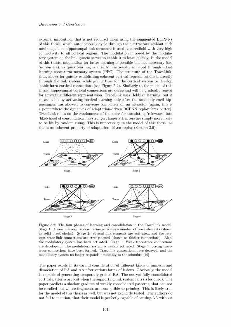
Discussion and Conclusion
external imposition, that is not required when using the augmented BCPNNsof this thesis, which autonomously cycle through their attractors without suchmethods). The hippocampal link structure is used as a scaffold with very highconnectivity to all cortical regions. The modulation imposed by the modula-tory system on the link system serves to enable it to learn quickly. In the modelof this thesis, modulation for faster learning is possible but not necessary (seeSection 4.4), as quick learning is already functionally achieved through a fastlearning short-term memory system (PFC). The structure of the TraceLink,thus, allows for quickly establishing coherent cortical representations indirectlythrough the link system, while giving time for the cortical system to developstable intra-cortical connections (see Figure 5.2). Similarly to the model of thisthesis, hippocampal-cortical connections are dense and will be gradually reusedfor activating different representation. TraceLink uses Hebbian learning, but itcheats a bit by activating cortical learning only after the randomly cued hip-pocampus was allowed to converge completely on an attractor (again, this isa point where the dynamics of adaptation-driven BCPNN replay fares better).TraceLink relies on the randomness of the noise for translating ’relevance’ into’likelyhood of consolidation’, as stronger, larger attractors are simply more likelyto be hit by random cuing. This is unnecessary in the model of this thesis, asthis is an inherent property of adaptation-driven replay (Section 3.9).
Figure 5.2: The four phases of learning and consolidation in the TraceLink model.Stage 1: A new memory representation activates a number of trace elements (shownas solid black circles). Stage 2: Several link elements are activated, and the rele-vant trace-link connections are strengthened (shown as thicker connections). Also,the modulatory system has been activated. Stage 3: Weak trace-trace connectionsare developing. The modulatory system is weakly activated. Stage 4: Strong trace-trace connections have been formed. Trace-link connections have decayed, and themodulatory system no longer responds noticeably to the stimulus. [46]
The paper excels in its careful consideration of different kinds of amnesia anddissociation of RA and AA after various forms of lesions. Obviously, the modelis capable of generating temporally graded RA. The not-yet fully consolidatedcortical patterns are lost when the supporting link system fails (is lesioned). Thepaper predicts a shadow gradient of weakly consolidated patterns, that can notbe recalled but whose fragments are susceptible to priming. This is likely truefor the model of this thesis as well, but was not explicitly tested. The authors donot fail to mention, that their model is perfectly capable of causing AA without
101

Comparison with other Computational Models
RA when the modulatory system fails. A similar effect could be achieved inthe model of this thesis by damaging the connectivity between the PFC andthe MTL (not tested in this thesis). For this effect to occur after hippocampallesioning, as has been observed, the authors require the modulatory system tobe located near, or be part of the hippocampus. By varying the extent of thelesions in the modulatory system and the link system, they can achieve AA withvarying degrees of RA. In the next step of trying to explain how their modelcould also show isolated RA with a gradient, they explain how the hippocampusmight be overwritten with neural noise, that essentially deletes all hippocampalweights but preserves the full functionality of the system to learn and consoli-date new patterns. This would be the result of some speculative phenomenon,whereby the modulatory basal forebrain would be continuously and uniformlyactive. Their explanation for isolated flat RA after cortical lesions, on the otherhand, is more straight-forward: After a lesion to the cortical knowledge base, thememories stored there would be lost (flat RA) without general AA. Among theirmost interesting speculations is the idea of a rare inverse Ribot gradient. Whencortical connectivity is disrupted (rather than destroying its nodes) all repre-sentations become reliant on the hippocampal link system (that may or maynot have forgotten or since reused the necessary connections). Initial episodiclearning continues as usual, but memory consolidation becomes impossible. Theresult would be a strange case of severe AA, and RA with an inverted forgettingcurve that shows steeper than usual forgetting because all memories now rely onthe linking hippocampus and are thus forgotten faster than usual. In supportof their idea, the authors cite a few rare cases where this inverted gradient hassupposedly been observed.
5.7.2 Walker, Russo: Consolidation and Forgetting during sleep
With respect to our variation of the sleep length in Scenario IV, this thesis pro-vokes a comparison with a 2004 paper by Walker and Russo [75]. A lot of themore theoretical background for this paper can be found in a paper by Walkerand Stickgold from the same year [74]). Because the authors want to use aHopfield network, they have to deal with the problem of catastrophic forget-ting (CF). They take the issue head on and discuss various proposed ways of’unlearning’ to keep Hopfield networks a viable ANN for memory studies. Wealready talked about the un-biological nature of CF and how the BCPNN, usedin this thesis, inherently avoids this issue, so no extra measures of unlearningneed to be taken to avoid CF in BCPNNs (see Section 2.6). Despite using aHopfield network, they find an interesting solution to establish viable memoryconsolidation in this framework. After learning and cutting all sensory input atthe beginning of a sleep phase, they cue the system with random noise bursts.They show that high amplitude, low frequency noise will strengthen the at-tractors in their network of 150 units (a consolidation effect). They also varythe night length and similarly to this thesis, they find an optimal night lengthfor consolidation. Because they measure retrieval error rather than a positiveretrieval-rate, their curve looks U-shaped instead of a bell-curve. The overallshape (flipped upside-down) is however very similar to the results of ScenarioIV (compare Figures 5.3 and 4.32).In contrast to this thesis, their model does not distinguish different types ofmemory (short-term, intermediate, long-term) systemically. Because of that,they have to find some other way to manage bridging the gap in timescale be-tween fast episodic learning and slow long-term consolidated memories. Thisis done by keeping two separate sets of weights, one with a high learning rate(α = 0.01) and one with a 100-times slower learning rate (α = 0.0001). Froma biological point of view, these double weights for each connection might bequestionable, but it does achieve the desired result. Walker and Russo also donot limit all learning to consolidation, so Figure 5.3 shows a certain positive
102
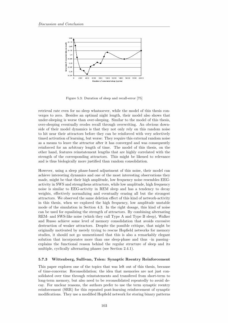
Discussion and Conclusion
Figure 5.3: Duration of sleep and recall-error [75]
retrieval rate even for no sleep whatsoever, while the model of this thesis con-verges to zero. Besides an optimal night length, their model also shows thatunder-sleeping is worse than over-sleeping. Similar to the model of this thesis,over-sleeping eventually erodes recall through overwriting. An obvious down-side of their model dynamics is that they not only rely on this random noiseto hit near their attractors before they can be reinforced with very selectivelytimed activation of learning, but worse: They require this external random noiseas a means to leave the attractor after it has converged and was consequentlyreinforced for an arbitrary length of time. The model of this thesis, on theother hand, features reinstatement lengths that are highly correlated with thestrength of the corresponding attractors. This might be likened to relevanceand is thus biologically more justified than random consolidation.
However, using a sleep phase-based adjustment of this noise, their model canachieve interesting dynamics and one of the most interesting observations theymade, might be that their high amplitude, low frequency noise resembles EEG-activity in SWS and strengthens attractors, while low amplitude, high frequencynoise is similar to EEG-activity in REM sleep and has a tendency to decayweights, effectively normalizing and eventually erasing all but the strongestattractors. We observed the same deletion effect of this kind of network-activityin this thesis, when we explored the high frequency, low amplitude unstablemode of the simulation in Section 4.3. In the right dosage, this kind of noisecan be used for equalizing the strength of attractors. By combining alternatingREM- and SWS-like noise (which they call Type A and Type B sleep), Walkerand Russo achieve some level of memory consolidation that avoids excessivedestruction of weaker attractors. Despite the possible critique, that might beoriginally motivated by merely trying to rescue Hopfield networks for memorystudies, it should not go unmentioned that this is also a remarkably elegantsolution that incorporates more than one sleep-phase and thus –in passing–explains the functional reason behind the regular structure of sleep and itsmultiple, cyclically alternating phases (see Section 2.4.1).
5.7.3 Wittenberg, Sullivan, Tsien: Synaptic Reentry Reinforcement
This paper explores one of the topics that was left out of this thesis, becauseof time-concerns: Reconsolidation; the idea that memories are not just con-solidated over time through reinstatements and transfered from short-term tolong-term memory, but also need to be reconsolidated repeatedly to avoid de-cay. For unclear reasons, the authors prefer to use the term synaptic reentryreinforcement (SRR) for this repeated post-learning reinforcement of synapticmodifications. They use a modified Hopfield network for storing binary patterns
103

Comparison with other Computational Models
with Hebbian learning and an added proportional decay term. They justify thisdecay by neurophysiological data, stating that ’individual synaptic receptor pro-teins are known to be degraded over the course of days’. Long-term memoryconsolidation is known to continue for weeks and consequently, single LTP-likemolecular cascades are deemed inadequate because of their potentially shortertime-scale. The authors consequently demand a mechanism for repeated re-initiation of NMDA receptor-gated cascades. Like so many others before them,the authors then go on to use random noise cuing (noise bursts of constantfrequency) for facilitating reinstatements after initial learning. The small, butimportant difference is that they explore this method of generating reactivations(which they call SRR-Events) not just for consolidating them into a slower learn-ing network (they try this later too), but then also for the purpose of keepingtheir now decaying memories alive. Obviously, these reconsolidation dynamicsare competitive as well, so they find that over time only the strongest patternsurvives (lack of normalization). After clarifying that [...]’it is not clear thatthis is the same method used by the brain to reactivate memory traces’, theyextend the system to a hippocampal-cortical system. The cortical network isset to run five times slower than the hippocampal network and for unclear rea-sons, they choose the cortical network to be two times smaller.. They use aone-to-one mapping between hippocampal and cortical neurons with fixed con-nection strength. Note, that this was an approach tested by Liljencrantz [34]in BCPNNs, deemed functionally suboptimal, lacking biological support andwas consequently replaced in this thesis by a full dynamic connectivity, whichallows for dynamically associating any two representations on the hippocampaland cortical level. The SRR-model implements partial cortical learning duringthe initial hippocampal training phase (this thesis restricted it to consolidation-based learning) but shows how the cortical trace really gathers its strength(measured as speed of convergence) as a function of hippocampally induced re-activations (called SRR-Events). This relationship can easily be compared withthe number of reactivations in the MTL (NPRMTL) and the correspondingcortical retrieval rate ρCTX in the model of this thesis, which found a Pearsoncorrelation coefficient of r=0.74 (see Table 4.1 and Figures 4.18) and a similarshape (see side-by-side comparisson in Figure 5.4).
Figure 5.4: Left: Relationship between the number of pattern reactivations in theMTL (NPRMTL) and cortical retrieval rate (ρCTX) of the corresponding pattern inthe model of this thesis (see Section 4.3.2), Right: Relationship between the number ofsynaptic reentry reinforcement events and cortical retrieval rate in the SRR-Model [77]
From this point of view, replay serves a double purpose:
• First, it helps to keep current attractors alive in the presence of decay andnoise.
• Second, it drives reinstatement of memory traces on higher stages andthus enables progressive long-term memory consolidation.
In the end, the authors speculate about abnormal SRR as the cause for certain
104
Discussion and Conclusion
aspects of epilepsy and schizophrenia.
In conclusion, if reconsolidation is warranted by molecular analysis and it inte-grates so nicely with aspects of long-term consolidation, why should we not beinspired to bridge the gap between memory consolidation on the molecular andnetwork level in future models this way?
5.8 Future Work
Looking at the development of current models of consolidation and their varyingsuccess in explaining consolidation data, we might argue that it is about timeto start integrating differing models rather than trying to generate more andmore contrasting models with intricately modeled details. Obviously, the fieldcontinues to depend on further neurophysiological evidence, especially from am-nesia studies. In the opinion of the author, the modified BCPNN framework cancontribute to the unification of models, as it can easily be integrated with manymodels on an algorithmic level, often without changing their proposed systemicarchitecture. This way, it quickly replaces other, more crude forms of replay-generation (such as random noise cuing in abundantly used Hopfield networks)by use of its inherent properties, and since its network activity reflects proba-bility distributions, and its logarithmic weights model conditional probability,activity and weights become directly susceptible to probabilistic arguments.
A lot of aesthetic work can be done by tuning the system of this thesis to bio-logically more reasonable parameters. This especially relates to time-constants,the number of patterns, phases and the durations thereof. Given the manytrade-offs between parameters, it is likely that a much more plausible set ofparameters exists.
A related, highly interesting aspect not experimented upon in greater depth(but observed nevertheless) is, that the sensitivity with respect to modulation(see Scenario II) can be much higher if the system is tuned closer to the con-solidation edge. What do we mean by this? When a memory system featuresdecorrelated patterns or large scale (reduced overlap), the amount of consoli-dation time required for retrieval on the next stage can be known much moreprecisely due to the eliminated impact of overlaps on reinstatement lengths.Consequently, the memory system can be tuned (by changing the gains of as-sociations and adaptations) to have the average consolidation time very closeto this consolidation-edge. In our implementation with random patterns of lowdimensionality, this edge is blurred (e.g. see the steepness of the curve for therelationship between TPRLMTL and ρCTX in Figure 4.18) and consequently itis hard to find a good set of parameters.
The current model can be extended in many possible direction, ranging frommodeling the forward pass for creating associated patterns on different stages(instead of using random patterns), using multiple traces with partial overlapas an instantiation of the multiple trace theory [49] and implementing recon-solidation mechanics [3] or learning of sequences to spiking network simulationsand other in-depth models. Especially with respect to reconsolidation and thesynaptic reentry model [77], we should add that integration of some level ofreconsolidation mechanics is both feasible and easy to accomplish within thecurrent model. In fact, we only need to let the networks stay plastic duringreplay. This way, patterns naturally decay outside of regular learning but are re-peatedly reinforced through the converging quasi-attractors. Even better: Thiscan be accomplished autonomously, without external bursts of cuing noise, orrepeated network reinitialization but will probably require some tuning to find
105
Personal Reflection
the right balance between decay and reconsolidation.
5.9 Personal Reflection
This thesis consumed the better part of a year and probably changed my ownacademic orientation by quite a bit. Having started as nothing more than a well-educated systems engineer with a personal fascination for neurobiology and arti-ficial intelligence, I was initially struck by the rainforrest of confusing complexityin neuroscientific research. Being an autodidact by nature, I carefully educatedmyself on basic neuroscience and gradually started narrowing my field of viewon the topic of memory consolidation. However, I still found that completeunderstanding of relevant concepts (such as LTP) required reading referencesand references of references. After having read about a hundred papers over thecourse of a few months i personally found the explanations of basic conceptsand their origins to be often lacking motivation and comprehensiveness. Thiseventually became my own reason for writing a rather comprehensive basicschapter, unusually large for a masters thesis project maybe. It served the orga-nization my own conception during writing, as well as it will, hopefully, servethe potential reader of my thesis, that might not have a neuroscience and acomputerscience degree.
Working with the recurrent BCPNN framework, conceived and intelligently ex-panded upon by Lansner and Sandberg, was incredibly rewarding. In a moststartling moment, I found out that Anders Sandberg (whom I have never met)was actually the same guys, whose great transhumanist blog I had been follow-ing for about a year with great enthusiasm, prior to starting my thesis work.I especially liked, that while the activity in modified Hopfield networks can becompletely cryptic to read, almost everything about BCPNNs has an intuitive,probabilistic explanation. My personal devotion to neuroscience was originallyinspired by Jeff Hawkins and his memory-prediction framework [22], which dealsextensively with the question of how we know almost everything through prob-abilistic computing. With this personal interest in memory research and mybackground in systems engineering, this thesis felt more than fitting.
The computational costs and required runtime were probably the only annoyingparts of my work. By insisting on random patterns and thus random patternoverlaps, large parameter spaces and extensive testing as well as near-certainaverages, many results required hundreds if not thousands of simulation runsto generate good data resolution. Trying to peer into the inner workings ofthe model required cataloging and analyzing piles of network activity data. TheMATLAB environment I had soon built for running the model and data analysis,proofed to be versatile and easy to debug. But as MATLAB is not exactly a fastrunning computer language for iterative simulations, it slowed down my workwhenever i had less than half a dozend processor cores working for me. Thegenerosity of my friends in donating some computing time eventually turnedthe tide and even though there is always more to do in a large, complex modellike this one, the work feels reasonably complete now.
106

References
References
[1] Abbott, L.F., Varela, J.A., Sen, K. and Nelson, S.B. (1997) Synaptic de-pression and cortical gain control, Science 275(5297):220-4.
[2] Agnati, L.F., Fuxe, K., Nicholson, C. and Sykova, E. (2010) Vol-ume Transmission Revisited, Progress in Brain Research, Elsevier, ISBN9780444503145
[3] lberini, C.M. (2005), Mechanisms of memory stabilization: are consolida-tion and reconsolidation similar or distinct processes?, TRENDS in Neu-rosciences, 28:51-56.
[4] Alvarez, P. and Squire, L.R. (1994), Memory consolidation and the medialtemporal lobe: A simple network model, PNAS Neurobiology, 91:7041-7045.
[5] Anastassiou, C.A., Perin, R., Markram, H. and Koch, C. (2011), Ephapticcoupling of cortical neurons, Nature Neuroscience 14 (2): 217
[6] Baddeley, A.D. and Hitch, G. (1974), Working memory. In G.H. Bower(Ed.), The psychology of learning and motivation: Advances in researchand theory (Vol. 8, pp. 47–89), New York: Academic Press.
[7] Bliss, T.V.P., Gardner-Medwin, A. R. and Lømo, T. (1973) Synaptic Plas-ticity in the Hippocampal Formation. G. B. Ansell and P. B. Bradley (eds.),Macromolecules and Behavior, London: MacMillan, pp. 193–203.
[8] Cohen, N.J. and Squire, L.R. (1980), Preserved lerning and retention ofpattern-analysing skill in amnesia: dissociation of knowing how and know-ing that, Science 210: 207-210.
[9] Cooke, S.F., Bliss, T.V. (2006). Plasticity in the human central nervoussystem Brain 129 (Pt 7): 1659–73.
[10] Craver, C.F. (2003), The Making of a Memory Mechanism, Journal of theHistory of Biology, 36:153-195.
[11] Dudai, Y. (1989), The Neurobiology of Memory: Concepts, Findings,Trends, Oxford University Press.
[12] Dudai, Y. (2004), The neurobiology of consolidation, or how stable is theengram?.
[13] Ebbinghaus, H. (1885) Uber das Gedachtnis: Untersuchungen zur exper-imentellen Psychologie Unchanged republished original german text from1885. Darmstadt, Wissenschaftliche Buchgesellschaft, 1992. ISBN 3-534-05255-2
[14] Ellenbogen, J.M., Payne, J.D. and Stickgold, R. (2006), The role of sleepin declarative memory consolidation: passive, permissive, active or none?,Current Opinion in Neurobiology, 16:716-722.
[15] Ellenbogen, J.M., Hulbert, J.C., Stickgold, R., Dinges, D.F., Thompson-Schill, S.L. (2006) Interfering with theories of sleep and memory: sleep,declarative memory, and associative interference, Curr Biol 2006, 16:1290-1294.
[16] Fausett, L. (1993), Fundamentals of Neural Networks: Architecture Algo-rithms and Applications, Prentice Hall, 1st edition.
[17] Fransen, E. and Lansner, A. (1995) Low spiking rates in population ofmutually exciting pyramidal cells Network, 6(2):271-288.
107

References
[18] Freedman, M. and Oscar-Berman, M. (1986) Bilateral frontal lobe diseaseand selective delayed response deficits in humans., Behavioral Neuroscience,Vol 100(3), Jun 1986, 337-342, 433-435.
[19] Funahashi, S., Bruce, C.J. and Goldman-Rakic P. S. (1989) Mnemoniccoding of visual space in the monkey’s dorsolateral prefrontal cortex, Journalof Neurophysiology 61(2):331:349
[20] Gais, S., Lucas, B., Born, J. (2006) Sleep after learning aids memory recall.,Learn Mem 2006, 13:259-262.
[21] Goodwin, D.W., Crane. F.B., Guze, S.B. (1969) Alcoholic ’blackouts’: Areview and clinical study of 100 alcoholics American Journal of Psychiatry126:191-198.
[22] Hawkins, J. and Blakeslee, S. (2005). On intelligence St. Martin’s Griffin;1st ed., ISBN 9780805078534
[23] Hebb, D. O. (1949). Organization of Behavior: A Neuropsychological The-ory. New York: John Wiley. ISBN 0-471-36727-3.
[24] Hokkanen, L., Launes, J., Vataja, R., Valanne, L., et al. (1995) Isolatedretrograde amnesia for autobiographical material associated with acute lefttemporal lobe encephalitis, Psychological Medicine: A Journal of Researchin Psychiatry and the Allied Sciences, Vol 25(1), Jan 1995, 203-208.
[25] Holst, A. (1997), The Use of a Bayesian Neural Network Model for Clas-sification tasks, Disseration, Department of Numerical Analysis and Com-puting Science, Royal Institute of Technology, Stockholm.
[26] Jenkins, J.G. and Dallenbeck, K.M. (1924) Obliviscence during sleep andwaking.,Am J Psychol 1924, 35:605-612
[27] Johansson, C., Raicevic, P. and Lansner, A. (2003), Reinforcement Learn-ing based on a Bayesian Confidence Propagating Neural Network, Depart-ment of Numerical Analysis and Computer Science, Royal Institute of Tech-nology, Stockholm.
[28] Johansson ,C. and Lansner, A. (2004), BCPNN Implemented with Fixed-Point Arithmetic, Department of Numerical Analysis and Computer Sci-ence, Royal Institute of Technology, Stockholm.
[29] Kandel, E.R., Schwartz, J.H. and Jessell, T.M. (2000), Principles of Neu-ral Science Fourth Edition. United State of America, McGraw-Hill. ISBN0838577016.
[30] Koch, C. (2004), The Quest for Consciousness: A Neurobiolological Ap-proach, Roberts & Company .
[31] Johansson, C. and Lansner, A. (2007). Towards cortex sized artificial neu-ral systems Neural Netw 20 (1): 48–61. doi:10.1016/j.neunet.2006.05.029.PMID 16860539.
[32] Kotter, R. (1994). Postsynaptic integration of glutamatergic and dopamin-ergic signals in the striatum Progress in Neurobiology 44:2 p163-196.
[33] Lansner, A. and Ekeberg, O. (1989) A one-layer feedback artificial neuralnetwork with a bayesian learning rule, Int. J. Neural Systems, 1(1):77-87.
[34] Liljencrantz, A. (2003), Memory Consolidation in Artificial Neural Net-works, Department of Numerical Analysis and Computer Science, RoyalInstitute of Technology, Stockholm.
108

References
[35] Malenka, R.C. (1999) LTP and LTD: A decade of progress Adress to theSociety of neuroscience, October 24, Miami, USA.
[36] Marr, D. (1969) A theory of cerebellar cortex. Journal of Physiology202:437-470
[37] Marshland, S. (2009) Machine Learning - An algorithmic perspective Chap-man and Hall/CRC ISBN:978-1-4200-6718-7
[38] McClelland,J.L., McNaughton, B.L., O’Reilly, R.C.(1995), Why there arecomplementary learning systems in the hippocampus and neocortex: In-sights from the successes and failures of connectionist models of learningand memory. Psychological Review, Vol 102(3), Jul 1995, 419-457.
[39] McClelland, J.L.(1998), Role of the hippocampus in learning and memory:A computational analysis. In K. H. Pribram (Ed.) Brain and Values: Is aBiological Science of Values Possible. Mahwah, NJ: Erlbaum, 535-547.
[40] McCulloch, W.S. and Pitts, H.P. (1943) A logical calculus of the nervousideas immanent in nervous activity Mathematical Biophysics Vol.5 p.115
[41] Mishkin, M., Malamut, B. and Bachevalie, J.(1984) Memories and habits:two neural systems. In Lynch, G., McGaugh, J. and Einberger, N., editors,Neurobiology of learning and Memory, p.65-77, Guilford Press, New York
[42] Miller, G.A. (1956), The magical number seven, plus or minus two: somelimits on our capacity for processing information, Psychological Review 63(2): 81–97. doi:10.1037/h0043158. PMID 13310704.
[43] Milner, B. (1972) Disorders of learning and memory after temporal lobelesions in man. Clinical neurosurgery 19: p. 421-446 ISSN: 00694827
[44] Moser, E., Kropff, E., Moser, M. (2008) Place cells, grid cells, andthe brain’s spatial representation system Annual review of neuroscience31: 69–89. doi:10.1146/annurev.neuro.31.061307.090723 ISSN: 0147006X.PMID 18284371
[45] Mountcastle, V. B. (1997) The columnar organization of the neocortexBrain, Vol. 20:4, pp701–722, Oxford University Press
[46] Murre, J.M. (1996), TraceLink: A Model of Amnesia and Consolidation ofMemory, Hippocampus, 6(6):675-84.
[47] Nowakowski, R.S. (2006) Stable neuron numbers from cradle to grave,PNAS August 15, 2006 vol. 103 no. 33 12219-12220
[48] Nadel, L., Toulouse, G., Changeux, J. and Dehaene, S. (1986) Networks offormal neurons and memory palimpsests Europhysics Letters, 1(10):535-542
[49] Nadel, L. and Moscovitch, M. (1997), Memory consolidation retrogradeamnesia and the hippocampal complex, Current Opinion in Neurobiology,7:217:227.
[50] Oberauer, K., and Lewandowsky, S. (2010), Modeling working memory:a computational implementation of the Time-Based Resource-Sharing the-ory,Psychonomic Bulletin and Review, 18:10-45.
[51] O’Keefe, J., Dostrovsky, J. (1971) The hippocampus as a spatial map. Pre-liminary evidence from unit activity in the freely-moving rat Brain Res. 34(1): 171–5 doi:10.1016/0006-8993(71)90358-1 PMID 5124915
109

References
[52] Orre, R., Lansner, A., Bate, A. and Lindquist, M. (2000) Bayesian neuralnetworks with confidence estimations applied to data mining, Computa-tional Statistics & Data Analysis 34 p.473-493
[53] Paller, K.A., Wagner, A.D. (2002) Observing the transformation of experi-ence into memory. ,Trends Cogn Sci. 2002 Feb 1;6(2):93-102.
[54] Pan, X. and Tsukada, M. (2005), A model of the hippocampal–cortical mem-ory system, Biological Cybernetics, 95:159-167.
[55] Passingham, R. (1975) Delayed matching after selective prefrontal lesionsin monkeys., Brain Research, 92:89-102.
[56] Quintilian’s treatise on the art of oratory (1st Cenurty AD)http://rhetoric.eserver.org/quintilian/index.html
[57] Rattenborg, Gonzalez, Roth II and Pravosudov (2010) Hippocampal mem-ory consolidation during sleep: a comparison of mammals and birds, Cam-bridge Philosophical Society - Biol.Reviews.
[58] Rothman,J.S., Cathala,L., Steuber, V. and Silver, R.A. (2009) Synapticdepression enables neuronal gain control, Nature 457, 1015-1018
[59] Sandberg, A. (2003), Bayesian Attractor Neural Network - Models of Mem-ory, Ph.D. dissertation Stockholm University, Department of NumericalAnalysis and Computer Science, TRITA-NA-0310, ISBN 91-7265-684-0
[60] Sandberg, A., Lansner, A. (2002), Synaptic depression as an intrinsicdriver of reinstatement dynamics in an attractor network, Neurocomputing,44–46: 615 – 622.
[61] Schachter, D.L. Tulving, E. (1994), What are the memory systems of 1994?,Memory Systems, MIT Press Cambridge, MA, p.1-38 .
[62] Scoville and Milmer (1957), Loss of after bilateral hippocampal lesions. ,Neurology, Neurosurgery, Psychiatry, 20:11-21.
[63] Shallice, T. and Warrington, E.K. (1970), Independent functioning of verbalmemory stores: a neuropsychological study, Quarterly Journal of Experi-mental Psychology, 22:261-273.
[64] Shaw, C. and McEachern, J. (2001). Toward a theory of neuroplasticity.London, England, Psychology Press, ISBN 9781841690216.
[65] Shimizu, E., Tang, Y-P., Rampon, C., Tsien,J.Z. (2000) NMDA receptor-dependent synaptic reinforcement as a crucial process for memory consoli-dation., Science 290:1170-1174.
[66] Siegel, J.M. (2001) The REM Sleep-Memory Consolidation Hypothesis, Sci-ence, 294:1058-1063.
[67] Squire, L.R. and Zola-Morgan,S. (1985) The neuropsychology of memory:New links between humans and experimental animals Annals of the NewYork Academy of Sciences Vol. 444: p. 137-149 ISSN: 00778923
[68] Squire, L.R. and Zola-Morgan, S. (1991) The medial temporal lobe memorysystem, Science, 253:1380-1386.
[69] Squire, L.R., Knowlton, B. and Musen, G. (1993), The structure and or-ganization of memory: A synthesis from findings with rats, monkeys, andhumans, Annu Rev Psychol, 44:453-95.
110

References
[70] Stickgold, R. (2005), Sleep-dependent memory consolidation, Nature,437:1272-1278.
[71] Tse, Langston, Kakeyama, Bethus, Spooner, Wood, Witter, and Morris(2007), Schemas and Memory Consolidation, Science 316(5821), volume316, 76–82.
[72] Tulving, E. (1972), Episodic and semantic memory, Organization of mem-ory, Academic Press, NewYork, p.382-403.
[73] Vanderwolf , C.H., Kolb, B., Cooley, R.K. (1978). Behavior of the rat afterremoval of the neocortex and hippocampal formation. Journal of compar-ative and physiological psychology 92 (1): 156–75. doi:10.1037/h0077447.ISSN 0021-9940. PMID 564358.
[74] Walker,M.P. and Stickgold, R. (2004) Sleep dependent learning and memoryconsolidation Neuron 44,121-133.
[75] Walker, R. and Russo, V. (2004), Memory Consolidation and ForgettingDuring Sleep: A Neural Network Model, Neural Processing Letters 19:147-156.
[76] Wick, S.D., Wiechert, M. T., Friedrich, R.W. and Riecke, H. Pattern or-thogonalization via channel decorrelation by adaptive networks, Journal ofComputational Neuroscience Vol 28:1 29-45 DOI:10.1007/s10827-009-0183-1.
[77] Wittenberg, G., Sullivan M.R. and Tsien, J.Z. (2002) Synaptic ReentryReinforcement Based Network Model for Log-term Memory Consolidation,Hippocampus, 12:637-647.
[78] Zola-Morgan, S., Squire, L.R. and Amaral, D.G. (1986) Human amnesiaand the medial temporal region: Enduring memory impairment following abilateral lesion limited to field CA1 of the hippocampus, Journal of Neuro-science 6(10):2950-2967.
[79] Zola-Morgan,S. and Squire, L.R. (1985) Medial Temporal Lesions in Mon-keys Impair Memory on a Variety of Tasks Sensitive to Human AmnesiaBehavioral Neuroscience 99:1 p. 22-34 ISSN: 0735-7044
[80] Zola-Morgan, S. and Squire, L.R. (1990) The Primate Hippocampal For-mation: Evidence for a Time-Limited Role in Memory Storage, Science,250:288-290.
111

TRITA-CSC-E 2012:071 ISRN-KTH/CSC/E--12/071-SE
ISSN-1653-5715
www.kth.se