I

Memorial University of Newfoundland

Department of Physics and Physical Oceanography

Physics 1050

Laboratory Workbook

Fall 2016 Winter 2017

II

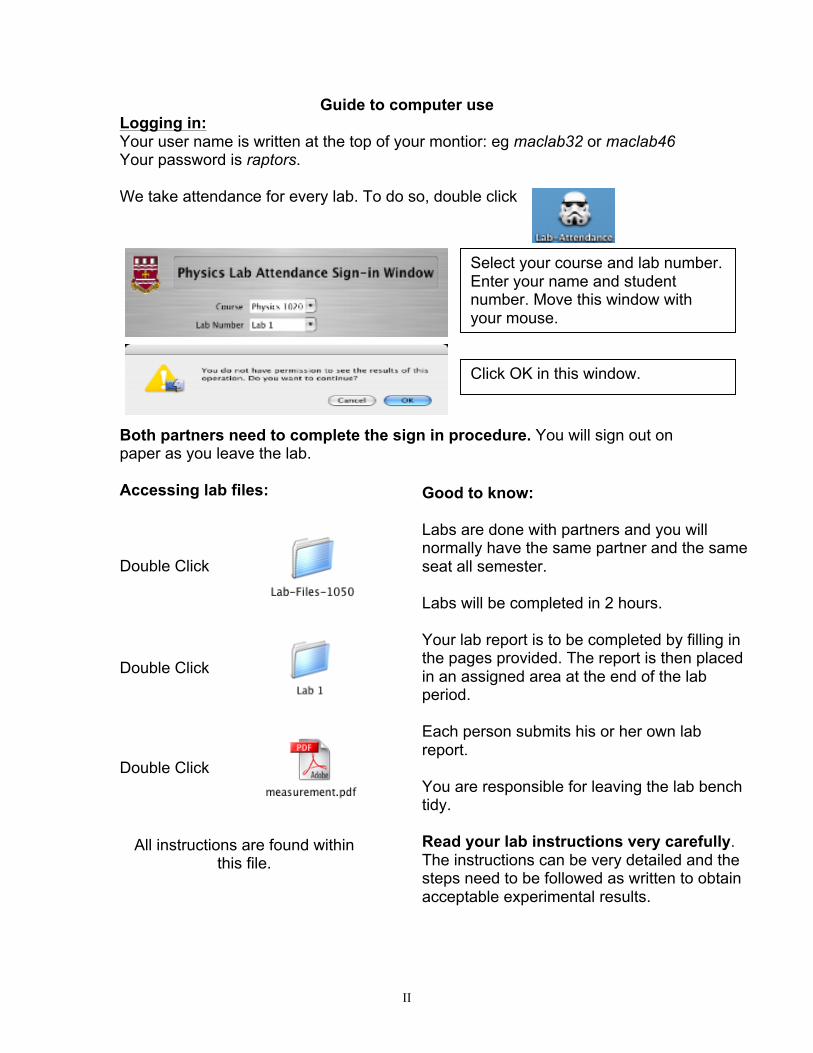
Guide to computer use Logging in: Your user name is written at the top of your montior: eg maclab32 or maclab46 Your password is raptors. We take attendance for every lab. To do so, double click Both partners need to complete the sign in procedure. You will sign out on paper as you leave the lab. Accessing lab files:

Double Click

Double Click

Double Click

All instructions are found within

this file.

Select your course and lab number. Enter your name and student number. Move this window with your mouse.

Click OK in this window.

Good to know: Labs are done with partners and you will normally have the same partner and the same seat all semester. Labs will be completed in 2 hours. Your lab report is to be completed by filling in the pages provided. The report is then placed in an assigned area at the end of the lab period. Each person submits his or her own lab report. You are responsible for leaving the lab bench tidy. Read your lab instructions very carefully. The instructions can be very detailed and the steps need to be followed as written to obtain acceptable experimental results.

III

Memorial University of Newfoundland Department of Physics and Physical Oceanography

Physics 1050 Laboratory

Laboratory Guidelines

1.) All Physics 1050 students are required to complete six experiments. You must obtain a minimum mark of 50% in the laboratory in order to pass the course.

2.) Laboratory classes will be two hours long. Please consult the schedule

posted outside the lab for the exact dates and on the MUN Physics website.

3.) Prelab questions are to be done prior to beginning the laboratory. The

prelab questions are found on the Memorial University physics website at http://www.mun.ca/physics/undergraduates/fylabs/p1050/manual.php.

4.) Laboratory reports will be completed in the lab and are submitted at the

end of the lab period. 5.) Experiments are performed with partners. While partners are expected to

share data and discuss the experiment, each person independently writes his own report. Plagiarism is strictly prohibited.

6.) Keep your work area tidy and return apparatus to the condition in which

you found it. Coats and bags should be placed under the benches or away from areas where people are working. Eating and drinking are not permitted in the laboratory.

7.) If you are absent from the laboratory due to illness, you should contact

your instructor as soon as possible. If you know you will be absent for some other reason, you will need to inform the laboratory instructor beforehand.

8.) Laboratory equipment must be handled with care at all times. All

breakages and accidents must be reported to the instructor immediately. 9.) A first aid kit is available.

IV

Introductory Comments

Computers are important tools in the modern laboratory. Automated data collection allows the experimenter to collect and analyse data in ways that were impractical (or impossible) without computers. The use of computers in the Physics 1050 and Physics 1051 laboratories will introduce you to concepts and techniques you will encounter again in other courses. More importantly, we hope that your experience with computers will give you an appreciation of the ways in which computers and computer-interfaced sensors can be used to study physical phenomena. In many cases, these will substantially simplify and accelerate the process of data collection. Along with the ability to rapidly accumulate large quantities of data comes the growing need for meaningful interpretation of such data. You will be expected to make effective use of your laboratory time for analysis and interpretation of your observations. The experiments in this course have been designed to illustrate important physical principles and to give you experience with electronic data collection and analysis. In order to gain the most benefit from the lab, it is essential that you make an effort to understand both the physical principles underlying the phenomena and the measurement. This manual is divided into two parts: The first part contains a reference section. The second part is your Activity Log. As you perform and analyse each experiment, you will record your observations in these sheets. You will be responsible for understanding the principles of the phenomena you investigate in the laboratory and the methods by which you carry out the investigation.

-V-

Physics 1050 Laboratory

Error Analysis Summary These pages contain some of the basic formulae you will use in order to perform the necessary error analysis in your calculations. Introduction Experimental results always have uncertainty associated with them. It is important to track these uncertainties according to the rules discussed in this manual. Uncertainties arise not from making mistakes in calculations, but from inherent limits in making a measurement. Experimental Error and Uncertainty The difference between a measured or calculated value and the corresponding true value is called the experimental error (or error). Since we usually don’t know the true value of the quantity in question, the values of the experimental errors must be estimated and some judgment is involved in making realistic estimates. An estimate of the experimental error in a quantity is called the uncertainty. Types of Uncertainties Experimental errors arise from a variety of sources and may be broadly classified as random errors and systematic errors. Random errors are those errors that affect the results in a random way, and are equally likely to give values that are too high or too low. As an example, suppose we wish to determine the time for one cycle of a pendulum using a stopwatch. The difficulty of starting and stopping the watch at exactly the correct time (“reaction time error”) means that repeated measurements of this time will differ slightly from each other. This is an example of a random error. Random error can be reduced by taking the average or mean of a set of measurements. Systematic errors are those that tend to affect the experimental results in a consistent way, so all the values are either too high or too low. In the stopwatch example above, if the watch was running slow, all the values would be too low by the same amount, and the effect of this systematic error could not be reduced by taking the average of a set of repeated measurements.

-VI-

Absolute and Relative Uncertainty If δx represents the absolute error or uncertainty in a measured quantity, then

relative uncertainty is given by

€

δxx

The uncertainty is usually rounded to 1 significant figure. A result is generally reported in the form x ± δx. Values with a lower absolute uncertainty have a higher precision. Range The true value of the result is unknown but will lie in the range of x - δx to x + δx. Combining Errors in Laboratory Results Two or more measured quantities are often combined to determine a new quantity. When doing so, the experimental uncertainty of the new quantity must be determined using the following rules. Rule 1: When adding or subtracting measured quantities, the absolute uncertainty in the result is the sum of the absolute uncertainties in the measured quantities. Example 1: z = x – y, δz = δx + δy Example 2: z = x + y, δz = δx + δy Rule 2: When multiplying or dividing measured quantities, the relative uncertainty in the result is the sum of the relative uncertainties in the measured quantities.

Example 1:

€

z =xy

δzz

=δxx

+δyy

-VII-

yy

xx

zzxyz

δδδ+=

=

Rule 3: When multiplying by a constant, the uncertainty is multiplied by the same constant.

xazaxzδδ =

=

Rule 4: Power Laws:

xx

nzzxz n

δδ=

=

Combination of rules: When the desired result depends on more than two quantities, the uncertainty may be calculated by breaking down the algebraic expression term by term. Thus if a = bc2/d, the maximum error in a is given by

€

δaa

=δbb

+ 2δcc

+δdd

Descriptive Statistics: To reduce the effects of random error, we often take N multiple measurements of the same quantity and then take the average or mean

€

x to obtain the best estimate of the “true value”. Mean:

€

x = Σxi

N

Example 2:

-VIII-

We most commonly report standard error

€

σ x as the uncertainty associated with the

average. Standard error is calculated as

€

σ x =σ x

N where

€

σ x is the standard deviation

(a measure of variation about a mean) and is given by

€

σx =(xi∑ − x )2

N −1

-IX-

Sample calculation of standard deviation: In the following tables, calculations are shown for illustrative purposes only. In your Activity Log, you are not required to show workings in your tables. Assume we have taken a set of N = 8 measurements of length and have calculated the mean:

L (m) 21.23 20.98 21.05 20.86 20.78

20.91

20.09 21.62

€

L =ΣLiN

= = 20.94

The next step is to calculate the deviation in each measurement. Deviation is the absolute value of the difference between each measurement and the mean:

L (m)

€

Li − L (m)

21.23 |21.23 – 20.94| = 0.29 20.98 |20.98 – 20.94| = 0.04 21.05 |21.05 – 20.94| = 0.11 20.86 |20.86 – 20.94| = 0.08 20.78 |20.78 – 20.94| = 0.16

20.91 |20.91 – 20.94| = 0.03

20.09 |20.09 – 20.94| = 0.85 21.62 |21.62 – 20.94| = 0.68

€

L =ΣLiN

= 20.94

-X-

We square each deviation and find the sum:

L (m)

€

Li − L

€

Li − L( )2

21.23 |21.23 – 20.94| = 0.29 0.084 20.98 |20.98 – 20.94| = 0.04 0.0016 21.05 |21.05 – 20.94| = 0.11 0.012 20.86 |20.86 – 20.94| = 0.08 0.0064 20.78 |20.78 – 20.94| = 0.16 0.026

20.91 |20.91 – 20.94| = 0.03 0.00090

20.09 |20.09 – 20.94| = 0.85 0.72 21.62 |21.62 – 20.94| = 0.68 0.46

€

L =ΣLiN

= = 20.94

€

Li − L( )2

∑ =1.31

We finish by calculating the standard deviation and then the standard error:

L (m)

€

Li − L (m)

€

Li − L( )2

21.23 |21.23 – 20.94| = 0.29 0.084 20.98 |20.98 – 20.94| = 0.04 0.0016 21.05 |21.05 – 20.94| = 0.11 0.012 20.86 |20.86 – 20.94| = 0.08 0.0064 20.78 |20.78 – 20.94| = 0.16 0.026

20.91 |20.91 – 20.94| = 0.03 0.00090

20.09 |20.09 – 20.94| = 0.85 0.72 21.62 |21.62 – 20.94| = 0.68 0.46

€

L =ΣLiN

= 20.94

€

Li − L( )2

∑ =1.31

€

σ L =Li − L( )

2∑

N −1= 0.433

€

σ L =σ L

N= 0.153

-XI-

We then report our result by rounding the standard error to 1 significant digit and writing it with the mean: L = 20.9 ± 0.2 m. In any given experiment, when reporting a quantity, we choose for the uncertainty either the absolute uncertainty associated with the measuring device or the standard error, whichever is larger. Graphing Summary The Errors in a Straight Line Graph

A straight line graph is described by the equation y=mx+b. The slope (m) and y-intercept (b) can be determined by a statistical treatment known as linear regression. The slope and intercept of a straight line and their errors can easily be determined using mathematical software, such as Graphical Analysis.

-XII-

Use of Software Graphs will normally be drawn with the software package Graphical Analysis. A graph submitted with your lab report should have the format shown at right: • label each axis (double click

axis label in table) • title (double click in white

space) • fit box displayed with

uncertainty (the standard deviation)

• remove connecting lines (double click in white space)

Drawing meaning from your results The slope and intercept of your graph have physical meaning. To determine the meaning of your slope or intercept compare the physical equation to the equation for a straight line. For the graph shown above: Physical Equation: M = ρV (M = mass, ρ = density, V = volume)

Equation for a straight line: y = mx + b

Comparing these equations, we see mass is on the y axis, i.e. y = M, volume is on the x axis, i.e. x = V, and so the slope is the density, i.e. m = ρ. In the above example, we see ρ = 2.706 ± 0.006 g/cm3.

-XIII-

Significant Figures Summary When are digits significant? Non-zero digits are always significant and zeros are significant when between other digits (e.g 4009 has 4 significant digits) or after a decimal point (e.g. 54.03 has 4 significant figures as does 82.00x103). Whole numbers are considered to have infinite significant digits. (e.g. if a hair dryer uses 1.2 kW of power, then 2 identical hairdryers use 2.4 kW (2 significant figures). We typically write in scientific notation to avoid ambiguity with zeros. For example, in 80,400 the significant digits is unknown as the last two zeros may or may not be significant. Instead, we write 8.04x104 indicating there are 3 significant digits. Rules: When multiplying, dividing, performing a trigonometric function, etc. the number of significant digits in the answer will be the same as that of the quantity in the function with the fewest number of significant digits, e.g. 45.5/24 = 1.9 where two significant figures in the answer are kept. When adding or subtracting, the answer will have the same number of digits after the decimal as the quantity in the function with the fewest number of digits after the decimal, e.g. 2.981 + 0.2 = 3.2 where the result keeps one digit after the decimal. Combining answers with uncertainties:

1. Determine the uncertainty first. 2. Round the uncertainty to 1 significant figure. 3. Examine the number. Keep the same number of places after the decimal in the

number as you have in the uncertainty. e.g. An automatic fit to data gives a slope of 2.7061 with an uncertainty of 0.005611. The uncertainty is rounded to 0.006 (1 significant figure). This value has three places after the decimal so the value of 2.7061 is rounded to 2.706 giving a final result of 2.706 +/- 0.006.

Comparing answers and range: When comparing to numbers to see if they agree, write the ranges of both numbers and see if they overlap.

-XIV-

Example: Given two values of acceleration due to gravity: g1 = 9.76± 0.03 m/s2 and g2 = 9.80± 0.02 m/s2 . Do the values agree?

1. Write the range of g1 : 9.73 to 9.79 m/s2 . 2. Write the range of g2 : 9.78 to 9.82 m/s2 . 3. If the ranges overlap, the values agree. If the ranges do not overlap, the values

do not agree. In this case, the ranges do overlap and therefore they agree. Expectation in the lab write up: Data as entered in tables are considered raw data and these entries will not be penalized for mistakes in significant figures rules. Answers given in questions are expected to be written with the correct significant figures obtained by following the rules outlined above.