megan cook, frédéric bouchette, bijan mohammadi, nicolas
TRANSCRIPT

HAL Id: hal-03348827https://hal.archives-ouvertes.fr/hal-03348827
Preprint submitted on 20 Sep 2021
HAL is a multi-disciplinary open accessarchive for the deposit and dissemination of sci-entific research documents, whether they are pub-lished or not. The documents may come fromteaching and research institutions in France orabroad, or from public or private research centers.
L’archive ouverte pluridisciplinaire HAL, estdestinée au dépôt et à la diffusion de documentsscientifiques de niveau recherche, publiés ou non,émanant des établissements d’enseignement et derecherche français ou étrangers, des laboratoirespublics ou privés.
Opti-Morph User GuideMegan Cook, Frédéric Bouchette, Bijan Mohammadi, Nicolas Fraysse
To cite this version:Megan Cook, Frédéric Bouchette, Bijan Mohammadi, Nicolas Fraysse. Opti-Morph User Guide. 2021.�hal-03348827�

Opti-MorphUser Guide
Megan Cook ∗ 1,3,4, Frédéric Bouchette †1,3, Bijan Mohammadi ‡2,3, and Nicolas Fraysse§4
1GEOSCIENCES-M, Univ Montpellier, CNRS, Montpellier, France2IMAG, Univ Montpellier, CNRS, Montpellier, France
3GLADYS, Univ Montpellier, CNRS, Le Grau du Roi, France4BRL Ingénierie, Nîmes, France
September 20, 2021
Abstract
Opti-Morph is a new morphodynamic model based on optimization theory. This user guide explains the theorybehind the model as well as the hydrodynamic models currently associated with Opti-Morph. A presentation of thenumerical model is described to allow the user to run Opti-Morph on their own configurations. Two basic examplesare also provided.
Keywords: optimization, morphodynamics, coastal dynamics, constraints, hydrodynamics
∗Corresponding Author: [email protected]†[email protected]‡bij[email protected]§[email protected]
1

ContentsI Introduction 3
I.1 About . . . . . . . . . . . . . . . . . . . . . . . . . . . . . . . . . . . . . . . . . . . . . . . . . . . 3I.2 Expectations and objectives . . . . . . . . . . . . . . . . . . . . . . . . . . . . . . . . . . . . . . . . 3I.3 Target audience . . . . . . . . . . . . . . . . . . . . . . . . . . . . . . . . . . . . . . . . . . . . . . 3
II Processes and theoretical formulation 4II.1 Domain and definitions . . . . . . . . . . . . . . . . . . . . . . . . . . . . . . . . . . . . . . . . . . 4II.2 Hydrodynamic model . . . . . . . . . . . . . . . . . . . . . . . . . . . . . . . . . . . . . . . . . . . 5
II.2.1 Introduction . . . . . . . . . . . . . . . . . . . . . . . . . . . . . . . . . . . . . . . . . . . . 5II.2.2 Shared processes between hydrodynamic models . . . . . . . . . . . . . . . . . . . . . . . . 6II.2.3 Presentation of hydrodynamic models . . . . . . . . . . . . . . . . . . . . . . . . . . . . . . 8
II.3 Morphodynamic model by wave energy minimization . . . . . . . . . . . . . . . . . . . . . . . . . . 23II.3.1 Introduction . . . . . . . . . . . . . . . . . . . . . . . . . . . . . . . . . . . . . . . . . . . . 23II.3.2 Governing seabed dynamics . . . . . . . . . . . . . . . . . . . . . . . . . . . . . . . . . . . 23II.3.3 Choice of direction of descent . . . . . . . . . . . . . . . . . . . . . . . . . . . . . . . . . . 25II.3.4 Constraints . . . . . . . . . . . . . . . . . . . . . . . . . . . . . . . . . . . . . . . . . . . . 26
III Numerical model 28III.1 Presentation . . . . . . . . . . . . . . . . . . . . . . . . . . . . . . . . . . . . . . . . . . . . . . . . 28
III.1.1 Workflow . . . . . . . . . . . . . . . . . . . . . . . . . . . . . . . . . . . . . . . . . . . . . 28III.1.2 Algorithm summary . . . . . . . . . . . . . . . . . . . . . . . . . . . . . . . . . . . . . . . 31III.1.3 Class organisation . . . . . . . . . . . . . . . . . . . . . . . . . . . . . . . . . . . . . . . . 31
III.2 Running Opti-Morph . . . . . . . . . . . . . . . . . . . . . . . . . . . . . . . . . . . . . . . . . . . 34III.2.1 Getting started . . . . . . . . . . . . . . . . . . . . . . . . . . . . . . . . . . . . . . . . . . 34III.2.2 Main file . . . . . . . . . . . . . . . . . . . . . . . . . . . . . . . . . . . . . . . . . . . . . 35III.2.3 Input data . . . . . . . . . . . . . . . . . . . . . . . . . . . . . . . . . . . . . . . . . . . . . 37III.2.4 Output data . . . . . . . . . . . . . . . . . . . . . . . . . . . . . . . . . . . . . . . . . . . . 39
IV Applications 42IV.1 Linear Seabed Beach Configuration . . . . . . . . . . . . . . . . . . . . . . . . . . . . . . . . . . . 42
IV.1.1 Setting . . . . . . . . . . . . . . . . . . . . . . . . . . . . . . . . . . . . . . . . . . . . . . 42IV.1.2 Input files . . . . . . . . . . . . . . . . . . . . . . . . . . . . . . . . . . . . . . . . . . . . . 42IV.1.3 Results . . . . . . . . . . . . . . . . . . . . . . . . . . . . . . . . . . . . . . . . . . . . . . 43
IV.2 Beach Configuration with submerged breakwaters . . . . . . . . . . . . . . . . . . . . . . . . . . . . 44IV.2.1 Setting . . . . . . . . . . . . . . . . . . . . . . . . . . . . . . . . . . . . . . . . . . . . . . 44IV.2.2 Input files . . . . . . . . . . . . . . . . . . . . . . . . . . . . . . . . . . . . . . . . . . . . . 45IV.2.3 Results . . . . . . . . . . . . . . . . . . . . . . . . . . . . . . . . . . . . . . . . . . . . . . 46
A List of parameters 48
2

I IntroductionI.1 AboutThe numerical hydro-morphodynamic model presented here embodies a new approach to coastal morphodynamics,based on optimization theory. This model is based on the assumption that a sandy seabed evolves over time in order tominimize a certain wave-related function, the choice of which depends on what is considered the driving force behindcoastal morphodynamics. This numerical model was given the name Opti-Morph, and has the advantages of beingfast, robust, and requires very few input parameters.
Optimization theory has been widely used in the study of coastal zones, but is mainly applied in the developmentof protection structures [Isèbe et al., 2008a, Isèbe et al., 2008b] and/or ports [Cook et al., 2021c, Isèbe et al., 2008b].Continuing the pioneering work of [Bouharguane et al., 2010, Mohammadi and Bouharguane, 2011] and[Mohammadi and Bouchette, 2014], which put in motion the idea that morphodynamic processes can be describedusing optimization theory, we have developed a numerical model that simulates the evolution of the seabed while takinginto account the complex coupling between morphodynamic and hydrodynamic processes. Based on the assumptionthat the seabed adapts to minimize a certain hydrodynamic quantity, this optimization problem is also subjected to acertain number of constraints, allowing for a more accurate description of the morphodynamic evolution. First resultscan be found in [Cook et al., 2021b], where this model was applied to a flume configuration and compared with physicaldata. A comparative analysis was also conducted between Opti-Morph and another numerical model for the purposeof evaluating the performance of Opti-Morph in comparison with existing hydro-morphodynamic models.
I.2 Expectations and objectivesThe main goal of Opti-Morph is to demonstrate the potential of using optimal control in the modeling of coastaldynamics by designing an adaptable, easy-to-use numerical model.
A non-exhaustive list of objectives considered during the initial development of Opti-Morph follows.
Ô Production of logical/naturalistic simulation results
Ô Adaptable to open-sea or flume configurations
Ô Low run times
Ô High robustness
Ô User-friendly (including inexperienced users)
Ô Adaptability of:
Þ hydrodynamic model
Þ cost function
Þ constraints
Ô Possibility of introducing submerged breakwaters or other soft engineering techniques
I.3 Target audienceThe Opti-Morph model is a tool intended for any person wishing to simulate the natural evolution of the coastal seabedin response to the incoming wave conditions, and/or to study the effect of man-made submerged devices on the sedimenttransport. As such this tool can be used by engineers and project managers when planning the deployment of certainwave-reducing structures and their influence on the surrounding sediment.
This model can also be used in an academic setting to study the driving forces behind coastal morphodynamics. Themodel has been developed such that the mobility of the seabed is driven by the minimization of a cost function. The
3

choice of cost function determines which coastal hydro-morphodynamic components drive the seabed mobility. Thedefault cost function is wave energy but other functions can be explored if desired.
II Processes and theoretical formulationThe Opti-Morph model operates by pairing a hydrodynamic and a morphodynamic model. The basis of the morpho-dynamic model is the minimization of a wave-related cost function; this cost function is provided by the hydrodynamicmodel, which demonstrates the close relation between the hydrodynamic and morphodynamic processes. In this firstsection, we will begin by describing the domain and definitions used throughout this document. The hydrodynamicmodel is then described with its various adaptations, followed by the theoretical description of the morphodynamicmodel. This includes the governing equations, the choice of cost function, and the introduction of the notion ofconstraints.
II.1 Domain and definitionsWe consider a coordinate system composed of a horizontal axis G and a vertical axis I. We denote Ω := [0, Gmax] thedomain of the cross-shore profile, where G = 0 refers to an arbitrary fixed point in the deep water and Gmax an arbitraryfixed point at the shore, beyond the coast. The elevation of the seabed is a one-dimensional positive function, definedby: k : Ω × [0, )] ×Ψ→ R+ where [0, )] is the interval of time considered for the study, and Ψ is the set of physicalparameters describing the shape of the seabed. Let ℎ0 be the mean water level (<) and ℎ be the water depth (<), definedover the cross-shore profile by ℎ = ℎ0 − k. We denote ΩS the sub-domain of Ω over which the waves shoal and ΩB thesub-domain of Ω over which the waves break. Let GB denote the location of the breaking of the waves and let GS bethe shoreline position, that is when the seabed intersects with the mean water level ℎ0. Note that the breaking locationand the shoreline position may vary over the course of the simulation, and as such GB and GS are both time-dependent.The same also goes for ΩB and ΩS. Time dependency of GB, GS, ΩB and ΩS have been omitted for clarity from theremainder of this document. The definitions and notations presented above are summarized in Figure 1.
Figure 1: Illustration of the cross-shore profile where breaking occurs once at G = GB
� At the present time, Opti-Morph operates in a one-dimensional setting, depicting either the cross-shore profile ofa sandy beach or a flume experiment. However, no assumptions were made regarding the choice of dimension in thetheoretical development of this model, and as a result, it is straightforward to extend this theory to a two-dimensionalconfiguration.
4

II.2 Hydrodynamic modelII.2.1 Introduction
In order to model the evolution over time of the seabed k and given the assumption that k changes over time in responseto the minimization of some hydrodynamic quantity, a hydrodynamic model capable of providing the necessary datais required, here the significant wave height over the cross-shore profile.
There are currently seven different hydrodynamic models associated with the Opti-Morph model. These hydrodynamicmodels have the advantage of being able to analytically calculate the gradient of wave height with respect to theseabed. Indeed, Opti-Morph relies heavily on this differentiation, and explicit formulas induce quick execution times.Considering that one of the main objectives of Opti-Morph is a rapid output time (cf. Section I.2), it is natural for theassociated hydrodynamic models to also have significantly fast execution times. This is achieved by providing waveheight analytically with regard to the seabed k. Other hydrodynamic models can be integrated with ease, provided thatthe parameters and methods required by the morphodynamic model are still present. A model using a time-consumingdifferentiation method can be used but defeats the purpose of Opti-Morph which was designed to be quick and oflow-complexity. Another solution would be to perform the calculation of the gradient using automatic differentiationprograms [Griewank and Walther, 2008, Hascoët and Pascual, 2004]. This exceeds the initial scope of the Opti-Morphmodel, but may be implemented at some point in the future if needs be.
The seven hydrodynamic models presented below provide the significant wave height over the cross-shore profile aswell as other wave-related data. They range in complexity, from the simplest model in II.2.3.a. to the more complexin II.2.3.g.. In fact, the hydrodynamic models, and the order in which they appear, illustrate the evolution of themodel over the course of its development, with the last being the final product. This was carried out in an attempt toaddress the different issues encountered during the research phase. Each model has its own merits and all have beenretained in order to demonstrate the simplicity of replacing one hydrodynamic model with another. This evolution ofthe hydrodynamic model is showcased in Table 1.
5
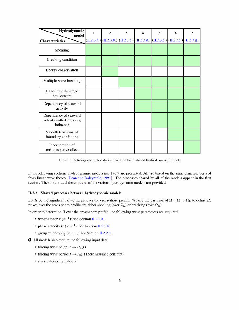
Characteristics
Hydrodynamicmodel 1 2 3 4 5 6 7
(II.2.3.a.) (II.2.3.b.) (II.2.3.c.) (II.2.3.d.) (II.2.3.e.) (II.2.3.f.) (II.2.3.g.)
Shoaling
Breaking condition
Energy conservation
Multiple wave-breaking
Handling submergedbreakwaters
Dependency of seawardactivity
Dependency of seawardactivity with decreasing
influence
Smooth transition ofboundary conditions
Incorporation ofanti-dissipative effect
Table 1: Defining characteristics of each of the featured hydrodynamic models
In the following sections, hydrodynamic models no. 1 to 7 are presented. All are based on the same principle derivedfrom linear wave theory [Dean and Dalrymple, 1991]. The processes shared by all of the models appear in the firstsection. Then, individual descriptions of the various hydrodynamic models are provided.
II.2.2 Shared processes between hydrodynamic models
Let � be the significant wave height over the cross-shore profile. We use the partition of Ω = ΩS ∪ ΩB to define �:waves over the cross-shore profile are either shoaling (over ΩS) or breaking (over ΩB).
In order to determine � over the cross-shore profile, the following wave parameters are required:
• wavenumber : (<−1): see Section II.2.2.a.
• phase velocity � (<.B−1): see Section II.2.2.b.
• group velocity �g (<.B−1): see Section II.2.2.c.
� All models also require the following input data:
• forcing wave height C → �0 (C)
• forcing wave period C → )0 (C) (here assumed constant)
• a wave-breaking index W
6

II.2.2.a. Wavenumber
The wavenumber is determined by the linear dispersion equation. Linear dispersion is given by:
f2 = 6: tanh(:ℎ) (1)
where f = 2c)0
is the wave pulsation (B−1), 6 ≈ 9.81 <.B−2 is the gravitational acceleration, and : is the wavenumber(<−1). Recalling that : = 2c
!, this equation states that waves with different wavelengths ! (<) travel at different speeds
� (<.B−1). Here, we use it to determine the wavenumber : by using a recursive algorithm such as the Newton-Raphsonmethod.
II.2.2.b. Phase velocity
The phase velocity of a wave � (<.B−1) is given by:
� (G, C) = �0 (C) tanh(: (G, C)ℎ(G, C)) ∀(G, C) ∈ Ω × [0, )] (2)
where �0 is the velocity of the forcing waves (<.B−1), defined here by �0 (C) = 6
2c)0 (C) for all C ∈ [0, )].
II.2.2.c. Group velocity
The group velocity of a wave �g (<.B−1) is given by:
�g =12�
(1 + 2:ℎsinh 2:ℎ
)∀(G, C) ∈ Ω × [0, )] (3)
Let = be is the ratio of the wave velocity with respect to the group velocity: = = �g�.
II.2.2.d. Wave height
For all G ∈ ΩS and C ∈ [0, )], we define the shoaling wave height �S as:
�S (G, C) = �0 (C) S (G, C) (4)
where �0 is the height of the forcing waves and S is the shoaling coefficient (-) defined by Equation (5).
S (G, C) =(1
2=(G, C)�0 (C)� (G, C)
)1/2∀(G, C) ∈ ΩS × [0, )] (5)
II.2.2.e. Breaking wave height
The equations governing breaking wave height (over ΩB) vary according to the choice of hydrodynamic model.However, all use the breaking condition first established by [Munk, 1949], which states that waves break when theirheight is too great with respect to the water depth. In other words, waves break when inequality (6) holds, where W isa wave-breaking index. This parameter is set to 0.55 in the upcoming simulations (cf. Section IV).
�
ℎ> W (6)
Using this wave-breaking condition, we can define ΩS and ΩB as:
ΩS (C) ={G ∈ Ω, � (G, C)
ℎ(G, C) < W}
and ΩB =
{G ∈ Ω, � (G, C)
ℎ(G, C) ≥ W}
(7)
� The domain over which � is defined as the disjoint union of ΩS and ΩB: [0, GS] = ΩS ∪ΩB and ΩS ∪ΩB = ∅.
7

II.2.3 Presentation of hydrodynamic models
II.2.3.a. Hydrodynamic model no.1: Shoaling model with decreasing exponential breaking
Technical features
Technical features
• Code name: shoaling_1run
• Use: Regular seabed
• Advantages: Very fast; Known wave-breaking type
• Inconveniences: One wave-breaking allowed; wave-breaking type must be known
• Additional entry parameters: U: wave-breaking parameter
• Description: Shoaling until breaking then decreasing exponentially with thealpha parameters describing the descent.
• Governing equations:
� (G, C) =
�0 (C) S (G, C) for G ∈ [0, GB]
�S (GB)4−U(G−GB) − 4−U(GS−GB)
1 − 4−U(GS−GB)for G ∈ [GB, GS]
for all (G, C) ∈ Ω × [0, )], where U is user-defined.
o Time dependency of GB and GS have been omitted for clarity.
Detailed descriptionWe assume that waves shoal the length of the cross-shore profile until the breaking condition (6) is first activated.This point is denoted GB. From then on, waves break up until the shoreline GS, decreasing in height until � (GB) = 0.Breaking wave height is described as a simple decreasing exponential function from GB to GS: for all G ∈ ΩB = [GB, GS],wave height is given by:
� (G, C) = �S (GB)4−U(G−GB) − 4−U(GS−GB)
1 − 4−U(GS−GB)(8)
where the parameter U determines the manner in which the waves break (cf. Figure 2).
Figure 2: Different values of U alter the behavior of the breaking waves.
� This function was designed such that the resulting wave height over the cross-shore profileΩ is a continuous functionwith zero wave height at the shoreline i.e.� (GB) = �S (GB) and � (GS) = 0.
Combined with the shoaling equation (4) over ΩS = [0, GB], Hydrodynamic model no.1 provides wave height over thecross-shore profile using the following definition:
8

� (G, C) =
�S (G, C) for G ∈ [0, GB]
�S (GB)4−U(G−GB) − 4−U(GS−GB)
1 − 4−U(GS−GB)for G ∈ [GB, GS]
(9)
for all G ∈ Ω and C ∈ [0, )].
Note that breaking may occur only once, and therefore ΩB and ΩS are both connected sets.
IllustrationAn illustration of the the wave height provided by this model is given in Figure 3 on different types of seabeds.
(a) Wave height calculated over a linearseabed
(b) Wave height calculated over a linearseabed with submerged breakwater
(c) Wave height calculated over an experi-mental seabed (with natural sandbar)
Figure 3: Illustration of Hydrodynamic model no.1 on different seabeds
All three examples of wave height look alike: waves shoal in the deeper waters then decrease exponentially to reachzero at the shore.
� This model is recommended on all seabeds, on the condition that the user is content with having waves only breakingonce along the cross-shore profile. It is also the faster of the models.
II.2.3.b. Hydrodynamic model no.2: Shoaling model with decreasing exponential breaking and energy con-servation
Technical features
9

Technical features
• Code name: shoaling_2run
• Use: Regular seabed
• Advantages: Very fast; Guarantees conservation of wave energy between sedimentdisplacement (for a same forcing condition)
• Inconveniences: One wave-breaking allowed
• Additional entry parameters: UC=0: initial breaking decrease parameter
• Description: Shoaling until breaking then decreasing exponentially with U(C)chosen for energy conservation.
• Governing equations:
� (G, C) =
�0 (C) S (G, C) for G ∈ [0, GB]
�S (GB)4−U(C) (G−GB) − 4−U(C) (GS−GB)
1 − 4−U(C) (GS−GB)for G ∈ [GB, GS]
for all (G, C) ∈ Ω × [0, )], where U is determined to ensure conservation of waveenergy between sediment displacement.
o Time dependency of GB and GS have been omitted for clarity.
Detailed descriptionThis model is based on the principle of energy conservation. Given two wave height functions �1 and �2 originatingfrom the same forcing �0, we should have conservation of energy, irrespective of the shape of the seabed. Therefore,the energy of the system should be the same before and after applying the morphodynamic model.
To achieve this, we implement the following workflow:
• Step 1: Apply Hydrodynamic model with user defined parameters
• Step 2: Apply Morphodynamic model
• Step 3: Apply Hydrodynamic model with parameters selected to ensure energy conservation
We adopt the previous hydrodynamic model from Section II.2.3.a., but allow variations of the value of the parameterU to guarantee energy conservation. This implies that waves break differently depending on the forcing wave energy.
Step 1: In Step 1, the wave height over the cross-shore profile is set as:
� (G, C) =
�S (G) for G ∈ [0, GB]
�S (GB)4−U(G−GB) − 4−U(GS−GB)
1 − 4−U(GS−GB)for G ∈ [GB, GS]
(10)
for all G ∈ Ω and C ∈ [0, )]. Here, �S is once again given by the shoaling equation (4) and U is user-defined as aprediction of the type of breaking waves.
Step 2: The morphodynamic model is then applied which provides the new seabed elevation function k in responseto the forcing conditions at time C.
10

Step 3: Here, we consider that waves break as per Equation (10), but U is no longer user-defined. We now need todetermine the breaking parameter U such that energy is conserved.
Let �1, E1, G(1 , G�1 ,Ω(1 and Ω(1 (resp. �2, E2, G(2 , G�2 , Ω(2 and Ω(2 ) be the wave height, wave energy, shoreline andbreaking point, shoaling zone and breaking zone before (resp. after) the morphodynamic changes.
Conservation of energy implies:
E1 = E2 ⇒116
∫Ω
dw6�21 =
116
∫Ω
dw6�22 (11)
⇒∫Ω
�21︸︷︷︸�
=
∫Ω(2
�223G︸ ︷︷ ︸�
+�2 (G�2 )2∫Ω�2
(4−U(G−G�2 ) − 4−U(G(2−G�2 )
1 − 4−U(G(2−G�2 )
)23G (12)
⇒ � − ��2 (G�2 )
=
∫Ω�2
(4−U(G−G�2 ) − 4−U(G(2−G�2 )
1 − 4−U(G(2−G�2 )
)23G (13)
o Wave height over Ω \ (ΩS ∪ΩB) is zero.
The quantities � and � are easily calculated. Using a Newton-Raphson method, we can determine U such that Equation(13) holds, and therefore energy is conserved between morphodynamic changes.
To conclude, the Hydrodynamic Model no.2 provides wave height over the cross-shore profile using the followingdefinition: For all (G, C) ∈ Ω × [0, )]
� (G, C) =
�S (G) for G ∈ [0, GB]
�S (GB)4−U(C) (G−GB) − 4−U(C) (GS−GB)
1 − 4−U(C) (GS−GB)for G ∈ [GB, GS]
(14)
where U(C) is the time-dependent breaking parameter ensuring conservation of energy at time C ∈ [0, )].
IllustrationAn illustration of the the wave height provided by this model is given in Figure 4 on different types of seabeds.
(a) Wave height calculated over a linearseabed
(b) Wave height calculated over a linearseabed with submerged breakwater
(c) Wave height calculated over an experi-mental seabed (with natural sandbar)
Figure 4: Illustration of Hydrodynamic model no.2 on different seabeds
Similar to before, all three examples of wave height look alike: waves shoal in the deeper waters then decreaseexponentially to reach zero at the shore. The only difference is the value of U which differs over time.
11
� This model is recommended on all seabeds, on the condition that the user is content with waves only breaking onceacross the cross-shore profile.
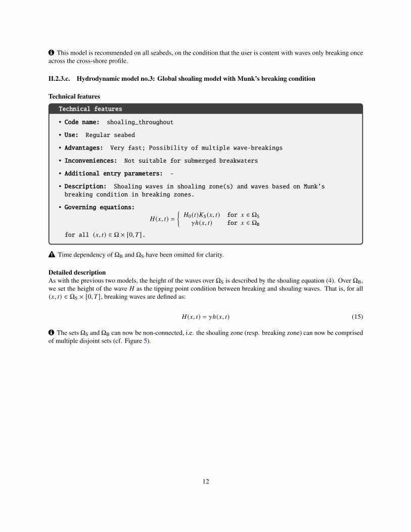
II.2.3.c. Hydrodynamic model no.3: Global shoaling model with Munk’s breaking condition
Technical features
Technical features
• Code name: shoaling_throughout
• Use: Regular seabed
• Advantages: Very fast; Possibility of multiple wave-breakings
• Inconveniences: Not suitable for submerged breakwaters
• Additional entry parameters: -
• Description: Shoaling waves in shoaling zone(s) and waves based on Munk’sbreaking condition in breaking zones.
• Governing equations:
� (G, C) ={�0 (C) S (G, C) for G ∈ ΩSWℎ(G, C) for G ∈ ΩB
for all (G, C) ∈ Ω × [0, )].
o Time dependency of ΩB and ΩS have been omitted for clarity.
Detailed descriptionAs with the previous two models, the height of the waves over ΩS is described by the shoaling equation (4). Over ΩB,we set the height of the wave � as the tipping point condition between breaking and shoaling waves. That is, for all(G, C) ∈ ΩS × [0, )], breaking waves are defined as:
� (G, C) = Wℎ(G, C) (15)
� The sets ΩS and ΩB can now be non-connected, i.e. the shoaling zone (resp. breaking zone) can now be comprisedof multiple disjoint sets (cf. Figure 5).
12

Figure 5: Multiple wave-breakings are now possible, which leads to ΩS and ΩB being potentially disconnected
Therefore, Hydrodynamic model no.3 provides wave height over the cross-shore profile using the following definition:
� (G, C) ={�0 (C) S (G, C) for G ∈ ΩSWℎ(G, C) for G ∈ ΩB
(16)
IllustrationAn illustration of the the wave height provided by this model is given in Figure 6 on different types of seabeds.
(a) Wave height calculated over a linearseabed
(b) Wave height calculated over a linearseabed with submerged breakwater
(c) Wave height calculated over an experi-mental seabed (with natural sandbar)
Figure 6: Illustration of Hydrodynamic model no.3 on different seabeds
When waves break, wave height closely follows the profile of the seabed, since over ΩB, � = W(ℎ0 − k), by definitionof ℎ. As such, for a linear seabed, the breaking descent is linear (Fig. 6a). For the configuration with submergedbreakwater, the shape of the structure is outlined (Fig. 6b). The structure triggers breaking but wave height quicklyresumes it’s previous state. This demonstrates that this model is not equipped to manage underwater structures or anyirregular seabed. This is also shown in Figure 6c, where the natural sandbar starts the breaking phenomenon, but waveheight increases unrealistically once the sandbar has been passed. This model does however have the advantage ofallowing multiple breakings. Breaking occurs twice in Figures 6b and 6c, once at the breakwater/sandbar and oncefurther toward the coast.
� This model is recommended on regular seabeds, but is unable to handle irregular seabed such as those withsubmerged breakwaters or natural sandbars.
13

II.2.3.d. Hydrodynamic model no.4: Local shoaling model with Munk’s breaking condition
Technical features
Technical features
• Code name: shoaling_incremental
• Use: Regular or irregular seabeds
• Advantages: Very fast; Possibility of multiple wave-breakings
• Inconveniences: Unstable (due to the iterative nature of the model)
• Additional entry parameters: -
• Description: Local shoaling waves in shoaling zone(s) and waves based on Munk’sbreaking condition in breaking zones.
• Governing equations:
� (G, C) ={� (G − Y) S (G, C) if G ∈ ΩS
Wℎ(G, C) if G ∈ ΩB
for all (G, C) ∈ Ω × [0, )].
o Time dependency of ΩB and ΩS have been omitted for clarity.
Detailed descriptionInstead of considering that a wave is spatially dependent on only the initial wave height, this model considers thatwave height depends on the seaward activity of the waves. In a configuration with a local sandbar or wave-breakingstructure, waves determined by the previous model (Section II.2.3.c.) shoal up until the structure and then break whenthe structure is detected. However, once the waves move beyond the wave-breaking device, they resume a wave heightsimilar to that before the structure, i.e. disregarding the encounter of the wave-breaking structure. In other words, themodel doesn’t register the loss of energy that took place at the submerged wave-breaker. This is due to the fact thatthe only spacial component influencing the wave height across the cross-shore profile is at G = 0 (by way of the term�0 (C)). This model amends this.
Instead of using wave height at the entry of the domain at each point G of the cross-shore profile Ω, we now use theprevious seaward point of the domain discretization, located at G−Y. Therefore, shoaling waves, which were previouslydescribed by (4) is now defined by:
� (G, C) = � (G − Y) S (G, C) (17)
for all G ∈ ΩS and C ∈ [0, )], where G − Y is the previous point of the discretization.
With the same breaking process as before over ΩB, i.e. Equation (15), wave height is now described by the followingequation:
� (G, C) ={� (G − Y) S (G, C) for G ∈ ΩS
Wℎ(G, C) for G ∈ ΩB(18)
for all (G, C) ∈ Ω × [0, )].
14

o Taking the previous point of the discretization guarantees that submerged breakwaters are taken into account.However, the iterative nature of the model leads to unstable results. Increasing Y would render the model more stable,but results in a poor management of the submerged breakwaters once again.
IllustrationAn illustration of the the wave height provided by this model is given in Figure 7 on different types of seabeds.
(a) Wave height calculated over a linearseabed
(b) Wave height calculated over a linearseabed with submerged breakwater
(c) Wave height calculated over an experi-mental seabed (with natural sandbar)
Figure 7: Illustration of Hydrodynamic model no.4 on different seabeds
Figure 7 shows that this model can handle the introduction of geotubes. The structure causes the waves to breakprematurely. Wave height drops and shoaling resumes. This is also true for natural sandbars. Once the waves break,waves can once again shoal, allowing for multiple breakings if necessary.
� This model is not recommended for Opti-Morph because of the unstable effect it has on the seabed.
II.2.3.e. Hydrodynamic model no.5: Weighted window local shoaling model
Technical features
15

Technical features
• Code name: shoaling_window
• Use: Regular or irregular seabeds
• Advantages: Fast; Possibility of multiple wave-breakings; Takes into account theeffect of the seawards waves; Handles submerged breakwaters
• Inconveniences: Poor management of deep sea conditions
• Additional entry parameters: 3w: maximal distance of local spatial dependency ofa wave
• Description: Seaward waves influence wave height with decreasing effect
• Governing equations:
� (G, C) =�F0 (G, C) S (G, C) for G ∈ ΩS
Wℎ(G, C) for G ∈ ΩB
for all (G, C) ∈ Ω × [0, )], where �F0 is the weighted average of the seaward waves.
o Time dependency of ΩB and ΩS have been omitted for clarity.
Detailed descriptionInstead of considering that waves depend solely on offshore wave height �0 as in II.2.3.c., or a nearby seaward pointas in II.2.3.d., this model suggests that shoaling waves are decreasingly influenced by seawards waves. The greaterthe distance, the less effect it has of the present wave height. Let 3w > 0 be the maximal distance of local spatialdependency of a wave. Wave height at G ∈ ΩS depends on the behavior of the wave height over the interval [G − 3w, G)with a strong influence at the upper-bound and little to no influence at the lower-bound. As such, we introduce aweighting function F, defined over [0, 3w] and quantifies the influence of the seawards waves on the current wave. Itis defined such that F(0) = 1 , F(3w) = 0 and decreases exponentially:
F : [0, 3w] −→ R+
G ↦−→ exp
(ln(0.01)
(G
3win
)2) (19)
16

Figure 8: Weighting function F, equal to 1 closest to the present wave and decreases exponentially as the distanceseaward increases
An illustration of the weighting function F is given in Figure 8. However, if breaking occurs, the history of the waveprior to breaking should not be relevant. This is to ensure that once the energy of the waves is lost due to breaking, itcannot be regained. The term �0 in equation (4) (or the term � (· − Y) in (17)) is now replaced by a weighted averageof the seaward wave height, denoted �F0 and defined as:
�F0 (G, C) =1∫ G
G−- F(G − H)dH
∫ G
G−-F(G − H)� (H) (H)dH (20)
where - = min(G, 3w, dist(G, GB)). Introducing - ensures wave history is taking into account over the appropriate zone:- = G indicates that the zone of local spatial dependency is cut off by the lower-bound of the domain, - = 3w depictswave dependency over the maximal distance, and - = dist(G, GB) indicates that the zone of local spatial dependency isinterrupted by waves breaking.
Shoaling waves are therefore described by:
� (G, C) = �F0 (G, C) S (G, C) (21)
for all G ∈ ΩS and C ∈ [0, )].
As such, wave height over the cross-shore profile Ω is given by:
� (G, C) =�F0 (G, C) S (G, C) for G ∈ ΩS
Wℎ(G, C) for G ∈ ΩB
(22)
IllustrationAn illustration of the the wave height provided by this model is given in Figure 9 on different types of seabeds.
17
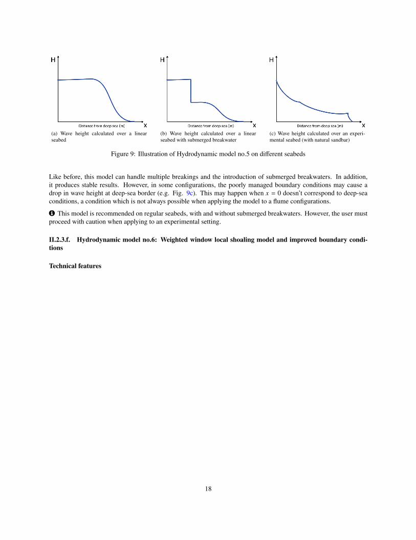
(a) Wave height calculated over a linearseabed
(b) Wave height calculated over a linearseabed with submerged breakwater
(c) Wave height calculated over an experi-mental seabed (with natural sandbar)
Figure 9: Illustration of Hydrodynamic model no.5 on different seabeds
Like before, this model can handle multiple breakings and the introduction of submerged breakwaters. In addition,it produces stable results. However, in some configurations, the poorly managed boundary conditions may cause adrop in wave height at deep-sea border (e.g. Fig. 9c). This may happen when G = 0 doesn’t correspond to deep-seaconditions, a condition which is not always possible when applying the model to a flume configurations.
� This model is recommended on regular seabeds, with and without submerged breakwaters. However, the user mustproceed with caution when applying to an experimental setting.
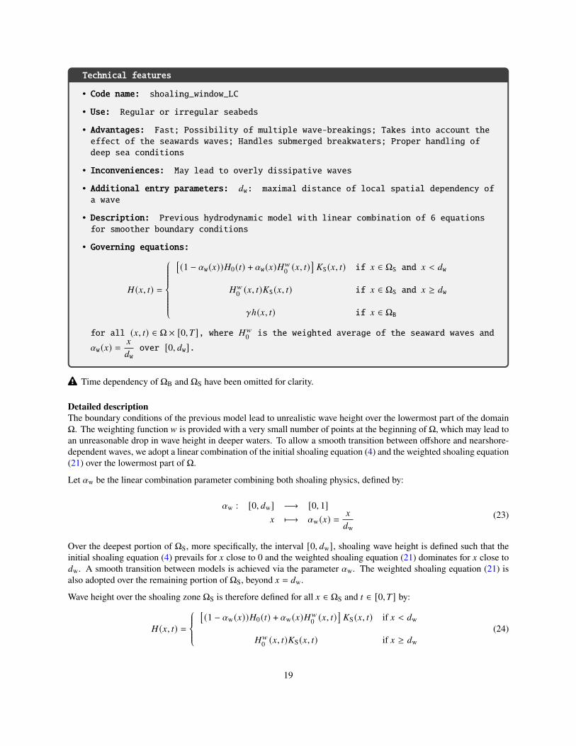
II.2.3.f. Hydrodynamic model no.6: Weighted window local shoaling model and improved boundary condi-tions
Technical features
18
Technical features
• Code name: shoaling_window_LC
• Use: Regular or irregular seabeds
• Advantages: Fast; Possibility of multiple wave-breakings; Takes into account theeffect of the seawards waves; Handles submerged breakwaters; Proper handling ofdeep sea conditions
• Inconveniences: May lead to overly dissipative waves
• Additional entry parameters: 3w: maximal distance of local spatial dependency ofa wave
• Description: Previous hydrodynamic model with linear combination of 6 equationsfor smoother boundary conditions
• Governing equations:
� (G, C) =
[(1 − Uw (G))�0 (C) + Uw (G)�F0 (G, C)
] S (G, C) if G ∈ ΩS and G < 3w
�F0 (G, C) S (G, C) if G ∈ ΩS and G ≥ 3w
Wℎ(G, C) if G ∈ ΩB
for all (G, C) ∈ Ω × [0, )], where �F0 is the weighted average of the seaward waves andUw (G) =
G
3wover [0, 3w].
o Time dependency of ΩB and ΩS have been omitted for clarity.
Detailed descriptionThe boundary conditions of the previous model lead to unrealistic wave height over the lowermost part of the domainΩ. The weighting function F is provided with a very small number of points at the beginning of Ω, which may lead toan unreasonable drop in wave height in deeper waters. To allow a smooth transition between offshore and nearshore-dependent waves, we adopt a linear combination of the initial shoaling equation (4) and the weighted shoaling equation(21) over the lowermost part of Ω.
Let Uw be the linear combination parameter combining both shoaling physics, defined by:
Uw : [0, 3w] −→ [0, 1]G ↦−→ Uw (G) =
G
3w
(23)
Over the deepest portion of ΩS, more specifically, the interval [0, 3w], shoaling wave height is defined such that theinitial shoaling equation (4) prevails for G close to 0 and the weighted shoaling equation (21) dominates for G close to3w. A smooth transition between models is achieved via the parameter Uw. The weighted shoaling equation (21) isalso adopted over the remaining portion of ΩS, beyond G = 3w.
Wave height over the shoaling zone ΩS is therefore defined for all G ∈ ΩS and C ∈ [0, )] by:
� (G, C) =
[(1 − Uw (G))�0 (C) + Uw (G)�F0 (G, C)
] S (G, C) if G < 3w
�F0 (G, C) S (G, C) if G ≥ 3w(24)
19

Adopting the same wave height equation over ΩB as before, with Equation (15), wave height over the cross-shoredomain is defined for all (G, C) ∈ Ω × [0, )] by:
� (G, C) =
[(1 − Uw (G))�0 (C) + Uw (G)�F0 (G, C)
] S (G, C) for G ∈ ΩS and G < 3w
�F0 (G, C) S (G, C) for G ∈ ΩS and G ≥ 3w
Wℎ(G, C) for G ∈ ΩB
(25)
IllustrationAn illustration of the the wave height provided by this model is given in Figure 10 on different types of seabeds.
(a) Wave height calculated over a linearseabed
(b) Wave height calculated over a linearseabed with submerged breakwater
(c) Wave height calculated over an experi-mental seabed (with natural sandbar)
Figure 10: Illustration of Hydrodynamic model no.6 on different seabeds
Now that the boundary condition has been properly dealt with, we no longer observe the unusual drop at the beginningof the domain. Acceptable wave height is produced in all three settings.
� This model is recommended on regular seabeds, with and without submerged breakwaters, as well as in experimentalsettings.
II.2.3.g. Hydrodynamic model no.7: Weighted window shoaling model with anti-dissipative effect
Technical features
20

Technical features
• Code name: shoaling_window_LC_ADT
• Use: Regular or irregular seabeds
• Advantages: Fast; Possibility of multiple wave-breakings; Takes into account theeffect of the seawards waves; Handles submerged breakwaters; Proper handling ofdeep sea conditions; Control of the dissipative effect of the waves;
• Inconveniences: TBA
• Additional entry parameters: 3w: maximal distance of local spatial dependency ofa wave; 0AD and 1AD: anti-dissipative parameters
• Description: Previous hydrodynamic model with the possibility of including ananti-dissipative term.
• Governing equations:
� (G, C) = jAD (G)
[(1 − Uw (G))�0 (C) + Uw (G)�F0 (G, C)
] S (G, C) for G ∈ ΩS and G < 3w
�F0 (G, C) S (G, C) for G ∈ ΩS and G ≥ 3w
Wℎ(G, C) for G ∈ ΩB
for all (G, C) ∈ Ω × [0, )], where �F0 is the weighted average of the seaward waves,Uw (G) = G
3wover [0, 3w] and jAD is an anti-dissipative term.
o Time dependency of ΩB and ΩS have been omitted for clarity.
Detailed descriptionDepending on the required wave behavior, it may be necessary to limit the dissipation of the waves. Indeed, one maydiscover that the hydrodynamic model of section II.2.3.f. dissipates too much energy over the cross-shore profile. Thisis especially relevant when comparing the numerical wave height with experimental data. For the purposes of allowingthe user to calibrate the dissipation of the shoaling waves, we introduce the following anti-dissipative term jAD:
jAD (G) =
(1 + 0AD
G
Gmax
)1AD−
(1 + 0AD
GΩ−S (G)Gmax
)1AD+ 1 for G ∈ ΩS
1 for G ∈ ΩB
(26)
where GΩ−S (G) is the lower-bound of the connected subset of ΩS where G is found. The parameters 0AD and 1AD allowthe user to define the manner in which the waves dissipate; 0AD determines the slope of jAD and 1AD its quadraticbehavior. An example of the anti-dissipative term is given in Figure 11, with 1AD > 1.
21

Figure 11: Example of the anti-dissipative term
� Setting (0AD, 1AD) = (0, 1) disables the anti-dissipative effect.
Wave height over the cross-shore profile Ω is defined by:
� (G, C) = jAD (G)
[(1 − Uw (G))�0 (C) + Uw (G)�F0 (G, C)
] S (G, C) for G ∈ ΩS and G < 3w
�F0 (G, C) S (G, C) for G ∈ ΩS and G ≥ 3w
Wℎ(G, C) for G ∈ ΩB
(27)
for all (G, C) ∈ Ω × [0, )].
This is the model used in the subsequent applications of Section IV.
IllustrationAn illustration of the the wave height provided by this model is given in Figure 12 on different types of seabeds.
(a) Wave height calculated over a linearseabed
(b) Wave height calculated over a linearseabed with submerged breakwater
(c) Wave height calculated over an experi-mental seabed (with natural sandbar)
Figure 12: Illustration of Hydrodynamic model no.7 on different seabeds
With the proper choice of 0AD and 1AD, we can now calibrate the hydrodynamic model to fit the required profile. Thisis especially useful in the case of an experimental flume setting where wave height has been collected as part of theexperiment.
� This model is recommended on regular seabeds, with and without submerged breakwaters, as well as in experimentalsettings.
22

II.3 Morphodynamic model by wave energy minimizationII.3.1 Introduction
This section is devoted to the presentation of the Opti-Morph model. This one-of-a-kind morphodynamic modelis based on optimization theory. The fundamental assumption governing Opti-Morph states that the seabed evolvesover time so as to minimize a certain quantity, named cost function. The choice of cost function depends on whatis considered the driving force behind the morphodynamic response to the seabed. Several cost functions have beenconsidered, but all revolve around wave energy. In other words, the shape of the seabed varies in an effort to minimizethe energy of the surface waves at that given time. At each time, the model indicates the direction to a local minimumof the cost function with regard to the parameterization of the seabed. Two physical parameters limit or encourageseabed mobility depending on the proprieties of the sediment and the depth of the water. Furthermore, constraints areadded to this optimization problem as a means to incorporate additional physics to the model. Constraints are regardedas secondary processes in regards to the minimization of the cost function, which is deemed the primary force behindthe morphodynamic response to the seabed. Three constraints have been included in this model. The first concernsthe maximal slope of the seabed, the second manages the sandstock of the profile in the case of an experimental flume,and the third concerns the presence of bedrock.
The optimization problem that Opti-Morph seeks to solve is:
For each C ∈ [0, )], find the shape of the seabed k(C) ∈ Ψ such that the cost function J (C) is minimal, while subjectedto constraints.
This morphodynamic model is associated with one of the hydrodynamic models from section II.2, which provides themorphodynamic model with the necessary hydrodynamic quantities.
II.3.2 Governing seabed dynamics
In order to describe the evolution of the seabed, we assume that at each time C ∈ [0, )], the seabed k, in its effort tominimize a certain energy related quantity J , verifies the following dynamics over Ω:{
kC (·, C) = ΥΛ3 (·, C)k(·, 0) = k0 (·)
(28)
where kC is the evolution of the seabed over time, Υ is the mobility of the sand (<.B.:6−1), Λ is the excitation of theseabed by the water waves (−), and 3 is the direction of descent (�).
II.3.2.a. Parameter Υ
The first parameter Υ takes into account the physical characteristics of the sand and represents the mobility of thesediment. ForΥ great, as is the case with finer particles, the seabed may be submitted to significant change. ForΥ closeto zero, little mobility is observed, as is the case of a seabed composed of larger rocks. This parameter, expressed in<.B.:6−1, may vary over the cross-shore profile. Further interpretation of the nature of this parameter will be providedin future works.
II.3.2.b. Parameter Λ
The second parameter Λ represents the influence of the water depth on the seabed and is defined using the orbitalvelocity damping function i (cf. [Soulsby, 1987]):
i : Ω × [0, ℎ0] −→ R+
(G, I) ↦−→ cosh(: (G) (ℎ(G) − (ℎ0 − I)))cosh(: (G)ℎ(G))
(29)
23

An illustration of the orbital velocity of the wave particles is given in Figure 13. This function describes the excitationof the water particles for a given location along the cross-shore profile and a given water depth. However, our interestlies in the excitation of the seabed by the surface waves. Therefore, it is natural to consider the orbital damping functionat I = k(G). The parameter Λ of Equation (28) is therefore defined by:
Λ(G) = i(G, k(G)) = 1cosh(: (G)ℎ(G)) (30)
Figure 13: Illustration of the orbital velocity over the cross-shore profile
This parameter governs the manner in which the waves affect the seabed. In deeper waves, the surface waves have littleto no effect on the seabed below. No movement should be observed of the seabed, and thus Λ ' 0 over this portion ofthe cross-shore profile. When the waves have a large impact on the seabed, e.g. at the coast, greater movement can beobserved and as such we set Λ ' 1. An illustration of Λ is given in Figure 14.
Figure 14: Variation of the parameter Λ over the cross-shore profile
II.3.2.c. Direction of descent 3:
The vector 3 is the direction of descent. In unconstrained circumstances, we set 3 = −∇kJ , i.e. the direction indicatingthe minimum of the cost function J with regards to the seabed k. However, adding constraints changes the value of 3,but increases the efficiency of the model, by incorporating more physics into the model. This results in a less optimaldirection of descent but one that is capable of respecting the criteria required by the constraints, and as such producesmore realistic morphodynamic results.
The following section explores the different cost functions / directions of descent implemented in Opti-Morph.
24

Keyword Definition Commentary
CF0 3 = −∇kESjΩS Recommended
CF1 3 = −GBGS∇kESjΩS
CF2 3 = −G2BGS∇kESjΩS
CF3 3 = −GB∇kESjΩS
CF4 3 = −GBGS
∫ΩS
∇kESjΩS
CF5 3 = (1 − Λ)CF2+ΛCF4 where Λ is the excitation of the seabed
CF6 3 = (1 − Λ)CF3+ΛCF4 where Λ is the excitation of the seabed
Table 2: Table of the different directions of descent implemented in Opti-Morph
II.3.3 Choice of direction of descent
The term "cost function" is used for the quantity to be minimized and is noted J . The term "direction of descent"is used for direction indicating the manner in which the seabed varies, and is denoted 3. In the more simpler cases,3 = −∇kJ , but exploring other directions of descents leads to more complex formulations. It is not always possibleto express the cost function J when exploring directions.
For the purpose of illustrating the simplicity of implementing a new cost function, seven different directions of descenthave been considered. Modifying 3 modifies the physics behind the morphodynamic response of the seabed. Thesechoices are shown in Table 2 and are all based on the energy of shoaling waves given by the following equation:
ES =116
∫ΩS
dw6�2 (k, G, C)3G (31)
where ΩS is the shoaling zone, dw is the density of the water (:6.<−3), 6 is gravitational acceleration (<.B−2), � is theheight of the wave (<) and k is the elevation of seabed (<). We denote jΩS the characteristic function of the subsetΩS of Ω.
The introduction of directions CF1, CF2, and CF3 occurred while exploring the different possible dimensions of thecost function J . Ultimately, it was decided to maintain a cost function expressed in �.<−1, so CF0 was retained.Directions CF4, CF5, and CF6 were proposed in an attempt to combine two different physics depending on the locationalong the cross-shore profile. A simple well-chosen factor may be needed to ensure that 3 has a consistent dimension.All of the considered directions have been kept in order to demonstrate how easy it is to introduce a new cost functionto the model but should be adopted with caution.
The first and simplest choice is CF0 and is the one used in the subsequent applications of Section IV. The directionsCF5 and CF6 are more complex and combines two physics to simulate the seabed evolution. More details can be foundfor these choices in sections II.3.3.a. and II.3.3.b..
II.3.3.a. Cost function based on ES
25

The evolution of the seabed is assumed to be driven by the minimization of a cost function J , here described as thepotential energy of shoaling waves:
J (k, C) = 116
∫ΩS
dw6�2 (k, G, C)3G (32)
Differentiating J with respect to k yields the direction of descent CF0. This direction was used in [Cook et al., 2021b]and is currently the recommended choice of direction.
II.3.3.b. Cost function combining two physics
In this section, we suppose that two different physics govern the evolution of seabed based whether the waves actglobally or locally on the seabed. Both physics are based on the potential energy of the waves over the cross-shoreprofile, given by Equation (31). However, unlike in Section II.3.3.a., an explicit formulation of J is not possible.
As mentioned in Section II.3.2 with the introduction of the Λ parameter, the seabed evolves differently in deep watersand at the coast. Therefore, we define two different physics governing the seabed evolution depending on locationacross the cross-shore profile. We denote �1 the gradient of the potential surface energy of the waves and �2 thegradient of the mean value of �1.
�1 (G, C) = −∇kE(G, C) ∀(G, C) ∈ Ω × [0, )] (33)
�2 (G, C) = −1
GB (C)
∫ΩS
∇kE(G, C)3G ∀(G, C) ∈ Ω × [0, )] (34)
The mean value �2 was chosen to represent the physics governing the seabed over the deeper waters since the seabedis affected in a global manner in this zone. The gradient of the potential surface energy �1 will be used at the coast,where the waves have a local effect on the seabed. In order to differentiate the different zones of the cross-shore profile,the parameter Λ is used (cf. Equation (30)). We set the direction of descent as:
3 = Λ�1 + (1 − Λ)�2 (35)
The term �1 is dominant near the coast (for a local effect) and the term �2 is dominant in deep waters (for a globaleffect). The parameter Λ is used to weight these two physics.
� Up to the multiplication of a constant, this approach is used for the directions CF5 and CF6.
II.3.4 Constraints
As mentioned already, the driving force behind the morphodynamic response to the seabed is assumed to be theminimization of the energy of the shoaling waves. Any physical phenomenon deemed secondary to this mechanism isrepresented in the form of a constraint. Constraints are added to incorporate more physics into the model, and as suchprovide more realistic results. At the current stage of development, three constraints have been implemented, thoughmore can be introduced if necessary. This includes a maximal slope constraint to prevent unrealistically steep seabeds,a sandstock constraint for flume configurations, and a bedrock constraint.
II.3.4.a. Maximal sand slope constraint
The slope of the seabed is bounded by a grain-dependent threshold "slope ([Dean and Dalrymple, 1991]). If a slopebecomes too steep and exceeds this threshold, avalanching occurs. The maximal sand slope constraint prevents theslope from exceeding this upper limitation and is conveyed by the following inequality:����mkmG ���� ≤ "slope (36)
26

� The parameter "slope may vary over the cross-shore profile.
II.3.4.b. Sandstock constraint
In the case of an experimental flume, the sediment composing the seabed cannot leave the confines of the tank overthe course of the simulation. Also, sediment cannot be added during this period. Therefore, a sandstock constraintis introduced which asserts that the quantity of sand in a flume must be constant over time, contrarily to an open-seasimulation where the sediment can move freely between the limits of the domain. The sandstock constraint is thereforeexpressed by the following equation:∫
Ω
k(G, C)3G =∫Ω
k(C = 0, G)3G ∀C ∈ [0, )] (37)
� This constraint is essential for validating the numerical model with experimental data.
� The sandstock constraint is also applicable to an open-sea configuration when little to no transfer of sediment isobserved between the deep sea and the nearshore area.
For a given time C ∈ [0, )], we define �sand (C) as the difference between the current and initial sandstock:
�sand (C) =∫Ω
(k(G, C) − k(C = 0, G))2 3G (38)
� The exponent 2 ensures that �sand ≥ 0, while keeping �sand differentiable.
The optimization problem becomes:For each C ∈ [0, )], find the shape of the seabedk(C) ∈ Ψ such that the cost functionJ (C) is minimal, while maintaining�sand (C) = 0.
Two methods can be adopted to ensure that the sandstock remains constant over time, the penalization method and/orthe feasible direction method.
Penalization methodThis method consists of adding a penalty term to the cost function J . ,So instead of minimizing J , we minimize bothJ and �sand simultaneously. The new cost function Jpen is given by:
Jpen = J − V�sand (39)
where V > 0 is the sandstock constraint precision parameter and determines the importance of the conservation of thesand constraint. For V small, the constraint is largely ignored and the minimization of the J governs the evolution ofthe seabed. For V great, the sandstock constraint dominates the minimization method.
o A simple well-chosen factor may be used to express Jpen as the same dimension as J .
Feasible directionsAnother possible approach to incorporate the sand constraint into the morphodynamic model is to use the feasibledirection method.
Since �sand (0) = 0, we wish to minimize J while keeping �sand constant. This equates to following the direction∇kJ while keeping ∇k�sand = 0. In order to do so, we project the direction ∇kJ onto the orthogonal of ∇k�sand.Hence, the direction of descent 3 becomes:
3 = ∇kJ −⟨∇kJ ,
∇k�sand
‖∇k�sand‖
⟩ ∇k�sand
‖∇k�sand‖(40)
27

This new direction of descent, illustrated by Figure 15, describes a less optimal path to the minimum of J , but ensuresthat ∇k�sand (C) = 0, i.e. �sand (C) = 0, for all C ∈ [0, )].
We can easily show that the new direction 3 and ∇k�sand are now orthogonal:⟨3,∇k�sand
⟩=
⟨∇kJ −
⟨∇kJ ,
∇k�sand
‖∇k�sand‖
⟩ ∇k�sand
‖∇k�sand‖,∇k�sand
⟩= 0
Figure 15: Illustration of the new direction of descent in R2: the direction ∇kJ is projected onto the orthogonal of∇k�sand to yield 3.
� The feasible direction method can also be used to guarantee that the total energy of the waves in conserved for asame forcing condition with regards to the evolution of the seabed, i.e. E(k1, C) = E(k2, C) for all k1, k2 ∈ Ψ andC ∈ [0, )]. All one needs to do is project ∇kJ onto the common orthogonal vector of ∇k�sand and ∇kE.
II.3.4.c. Bedrock constraint
The third constraint concerns the existence of bedrock in the beach configuration. We assume bedrock to be a solidinvariable feature to the cross-shore profile, with a layer of sediment covering it.
Let � be the elevation of the bedrock overΩ as in Figure 1. By definition, � remains constant over time and the seabedk cannot appear lower than the bedrock:
k(G, C) ≥ �(G) ∀G ∈ Ω, C ∈ [0, )] (41)
In other words, the bedrock acts as a lower bound of the seabed elevation. Equality of Equation (41), for a given G ∈ Ω,implies exposure of the bedrock.
III Numerical modelIII.1 PresentationIn this section, we present the numerical model Opti-Morph and how to use it.
III.1.1 Workflow
Figure 16 illustrates theworkflowof theOpti-Morphmodel, with the associated hydrodynamicmodel. Before launchingthe model, the user must first define the initial setting of the simulation. This includes the forcing data, the choice ofhydrodynamic model, the seabed elevation data, the choice of cost function, and the constraints.
28

For each time step, the forcing data is provided to the hydrodynamic model. This model then calculates the wave heightover the cross-shore profile and thus provides the cost function J (or direction of decent 3) used by Opti-Morph’smorphodynamic module. Using the imported sand characteristics, the new shape of the seabed is determined byminimizing the cost function J (or following the direction of descent 3). Constraints are applied to the seabed eitherbefore or after the minimization takes place, and the new seabed is retained. At the next time step, the hydrodynamicmodel is fed a new forcing condition as well as the new seabed. This cycle continues over the course of the simulation,and illustrates the intricate interaction between the hydrodynamic and morphodynamic processes.
29

Figure 16: Diagram of the workflow of the Opti-Morph model
30

III.1.2 Algorithm summary
A detailed summary of the algorithm performed by Opti-Morph is provided below.
For each time step C=, for = ∈ [1, #T], the following steps are applied:
Ô Apply Hydrodynamic modelStep 1: Import forcing data �0 (C=)Step 2: Import current morphodynamic data k=−1Step 3: Calculate wave height �=Step 4: Save �=
Ô Apply Morphodynamic modelStep 1: Import current wave height �=Step 2: Import Υ and Λ parametersStep 3: Calculate cost function J=Step 4: Calculate ∇kJ=Step 5: Obtain the direction of descent 3=Step 6: Apply local a priori constraints (if necessary)Step 7: Apply global a priori constraints (if necessary)Step 8: Determine new seabed: k= = k=−1 + ΥΛ3=Step 9: Apply local a posteriori constraints (if necessary)Step 10: Apply global a posteriori constraints (if necessary)Step 11: Save k=
� The sandstock constraint is considered a global a priori constraint whereas the sand slope and the bedrock constraintsare considered local a posteriori constraint.
III.1.3 Class organisation
The numerical model Opti-Morph has been implemented using an oriented object structure. Figure 17 illustratesthe structure of the model using a UML diagram. Structuring the model using classes was chosen in order to allowflexibility and creativity within the model. Each object can be regarded as a building block which can easily be modifiedor replaced depending on the user’s intentions. For instance, a different hydrodynamic model can be implemented andadapted to the Opti-Morph model with ease. The same applies for the choice of cost function; to introduce a differentcost function J , the user simply has to implement the new function as well as its gradient and leave the rest of theOpti-Morph model unchanged.
An abstract class Model is used to define the general characteristics of a model. We have two different types of model:a hydrodynamic model and a morphodynamic model. The abstract class model is used because both models sharea common structure and methods. For instance, in this model we find the accessors relative to the parameters andvariables of the model in question. A model contains both a set of parameters and a set of variables. The parametersare considered constant over the entirety of the simulation and determine the characteristics of the model. As its namesuggests, variables vary over the execution of the simulation. For instance, the wave-breaking index W is considered aparameter of hydrodynamic model whereas wave height � is considered a variable. The accessors relative to this dataare respectively getP, setP and getV, setV.
The Domain class defines the mesh of the domain as well as certain physical characteristics of the configurations suchas the mean water level ℎ0.
31

No. Description Keyword1 Shoaling model with decreasing exponential breaking shoaling_1run
2Shoaling model with decreasing exponential breaking and energy
conservation shoaling_2run
3 Global shoaling model with Munk’s breaking condition shoaling_throughout
4 Local shoaling model with Munk’s breaking condition shoaling_incremental
5 Weighted window local shoaling model shoaling_window
6Weighted window local shoaling model and improved boundary
conditions shoaling_window_LC
7 Weighted window shoaling model with anti-dissipative effect shoaling_window_LC_ADT
Table 3: Table of the different hydrodynamic models and their keywords
The hydro-morphodynamic class Hydro_morpho_model is the central component of the Opti-Morph model. Thisclass links the hydrodynamic class Hydro_modelwith the morphodynamic class Morpho_model. It is also here wherethe run method is located. Because of the close relation between the hydrodynamic model Hydro_model and themorphodynamic model Morpho_model, both classes are associated with each other. Therefore, a hydrodynamic objectcan be found in the morphodynamic model and vice versa.
The hydrodynamic class Hydro_model which inherits from the model class Model is used to determine the waveheight over the cross-shore profile. To do so, we use the morphodynamic data (such as the seabed) as well as forcingdata. The forcing data is stored in a separate class named Forcing. Applying the run method calculates the waveheight and saves the result in a table under the keyword H. Each of the hydrodynamic models presented in Section II.2are sub-classes of Hydro_model. A summary of the different keywords is features in table 3. Additional tools used bythe Hydro_model class can be found in the imported file hydrotools.py.
The morphodynamic class Morpho_model which also inherits from the model class Model is used to determine theevolution of the seabed using optimization methods. Applying the run method calculates the seabed elevation at thatgiven time step, using the data calculated by the hydrodynamic model Hydro_model. The physics is determined by thechoice of cost function, whose keywords are summarized in Table 2. The constraints associated to this optimizationproblem are stored in a separate class named Constraints. The results of the morphodynamic simulation are savedin a table with the seabed stored under the keyword psi. Additional tools and methods relative to the morphodynamicmodel can be found in the imported file morphotools.py.
A final class named plot_data is called by the Hydro_morpho_model class and provides the visual representationsof the results. Several methods have been implemented for different graphs depending on the users needs. Numericaldata can also be exported if the user wishes to plot the data manually using external tools.
32

Figure 17: UML diagram of the Opti-Morph model33

III.2 Running Opti-MorphIII.2.1 Getting started
This model was developed in Python 3.5.2. Therefore, in order to execute the Opti-Morph model, the user will need aversion of Python compatible with Python 3.5.2 to be installed on their workstation as well as the following packages:math, numpy, scipy, abc, matplotlib, netCDF4.
The files should be organised as follows:
Input
data_to_save.txt
forcing.txt
init.txt
param.txt
time_init.txt
OptiMorph
Hydro_models
forcing.py
generate_hydro_model.py
hydro.py
hydro_model_list.py
hydro_tools.py
shoaling_1run.py
shoaling_2run
shoaling_incremental
shoaling_throughout
shoaling_window
shoaling_window_LC
shoaling_window_LC_ADT
Morpho_model
constraints.py
cost_function1.py
generate_morpho_model.py
morpho.py
morpho_model_list.py
morpho_tools.py
domain.py
hydro_morpho.py
model.py
plot_data.py
Results
Figures
Output
OptimiseC.py
34

III.2.2 Main file
The main file of Opti-Morph that should be run either from the terminal or the chosen development environment isnamed OptimiseC.py.
The OptimiseC.py file is organised as followed:
• Import packages• Import data from Input folder• Figure preparation• Definition of domain• Definition of Hydrodynamic model• Definition of Morphodynamic model• Definition of Hydro-Morphodynamic model• Definition of Output• Run model
Below is an example of OptimiseC.py is provided below. The sections highlighted in yellow are modifiable by theuser. In particular, the choice of hydrodynamic model (line 52) and cost function (line 67). This will no longer be thecase once a graphical user interface (GUI) is built.
1 from OptiMorpho . domain import ∗2 from OptiMorpho . model import ∗3 from OptiMorpho . Hydro_models . hydro import ∗4 from OptiMorpho . Morpho_model . morpho import ∗5 from OptiMorpho . hydro_morpho import ∗6 from OptiMorpho . e n um_ l i s t s import ∗7 from OptiMorpho . enum_gene r a t o r s import ∗89 from math import p i
1011 # Impor t d a t a12 params = gen f r om tx t ( ’ I n p u t / param . t x t ’ )13 h0 = params [ 0 ]14 T0 = params [ 1 ]15 gamma = params [ 2 ]16 b e t a = params [ 3 ]17 s a n d f l a g = params [ 4 ]18 smoo t h f l a g = params [ 5 ]1920 i n i t = g en f r om t x t ( ’ I n p u t / i n i t . t x t ’ )21 x = i n i t [ : , 0 ]22 p s i 0 = i n i t [ : , 1 ]23 bedrock = i n i t [ : , 2 ]24 mob i l i t y = i n i t [ : , 3 ]25 s lopemax = i n i t [ : , 4 ]2627 i n i t _ t i m e = gen f r om tx t ( " I n p u t / t i m e _ i n i t . t x t " )28 t ime = i n i t _ t i m e [ : , 0 ]29 H0 = i n i t _ t i m e [ : , 1 ]3031 d t s = g en f r om t x t ( ’ I n p u t / d a t a _ t o _ s a v e . t x t ’ , d t ype = None )32 d t p c p t = i n t ( d t s [ 0 ] )33 ou t a r g s _ x = [ ]34 o u t a r g s _ t = [ ]
35

35 inX = True36 i f i n t ( d t s [ 1 ] ) == 1 :37 ou t a r g s _ x . append ( ’ d e f a u l t ’ )38 f o r i in range ( 2 , l en ( d t s ) ) :39 i f ( d t s [ i ] . decode ( ’ u t f −8 ’ ) == "END" ) :40 inX = Fa l s e41 i f inX == True :42 ou t a r g s _ x . append ( d t s [ i ] . decode ( ’ u t f −8 ’ ) )43 e l i f ( d t s [ i ] . decode ( ’ u t f −8 ’ ) != ’END’ ) :44 o u t a r g s _ t . append ( d t s [ i ] . decode ( ’ u t f −8 ’ ) )4546 # Domain47 D1 = Domain ( )48 D1 . s e t x ( x )49 D1 . s e t P ( " h0 " , h0 )5051 # Hydrodynamic model52 H1 = gene r a t e_hyd ro_mode l (Enum_H . shoaling_window_LC_ADT)53 H1 . s e t F ( "T0" , T0 )54 H1 . s e t F ( "C0" , 9 . 8 1 / ( 2 ∗ p i ) ∗T0 )55 H1 . s e t F ( " s igma0 " , 2∗ p i / T0 )56 H1 . s e t F ( " t h e t a 0 " , 0 )57 H1 . s e t P ( "gamma" , gamma )58 H1 . s e t P ( " dwin " , 5 )59 H1 . s e t P ( "Nwin" , f l o o r ( dwin / x s t e p ) )60 H1 . s e t P ( "aAD" , 1 )61 H1 . s e t P ( "bAD" , 1.2 )62 H1 . s e tT ( t ime )63 H1 . s e t F ( "H0" , H0)6465 # Morphodynamic model66 M1 = Morpho_model ( )67 M1. se tCF (Enum_CF . CF0 )68 M1. se tC ( " sand " , s a n d f l a g )69 M1. se tC ( "Mslope " , s lopemax )70 M1. s e t P ( " rho0 " , mo b i l i t y )71 M1. s e t P ( " bed rock " , bed rock )72 M1. se tV ( " b e t a " , b e t a )73 M1. s e t P ( " p s i 0 " , p s i 0 )74 M1. s e t P ( " smooth ing " , smoo t h f l a g )7576 # Hydro−morphodynamic model77 HM1 = Hydro_morpho_model (D1 , H1 , M1)78 HM1. F i g u r e _ t i t l e = "Example of simulation with linear seabed"79 f i l e t a g = "Test_1"80 HM1. s e t f i l e n am e ( f i l e t a g )8182 # Se t t ime −dependen t and space −dependen t v a r i a b l e s t o p l o t83 t o _ p l o t _ t (HM1, o u t a r g s _ t )84 t o _ p l o t _ x _ d u r i n g _ r u n (HM1, d t p cp t , o u t a r g s _ x )8586 # Run Opti −Morph87 HM1. run ( )
Listing 1: Example of OptimiseC.py file
36

III.2.3 Input data
The input data is found in a folder named Input. Four files should appear in this folder:
• init.txt: initial cross-shore data
• time_init.txt: forcing data
• param.txt: model parameters
• data_to_save.txt: requested output data
III.2.3.a. The init.txt file
Let (G?)?∈[0,#Ω ] be the discretization of Ω, with #Ω the total number of points.
The init.txt file is composed of 5 columns of data:
• the discretization of the domain: (G?)?∈[0,#Ω ]• the initial seabed: (k(G?))?∈[0,#Ω ]• the bedrock: (�(G?))?∈[0,#Ω ]• the sand mobility parameter: (Υ(G?))?∈[0,#Ω ]• the slope parameter: ("slope (G?))?∈[0,#Ω ]
o Ideally, the bathymetric data should ensure that at G = 0, we are in deep water. That is, the water depth ℎ is greaterthan half the wavelength ! (cf. [Dean and Dalrymple, 1991]).
o For a seabed with the same type of sediment over the cross-shore profile, the mobility parameter and slope parameterwill be constant over Ω.
o Setting the bedrock as �(G?) = 0 for all ? ∈ [0, #Ω] deactivates the bedrock constraint.
o The user must verify that the initial seabed is consistent with the slope constraint parameter, i.e. that the slope ofk0 doesn’t exceed "slope. Otherwise, the model will automatically rectify the seabed so as to comply with the slopeconstraint after the first time step. This may result in a significant and instantaneous change to the seabed.
Examples of the init.txt file can be found in Section IV, Figures 21a and 24a.
III.2.3.b. The time_init.txt file
Let (C?)?∈[0,#) ] be the discretization of the time interval [0, )], with #) the total number of points.
The time_init.txt file is composed on two columns of data and contains the time-dependent data:
• the discretization of the simulated time interval: (C?)?∈[0,#) ]• the forcing wave height data: (�0 (C?))?∈[0,#) ]
Examples of the time_init.txt file can be found in Section IV, Figures 21b and 24b.
III.2.3.c. The param.txt file
The physical and numerical parameters of the model have been grouped together in one file named param.txt andorganised by type to allow the user to easily modify the different parameters governing the Opti-Morph model. Thisfile should contain the following parameters, in the given order:
37

# Domain parametersh0
# Hydro parametersT0gamma
# Morpho parametersbeta
# Constraint flagsandc
# Smoothing flagsmoothf
Here, h0 is the still water level (<), T0 is the wave period (B), here assumed constant over the cross-shore profile andgamma is the wave-breaking index defined in Section II.2.2. The parameter beta is the precision parameter requiredfor the sandstock constraint (cf. section II.3.4) and sandc is the flag associated with the sandstock constraint. Thefinal parameter is the smoothf is a smoothing function, that the user can apply to the seabed to remove noise due tonumerical inaccuracies.
o To activate the sandstock constraint, set the flag to 1 and set the associated parameter V to its desired value. Todeactivate the constraint, set the flag to 0. The same applied to the smoothf flag.
o The slope constraint is permanently activated. In order to locally/temporarily deactivate it, the user can simplyincrease "slope so that the constraint cannot be triggered (see Section IV.2).
Examples of the param.txt file can be found in Section IV, Figures 21c and 24c.
III.2.3.d. The data_to_save.txt file
The Opti-Morph model offers the possibility of creating a graphic representation of the different types of data, as wellas exporting this data. The user provides the keywords of the data they wish to retrieve at the end of the simulation.The list of the required output figures/data is given in the data_to_save.txt file, situated in the Input folder.
The data_to_save.txt file is separated into 3 sections. The first concerns the number of time steps between eachoutputs of the space-dependent variables. Then the list of the space-dependent variables should be given, followed bythe list of time-dependent variables.
An example of data_to_save.txt file is given below:
# Output dataT_outdefault_out
# List of space-dependent variables to export/plot*List*END
# List of time-dependent variables to export/plot*List*END
38

where T_out is number of time steps between each output for the space-dependent variables. If the user desires asnapshot of the seabed, wave height, or any other space-dependent variable every 50 time incrementations, then theyshould indicate "50" in the first row of data_to_save.txt file.
� This parameter has no impact on the time-dependent figures/exports.
The keyword default_out is the flag indicating whether the user requires the default figure to be produced byOpti-Morph. An example of this figure is given in Figure 18. The list of space-dependent variables (defined over thecross-shore profile) is then given, with each keyword situated on a different line. The list of keywords can be foundin Table 4 (left). The keyword END is required to mark the end of this first list. The list of time-dependent variables(defined over the time-series) follows, with one keyword per line. The list of keywords can be found in Table 4 (right).Once again, the keyword END is needed to mark the end of this second list.
Space dependent keywords time-dependent keywords
• ADT2: anti-dissipative term• C: phase velocity• Cg: group velocity• H: wave height• HS: shoaling wave height• Lambda: wave excitation parameter• h: water depth• k: wave number• psi: seabed elevation• slope: slope of the seabed
• E_after: total wave energy after theseabed response
• E: total wave energy• EBS: energy over ΩB• EOB: energy over ΩS• H0: forcing wave height• alpha1: breaking parameter• nbB: position of GB in the discretizationof the domain Ω
• nbS: position of GS in the discretizationof the domain Ω
• sandstock: sandstock• xB: location of (first) breaking• xS: position of the shoreline
Table 4: Table of keywords associated with the spatial (left) and temporal (right) variables available to plot/export
1: only available for shoaling_1run and shoaling_2run2: only available for shoaling_window_LC_ADT
III.2.4 Output data
At the end of the simulation, the requested figures/exports are found in the Results folder, with the figures in Figuresand the exported data in Output.
III.2.4.a. Figure folder
At the end of the simulation, PNG images of the requested variables can be found in the Figure file.
If requested using the default_out flag set to 1, Opti-Morph produces a 6-panel figure detailing the main contributingvariables of the simulation at a given time. An example of the default figure is given in Figure 18.
39

Figure 18: Example of the default figure, mid simulation. Upper left: Time series of the forcing wave height �0 withthe current forcing indicated with a circular point. Middle left: Wave height calculated over the cross-shore profileusing the hydrodynamic model no.7. Bottom left: Variation of the wavenumber : (red), phase velocity � (green)and group velocity �g (light green) over the cross-shore profile. Upper right: Variation over the cross-shore profileof the two hyper-parameters required by Opti-Morph: sand mobility parameter Υ (green) and the maximal slopeparameter "slope. Here constant, these parameters vary when the seabed features different types of sediment over Ω,or in the presence of man-made structures (such as submerged breakwaters, see Section IV.2). Middle right: Seabedelevation over the cross-shore profile. The initial seabed (grey dashed line), the bedrock (grey solid line) and themean water height (dotted blue line) have also been specified. Bottom right: Comparison of wave height with anotherhydro-morphodynamic model, if available. Here, a comparison with Xbeach’s hydrodynamic module is conducted.
These figures are saved in the folder Figures under the title Figure_hyd_mor_beta_gamma_time.pngwhere beta,Mslope, gamma are the value of the parameters chosen for the simulation and time is the time step.
Opti-Morph can also provide simple plots of the quantities involved in the model simulation. Examples of these plotscan be found in Figure 19, where the wave height, wavenumber and seabed elevation are given mid-simulation.
40

(a) Wave height over the cross-shore profile, mid-simulation
(b) Wavenumber over the cross-shore profile, mid-simulation
(c) Seabed elevation over the cross-shore profile, mid-simulation
Figure 19: Examples of simple plots generated by Opti-Morph during the simulation
III.2.4.b. Output folder
At the end of the simulation, text files of the requested data can be found in the Output folder. The user can then usethis data to perform a more thorough post-processing analysis of the morphodynamic and hydrodynamic processes thattook place during the simulation.
41

IV ApplicationsIn this section, the seabed is described as a simple linear function over the cross-shore profile. First, we simulate theresults over a homogeneous sandy seabed, then we look at introducing submerged structures designed to limit waveactivity at the coast.
IV.1 Linear Seabed Beach ConfigurationIV.1.1 Setting
The initial cross-shore configuration is given in Figure 20: the domain measures 600<, the mean water level is setat 7< and we apply a storm profile to the seabed, given by the top left graph of Figure 20. Here we consider ahomogeneous sandy seabed, and therefore the mobility of the seabed Υ and the maximal slope parameter "slope areassumed constant over the cross-shore profile Ω.
Figure 20: Initial sandy beach configuration
IV.1.2 Input files
The input files have been constructed accordingly, with Figure 21 providing an overview of the different files.
42
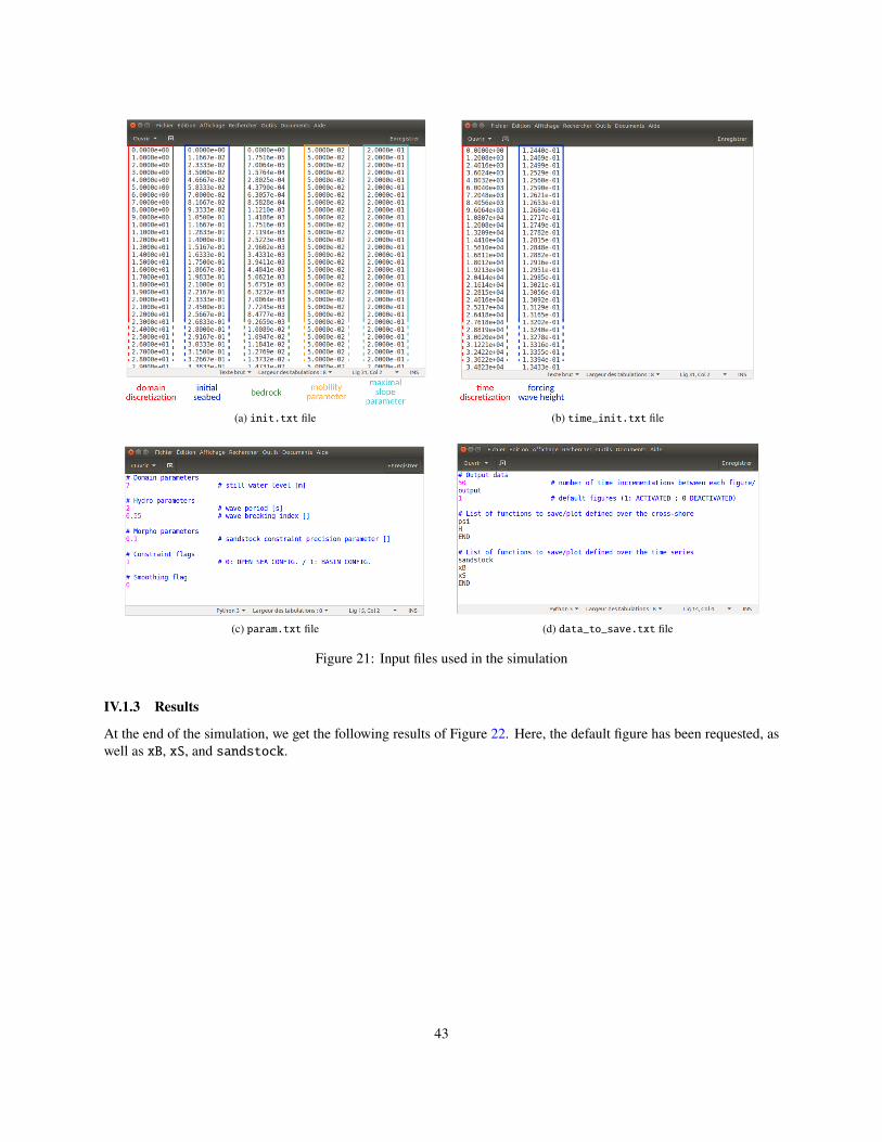
(a) init.txt file (b) time_init.txt file
(c) param.txt file (d) data_to_save.txt file
Figure 21: Input files used in the simulation
IV.1.3 Results
At the end of the simulation, we get the following results of Figure 22. Here, the default figure has been requested, aswell as xB, xS, and sandstock.
43

(a) Result of the beach configuration at the end of simulation
(b) Variation of the breaking point over time (c) Variation of the shoreline over time (d) Variation of the sandstock over time
Figure 22: Various plots provided by Opti-Morph
A thorough analysis of the results of Opti-Morph can be found in [Cook et al., 2021b] for an experimental flumeconfiguration and [Cook et al., 2021a] for a linear seabed with submerged breakwaters.
IV.2 Beach Configuration with submerged breakwatersIV.2.1 Setting
In this simulation, we introduce a solid submerged structure, in the same manner as [Cook et al., 2021a]. To do this,we modify the seabed profile, as well as the sand mobility parameter Υ and the maximal slope parameter "slope, whichare no longer constant over the cross-shore profile. In the case of the mobility parameter, no movement can occur atthe location of the structures, i.e. Υ = 0 where the breakwater is positioned. Similarly, the maximal slope parameterhas also been modified to locally deactivate the slope constraint over the structure. Figure 23 shows the new initialconfiguration incorporating a submerged breakwater located at G = 180<.
44

Figure 23: Initial sandy beach configuration with a submerged breakwater located at G = 180<
IV.2.2 Input files
Similar to before, the input files have been constructed, with Figure 21 providing an overview of the different files.Now, the mobility parameter Υ and the slope parameter "slope vary over the cross-shore profile.
45

(a) init.txt file (b) time_init.txt file
(c) param.txt file (d) data_to_save.txt file
Figure 24: Input files used in the simulation
A thorough analysis of the behavior of Opti-Morph in regards to the introduction of geotubes can be found in[Cook et al., 2021a].
IV.2.3 Results
At the end of the simulation, we get the following results of Figure 25. As before, the default figure has been activated(default_out = 1), and the graphs of xB, xS, and sandstock were requested.
46

(a) Result of the beach configuration with submerged breakwaters at the end of simulation
(b) Variation of the breaking point over time (c) Variation of the shoreline over time (d) Variation of the sandstock over time
Figure 25: Various plots provided by Opti-Morph
47
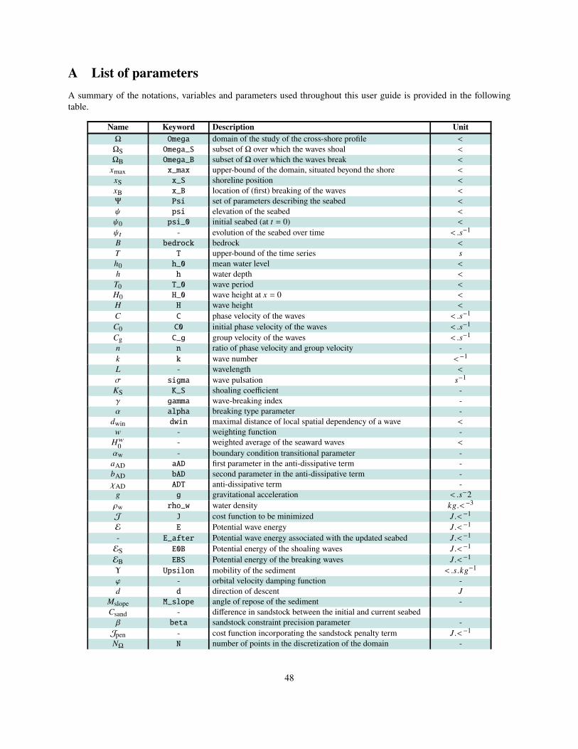
A List of parametersA summary of the notations, variables and parameters used throughout this user guide is provided in the followingtable.
Name Keyword Description UnitΩ Omega domain of the study of the cross-shore profile <
ΩS Omega_S subset of Ω over which the waves shoal <
ΩB Omega_B subset of Ω over which the waves break <
Gmax x_max upper-bound of the domain, situated beyond the shore <
GS x_S shoreline position <
GB x_B location of (first) breaking of the waves <
Ψ Psi set of parameters describing the seabed <
k psi elevation of the seabed <
k0 psi_0 initial seabed (at C = 0) <
kC - evolution of the seabed over time <.B−1
� bedrock bedrock <
) T upper-bound of the time series B
ℎ0 h_0 mean water level <
ℎ h water depth <
)0 T_0 wave period <
�0 H_0 wave height at G = 0 <
� H wave height <
� C phase velocity of the waves <.B−1
�0 C0 initial phase velocity of the waves <.B−1
�g C_g group velocity of the waves <.B−1
= n ratio of phase velocity and group velocity -: k wave number <−1
! - wavelength <
f sigma wave pulsation B−1
S K_S shoaling coefficient -W gamma wave-breaking index -U alpha breaking type parameter -3win dwin maximal distance of local spatial dependency of a wave <
F - weighting function -�F0 - weighted average of the seaward waves <
Uw - boundary condition transitional parameter -0AD aAD first parameter in the anti-dissipative term -1AD bAD second parameter in the anti-dissipative term -jAD ADT anti-dissipative term -6 g gravitational acceleration <.B−2dw rho_w water density :6.<−3
J J cost function to be minimized �.<−1
E E Potential wave energy �.<−1
- E_after Potential wave energy associated with the updated seabed �.<−1
ES E0B Potential energy of the shoaling waves �.<−1
EB EBS Potential energy of the breaking waves �.<−1
Υ Upsilon mobility of the sediment <.B.:6−1
i - orbital velocity damping function -3 d direction of descent �
"slope M_slope angle of repose of the sediment -�sand - difference in sandstock between the initial and current seabedV beta sandstock constraint precision parameter -Jpen - cost function incorporating the sandstock penalty term �.<−1
#Ω N number of points in the discretization of the domain -
48

#) - number of points in the discretization of the time series -(G?)?∈[0,#Ω ] x discretization of the domain Ω -(C?)?∈[0,#) ] t discretization of time interval [0, )] of the simulation -
- nbB position of GB in the discretization of the domain Ω -- nbS position of GS in the discretization of the domain Ω -- sandc flag activating the sandstock constraint -- smoothf flag activating a smoothing effect on the seabed -- T_out number of time steps between output -- default_out flag activating the creation of the default figure output -- CF0 choice of direction of descent �
References[Bouharguane et al., 2010] Bouharguane, A., Azerad, P., Bouchette, F., Marche, F., and Mohammadi, B. (2010).
Low complexity shape optimization and a posteriori high fidelity validation. Discrete and Continuous DynamicalSystems-series B - DISCRETE CONTIN DYN SYS-SER B, 13.
[Cook et al., 2021a] Cook, M., Bouchette, F., Mohammadi, B., and Fraysse, N. (2021a). Application of Opti-Morph:Optimized beach protection by submerged geotextile tubes. Preprint.
[Cook et al., 2021b] Cook, M., Bouchette, F., Mohammadi, B., Meulé, S., and Fraysse, N. (2021b). Opti-Morph, anew platform for sandy beach dynamics by constrained wave energy minimization. preprint.
[Cook et al., 2021c] Cook, M., Bouchette, F., Mohammadi, B., Sprunck, L., and Fraysse, N. (2021c). Optimal portdesign minimizing standing waves with a posteriori long term shoreline sustainability analysis. preprint.
[Dean and Dalrymple, 1991] Dean, R. G. and Dalrymple, R. A. (1991). Water Wave Mechanics for Engineers andScientists. WORLD SCIENTIFIC.
[Griewank and Walther, 2008] Griewank, A. and Walther, A. (2008). Evaluating Derivatives: Principles and Tech-niques of Algorithmic Differentiation. Society for Industrial and Applied Mathematics, second edition.
[Hascoët and Pascual, 2004] Hascoët, L. and Pascual, V. (2004). TAPENADE 2.1 user’s guide. Technical ReportRT-0300, INRIA.
[Isèbe et al., 2008a] Isèbe, D., Azerad, P., Bouchette, F., Ivorra, B., and Mohammadi, B. (2008a). Shape optimizationof geotextile tubes for sandy beach protection. International Journal for Numerical Methods in Engineering,74(8):1262–1277.
[Isèbe et al., 2008b] Isèbe, D., Azerad, P., Mohammadi, B., and Bouchette, F. (2008b). Optimal shape design ofdefense structures for minimizing short wave impact. Coastal Engineering, 55(1):35–46.
[Mohammadi and Bouchette, 2014] Mohammadi, B. and Bouchette, F. (2014). Extreme scenarios for the evolution ofa soft bed interacting with a fluid using the value at risk of the bed characteristics. Computers and Fluids, 89:78–87.
[Mohammadi and Bouharguane, 2011] Mohammadi, B. and Bouharguane, A. (2011). Optimal dynamics of softshapes in shallow waters. Computers and Fluids, 40:291–298.
[Munk, 1949] Munk, W. (1949). The solitary wave theory and its application to surf problems. Annals of the NewYork Academy of Sciences, 51:376 – 424.
[Soulsby, 1987] Soulsby, R. (1987). Calculating bottom orbital velocity beneath waves. Coastal Engineering - COASTENG, 11:371–380.
49