meditations on ceva’s theorem - lehrstuhl - webhome · pdf filetwo lines in the real...
TRANSCRIPT

Fields Institute Communications
Volume 00, 0000
Meditations on Ceva’s Theorem
Jurgen Richter-GebertTechnical University Munich
Zentrum MathematikBoltzmannstr. 3
D-85748 GarchingGermany
This paper is dedicated to the unforgettable H. S. M. Coxeter,who had a striking ability to relate visual thinking to formal notions
Abstract. This paper deals with the structure of incidence theoremsin projective geometry. We will show that many of these incidencetheorems can be interpreted as cyclic structures on a suitably chosenorientable manifold. Here the theorems of Ceva and Menelaus play theroles of basic building blocks for building larger theorems with greatercomplexity. In particular, we show how some other proofs for incidencetheorems can be systematically translated into such “Ceva/Menelaus-proofs”.
0 Introduction
Classical projective geometry was a beautifulfield in mathematics. It died, in our opinion,not because it ran out of theorems to prove,but because it lacked organizing principles bywhich to select theorems that were important.
R. MacPherson, M. McConnell, 1988 [17]
A “proof” is something where many things come together and in the end everythingcloses up nicely to form a conclusion. In this paper we will see that this verynaıve view of mathematical proofs is almost literally correct for certain classes ofgeometric incidence theorems. We will show that by a certain pasting process manynon-trivial incidence theorems can be generated by gluing many copies of Ceva and
1991 Mathematics Subject Classification. Primary 51A20, 51A05; Secondary 05B30, 52C35.
c©0000 American Mathematical Society
1
2 Jurgen Richter-Gebert
Menelaus configurations. These small building blocks are arranged at the faces ofa manifold and the final conclusion of the theorem corresponds to the fact that themanifold is topologically closed.The article deals with three different aspects of this construction principle.
• It will be shown how one can systematically generate incidence theorems bypasting together basic building blocks.
• We will see how a given incidence theorem can be analyzed and an underlyingmanifold structure can be revealed.
• It will be shown how to translate other proving techniques (in particular bi-quadratic final polynomials, as introduced in [5, 8, 18]) into Ceva/Menelausproofs. For this translation process the theory of Tutte Groups, as intro-duced by Dress and Wenzel in a series of papers [9, 10, 11, 22] plays a decisiverole.
• Finally, we will see how surgery on the manifolds, which underly the proofs,can be used, to generate even spaces of theorems.
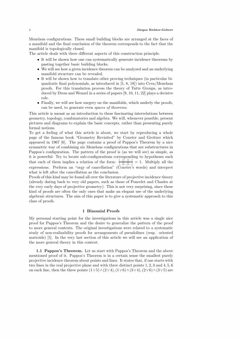
This article is meant as an introduction to these fascinating interrelations betweengeometry, topology, combinatorics and algebra. We will, whenever possible, presentpictures and diagrams to explain the basic concepts, rather than presenting purelyformal notions.To get a feeling of what this article is about, we start by reproducing a wholepage of the famous book “Geometry Revisited” by Coxeter and Greitzer whichappeared in 1967 [6]. The page contains a proof of Pappos’s Theorem by a nicesymmetric way of combining six Menelaus configurations that are substructures inPappos’s configuration. The pattern of the proof is (as we will see) as simple, asit is powerful: Try to locate sub-configurations corresponding to hypotheses such
that each of them implies a relation of the form: [...][...][...][...][...][...] = 1. Multiply all the
expressions. Perform an “orgy of cancellation” (Coxeter’s words) and interpretwhat is left after the cancellation as the conclusion.Proofs of this kind may be found all over the literature of projective incidence theory(already dating back to very old papers, such as those of Poncelet and Chasles atthe very early days of projective geometry). This is not very surprising, since thesekind of proofs are often the only ones that make an elegant use of the underlyingalgebraic structures. The aim of this paper is to give a systematic approach to thisclass of proofs.
1 Binomial Proofs
My personal starting point for the investigations in this article was a single niceproof for Pappos’s Theorem and the desire to generalize the pattern of the proofto more general contexts. The original investigations were related to a systematicstudy of non-realizability proofs for arrangements of pseudolines (resp. orientedmatroids) [5]. In the very last section of this article we will see an application ofthe more general theory in this context.
1.1 Pappos’s Theorem. Let us start with Pappos’s Theorem and the abovementioned proof of it. Pappos’s Theorem is in a certain sense the smallest purelyprojective incidence theorem about points and lines. It states that, if one starts withtwo lines in the real projective plane and with three distinct points 1, 2, 3 and 4, 5, 6on each line, then the three points (1∨5)∧(2∨4), (1∨6)∧(3∨4), (2∨6)∧(3∨5) are

Meditations on Ceva’s Theorem 3
Coxeter/Greitzer’s proof of Pappos’s Theorem.
automatically collinear as well. There are many different proofs for this fundamentaltheorem. We will consider a particularly well structured one. The theorem couldbe restated in the following way: If in RP
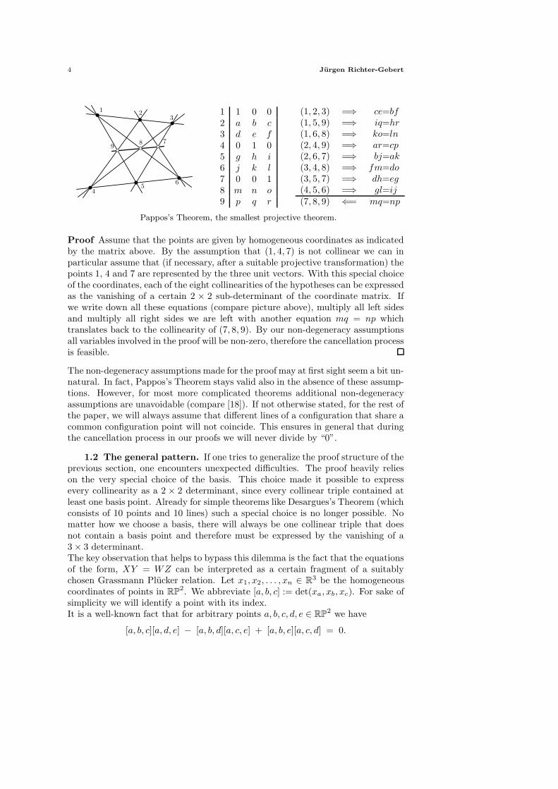
2 the triples of points (1, 2, 3), (1, 5, 9),(1, 6, 8), (2, 4, 9), (2, 6, 7), (3, 4, 8), (3, 5, 7), (4, 5, 6) are collinear, then (7, 8, 9) iscollinear as well.We give a proof of the theorem under the additional non-degeneracy assump-tions that no two lines of the picture coincide and that furthermore (1, 4, 7) isnot collinear.
4 Jurgen Richter-Gebert
PSfrag replacements
13
7
6
4
2
5
98
1 1 0 02 a b c3 d e f4 0 1 05 g h i6 j k l7 0 0 18 m n o9 p q r
(1, 2, 3) =⇒ ce=bf(1, 5, 9) =⇒ iq=hr(1, 6, 8) =⇒ ko=ln(2, 4, 9) =⇒ ar=cp(2, 6, 7) =⇒ bj=ak(3, 4, 8) =⇒ fm=do(3, 5, 7) =⇒ dh=eg(4, 5, 6) =⇒ gl=ij(7, 8, 9) ⇐= mq=np
Pappos’s Theorem, the smallest projective theorem.
Proof Assume that the points are given by homogeneous coordinates as indicatedby the matrix above. By the assumption that (1, 4, 7) is not collinear we can inparticular assume that (if necessary, after a suitable projective transformation) thepoints 1, 4 and 7 are represented by the three unit vectors. With this special choiceof the coordinates, each of the eight collinearities of the hypotheses can be expressedas the vanishing of a certain 2 × 2 sub-determinant of the coordinate matrix. Ifwe write down all these equations (compare picture above), multiply all left sidesand multiply all right sides we are left with another equation mq = np whichtranslates back to the collinearity of (7, 8, 9). By our non-degeneracy assumptionsall variables involved in the proof will be non-zero, therefore the cancellation processis feasible.
The non-degeneracy assumptions made for the proof may at first sight seem a bit un-natural. In fact, Pappos’s Theorem stays valid also in the absence of these assump-tions. However, for most more complicated theorems additional non-degeneracyassumptions are unavoidable (compare [18]). If not otherwise stated, for the rest ofthe paper, we will always assume that different lines of a configuration that share acommon configuration point will not coincide. This ensures in general that duringthe cancellation process in our proofs we will never divide by “0”.
1.2 The general pattern. If one tries to generalize the proof structure of theprevious section, one encounters unexpected difficulties. The proof heavily relieson the very special choice of the basis. This choice made it possible to expressevery collinearity as a 2 × 2 determinant, since every collinear triple contained atleast one basis point. Already for simple theorems like Desargues’s Theorem (whichconsists of 10 points and 10 lines) such a special choice is no longer possible. Nomatter how we choose a basis, there will always be one collinear triple that doesnot contain a basis point and therefore must be expressed by the vanishing of a3 × 3 determinant.The key observation that helps to bypass this dilemma is the fact that the equationsof the form, XY = WZ can be interpreted as a certain fragment of a suitablychosen Grassmann Plucker relation. Let x1, x2, . . . , xn ∈ R3 be the homogeneouscoordinates of points in RP
2. We abbreviate [a, b, c] := det(xa, xb, xc). For sake ofsimplicity we will identify a point with its index.It is a well-known fact that for arbitrary points a, b, c, d, e ∈ RP
2 we have
[a, b, c][a, d, e] − [a, b, d][a, c, e] + [a, b, e][a, c, d] = 0.
Meditations on Ceva’s Theorem 5
If in addition (a, b, c) is collinear, then we have automatically [a, b, c] = 0 and this,together with the Grassmann Plucker relation, implies the binomial equation
[a, b, d][a, c, e] = [a, b, e][a, c, d].
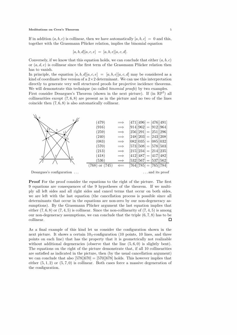
Conversely, if we know that this equation holds, we can conclude that either (a, b, c)or (a, d, e) is collinear since the first term of the Grassmann Plucker relation thenhas to vanish.In principle, the equation [a, b, d][a, c, e] = [a, b, e][a, c, d] may be considered as akind of coordinate free version of a 2×2 determinant. We can use this interpretationdirectly to generate very well structured proofs for projective incidence theorems.We will demonstrate this technique (so called binomial proofs) by two examples.First consider Desargues’s Theorem (shown in the next picture). If (in RP
2) allcollinearities except (7, 6, 8) are present as in the picture and no two of the linescoincide then (7, 6, 8) is also automatically collinear.
PSfrag replacements
6
1
8
3
9
7
5
0
2
4
(479) =⇒ [471][496] = [476][491](916) =⇒ [914][962] = [912][964](259) =⇒ [256][291] = [251][296](240) =⇒ [248][203] = [243][208](083) =⇒ [082][035] = [085][032](570) =⇒ [573][508] = [578][503](213) =⇒ [215][234] = [214][235](418) =⇒ [412][487] = [417][482](536) =⇒ [532][567] = [537][562]
(768) or (745) ⇐= [764][785] = [765][784]
Desargues’s configuration . . . . . . and its proof
Proof For the proof consider the equations to the right of the picture. The first9 equations are consequences of the 9 hypotheses of the theorem. If we multi-ply all left sides and all right sides and cancel terms that occur on both sides,we are left with the last equation (the cancellation process is possible since alldeterminants that occur in the equations are non-zero by our non-degeneracy as-sumptions). By the Grassmann Plucker argument the last equation implies thateither (7, 6, 8) or (7, 4, 5) is collinear. Since the non-collinearity of (7, 4, 5) is amongour non-degeneracy assumptions, we can conclude that the triple (6, 7, 8) has to becollinear.
As a final example of this kind let us consider the configuration shown in thenext picture. It shows a certain 103-configuration (10 points, 10 lines, and threepoints on each line) that has the property that it is geometrically not realizablewithout additional degeneracies (observe that the line (5, 6, 0) is slightly bent).The equations on the right of the picture demonstrate that, if all 10 collinearitiesare satisfied as indicated in the picture, then (by the usual cancellation argument)we can conclude that also [578][670] = [570][678] holds. This however implies thateither (5, 1, 2) or (5, 7, 0) is collinear. Both cases force a massive degeneration ofthe configuration.

6 Jurgen Richter-Gebert
PSfrag replacements
12
3
4
56
7
8
9
0
(129) =⇒ [128][179] = +[127][189](136) =⇒ [146][130] = −[134][160](148) =⇒ [124][168] = −[128][146](235) =⇒ [234][250] = −[245][230](247) =⇒ [127][245] = −[124][257](304) =⇒ [134][230] = +[130][234](056) =⇒ [160][570] = +[150][670](759) =⇒ [157][789] = −[179][578](869) =⇒ [189][678] = −[168][789](780) =⇒ [578][670] = +[570][678]
[157][250] = +[150][257]
A non-realizable 103 configuration.
1.3 Automatic proving. The above proving technique was successfully ap-plied in [8, 18] to create algorithms that prove many theorems in projective geom-etry automatically. The algorithm has the particularly nice feature that, if it findsa proof, the proof admits a clear readable structure, such that its correctness canbe checked by hand easily. This is an interesting contrast to automatic provingtechniques that are based on methods of commutative algebra (like Grobner Basisor Ritt’s algebraic decomposition method) that produce proofs consisting of largepolynomials of generally high degree.The basic idea of such a binomial-based proving algorithm is simple. First onegenerates all binomial relations that are consequences of the hypotheses of thetheorem. Then one creates binomial expressions that imply the conclusion andfinally tests whether one of the conclusion binomials can be generated as a suitablecombination of the hypotheses binomials. In fact, this last step can be carried out,in principle, by a linear equation solver, since one is interested in linear combinationsof the exponent vectors. In this approach the determinants themselves are treatedas formal symbols (variables) and one has never to go down to the concrete levelof coordinates.Although this method has the potential to find nice and well structured proofs ofthis kind, if they exist, it has a great disadvantage. When in the third step thelinear equation solver searches for a suitable dependence it has “forgotten” all struc-tural information about the theorem. In essence it searches “blindly” for a lineardependence in a space in which the variables correspond to the
(
n3
)
determinants,and where each collinearity corresponds to many binomial equations. Since thecalculations all have to be carried out in exact arithmetic, one may easily run intospace or time problems. It would be much more desirable to have some insight inthe possible structures of such proofs to rule out many unreasonable cancellationpatterns in advance. This is what the rest of this paper is about.
2 Theorems on manifolds
In this section we will give a different view on cancellation patterns that can beused to prove incidence theorems. The cancellation pattern used now will have theadditional feature that it can be interpreted directly in a topological way.

Meditations on Ceva’s Theorem 7
2.1 The theorems of Ceva and Menelaus. We will sketch a remarkablerelation between incidence theorems and cycles on manifolds. At first sight thepresented approach to incidence theorems seems to be very special but indeed wewill demonstrate in Section 6 that this approach is as expressive as the binomialproofs described in the previous section.Our main protagonists are the theorems of Ceva and of Menelaus. Ceva’s Theoremstates that if in a triangle the sides are cut by three concurrent lines that passthrough the corresponding opposite vertex, then the product of the three (oriented)length ratios along each side equals 1. Menelaus’s Theorem states that this productis −1 if the cuts along the sides come from a single line.
PSfrag replacements
A B
C
Z
YD
XX
PSfrag replacements
A B
C
Z
Y
DX
X
Ceva’s Thm: |AX||XB|
·
|BY ||Y C|
·
|CZ||ZA|
= 1 Menelaus’s Thm: |AX||XB|
·
|BY ||Y C|
·
|CZ||ZA|
= −1
In fact, these theorems are almost trivial if one views the length ratios as ratios ofcertain triangle areas. For this observe that, if the line (A, B) is cut by the line(C, D) at a point X , then we have
|AX |
|XB|= −
∆(C, D, A)
∆(C, D, B), (∗)
where ∆(A, B, C) denotes the oriented triangle area.
In order to prove Ceva’s Theorem we consider the obvious identity:
∆(CDA)
∆(CDB)·∆(ADB)
∆(ADC)·∆(BDC)
∆(BDA)= −1,
(note that the triangle area ∆ is an alternating function and that each triangle inthe denominator occurs as well in the numerator). Applying the above identity (∗)we immediately get Ceva’s Theorem. Similarly, a proof of Menelaus’s Theorem isderived. For this consider the special line as being generated by two points D andE. We have
∆(DEA)
∆(DEB)·∆(DEB)
∆(DEC)·∆(DEC)
∆(DEA)= 1,
Applying the identity (∗) yields Menelaus’s Theorem. Observe that the expressionsof Ceva and Menelaus carry an orientation information. If in the future we talkabout the “Ceva-expression” (or “Menelaus-expression”) for the triangle A, B, Cthe letters A, B, and C are assumed to be ordered as in the expression above.A, C, B would generate the reciprocal expression. Furthermore, we will call thepoints X , Y , and Z in the above drawing the edge points of the configuration.The points A, B, and C will be called the vertices of the configuration. Point D inCeva’s configuration will be called the Ceva point and the cutting line in Menelaus’sconfiguration is the Menelaus line.

8 Jurgen Richter-Gebert
2.2 A homotopy argument. Now, consider the situation where two trian-gles that are equipped with a Ceva configuration share an edge and the correspond-ing edge point on this edge (see the picture below). The triangle A, B, C yields a
relation |AZ||ZB| ·
|BX||XC| ·
|CY ||Y A| = 1 while the triangle C, B, D yields |CX|
|XB| ·|BV ||V D| ·
|DW ||Y W | = 1.
The quotient |BX||XC| occurs in the first expression and its reciprocal occurs in the sec-
ond expression. If we multiply both expressions, this quotient cancels and we areleft only with terms that live on the boundary of the figure. We obtain
|AZ|
|ZB|·|CY |
|Y A|·|BV |
|V D|·|DW |
|Y W |= 1.
We now consider a triangulated topological disc. All triangles of the triangulationshould be equipped with Ceva configurations that have the additional property thatpoints on interior edges are the shared edge points of the two adjacent triangles.We consider the product of all corresponding Ceva-expressions.
PSfrag replacements A
C
B
D
X
Y
Z
V
W
PSfrag replacementsACBDXYZVW
a1
b1
a2
b2
a3b3
a4
b4
a5
b5
a6
b6
Gluing two Ceva Configutarions Gluing many Ceva Configutarions
If the triangles are oriented consistently (adjacent triangles use the common edgein opposite directions), all quotients related to inner edges will cancel. We areleft with an expression that only depends on the position of the boundary points(including the edge points along the boundary edges). If in the last picture on theright the letters a1, b1, , . . . , a6, b6 correspond to the oriented lengths around theboundary we can conclude immediately that we must have
a1
b1·a2
b2·a3
b3·a4
b4·a5
b5·a6
b6= 1.
Now, consider any triangulated manifold that forms an oriented 2-cycle. Thiscycle serves as a kind of frame for the construction of an incidence theorem. Itis important to mention in what category we understand the term “triangulatedmanifold”. We consider compact, orientable 2 manifolds without boundary andsubdivisions by CW-complexes whose faces are triangles. So in principle, alreadya subdivision of a 2-sphere by two topological triangles, which are identified alongthe edges, would be a feasible object for our considerations.Consider such a cycle as being realized by flat triangles (it does not matter ifthese triangles intersect, coincide or are coplanar as long as they represent thecombinatorial structure of the cycle). By the above argument the presence of Cevaconfigurations on all but one of the faces will imply automatically the existenceof a Ceva configuration on the final face. Thus at the final face the three lines

Meditations on Ceva’s Theorem 9
connecting the edge points and the vertices will meet automatically, and we havean incidence theorem. In what follows we will study many concrete examples ofthis amazingly rich construction technique.As a first example take the projection of a tetrahedron (ABCD) to R2. Now, choosePoints U, V, W, X, Y, Z one on each of the edges of the tetrahedron. Assume that forthree of the faces these points form a Ceva configuration. Then they automaticallyform a Ceva configuration on the last face — an incidence theorem.
PSfrag replacements
A C
D
B
U V
WX
Y
Z
+
PSfrag replacements
A C
D
B
U V
WX
Y
Z
=
PSfrag replacements
A C
D
B
U V
WX
Y Z
Although the proof of this incidence theorem is already evident by our above homo-topy argument, we still want to present the algebraic cancellation pattern in detail.Consider the following formula
(
|AU ||UB| ·
|BV ||V C| ·
|CY ||Y A|
)
·(
|CW ||WD| ·
|DX||XA| ·
|AY ||Y C|
)
·(
|AX||XD| ·
|DZ||ZB| ·
|BU ||UA|
)
·(
|BZ||ZD| ·
|DW ||WC| ·
|CV ||V B|
)
= 1.
This formula is obviously true, since all lengths of the numerator occur in thedenominator as well and vice versa (this property is inherited from the cyclic struc-ture). On the other hand, each of the factors in brackets being 1 states the Cevacondition for one of the faces. Thus three of these conditions imply the last one.The essential fact that makes this proof work is that whenever two faces meet inan edge the two corresponding ratios cancel. In general we obtain:
For any triangulated oriented 2-CW-cycle choose a point on each
edge such that for every face either a Ceva or a Menelaus condition
is generated. If altogether an even number of Menelaus configura-
tions is involved, then the conditions on all but one of the triangles
automatically imply the condition on the last triangle.
We need an even number of Menelaus configuration since each Menelaus configura-tion accounts for a factor of −1 in the product. We will call such a cycle equippedwith Ceva/Menelaus configurations a Ceva/Menelaus-cycle. Instead of drawing thewhole incidence structure we often simply draw a schematic diagram, in which weindicate the combinatorial structure of the cycle and attach a label C or M to eachof the faces. We will usually draw these schemes as a planar net of triangles forwhich we specify which vertices and which edges have to be identified.
3 A census of incidence theorems
At first instance the method described in the last section is very useful for pro-ducing geometric incidence theorems by pasting together triangles that carry Cevaor Menelaus configurations. In this chapter we want to elaborate on this aspect.

10 Jurgen Richter-Gebert
We will at least for small numbers of triangles list several examples that can beproduced by this philosophy. In any case we need a configuration of triangles thatforms a closed orientable CW-cycle. It may happen that two triangles are identifiedalong more than one edge. However, to avoid trivial cases (in which the two config-urations of these triangles together with the edge points simply coincide), we haveto assume that in such a case one triangle is equipped with a Ceva configurationand the other with a Menelaus configuration. Later on such a sub-configurationconsisting of two triangles that coincide along two edges will be called a “pocket”.Let us now start with a census of small incidence theorems. Observe that thenumber of triangles involved in a Ceva/Menelaus-cycle must be even.
3.1 Two triangles. For two triangles there is only one possibility of forminga Ceva/Menalaus-cycle. We can only identify the two triangles along their edges.Then we have to assign to one of the triangles a Ceva configuration and to the otherone a Menelaus configuration. In the real projective plane this configuration is notrealizable at all, since one triangle forces the product of ratios to be −1 the otherforces the product of ratios do be 1. However, if we consider a field of characteristictwo, then this configuration is an incidence theorem. In fact, this configurationis nothing else but the well-known Fano plane. In the triangle scheme below thelabels at the vertices of the triangles indicate which vertices have to be identified.
PSfrag replacements
1
2 3
1
C
M
The Fano configuration . . . . . . and its triangle scheme
3.2 Four triangles. The structure becomes considerably richer if we considerfour instead of only two triangles. First of all there are two combinatorially differ-ent ways of creating a manifold involving four triangles: either they could form atetrahedron, or they could form a manifold, in which two pockets formed by twotriangles are pasted. It is important to observe that for the last case one has notonly to make clear which vertices have to be identified, but also which edges (andwith them the edge points) have to be identified.
PSfrag replacements
1
2 3
43
3
A
A
B
B
C
C
CM
CM
PSfrag replacements
1
2 3
43
3
A
A
B
B
C
C
CM
MC
PSfrag replacements
1
32
44
4
M
M
M M
PSfrag replacements
1
32
44
4
M
M
C C
PSfrag replacements
1
32
44
4
C
C
C C
All five possibilities to form an incidence theorem on four triangles.

Meditations on Ceva’s Theorem 11
The first row shows the two possible cases for the “pocket” version. The secondrow shows the three possibilities of assigning Ceva and Menelaus configurations toa tetrahedron.Let us now analyze the geometric interpretation of these cases as incidence the-orems. The situation for the first example of the first row is shown in the nextpicture. In principle, two adjacent triangles that carry a Ceva configuration areoverlaid with two adjacent triangles that carry Menelaus configurations. The finalcoincidence of the resulting configuration is satisfied automatically. The resultingimage is the well-known configuration that shows that for three given points on aline one can construct a harmonic point by erecting a drawing of a tetrahedron overthe line.
+ =
Although the second picture in the first row is combinatorially different from thefirst one, the resulting incidence configuration is exactly the same. The patientreader is invited to check this.The first scheme in the second row is nothing else but a description of Desargues’sTheorem, which we already encountered in Section 1. The following picture showsthe decomposition of the tetrahedron in a front and a back part.
+ =
The last two theorems in the second row correspond to the incidence configurationsshown in the next picture. In fact, the last example is the one we already havestudied when we introduced the proving technique three pages earlier. This config-uration has a few remarkable special cases in which one or more points do coincide.

12 Jurgen Richter-Gebert
However, we will not analyze them here in detail.
3.3 Six triangles. Already with six triangles the situation becomes quiteelaborate. There are altogether six combinatorially different types of cycles, and21 different types of underlying incidence configurations. We will not list all ofthem here. Some of the manifolds involve “pocket” sub-configurations and will beconsidered in a more general setting later on in Section 4. The only cycles thatdo not contain pockets are shown in the next picture. The cycle on the left isa double pyramid over a triangle. There are 8 non-isomorphic ways to equip itwith Ceva and an even number of Menelaus configurations. We will not studythese cases here. The second cycle is topologically more interesting. It is thesmallest CW-decomposition of a torus into triangles. It has only three vertices andnine edges. There are exactly four ways of assigning a Ceva/Menelaus-cycle to it:all triangles Ceva, exactly two adjacent triangles Menelaus, exactly two adjacenttriangles Ceva, all triangles Menelaus. The next subsection will be dedicated to adetailed discussion of the first and the last one of these situations.
PSfrag replacements1
2 3
4
4
4
4
5
6A
A
B
B
C
C
D
D
PSfrag replacements
1
1
1
2
2
23
456 A
A B
B
C
C
D
3.4 Pappos revisited. We now will deal exclusively with the situation ofsix triangles that form a topological torus. First observe, that if we realize thiscycle by flat triangles, then the only way of doing this is by making all trianglescoincident. Assume the triangles are realized in this way and furthermore assumethat we assign a Ceva configuration to each of these triangles. The left drawingof the next picture shows the unfolded configuration, while the middle drawingshows the overlay. Observe that for each of the triangles we get one Ceva point.Lines of two adjacent triangles that share the corresponding edge point becomeidentified. So, all together we have the three original points of the triangle, and six
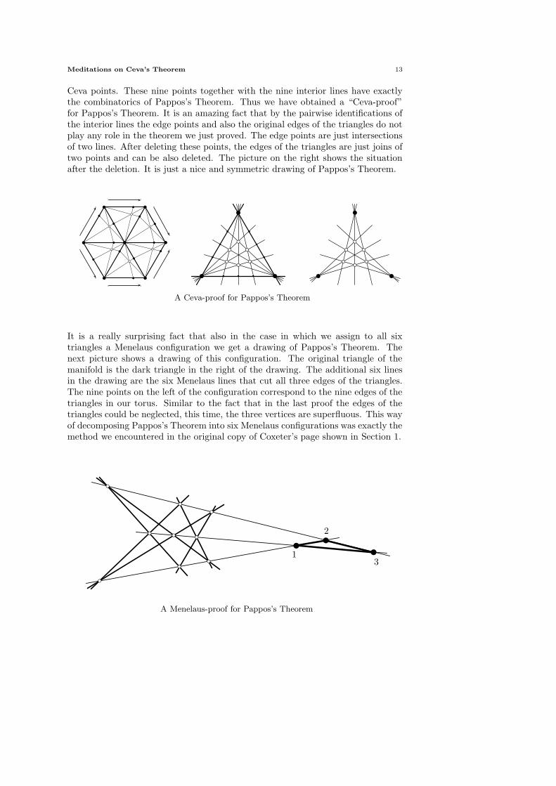
Meditations on Ceva’s Theorem 13
Ceva points. These nine points together with the nine interior lines have exactlythe combinatorics of Pappos’s Theorem. Thus we have obtained a “Ceva-proof”for Pappos’s Theorem. It is an amazing fact that by the pairwise identifications ofthe interior lines the edge points and also the original edges of the triangles do notplay any role in the theorem we just proved. The edge points are just intersectionsof two lines. After deleting these points, the edges of the triangles are just joins oftwo points and can be also deleted. The picture on the right shows the situationafter the deletion. It is just a nice and symmetric drawing of Pappos’s Theorem.
A Ceva-proof for Pappos’s Theorem
It is a really surprising fact that also in the case in which we assign to all sixtriangles a Menelaus configuration we get a drawing of Pappos’s Theorem. Thenext picture shows a drawing of this configuration. The original triangle of themanifold is the dark triangle in the right of the drawing. The additional six linesin the drawing are the six Menelaus lines that cut all three edges of the triangles.The nine points on the left of the configuration correspond to the nine edges of thetriangles in our torus. Similar to the fact that in the last proof the edges of thetriangles could be neglected, this time, the three vertices are superfluous. This wayof decomposing Pappos’s Theorem into six Menelaus configurations was exactly themethod we encountered in the original copy of Coxeter’s page shown in Section 1.
PSfrag replacements
1
2
3
A Menelaus-proof for Pappos’s Theorem

14 Jurgen Richter-Gebert
4 Basic building blocks
In this section we want to review a few basic substructures that are very oftenpresent in Ceva/Menelaus-proofs. In general, these basic substructures can bedirectly assigned to elementary principles of projective geometry – like cross ratios,harmonic points, or perspectives.
4.1 Pockets, . . .. In the last section we already encountered the situation inwhich two triangles were joined along two edges. In this case it was necessary toequip one of the triangles with a Ceva configuration and the other with a Menelausconfiguration (otherwise the third edge-point would coincide as well). In Section3.1 we already saw that we can identify the two triangles along the third line onlyin fields of characteristic 2. Here we study the case, in which we do not identifythe edge points on the third line. In this case we will have exactly four points onthis line: two original triangle edges, one Ceva-edge-point and one Menelaus-edge-point. The next picture (left) shows the corresponding incidence configuration.Topologically we can consider the pocket as a disk that is bounded by two edges1 − C − 2 and 2 − M − 1. If we multiply the Ceva and the Menelaus condition weimmediately get
|1C|
|C2|·|2M |
|M1|= −1.
In other words 1, 2, C and M are in harmonic position.
PSfrag replacements
1 2
3
5
6
4
C M
PSfrag replacements123564CM
1 2
6
4
3
5
M C
Accidentally, we can interpret exactly the same incidence configuration also theother way around. If we interchange the role of the points 3, . . . , 6 according to3 ↔ 6, 4 ↔ 5, 5 ↔ 4, 6 ↔ 3, we see that for the (old) triangle 1, 2, 6 we obtain aninterchanged role of the Ceva and the Menelaus edge point. This shows that if wehave a pocket in a Ceva/Menelaus-cycle, we can freely interchange the role of the“C” and the “M” on the pocket without changing the incidence configuration.
4.2 . . . tunnels, . . .. A very common situation in projective incidence the-orems is that “information” about a certain substructure is transfered from onepart of the configuration to another by projection. For instance, if four points ona line have a certain cross ratio, any projection of these points onto another linewill result in four points with the same cross ratio. We can perfectly model thissituation by suitable substructures of Ceva/Menelaus-cycles. Assume that we havea CW-triangulation of a manifold that is homeomorphic to S1× [0, 1] (a sphere withtwo holes). The boundary of this manifold consists of two disjoint circles. If eachtriangle is equipped with a Ceva or Menelaus configuration (such that the numberof Menelaus configuration is even), then the product of the length ratios along thefirst cycle must be identical to the product of the length ratios on the second (or its

Meditations on Ceva’s Theorem 15
inverse, depending on the orientation). Thus in a sense the configuration transfersinformation from the first boundary cycle to the second one.The smallest possible situation is shown in the next picture. It consists of 4 trianglesthat form a simple cycle. Combinatorially the situation is a tetrahedron, with twocuts along two opposite edges. The cycles consist just of two edges, each.
PSfrag replacements
A
A′
A
A′
B
B′
1 124 3
X
X ′
Y
Y ′
If the situation is as in the picture, then for the corresponding products of lengthratios we get:
|AX |
|XB|·|BY |
|Y A|=
|A′X ′|
|X ′B′|·|B′Y ′|
|Y ′A′|.
In other words, the configuration transfers the cross ration of A, B, X, Y to thepoints A′, B′, X ′, Y ′. If all triangles are equipped with Menelaus’s configurations,the corresponding incidence configuration is shown in the following picture (left).
PSfrag replacements
A
B
A′
B′X
Y
X ′
Y ′
1
2
3
4
PSfrag replacements
A
B
A′
B′X
Y
X ′
Y ′
1
2
3
4
The right picture shows a special instance of this configuration, in which the points1 and 2 (and several lines) coincide. In this picture the points A, B, X, Y andthe points A′, B′, X ′, Y ′ are connected to each other by a perspectivity. So weobtained a Ceva/Menelaus-proof for the fact that the cross ratios are preserved byperspectivities.
4.3 . . . and toothpicks. In this subsection we will study the semantics ofdegenerate Ceva triangles and degenerate Menelaus triangles. Usually, a Ceva
configuration produces a relation |AX||XB| ·
|BY ||Y C| ·
|CZ||ZA| = 1. This relation remains also
valid if the points A, B, C are collinear. In this case, however, the points X, Y, Zwill coincide with the vertices. And we will get:
|AC|
|CB|·|BA|
|AC|·|CB|
|BA|= 1.

16 Jurgen Richter-Gebert
PSfrag replacements
A B
C
X
ZY
PSfrag replacements
A B
C
X
ZY
Similarly, applying Menelaus’s Theorem to a degenerate triangle A, B, C we seethat the Menelaus line intersects the line A, B, C at a unique point X , since alledge points will coincide. In this case we get the identity
|AX |
|XB|·|BX |
|XC|·|CX |
|XA|= −1.
Here X can be any point on the line through A, B, C.One might wonder whether such degenerate configurations may ever occur in areal proof of an incidence theorem. From the point of view of Ceva/Menelaus
proofs the length ratios |AC||CB| must be considered as indecomposable units. The
degenerate subconfiguration gives us the possibility to replace |AC||CB| by the product
|CA||AB| ·
|AB||BC| . In particular, this gives us the possibility to exchange the role of edge
points and vertices. In fact, allowing degenerate triangles considerably broadensthe applicability of our proving methods. We want to discuss briefly how to derivea trivial (but useful) identity in a Ceva/Menelaus setup. Assume that A, B, X, Yare four points on a line. Then we obviously have:
|AX |
|XB|·|BY |
|Y A|=
|BY |
|XB|·|AX |
|Y A|.
However, if we consider the four length ratios as unbreakable symbols the identityis far from being trivial. We can establish this identity in our setup by pasting twodegenerate Ceva configurations (triangles A, B, X and A, B, Y ) and two degenerateMenelaus configurations (triangles X, Y, A and X, Y, B). The following calculationproofs the identity:
(
|AX||XB| ·
|BA||AX| ·
|XB||BA|
)
·(
|BY ||Y A| ·
|AB||BY | ·
|Y A||AB|
)
·(
|XB||BY | ·
|Y B||BA| ·
|AB||BX|
)
·(
|Y A||AX| ·
|XA||AB| ·
|BA||AY |
)
= 1.
Ratios that do not cancel are underlined. They yield exactly the desired expression.The combinatorics of this expression is again a kind of tunnel: A tetrahedron inwhich two holes are cut along opposite edges. If we close these two slots of thetetrahedron by two pockets, we immediately get a proof for the following incidencetheorem:
Meditations on Ceva’s Theorem 17
PSfrag replacementsA
BX Y
1
2
3 4
R
S
PSfrag replacementsABXY1234RS
R R
2 21 1
A AB
X Y
X
X
Y
A B
S S
3 34 4
ABA B B
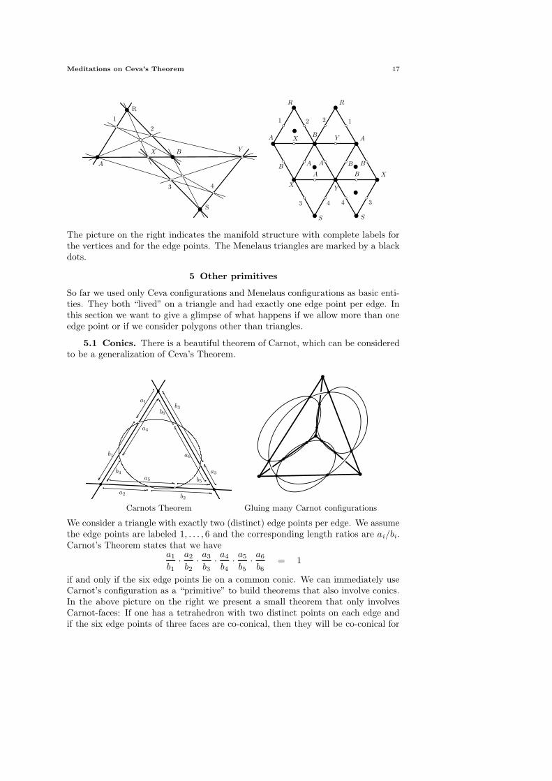
The picture on the right indicates the manifold structure with complete labels forthe vertices and for the edge points. The Menelaus triangles are marked by a blackdots.
5 Other primitives
So far we used only Ceva configurations and Menelaus configurations as basic enti-ties. They both “lived” on a triangle and had exactly one edge point per edge. Inthis section we want to give a glimpse of what happens if we allow more than oneedge point or if we consider polygons other than triangles.
5.1 Conics. There is a beautiful theorem of Carnot, which can be consideredto be a generalization of Ceva’s Theorem.
PSfrag replacements
a1
a2
a3
a4
a5
a6b1
b2
b3
b4
b5
b6
Carnots Theorem Gluing many Carnot configurations
We consider a triangle with exactly two (distinct) edge points per edge. We assumethe edge points are labeled 1, . . . , 6 and the corresponding length ratios are ai/bi.Carnot’s Theorem states that we have
a1
b1·a2
b2·a3
b3·a4
b4·a5
b5·a6
b6= 1
if and only if the six edge points lie on a common conic. We can immediately useCarnot’s configuration as a “primitive” to build theorems that also involve conics.In the above picture on the right we present a small theorem that only involvesCarnot-faces: If one has a tetrahedron with two distinct points on each edge andif the six edge points of three faces are co-conical, then they will be co-conical for

18 Jurgen Richter-Gebert
the last face automatically. In fact, there is nothing special about the tetrahedron.Any oriented triangulated 2-manifold would serve as a frame as well.It is also easily possible to prove, for instance, Pascal’s Theorem with this method.For this one combines one Carnot configuration with four Menelaus configurations.Since each edge of the Carnot configuration has two edge points, one has to countthem with multiplicity two and each of these edges has to be glued to two Menelausconfigurations – one for each edge point.
5.2 n-gons. If we consider n-gons instead of triangles we immediately canproduce several nice generalizations of Ceva’s and Menelaus’s Theorem. Many ofthem have been studied in the literature. Most of them are of the form that a certain(combinatorially symmetric) incidence configuration forces a certain product oflength ratios (often with cyclic symmetry) to be 1 or −1. For an extensive treatmentof this topic see the article series [12, 13, 14, 15, 21]. Here we only want to presentthree of these theorems, without proofs.
PSfrag replacements
A
B
C
D
W
X
Y
ZPSfrag replacements
A
B
C
DD
WW
X
Y
Z
O
PSfrag replacements
A
B
C
DD
W
WX
Y
Z
A lifting condition Hoehn’s Theorem General Menelaus
If we consider a quadrangle A, B, C, D (first picture above) with edge points W ,X , Y , Z, then the condition
|AW |
|WB|·|BX |
|XC|·|CY |
|Y D|·|DZ|
|ZA|= 1
holds if and only if the six lines of the picture are tangent to a common conic.Another equivalent condition for this is that there is a proper lifting of these linesto three-space that preserves all nine incidences.The second drawing shows a theorem which is known under the name Hoehn’sTheorem. Consider an n-gon with odd n and an additional point O. If we constructedge points by intersecting each edge with the line that connects O to the oppositevertex, then the cyclic product of the length ratios will be 1. This theorem isa direct generalization of Ceva’s Theorem where we have n = 3. It has to bementioned that the converse of Hoehn’s Theorem is not true for n > 3, since thecyclic product being 1 does not necessarily imply that all central lines meet in apoint (which can be seen by a simple degree-of-freedom count). One can prove thistheorem by exactly the same idea we used in Section 2.1 to prove Ceva’s Theorem.The last picture shows a generalization of Menelaus’s Theorem. Consider an n-gon where edge points are generated by cutting the edges with a single line (notnecessarily in the interior) then the cyclic product of the length ratios equals (−1)n.The theorem can be proved easily by triangulating the n-gon, applying the usualMenelaus Theorem to all triangles and canceling all interior edges.
Meditations on Ceva’s Theorem 19
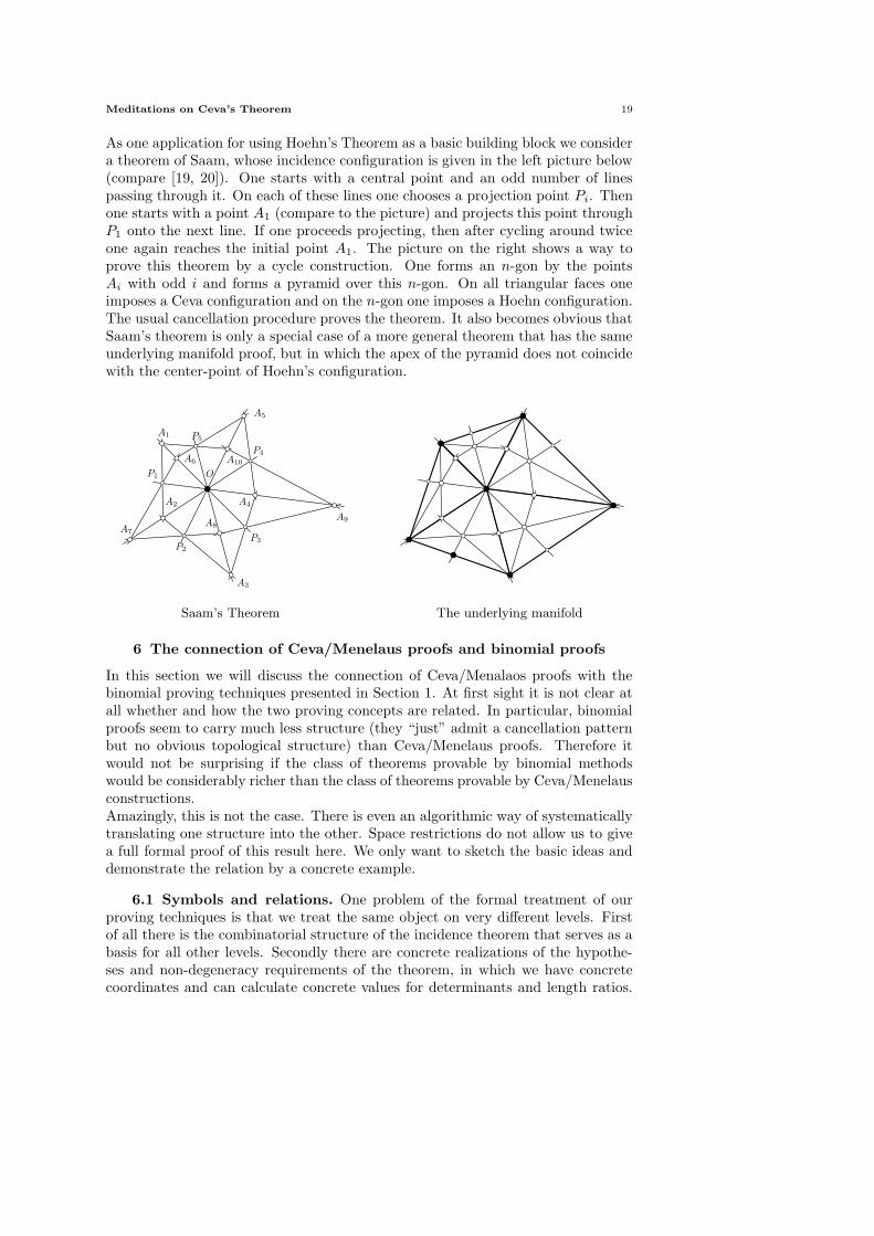
As one application for using Hoehn’s Theorem as a basic building block we considera theorem of Saam, whose incidence configuration is given in the left picture below(compare [19, 20]). One starts with a central point and an odd number of linespassing through it. On each of these lines one chooses a projection point Pi. Thenone starts with a point A1 (compare to the picture) and projects this point throughP1 onto the next line. If one proceeds projecting, then after cycling around twiceone again reaches the initial point A1. The picture on the right shows a way toprove this theorem by a cycle construction. One forms an n-gon by the pointsAi with odd i and forms a pyramid over this n-gon. On all triangular faces oneimposes a Ceva configuration and on the n-gon one imposes a Hoehn configuration.The usual cancellation procedure proves the theorem. It also becomes obvious thatSaam’s theorem is only a special case of a more general theorem that has the sameunderlying manifold proof, but in which the apex of the pyramid does not coincidewith the center-point of Hoehn’s configuration.
PSfrag replacements
OP1
P2
P3
P4
P5A1
A2
A3
A4
A5
A6
A7A8
A9
A10
Saam’s Theorem The underlying manifold
6 The connection of Ceva/Menelaus proofs and binomial proofs
In this section we will discuss the connection of Ceva/Menalaos proofs with thebinomial proving techniques presented in Section 1. At first sight it is not clear atall whether and how the two proving concepts are related. In particular, binomialproofs seem to carry much less structure (they “just” admit a cancellation patternbut no obvious topological structure) than Ceva/Menelaus proofs. Therefore itwould not be surprising if the class of theorems provable by binomial methodswould be considerably richer than the class of theorems provable by Ceva/Menelausconstructions.Amazingly, this is not the case. There is even an algorithmic way of systematicallytranslating one structure into the other. Space restrictions do not allow us to givea full formal proof of this result here. We only want to sketch the basic ideas anddemonstrate the relation by a concrete example.
6.1 Symbols and relations. One problem of the formal treatment of ourproving techniques is that we treat the same object on very different levels. Firstof all there is the combinatorial structure of the incidence theorem that serves as abasis for all other levels. Secondly there are concrete realizations of the hypothe-ses and non-degeneracy requirements of the theorem, in which we have concretecoordinates and can calculate concrete values for determinants and length ratios.

20 Jurgen Richter-Gebert
On the other hand, if we consider binomial proofs, the determinants play merelythe role of formal symbols. We will not assign specific values to them, but theincidence structure of the theorem determines rules how these formal symbols arerelated to each other. In the case of binomial proofs the decisive relations on thesymbols are given by the identities of the form [. . .][. . .] = [. . .][. . .] that are used inour proofs. If we consider Ceva/Menelaus proofs instead, the role of formal sym-bols is played by the ratios of oriented lengths. The existence of Ceva or Menelaussub-configurations is translated into the presence of relations among these lengthratios.The essence of our proofs is that the purely formal treatment of the symbols (formaldeterminants or formal length ratios) allows to conclude additional relations thathave to be present in every realization of the hypotheses configuration. The idea oftreating the abstract properties of an incidence configuration on a formal level in notat all new. In his article The bracket ring of combinatorial geometry [23] N. Whitediscusses extensively the ring structure of formal determinants that is imposed by anunderlying incidence structure. Similarly, in a series if articles on the Tutte Groupof a matroid [9, 10, 11, 22] A. Dress and W. Wenzel analyze the consequences ofincidence relations on the abstract multiplicative group on several formal kinds ofsymbols. The abstract symbols that are studied there are abstract determinants,ratios of (adjacent) abstract determinants, and abstract scalar products. For a fixedunderlying matroid each of these setups produces a group and the three groups arevery closely related. Up to isomorphism they just differ by a factor of Zk. Theisomorphism is not at all trivial and relies on homotopy arguments on so calledMaurer graphs [10, 16].It turns out that the essence of our proving techniques can be nicely expressed interms of Tutte groups and it turns out that the equivalence of binomial proofs andCeva/Menelaus proofs relies on the equivalence of the different setups for Tuttegroups. For reasons of space limitations we will not present the formal setup here,since it involves quite a lot of technical machinery. Rather than that we will explainthe basic concepts and describe the translation process by a concrete example.
6.2 Binomial proofs vs. Ceva/Menelaus proofs. For our explanationswe will make a few simplifying assumptions. We will assume that we study aconcrete incidence configuration with a concrete matroid underlying it. We restrictthe considerations to the rank 3 case only. The hypotheses (and the conclusion)of our theorem will be expressed by certain non-bases of the matroid. The non-degeneracies will result in the presence of certain bases of the matroid. In generalan incidence theorem will not determine the underlying matroid uniquely. Only apartial structure of it will be fixed by the hypotheses non-degeneracies. We willneglect this technical difficulty and assume that we have a fixed underlying matroidM with set of bases B.We consider the graph GM whose vertices correspond to the bases B and whoseedges are those pairs of bases that differ exactly by one element. We will identifyeach determinant that occurs in a binomial proof (and therefore will be a basis)with the corresponding vertex of GM. Assume that (1, 2, 3) are collinear and that[1, 2, x][1, 3, y] = [1, 2, y][1, 3, x] is a corresponding binomial equation. Bases in-volved in such a binomial equation correspond to a 4-cycle in GM without diagonaledges. We will call such a quadrangle a binomial quadrangle. A binomial quad-rangle with vertices (1, 2, x), (1, 3, y), (1, 2, y), (1, 3, x) is called degenerate if at least

Meditations on Ceva’s Theorem 21
one of the triples (1, 2, 3) or (1, x, y) is not a basis. If both triples are non-bases itis called pure.We will bicolor degenerate quadrangles, which correspond to binomial equations,such that the bases on the left of the equations are colored white and the baseson the right are colored black. A binomial proof now corresponds to a collectionof (bicolored) binomial degenerate quadrangles, such that in this collection eachvertex is as often colored black, as it is colored white.
PSfrag replacements
[12x]
[12y] [13y]
[13x]
PSfrag replacements
[12x]
[13x] [12x]
PSfrag replacements
[1xy]
[2xy] [3xy]
a binomial quadrangle a triangle of first kind a triangle of second kind
In the picture above the first drawing shows such a quadrangle with labeled basesfor the binomial relation [1, 2, x][1, 3, y] = [1, 2, y][1, 3, x]. In the graph GM there canbe exactly two combinatorially different types of triangles. They are represented bythe two labeled triangles in the picture above. In the context of Tutte groups thesetriangles are called triangle of first kind and triangle of second type, respectively.One of the fundamental properties of such bases graphs of matroids is that everycycle in the graph can be generated as a sum of triangles and of pure quadrangles(here sum is meant in the sense that if coinciding edges are added with oppositedirections, then they cancel each other). If the rank three matroid does not containloops or parallel elements, each cycle can even be considered as sum of trianglesonly. This result is the technical kernel of the fact that the different Tutte groupsare isomorphic up to a Zk-factor. It will also be our main tool for the translationof binomial proofs into Ceva/Menelaus proofs.
PSfrag replacements
A
C
B
DX
Y
Z
EF
V
WPSfrag replacements
A
C
B
D
X
Y
Z
EF
V
WPSfrag replacements
[BCE]
[ABE] [BEX ] [BFX ] [BDF ]
[CBD]
[CDF ][CFX ][CEX ][CAE]
(AEX) (CXB) (DFX)
PSfrag replacements
[BCE]
[ABE] [BEF ] [BDF ]
[CBD]
[CDF ][CEF ][CAE]
(AEF ) (DFE)
Bases graphs of glued Ceva configurations.
There is a close connection of triangles of first and second kind to Ceva’s andMenelaus’s configuration. For this we consider the bases as non-zero triangle areas

22 Jurgen Richter-Gebert
in our configuration. An oriented edge can be interpreted as a quotient of two suchtriangle areas. As explained in Section 2.1. such a quotient can also be consideredas a ratio of lengths on a line. The three ratios encoded by each of the two trianglesare exactly those ratios that we used in our original proofs of Ceva’s and Menelaus’sTheorem in Section 2.1.Now, let us study the situation where in a Ceva/Menelaus proof two triangles areglued along an edge. What does the corresponding situation in the bases graphs looklike? We will only elaborate on two situations; the rest is essentially analogous. Letus consider the situations shown in the picture on the preceeding page, where twoCeva configurations are joined. In each of the corresponding cases a substructureof the basis graph is shown. The quadrangles that are visible in the graphs areactually degenerate binomial quadrangles (the triple inside the quadrangle indicatesthe non-basis that is responsible for the degeneracy). Recall that the quadrangles
represent a relation of the form [1,a,x][1,a,y] = [1,b,x]
[1,b,y] . Both sides of the equation can be
interpreted as representing the same length ratio, however represented by differentarea quotients. The chains of quadrangles that occurs in the examples above serveas a kind of translator between the two Ceva triangles. They make sure that thearea ratios in one triangle really represent the same length ratio as the area ratioof the other triangle. If we consider the bases graph underlying a configurationthat admits a Ceva/Menalaus proof, we will find the following substructure. EachCeva or Menelaus configuration of the proof corresponds to a suitable triangle inthe graph. All edges of these triangles are paired by chains of degenerate binomialquadrangles (this chain may have length zero). The collection of binomial equationscorresponding to exactly these quadrangles forms a binomial proof of the theorem.This gives the translation of Ceva/Menelaus proofs into binomial proofs.Slightly more complicated is the translation of a binomial proof into a Ceva/Mene-laus proof. (this is not very surprising, since the second kind of proof carriesmuch more structural information). We will demonstrate the basic procedure byan example that shows essentially all important features. We revisit the theorembelow (recall Section 4.3) and consider a concrete proof that was generated by animplementation of an algorithm that produces binomial proofs.
PSfrag replacements
4
9
BA C
2
3
8 6
1
5
7
[239][19A] = [139][29A]
[134][24A] = [124][34A]
[124][2AB] = -[12B][24A]
[12B][13C] = [123][1BC]
[123][39C] = -[239][13C]
[139][34A] = [134][39A]
[29A][19B] = [19A][29B]
[29B][5AB] = [2AB][59B]
[568][69A] = [569][68A]
[67C][569] = [567][69C]
[56A][58B] = [568][5AB]
[678][7BC] = -[67C][78B]
[567][68A] = -[56A][678]
[39A][69C] = [39C][69A]
[1BC][79B] = [19B][7BC]
[58B][79B] = [78B][59B]
How can we derive a Ceva/Menelaus proof from such a given binomial proof? Howcan we reveal and reconstruct the manifold structure? Here we will give a kind

Meditations on Ceva’s Theorem 23
of cooking recipe without a formal explanation why this recipe works. As a firststep we reconstruct a suitable substructure of the underlying basis graph. For eachbinomial equation of the proof we form a quadrangle with bicolored vertices andlabel the vertices by the corresponding bases. The bases on the left sides of thebinomial equations will be colored white, the others will be colored black. Wethen try to stick the quadrangles together such that each white vertex meets itsblack counterpart (see picture below – capital letters on an exterior edge mean thatthis edge has to be identified with the corresponding edge labeled by the identicalletter). This will always be possible since it was the defining property of a binomialproof. We will now interpret the quadrangles as substructures that are used to linkCeva/Menelaus configurations. For each quadrangle we have to make a decisionwhich pair of opposite sides is considered as carrying the information of the lengthratio. In our picture we have drawn these edges slightly darkened (observe thatthere is a lot of freedom in this choice). If two quadrangles are attached to eachother, such that the two dark edges coincide we can neglect these two edges forthe further considerations. We can also neglect the non-darkened edges. We areleft with a collection of darkened edges that will form several edge-disjoint cycles.In our example we have seven such cycles: five triangles, one quadrangle and apentagon. The choice which pair of edges will be darkened has a great influence onthe number and size of cycles we will get. In our example we made this choice ina way that a maximum number of dark edges became identified and such that weget many small cycles.
678 567
569
24A34A39A
78B
7BC
67C
69C 69A
68A
678
567
56A568
139
39C13C1BC
12B 123 239
29A
29B
B9558B
568
56A
B5A2AB
12B
1BC
7BC
78B
58B59B
79B
19B
19A
134 124 12B
2AB
C
C
A
A
F
B
B
F D
E
D
E
ih
g
f
d
c
b
a
e
j
ihg
fd
cba
e
5
8 C
5
C A
5
A 8
A
C 2
A
2 1
8
A 9
9
A 1
9
1 2
9
2 Cj
9
C B
a5
8 C
b5
C
A
c5 A
8
d
A
C 2
eA
2
1
f8
A
9
g9
A 1
h9
1
2
i9
2Cj
9
C8
Now, Maurer’s homotopy theorem tells us, that each cycle can be decomposedinto triangles (perhaps for this we have to use new bases that are not alreadypresent in the substructure constructed so far. In our example this is not thecase). In our example the quadrangle can be decomposed into two triangles and thepentagon is decomposed into three triangles. The collection of all these trianglesforms the support for all our Ceva/Menelaus configurations that are needed fora Ceva/Menelaus proof. From the bases labels at the vertices of the graph wecan easily read off whether a triangle has to be a considered as a Ceva or as a

24 Jurgen Richter-Gebert
Menelaus configuration. In our example only the triangles labeled “c” and “h” carryCeva configurations (in fact they are toothpicks). All other triangles are Menelausconfigurations. We can also easily read off the vertices for each triangle. Finally,we can take all these triangles with vertices labelled by the corresponding pointsand can construct a closed and oriented manifold from them. In fact, the basicgluing structure is already given by the chaining quadrangles. However, we have tobe a little careful to assign the correct orientation to the Ceva configurations (inthe Ceva/Menelaus manifold this will be opposite to the picture of the quadranglecancellations.). In our example the resulting manifold (right lower picture) turnsout to be a sphere. This finishes the process of translating a binomial proof into aCeva/Menelaus proof.
7 Spaces of theorems
In this section we want to give a glimpse on another aspect of Ceva/Menelausproofs — namely how different proofs can be combined to form new proofs of morecomplicated theorems. We will study this in the simplest possible case, for whichindeed even a complete classification is possible.
7.1 Grid theorems. For this we now come back to a structure that we havealready met in Section 3.4, when we proved Pappos’s Theorem. We will study thoseincidence theorems for which the Ceva/Menelaus proof requires only Ceva trianglesand for which furthermore all Ceva triangles have the same vertices 1, 2, 3. Pappos’sTheorem was the smallest such example. In such a theorem we have three bundlesof lines each bundle passing through one of the three vertices. Each Ceva pointis met by one line of each bundle. Since the position of each line is uniquelydetermined by the length ratio of the corresponding Ceva point, there must be amanifold proof if the underlying incidence structure is a theorem. If we have amanifold proof for such a theorem, then adjacent triangles of the manifold musthave opposite orientation with respect to the triangle (1, 2, 3). In our configurationwe color the Ceva points that use one orientation white and the others black. Thecrucial condition for us to have a theorem is that along each line we have as manyblack points as we have white points. The picture below shows the situation forPappos’s Theorem. The drawing in the middle is the situation in which the verticesof the triangle were moved to the line at infinity. We can associate a matrix to thesituation that has an entry “+1” for every white point, a “-1” for every black pointand zero otherwise. Our theorem property now translates into the fact, that such amatrix has columns sums, row sums and sums in the north-east diagonal directionall zero.
0 +1 −1−1 0 +1+1 −1 0
Pappos’s Theorem and its underlying matrix
Meditations on Ceva’s Theorem 25
7.2 Spaces of incidence theorems. Now, conversely consider an n×n ma-trix with integer entries and column sums, row sums, north-east diagonal sumsbeing zero. Without loss of generality one can assume that at least one entry of thematrix is odd. If not, divide the matrix by a suitable power of two. The non-zeroentry of the matrix will be called its support. Take a triangle (1, 2, 3) as frame foran incidence configuration. Each row that has a support entry will correspond toa Ceva line through point 1, each column that contains a support entry will corre-spond to a Ceva line through point 2 and similarly each diagonal to a Ceva pointthrough point 3. The support entries of the matrix correspond to the Ceva points,in which the corresponding row, column and diagonal lines meet. By this construc-tion each support entry corresponds to a Ceva triangle that has to be counted witha multiplicity induced by the value of the matrix entry (the sign indicates the orien-tation). The cancellation pattern on the manifold is directly induced by the sum= 0property of the matrix. We can conclude that the Ceva configuration at the odd
support entry with value s must satisfy a relation(
|AX||XB| ·
|BY ||Y C| ·
|CZ||ZA|
)s
= 1 and
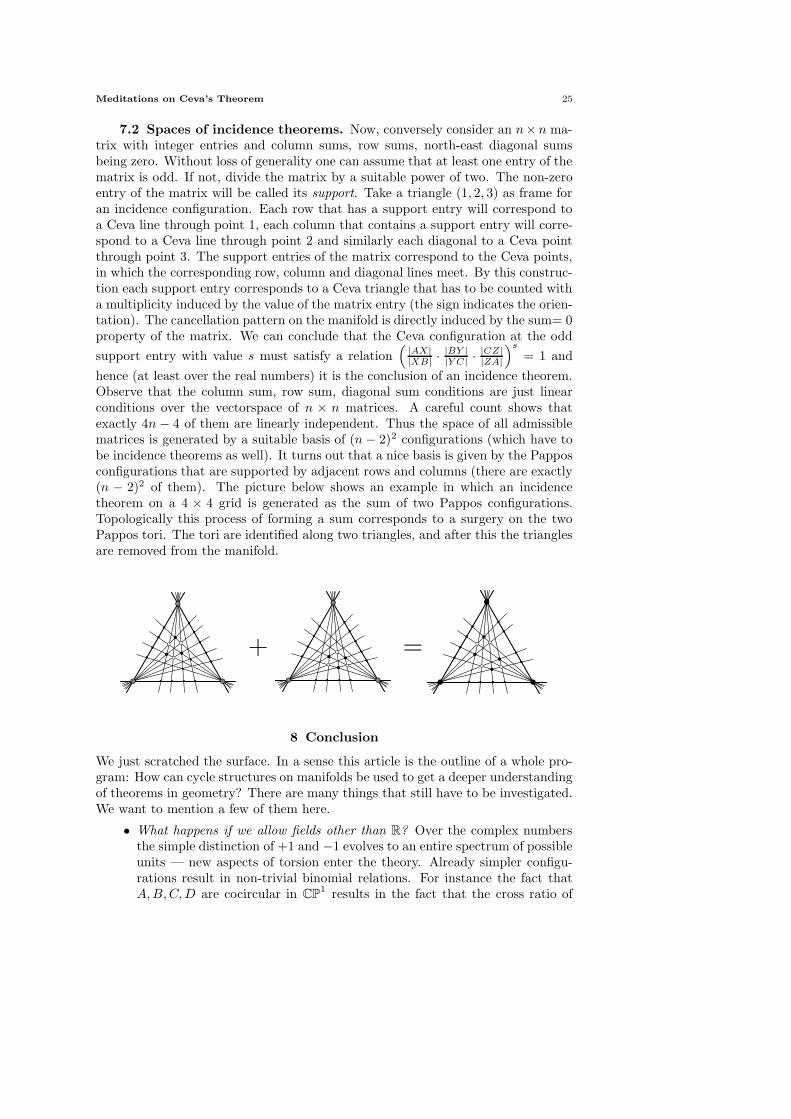
hence (at least over the real numbers) it is the conclusion of an incidence theorem.Observe that the column sum, row sum, diagonal sum conditions are just linearconditions over the vectorspace of n × n matrices. A careful count shows thatexactly 4n − 4 of them are linearly independent. Thus the space of all admissiblematrices is generated by a suitable basis of (n − 2)2 configurations (which have tobe incidence theorems as well). It turns out that a nice basis is given by the Papposconfigurations that are supported by adjacent rows and columns (there are exactly(n − 2)2 of them). The picture below shows an example in which an incidencetheorem on a 4 × 4 grid is generated as the sum of two Pappos configurations.Topologically this process of forming a sum corresponds to a surgery on the twoPappos tori. The tori are identified along two triangles, and after this the trianglesare removed from the manifold.
+ =
8 Conclusion
We just scratched the surface. In a sense this article is the outline of a whole pro-gram: How can cycle structures on manifolds be used to get a deeper understandingof theorems in geometry? There are many things that still have to be investigated.We want to mention a few of them here.
• What happens if we allow fields other than R? Over the complex numbersthe simple distinction of +1 and −1 evolves to an entire spectrum of possibleunits — new aspects of torsion enter the theory. Already simpler configu-rations result in non-trivial binomial relations. For instance the fact thatA, B, C, D are cocircular in CP
1 results in the fact that the cross ratio of

26 Jurgen Richter-Gebert
these points is real. It is an easy task to take such cross ratio quadran-gles and form manifolds from them that prove incidence theorems (see forinstance [2, 21]).
• What about second and third order syzygies? In this article we studied rela-tions among sub-configurations of an incidence theorem. In the last sectionwe saw that there are cases in which spaces of such theorems emerge. Whatcan we say about relations between these relations, or even about relationson the relations between the relations. At least in the context of the bracketring such problems have been partially studied [7].
• Back to non-realizability proofs. The origin of the whole investigations werenon-realizability proofs for arrangements of pseudolines. How can the re-sults in this paper, be applied to get classification results with respect torealizability and non-realizability in this context. In particular, realizabilityof pseudoline arrangements that consist of three bundles of pseudolines canbe characterized completely by the methods in Section 7. This implies alsoa characterization of liftable rhombic tilings with three directions.
• Where is the complexity? Proving theorems is provably hard. So the ques-tion arises about the limits of the proving techniques described here. Whatdo theorems look like, that cannot be proved by Ceva/Menelaus proofs?Can the theory be extended to cover even these theorems?
• Relations to integrability theory. There is a whole community that works ona setup for a theory of discrete analogues for integrable and differentiablestructures (see for instance [1, 3, 4]). In these setups smooth structures arereplaced by discrete samples of points that still carry fundamental propertiesof integrability. One of these fundamental properties is that a homologytheoretical discrete generalization of Green’s and Stokes’s Theorems hold.The structures that appear there are very similar to the cancellation patternson manifolds. What exactly is the relation?
• Make good implementations. Finally, one should take advantage of theknowledge of underlying topological structures to implement automatic ge-ometry provers that do not “blindly” test all cancellation patterns. Thetopological information should be used to rule out at least the most stupiddead ends of the search tree.
A perturbed arrangement of pseudolines, and a rhombic tiling
Meditations on Ceva’s Theorem 27
References
[1] Adler, V.E., Bobenko, A.I. & Suris, Yu.B., Geometry of Yang-Baxter Maps: pencils of conicsand quadrilateral mappings, Comm. in Analysis and Geometry, 12 (2004), 967–1007.
[2] Below, A., Krummeck, V. & Richter-Gebert, J. Matroids with complex coefficients – phi-rotopes and their realizations in rank 2, in Discrete and Computational Geometry – The
Goodman-Pollack Festschrift B. Aronov, S. Basu, J. Pach, M. Sharir (eds), Algorithms andCombinatorics 25, Springer Verlag, Berlin (2003), pp. 205-235.
[3] Bobenko, A.I., Hoffmann, T. & Suris, Yu.B., Hexagonal Circle Patterns and Integrable Sys-tems: Patterns with Multi-Ratio Property and Lax Equations on the Regular TriangularLattice, International Math. Res. Notes, (2002), No 2, 112–164.
[4] Bobenko, A.I., & Suris, Yu.B., Integrable Systems on Quad-Graphs, International Math. Res.Notes, (2002), No 11, 574-611.
[5] Bokowski J., & Richter, J., On the finding of final polynomials, Europ. J. Combinatorics, 11
(1990), 21–34.[6] Coxeter, H.S.M. & Greitzer S.L., Geometry Revisited, Mathematical Association of America,
Washington, DC, 1967.[7] Crapo, H., Invariant-Theoretic Methods in Scene Analysis and Structural Mechanics, J.
Symb. Comput., 11, (1991), 523–548.[8] Crapo, H. & Richter-Gebert, J. Automatic proving of geometric theorems, in: “Invariant
Methods in Discrete and Computational Geometry”, Neil White ed., Kluwer Academic Pub-lishers, Dodrecht, (1995), 107–139.
[9] Dress, A.W.M., Wenzel, W., Endliche Matroide mit Koeffizienten, Bayreuth. Math. Scr., 24
(1978), 94–123.[10] Dress, A.W.M., Wenzel, W., Geometric Algebra for Combinatorial Geometries, Adv. in Math.
77 (1989), 1–36.[11] Dress, A.W.M., Wenzel, W., Grassmann-Plucker Relations and Matroids with Coefficients,
Adv. in Math. 86 (1991), 68–110.[12] Grunbaum B., Shephard, G.C., Ceva, Menelaus, and the Area Principle, Mathematics Mag-
azine, 68 (1995), 254–268.[13] Grunbaum B., Shephard, G.C., A new Ceva-type theorem, Math. Gazette 80 (1996), 492–
500.[14] Grunbaum B., Shephard, G.C., Ceva, Menelaus, and Selftransversality, Geometriae Dedi-
cata, 65 (1997), 179–192.[15] Grunbaum B., Shephard, G.C., Some New Transversality Properties, Geometriae Dedicata,
71 (1998), 179–208.[16] Maurer, S.B., Matroid basis graphs I, J. Combin. Theory B, 26 (1979), 159–173.[17] MacPherson, R. & McConnell M., Classical projective geometry and modular varieties, in
Algebraic Analysis, Geometry and Number Theory: Proceedings of the JAMI InauguralConference, ed. Jun-Ichi Igusa, Hohn Hopkins U. Press, (1989), 237–290.
[18] Richter-Gebert, J., Mechanical theorem proving in projective geometry, Annals of Mathemat-ics and Artificial Intelligence 13 (1995), 139–172.
[19] Saam, A., Ein neuer Schließungssatz fur die projektive Ebene, Journal of Geometry 29 (1987),
36–42.[20] Saam, A., Schließungssatze als Eigenschaften von Projektivitaten, Journal of Geometry 32
(1988), 86–130.[21] Shephard, G.C., Cyclic Product Theorems for Polygons (I) Constructions using Circles,
Discrete Comput. Geom., 24 (2000), 551-571.[22] Wenzel, W., A Group-Theoretic Interpretation of Tutte’s Homotopy Theory, Adv. in Math.
77 (1989), 27–75.[23] White, N., The Bracket Ring of Combinatorial Geoemtry I, Transactions AMS 202 (1975),
79–95.