Media and PolarizationThe Harvard community has made this

article openly available. Please share howthis access benefits you. Your story matters

Citation Campante, Filipe R., and Daniel Hojman. 2010. Media andPolarization. HKS Faculty Research Working Paper Series,RWP10-002, John F. Kennedy School of Government, HarvardUniversity.

Published Version http://web.hks.harvard.edu/publications/workingpapers/citation.aspx?PubId=6992

Citable link http://nrs.harvard.edu/urn-3:HUL.InstRepos:4454154

Terms of Use This article was downloaded from Harvard University’s DASHrepository, and is made available under the terms and conditionsapplicable to Other Posted Material, as set forth at http://nrs.harvard.edu/urn-3:HUL.InstRepos:dash.current.terms-of-use#LAA

Media and Polarization

Faculty Research Working Paper Series

Filipe R. Campante Harvard Kennedy School

Daniel Hojman Harvard Kennedy School

January 2010 RWP10-002

The views expressed in the HKS Faculty Research Working Paper Series are those of the author(s) and do not necessarily reflect those of the John F. Kennedy School of Government or of Harvard University. Faculty Research Working Papers have not undergone formal review and approval. Such papers are included in this series to elicit feedback and to encourage debate on important public policy challenges. Copyright belongs to the author(s). Papers may be downloaded for personal use only.

www.hks.harvard.edu

1

Media and Polarization∗

Filipe R. Campante† Daniel Hojman‡

This draft: December 2009

Preliminary. Comments are Welcome.

Abstract

This paper provides a model of how media environments affect political polarization. We firstdevelop a model of how media environments, characterized by their levels of accessibility and variety ofcontent, interact with citizens’ ideological views and attitudes and political motivation. We then embedit in a model of majoritarian electoral competition in which politicians react to those media-influencedviews. We show how equilibrium polarization is affected by changes in the media environment, throughtwo channels: the variety effect, whereby a decrease in media variety leads to convergence in citizens’views and hence to lower polarization; and the composition effect, whereby a lowering of barriers tomedia accessibility increases turnout and hence lowers polarization, since newly motivated voters arerelatively more moderate. We take the model’s predictions to the data, in the US context of theintroduction of broadcast TV, in the 1940s and 1950s, and radio, in the 1920s and 1930s. We showthat, consistent with the model’s predictions, TV decreased polarization, and exposure to (network)radio was correlated with lower polarization. The evidence suggests that the variety effect was moreimportant than the composition effect.

Keywords: Media; Political Polarization; Turnout; Ideology; TV; Radio.

JEL Classification: D72, L82, O33

∗We gratefully acknowledge the many helpful comments and suggestions from Alberto Alesina, Jeffry Frieden, JohnFriedman, Ed Glaeser, Josh Goodman, Rema Hanna, Erzo F.P. Luttmer, Suresh Naidu, Jesse Shapiro, and Andrei Shleifer.E.Scott Adler helped us very generously with part of the data compilation, and Gita Khun Jush and Victoria Rodriguezprovided excellent research assistance. All errors are our own.†Harvard Kennedy School, Harvard University. Address: 79 JFK Street, Cambridge, MA 02138, USA. Email: fil-

ipe campante@harvard.edu‡Harvard Kennedy School, Harvard University. Address: 79 JFK Street, Cambridge, MA 02138, USA. Email:

daniel hojman@harvard.edu

1 Introduction

Polarization has been one of the dominant themes in discussions of US politics in recent years. The recent

rise in partisan polarization, starting in the 1970s, has been well-documented by scholars (Sinclair 2006,

McCarty et al 2007) and widely discussed by pundits and commentators (Dionne 2004, Krugman 2004,

inter alia).1 Of most concern to economists, the policy consequences of polarization are very important.

There is strong evidence that it is associated with increased levels of gridlock in the political system

(Binder 1999, Jones 2001), which in turn means much reduced rates of policy innovation and a decreased

ability to adapt to changes in economic, social, or demographic circumstances (McCarty 2007).2 These

concerns, of course, are not limited to the US or to developed democracies (e.g. Ellner and Hellinger

2003, on Venezuela).

What explains these movements in polarization? Many hypotheses have been raised and confronted,

ranging from changes in political or electoral institutions to big societal shifts such as inequality and

immigration patterns (McCarty et al 2007). While all of these may have played important roles, one

element is often mentioned as an important driver and propagator of those movements: the role of a

changing media landscape. There has been growing evidence to substantiate the widespread perception

that the introduction of different media technologies has had substantial impact on political outcomes

(Stromberg 2004, Gentzkow 2006, Gentzkow et al. 2009), and on individual views and attitudes on and

beyond politics (Della Vigna and Kaplan 2007, Gentzkow and Shapiro 2004, Gerber et al. 2009, Jensen

and Oster 2009, La Ferrara et al. 2008). In other words, the media help propagate and diffuse views

and attitudes, with whatever explicitly political content that they carry, but also with entertainment

content that often conveys subtle or less-than-subtle ideological cues – movies, soap operas, talk shows,

even sports features. All of these should affect individuals’ views and political behavior, and it is only

natural that this would translate into an impact on polarization.3

But how are we to think of the connection between media and polarization? After all, different

channels may be in play. On the one hand, it has been argued that new media technologies have tended

to increase polarization, as crystalized in the so-called “echo chamber” argument (Bishop 2008, Sunstein

2009): new media such as cable TV or the internet have allowed individuals to select media outlets

that conform to their prior ideological views, thus reinforcing polarization. On the opposite direction, a

longstanding view on “mainstreaming” (Gerbner et al. 1980) has held that mass media have tended to

induce conformity and lower polarization. We thus need a framework that is able to encompass these1Fiorina (2006) argues that the rise in polarization, while very real, is a phenomenon restricted to partisan elites, and

not true of the general public.2Interestingly, this rise in polarization followed a substantial drop in the preceding half-century, which at the time

highlighted negative effects of a depolarized polity in terms of demobilization in the face of a lack of clear choices (APSA,1950).

3Note in particular that this does not imply or require that the media are the original source of those shifts; more oftenthan not they will rather amplify movements originated elsewhere. By the same token, this does not imply or require thatthey propagate specific views with a deliberate political agenda, nor that individuals are passive consumers of those views.

1

different possibilities and illuminate how they will play out in equilibrium.

Our paper proposes such a conceptual framework, to make sense of the links between media en-

vironments and political polarization. We start by characterizing a media environment according to

two central dimensions: accessibility (or barriers, for short-hand) and variety. The former refers to the

fact that different media technologies impose different intrinsic barriers to access by consumers, whether

driven by regulation (e.g. licenses), supply factors (e.g. prices, coverage), and/or demand-side factors

such as cognitive barriers – for instance, newspapers or blogs require an ability to read (and a taste

for reading), which is not the case for TV or radio. The latter relates to technological or regulatory

features that affect the level of choice that is available to media audiences – while there are hundreds of

newspapers, dozens of cable TV channels, and a virtual infinity of websites with very distinct contents,

broadcast TV or network radio had only a handful of channels that were highly homogeneous. A new

media technology will thus mean that a new environment will be introduced that might contrast with

the environment that characterized the prevailing media substrate.

These dimensions of barriers and variety will interact with individual characteristics that are crucial

to their political behavior: motivation and ideology. Starting from the premises that exposure to political

information affects the levels of political motivation, and that exposure to politically and/or ideologically

charged content affects individual views and attitudes, changes in media environment that transform

either type of exposure will in turn affect political behavior. Politicians and parties will follow suit.

We put this basic intuition to work in a framework that starts with a model of how media environments

interact with individuals’ ideological views and attitudes – where individuals, who start with a given

ideological position, are influenced by what they see in the media, but can also choose which combination

of available views to watch or read. (This model delivers testable predictions on the demand for ideological

variety – e.g. that moderates are more likely to simultaneously consume content from sources with

different ideological varieties – for which we find empirical support.) We then embed this into a model

of electoral competition in a majoritarian, “winner-take-all” system, with endogenous turnout. In this

model, two office- and ideology-motivated parties adopt (one-dimensional) platforms while taking into

account individuals’ views and turnout decisions, driven by intrinsic motivation and by the relative

positions of the platforms. We first characterize how the individuals’ media choices are affected by the

variety that is available in the media environment, and then characterize the political equilibrium in

terms of platforms and turnout, as a function of the media-conditioned distribution of motivation and

ideology.

With those characterizations at hand, we then show how changes in media environment affect the

political equilibrium. Our results distinguish between two separate channels: the variety effect and the

composition effect. The variety effect refers to the impact of those changes on individuals’ ideological

positions: the introduction of a media environment with lower variety, such as when broadcast TV is

introduced into a substrate where newspapers or local radio are dominant, will engender a compression

2

in the distribution of those positions, and parties will naturally react by moving their platforms in a

more moderate direction. In other words, less variety induces lower polarization. The composition effect,

on the other hand, refers to changes in access barriers: if a media environment with lower barriers is

introduced, such as when TV or radio are introduced into a substrate where newspapers were dominant,

then a larger number of individuals will be motivated to vote. The basic intuition implies that, because

those who did not vote before are disproportionately likely to be moderate (which is not assumed in our

model, but rather emerges endogenously from the assumption that voters are more likely to turn out

when they perceive the differences between candidates to be large), it follows that most of these new

voters will be relatively moderate. This will provide parties with an incentive to moderate as well. In

other words, lower barriers reduce polarization, even if individual views are left unaffected by exposure

to a new media environment.4

The model also provides us with a strategy to distinguish between the two effects. The theory suggests

an intimate connection between polarization and turnout, which is evident in the case of the composition

effect, where a change in turnout is the driving force behind the change in polarization. The connection

is also present in the opposite direction, again because voters care about how different the candidates are:

lower polarization will tend to reduce turnout. In light of that, the drop in polarization driven by the

variety effect is accompanied by a reduction in turnout, whereas that which is driven by the composition

effect is associated with increased turnout.

We then take the framework’s predictions to the data. The theory in principle applies to any change in

media technology, but an ideal context to test it is the introduction of radio, in the 1920s and 1930s, and

broadcast TV, in the 1940s and 1950s, in the US. These were massive changes in media technology, and

they coincided with a period over which there was a very substantial drop in measured polarization. For

the case of TV, which we argue constituted a low-barrier, low-variety medium, we follow an empirical

strategy inspired by Gentzkow (2006), and show evidence that counties that got TV relatively early

displayed a decrease in polarization as measured by their representatives’ ideological position, when

compared to latecoming counties. This result is robust to a variety of specifications, and is consistent

with the empirical prediction that TV would reduce polarization. We also show that the effect on turnout

was substantially different depending on the media substrate. Specifically, in those counties where radio

penetration had been small (and hence where TV represented a more important lowering of access

barriers), turnout increased – consistent with the logic of the composition effect – whereas counties with

a strong radio presence saw a decrease in turnout – consistent with the variety effect. Finally, we show

that the drop in polarization is quantitatively less important in relatively poorer, less educated places

– exactly where one would expect the lowering of barriers to have had a greater impact. This suggests4We also show that this result is reversed in the case of a proportional representation system. This is because, lying

beneath the basic intuition, there is a second effect, whereby having fewer low-motivation citizens means that parties haveto worry less about the extensive margin of getting them to turn out, and thus have more leeway to move towards theirpreferred platforms. This second effect, which tends to increase polarization, is dominated in a majoritarian system, butturns out to prevail under proportional representation.

3

that the drop in polarization was driven mostly by the variety effect.

The case of radio does not provide us with as clean a strategy as for TV, but its history gives rise to

some interesting evidence for our theory. In particular, while radio was certainly a low-barrier medium,

with respect to variety there was interesting variation, as the increasing share of network-affiliated sta-

tions provides a contrast of a lower-variety environment encroaching the high-variety substrate of local

radio and newspapers. The data show a negative correlation between radio exposure and polarization –

consistent with both of our effects – but they also show that this correlation was present only for exposure

to network-affiliated stations. This again seems to suggest a predominance of the variety effect, since

composition would predict no difference between affiliated and unaffiliated stations.

In sum, we have robust evidence that TV and radio contributed to reductions in polarization. We

also have evidence that this contribution operated mostly through their direct effect on ideological views.

All in all, this suggests that the substantial reduction in polarization that occurred in the US around the

mid-20th century was helped by those changes in media environment (as had been argued for instance by

Prior (2007)) – not necessarily as the ultimate causes of this reduction, but rather likely as propagation

mechanisms amplifying changes originated from other societal shifts.

Our paper relates directly to the growing literature that has examined the interaction between media

and politics. It builds on Prior (2007), who has posited that changes in media technology have been an

important determinant of changes in polarization. His intuition is related to our composition effect: he

argues that media affects polarization because different levels of choice afforded by different technologies

would differentially affect the turnout of individuals according to their intrinsic level of political moti-

vation (which is in turn correlated with their ideological position).5 However, he does not develop a

formal model, and ours reveals that this intuition is incomplete. In fact, the results require assumptions

on the institutional details that condition the incentives faced by politicians: it holds true under a ma-

joritarian system, which is our benchmark in light of our empirical context, but not under proportional

representation.

The paper also relates to the aforementioned literature that has analyzed the impact of new media

technologies on turnout; in particular, our auxiliary results on turnout are consistent with, and also extend

in new directions, the findings of Gentzkow (2006), who found a negative effect of TV on turnout, and

Stromberg (2004), who found a positive effect of radio on turnout. We are also directly connected with

the (also aforementioned) literature that shows how the media affect views and beliefs – our framework

provides a missing link in that it enables us to think coherently about how media jointly affects these

views and beliefs along with turnout, and how polarization is affected as a result.

The model we propose relates to the growing literature on persuasion and media markets that followed5Prior (2007) focuses on the choice between news content and entertainment content – as distinct from that between

different ideological views – and argues for the assumption that individuals who prefer news content (who are, of course,more politically motivated) tend to be ideologically less moderate. We believe, as argued above, that the separation betweennews and entertainment content is not as important, particularly when we consider the effect of media on individual views,which he leaves aside.

4

Mullainathan and Shleifer (2005). A central theme in this literature is to assess the extent to which

consumer preferences (e.g. the extent to which they care about learning the truth versus confirming

their prior views) and the degree of market competition affect the extent of media bias supplied by

one or more market competitors.6 In contrast to this literature, our model provides a simple economic

framework to assess the influence of market variety and access barriers on consumers’ political attitudes

and ideologies. By focusing on the ideological influence of the media rather than the truthfulness of

informational content, we explore a complementary dimension that we think is important to the study of

the cultural and political impact of the media over time.7 Importantly, our model of ideological influence

can be then used to organize the impact of the media on political outcomes such polarization and turnout.

Finally, the electoral model we study is in turn related to Glaeser et al. (2006), where office-motivated

candidates may strategically choose to polarize, especially if they can target more extreme voters, who are

more likely to turn out. In our model, in contrast, polarization is the result of a party ideological motive,

as in Alesina and Rosenthal (1995), but we focus on how ideologies and political motivation are affected

by changes in the media environment, thus changing the incentives to polarize faced by candidates.

The remainder of the paper is organized as follows: Section 2 lays out the model of how media

environment interacts with individual views and attitudes. Section 3 embeds this model into a model of

electoral competition, showing how changes in media technology translate into changes in polarization in

the political equilibrium. Section 4 tests the predictions of the theory in the context of the introduction

of broadcast TV and radio in the US. Section 5 concludes and points at future research directions.

2 Media Environment and Citizens’ Attitudes

A media environment refers to the complex array of technological, cultural, legal, market, and socioe-

conomic variables that determine the type of media and the content that are available and consumed

by individuals in a particular time and location. In this section we introduce a formal definition of

a media environment that focuses on two specific dimensions: the barriers to media access faced by

citizens/consumers, and the ideological variety of content available in the media market. While this

definition entails some heroic simplifications, our hope is that they allow us to distill some of the main

empirical facts on the impact of media on political behavior. Towards this end, we provide a simple

model that aims to capture how different media environments affect political motivation and ideological

preferences. These predictions will then serve as input for the model of electoral competition presented

in the sequel.6Gentzkow and Shapiro (2008) and Della Vigna and Gentzkow (2009) provide excellent surveys.7In this sense, our paper is in the spirit of Murphy and Shleifer (2004), who provide a model in which individual views

are partly shaped by the drive to conform to the “average views” of the people they interact with. In our model, viewsare influenced by the endogenous choice of media content consumers make. This choice is in turn driven by minimizingdissonance with their pre-existing views, as in Mullainathan and Shleifer (2005).

5

2.1 Media Environment and Citizens’ Heterogeneity

We focus on two sources of heterogeneity across individuals (citizens): their propensity to engage in

political activities (political motivation) and their ideological views and attitudes (ideology). We hold

the view that the media can influence both of these characteristics over time. On the latter, we think of

a citizen’s ideology as her preferred position in a unidimensional (liberal-conservative) scale. The space

of ideologies is denoted by X and it is assumed to be a subset of R. With regard to political motivation,

our definition is operational: we identify motivation with a composite of individual characteristics that

are independent of ideology and affect her willingness to vote. In practice, we can think of variation in

political motivation as differences in the cost or benefit of voting that may arise from cognitive skills

(e.g. processing political information) or tastes (e.g. interest in politics, civic duty, opportunity cost of

voting). We denote the space of possible levels of political motivation as Π, which can be any ordered

space.

We thus assume that each voter v is characterized by a pair (xv, πv) where xv ∈ X is a preferred

ideology and πv ∈ Π is political motivation. Ideology and political motivation are assumed to be inde-

pendently distributed.8 The p.d.f of citizens on Π is denoted by f , while the distribution of citizens’

ideology is denoted by g with an associated c.d.f. G. For simplicity, we consider political motivation to

be a binary variable – i.e. Π = {π, π} where π < π. The fraction of citizens with high motivation (π) is

denoted by p, and the fraction with low motivation (π) is 1− p.

There are at least two independent channels through which the media can influence voters’ behavior.

First, to the extent that the media carry politically relevant content, increased exposure to the media

increases an individual’s political learning, which can trigger or increase political participation.9 Access

to the media is in turn affected by regulatory and technological features, which we call “barriers” to

access. For instance, conditional on a medium being geographically available at a given location, all else

equal, there is substantial variation in the cognitive requirements each medium imposes on consumers.

Reading a newspaper presumes a certain degree of literacy, perhaps a taste for reading and a non-trivial

ability to comprehend a text. In contrast, watching TV and listening to the radio seems to be associated

with lower cognitive requirements.10 We assume that each media environment is associated with an

access barrier b. We think of this as a number, and the set of access barriers is denoted by B.

The second type of media influence we are interested in is the potential effect on citizens’ political

and ideological views and attitudes. We assume that each media outlet offers content with a certain8As shown later, the fact that political motivation is independent of ideology does not imply that the willingness to vote

of a citizen is independent of her ideology in equilibrium.9There is considerable evidence consistent the idea that higher levels of political learning are associated with greater

participation. Potential reasons include a reduction in the uncertainty about the platforms and individual qualities ofpoliticians, a reduction in the cognitive costs associated to the choice of a political option, and/or increased awareness aboutpolitics leading to a heightened sense of duty.

10On this see the references in Prior (2007, p. 72-73). While in the context of the US illiteracy (strictly speaking) wouldnot be of much importance, functional illiteracy is: those who “eschew any serious reading that is not imperative” could be“estimated‘to be [as much] as 60 per cent” of the population. (Converse 1962, p. 592)

6

ideological “slant” or “editorial line”. Our focus is not so much on the informational content and how

the “truth” viewers are presumably seeking may or may not be distorted by a particular outlet. It

is rather on the ideological content that may be explicit or implicit in media content. This is not to

say that direct informational content is not a crucial dimension of the market for news, for example.11

However, the media provide consumers with volumes of content that is hardly ideologically neutral and

that oftentimes conveys little or no direct information.12 Anecdotal evidence and introspection suggests

that, beyond information, the impact of the media on societal attitudes and values can be substantial,

as has been shown by a growing literature on the causal effect of the media on attitudes.13

Our aim is to provide a framework that allows us to describe this impact as a function of characteristics

of the market structure. In particular, we assume that each media outlet can be identified with an

ideological position m ∈ X. The set of ideological positions supplied in the market, which we refer to as

the market variety, is denoted by M , M ⊆ X. Note that, unless providers are completely differentiated

in the ideological dimension, the number of positions supplied in the market is less than the number of

content providers.14

We are now ready to provide a formal definition of a media environment:

Definition 1 A local media environment is pair E = (b,M) ∈ B × 2X where b ∈ B is an access barrier

and M ⊆ X is the market’s ideological variety.

We postulate that the distributions of voter characteristics are affected by the media environment.

Formally, let us consider a change in media technology, in which an existing media environment, which

we call a media substrate and denote with a subscript s, is being replaced by a new environment, denoted

with a subscript n. Let fb denote the distribution of political motivation for a market with barriers b.

We assume that, if barriers to access are lowered from bs to bn < bs, then the distribution fn associated

with the new environment first order stochastically dominates the distribution fs corresponding to the

substrate. If Π = {π, π}, this translates simply into pn > ps: an environment with lower barriers to

access entails a greater share of citizens with high levels of political motivation.

The relationship between market variety M and citizens’ ideological preferences is not as obvious. In

particular, citizens can choose to consume more than one ideological variety if available. Even if a citizen11See Gentzkow and Shapiro (2008) for interesting discussion on the role of market competition, regulation and truthful

reporting in the market for news.12As an illustration, in recent years, echoing the political debate, a number of primetime TV dramas have provided us

with positive or negative portrayals of topics such as the rights of homosexuals to raise a family, the issues surroundingcivil liberties and the “war on terror”, to mention a few examples. The same is true for a wide variety of entertainment (asopposed to news) content, from movies and soap operas to sports features.

13Recent work includes Jensen and Oster (2009) and La Ferrara et al. (2009). These papers show the powerful impactof TV entertainment content on individual attitudes towards fertility control and women’s role in the labor market. Whileentertainment offers information content (e.g. social learning) we think this evidence points to the broader cultural impactof TV and the arts, affecting values and attitudes beyond providing information or improving accuracy.

14Importantly, as shown by Groseclose and Milyo (2005) and Gentzkow and Shapiro (2009), the market ideological varietycan be measured with considerable precision, at least for some types of media. In any event, even in the absence of a precisemeasurement, one can still make qualitative inferences about changes in variety associated to the introduction of a newmedia.

7

consumes a single variety, which one does she choose? How do these choices translate into their views?

We provide a simple model to answer these questions.

2.2 Demand For Ideological Content

In practice, individuals choose the mix of media they consume. In principle, each media outlet in a

given media market can be conceived as a bundle that offers entertainment, information, and ideological

content, but a complete theory of media consumption is beyond the scope of this paper. Instead, our

focus is to provide a simple theory of how an individual’s demand for ideological content determines that

choice. This model will be an input into our theory of media and polarization, but will turn out to have

independent interest as well.

The consumption of media content requires deploying time and financial resources. We capture this in

a simplified manner by assuming that an individual has a fixed budget to be spent on media consumption.

To fix ideas, we can think of this budget as an amount of time to be allocated to different providers –

“channels”, “stations”, “newspapers”, “blogs”. Each citizen-consumer has a fixed time budget of 1, and

decides the time of exposure to each media outlet.15

We assume that each outlet differs exclusively on the ideological content it provides. We can thus

think of the citizen’s allocation problem as defined over each of the ideological positions offered in the

market, the set of which we have defined as M . Let ∆(M) be the set of probability distributions on

M . We denote by τv ∈ ∆(M) the vector describing the exposure times chosen by consumer v. If

M = {m1, ...,mN} has N points then τv = (τv1, ..., τvN ) such that τvj ≥ 0 and∑N

j=1 τvj = 1.16 We refer

to τv as consumer v’s demand for ideological content.

We assume that exposure to a particular ideological content affects a citizen’s preferred ideology. If

the citizen has an initial ideology zv, her “ex-post” ideology following media exposure is denoted by xv.

We assume that xv is a function of zv and the demand for ideological varieties τv, i.e, xv = H(zv, τv).

The map H : X ×∆(X) → X is referred to as an influence function, the properties of which we define

as follows. (Note that for any m ∈ X we use δm ∈ ∆(X) to denote a mass point on m.)

Assumption (A1) There exists a continuous influence function H : X × ∆(X) → X such that the

ex-post ideology x for a citizen with (ex-ante) ideology z ∈ X and exposure to content τ ∈ ∆(X)15The assumption of a budget of size one is immaterial, but the fact that it is set exogenously, which in particular leaves

aside the extensive margin of whether to consume media content at all, is more consequential: one could assume that the sizecould depend on ideology, say with more extreme individuals dropping out of media consumption. Having said that, thereare a number of factual considerations that make it a plausible approximation for the applications we focus on. First, in thecase of radio and television the relevant factors that determined the amount of resources devoted to consumption could beprimarily determined by the entertainment and information value of these broadcasts, rather than ideological considerations.Indeed, as emphasized by Downs (1957) the political influence of the media could easily result from of the involuntary andpassive absorption of information and views while seeking entertainment. In this line, our model is consistent with a marketin which each media option is relatively homogeneous with respect to entertainment value but possibly differentiated withrespect to ideology. Second, if the segments who opt out for ideological reasons are a relatively small share of the population,our setup is a close approximation.

16In a more general case, each station would be characterized by a multidimensional bundle of characteristics that includepotentially differentiated entertainment varieties, ideological slant, information values, etc.

8

is given by x = H(z, τ). The function H satisfies the following properties:

(H1) H(z, τ) is increasing in z;

(H2) H(z, δm)−m has the same sign as z −m (In particular, H(z, δz) = z);

(H3) For any m ∈ X, τ ∈ ∆(X), ε ∈ [0, 1], if τε = εδm + (1− ε)τ , |H(z, τε)−m| is decreasing in ε.

Condition (H1) just says that, given the same pattern of media exposure, the ex-post ideology of

an individual moves with her ex-ante ideological position. The idea is that, if a right-wing citizen and

a left-wing citizen are both exposed to the same content, the ex-post view of the left-winger will be to

the left of that of the right-winger. Conditions (H2) and (H3) capture the idea that more exposure to a

particular view pushes a citizen towards that view.17

We provide an example that illustrates how the ex-post position can be thought of as a weighted

average between a prior (or “natural” ideology) and media influence.

Example 1 A family of influence functions satisfying the above properties is described by

H(z, τ) = z +N∑i=1

h(|z −mi|, τi)(mi − z)

where h(·, ·) measures the influence of a specific ideological content as a function of its distance to the

consumer’s initial ideology and the time of exposure, and satisfies∑N

i=1 h(|z −mi|, τi) = 1 for all z, τ,

and M .

A special case is h(z, τi) = aτi, a < 1, which yields

H(z, τ) = (1− a)z + am(τ), (1)

where m(τ) =∑N

i=1 τimi is the time exposure-weighted average of the ideologies to which the consumer

is exposed. The formula above can be obtained as an approximation for a general influence function for

the case in which the consumer is exposed to a single ideology.18

In the spirit of Mullainathan and Shleifer (2005), we assume that the consumer chooses the demand for

varieties τ “as if” she minimizes the dissonance between her prior ideology z and her posterior ideology

x = H(z, τ). The disutility of dissonance is measured by a loss function λ(|z − H(z, τ)|), where λ is17This seems like a reasonable benchmark, but it is not entirely obvious. For example, confirmatory bias and motivated

reasoning may lead an individual to drift further apart from views that are dissonant with her prior view. Note also thatthere is a strong parallel between the assumptions above and the properties of Bayesian updating. Specifically, the mean ofa posterior distribution is monotonic in the value of the mean of the prior, it coincides with the mean of the prior if all thesignals observed have that particular value, and it is closer to a given value of a signal the larger the number of signals ofthat particular value. However, it is not at all obvious that the update in ideological views is a perfect parallel of informationprocessing. For example, interrupting exposure to the media might be associated with changes in ideology: the agent couldrevert to prior views. This is plausible if prior experiences – sampling from memories – affect current attitudes.

18Indeed, if τ = δm for some m and observing that any H(·, ·) respecting (A1) satisfies H(m, δm) = m, we have that thefirst-order Taylor approximation yields H(z, δm) ≈ (1− a)z + am where 1− a = ∂H

∂z(m, δm).

9

strictly increasing and continuous. We also allow for the the possibility of costs associated to “switching”

between different media, captured by a cost function φ(τ).19 In sum, the demand τ∗(z, φ,M) for content

of a consumer with ex-ante ideology z in a market with variety M solves

maxτ

W (z, τ) ≡ −λ(|z −H(z, τ)|)− φ(τ).

We focus on the simple case in which there is a fixed cost of switching. This allows us to illustrate

the main issues at hand, and to easily explain the more general case. Formally, we assume that φ(τ) = 0

if τ = δm for some m ∈M and φ(τ) = φ otherwise.

Before fully characterizing the demand for content, let us introduce some terminology. The ideology

span Σ(M) ⊆ X of a market with variety M is the subset of ideologies that are covered by the the

ideological variety of the market. Formally, Σ(M) = {z ∈ X| m ≤ z ≤ m′ for some m,m′ ∈ M}. In

particular, if M = {m} then Σ(M) = {m}; if M contains extreme ideologies then Σ(M) = X. We use

m∗(z) ∈M to denote the ideological position closest to ideology z, i.e., m∗(z) = arg minm∈M |m−z|. We

can now state the following proposition, characterizing the individual demand for ideological content:

Proposition 1 Let τ∗(z, φ,M) be the demand for ideological content for a citizen of ideology z and

switching cost φ in a market with variety M . There exists a positive, monotonically decreasing and

bounded function K : R+ → R+ such that

(i) If φ < K(|z −m∗(z)|) and z ∈ Σ(M) then τ∗(z, φ,M) is such that H(z, τ∗(z, φ,M)) = z.

(ii) Otherwise, if z /∈ I(M) or φ > K(|z −m∗(z)|) then τ∗(z, φ,M) = δm∗(z).

(iii) The ex-post ideology H(z, τ∗(z, φ,M)) is strictly increasing in the ex-ante ideology z.

This result is very intuitive, and follows from the simple observation that if the fixed cost φ is small

enough, it has no effect in the decision. In contrast, if this cost exceeds a threshold, the consumer will

choose a single media position. Part (i) implies that if the cost is sufficiently small (e.g. φ ≡ 0) then a

consumer with an ideology in the ideology span of the market demands a content mix that counteracts

any ideological influence. This “conscientious” exposure (to adapt Mullainathan and Shleifer’s (2005)

terminology), that counterbalances opposing ideological messages, is more valuable for citizens whose

prior views are further away from the closest position supplied by the market. Part (ii) says that citizens

with relatively “extreme” views (in the sense that they are not in the ideology span of the market), or19There are several potential sources of switching costs. First, if the entertainment or information value across providers is

similar, habituation to a particular provider (e.g. a voice, a face, an image, style) can increase the cost of switching. Second,while we do not model this explicitly, in media markets where pricing to consumers is relevant (e.g. cable TV, newspapersand magazines) it is often the case that subscribers pay lower prices than non-subscribers for the same content. Finally,switching a channel, station, or blog, requires some effort. This cost seems negligible with a remote control or the Internet,but it need not be so for the early days of TV or radio. Thus, φ can be associated to individual, market, or technologicalfactors.

10

those whose ideology is sufficiently close to an ideology supplied by the market (and are thus not willing

to pay the switching cost required by mixing), will not diversify their ideological consumption – they will

rather pick the one outlet that is closest to their original view. As will be seen shortly, part (iii), which

comes directly from Condition (H1), will be instrumental in deriving the properties of the distribution

of citizens’ views as a function of M and the distribution of prior views.

A basic message of the proposition is that, if the costs of switching are small, consumers can signifi-

cantly neutralize the media’s ideological influence by suitably choosing exposure. Because of that, only

those with relatively extreme views, as defined above, will be significantly affected. Indeed, if φ ≡ 0 and

Σ(M) = X then H(z, τ∗(z, φ,M)) = z for all z. This can be interpreted as a generalized “echo chamber”

effect: after exposure consumers’ views remain unchanged either because they consume a single variety

that matches their pre-existing view, or else, because they can combine exposure to ideological messages

that balance each other out.

Proposition 1 has direct testable implications on patterns of media consumption as a function of

individual ideology. To fix ideas suppose that the market has two suppliers, 1 and 2, respectively

supplying positions m1 and m2, where m1 < m2. Suppose that the span is “balanced” in the sense

that the span Σ(M) = [m1,m2] contains the moderates (as will be defined more formally below). For

a low enough φ, our result implies that, all else equal, moderates are more likely to be conscientious

viewers, in the sense of consuming both m1 and m2, than extremists are.

As it turns out, there is direct suggestive evidence in favor of this implication. Using data from the

Pew Research Center (2008), we can run a regression where the dependent variable is the likelihood

that an individual (conditional on watching cable news channels) will watch both Fox News Channel and

MSNBC, which are widely perceived to be the most conservative and most liberal of the three major cable

news outlets (Hamilton 2004). Our RHS variable of interest is the degree of self-described ideological

extremism, and Table A1 in the Appendix reveals a negative impact of that measure, significant at the

10% level. In other words, moderates do seem more likely to simultaneously watch sources across the

spectrum.20

The model also predicts that, if both suppliers move in the same direction, say to the right, then

conscientious consumers will adjust their consumption, substituting away from 2 (the more right-wing

source) and consuming more from supplier 1 (the relatively left-wing option) to counteract the market

shift to the right. This is precisely what Durante and Knight (2009) find for the case of Italy, where a

change in government shifted (relatively left-wing) public television coverage to the right, and right-wing

viewers reacted by consuming more public TV news. In sum, there seems to be evidence in favor of both

central predictions of our simple framework.20This is consistent with the finding that strong partisans tend to segregate into different news sources, as documented

by Pfau et al. (2007).

11

2.3 Market Variety and the Distribution of Ideologies

With this simple model of individual behavior at hand, we can turn to the effects that changes in the

supply of different ideologies in the market will have on the distribution of individual views and attitudes.

From Proposition 1(iii), the ex-post view H(z, τ∗(z, φ,M)) is strictly increasing in the ex-ante view z,

and is thus invertible (and differentiable almost everywhere). For a fixed H, let RM,φ : X → X denote

this inverse function.21 Let G0 be the c.d.f. of citizens’ prior ideologies (i.e. in the absence of exposure

to the new media environment) and g0 for the corresponding density. Note that the c.d.f. of ex-post

ideologies for market with variety M (with switching costs given by φ) is

GM,φ(x) = G0(RM,φ(x)). (2)

Our next goal is to characterize how this distribution depends on M . Intuitively, we might expect

that decreases in variety may lead to a “compression” of ideological preferences, as per the logic of

the “mainstreaming” effect that we have alluded to. To make this precise we introduce the following

definition, which is reminiscent of a mean-preserving spread.22

Definition 2 Let G and G be two unimodal distributions on X with the same median x. We say G

is a compression of G if G(x) ≤ G(x) for all x < x and G(x) ≥ G(x) for all x > x. If the opposite

inequalities hold, G is a dispersion of G

The main question is whether we would confirm the intuition of a monotonicity property, namely

that greater variety in the media environment always induces greater dispersion in the distribution of

ideologies. In light of our empirical application, where both for radio and TV we can assume that

switching costs are relatively minor, we will now focus on the case where φ = 0.23 (With some abuse of

notation we omit φ and write GM (x) for GM,φ(x).) For future reference, we state:

Assumption (A2) φ = 0.

We will also focus our attention on symmetric (balanced) cases, by which we mean that the set of

ideologies that is covered by media environments is symmetric around the median ideology. In other

words, the most extreme ideological positions in offer are equally distant from the median individual in

the initial distribution of views. To make this precise, let us use σ−(M) and σ+(M) to designate the

two extremes of the ideology span of M , i.e., Σ(M) = [σ−(M), σ+(M)]. We can thus define a balanced

media environment as:21RM,φ(x) has a simple interpretation: it is the prior ideology that would be mapped into x following an endogenously

chosen exposure pattern to media content if the market variety is M and the switching cost is φ.22A mean-preserving spread is equivalent to a single-crossing property of the distributions such as the ones in this definition,

plus a mean preservation condition.23The general case of φ > 0 is trickier, and we give it a more complete treatment in the Appendix. Broadly speaking, our

results go through when the switching costs are sufficiently small.

12

Definition 3 (Balanced Media Environment) A media environment with variety M is said to be balanced

with respect to the unimodal distribution G0 if the two extremes σ−(M) and σ+(M) of the ideology span

of M are symmetrically positioned relative the the median ideology x of G0 or |σ−(M)−x| = |σ+(M)−x|.

Under assumption (A2), from Proposition 1(i), the distribution GM (x) depends on M solely through

the ideology span Σ(M). As a result, we can define an increase (or decrease) in variety very simply as:24

Definition 4 (Increase in Variety) A market with variety M ′ is said to be a decrease in variety with

respect to M if Σ(M ′) ⊂ Σ(M ′). Conversely, M is an increase in variety with respect to M ′.

We can finally show that a decrease in variety for this class of distributions is associated with a

compression of the citizens’ ideological preferences:

Proposition 2 Suppose assumptions (A1)-(A2) hold. If M and M ′ are two markets balanced with respect

to the distribution G0, and M ′ is a decrease in variety with respect to M then GM ′ is a compression of

GM .

This proposition synthesizes our main intuition: if a new media environment is introduced that

comprises a narrower set of varieties available to consumers in comparison to the media substrate, then

one will observe a compression of citizens’ ideological views in response to that introduction. In other

words, less variety induces mainstreaming, and more variety induces dispersion of views.

3 Media and Polarization in a Model of Electoral Competition

What are the consequences of the role of the media, as described in the model from the previous section,

for the political equilibrium? We can answer this question in the context of a relatively standard model

of electoral competition model with endogenous turnout. For simplicity, let us consider two parties, Left

(L) and Right (R). The candidates of each party choose platforms before the elections, xL and xR, along

our unidimensional ideology space X. In line with our empirical application, we think of candidates as

the Democrat and Republican contenders for a seat in the House of Representatives. Their ideologies

are interpreted as a position in the liberal-conservative dimension, in the spirit of the ideology scores

that can be calculated for representatives (i.e. winning candidates), based on their roll-call votes in the

legislature. (This is exactly what we will use in our empirical implementation, as we will discuss in detail

later.)

We start by describing each citizen’s electoral behavior as a function of the profile x = (xL, xR)

of candidates’ ideologies and their own individual characteristics – ideology and political motivation.

Next, we describe the electoral game between the two candidates. Our main results will make use of the24This statement defines a complete order in the subset of distributions that are balanced with respect to a distribution

G0.

13

microfoundations provided in the previous section to characterize the effects of introducing a new media

environment on the equilibrium levels of polarization |xR − xL| and turnout.

3.1 Voters

There is a continuum of citizens and a typical citizen is indexed by v. As previously argued, each citizen

v is characterized by a pair (πv, xv) where πv ∈ Π represents v’s level of political motivation and xv ∈ X

is her preferred ideology. Citizens make two decisions: whether or not to turn out and, conditional on

turning out, whether to vote for L or R.

As is standard in the literature, we assume that the voter’s utility when it comes to ideology y ∈ X

decreases with the distance to her own preferred ideology. For simplicity, we assume that utility is

quadratic, i.e., uv(y) = −(y − xv)2. In particular, this means that, conditional on voting, v chooses the

candidate with the ideology closest to xv. For ease of notation, let x1/2 ≡ xL+xR2 , so that voter v chooses

L over R if xv < x1/2 and R over L if the opposite strict inequality holds. A voter who is indifferent

between both (xv = x1/2) is assumed to randomize between both choices with equal probability.25

We consider three standard motives behind the turnout decision: alienation, the consumption benefit

of voting, and political motivation.26 Alienation refers to the idea that citizens are more likely to turn

out the closer is their preferred ideology to the one supported by their preferred candidate. Conversely, a

voter is alienated and abstains if this distance is too large. Formally, the likelihood that v votes increases

with Av(x) = maxj∈{L,R} uv(xj). The consumption benefit of voting is the difference between the utilities

associated to each of the candidates’ ideologies. This is to capture the idea that individuals are more

likely to turn out if they perceive the stakes of the election to be high. For voter v, this is measured by

Dv(x) = |uv(xL)− uv(xR)|. Using the fact that uv(·) is quadratic, we can write down:

Dv(x) = 2|xR − xL|∣∣x1/2 − xv

∣∣ .Hence, for any xv, changes in the candidates’ ideological positions that increase polarization |xR − xL|,

while keeping the average ideology x1/2 constant, will increase the consumption motive Dv(x). On the

other hand, for any fixed level of polarization |xR − xL| between the parties, Dv(x) is larger for voter’s

with more extreme bliss points as we pull away from median ideology. Both the alienation and consump-

tion motives depend on the profile of candidates platforms. The third motive, an individual’s political

motivation, is – by assumption – independent of platforms and captured by a “vertical” parameter πv.

As discussed earlier, there are a number of vertical factors that can influence a voter’s willingness to

vote including the extent to which the individual cares about politics, his sense of civic duty, and the

opportunity cost of voting.25This assumption is essentially irrelevant, as the p.d.f. g is assumed to be absolutely continuous and hence this set has

measure zero.26Note that we assume that voters are infinitesimal, with a negligible probability of being pivotal. Their motivation is

not instrumental. For more on this see Riker and Odershook (1968), Aldrich (1993), Glaeser et al. (2005).

14

 ‐10

‐9

‐8

‐7

‐6

‐5

‐4

‐3

‐2

‐1

0

1

2

3

4

5

‐7 ‐6 ‐5 ‐4 ‐3 ‐2 ‐1 0 1 2 3 4 5 6 7

cost c

bliss point x

L high cost voters R high cost voters

L low cost/high motivation voters R low cost/high motivation voters

Figure 1: Ideology, Motivation and Turnout in a Model with Alienation

In sum, given x, the utility of voting for citizen v is given by U(x,πv, xv) = q(Av(x), Dv(x), πv) where

q : R2 × Π → R is a function decreasing in its first argument (alienation), and increasing in its second

and third arguments (consumption and motivation). Without loss of generality, the utility of abstention

is normalized to zero. It follows that a citizen votes if

U(x,πv, xv) ≥ 0.

For a fixed profile of ideologies x, the above inequality defines a turnout region in the (π, x)-space of

voter characteristics. The following assumption, allows for an explicit characterization of this region.

Assumption (P1) q is additively separable, i.e. the utility of turnout is given by

U(x,πv, xv) = −αAv(x) + βDv(x) + πv.

Figure 1 shows the turnout region for a generic case satisfying Assumption (P1). It is composed by

two symmetric regions, one corresponding to “L voters” who prefer L to R, and the other corresponding

to “R voters” who prefer R to L. For each fixed level of political motivation π, there are two types of

citizens who abstain from voting: extreme voters who find themselves alienated, and those who have low

enough political motivation and are relatively moderate (so that the consumption benefit of voting is

relatively small). Figure 2 shows the region for the special case in which α = 0 (no alienation motive).

In this case, extremists always vote as the consumption motive is larger for them, and those who abstain

are moderates with low political motivation levels.

15

 ‐10

‐8

‐6

‐4

‐2

0

2

4

6

8

10

‐7 ‐6 ‐5 ‐4 ‐3 ‐2 ‐1 0 1 2 3 4 5 6 7

cost c

bliss point x

L high cost voters R high cost voters

High cost  moderates abstain

Figure 2: Ideology, Motivation and Turnout in a Model without Alienation

For ease of exposition, in what follows we make two simplifying assumptions. First, we focus on the

case in which turnout is determined exclusively by the consumption motive and political motivation, as

in Glaeser et al. (2006). As explained later, the main features of our predictions remain qualitatively

unchanged if we allow for α > 0 as long as the consumption motive is sufficiently strong. For future

reference, we state that as:

Assumption (P2) No alienation motive for turnout (α = 0).

Our second simplifying assumption just says that political motivation is binary. Low motivation

citizens have π = −c, where c > 0 is interpreted as a net cost of voting for those with low political

motivation. For high motivation citizens, π = d is represents the net benefit of voting (e.g. civic duty).

We state that as:

Assumption (P3) Π = {π, π} where π = −c and π = d, c, d > 0

This assumption implies that high motivation citizens vote regardless of candidate platforms. On the

other hand, as illustrated by Figure 2, if assumption (P2) holds, there exist thresholds yL(x) < x1/2 and

yR(x) > x1/2 such that all the low motivation citizens with ideologies between yL(x) and yR(x) abstain

from voting. Thus, moderate low-motivation citizens do not turn out. Voters to the left of yL(x) vote

for L while those to the right of yR(x) vote for R. If the support of the ideology distribution G is [x, x],

these thresholds are given by

yL(x) = max{x, x1/2 −

c

2(xR − xL)

}and yR(x) = min

{x, x1/2 +

c

2(xR − xL)

}.

16

Note that the set of (relatively) moderate voters who abstain increases as the platforms get closer and

the consumption benefit of voting drops. The following lemma derives the turnout for each party VL and

VR as a function of the profile of strategies x and the distribution of citizens characteristics.

Lemma 1 Suppose assumptions (P1) and (P2) hold. The levels of turnout for each parties and total

turnout are given by

VL(x) = pG(x1/2) + (1− p)G(yL(x)),

VR(x) = p(1−G(x1/2)) + (1− p) [1−G(yR(x))] , and

V (x) = 1− (1− p)∆G(x),

where ∆G(x) ≡ G(yR(x))−G(yL(x)) is the share of low motivation citizens that do not vote.

3.2 Political Competition

Having characterized the behavior of voters, we can now turn our attention to the politicians. We assume

that candidates are both office- and policy-motivated. Candidate j’s policy motivation is represented by

a decreasing function uj(xj) of the distance between her proposed ideology xj and her preferred ideology,

which we denote by x0j ∈ X, where x0L < x0R. This preferred ideology, in our context, could represent

the average ideological preference of a group of local constituencies, the national party’s ideology, the

candidate’s intrinsic ideological preferences, or a combination of those. For simplicity, just as with voters,

we assume that uj(xj) = −(xj − x0j)2.27

We use Wj(x) to denote candidate j’s office motivation, j ∈ {L,R}, when candidates choose the profile

x = (xj , x−j), where as usual −j stands for candidate j’s opponent. As it turns out, the qualitative nature

of some of our results, as anticipated, will depend on the finer details of this motivation term. For our

benchmark, we consider the case that is most descriptive of our empirical application, which focuses on

legislative elections in the United States. For each congressional district, these are majoritarian, “winner-

take-all” contests, so we assume as our benchmark that candidates care about winning the election. For

simplicity, we operationalize this assumption as Wj(x) = Vj(x) − V−j(x), namely the margin of victory

for candidate j ∈ {L,R}.28 In contrast, in a proportional system it might be more natural to assume27Most models of electoral competition with policy motivations consider candidates who care about the distance between

their preferred ideology and the policy implemented in equilibrium rather than the policy they promote (See again, forexample, Austen-Smith and Banks (2005).) This seems plausible in the context of a presidential election, but less so inthe context of our empirical application. Indeed, if we think of candidates as contestants for a seat in the legislature, thepolicies implemented will normally result from the interaction between representatives of possibly hundreds of districts. Inthis context, it seems more plausible to identify the policy motive with the policies the candidates commit to support inthe legislature if elected. More broadly, as emphasized by Alesina and Rosenthal (1995), the model is consistent with theidea that it may not be credible for political agents to depart from their preferred ideology even if they care mostly aboutelectoral incentives.

28The direct alternative would be to assume that each candidate receives a payoff of 1 if he/she wins and 0 otherwise.However, in a model in which candidates are perfectly informed about the distribution of voter preferences, as is our case,it is well-known that this implies discontinuous payoffs as a function of the strategies, and consequent equilibrium existenceproblems. (See, for example, Austen-Smith and Banks (2005, ch. 7).) In contrast, in a probabilistic voting model in which

17

that maximizing the share of votes, so that Wj(x) = Vj(x)/V (x), reflects more accurately the incentives

of political competitors.

In sum, we are interested in the Nash equilibria of the game in which candidates choose ideologies to

maximize the additive objective

Oj(xj , x−j) = Wj(xj , x−j) + ρuj(xj),

where ρ > 0 measures the importance of the policy motivation relative to the office motivation. Our

benchmark assumption on the nature of the latter can be stated for future reference as:

Assumption (P4) (Winner-takes-all) Each candidate’s office motivation is captured by the margin of

victory Wj(x) = Vj(x)− V−j(x).

We will also focus our attention in a symmetric case, in the sense that candidates are positioned

symmetrically relative to the median individual. This ensures the existence of a symmetric equilibrium

in which candidates choose equilibrium ideologies that are equidistant from the median ideology x. We

state this assumption as:

Assumption (P5) |x0L − x| = |x0R − x|, where x is the median of the distribution of ideologies G.

Let us discuss the intuition behind the electoral incentives captured by the model. Note that if p = 1,

all citizens are highly motivated and vote. In this case, if ρ is sufficiently small so that candidates care

mostly about the electoral outcome, the unique equilibrium of the game involves both parties choosing

converging ideologies, namely the median voter’s preferred ideology x. If p is small, on the other hand,

in order to attract low-motivation voters to the polls, parties may face an incentive to choose policies

that are more extreme. Still, the parties also face the convergence force driven by the incentive to steal

voters from their competitor. It can be shown that for most reasonable distributions the convergence

incentives prevail if ρ is small.29 Hence, in our model, ideological polarization exists in equilibrium only

if ρ is high enough, which is what we state precisely in:

Assumption (P6) g(x) < ρ|x0R − x0L|.

candidates are imperfectly informed about this distribution (e.g. the ideology distribution G is a symmetric unimodaldistribution, but its median is imperfectly known and distributed uniformly on a subinterval of X), the candidates’ expectedpayoff from winning the election is simply the probability of winning the election. This is typically a continuous functionof the strategies. Furthermore, under reasonable conditions on the voters’ preferences over platforms, maximizing thisprobability is equivalent to maximizing the margin of victory computed for an “average distribution”. Thus, an expressionanalogous to Wj(x) can be derived if candidates care exclusively about winning rather than maximizing the margin ofvictory in a model with probabilistic voting. (For equivalence results of this type in elections with abstention see Leydard[1984], Coughlin [1992], and Duggan [2000].) Our specification is a reduced-form way of implementing this assumption.

29In Glaeser et al. (2005), divergence in equilibrium relies on the additional assumption that parties are able to targettheir messages. In particular, a more extreme voter is more likely to be informed about how extreme a candidate’s policyreally is than a moderate one.

18

If p = 1 the marginal electoral benefit associated with a small move towards moderation when both

candidates choose the median voter’s preferred ideology x is g(x), while the marginal disutility of moving

away from the candidate’s preferred policy is ρ|x0R − x0L|. The assumption ensures that each candidate

has an incentive to move towards their own preferred platform whenever both of them choose the median

voter’s preferred ideology x.

We are now ready to characterize the political equilibrium:

Lemma 2 If (P1)-(P6) hold then any symmetric equilibrium x∗ = (x∗L, x∗R) of the electoral game is such

that xL0 < x∗L < x∗R < x0R.

This lemma shows that our assumptions guarantee the existence of a symmetric equilibrium with a

positive level of polarization, i.e. x∗R − x∗L > 0. At the same time, the equilibrium level of polarization is

bounded by the candidates’ preferred ideologies.

3.3 Main Results: New Media and Political Outcomes

We can now establish our main results, which describe how changes in the media environment will affect

the political equilibrium of the electoral model we have just described. An equilibrium of the electoral

game x∗ is a function of the citizens’ distribution of characteristics, i.e., the distribution of political

motivation and the distribution of ideologies, G. Under our binary assumption, the former is determined

by p, the fraction of high motivation citizens. We thus write x∗ = x∗(p,G).

As shown in the previous section, a media environment E = (b,M) affects the distribution of citizens’

characteristics. In particular, p is affected by accessibility barriers b, and G is affected by the market’s

ideological variety M as described by proposition 2, so that p = pb and G = GM . With some abuse

of notation, we write x∗(E) = x∗(pb, GM ), so as to make explicit the connection between political

outcomes and the media environment. Let ∆x∗(E) ≡ x∗R(E)− x∗L(E) and V ∗ ≡ V (x∗(E)) designate the

corresponding levels of equilibrium polarization and turnout. We are interested in how these quantities

will change with changes in E.

Before we move on to the results, it is worth mentioning that while Lemma 2 guarantees the existence

of equilibria, uniqueness is not guaranteed.30 The comparative statics summarized by our results are

robust in the sense that they apply to the largest and smallest selection – where the smallest (resp. largest)

selection refers to the symmetric equilibrium having the smallest (resp. largest) level of polarization level.

3.3.1 The Composition Effect

Our first prediction concerns the effect of a reduction in access barriers. A canonical example, as we

will argue, is the introduction of radio or television in a society in which the new medium replaces30For a uniform distribution of citizens’ ideologies on any interval the equilibrium is unique under assumptions (P1)-(P5).

However, this is not necessarily true for other distributions – for instance, multiple equilibria are possible for a triangledistribution.

19

newspapers as the primary source of news and entertainment. As argued in the previous section, an

increase in access will be typically associated with an increase in political learning and, more generally,

what we have referred as political motivation. In our model, this is captured by a first-order stochastic

dominance transformation in the distribution of political motivation. (Given Assumption (P3), this can

happen either by an increase in the fraction of citizens p with high motivation π, or by increasing one or

both of the motivation levels – e.g. a reduction of the cost of voting for the low motivation c). For this

case, we can state the following:

Proposition 3 Let Es = (bs,Ms) and En = (bn,Mn) be respectively the substrate and the new media

environments. Suppose that bn < bs and Mn = Ms, i.e., the new environment lowers barriers to access.

Then, if the the p.d.f. of ex-ante ideological preferences g0 is log-concave, the political equilibrium is

affected as follows:

(i) Polarization falls: ∆x∗(En) ≤ ∆x∗(Es)

(ii) Turnout increases: V ∗(En) ≥ V ∗(Es).

The inequalities are strict if either pn > ps or cn < cs.

The result is very intuitive, although further probing will reveal some subtleties that we will discuss

later on. To fix ideas, suppose that the reduction in barriers leads to an increase in the fraction of highly

motivated citizens from ps to pn. In our model, individuals vote either because they are sufficiently mo-

tivated or because their preferences are relatively extreme. Indeed, the turnout decision of citizens with

low political motivation depends on the consumption benefit of voting. In particular, for a fixed profile

of candidate ideologies, this benefit is larger for voters with extreme ideological preferences than mod-

erates. Since all high-motivation citizens vote, the distribution of preferences of high-motivation voters

is relatively more moderate than the one corresponding to low-motivation voters. Thus, ceteris paribus,

an increase in the fraction of high motivation citizens is associated with a change in the composition of

the preferences of those who turn out, increasing the share of moderates. As a result, each candidate

has an incentive to moderate their ideology to compete for the vote of the “new moderates” who join

the electorate. This leads to a drop in polarization. Because it is driven by a change in the composition

of the electorate in equilibrium, we refer to this drop in polarization associated to a reduction in access

barriers as the composition effect.31

Part (ii) seems quite natural: an increase in the share of high-motivation citizens should naturally

lead to higher turnout. However, the model reveals a subtler intuition, which is apparent from Lemma31The logic for a decrease in the cost c of voting for low motivation citizens is similar. Note that an increase of the duty

benefit of voting d for high motivation citizens is insubstantial, as all citizens in this group vote to begin with.

20

1. Let ∆g = g(yR)− g(yL) and observe that yj , j ∈ {L,R}, depends on p. A small increase in p yields

dV = (∆G)dp+ (1− p) [g(yL)dyL − g(yR)dyR]

= (∆G)dp+ (1− p)[−∆gdx1/2 + (g(yR) + g(yL))

c

2(∆x)2d(∆x)

].

The first term is the direct effect, which is always positive: since high-motivation citizens vote, increasing

their share increases turnout. This is precisely the intuition we have just mentioned. However, there is

an indirect effect which is due to the fact that candidates’ platforms will react, and that this will affect

the turnout of the 1−p low-motivation citizens. This indirect effect is captured by the terms in brackets.

For a symmetric equilibrium, ∆g = 0 so the first term in brackets drops out. The second term in brackets

is negative, though, as equilibrium polarization drops (d(∆x∗) < 0) decreasing the consumption benefit

of voting. We can show that the direct effect dominates if g0 is log-concave as we assume.32

3.3.2 The Variety Effect

We now turn our attention to the effect of changes in media variety on polarization. The assumptions

behind Proposition 2 are maintained, from which a balanced increase in variety is associated with a

compression while a balanced decrease in variety leads to a compression of the distribution of preferences.

We can thus state the following:

Proposition 4 Let Es = (bs,Ms) and En = (bn,Mn) be respectively the substrate and the new media

environments. Suppose that bs = bn and Mn is a balanced decrease in variety with respect to Ms. Then,

there exists p0 ∈ [0, 1] such that if p ≥ p0 and the p.d.f. of ex-ante ideological preferences g0 is log-concave,

the political equilibrium is affected as follows:

(i) Polarization falls: ∆x∗(En) ≤ ∆x∗(Es)

(ii) Turnout decreases: V ∗(En) ≥ V ∗(Es)

Here is the intuition for the result: as shown by Proposition 2, a balanced decrease in variety is

associated with a compression of the distribution of citizens’ ideologies. This means that the marginal

electoral benefit of a policy movement towards moderation is higher for the new distribution, resulting

in lower polarization.

In contrast with the composition effect, this reduction in polarization is accompanied by a decrease

in turnout. Indeed, since all high-motivation citizens always vote, the decrease in variety only affects the

turnout decision of low-motivation citizens. Formally, we can see from Lemma 1 that:32Most of the familiar distributions are log-concave, including the uniform and the normal. (See Bagnoli and Bergstrom

(2005).) Intuitively, log-concavity means that there is sufficient weight in the middle of the distribution, which is not too“polarized”. As moderates are the ones driving the increase in turnout, this ensures that the overall effect will be positive.

21

dV = (1− p) [−d(∆G) + g(yL)dyL − g(yR)dyR]

= (1− p)[−d(∆G)−∆gdx1/2 + (g(yR) + g(yL))

c

2(∆x)2d(∆x)

].

For a compression, the mass of low-motivation citizens who abstain grows as the mass of moderates grows,

and only those with sufficiently extreme preferences care enough about voting. Specifically, d(∆G) > 0

as the set of citizens with views on the symmetric interval [yL, yR] that contains x is larger following the

compression. Hence, the direct effect is negative: an increase in the share of moderates among those with

lower motivation decreases turnout. The second term is zero for a symmetric equilibrium as ∆g = 0 and

dx∗1/2 = 0. The third term is negative as polarization falls, so d(∆x∗) < 0.

In sum, we have uncovered two channels through which changes in the media environment affect

equilibrium polarization: a decrease in barriers to access reduces polarization, because new voters brought

into the electorate are relatively moderate, and so does a decrease in variety, because the resulting

compression in citizens’ ideological views increases politicians’ incentives for moderation. In addition, we

have derived different predictions stemming from each channel when it come to the effects on turnout,

which decreases with the former and increases with the latter.

3.4 Discussion and Extensions

It is illuminating to consider what happens to our results when we modify two of our assumptions. Let

us start by lifting Assumption (P2), thus allowing for an alienation motive behind the turnout decision.

The results presented above remain true in this case. The only difference is that, with alienation, both

moderate and extreme voters with low political motivation can abstain in equilibrium depending on the

platforms chosen by the candidates. In particular, a decrease in media variety that leads to a decrease

in polarization and turnout, as described by Proposition 4, can be associated with a drop in the vote by

both moderates and extremists. Under Assumption (P2), in contrast, it is only the former who drop out.

Most interestingly, the “winner-take-all” assumption (Assumption (P4)) is indeed crucial for some

of the results. Specifically, the qualitative nature of the composition effect summarized by Proposition

3 changes if we consider a different office motivation for the politicians. Let us make this precise by

considering a model with proportional representation, where the politicians’ office motivation is described

as:

Assumption (P4’) (Proportional Representation) Each candidate’s office motivation is captured by

the share of votes, i.e., Wj(x) = Vj(x)/V (x).

Under this assumption, the composition effect on polarization is reversed.

22

Proposition 5 Let Es = (bs,Ms) and En = (bn,Mn) be respectively the substrate and the new media

environments. Suppose that bn < bs and Mn = Ms, i.e., the new environment lowers barriers to ac-

cess. Then, if the cumulative distribution ex-ante ideological preferences G0 is log-concave, the political

equilibrium is affected as follows:

(i) Polarization increases: ∆x∗(En) ≥ ∆x∗(Es)

(ii) Turnout increases: V ∗(En) ≥ V ∗(Es).

The inequalities are strict if either pn > ps or cn < cs.

Why does proportional representation lead to an increase in polarization, reversing the conclusion

obtained for the “winner-take-all” case? As it turns out, the intuition behind the composition effect,

which seemed very natural, is in fact a little more subtle than meets the eye. The fact that the electorate

becomes more moderate as a result of the entry of previously low-motivation citizens into the voter pool

is evidently present, but there is a second effect related to the extensive margin of those citizens who

remain low-motivation. Becoming more extreme entails a cost of losing moderate low-motivation voters,

who decide to abstain instead; if there are fewer low-motivation voters, this cost is correspondingly lower.

This means that the parties will face a lower cost to moving towards their preferred ideologies (and away

from the median). In sum, a reduction in barriers to access stimulates moderation in order to chase the

intensive margin of those who decide to turn out, but it facilitates extremism because of the reduced

importance of the extensive margin.

Both of these effects were already present in the “winner-take-all” case – our previous discussion of

the intuition was deliberately simplified – but there it turns out that the moderating incentive prevails.

Proposition 5 shows that this is no longer the case under Assumption (P4’).33 Why is that the case,

intuitively? Under a majoritarian system, the intensive margin is always more important than the

extensive margin, by a factor of two, because it represents an additional vote for j and one fewer vote for33To see this from a formal perspective, note first that Vj(x)/V (x) = 1

2(Vj(x)− V−j(x)) /V (x), that is, the office-

motivation component is proportional to the one under Assumption (P4) (margin of victory), but normalized by total votes.The latter will increase as a result of the reduced barriers, thus working in the opposite direction of Proposition 3. To lookat the overall effect, it is useful to contrast the two extreme cases of p = 1 and p = 0. If p = 1 then all citizens turnout(V (x) = 1 for all x) and the first-order condition in a symmetric equilibrium is

g(x) = ρ(x∗L − xL0).

Instead if p = 0, ∂WL∂xL

= 1V ∗

(W ∗R

∂VL∂xL

−W ∗L∂VR∂xL

)= 1

2V ∗

(∂VL∂xL

− ∂VR∂xL

), which yields

g(y+L )

2G(y+L )

= ρ(x+L − xL0).

where y+L = x − c

∆x+ < x. By log-concavity, the left-hand-side of the latter equation (p = 0) is greater than the onecorresponding to p = 1. In short, the equilibrium platform will be farther to the left under the former than under the latter.

23

−j. Under proportional representation, in contrast, the two margins have essentially the same weight.34

Because of this greater relative weight, the effect driven by the extensive margin is more important in

the latter case, and will dominate as long as the distribution of preferences is log-concave.

The broader lesson is that the effect of changes in the media environment, when it comes to the

composition effect, will depend on institutional features. Under majoritarian systems, as we will see,

we would expect the introduction of a relatively low-barrier environment (say, radio entering a media

substrate dominated by newspapers) to lead to lower polarization. The same change in media technology

would be expected to lead to greater polarization under a proportional representation system, because

the incentives faced by politicians would differ. An empirical investigation of this prediction remains for

future research, but the prediction itself illustrates quite starkly the importance of a formal theory in

elucidating the nature of these effects.

4 Changes in Media Environment and Polarization: Empirical Evi-dence

We can now turn to the data to assess whether our framework’s predictions can illuminate the effects of

the introduction of new media technologies on political polarization. To motivate the context in which

we will pursue this, we can look at the data on polarization that is presented by McCarty et al. (2006,

p. 8) for the case of the US over the 20th century. As displayed in Figure 3, they display a remarkable

decrease in polarization (measured in this case by the distance between the two-party difference in average

Nominate scores in the US House of Representatives) from the 1920s and into the 1960s.35 While many

societal changes beyond the introduction of media technologies lie behind this trajectory, many of which

(such as immigration) are analyzed in their book, the variation that it entails gives us hope that, in this

context, we may be able to identify effects that are quantitatively important.

As it turns out, this variation in polarization is roughly contemporaneous with two instances in

which new media technologies were adopted very fast and very broadly, which also gives us hope that

any potential effects are more easily detectable. We are obviously referring to the introduction of the

radio, in the 1920s and 1930s, and later of broadcast TV, in the 1940s and 1950s. The share of US

households with radio sets went from around zero to 80 percent in roughly 15 years, between the early

1920s and late 1930s; that same share for TV sets went a similar distance over an even shorter span

of time, between the late 1940s and late 1950s (Prior 2007, p. 13). Both media carried substantial

amounts of explicitly political content (Prior 2007, Benjamin 2001), and their effect on general attitudes34To see this schematically, consider the effect of one additional vote for candidate j in each of the margins, under the

different systems, in a model with a discrete set of voters. Under Assumption (P4), an extra vote in the intensive marginyields V (xj) + 1 − (V (x−j) − 1), while the extensive margin yields V (xj) + 1 − V (x−j) – the difference is 2 for 1. Under

Assumption (P4’), the contrast is betweenV (xj)+1

V (x)and

V (xj)+1

V (x)+1– for a difference of 1

V (x)versus 1

V (x)+1. The factor here is

always smaller than 2, for any V (x) > 1, and approaches 1 for a large V (x).35The fall in polarization between the 1940s and 1960s seems dwarfed by that over the two preceding decades, but was

still quite important. See McCarty, et al. (undated).

24

 

  Source:  McCarty, Poole and Rosenthal (2006), book website (http://polarizedamerica.com/) 

Figure 3: US House Polarization (and Immigration), 1880-2003

and beliefs, with natural ideological and political implications, certainly went beyond that.

In sum, rapid and important change in media environments, plus substantial variation in polarization,

create an ideal context in which to test the predictions of our framework.

4.1 TV and Radio: Context and Characteristics

What should we expect these predictions to be for the episodes we focus on? For this we need to under-

stand their characteristics and the context in which they took place. Let us start with the introduction

of TV in the US, in the 1940s and 1950s.36 The impact of television was immense in terms of popularity,

which makes it an obvious candidate for identifying effects on political behavior. Particularly interest-

ing for our purposes, the early days of television were marked by low variety: “the most popular mass

medium ever offered the lowest degree of content choice of any mass medium.” (Prior, 2007, p. 68) First

of all, few channels were available – an average of three stations per market in 1965. Second, even if the

average viewer had access to a few additional channels from signals traveling from other markets, these

were essentially retransmitting network programming, exposing different markets to very similar content.

Last but not least, both because of FCC regulation and market-driven choices, the content provided by

each network was quite similar to what was offered by the others: as put by Webster (1986, p. 79), “there

is no significant difference in what a viewer can see on ABC, CBS, and NBC”, the three major networks

at the time. This narrow set of options, not surprisingly, tended to be restricted to middle-of-the-road,36The discussion in the following two paragraphs largely follows information gathered from Sterling and Kittross (2002)

and Prior (2007).

25

“mainstream” content.37 In sum, using the language from our theory, TV was a low-variety medium,

both within and across localities.

Just as importantly for our purposes, TV was unquestionably a highly accessible medium. It required

considerably less attention and cognitive ability than newspapers or magazines. As such, it was also much

more amenable to the kind of incidental learning that would particularly affect individuals who are not

that motivated for politics to begin with, as emphasized by Prior (2007). In addition, while it might be

the case that the price of buying a TV set would represent a significant barrier in many contexts, the

very rapid pace at which Americans bought them upon the introduction of TV broadcasting belies this

concern in our context. In short, we can also characterize TV as a low-barrier medium.

How about radio? Similarly to the case of TV, as we have noted, the diffusion of radio was also very

fast and its influence widespread, starting in the 1920s and through the 1940s.38 It is rather clear that

radio also constituted a relatively high-accessibility alternative to the print media, the dominant media

technology of the day: it did not require literacy, nor reading skills or habit.39 In other words, radio was

a low-barrier medium.

The story is somewhat more complicated when it comes to variety, which will in fact turn out to

be useful for our empirical exercise. Initially, in the 1920s, radio was a local phenomenon, with lots of

variety in terms of content.40 Nevertheless, an interesting and somewhat unexplored aspect of the rise of

radio was the “networkization” phenomenon that occurred in the 1930s and 1940s. Starting in the late

1920s – after the creation of the first two major networks (NBC and CBS) in 1926-27 and the Radio Act

of 1928, which favored consolidation as a way of organizing the allocation of the radio spectrum – and

picking up speed in the 1930s and 1940s, the dominant trend was the spectacular rise of the networks

that underpinned the so-called “golden age” of radio. By the late 1940s, almost all stations were affiliated

to one of the four major networks, as ABC (which was spun off by NBC due to regulatory pressure)

and Mutual had joined the first two. (The pattern is depicted in Figure 4.) While a full history of that

process is beyond the scope of the paper (Sterling and Kittross 2002), the fact is that these networks

introduced a much more homogenous content to their affiliates across the country.41 This means that,37According to Gerbner et al (1980, p. 19-20), “television does contribute to the cultivation of common perspectives.

In particular, heavy viewing may serve to cultivate beliefs of otherwise disparate and divergent groups toward a morehomogeneous “mainstream” view.”

38The fact that radio was overtaken by TV soon thereafter as a mass media technology has made the study of its politicaleffects relatively less salient. A prominent exception is Stromberg (2004).

39Prior (2007) argues that radio audience still displayed an upper-class bias when it comes to the news, which was not thecase with TV. In any case, there is little doubt that radio was a mass medium with a much broader reach than newspapers:by 1938, even at the lowest level of income (below $1,000 a year) 57% of households had at least one radio set (Sterling andKittross 2002, p. 204). Considering how radio was often a communally shared experience (Cohen 1990), this understatesthe true reach of the medium.

40This is vividly described, for the particular example of Chicago, in Cohen (1990): radio stations would often cater tospecific ethnic groups, for instance.

41As Sterling and Kittross (2002, p. 284) describe, “ the national networks exercised great power over individual affiliates.In several cases, when local radio stations wanted to substitute a local program for a network program, network officialsthreatened to reconsider the station’s affiliation contract. (...) [S]uch threats had great effect, for network affiliation wasthe key to success.”

26

Source: Sterling and Kittross, Stay Tuned: A History of American Broadcasting

0

100

200

300

400

500

600

700

800

900

1000

Number of AM Radio Stations

Total

Network

Non-Network

Figure 4: The Rise of Radio Networks

while radio started as a high-variety medium, it gradually moved towards lower levels of variety.

We can thus characterize the different media involved in the episodes to be considered in our empirical

exercise according to the stylized depiction in Figure 5.

4.2 Empirical Predictions

Figure 5 helps us interpret the transitions in media technologies in terms of the theory. Given a certain

media substrate, it lets us map out whether the introduction of the new technology represents a decrease

or increase in access barriers, and/or a balanced decrease or increase in variety with respect to that

substrate. Note that, in our context, the substrate could well vary across different locations: for instance,

TV could be introduced into a market with a strong radio presence (network or not), or into a market

where radio was sparse and newspapers still dominant. Note also that we are considering a context of

majoritarian elections, which means that we would describe it with Assumption (P4).

Based on that, we can spell out what are the empirical predictions we should expect to see in the

data:

Empirical Prediction 1: TV reduces polarization The introduction of TV can be interpreted as

a balanced decrease in variety, regardless of the substrate. It also represents a lowering of access barriers

– or a non-increase, at the very least. In that case, both the variety and composition effects work in the

same direction, unambiguously reducing polarization.

Empirical Prediction 2: The effect of TV on turnout is ambiguous (depends on substrate)

While our main focus is polarization, of course, our theory also has predictions on the effects of media

27

 

 

High Barrier 

Low Barrier 

Newspapers

RadioNetwork RadioTV

Variety

Figure 5: Media Technologies, Barriers, and Variety

on turnout. Here, for the case of TV, the prediction is more subtle. If the dominant substrate medium

before TV happened to be radio, we would expect to see the variety effect in action – but not so much the

composition effect. This would predict lower turnout, as lower polarization demobilized voters. On the

other hand, if newspapers were dominant, one would expect to see added strength on the composition

effect: newly mobilized voters turning out would counteract the former movement.

Empirical Prediction 3: Radio reduces polarization The introduction of radio into a substrate

dominated by newspapers would represent a lowering of access barriers, and the composition effect would

thus induce lower polarization. Networkization would push in the same direction, via the variety effect.

Empirical Prediction 4: The effect of radio on turnout is ambiguous (depends on network)

As far as turnout is concerned, radio would initially increase turnout, because of the composition effect.

Network radio, on the other hand, might have a negative effect as it implies a balanced decrease in

variety.

4.3 Going to the Data: Measuring Polarization

Before taking these predictions to the data, we must first figure out a way to measure our main variable of

interest, polarization. Our model ultimately refers to the behavior of politicians, which we assume to react

to the preferences of constituents. One set of measures of polarization of (incumbent) politicians is the

one used by McCarty et al. (2006), as exemplified above; however, since our data on media technologies

are at the county level – as will be later described in greater depth – we want a measure of polarization

28

that also varies at that same level. This rules out those measures, which are defined at the national level.

We construct such a county-level measure by resorting again to the DW Nominate scores for US House

members, from Poole and Rosenthal.42 While this is a well-established measure for ideological positions

that is comparable across individuals and over time, it is available at the congressional district level,

which we then need to match with the county-level information. If one district comprises more than one

county (which is typically the case) we attribute the Nominate score of the district’s representative to

all of the counties. Due to their geographic proximity, those counties will typically be part of the same

TV market (and will thus share the same date of TV introduction), but not always. In any event, we

will cluster the standard errors at the level of the congressional district - by decade, since districts are

redrawn based on every new Census. If one county is split over more than one district, we take the

Nominate score of that county to be the simple average of all the representatives associated with it. We

would like to weigh that average by the share of the county’s population that belongs to each district,

but we do not have that information. Because of this limitation, we will limit the sample to the set of

single-district counties in our main specifications, and consider the full set of counties for robustness.43

Once we have the scores converted onto the county level, we need to turn them into measures of

polarization. Since we only have the measure of ideological position for the incumbent, it is not possible

to observe polarization within each county. Nevertheless, within the context of our model we can proxy

for that by looking at polarization across counties.44 One way to capture this is to look at a relative

measure: the (absolute) difference between a county’s score and the average score of all counties in that

year. We call this measure “relative polarization”. We can also think of a non-relative measure, which

compares the ideological score to the standard DW Nominate benchmark of zero. We thus compute the

absolute value of the county’s score, and call it “absolute polarization”. We think of this as a non-relative

measure in that its benchmark does not vary over time. In that sense, it captures whether a county’s

preferences are moving away from the center, while the first measure captures whether they are moving

away from other counties’ preferences. These measures will be the main outcome variables of interest in

our analysis.

In addition to these two main variables, we also consider the effect of media on the behavior of voters,

which our theory suggests is the key transmission mechanism from voters’ preferences to the positions42We actually look at the first coordinate of DW Nominate, which is usually interpreted as a conventional left-right

ideological spectrum, as distinct from the second dimension that in the US case used to capture positions with respect toracial issues. This might be relevant for the period we are looking at, which mostly precedes the Southern realignment. Wehave checked that our results survive when we leave the South out of the sample.

43Note that we have one measure per congress, i.e. two-year period.44To see why this is the case, consider the influence function we have described in our model, y = H(x, τ). For simplicity

of exposition, we can take the media content to be set at δm (which is equivalent to having a single media source). If weabuse notation to state y = H(x;m) and take a 1st order Taylor expansion of H around the point where x = m, we havey ≈ x + H ′(x;x)(m − x). This implies y − E[y] ≈ (1 − H ′(x;x))(x − E[x]) and y −m ≈ (1 − H ′(x;x)(x −m), and anycompression of the distribution of y around the local mean relative to the distribution of x will be matched by a relativecompression of that distribution around m. To the extent that m is anchored by the national mean, the within-countycompression is matched by an across-county compression.

29

taken by politicians. The voting data comes from county-level election results compiled by ICPSR (study

#8611); from that we compute a measure of the “lopsidedness” of the election, as the (absolute) difference

between Democratic and Republican shares of the vote. This can be another window onto polarization, to

the extent that less polarization (in the cross-county sense) would reduce the share of Republican (resp.

Democratic) vote in districts that are more Republican (resp. Democratic) than the average, thereby

making elections less lopsided. Finally, we are also interested in predictions on turnout, insofar as our

theory suggests that turnout and polarization are intimately related. We thus look at voter turnout (in

congressional elections).45

4.4 Evidence from the Introduction of Broadcast TV

We are now ready to move on to the evidence, starting with the introduction of broadcast TV. As we

have noted, the fast adoption of the new technology means that there was substantial variation over a

short period of time. It was also the case that there was substantial variation across different places

in terms of the timing of introduction of and the exposure to the new medium – with an additional

exogenous component to this timing was generated by events that delayed introduction in markets that

would have otherwise gotten TV earlier than they did.46 Given these features, we can implement an

empirical strategy along the lines of the one proposed by Gentzkow (2006) in his analysis of the effect of

the introduction of TV on voter turnout.47 In other words, we combine the use of a panel structure that

controls for constant unobservable factors and controls for the level and evolution of key variables that

might be related to the timing of adoption of the new technology.

For a first look at the raw data, we split the sample between counties that got access to TV relatively

early (before 1951) and those that got it late. We then run a regression of the polarization variable on

year-region dummies, and then calculate the mean of the residuals for each group of counties.

Figure 6 illustrates the result of the comparison for relative polarization. The key dates for the

introduction of TV, 1946 (marking the end of the wartime ban on television station construction) and

1952 (the end of the FCC freeze on new television licenses), are marked as vertical lines in the plot. We

see a remarkably clear decline after those periods, showing that relative polarization in those counties

that got TV early dropped dramatically in comparison with the relative polarization in the latecomer

counties. The downward trend starts as TV spreads in the groundbreaking counties, and picks up speed

as the second group joins the fold.

This picture suggests an effect of TV on polarization, but it it is essentially about correlations. A45The impact of TV and radio on turnout was studied by Gentzkow (2006) and Stromberg (2004). We will see how our

results relate to their findings.46These events were World War II and an FCC-imposed freeze in new operation licenses, between 1948 and 1953, due to

spectrum allocation issues.47Our empirical strategy for the introduction of TV closely follows Gentzkow (2006). While there is little reason to stray

from his convincing and well-established strategy, our main focus is on a different variable, polarization, and a different setof predictions. As such, we will depart accordingly.

30

 

‐0.02

‐0.01

0

0.01

0.02

0.03

0.04

0.05

0.06

0.07 Pre‐1951 Counties

Pre‐1951 Counties

Figure 6: Polarization in Pre-1951 Counties (Relative to Post-1951 Counties)

regression analysis enables us to implement the empirical strategy we have described. This strategy

translates into the following specification:

Yit = αi + δrt + γTVit + βXit + εit (3)

where i refers to county, t to years and r to census region. Note that we include county fixed effects and

also region-year fixed effects, which let us control for unobservable time trends that we allow to vary by

region. Yit is the outcome variable, and Xit stands for a set of control variables. We then estimate this

equation with the standard errors are all clustered at the level of congressional district.

In order to model the effect of TV, TVit, we again follow Gentzkow (2006) in looking at the number

of years since the introduction of TV in the county (“years of TV ”) – with 1946 being year zero for

all counties where TV was introduced before the end of World War II, since the penetration of TV

was essentially negligible until then. After all, this is the measure that encapsulates the idiosyncratic

variation introduced by the exogenous freezes, and it does so less crudely than a simple dummy variable

since we should expect any effect to be felt over time. Finally, we restrict our attention to the sample

between 1940 and 1968, to focus on the period over which TV was being introduced.

The results in Table 1 show a negative and significant effect of TV on polarization, which is particularly

strong for our measure of relative polarization. The measure is quantitatively significant: our coefficients

would suggest that within the space of two decades exposure to TV would induce a decrease in relative

polarization that is around one standard deviation of the relative polarization sample. Note that the

even-numbered columns add a broader set of demographic controls, which include (the log of) population,

31

population density, percent urban, percent non-White, and percent with high-school education.48 We

obtain very similar results for relative and absolute polarization, and also for lopsidedness.49 This is

entirely consistent with our Prediction 1.

As an additional check on the robustness of the results, we can look at the full sample, including the

counties that are split over more than one congressional district. This prevents us from clustering the

standard errors at the level of the congressional district, and for this reason we present the results when

they are clustered by county. Keeping this caveat in mind for the comparison, we can see in Table 2 that

the results are essentially the same for both relative and absolute polarization. Indeed, the coefficients

prove to be remarkably stable. (The results are still present, though slightly weaker, when it comes to

the measure of lopsidedness.)

Having established the basic result, the next step in the strategy considers direct comparisons between

counties that look alike in some observable dimension that is likely to influence the timing of introduction

of TV. Similarly to a matching strategy, the idea is to check whether, say, two rural counties that just

happened to differ in the timing of introduction – presumably due to exogenous reasons, for the most

part – displayed different trajectories in terms of polarization. We can do so for a number of observable

dimensions, splitting the sample according to terciles of those distributions; this is what Table 3 shows.

In this table, each entry corresponds to the coefficient on “years of TV ” that is obtained from running

a regression such as the one in Table 1.

We can see that the signs are unfailingly negative, and generally quite significant – the few instances

of non-significance are borderline (for the 10% level), with one single exception in the last line. In other

words, this underscores the evidence of a negative effect of TV on polarization.50 (The results are similar,

though not as strong in terms of significance, for absolute polarization and lopsidedness.) All in all, we

see robust evidence if favor of or Prediction 1.

Table 3 also lets us go a little bit further in exploring the mechanisms predicted by the theory. In

particular, the differences between terciles are illuminating: the drop in polarization is quantitatively

smaller in the poorer, less educated counties than in their richest, most educated counterparts. This is

not what one would have expected from the composition effect, and thus seems to indicate that the drop48These demographic controls are obtained from Census data, and interpolated in order to fill in for the intervening years.

We have also measures of income and median age, but we do not include them because they are only available starting inthe 1950s. The regressions including those yield similar results for both relative polarization and lopsidedness, but theyshow little effect of TV on absolute polarization. This seems to be due mostly to the drop in the sample, and not to theinclusion of the additional controls.

49The results for polarization are robust to excluding from the sample the period during World War II, which may bethought of as exceptional – one might argue that the war itself would have had a very strong impact on political behavior andpreferences. The coefficients are slightly smaller, which is not surprising if we consider that the magnitude of the movementsin polarization is considerably stronger in the 1930s and 1940s than in the 1950s and 1960s, as shown by McCarty et al(2006).

50Another strategy, also following Gentzkow (2006), is to control for the interaction between key demographic variables(income, the log of population) in a base year and a fourth-order polynomial in time. This lets us control flexibly for theevolution over time of variables that might have been important in determining the timing of introduction of TV. Ourregression results also go through if we include these interactions, with the base year chosen to be 1960; these are availableupon request.

32

Table 1. Effects of Years of TV on Political Outcomes, 1940-67 (Single-district counties)

(1) (2) (3) (4) (5) (6) (7) (8)

relative relative absolute absolute lopsided lopsided turnout turnout

Years of TV -0.0056*** -0.0055*** -0.0031** -0.0034** -0.3336** -0.3336* -0.1418* -0.0129 [0.0018] [0.0018] [0.0015] [0.0014] [0.1661] [0.1719] [0.0792] [0.0796] Controls No Yes No Yes No Yes No Yes

Observations 27137 27079 27137 27079 26985 26968 26985 26968 # of counties 2909 2900 2909 2900 2955 2955 2955 2955

R-squared 0.072 0.074 0.068 0.069 0.137 0.139 0.615 0.625 Robust standard errors in brackets, clustered by congressional district (per decade). All regressions include county fixed effects and region-year dummies. Controls are: log population, density, percent urban, percent nonwhite, and % high school.

*** p<.01, ** p<.05, * p<.1

Table 2. Effects of Years of TV on Political Outcomes, 1940-67 (All counties)

(1) (2) (3) (4) (5) (6) (7) (8)

relative relative absolute absolute lopsided lopsided turnout turnout

Years of TV -0.0055*** -0.0052*** -0.0023** -0.0028*** -0.1580 -0.1915* -0.2441*** -0.0728

[0.0011] [0.0012] [0.0011] [0.0010] [0.1025] [0.1081] [0.0564] [0.0587]

Controls No Yes No Yes No Yes No Yes

Observations 29597 29431 29597 29431 29331 29314 29331 29314

# of counties 2966 2947 2966 2947 3002 3002 3002 3002

R-squared 0.064 0.066 0.065 0.068 0.112 0.114 0.622 0.632 Robust standard errors in brackets, clustered by county. All regressions include county fixed effects and region-year dummies. Controls are: log population, density, percent urban, percent nonwhite, and % high school.

*** p<.01, ** p<.05, * p<.1

33

Table 3. Effect of Years of TV on Relative Polarization, by Terciles

Lowest Middle Highest

Counties partitioned by:

Population -.0081*** [.0031]

-.0031* [.0017]

-.0044*** [.0017]

Population density -.0104** [.0042]

-.0037** [.0017]

-.0018 [.0017]

Percent urban -.0061*** [.0023]

-.0039** [.0016]

-.0048** [.0020]

Family income -.0021 [.0017]

-.0051** [.0023]

-.0118*** [.0030]

% high school -.0029* [.0015]

-.0002 [.0021]

-.0150*** [.0034]

Table 4. Effect of Years of TV on Turnout, by Terciles Lowest Middle Highest

Counties partitioned by:

Population -.3515*** [.1124]

-.0420 [.1008]

-.1500* [.0893]

Population density -.2444** [.1229]

-.0427 [.1025]

-.0838 [.0887]

Percent urban -.2359** [.1040]

.0216 [.1127]

-.2450*** [.0850]

Family income .1916** [.0925]

-.1193 [.1037]

-.5880*** [.0868]

% high school -.0115 [.0968]

-.1001 [.1002]

-.5700*** [.0937]

34

in polarization might have been mostly due to the variety effect.

We can also look at the auxiliary prediction on turnout, as summarized by Prediction 2. We can look

at Columns (7)-(8) of Tables 1 and 2 to see that there is evidence of a negative effect, consistent with

what was found by Gentzkow (2006).51 Our Prediction 2, however, suggests that there is something more

to the effect of TV on turnout, depending on the substrate. Some of this subtlety can be seen in Table 4,

which repeats for turnout the exercise that was run in Table 3 for polarization. Most interesting here is

the variation across terciles. In the poorest, least educated terciles, the effect of introducing TV is much

less negative than in their wealthier, more educated counterparts – in fact, there is a significant positive

impact of TV on turnout in the poorest counties.52 This is evidently consistent with the composition

effect: either the drop in turnout is much smaller (and insignificant) or the impact is even positive in the

least educated or poorest counties, where the impact of TV on political learning should be stronger.

However, we can test the mechanism underlying Prediction 2 more directly, by taking on the impor-

tance of the media substrate that our theory highlights. The “quasi-matching” strategy that we have

used above can be directly adapted to disentangle that issue. As we have mentioned, our theory suggests

that, in places where radio did not have a large presence, the effect of TV as a low-barrier medium in

increasing political knowledge would have been stronger. This would actually lead to a positive effect

on turnout, as more people are exposed to at least some political knowledge, or at least less negative,

as these “new” participants compensate for the “old” ones whom our theory suggests might tune off

because of a decrease in stakes driven by lower polarization within county.53

With that in mind, we run the regressions separately by quintiles of the distribution of radio penetra-

tion (measured by the share of dwellings with radio in 1940, from the Census).54 The results for turnout

(with 95% confidence intervals) are depicted in Figure 7. We see a clearly negative pattern, whereby

there is a significantly positive effect of TV on turnout in the counties that had been least exposed to

radio, as well as a significantly negative effect in those counties that had been most exposed. This is

exactly what our theory would predict, as per Prediction 2.

We can use the same procedure for relative polarization, which is depicted in Figure 8. We do not

see the same clearly monotonic profile, although there is some evidence that the effect might be more

pronounced in counties with high levels of radio penetration. Since the level of variety afforded by TV is

even smaller than for radio, we would expect it to trigger the variety effect everywhere. The composition

effect, however, should be stronger for the counties with relatively low radio penetration. We might

thus take this as yet some more evidence that the variety effect is somewhat more important than the51Note that our specification is different from Gentzkow’s, mainly because we do not include lopsidedness as a control

variable – since we are interested in polarization as our main outcome of interest, we are led to think of it as a dependentvariable. In fact, including it increases the coefficient in the turnout regressions.

52Gentzkow (2006) also finds that the negative effect he detects is substantially smaller in magnitude in the first tercile.53These old participants might also drop out due to lower consumption of local news, as suggested by Gentzkow (2006).

Our interpretation is certainly complementary to that.54The quintiles are: 0-47, 47-68, 68-81, 81-88, 88-98.

35

 

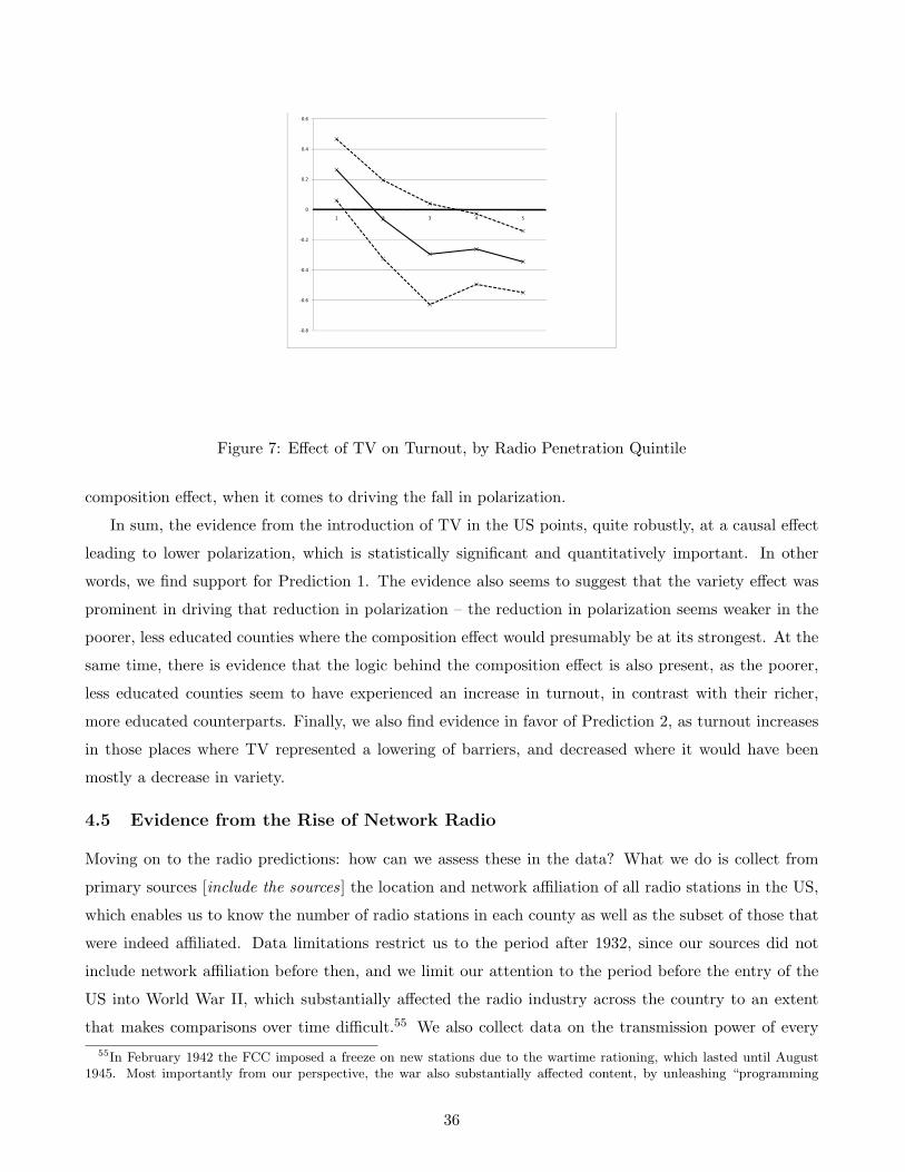
‐0.8

‐0.6

‐0.4

‐0.2

0

0.2

0.4

0.6

1 2 3 4 5

Figure 7: Effect of TV on Turnout, by Radio Penetration Quintile

composition effect, when it comes to driving the fall in polarization.

In sum, the evidence from the introduction of TV in the US points, quite robustly, at a causal effect

leading to lower polarization, which is statistically significant and quantitatively important. In other

words, we find support for Prediction 1. The evidence also seems to suggest that the variety effect was

prominent in driving that reduction in polarization – the reduction in polarization seems weaker in the

poorer, less educated counties where the composition effect would presumably be at its strongest. At the

same time, there is evidence that the logic behind the composition effect is also present, as the poorer,

less educated counties seem to have experienced an increase in turnout, in contrast with their richer,

more educated counterparts. Finally, we also find evidence in favor of Prediction 2, as turnout increases

in those places where TV represented a lowering of barriers, and decreased where it would have been

mostly a decrease in variety.

4.5 Evidence from the Rise of Network Radio

Moving on to the radio predictions: how can we assess these in the data? What we do is collect from

primary sources [include the sources] the location and network affiliation of all radio stations in the US,

which enables us to know the number of radio stations in each county as well as the subset of those that

were indeed affiliated. Data limitations restrict us to the period after 1932, since our sources did not

include network affiliation before then, and we limit our attention to the period before the entry of the

US into World War II, which substantially affected the radio industry across the country to an extent

that makes comparisons over time difficult.55 We also collect data on the transmission power of every55In February 1942 the FCC imposed a freeze on new stations due to the wartime rationing, which lasted until August

1945. Most importantly from our perspective, the war also substantially affected content, by unleashing “programming

36

 

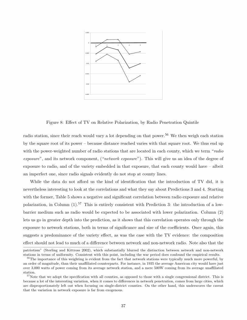
‐0.025

‐0.02

‐0.015

‐0.01

‐0.005

0

0.005

1 2 3 4 5

Figure 8: Effect of TV on Relative Polarization, by Radio Penetration Quintile

radio station, since their reach would vary a lot depending on that power.56 We then weigh each station

by the square root of its power – because distance reached varies with that square root. We thus end up

with the power-weighted number of radio stations that are located in each county, which we term “radio

exposure”, and its network component, (“network exposure”). This will give us an idea of the degree of

exposure to radio, and of the variety embedded in that exposure, that each county would have – albeit

an imperfect one, since radio signals evidently do not stop at county lines.

While the data do not afford us the kind of identification that the introduction of TV did, it is

nevertheless interesting to look at the correlations and what they say about Predictions 3 and 4. Starting

with the former, Table 5 shows a negative and significant correlation between radio exposure and relative

polarization, in Column (1).57 This is entirely consistent with Prediction 3: the introduction of a low-

barrier medium such as radio would be expected to be associated with lower polarization. Column (2)

lets us go in greater depth into the prediction, as it shows that this correlation operates only through the

exposure to network stations, both in terms of significance and size of the coefficients. Once again, this

suggests a predominance of the variety effect, as was the case with the TV evidence: the composition

effect should not lead to much of a difference between network and non-network radio. Note also that the

patriotism” (Sterling and Kittross 2002), which substantially blurred the distinction between network and non-networkstations in terms of uniformity. Consistent with this point, including the war period does confound the empirical results.

56The importance of this weighting is evident from the fact that network stations were typically much more powerful, byan order of magnitude, than their unaffiliated counterparts. For instance, in 1935 the average American city would have justover 3,000 watts of power coming from its average network station, and a mere 500W coming from its average unaffiliatedstation.

57Note that we adopt the specification with all counties, as opposed to those with a single congressional district. This isbecause a lot of the interesting variation, when it comes to differences in network penetration, comes from large cities, whichare disproportionately left out when focusing on single-district counties. On the other hand, this underscores the caveatthat the variation in network exposure is far from exogenous.

37

Table 5. Effects of Radio Exposure on Political Outcomes, 1932-41 (All counties)

(1) (2) (3) (4) (5) (6) (7) (8)

relative relative absolute absolute lopsided lopsided turnout turnout

Radio Exposure -0.00014** -0.00010** -0.0061 0.0055*

[0.00006] [0.00005] [0.0040] [0.0030]

Network -0.00019*** -0.00013*** -0.0015 0.0055*

[0.00006] [0.00005] [0.0031] [0.0032]

Non-Network -0.00001 -0.00003 -0.0201 0.0059

[0.00016] [0.00015] [0.0127] [0.0051]

Observations 10623 10623 10623 10623 10665 10665 10665 10665

# of counties 2521 2521 2521 2521 2574 2574 2574 2574

R-squared 0.22 0.22 0.23 0.23 0.08 0.08 0.48 0.48 Robust standard errors in brackets, clustered by county. All regressions include county fixed effects and region-year dummies. Controls are: log population, density, percent urban, percent nonwhite.

*** p<.01, ** p<.05, * p<.1

same pattern is true when it comes to absolute polarization, as shown in Columns (3) and (4), although

the results are undistinguished when it comes to the measure of lopsidedness of elections.

When it comes to Prediction 4, on turnout, the results are less clear. Columns (7) and (8) show

some evidence of a positive correlation between exposure to radio and turnout, in line with the results

in Stromberg (2004). In this case, it seems that there is no particular distinction between affiliated and

unaffiliated stations. The information / motivation impact of the introduction of the new medium seems

to have dominated any possible negative impact on turnout that lower polarization might have induced.

In sum, and with the caveat that no causality claim is warranted from this evidence, the results

are consistent with the idea that (network) radio had a similar depolarizing effect to that which TV

would also have later on. Also in line with the TV results, there is also evidence that such depolarizing

effect would have been attributable, to a substantial extent, to the variety effect predicted by the theory.

38

Broadly speaking, we have good reason to believe that the evolution of media technologies between the

1930s and 1950s had a significant role in the drop in polarization observed over that period.

5 Concluding Remarks

This paper has developed a framework that allows us to understand the impact of changes in media

technology on the distribution of political preferences, and thus on equilibrium levels of polarization.

Building on a simple model of how media exposure affects individual ideological positions, married to a

model of how these affect politicians’ behavior through electoral competition, we identify two different

channels through which that impact takes place: the composition effect and the variety effect. The former

stems from the fact that exposure to media affects the levels of information and political motivation, and

hence turnout decisions. Because those levels, in turn, are generally different for ideologically moderate

individuals than for those who are ideologically extreme, this affects equilibrium polarization. The latter

effect arises from the influence that media technologies exert over individuals’ ideological views. As a

result, changes in the scope of ideological variety supplied by the media will also affect the distribution

of those views, and hence polarization.

In addition to that, we provide empirical evidence, gauged from the episodes of introduction of TV

and network radio in the US, that supports the prediction that these new technologies – since they implied

substantial decreases in variety and increases in accessibility – would engender reductions in polarization.

This suggests that the substantial reduction in polarization that occurred in the US around the mid-20th

century was helped by the changes in media environment, as had been suggested for instance by Prior

(2007). The evidence also enables us to try to disentangle the two effects predicted by the theory: it

seems that the variety effect, namely the direct impact of the media on individuals’ ideological views,

was at the heart of the changes.

An important advantage of our theoretical framework is that it can be broadly applied, presumably

to any changes in media technology, which we codify simply according to accessibility and variety. For

instance, one could use it to think about the effects of recent changes, such as the diffusion of cable TV

or the internet or even talk radio, which have all been accused of increasing polarization (Prior 2007,

Bishop 2008, Sunstein 2009). In particular, our evidence that the variety effect was more important

than the composition effect in explaining the effects of media technologies on polarization, for the case

of radio and broadcast TV in the US, does not imply that this would be the case in other contexts. Our

theory also suggests, and the data support, that the same technology could have very different effects

depending on the media substrate into which it is introduced. This could be especially interesting in

the context of comparing different countries: the introduction of the internet could have a very different

impact when it takes place in a context dominated by a high-variety medium (say, cable TV), as is

probably a good description for the US, than when the backdrop is state-owned broadcast TV. Such

39

cross-country comparisons are also particularly interesting in that our theory suggests that differences

in political institutions will affect the effects of media – it would be worthwhile to empirically check for

the predictions under a proportional representation system. We believe these are all exciting topics for

future research.

By the same token, future research may also focus on exploring the implications of our model of how

media affects preferences, and vice-versa. We have proposed a theory of the individuals’ demand for

ideological variety, and it seems natural to extend the analysis to incorporate the supply side and the

equilibrium provision of variety. In the context of our model, this would involve endogenizing market

variety (M) and the “budget” allocated to media consumption – which would include the extensive

margin of choosing not to consume at all. This would connect naturally with the literature on media

slant, as in Mullainathan and Shleifer (2005), towards a dynamic theory of how ideology evolves, tied to

issues such as technological features and regulation (switching costs, different sources of revenue such as

subscription vs advertising, etc.). These are some of the avenues that we intend to pursue.

40

6 References

Aldrich, John H. (1993). “Rational Choice and Turnout.” American Journal of Political Science 37:246-278.

Alesina, Alberto and Howard Rosenthal (1995). Partisan Politics, Divided Government, and the Econ-omy. Cambridge, UK: Cambridge University Press.

APSA Committee on Political Parties (1950). “Toward a More Responsible Two-Party System.” Amer-ican Political Science Review 44: supplement.

Austen-Smith, David and Jeffrey S. Banks (2005). Positive Political Theory I: Collective Preferences.Ann Arbor, MI: University of Michigan Press.

Bagnoli, Mark and Ted Bergstrom (2005). “Log-Concave Probability and Its Applications.” EconomicTheory 26(2): 445-469.

Benjamin, Louise M. (2001). Freedom of the Air and the Public Interest: First Amendment Rights inBroadcasting to 1935. Carbondale, IL: Southern Illinois University Press.

Binder, Sarah A. (1999). “The Dynamics of Legislative Gridlock, 1947-1996.” American PoliticalScience Review 93(3): 519-533.

Bishop, Bill (2008). The Big Sort: Why the Clustering of Like-Minded America Is Tearing Us Apart.New York: Houghton Mifflin Harcourt.

Cohen, Lizbeth (1990). Making a New Deal: Industrial Workers in Chicago, 1919-1939. Cambridge,UK: Cambridge University Press.

Converse, Philip E. (1962). “Information Flow and the Stability of Partisan Attitudes.” Public OpinionQuarterly 26(4): 578-599.

Coughlin, Peter J. (1992). Probabilistic Voting Theory. Cambridge, UK: Cambridge University Press.

Della Vigna, Stefano and Matthew A. Gentzkow (2009). “Persuasion: Empirical Evidence.” Universityof Chicago mimeo.

Della Vigna, Stefano and Ethan Kaplan (2007). “The Fox News Effect: Media Bias and Voting.”Quarterly Journal of Economics 122(3): 1187-1234.

Dionne, E.J. (2004). Why Americans Hate Politics. New York: Simon and Schuster.

Downs, Anthony (1957). An Economic Theory of Democracy. New York: Harper.

Duggan, John (2000). “Equilibrium Equivalence under Expected Plurality and Probability of WinningMaximization.” University of Rochester mimeo.

Durante, Ruben and Brian Knight (2009). “Partisan Control, Media Bias, and Viewer Responses:Evidence from Berlusconi’s Italy.” Brown University mimeo.

Ellner, Steve and Daniel Hellinger (eds.) (2004). Venezuelan Politics in the Chavez Era: Class, Polar-ization, and Conflict. Boulder, CO: Lynne Rienner.

Fiorina, Morris P., with Samuel J. Abrams and Jeremy C. Pope (2006). Culture War? The Myth ofPolarized America. New York: Pearson Longman.

Gentzkow, Matthew A. (2006). “Television and Voter Turnout.” Quarterly Journal of Economics121(3): 931-972.

Gentzkow, Matthew A. and Jesse M. Shapiro (2004). “Media, Education and Anti-Americanism in theMuslim World.” Journal of Economic Perspectives 18(3): 117-133.

41

Gentzkow, Matthew A. and Jesse M. Shapiro (2008). “Media Bias and Reputation.” Journal of PoliticalEconomy 114(2): 280-316.

Gentzkow, Matthew A., Jesse M. Shapiro, and Michael Sinkinson (2009). “The Effect of NewspaperEntry and Exit on Electoral Politics.” University of Chicago mimeo.

Gerber, Alan, Dean Karlan, and Daniel Bergan (2009). “Does the Media Matter? A Field Experi-ment Measuring the Effect of Newspapers on Voting Behavior and Political Opinions.” AmericanEconomic Journal: Applied Economics 1(2): 35-52.

Gerbner, George, Larry Gross, Michael Morgan, and Nancy Signorielli (1980). “The ‘Mainstreaming’of America: Violence Profile No. 11.” Journal of Communication 30(3): 10-29.

Glaeser, Edward L., Giacomo A.M. Ponzetto, and Jesse M. Shapiro (2006). “Strategic Extremism: WhyRepublicans and Democrats Divide on Religious Values.” Quarterly Journal of Economics 120(4):1283-1330.

Groseclose, Tim and Jeffrey Milyo (2005). “A Measure of Media Bias.” Quarterly Journal of Economics120(4): 1191-1237.

Hamilton, James T. (2004). All the News That’s Fit to Sell: How the Market Transforms Informationinto News. Princeton, NJ: Princeton University Press.

Jensen, Robert and Emily Oster (2009). “The Power of TV: Cable Television and Women’s Status inIndia.” Quarterly Journal of Economics 124(3): 1057-1094.

Jones, David R. (2001). “Party Polarization and Legislative Gridlock.” Political Research Quarterly54(1): 125-141.

Krugman, Paul R. (2004). The Great Unraveling: Losing Our Way in the New Century. New York:W.W. Norton & Co.

La Ferrara, Eliana, Alberto Chong, and Suzanne Duryea (2008). “Soap Operas and Fertility: Evidencefrom Brazil.” IGIER Bocconi mimeo.

Ledyard, John O. (1984). “The Pure Theory of Large Two-Candidate Elections.” Public Choice 44(1):7-41.

McCarty, Nolan (2007). “The Policy Effects of Political Polarization.” In: Paul Pierson and ThedaSkocpol (eds.), The Transformation of American Politics: Activist Government and the Rise ofConservatism. Princeton, NJ: Princeton University Press.

McCarty, Nolan, Keith T. Poole and Howard Rosenthal (undated). “Political Polarization and IncomeInequality.” Princeton University mimeo, available at: http://www.princeton.edu/∼nmccarty/ineqpold.pdf

McCarty, Nolan, Keith T. Poole and Howard Rosenthal (2006) Polarized America: The Dance of Ide-ology and Unequal Riches. Cambridge, MA: MIT Press.

Mullainathan, Sendhil and Andrei Shleifer (2005). “The Market for News.” American Economic Review95: 1031-1053.

Murphy, Kevin M. and Andrei Shleifer (2004). “Persuasion in Politics.” American Economic Review94(2): 435-439.

Pew Research Center for the People and the Press (2008). “Audience Segments in a Changing NewsEnvironment: Key News Audiences Now Blend Online and Traditional Sources (April 2008 MediaSurvey).” Available at: http://people-press.org/dataarchive/#2008.

Pfau, Michael, J. Brian Houston, and Shane M. Semmler (2007). Mediating the Vote: The ChangingMedia Landscape in U.S. Presidential Campaigns. Lanham, MD: Rowman & Littlefield.

42

Prior, Markus (2007). Post-Broadcast Democracy: How Media Choice Increases Inequality in PoliticalInvolvement and Polarizes Elections. Cambridge, UK: Cambridge University Press.

Riker, William and Peter Ordeshook (1968). “A Theory of the Calculus of Voting.” American PoliticalScience Review 62: 25-42.

Sinclair, Barbara (2006). Party Wars: Polarization and the Politics of National Policy Making. Nor-man, OK: University of Oklahoma Press.

Stromberg, David (2004). “Radio’s Impact on Public Spending.” Quarterly Journal of Economics119(1): 189-221.

Sterling, Christopher H. and John Michael Kittross (2002). Stay Tuned: A History of American Broad-casting, 3rd ed. Mahwah, NJ: LEA.

Sunstein, Cass R. (2009). Going to Extremes: How Like Minds Unite and Divide. Oxford, UK: OxfordUniversity Press.

Webster, James G. (1986). “Audience Behavior in the New Media Environment.” Journal of Commu-nication 36(3): 77-91.

43

A Proofs

A.1 Variety and Ideology

Proof of Proposition 1.The demand τ∗(z, φ,M) for varieties of a consumer with ex-ante ideology z ∈ X in a market with

variety M solvesmax

τ∈∆(M)W (z, τ) ≡ λ(|z −H(z, τ)|)− φ(τ).

The result is established by characterizing the solution to this problem.If z /∈ Σ(M) then, regardless of φ(τ), the optimal choice is τ∗(z, φ,M) = δm∗(z). Indeed, this choice

achieves the smallest possible dissonance |z −H(z, τ)| across consumption plans τ ∈ ∆(M) and φ(τ) ≥φ(δm∗(z)) = 0.

If z ∈ Σ(M) there are two cases. Either the optimal consumption involves switching or not. In thefirst case, assumption (A1) ensures that τ∗(z, φ,M) can be chosen so that H(z, τ∗(z, φ,M)) = z, i.e.,zero dissonance. Without loss of generality, let λ(0) = 0. In general, unless z = m for m ∈M , the valueof a plan that leaves a consumer’s ideology unchanged is λ(0)−φ = −φ (if z = m no switching is requiredto achieve zero dissonance). The best plan without switching is δm∗(z). It follows that the optimal planis switching iff

φ ≤ λ(|z −H(z, δm∗(z))|) (4)

Since |z −H(z, δm∗(z))| is an increasing function of |z −m∗(z)|, from (4) it follows that there existsK(·) is an increasing function, such that if φ ≤ K(|z −m∗(z)|) then τ∗(z, φ,M) can be chosen so thatH(z, τ∗(z, φ,M)) = z. Instead, if φ ≥ K(|z −m∗(z)|) then τ∗(z, φ,M) = δm∗(z). This, combined withour observation for z /∈ Σ(M) establishes (i) and (ii).

To show (iii), let Σ(M) = [σ−, σ+]. Suppose that z ≤ σ− so that m∗(z) = σ−. From (ii), the ex-postideology is given by x(z) = H(z, δσ−) and, by assumption (A1), H(·, ·) is increasing in its first argumentfrom which x(z) is increasing for all z ≤ σ−. The case z ≥ σ+ is analogous. If M = Σ(M) = {m}so that σ− = σ+, we are done. Suppose instead that σ− < σ+ and consider z ∈ Σ(M). Recall thatM = {m1, ...,mn} with σ− = m1 and σ+ = mn, and Σ(M) can be partitioned into subintervals of theform Σi = [mi,mi+1], where each of the extremes correspond to adjacent varieties offered in the market.Note that if z = mi then τ∗(z, φ,M) = mi and H(z, τ∗(z, φ,M)) = z. To conclude the proof it suffices toshow that H(z, τ∗(z, φ,M)) is increasing in z within each Σi. Observe that the largest distance betweena point in the interval and one of the extremes is the midpoint zmidi = (mi + mi+1)/2 and the distanceto either mi or mi+1 is (mi+1 −mi)/2. From (i) and (ii), we conclude that there exist m−i ,m

+i ∈ Σ(M)

with m−i < zmidi < m+i such that (i) if z ∈ [mi,m

−i ) ∪ (mi,m

+i ] then φ > K

(|z −H(z, δm∗(z)

)|),

τ∗(z, φ,M) = δmi for z ∈ [mi,m−i ) and τ∗(z, φ,M) = δmi+1 for z ∈ (mi,m

+i ]; (ii) if z ∈ [m−i ,m

+i ] then

φ ≤ K (|z −H(z, δmi) |) and τ∗(z, φ,M) is such that H(z, τ∗(z, φ,M)) = z. Clearly, H(z, τ∗(z, φ,M)) isstrictly increasing in each of the intervals [mi,m

−i ), [m−i ,m

+i ], and (mi,m

+i ]. Furthermore, H(m−i , δmi) <

m−i and H(m+i , δmi+1) < m+

i . It follows that H(z, τ∗(z, φ,M)) is increasing on Σi, and thus, on Σ asdesired. �

Proof of Proposition 2.Suppose that φ = 0. For each balanced market variety M ⊂ X and Σ(M) = [σ−, σ+] is the variety

span. If M is balanced then σ− + k = σ+ − k = x. Given z ∈ X let RM (z) ≡ H(z, τ∗(z, φ,M)) be thecorresponding ex-post ideology and recall that GM (x) = G0(RM (x)). Invoking Proposition 1(i),

RM (x) =

H(x, δσ−) if x < σ−

x if x ∈ [σ−, σ+]H(x, δσ+) if x > σ+.

To establish the result we consider an infinitesimal increase in σ− and one in σ+. (Recall that forφ = 0 a balanced decrease in variety amount to increasing σ− and decreasing σ+ by the same amount.Assumption (A1)(H3) implies that H(x, δσ) < H(x, δσ′) if σ′ > σ. It follows that ∂H(x,δσ)

∂σ > 0, fromwhich ∂GM (x)

∂σ− = g0(RM (x))∂H(x,δσ)∂σ > 0. �

44

We conclude with an intuitive lemma that follows from proposition 1 and is used in the proof ofproposition 3. The proof is omitted.

Lemma 6 Suppose that φ = 0 and fix a market with variety M . If M ′ is a balanced decrease in varietywith respect to M then gM ′(x) ≥ gM (x) with strict inequality if M ′ = {x}.

In words, since a reduction in variety leads to a compression of the distribution, it cannot reduce themass of voters with the median ideology.

A.2 Political Equilibrium: Analysis

We introduce some notation and terminology used in the proofs. Write ε for the set of parameters of themodel. Let

y(z, ε) = x− c

2zand

Q(z, ε) = pg(x) + (1− p)g(y(z, ε))− 12ρ(x0R − x0L − z)

We say x∗ is an interior equilibrium of the electoral game if xL0 < x∗L < x∗R < x0R.

Lemma 7 If x∗ is an interior equilibrium of the electoral game then ∆x∗ = x∗R−x∗L solves Q(∆x∗, ε) = 0.

Proof. Each candidate’s policy must satisfy a first order condition (FOC). For L the FOC is

∂WL

∂xL(x∗L, x

∗R)− ρ(x∗L − xL0) = 0.

Observe that under assumption (A4), ∂WL∂xL

= ∂VL∂xL− ∂VR

∂xL, where

∂VL∂xL

=12pg(x1/2) + (1− p)g(yL)

∂yL∂xL

and∂VR∂xL

= −12

[pg(x1/2) + (1− p)g(yR)

∂yR∂xL

].

If G has unbounded support, yL(x) = x1/2 − c2(xR−xL) and yR(x) = x1/2 + c

2(xR−xL) , from which ∂yL∂xL

=12

(1− c

2(xR−xL)2

)and ∂yL

∂xL= 1

2

(1 + c

2(xR−xL)2

). Now, for a symmetric equilibrium, we have that x∗1/2 =

x, x∗L − xL0 = 12(x0R − x0L −∆x∗) and, since g is symmetric with respect to x, g(yR(x∗)) = g(yR(x∗)).

Combining the previous, the FOC at an equilibrium point is

pg(x) + (1− p)g(y(∆x∗, ε))− 12ρ(x0R − x0L −∆x∗) = 0, (5)

or Q(∆x∗, ε) = 0.

Lemma 8 Q(∆x∗, ε) = 0 has a solution 0 < ∆x∗ < xR0 − xL0. Furthermore, the largest and smallestsolutions of Q(∆x∗; ε) = 0 in [0, xR0 − xL0] satisfy ∂Q

∂z (∆x∗, ε) > 0. These two solutions are equilibria ofthe electoral competition game.

Proof. Observe that Q(x0R − x0L, ε) = pg(x) + (1− p)g(y(∆x∗, ε)) ≥ pg(x) > 0 for all ε. On the otherhand, y(0, ε) = −∞, so that g(y(∆x∗, ε)) = 0. It follows that Q(0, ε) = pg(x) − 1

2ρ(x0R − x0L − ∆x∗).From assumption (P6), Q(0, ε) < 0. Since Q(0, ε) < 0, Q(x0R−x0L, ε) > 0, and Q is continuous in its firstargument, we conclude by the intermediate value theorem that Q(z∗; ε) = 0 for some z∗ ∈ (0, xR0−xL0).

Since Q(0, ε) < 0, for the smallest solution Q(z∗; ε) crosses the zero from below. Similarly, sinceQ(x0R − x0L, ε) > 0, the same is true for the largest solution. It follows that ∂Q

∂z (∆x∗, ε) > 0 where ∆x∗is either the largest or smallest solution of Q(∆x∗, ε) = 0.

Finally, observe that Q(∆x∗, ε) = 0 follows from the candidates’ necessary FOC. For the case of thesmallest and largest solution it can be shown that this FOC is associated with the unique best responsefor each candidate.

45

Lemma 9 Given the c.d.f. G and the corresponding p.d.f.g let rG(x, y) = g(x)−g(y)G(x)−G(y) . If g is log-concave

then rG(x, y) ≤ g′(y)g(y) for all y ≤ x.

Proof. rG(x, y) ≤ g′(y)g(y) for all y ≤ x⇔ S(x, y) ≡ (G(x)−G(y)) g′(y)− g(y) (g(x)− g(y)) ≥ 0 for all y ≤

x. Note that S(y, y) = 0. Differentiating S(x, y) with respect to x we get Sx(x, y) = g(x)g′(y)−g(y)g′(x).This is strictly positive for x ≥ y as long as g is log-concave.

Proof of Proposition 3(i) From lemma 7, an interior equilibrium satisfies Q(∆x∗, ε) = 0. It follows that ∂∆x∗

∂p = −∂Q∂p /

∂Q∂z . For

the highest and lowest equilibrium ∂Q∂z > 0 (Lemma 8) Hence, if ∂Q

∂p < 0. then ∂∆x∗

∂p > 0. Now,

∂Q

∂p= g(x)− g(y(∆x∗, ε)) > 0.

Similarly,∂Q

∂c= −(1− p)g′(y(∆x∗, ε))

1∆x∗2

,

which is less than zero if g is increasing at y(∆x∗, ε).(ii) As argued in the main text, letting ∆G = G(yR(x∗))−G(yL(x∗)) and y′ = ∂y(∆x∗,ε)

∂z = c2∆x∗2 > 0 for

short,∂V ∗

∂p= ∆G+ 2(1− p)g(y(∆x∗, ε))y′

∂∆x∗

∂p

and, from (i), letting ∆g = g(x)− g(y(∆x∗, ε)),

∂∆x∗

∂p= −∂Q

∂p/∂Q

∂z= − ∆g

(1− p)g′(y(∆x∗, ε))y′ + 12ρ.

Thus, ∂V ∗

∂p > 0 iff

⇔(

(1− p)g′(y(∆x∗, ε))y′ +12ρ

)∆G− 2(1− p)g(y(∆x∗, ε))y′∆g ≥ 0

⇔ (1− p)y′[g′(y(∆x∗, ε))g(y(∆x∗, ε))

− 2∆g∆G

]+

12ρ ≥ 0

⇔ (1− p)y′[g′(y(∆x∗, ε))g(y(∆x∗, ε))

− rG(x, y(∆x∗, ε))]

+12ρ ≥ 0

where rG(x, y) = g(x)−g(y)G(x)−G(y) and we used G(yR(x∗)) − G(yL(x∗)) = 2 (G(x)−G(y)). The latter follows

from symmetry. By Lemma 9, g′(y)g(y) − rG(x, y) ≥ 0 and the expression above is positive as desired. �

Proof of Proposition 4.Let M be the market’s ideological variety and GM be the associated distribution of citizens’ ideologies.If M is balanced with respect to x, the market variety span can be expressed as Σ(M) = [x−k, x+k] forsome k > 0. The variety span is entirely determined by k, with larger k associated with more variety, wewrite M = Mk. If Mk′ is a balanced decrease in variety with respect to Mk then k′ < k. To establish (i)we show that an decrease in k is associated with an decrease of the equilibrium polarization level ∆x∗(k)for the (smallest and largest equilibrium) or, equivalently, ∆x∗(k) is increasing in k.(i) From Lemma 7 we have that the equilibrium level of polarization ∆x∗(k) satisfies Q(∆x∗(k), ε) = 0,where

Q(z, ε) = pgMk(x) + (1− p)gMk

(y(z, ε))− 12ρ(x0R − x0L − z)

46

Since ∂Q∂z > 0 for the smallest and largest equilibrium, ∆x∗(k) increases with k if Q(z, ε) deceases with k.

From Lemma 6 gMk(x) ≤ gMk′ (x) if k′ < k. The corresponding change in gMk

(y(z, ε)) has an ambiguoussign. However, for p large enough the conclusion follows.(ii) As illustrated in the main text the direct effect of the compression induced by the decrease in marketvariety is to reduce turnout as, all else equal, those who do not turnout are precisely the moderateswith low motivation. The indirect effect derives from the change in turnout associated to the change inplatforms. From (i), this movement promotes moderation by the candidates which, in turn, is associatedwith lower turnout by moderate citizens with low motivation. �

A.2.1 Proportional Representation

Under Assumption (A4’) we can introduce definitions similar to the ones used for the analysis of electoralcompetition under Assumption (A4) to obtain the comparative statics we are interested in. As before letε be the parameters of the model and define γ = g(x)

|x0R−x0L|ρ . The analogues of y(·, ·) and Q(·, ·) definedabove are given by

y(z, ε) = x− c

2|x0R − x0L|1z

and

Γ(z; ε) = γ

[1 + 1−p

p

g(y(z, ε))g(x)

]− (1− z)

[1 + 1−p

p

G(y(z, ε))G(x)

].

The proofs of the following two Lemmas parallel those of Lemmas 7 and 8, and are thus omitted.They are available upon request.

Lemma 10 If x∗ is an interior equilibrium of the electoral game then ∆∗ = x∗R−x∗L

xR0−xL0solves Γ(∆∗; ε) = 0.

Lemma 11 Γ(∆∗; ε) = 0 has a solution ∆∗ ∈ (0, 1). Furthermore, the largest and smallest solution ofΓ(∆∗; ε) = 0 satisfy ∂Γ

∂z (∆∗; ε) > 0. These two solutions correspond to equilibria of the electoral competitiongame.

Proof of Proposition 5.(i) From lemma 10, an interior equilibrium satisfies Γ(∆∗; ε) = 0. It follows that ∂∆∗

∂p = −∂Γ∂p /

∂Γ∂z . For

the highest and lowest equilibrium ∂Γ∂z > 0 (Lemma 11.) Hence, if ∂Γ

∂p < 0. then ∂∆∗

∂p > 0. Now,

∂Γ∂p

=1p2

(−γ g(y(∆∗, ε))

g(x)+ (1−∆∗)

G(y(∆∗, ε))G(x)

).

From Γ(∆∗; ε) = 0 we have that γ1−∆∗ =

1+1−pp

G(y(∆∗,ε))G(x)

1+1−pp

g(y(∆∗,ε))g(x)

so the above expression becomes

∂Γ∂p

=(1−∆∗)

(1 + 1−p

pG(y(∆∗,ε))

G(x)

)p2

(−r(g(y(∆∗, ε))

g(x)

)+ r

(G(y(∆∗, ε))

G(x)

))where r(z) ≡ z

1+1−pp z

. Our hypothesis that on the log-concavity of G implies that gG is decreasing. Since

y(∆∗, ε) < x, we have that g(y(∆∗,ε))g(x) > G(y(∆∗,ε))

G(x) . Since r(·) is increasing we conclude that ∂Γ∂p < 0.

(ii) As argued in the main text, the direct effect of an increase in p on turnout is positive. In addition,from (i) we have that the indirect effect on turnout (which arises from the change in platforms) as anincrease in polarization ∆∗ without changing x1/2 = x leads to higher turnout from citizens with lowpolitical motivation. �

47

B Switching costs and ideological compression

Let us explore in greater depth the model of media and ideology in Section 2.3, for a general level ofswitching costs, φ. Note first that, regardless of φ, if M = X then GM,φ = G0, as a result of proposition1. In other words, if all ideologies are available, the distribution will not be affected by the media, asindividuals can always find a perfect match for their initial view. (If φ ≡ 0 this equality remains ifthe much weaker condition Σ(M) = X holds, as in this case individuals can always combine existingmedia to construct an exact match.) By the same token, if there is minimal variety (M = {m}), thenGM,φ is independent of φ as well. Furthermore, if m = x where x is the median of G0 then GM,φ is acompression of G0. We can thus see that, in going from one extreme of complete variety to the otherof minimal variety, our intuition is confirmed regardless of φ. However, the following example illustrateshow monotonicity is not guaranteed in general, as depending on φ a relatively low supply of ideologicalvariety can either compress or disperse the ideologies of citizens.

Example 2 Suppose that X = [−1, 1] and assume the market has two ideological varieties, m1 = −1/2and m2 = 1/2, i.e., M = {−1/2, 1/2}. This implies that Σ(M) = [−1/2, 1/2]. The distribution of priorideologies G0 is a symmetric triangle distribution with support X, it’s median is x = 0. For concretenesswe consider the linear influence function given by (1).

For φ = 0, from proposition 1 (i) and (1), we have that the support of the new distribution becomes[−1

2 − a12 ,

12 + a1

2

]and

RM,φ(x) =

x−(1−a)(− 1

2)

a if x ∈[−1

2 − a12 ,−

12

)x if x ∈ [−1/2, 1/2]

x−(1−a)( 12

)

a if x ∈(

12 ,

12 + a1

2

].

Using this and (2) it’s easy to verify that the distribution GM,φ is a compression of G0.Assuming φ is large enough so that 1(ii) holds for all ideologies, we have that the support of the new

distribution is the union of the intervals[−1

2 − a12 ,−(1− a)1

2

]and

[(1− a)1

2 ,12 + a1

2

], and

RM,φ(x) =

{x−(1−a)(− 1

2)

a if x ∈[−1

2 − a12 ,−(1− a)1

2

]x−(1−a)( 1

2)

a if x ∈[(1− a)1

2 ,12 + a1

2

].

In contrast to the case φ = 0, GM,φ is a dispersion of G0.

The example suggests that if a society or group of consumers is initially deprived from media accessand then gains access to a relatively low-variety media environment, their preferences may become moreor less concentrated, depending on the cost φ. For instance, the introduction of a duopoly of newspaperswith different editorial lines could be associated with a dispersion if conscientious readers are a negligiblefraction (say, due to subscription pricing or spatial segregation in the distribution), or with a compressionif the opposite holds. Note also that the example suggests that, with negligible switching costs, the modeldoes exhibit the monotonicity property, which does not apply to the model with high costs.

48

Table A1. Effect of Ideological Extremism on Likelihood of Watching Both Fox News and MSNBC

Probit regressions, robust standard errors in brackets. All regressions include as controls the response to the question on attention to hard news (hardnews) and individual ideology (ideo). The measure of extremism is defined as the absolute value of (ideo – 2), since 2 is the value that corresponds to “moderate”. Demographic controls are: sex, marital status and race dummies, age, education, income. The sample includes only individuals who answered “Regularly” or “Sometimes” to the question of how often she watches Fox News or CNN or MSNBC, and excludes individuals who did not answer one of the demographic questions. *** p<.01, ** p<.05, * p<.1 Source: Pew Research Center for the People and the Press, April 2008 Media Survey: Audience Segments in a Changing News Environment: Key News Audiences Now Blend Online and Traditional Sources (Aug 17, 2008).

 

  (1) (2) (3)

       

Extremism  ‐0.1112[0.0803] 

‐0.1402*[0.0813] 

‐0.1534*[0.0859] 

Demographic Controls  Yes Yes

State FEs  Yes

 

Observations  617 616 603

R‐Squared  0.003 0.043 0.095

49