mechatronic modeling and control of a doubly-fed … issue 6/version-2...mechatronic modeling and...

IOSR Journal of Electrical and Electronics Engineering (IOSR-JEEE)

e-ISSN: 2278-1676,p-ISSN: 2320-3331, Volume 12, Issue 6 Ver. II (Nov. – Dec. 2017), PP 31-44

www.iosrjournals.org

DOI: 10.9790/1676-1206023144 www.iosrjournals.org 31 | Page

Mechatronic Modeling And Control of A Doubly-Fed Wind

Turbine Induction Generator Using The Bond Graph Approach

Zakaria Khaouch1,Mustapha Zekraoui

1,Mustapha Adar

1,Nourreeddine

Kouider1,Mustapha Mabrouki

1

1Industrial Engineering Laboratory, Faculty of Science and Technology, Sultan Moulay Slimane University,

Beni Mellal, Morocco.

Corresponding Author: Zakaria Khaouch1

Abstract: This paper describes a Bond Graph modeling and control of a doubly-fed induction generator driven

by a wind turbine and running at variable speed. This type of operation will retrieve at any time the maximum

power regardless of the wind speed. Initially, the Bond Graph tool is used to model the doubly-fed induction

generator, the real dynamic behavior of this system is taken into account, consequently, final load simulation is

more realistic offering benefits and reliable system performance. Thereafter, we will discuss the theoretical

development related to the control of the doubly-fed wind turbine generator using the concept of bicausality of

Bond Graph based on the wind turbine model presented in a previous work.

Keywords: Bicausality, Bond graph, Doubly fed induction generator, Invers model, Wind turbine. ------------------------------------------------------------------------------------------------------------------------------------ ---

Date of Submission: 07-11-2017 Date of acceptance: 30-11-2017

----------------------------------------------------------------------------------------------------------------------------- ----------

I. Introduction Since ancient times, wind has been exploited in different ways, mainly for grain milling and water

pumping. A wind turbine is a device that extracts kinetic energy from the wind and converts it into electrical

energy. Wind turbines can be classified into two categories [1], namely: Fixed Speed Wind Turbine (FSWT)

and Variable-Speed Wind Turbine (VSWT). Compared to VSWT, FSWT are easy to construct and operate, but

VSWT have the advantages of improved energy capture, reduction in transient load and better power

conditioning [2].Nowadays, VSWT are increasingly used in comparison with FSWT, and the Doubly-Fed

Induction Generator (DFIG) is the most variable speed machine commonly used in production units. The DFIG

offers the advantages of speed control with reduced cost and power losses [3, 4, 5].

Modeling and control of a DFIG has been addressed in several works, e.g. [6, 7, 8, 9]. In [6] a robust

fractional-order sliding mode (FOSM) controller is used, and [7] presents an intelligent proportional-integral

sliding mode control (iPISMC) for direct power control of variable speed-constant frequency wind turbine

system. A self-optimizing robust control scheme that can maximize the power generation for a variable speed

wind turbine with DFIG operated in Region 2 is proposed in [8]. A simplified model of the DFIG is presented in

[9]. In this paper, a different structure for the DFIG control, based on the Bond Graph methodology [10, 11] is

proposed.

Wind turbine is a complex mechatronic system, in which different technical areas are involved

(mechanics, aeronautics, electrical, among others). There is no doubt that a mechatronic approach is essential in

the field of wind turbine design [12]. This approach implies that mechanic, aerodynamic, electric subsystems

and eventually their control subsystem should be designed as an integrated system. This integration is important

for a more accurate evaluation of the extreme loads and the fatigue life, and this might reduce the failure rate in

the design stage. In [12] a detailed mechatronic model of the wind turbine is proposed using the Bond Graph

Approach. All parts of the wind turbine are modeled in detail, the real dynamic behavior of the system is taken

into account, and as a result, the final load simulation is more realistic offering benefits and reliable system

performance. This model is taken as a reference platform to simulate the behavior of the proposed model control

presented in this present paper. In order to analyze the system in the same reference frame, the Bond-Graph

methodology can represent the whole structure. This methodology features some properties that can be directly

applied to the model [11].A Bond Graph [10, 11] is a graphical representation of a physical dynamic system. It

is similar to the better known block diagram and signal-flow graph, with the major difference that the arcs in

bond graphs represent bi-directional exchange of physical energy, while those in block diagrams and signal-flow

graphs represent uni-directional flow of information. Also, bond graphs are multi-energy domain (e.g.

mechanical, electrical, hydraulic, etc) and domain neutral. This means that a Bond Graph can incorporate

multiple domains seamlessly.

Mechatronic Modeling And Control of A Doubly-Fed Wind Turbine Induction Generator..


The Bond Graph is composed of the ”bonds” which link together ”single port”, ”double port” and

”multi port” elements. Each bond represents the instantaneous flow of energy (dE(t)/dt) or power P(t). A pair of

variables called ”power variables” whose product is the instantaneous power of the bond denotes the flow of

energy in each bond. Each domain’s power variables are broken into two types: ”effort e(t)” and ”flow f(t)”.

Effort multiplied by flow produces power, thus the term power variables. Every domain has a pair of power

variables with corresponding effort and flow variables.

The main advantages of the Bond Graph tool for modeling purposes is summarized through few keywords,

which makes this approach quite specific and justifies its use in the paper [12]. These are the following:

1. Modeling: the Bond Graph is a unified representation language, which highlights explicitly the power

flows, makes possible the energetic study, makes simpler the models building for multi-disciplinary

systems, shows up explicitly the cause - to effect relations (causality) and leads to a systematic writing of

mathematical models (linear or nonlinear associated).

2. Identification: identification of unknown parameters, but knowledge of the associated physical phenomena

and mastering physical meaning of the obtained model.

3. Analysis: Putting to the fore the causality problems, and therefore the numerical problems and estimation

of the dynamic of the model and identification of the slow and fast variables.

4. Control: Design of control laws from simplified models.

5. Simulation: Specific software (20-Sim)

In this contribution, the Bond Graph is used to model the DFIG and the control law is obtained by

means of bicausality concept [13]. The paper is structured into 7 sections. Section 2 is a short description of

wind turbine configurations. Section 3, deals with the bond graph model of DFIG. The models of wind turbine is

presented in Section 4. The proposed control approach is described in Section 4 and the whole simulated system

in Section 6. The global conclusions of the conducted investigation are drawn in Section 7.

II. System Description From the generator point of view, a wind turbine has different configurations. They are essentially

determined by the feasible ways to act on the turbine. Fixed-speed, variable-speed, fixed-pitch and variable-

pitch are the most common ones. Since wind turbines work under different conditions, these operating modes

are usually combined to achieve the control objectives over the full range of operational wind speeds.

Accordingly, wind turbines can be classified into four categories, namely:

• Fixed-speed wind turbine with an induction generator.

• Variable-speed wind turbine with a cage-bar induction generator or synchronous generator.

• Variable-speed wind turbine with multiple-pole synchronous generator.

• Variable-speed wind turbine with doubly-fed induction generator.

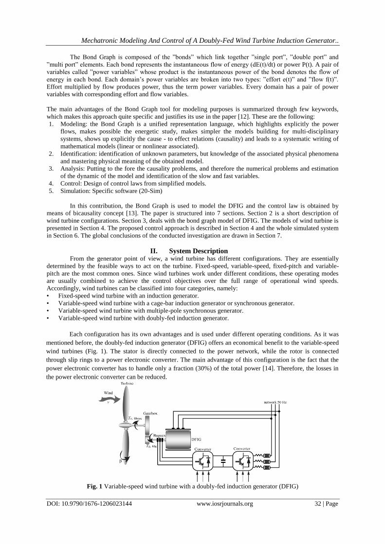
Each configuration has its own advantages and is used under different operating conditions. As it was

mentioned before, the doubly-fed induction generator (DFIG) offers an economical benefit to the variable-speed

wind turbines (Fig. 1). The stator is directly connected to the power network, while the rotor is connected

through slip rings to a power electronic converter. The main advantage of this configuration is the fact that the

power electronic converter has to handle only a fraction (30%) of the total power [14]. Therefore, the losses in

the power electronic converter can be reduced.

Fig. 1 Variable-speed wind turbine with a doubly-fed induction generator (DFIG)



III. DFIG Bond Graph model The DFIG model has been discussed in many publications [15, 16]. We can distinguish two modeling

approaches for the DFIG: on the one hand, models that use the natural reference frame (abc), and, on the other

hand models with the use of the Park reference frame (dq). The choosing of the model depends upon the type of

analysis to be conducted on the system. It is important to mention that Park reference frame models are the most

used (linear models), because a linear analysis can be implemented in an easier way, and, a DFIG features a set

of complicated equations in the natural reference frame abc. The complexity arises from the fact that the mutual

inductance matrix [Lm] varies even when the speed is in steady state. In this paper, the DFIG is presented in the

Park reference frame.

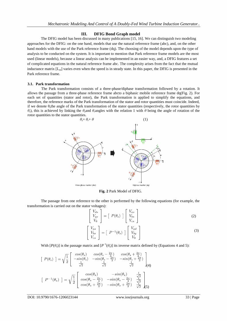
3.1. Park transformation

The Park transformation consists of a three-phase/diphase transformation followed by a rotation. It

allows the passage from a three-phase reference frame abcto a biphasic mobile reference frame dq(Fig. 2). For

each set of quantities (stator and rotor), the Park transformation is applied to simplify the equations, and

therefore, the reference marks of the Park transformation of the stator and rotor quantities must coincide. Indeed,

if we denote θsthe angle of the Park transformation of the stator quantities (respectively, the rotor quantities by

θr), this is achieved by linking the θsand θrangles with the relation 1 with θ being the angle of rotation of the

rotor quantities to the stator quantities.

θs= θr+ θ (1)

Fig. 2 Park Model of DFIG.

The passage from one reference to the other is performed by the following equations (for example, the

transformation is carried out on the stator voltages):

(2)

(3)

With [P(θs)] is the passage matrix and [P−1

(θs)] its inverse matrix defined by (Equations 4 and 5):

(4)

(5)



These previous equations can also be applied to any other quantities such as currents and

fluxes.Translation of this transformation (Equations 2 and 3) as a Bond Graph is shown in Fig. 3.

Fig. 3Park Bond Graph model.

3.2. Bond Graph model of the DFIG

The induction machine model is based on the following assumptions:

• Magnetic hysteresis and magnetic saturation effects are neglected.

• The stator windings are sinusoidally distributed along the airgap.

• The stator slots cause no appreciable variation of the rotor inductances with rotor position.

• An arbitrary dq-frame rotating around the homopolar 0-axis to the speed ωsis chosen.

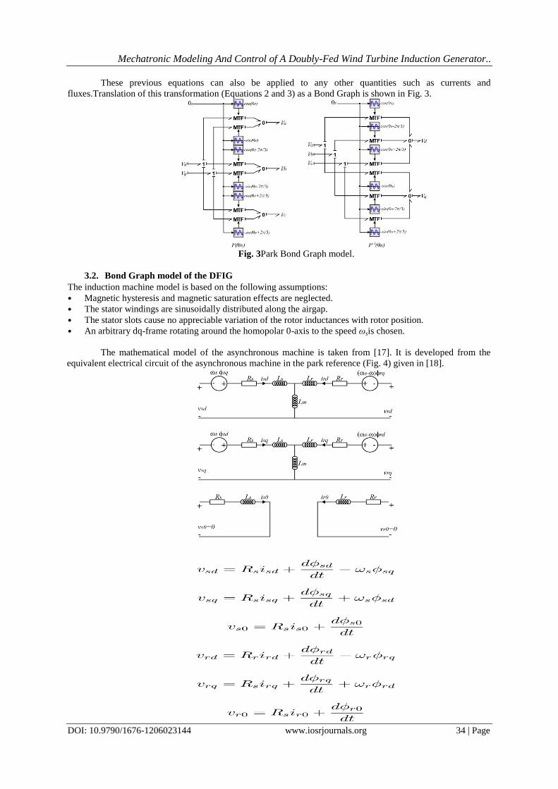
The mathematical model of the asynchronous machine is taken from [17]. It is developed from the

equivalent electrical circuit of the asynchronous machine in the park reference (Fig. 4) given in [18].



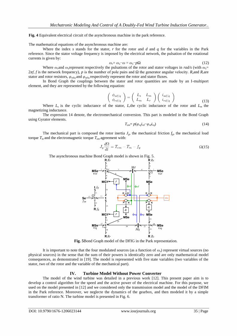
Fig. 4 Equivalent electrical circuit of the asynchronous machine in the park reference.

The mathematical equations of the asynchronous machine are:

Where the index s stands for the stator, r for the rotor and d and q for the variables in the Park

reference. Since the stator voltage frequency is imposed by the electrical network, the pulsation of the rotational

currents is given by:

ωr= ωs−ω = ωs−pΩ (12)

Where ωrand ωsrepresent respectively the pulsations of the rotor and stator voltages in rad/s (with ωs=

2πf, f is the network frequency), p is the number of pole pairs and Ω the generator angular velocity. Rsand Rrare

stator and rotor resistors, φrd/q and φsd/q respectively represent the rotor and stator fluxes.

In Bond Graph the couplings between the stator and rotor quantities are made by an I-multiport

element, and they are represented by the following equation:

(13)

Where Ls is the cyclic inductance of the stator, Lrthe cyclic inductance of the rotor and Lm the

magnetizing inductance.

The expression 14 denote, the electromechanical conversion. This part is modeled in the Bond Graph

using Gyrator elements.

Tem= p(φrqird−φrdirq) (14)

The mechanical part is composed the rotor inertia Jg, the mechanical friction fg, the mechanical load

torque Tm and the electromagnetic torque Tem agreement with:

Ω(15)

The asynchronous machine Bond Graph model is shown in Fig. 5.

Fig. 5Bond Graph model of the DFIG in the Park representation.

It is important to note that the four modulated sources (as a function of ωs) represent virtual sources (no

physical sources) in the sense that the sum of their powers is identically zero and are only mathematical model

consequences, as demonstrated in [19]. The model is represented with five state variables (two variables of the

stator, two of the rotor and the variable of the mechanical part).

IV. Turbine Model Without Power Converter The model of the wind turbine was detailed in a previous work [12]. This present paper aim is to

develop a control algorithm for the speed and the active power of the electrical machine. For this purpose, we

used on the model presented in [12] and we considered only the transmission model and the model of the DFIM

in the Park reference. Moreover, we neglecte the dynamics of the gearbox, and then modeled it by a simple

transformer of ratio N. The turbine model is presented in Fig. 6.



Fig. 6 wind turbine Bond Graph model.

The model of the wind turbine without power converter has several inputs and outputs. The wind speed

V is, of course, an input and is used to calculate the wind turbine torque (Ta). The mechanical torque (Tm) of the

turbine and the electromechanical torque (Tem) coming from the DFIG are in opposition and this generate a

rotation speed corresponding to the angular velocity of the DFIG rotor. The other inputs of the wind turbine

without power converter corresponds to the DFIG stator voltage, i.e. vsd, vsqand ωsand the rotor voltage vrdand

vrq. As for the outputs, they correspond to the stator measurements of the DFIG which include stator currents

isdand isq. The next step is to develop a law control based on the Bond Graph formalism of the DFIG in order to

control the wind turbine speed.

V. Dfig Model Control There are several control strategies for the asynchronous machine:

• The scalar control.

• The vector-oriented control.

• Direct torque and flow control.

The scalar control [20, 21] arises from the sinusoidal expressions of the asynchronous machine. The

most common strategy for this type of control is the use of a constant ratio (vs/fs) to maintain a quasi-constant

magnetic flux inside the machine. This method is simple and inexpensive. On the other hand, the dynamic

performances of this one are bad since this control is based on the DFIG steady state expressions.

Unlike the scalar control, vector control [20, 21] allows decoupling of magnetic flux and

electromechanical torque within the asynchronous machine. The flow and torque control are therefore

independent of each other. This approach is analogous to the control of a DC machine. This has the advantage of

avoiding machine flux saturation and getting a dynamic response. The vector control can be indirect or direct

and in each case, many configurations are possible. Direct vector control with oriented flux is similar to indirect

control except that it uses a flux (flux observer) estimator. This makes it possible to follow the flux evolution in

the machine, to get higher dynamic performances and to improve the control robustness with respect to machine

parameters variations. For direct torque and flow control, it requires a torque and flow observer, for example, a

Kalman filter or a Luenberger observer. Two relays and a switching table process the torque and flux errors. The

latter generates the optimum voltage to be applied to the asynchronous machine. The dynamic performance of

this control is very good and is comparable to that of the vector control. On the other hand, the use of relays

produces vibrations in the electromagnetic torque.

For the present study, direct vector oriented flow control with velocity sensor was used based upon the

Inverse Bond Graph (IBG)approach. This choice was made further to the fact that this technique is used

regularly in the industry for the control of DFIGs.

5.1. Vector control stratigy description

The basic idea of vector control with oriented flow is to independently control both the magnetic flux

and the electromagnetic torque within the DFIG. And since the DFIG can be manipulated via its stator and its

rotor, then, with the application of a rotor voltage, it must be possible to control both the torque and the flux.

The simplest way to achieve this is to carry out the vector control in the reference dq (Park reference) and to

make the axis q coincide with the rotor flux. In other words, to properly choose the angle of rotation of Park so

that the rotor flux is entirely carried on the direct axis d and thus to have φrq= 0, therforeφr= φrd(Fig. 7). Thus, if



the rotor flux phiris held constant, then the electromagnetic torque would very much resemble that of an MCC

(Expression 16). Thus, it is necessary to regulate the flux by acting on the component vdrof stator voltage and we

regulate the torque by acting on the component vqr. For this purpose, a specific algorithm is designed, based on

Bond Graph Bicausal (Inverss Bond Graph).

Tem= −pφrdirq (16)

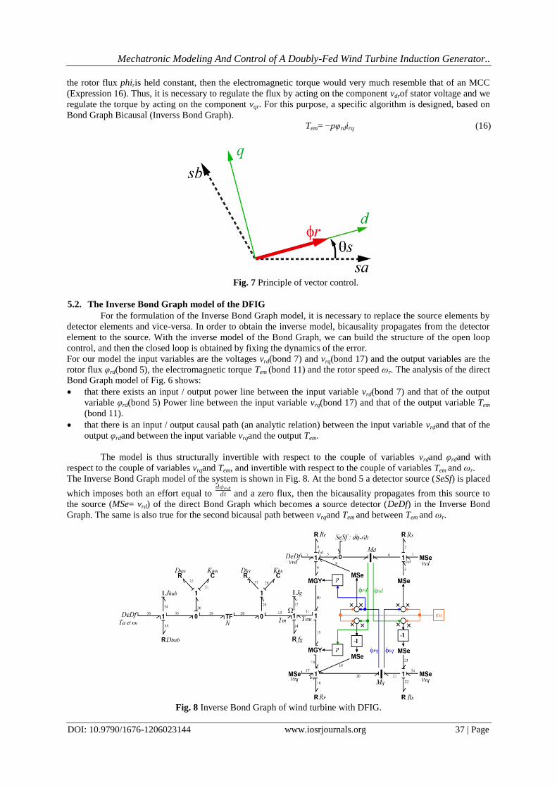
Fig. 7 Principle of vector control.

5.2. The Inverse Bond Graph model of the DFIG

For the formulation of the Inverse Bond Graph model, it is necessary to replace the source elements by

detector elements and vice-versa. In order to obtain the inverse model, bicausality propagates from the detector

element to the source. With the inverse model of the Bond Graph, we can build the structure of the open loop

control, and then the closed loop is obtained by fixing the dynamics of the error.

For our model the input variables are the voltages vrd(bond 7) and vrq(bond 17) and the output variables are the

rotor flux φrd(bond 5), the electromagnetic torque Tem (bond 11) and the rotor speed ωr. The analysis of the direct

Bond Graph model of Fig. 6 shows:

that there exists an input / output power line between the input variable vrd(bond 7) and that of the output

variable φrd(bond 5) Power line between the input variable vrq(bond 17) and that of the output variable Tem

(bond 11).

that there is an input / output causal path (an analytic relation) between the input variable vrdand that of the

output φrdand between the input variable vrqand the output Tem.

The model is thus structurally invertible with respect to the couple of variables vrdand φrdand with

respect to the couple of variables vrqand Tem, and invertible with respect to the couple of variables Tem and ωr.

The Inverse Bond Graph model of the system is shown in Fig. 8. At the bond 5 a detector source (SeSf) is placed

which imposes both an effort equal to and a zero flux, then the bicausality propagates from this source to

the source (MSe= vrd) of the direct Bond Graph which becomes a source detector (DeDf) in the Inverse Bond

Graph. The same is also true for the second bicausal path between vrqand Tem and between Tem and ωr.

Fig. 8 Inverse Bond Graph of wind turbine with DFIG.



5.3. Formulation of the control law based on the inverse model of the DFIG

The control law is determined by extracting the control equations from the Inverse Bond Graph model

of Fig. 8. For the law control of the rotor flux, the following constitutive relations can be written: from the 1-

junction placed between the bonds 5, 6, 7, 8, and 9 we have:

(17)

With e5= dφrd/dt, e6= Rrird, e7= vrd, e8= ωsφrqand e9= pφrqΩ, we have φrq= 0 therefore:

(18)

To establish the closed loop control law, the dynamics of the error is defined by the Equation 19:

= 0 (19)

Where k1 represents the controller to use and is the error.The Expression 18 becomes

20 as follows:

(20)

Finally

(21)

In the same way, the torque control law can be calculated. Equation 22 is derived from the Inverse

Bond Graph from the 1-junction between the bonds 16, 17, 18, 19 and 20.

(22)

With e17= vrq, e18= Rrir, e19= −ωsφrdand therfor:

(23)

To establish the closed-loop control law, the dynamics of the error for the current irqis defined by ˙

= 0 . Where k2 represents the controller to use and , then the Expression 23 becomes 27.

(24)

From the MGY-element, we can write:

(25)

From the 1-junction placed between the bonds 10, 11 and 15 we can write:

(26)

We can write Tem−ref = −pφrdirq−ref, so the Expression 27 becomes:

(27)

From the 1-junction placed between the bonds 11, 12, 13 and 14 we have:

(28)

Where: . Therfor:

(29)

From the 0-junction placed between bonds 13, 25 and 28, we have:

(30)

Where (from the 1-junction placed between bonds 25, 26 and 27):

(31)

Proceeding in the same way, from the TF-element we can write:

)



(32)

For the 0-junction between bonds 29, 30 and 33 we can write:

(33)

From the 1-jonction between bonds 30, 31 and 32 we have:

(34)

From the leftmost 1-junction (i.e. 1-junction placed between bonds 33, 34, 35, and 36):

(35)

where: e36 = Ta; e34 = Jhubω˙r; e35 = Dhubωr. Therefore:

(36)

To establish the closed loop control law, the dynamics of the error are set in Equation 36 as:

= 0 (37)

Where k3 represents the controller to be used and , is the error.Expression 36 becomes 38 as:

(38)

Finally,

(39)

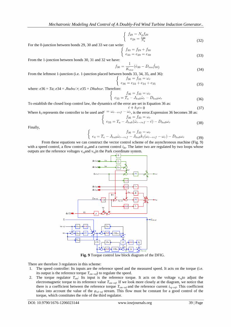
From these equations we can construct the vector control scheme of the asynchronous machine (Fig. 9)

with a speed control, a flow control φrdand a current control ids. The latter two are regulated by two loops whose

outputs are the reference voltages vrqand vrqin the Park coordinate system.

Fig. 9 Torque control law block diagram of the DFIG.

There are therefore 3 regulators in this scheme:

1. The speed controller: Its inputs are the reference speed and the measured speed. It acts on the torque (i.e.

its output is the reference torque Tem−ref) to regulate the speed.

2. The torque regulator Tem: Its input is the reference torque. It acts on the voltage vrqto adjust the

electromagnetic torque to its reference value Tem−ref. If we look more closely at the diagram, we notice that

there is a coefficient between the reference torque Tem−ref and the reference current irq−ref. This coefficient

takes into account the value of the φrd−ref stream. This flow must be constant for a good control of the

torque, which constitutes the role of the third regulator.

)



3. The flow regulator φrd: It takes as input the reference flow φrd−ref and its measurement through the currents

irdand isd. It acts on the voltage vrdto guarantee a constant rotor flux.

Reference parameters are generated using the MPPT method presented in[22].

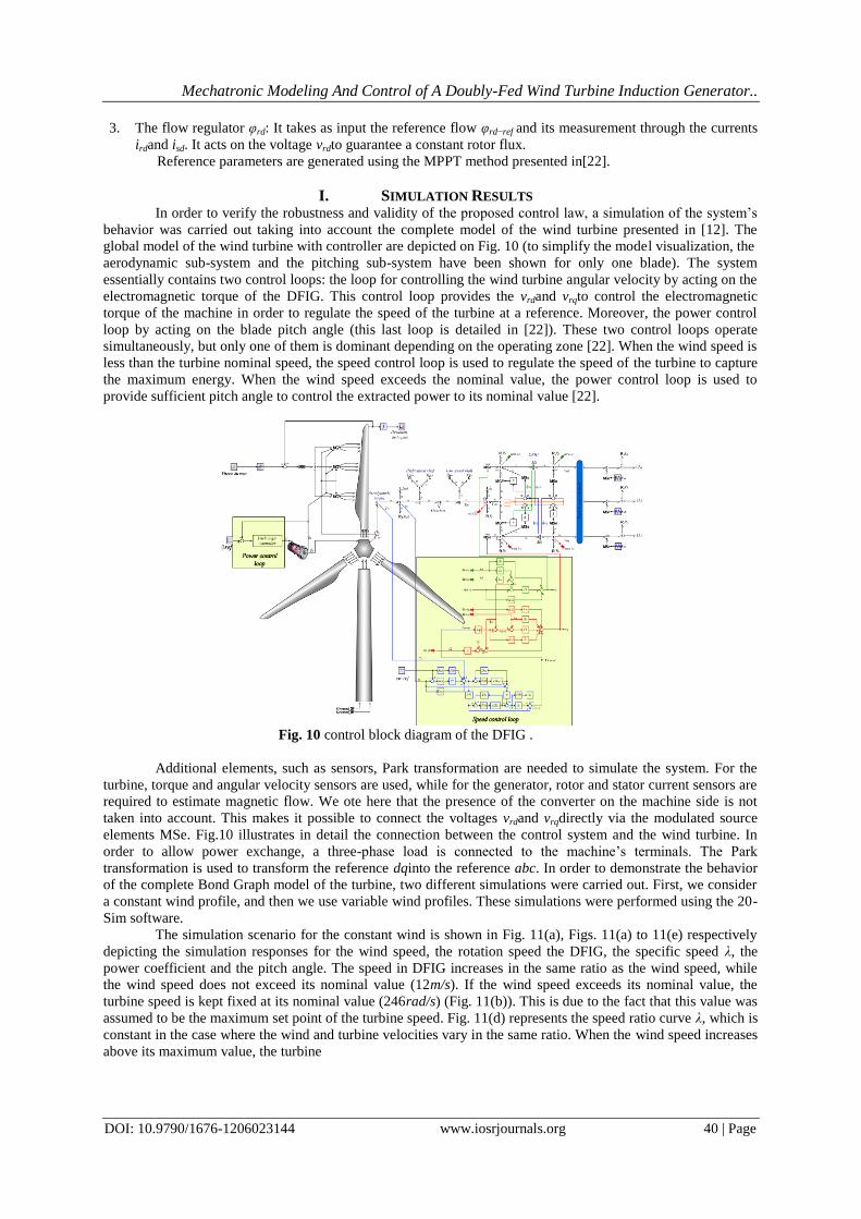
I. SIMULATION RESULTS In order to verify the robustness and validity of the proposed control law, a simulation of the system’s

behavior was carried out taking into account the complete model of the wind turbine presented in [12]. The

global model of the wind turbine with controller are depicted on Fig. 10 (to simplify the model visualization, the

aerodynamic sub-system and the pitching sub-system have been shown for only one blade). The system

essentially contains two control loops: the loop for controlling the wind turbine angular velocity by acting on the

electromagnetic torque of the DFIG. This control loop provides the vrdand vrqto control the electromagnetic

torque of the machine in order to regulate the speed of the turbine at a reference. Moreover, the power control

loop by acting on the blade pitch angle (this last loop is detailed in [22]). These two control loops operate

simultaneously, but only one of them is dominant depending on the operating zone [22]. When the wind speed is

less than the turbine nominal speed, the speed control loop is used to regulate the speed of the turbine to capture

the maximum energy. When the wind speed exceeds the nominal value, the power control loop is used to

provide sufficient pitch angle to control the extracted power to its nominal value [22].

Fig. 10 control block diagram of the DFIG .

Additional elements, such as sensors, Park transformation are needed to simulate the system. For the

turbine, torque and angular velocity sensors are used, while for the generator, rotor and stator current sensors are

required to estimate magnetic flow. We ote here that the presence of the converter on the machine side is not

taken into account. This makes it possible to connect the voltages vrdand vrqdirectly via the modulated source

elements MSe. Fig.10 illustrates in detail the connection between the control system and the wind turbine. In

order to allow power exchange, a three-phase load is connected to the machine’s terminals. The Park

transformation is used to transform the reference dqinto the reference abc. In order to demonstrate the behavior

of the complete Bond Graph model of the turbine, two different simulations were carried out. First, we consider

a constant wind profile, and then we use variable wind profiles. These simulations were performed using the 20-

Sim software.

The simulation scenario for the constant wind is shown in Fig. 11(a), Figs. 11(a) to 11(e) respectively

depicting the simulation responses for the wind speed, the rotation speed the DFIG, the specific speed λ, the

power coefficient and the pitch angle. The speed in DFIG increases in the same ratio as the wind speed, while

the wind speed does not exceed its nominal value (12m/s). If the wind speed exceeds its nominal value, the

turbine speed is kept fixed at its nominal value (246rad/s) (Fig. 11(b)). This is due to the fact that this value was

assumed to be the maximum set point of the turbine speed. Fig. 11(d) represents the speed ratio curve λ, which is

constant in the case where the wind and turbine velocities vary in the same ratio. When the wind speed increases

above its maximum value, the turbine



Fig. 11 Responses for a constant wind profile.

speed is constant and therefore the speed ratio decreases from 8 to 7m/s and then remains constant

since both velocities are kept constant. A similar case is shown for the power coefficient Cp(Fig. 11(c). The Fig.

11(e) also shows the pitch angle applied to the blades, which begins to vary at the moment when the wind speed

exceeds its nominal value (12m/s). The reference torque provided by the control law is compared with the

actualtorque in the generator (Fig. 12). These two curves agree closely; Only a small difference was identified

during the transitional phase. It is important to note that the noise presented in the simulation has no significant

impact on the behavior of the control law. This noise effect is present in all responses.

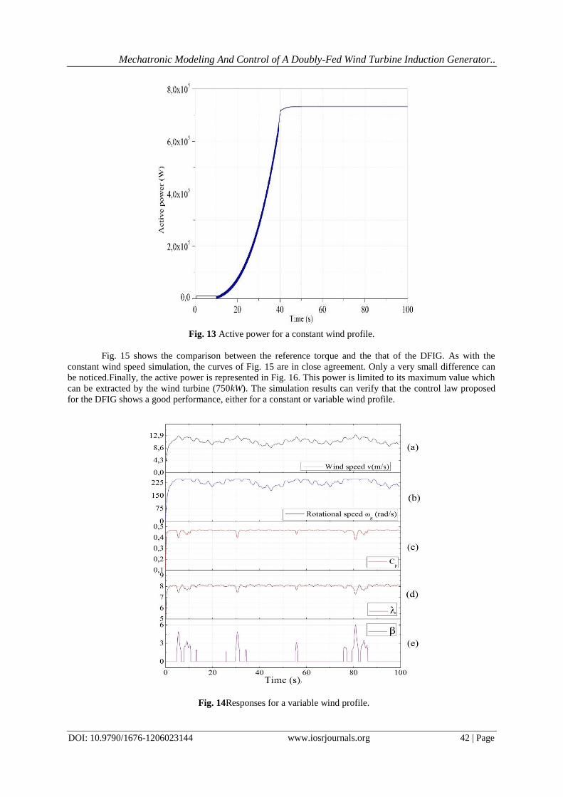
The power transferred to the grid is the most important parameter to be taken into account in a wind

turbine. Fig. 13 represents the active power supplied to the power grid. We note that the power does not exceed

its nominal value during the simulation process. It is important to mention that an initial condition of the rotation

speed of the DFIG is used to allow simulation. The simulation results for the constant wind profile validate the

theoretical concepts related to the dynamic operation of the wind turbine. In reality the wind is a stochastic

parameter of fluctuating nature, the second simulation was carried out for a variable wind profile as shown in

Fig. 14(a). Figs. of 14(b) through 14(e) schematize the simulation response for the selected wind turbine

variables. The DFIG speed varies in the same ratio as the wind speed when the wind speed does not exceed its

nominal value. When the wind speed passes through the nominal value (12 m / s) for small periods,the DFIG

speed reaches its nominal value (226rad/s). The same behavior is represented in the Cpcurve (Fig. 14(c) and the

λ curve (Fig. 14(d). The power control loop goes into action when the wind speed exceeds its nominal value.

This is shown in Fig. 14(e) which depicts the pitch angle variation during the simulation process.

Fig. 12 Reference and DFIM torques for a constant wind profile.



Fig. 13 Active power for a constant wind profile.

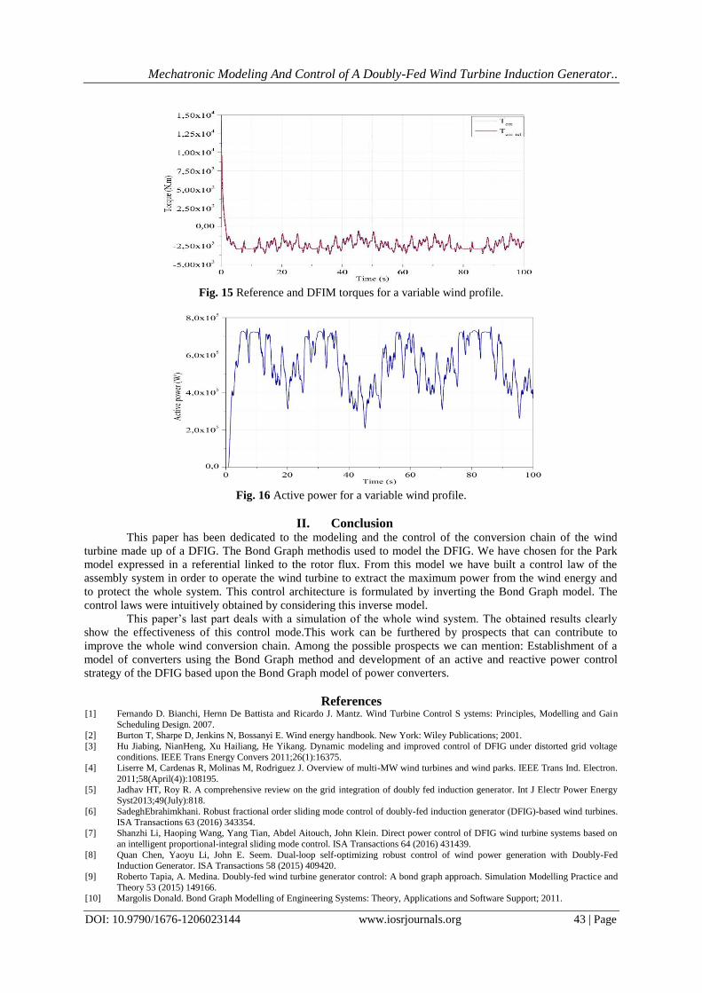
Fig. 15 shows the comparison between the reference torque and the that of the DFIG. As with the

constant wind speed simulation, the curves of Fig. 15 are in close agreement. Only a very small difference can

be noticed.Finally, the active power is represented in Fig. 16. This power is limited to its maximum value which

can be extracted by the wind turbine (750kW). The simulation results can verify that the control law proposed

for the DFIG shows a good performance, either for a constant or variable wind profile.

Fig. 14Responses for a variable wind profile.



Fig. 15 Reference and DFIM torques for a variable wind profile.

Fig. 16 Active power for a variable wind profile.

II. Conclusion This paper has been dedicated to the modeling and the control of the conversion chain of the wind

turbine made up of a DFIG. The Bond Graph methodis used to model the DFIG. We have chosen for the Park

model expressed in a referential linked to the rotor flux. From this model we have built a control law of the

assembly system in order to operate the wind turbine to extract the maximum power from the wind energy and

to protect the whole system. This control architecture is formulated by inverting the Bond Graph model. The

control laws were intuitively obtained by considering this inverse model.

This paper’s last part deals with a simulation of the whole wind system. The obtained results clearly

show the effectiveness of this control mode.This work can be furthered by prospects that can contribute to

improve the whole wind conversion chain. Among the possible prospects we can mention: Establishment of a

model of converters using the Bond Graph method and development of an active and reactive power control

strategy of the DFIG based upon the Bond Graph model of power converters.

References [1] Fernando D. Bianchi, Hernn De Battista and Ricardo J. Mantz. Wind Turbine Control S ystems: Principles, Modelling and Gain

Scheduling Design. 2007. [2] Burton T, Sharpe D, Jenkins N, Bossanyi E. Wind energy handbook. New York: Wiley Publications; 2001.

[3] Hu Jiabing, NianHeng, Xu Hailiang, He Yikang. Dynamic modeling and improved control of DFIG under distorted grid voltage

conditions. IEEE Trans Energy Convers 2011;26(1):16375. [4] Liserre M, Cardenas R, Molinas M, Rodriguez J. Overview of multi-MW wind turbines and wind parks. IEEE Trans Ind. Electron.

2011;58(April(4)):108195.

[5] Jadhav HT, Roy R. A comprehensive review on the grid integration of doubly fed induction generator. Int J Electr Power Energy Syst2013;49(July):818.

[6] SadeghEbrahimkhani. Robust fractional order sliding mode control of doubly-fed induction generator (DFIG)-based wind turbines.

ISA Transactions 63 (2016) 343354. [7] Shanzhi Li, Haoping Wang, Yang Tian, Abdel Aitouch, John Klein. Direct power control of DFIG wind turbine systems based on

an intelligent proportional-integral sliding mode control. ISA Transactions 64 (2016) 431439.

[8] Quan Chen, Yaoyu Li, John E. Seem. Dual-loop self-optimizing robust control of wind power generation with Doubly-Fed Induction Generator. ISA Transactions 58 (2015) 409420.

[9] Roberto Tapia, A. Medina. Doubly-fed wind turbine generator control: A bond graph approach. Simulation Modelling Practice and

Theory 53 (2015) 149166. [10] Margolis Donald. Bond Graph Modelling of Engineering Systems: Theory, Applications and Software Support; 2011.



[11] MerzoukiRochdi, SamantarayArun Kumar, Pathak Pushparaj Mani, OuldBouamamaBelkacem. Intelligent mechatronic systems:

modeling, control and diagnosis. 2013. [12] Zakaria Khaouch, Mustapha Zekraoui, JamaaBengourram, Nourreeddine Kouider, Mustapha Mabrouki. Mechatronic modeling of a

750 kW fixedspeed wind energy conversion system using the Bond Graph Approach. ISA Transactions 65 (2016) 418436.

[13] P.J. Gawthrop, Bicausal bond graph, in: Proceeding of the International Conference on Bond Graph Modeling and Simulation ICBGM95, vol. 27, 1995, pp. 8388.

[14] L. Xu, C. Wei, Torque and reactive power control of a doubly fed induction machine by position sensorless scheme, IEEE Trans.

Ind. Appl. 31 (3) (1995) 636642. [15] B. Umesh, L. Umanand. 2008. Bond graph model of doubly fed three phase induction motor using the Axis Rotator element for

frame transformation. Simulation Modelling Practice and Theory, vol. 16, issue 10, pp. 1704-1712.

[16] S. Junco. 1999. Real-and Complexe-Power Bond Graph Modeling of the Induction Motor. Proc. ICBGM99. San Francisco, vol. 31, No. 1, pp. 323328.

[17] S. Junco. 1999. Real-and Complexe-Power Bond Graph Modeling of the Induction Motor. Proc. ICBGM99. San Francisco, vol. 31,

No. 1, pp. 323328. [18] P.C. Krause, O. Wasynczuk, S.D. Sudhoff. 2002. ’Analysis of Electric Machinery and Drive Systems’. A John Wiley & Sons, Inc.

Publications, Second Edition.

[19] S. Junco, Real-and complexe-power bond graph modeling of the induction motor, in: Proc. ICBGM99, San Francisco, vol. 31, No. 1, 1999, pp. 323328.

[20] J. S. Thongam, Commande de haute performance sans capteur d’une machine asynchrone, Dpartement d’ingnierie, Universit du

Qubec Chicoutimi (UQAC), Chicoutimi, Juin 2006. [21] Boldeaet S. A. Nasar, Electric Drives, 2e ed, CRC Press, 2005.

[22] Zakaria Khaouch, Mustapha Zekraoui, Nourreeddine Kouider,MustaphaMabrouki, JamaaBengourram. Mechatronic Modeling and

Control of a Nonlinear Variable-Speed Variable-Pitch Wind Turbine by Using the Bond Graph Approach. Journal of Electrical and Electronics Engineering (IOSR-JEEE). Volume 11, Issue 6 Ver. I (Nov.Dec. 2016), PP 95-115. DOI:10.9790/1676-11060195115.

Zakaria Khaouch"Mechatronic Modeling And Control of A Doubly-Fed Wind Turbine Induction

Generator Using The Bond Graph Approach” IOSR Journal of Electrical and Electronics

Engineering (IOSR-JEEE), vol. 12, no. 6, 2017, pp. 31-44

IOSR Journal of Electrical and Electronics Engineering (IOSR-JEEE) is UGC approved Journal

with Sl. No. 4198, Journal no. 45125.

mechatronic modeling and control of a doubly-fed … issue 6/version-2...mechatronic modeling and...

Documents