mechanism of hip dysplasia and identification of the least
TRANSCRIPT

University of Central Florida University of Central Florida
STARS STARS
Electronic Theses and Dissertations, 2004-2019
2015
Mechanism of Hip Dysplasia and Identification of the Least Mechanism of Hip Dysplasia and Identification of the Least
Energy Path for its Treatment by using the Principle of Stationary Energy Path for its Treatment by using the Principle of Stationary
Potential Energy Potential Energy
Mohammed Abdulwahab M. Zwawi University of Central Florida
Part of the Mechanical Engineering Commons
Find similar works at: https://stars.library.ucf.edu/etd
University of Central Florida Libraries http://library.ucf.edu
This Doctoral Dissertation (Open Access) is brought to you for free and open access by STARS. It has been accepted
for inclusion in Electronic Theses and Dissertations, 2004-2019 by an authorized administrator of STARS. For more
information, please contact [email protected].
STARS Citation STARS Citation Zwawi, Mohammed Abdulwahab M., "Mechanism of Hip Dysplasia and Identification of the Least Energy Path for its Treatment by using the Principle of Stationary Potential Energy" (2015). Electronic Theses and Dissertations, 2004-2019. 1418. https://stars.library.ucf.edu/etd/1418

MECHANISM OF HIP DYSPLASIA AND IDENTIFICATION OF THE LEAST ENERGY PATH FOR ITS TREATMENT BY USING
THE PRINCIPLE OF STATIONARY POTENTIAL ENERGY
by
MOHAMMED A. ZWAWI
B.S. King Abdulaziz University, 2005 M.S. University of Central Florida, 2012
A dissertation submitted in partial fulfillment of the requirements for the degree of Doctor of Philosophy
in the Department of Mechanical and Aerospace Engineering in the College of Engineering and Computer Science
at the University of Central Florida Orlando, Florida
Fall Term 2015
Major Professor: Faissal Moslehy

ii
© 2015 Mohammed Zwawi

iii
ABSTRACT
Developmental dysplasia of the hip (DDH) is a common newborn condition where
the femoral head is not located in its natural position in the acetabulum (hip socket).
Several treatment methods are being implemented worldwide to treat this abnormal
condition. One of the most effective methods of treatment is the use of Pavlik Harness,
which directs the femoral head toward the natural position inside the acetabulum.
This dissertation presents a developed method for identifying the least energy
path that the femoral head would follow during reduction. This is achieved by utilizing a
validated computational biomechanical model that allows the determination of the
potential energy, and then implementing the principle of stationary potential energy.
The potential energy stems from strain energy stored in the muscles and gravitational
potential energy of four rigid-body components of lower limb bones. Five muscles are
identified and modeled because of their effect on DDH reduction. Clinical observations
indicate that reduction with the Pavlik Harness occurs passively in deep sleep under the
combined effects of gravity and the constraints of the Pavlik Harness.
A non-linear constitutive equation, describing the passive muscle response, is
used in the potential energy computation. Different DDH abnormalities with various
flexion, abduction, and hip rotation angles are considered, and least energy paths are
identified. Several constraints, such as geometry and harness configuration, are
considered to closely simulate real cases of DDH.
iv
Results confirm the clinical observations of two different pathways for closed
reduction. The path of least energy closely approximated the modified Hoffman-Daimler
method. Release of the pectineus muscle favored a more direct pathway over the
posterior rim of the acetabulum. The direct path over the posterior rim of the acetabulum
requires more energy. This model supports the observation that Grade IV dislocations
may require manual reduction by the direct path. However, the indirect path requires
less energy and may be an alternative to direct manual reduction of Grade IV infantile
hip dislocations. Of great importance, as a result of this work, identifying the minimum
energy path that the femoral head would travel would provide a non-surgical tool that
effectively aids the surgeon in treating DDH.

v
To my parents (Abdulwahab and Noor), my wife (Lujain), my big boy (Abdulelah),
and my little daughter (Aseel), I am presenting this work on behalf of your support
and your patience during the past three years. You always encourage me, pray for
me, push me to do something that can help mankind, and I succeeded. I wish from
my deep heart with my results the physicians can improve the treatment of the babies
with hip dysplasia.

vi
ACKNOWLEDGMENT
First of all, I am grateful to the Almighty Allah for establishing me to complete and
succeed in this research.
I would like to thank King Abdulaziz University for giving me the opportunity to
study and live in the United States during my research. Also, I would like to express my
sincere gratitude to the Department of Mechanical and Aerospace Engineering for
letting me fulfill my dream of getting my doctoral degree. This study was supported in
part by the National Science Foundation under Grant number CBET-1160179, and the
International Hip Dysplasia Institute.
To my committee, Professor Alain Kassab, Professor Hansen Mansy, and Professor
Eduardo Divo, I am extremely grateful for your assistance and suggestions throughout my
research. To Dr. Charles Price, I am glad that I worked with you during this research, and I wish
to continue our work on this manner to support humanity for a better life. To my colleague,
Christopher Rose, I am thankful for your help and support.
Most of all, I am fully thankful to my advisor Professor Faissal A. Moslehy for his full
support, understanding, patience, and encouragement during my research. I progressed quickly
with high performance and quality due to his inspiration. It was a journey that had many
difficulties and limits, but with these types of professors, I was guided to pass through all these
challenges and merge the mechanical science with the medical one to help the affected babies.

vii
TABLE OF CONTENTS
LIST OF FIGURES .......................................................................................................... x
LIST OF TABLES .......................................................................................................... xiv
CHAPTER 1: INTRODUCTION ....................................................................................... 1
1.1 Background ........................................................................................................ 1
1.2 Motivation ........................................................................................................... 7
1.3 Thesis Overview ................................................................................................. 7
CHAPTER 2: LITERATURE REVIEW ............................................................................. 9
CHAPTER 3: METHODOLOGY .................................................................................... 28
3.1 Model ............................................................................................................... 28
3.1.1 SolidWorks Model .................................................................................. 28
3.1.2 Muscle Model ......................................................................................... 32
3.1.3 Muscle Mechanics .................................................................................. 35
3.1.4 Model Scaling Factor Verification ........................................................... 38
3.1.5 Constraints ............................................................................................. 40
3.2 Energy Method ................................................................................................. 44
3.2.1 Strain Energy.......................................................................................... 45
3.2.2 Gravitational Potential Energy ................................................................ 53
3.2.3 Stationary Potential Energy .................................................................... 54
viii
3.3 Potential Energy Calculation ............................................................................ 56
3.3.1 Proper Orthogonal Decomposition (POD) .............................................. 56
3.3.2 Genetic Algorithm Code and Eureqa Software ....................................... 59
3.3.3 MATLAB Code ....................................................................................... 59
3.4 Dijkstra’s Algorithm and Least Energy Path Method ........................................ 60
CHAPTER 4: RESULTS ................................................................................................ 63
4.1 Two Angle Model ............................................................................................. 63
4.1.1 Potential Energy Calculation .................................................................. 63
4.1.2 Potential Energy Function and Local Minima ......................................... 65
4.1.3 Potential Energy Map ............................................................................. 71
4.1.4 Two Angle Model Results ....................................................................... 72
4.2 Three Angle Model ........................................................................................... 79
4.2.1 Potential Energy Calculation and Local Minima ..................................... 80
4.2.2 Potential Energy Map for the Model with Three Angles of Rotation ....... 81
4.2.3 Three Angle Model Results .................................................................... 82
CHAPTER 5: DISCUSSION AND CONCLUSION ...................................................... 106
5.1 Discussion ...................................................................................................... 106
5.2 Conclusion ..................................................................................................... 107
5.3 Future Work ................................................................................................... 109

ix
APPENDIX A: COLLISION DETECTION ALGORITHM .............................................. 111
APPENDIX B: GENETIC ALGORITHM ....................................................................... 116
Appendix B1: Genetic Algorithm Code: .................................................................... 117
Appendix B2: The Chromosome: ............................................................................. 123
LIST OF REFERENCES ............................................................................................. 126

x
LIST OF FIGURES
Figure 1 International Hip Dysplasia Institute grades, a) grading lines, b) four grades [6]
........................................................................................................................................ 3
Figure 2 Pavlik Harness as a treatment for the hip dysplasia [9]. .................................... 4
Figure 3 Femoral head in contact with the pelvis surface................................................ 6
Figure 4 Direct reduction pathway identified by Iwasaki using the Pavlik harness, and for
manual reduction. .......................................................................................................... 16
Figure 5 Reduction steps with using the Hoffman-Daimler method. .............................. 19
Figure 6 Local and global energy minima. ..................................................................... 21
Figure 7 Initial 3D model, a) hip and bones, b) adductor muscles in the model [5]. ...... 29
Figure 8 Hip model and its reference model of 14-years old female on the left [9]. ....... 30
Figure 9 Femur model and its reference model of 38-years old male on the left [47]. ... 31
Figure 10 3D model of the lower limb bones with SolidWorks. ...................................... 32
Figure 11 Five adductor muscles (Pectineus, Adductor Brevis, Adductor Longus,
Adductor Magnus, and Gracilis) [53]. ............................................................................ 34
Figure 12 Adductor Magnus Muscle divided into three different muscles [53]. .............. 35
Figure 13 The behavior of active and passive forces on the muscles [60]. ................... 36
Figure 14 Hill-Based three-element muscle model [55]. ................................................ 37
Figure 15 Adductor Magnus Minimus muscle length as a function of flexion and
abduction angles (OpenSim). ........................................................................................ 39
Figure 16 The femoral head in a spherical shape [9]. ................................................... 41
Figure 17 Flexion angle range between 70˚ and 130˚, a) 70˚, and b) 130˚. .................. 42

xi
Figure 18 Abduction angle range between 0˚ and 90˚, a) 0˚, and b) 90˚. ...................... 43
Figure 19 Hip rotation angle, (a) external rotation, and (b) internal rotation. ................. 44
Figure 20 Points located on the wireframe of the surface by using SolidWorks®. ........ 45
Figure 21 Heaviside function chart. ............................................................................... 46
Figure 22 Origin and insertion points for the Pectineus muscle. ................................... 47
Figure 23 First transformation about the flexion angle. ................................................. 48
Figure 24 Second transformation about the abduction angle. ....................................... 49
Figure 25 Third transformation about the hip rotation angle. ......................................... 49
Figure 26 Height “X” of the center of gravity for lower extremity bones. ........................ 54
Figure 27 Energy path. .................................................................................................. 55
Figure 28 Eigenvalues are sorted. ................................................................................ 57
Figure 29 The absolute energy difference of the path. .................................................. 61
Figure 30 Dijkstra’s algorithm sample window to find the hip dysplasia reduction path. 62
Figure 31 Points located on the acetabulum surface. ................................................... 64
Figure 32 Points located on the pelvis surface. ............................................................. 65
Figure 33 POD results show the potential energy at the specific femoral head location to
get the minimum energy. ............................................................................................... 66
Figure 34 Acetabulum surface that has two regions, the top one, and the bottom one. 67
Figure 35 Pelvis first region. .......................................................................................... 68
Figure 36 Pelvis second region. .................................................................................... 68
Figure 37 Pelvis third region. ......................................................................................... 69
Figure 38 Pelvis fourth region. ...................................................................................... 69
xii
Figure 39 Eureqa curve fitting data for acetabulum surface. ......................................... 70
Figure 40 Potential energy map for the model with two angles of rotation. ................... 72
Figure 41 International Hip Dysplasia Institute classification of Grade I. ....................... 73
Figure 42 Grade I: Hip Dysplasia reduction path. .......................................................... 74
Figure 43 International Hip Dysplasia Institute classification of grade II. ....................... 75
Figure 44 Grade II: Hip Dysplasia reduction path. ......................................................... 75
Figure 45 International Hip Dysplasia Institute classification of grade III. ...................... 76
Figure 46 Grade III: Hip Dysplasia reduction path. ........................................................ 76
Figure 47 International Hip Dysplasia Institute classification of grade IV. ..................... 77
Figure 48 Grade IV: Hip dysplasia reduction path. ........................................................ 79
Figure 49 Potential energy map. ................................................................................... 81
Figure 50 Grade I: Hip Dysplasia reduction path with using three angles of rotation. ... 83
Figure 51 Grade II: Hip Dysplasia reduction path with using three angles of rotation. .. 84
Figure 52 Grade III: Hip Dysplasia reduction path with using three angles of rotation. . 85
Figure 53 Grade IV: Hip Dysplasia direct reduction pathway for the model with all
muscles intact. .............................................................................................................. 87
Figure 54 Potential energy map for the direct reduction path for the model with all
muscles intact. .............................................................................................................. 87
Figure 55 Grade IV direct reduction path with femur orientation for the model with all
muscles. ........................................................................................................................ 90
Figure 56 Grade IV: Hip Dysplasia direct reduction path for the model without the effect
of the Pectineus. ........................................................................................................... 91

xiii
Figure 57 Potential energy map for the direct reduction path for the model without the
effect of the Pectineus muscle. ..................................................................................... 92
Figure 58 Grade IV direct reduction path with femur orientation for the model without the
effect of the Pectineus. .................................................................................................. 93
Figure 59 Grade IV: Hip Dysplasia indirect reduction pathway with the effect of all
muscles. ........................................................................................................................ 96
Figure 60 Potential energy map for the indirect reduction path for the model with all
muscles intact. .............................................................................................................. 96
Figure 61 Grade IV: indirect reduction path with femur orientation for the model with all
muscles intact. .............................................................................................................. 99
Figure 62 Grade IV: Hip Dysplasia indirect reduction path without the effect of the
Pectineus. ................................................................................................................... 100
Figure 63 Potential energy map for the indirect reduction path for the model without the
effect of the Pectineus muscle. ................................................................................... 101
Figure 64 Grade IV indirect reduction paths with femur orientation for the model without
the effect of the Pectineus. .......................................................................................... 104
xiv
LIST OF TABLES
Table 1 Muscle length and scaling factor between OpenSim and SolidWorks model. .. 40
Table 2 The scaled muscles’ cross-sectional areas from the OpenSim model. ............ 53
Table 3 Source points and target point definition. ......................................................... 62
Table 4 Sample of acetabulum points with local minimum potential energy at flexion and
abduction angles. .......................................................................................................... 66
Table 5 Sample of Genetic Algorithm results. ............................................................... 71
Table 6 Grade IV hip dysplasia reduction path and orientation. .................................... 78
Table 7 Sample table of the MATLAB code results of several femoral head points. ..... 80
Table 8 Grade I: required femur orientation for the hip dysplasia reduction. ................. 82
Table 9 Grade II: required femur orientation for the hip dysplasia reduction. ................ 83
Table 10 Grade III: required femur orientation for the hip dysplasia reduction. ............. 84
Table 11 Grade IV: required femur orientation for the hip dysplasia reduction (Direct
path) with the effect of all muscles. ............................................................................... 86
Table 12 Grade IV: required femur orientation for the hip dysplasia direct reduction of
the model without the effect of the Pectineus. ............................................................... 91
Table 13 The difference between the two cases in the first analysis (Direct path). ....... 94
Table 14 Grade IV: required femur orientation for the hip dysplasia indirect reduction
pathway of the model with all muscles intact. ................................................................ 95
Table 15 Grade IV: required femur orientation for the hip dysplasia indirect reduction
path of the model without the effect of the Pectineus. ................................................. 100
Table 16 The difference between the third and fourth analysis (indirect path). ........... 104

xv
Table 17 Least energy path with the required femur orientation for the model with all
muscles to follow the proposed pathway by Iwasaki. .................................................. 105
Table 18 The difference between the second and the fifth analysis (Direct pathway). 105

1
CHAPTER 1: INTRODUCTION
When the femoral head is dislocated and placed somewhere outside of its
natural position in the acetabulum (hip socket), the femur with lower limb bones will be
in a non-equilibrium condition due to muscle forces acting on these bones. This non-
equilibrium condition is called hip dysplasia. Hip dysplasia is one of the most abnormal
conditions in newborn babies. It is a common condition requiring treatment in
approximately 1% to 3% of newborn infants. One in six may demonstrate neonatal
instability while complete dislocation occurs in approximately 0.1% to 0.3% of live births.
During the growth of the baby intrauterine, particularly at eleventh week, the hip joints
will be fully formed where the hip dislocation may occur. In 1832-1834, Dupuytren was
the first to establish the lack of development of the acetabulum, and later it was referred
to by others as dysplasia [1].
The causes of hip dysplasia are unknown to researchers till now, but there are
some factors that increase the probabilities, and it is widely believed that this condition
is developmental. Some researchers have discussed the causes. According to Seringe,
et al. [2], there are two categories of causes: constitutional factors and mechanical
factors. One constitutional factor can be considered the insufficient depth of the
acetabulum. Additionally, a shallow acetabulum could be regarded as a constitutional
factor that increases the probability of dislocation. Furthermore, the mechanical factors
can be attributed to several causes. The causes are when babies are born in the breech
1.1 Background

2
presentation, born with high weight, or born with a mechanical deformation of the foot or
knee. Traditional swaddling techniques could be considered as one of the mechanical
factors that increases the possibility of hip dislocation.
The clinical sign of hip dysplasia is a clicking sound at birth for certain cases.
This click is a clear evidence of slight or moderate dysplasia. However, the sign for
severe dislocation (the femoral head is dislocated superiorly to the acetabulum) is the
abnormal limitation of the abduction of the hip [1]. On the other hand, the Ortolani Sign
can be an evidence of hip dysplasia. Originally, the link between the femoral head and
the acetabulum is loosened, and the femoral head can be made to slide in and out of
the acetabulum [3]. These factors contribute to the femoral head being dislocated from
the acetabulum, or the one that is dislocated can be relocated back inside the
acetabulum. The physicians usually do this kind of diagnosis at birth. If either diagnosis
is missed at birth, the nature of the hip could follow one of the four scenarios as
introduced by Weinstein. The hip can become normal, it can go on to subluxation or
partial contact, it can go on to complete dislocation, or it can remain located but retain
dysplastic features [4].
Developmental Dysplasia of the Hip develops after birth and affects 1 in 20
infants and should be treated within the first six months [5]. There are several hip
dysplasia classifications that are defined by the International Hip Dysplasia Institute
(IHDI) and are called grades. Hence, IHDI defined four grades of the hip dysplasia, as
displayed in Figure 1, and the most common hip dysplasia grades are 3 and 4.
3
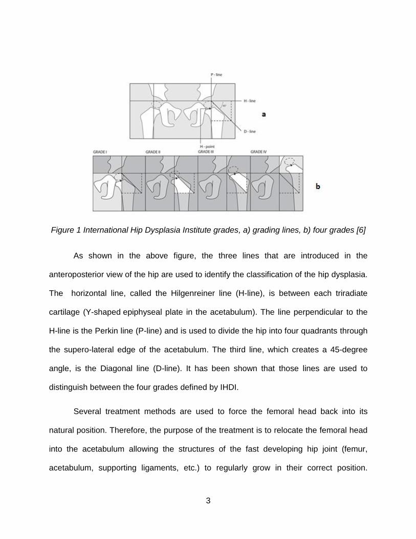
Figure 1 International Hip Dysplasia Institute grades, a) grading lines, b) four grades [6]
As shown in the above figure, the three lines that are introduced in the
anteroposterior view of the hip are used to identify the classification of the hip dysplasia.
The horizontal line, called the Hilgenreiner line (H-line), is between each triradiate
cartilage (Y-shaped epiphyseal plate in the acetabulum). The line perpendicular to the
H-line is the Perkin line (P-line) and is used to divide the hip into four quadrants through
the supero-lateral edge of the acetabulum. The third line, which creates a 45-degree
angle, is the Diagonal line (D-line). It has been shown that those lines are used to
distinguish between the four grades defined by IHDI.
Several treatment methods are used to force the femoral head back into its
natural position. Therefore, the purpose of the treatment is to relocate the femoral head
into the acetabulum allowing the structures of the fast developing hip joint (femur,
acetabulum, supporting ligaments, etc.) to regularly grow in their correct position.
4
Different treatment methods are considered for patients that have hip dysplasia. One of
the most effective methods is the Pavlik Harness. Most of the newborn babies with
dislocated hips can be treated magnificently when the harness is correctly used. It can
be used for most of the hip dysplasia grades and has become an accepted worldwide
treatment. The success rate with the Pavlik Harness and other methods depends on the
severity of dislocation and initiation age of treatment. Early detection may improve the
treatment, but severity remains an impediment to successful treatment with non-surgical
methods [7].
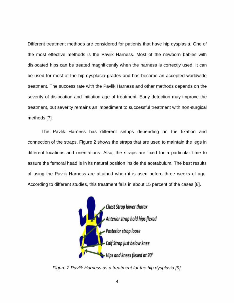
The Pavlik Harness has different setups depending on the fixation and
connection of the straps. Figure 2 shows the straps that are used to maintain the legs in
different locations and orientations. Also, the straps are fixed for a particular time to
assure the femoral head is in its natural position inside the acetabulum. The best results
of using the Pavlik Harness are attained when it is used before three weeks of age.
According to different studies, this treatment fails in about 15 percent of the cases [8].
Figure 2 Pavlik Harness as a treatment for the hip dysplasia [9].

5
In this dissertation, the principle of stationary potential energy is used to identify
the optimal path for the surgeon during the hip dysplasia reduction. Thus, the femoral
head will be successfully vectored into its correct physiological position in the
acetabulum. The potential energy stems from strain energy stored in the considered
muscles (Pectineus, Adductor Brevis, Adductor Longus, Adductor Magnus, and Gracilis)
and gravitational potential energy of four rigid-body components of the lower limb.
Hence, the potential energy will be introduced as a function of the pelvis surface,
muscle forces as strain energy, and gravitational potential energy. This function will be
used to find the optimal path to lead the surgeon to set up the harness and guide
him/her to move the femoral head along the pelvic surface in a specific path at a
specified femur orientation.
To identify the potential energy function with the least energy path with respect to
all factors in the hip dysplasia problem, a computer program was developed to
determine femoral head centers’ coordinates while the head is in contact with the pelvic
surface, as indicated in Figure 3.
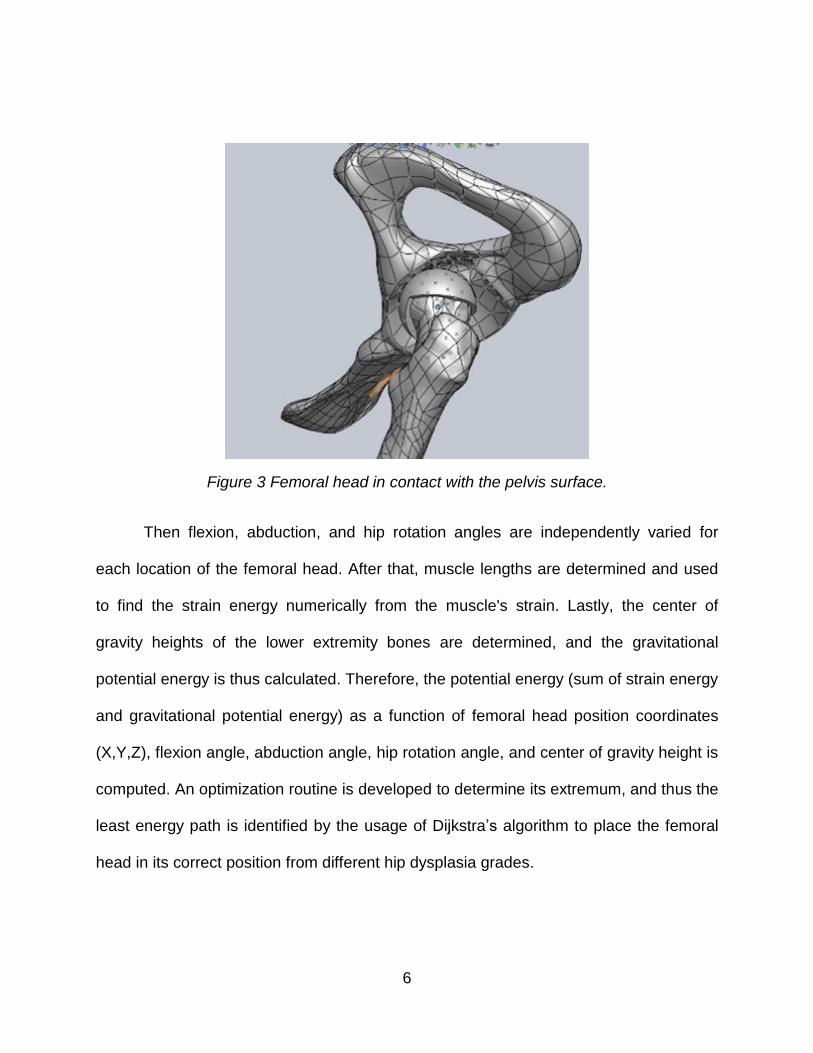
6
Figure 3 Femoral head in contact with the pelvis surface.
Then flexion, abduction, and hip rotation angles are independently varied for
each location of the femoral head. After that, muscle lengths are determined and used
to find the strain energy numerically from the muscle's strain. Lastly, the center of
gravity heights of the lower extremity bones are determined, and the gravitational
potential energy is thus calculated. Therefore, the potential energy (sum of strain energy
and gravitational potential energy) as a function of femoral head position coordinates
(X,Y,Z), flexion angle, abduction angle, hip rotation angle, and center of gravity height is
computed. An optimization routine is developed to determine its extremum, and thus the
least energy path is identified by the usage of Dijkstra’s algorithm to place the femoral
head in its correct position from different hip dysplasia grades.

7
This research defines the optimum strategy and procedure to guide the surgeon
in moving and correctly placing the femoral head in its natural position inside the
acetabulum for the four different grades with the required flexion, abduction, and hip
rotation angles along the least energy path as dictated by the principle of stationary
potential energy. The outcomes of this dissertation are the least energy paths for grades
I, II, III, and IV as described by IHDI. These pathways contain the starting point (femoral
head location during hip dislocation), the path that the femoral head should follow during
the reduction process, the required orientation of the femur (flexion, abduction, and hip
rotation angles), and the required energy for the reduction of the hip. These pathways
are considered the ones that have the least energy and could potentially improve the
treatment of the affected babies.
This dissertation has five chapters starting with the introduction chapter that has
the background of developmental of hip dysplasia, the different causes of dysplasia, the
clinical signs depending on the severity of the dysplasia, various types of treatment, and
a brief introduction of the method that is used to determine the least energy path for the
reduction process as shown previously.
The next chapter is the literature review, which contains a review of hip dysplasia
and how they diagnose it, different treatment methods and how the mechanism of each
1.2 Motivation
1.3 Thesis Overview

8
treatment works with the differences between them, the methods to find the potential
energy map, and algorithms on how to find the optimal path between two points.
The following chapter explains the three-dimensional model that has the lower
extremity bones and the corresponding muscles for the tension and movement of the
bones, the assumed constraints for the model, and the energy method to identify the
least energy path. Moreover, the muscle mechanics and introduction of the muscles are
included in this chapter and muscle mechanics as described by Fung and Hill. Finally,
the Dijkstra's algorithm is explained for the purpose of finding the least energy path.
The fourth chapter is to explain several outputs: the results of the potential
energy method, different codes were used to support the proposed method, and the
optimization method to find the pathways for all hip dysplasia grades. Lastly, the
discussion and conclusion chapter is included.

9
CHAPTER 2: LITERATURE REVIEW
The literature review in this research encompasses several areas. The first area
concerns the hip dysplasia and how it is diagnosed. The second area considers the
different treatment methods and their mechanisms. Next, two primary methods for
determining the potential energy map and algorithms for finding the optimal path
between the starting point and the destination (target) point are presented.
Weinstein, et al. [4] introduced in their study that in case developmental hip
dysplasia is not diagnosed directly after birth, the treatment will be painful, the risk will
be greater, and the benefits of treatment will be less detectable. Indeed, if the
diagnoses did not take place before six months old, the treatment and reduction will be
more difficult, and the restoration of the normal hip and femoral head inside its natural
position will be less likely. When the treatment fails, a surgical reduction operation is
required for children between the ages of six to 18 months.
One of the most effective methods of treatment is the use of the Pavlik Harness.
The word Pavlik was the family name of Professor Arnold Pavlik. In the 1950s,
Professor Pavlik introduced this harness and called it the Pavlik Harness [10, 11, 7].
The inspiration and motivation to develop his harness were because of the high rate of
avascular necrosis from conservative treatment methods and their lack of success. The
harness uses the concept of manual reduction of the hip, then maintains the hip
reduction by braces and corrects the acetabulum without the effect of avascular
necrosis of the femoral head [12].
10
The functional method of the Pavlik Harness was described by Mubarak, et al.
[12]. The seven principles that the Pavlik Harness was designed with are:
1- The reference for movement is the hip joint, and active movement should
treat it.
2- Hip and knee flexion results in the hip abduction being nonviolent and
unforced.
3- The stirrup configuration should assure hip flexion, gentle abduction, and
redirection of the femoral head into the acetabulum socket.
4- The child will determine abduction range.
5- Hygiene of the child is easy to achieve even when in the orthosis.
6- The parents and caregiver can deal with the harness directly.
7- The harness should be simple and inexpensive.
By applying this treatment method to patients at that time with the previous
principles, there were much fewer signs of avascular necrosis, and the success rate
was higher especially 100 percent for dysplasia.
V. Bialik and N. D. Reis translated a paper for Arnold Pavlik in 1989 [13]. The
topic for this translation was “Stirrups as an Aid in the Treatment of Congenital
Dysplasias of the Hip in Children”. At the time the original article was published, the
failure rate was 20 percent. The author reported that the high percentage of failures was
due to the health condition of the patients, and the treatment methods applied to them.
Pavlik defined two types of straps in his harness; the first one is stirrups for the lower

11
limb, which are tightened across the leg by two small straps, and the second strap
crosses the shoulders and is then tightened. The author explained the configuration of
the straps into four points: a) lower limb should be brought into flexion at the hip and
knee joints, b) the lower limb should be moved free in the hip joint, c) give freedom to
the flexion of the hip joints by the stirrups, d) the range of abduction should be
determined by the patient as long as the adductor muscles provide, etc. Thus, by
committing those requirements as described by the author the femoral head will be
centered in the acetabulum socket with the help of unforced abduction and suitable
flexion of the hip.
Another translation of Pavlik’s work was done by Leonard F. Peltier in 1993 [11].
The paper introduced the method of the Pavlik Harness as a treatment for congenital
hip dysplasia. Pavlik explained, that with the usage of the harness, the patients will be
prevented from extending the hip joint and all other motions will be free. He introduced
that the most important therapeutic factor in this kind of treatment was the active
movements because it eliminates the effect of the passive mechanical method of
treatment that causes femoral head necrosis. The arrangement of the harness as Pavlik
explained is two shoulder straps crossed in the back and a strap in front to keep them in
place, and the lower extremity is supported by the front strap just like a rider’s position
as shown in Figure 2. The flexion amount should be adjusted, and the foot should not
be tightened. Another adjustment is that abduction motion should be relaxed by
applying a diaper loosely. Pavlik wrote, “The relaxation of tension in the adductors
through active motion, which is the first requirement for the spontaneous reduction, is
12
regulated by the child himself”. During the abduction movement of the femoral head, the
reduction will occur when the adductors are without tension and the acetabulum are
empty.
Bin, et al. [14] wrote, “Very early Pavlik Harness therapy to ensure rapid hip
reduction and stabilization optimize the potential of the acetabulum for spontaneous
remodeling”. The author explained in his article that the treatment protocol is for the hip
to be flexed to 110 degrees and the knee to be at the level of the navel without
abduction force.
According to Stuart L. Weinstein [7], at the hospital of children in San Diego, the
treatment of newborns with hip dysplasia has a high success rate of 95%. Moreover, the
use of the Pavlik Harness for older babies achieves an 85% success of reduction, while
for children from six to nine months of age the rate of success drops. This device should
be used for the newborn babies as soon as the diagnosis of dislocation has taken place,
and for several weeks until the dislocated femoral head has localized and stabilized in
its natural position in the acetabulum. This treatment may be used for an average of
three months full-time and one more month part-time.
Another study that was conducted on the usage of the Pavlik Harness was done
by Mubarak, et al. [15]. The work was to review the results of treating 18 patients with
congenital dysplasia, subluxation, or dislocation of the hips. The most common problem
was the failure of reduction. There were many reasons for failure as indicated in the
article, and the most significant one was the improper use of the Pavlik Harness in the

13
treatment stage. However, the most important factor in the management of the hip
dysplasia is that adduction and extension of the hip should be prevented while allowing
flexion, abduction, and hip rotation. The author recommended a few points to achieve a
high quality of treatment. First, the back straps should be crossed to prevent them from
sliding over each other. The second recommendation is that the buckles for the anterior
straps should be located at the child's anterior axillary line. Third, the buckles for the
posterior straps should be located over the scapula. Fourth, the Velcro strap for the
lower limb of the leg should be located just below the child's popliteal fossa. With this
application, the results from the Pavlik Harness will be sufficient.
Kitoh, et al. [8] examined 221 hips of 210 patients. The results from his study
were that 81.9% of the hips were reduced. In this study, they concluded that the best
result of using the Pavlik Harness is when the abduction is more than 60 degrees. The
harness was applied with hip flexed at 90 to 100 degrees. The posterior straps were
laid-back enough for the knees to come to the midline in the position of the hip flexion.
According to Grill, et al. [16], the success of treatment of hip dysplasia with the
Pavlik Harness is superior to others. The study was conducted for 3,611 hips, and the
reduction rate was high. The author described the method behind the harness that two
shoulder straps were crossed on the back and fixed by a front strap. Furthermore, there
are two straps to hold the legs in slings, and the hip is flexed to more than 90 degrees
with limited the extension, which will be kept by an anterior strap. The femur adduction
should be prevented by the posterior strap, which will stop the crossing of the lower limb
to the midline.
14
More studies of the hip dysplasia treatment were conducted by Guille, et al. [17].
They found that if the Pavlik Harness treatment were carried out at early ages for the
babies, the reduction of the dysplasia is satisfactory. Moreover, Peled, et al. [18] studied
the Pavlik Harness treatment and how the stirrups work. He considered in his study
Graf III and IV, and the effect of the harness on the reduction of the hip with dysplasia.
Kalamchi, et al. [19], conducted the Pavlik Harness treatment for
122 patients over three months of age. Twenty-one patients had dislocated hips, and
101 patients were diagnosed with dysplasia, with an average age of five months old.
The results were that 97% of patients successfully achieved reduction of the hip.
Another study that supports the usage of the Pavlik Harness at an early age was
done by Atalar, et al. [20]. This study was conducted on 25 infants with a total of 31
patients with developmental dysplasia of the hip. They found that the success of the
Pavlik treatment depended on Graf type, the age of treatment, and bilaterally.
Suzuki [21] studied the effect of the Pavlik Harness on hip dysplasia reduction.
The study was recorded for nine infants with dislocation. There were two types of
dislocation. For type A, the femoral head is displaced posteriorly and lies within the
acetabulum with no contact with the anterior wall. For type B, the femoral head is in
contact with the posterior side of the socket. The results of this study for type B were
that reduction took place during deep sleep with no active movements. In type A, all six
dislocations had the head settled slowly back to the bottom of the acetabulum. The
author observed that in the manual reduction, the force to reposition the head is

15
needed, but with the usage of the Pavlik Harness, the force is generated from the
weight of the legs, so it prevents the patients from extending the hip. He specified that
this reduction was due to passive mechanical factors. Moreover, he described another
type of dislocation called type C, where the femoral head dislocated out of the
acetabulum. He concluded that in this case of dislocation, the head will not be reduced
because of the posterior wall of the acetabulum blocks the movement, so manual
reduction could force the head for reduction.
Also, Iwasaki [22] studied the mechanism of the Pavlik Harness and how the
harness allowed reduction of the hip. The Pavlik Harness moves the femoral head to
the posterior part of the acetabulum through flexion of the hip, and then moves it
anteriorly into the socket through the abduction of the hip, as illustrated in Figure 4.
Between 1966 and 1976, 240 dislocated hips of 204 patients were treated with the
Pavlik Harness, and the ages were between one and seven months. During the
treatment, the patients were frequently checked. When the neutral anteroposteriorly
made in extension with the hip showed the femoral head at the center of the
acetabulum, the hip was considered stable. After that, when the shallow acetabulum rim
was improved, the harness was removed. The knee joint was to be at 90 degrees of
flexion or more. Although, it is imperative to stretch the adductor muscles during the
treatment where the weight of the lower extremity plays the role in stretching, which will
allow the head to slide anteriorly over the acetabulum rim. The result was that 85
percent of the patients were successfully treated with the Pavlik Harness. The author

16
did a comparison with other treatment devices, and he found that the Pavlik Harness is
simple and allows movements to the lower extremity other than an extension.
Figure 4 Direct reduction pathway identified by Iwasaki using the Pavlik harness, and for
manual reduction.
Viere, et al. [23] explained in his study that the Pavlik Harness failed in some
patients with dislocated hips. The author blamed the poor application of the harness for
the cause of these failures. He agreed that it had gained widespread acceptance as a
treatment for hip dysplasia, and it has limited complications if it is used in the proper
way.

17
Abduction Orthosis is considered as an alternative method to the Pavlik Harness
treatment [7, 24]. The orthosis is appropriated for infants of more than nine months old
who require continued treatment of abduction positioning. This treatment method is
applied to patients while walking. Moreover, it is sufficient for patients up to two and half
years old. In this method of treatment, the abduction and flexion forces are transferred
mainly to the pelvis by the straps.
Seidl, et al. [25], between November 2007 and December 2010, studied and
evaluated the treatment consequences of the Tubingen hip flexion splint of newborn
patients with unstable hips. The results from Seidl’s study were a total of 50 dysplastic
or dislocated hips in 42 patients who were treated magnificently with the Tubingen splint
treatment.
Bernau [26] introduced a hip flexion splint that is used for reliable fixation of
newborn patients with an unstable hip with a flexion angle of more than 90. One more
study on the Tubingen splint was conducted by Atalar, et al. [27]. Their aim was to study
the results of using the Tubingen splint for infants with hip dysplasia. Forty-nine patients
were detected and studied. The upshots from their study were that 56 of 60 (93%) were
successfully treated with no complications. Moreover, their conclusion is that the
Tubingen provides abduction and offers advantages of preventing the hip adduction
with no constraints for the knee and ankle joints to move.
One study was conducted by Wilkinson, et al. [28], which reviewed the results of
134 patients with hip dysplasia of Graf type-III and type-IV. They were treated with the
18
Craig splint, Pavlik Harness, and Von Rosen splint. The results of this study were that
the patients treated with the Von Rosen splint are better compared to the other
harnesses. The author said, “This may be because of the difficulty in maintaining the
position of the femoral head in a very dysplastic acetabulum using the Pavlik Harness. It
is probable that a more rigid splint would be more suitable”. He mentioned that the
Pavlik Harness could be more efficient in cases of the lower dysplastic acetabulum.
Another study was by Tibrewal, et al. [10]. He studied the comparison between
different hip dysplasia treatments. The first comparison was between the Frejka pillow
and the Pavlik Harness. He found from the literature that the failure of reduction was
10% with a Frekja pillow and 12% in a Pavlik Harness. The usage of Pavlik Harness is
better when applied to patients of an age less than 24 weeks. Another comparison was
for the Craig splint, the Pavlik Harness, or the Von Rosen splint. He concluded that the
Von Rosen splint gave the best results. The author said, “an acetabular angle of 36
degrees or greater was predictive of an unsuccessful outcome” with the use of the
Pavlik Harness.
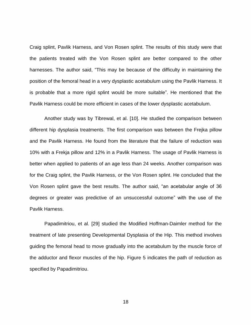
Papadimitriou, et al. [29] studied the Modified Hoffman-Daimler method for the
treatment of late presenting Developmental Dysplasia of the Hip. This method involves
guiding the femoral head to move gradually into the acetabulum by the muscle force of
the adductor and flexor muscles of the hip. Figure 5 indicates the path of reduction as
specified by Papadimitriou.
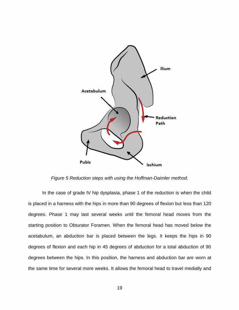
19
Figure 5 Reduction steps with using the Hoffman-Daimler method.
In the case of grade IV hip dysplasia, phase 1 of the reduction is when the child
is placed in a harness with the hips in more than 90 degrees of flexion but less than 120
degrees. Phase 1 may last several weeks until the femoral head moves from the
starting position to Obturator Foramen. When the femoral head has moved below the
acetabulum, an abduction bar is placed between the legs. It keeps the hips in 90
degrees of flexion and each hip in 45 degrees of abduction for a total abduction of 90
degrees between the hips. In this position, the harness and abduction bar are worn at
the same time for several more weeks. It allows the femoral head to travel medially and
20
then enter the acetabulum through the acetabular notch. After the hip is in the socket,
the harness is removed, but the abduction bar is kept to prevent re-dislocation. As a
conclusion, Papadimitriou said, “Late-presenting or neglected developmental dysplasia
of the hip can be successfully treated with the use of a modified Hoffmann-Daimler
method. The high rate of successful reduction, the low prevalence of osteonecrosis and
residual dysplasia, and the limited complications may make this modified method a safe
alternative to surgical treatment”.
Hip dysplasia can be studied by assuming the femur and the hip as rigid bodies
connected by spring elements (the muscles). Each muscle is modeled as a spring
having a constant “k”, initial length “Lo”, and a stretched length “L”. The corresponding
potential energy “E” can be expressed as
𝐸 =1
2𝐾(𝐿𝑜 − 𝐿)2
This assumption is derived from the potential energy surface for a diatomic
molecule [30]. However, the energy increases if the bond length “q” of the molecules is
stretched. Hence, the potential energy at the original bond length will be zero, which is
the bottom end of the parabola. Therefore, the first derivative of the energy function with
respect to each generalized parameter is the stationary potential energy.
𝜕𝐸
𝜕𝑞𝑖= 0
According to Lewars [30], there will be a global minimum potential energy and
local minima energy for the complex geometry. Figure 6 displays the global minimum

21
that has the lowest energy among the whole potential energy surface and the transition
state where the molecule moves from one minimum to another.
Figure 6 Local and global energy minima.
Huayamave [31] proposed a real-time response framework by using the Proper
Orthogonal Decomposition (POD) method. His proposal was to provide a solution that
calculates, in real-time, flow features and loads that result from wind-induced drag and
lift forces on Photo-Voltaic (PV) systems. The solutions found are organized and stored
to get the basis snapshots of POD decomposition matrix. A radial basis function (RBF)
is used for interpolation network. Moreover, it will be employed to predict the solution
from the POD decomposition, which will give a set of values of the design variables.
Both the POD snapshot matrix and RBF interpolation network are stored. This stored
data can be accessed anytime to predict the solutions.
Another study that used the POD is by Ostrowski, et al. [32]. Ostrowski was
using it for an inverse method which was developed to estimate the unknown heat
conductivity and the convective heat transfer coefficient. The POD was used here to

22
solve a sequence of direct problems within the body under consideration. Then each
problem’s solution is sampled at a matrix of a set of points. Moreover, each sampled
field is known as POD snapshot. Furthermore, POD analysis is an efficient method to
detect a correlation between the snapshots and yields a small set of orthogonal vectors
(POD basis) constituting an optimal set of approximation functions. The result from this
analysis is coefficients that are trained POD basis. Moreover, this basis is then used in
the inverse analysis, which will be restored to a condition of minimization of the
discrepancy between the measured temperatures and values calculated from the
model.
Lewars developed an algorithm, which gives the path from the starting point to
the global minimum through local minima and transition states, to optimize the
geometry. For the purpose of finding a path, all points on the grid should be adjusted to
give the lowest possible energy. Thus, for the chemical reaction, it is focused on the
minima and the passage of the molecule from one minimum to another through a
transition state. He described the potential energy surface as a plot of the energy that
gives the energy as a function of coordinates, and it is called the Born-Oppenheimer
surface. They used the first and second derivative of the energy function with respect to
the generalized parameters “𝑞𝑖".
𝐸 =1
2𝐾(𝑞 − 𝑞𝑜)
2
𝐸 − 𝐸𝑜 = 𝐾(𝑞 − 𝑞𝑜)2
23
𝜕𝐸
𝜕𝑞𝑖= 2𝐾(𝑞 − 𝑞𝑜)
𝜕𝐸2
𝜕𝑞𝑖2 = 2𝐾
Where (𝜕𝐸
𝜕𝑞𝑖), is the slope of the surface and (
𝜕𝐸2
𝜕𝑞𝑖2), is the curvature, which is the force
constant for motion along the geometrical coordinate.
Quapp, et al. [33] studied the properties of the potential energy surface by
analyzing the concept of the minimum energy path with a choice of a coordinate
system. They used the concept of potential energy surface for understanding the
chemical reaction by using transition state theory. They used the term of path of least
resistance to identify the continuous line connecting reactants and products in a
chemical reaction. Quapp said, “This path is nothing else but a mathematically defined
curve going from a higher to a lower potential”. He defined the potential energy function
as “U(x)” and the gradient “𝜕𝑈
𝜕𝑋𝑖=0” is the description of stationary points.
According to Scharfenberg [34], the stationary points on the potential energy
surface should be found by using geometry optimization methods instead of calculating
the points on the surface. Initially, they have to find the first derivative of energy with
respect to the coordinates “𝜕𝐸
𝜕𝜉𝑖= 0”, which are the stationary points, where ξi is the
geometrical coordinates. He mentioned that to increase the efficiency of the derivatives,
it is recommended to use analytical calculation rather than numerical methods. In

24
addition, to find the critical points on the surface that identify the minimum energy path,
they have to calculate the eigenvalues and eigenvectors of the constant force matrix,
which are the second derivatives of energy function with respect to geometrical
coordinates “𝜕𝐸2
𝜕𝜉𝑖2”, which is the transition states.
Smidstrup, et al. [35] proposed a method that generates an initial guess of a
transition path without evaluation of the energy. The transition path is between initial
and final states of the system. The author described the surface as a function that
interpolated pairwise distances at each discretization point along the path, which was
used to find the minimum energy path along the potential energy surface. The initial
path guess is advanced from the nudged elastic band method, which represents the
path as a discrete set of configurations for all the atoms in a chemical reaction system.
The nudged elastic band method is constructed by a linear interpolation of the
coordinate system between the initial and final states.
In chapter 8 of Schlegel [36], the author explained the potential energy surface
and its components, i.e. global minima, transition states, saddle points, path, etc. The
potential energy surface is defined as the energy surface of molecules that is a position
function of atoms or nuclei. This function can be calculated from the electron energy
and wave function for a series of fixed nuclear positions. Furthermore, when the
gradient or the first derivatives of the potential energy surface are equal to zero, the
local minima can be located. Schlegel used the concept of a matrix of second
derivatives of the potential energy surface (Hessian matrix or force constant matrix) to
25
find the saddle points and transition states. All those factors are used in an algorithm to
find the reaction path as an optimum path.
An algorithm was developed and analyzed for locating stationary points
corresponding to local minima and transition states on the potential energy surface by
Nichols, et al. [37]. The algorithm depends on the first derivative and second derivative
of the energy function with respect to geometrical constants. The author identified the
path between the minima through transition states. The method, which was proposed in
this article, uses the local slope or gradient vector and Hessian matrix as the second
derivative to find the step vector which was used to find the path on the three-
dimensional potential energy surface.
A multidimensional potential energy surface has been studied with respect to
finding transition states and the path by Basilevsky, et al. [38]. The authors used a
concept of the reaction path on the potential energy surface, and gradients with second
derivatives for local minima, saddle points, and transition states. They generated an
algorithm called “the mountaineer’s algorithm”, which formulated a method of
constructing a smooth curve linking the initial location to the destination with saddle
points. The smooth curve was called the “optimum ascent path”.
Another method for the energy path was described by Kiryati, et al. [39]. He
considered an estimation of the minimal distance and the shortest path between two
points on a continuous three-dimensional surface. They used an algorithm to compute
the shortest path with the shortest time. In a complex surface, it is better to start with an

26
initial guess to reduce the possibility of convergence to unimportant local minima. The
three-dimensional surface is digitized and continuous. This surface is digitized as a set
of voxels, which can be represented by a 6-directional chain code. By applying the
method explained in their work, they found the minimum path for separate examples.
Stefanakis, et al. [40] examined the optimum path for travel problems. They
implemented a movement algorithm on the plane surface, three-dimensional space, and
movement on a spherical surface. It has been defined that the optimal path could be
considered the shortest, least expensive, fastest, or least risky path. It was described in
their approach that they have five steps to find the optimum path. First, determine a
finite number of spots in space. Second, establish a network of those spots. Third,
produce the travel cost. Fourth, assign an accumulated travel cost to the spots. Finally,
determine the optimum path.
Another study continued and improved the method of Dijkstra’s algorithm. This
study was conducted in 1987 by Mitchell, et al. [41], and it determined the shortest path
between a source and destination points in the polyhedral surface while the path stays
on the surface. The idea was to locate the destination between the source and the
destination in the subdivision that was created by the algorithm. They tested a 3-
dimensional surface of a problem called Discrete Geodesic problem. In their theory,
they divided the surface into triangles, and they found the optimal path between two
points, not passing any point more than once. They called their algorithm the
“continuous Dijkstra”.

27
Aleksandrov, et al. [42] presented the first algorithm for computing the shortest
paths in weighted three-dimensional domains by polynomial time approximation. They
formulated their problem to calculate the path of the minimum cost from a fixed source
to any destinations in the domain surface. The cost is defined as a weighted sum of
lengths. The proposed shortest path algorithm was established by using the Voronoi
Diagram.
Kimmel, et al. [43] tried to generate an algorithm to find the shortest path. They
considered two stages in their study; the first phase is an algorithm that combines three-
dimensional length estimators with the graph, and the second phase is developed to
become a shortest geodesic curve. Those stages in this study were achieved by using
an algorithm that deforms an arbitrary initial curve ending at two points on a given
surface via geodesic curvature shortening flow. The authors mentioned in their study
that to find the shortest path between two points on a continuous surface, a numerical
solution of differential equations by numerical integration is involved. Moreover, an initial
guess is needed to increase the convergence to the global optimum path.
28
CHAPTER 3: METHODOLOGY
One of the difficulties encountered in this type of research is the lack of data for
new-born babies. To implement the study, a group of researchers developed a rigid-
body dynamic model [5]. It was generated by using SolidWorks® (Dassault Systems,
Concord, MA) from CT scans of different models and scaling them to a particular baby
model. Furthermore, a simulation software “OpenSim” (National Center for Simulation in
Rehabilitation Research, Stanford, CA) of an adult model [44], which used cadavers
with average height of 168.4 ± 9.3 cm and weight of 82.7 ± 15.2 kg [45], is used to study
the muscle lengths and behaviors due to femur orientation and to verify the solid model
from SolidWorks®. More importantly, the mechanics of several selected muscles is
studied for potential energy calculation. A study is done to check all the constraints that
affect the model.
3.1.1 SolidWorks Model
A group of researchers created a three-dimensional solid model that was
constructed by using the solid model software. Initially, a simplified model was
generated by the hip geometry with lower extremity bones and includes most of the
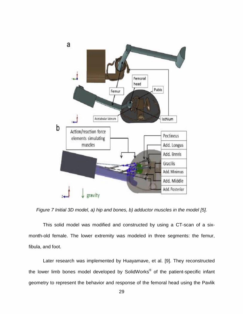
anatomical properties to carry out the analysis [5]. Figure 7 shows the detailed model
that was modified with SolidWorks®.
3.1 Model
29
Figure 7 Initial 3D model, a) hip and bones, b) adductor muscles in the model [5].
This solid model was modified and constructed by using a CT-scan of a six-
month-old female. The lower extremity was modeled in three segments: the femur,
fibula, and foot.
Later research was implemented by Huayamave, et al. [9]. They reconstructed
the lower limb bones model developed by SolidWorks® of the patient-specific infant
geometry to represent the behavior and response of the femoral head using the Pavlik

30
Harness treatment [46, 9]. This model was generated and constructed with the use of
different reference models and scaled to the size of a 10-week baby. The hip model was
developed by using a 14-year-old female with an anisotropic scaling factor (X=0.35,
Y=0.3, and Z=0.35) which matched an infant’s orthopedic data found in Hensinger’s
Standards in Pediatric Orthopedics [16], as displayed in Figure 8.
Figure 8 Hip model and its reference model of 14-years old female on the left [9].
The femur model was constructed by scaling a 38-year-old male’s femur from the
Visible Human Project of the National Library of Medicine (NLM) [47]. Thus, the femur
was scaled anisotropically (X= 0.23, Y= 0.25, and Z= 0.22) to match the 10-week-old
baby as depicted in Figure 9.
SUPERPOSITION

31
Figure 9 Femur model and its reference model of 38-years old male on the left [47].
After scaling the lower limb bones from different models as described above, the
3D model was constructed, as illustrated in Figure 10. The model includes the hip,
femur, tibia, fibula, and foot. Following, five adductor muscles were added to the solid
model [48]. Those muscles are the Pectineus, Adductor Brevis, Adductor Longus,
Adductor Magnus, and Gracilis. They have been modeled with straight lines of action.

32
Figure 10 3D model of the lower limb bones with SolidWorks.
The knee joint was flexed at 90 degrees. For this configuration, the adductor
muscles during the treatment will be stretched by the effect of the weight of the lower
extremity, which will allow the head to slide anteriorly over the acetabulum rim [22].
3.1.2 Muscle Model
In the human body, there are several tissues and one of the most functional
tissues is the muscle. Muscles and tendons actuate the movement by developing forces
and moments about the joints. Also, muscles are made of a set of muscle fascicles that
are arranged in a parallel form. Each muscle fascicle is formed from a bundle of muscle
fibers, which are a similar length in each specific muscle but vary between different
muscles [49, 50]. Thus, these fibers’ length depends on the number and length of

33
sarcomeres. Those sarcomeres are arranged in a series in the fibers, which are the
fundamental unit of force generation in the muscle [51].
Moreover, muscle tissue is considered a soft tissue. There are three types of
muscles in the body: skeletal muscles, smooth muscles, and cardiac muscles [52]. The
skeletal muscles link the skeletal bones, and then provide the action and movement of
the skeleton. Smooth muscles are different from skeletal muscles and cardiac muscles.
They can be found on the blood vessels and in the lymphatic vessels. The cardiac
muscles are in the heart walls and contract without stimulation of the neuro-central
system. Thus, the corresponding muscles for hip dysplasia studied in this research are
the skeletal muscles.
The five key adductor muscles that are considered in this research (Pectineus,
Adductor Brevis, Adductor Longus, Adductor Magnus, and Gracilis) are displayed in
Figure 11.

34
Figure 11 Five adductor muscles (Pectineus, Adductor Brevis, Adductor Longus,
Adductor Magnus, and Gracilis) [53].
The adductor muscles can adduct and produce external rotation of the hip. The
Pectineus muscle is a quadrangular muscle that is flat and located at the anterior part of
the upper and medial of the thigh. It is the most anterior adductor muscle of the hip, and
the major function of this muscle is to flex the thigh at the hip. However, the Adductor
Brevis is the muscle that connects the hip at the inferior ramus of the pubis to the thigh
at the pectineal line and the middle of the femur. Its function is to rotate the thigh and
flex it, but the prime function is to adduct the thigh at the hip. In the same way, the
Adductor Longus is located in front of the other adductor muscles on the same plane of
the Pectineus. It adducts the hip along with flexion and internal rotation. The Adductor
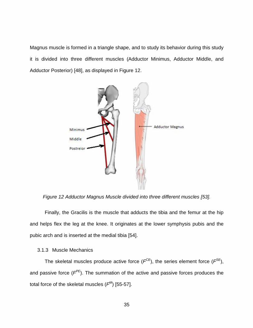
35
Magnus muscle is formed in a triangle shape, and to study its behavior during this study
it is divided into three different muscles (Adductor Minimus, Adductor Middle, and
Adductor Posterior) [48], as displayed in Figure 12.
Figure 12 Adductor Magnus Muscle divided into three different muscles [53].
Finally, the Gracilis is the muscle that adducts the tibia and the femur at the hip
and helps flex the leg at the knee. It originates at the lower symphysis pubis and the
pubic arch and is inserted at the medial tibia [54].
3.1.3 Muscle Mechanics
The skeletal muscles produce active force (FCE), the series element force (FSE),
and passive force (FPE). The summation of the active and passive forces produces the
total force of the skeletal muscles (FM) [55-57].

36
FM = FCE + FSE
FPE = FSE
The active force is generated by the interaction of actin and myosin contractile
proteins. It is generated under isometric conditions while shortening the sarcomere. The
sarcomere resting length occurs at the peak of the active tension curve. The passive
force is obtained by lengthening the muscles and is increased exponentially by
stretching the muscles [58]. This force, that starts at the sarcomere resting length, is
generated by pulling the muscle fibers, as shown in Figure 13. The characteristic
behaviors of the passive part of the muscle are a non-linear relation between stress and
strain, incompressible behavior, and large deflection [59].
Figure 13 The behavior of active and passive forces on the muscles [60].
The mechanics of Skeletal Muscles has been studied by many researchers. One
of the most well-known models is the classical three-elements Hill-Based muscle model
[61, 59], as described in Figure 14.

37
Figure 14 Hill-Based three-element muscle model [55].
The Hill-Based muscle model consists of a contractile element (CE) and two non-
linear spring elements, one in series (SE) and another in a parallel form (PE). The CE
element models the active force of the muscle. The SE element is a spring that is
responsible for the non-linear movement of the muscle and provides an energy storing
mechanism. It is also considered as a lightly-damped elastic element in series with the
contractile element. The PE element was modeled as a viscoelastic or quasi-static
elastic element, which is due to the very slow lengthening of the muscle fiber. This
element, which is defined as the passive element, handles the stretch of the muscle [60,
55].
During the hip dysplasia treatment with the usage of the Pavlik Harness, the best
results occur when the patient is asleep with no active motion [21]. According to the

38
research [22, 21, 46] in the manual reduction, the force to reposition the femoral head is
needed, but with the usage of Pavlik Harness, the force is generated from the weight of
the legs. This prevents the patients from extending the hip because the weight causes
abduction. By these means, the reduction was due to passive mechanical factor. It has
been shown that the passive force is considered the affecting force on the muscle due
to stretching.
Muscles are modeled as nonlinear force elements positioned along the line of
action of the muscles and defined by a constitutive nonlinear model named the Fung
model [62]. Lately, Magid and Law gave the final model of the muscle as below [63].
𝜎 =𝐸𝑜
𝛼(𝑒𝛼 𝜀 − 1) (1)
Where, σ is muscle stress due to deformation, Eo is muscle elastic modulus, α is
empirical constant, and ε is the muscle strain.
The muscle strain is calculated by using the reference length “Li”, which is 80% of
the relaxed length at the relaxed position, as illustrated in Figure 13 above.
3.1.4 Model Scaling Factor Verification
The OpenSim model is used to verify the reconstructed SolidWorks model which
has an anisotropic scaling factor of x=0.23, y=0.25, and z=0.22 for the femur of a 38-
year-old male from the Visible Human Project “VHP” [47] to the 10-week-old baby. The
procedure of this verification is to find the initial length of the five muscles from
OpenSim along with all possible abduction and flexion angles. The muscles’ initial

39
length (a function of abduction and flexion angles) are found from OpenSim by using the
surface chart. For example, Figure 15 shows the surface chart for the Adductor Magnus
Minimums muscle.
Figure 15 Adductor Magnus Minimus muscle length as a function of flexion and
abduction angles (OpenSim).
After finding the initial length of all muscles, the scaling factors are then varied
between 0.206 and 0.26, and they have an average scaling factor of 0.23 in the length
direction, as listed in Table 1. After a comparison of the SolidWorks model and the
OpenSim model is completed, it is found that the scale used has an average difference
of about 8.7% in the length direction.

40
Table 1 Muscle length and scaling factor between OpenSim and SolidWorks model.
Muscle Length (OpenSim)
Length (SolidWorks) @ same angles
SolidWorks initial Length
Differences in SolidWorks
Scaling factor
Pectineus 70.7 mm 18.20 mm 17.60 mm 3% 0.257
Add. Longus
170.7 mm 38.80 mm 36.37 mm 6% 0.227
Add. Brevis
114.9 mm 23.96 mm 23.79 mm 0.7% 0.208
Magnus Add. Minimus
95.3 mm 21.45 mm 20.94 mm 2.4% 0.225
Magnus Add. Middle
173.0 mm 39.88 mm 39.89 mm ≈ 0% 0.230
Magnus Add. Posterior
319.0 mm 85.53 mm 81.31 mm 5% 0.260
Gracilis 430.3 mm 87.27 mm 87.27 mm 0% 0.203
3.1.5 Constraints
There are several constraints taken in to consideration in this research. The
geometrical constraints arise from the femoral head shape and the pelvic surface. The
head, modeled as a sphere [46, 9], is depicted in Figure 16.

41
Figure 16 The femoral head in a spherical shape [9].
Moreover, the femoral head is assumed to be in contact with the pelvic surface in
all locations of the hip, as shown in Figure 3 above. Thus, the distance from the femoral
head center to the contact point is “d=7mm” (the femoral head radius).
The distance formula is used to compute the coordinates (x,y,z) of the femoral
head center.
𝑑 = √(𝑥 − 𝑥𝑖)2 + (𝑦 − 𝑦𝑖)2 + (𝑧 − 𝑧𝑖)2 (2)
Where, (𝑥𝑖 , 𝑦𝑖 , 𝑧𝑖) is the contact point on the pelvic surface.
Additionally, the harness configuration is used to constrain the ranges of the
femur orientation to be rotated about the flexion axis between 70 degrees and 130
degrees, as shown in Figure 17, within an abduction angle range of 0 degrees to 90
degrees, as illustrated in Figure 18, and with a hip rotation angle ranging between -30
degrees to +30 degrees, as depicted in Figure 19.

42
Figure 17 Flexion angle range between 70˚ and 130˚, a) 70˚, and b) 130˚.

43
Figure 18 Abduction angle range between 0˚ and 90˚, a) 0˚, and b) 90˚.

44
Figure 19 Hip rotation angle, (a) external rotation, and (b) internal rotation.
As discussed earlier, this study is based on the principle of stationary potential
energy that consists of strain energy and gravitational potential energy. The strain
energy is stored in the muscles due to the stretch from the dislocation and the rotation
in flexion, abduction, and hip rotation angles. Whereas, the gravitational potential
energy is produced by the weight of the lower extremity bones (femur, tibia, fibula, and
foot).
3.2 Energy Method

45
3.2.1 Strain Energy
The strain energy of the considered muscles is computed according to the
following procedure. First, a computer program is developed using the collision
detection algorithm, which uses vectors from the center of the sphere (femoral head) to
selected points on the pelvic surface, as illustrated in Figure 20. In this routine, the
femoral head is located in the space away from the pelvic surface and moved toward
each point on the surface while checking for any point of contact. Once the code finds
the distance “d” is equal to 7mm, it prints out the coordinates of the femoral head
center. Refer to Appendix A for details.
Figure 20 Points located on the wireframe of the surface by using SolidWorks®.
Second, by getting a grid of points from the collision detection routine, a further
calculation is conducted. At each point of the sphere center, the lengths “L” of the
selected muscles are calculated by using the distance formula between the insertion

46
and origin points on the femur and the hip. Following, the strain “ε” for all muscles is
calculated, as described in equation 3.
휀 =𝐿−𝐿𝑖
𝐿𝑖 (3)
𝐿𝑖 is the reference muscle length and is equal to 80% of the muscle’s relaxed
length “𝐿𝑟𝑒𝑙𝑎𝑥”, as shown in Figure 13 above. The relaxed lengths are assumed to be at
the fetal position of the new born baby, which is observed at 120 degrees of flexion and
20 degrees of abduction.
Because muscles can only be stretched, a Heaviside function is used to
exchange all negative values of the strain with zero value, as illustrated in Figure 21 and
equation 4. Therefore, the effective strain can be described as shown in equation 5.
Figure 21 Heaviside function chart.
𝑢(휀) = 0 𝑖𝑓 휀 < 01 𝑖𝑓 휀 > 0
(4)
휀𝑒𝑓𝑓 = 휀 ∗ 𝑢(휀) (5)
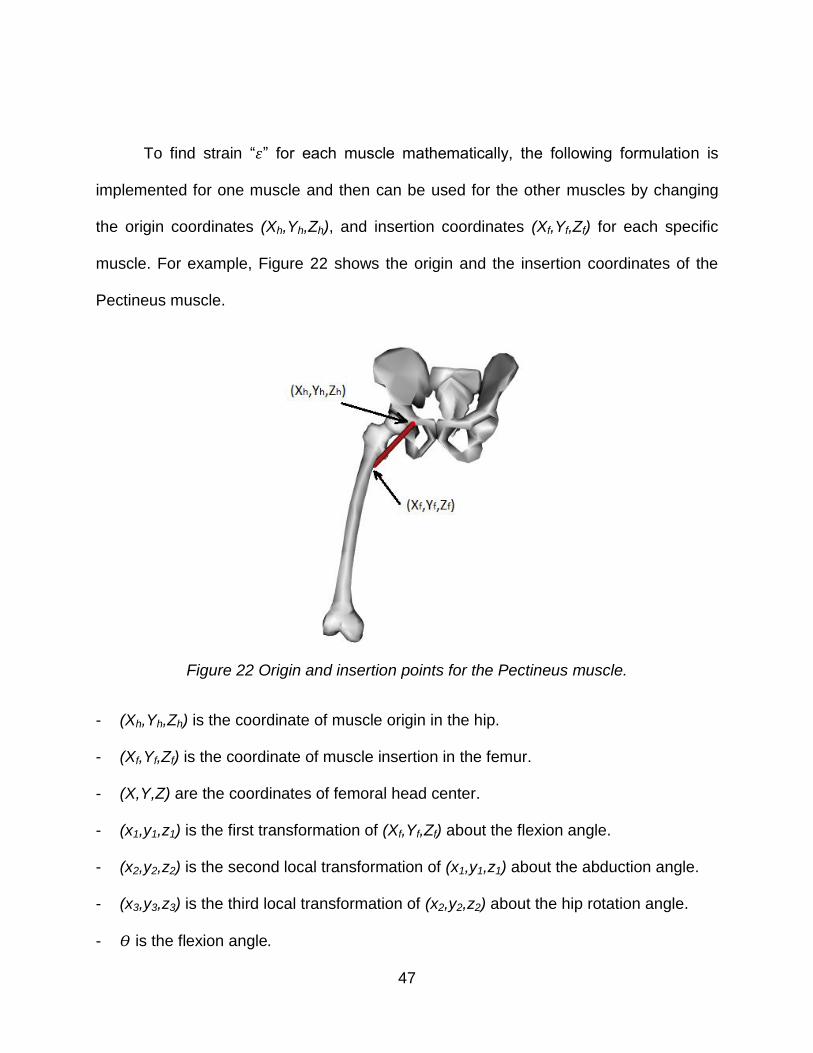
47
To find strain “휀” for each muscle mathematically, the following formulation is
implemented for one muscle and then can be used for the other muscles by changing
the origin coordinates (Xh,Yh,Zh), and insertion coordinates (Xf,Yf,Zf) for each specific
muscle. For example, Figure 22 shows the origin and the insertion coordinates of the
Pectineus muscle.
Figure 22 Origin and insertion points for the Pectineus muscle.
- (Xh,Yh,Zh) is the coordinate of muscle origin in the hip.
- (Xf,Yf,Zf) is the coordinate of muscle insertion in the femur.
- (X,Y,Z) are the coordinates of femoral head center.
- (x1,y1,z1) is the first transformation of (Xf,Yf,Zf) about the flexion angle.
- (x2,y2,z2) is the second local transformation of (x1,y1,z1) about the abduction angle.
- (x3,y3,z3) is the third local transformation of (x2,y2,z2) about the hip rotation angle.
- 𝛳 is the flexion angle.

48
- 𝛷 is the abduction angle.
- 𝜑 is the hip rotation angle.
- Lrelax is the muscle relaxed length at the relaxed position (𝛳 = 120𝑜 𝑎𝑛𝑑 𝛷 = 20𝑜) for
the new born baby.
- The first transformation is about the flexion angle of the insertion coordinate (Xf,Yf,Zf)
to the coordinate (x1,y1,z1), as shown in Figure 23.
Figure 23 First transformation about the flexion angle.
[𝑥1
𝑦1𝑧1
] = [cos𝛳 −sin𝛳 0sin𝛳 cos𝛳 0
0 0 1] [
𝑋𝑓
𝑌𝑓𝑍𝑓
] , where ϴ is the flexion angle.
𝑥1 = 𝑋𝑓. cos 𝛳 − 𝑌𝑓 . sin𝛳
𝑦1 = 𝑋𝑓 . sin𝛳 + 𝑌𝑓 . cos𝛳
𝑧1 = 𝑍𝑓 (6)
- The second transformation is about the abduction angle of the coordinate (x1,y1,z1)
to the coordinate (x2,y2,z2), as shown in Figure 24

49
Figure 24 Second transformation about the abduction angle.
[𝑥2
𝑦2𝑧2
] = [cos𝛷 0 −sin𝛷
0 1 0sin𝛷 0 cos𝛷
] [𝑥1
𝑦1𝑧1
] , where Φ is the abduction angle.
𝑥2 = 𝑥1. cos𝛷 − 𝑧1. sin 𝛷
𝑦2 = 𝑦1
𝑧2 = 𝑥1. sin𝛷 + 𝑧1. cos𝛷 (7)
- The third transformation, which is for point (x2,y2,z2), is about the hip rotation angle,
as illustrated in Figure 25.
Figure 25 Third transformation about the hip rotation angle.
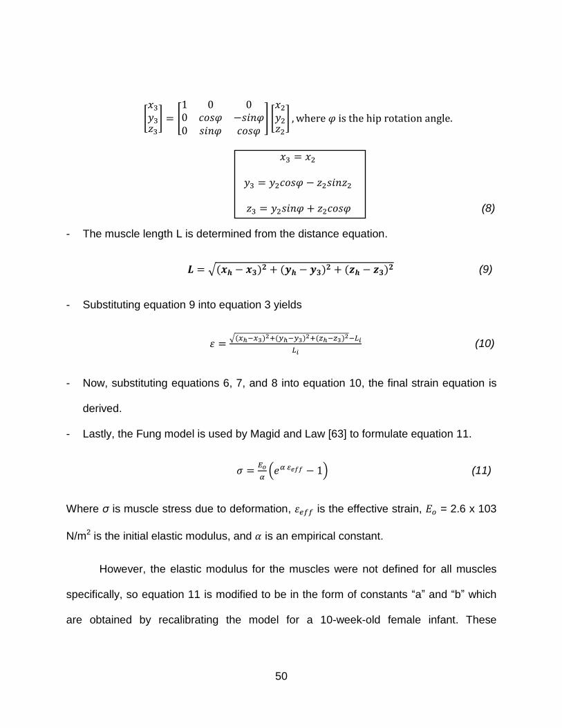
50
[𝑥3
𝑦3𝑧3
] = [1 0 00 𝑐𝑜𝑠𝜑 −𝑠𝑖𝑛𝜑0 𝑠𝑖𝑛𝜑 𝑐𝑜𝑠𝜑
] [𝑥2
𝑦2𝑧2
] , where 𝜑 is the hip rotation angle.
𝑥3 = 𝑥2
𝑦3 = 𝑦2𝑐𝑜𝑠𝜑 − 𝑧2𝑠𝑖𝑛𝑧2
𝑧3 = 𝑦2𝑠𝑖𝑛𝜑 + 𝑧2𝑐𝑜𝑠𝜑 (8)
- The muscle length L is determined from the distance equation.
𝑳 = √(𝒙𝒉 − 𝒙𝟑)𝟐 + (𝒚𝒉 − 𝒚𝟑)𝟐 + (𝒛𝒉 − 𝒛𝟑)𝟐 (9)
- Substituting equation 9 into equation 3 yields
휀 =√(𝑥ℎ−𝑥3)2+(𝑦ℎ−𝑦3)2+(𝑧ℎ−𝑧3)2−𝐿𝑖
𝐿𝑖 (10)
- Now, substituting equations 6, 7, and 8 into equation 10, the final strain equation is
derived.
- Lastly, the Fung model is used by Magid and Law [63] to formulate equation 11.
𝜎 =𝐸𝑜
𝛼(𝑒𝛼 𝜀𝑒𝑓𝑓 − 1) (11)
Where σ is muscle stress due to deformation, 휀𝑒𝑓𝑓 is the effective strain, 𝐸𝑜 = 2.6 x 10³
N/m2 is the initial elastic modulus, and 𝛼 is an empirical constant.
However, the elastic modulus for the muscles were not defined for all muscles
specifically, so equation 11 is modified to be in the form of constants “a” and “b” which
are obtained by recalibrating the model for a 10-week-old female infant. These

51
constants are used to stiffen the exponential function to stabilize the hip joint as shown
in equation 12.
𝜎 = 𝑎 (𝑒𝑏 𝜀𝑒𝑓𝑓 − 1) (12)
Thelen [56] and Delp [51] specified these two constants for the adult model as
𝑎 =𝐶
𝑒𝐾𝑃𝐸−1
= 0.466𝑁
𝑐𝑚2 (13)
𝑏 =𝐾𝑃𝐸
𝜀𝑜𝑀 = 6.667 (14)
Where, C = 25 N.cm2 is the specific muscle tension, KPE = 4 is the exponential shape
factor, and 휀𝑜𝑀 = 0.6 is the passive muscle strain.
For the 10-week-old female infant model, the value of “b” is assumed to be
13.95, and the value of “a” is recalibrated for the infant model to achieve the equilibrium
at the flexion angle of 90 degrees, abduction angle of 80 degrees, and hip rotation angle
at 0 degrees, where a = 0.00078 MPa.
Moreover, integrating the stress with respect to strain, the strain energy density
“𝑈𝑜” is determined as shown in equation 15.
𝑈𝑜 = ∫ 𝜎 𝑑휀𝜀
0 (15)
The final strain energy density is
𝑈𝑜 =𝑎
𝑏(𝑒𝑏.𝜀𝑒𝑓𝑓 − 𝑏. 휀𝑒𝑓𝑓 − 1) (16)

52
Finally, the strain energy values “U” are computed for all femoral head center
locations with variant flexion, abduction, and hip rotation angles. The strain energy
function is determined as shown in equation 17.
𝑈 = 𝑈𝑜 ∗ 𝑉 = 𝑓(𝑋, 𝑌, 𝑍, 𝛳, 𝛷, 𝜑) (17)
Where V is the volume of each muscle (V = physiological cross-sectional area *L).
To estimate the physiological cross-sectional area (PCSA) for the studied
muscles, MRI data for the Adductor Brevis of the infant model is utilized with an area of
41 mm2. In general, the PCSA is proportional to the force in the muscles, and this area
is varied along each muscle. It is calculated by dividing the volume of the muscle by the
length. Next, the PCSA of the adult Adductor Brevis muscle from the OpenSim software
is found equal to 11.52 cm2. Therefore, the scaling factor is computed between the adult
and infant models to be 3.56. This scaling factor is used to scale the PCSA of all
muscles from the OpenSim model. Table 2 lists the physiological cross-sectional areas
of the OpenSim and scaled infant models.

53
Table 2 The scaled muscles’ cross-sectional areas from the OpenSim model.
Muscle OpenSim PCSA cm2 Scaled PCSA mm2
Pectineus 9.03 32.14
Adductor Longus 22.73 80.90
Adductor Brevis 11.52 41.00
Add. Magnus Min. 25.52 90.83
Add. Magnus Mid. 18.35 65.31
Add. Magnus Post. 16.95 60.33
Gracilis 3.72 13.27
3.2.2 Gravitational Potential Energy
The second part of the potential energy calculation is to find the gravitational
potential energy value for each femoral head center’s location. This potential energy (Ω)
is the negative of the work done by the weight of the lower extremity bones (femur, tibia,
fibula, and foot). Moreover, the lower limb bones are assumed to be fixed relatively to
each other as one rigid body. The gravitational potential energy is calculated by defining
the center of gravity height “X”, as illustrated in Figure 26, for all locations on the hip
with different flexion, abduction, and hip rotation angles. Hence, the reference axis for
calculating the height is the horizontal line that passes through the acetabulum center
while the baby is lying horizontally.

54
Figure 26 Height “X” of the center of gravity for lower extremity bones.
The mass “mtotal” is the total mass of the femur, tibia, fibula, and foot. Therefore,
a computer code is modified to calculate the gravitational potential energy by changing
the location of the femoral head center and changing the femur orientation for all
possible flexion, abduction, and external rotation angles.
Ω = −𝑚𝑡𝑜𝑡𝑎𝑙. 𝑔. 𝑋 (18)
𝑚𝑡𝑜𝑡𝑎𝑙 = 0.65 𝐾𝑔
This gravitational potential energy is a function of femoral head center coordinate
(X,Y,Z), flexion angle “𝛳”, abduction angle “𝛷”, and hip rotation angle “φ”.
3.2.3 Stationary Potential Energy
The potential energy “𝛱” consists of elastic strain energy “U”, stored in the
muscles, and gravitational potential energy “Ω”, which is the work done “-W” by the
weight in the gravitational field, and it is a function of (X,Y,Z,𝛳,𝛷,φ).
𝛱(𝑋, 𝑌, 𝑍, 𝛳, 𝛷, 𝜑) = 𝑈 + Ω (19)

55
There are an infinite number of paths between any two positions 𝑟1 and 𝑟2 . The
path with least energy is the true path and leads to an equilibrium state, and the paths
with slight differences are the varied paths, as shown in Figure 27.
Figure 27 Energy path.
Furthermore, the energy path between any two positions (𝑟1 and 𝑟2 ) can be defined as
𝐸𝑃 = ∫ 𝛱 𝑑𝑟 ; 𝛱 = 𝛱(𝑋, 𝑌, 𝑍, 𝛳, 𝛷, 𝜑)𝑟2
𝑟1 (20)
Moreover, the least energy path is attained when
𝛿 ∫ 𝛱 𝑑𝑟 = ∫ 𝛿𝛱 𝑑𝑟 = 0 𝑟2
𝑟1
𝑟2
𝑟1 (21)
Thus,
𝛿𝛱 = 0 (22)
Lastly, equation 22 leads to
𝜕𝛱
𝜕𝑞𝑖= 0 (23)
Where qi are the generalized coordinates.

56
Several methods are utilized to calculate the potential energy values and to
compute the local minima of the potential energy for all femoral head center locations.
3.3.1 Proper Orthogonal Decomposition (POD)
POD is a curve fitting method. This method creates snapshots of a POD
decomposition matrix and uses radial basis functions (RBF) for creating an interpolation
network, which is used to predict the solution. Therefore, the POD and the RBF will be
stored in a database that can be accessed any time to retrieve the solutions.
The first step in this method is creating the snapshot matrix “U”, which is a
collection of N values of femoral head locations and M values of different femur
orientations. In this case, the snapshot matrix is UNxM. The goal of this matrix “U” is to
find the POD basis “Φj”, which is an orthonormal vector (j=0, 1, 2 … M), and given by
Φ = U.V (24)
Where V is eigenvectors of the covariance matrix C and can be computed by using a
nontrivial solution of the general eigenvalue problem represented as
C⋅V = Λ⋅V (25)
Where Λ is a diagonal matrix that stores the eigenvalues “λ” of matrix C, C is symmetric
and positive and can be defined as
C = UT.U (26)
Where λ is real, positive, and graphed in descending order, as shown in Figure 28.
3.3 Potential Energy Calculation
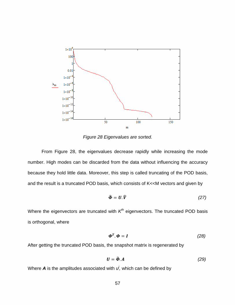
57
Figure 28 Eigenvalues are sorted.
From Figure 28, the eigenvalues decrease rapidly while increasing the mode
number. High modes can be discarded from the data without influencing the accuracy
because they hold little data. Moreover, this step is called truncating of the POD basis,
and the result is a truncated POD basis, which consists of K<<M vectors and given by
= 𝑼. (27)
Where the eigenvectors are truncated with Kth eigenvectors. The truncated POD basis
is orthogonal, where
𝜱𝑻. 𝜱 = 𝑰 (28)
After getting the truncated POD basis, the snapshot matrix is regenerated by
𝑼 = . 𝑨 (29)
Where A is the amplitudes associated with uj, which can be defined by

58
𝐀 = 𝐓. 𝐔 (30)
The data should be extrapolated by considering a vector P, which stores the
parameters of the problem, which are flexion angles “θ” and abduction angle “𝛷”. To
proceed with the extrapolation, a coefficient matrix B should be calculated from A = B⋅F,
where F is the matrix of interpolation functions, and the set of interpolation functions
“fi(p)” can be chosen arbitrarily.
𝑩 = 𝑨. 𝑭−1 (31)
For better approximation and smoothing properties, a radial basis function (RBF)
can be used as the interpolating function. Therefore, an inverse multiquadric RBF is
created and defined by
𝑓𝑖(𝒑) = 𝑓𝑖(|𝒑 − 𝒑𝑖|) =1
√|𝒑−𝒑𝑖|2+𝑐2
(32)
Where c is defined as the RBF smoothing factor and pi is parameter p at different ui (for
i = 1, 2 … M). By using all the above relations, the POD basis function can be derived
as
ΦT ⋅U = B⋅F (33)
Lastly, by using the orthogonality of the truncated POD basis, the snapshot matrix is
u(p) ≈Φ⋅B⋅F(p) (34)
Moreover, this model can be described as the trained POD-RBF network to find
any unknown data at any given parameter p. This function can be used as the curve
fitted potential energy function.

59
3.3.2 Genetic Algorithm Code and Eureqa Software
The Genetic algorithm is a well-known optimization method. It is used to find the
minimum potential energy for all femoral head center locations. At each location, the
Genetic Algorithm code is conducted to find the minimum potential energy with respect
to the flexion and abduction angles. Therefore, it is required to define the function of the
potential energy with respect to the desired variables. Eureqa software is used to find
the function of the potential energy. It uses genetic programming with symbolic
regression to determine the mathematical equation which represents the dataset.
The Genetic algorithm code, as illustrated in Appendix B1 and B2, is conducted
for each femoral head location (x,y,z) for the ranges of 70 to 130 degrees of flexion and
0 to 90 degrees of abduction. These ranges are constrained by the Pavlik Harness
straps. The code uses a random population of both angles and ranks the chromosomes
according to their fitness, and it is used to find the minimum energy values of the energy
function. Moreover, the code mates and mutates the population as per the definition
given in the code. After the process of the genetic algorithm is finished, the outputs will
be the local minima potential energy for all points with respect to the flexion and
abduction angles.
3.3.3 MATLAB Code
A MATLAB code [64] is created for calculating the potential energy values for all
femoral head center locations of the model with regards to the three angles of rotation.
First, the femoral head center location’s coordinates are defined in the code. Second,
the muscle insertion and origin coordinates are added. Third, the three-dimensional
60
rotation is applied to the insertion coordinates of the muscles to find the new position of
each insertion point. The rotation is started about the flexion angle between 70 degrees
and 130 degrees, then rotated about the abduction angle between 0 degrees and 90
degrees, and finally rotated about the hip rotation angle between -30 degrees and 30
degrees. Fourth, the mathematical model and the values of equilibrium constants “a”
and “b” are introduced into the code to calculate the potential energy values for all
locations. Lastly, the code finds the minimum energy at a specific femur orientation.
After finding the local minimum potential energy for all femoral head center
locations, Dijkstra’s algorithm code [65] is modified to find the least energy path for the
hip dysplasia reduction. First, the coordinates of all femoral head center locations (x,y,z)
are identified in the program. Second, the points’ numbers in the code for each point are
assigned. The third required input is the edges between the points, which can be
determined by addressing the adjacent points for each point. Finally, the local minimum
potential energy for all points is assigned. The program requires the source point
number and the target point number to be inputted. The program then calculates two
variables: the absolute value of the energy difference between the source point and all
adjacent points, and the distance. This process is repeated until all points in the field are
covered, and a path tree is created by the program. Finally, it picks the path of least
energy required for reduction. It should be noted that in case the paths between the
source and the target have the same amount of energy differences, which are
independent of the path, the code will check for the second condition, which is the
3.4 Dijkstra’s Algorithm and Least Energy Path Method

61
shortest path, as illustrated in Figure 29. Thus, the program will follow the same process
but for the shortest distance between the source and the target points.
Figure 29 The absolute energy difference of the path.
Figure 30 below depicts the program window of the inputs. This window has
three required inputs to be given. The first input is the file name that has the points’
numbers, the points’ coordinates, the local minima potential energy, and the adjacent
points for each point. The second input, listed in Table 3, is the number of the source
points, which is the location of the femoral head at each hip dysplasia grades’ location.
The last input is the target point number, which is the center of the acetabulum where
the femoral head should be relocated. The results from this program are each points’
number that the path goes through, the energy required for the reduction of the hip
dysplasia, and the total length between the source point and the target point.

62
Figure 30 Dijkstra’s algorithm sample window to find the hip dysplasia reduction path.
Table 3 Source points and target point definition.
Point # Definition
75 Natural location of the femoral head at the Center of the acetabulum
66 Femoral head center location at Grade I
27 Femoral head center location at Grade II
5 Femoral head center location at Grade III
131 Femoral head center location at Grade IV

63
CHAPTER 4: RESULTS
This chapter presents the results of the implemented computer codes, potential
energy map, and the optimal path for hip dysplasia reduction. Initially, the model with
two angles of rotation (flexion and abduction angles) is considered. Moreover, another
study is implemented by adding the third femur orientation (hip rotation angle). The later
investigation yielded more accurate results by determining the least energy path (LEP).
To re-iterate, there are two types of analyses carried out in this research: the first
analysis has two angles of rotation and the second one considers all three angles of
rotation.
In this section, the potential energy values for all femoral head locations are
calculated by using the mathematical model that was described in the previous chapter.
A curve fitting for the dataset of the potential energy values is conducted by using two
methods: Proper Orthogonal Decomposition (POD) and Eureqa software. Following, the
potential energy map is created by using MATLAB software. Finally, the Dijkstra’s
algorithm code is applied to find the LEP for the hip dysplasia reduction for all grades.
4.1.1 Potential Energy Calculation
In the previous chapter, the mathematical model was created to calculate the
potential energy values for all femoral head locations (i.e., acetabulum points, and
pelvis points) by using equation 19, changing flexion angles between 70 and 130
degrees and abduction angles between 0 and 90 degrees. After calculating the energy
4.1 Two Angle Model
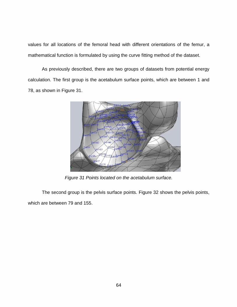
64
values for all locations of the femoral head with different orientations of the femur, a
mathematical function is formulated by using the curve fitting method of the dataset.
As previously described, there are two groups of datasets from potential energy
calculation. The first group is the acetabulum surface points, which are between 1 and
78, as shown in Figure 31.
Figure 31 Points located on the acetabulum surface.
The second group is the pelvis surface points. Figure 32 shows the pelvis points,
which are between 79 and 155.

65
Figure 32 Points located on the pelvis surface.
The next key step is to determine the potential energy function. This function will
lead to finding the local minima of potential energy, thus creating the potential energy
map and developing the LEP.
4.1.2 Potential Energy Function and Local Minima
Two results are presented in this section by using the POD and the Genetic
algorithm. After creating the POD_RBF, the local minima of the potential energy for all
femoral head locations are found. At each femoral head location, the POD plotted a
chart of the potential energy versus different angles, and the smallest value is the local
minimum energy at that location. Figure 33 shows the plot of the calculated potential
energy values for all points. Table 4 has a sample of several points of the femoral head

66
location in the acetabulum surface and the corresponding local minima of potential
energy at different flexion and abduction angles.
Figure 33 POD results show the potential energy at the specific femoral head location to get the minimum energy.
Table 4 Sample of acetabulum points with local minimum potential energy at flexion and abduction angles.
N Flexion Abduction Potential Energy (J)
1 70 84 0.20
2 70 54 0.27
3 70 48 0.32
4 70 42 0.36
5 70 30 0.40
6 70 24 0.43
7 70 12 0.45

67
The local minima of potential energy can be shown in the following figures, which
are the acetabulum surface and four regions in the pelvic area. Figure 34 displays the
corresponding flexion and abduction angles where the local minima occur at the
acetabulum points. Figure 35 shows the corresponding flexion and abduction angles
where the local minima occur at the first region of the pelvis surface. Figure 36 displays
the corresponding flexion and abduction angles where the local minima occur at the
second area of the pelvis surface. Figure 37 displays the corresponding flexion and
abduction angles where the local minima occur in the third area of the pelvis surface.
Finally, Figure 38 shows the corresponding flexion and abduction angles where the
local minima occur for the last area of the pelvic surface.
Figure 34 Acetabulum surface that has two regions, the top one, and the bottom one.

68
Figure 35 Pelvis first region.
Figure 36 Pelvis second region.

69
Figure 37 Pelvis third region.
Figure 38 Pelvis fourth region.

70
The Genetic algorithm is used to find the minimum potential energy for all
femoral head locations. Therefore, Eureqa software is used to find the function of the
potential energy. Figure 39 shows two colored points: the blue dots are the calculated
potential energy values and the red dots are the curve fitted points. Hence, the software
finds the most curve fitted data to the given values and prints out the curve fitted
function, as illustrated in equation 35 and 36.
Figure 39 Eureqa curve fitting data for acetabulum surface.
The potential energy function for the first surface points (acetabulum points) is:
𝜋1−78 = 0.5 + 0.001 ∗ 𝑧 ∗ 𝛳 + 0.0235 ∗ 𝑧 ∗ 𝛳 ∗ 𝛷 − 0.34 ∗ 𝛳 / 𝛷 + 0.001 ∗ 𝑧 ∗ 𝛷 ∗
𝛳^2 + 0.0015 ∗ 𝛷 ∗ 𝑧^2 ∗ 𝛳^2 − 0.013 ∗ 𝑧 (35)
Where, (x,y,z) is the femoral head center coordinates, 𝛳 is the flexion angle (in radian),
and 𝛷 is the abduction angle (in radian).
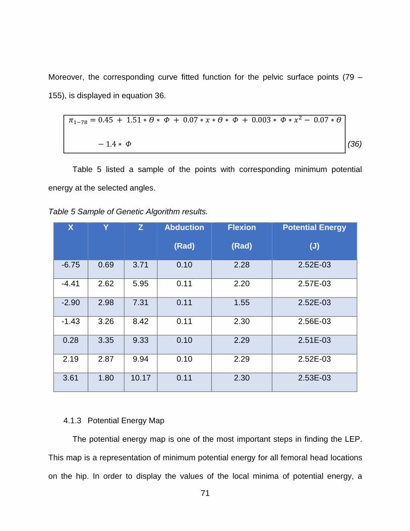
71
Moreover, the corresponding curve fitted function for the pelvic surface points (79 –
155), is displayed in equation 36.
𝜋1−78 = 0.45 + 1.51 ∗ 𝛳 ∗ 𝛷 + 0.07 ∗ 𝑥 ∗ 𝛳 ∗ 𝛷 + 0.003 ∗ 𝛷 ∗ 𝑥2 − 0.07 ∗ 𝛳
− 1.4 ∗ 𝛷 (36)
Table 5 listed a sample of the points with corresponding minimum potential
energy at the selected angles.
Table 5 Sample of Genetic Algorithm results.
X Y Z Abduction
(Rad)
Flexion
(Rad)
Potential Energy
(J)
-6.75 0.69 3.71 0.10 2.28 2.52E-03
-4.41 2.62 5.95 0.11 2.20 2.57E-03
-2.90 2.98 7.31 0.11 1.55 2.52E-03
-1.43 3.26 8.42 0.11 2.30 2.56E-03
0.28 3.35 9.33 0.10 2.29 2.51E-03
2.19 2.87 9.94 0.10 2.29 2.52E-03
3.61 1.80 10.17 0.11 2.30 2.53E-03
4.1.3 Potential Energy Map
The potential energy map is one of the most important steps in finding the LEP.
This map is a representation of minimum potential energy for all femoral head locations
on the hip. In order to display the values of the local minima of potential energy, a
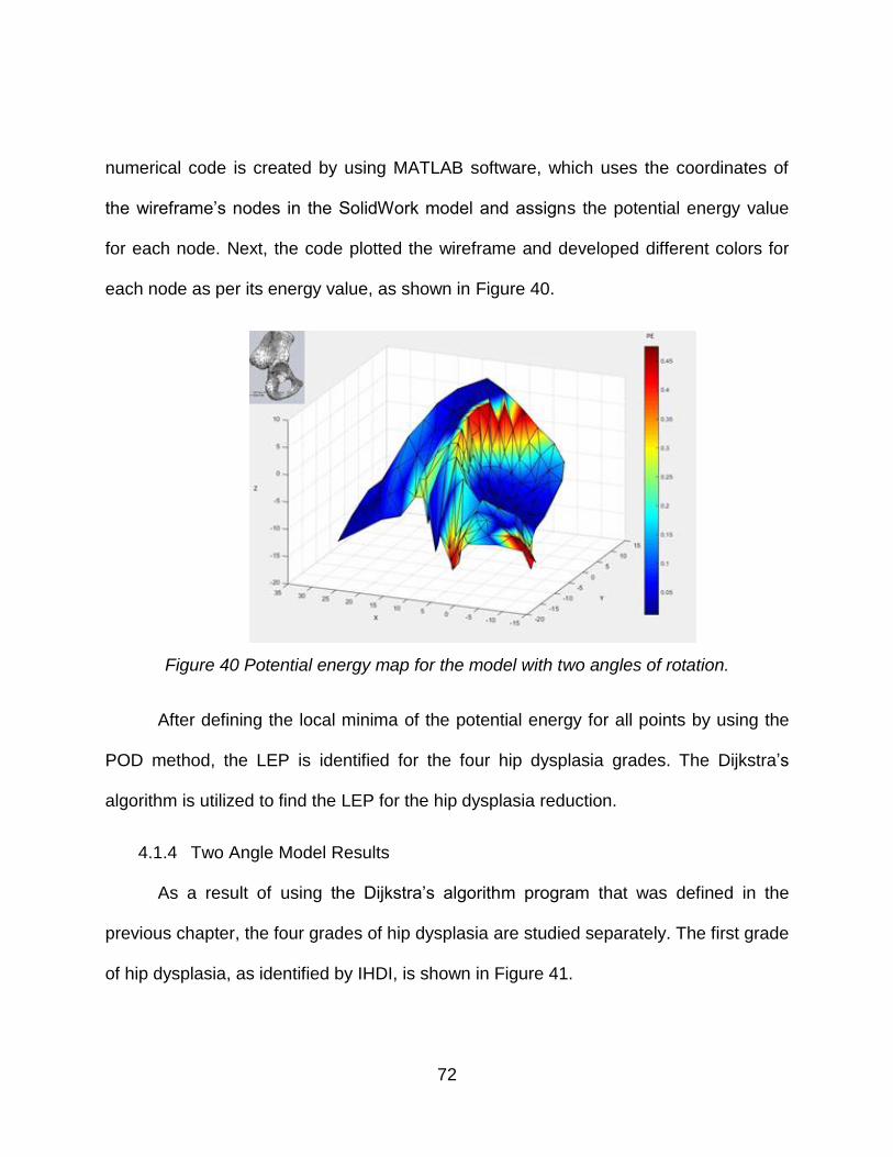
72
numerical code is created by using MATLAB software, which uses the coordinates of
the wireframe’s nodes in the SolidWork model and assigns the potential energy value
for each node. Next, the code plotted the wireframe and developed different colors for
each node as per its energy value, as shown in Figure 40.
Figure 40 Potential energy map for the model with two angles of rotation.
After defining the local minima of the potential energy for all points by using the
POD method, the LEP is identified for the four hip dysplasia grades. The Dijkstra’s
algorithm is utilized to find the LEP for the hip dysplasia reduction.
4.1.4 Two Angle Model Results
As a result of using the Dijkstra’s algorithm program that was defined in the
previous chapter, the four grades of hip dysplasia are studied separately. The first grade
of hip dysplasia, as identified by IHDI, is shown in Figure 41.

73
Figure 41 International Hip Dysplasia Institute classification of Grade I.
As seen in the figure, the source point is located just above the natural position
of the femoral head. After identifying the source point and the target point, the result of
the code is the LEP of hip dysplasia reduction and is shown in Figure 42. The hip
dysplasia reduction path should be through the points identified in the picture while
keeping the femur orientation at a flexion angle of 70 degrees and abduction angle of 90
degrees for the LEP.

74
Figure 42 Grade I: Hip Dysplasia reduction path.
For grade II, the IHDI defined the femoral head as being located underneath the
acetabulum rim, as depicted in Figure 43. After identifying the source point and the
target point, the LEP is created from the Dijkstra’s algorithm, as shown in Figure 44.
The hip dysplasia reduction path should be through the points where identified in the
picture while keeping the femur orientation at a flexion angle of 70 degrees and an
abduction angle of 90 degrees.

75
Figure 43 International Hip Dysplasia Institute classification of grade II.
Figure 44 Grade II: Hip Dysplasia reduction path.
For grade III, the IHDI explained that the femoral head is located on the
acetabulum rim, as displayed in Figure 45. After identifying the source point and the
target point, the resulted LEP is shown in Figure 46. However, the femur is flexed at 70

76
degrees with 54 degrees of abduction. Then the femur is abducted to 90 degrees at the
end of the LEP.
Figure 45 International Hip Dysplasia Institute classification of grade III.
Figure 46 Grade III: Hip Dysplasia reduction path.

77
According to IHDI, the femoral head in grade IV is located outside the
acetabulum rim, as shown in Figure 47, where it is in non-equilibrium condition. This
grade is considered to be the most severe hip dysplasia grade. Moreover, it is quite a
big challenge for the physician to treat babies with this kind of dislocation. In this
research, the main goal is to identify the path of all grades—the most significant of
which is grade IV.
Figure 47 International Hip Dysplasia Institute classification of grade IV.
Therefore, the source point and the target point are identified for grade IV, which
are node number 131 and node number 75, as defined in Table 3 above. The resulted
path has the route of the femoral head moving along specific points with a specific
femur orientation. As listed in Table 6, the femur should be flexed at 70 degrees during
the reduction, but the abduction angle has changed. Furthermore, the femoral head is
moved from the source point to the acetabulum rim by increasing the abduction angle
gradually to 60 degrees. Following, the femur is moved along the rim by increasing the
abduction angle gradually until it reaches the acetabulum notch with an abduction angle
of 90 degrees. Finally, the femur is passed the acetabulum notch to reach the

78
acetabulum center with flexion angle of 70 degrees and abduction angle of 90 degrees.
Figure 48 shows the reduction path of Grade IV.
Table 6 Grade IV hip dysplasia reduction path and orientation.
# Point No. Flexion Abduction
1 131 70 54
2 132 70 42
3 123 70 54
4 122 70 60
5 112 70 60
6 111 70 66
7 95 70 72
8 92 70 78
9 17 70 90
10 38 70 90
11 58 70 90
12 57 70 90
13 61 70 90
14 75 70 90

79
Figure 48 Grade IV: Hip dysplasia reduction path.
To provide accuracy for the hip dysplasia reduction path, the third femur
orientation angle (hip rotation angle) is added to the study. In the hip dysplasia
treatment using the Pavlik Harness, the femur is free to rotate in three angles as
specified previously. However, in the previous model that has only two angles of
rotation, the model was studied and analyzed for the verification of the proposed
method. Therefore, the third rotation angle is added to examine the reduction of the
femur.
4.2 Three Angle Model
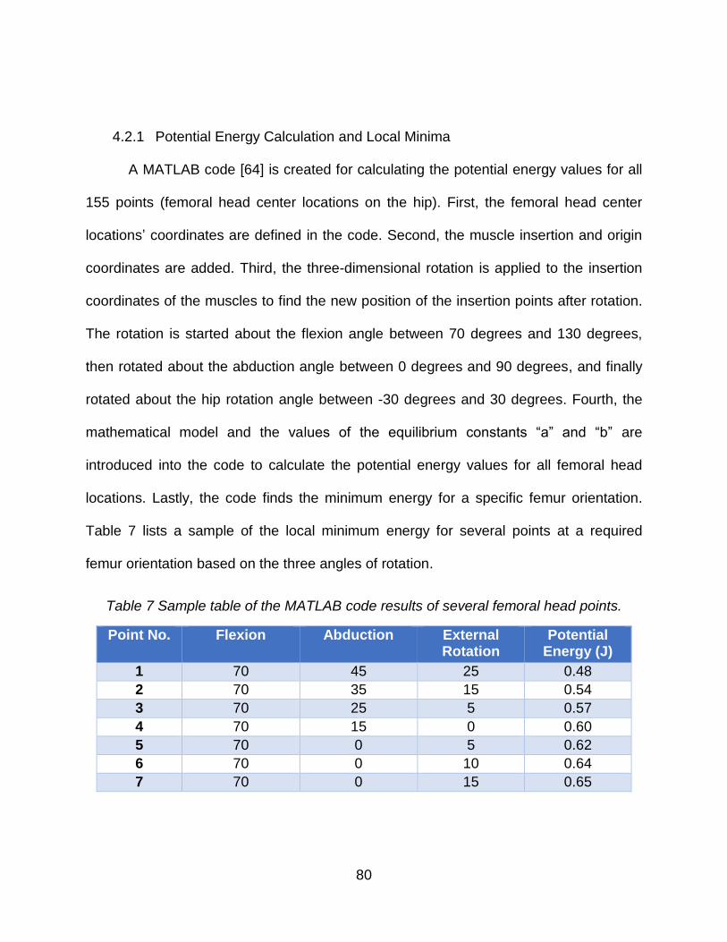
80
4.2.1 Potential Energy Calculation and Local Minima
A MATLAB code [64] is created for calculating the potential energy values for all
155 points (femoral head center locations on the hip). First, the femoral head center
locations’ coordinates are defined in the code. Second, the muscle insertion and origin
coordinates are added. Third, the three-dimensional rotation is applied to the insertion
coordinates of the muscles to find the new position of the insertion points after rotation.
The rotation is started about the flexion angle between 70 degrees and 130 degrees,
then rotated about the abduction angle between 0 degrees and 90 degrees, and finally
rotated about the hip rotation angle between -30 degrees and 30 degrees. Fourth, the
mathematical model and the values of the equilibrium constants “a” and “b” are
introduced into the code to calculate the potential energy values for all femoral head
locations. Lastly, the code finds the minimum energy for a specific femur orientation.
Table 7 lists a sample of the local minimum energy for several points at a required
femur orientation based on the three angles of rotation.
Table 7 Sample table of the MATLAB code results of several femoral head points.
Point No. Flexion Abduction External Rotation
Potential Energy (J)
1 70 45 25 0.48
2 70 35 15 0.54
3 70 25 5 0.57
4 70 15 0 0.60
5 70 0 5 0.62
6 70 0 10 0.64
7 70 0 15 0.65
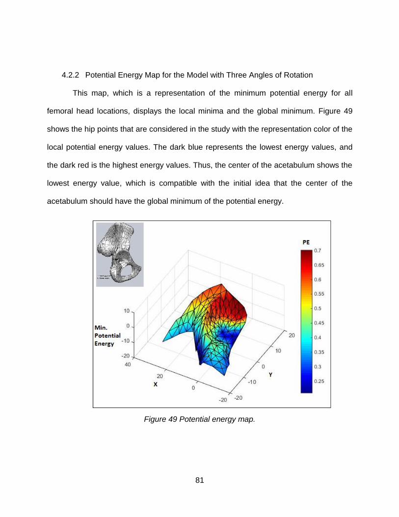
81
4.2.2 Potential Energy Map for the Model with Three Angles of Rotation
This map, which is a representation of the minimum potential energy for all
femoral head locations, displays the local minima and the global minimum. Figure 49
shows the hip points that are considered in the study with the representation color of the
local potential energy values. The dark blue represents the lowest energy values, and
the dark red is the highest energy values. Thus, the center of the acetabulum shows the
lowest energy value, which is compatible with the initial idea that the center of the
acetabulum should have the global minimum of the potential energy.
Figure 49 Potential energy map.

82
4.2.3 Three Angle Model Results
After finding the local minimum of the potential energy for the specified femoral
head locations on the hip, Dijkstra’s algorithm program is used to create the reduction
path for all four hip dysplasia grades.
a. Grade I
Dijkstra’s algorithm is used to find the reduction path with the required femur
orientation, as listed in Table 8. Figure 50 shows the LEP of hip dysplasia reduction for
grade I. The femur should be flexed at 90 degrees during the reduction but abducted
gradually from 40 degrees to 80 degrees with external rotation between 10 and 0
degrees until it reaches the center of the acetabulum.
Table 8 Grade I: required femur orientation for the hip dysplasia reduction.
# Point # Flexion Abduction Hip Rotation
1 66 70 40 10
2 67 70 60 0
3 75 70 80 10

83
Figure 50 Grade I: Hip Dysplasia reduction path with using three angles of rotation.
b. Grade II
Table 9 lists the required femur orientation angles for the reduction. Thus, the
femur should be flexed at an angle of 70 degrees during the reduction and abducted
gradually from 0 degrees to 60 degrees while changing the hip rotation externally
between 0 and 5 degrees during the reduction path. Figure 51 shows the LEP of hip
dysplasia reduction for grade II by using the Dijkstra’s program.
Table 9 Grade II: required femur orientation for the hip dysplasia reduction.
# Point # Flexion Abduction Hip Rotation
1 27 70 0 5
2 47 70 20 0
3 65 70 40 5
4 67 70 60 0
5 75 70 80 10
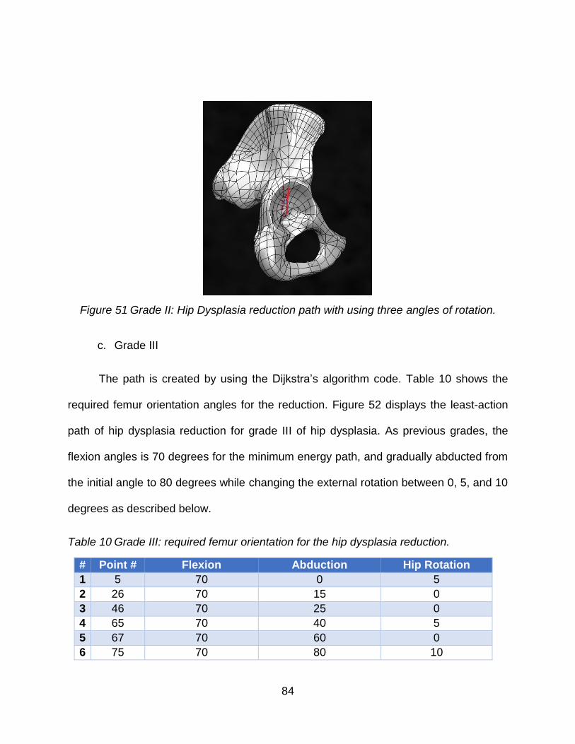
84
Figure 51 Grade II: Hip Dysplasia reduction path with using three angles of rotation.
c. Grade III
The path is created by using the Dijkstra’s algorithm code. Table 10 shows the
required femur orientation angles for the reduction. Figure 52 displays the least-action
path of hip dysplasia reduction for grade III of hip dysplasia. As previous grades, the
flexion angles is 70 degrees for the minimum energy path, and gradually abducted from
the initial angle to 80 degrees while changing the external rotation between 0, 5, and 10
degrees as described below.
Table 10 Grade III: required femur orientation for the hip dysplasia reduction.
# Point # Flexion Abduction Hip Rotation
1 5 70 0 5
2 26 70 15 0
3 46 70 25 0
4 65 70 40 5
5 67 70 60 0
6 75 70 80 10

85
Figure 52 Grade III: Hip Dysplasia reduction path with using three angles of rotation.
d. Grade IV
Two types of analysis are implemented for grade IV. The first analysis determined
the LEP from the starting point of a Grade IV dislocated hip to the acetabulum center
(direct path). The second analysis is implemented to determine the required energy of
the two-stage pathway (indirect path) that follows the modified Hoffman-Daimler result,
which is a path that goes to the intermediate point on the ischium near the acetabular
notch. Furthermore, in each analysis, the effect of the Pectineus is computationally
switched off to evaluate the reduction pathways and to illustrate the changes in the
required energy between the reduction of a model with all muscles intact and one
without the effect of the Pectineus.

86
For the purpose of studying the reduction pathway, the Dijkstra’s algorithm
program is used to find the direct LEP with the presence of all muscles. Table 11 lists
the evaluated LEP with the required femur orientation. The reduction path starts with a
flexed femur at an angle of 70 degrees and continues along the path. The femur is
guided to be abducted at 40 degrees, and then increased gradually to 80 degrees while
changing the hip rotation angle internally from 30 degrees to -30 degrees ending up with
an external rotation of 10 degrees at the center of the acetabulum. The resulting
pathway is shown in Figure 53. Figure 54 shows the potential energy map with the LEP
for this analysis.
Table 11 Grade IV: required femur orientation for the hip dysplasia reduction (Direct path) with the effect of all muscles.
# Point # Flexion Abduction Hip Rotation
1 131 70 40 30
2 124 70 50 30
3 121 70 55 30
4 112 70 55 30
5 111 70 55 30
6 99 75 55 30
7 93 130 70 30
8 19 70 60 -30
9 39 70 60 -30
10 59 70 65 -30
11 60 70 60 -30
12 62 70 70 5
13 75 70 80 10
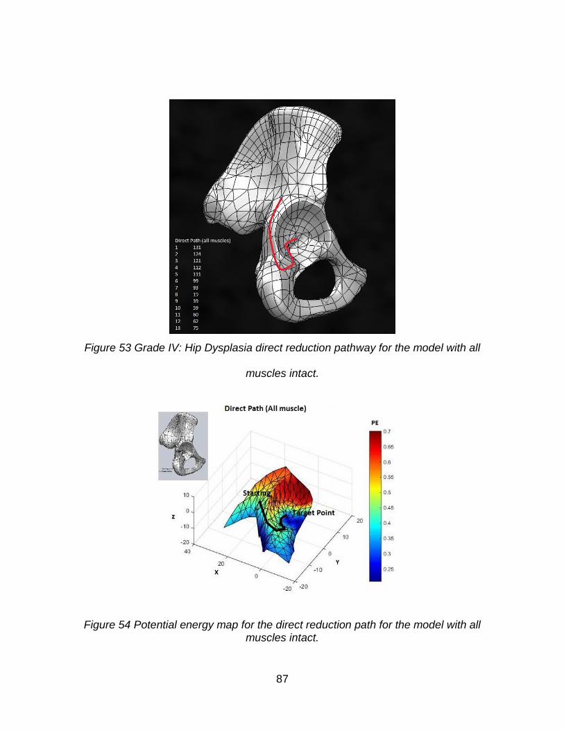
87
Figure 53 Grade IV: Hip Dysplasia direct reduction pathway for the model with all
muscles intact.
Figure 54 Potential energy map for the direct reduction path for the model with all muscles intact.

88
For demonstration purposes, the lower limb bones are scaled down by a scaling
factor of 4:10. Then, at each point on the reduction pathway, the femur is rotated as
determined from the results of the Dijkstra’s algorithm, as shown in Figure 55.

89

90
Figure 55 Grade IV direct reduction path with femur orientation for the model with all muscles.
Table 12 lists the computed direct pathway points with the required femur
orientation angles to achieve the least energy path for the model that does not have the
effect of the Pectineus. Figure 56 shows the resulting pathway that closely followed the
direct pathway proposed by Iwasaki and was documented by Suzuki. To achieve
reduction with the lowest energy, the femur should be flexed at 70 degrees along the
path. However, the abduction angle is changed from 40 to 90 degrees while the hip is

91
rotated internally from 0 degrees to -30 degrees. Figure 57 shows the potential energy
map with the LEP for this analysis.
Table 12 Grade IV: required femur orientation for the hip dysplasia direct reduction of the model without the effect of the Pectineus.
# Point # Flexion Abduction hip rotation
1 131 70 40 0
2 124 70 50 -15
3 122 70 50 -30
4 1 70 50 -30
5 22 70 55 -30
6 43 70 60 -30
7 63 70 70 -30
8 75 70 90 -30
Figure 56 Grade IV: Hip Dysplasia direct reduction path for the model without the effect of the Pectineus.

92
Figure 57 Potential energy map for the direct reduction path for the model without the effect of the Pectineus muscle.
For demonstration purposes, the lower limb bones are scaled down with a
scaling factor of 4:10 and rotated as found from the Dijkstra’s algorithm program to
show the femur orientation during the reduction path. Figure 58 shows different images
which are presenting the required femur orientation for the reduction at each point in the
path.

93
Figure 58 Grade IV direct reduction path with femur orientation for the model without the
effect of the Pectineus.
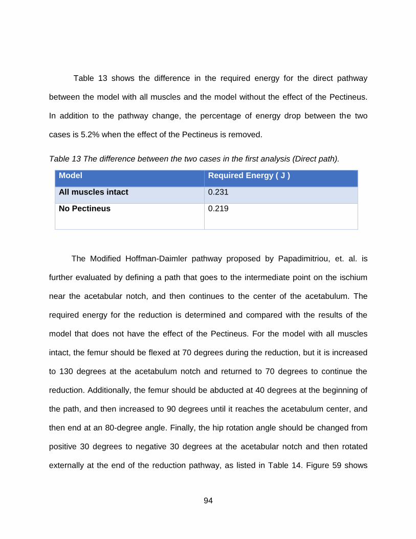
94
Table 13 shows the difference in the required energy for the direct pathway
between the model with all muscles and the model without the effect of the Pectineus.
In addition to the pathway change, the percentage of energy drop between the two
cases is 5.2% when the effect of the Pectineus is removed.
Table 13 The difference between the two cases in the first analysis (Direct path).
Model Required Energy ( J )
All muscles intact 0.231
No Pectineus 0.219
The Modified Hoffman-Daimler pathway proposed by Papadimitriou, et. al. is
further evaluated by defining a path that goes to the intermediate point on the ischium
near the acetabular notch, and then continues to the center of the acetabulum. The
required energy for the reduction is determined and compared with the results of the
model that does not have the effect of the Pectineus. For the model with all muscles
intact, the femur should be flexed at 70 degrees during the reduction, but it is increased
to 130 degrees at the acetabulum notch and returned to 70 degrees to continue the
reduction. Additionally, the femur should be abducted at 40 degrees at the beginning of
the path, and then increased to 90 degrees until it reaches the acetabulum center, and
then end at an 80-degree angle. Finally, the hip rotation angle should be changed from
positive 30 degrees to negative 30 degrees at the acetabular notch and then rotated
externally at the end of the reduction pathway, as listed in Table 14. Figure 59 shows

95
the resulted least energy path for the indirect pathway for the model with all muscles
intact. Figure 60 shows the potential energy map with the LEP for this analysis.
Table 14 Grade IV: required femur orientation for the hip dysplasia indirect reduction pathway of the model with all muscles intact.
# Pt. # Flexion Abduction Hip Rotation
1 131 70 40 30
2 124 70 50 30
3 121 70 55 30
4 112 70 55 30
5 111 70 55 30
6 99 75 55 30
7 93 130 70 30
8 92 130 75 30
9 17 130 90 30
10 16 70 90 -30
11 36 70 90 -30
12 56 70 90 -30
13 74 70 85 5
14 75 70 80 10

96
Figure 59 Grade IV: Hip Dysplasia indirect reduction pathway with the effect of all muscles.
Figure 60 Potential energy map for the indirect reduction path for the model with all muscles intact.

97
As specified previously for the direct reduction path in grade IV, the lower limb
bones are scaled by 4:10. For the indirect pathway of hip dysplasia reduction, the femur
is rotated as specified from the Dijkstra’s algorithm program. Figure 61 shows different
images which present the required femur orientation for the reduction at each point in
the pathway.
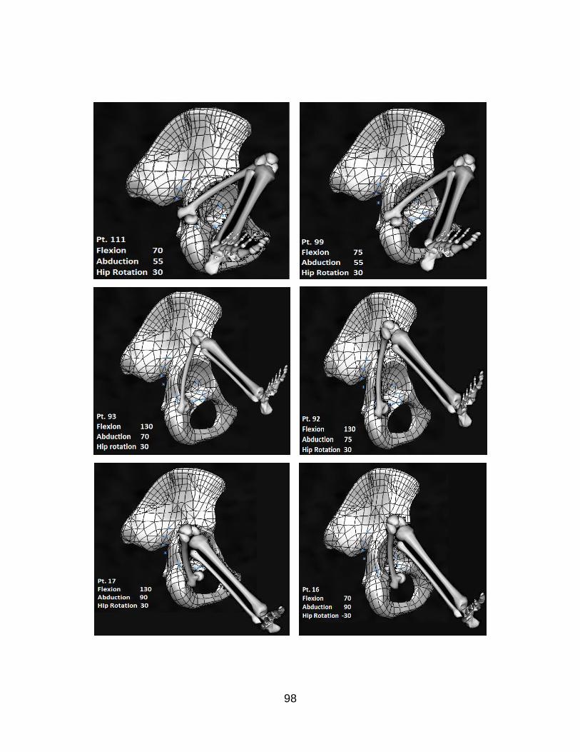
98

99
Figure 61 Grade IV: indirect reduction path with femur orientation for the model with all muscles intact.
Table 15 lists the computed indirect pathway points with the required femur
orientation angles to achieve the least energy path for the model that does not have the
effect of the Pectineus. For the least energy path, the femur should be flexed at 70
degrees along the pathway and abducted from 40 to 90 degrees while the hip is rotated
internally from 0 to -30 degrees. Figure 62 shows the indirect reduction pathway that
goes through the acetabular notch. Figure 63 shows the potential energy map with the
LEP for this analysis.
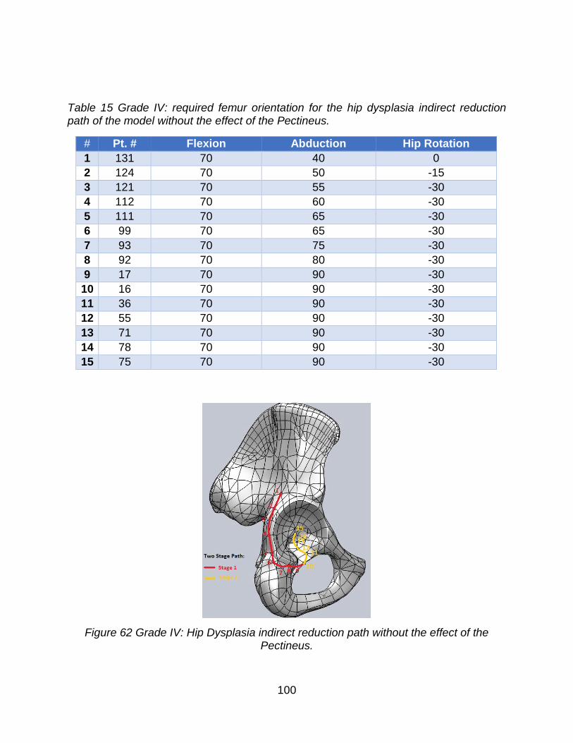
100
Table 15 Grade IV: required femur orientation for the hip dysplasia indirect reduction path of the model without the effect of the Pectineus.
# Pt. # Flexion Abduction Hip Rotation
1 131 70 40 0
2 124 70 50 -15
3 121 70 55 -30
4 112 70 60 -30
5 111 70 65 -30
6 99 70 65 -30
7 93 70 75 -30
8 92 70 80 -30
9 17 70 90 -30
10 16 70 90 -30
11 36 70 90 -30
12 55 70 90 -30
13 71 70 90 -30
14 78 70 90 -30
15 75 70 90 -30
Figure 62 Grade IV: Hip Dysplasia indirect reduction path without the effect of the Pectineus.
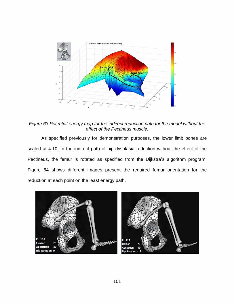
101
Figure 63 Potential energy map for the indirect reduction path for the model without the effect of the Pectineus muscle.
As specified previously for demonstration purposes, the lower limb bones are
scaled at 4:10. In the indirect path of hip dysplasia reduction without the effect of the
Pectineus, the femur is rotated as specified from the Dijkstra’s algorithm program.
Figure 64 shows different images present the required femur orientation for the
reduction at each point on the least energy path.

102
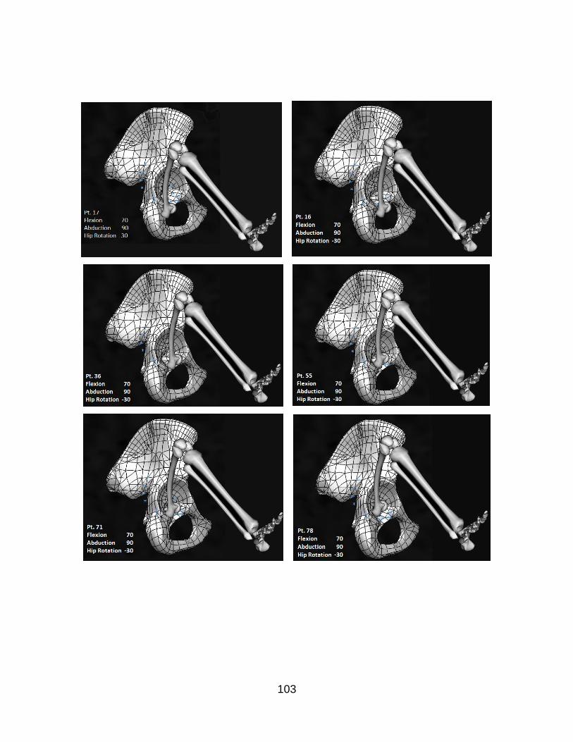
103

104
Figure 64 Grade IV indirect reduction paths with femur orientation for the model without the effect of the Pectineus.
Table 16 shows the difference in the required energy of the indirect path between
the model with all muscles intact and the model without the effect of the Pectineus. The
percentage of energy drop between the two analyses is 9.2% when the effect of the
Pectineus is eliminated.
Table 16 The difference between the third and fourth analysis (indirect path).
Model Required Energy ( J )
All Muscles effect 0.509
No Pectineus 0.462
A fifth calculation is determined by identifying the least energy path from the
dislocated position to the center of the acetabulum without the effect of the Pectineus.
Since this path closely approximated the direct path proposed by Iwasaki, the energy
requirement for this path is determined by all muscles intact. The results indicate that

105
additional energy is required for the femoral head to pass directly over the rim of the
posterior acetabulum when the Pectineus muscle is intact. This supports the findings of
Suzuki that the traction or manual reduction may be needed for the direct reduction of
Grade IV hip dislocation. Table 17 lists the pathway points with the required femur
orientation angles to achieve the least energy path.
Table 18 shows the difference in energy between the second and fifth analysis
that followed the direct pathway proposed by Iwasaki and documented by Suzuki.
Table 17 Least energy path with the required femur orientation for the model with all muscles to follow the proposed pathway by Iwasaki.
# Pt. # Flexion Abduction Hip Rotation
1 131 70 40 30
2 124 70 50 30
3 122 70 50 30
4 1 70 45 25
5 22 70 50 25
6 43 70 55 15
7 63 70 60 5
8 75 70 80 10
Table 18 The difference between the second and the fifth analysis (Direct pathway).
Model Required Energy ( J )
All Muscles effect 0.241
No Pectineus 0.219

106
CHAPTER 5: DISCUSSION AND CONCLUSION
The developed method in this dissertation identifies the least energy path
endorsing the clinical observations of reduction for the four grades of hip dysplasia.
There were several analyses conducted for the severe hip dislocation (Grade IV).
Generally, two different pathways of reduction were considered. The first pathway is the
direct path that starts from the dislocated location to the center of the acetabulum. The
second pathway is the two-stage path that is considered the indirect pathway, which
initially starts from the dislocated location to a point proximal to the ischial tuberosity
and then proceeds to enter the acetabulum from an inferior position. Furthermore,
eliminating the effect of the Pectineus, by numerically switching it off, has demonstrated
a major influence on the required energy for the reduction of Grade IV.
In the first analysis of Grade IV that has the effect of all considered adductor
muscles (Pectineus, Adductor Brevis, Adductor Longus, Adductor Magnus, and
Gracilis), the resulted pathway of least energy closely approximated the indirect
pathway proposed by Papadimitriou, et al [29]. With the studied method, the femoral
head enters the acetabulum at the posterior margin of the lunate articular surface
instead of through the center of the acetabular notch as described in the Modified
Hoffman-Daimler method. Eliminating the effect of the Pectineus in the second analysis
changed the pathway to closely follow the direct pathway proposed by Iwasaki and
documented by Suzuki [22, 21]. This model also demonstrated that eliminating the force
of the Pectineus muscle decreases the energy required for reduction.
5.1 Discussion

107
For the purpose of studying the pathway that was described by the Modified
Hoffman-Daimler method, the computational model was forced to follow a path that
goes through a point proximal to the ischial tuberosity. In this type of study, the resulted
pathways in the two proposed models (the all muscles intact model and the model with
the Pectineus released) successfully followed the pathway of Modified Hoffman-
Daimler, and the effect of eliminating the Pectineus gave the same conclusion of
lowering the required power for the hip reduction.
In the last analysis, the direct pathway of the model with the effect of all muscles
intact was forced to follow the Iwasaki pathway. The femoral head initially shifts to the
posterior part of the acetabulum, slides directly over the acetabular rim, and finally
slides into the acetabulum. The amount of energy required for this reduction path was
higher than the initial one that closely followed the Papadimitriou two-stage result, and
even higher than the one proposed by Iwasaki.
The reduction of all hip dysplasia grades was successfully achieved by applying
the developed method that is based on the principle of stationary potential energy. This
method leads to the identification of a least energy path. Several computer codes were
developed for implementing this study by starting with the collision detection algorithm
that used the three dimensional SolidWorks model of a 10-week-old female infant to find
the femoral head location centers’ coordinates. Next, the muscle mechanics was
introduced by using the non-linear constitutive Fung model that was defined as Hill-type
5.2 Conclusion
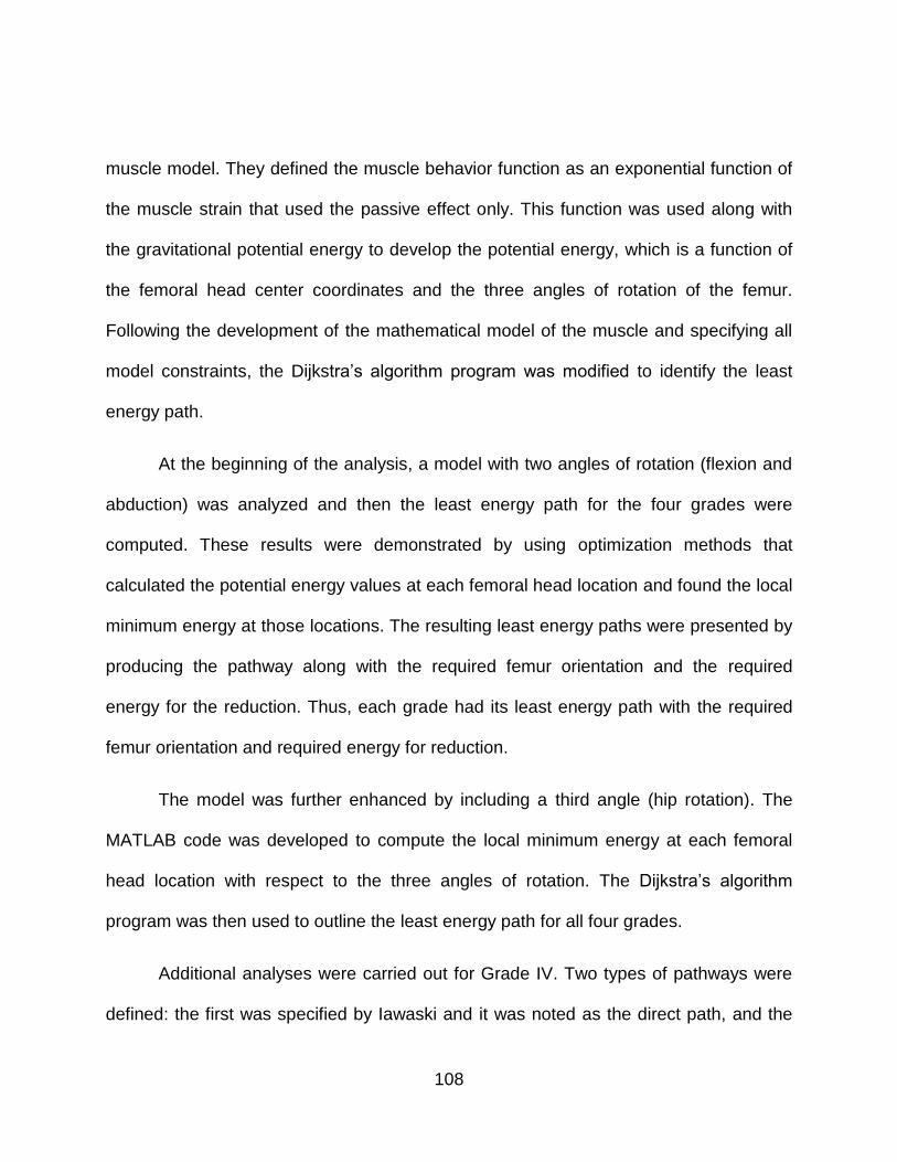
108
muscle model. They defined the muscle behavior function as an exponential function of
the muscle strain that used the passive effect only. This function was used along with
the gravitational potential energy to develop the potential energy, which is a function of
the femoral head center coordinates and the three angles of rotation of the femur.
Following the development of the mathematical model of the muscle and specifying all
model constraints, the Dijkstra’s algorithm program was modified to identify the least
energy path.
At the beginning of the analysis, a model with two angles of rotation (flexion and
abduction) was analyzed and then the least energy path for the four grades were
computed. These results were demonstrated by using optimization methods that
calculated the potential energy values at each femoral head location and found the local
minimum energy at those locations. The resulting least energy paths were presented by
producing the pathway along with the required femur orientation and the required
energy for the reduction. Thus, each grade had its least energy path with the required
femur orientation and required energy for reduction.
The model was further enhanced by including a third angle (hip rotation). The
MATLAB code was developed to compute the local minimum energy at each femoral
head location with respect to the three angles of rotation. The Dijkstra’s algorithm
program was then used to outline the least energy path for all four grades.
Additional analyses were carried out for Grade IV. Two types of pathways were
defined: the first was specified by Iawaski and it was noted as the direct path, and the

109
second was defined from the result of the Modified Hoffman-Daimler pathway that was
an indirect path. The direct pathway was started from the dislocated position of the hip
and ended at the center of the acetabulum, while the indirect pathway followed a path
that entered the acetabulum through the acetabular notch. For both analyses, the effect
of the Pectineus was computationally switched off to compare the required energy for
the reduction. Hence, the findings of this study suggest that release of the Pectineus
muscle may also be considered to facilitate the hip reduction in Grade IV dislocations.
In conclusion, the developed biomechanical computational method is consistent
with the clinical observations stated in the literature, especially the Iwasaki result for the
direct reduction and the Modified Hoffman-Daimler result for the indirect reduction. It
could theoretically provide physicians resources to modify the existing treatment
methods and may lead to new visions of non-surgical management of developmental
dysplasia of the hip.
The work developed in this research improves the prospects of the hip dysplasia
treatment. Furthermore, the results of the developed least energy method will change
the thoughts on hip dysplasia treatments.
It is important to mention that the functionality and design of the harness have
not been modified in more than half a century. The developed mathematical model and
the principle of the stationary potential energy will not only optimize the harness use, but
it will also lead to future development of a new harness. A synthesized harness through
5.3 Future Work

110
the use of inverse methods could be very promising for treating hip dysplasia, especially
for grade IV. The synthesized harness can be a modification of any existing treatment
method by using the computed least energy path along with the required femur
orientation. For instance, the Pavlik Harness’s straps are used to fix the femur in
different orientations at different locations during the reduction. The straps’ setups were
identified as explained in the literature. However, by using the developed method along
with the proven least energy path, the straps with their configuration could be modified
to achieve hip dysplasia reduction as per the achievements of this study.

111
APPENDIX A: COLLISION DETECTION ALGORITHM

112
Appendix A introduced the Collision detection algorithm routine. It is used to
finding the coordinates of the femoral head center when the head is in contact with the
pelvis surface.
Sub FindCenters()
Dim source As Worksheet
Dim destination As Worksheet
Set source = Sheets("Input")
Set centers = Sheets("FHeadCenters")
Const nump = 78 'number of points in the acetabulum
Const r = 7
Const fapp = 30 '% of aproach for each iteration
Dim i, j, L As Integer
Dim D, Min, Min2, magV, magVV, AA(2, nump - 1) As Double
Dim VV(2, nump - 1), V(2), B(2, nump - 1), A(2, nump - 1), CC(2, nump - 1), CCC(2) As Double
Dim M, c As Variant
c = Array(-0.36, -10.05, 17.8)
For i = 0 To nump - 1
B(0, i) = source.Cells(i + 2, 2)
B(1, i) = source.Cells(i + 2, 3)
B(2, i) = source.Cells(i + 2, 4)
Next i
Count2 = 0
For L = 0 To nump - 1
'Calculate the vector of direction of displacement
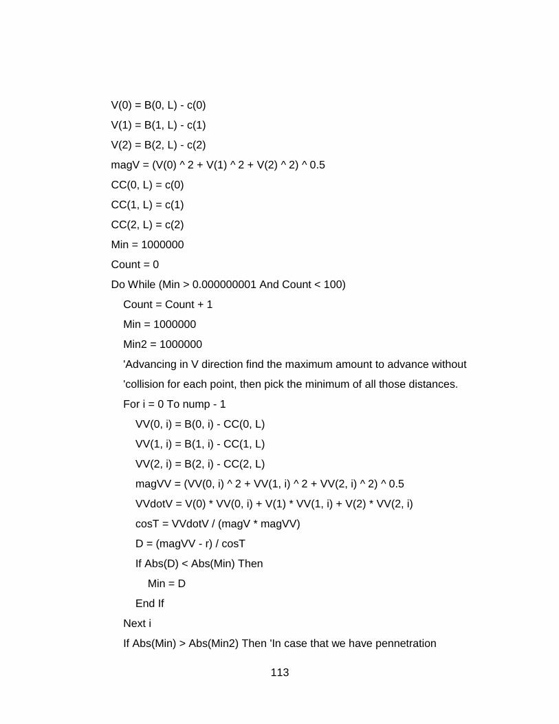
113
V(0) = B(0, L) - c(0)
V(1) = B(1, L) - c(1)
V(2) = B(2, L) - c(2)
magV = (V(0) ^ 2 + V(1) ^ 2 + V(2) ^ 2) ^ 0.5
CC(0, L) = c(0)
CC(1, L) = c(1)
CC(2, L) = c(2)
Min = 1000000
Count = 0
Do While (Min > 0.000000001 And Count < 100)
Count = Count + 1
Min = 1000000
Min2 = 1000000
'Advancing in V direction find the maximum amount to advance without
'collision for each point, then pick the minimum of all those distances.
For i = 0 To nump - 1
VV(0, i) = B(0, i) - CC(0, L)
VV(1, i) = B(1, i) - CC(1, L)
VV(2, i) = B(2, i) - CC(2, L)
magVV = (VV(0, i) ^ 2 + VV(1, i) ^ 2 + VV(2, i) ^ 2) ^ 0.5
VVdotV = V(0) * VV(0, i) + V(1) * VV(1, i) + V(2) * VV(2, i)
cosT = VVdotV / (magV * magVV)
D = (magVV - r) / cosT
If Abs(D) < Abs(Min) Then
Min = D
End If
Next i
If Abs(Min) > Abs(Min2) Then 'In case that we have pennetration
114
Min = -Min
End If
Min2 = Abs(Min)
CC(0, L) = fapp / 100 * V(0) * Min / magV + CC(0, L)
CC(1, L) = fapp / 100 * V(1) * Min / magV + CC(1, L)
CC(2, L) = fapp / 100 * V(2) * Min / magV + CC(2, L)
CCC(0) = CC(0, L)
CCC(1) = CC(1, L)
CCC(2) = CC(2, L)
Loop
centers.Cells(L + 3, 2).Value = CC(0, L)
centers.Cells(L + 3, 3).Value = CC(1, L)
centers.Cells(L + 3, 4).Value = CC(2, L)
If Count > Count2 Then
Count2 = Count
End If
If 1 Then 'Just to check distances
'Calculate all the possible points of contact
For i = 0 To nump - 1
VV(0, i) = B(0, i) - CC(0, L)
VV(1, i) = B(1, i) - CC(1, L)
VV(2, i) = B(2, i) - CC(2, L)
magVV = (VV(0, i) ^ 2 + VV(1, i) ^ 2 + VV(2, i) ^ 2) ^ 0.5
A(0, i) = VV(0, i) * r / magVV + CC(0, L)
A(1, i) = VV(1, i) * r / magVV + CC(1, L)
A(2, i) = VV(2, i) * r / magVV + CC(2, L)
Next i
Min = 1000000
115
For i = 0 To nump - 1
For j = 0 To nump - 1
D = (A(0, i) - B(0, j)) ^ 2 + (A(1, i) - B(1, j)) ^ 2 + (A(2, i) - B(2, j)) ^ 2
If D < Min Then
Min = D
Anode = i
Bnode = j
End If
Next j
Next i
Min = Min ^ 0.5
centers.Cells(L + 3, 9).Value = Min
centers.Cells(L + 3, 11).Value = Anode
centers.Cells(L + 3, 12).Value = Bnode
End If
Next L
centers.Cells(2, 7).Value = Count2
End Sub

116
APPENDIX B: GENETIC ALGORITHM

117
Const PopulationSize As Integer = 100
Const MatingPop As Double = 0.2 'Only the best 20% mates and the best mutation
Dim MaxGenerations, BestPop, posBestMutated As Integer
Dim MutationRate As Double
Dim x, Y, Z As Double
Dim CurrentGeneration(1 To PopulationSize) As Chromosome
Dim Offspring(1 To PopulationSize) As Chromosome
Dim Generation As Integer
Dim SumFitnessScores As Double
Private Sub ShowProgressCheckBox_Click()
End Sub
Private Sub Evolve_Click()
Dim i, j As Integer
Application.ScreenUpdating = ShowProgressCheckBox.Value
Randomize
MaxGenerations = Worksheets("Genetic").Range("MaxGenerations")
MutationRate = Worksheets("Genetic").Range("MutationRate")
BestPop = CInt(MatingPop * PopulationSize)
i = Worksheets("Genetic").Cells(3, 7) 'Starting point in X,Y and Z so you can continue calculating later
Dim a As Boolean
a = IsEmpty(Worksheets("results").Cells(i + 1, 1))
Do While (Not (IsEmpty(Worksheets("results").Cells(i + 1, 1))))
Worksheets("Genetic").Cells(3, 7) = i 'Starting point modified automatically
Appendix B1: Genetic Algorithm Code:

118
x = Worksheets("results").Cells(i + 1, 1)
Y = Worksheets("results").Cells(i + 1, 2)
Z = Worksheets("results").Cells(i + 1, 3)
For j = 1 To PopulationSize
Set CurrentGeneration(j) = New Chromosome
Set Offspring(j) = New Chromosome
CurrentGeneration(j).x = x
CurrentGeneration(j).Y = Y
CurrentGeneration(j).Z = Z
CurrentGeneration(j).MutationRate = MutationRate
Next
DoGeneticAlgorithm
Application.ScreenUpdating = True
Application.ActiveWorkbook.Save
With Worksheets("results")
.Cells(1 + i, 4) = Worksheets("Genetic").Cells(3, 2)
.Cells(1 + i, 5) = Worksheets("Genetic").Cells(3, 3)
.Cells(1 + i, 6) = Worksheets("Genetic").Cells(3, 4)
End With
i = i + 1
Loop
End Sub
Public Sub DoGeneticAlgorithm()
Dim i As Integer
Dim mom As Integer
Dim dad As Integer
'Dim m As Integer

119
Generation = 0
posBestMutated = -1
Do While (Generation <= MaxGenerations)
EvaluteFitness
DisplayResults 'Here we also arrange the points in Energy order
posBestMutated = -1 'Just to initialize it and use -1 as reference to know there is no mutation
For i = 1 To BestPop
Offspring(i).Copy CurrentGeneration(Worksheets("Genetic").Cells(i + 2, 1))
Next
For i = BestPop + 1 To PopulationSize
mom = SelectChromosome
dad = SelectChromosome
Offspring(i).Mate CurrentGeneration(mom), CurrentGeneration(dad)
If Offspring(i).Bmutated = True Then 'If a mutation happen during mate
Offspring(i).EvaluateE
If posBestMutated = -1 Then
posBestMutated = i
Else
If Offspring(i).E <= Offspring(posBestMutated).E Then
posBestMutated = i
Else
Offspring(i).Bmutated = False
End If
End If
End If
Next

120
For i = 1 To PopulationSize
CurrentGeneration(i).Copy Offspring(i)
Next
Generation = Generation + 1
Loop
End Sub
Public Sub EvaluteFitness()
Dim i, pos As Integer
Dim MinE As Double
Dim MaxE As Double
CurrentGeneration(1).EvaluateE
MinE = CurrentGeneration(1).E
MaxE = CurrentGeneration(1).E
pos = 1
For i = 2 To PopulationSize
CurrentGeneration(i).EvaluateE
If CurrentGeneration(i).E > MaxE Then
MaxE = CurrentGeneration(i).E
End If
If CurrentGeneration(i).E < MinE Then
MinE = CurrentGeneration(i).E
End If
Next
SumFitnessScores = 0
For i = 1 To PopulationSize
CurrentGeneration(i).FitnessScore = 1 - _
(CurrentGeneration(i).E - MinE) / (MaxE - MinE)

121
SumFitnessScores = SumFitnessScores + CurrentGeneration(i).FitnessScore
Next
End Sub
Public Function SelectChromosome() As Integer
SelectChromosome = CInt(Rnd * (MatingPop * PopulationSize + (1))) + 1 'The (1)is to include also the best mutation
End Function
Public Sub DisplayResults()
Dim i As Integer
Dim r As Integer
Dim found As Boolean
r = 3
For i = 1 To PopulationSize
With Worksheets("Genetic")
.Cells(r, 1) = i
.Cells(r, 2) = CurrentGeneration(i).Ab
.Cells(r, 3) = CurrentGeneration(i).Fl
.Cells(r, 4) = CurrentGeneration(i).E
.Cells(r, 5) = CurrentGeneration(i).mutant
End With
r = r + 1
Next
' Sort the results:
Range("A2", Range("E" & Rows.Count).End(xlUp).Address).Sort Key1:=Range("D3"), _
Order1:=xlAscending, Header:=xlYes

122
Worksheets("Genetic").Range("Generation") = Generation 'Shows in which generation we are
If posBestMutated <> -1 Then
' Put the mutated Chromosome at the end of the list of the best Population if it was not in the best population
found = False
'Plot best mutated
Worksheets("Genetic").Cells(2, 15) = CurrentGeneration(posBestMutated).Ab
Worksheets("Genetic").Cells(2, 16) = CurrentGeneration(posBestMutated).Fl
For i = 1 To BestPop
If Worksheets("Genetic").Cells(2 + i, 1) = posBestMutated Then
Worksheets("Genetic").Cells(2 + i, 5) = "Best Mutant" 'this line should not be necessary
found = True
Exit For
End If
Next
If found = False Then
With Worksheets("Genetic")
.Cells(BestPop + 3, 1) = posBestMutated
.Cells(BestPop + 3, 2) = CurrentGeneration(posBestMutated).Ab
.Cells(BestPop + 3, 3) = CurrentGeneration(posBestMutated).Fl
.Cells(BestPop + 3, 4) = CurrentGeneration(posBestMutated).E
.Cells(BestPop + 3, 5) = "Best Mutant"
End With
End If
End If
End Sub

123
Public Ab As Double
Public Fl As Double
Public E As Double
Public x As Double
Public Y As Double
Public Z As Double
Public Bmutated As Boolean 'For the best mutant
Public mutant As Boolean 'For sons of one of the best mutanted
Public MaxAb As Double
Public MinAb As Double
Public MaxFl As Double
Public MinFl As Double
Public MutationRate As Double
Public FitnessScore As Double
Private Sub Class_Initialize()
MutationRate = Worksheets("Genetic").Cells(2, 7)
Bmutated = False
mutant = False
MaxAb = 90 * Pi / 180
MinAb = 6 * Pi / 180
MaxFl = 132 * Pi / 180
MinFl = 70 * Pi / 180
Ab = (MaxAb - MinAb - 1) * Rnd + MinAb
Fl = (MaxFl - MinFl - 1) * Rnd + MinFl
EvaluateE
Appendix B2: The Chromosome:

124
End Sub
Public Sub EvaluateE()
E =
End Sub
Public Sub Mutate()
Dim num As Double
Const both = 0.15 'Intersecting range will vary both parameters, not 1
Bmutated = False
num = Rnd
If (num < MutationRate) Then
Bmutated = True 'I asume will be the best mutated this will change after the mate
num = Rnd
If num < (1 - both) Then
Ab = (MaxAb - MinAb - 1) * Rnd + MinAb
End If
If num > both Then
Fl = (MaxFl - MinFl - 1) * Rnd + MinFl
End If
End If
End Sub
Public Sub Mate(mom As Chromosome, dad As Chromosome)
Dim num As Double
num = Rnd
Ab = (1 - num) * mom.Ab + num * dad.Ab
num = Rnd
Fl = (1 - num) * mom.Fl + num * dad.Fl

125
' Mutate the result
Mutate
' To show if one of the parents were the best mutated of the parents generation
If mom.Bmutated = True Or dad.Bmutated = True Then
mutant = True
Else
mutant = False
End If
End Sub
Public Sub Copy(dup As Chromosome)
Ab = dup.Ab
Fl = dup.Fl
E = dup.E
MaxAb = dup.MaxAb
MinAb = dup.MinAb
MaxFl = dup.MaxFl
MinFl = dup.MinFl
MutationRate = dup.MutationRate
FitnessScore = dup.FitnessScore
mutant = dup.mutant
Bmutated = dup.Bmutated
End Sub

126
LIST OF REFERENCES
1. Ortolani, M., Congenital hip dysplasia in the light of early and very early
diagnosis. Clinical Orthopaedics And Related Research, 1976(119): p. 6-10.
2. Seringe, R., J.C. Bonnet and E. Katti, Pathogeny and natural history of
congenital dislocation of the hip. Orthopaedics & Traumatology: Surgery &
Research, 2014. 100(1): p. 59-67.
3. Barlow, T.G., EARLY DIAGNOSIS AND TREATMENT OF CONGENITAL
DISLOCATION OF THE HIP. Journal of Bone & Joint Surgery, British Volume,
1962. 44-B(2): p. 292-301.
4. Weinstein, S.L., S.J. Mubarak and D.R. Wenger, Developmental Hip Dysplasia
and Dislocation. Part I. Vol. 85. 2003. 1824-1832.
5. Ardila, O.J., Eduardo A. Divo, Faissal A. Moslehy, George T. Rab, Alain J.
Kassab, and Charles T. Price, Mechanics of hip dysplasia reductions in infants
using the Pavlik harness: A physics-based computational model. Journal of
Biomechanics, 2013. 46(9): p. 1501-1507.
6. Price, C., Castanedo, P., Clarke, N., Cundy, P., Herarro-Soto, J., Hosalkar, H.,
Kasser, J., Mubarak, S., Wedege, J., and Narayanan, U., Reliability of a New
Radiographic Classification of Developmental Hip Dysplasia. Journal of Child
Orthopaedics, 2011. 5(1): p. 1-35.
7. Stuart L. Weinstein, M., Scott J. Mubarak, MD, AND Dennis R. Wenger, MD,
Developmental Hip Dysplasia and Dislocation, ed. S.L. Weinstein, S.J. Mubarak
and D.R. Wenger. Vol. 85. 2003. 2024-2035.

127
8. Kitoh, H., M. Kawasumi and N. Ishiguro, Predictive Factors for Unsuccessful
Treatment of Developmental Dysplasia of the Hip by the Pavlik Harness.
JOURNAL OF PEDIATRIC ORTHOPAEDICS, 2009. 29(6): p. 552-557.
9. Huayamave, V., C. Rose, S. Serra, B. Jones, E. Divo, F. Moslehy, A.J. Kassab
and C.T. Price, A patient-specific model of the biomechanics of hip reduction for
neonatal Developmental Dysplasia of the Hip: Investigation of strategies for low
to severe grades of Developmental Dysplasia of the Hip. Journal of
Biomechanics, 2015.
10. Tibrewal, S., V. Gulati and M. Ramachandran, The Pavlik method: a systematic
review of current concepts.
11. Pavlik, A., The functional method of treatment using a harness with stirrups as
the primary method of conservative therapy for infants with congenital dislocation
of the hip. 1957. Clinical Orthopaedics And Related Research, 1992(281): p. 4-
10.
12. Mubarak, S.J. and V. Bialik, Pavlik: The man and his method.
13. Pavlik, A., Stirrups as an aid in the treatment of congenital dysplasias of the hip
in children. By Arnold Pavlik, 1950. Journal Of Pediatric Orthopedics, 1989. 9(2):
p. 157-159.
14. Bin, K., J.M. Laville and F. Salmeron, Developmental dysplasia of the hip in
neonates: Evolution of acetabular dysplasia after hip stabilization by brief Pavlik
harness treatment. Orthopaedics & Traumatology: Surgery & Research, 2014.
100(4): p. 357-361.

128
15. Mubarak, S., S. Garfin, R. Vance, B. McKinnon and D. Sutherland, PITFALLS IN
THE USE OF THE PAVLIK HARNESS FOR TREATMENT OF CONGENITAL
DYSPLASIA SUB LUXATION AND DISLOCATION OF THE HIP. Journal of
Bone and Joint Surgery American Volume, 1981. 63(8): p. 1239-1248.
16. Grill, F., H. Bensahel, J. Canadell, P. Dungl, T. Matasovic and T. Vizkelety, THE
PAVLIK HARNESS IN THE TREATMENT OF CONGENITAL DISLOCATING
HIP REPORT ON A MULTICENTER STUDY OF THE EUROPEAN PEDIATRIC
ORTHOPEDIC SOCIETY. JOURNAL OF PEDIATRIC ORTHOPAEDICS, 1988.
8(1): p. 1-8.
17. Guille, J.T., P.D. Pizzutillo and G.D. MacEwen, Development dysplasia of the hip
from birth to six months. The Journal Of The American Academy Of Orthopaedic
Surgeons, 2000. 8(4): p. 232-242.
18. Peled, E., V. Bialik, A. Katzman, M. Eidelman and D. Norman, Treatment of
Graf's ultrasound class III and IV hips using Pavlik's method.
19. Kalamchi, A. and R. Macfarlane, III, THE PAVLIK HARNESS RESULTS IN
PATIENTS OVER 3 MONTHS OF AGE. Journal of Parenteral Science and
Technology, 1982. 2(1): p. 3-8.
20. Atalar, H., U. Sayli, O.Y. Yavuz, I. Uraş and H. Dogruel, Indicators of successful
use of the Pavlik harness in infants with developmental dysplasia of the hip.
International Orthopaedics, 2007. 31(2): p. 145-150.
129
21. Suzuki, S., Reduction of CDH by the Pavlik harness. Spontaneous reduction
observed by ultrasound. The Journal Of Bone And Joint Surgery. British Volume,
1994. 76(3): p. 460-462.
22. Iwasaki, K., TREATMENT OF CONGENITAL DISLOCATION OF THE HIP BY
THE PAVLIK HARNESS MECHANISMS OF REDUCTION AND USAGE. Journal
of Bone and Joint Surgery American Volume, 1983. 65(6): p. 760-767.
23. Viere, R.G., J.G. Birch, J.A. Herring, J.W. Roach and C.E. Johnston, USE OF
THE PAVLIK HARNESS IN CONGENITAL DISLOCATION OF THE HIP AN
ANALYSIS OF FAILURES OF TREATMENT. Journal of Bone and Joint Surgery
American Volume, 1990. 72(2): p. 238-244.
24. Miller, B., Hip Dysplasia. Pediatrics for Parents, 2007. 23(5): p. 12-13.
25. Seidl, T., J. Lohmaier, T. Holker, J. Funk, R. Placzek and H.H. Trouillier,
Reduction of unstable and dislocated hips applying the Tubingen hip flexion
splint? 2012.
26. Bernau, A., [The Tübingen hip flexion splint in the treatment of hip dysplasia].
Zeitschrift Für Orthopädie Und Ihre Grenzgebiete, 1990. 128(4): p. 432-435.
27. Atalar, H., C. Gunay and M. Komurcu, Functional treatment of developmental hip
dysplasia with the Tübingen hip flexion splint. Hip International: The Journal Of
Clinical And Experimental Research On Hip Pathology And Therapy, 2014.
24(3): p. 295-301.
130
28. Wilkinson, A.G., D.A. Sherlock and G.D. Murray, The efficacy of the Pavlik
harness, the Craig splint and the von Rosen splint in the management of
neonatal dysplasia of the hip - A comparative study.
29. Papadimitriou, N.G., A. Papadimitriou, J.E. Christophorides, T.A. Beslikas and
P.K. Panagopoulos, Late-Presenting Developmental Dysplasia of the Hip
Treated with the Modified Hoffmann-Daimler Functional Method. Vol. 89. 2007.
1258-1268.
30. Lewars, E., Computational chemistry [electronic resource] : introduction to the
theory and applications of molecular and quantum mechanics / Errol Lewars.
2010: Dordrecht ; London : Springer, 2010. 2nd ed.
31. Huayamave, V., Ceballos, A, Divo, E, Kassab, A, Barkaszi, S, Seigneur, H,
Barriento, POD-accelerated CFD analysis of wind loads on PV systems, in 10th
International Conference on Heat Transfer, Fluid Mechanics and
Thermodynamics. 2014, International Conference on Heat Transfer, Fluid
Mechanics and Thermodynamics: Florida.
32. Ostrowski, Z., R. Białecki and A. Kassab, Estimation of constant thermal
conductivity by use of Proper Orthogonal Decomposition. Computational
Mechanics, 2005. 37(1): p. 52-59.
33. Quapp, W. and D. Heidrich, Analysis of the concept of minimum energy path on
the potential energy surface of chemically reacting systems. Theoretica chimica
acta, 1984. 66(3-4): p. 245-260.

131
34. Scharfenberg, P., Analysis of critical points on the potential energy surface.
Theoretica chimica acta, 1980. 58(1): p. 73-79.
35. Smidstrup, S., A. Pedersen, K. Stokbro and H. Jónsson, Improved initial guess
for minimum energy path calculations. Journal of Chemical Physics, 2014.
140(21): p. 214106-214101-214106-214106.
36. Schlegel, H.B., Geometry optimization on potential energy surfaces. Modern
Electronic Structure Theory, 1995. 2: p. 459-500.
37. Nichols, J., H. Taylor, P. Schmidt and J. Simons, Walking on potential energy
surfaces. Journal of Chemical Physics, 1990. 92(1): p. 340.
38. Basilevsky, M.V. and A.G. Shamov, The local definition of the Optimum ascent
path on a multi-dimensional potential energy surface and its practical application
for the location of saddle points. Chemical Physics, 1981. 60(3): p. 347-358.
39. Kiryati, N. and G. Szekely, Estimating shortest paths and minimal distances on
digitized three-dimensional surfaces. Pattern Recognition, 1993. 26(11): p. 1623-
1637.
40. Stefanakis, E. and M. Kavouras, On the determination of the optimum path in
space. SPATIAL INFORMATION THEORY, 1995. 988: p. 241-257.
41. Mitchell, J.S., D.M. Mount and C.H. Papadimitriou, The discrete geodesic
problem. SIAM Journal on Computing, 1987. 16(4): p. 647-668.
42. Aleksandrov, L., H. Djidjev, A. Maheshwari and J.R. Sack, An Approximation
Algorithm for Computing Shortest Paths in Weighted 3-d Domains. 2011.

132
43. Kimmel, R. and N. Kiryati, Finding the shortest paths on surfaces by fast global
approximation and precise local refinement.
44. Delp, S.L., F.C. Anderson, A.S. Arnold, P. Loan, A. Habib, C.T. John, E.
Guendelman and D.G. Thelen, OpenSim: Open-Source Software to Create and
Analyze Dynamic Simulations of Movement. Biomedical Engineering, IEEE
Transactions on, 2007. 54(11): p. 1940-1950.
45. Arnold, E., S. Ward, R. Lieber and S. Delp, A Model of the Lower Limb for
Analysis of Human Movement. Annals of Biomedical Engineering, 2010. 38(2): p.
269-279.
46. Huayamave, V., Rose, C., Zwawi, M., Divo, E., Moslehy, F., Kassab, A.J., Price,
C., Mechanics of Hip Dysplasia Reduction in Infants with the Pavlik Harness
using Patient Specific Geometry, in Proceedings of ASME-IMECE 2014. 2014:
Montreal, Canada.
47. The Visible Human Project, Us National Library of Medicine. 1994; Available
from: http://www.nlm.nih.gov/research/visible/.
48. Dostal, W.F. and J.G. Andrews, A three-dimensional biomechanical model of hip
musculature. Journal of Biomechanics, 1981. 14(11): p. 803-812.
49. Wickiewicz, T.L., R.R. Roy, P.L. Powell and V.R. Edgerton, Muscle architecture
of the human lower limb. Clinical Orthopaedics And Related Research, 1983.
179: p. 275-283.
50. Friederich, J.A. and R.A. Brand, Muscle fiber architecture in the human lower
limb. Journal of Biomechanics, 1990. 23(1): p. 91-95.

133
51. Delp, S.L., Surgery simulation: a computer graphics system to analyze and
design musculoskeletal reconstructions of the lower limb. 1990, Stanford
University.
52. Marieb, E.N., Human anatomy & physiology. 1998: Menlo Park, Calif. :
Benjamin/Cummings, c1998.
4th ed.
53. Drake, R.L., Gray's atlas of anatomy. 2015: Philadelphia, PA : Churchill
Livingstone, [2015]
Second edition.
54. Agur, A.M.R., A.F. Dalley and J.C.B. Grant, Grant's atlas of anatomy. [electronic
resource]. 2013: Philadelphia : Wolters Kluwer Health/Lippincott Williams &
Wilkins, c2013.
13th ed.
55. Martins, J.A.C., E.B. Pires, R. Salvado and P.B. Dinis, A numerical model of
passive and active behavior of skeletal muscles. Computer Methods in Applied
Mechanics and Engineering, 1998. 151(3–4): p. 419-433.
56. Thelen, D.G., Adjustment of Muscle Mechanics Model Parameters to Simulate
Dynamic Contractions in Older Adults. Journal of Biomechanical Engineering,
2003. 125(1): p. 70-77.

134
57. Calvo, B., A. Ramirez, A. Alonso, J. Grasa, F. Soteras, R. Osta and M.J. Munoz,
Passive nonlinear elastic behaviour of skeletal muscle: Experimental results and
model formulation. Journal of Biomechanics, 2010. 43(2): p. 318-325.
58. Gajdosik, R.L., Passive extensibility of skeletal muscle: Review of the literature
with clinical implications. Clinical Biomechanics, 2001. 16(2): p. 87-101.
59. Herzog, W., Skeletal muscle mechanics : from mechanisms to function. 2000:
Chichester ; New York : John Wiley & Sons, c2000.
60. Winters, J.M., Hill-based muscle models: a systems engineering perspective, in
In, Winters, J.M. and Woo, S.L-Y. (eds.), Multiple muscle systems: biomechanics
and movement organization, New York, Springer-Verlag, 1990, p. 69-93. 1990: ;.
61. Hill, A.V., First and last experiments in muscle mechanics. 1970: Cambridge
[Eng.], University Press, 1970.
62. Fung, Y.C., Structure and Stress-Strain Relationship of Soft Tissues. American
Zoologist, 1984. 24(1): p. 13-22.
63. Magid, A. and D.J. Law, Myofibrils Bear Most of the Resting Tension in Frog
Skeletal Muscle. 1985, The American Association for the Advancement of
Science. p. 1280.
64. MATLAB and Statistics Toolbox Release 2014b, The MathWorks, Inc. Natick,
Massachusetts, United States.
65. Dijkstra, E.W., A note on two problems in connexion with graphs. Numerische
Mathematik, 1959. 1(1): p. 269-271.