mechanics of advanced composite structures artificial
TRANSCRIPT

Mechanics of Advanced Composite Structures 8 (2021) 245-268
Semnan University
Mechanics of Advanced Composite
Structures
journal homepage: http://MACS.journals.semnan.ac.ir
* Corresponding author. Tel.: +98-9127616631 E-mail address: [email protected]
DOI: 10.22075/MACS.2020.20699.1268 Received 20-06-24; Received in revised form 20-08-08; Accepted 20-12-01 © 2021 Published by Semnan University Press. All rights reserved.
Artificial Intelligence Method for Predicting Mechanical Properties of Sand/Glass Reinforced Polymer: a New Model
M. Heshmatia, S. Hayati a*, S. Javanmiria, M. Javadianb a Department of Mechanical Engineering, Kermanshah University of Technology, Kermanshah, 67156-85420, Iran
b Department of Computer Engineering, Kermanshah University of Technology, Kermanshah, 67156-85420, Iran
K E Y W O R D S
A B S T R A C T
Reinforced polymer
Mechanical properties
A new model
Active learning method
Neural networks
In this paper, the aim is to propose a new model to obtain the mechanical properties of
sand/glass polymeric concrete including modulus of elasticity and the ultimate tensile
stress. The neural network soft computation, support vector machine (SVM), and active
learning method (ALM) that is a fuzzy regression model are all used to construct a simple
and reliable model based on experimental datasets. The experimental data are obtained via
the tensile and bending tests of sand/glass reinforced polymer with different weight
percentages of sand and chopped glass fibers. The extracted results are then used for
training and testing of the neural network models. Two different types of neural networks
including feed-forward neural network (FFNN) and radial basis neural network (RBNN)
are employed for connecting the properties of the sand/glass reinforced polymer to the
properties of the resin and weight percentages of sand and glass fibers. Besides the neural
network models, the SVM and ALM models are applied to the problem. The models are
compared with each other with respect to the statistical indices for both train and test
datasets. Finally, to obtain the properties of the sand/glass reinforced polymer, the most
accurate model is presented as an FFNN model.
1. Introduction
In the last decades, polymeric concrete (PC) has been widely used for new constructions and repairing old constructions due to its good properties, such as rapid setting, high strength, corrosion, and water resistance. Polymer concrete (PC) is fabricated generally by combining the polymers and the fillers. The resin, (e.g. epoxy or polyester) plays the role of a binder instead of cement binders in plain concretes [1]. The unsaturated isophthalic and orthophthalic polyesters can be used as a binder in PC at special conditions such as harsh environments like acid or alkaline media or water [2]. Moreover, epoxy resins are widely used for the manufacturing of polymer concretes due to their suitable mechanical properties and especially their high binding resistance.
Because of the adhesion of the polymeric concrete, repairing both polymer and conventional cement-based concretes are possible. Polymer concrete is an ideal material for underground constructions because of its
neutral chemical structure and water impermeability. Conducted studies about mechanical behaviors of such materials under chemical attack situations certify their performance in such situations [3, 4]. While cement-bound mortars cannot resist to chlorine-based acids and the effects of sulfate, polymer-based mortars show resistance both as repair mortar or coating. Polymer concrete also shows good resistance to water and has a high hydraulic capacity thanks to its smoothness [5]. Their adhesion property is the most important property of these materials as they are widely used to reinforce concrete structures [6-12].
Several research works have been conducted for determining the material characteristics of different types of polymer concrete [13-16]. Abdel-Fattah and El-Hawary [17] conducted experiments to study the flexural behavior of polymer concrete (PC) made with epoxy resin and polyester with varying percentages. The results show that the modulus of rupture and ultimate compressive strain for PC were much higher. Thus, the ductility was improved in
Heshmati et al. / Mechanics of Advanced Composite Structures 8 (2021) 245-268
246
comparison with the ordinary Portland cement concrete. Komendant et al. [18] investigated the effect of testing temperature on the compressive strength as well as the influence of thermal cycling between 23 and 71 0C on the strength and elastic properties of concrete. They observed that the compressive strength of the concrete is reduced by 3–11% at 43 0C and 11–21% at 71 0C. However, only a few articles have been published in the literature which consider the effect of environment conditions on the PC properties. In some other works [19-22] a numerical analysis approach was used to investigate the mechanical properties of concrete.
Since the PC exhibits brittle failure behavior, improving its post-peak stress-strain behavior is an important aspect for the application of PC. Hence, developing better PC systems and also characterizing the fracture properties and flexural strength in terms of constituents are essential for the efficient use of PC [23, 24]. Chopped strand glass fiber has been applied to polymer composites for improving the strength and controlling the cracking [25, 26]. Thus, before being used in practical and industrial applications, the study of their mechanical properties is necessary. To characterize the failure behavior of the polymer composites with respect to the constituents, some attempts have been made for efficient use [27] or optimizing the mechanical properties [28, 29].
However, since these materials are newly developed, the study of their mechanical properties is much necessary before using them in practical and industrial applications. Analytical methods such as numerical homogenization are used to determine composite material properties [30]. The microstructure interpolation method is also applied for multiple length scale structural optimization [31]. In addition, Akbari et al [32] applied a multi-scale method based on the homogenization technique to investigate the influence of microscopic parameters on the macroscopic behavior of polycrystalline materials under different loading configurations. Since there is still no mathematical model to obtain the mechanical properties of PCs in general, most of the research work on the mechanical properties are limited to experimental studies [33-41]. Thus, the only way for estimation of the mechanical properties of a PC is through a time consuming and expensive experimental process.
Therefore, in this study, the artificial intelligence (AI) soft computation modeling based on experimental data is chosen to construct a simple and reliable model for the estimation of mechanical properties of the PCs.
As an example, Shabani and Mazaheri used the artificial neural network models in numerical modeling of nano-sized ceramic particulates reinforced metal matrix composites [42]. They studied the accuracy of various artificial neural network training algorithms in FEM modeling of Al2O3 nanoparticles reinforced A356 matrix composites. A hybrid artificial intelligence-based model is also used to study the bond strength of CFRP-lightweight concrete composites [43].
The tensile and bending test specimens of sand/glass reinforced polymer concrete with different weight percentages of sand/glass are fabricated. Modulus of elasticity and the ultimate tensile stress are obtained via the tensile and bending tests. The extracted results are then used for training and testing of the neural network models. Different types of neural networks including feed-forward neural network (FFNN), radial basis neural network (RBNN) beside the support vector machine (SVM), and active learning method (ALM) are employed for connecting the properties of the sand/glass reinforced PC to the properties of the resin and weight percentages of sand and chopped glass. All the models are fitted to the problem properly with acceptable accuracy. Finally, a model is presented as a simple formula based on the FFNN structure to obtain the mechanical properties of the sand/glass reinforced PC.
Instead of using expensive experimental studies for the estimation of sand/glass reinforced polymers properties, the presented model can easily be used via any programming software. The presented scheme can also be used for the study of any other complicated material.
2. Methodology
In this section, the utilized methods for obtaining the experimental results and constructing the artificial intelligence (AI) models are discussed. At first, each value of modulus of elasticity for the composite (Ec) or ultimate stress for the composite (σuc) is experimentally obtained with respect to three parameters including the modulus of elasticity for the resin (Er) or ultimate stress for the resin (σur), the weight percentage of sand (%sand), and weight percentage of chopped glass fiber (%glass) in the composite structure. In order to obtain stiffness and ultimate compressive strength of the composite, Ec or σuc for each certain value of Er or σur, %sand, and %glass, ten specimens with similar configurations are made for tensile and bending tests. Therefore, every result is derived as an average result of 5 tensile tests and 5 bending tests. The results for Ec and σuc are obtained for 240 different configurations
Heshmati et al. / Mechanics of Advanced Composite Structures 8 (2021) 245-268
247
(as tabulated in Tables A-1, 2, 3, and 4), which means there are over 2400 tests performed to obtain the presented results.
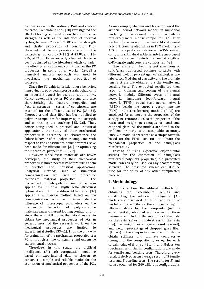
In the next step, the obtained results are used to construct the neural network models. Two separate networks are founded in every section, one for estimation of Ec with respect to Er, wt% of sand, and wt% of glass fiber, and another for estimation of σuc with respect to σur, wt% of sand, and wt% of glass fiber. The modulus of elasticity for both resin and composite (Er and Ec) are in GPa and the ultimate tensile stresses for both resin and composite (σur and σuc) are in MPa. The datasets are divided into two categories consisting of train and test datasets. For the below explained structures of the utilized neural networks, the components of the networks, including weight and bias terms, are acquired via an optimization process to fit the training dataset results in the training procedure. After the training procedure, the network should be tested over the test datasets. The testing observation datasets are not used in training and preserved for testing the generality of the neural network model. The same procedure of training and testing is performed for the ALM model as well. The generality of a method means that the method should give proper results for any other data other than the training data. In this study, 80% of the results are taken as the training datasets (192 observations) and the rest are left for testing of the networks (48 observations). A flow chart of the computational procedure is shown in Fig. 1.
Fig. 1. A flow chart for prediction of mechanical properties
of polymer concrete
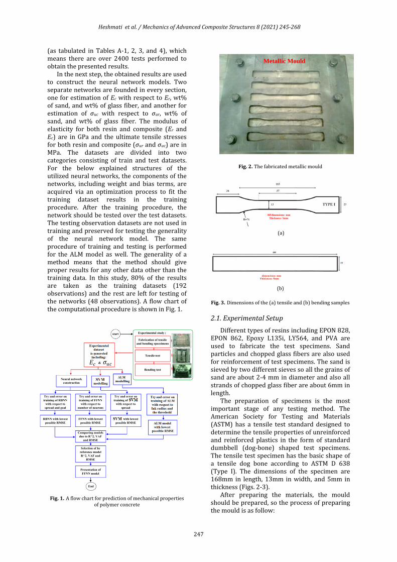
Metallic Mould
Fig. 2. The fabricated metallic mould
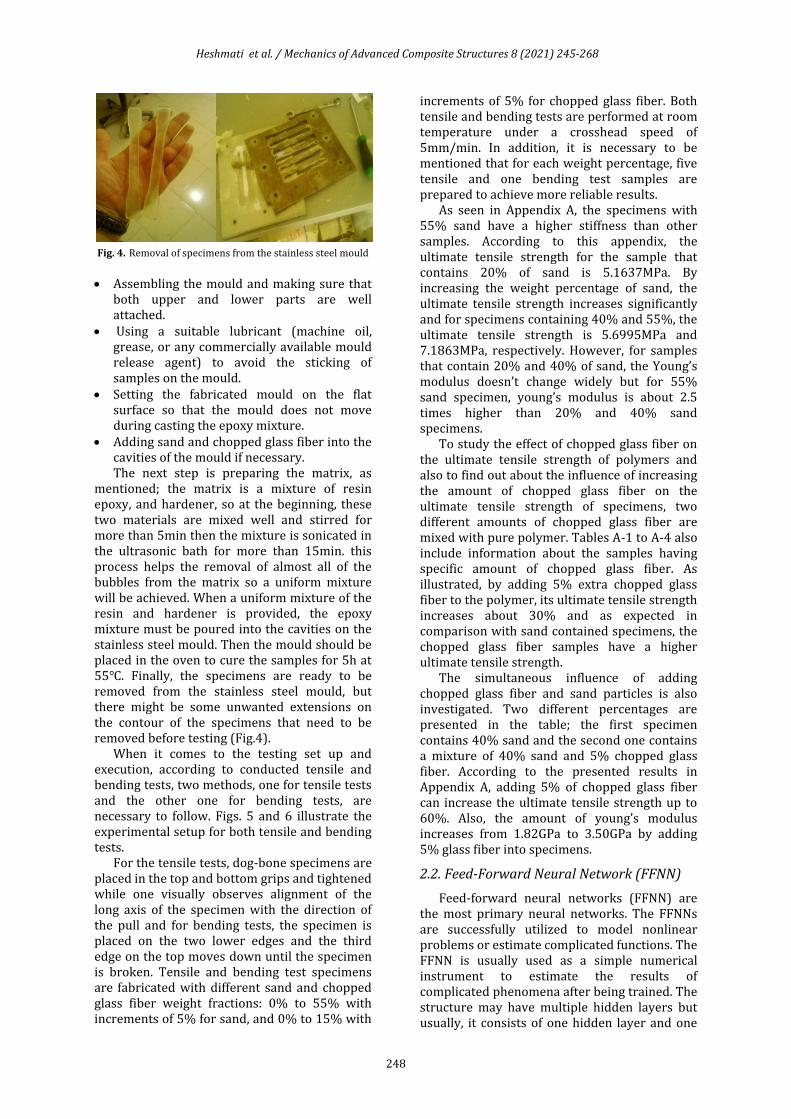
All dimensions: mm
Thickness: 5mm
(a)
(b)
Fig. 3. Dimensions of the (a) tensile and (b) bending samples
2.1. Experimental Setup
Different types of resins including EPON 828, EPON 862, Epoxy L135i, LY564, and PVA are used to fabricate the test specimens. Sand particles and chopped glass fibers are also used for reinforcement of test specimens. The sand is sieved by two different sieves so all the grains of sand are about 2-4 mm in diameter and also all strands of chopped glass fiber are about 6mm in length.
The preparation of specimens is the most important stage of any testing method. The American Society for Testing and Materials (ASTM) has a tensile test standard designed to determine the tensile properties of unreinforced and reinforced plastics in the form of standard dumbbell (dog-bone) shaped test specimens. The tensile test specimen has the basic shape of a tensile dog bone according to ASTM D 638 (Type I). The dimensions of the specimen are 168mm in length, 13mm in width, and 5mm in thickness (Figs. 2-3).
After preparing the materials, the mould should be prepared, so the process of preparing the mould is as follow:
Heshmati et al. / Mechanics of Advanced Composite Structures 8 (2021) 245-268
248
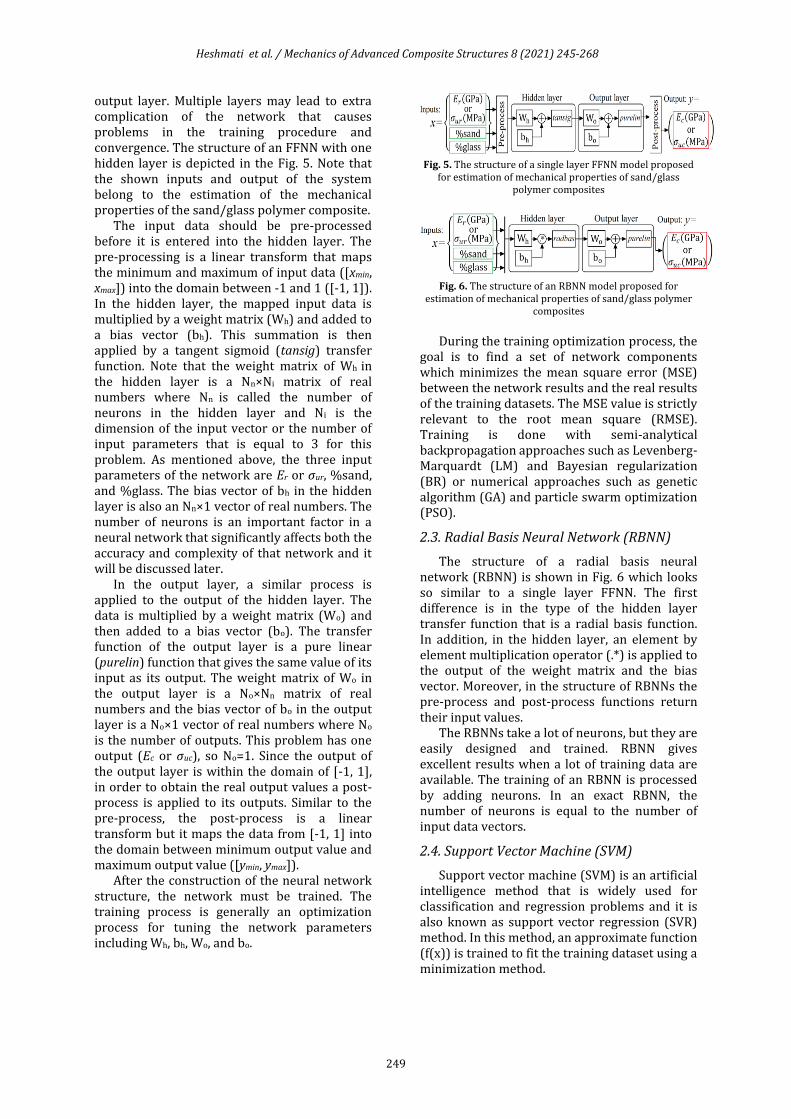
Fig. 4. Removal of specimens from the stainless steel mould
• Assembling the mould and making sure that both upper and lower parts are well attached.
• Using a suitable lubricant (machine oil, grease, or any commercially available mould release agent) to avoid the sticking of samples on the mould.
• Setting the fabricated mould on the flat surface so that the mould does not move during casting the epoxy mixture.
• Adding sand and chopped glass fiber into the cavities of the mould if necessary. The next step is preparing the matrix, as
mentioned; the matrix is a mixture of resin epoxy, and hardener, so at the beginning, these two materials are mixed well and stirred for more than 5min then the mixture is sonicated in the ultrasonic bath for more than 15min. this process helps the removal of almost all of the bubbles from the matrix so a uniform mixture will be achieved. When a uniform mixture of the resin and hardener is provided, the epoxy mixture must be poured into the cavities on the stainless steel mould. Then the mould should be placed in the oven to cure the samples for 5h at 55℃. Finally, the specimens are ready to be removed from the stainless steel mould, but there might be some unwanted extensions on the contour of the specimens that need to be removed before testing (Fig.4).
When it comes to the testing set up and execution, according to conducted tensile and bending tests, two methods, one for tensile tests and the other one for bending tests, are necessary to follow. Figs. 5 and 6 illustrate the experimental setup for both tensile and bending tests.
For the tensile tests, dog-bone specimens are placed in the top and bottom grips and tightened while one visually observes alignment of the long axis of the specimen with the direction of the pull and for bending tests, the specimen is placed on the two lower edges and the third edge on the top moves down until the specimen is broken. Tensile and bending test specimens are fabricated with different sand and chopped glass fiber weight fractions: 0% to 55% with increments of 5% for sand, and 0% to 15% with
increments of 5% for chopped glass fiber. Both tensile and bending tests are performed at room temperature under a crosshead speed of 5mm/min. In addition, it is necessary to be mentioned that for each weight percentage, five tensile and one bending test samples are prepared to achieve more reliable results.
As seen in Appendix A, the specimens with 55% sand have a higher stiffness than other samples. According to this appendix, the ultimate tensile strength for the sample that contains 20% of sand is 5.1637MPa. By increasing the weight percentage of sand, the ultimate tensile strength increases significantly and for specimens containing 40% and 55%, the ultimate tensile strength is 5.6995MPa and 7.1863MPa, respectively. However, for samples that contain 20% and 40% of sand, the Young’s modulus doesn’t change widely but for 55% sand specimen, young’s modulus is about 2.5 times higher than 20% and 40% sand specimens.
To study the effect of chopped glass fiber on the ultimate tensile strength of polymers and also to find out about the influence of increasing the amount of chopped glass fiber on the ultimate tensile strength of specimens, two different amounts of chopped glass fiber are mixed with pure polymer. Tables A-1 to A-4 also include information about the samples having specific amount of chopped glass fiber. As illustrated, by adding 5% extra chopped glass fiber to the polymer, its ultimate tensile strength increases about 30% and as expected in comparison with sand contained specimens, the chopped glass fiber samples have a higher ultimate tensile strength.
The simultaneous influence of adding chopped glass fiber and sand particles is also investigated. Two different percentages are presented in the table; the first specimen contains 40% sand and the second one contains a mixture of 40% sand and 5% chopped glass fiber. According to the presented results in Appendix A, adding 5% of chopped glass fiber can increase the ultimate tensile strength up to 60%. Also, the amount of young’s modulus increases from 1.82GPa to 3.50GPa by adding 5% glass fiber into specimens.
2.2. Feed-Forward Neural Network (FFNN)
Feed-forward neural networks (FFNN) are the most primary neural networks. The FFNNs are successfully utilized to model nonlinear problems or estimate complicated functions. The FFNN is usually used as a simple numerical instrument to estimate the results of complicated phenomena after being trained. The structure may have multiple hidden layers but usually, it consists of one hidden layer and one
Heshmati et al. / Mechanics of Advanced Composite Structures 8 (2021) 245-268
249
output layer. Multiple layers may lead to extra complication of the network that causes problems in the training procedure and convergence. The structure of an FFNN with one hidden layer is depicted in the Fig. 5. Note that the shown inputs and output of the system belong to the estimation of the mechanical properties of the sand/glass polymer composite.
The input data should be pre-processed before it is entered into the hidden layer. The pre-processing is a linear transform that maps the minimum and maximum of input data ([xmin, xmax]) into the domain between -1 and 1 ([-1, 1]). In the hidden layer, the mapped input data is multiplied by a weight matrix (Wh) and added to a bias vector (bh). This summation is then applied by a tangent sigmoid (tansig) transfer function. Note that the weight matrix of Wh in the hidden layer is a Nn×Ni matrix of real numbers where Nn is called the number of neurons in the hidden layer and Ni is the dimension of the input vector or the number of input parameters that is equal to 3 for this problem. As mentioned above, the three input parameters of the network are Er or σur, %sand, and %glass. The bias vector of bh in the hidden layer is also an Nn×1 vector of real numbers. The number of neurons is an important factor in a neural network that significantly affects both the accuracy and complexity of that network and it will be discussed later.
In the output layer, a similar process is applied to the output of the hidden layer. The data is multiplied by a weight matrix (Wo) and then added to a bias vector (bo). The transfer function of the output layer is a pure linear (purelin) function that gives the same value of its input as its output. The weight matrix of Wo in the output layer is a No×Nn matrix of real numbers and the bias vector of bo in the output layer is a No×1 vector of real numbers where No
is the number of outputs. This problem has one output (Ec or σuc), so No=1. Since the output of the output layer is within the domain of [-1, 1], in order to obtain the real output values a post-process is applied to its outputs. Similar to the pre-process, the post-process is a linear transform but it maps the data from [-1, 1] into the domain between minimum output value and maximum output value ([ymin, ymax]).
After the construction of the neural network structure, the network must be trained. The training process is generally an optimization process for tuning the network parameters including Wh, bh, Wo, and bo.
Fig. 5. The structure of a single layer FFNN model proposed
for estimation of mechanical properties of sand/glass polymer composites
Fig. 6. The structure of an RBNN model proposed for
estimation of mechanical properties of sand/glass polymer composites
During the training optimization process, the goal is to find a set of network components which minimizes the mean square error (MSE) between the network results and the real results of the training datasets. The MSE value is strictly relevant to the root mean square (RMSE). Training is done with semi-analytical backpropagation approaches such as Levenberg-Marquardt (LM) and Bayesian regularization (BR) or numerical approaches such as genetic algorithm (GA) and particle swarm optimization (PSO).
2.3. Radial Basis Neural Network (RBNN)
The structure of a radial basis neural network (RBNN) is shown in Fig. 6 which looks so similar to a single layer FFNN. The first difference is in the type of the hidden layer transfer function that is a radial basis function. In addition, in the hidden layer, an element by element multiplication operator (.*) is applied to the output of the weight matrix and the bias vector. Moreover, in the structure of RBNNs the pre-process and post-process functions return their input values.
The RBNNs take a lot of neurons, but they are easily designed and trained. RBNN gives excellent results when a lot of training data are available. The training of an RBNN is processed by adding neurons. In an exact RBNN, the number of neurons is equal to the number of input data vectors.
2.4. Support Vector Machine (SVM)
Support vector machine (SVM) is an artificial intelligence method that is widely used for classification and regression problems and it is also known as support vector regression (SVR) method. In this method, an approximate function (f(x)) is trained to fit the training dataset using a minimization method.

Heshmati et al. / Mechanics of Advanced Composite Structures 8 (2021) 245-268
250
Fig. 7. The structure of an SVM model proposed for
estimation of mechanical properties of sand/glass polymer composites
The structure of the constructed support vector machine in this study is illustrated in Fig. 7 which takes the resin properties (Er or σur) and weight percentages of sand and glass as inputs and gives the mechanical properties of the sand/glass polymer resin composites (Ec or σuc) as the output. In Fig. 7, the parameters αi and αi
∗ are the Lagrangian multipliers, N is the number of observations and K(xi, x) is the kernel function.
2.5. Active Learning Method (ALM (
ALM is a fuzzy regression algorithm, which works well in uncertain environments [44]. The basic idea of this algorithm is breaking a Multiple Input-Multiple Output (MIMO) system into several simpler Single Input-Single Output (SISO) subsystems as shown in Fig. 8.(a). Afterward, the algorithm combines these subsystems by a fuzzy inference engine in order to achieve the overall behavior of the system. Fig. 8.(b) shows a SISO subsystem of the ALM algorithm called Ink-Drop-Spread (IDS), where two valuable information (Narrow-Path and Spread)are extracted from it. Narrow-Path (NP) and Spread (SP) extracted from each SISO subsystem are then combined by a fuzzy inference unit. Equation (1) shows how these pieces of information are combined. Parameter 𝛹𝑖𝑗 is the NP of each SISO subsystem and𝛽𝑖𝑗is the
confidence degree of the NP and can be computed by Eq.(2). The ALM algorithm also considers the uncertainty for each data point by using a fuzzy membership function called an ink, as shown in fig. 8.(c). Fig. 8.(d) shows the ink drop spread of 7 data points in an IDS unit. It also shows NP and SP resulted from the IDS unit.
Fig. 8. (a) ALM algorithm breaks a multi-input-single-output function into simpler single-input-single output subsystems
and combines the results by a fuzzy inference engine. (b) Each single-input-single-output subsystem consists of a plan called an IDS plan and a feature extractor unit which extract
two useful pieces of information, Narrow Path (NP) and Spread (SP). (c) The Gaussian membership function which is
called an ink. This membership function is considered for each data point in every IDS plans. (d) The inks of 7 data
points are spread in an IDS plan which forms a pattern. The NP and SP are extracted from the IDS plan.
𝑦(𝑥) = 𝛽11𝛹11 + ⋯ + 𝛽𝑖𝑘𝛹𝑖𝑘 + ⋯ + 𝛽𝑛𝑙𝑛𝛹𝑛𝑙𝑛
(1)
where
𝛽𝑖𝑗 =
1
𝑆𝑖𝑗𝛤𝑖𝑗
1
𝑆11𝛤11 + ⋯ +
1
𝑆𝑖𝑗𝛤𝑖𝑗 + ⋯ +
1
𝑆𝑛𝑙𝑛
𝛤𝑛𝑙𝑛
(2)
where 1
𝑆𝑖𝑗is the Spread inverse and 𝛤𝑖𝑗 is the
membership degree of the data point to each SISO subsystem.
The Narrow path could be obtained by the weighted-average method, as in equation (3).
𝜓𝑖(𝑥) = {𝑏 ∈ 𝑌| ∑ 𝑑(𝑥, 𝑦)
𝑏
𝑦=𝑦𝑚𝑖𝑛
≈ ∑ 𝑑(𝑥, 𝑦)
𝑦𝑚𝑎𝑥
𝑦=𝑏
},
(3)
where d(xi, y) is the darkness value of coordinate (xi, y). The Spread can be computed by equation (4).
𝑦(𝑥) = 𝛽11𝛹11 + ⋯ + 𝛽𝑖𝑘𝛹𝑖𝑘 + ⋯ + 𝛽𝑛𝑙𝑛𝛹𝑛𝑙𝑛
(4)
where Th is the threshold of the IDS plane which is set by the user (usually Th=0 for modeling purpose).
Until now, numerous successful applications of ALM have been reported in function approximation[45, 46], classification [47-49], clustering [50, 51] and control [45, 52-54]. However, in [55] they show that ALM shows its best advantage when a high level of uncertainty existed in the system.
Heshmati et al. / Mechanics of Advanced Composite Structures 8 (2021) 245-268
251
3. Model Construction and Evaluation
In this section, the neural network models are constructed and evaluated. The models including FFNN, RBNN, SVM, and ALM are trained and tested separately for estimation of Ec and σuc. The models are compared with each other in respect to regression plots and statistical indices such as R2, RMSE, and VAF that are introduced below.
3.1. FFNN Results
The FFNN model is founded and trained twice, once for estimation of Ec in respect to Er, %sand, and %glass and once for estimation of σuc in respect to σur, %sand, and %glass. The models are trained and tested, using 192 datasets for training and 48 datasets for testing, as follows.
3.1.1. FFNN Model for Estimation of Ec
To estimate the modulus of elasticity of the sand/glass polymer composite (Ec), the FFNN model with 8 neurons in the hidden layer (Nn=8) is founded. The number of neurons is attained through a try and error procedure for finding the most exact network with the simplest structure. Hence, different numbers of neurons are applied to the network several times and the convergence of the networks is investigated noting the training and testing datasets. Finally, a single layer FFNN with 8 neurons in the hidden layer was revealed to be the most convergent network. This model also satisfies the simplicity factor with an 8×3 matrix of Wh, an 8×1 vector of bh, a 1×8 matrix of Wo, and a 1×1 vector of bo that generally means 26 components.
The Bayesian-regularization (BR) algorithm is used for training the network which is a fast and exact algorithm. The BR method is essentially a gradient-based method that chooses the first set of network components vector by random. Therefore, every time the BR method solves the problem, it gives different results for the network components. In order to achieve the best possible structure, the training process with the BR method is performed multiple times.
The statistical convergence indices of the finally achieved FFNN for training and testing datasets are shown in Table 1. The regression plots in Fig. 11 show the convergence between the experimental values of Ec and the FFNN results. Noting Fig. 11, the FFNN model gives proper results for both train and test datasets. Therefore, the constructed FFNN model seems to be an exact and general model for the problem. Further model evaluation is presented in the following sections.
3.1.2. FFNN Model for Estimation of σuc
To estimate the ultimate tensile stress of the sand/glass polymer composite (σuc), a similar FFNN with 11 neurons in the hidden layer is founded and trained. The statistical indices for comparison of the experimental results with the network results are given in Table 2. The same try and error procedure is applied for training the FFNN with the BR method. The indices show a proper accuracy for the network while the accuracy has a fall in comparison to the previous network.
3.2. RBNN Results
Similar to the previous section, the RBNN structure is constructed and trained once for estimation of the Ec with respect to Er, %sand, and %glass and once for estimation of σuc in respect to σur, %sand, and %glass. The training and testing results are primarily investigated with respect to the mentioned statistical indices.
3.2.1. RBNN Model for Estimation of Ec
For estimation of the modulus of elasticity of the composite, an RBNN with 56 neurons in the hidden layer is created. In order to reach the best accuracy, the spread value of the radial basis layer is taken equal to 10 and the goal mean squared error is taken equal to 0.01. These values for spread and goal are obtained through a try and error process.
The resulted indices for the RBNN results in comparison to the experimentally achieved composite modulus of elasticity are depicted in Table 1. The results show an excellent convergence and generality for the RBNN model.
3.2.2. RBNN Model for Estimation of σuc
A similar RBNN structure for estimation of the ultimate tensile stress of the composite is constructed with 111 neurons in the hidden layer. In order to reach the best accuracy, the spread value of the radial basis layer is taken equal to 8 and the goal mean square error is taken equal to 0.6. The values are obtained after a try and error process.
The statistical indices comparing the RBNN results with the experimentally achieved composite ultimate tensile stress are shown in Table 2. The results show an excellent convergence and a good generality for the RBNN model.
3.3. SVM Results
In this study, the Gaussian kernel function is utilized for the constructed SVM model. The parameter b is the threshold of the SVM system known as the bias term. This structure estimates the problem through an f(x) function with a

Heshmati et al. / Mechanics of Advanced Composite Structures 8 (2021) 245-268
252
deviation of ε that is a predefined parameter for accuracy and it is set to be equal to 0.001 in this study. The L1QP solver is used to solve the minimization problem that gives an SVM structure with a set of 192×3 support vectors. All the mentioned SVM settings are achieved through a try and error process to give the best possible results.
3.3.1. SVM Model for Estimation of Ec
The achieved indices for comparison of SVM results with the experimentally resulted values for composite modulus of elasticity are shown in Table 1. The results show proper accuracy for both testing and training procedures.
3.3.2. SVM Model for Estimation of σuc
The indices comparing the SVM results with the experimental values of the composite ultimate tensile stress are shown in Table 2. The results show a poor convergence for the model in training and testing states despite the previous SVM model. Therefore, the SVM model seems not to be proper for this problem.
3.4. ALM Results
In this section, the ALM structure is used for estimation of the Ec with respect to Er, %sand, and %glass, and for estimation of σuc with respect to σur, %sand, and %glass. A primary evaluation is possible noting the regression plots.
3.4.1. ALM Model for Estimation of Ec
The achieved statistical indices for comparison of ALM results with the experimentally resulted values for composite modulus of elasticity are shown in Table 1. The results show an acceptable convergence for the model in the training domain and testing results. The number of partitions in the ALM algorithm is 4,7 and 1 for Er, %sand, and %glass respectively. The Ink radius is also 0.085 and the threshold value is 0.01.
3.4.2. ALM Model for Estimation of σuc
The convergence indices comparing the ALM results with the experimental values of the composite ultimate tensile stress are shown in Table 2. The results show proper accuracy for both testing and training procedures. The number of partitions in the ALM algorithm is 5, 11, and 2 for Er, %sand, and %glass respectively. The Ink radius is also 0.005 and the threshold value is 0.01.
3.5. Model Evaluation
Evaluation of the obtained models for estimation of the mechanical properties of sand/glass polymer composites is performed in
this section. In this regard, the selected performance indices are R2, RMSE, and variance account for (VAF) which their equations can be written as follows:
𝑅2 = 1 −∑ (y − y′)2𝑁
𝑖=1
∑ (y′ − y)2𝑁𝑖=1
(5)
𝑉𝐴𝐹 = [1 −𝑉𝑎𝑟(y − y′)
𝑉𝑎𝑟(y′)] × 100
(6)
RMSE = √1
N∑ (y-y')2N
i=1 (7)
where y and y′ are the predicted and measured values, respectively, ỹ is the mean of the y′ values and N is the total number of data. The model will be excellent if R2 = 1, VAF =100 and RMSE = 0.
In the following subsections, the different constructed neural network models are evaluated with respect to the above-mentioned indices. With respect to the statistical indices, the most accurate models are chosen for the problem.
3.5.1. Model Evaluation for Estimation of Ec
The statistical performance indices including R2, RMSE, and VAF for the developed neural network models for estimation of Ec are presented in Table 1. It is observed that the resulted indices for each model are presented for both training and testing datasets.
Since the testing process is much important for generality and even convergence analysis, here it is recommended to consider the testing results as the decisive factor to ascertain the most accurate models. Comparing the resulted indices show that the most accurate model is the RBNN model for estimation of Ec. This model gives an excellent convergence and generality due to both train and test results. The results of the FFNN model are in the next grade with a slight difference. However, the FFNN model still gives excellent accuracy and generality. The poorest results belong to the RBNN model which has acceptable performance for training datasets but it doesn’t give proper results for testing datasets.
Table 1. R2, RMSE, and VAF results of the developed models for estimation of Ec
Method State R2 VAF RMSE
FFNN Training 0.9980 99.7944 0.1008
Testing 0.9976 99.7621 0.1073
RBNN Training 0.9981 99.8113 0.0966
Testing 0.9929 99.2118 0.1970
SVM Training 0.9707 96.5334 0.4219
Testing 0.9249 90.8253 0.6911
ALM Training 0.9330 89.6778 0.6251
Testing 0.9068 87.9767 0.6850
Heshmati et al. / Mechanics of Advanced Composite Structures 8 (2021) 245-268
253
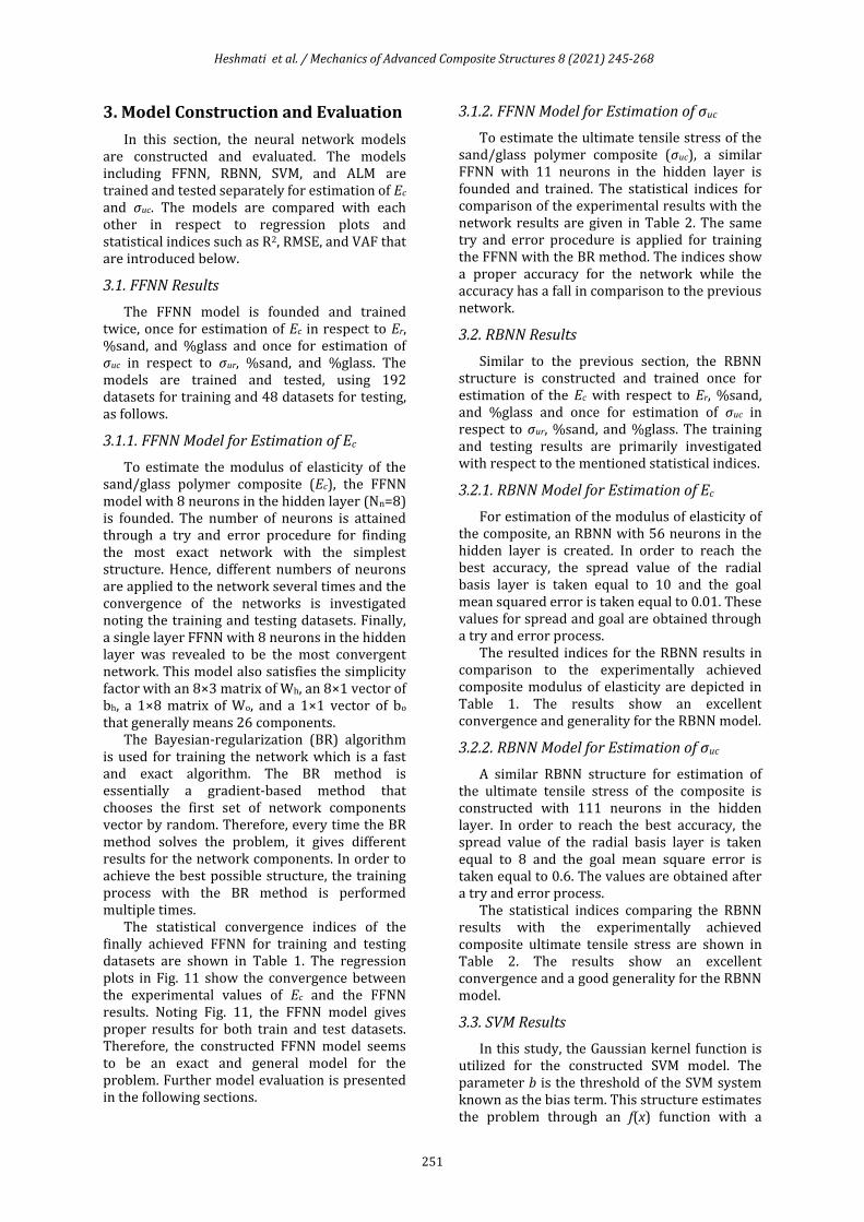
3.5.2. Model Evaluation for Estimation of σuc
The statistical performance indices including R2, RMSE, and VAF for the developed neural network models for estimation of σuc are presented in Table 2. The aforementioned statistical indices for each model are presented for both training and testing datasets.
Noting the performance indices for the testing process in Table 2, the FFNN model gives the best results for testing datasets. Whilst the RBNN model gives better results for the training process, the FFNN model seems to be the best choice for estimation of σuc and the RBNN model is in the next grade, because, as mentioned above, the testing results have higher importance. The SVM model can also be specified as the poorest model for estimation of σuc.
3.5.3. FFNN Model 5-Folds Cross Validation
The initial evaluation of models shows that the best accuracy and generality are achieved with an FFNN model. To ensure the generality of this model over all observations, a 5-fold cross validation is applied to the structure that is shown in Table 3 and 4 respectively for estimation of Ec and σuc based on mean R2 value.
In the 5-fold cross-validation process, the 240 observations are divided into 5 independent parts including 48 observations. Afterward, the model is trained and tested for 5 times (5 folds). In each fold, one of the separated parts is taken as the test data and the other 4 parts are taken as the training data. In this way, 100% of the dataset is used for both testing and training.
Table 2.R2, RMSE and VAF results of developed models for estimation of σuc
Method State R2 VAF RMSE
FFNN Training 0.9909 99.0883 1.2172
Testing 0.9904 99.0367 1.1310
RBNN Training 0.9963 99.6287 0.7740
Testing 0.9383 93.5807 2.9235
SVM Training 0.92 32 91.2052 3.0487
Testing 0.9129 90.2342 3.8952
ALM Training 0.9455 93.7121 3.0081
Testing 0.9357 91.5146 3.1182
Table 3. The mean R2 results for 5-fold cross-validation of FFNN for Ec estimation
State Mean R2
Fold 1 Fold 2 Fold 3 Fold 4 Fold 5 Average
Train 0.9980 0.9981 0.9952 0.9967 0.9918 0.9960
Test 0.9976 0.9957 0.9921 0.9907 0.9911 0.9934
Table 4. The mean R2 results for 5-fold cross-validation of FFNN model for σuc estimation
State Mean R2
Fold 1 Fold 2 Fold 3 Fold 4 Fold 5 Average
Train 0.9909 0.9881 0.9892 0.9896 0.9918 0.9899
Test 0.9904 0.9877 0.9889 0.9865 0.9911 0.9889
The 5-folds cross validation results are in a
closed range. Therefore, the results certify the generality of the FFNN model.
4. Model Presentation
In the previous sections, the models are constructed and investigated in terms of convergence and generality. The best models are chosen and it is time to represent proper models for obtaining the mechanical properties of sand/glass polymer composites. Since in addition to the accuracy the simplicity is an important factor in model presentation, for both estimation problems the FFNN model is presented that has a simple structure with excellent accuracy.
4.1. Model Presentation for Ec
An FFNN model proposed for estimation of the Ec is presented in this section. As mentioned above, in an FFNN model the input vector (x) at first should be mapped from [xmin, xmax] into the [-1, 1] domain through a linear function.
Due to the observations of the problem, the domain of [xmin, xmax] can be stated as 1.636≤Er
≤4 GPa, 0≤%sand≤55 percent, and 0≤%glass≤15 percent. Therefore, the mapped inputs (xp) can be obtained as follows.
−
=
−−−
−−−
−−−
=
==
1-%glass*1333.0
1-%sand*0364.0
3841.2*8460.0
1)0%glass()015(
2
1)0%sand()055(
2
1)636.1()636.14(
2
%glass
%sandmapmap
r
r
r
p
E
E
E
xx
(8)
Noting Fig. 5, the pre mapping output (yp) that is a value between -1 and 1 is obtained as follows.
( )( )ohho bb*Wtansig*W ++= pp xy (9)
The pre mapping output should then be mapped from [-1,1] into [ymin, ymax] domain where ymin=Ecmin= 1.5944 GPa and ymax=Ecmax =

Heshmati et al. / Mechanics of Advanced Composite Structures 8 (2021) 245-268
254
12.4596 GPa. Then the model output (Ec in GPa) will be obtained through a linear mapping as follows.
0270.74326.5
5944.1)1(2
5944.14596.12
(GPa)
+=
++−
=
=
p
p
c
y
y
Ey
(10)
Having the weight and bias matrices, this model can be applied to estimate the modulus of elasticity for sand/glass polymer composites (Ec) for any in-range datasets using any programming software. The weight and bias matrices are presented as follows.
=
. . .
. . -. -
. -. -. -
. . -. -
. . . -
. . .
. . . -
. . -. -
762106377407360
4645021221010820
134805663207060
4847099671121290
096002498213830
092517899403330
532800042003560
459300935013410
Wh
(11)
−
−
−
−
=
39975
56424
45610
17145
69550
63395
12090
08370
bh
.
.
.
.
.
.
.
.
(12)
T
−
−
−
−
−
=
9406.1
0322.2
5225.1
8148.1
4969.1
4125.1
4493.2
7097.2
Wo
(13)
67221bo .-= (14)
4.2. Model Presentation for σuc
An FFNN model proposed for estimation of the σuc is presented in this section. Similar to the previous model, at first, the input vector (x) should be mapped from [xmin, xmax] into the [-1, 1] domain through a linear function.
Due to the observations of the problem, the domain of [xmin, xmax] can be stated as 54.48≤σur≤93.540 MPa, 0≤%sand≤55 percent, and 0≤%glass≤15 percent. Therefore, the mapped inputs (xp) can be obtained as follows.
−
=
−−−
−−−
−−−
=
==
1-%glass*1333.0
1-%sand*0364.0
7891.3*0512.0
1)0%glass()015(
2
1)0%sand()055(
2
1)477.54()477.54541.93(
2
%glass
%sandmapmap
ur
uc
ur
p xx
(15)
Again, noting Fig. 5, the pre mapping output (yp) that is a value between -1 and 1 is obtained via Eq. 9.
The pre mapping output should then be mapped from [-1, 1] into [ymin, ymax] domain where ymin=σucmin = 7.7242 MPa and ymax=σucmax = 93.540 MPa. Then the model output (σuc in MPa) will be obtained through a linear mapping as follows.
6326.509084.42
7242.7)1(2
7242.75410.93
(MPa)
+=
++−
=
=
p
p
uc
y
y
y
(16)
Having the weight and bias matrices, this model can be applied to estimate the modulus of elasticity for sand/glass polymer composites (σuc) for any in-range datasets using any programming software. The weight and bias matrices are presented as follows.
=
877204163306660
092905180402390
042006023306740
243404071109630
550105997103890
305602938032640
360207500214660
376301999300840
028605189608490
288312824616550
710007976114180
Wh
. -. -.
. . .
. . -. -
. . -. -
. -. -.
. -. -. -
. -. . -
. -. -. -
. . -. -
. -. -.
. -. . -
(17)
=
85252
43281
66771
07242
26871
07600
59613
09301
67193
31938
67902
b h
.
. -
.
.
.
.
.
.
.
. -
.
(18)

Heshmati et al. / Mechanics of Advanced Composite Structures 8 (2021) 245-268
255
T
−
−
−
−
−
−
=
7538.0
0844.2
8197.2
9297.1
9318.1
5460.0
1773.2
8026.1
6380.1
5465.2
2044.1
Wo
(19)
95190bo .= (20)
5. Conclusions
In this study, the neural network soft computation modeling based on experimental datasets is used to construct a realistic model for the prediction of mechanical properties of sand/glass polymer composites. The tensile and bending tests are conducted to obtain the modulus of elasticity and the ultimate tensile stress of sand/glass reinforced polymer composite specimens. The extracted results are then used for training and testing of the neural network models. The model is supposed to give the mechanical properties of the sand/glass polymer composite including the modulus of
elasticity and ultimate tensile stress in respect to the modulus of elasticity and ultimate tensile stress of the resin and weight percentages of sand and glass in the composite. The ALM and SVM models and two different types of neural networks including FFNN and RBNN are employed for generating a realistic model. All of the models are trained to fit the problem datasets properly through a try and error procedure. The try and error process is performed to minimize the resulted RMSE value as much as possible to obtain the most acceptable configuration of each model. Then, for both training and testing data, the extracted results of ALM, FFNN, RBNN, and SVM models are compared together in terms of accuracy using the statistical indices including R2, RMSE, and VAF. Noting the obtained statistical indices, although all the models are excellent over the training process, the FFNN model is selected as the reference model because of its accuracy over the test data and simple structure. Since the FFNN model gives the best coincidence over the test data, it has the best generality among the obtained models. Finally, the models are presented as a simple formula based on the FFNN structure to obtain the mechanical properties of the sand/glass polymer composite with an excellent agreement with the experimental results.
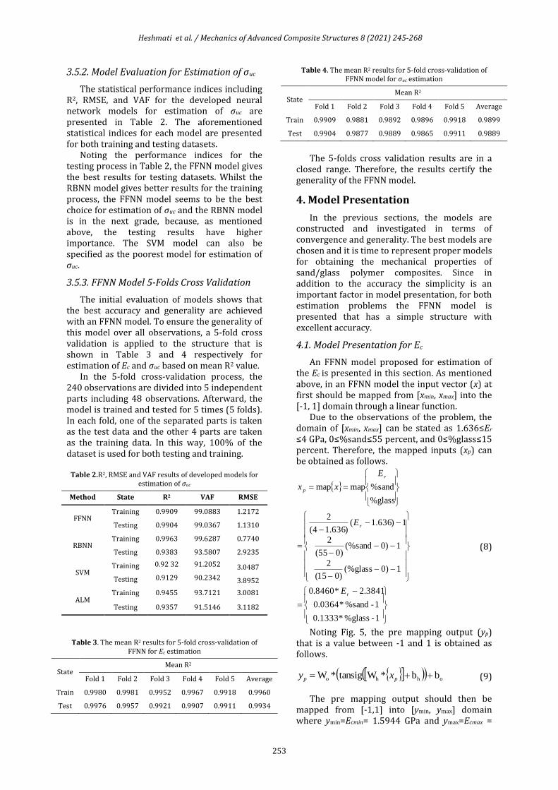
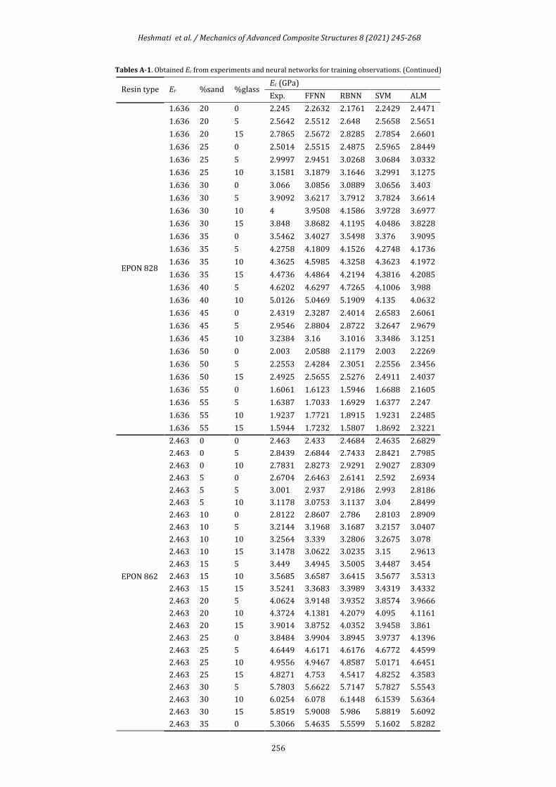
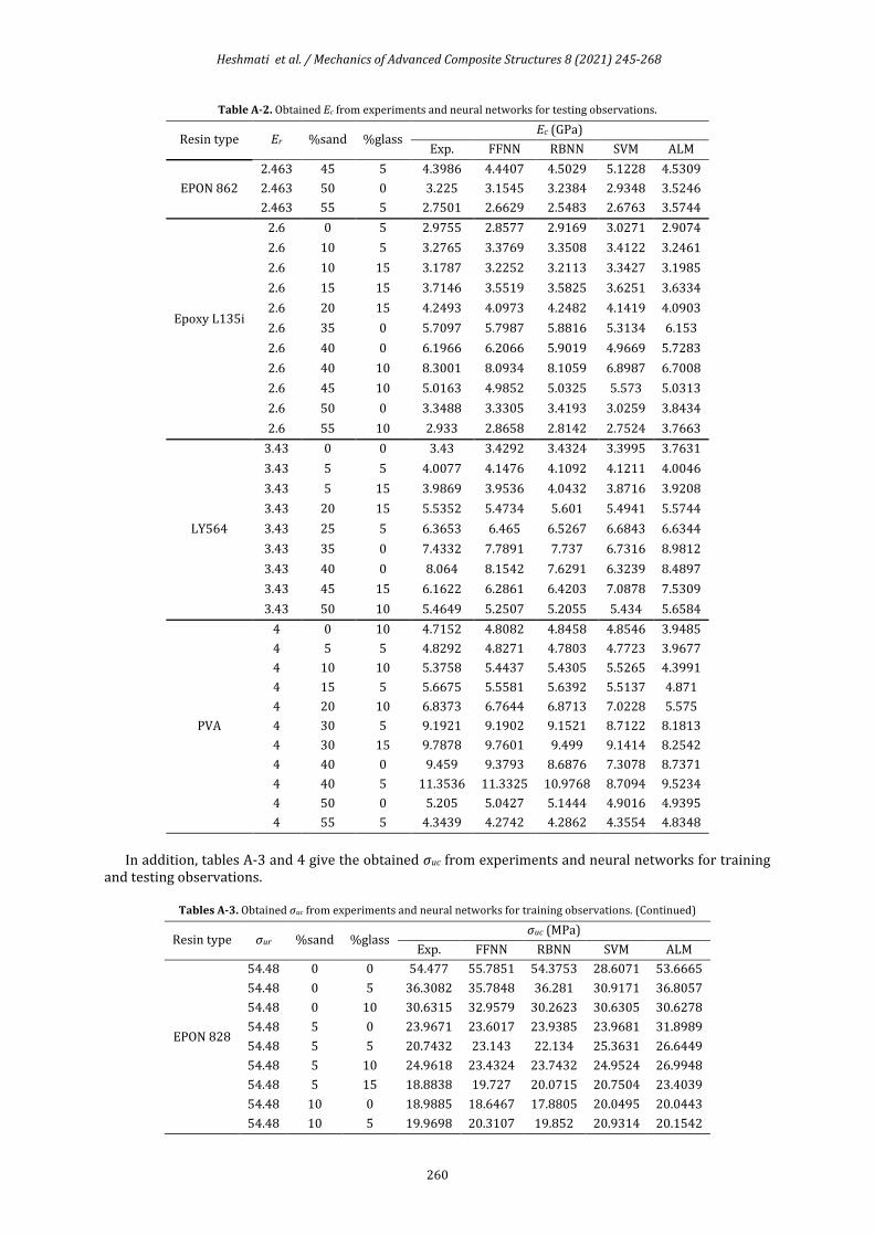
Appendix A
The experimentally obtained results for modulus of elasticity (Ec) and ultimate tensile stress of the sand glass resin composites (σuc) are tabulated in this section. The neural network results are also added to the tables to perform a comparison between the experimental results and the utilized neural networks. Tables A-1 and 2 give the obtained Ec from experiments and neural networks for training and testing observations.
Tables A-1. Obtained Ec from experiments and neural networks for training observations. (Continued)
Resin type Er %sand %glass Ec (GPa)
Exp. FFNN RBNN SVM ALM
EPON 828
1.636 0 0 1.636 1.4927 1.6348 1.6365 1.7654
1.636 0 5 1.705 1.6266 1.6996 1.706 1.8187
1.636 0 10 1.9529 1.8152 1.8873 1.9541 1.907
1.636 5 0 1.6457 1.7059 1.7794 1.6477 1.8151
1.636 5 5 1.8827 1.8651 1.8778 1.8823 1.875
1.636 5 10 2.1895 2.0329 2.0373 1.9893 1.9538
1.636 5 15 1.9656 1.9646 2.0446 1.9684 1.9512
1.636 10 0 1.8155 1.9014 1.9023 1.8277 2.0089
1.636 10 5 2.2046 2.0897 2.0609 2.137 2.1045
1.636 10 10 2.0862 2.2417 2.0656 2.146 2.1177
1.636 15 0 2.0789 2.0785 2.0488 2.0254 2.2255
1.636 15 5 2.3276 2.3052 2.356 2.3274 2.3392
1.636 15 10 2.3643 2.4532 2.4642 2.3658 2.2972
1.636 15 15 2.3162 2.3009 2.3186 2.3152 2.3881
Heshmati et al. / Mechanics of Advanced Composite Structures 8 (2021) 245-268
256
Tables A-1. Obtained Ec from experiments and neural networks for training observations. (Continued)
Resin type Er %sand %glass Ec (GPa)
Exp. FFNN RBNN SVM ALM
EPON 828
1.636 20 0 2.245 2.2632 2.1761 2.2429 2.4471
1.636 20 5 2.5642 2.5512 2.648 2.5658 2.5651
1.636 20 15 2.7865 2.5672 2.8285 2.7854 2.6601
1.636 25 0 2.5014 2.5515 2.4875 2.5965 2.8449
1.636 25 5 2.9997 2.9451 3.0268 3.0684 3.0332
1.636 25 10 3.1581 3.1879 3.1646 3.2991 3.1275
1.636 30 0 3.066 3.0856 3.0889 3.0656 3.403
1.636 30 5 3.9092 3.6217 3.7912 3.7824 3.6614
1.636 30 10 4 3.9508 4.1586 3.9728 3.6977
1.636 30 15 3.848 3.8682 4.1195 4.0486 3.8228
1.636 35 0 3.5462 3.4027 3.5498 3.376 3.9095
1.636 35 5 4.2758 4.1809 4.1526 4.2748 4.1736
1.636 35 10 4.3625 4.5985 4.3258 4.3623 4.1972
1.636 35 15 4.4736 4.4864 4.2194 4.3816 4.2085
1.636 40 5 4.6202 4.6297 4.7265 4.1006 3.988
1.636 40 10 5.0126 5.0469 5.1909 4.135 4.0632
1.636 45 0 2.4319 2.3287 2.4014 2.6583 2.6061
1.636 45 5 2.9546 2.8804 2.8722 3.2647 2.9679
1.636 45 10 3.2384 3.16 3.1016 3.3486 3.1251
1.636 50 0 2.003 2.0588 2.1179 2.003 2.2269
1.636 50 5 2.2553 2.4284 2.3051 2.2556 2.3456
1.636 50 15 2.4925 2.5655 2.5276 2.4911 2.4037
1.636 55 0 1.6061 1.6123 1.5946 1.6688 2.1605
1.636 55 5 1.6387 1.7033 1.6929 1.6377 2.247
1.636 55 10 1.9237 1.7721 1.8915 1.9231 2.2485
1.636 55 15 1.5944 1.7232 1.5807 1.8692 2.3221
EPON 862
2.463 0 0 2.463 2.433 2.4684 2.4635 2.6829
2.463 0 5 2.8439 2.6844 2.7433 2.8421 2.7985
2.463 0 10 2.7831 2.8273 2.9291 2.9027 2.8309
2.463 5 0 2.6704 2.6463 2.6141 2.592 2.6934
2.463 5 5 3.001 2.937 2.9186 2.993 2.8186
2.463 5 10 3.1178 3.0753 3.1137 3.04 2.8499
2.463 10 0 2.8122 2.8607 2.786 2.8103 2.8909
2.463 10 5 3.2144 3.1968 3.1687 3.2157 3.0407
2.463 10 10 3.2564 3.339 3.2806 3.2675 3.078
2.463 10 15 3.1478 3.0622 3.0235 3.15 2.9613
2.463 15 5 3.449 3.4945 3.5005 3.4487 3.454
2.463 15 10 3.5685 3.6587 3.6415 3.5677 3.5313
2.463 15 15 3.5241 3.3683 3.3989 3.4319 3.4332
2.463 20 5 4.0624 3.9148 3.9352 3.8574 3.9666
2.463 20 10 4.3724 4.1381 4.2079 4.095 4.1161
2.463 20 15 3.9014 3.8752 4.0352 3.9458 3.861
2.463 25 0 3.8484 3.9904 3.8945 3.9737 4.1396
2.463 25 5 4.6449 4.6171 4.6176 4.6772 4.4599
2.463 25 10 4.9556 4.9467 4.8587 5.0171 4.6451
2.463 25 15 4.8271 4.753 4.5417 4.8252 4.3583
2.463 30 5 5.7803 5.6622 5.7147 5.7827 5.5543
2.463 30 10 6.0254 6.078 6.1448 6.1539 5.6364
2.463 30 15 5.8519 5.9008 5.986 5.8819 5.6092
2.463 35 0 5.3066 5.4635 5.5599 5.1602 5.8282

Heshmati et al. / Mechanics of Advanced Composite Structures 8 (2021) 245-268
257
Tables A-1. Obtained Ec from experiments and neural networks for training observations. (Continued)
Resin type Er %sand %glass Ec (GPa)
Exp. FFNN RBNN SVM ALM
EPON 862
2.463 35 10 6.8829 6.8376 6.7699 6.8825 6.4567
2.463 35 15 6.5651 6.5656 6.4596 6.5632 6.1684
2.463 40 0 5.7196 5.8664 5.5984 4.846 5.3591
2.463 40 5 7.1168 7.1167 7.049 6.3204 6.2489
2.463 40 10 7.6231 7.6578 7.6916 6.6002 6.3492
2.463 40 15 7.1352 7.1898 7.3245 6.3382 5.971
2.463 45 0 3.9122 3.7537 3.8314 3.9129 3.87
2.463 45 10 4.8061 4.7216 4.7564 5.3242 4.7573
2.463 45 15 4.5947 4.5545 4.5038 5.18 3.9366
2.463 50 5 3.652 3.6789 3.5364 3.6504 3.7142
2.463 50 10 3.7404 3.738 3.7761 3.7385 3.834
2.463 50 15 3.6405 3.6337 3.6358 3.6383 3.6357
2.463 55 0 2.5412 2.4521 2.4224 2.432 3.5049
2.463 55 10 2.6259 2.71 2.6741 2.6262 3.6745
2.463 55 15 2.4299 2.4547 2.3685 2.4295 3.5162
Epoxy L135i
2.6 0 0 2.6 2.5812 2.6064 2.5991 2.7867
2.6 0 10 3.1194 2.9997 3.1026 3.121 2.9346
2.6 0 15 2.9468 2.7743 2.9128 2.9467 2.9332
2.6 5 0 2.7303 2.7942 2.7514 2.7415 2.8477
2.6 5 5 3.0418 3.112 3.0899 3.1824 2.9744
2.6 5 10 3.166 3.2522 3.2901 3.2709 3.0045
2.6 5 15 3.1216 2.9852 3.1413 3.1193 3.0188
2.6 10 0 2.8117 3.0112 2.9313 2.9677 3.0873
2.6 10 10 3.5155 3.5242 3.4798 3.5038 3.2769
2.6 15 0 3.2326 3.2581 3.2099 3.1963 3.4633
2.6 15 5 3.6653 3.6872 3.6923 3.6652 3.6542
2.6 15 10 3.8056 3.8607 3.8405 3.8082 3.7089
2.6 20 0 3.5402 3.6096 3.5425 3.5413 3.9113
2.6 20 5 4.1882 4.1348 4.1551 4.1042 4.1351
2.6 20 10 4.4512 4.3733 4.4344 4.3451 4.2332
2.6 25 0 4.0574 4.2168 4.1284 4.1603 4.4472
2.6 25 5 4.8616 4.8865 4.8865 4.951 4.7739
2.6 25 10 5.1115 5.2371 5.15 5.2878 4.8772
2.6 25 15 4.8537 5.0351 4.8293 5.0442 4.668
2.6 30 0 5.1853 5.1736 5.0724 4.9129 5.3885
2.6 30 5 5.9575 5.9919 6.0316 6.0648 5.8528
2.6 30 10 6.5311 6.4291 6.4769 6.4522 5.9409
2.6 30 15 6.4493 6.2417 6.3004 6.1406 5.9604
2.6 35 5 6.8684 6.7632 6.8863 6.8076 6.7436
2.6 35 10 7.1974 7.2114 7.1748 7.1968 6.8096
2.6 35 15 6.8498 6.9184 6.836 6.8509 6.644
2.6 40 5 7.3229 7.5166 7.4234 6.5443 6.6028
2.6 40 15 7.5562 7.6067 7.7255 6.6157 6.2004
2.6 45 0 4.0099 3.9852 4.0569 4.0114 4.2799
2.6 45 5 4.7793 4.6979 4.7659 5.298 4.9381
2.6 45 15 4.8507 4.7917 4.7711 5.4058 4.2691
2.6 50 5 3.7119 3.8832 3.74 3.7827 3.8905

Heshmati et al. / Mechanics of Advanced Composite Structures 8 (2021) 245-268
258
Tables A-1. Obtained Ec from experiments and neural networks for training observations. (Continued)
Resin type Er %sand %glass Ec (GPa)
Exp. FFNN RBNN SVM ALM
LY564
2.6 50 10 3.8912 3.9507 3.9765 3.9225 3.946
2.6 50 15 3.822 3.8189 3.8267 3.7955 3.8779
2.6 55 0 2.5189 2.5835 2.5612 2.5216 3.7452
2.6 55 5 2.7755 2.8163 2.6968 2.7768 3.723
2.6 55 15 2.4778 2.5839 2.5091 2.5291 3.738
3.43 0 5 3.9318 3.8859 3.9613 3.9317 3.9038
3.43 0 10 4.1389 4.0647 4.1465 4.1375 3.981
3.43 0 15 3.6576 3.706 3.7671 3.6572 3.808
3.43 5 0 3.539 3.6385 3.5684 3.6065 3.8566
3.43 5 10 4.1923 4.341 4.3342 4.346 4.0849
3.43 10 0 3.8767 3.8689 3.7944 3.8752 4.132
3.43 10 5 4.4269 4.4393 4.4322 4.3774 4.2996
3.43 10 10 4.6294 4.6592 4.6593 4.6286 4.3861
3.43 10 15 4.1826 4.2566 4.3198 4.1836 4.2196
3.43 15 0 4.2495 4.1679 4.204 4.2088 4.693
3.43 15 5 4.7279 4.82 4.854 4.7755 4.9182
3.43 15 10 5.0503 5.0916 5.0561 5.0529 5.0258
3.43 15 15 4.6696 4.703 4.7096 4.66 4.7973
3.43 20 0 4.7226 4.6503 4.7316 4.7401 5.2515
3.43 20 5 5.5105 5.4253 5.5111 5.513 5.5699
3.43 20 10 5.8889 5.7961 5.8586 5.8288 5.6718
3.43 25 0 5.4549 5.5154 5.5325 5.539 6.0618
3.43 25 10 6.8253 6.9831 6.955 7.0986 6.5466
3.43 25 15 6.6779 6.7645 6.6235 6.7906 6.5953
3.43 30 0 6.791 6.8255 6.7031 6.3642 7.751
3.43 30 5 7.9667 7.9285 7.9152 7.967 8.3049
3.43 30 10 8.4853 8.5357 8.4788 8.567 8.316
3.43 30 15 8.2336 8.3231 8.2089 8.2346 8.2492
3.43 35 5 9.1141 8.9359 9.1224 8.6622 9.0615
3.43 35 10 9.462 9.4791 9.5938 9.4653 9.1691
3.43 35 15 9.0873 9.0961 9.1158 9.0868 9.0391
3.43 40 5 9.7099 9.8435 9.5985 8.2205 9.5546
3.43 40 10 10.8167 10.7154 10.5818 9.1011 9.7884
3.43 40 15 10.2464 10.2184 10.1707 8.6959 9.6736
3.43 45 0 5.2811 5.3593 5.3371 5.3021 6.0204
3.43 45 5 6.1173 6.2425 6.2955 6.7522 7.0631
3.43 45 10 6.599 6.6053 6.6945 7.5012 7.6987
3.43 50 0 4.5152 4.3638 4.4731 4.1721 5.0545
3.43 50 5 4.9607 5.0995 4.9557 4.962 5.3887
3.43 50 15 4.9407 4.9868 5.0129 5.003 5.6358
3.43 55 0 3.3862 3.3337 3.4022 3.3867 4.7099
3.43 55 5 3.5763 3.706 3.6271 3.5948 4.8561
3.43 55 10 3.7944 3.8051 3.717 3.7943 4.8097
3.43 55 15 3.3383 3.4101 3.4118 3.3386 4.8492
PVA
4 0 0 4 3.9592 3.9811 4.0003 3.8007
4 0 5 4.6013 4.5632 4.6602 4.6004 3.8968
4 0 15 4.4557 4.3911 4.3377 4.4555 3.8314
4 5 0 4.1982 4.1646 4.106 4.1561 3.8687
4 5 10 5.1597 5.0978 5.0165 5.1591 4.0231
Heshmati et al. / Mechanics of Advanced Composite Structures 8 (2021) 245-268
259
Tables A-1. Obtained Ec from experiments and neural networks for training observations.
Resin type Er %sand %glass Ec (GPa)
Exp. FFNN RBNN SVM ALM
PVA
4 5 15 4.7092 4.6619 4.6259 4.7071 3.9494
4 10 0 4.4106 4.4024 4.3615 4.412 4.2307
4 10 5 5.0298 5.1338 5.1424 5.0297 4.3426
4 10 15 4.9868 5.0051 5.0408 5.0282 4.2441
4 15 0 4.8679 4.7342 4.868 4.8653 4.7266
4 15 10 6.0828 5.9364 5.8875 6.0821 4.9397
4 15 15 5.5673 5.529 5.4859 5.5489 4.8237
4 20 0 5.6188 5.3012 5.5359 5.6172 5.2944
4 20 5 6.4275 6.2644 6.4513 6.3716 5.4925
4 20 15 6.4571 6.446 6.5763 6.458 5.5386
4 25 0 6.3753 6.3349 6.4694 6.6046 6.2599
4 25 5 7.5661 7.4913 7.6465 7.5652 6.6674
4 25 10 8.1871 8.1613 8.2138 8.3889 6.5947
4 25 15 7.7807 7.968 7.8854 7.78 6.5056
4 30 0 7.8374 7.8783 7.7553 7.489 7.7987
4 30 10 10.0792 9.9509 9.8197 9.7948 8.1755
4 35 0 8.8822 9.1164 8.9 7.8053 9.1038
4 35 5 10.5631 10.3888 10.5569 9.2198 9.1202
4 35 10 10.8418 11.0276 11.1924 10.5051 9.1826
4 35 15 10.6245 10.6217 10.6513 9.8523 9.056
4 40 10 12.4596 12.4698 12.219 9.9536 9.6976
4 40 15 11.8771 12.0689 11.8353 9.3784 9.5952
4 45 0 6.1825 6.2744 6.1182 6.1809 6.3094
4 45 5 7.1191 7.2853 7.266 7.3399 7.2566
4 45 10 7.7798 7.7336 7.8053 8.2421 7.7183
4 45 15 7.4583 7.3657 7.5614 7.799 7.2397
4 50 5 5.8808 5.9096 5.76 5.6932 5.1144
4 50 10 6.0961 6.1474 6.0502 6.0943 5.2038
4 50 15 5.936 5.8294 5.8421 5.7838 5.4418
4 55 0 3.9123 3.8047 3.9711 3.9124 4.7411
4 55 10 4.321 4.4381 4.38 4.3235 4.8039
4 55 15 4.1128 4.0168 4.072 4.1138 4.8303
Table A-2. Obtained Ec from experiments and neural networks for testing observations. (Continued)
Resin type Er %sand %glass Ec (GPa)
Exp. FFNN RBNN SVM ALM
EPON 828
1.636 0 15 1.7508 1.8004 1.9141 2.1126 1.8776
1.636 10 15 2.1247 2.1247 1.8742 2.0401 2.1044
1.636 20 10 2.7668 2.7231 2.9085 2.7207 2.5751
1.636 25 15 3.1105 3.0738 2.8813 3.4164 3.0806
1.636 40 0 3.8226 3.704 3.6787 3.2345 3.5
1.636 40 15 4.7555 4.7846 4.9543 4.1572 4.0859
1.636 45 15 3.0413 3.1808 2.9428 3.406 2.6812
1.636 50 10 2.6192 2.4729 2.5973 2.4496 2.4043
EPON 862
2.463 0 15 2.5745 2.6286 2.7705 2.8015 2.7665
2.463 5 15 2.9489 2.8331 2.9878 2.9418 2.7988
2.463 15 0 3.037 3.0984 3.0444 3.0301 3.267
2.463 20 0 3.4213 3.4272 3.3463 3.363 3.7444
2.463 30 0 4.9297 4.8876 4.7948 4.7337 5.0843
2.463 35 5 6.5495 6.3992 6.5045 6.5435 6.4195
Heshmati et al. / Mechanics of Advanced Composite Structures 8 (2021) 245-268
260
Table A-2. Obtained Ec from experiments and neural networks for testing observations.
Resin type Er %sand %glass Ec (GPa)
Exp. FFNN RBNN SVM ALM
EPON 862
2.463 45 5 4.3986 4.4407 4.5029 5.1228 4.5309
2.463 50 0 3.225 3.1545 3.2384 2.9348 3.5246
2.463 55 5 2.7501 2.6629 2.5483 2.6763 3.5744
Epoxy L135i
2.6 0 5 2.9755 2.8577 2.9169 3.0271 2.9074
2.6 10 5 3.2765 3.3769 3.3508 3.4122 3.2461
2.6 10 15 3.1787 3.2252 3.2113 3.3427 3.1985
2.6 15 15 3.7146 3.5519 3.5825 3.6251 3.6334
2.6 20 15 4.2493 4.0973 4.2482 4.1419 4.0903
2.6 35 0 5.7097 5.7987 5.8816 5.3134 6.153
2.6 40 0 6.1966 6.2066 5.9019 4.9669 5.7283
2.6 40 10 8.3001 8.0934 8.1059 6.8987 6.7008
2.6 45 10 5.0163 4.9852 5.0325 5.573 5.0313
2.6 50 0 3.3488 3.3305 3.4193 3.0259 3.8434
2.6 55 10 2.933 2.8658 2.8142 2.7524 3.7663
LY564
3.43 0 0 3.43 3.4292 3.4324 3.3995 3.7631
3.43 5 5 4.0077 4.1476 4.1092 4.1211 4.0046
3.43 5 15 3.9869 3.9536 4.0432 3.8716 3.9208
3.43 20 15 5.5352 5.4734 5.601 5.4941 5.5744
3.43 25 5 6.3653 6.465 6.5267 6.6843 6.6344
3.43 35 0 7.4332 7.7891 7.737 6.7316 8.9812
3.43 40 0 8.064 8.1542 7.6291 6.3239 8.4897
3.43 45 15 6.1622 6.2861 6.4203 7.0878 7.5309
3.43 50 10 5.4649 5.2507 5.2055 5.434 5.6584
PVA
4 0 10 4.7152 4.8082 4.8458 4.8546 3.9485
4 5 5 4.8292 4.8271 4.7803 4.7723 3.9677
4 10 10 5.3758 5.4437 5.4305 5.5265 4.3991
4 15 5 5.6675 5.5581 5.6392 5.5137 4.871
4 20 10 6.8373 6.7644 6.8713 7.0228 5.575
4 30 5 9.1921 9.1902 9.1521 8.7122 8.1813
4 30 15 9.7878 9.7601 9.499 9.1414 8.2542
4 40 0 9.459 9.3793 8.6876 7.3078 8.7371
4 40 5 11.3536 11.3325 10.9768 8.7094 9.5234
4 50 0 5.205 5.0427 5.1444 4.9016 4.9395
4 55 5 4.3439 4.2742 4.2862 4.3554 4.8348
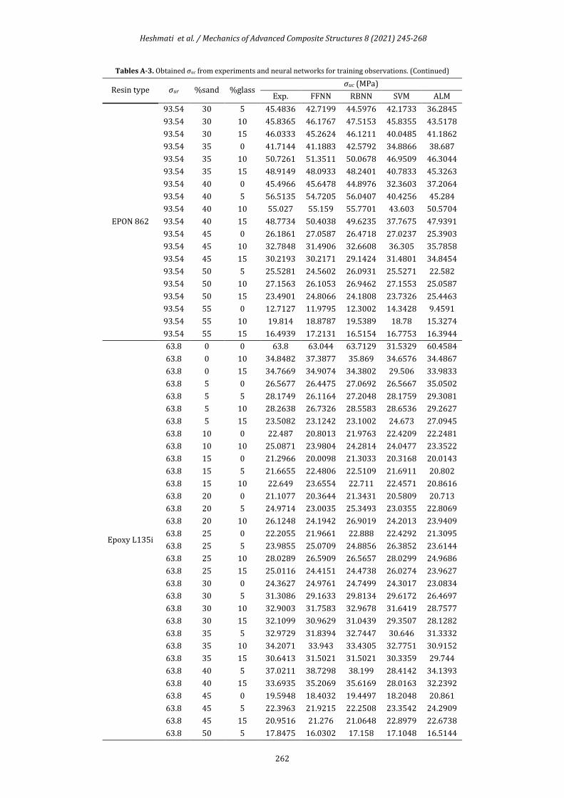
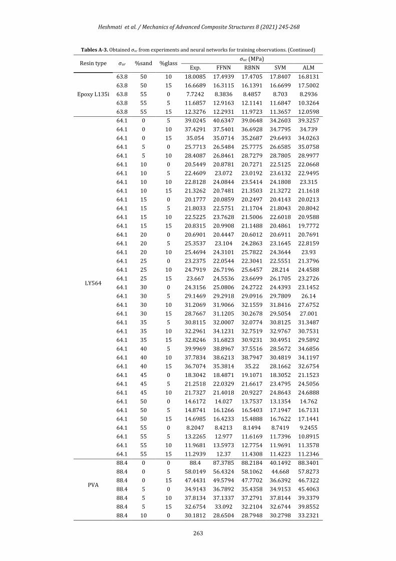
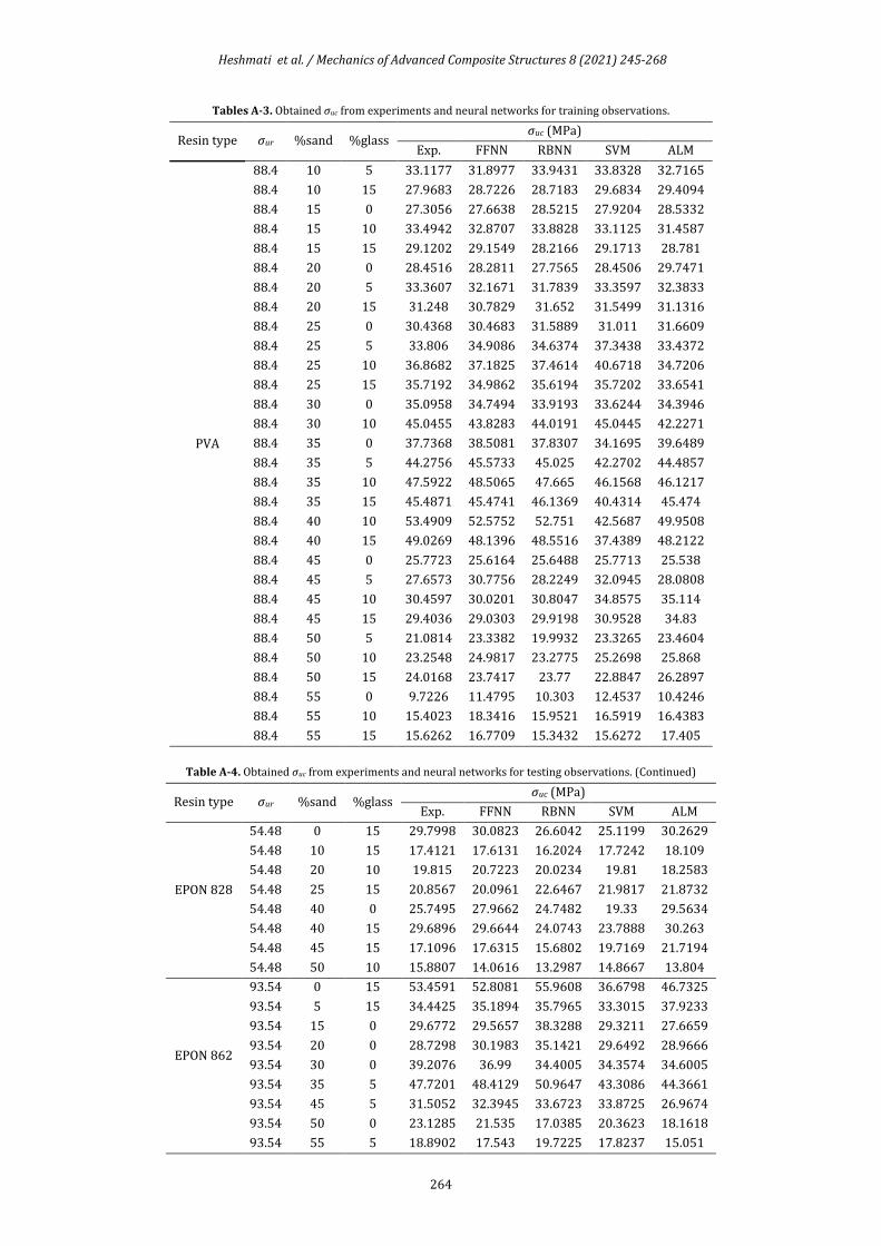
In addition, tables A-3 and 4 give the obtained σuc from experiments and neural networks for training
and testing observations.
Tables A-3. Obtained σuc from experiments and neural networks for training observations. (Continued)
Resin type σur %sand %glass σuc (MPa)
Exp. FFNN RBNN SVM ALM
EPON 828
54.48 0 0 54.477 55.7851 54.3753 28.6071 53.6665
54.48 0 5 36.3082 35.7848 36.281 30.9171 36.8057
54.48 0 10 30.6315 32.9579 30.2623 30.6305 30.6278
54.48 5 0 23.9671 23.6017 23.9385 23.9681 31.8989
54.48 5 5 20.7432 23.143 22.134 25.3631 26.6449
54.48 5 10 24.9618 23.4324 23.7432 24.9524 26.9948
54.48 5 15 18.8838 19.727 20.0715 20.7504 23.4039
54.48 10 0 18.9885 18.6467 17.8805 20.0495 20.0443
54.48 10 5 19.9698 20.3107 19.852 20.9314 20.1542

Heshmati et al. / Mechanics of Advanced Composite Structures 8 (2021) 245-268
261
Tables A-3. Obtained σuc from experiments and neural networks for training observations. (Continued)
Resin type σur %sand %glass σuc (MPa)
Exp. FFNN RBNN SVM ALM
EPON 828
54.48 10 10 20.5124 20.9277 20.2429 20.5134 20.8776
54.48 15 0 17.4221 17.868 18.9854 17.9012 18.3457
54.48 15 5 20.1246 19.7538 19.9211 18.9475 19.2034
54.48 15 10 17.567 20.4695 18.9727 18.7055 17.8761
54.48 15 15 15.9865 17.5942 15.6247 17.0617 15.9565
54.48 20 0 18.9492 18.0887 17.478 17.8208 18.6015
54.48 20 5 20.6194 20.0834 19.6531 19.6956 19.1031
54.48 20 15 18.828 17.7682 18.1349 18.827 18.128
54.48 25 0 17.1081 19.4391 18.8662 19.1736 19.2334
54.48 25 5 20.7538 21.8283 21.2736 22.2233 20.6393
54.48 25 10 21.5984 22.7008 21.8608 22.7783 21.4166
54.48 30 0 20.4189 21.9521 19.3074 20.6669 21.3748
54.48 30 5 24.758 25.3528 24.1084 24.759 23.7226
54.48 30 10 25.6786 27.2426 25.6839 25.6796 25.2638
54.48 30 15 27.6466 26.0401 27.6297 24.7952 26.3786
54.48 35 0 21.7471 22.4355 22.2766 20.9635 24.0444
54.48 35 5 29.2842 26.9983 29.5374 25.5543 28.3819
54.48 35 10 28.2461 28.4251 28.4495 26.6213 27.7278
54.48 35 15 25.6426 25.8751 26.1514 25.6436 26.3636
54.48 40 5 33.3239 33.6133 34.0794 23.7196 31.7746
54.48 40 10 33.0457 32.7273 31.3768 24.6625 31.5073
54.48 45 0 16.1209 15.9173 14.9302 15.9867 21.8652
54.48 45 5 19.5845 18.5203 19.6499 19.6182 24.7651
54.48 45 10 17.2612 17.5912 18.4914 20.2351 23.0804
54.48 50 0 10.6348 11.6598 10.8134 11.986 12.8481
54.48 50 5 12.8819 13.05 13.1761 14.6316 14.4276
54.48 50 15 14.863 12.643 14.0208 14.864 14.9535
54.48 55 0 8.6975 7.3014 9.1322 8.6985 9.4579
54.48 55 5 10.4607 11.0092 9.7274 10.4597 10.0063
54.48 55 10 8.8147 10.9916 8.9898 10.3994 9.0472
54.48 55 15 10.906 9.6831 11.3177 10.907 10.9876
EPON 862
93.54 0 0 93.541 93.4378 93.3295 41.0201 88.3401
93.54 0 5 58.8938 60.3845 59.2767 45.4663 57.9415
93.54 0 10 53.7847 54.8589 53.3707 43.0103 47.3515
93.54 5 0 38.8327 39.4758 39.2174 36.147 48.5309
93.54 5 5 40.1159 38.7513 39.3257 40.053 43.8171
93.54 5 10 39.343 39.4555 40.3507 38.5643 36.7395
93.54 10 0 31.7029 30.649 31.7127 31.7039 32.6646
93.54 10 5 32.7764 33.9836 32.9089 35.3533 31.9062
93.54 10 10 35.0161 35.1153 34.5275 35.0964 32.3582
93.54 10 15 30.8656 30.2336 30.6482 30.7828 28.9016
93.54 15 5 31.651 33.3235 31.467 33.338 30.0068
93.54 15 10 32.0249 34.7433 31.829 34.3984 32.0587
93.54 15 15 30.2123 30.6104 30.5439 30.4933 29.0847
93.54 20 5 35.5225 34.184 35.9735 34.7216 32.5291
93.54 20 10 36.9912 35.8382 37.4358 36.9902 31.2906
93.54 20 15 33.664 32.4064 33.7427 32.8 31.132
93.54 25 0 30.504 32.4715 30.1854 31.9404 30.9079
93.54 25 5 35.3162 37.0186 35.8027 38.4605 33.6806
93.54 25 10 38.9894 39.2488 37.7578 41.6442 36.9359
93.54 25 15 36.1733 36.869 35.9251 36.6757 34.2263
Heshmati et al. / Mechanics of Advanced Composite Structures 8 (2021) 245-268
262
Tables A-3. Obtained σuc from experiments and neural networks for training observations. (Continued)
Resin type σur %sand %glass σuc (MPa)
Exp. FFNN RBNN SVM ALM
EPON 862
93.54 30 5 45.4836 42.7199 44.5976 42.1733 36.2845
93.54 30 10 45.8365 46.1767 47.5153 45.8355 43.5178
93.54 30 15 46.0333 45.2624 46.1211 40.0485 41.1862
93.54 35 0 41.7144 41.1883 42.5792 34.8866 38.687
93.54 35 10 50.7261 51.3511 50.0678 46.9509 46.3044
93.54 35 15 48.9149 48.0933 48.2401 40.7833 45.3263
93.54 40 0 45.4966 45.6478 44.8976 32.3603 37.2064
93.54 40 5 56.5135 54.7205 56.0407 40.4256 45.284
93.54 40 10 55.027 55.159 55.7701 43.603 50.5704
93.54 40 15 48.7734 50.4038 49.6235 37.7675 47.9391
93.54 45 0 26.1861 27.0587 26.4718 27.0237 25.3903
93.54 45 10 32.7848 31.4906 32.6608 36.305 35.7858
93.54 45 15 30.2193 30.2171 29.1424 31.4801 34.8454
93.54 50 5 25.5281 24.5602 26.0931 25.5271 22.582
93.54 50 10 27.1563 26.1053 26.9462 27.1553 25.0587
93.54 50 15 23.4901 24.8066 24.1808 23.7326 25.4463
93.54 55 0 12.7127 11.9795 12.3002 14.3428 9.4591
93.54 55 10 19.814 18.8787 19.5389 18.78 15.3274
93.54 55 15 16.4939 17.2131 16.5154 16.7753 16.3944
Epoxy L135i
63.8 0 0 63.8 63.044 63.7129 31.5329 60.4584
63.8 0 10 34.8482 37.3877 35.869 34.6576 34.4867
63.8 0 15 34.7669 34.9074 34.3802 29.506 33.9833
63.8 5 0 26.5677 26.4475 27.0692 26.5667 35.0502
63.8 5 5 28.1749 26.1164 27.2048 28.1759 29.3081
63.8 5 10 28.2638 26.7326 28.5583 28.6536 29.2627
63.8 5 15 23.5082 23.1242 23.1002 24.673 27.0945
63.8 10 0 22.487 20.8013 21.9763 22.4209 22.2481
63.8 10 10 25.0871 23.9804 24.2814 24.0477 23.3522
63.8 15 0 21.2966 20.0098 21.3033 20.3168 20.0143
63.8 15 5 21.6655 22.4806 22.5109 21.6911 20.802
63.8 15 10 22.649 23.6554 22.711 22.4571 20.8616
63.8 20 0 21.1077 20.3644 21.3431 20.5809 20.713
63.8 20 5 24.9714 23.0035 25.3493 23.0355 22.8069
63.8 20 10 26.1248 24.1942 26.9019 24.2013 23.9409
63.8 25 0 22.2055 21.9661 22.888 22.4292 21.3095
63.8 25 5 23.9855 25.0709 24.8856 26.3852 23.6144
63.8 25 10 28.0289 26.5909 26.5657 28.0299 24.9686
63.8 25 15 25.0116 24.4151 24.4738 26.0274 23.9627
63.8 30 0 24.3627 24.9761 24.7499 24.3017 23.0834
63.8 30 5 31.3086 29.1633 29.8134 29.6172 26.4697
63.8 30 10 32.9003 31.7583 32.9678 31.6419 28.7577
63.8 30 15 32.1099 30.9629 31.0439 29.3507 28.1282
63.8 35 5 32.9729 31.8394 32.7447 30.646 31.3332
63.8 35 10 34.2071 33.943 33.4305 32.7751 30.9152
63.8 35 15 30.6413 31.5021 31.5021 30.3359 29.744
63.8 40 5 37.0211 38.7298 38.199 28.4142 34.1393
63.8 40 15 33.6935 35.2069 35.6169 28.0163 32.2392
63.8 45 0 19.5948 18.4032 19.4497 18.2048 20.861
63.8 45 5 22.3963 21.9215 22.2508 23.3542 24.2909
63.8 45 15 20.9516 21.276 21.0648 22.8979 22.6738
63.8 50 5 17.8475 16.0302 17.158 17.1048 16.5144
Heshmati et al. / Mechanics of Advanced Composite Structures 8 (2021) 245-268
263
Tables A-3. Obtained σuc from experiments and neural networks for training observations. (Continued)
Resin type σur %sand %glass σuc (MPa)
Exp. FFNN RBNN SVM ALM
Epoxy L135i
63.8 50 10 18.0085 17.4939 17.4705 17.8407 16.8131
63.8 50 15 16.6689 16.3115 16.1391 16.6699 17.5002
63.8 55 0 7.7242 8.3836 8.4857 8.703 8.2936
63.8 55 5 11.6857 12.9163 12.1141 11.6847 10.3264
63.8 55 15 12.3276 12.2931 11.9723 11.3657 12.0598
LY564
64.1 0 5 39.0245 40.6347 39.0648 34.2603 39.3257
64.1 0 10 37.4291 37.5401 36.6928 34.7795 34.739
64.1 0 15 35.054 35.0714 35.2687 29.6493 34.0263
64.1 5 0 25.7713 26.5484 25.7775 26.6585 35.0758
64.1 5 10 28.4087 26.8461 28.7279 28.7805 28.9977
64.1 10 0 20.5449 20.8781 20.7271 22.5125 22.0668
64.1 10 5 22.4609 23.072 23.0192 23.6132 22.9495
64.1 10 10 22.8128 24.0844 23.5414 24.1808 23.315
64.1 10 15 21.3262 20.7481 21.3503 21.3272 21.1618
64.1 15 0 20.1777 20.0859 20.2497 20.4143 20.0213
64.1 15 5 21.8033 22.5751 21.1704 21.8043 20.8042
64.1 15 10 22.5225 23.7628 21.5006 22.6018 20.9588
64.1 15 15 20.8315 20.9908 21.1488 20.4861 19.7772
64.1 20 0 20.6901 20.4447 20.6012 20.6911 20.7691
64.1 20 5 25.3537 23.104 24.2863 23.1645 22.8159
64.1 20 10 25.4694 24.3101 25.7822 24.3644 23.93
64.1 25 0 23.2375 22.0544 22.3041 22.5551 21.3796
64.1 25 10 24.7919 26.7196 25.6457 28.214 24.4588
64.1 25 15 23.667 24.5536 23.6699 26.1705 23.2726
64.1 30 0 24.3156 25.0806 24.2722 24.4393 23.1452
64.1 30 5 29.1469 29.2918 29.0916 29.7809 26.14
64.1 30 10 31.2069 31.9066 32.1559 31.8416 27.6752
64.1 30 15 28.7667 31.1205 30.2678 29.5054 27.001
64.1 35 5 30.8115 32.0007 32.0774 30.8125 31.3487
64.1 35 10 32.2961 34.1231 32.7519 32.9767 30.7531
64.1 35 15 32.8246 31.6823 30.9231 30.4951 29.5892
64.1 40 5 39.9969 38.8967 37.5516 28.5672 34.6856
64.1 40 10 37.7834 38.6213 38.7947 30.4819 34.1197
64.1 40 15 36.7074 35.3814 35.22 28.1662 32.6754
64.1 45 0 18.3042 18.4871 19.1071 18.3052 21.1523
64.1 45 5 21.2518 22.0329 21.6617 23.4795 24.5056
64.1 45 10 21.7327 21.4018 20.9227 24.8643 24.6888
64.1 50 0 14.6172 14.027 13.7537 13.1354 14.762
64.1 50 5 14.8741 16.1266 16.5403 17.1947 16.7131
64.1 50 15 14.6985 16.4233 15.4888 16.7622 17.1441
64.1 55 0 8.2047 8.4213 8.1494 8.7419 9.2455
64.1 55 5 13.2265 12.977 11.6169 11.7396 10.8915
64.1 55 10 11.9681 13.5973 12.7754 11.9691 11.3578
64.1 55 15 11.2939 12.37 11.4308 11.4223 11.2346
PVA
88.4 0 0 88.4 87.3785 88.2184 40.1492 88.3401
88.4 0 5 58.0149 56.4324 58.1062 44.668 57.8273
88.4 0 15 47.4431 49.5794 47.7702 36.6392 46.7322
88.4 5 0 34.9143 36.7892 35.4358 34.9153 45.4063
88.4 5 10 37.8134 37.1337 37.2791 37.8144 39.3379
88.4 5 15 32.6754 33.092 32.2104 32.6744 39.8552
88.4 10 0 30.1812 28.6504 28.7948 30.2798 33.2321
Heshmati et al. / Mechanics of Advanced Composite Structures 8 (2021) 245-268
264
Tables A-3. Obtained σuc from experiments and neural networks for training observations.
Resin type σur %sand %glass σuc (MPa)
Exp. FFNN RBNN SVM ALM
PVA
88.4 10 5 33.1177 31.8977 33.9431 33.8328 32.7165
88.4 10 15 27.9683 28.7226 28.7183 29.6834 29.4094
88.4 15 0 27.3056 27.6638 28.5215 27.9204 28.5332
88.4 15 10 33.4942 32.8707 33.8828 33.1125 31.4587
88.4 15 15 29.1202 29.1549 28.2166 29.1713 28.781
88.4 20 0 28.4516 28.2811 27.7565 28.4506 29.7471
88.4 20 5 33.3607 32.1671 31.7839 33.3597 32.3833
88.4 20 15 31.248 30.7829 31.652 31.5499 31.1316
88.4 25 0 30.4368 30.4683 31.5889 31.011 31.6609
88.4 25 5 33.806 34.9086 34.6374 37.3438 33.4372
88.4 25 10 36.8682 37.1825 37.4614 40.6718 34.7206
88.4 25 15 35.7192 34.9862 35.6194 35.7202 33.6541
88.4 30 0 35.0958 34.7494 33.9193 33.6244 34.3946
88.4 30 10 45.0455 43.8283 44.0191 45.0445 42.2271
88.4 35 0 37.7368 38.5081 37.8307 34.1695 39.6489
88.4 35 5 44.2756 45.5733 45.025 42.2702 44.4857
88.4 35 10 47.5922 48.5065 47.665 46.1568 46.1217
88.4 35 15 45.4871 45.4741 46.1369 40.4314 45.474
88.4 40 10 53.4909 52.5752 52.751 42.5687 49.9508
88.4 40 15 49.0269 48.1396 48.5516 37.4389 48.2122
88.4 45 0 25.7723 25.6164 25.6488 25.7713 25.538
88.4 45 5 27.6573 30.7756 28.2249 32.0945 28.0808
88.4 45 10 30.4597 30.0201 30.8047 34.8575 35.114
88.4 45 15 29.4036 29.0303 29.9198 30.9528 34.83
88.4 50 5 21.0814 23.3382 19.9932 23.3265 23.4604
88.4 50 10 23.2548 24.9817 23.2775 25.2698 25.868
88.4 50 15 24.0168 23.7417 23.77 22.8847 26.2897
88.4 55 0 9.7226 11.4795 10.303 12.4537 10.4246
88.4 55 10 15.4023 18.3416 15.9521 16.5919 16.4383
88.4 55 15 15.6262 16.7709 15.3432 15.6272 17.405
Table A-4. Obtained σuc from experiments and neural networks for testing observations. (Continued)
Resin type σur %sand %glass σuc (MPa)
Exp. FFNN RBNN SVM ALM
EPON 828
54.48 0 15 29.7998 30.0823 26.6042 25.1199 30.2629
54.48 10 15 17.4121 17.6131 16.2024 17.7242 18.109
54.48 20 10 19.815 20.7223 20.0234 19.81 18.2583
54.48 25 15 20.8567 20.0961 22.6467 21.9817 21.8732
54.48 40 0 25.7495 27.9662 24.7482 19.33 29.5634
54.48 40 15 29.6896 29.6644 24.0743 23.7888 30.263
54.48 45 15 17.1096 17.6315 15.6802 19.7169 21.7194
54.48 50 10 15.8807 14.0616 13.2987 14.8667 13.804
EPON 862
93.54 0 15 53.4591 52.8081 55.9608 36.6798 46.7325
93.54 5 15 34.4425 35.1894 35.7965 33.3015 37.9233
93.54 15 0 29.6772 29.5657 38.3288 29.3211 27.6659
93.54 20 0 28.7298 30.1983 35.1421 29.6492 28.9666
93.54 30 0 39.2076 36.99 34.4005 34.3574 34.6005
93.54 35 5 47.7201 48.4129 50.9647 43.3086 44.3661
93.54 45 5 31.5052 32.3945 33.6723 33.8725 26.9674
93.54 50 0 23.1285 21.535 17.0385 20.3623 18.1618
93.54 55 5 18.8902 17.543 19.7225 17.8237 15.051

Heshmati et al. / Mechanics of Advanced Composite Structures 8 (2021) 245-268
265
Table A-4. Obtained σuc from experiments and neural networks for testing observations.
Resin type σur %sand %glass σuc (MPa)
Exp. FFNN RBNN SVM ALM
Epoxy L135i
63.8 0 5 41.3754 40.4716 39.3005 34.1546 38.9264
63.8 10 5 22.6482 22.9788 24.2351 23.5078 23.0271
63.8 10 15 22.9919 20.6479 21.6152 21.1942 21.0386
63.8 15 15 19.6567 20.8838 21.8943 20.3572 19.5821
63.8 20 15 22.7331 21.5253 23.6545 22.3502 22.9722
63.8 35 0 26.5098 26.3948 26.9822 24.6028 28.884
63.8 40 0 30.5193 32.0168 29.362 22.4748 32.2933
63.8 40 10 38.1867 38.4381 39.3833 30.2964 33.7157
63.8 45 10 21.8601 21.284 21.5681 24.7111 24.435
63.8 50 0 15.3592 13.9502 14.1092 13.0662 14.3891
63.8 55 10 13.1852 13.5202 13.3411 11.8986 11.7297
LY564
64.1 0 0 64.1 63.2947 62.3819 31.6266 60.9223
64.1 5 5 25.0281 26.2206 26.5352 28.2804 29.1457
64.1 5 15 22.9794 23.239 23.5386 24.813 26.7794
64.1 20 15 22.2103 21.6465 22.8177 22.4827 22.9126
64.1 25 5 24.0474 25.1814 24.0443 26.5337 23.4785
64.1 35 0 27.6596 26.5292 26.5455 24.7413 29.3063
64.1 40 0 32.4773 32.151 28.9292 22.6002 33.2709
64.1 45 15 20.78 21.3886 20.5739 23.024 22.9381
64.1 50 10 19.201 17.6012 16.7255 17.9525 16.7389
PVA
88.4 0 10 52.3844 51.5799 48.35 42.7977 47.3803
88.4 5 5 38.2215 36.2888 36.2219 38.7993 41.8361
88.4 10 10 32.2776 33.1728 36.3705 33.9565 32.4077
88.4 15 5 30.3516 31.3208 29.7869 31.7967 30.2337
88.4 20 10 33.2876 33.9124 36.688 35.797 31.2878
88.4 30 5 42.5051 40.3622 40.3825 41.2034 35.8992
88.4 30 15 41.8101 43.0555 43.0754 39.4508 40.7033
88.4 40 0 42.5311 43.3462 40.1392 31.4499 38.6923
88.4 40 5 53.315 52.1517 48.6409 39.0871 45.8187
88.4 50 0 20.0375 20.3333 16.1733 18.7405 19.4427
88.4 55 5 17.8948 17.0364 14.54 15.3679 15.6502
References
[1] Czarnecki, L. 1985. The status of polymer concrete. Concrete International Design Construction, 7, pp. 47-53.
[2] Gorninski, J.P., Dal Molin, D.C. and Kazmierczak, C.S. 2007. Comparative assessment of isophtalic and orthophtalic polyester polymer concrete: Different costs, similar mechanical properties and durability. Construction and Building Materials, 21 (3), pp. 546-555.
[3] Hashemi, M.J., Jamshidi, M. and Aghdam, J.H. 2018. Investigating fracture mechanics and flexural properties of unsaturated polyester polymer concrete (up-pc). Construction and Building Materials, 163, pp. 767-775.
[4] Alzeebaree, R., Çevik, A., Nematollahi, B., Sanjayan, J., Mohammedameen, A. and Gülşan, M.E. 2019. Mechanical properties and durability of unconfined and confined geopolymer concrete with fiber reinforced polymers exposed to sulfuric acid. Construction and Building Materials, 215, pp. 1015-1032.
[5] Agavriloaie, L., Oprea, S., Barbuta, M. and Luca, F. 2012. Characterisation of polymer concrete with epoxy polyurethane acryl matrix. Construction and Building Materials, 37, pp. 190-196.
[6] Abdulla, A.I., Razak, H.A., Salih, Y.A. and Ali, M.I. 2016. Mechanical properties of sand modified resins used for bonding CFRP to concrete substrates. International Journal of
Heshmati et al. / Mechanics of Advanced Composite Structures 8 (2021) 245-268
266
Sustainable Built Environment, 5 (2), pp. 517-525.
[7] Dudek, D. and Kadela, M. 2016. Pull-out strength of resin anchors in non-cracked and cracked concrete and masonry substrates. Procedia Engineering, 161, pp. 864-867.
[8] Ferrier, E., Rabinovitch, O. and Michel, L. 2016. Mechanical behavior of concrete–resin/adhesive–FRP structural assemblies under low and high temperatures. Construction and Building Materials, 127, pp. 1017-1028.
[9] Aslani, F., Gunawardena, Y. and Dehghani, A. 2019. Behaviour of concrete filled glass fibre-reinforced polymer tubes under static and flexural fatigue loading. Construction and Building Materials, 212, pp. 57-76.
[10] Hasan, H.A., Sheikh, M.N. and Hadi, M.N.S. 2019. Maximum axial load carrying capacity of fibre reinforced-polymer (FRP) bar reinforced concrete columns under axial compression. Structures, 19, pp. 227-233.
[11] Jirawattanasomkul, T., Ueda, T., Likitlersuang, S., Zhang, D., Hanwiboonwat, N., Wuttiwannasak, N. and Horsangchai, K. 2019. Effect of natural fibre reinforced polymers on confined compressive strength of concrete. Construction and Building Materials, 223, pp. 156-164.
[12] Kwon, S., Ahn, S., Koh, H.-I. and Park, J. 2019. Polymer concrete periodic meta-structure to enhance damping for vibration reduction. Composite Structures, 215, pp. 385-390.
[13] Aggarwal, L.K., Thapliyal, P.C. and Karade, S.R. 2007. Properties of polymer-modified mortars using epoxy and acrylic emulsions. Construction and Building Materials, 21 (2), pp. 379-383.
[14] Bărbuţă, M., Harja, M. and Baran, I. 2010. Comparison of mechanical properties for polymer concrete with different types of filler. Journal of Materials in Civil Engineering, 22 (7), pp. 696-701.
[15] Harja, M., Barbuta, M. and Rusu, L. 2009. Obtaining and characterization of the polymer concrete with fly ash. Journal of Applied Sciences, 9 (1), pp. 88-96.
[16] Kurugöl, S., Tanaçan, L. and Ersoy, H.Y. 2008. Young’s modulus of fiber-reinforced and polymer-modified lightweight concrete composites. Construction and Building Materials, 22 (6), pp. 1019-1028.
[17] Abdel-Fattah, H. and El-Hawary, M.M. 1999. Flexural behavior of polymer concrete. Construction and Building Materials, 13 (5), pp. 253-262.
[18] Komendant, J., Nicolayeff, V., Polivka, M. and Pirtz, D. 1978. Effect of temperature, stress
level, and age at loading on creep of sealed concrete. ACI SP, 55, pp. 55–82.
[19] Guo, L.-P., Carpinteri, A., Roncella, R., Spagnoli, A., Sun, W. and Vantadori, S. 2009. Fatigue damage of high performance concrete through a 2d mesoscopic lattice model. Computational Materials Science, 44 (4), pp. 1098-1106.
[20] Shahbeyk, S., Hosseini, M. and Yaghoobi, M. 2011. Mesoscale finite element prediction of concrete failure. Computational Materials Science, 50 (7), pp. 1973-1990.
[21] Słowik, M. 2011. Numerical analysis of the width of fracture process zone in concrete beams. Computational Materials Science, 50 (4), pp. 1347-1352.
[22] Zhou, X.Q. and Hao, H. 2008. Modelling of compressive behaviour of concrete-like materials at high strain rate. International Journal of Solids and Structures, 45 (17), pp. 4648-4661.
[23] Oh, B.H., Han, S.H., Kim, Y.S., Lee, B.C. and Shin, H.S. 1997. Mechanical properties of polymer concrete and fiber reinforced polymer concrete. Polymers in Concretes pp. 483–492.
[24] Vipulanandan, C. and Dharmarajan, N. 1988. Effect of temperature on the fracture properties of epoxy polymer concrete. Cement and Concrete Research, 18 (2), pp. 265-276.
[25] Avci, A., Arikan, H. and Akdemir, A. 2004. Fracture behavior of glass fiber reinforced polymer composite. Cement and Concrete Research, 34 (3), pp. 429-434.
[26] Vipulanandan, C. and Mebarkia, S. 1996. Flexural and fracture properties of glass fiber reinforced polyester polymer concrete. ACI SP 166 (1), pp. 1-16.
[27] Arikan, H., Avci, A. and Akdemir, A. 2004. Fracture behaviour of steel fibre reinforced polymer composite. Polymer Testing, 23 (6), pp. 615-619.
[28] Haidar, M., Ghorbel, E. and Toutanji, H. 2011. Optimization of the formulation of micro-polymer concretes. Construction and Building Materials, 25 (4), pp. 1632-1644.
[29] Jafari, K., Tabatabaeian, M., Joshaghani, A. and Ozbakkaloglu, T. 2018. Optimizing the mixture design of polymer concrete: An experimental investigation. Construction and Building Materials, 167, pp. 185-196.
[30] Andreassen, E. and Andreasen, C.S. 2014. How to determine composite material properties using numerical homogenization. Computational Materials Science, 83, pp. 488-495.
[31] Cramer, A.D., Challis, V.J. and Roberts, A.P. 2016. Microstructure interpolation for macroscopic design. Structural and

Heshmati et al. / Mechanics of Advanced Composite Structures 8 (2021) 245-268
267
Multidisciplinary Optimization, 53 (3), pp. 489-500.
[32] Akbari, A., Kerfriden, P. and Bordas, S. 2018. On the effect of grains interface parameters on the macroscopic properties of polycrystalline materials. Computers & Structures, 196, pp. 355-368.
[33] Ahn, S., Jeon, E.-B., Koh, H.-I., Kim, H.-S. and Park, J. 2016. Identification of stiffness distribution of fatigue loaded polymer concrete through vibration measurements. Composite Structures, 136, pp. 11-15.
[34] Toufigh, V., Hosseinali, M. and Shirkhorshidi, S.M. 2016. Experimental study and constitutive modeling of polymer concrete’s behavior in compression. Construction and Building Materials, 112, pp. 183-190.
[35] Bulut, H.A. and Şahin, R. 2017. A study on mechanical properties of polymer concrete containing electronic plastic waste. Composite Structures, 178, pp. 50-62.
[36] Jafari, K. and Toufigh, V. 2017. Experimental and analytical evaluation of rubberized polymer concrete. Construction and Building Materials, 155, pp. 495-510.
[37] Shokrieh, M.M., Rezvani, S. and Mosalmani, R. 2017. Mechanical behavior of polyester polymer concrete under low strain rate loading conditions. Polymer Testing, 63, pp. 596-604.
[38] Fernández-Ruiz, M.A., Gil-Martín, L.M., Carbonell-Márquez, J.F. and Hernández-Montes, E. 2018. Epoxy resin and ground tyre rubber replacement for cement in concrete: Compressive behaviour and durability properties. Construction and Building Materials, 173, pp. 49-57.
[39] Hassani Niaki, M., Fereidoon, A. and Ghorbanzadeh Ahangari, M. 2018. Experimental study on the mechanical and thermal properties of basalt fiber and nanoclay reinforced polymer concrete. Composite Structures, 191, pp. 231-238.
[40] Heidari-Rarani, M. and Bashandeh-Khodaei-Naeini, K. 2018. Micromechanics based damage model for predicting compression behavior of polymer concretes. Mechanics of Materials, 117, pp. 126-136.
[41] Fischer, J., Bradler, P.R., Schmidtbauer, D., Lang, R.W. and Wan-Wendner, R. 2019. Long-term creep behavior of resin-based polymers in the construction industry. Materials Today Communications, 18, pp. 60-65.
[42] Shabani, M.O. and Mazahery, A. 2012. Artificial intelligence in numerical modeling of nano sized ceramic particulates reinforced metal matrix composites. Applied
Mathematical Modelling, 36 (11), pp. 5455-5465.
[43] Macabenta Lazo, E. and Pepard Mendoza Rinchon, J. 2018. Hybrid artificial intelligence-based bond strength model of CFRP-lightweight concrete composite. MATEC Web Conf., 192, pp. 02018.
[44] Shouraki, S.B. and Honda, N. 1999. Recursive fuzzy modeling based on fuzzy interpolation. JACIII, 3 (2), pp. 114-125.
[45] Bahrpeyma, F., Zakerolhoseini, A. and Haghighi, H. 2015. Using ids fitted q to develop a real-time adaptive controller for dynamic resource provisioning in cloud's virtualized environment. Applied Soft Computing, 26, pp. 285-298.
[46] Murakami, M. 2008. Practicality of modeling systems using the ids method: Performance investigation and hardware implementation. Ph.D., The University of Electro-Communications.
[47] Firouzi, M. and Shouraki, S.B. 2011. Performance evaluation of active learning method in classification problems. 3rd International Conference on Machine Learning and Computing (ICMLC 2011). Singapore.
[48] Firouzi, M., Shouraki, S.B. and Rostami, M.G. Spiking neural network ink drop spread, spike-ids. In: Yamaguchi, Y., ed. Advances in Cognitive Neurodynamics (III), 2013// 2013 Dordrecht. Springer Netherlands, pp. 59-68.
[49] Firouzi, M., Shouraki, S.B. and Afrakoti, I.E.P. 2014. Pattern analysis by active learning method classifier. Journal of Intelligent & Fuzzy Systems, 26, pp. 49-62.
[50] Javadian, M., Bagheri Shouraki, S. and Sheikhpour Kourabbaslou, S. 2017. A novel density-based fuzzy clustering algorithm for low dimensional feature space. Fuzzy Sets and Systems, 318, pp. 34-55.
[51] Javadian, M. and Shouraki, S.B. 2017. Ualm: Unsupervised active learning method for clustering low-dimensional data. Journal of Intelligent & Fuzzy Systems, 73 (3), pp. 2393-2411.
[52] Firouzi, M., Shouraki, S.B. and Conradt, J. Sensorimotor control learning using a new adaptive spiking neuro-fuzzy machine, spike-ids and stdp. In: Wermter, S., Weber, C., Duch, W., Honkela, T., Koprinkova-Hristova, P., Magg, S., Palm, G. and Villa, A.E.P., eds. Artificial Neural Networks and Machine Learning – ICANN 2014, 2014// 2014 Cham. Springer International Publishing, pp. 379-386.
[53] Sakurai, Y. 2005. A study of the learning control method using pbalm-a nonlinear

Heshmati et al. / Mechanics of Advanced Composite Structures 8 (2021) 245-268
268
modeling method. The University of Electro-Communications.
[54] Shahdi, S.A. and Shouraki, S.B. 2002. Supervised active learning method as an intelligent linguistic controller and its hardware implementation. 2nd IASTEAD International Conference on Artificial
Intelligence and Applications (AIA'02). Malaga, Spain.
[55] Merrikh-Bayat, F., Shouraki, S.B. and Rohani, A. 2011. Memristor crossbar-based hardware implementation of the ids method. IEEE Transactions on Fuzzy Systems, 19 (6), pp. 1083-1096.