mechanics and geometry of solids and surfaces
TRANSCRIPT

Advances in Mathematical Physics
Mechanics and Geometry of Solids and Surfaces
Guest Editors John D Clayton Misha A Grinfeld Tadashi Hasebe and Jason R Mayeur
Mechanics and Geometry of Solids and Surfaces
Advances in Mathematical Physics
Mechanics and Geometry of Solids and Surfaces
Guest Editors John D Clayton Misha A GrinfeldTadashi Hasebe and Jason R Mayeur
Copyright copy 2015 Hindawi Publishing Corporation All rights reserved
This is a special issue published in ldquoAdvances inMathematical Physicsrdquo All articles are open access articles distributed under the CreativeCommons Attribution License which permits unrestricted use distribution and reproduction in any medium provided the originalwork is properly cited
Editorial Board
Mohammad-Reza Alam USASergio Albeverio GermanyGiovanni Amelino-Camelia ItalyStephen C Anco CanadaIvan Avramidi USAAngel Ballesteros SpainJacopo Bellazzini ItalyLuigi C Berselli ItalyKamil Bradler CanadaRaffaella Burioni ItalyManuel Calixto SpainTimoteo Carletti BelgiumDongho Chae Republic of KoreaPierluigi Contucci ItalyClaudio Dappiaggi ItalyPrabir Daripa USAPietro drsquoAvenia ItalyManuel De Leon SpainEmilio Elizalde SpainChristian Engstrom Sweden
Jose F Carinena SpainEmmanuel Frenod FranceGraham S Hall UKNakao Hayashi JapanHoshang Heydari SwedenMahouton N Hounkonnou BeninGiorgio Kaniadakis ItalyKlaus Kirsten USABoris G Konopelchenko ItalyPavel Kurasov SwedenM Lakshmanan IndiaMichel Lapidus USARemi Leandre FranceXavier Leoncini FranceDecio Levi ItalyEmmanuel Lorin CanadaWen-Xiu Ma USAJuan C Marrero SpainNikos Mastorakis BulgariaAnupamMazumdar UK
Ming Mei CanadaAndrei D Mironov RussiaTakayuki Miyadera JapanKarapet Mkrtchyan KoreaAndrei Moroianu FranceHagen Neidhardt GermanyAnatol Odzijewicz PolandMikhail Panfilov FranceAlkesh Punjabi USASoheil Salahshour IranYulii D Shikhmurzaev UKDimitrios Tsimpis FranceShinji Tsujikawa JapanRicardo Weder MexicoStefan Weigert UKXiao-Jun Yang ChinaValentin Zagrebnov FranceFederico Zertuche MexicoYao-Zhong Zhang Australia
Contents
Mechanics and Geometry of Solids and Surfaces J D Clayton M A Grinfeld T Hasebe and J R MayeurVolume 2015 Article ID 382083 3 pages
The Relationship between Focal Surfaces and Surfaces at a Constant Distance from the Edge ofRegression on a Surface Semra Yurttancikmaz and Omer TarakciVolume 2015 Article ID 397126 6 pages
The Steiner Formula and the Polar Moment of Inertia for the Closed Planar Homothetic Motions inComplex Plane Ayhan Tutar and Onder SenerVolume 2015 Article ID 978294 5 pages
Optimal Homotopy Asymptotic Solution for Exothermic Reactions Model with Constant Heat Sourcein a Porous Medium Fazle Mabood and Nopparat PochaiVolume 2015 Article ID 825683 4 pages
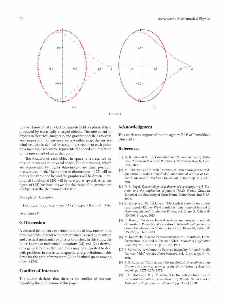
Weyl-Euler-Lagrange Equations of Motion on Flat Manifold Zeki KasapVolume 2015 Article ID 808016 11 pages
On Finsler Geometry and Applications in Mechanics Review and New Perspectives J D ClaytonVolume 2015 Article ID 828475 11 pages
A Variational Approach to Electrostatics of Polarizable Heterogeneous Substances Michael Grinfeld andPavel GrinfeldVolume 2015 Article ID 659127 7 pages
Comparison of Optimal Homotopy Asymptotic and Adomian Decomposition Methods for aThin FilmFlow of aThird Grade Fluid on a Moving Belt Fazle Mabood and Nopparat PochaiVolume 2015 Article ID 642835 4 pages
EditorialMechanics and Geometry of Solids and Surfaces
J D Clayton12 M A Grinfeld1 T Hasebe3 and J R Mayeur4
1 Impact Physics US ARL Aberdeen MD 21005-5066 USA2A James Clark School (Adjunct) University of Maryland College Park MD 20742 USA3Department of Mechanical Engineering Kobe University Kobe 657-8501 Japan4Theoretical Division Los Alamos National Laboratory Los Alamos NM 87545 USA
Correspondence should be addressed to J D Clayton johndclayton1civmailmil
Received 5 June 2015 Accepted 2 July 2015
Copyright copy 2015 J D Clayton et al This is an open access article distributed under the Creative Commons Attribution Licensewhich permits unrestricted use distribution and reproduction in any medium provided the original work is properly cited
1 Introduction
Invited were overview and original research papers ontopics associated with mechanics and geometry of solidsand surfaces Contributors have diverse backgrounds ina number of technical disciplines including theoreticaland mathematical physics pure and applied mathematicsengineering mechanics or materials science Submissionsoriginating from North America Europe and Asia werereceived and peer-reviewed over a period of approximatelyone calendar year spanning June 2014ndashJune 2015 Invitedresearch topics included butwere not limited to the followingcontinuum physics and mechanics of materials includingnonlinear elasticity plasticity and higher-order gradient ormicropolar theory [1] mechanics and thermodynamics ofmoving surfaces [2] including phase transition fronts andshock waves materials physics of crystal lattices glassesand interfaces in heterogeneous solids multiphysics [3] andmultiscale modeling differential-geometric descriptions asapplied to condensed matter physics and nonlinear science[4] theory and new analytical solutions or new applicationsof existing solutions to related problems in mechanicsphysics and geometry new developments in numericalmethods of solution towards mechanics problems and newphysical experiments supporting or suggesting new theo-retical descriptions Published papers are grouped into fourcategories in what follows wherein the content and relevanceof each contribution are summarized These categories arekinematicsgeometry of surfaces (Section 2) electrostatics(Section 3) solid mechanics (Section 4) and thermal-fluidmechanics (Section 5)
2 KinematicsGeometry of Surfaces
In ldquoTheRelationship between Focal Surfaces and Surfaces at aConstantDistance from the Edge of Regression on a Surfacerdquothe coauthors S Yurttancikmaz and O Tarakci investigatethe relationship between focal surfaces and surfaces at aconstant distance from the edge of regression on a surfaceThey show how focal surfaces of a manifold can be obtainedby means of some special surfaces at a constant distancefrom the edge of regression on the manifold Focal surfacesare known in the topic of line congruence which has beenintroduced in the general field of visualization Applicationsinclude visualization of the pressure and heat distributionson an airplane and studies of temperature rainfall or ozoneover the earthrsquos surface Focal surfaces are also used as aninterrogation tool to analyze the quality of various structuresbefore further processing in industrial settings for examplein numerical controlled milling operations
In ldquoWeyl-Euler-Lagrange Equations of Motion on FlatManifoldrdquo the author Z Kasap studies Weyl-Euler-Lagrangeequations ofmotion in a flat space It is well known that a Rie-mannian manifold is flat if its curvature is everywhere zeroFurthermore a flat manifold is one Euclidean space in termsof distances Weyl introduced a metric with a conformaltransformation for unified theory in 1918 Classicalmechanicsproblems are often analyzed via the Euler-Lagrange equa-tions In this study partial differential equations are obtainedfor movement of objects in space and solutions of theseequations are generated using symbolic algebra softwareThepresent set of Euler-Lagrange mechanical equations derivedon a generalization of flat manifolds may be suggested to deal
Hindawi Publishing CorporationAdvances in Mathematical PhysicsVolume 2015 Article ID 382083 3 pageshttpdxdoiorg1011552015382083
2 Advances in Mathematical Physics
with problems in electricalmagnetic and gravitational fieldsfor the paths of defined space-moving objects
In ldquoThe Steiner Formula and the Polar Moment of Inertiafor the Closed Planar Homothetic Motions in ComplexPlanerdquo the coauthors A Tutar and O Sener express theSteiner area formula and the polar moment of inertia duringone-parameter closed planar homothetic motions in thecomplex plane The Steiner point or Steiner normal conceptsare described according to whether a rotation number isdifferent from zero or equal to zero respectively The movingpole point is given with its components and its relationbetween a Steiner point and a Steiner normal is specifiedThesagittal motion of a winch is considered as an example Thismotion is described by a double hinge consisting of the fixedcontrol panel of the winch and its moving arm The winchis studied here because its arm can extend or retract duringone-parameter closed planar homothetic motions
3 Electrostatics
In ldquoA Variational Approach to Electrostatics of PolarizableHeterogeneous Substancesrdquo the coauthors M Grinfeld andP Grinfeld discuss equilibrium conditions for heterogeneoussubstances subject to electrostatic or magnetostatic effectsThe goal of this paper is to present a logically consistentextension of the Gibbs variational approach [2] to elasticbodies with interfaces in the presence of electromagneticeffects It is demonstrated that the force-like aleph tensorand the energy-like beth tensor for polarizable deformablesubstances are divergence-free Two additional tensors areintroduced the divergence-free energy-like gimel tensorfor rigid dielectrics and the general electrostatic gammatensor which is not necessarily divergence-free The presentapproach is based on a logically consistent extension of theGibbs energy principle that takes into account polarizationeffects
Contrary to many prior attempts explicitly excluded arethe electric field and the electric displacement from the list ofindependent thermodynamic variables Instead polarizationis treated by adding a single term to the traditional free energyfor a thermoelastic systemThe additional term represents thepotential energy accumulated in the electrostatic field overthe entire space The exact nonlinear theory of continuousmedia is invoked with Eulerian coordinates as the indepen-dent spatial variables
While the proposed model is mathematically rigorousthe authors caution against the assumption that it can reliablypredict physical phenomena On the contrary clear modelsoften lead to conclusions at odds with experiment andtherefore should be treated as physical paradoxes that deservethe attention of the scientific community
4 Solid Mechanics
In ldquoOn Finsler Geometry and Applications in MechanicsReview and New Perspectivesrdquo the author J D Claytonbegins with a review of necessary mathematical definitionsand derivations and then reviews prior work involvingapplication of Finsler geometry in continuum mechanics of
solids The use of Finsler geometry (eg [5]) to describecontinuum mechanical behavior of solids was suggestednearly five decades ago by Kroner in 1968 [1] As overlookedin the initial review by the author Finsler geometry wasapplied towards deforming ferromagnetic crystals by Amariin 1962 [3] and has somewhat recently been applied to frac-ture mechanics problems [6] Building on theoretical workof Ikeda [7] Bejancu [8] distinguished among horizontaland vertical distributions of the fiber bundle of a finite-deforming pseudo-Finslerian total space More completetheories incorporating a Lagrangian functional (leading tophysical balance or conservation laws) and couched in termsof Finsler geometry were developed by Stumpf and Saczukfor describing inelasticity mechanisms such as plasticity anddamage [9] including the only known published solutions ofboundary value problems incorporating such sophistication
This contributed paper by J D Clayton also introducesaspects of a new theoretical description of mechanics ofcontinua with microstructure This original theory thoughneither complete nor fully explored combines ideas fromfinite deformation kinematics [10] Finsler geometry [5 8]and phase field theories of materials physics Future work willenable encapsulation of phase field modeling of fracture andpossible electromechanical couplingwithin Finsler geometricframework
5 Thermal-Fluid Mechanics
In ldquoComparison of Optimal Homotopy Asymptotic andAdomian Decomposition Methods for a Thin Film Flow ofa Third Grade Fluid on a Moving Beltrdquo the coauthors FMabood and N Pochai investigate a thin film flow of athird-grade fluid on a moving belt using a powerful andrelatively new approximate analytical technique known asthe Optimal Homotopy Asymptotic Method (OHAM) Dueto model complexities difficulties often arise in obtainingsolutions of governing nonlinear differential equations fornon-Newtonian fluids A second-grade fluid is one of themost acceptable fluids in this class because of its mathemati-cal simplicity in comparison to third-grade and fourth-gradefluids In related literature many authors have effectivelytreated the complicated nonlinear equations governing theflow of a third-grade fluid In this study it is observedthat the OHAM is a powerful approximate analytical toolthat is simple and straightforward and does not requirethe existence of any small or large parameter as does thetraditional perturbationmethodThe variation of the velocityprofile for different parameters is compared with numericalvalues obtained by the Runge-Kutta-Fehlberg fourth-fifth-ordermethod andwith theAdomianDecompositionMethod(ADM) An interesting result of the analysis is that the three-term OHAM solution is more accurate than five-term ADMsolution confirming feasibility of the former method
In ldquoOptimalHomotopyAsymptotic Solution for Exother-mic Reactions Model with Constant Heat Source in a PorousMediumrdquo the coauthors F Mabood and N Pochai consideranalytical and numerical treatments of heat transfer inparticular problems Heat flow patternsprofiles are requiredfor heat transfer simulation in various types of thermal
Advances in Mathematical Physics 3
insulationThe exothermic reactionmodels for porousmediacan often be prescribed in the form of sets of nonlinearordinary differential equations In this research the drivingforce model due to temperature gradients is considered Agoverning equation of the model is restructured into anenergy balance equation that provides the temperature profilein a conduction state with a constant heat source in thesteady state A proposed Optimal Homotopy AsymptoticMethod (OHAM) is used to compute the solutions of theexothermic reactions equations The posited OHAM schemeis convenient to implement has fourth-order accuracy anddemonstrates no obvious problematic instabilities
J D ClaytonM A Grinfeld
T HasebeJ R Mayeur
References
[1] E Kroner ldquoInterrelations between various branches of con-tinuum mechanicsrdquo in Mechanics of Generalized Continua EKroner Ed pp 330ndash340 Springer Berlin Germany 1968
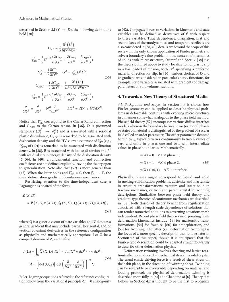
[2] M A Grinfeld Thermodynamic Methods in the Theory ofHeterogeneous Systems Longman Sussex UK 1991
[3] S Amari ldquoA theory of deformations and stresses of ferromag-netic substances by Finsler geometryrdquo in RAAG Memoirs KKondo Ed vol 3 pp 257ndash278 1962
[4] J D Clayton Nonlinear Mechanics of Crystals Springer Dor-drecht The Netherlands 2011
[5] H Rund The Differential Geometry of Finsler Spaces SpringerBerlin Germany 1959
[6] I A Miklashevich ldquoGeometric characteristics of fracture-associated space and crack propagation in a materialrdquo Journalof Applied Mechanics and Technical Physics vol 44 no 2 pp255ndash261 2003
[7] S Ikeda ldquoA physico-geometrical consideration on the theoryof directors in the continuum mechanics of oriented mediardquoTensor New Series vol 27 pp 361ndash368 1973
[8] A Bejancu Finsler Geometry and Applications Ellis HorwoodNew York NY USA 1990
[9] H Stumpf and J Saczuk ldquoA generalized model of oriented con-tinuum with defectsrdquo Zeitschrift fur Angewandte Mathematikund Mechanik vol 80 no 3 pp 147ndash169 2000
[10] J D ClaytonDifferential Geometry and Kinematics of ContinuaWorld Scientific Singapore 2014
Research ArticleThe Relationship between Focal Surfaces and Surfaces ata Constant Distance from the Edge of Regression on a Surface
Semra Yurttancikmaz and Omer Tarakci
Department of Mathematics Faculty of Science Ataturk University 25240 Erzurum Turkey
Correspondence should be addressed to Semra Yurttancikmaz semrakayaatauniedutr
Received 7 July 2014 Accepted 8 September 2014
Academic Editor John D Clayton
Copyright copy 2015 S Yurttancikmaz and O Tarakci This is an open access article distributed under the Creative CommonsAttribution License which permits unrestricted use distribution and reproduction in any medium provided the original work isproperly cited
We investigate the relationship between focal surfaces and surfaces at a constant distance from the edge of regression on a surfaceWe show that focal surfaces F
1and F
2of the surface M can be obtained by means of some special surfaces at a constant distance
from the edge of regression on the surfaceM
1 Introduction
Surfaces at a constant distance from the edge of regression ona surface were firstly defined by Tarakci in 2002 [1] Thesesurfaces were obtained by taking a surface instead of acurve in the study suggested by Hans Vogler in 1963 In thementioned study Hans Vogler asserted notion of curve at aconstant distance from the edge of regression on a curveAlso Tarakci and Hacisalihoglu calculated some propertiesand theorems which known for parallel surfaces for surfacesat a constant distance from the edge of regression on a surface[2] Later various authors became interested in surfaces at aconstant distance from the edge of regression on a surface andinvestigated Euler theorem and Dupin indicatrix conjugatetangent vectors and asymptotic directions for this surface [3]and examined surfaces at a constant distance from the edgeof regression on a surface in 1198643
1Minkowski space [4]
Another issue that we will use in this paper is the focalsurface Focal surfaces are known in the field of line con-gruence Line congruence has been introduced in the field ofvisualization by Hagen et al in 1991 [5] They can be used tovisualize the pressure and heat distribution on an airplanetemperature rainfall ozone over the earthrsquos surface andso forth Focal surfaces are also used as a surface interrogationtool to analyse the ldquoqualityrdquo of the surface before furtherprocessing of the surface for example in a NC-milling oper-ation [6] Generalized focal surfaces are related to hedgehog
diagrams Instead of drawing surface normals proportionalto a surface value only the point on the surface normalproportional to the function is drawing The loci of all thesepoints are the generalized focal surface This method wasintroduced byHagen andHahmann [6 7] and is based on theconcept of focal surface which is known from line geometryThe focal surfaces are the loci of all focal points of specialcongruence the normal congruence In later years focalsurfaces have been studied by various authors in differentfields
In this paper we have discovered a new method to con-stitute focal surfaces by means of surfaces at a constantdistance from the edge of regression on a surface Focalsurfaces 119865
1and 119865
2of the surface119872 in 1198643 are associated with
surfaces at a constant distance from the edge of regressionon 119872 that formed along directions of 119885
119875lying in planes
119878119901120601119906 119873 and 119878119901120601V 119873 respectively
2 Surfaces at a Constant Distance fromthe Edge of Regression on a Surface
Definition 1 Let119872 and119872119891 be two surfaces in 1198643 Euclideanspace and let 119873
119875be a unit normal vector and let 119879
119875119872 be
tangent space at point 119875 of surface 119872 and let 119883119875 119884119875 be
orthonormal bases of 119879119875119872 Take a unit vector 119885
119875= 1198891119883119875+
Hindawi Publishing CorporationAdvances in Mathematical PhysicsVolume 2015 Article ID 397126 6 pageshttpdxdoiorg1011552015397126
2 Advances in Mathematical Physics
1198892119884119875+1198893119873119875 where 119889
1 1198892 1198893isin R are constant and 1198892
1+1198892
2+
1198892
3= 1 If there is a function 119891 defined by
119891 119872 997888rarr 119872119891 119891 (119875) = 119875 + 119903119885
119875 (1)
where 119903 isin R then the surface 119872119891 is called the surface at aconstant distance from the edge of regression on the surface119872
Here if 1198891= 1198892= 0 then119885
119875= 119873119875and so119872 and119872119891 are
parallel surfaces Now we represent parametrization of sur-faces at a constant distance from the edge of regression on119872Let (120601 119880) be a parametrization of119872 so we can write that
120601 119880 sub 1198642997888rarr 119872
(119906 V) 120601 (119906 V) (2)
In case 120601119906 120601V is a basis of 119879
119875119872 then we can write that
119885119875= 1198891120601119906+1198892120601V+1198893119873119875 where120601119906 120601V are respectively partial
derivatives of 120601 according to 119906 and V Since 119872119891 = 119891(119875)
119891(119875) = 119875 + 119903119885119875 a parametric representation of119872119891 is
120595 (119906 V) = 120601 (119906 V) + 119903119885 (119906 V) (3)
Thus it is obtained that
119872119891= 120595 (119906 V) 120595 (119906 V)
= 120601 (119906 V)
+ 119903 (1198891120601119906(119906 V)
+ 1198892120601V (119906 V)
+ 1198893119873(119906 V))
(4)
and if we get 1199031198891= 1205821 1199031198892= 1205822 1199031198893= 1205823 then we have
119872119891= 120595 (119906 V) 120595 (119906 V)
= 120601 (119906 V) + 1205821120601119906(119906 V)
+ 1205822120601V (119906 V) + 1205823119873(119906 V)
1205822
1+ 1205822
2+ 1205822
3= 1199032
(5)
Calculation of 120595119906and 120595V gives us that
120595119906= 120601119906+ 1205821120601119906119906+ 1205822120601V119906 + 1205823119873119906
120595V = 120601V + 1205821120601119906V + 1205822120601VV + 1205823119873V(6)
Here 120601119906119906 120601V119906 120601119906V 120601VV 119873119906 119873V are calculated as in [1] We
choose curvature lines instead of parameter curves of119872 andlet 119906 and V be arc length of these curvature lines Thus thefollowing equations are obtained
120601119906119906= minus 120581
1119873
120601VV = minus 1205812119873
120601119906V = 120601V119906 = 0
119873119906= 1205811120601119906
119873V = 1205812120601V
(7)
From (6) and (7) we find
120595119906= (1 + 120582
31205811) 120601119906minus 12058211205811119873
120595V = (1 + 12058231205812) 120601V minus 12058221205812119873
(8)
and 120595119906 120595V is a basis of 120594(119872119891) If we denote by 119873119891 unit
normal vector of119872119891 then119873119891 is
119873119891=
[120595119906 120595V]
1003817100381710038171003817[120595119906 120595V]1003817100381710038171003817
= (12058211205811(1 + 120582
31205812) 120601119906+ 12058221205812(1 + 120582
31205811) 120601V
+ (1 + 12058231205811) (1 + 120582
31205812)119873)
times (1205822
11205812
1(1 + 120582
31205812)2
+ 1205822
21205812
2(1 + 120582
31205811)2
+ (1 + 12058231205811)2
(1 + 12058231205812)2
)minus12
(9)
where 1205811 1205812are principal curvatures of the surface119872 If
119860 = (1205822
11205812
1(1 + 120582
31205812)2
+ 1205822
21205812
2(1 + 120582
31205811)2
+(1 + 12058231205811)2
(1 + 12058231205812)2
)12
(10)
we can write
119873119891=12058211205811(1 + 120582
31205812)
119860120601119906+12058221205812(1 + 120582
31205811)
119860120601V
+(1 + 120582
31205811) (1 + 120582
31205812)
119860119873
(11)
Here in case of 1205811= 1205812and 120582
3= minus1120581
1= minus1120581
2since120595
119906and
120595V are not linearly independent119872119891 is not a regular surface
We will not consider this case [1]
3 Focal Surfaces
The differential geometry of smooth three-dimensional sur-faces can be interpreted from one of two perspectives interms of oriented frames located on the surface or in termsof a pair of associated focal surfaces These focal surfacesare swept by the loci of the principal curvatures radiiConsidering fundamental facts from differential geometry itis obvious that the centers of curvature of the normal sectioncurves at a particular point on the surface fill out a certainsegment of the normal vector at this pointThe extremities ofthese segments are the centers of curvature of two principaldirections These two points are called the focal points ofthis particular normal [8] This terminology is justified bythe fact that a line congruence can be considered as theset of lines touching two surfaces the focal surfaces of theline congruence The points of contact between a line of thecongruence and the two focal surfaces are the focal pointsof this line It turns out that the focal points of a normalcongruence are the centers of curvature of the two principaldirections [9 10]
Advances in Mathematical Physics 3
We represent surfaces parametrically as vector-valuedfunctions 120601(119906 V) Given a set of unit vectors 119885(119906 V) a linecongruence is defined
119862 (119906 V) = 120601 (119906 V) + 119863 (119906 V) 119885 (119906 V) (12)
where 119863(119906 V) is called the signed distance between 120601(119906 V)and 119885(119906 V) [8] Let 119873(119906 V) be unit normal vector of thesurface If 119885(119906 V) = 119873(119906 V) then 119862 = 119862
119873is a normal
congruence A focal surface is a special normal congruenceThe parametric representation of the focal surfaces of 119862
119873is
given by
119865119894(119906 V) = 120601 (119906 V) minus
1
120581119894(119906 V)
119873 (119906 V) 119894 = 1 2 (13)
where 1205811 1205812are the principal curvatures Except for parabolic
points and planar points where one or both principal curva-tures are zero each point on the base surface is associatedwith two focal points Thus generally a smooth base surfacehas two focal surface sheets 119865
1(119906 V) and 119865
2(119906 V) [11]
The generalization of this classical concept leads to thegeneralized focal surfaces
119865 (119906 V) = 120601 (119906 V) + 119886119891 (1205811 1205812)119873 (119906 V) with 119886 isin R (14)
where the scalar function 119891 depends on the principal curva-tures 120581
1= 1205811(119906 V) and 120581
2= 1205812(119906 V) of the surface119872The real
number 119886 is used as a scale factor If the curvatures are verysmall you need a very large number 119886 to distinguish the twosurfaces 120601(119906 V) and 119865(119906 V) on the screen Variation of thisfactor can also improve the visibility of several properties ofthe focal surface for example one can get intersectionsclearer [6]
4 The Relationship between Focal Surfacesand Surfaces at a Constant Distance fromthe Edge of Regression on a Surface
Theorem 2 Let surface 119872 be given by parametrical 120601(119906 V)One considers all surfaces at a constant distance from the edgeof regression on 119872 that formed along directions of 119885
119875lying
in plane 119878119901120601119906 119873 Normals of these surfaces at points 119891(119875)
corresponding to point 119875 isin 119872 generate a spatial family of lineof which top is center of first principal curvature 119862
1= 119875minus
(11205811(119875))119873
119875at 119875
Proof Surfaces at a constant distance from the edge of reg-ression on 119872 that formed along directions of 119885
119875lying in
plane 119878119901120601119906 119873 are defined by
119891119894 119872 997888rarr 119872
119891119894 119894 = 1 2
119891119894(119875) = 119875 + 120582
1119894120601119906(119875) + 120582
3119894119873119875
(15)
These surfaces and their unit normal vectors are respectivelydenoted by119872119891119894 and 119873119891119894 We will demonstrate that intersec-tion point of lines which pass from the point 119891
119894(119875) and are in
direction119873119891119894119891119894(119875)
is 1198621= 119875 minus (1120581
1(119875))119873
119875
The normal vector of the surface119872119891119894 at the point 119891119894(119875) is
119873119891119894 = 120582
11198941205811(119875) 120601119906(119875) + (1 + 120582
31198941205811(119875))119873
119875 (16)
Here it is clear that 119873119891119894 is in plane 119878119901120601119906 119873 Suppose that
line passing from the point119891119894(119875) and being in direction119873119891119894
119891119894(119875)
is 119889119894and a representative point of 119889
119894is119876 = (119909 119910) = 119909120601
119906(119875) +
119910119873119875 then the equation of 119889
119894is
119889119894sdot sdot sdot
997888997888rarr119875119876 =
997888997888997888997888997888rarr119875119891119894(119875) + 120583
1119873119891119894
119891119894(119875) (17)
Besides suppose that line passing from the point 119891119895(119875) and
being in direction119873119891119895119891119895(119875)
is 119889119895and a representative point of 119889
119895
is 119877 = (119909 119910) then equation of 119889119895is
119889119895sdot sdot sdot
997888rarr119875119877 =
997888997888997888997888997888rarr119875119891119895(119875) + 120583
2119873119891119895
119891119895(119875) 119895 = 1 2 (18)
We find intersection point of these lines Since it is studiedin plane of vectors 120601
119906(119875)119873
119875 the point 119875 can be taken as
beginning point If we arrange the lines 119889119894and 119889
119895 then we
find
119889119894sdot sdot sdot (119909 119910) = (120582
1119894 1205823119894) + 1205831(12058211198941205811 1 + 120582
31198941205811)
119889119894sdot sdot sdot 119910 =
1 + 12058231198941205811
12058211198941205811
119909 minus1
1205811
119889119895sdot sdot sdot (119909 119910) = (120582
1119895 1205823119895) + 1205832(12058211198951205811 1 + 120582
31198951205811)
119889119895sdot sdot sdot 119910 =
1 + 12058231198951205811
12058211198951205811
119909 minus1
1205811
(19)
From here it is clear that intersection point of 119889119894and 119889
119895is
(119909 119910) = (0 minus11205811) So intersection point of the lines119889
119894and119889119895
is the point1198621= 119875minus(1120581
1(119875))119873
119875in plane 119878119901120601
119906(119875)119873
119875
Corollary 3 Directions of normals of all surfaces at a constantdistance from the edge of regression on 119872 that formed alongdirections of 119885
119875lying in plane 119878119901120601
119906 119873 intersect at a single
point This point 1198621= 119875 minus (1120581
1(119875))119873
119875which is referred in
Theorem 2 is on the focal surface 1198651
We know that
1198651(119875) = 119875 minus
1
1205811
119873119875 (20)
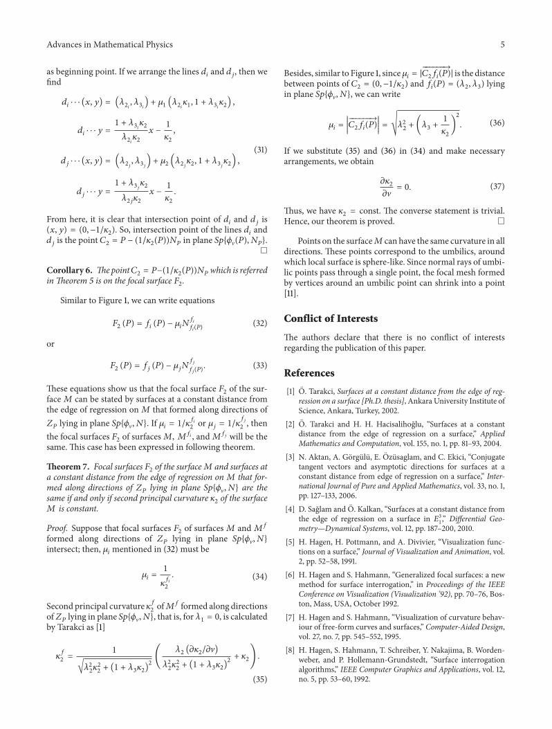
from definition of focal surfaces Moreover we can see easilythe following equations from Figure 1
1198651(119875) = 119891
119894(119875) minus 120583
119894119873119891119894
119891119894(119875)(21)
or
1198651(119875) = 119891
119895(119875) minus 120583
119895119873119891119895
119891119895(119875) (22)
These equations show us that the focal surface 1198651of the sur-
face119872 can be stated by surfaces at a constant distance from
4 Advances in Mathematical Physics
the edge of regression on119872 that formed along directions of119885119875lying in plane 119878119901120601
119906 119873 If 120583
119894= 1120581
119891119894
1or 120583119895= 1120581
119891119895
1 then
the focal surfaces 1198651of surfaces119872 119872
119891119894 and119872119891119895 will be thesame This case has been expressed in following theorem
Theorem 4 Focal surfaces 1198651of the surface119872 and surfaces at
a constant distance from the edge of regression on119872 that for-med along directions of 119885
119875lying in plane 119878119901120601
119906 119873 are the
same if and only if first principal curvature 1205811of the surface
119872 is constant
Proof Suppose that focal surfaces 1198651of surfaces119872 and119872119891
formed along directions of 119885119875
lying in plane 119878119901120601119906 119873
intersect then 120583119894mentioned in (21) must be
120583119894=
1
120581119891119894
1
(23)
First principal curvature 1205811198911of119872119891 formed along directions of
119885119875lying in plane 119878119901120601
119906 119873 that is for 120582
2= 0 is calculated
by Tarakci as [1]
120581119891
1=
1
radic1205822
11205812
1+ (1 + 120582
31205811)2
(1205821(1205971205811120597119906)
1205822
11205812
1+ (1 + 120582
31205811)2+ 1205811)
(24)
Besides from Figure 1 since 120583119894= |
997888997888997888997888997888997888rarr1198621119891119894(119875)| is distance bet-
ween points of 1198621= (0 minus1120581
1) and 119891
119894(119875) = (120582
1 1205823) lying in
plane 119878119901120601119906 119873 we can write
120583119894=
1003816100381610038161003816100381610038161003816
997888997888997888997888997888997888rarr1198621119891119894(119875)
1003816100381610038161003816100381610038161003816= radic1205822
1+ (1205823+1
1205811
)
2
(25)
If we substitute (24) and (25) in (23) and make necessaryarrangements we obtain
1205971205811
120597119906= 0 (26)
Thus we have 1205811= const The converse statement is trivial
Hence our theorem is proved
Theorem 5 Let surface 119872 be given by parametrical 120601(119906 V)We consider all surfaces at a constant distance from the edgeof regression on119872 that formed along directions of 119885
119875lying in
plane 119878119901120601V 119873 Normals of these surfaces at points 119891(119875)corresponding to point 119875 isin 119872 generate a spatial family of lineof which top is center of second principal curvature 119862
2= 119875minus
(11205812(119875))119873
119875at 119875
Proof Surfaces at a constant distance from the edge of regre-ssion on119872 that formed along directions of 119885
119875lying in plane
119878119901120601V 119873 are defined by
119891119894 119872 997888rarr 119872
119891119894 119894 = 1 2
119891119894(119875) = 119875 + 120582
2119894120601V (119875) + 1205823119894119873119875
(27)
M
F1
dj
di
C1 = F1(P)
P 120601u
NPZP119894
ZP119895
fi(P)
fj(P)
Nf119894
Nf119895Mf119894
Mf119895
1
1205811
Figure 1 Directions of normals of all surfaces at a constant distancefrom the edge of regression on119872 that formed along directions of119885
119875
lying in plane 119878119901120601119906 119873 and their intersection point (focal point)
These surfaces and their unit normal vectors are respectivelydenoted by119872119891119894 and 119873119891119894 We will demonstrate that intersec-tion point of lines which pass from the point 119891
119894(119875) and are in
direction119873119891119894119891119894(119875)
is 1198622= 119875 minus (1120581
2(119875))119873
119875
The normal vector of the surface119872119891119894 at the point 119891119894(119875) is
119873119891119894 = 120582
21198941205812(119875) 120601V (119875) + (1 + 12058231198941205812 (119875))119873119875 (28)
Here it is clear that 119873119891119894 is in plane 119878119901120601V 119873 Suppose thatline passing from the point119891
119894(119875) and being in direction119873119891119894
119891119894(119875)
is 119889119894and a representative point of 119889
119894is 119876 = (119909 119910) = 119909120601V(119875) +
119910119873119875 then equation of 119889
119894is
119889119894sdot sdot sdot
997888997888rarr119875119876 =
997888997888997888997888997888rarr119875119891119894(119875) + 120583
1119873119891119894
119891119894(119875) (29)
Besides suppose that line passing from the point 119891119895(119875) of the
surface119872119891119895 and being in direction119873119891119895119891119895(119875)
is119889119895and a represen-
tative point of 119889119895is 119877 = (119909 119910) then equation of 119889
119895is
119889119895sdot sdot sdot
997888rarr119875119877 =
997888997888997888997888997888rarr119875119891119895(119875) + 120583
2119873119891119895
119891119895(119875) 119895 = 1 2 (30)
We find intersection point of these two lines Since it is stud-ied in plane of vectors 120601V(119875)119873119875 the point 119875 can be taken
Advances in Mathematical Physics 5
as beginning point If we arrange the lines 119889119894and 119889
119895 then we
find
119889119894sdot sdot sdot (119909 119910) = (120582
2119894 1205823119894) + 1205831(12058221198941205811 1 + 120582
31198941205812)
119889119894sdot sdot sdot 119910 =
1 + 12058231198941205812
12058221198941205812
119909 minus1
1205812
119889119895sdot sdot sdot (119909 119910) = (120582
2119895 1205823119895) + 1205832(12058221198951205812 1 + 120582
31198951205812)
119889119895sdot sdot sdot 119910 =
1 + 12058231198951205812
12058221198951205812
119909 minus1
1205812
(31)
From here it is clear that intersection point of 119889119894and 119889
119895is
(119909 119910) = (0 minus11205812) So intersection point of the lines 119889
119894and
119889119895is the point 119862
2= 119875 minus (1120581
2(119875))119873
119875in plane 119878119901120601V(119875)119873119875
Corollary 6 Thepoint1198622= 119875minus(1120581
2(119875))119873
119875which is referred
in Theorem 5 is on the focal surface 1198652
Similar to Figure 1 we can write equations
1198652(119875) = 119891
119894(119875) minus 120583
119894119873119891119894
119891119894(119875)(32)
or
1198652(119875) = 119891
119895(119875) minus 120583
119895119873119891119895
119891119895(119875) (33)
These equations show us that the focal surface 1198652of the sur-
face119872 can be stated by surfaces at a constant distance fromthe edge of regression on119872 that formed along directions of119885119875lying in plane 119878119901120601V 119873 If 120583119894 = 1120581
119891119894
2or 120583119895= 1120581
119891119895
2 then
the focal surfaces 1198652of surfaces119872 119872
119891119894 and119872119891119895 will be thesame This case has been expressed in following theorem
Theorem 7 Focal surfaces 1198652of the surface119872 and surfaces at
a constant distance from the edge of regression on119872 that for-med along directions of 119885
119875lying in plane 119878119901120601V 119873 are the
same if and only if second principal curvature 1205812of the surface
119872 is constant
Proof Suppose that focal surfaces 1198652of surfaces119872 and119872119891
formed along directions of 119885119875
lying in plane 119878119901120601V 119873
intersect then 120583119894mentioned in (32) must be
120583119894=
1
120581119891119894
2
(34)
Second principal curvature 1205811198912of119872119891 formed along directions
of119885119875lying in plane 119878119901120601V 119873 that is for 1205821 = 0 is calculated
by Tarakci as [1]
120581119891
2=
1
radic1205822
21205812
2+ (1 + 120582
31205812)2
(1205822(1205971205812120597V)
1205822
21205812
2+ (1 + 120582
31205812)2+ 1205812)
(35)
Besides similar to Figure 1 since120583119894= |997888997888997888997888997888997888rarr1198622119891119894(119875)| is the distance
between points of 1198622= (0 minus1120581
2) and 119891
119894(119875) = (120582
2 1205823) lying
in plane 119878119901120601V 119873 we can write
120583119894=
1003816100381610038161003816100381610038161003816
997888997888997888997888997888997888rarr1198622119891119894(119875)
1003816100381610038161003816100381610038161003816= radic1205822
2+ (1205823+1
1205812
)
2
(36)
If we substitute (35) and (36) in (34) and make necessaryarrangements we obtain
1205971205812
120597V= 0 (37)
Thus we have 1205812= const The converse statement is trivial
Hence our theorem is proved
Points on the surface119872 can have the same curvature in alldirections These points correspond to the umbilics aroundwhich local surface is sphere-like Since normal rays of umbi-lic points pass through a single point the focal mesh formedby vertices around an umbilic point can shrink into a point[11]
Conflict of Interests
The authors declare that there is no conflict of interestsregarding the publication of this paper
References
[1] O Tarakci Surfaces at a constant distance from the edge of reg-ression on a surface [PhD thesis] Ankara University Institute ofScience Ankara Turkey 2002
[2] O Tarakci and H H Hacisalihoglu ldquoSurfaces at a constantdistance from the edge of regression on a surfacerdquo AppliedMathematics and Computation vol 155 no 1 pp 81ndash93 2004
[3] N Aktan A Gorgulu E Ozusaglam and C Ekici ldquoConjugatetangent vectors and asymptotic directions for surfaces at aconstant distance from edge of regression on a surfacerdquo Inter-national Journal of Pure and Applied Mathematics vol 33 no 1pp 127ndash133 2006
[4] D Saglam and O Kalkan ldquoSurfaces at a constant distance fromthe edge of regression on a surface in 119864
3
1rdquo Differential Geo-
metrymdashDynamical Systems vol 12 pp 187ndash200 2010[5] H Hagen H Pottmann and A Divivier ldquoVisualization func-
tions on a surfacerdquo Journal of Visualization and Animation vol2 pp 52ndash58 1991
[6] H Hagen and S Hahmann ldquoGeneralized focal surfaces a newmethod for surface interrogationrdquo in Proceedings of the IEEEConference on Visualization (Visualization rsquo92) pp 70ndash76 Bos-ton Mass USA October 1992
[7] H Hagen and S Hahmann ldquoVisualization of curvature behav-iour of free-form curves and surfacesrdquo Computer-Aided Designvol 27 no 7 pp 545ndash552 1995
[8] H Hagen S Hahmann T Schreiber Y Nakajima B Worden-weber and P Hollemann-Grundstedt ldquoSurface interrogationalgorithmsrdquo IEEE Computer Graphics and Applications vol 12no 5 pp 53ndash60 1992
6 Advances in Mathematical Physics
[9] J Hoschek Linien-Geometrie BI Wissensehaffs Zurich Swit-zerland 1971
[10] K StrubeckerDifferentialgeometrie III DeGruyter Berlin Ger-many 1959
[11] J Yu X Yin X Gu L McMillan and S Gortler ldquoFocal Surfacesof discrete geometryrdquo in Eurographics Symposium on GeometryProcessing 2007
Research ArticleThe Steiner Formula and the Polar Moment of Inertia for theClosed Planar Homothetic Motions in Complex Plane
Ayhan Tutar and Onder Sener
Department of Mathematics Ondokuz Mayis University Kurupelit 55139 Samsun Turkey
Correspondence should be addressed to Ayhan Tutar atutaromuedutr
Received 29 December 2014 Accepted 23 February 2015
Academic Editor John D Clayton
Copyright copy 2015 A Tutar and O Sener This is an open access article distributed under the Creative Commons AttributionLicense which permits unrestricted use distribution and reproduction in any medium provided the original work is properlycited
The Steiner area formula and the polar moment of inertia were expressed during one-parameter closed planar homothetic motionsin complex planeThe Steiner point or Steiner normal concepts were described according to whether rotation number was differentfrom zero or equal to zero respectivelyThemoving pole point was given with its components and its relation between Steiner pointor Steiner normalwas specifiedThe sagittalmotion of awinchwas considered as an exampleThismotionwas described by a doublehinge consisting of the fixed control panel of winch and the moving arm of winch The results obtained in the second section ofthis study were applied for this motion
1 Introduction
For a geometrical object rolling on a line and making acomplete turn some properties of the area of a path of a pointwere given by [1] The Steiner area formula and the Holditchtheorem during one-parameter closed planar homotheticmotions were expressed by [2] We calculated the expressionof the Steiner formula relative to the moving coordinate sys-tem under one-parameter closed planar homothetic motionsin complex plane If the points of the moving plane whichenclose the same area lie on a circle then the centre of thiscircle is called the Steiner point (ℎ = 1) [3 4] If thesepoints lie on a line we use Steiner normal instead of SteinerpointThen we obtained the moving pole point for the closedplanar homothetic motions We dealt with the polar momentof inertia of a path generated by a closed planar homotheticmotion Furthermore we expressed the relation between thearea enclosed by a path and the polar moment of inertia Asan example the sagittal motion of a winch which is describedby a double hinge being fixed and moving was consideredThe Steiner area formula the moving pole point and thepolar moment of inertia were calculated for this motionMoreover the relation between the Steiner formula and thepolar moment of inertia was expressed
2 Closed Homothetic Motions inComplex Plane
We consider one-parameter closed planar homotheticmotion between two reference systems the fixed 119864
1015840 andthe moving 119864 with their origins (119874 119874
1015840) and orientations in
complex planeThen we take into account motion relative tothe fixed coordinate system (direct motion)
By taking displacement vectors 1198741198741015840= 119880 and 119874
1015840119874 = 119880
1015840
and the total angle of rotation 120572(119905) the motion defined by thetransformation
1198831015840(119905) = ℎ (119905)119883119890
119894120572(119905)+ 1198801015840(119905) (1)
is called one-parameter closed planar homotheticmotion anddenoted by 1198641198641015840 where ℎ is a homothetic scale of the motion1198641198641015840 and119883 and1198831015840 are the position vectors with respect to the
moving and fixed rectangular coordinate systems of a point119883 isin 119864 respectively The homothetic scale ℎ and the vectors1198831015840 and 119880119880
1015840 are continuously differentiable functions of areal parameter 119905
In (1) 1198831015840(119905) is the trajectory with respect to the fixedsystem of a point 119883 belonging to the moving system If wereplace 1198801015840 = minus119880119890
119894120572(119905) in (1) the motion can be written as
1198831015840(119905) = (ℎ (119905)119883 minus 119880 (119905)) 119890
119894120572(119905) (2)
Hindawi Publishing CorporationAdvances in Mathematical PhysicsVolume 2015 Article ID 978294 5 pageshttpdxdoiorg1011552015978294
2 Advances in Mathematical Physics
The coordinates of the above equation are
1198831015840(119905) = 119909
1015840
1(119905) + 119894119909
1015840
2(119905) 119880
1015840(119905) = 119906
1015840
1(119905) + 119894119906
1015840
2(119905)
119883 = 1199091+ 1198941199092 119880 (119905) = 119906
1(119905) + 119894119906
2(119905)
(3)
Using these coordinates we can write
1199091015840
1(119905) + 119894119909
1015840
2(119905) = [(ℎ (119905) 119909
1minus 1199061) + 119894 (ℎ (119905) 119909
2minus 1199062)]
sdot (cos120572 (119905) + 119894 sin120572 (119905))
(4)
From (4) the components of1198831015840(119905)may be given as
1199091015840
1(119905) = cos (120572 (119905)) (ℎ (119905) 119909
1minus 1199061) minus sin (120572 (119905)) (ℎ (119905) 119909
2minus 1199062)
1199091015840
2(119905) = sin (120572 (119905)) (ℎ (119905) 119909
1minus 1199061) + cos (120572 (119905)) (ℎ (119905) 119909
2minus 1199062)
(5)
Using the coordinates of (2) as
1198831015840(119905) = (
1199091015840
1(119905)
1199091015840
2(119905)
) 1198801015840(119905) = (
1199061015840
1(119905)
1199061015840
2(119905)
)
119883 = (
1199091
1199092
) 119880 (119905) = (
1199061(119905)
1199062(119905)
)
(6)
and rotation matrix
119877 (119905) = (
cos (120572 (119905)) minus sin (120572 (119905))
sin (120572 (119905)) cos (120572 (119905))) (7)
we can obtain
1198831015840(119905) = 119877 (119905) (ℎ (119905)119883 minus 119880 (119905)) (8)
If we differentiate (5) we have
1198891199091015840
1= minus sin120572 (ℎ119909
1minus 1199061) 119889120572 + cos120572 (119889ℎ119909
1minus 1198891199061)
minus cos120572 (ℎ1199092minus 1199062) 119889120572 minus sin120572 (119889ℎ119909
2minus 1198891199062)
1198891199091015840
2= cos120572 (ℎ119909
1minus 1199061) 119889120572 + sin120572 (119889ℎ119909
1minus 1198891199061)
minus sin120572 (ℎ1199092minus 1199062) 119889120572 + cos120572 (119889ℎ119909
2minus 1198891199062)
(9)
21 The Steiner Formula for the Homothetic Motions Theformula for the area 119865 of a closed planar curve of the point1198831015840 is given by
119865 =1
2∮(1199091015840
11198891199091015840
2minus 1199091015840
21198891199091015840
1) (10)
If (5) and (9) are placed in (10) we have
2119865 = (1199092
1+ 1199092
2)∮ℎ2119889120572 + 119909
1∮(minus2ℎ119906
1119889120572 minus ℎ119889119906
2+ 1199062119889ℎ)
+ 1199092∮(minus2ℎ119906
2119889120572 + ℎ119889119906
1minus 1199061119889ℎ)
+ ∮(1199062
1+ 1199062
2) 119889120572 + 119906
11198891199062minus 11990621198891199061
(11)
The following expressions are used in (11)
∮(minus2ℎ1199061119889120572 minus ℎ119889119906
2+ 1199062119889ℎ) = 119886
lowast
∮ (minus2ℎ1199062119889120572 + ℎ119889119906
1minus 1199061119889ℎ) = 119887
lowast
∮ (1199062
1+ 1199062
2) 119889120572 + 119906
11198891199062minus 11990621198891199061 = 119888
(12)
The scalar term 119888 which is related to the trajectory of theorigin of themoving systemmay be given as follows by taking119865119900= 119865 (119909
1= 0 119909
2= 0)
2119865119900= 119888 (13)
The coefficient119898
119898 = ∮ℎ2119889120572 = ℎ
2(1199050)∮119889120572 = ℎ
2(1199050) 2120587] (14)
with the rotation number ] determines whether the lines with119865 = const describe circles or straight lines If ] = 0 then wehave circles If ] = 0 the circles reduce to straight lines If (12)(13) and (14) are substituted in (11) then
2 (119865 minus 119865119900) = (119909
2
1+ 1199092
2)119898 + 119886
lowast1199091+ 119887lowast1199092
(15)
can be obtained
211 A Different Parametrization for the Integral CoefficientsEquation (8) by differentiation with respect to 119905 yields
1198891198831015840= 119889119877 (ℎ119883 minus 119880) + 119877 (119889ℎ119883 minus 119889119880) (16)
If119883 = 119875 = (11990111199012) (the pole point) is taken
0 = 1198891198831015840= 119889119877 (ℎ119875 minus 119880) + 119877 (119889ℎ119875 minus 119889119880) (17)
can be written Then if 119880 = (11990611199062) is solved from (17)
1199061= ℎ1199011+ 1199012
119889ℎ
119889120572minus1198891199062
119889120572
1199062= ℎ1199012minus 1199011
119889ℎ
119889120572+1198891199061
119889120572
(18)
are foundIf (18) is placed in (12)
119886lowast= ∮(minus2ℎ
21199011119889120572) + ∮ (minus2ℎ119889ℎ119901
2+ ℎ119889119906
2+ 1199062119889ℎ)
119887lowast= ∮(minus2ℎ
21199012119889120572) + ∮ (2ℎ119889ℎ119901
1minus ℎ119889119906
1minus 1199061119889ℎ)
(19)
can be rewritten Also (19) can be expressed separately as
119886 = ∮ (minus2ℎ21199011119889120572) 119887 = ∮ (minus2ℎ
21199012119889120572) (20)
1205831= ∮ (minus2ℎ119889ℎ119901
2+ ℎ119889119906
2+ 1199062119889ℎ)
1205832= ∮ (2ℎ119889ℎ119901
1minus ℎ119889119906
1minus 1199061119889ℎ)
120583 = (
1205831
1205832
)
(21)
Advances in Mathematical Physics 3
Using (20) and (21) the area formula
2 (119865 minus 119865119900) = (119909
2
1+ 1199092
2)119898 + 119886119909
1+ 1198871199092+ 12058311199091+ 12058321199092
(22)
is found
22 Steiner Point or Steiner Normal for the HomotheticMotions By taking 119898 = 0 the Steiner point 119878 = (119904
1 1199042) for
the closed planar homothetic motion can be written
119904119895=
∮ℎ2119901119895119889120572
∮ℎ2119889120572
119895 = 1 2 (23)
Then
∮ℎ21199011119889120572 = 119904
1119898 ∮ℎ
21199012119889120572 = 119904
2119898 (24)
is found If (24) is placed in (20) and by considering (22)
2 (119865 minus 119865119900) = 119898 (119909
2
1+ 1199092
2minus 211990411199091minus 211990421199092) + 12058311199091+ 12058321199092
(25)
is obtained Equation (25) is called the Steiner area formulafor the closed planar homothetic motion
By dividing this by119898 and by completing the squares oneobtains the equation of a circle
(1199091minus (1199041minus
1205831
2119898))
2
+ (1199092minus (1199042minus
1205832
2119898))
2
minus (1199041minus
1205831
2119898)
2
minus (1199042minus
1205832
2119898)
2
=2 (119865 minus 119865
0)
119898
(26)
All the fixed points of the moving plane which pass aroundequal orbit areas under themotion119864119864
1015840 lie on the same circlewith the center
119872 = (1199041minus
1205831
2119898 1199042minus
1205832
2119898) (27)
in the moving planeIn the case of ℎ(119905) = 1 since 120583
1= 1205832= 0 the point 119872
and the Steiner point 119878 coincide [3] Also by taking 119898 = 0 ifit is replaced in (22) then we have
(119886 + 1205831) 1199091+ (119887 + 120583
2) 1199092minus 2 (119865 minus 119865
0) = 0 (28)
Equation (28) is a straight line If no complete loop occursthen 120578 = 0 and the circles are reduced to straight linesin other words to a circle whose center lies at infinity Thenormal to the lines of equal areas in (28) is given by
119899 = (
119886 + 1205831
119887 + 1205832
) (29)
which is called the Steiner normal [5]
23TheMoving Pole Point for the Homothetic Motions Using(18) if 119875 = (
11990111199012) is solved then the pole point 119875 of the motion
1199011=
119889ℎ (1198891199061minus 1199062119889120572) + ℎ119889120572 (119889119906
2+ 1199061119889120572)
(119889ℎ)2+ ℎ2 (119889120572)
2
1199012=
119889ℎ (1198891199062+ 1199061119889120572) minus ℎ119889120572 (119889119906
1minus 1199062119889120572)
(119889ℎ)2+ ℎ2 (119889120572)
2
(30)
is obtainedFor119898 = 0 using (14) and (23) we arrive at the relation in
(24) between the Steiner point and the pole pointFor 119898 = 0 using (20) and (29) we arrive at the relation
between the Steiner normal and the pole point as follows
(
119886
119887) = (
minus2∮ℎ21199011119889120572
minus2∮ℎ21199012119889120572
) = 119899 minus 120583 (31)
24 The Polar Moments of Inertia for the Homothetic MotionsThe polar moments of inertia ldquo119879rdquo symbolize a path for closedhomothetic motions We find a formula by using 119879119898 and 119899
in this section and we arrive at the relation between the polarmoments of inertia ldquo119879rdquo and the formula of area ldquo119865rdquo (see (37))A relation between the Steiner formula and the polarmomentof inertia around the pole for a moment was given by [6]Muller [3] also demonstrated a relation to the polar momentof inertia around the origin while Tolke [7] inspected thesame relation for closed functions and Kuruoglu et al [8]generalized Mullerrsquos results for homothetic motion
If we use 120572 as a parameter we need to calculate
119879 = ∮(1199091015840
1
2
+ 1199091015840
2
2
) 119889120572 (32)
along the path of119883 Then using (5)
119879 = (1199092
1+ 1199092
2)119898 + 119909
1∮(minus2ℎ119906
1119889120572)
+ 1199092∮(minus2ℎ119906
2119889120572) + ∮(119906
2
1+ 1199062
2) 119889120572
(33)
is obtainedWe need to calculate the polar moments of inertia of the
origin of the moving system therefore 119879119900= 119879 (119909
1= 0 119909
2=
0) one obtains
119879119900= ∮(119906
2
1+ 1199062
2) 119889120572 (34)
If (34) is placed in (33)
119879 minus 119879119900= (1199092
1+ 1199092
2)119898 + 119909
1∮(minus2ℎ119906
1119889120572) + 119909
2∮(minus2ℎ119906
2119889120572)
(35)
can be written Also if (18) is placed in (35)
119879 minus 119879119900= (1199092
1+ 1199092
2)119898 + 119909
1∮(minus2ℎ
21199011119889120572 minus 2ℎ119889ℎ119901
2+ 2ℎ119889119906
2)
+ 1199092∮(minus2ℎ
21199012119889120572 + 2ℎ119889ℎ119901
1minus 2ℎ119889119906
1)
(36)
4 Advances in Mathematical Physics
x1
x2
x9984001
x9984002
L
k
120001
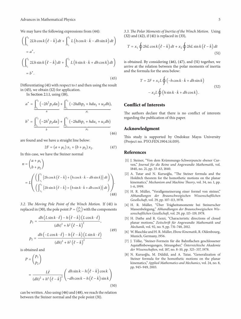
Figure 1 The arms of winch as a double hinge
is obtained and by considering (22) and (36) together wearrive at the relation between the polar moments of inertiaand the formula for the area below
119879 minus 119879119900= 2 (119865 minus 119865
119900) + 1199091∮(ℎ119889119906
2minus 1199062119889ℎ)
+ 1199092∮(minusℎ119889119906
1+ 1199061119889ℎ)
(37)
3 Application The Motion of the Winch
In the previous sections we emphasized three conceptsgeometrical objects as the Steiner point or the Steiner normalthe pole point and the polar moments of inertia for closedhomothetic motions in complex plane In this section wewant to visualize the experimentally measured motion withthese objects Accordingly we consider these characteristicdirections for this motion
We will show how the kinematical objects which areused in the previous sections can be applied In the study byDathe and Gezzi [5] they considered human gait in planarmotions As an example we have chosen the sagittal part ofthe movement of the winch at motion We have chosen thewinch because the arm of winch can extend or retract duringone-parameter closed planar homotheticmotionThemotionof winch has a double hinge and ldquoa double hingerdquo means thatit has two systems a fixed arm and a moving arm of winch(Figure 1) There is a control panel of winch at the origin offixed system ldquo119871rdquo arm can extend or retract by ℎ parameter
31 The Mathematical Model We start by writing the equa-tions of the double hinge in Cartesian coordinates Then wedefine using the condition119898 = 0 the Steiner normal and thetotal angle in relation to the double hinge
By taking displacement vectors 1198741198741015840= 119880 and 119874
1015840119874 = 119880
1015840
and the total angle of rotation 119897 minus 119896 = 120572 the motion can bedefined by the transformation
1198831015840(119905) = ℎ (119905)119883119890
119894(119897(119905)minus119896(119905))+ 1198801015840(119905) (38)
By taking
119877 (119905) = (
cos (ℓ (119905) minus 119896 (119905)) minus sin (ℓ (119905) minus 119896 (119905))
sin (ℓ (119905) minus 119896 (119905)) cos (ℓ (119905) minus 119896 (119905)))
1198801015840(119905) = (
119871 cos (ℓ (119905))119871 sin (ℓ (119905))
)
(39)
we have
1198831015840(119905) = ℎ (119905) 119877 (119905)119883 + 119880
1015840(119905) (40)
Also we know that 1198801015840 = minus119877119880 Therefore
119880 (119905) = (
1199061(119905)
1199062(119905)
) = (
minus119871 cos (119896 (119905))minus119871 sin (119896 (119905))
) (41)
can be written So the double hinge may be written as
1199091015840
1(119905) = cos (ℓ (119905) minus 119896 (119905)) (ℎ (119905) 119909
1+ 119871 cos (119896))
minus sin (ℓ (119905) minus 119896 (119905)) (ℎ (119905) 1199092+ 119871 sin (119896))
1199091015840
2(119905) = sin (ℓ (119905) minus 119896 (119905)) (ℎ (119905) 119909
1+ 119871 cos (119896))
+ cos (ℓ (119905) minus 119896 (119905)) (ℎ (119905) 1199092+ 119871 sin (119896))
(42)
We begin by calculating the time derivative of (42) In thisway we obtain the velocities
1199091015840
1(119905)
1199091015840
2(119905) which have to be
inserted into (10)
1199091015840
1
1199091015840
2minus 1199091015840
2
1199091015840
1
= (ℎ2(1199092
1+ 1199092
2) + 1198712) ( ℓ (119905) minus 119896(119905))
+ 1199091(2ℎ119871 cos (119896 (119905)) ( ℓ (119905) minus 119896(119905))
+ ℎ119871 cos (119896 (119905)) 119896 (119905) minus 119871119889ℎ sin (119896 (119905)))
+ 1199092(2ℎ119871 sin (119896 (119905)) ( ℓ (119905) minus 119896(119905))
+ ℎ119871 sin (119896 (119905)) 119896 (119905) + 119871119889ℎ cos (119896 (119905)))
+ 1198712 119896(119905)
(43)
We now integrate the previous equation using periodicboundary conditions by assuming the integrands as periodicfunctions The periodicity of 119891 implies that integrals of thefollowing types vanish ∮119889119891 = int
119865
1
119891119889119905 = 119891|119865
1= 0 As a result
of this some of the integrals of (43) are not equal to zero andwe finally obtain a simplified expression for the area
2119865 = 1199091(int
1199052
1199051
2119871ℎ cos 119896 ( ℓ minus 119896)119889119905
+int
1199052
1199051
119871 (ℎ cos 119896 sdot 119896 minus 119889ℎ sin 119896) 119889119905)
+ 1199092(int
1199052
1199051
2119871ℎ sin 119896 ( ℓ minus 119896)119889119905
+int
1199052
1199051
119871 (ℎ sin 119896 sdot 119896 + 119889ℎ cos 119896) 119889119905)
(44)
Advances in Mathematical Physics 5
We may have the following expressions from (44)
(int
1199052
1199051
2119871ℎ cos 119896 ( ℓ minus 119896)119889119905 + int
1199052
1199051
119871 (ℎ cos 119896 sdot 119896 minus 119889ℎ sin 119896) 119889119905)
= 119886lowast
(int
1199052
1199051
2119871ℎ sin 119896 ( ℓ minus 119896)119889119905 + int
1199052
1199051
119871 (ℎ sin 119896 sdot 119896 + 119889ℎ cos 119896) 119889119905)
= 119887lowast
(45)
Differentiating (41) with respect to 119905 and then using the resultin (45) we obtain (12) for application
In Section 211 using (18)
119886lowast= int
1199052
1199051
(minus2ℎ21199011119889120572)
⏟⏟⏟⏟⏟⏟⏟⏟⏟⏟⏟⏟⏟⏟⏟⏟⏟⏟⏟⏟⏟⏟⏟⏟⏟⏟⏟⏟⏟
119886
+ int
1199052
1199051
(minus2ℎ119889ℎ1199012+ ℎ119889119906
2+ 1199062119889ℎ)
⏟⏟⏟⏟⏟⏟⏟⏟⏟⏟⏟⏟⏟⏟⏟⏟⏟⏟⏟⏟⏟⏟⏟⏟⏟⏟⏟⏟⏟⏟⏟⏟⏟⏟⏟⏟⏟⏟⏟⏟⏟⏟⏟⏟⏟⏟⏟⏟⏟⏟⏟⏟⏟⏟⏟⏟⏟
1205831
119887lowast= int
1199052
1199051
(minus2ℎ21199012119889120572)
⏟⏟⏟⏟⏟⏟⏟⏟⏟⏟⏟⏟⏟⏟⏟⏟⏟⏟⏟⏟⏟⏟⏟⏟⏟⏟⏟⏟⏟
119887
+ int
1199052
1199051
(minus2ℎ119889ℎ1199011+ ℎ119889119906
1+ 1199061119889ℎ)
⏟⏟⏟⏟⏟⏟⏟⏟⏟⏟⏟⏟⏟⏟⏟⏟⏟⏟⏟⏟⏟⏟⏟⏟⏟⏟⏟⏟⏟⏟⏟⏟⏟⏟⏟⏟⏟⏟⏟⏟⏟⏟⏟⏟⏟⏟⏟⏟⏟⏟⏟⏟⏟⏟⏟⏟⏟
1205832
(46)
are found and we have a straight line below
2119865 = (119886 + 1205831) 1199091+ (119887 + 120583
2) 1199092 (47)
In this case we have the Steiner normal
119899 = (
119886 + 1205831
119887 + 1205832
)
= 119871(
(int
1199052
1199051
2ℎ cos 119896 ( ℓ minus 119896) + (ℎ cos 119896 sdot 119896 minus 119889ℎ sin 119896) 119889119905)
(int
1199052
1199051
2ℎ sin 119896 ( ℓ minus 119896) + (ℎ sin 119896 sdot 119896 + 119889ℎ cos 119896) 119889119905))
(48)
32 The Moving Pole Point of the Winch Motion If (41) isreplaced in (30) the pole point119875 = (
11990111199012)with the components
1199011=
119889ℎ (119871 sin 119896 sdot ℓ) minus ℎ ( ℓ minus 119896) (119871 cos 119896 sdot ℓ)
(119889ℎ)2+ ℎ2 ( ℓ minus 119896)
2
1199012=
119889ℎ (minus119871 cos 119896 sdot ℓ) minus ℎ ( ℓ minus 119896) (119871 sin 119896 sdot ℓ)
(119889ℎ)2+ ℎ2 ( ℓ minus 119896)
2
(49)
is obtained and
119875 = (
1199011
1199012
)
=119871 ℓ
(119889ℎ)2+ ℎ2 ( ℓ minus 119896)
2(
119889ℎ sin 119896 minus ℎ ( ℓ minus 119896) cos 119896
minus119889ℎ cos 119896 minus ℎ ( ℓ minus 119896) sin 119896
)
(50)
can be written Also using (46) and (48) we reach the relationbetween the Steiner normal and the pole point (31)
33The Polar Moments of Inertia of theWinchMotion Using(32) and (42) if (41) is replaced in (33)
119879 = 1199091∮2ℎ119871 cos 119896 ( ℓ minus 119896)119889119905 + 119909
2∮2ℎ119871 sin 119896 ( ℓ minus 119896)119889119905
(51)
is obtained By considering (46) (47) and (51) together wearrive at the relation between the polar moments of inertiaand the formula for the area below
119879 = 2119865 + 1199091119871∮(minusℎ cos 119896 sdot 119896 + 119889ℎ sin 119896)
minus 1199092119871∮(ℎ sin 119896 sdot 119896 + 119889ℎ cos 119896)
(52)
Conflict of Interests
The authors declare that there is no conflict of interestsregarding the publication of this paper
Acknowledgment
This study is supported by Ondokuz Mayıs University(Project no PYOFEN190414019)
References
[1] J Steiner ldquoVon dem Krummungs-Schwerpuncte ebener Cur-venrdquo Journal fur die Reine und Angewandte Mathematik vol1840 no 21 pp 33ndash63 1840
[2] A Tutar and N Kuruoglu ldquoThe Steiner formula and theHolditch theorem for the homothetic motions on the planarkinematicsrdquoMechanism and Machine Theory vol 34 no 1 pp1ndash6 1999
[3] H R Muller ldquoVerallgemeinerung einer formel von steinerrdquoAbhandlungen der Braunschweigischen WissenschaftlichenGesellschaft vol 29 pp 107ndash113 1978
[4] H R Muller ldquoUber Tragheitsmomente bei SteinerscherMassenbelegungrdquo Abhandlungen der Braunschweigischen Wis-senschaftlichen Gesellschaft vol 29 pp 115ndash119 1978
[5] H Dathe and R Gezzi ldquoCharacteristic directions of closedplanar motionsrdquo Zeitschrift fur Angewandte Mathematik undMechanik vol 92 no 9 pp 731ndash748 2012
[6] W Blaschke andH RMuller Ebene Kinematik R OldenbourgMunich Germany 1956
[7] J Tolke ldquoSteiner-Formein fur die Bahnflachen geschlossenerAquiaffinbewegungen Sitzungsberrdquo Osterreichische Akademieder Wissenschaften vol 187 no 8ndash10 pp 325ndash337 1978
[8] N Kuruoglu M Duldul and A Tutar ldquoGeneralization ofSteiner formula for the homothetic motions on the planarkinematicsrdquo Applied Mathematics and Mechanics vol 24 no 8pp 945ndash949 2003
Research ArticleOptimal Homotopy Asymptotic Solution forExothermic Reactions Model with Constant Heat Source ina Porous Medium
Fazle Mabood1 and Nopparat Pochai23
1Department of Mathematics University of Peshawar Peshawar Pakistan2Department of Mathematics King Mongkutrsquos Institute of Technology Ladkrabang Bangkok 10520 Thailand3Centre of Excellence in Mathematics CHE Si Ayutthaya Road Bangkok 10400 Thailand
Correspondence should be addressed to Nopparat Pochai nop mathyahoocom
Received 27 May 2015 Accepted 7 June 2015
Academic Editor John D Clayton
Copyright copy 2015 F Mabood and N Pochai This is an open access article distributed under the Creative Commons AttributionLicense which permits unrestricted use distribution and reproduction in any medium provided the original work is properlycited
The heat flow patterns profiles are required for heat transfer simulation in each type of the thermal insulation The exothermicreaction models in porous medium can prescribe the problems in the form of nonlinear ordinary differential equations In thisresearch the driving force model due to the temperature gradients is considered A governing equation of the model is restrictedinto an energy balance equation that provides the temperature profile in conduction state with constant heat source on the steadystate The proposed optimal homotopy asymptotic method (OHAM) is used to compute the solutions of the exothermic reactionsequation
1 Introduction
In physical systems energy is obtained from chemical bondsIf bonds are broken energy is needed If bonds are formedenergy is released Each type of bond has specific bondenergy It can be predictedwhether a chemical reactionwouldrelease or need heat by using bond energies If there is moreenergy used to form the bonds than to break the bonds heatis given offThis is well known as an exothermic reaction Onthe other hand if a reaction needs an input of energy it is saidto be an endothermic reaction The ability to break bonds isactivated energy
Convection has obtained growth uses in many areas suchas solar energy conversion underground coal gasificationgeothermal energy extraction ground water contaminanttransport and oil reservoir simulationThe exothermic reac-tionmodel is focused on the system inwhich the driving forcewas due to the applied temperature gradients at the boundaryof the system In [1ndash4] they proposed the investigationof Rayleigh-Bernard-type convection They also study theconvective instabilities that arise due to exothermic reactions
model in a porous mediumThe exothermic reactions releasethe heat create density differences within the fluid andinduce natural convection that turn out the rate of reactionaffects [5] The nonuniform flow of convective motion that isgenerated by heat sources is investigated by [6ndash8] In [9ndash13]they propose the two- and three-dimensional models ofnatural convection among different types of porous medium
In this research the optimal homotopy asymptoticmethod for conduction solutions is proposed The modelequation is a steady-state energy balance equation of thetemperature profile in conduction state with constant heatsource
The optimal homotopy asymptotic method is an approx-imate analytical tool that is simple and straightforward anddoes not require the existence of any small or large parameteras does traditional perturbation method As observed byHerisanu and Marinca [14] the most significant featureOHAM is the optimal control of the convergence of solu-tions via a particular convergence-control function 119867 andthis ensures a very fast convergence when its components(known as convergence-control parameters) are optimally
Hindawi Publishing CorporationAdvances in Mathematical PhysicsVolume 2015 Article ID 825683 4 pageshttpdxdoiorg1011552015825683
2 Advances in Mathematical Physics
determined In the recent paper of Herisanu et al [15] wherethe authors focused on nonlinear dynamical model of apermanent magnet synchronous generator in their studya different way of construction of homotopy is developedto ensure the fast convergence of the OHAM solutionsto the exact one Optimal Homotopy Asymptotic Method(OHAM) has been successfully been applied to linear andnonlinear problems [16 17] This paper is organized asfollows First in Section 2 exothermic reaction model ispresented In Section 3 we described the basic principlesof the optimal homotopy asymptotic method The optimalhomotopy asymptotic method solution of the problem isgiven in Section 4 Section 5 is devoted for the concludingremarks
2 Exothermic Reactions Model
In this section we introduce a pseudohomogeneous modelto express convective driven by an exothermic reaction Thecase of a porous medium wall thickness (0 lt 119911
1015840lt 119871)
is focused The normal assumption in the continuity andmomentum equations in the steady-state energy balancepresents a nondimensional formof a BVP for the temperatureprofile [5 13]
11988921205790
1198891199112+119861120601
2(1minus
1205790119861) exp(
1205741205790120574 + 1205790
) = 0 (1)
Here 1205790is the temperature the parameter 119861 is the maximum
feasible temperature in the absence of natural convection 1206012
is the ratio of the characteristic time for diffusion of heatgenerator and 120574 is the dimensionless activation energy In thecase of the constant heat source (1) can be written as
11988921205790
1198891199112+119861120601
2(1minus
1205790119861) = 0 (2)
subject to boundary condition
1198891205790119889119911
= 0 at 119911 = 0
1205790 = 0 at 119911 = 1(3)
3 Basic Principles of Optimal HomotopyAsymptotic Method
We review the basic principles of the optimal homotopyasymptotic method as follows
(i) Consider the following differential equation
119860 [119906 (119909)] + 119886 (119909) = 0 119909 isin Ω (4)
where Ω is problem domain 119860(119906) = 119871(119906) + 119873(119906) where 119871119873 are linear and nonlinear operators 119906(119909) is an unknownfunction and 119886(119909) is a known function
(ii) Construct an optimal homotopy equation as
(1minus119901) [119871 (120601 (119909 119901)) + 119886 (119909)]
minus119867 (119901) [119860 (120601 (119909 119901)) + 119886 (119909)] = 0(5)
where 0 le 119901 le 1 is an embedding parameter and119867(119901) = sum
119898
119894=1 119901119894119870119894is auxiliary function on which the con-
vergence of the solution greatly dependent Here 119870119895are
the convergence-control parameters The auxiliary function119867(119901) also adjusts the convergence domain and controls theconvergence region
(iii) Expand 120601(119909 119901 119870119895) in Taylorrsquos series about 119901 one has
an approximate solution
120601 (119909 119901 119870119895) = 1199060 (119909) +
infin
sum
119896=1119906119896(119909119870119895) 119901119896
119895 = 1 2 3
(6)
Many researchers have observed that the convergence of theseries equation (6) depends upon 119870
119895 (119895 = 1 2 119898) if it is
convergent then we obtain
V = V0 (119909) +119898
sum
119896=1V119896(119909119870119895) (7)
(iv) Substituting (7) in (4) we have the following residual
119877 (119909119870119895) = 119871 ( (119909 119870
119895)) + 119886 (119909) +119873( (119909119870
119895)) (8)
If119877(119909119870119895) = 0 then Vwill be the exact solution For nonlinear
problems generally this will not be the case For determining119870119895 (119895 = 1 2 119898) collocationmethod Ritz method or the
method of least squares can be used(v) Finally substituting the optimal values of the
convergence-control parameters 119870119895in (7) one can get the
approximate solution
4 Application of OHAM to an ExothermicReaction Model
Applying OHAM on (2) the zeroth first and second orderproblems are
(1minus119901) (12057910158401015840
0 ) minus119867 (119901) (12057910158401015840+119861120601
2(1minus
1205790119861)) = 0 (9)
We consider 1205790119867(119901) in the following manner
120579 = 12057900 +11990112057901 +119901212057902
1198671 (119901) = 1199011198701 +11990121198702
(10)
41 Zeroth Order Problem
12057910158401015840
00 = 0 (11)
with boundary conditions
12057900 (1) = 0
1205791015840
00 (0) = 0(12)
The solution of (11) with boundary condition (12) is
12057900 (119911) = 0 (13)
Advances in Mathematical Physics 3
42 First Order Problem
12057910158401015840
01 minus11987011206012119861 = 0 (14)
with boundary conditions
12057901 (1) = 0
1205791015840
01 (0) = 0(15)
The solution of (14) with boundary condition (15) is
12057901 (119911 1198701) =1198701120601
2119861
2(119911
2minus 1) (16)
43 Second Order Problem
12057910158401015840
02 (119911 1198701 1198702) = 11987011206012119861+119870
21120601
2119861minus
12119870
21120601
4119861119911
2
+12119870
21120601
4119861+
121198702120601
2119861
(17)
with boundary conditions
12057902 (1) = 0
1205791015840
02 (0) = 0(18)
The solution of (17) with boundary condition (18) is
12057902 (119911 1198701 1198702) =minus124
1206014119870
21119861119911
4+1212060121198701119861119911
2
+121206012119870
21119861119911
2+141206014119870
21119861119911
2
+1212060121198702119861119911
2minus
524
1206014119870
21119861
minus1212060121198701119861minus
121206012119870
21119861minus
1212060121198702119861
(19)
The final three terms solution via OHAM for 119901 = 1 is
1205790 (119911 1198701 1198702) = 12057900 (119911) + 12057901 (119911 1198701)
+ 12057902 (119911 1198701 1198702) (20)
The method of least squares is used to determine the con-vergence control parameters1198701 and1198702 in (20) In particularcase for 120601 = 1 119861 = 10 the values of the convergencecontrol parameters are 1198701 = minus08337205022 and 1198702 =
minus002092667470By substituting the values of 1198701 and 1198702 in (20) and after
simplification we can obtain the second order approximatesolution via OHAM To check the accuracy of the OHAMsolution a comparison between the solutions determined byOHAMandnumericalmethodswasmade and is presented inTable 1 Graphical representation of the solution using finitedifference technique [5] OHAM and Runge-Kutta Fehlbergfourth fifth order method is shown in Figure 1 an excellent
Table 1 Comparison of 1205790(119911) via OHAM and RKF45 for 120601 = 1 119861 =
10
119885 FDM [5] RKF45 OHAM Percentage error00 3114344 3518277 3518285 000022701 3046176 3485927 3485969 000120402 2911251 3388613 3388675 000182903 2711819 3225339 3225359 000062004 2451166 2994264 2994284 000066705 2133897 2693071 2693037 000126206 1766284 2318441 2318432 000038807 1356680 1866723 1866701 000117808 0915960 1333395 1333311 000629909 0457980 0713042 0713046 000056010 0000000 0000000 0000000 mdash
1 2 3 4 5 6 7 8 9 10 11
Tem
pera
ture
005
115
225
335
4
FDMRKF45OHAM
z
Figure 1 Comparison of analytical and numerical solution
agreement can be observedWe can see that the OHAM givesa better accurate solution than the traditional finite differencetechnique of [5] On the other hand the OHAM gives acontinuity solution but the traditional finite difference tech-nique gives a discrete solution It follows that the solutions ofthe OHAM is easier to implement than the finite differencesolutions
In Figure 2 we exhibit the effect of different values of 120601with fixed value of 119861 on temperature profile
5 Concluding Remarks
In this paper one has described an optimal homotopyasymptotic technique for obtaining the temperature profilesin porous medium We can see that the temperature reducesto the end The OHAM scheme for obtaining the model isconvenient to implement The OHAM gives fourth orderaccurate solutions It follows that the method has no insta-bility problem The model should be considered in the caseof nonconstant heat source
4 Advances in Mathematical Physics
0 02 04 06 08 10
1
2
3
4
51205790(z)
z
120601 = 1
120601 = 2
120601 = 3
120601 = 5
B = 5
Figure 2
Conflict of Interests
The authors declare that there is no conflict of interestsregarding the publication of this paper
Acknowledgments
This paper is supported by the Centre of Excellence inMathe-matics the Commission on Higher EducationThailandTheauthors greatly appreciate valuable comments received fromProfessor John D Clayton and their reviewers
References
[1] J L Beck ldquoConvection in a box of porous material saturatedwith fluidrdquo Physics of Fluids vol 15 no 8 pp 1377ndash1383 1972
[2] S HDavis ldquoConvection in a box linear theoryrdquo Journal of FluidMechanics vol 30 no 3 pp 465ndash478 1967
[3] Z Gershuni and E M Zhukovitskii Convective Stability ofIncompressible Fluids vol 4 Israel Program for ScientificTranslations 1976
[4] E R Lapwood ldquoConvection of a fluid in a porous mediumrdquoProceedings of the Cambridge Philosophical Society vol 44 pp508ndash521 1948
[5] N Pochai and J Jaisaardsuetrong ldquoA numerical treatment ofan exothermic reactions model with constant heat source ina porous medium using finite difference methodrdquo AdvancedStudies in Biology vol 4 no 6 pp 287ndash296 2012
[6] D R Jones ldquoThe dynamic stability of confined exothermicallyreacting fluidsrdquo International Journal of Heat andMass Transfervol 16 no 1 pp 157ndash167 1973
[7] M Tveitereid ldquoThermal convection in a horizontal porous layerwith internal heat sourcesrdquo International Journal of Heat andMass Transfer vol 20 no 10 pp 1045ndash1050 1977
[8] J B Bdzil andH L Frisch ldquoChemically driven convectionrdquoTheJournal of Chemical Physics vol 72 no 3 pp 1875ndash1886 1980
[9] H Viljoen and V Hlavacek ldquoChemically driven convection ina porous mediumrdquo AIChE Journal vol 33 no 8 pp 1344ndash13501987
[10] H J Viljoen J E Gatica and H Vladimir ldquoBifurcation analysisof chemically driven convectionrdquoChemical Engineering Sciencevol 45 no 2 pp 503ndash517 1990
[11] WW Farr J F Gabitto D Luss and V Balakotaiah ldquoReaction-driven convection in a porous mediumrdquo AIChE Journal vol 37no 7 pp 963ndash985 1991
[12] K Nandakumar and H J Weinitschke ldquoA bifurcation study ofchemically driven convection in a porous mediumrdquo ChemicalEngineering Science vol 47 no 15-16 pp 4107ndash4120 1992
[13] S Subramanian and V Balakotaiah ldquoConvective instabili-ties induced by exothermic reactions occurring in a porousmediumrdquo Physics of Fluids vol 6 no 9 pp 2907ndash2922 1994
[14] N Herisanu and V Marinca ldquoAccurate analytical solutions tooscillators with discontinuities and fractional-power restoringforce by means of the optimal homotopy asymptotic methodrdquoComputers amp Mathematics with Applications vol 60 no 6 pp1607ndash1615 2010
[15] N Herisanu V Marinca and G Madescu ldquoAn analyticalapproach to non-linear dynamical model of a permanentmagnet synchronous generatorrdquoWind Energy 2014
[16] F Mabood and N Pochai ldquoAsymptotic solution for a waterquality model in a uniform streamrdquo International Journal ofEngineering Mathematics vol 2013 Article ID 135140 4 pages2013
[17] V Marinca and N Herisanu ldquoOptimal homotopy perturbationmethod for strongly nonlinear differential equationsrdquoNonlinearScience Letters A vol 1 no 3 pp 273ndash280 2010
Research ArticleWeyl-Euler-Lagrange Equations of Motion on Flat Manifold
Zeki Kasap
Department of Elementary Education Faculty of Education Pamukkale University Kinikli Campus Denizli Turkey
Correspondence should be addressed to Zeki Kasap zekikasaphotmailcom
Received 27 April 2015 Accepted 11 May 2015
Academic Editor John D Clayton
Copyright copy 2015 Zeki Kasap This is an open access article distributed under the Creative Commons Attribution License whichpermits unrestricted use distribution and reproduction in any medium provided the original work is properly cited
This paper deals with Weyl-Euler-Lagrange equations of motion on flat manifold It is well known that a Riemannian manifold issaid to be flat if its curvature is everywhere zero Furthermore a flat manifold is one Euclidean space in terms of distances Weylintroduced a metric with a conformal transformation for unified theory in 1918 Classical mechanics is one of the major subfieldsof mechanics Also one way of solving problems in classical mechanics occurs with the help of the Euler-Lagrange equations Inthis study partial differential equations have been obtained for movement of objects in space and solutions of these equations havebeen generated by using the symbolic Algebra software Additionally the improvements obtained in this study will be presented
1 Introduction
Euler-Lagrangian (analogues) mechanics are very importanttools for differential geometry and analyticalmechanicsTheyhave a simple method to describe the model for mechanicalsystems The models for mechanical systems are relatedStudies in the literature about the Weyl manifolds are givenas follows Liu and Jun expand electronic origins moleculardynamics simulations computational nanomechanics andmultiscale modelling of materials fields [1] Tekkoyun andYayli examined generalized-quaternionic Kahlerian analogueof Lagrangian and Hamiltonian mechanical systems [2] Thestudy given in [3] has the particular purpose to examinethe discussion Weyl and Einstein had over Weylrsquos 1918 uni-fied field theory for reasons such as the epistemologicalimplications Kasap and Tekkoyun investigated Lagrangianand Hamiltonian formalism for mechanical systems usingpara-pseudo-Kahler manifolds representing an interestingmultidisciplinary field of research [4] Kasap obtained theWeyl-Euler-Lagrange and the Weyl-Hamilton equations onR2119899119899
which is a model of tangent manifolds of constant 119882-sectional curvature [5] Kapovich demonstrated an existencetheorem for flat conformal structures on finite-sheeted cov-erings over a wide class of Haken manifolds [6] Schwartzaccepted asymptotically Riemannian manifolds with non-negative scalar curvature [7] Kulkarni identified somenew examples of conformally flat manifolds [8] Dotti and
Miatello intend to find out the real cohomology ring of lowdimensional compact flat manifolds endowed with one ofthese special structures [9] Szczepanski presented a list of six-dimensional Kahler manifolds and he submitted an exampleof eight-dimensional Kahler manifold with finite group [10]Bartnik showed that the mass of an asymptotically flat 119899-manifold is a geometric invariant [11] Gonzalez consideredcomplete locally conformally flat metrics defined on adomain Ω sub 119878
119899 [12] Akbulut and Kalafat established infinitefamilies of nonsimply connected locally conformally flat(LCF) 4-manifold realizing rich topological types [13] Zhusuggested that it is to give a classification of complete locallyconformally flat manifolds of nonnegative Ricci curvature[14] Abood studied this tensor on general class almost Her-mitian manifold by using a newmethodology which is calledan adjoint 119866-structure space [15] K Olszak and Z Olszakproposed paraquaternionic analogy of these ideas applied toconformally flat almost pseudo-Kahlerian as well as almostpara-Kahlerian manifolds [16] Upadhyay studied boundingquestion for almost manifolds by looking at the equivalentdescription of them as infranil manifolds Γ 119871 ⋊ 119866119866 [17]
2 Preliminaries
Definition 1 With respect to tangent space given any point119901 isin 119872 it has a tangent space 119879
119901119872 isometric toR119899 If one has
a metric (inner-product) in this space ⟨ ⟩119901 119879119901119872times 119879
119901119872 997891rarr
Hindawi Publishing CorporationAdvances in Mathematical PhysicsVolume 2015 Article ID 808016 11 pageshttpdxdoiorg1011552015808016
2 Advances in Mathematical Physics
R defined on every point 119901 isin 119872119872 is called a Riemannianmanifold
Definition 2 A manifold with a Riemannian metric is a flatmanifold such that it has zero curvature
Definition 3 A differentiable manifold 119872 is said to be analmost complex manifold if there exists a linear map 119869
119879119872 rarr 119879119872 satisfying 1198692 = minus119894119889 and 119869 is said to be an almostcomplex structure of119872 where 119894 is the identity (unit) operatoron 119881 such that 119881 is the vector space and 1198692 = 119869 ∘ 119869
Theorem 4 The integrability of the almost complex structureimplies a relation in the curvature Let 1199091 1199101 1199092 1199102 1199093 1199103 becoordinates on R6 with the standard flat metric
1198891199042=
3sum
119894=1(119889119909
2119894+119889119910
2119894) (1)
(see [18])
Definition 5 A (pseudo-)Riemannian manifold is confor-mally flat manifold if each point has a neighborhood that canbe mapped to flat space by a conformal transformation Let(119872 119892) be a pseudo-Riemannian manifold
Theorem 6 Let (119872 119892) be conformally flat if for each point 119909in119872 there exists a neighborhood119880 of 119909 and a smooth function119891 defined on 119880 such that (119880 1198902119891119892) is flat The function 119891 neednot be defined on all of119872 Some authors use locally conformallyflat to describe the above notion and reserve conformally flat forthe case in which the function 119891 is defined on all of119872 [19]
Definition 7 A pseudo-119869-holomorphic curve is a smoothmap from a Riemannian surface into an almost complexmanifold such that it satisfies the Cauchy-Riemann equation[20]
Definition 8 A conformal map is a function which preservesangles as the most common case where the function isbetween domains in the complex plane Conformal maps canbe defined betweendomains in higher dimensional Euclideanspaces andmore generally on a (semi-)Riemannianmanifold
Definition 9 Conformal geometry is the study of the setof angle-preserving (conformal) transformations on a spaceIn two real dimensions conformal geometry is preciselythe geometry of Riemannian surfaces In more than twodimensions conformal geometry may refer either to thestudy of conformal transformations of flat spaces (such asEuclidean spaces or spheres) or to the study of conformalmanifolds which are Riemannian or pseudo-Riemannianmanifolds with a class of metrics defined up to scale
Definition 10 A conformal manifold is a differentiable mani-fold equippedwith an equivalence class of (pseudo-)Riemannmetric tensors in which two metrics 1198921015840 and 119892 are equivalentif and only if
1198921015840= Ψ
2119892 (2)
where Ψ gt 0 is a smooth positive function An equivalenceclass of such metrics is known as a conformal metric orconformal class and a manifold with a conformal structureis called a conformal manifold [21]
3 Weyl Geometry
Conformal transformation for use in curved lengths has beenrevealed The linear distance between two points can befound easily by Riemann metric Many scientists have usedthe Riemann metric Einstein was one of the first to studythis field Einstein discovered the Riemannian geometry andsuccessfully used it to describe general relativity in the 1910that is actually a classical theory for gravitation But theuniverse is really completely not like Riemannian geometryEach path between two points is not always linear Alsoorbits of moving objects may change during movement Soeach two points in space may not be linear geodesic Thena method is required for converting nonlinear distance tolinear distance Weyl introduced a metric with a conformaltransformation in 1918The basic concepts related to the topicare listed below [22ndash24]
Definition 11 Two Riemann metrics 1198921 and 1198922 on119872 are saidto be conformally equivalent iff there exists a smooth function119891 119872 rarr R with
1198901198911198921 = 1198922 (3)
In this case 1198921 sim 1198922
Definition 12 Let119872 be an 119899-dimensional smooth manifoldA pair (119872119866) where a conformal structure on 119872 is anequivalence class 119866 of Riemann metrics on 119872 is called aconformal structure
Theorem 13 Let nabla be a connection on119872 and 119892 isin 119866 a fixedmetric nabla is compatible with (119872119866) hArr there exists a 1-form 120596
with nabla119883119892 + 120596(119883)119892 = 0
Definition 14 A compatible torsion-free connection is calleda Weyl connection The triple (119872119866nabla) is a Weyl structure
Theorem 15 To each metric 119892 isin 119866 and 1-form 120596 there corre-sponds a unique Weyl connection nabla satisfying nabla
119883119892 +120596(119883)119892 =
0
Definition 16 Define a function 119865 1-forms on 119872 times 119866 rarr
Weyl connections by 119865(119892 120596) = nabla where nabla is the connec-tion guaranteed by Theorem 6 One says that nabla correspondsto (119892 120596)
Proposition 17 (1) 119865 is surjective
Proof 119865 is surjective byTheorem 13
(2) 119865(119892 120596) = 119865(119890119891119892 120578) iff 120578 = 120596 minus 119889119891 So
119865 (119890119891119892) = 119865 (119892) minus 119889119891 (4)
where 119866 is a conformal structure Note that a Riemann metric119892 and a one-form 120596 determine a Weyl structure namely 119865
Advances in Mathematical Physics 3
119866 rarr and1119872 where119866 is the equivalence class of 119892 and119865(119890119891119892) =
120596 minus 119889119891
Proof Suppose that 119865(119892 120596) = 119865(119890119891119892 120578) = nabla We have
nabla119883(119890119891119892) + 120578 (119883) 119890
119891119892
= 119883(119890119891) 119892 + 119890
119891nabla119883119892+ 120578 (119883) 119890
119891119892
= 119889119891 (119883) 119890119891119892+ 119890119891nabla119883119892+ 120578 (119883) 119890
119891119892 = 0
(5)
Thereforenabla119883119892 = minus(119889119891(119883)+120578(119883)) On the other handnabla
119883119892+
120596(119883)119892 = 0Therefore 120596 = 120578 + 119889119891 Set nabla = 119865(119892 120596) To shownabla = 119865(119890
119891119892 120578) and nabla
119883(119890119891119892) + 120578(119883)119890
119891119892 = 0 To calculate
nabla119883(119890119891119892) + 120578 (119883) 119890
119891119892
= 119890119891119889119891 (119883) 119892 + 119890
119891nabla119883119892+ (120596 (119883) minus 119889119891 (119883)) 119890
119891119892
= 119890119891(nabla119883119892+120596 (119883) 119892) = 0
(6)
Theorem 18 A connection on the metric bundle 120596 of aconformalmanifold119872naturally induces amap119865 119866 rarr and
1119872
and (4) and conversely Parallel translation of points in120596 by theconnection is the same as their translation by 119865
Theorem 19 Let nabla be a torsion-free connection on the tangentbundle of 119872 and 119898 ge 6 If (119872 119892 nabla 119869) is a Kahler-Weylstructure then the associated Weyl structure is trivial that isthere is a conformally equivalent metric 119892 = 119890
2119891119892 so that
(119872 119892 119869) is Kahler and so that nabla = nabla119892 [25ndash27]
Definition 20 Weyl curvature tensor is a measure of thecurvature of spacetime or a pseudo-Riemannian manifoldLike the Riemannian curvature tensor the Weyl tensorexpresses the tidal force that a body feels when moving alonga geodesic
Definition 21 Weyl transformation is a local rescaling ofthe metric tensor 119892
119886119887(119909) rarr 119890
minus2120596(119909)119892119886119887(119909) which produces
another metric in the same conformal class A theory oran expression invariant under this transformation is calledconformally invariant or is said to possess Weyl symmetryTheWeyl symmetry is an important symmetry in conformalfield theory
4 Complex Structures on ConformallyFlat Manifold
In this sectionWeyl structures on flatmanifoldswill be trans-ferred to the mechanical system Thus the time-dependentEuler-Lagrange partial equations of motion of the dynamicsystemwill be found A flatmanifold is something that locallylooks like Euclidean space in terms of distances and anglesThe basic example is Euclidean space with the usual metric119889119904
2= sum119894119889119909
2119894 Any point on a flat manifold has a neighbor-
hood isometric to a neighborhood in Euclidean space A flatmanifold is locally Euclidean in terms of distances and anglesand merely topologically locally Euclidean as all manifolds
are The simplest nontrivial examples occur as surfaces infour-dimensional space as the flat torus is a flat manifold Itis the image of 119891(119909 119910) = (cos119909 sin119909 cos119910 sin119910)
Example 22 It vanishes if and only if 119869 is an integrable almostcomplex structure that is given any point 119875 isin 119872 there existlocal coordinates (119909
119894 119910119894) 119894 = 1 2 3 centered at 119875 following
structures taken from
1198691205971199091 = cos (1199093) 1205971199101 + sin (1199093) 1205971199102
1198691205971199092 = minus sin (1199093) 1205971199101 + cos (1199093) 1205971199102
1198691205971199093 = 1205971199103
1198691205971199101 = minus cos (1199093) 1205971199091 + sin (1199093) 1205971199092
1198691205971199102 = minus sin (1199093) 1205971199091 minus cos (1199093) 1205971199092
1198691205971199103 = minus 1205971199093
(7)
The above structures (7) have been taken from [28] We willuse 120597119909
119894= 120597120597119909
119894and 120597119910
119894= 120597120597119910
119894
The Weyl tensor differs from the Riemannian curvaturetensor in that it does not convey information on how thevolume of the body changes In dimensions 2 and 3 theWeyl curvature tensor vanishes identically Also the Weylcurvature is generally nonzero for dimensions ge4 If theWeyltensor vanishes in dimension ge4 then the metric is locallyconformally flat there exists a local coordinate system inwhich the metric tensor is proportional to a constant tensorThis fact was a key component for gravitation and generalrelativity [29]
Proposition 23 If we extend (7) by means of conformalstructure [19 30] Theorem 19 and Definition 21 we can giveequations as follows
119869120597
1205971199091= 119890
2119891 cos (1199093)120597
1205971199101+ 119890
2119891 sin (1199093)120597
1205971199102
119869120597
1205971199092= minus 119890
2119891 sin (1199093)120597
1205971199101+ 119890
2119891 cos (1199093)120597
1205971199102
119869120597
1205971199093= 119890
2119891 120597
1205971199103
119869120597
1205971199101= minus 119890minus2119891 cos (1199093)
120597
1205971199091+ 119890minus2119891 sin (1199093)
120597
1205971199092
119869120597
1205971199102= minus 119890minus2119891 sin (1199093)
120597
1205971199091minus 119890minus2119891 cos (1199093)
120597
1205971199092
119869120597
1205971199103= minus 119890minus2119891 120597
1205971199093
(8)
such that they are base structures for Weyl-Euler-Lagrangeequations where 119869 is a conformal complex structure to be simi-lar to an integrable almost complex 119869 given in (7) Fromnow onwe continue our studies thinking of the (119879119872 119892 nabla 119869) instead of
4 Advances in Mathematical Physics
Weyl manifolds (119879119872 119892 nabla 119869) Now 119869 denotes the structure ofthe holomorphic property
1198692 120597
1205971199091= 119869 ∘ 119869
120597
1205971199091= 119890
2119891 cos (1199093) 119869120597
1205971199101+ 119890
2119891 sin (1199093) 119869
sdot120597
1205971199102= 119890
2119891 cos (1199093)
sdot [minus119890minus2119891 cos (1199093)
120597
1205971199091+ 119890minus2119891 sin (1199093)
120597
1205971199092]+ 119890
2119891
sdot sin (1199093) [minus119890minus2119891 sin (1199093)
120597
1205971199091minus 119890minus2119891 cos (1199093)
120597
1205971199092]
= minus cos2 (1199093)120597
1205971199091+ cos (1199093) sin (1199093)
120597
1205971199092
minus sin2 (1199093)120597
1205971199091minus sin (1199093) cos (1199093)
120597
1205971199092
= minus [cos2 (1199093) + sin2(1199093)]
120597
1205971199091= minus
120597
1205971199091
(9)
and in similar manner it is shown that
1198692 120597
120597119909119894
= minus120597
120597119909119894
1198692 120597
120597119910119894
= minus120597
120597119910119894
119894 = 1 2 3
(10)
As can be seen from (9) and (10) 1198692 = minus119868 are the complexstructures
5 Euler-Lagrange Dynamics Equations
Definition 24 (see [31ndash33]) Let119872 be an 119899-dimensional man-ifold and 119879119872 its tangent bundle with canonical projection120591119872 119879119872 rarr 119872 119879119872 is called the phase space of velocities of
the base manifold119872 Let 119871 119879119872 rarr R be a differentiablefunction on 119879119872 and it is called the Lagrangian function Weconsider closed 2-form on 119879119872 and Φ
119871= minus119889d
119869119871 Consider
the equation
i119881Φ119871= 119889119864119871 (11)
where the semispray 119881 is a vector field Also i is a reducingfunction and i
119881Φ119871= Φ119871(119881) We will see that for motion in
a potential 119864119871= V(119871) minus 119871 is an energy function (119871 = 119879minus119875 =
(12)119898V2 minus 119898119892ℎ kinetic-potential energies) and V = 119869119881
a Liouville vector field Here 119889119864119871denotes the differential
of 119864 We will see that (11) under a certain condition on 119881is the intrinsic expression of the Euler-Lagrange equationsof motion This equation is named Euler-Lagrange dynam-ical equation The triple (119879119872Φ
119871 119881) is known as Euler-
Lagrangian systemon the tangent bundle119879119872Theoperationsrun on (11) for any coordinate system (119902
119894(119905) 119901119894(119905)) Infinite
dimension Lagrangianrsquos equation is obtained in the formbelow
119889
119889119905(120597119871
120597 119902119894)minus
120597119871
120597119902119894= 0
119889119902119894
119889119905= 119902119894
119894 = 1 119899
(12)
6 Conformal Weyl-Euler-LagrangianEquations
Here we using (11) obtain Weyl-Euler-Lagrange equationsfor classical and quantum mechanics on conformally flatmanifold and it is shown by (119879119872 119892 nabla 119869)
Proposition 25 Let (119909119894 119910119894) be coordinate functions Also on
(119879119872 119892 nabla 119869) let 119881 be the vector field determined by 119881 =
sum3119894=1(119883119894(120597120597119909
119894) + 119884119894(120597120597119910119894)) Then the vector field defined by
V = 119869119881
= 1198831(119890
2119891 cos (1199093)120597
1205971199101+ 119890
2119891 sin (1199093)120597
1205971199102)
+1198832(minus119890
2119891 sin (1199093)120597
1205971199101+ 119890
2119891 cos (1199093)120597
1205971199102)
+11988331198902119891 120597
1205971199103
+1198841(minus119890minus2119891 cos (1199093)
120597
1205971199091+ 119890minus2119891 sin (1199093)
120597
1205971199092)
+1198842(minus119890minus2119891 sin (1199093)
120597
1205971199091minus 119890minus2119891 cos (1199093)
120597
1205971199092)
minus1198843119890minus2119891 120597
1205971199093
(13)
is thought to be Weyl-Liouville vector field on conformally flatmanifold (119879119872 119892 nabla 119869) Φ
119871= minus119889d
119869119871 is the closed 2-form
given by (11) such that d = sum3119894=1((120597120597119909119894)119889119909119894 + (120597120597119910119894)119889119910119894)
d119869 119865(119872) rarr and
1119872 d119869= 119894119869d minus d119894
119869 and d
119869= 119869(d) =
sum3119894=1(119883119894119869(120597120597119909
119894)+119884119894119869(120597120597119910
119894)) Also the vertical differentiation
d119869is given where 119889 is the usual exterior derivationThen there
is the following result We can obtain Weyl-Euler-Lagrangeequations for classical and quantummechanics on conformallyflat manifold (119879119872 119892 nabla 119869) We get the equations given by
d119869= [119890
2119891 cos (1199093)120597
1205971199101+ 119890
2119891 sin (1199093)120597
1205971199102] 1198891199091
+[minus1198902119891 sin (1199093)
120597
1205971199101+ 119890
2119891 cos (1199093)120597
1205971199102] 1198891199092
+ 1198902119891 120597
12059711991031198891199093
Advances in Mathematical Physics 5
+[minus119890minus2119891 cos (1199093)
120597
1205971199091+ 119890minus2119891 sin (1199093)
120597
1205971199092] 1198891199101
+[minus119890minus2119891 sin (1199093)
120597
1205971199091minus 119890minus2119891 cos (1199093)
120597
1205971199092] 1198891199102
minus 119890minus2119891 120597
12059711990931198891199103
(14)
Also
Φ119871= minus119889d
119869119871
= minus119889([1198902119891 cos (1199093)
120597
1205971199101+ 119890
2119891 sin (1199093)120597
1205971199102] 1198891199091
+[minus1198902119891 sin (1199093)
120597
1205971199101+ 119890
2119891 cos (1199093)120597
1205971199102] 1198891199092
+ 1198902119891 120597119871
12059711991031198891199093
+[minus119890minus2119891 cos (1199093)
120597
1205971199091+ 119890minus2119891 sin (1199093)
120597
1205971199092] 1198891199101
+[minus119890minus2119891 sin (1199093)
120597
1205971199091minus 119890minus2119891 cos (1199093)
120597
1205971199092] 1198891199102
minus 119890minus2119891 120597119871
12059711990931198891199103)
(15)
and then we find
i119881Φ119871= Φ119871(119881) = Φ
119871(
3sum
119894=1(119883119894 120597
120597119909119894
+119884119894 120597
120597119910119894
)) (16)
Moreover the energy function of system is
119864119871= 119883
1[119890
2119891 cos (1199093)120597119871
1205971199101+ 119890
2119891 sin (1199093)120597119871
1205971199102]
+1198832[minus119890
2119891 sin (1199093)120597119871
1205971199101+ 119890
2119891 cos (1199093)120597119871
1205971199102]
+11988331198902119891 120597119871
1205971199103
+1198841[minus119890minus2119891 cos (1199093)
120597119871
1205971199091+ 119890minus2119891 sin (1199093)
120597119871
1205971199092]
+1198842[minus119890minus2119891 sin (1199093)
120597119871
1205971199091minus 119890minus2119891 cos (1199093)
120597119871
1205971199092]
minus1198843119890minus2119891 120597119871
1205971199093minus119871
(17)
and the differential of 119864119871is
119889119864119871= 119883
1(119890
2119891 cos (1199093)1205972119871
120597119909112059711991011198891199091
+ 21198902119891 cos (1199093)120597119891
1205971199091
120597119871
12059711991011198891199091
+ 1198902119891 sin (1199093)
1205972119871
120597119909112059711991021198891199091
+ 21198902119891 sin (1199093)120597119891
1205971199091
120597119871
12059711991021198891199091)
+1198832(minus119890
2119891 sin (1199093)1205972119871
120597119909112059711991011198891199091
minus 21198902119891 sin (1199093)120597119891
1205971199091
120597119871
12059711991011198891199091
+ 1198902119891 cos (1199093)
1205972119871
120597119909112059711991021198891199091
+ 21198902119891 cos (1199093)120597119891
1205971199091
120597119871
12059711991021198891199091)
+1198833(119890
2119891 1205972119871
120597119909112059711991031198891199091 + 2119890
2119891 120597119891
1205971199091
120597119871
12059711991031198891199091)
+1198841(minus119890minus2119891 cos (1199093)
1205972119871
120597119909211198891199091
+ 2119890minus2119891 cos (1199093)120597119891
1205971199091
120597119871
12059711990911198891199091
+ 119890minus2119891 sin (1199093)
1205972119871
120597119909112059711990921198891199091
minus 2119890minus2119891 sin (1199093)120597119891
1205971199091
120597119871
12059711990921198891199091)
+1198842(minus119890minus2119891 sin (1199093)
1205972119871
120597119909211198891199091
+ 2119890minus2119891 sin (1199093)120597119891
1205971199091
120597119871
12059711990911198891199091
minus 119890minus2119891 cos (1199093)
1205972119871
120597119909112059711990921198891199091
+ 2119890minus2119891 cos (1199093)120597119891
1205971199091
120597119871
12059711990921198891199091)
+1198843(minus
1205972119871
120597119909112059711990931198891199091 + 2119890
minus2119891 120597119891
1205971199091
120597
12059711990931198891199091)
minus120597119871
12059711990911198891199091 +119883
1(119890
2119891 cos (1199093)1205972119871
120597119909212059711991011198891199092
6 Advances in Mathematical Physics
+ 21198902119891 cos (1199093)120597119891
1205971199092
120597119871
12059711991011198891199092
+ 1198902119891 sin (1199093)
1205972119871
120597119909212059711991021198891199092
+ 21198902119891 sin (1199093)120597119891
1205971199092
120597119871
12059711991021198891199092)
+1198832(minus119890
2119891 sin (1199093)1205972119871
120597119909212059711991011198891199092
minus 21198902119891 sin (1199093)120597119891
1205971199092
120597119871
12059711991011198891199092
+ 1198902119891 cos (1199093)
1205972119871
120597119909212059711991021198891199092
+ 21198902119891 cos (1199093)120597119891
1205971199092
120597119871
12059711991021198891199092)
+1198833(119890
2119891 1205972119871
120597119909212059711991031198891199092 + 2119890
2119891 120597119891
1205971199092
120597119871
12059711991031198891199092)
+1198841(minus119890minus2119891 cos (1199093)
1205972119871
120597119909212059711990911198891199092
+ 2119890minus2119891 cos (1199093)120597119891
1205971199092
120597119871
12059711990911198891199092
+ 119890minus2119891 sin (1199093)
1205972119871
120597119909221198891199092
minus 2119890minus2119891 sin (1199093)120597119891
1205971199092
120597119871
12059711990921198891199092)
+1198842(minus119890minus2119891 sin (1199093)
1205972119871
120597119909212059711990911198891199092
+ 2119890minus2119891 sin (1199093)120597119891
1205971199092
120597119871
12059711990911198891199092
minus 119890minus2119891 cos (1199093)
1205972119871
120597119909221198891199092
+ 2119890minus2119891 cos (1199093)120597119891
1205971199092
120597119871
12059711990921198891199092)
+1198843(minus
1205972119871
120597119909212059711990931198891199092 + 2119890
minus2119891 120597119891
1205971199092
120597
12059711990931198891199092)
minus120597119871
12059711990921198891199092 +119883
1(119890
2119891 cos (1199093)1205972119871
120597119909312059711991011198891199093
+ 21198902119891 cos (1199093)120597119891
1205971199093
120597119871
12059711991011198891199093 minus 119890
2119891 sin (1199093)120597119871
12059711991011198891199093
+ 1198902119891 sin (1199093)
1205972119871
120597119909312059711991021198891199093
+ 21198902119891 sin (1199093)120597119891
1205971199093
120597119871
12059711991021198891199093
+ 1198902119891 cos (1199093)
120597119871
12059711991021198891199093)
+1198832(minus119890
2119891 sin (1199093)1205972119871
120597119909312059711991011198891199093
minus 21198902119891 sin (1199093)120597119891
1205971199093
120597119871
12059711991011198891199093 minus 119890
2119891 cos (1199093)120597119871
12059711991011198891199093
+ 1198902119891 cos (1199093)
1205972119871
120597119909312059711991021198891199093
+ 21198902119891 cos (1199093)120597119891
1205971199093
120597119871
12059711991021198891199093
minus 1198902119891 sin (1199093)
120597119871
12059711991021198891199093)+119883
3(119890
2119891 1205972119871
120597119909312059711991031198891199093
+ 21198902119891120597119891
1205971199093
120597119871
12059711991031198891199093)
+1198841(minus119890minus2119891 cos (1199093)
1205972119871
120597119909312059711990911198891199093
+ 2119890minus2119891 cos (1199093)120597119891
1205971199093
120597119871
12059711990911198891199093
minus 119890minus2119891 sin (1199093)
120597119871
12059711990911198891199093 + 119890
minus2119891 sin (1199093)1205972119871
120597119909312059711990921198891199093
minus 2119890minus2119891 sin (1199093)120597119891
1205971199093
120597119871
12059711990921198891199093
+ 119890minus2119891 cos (1199093)
120597119871
12059711990921198891199093)
+1198842(minus119890minus2119891 sin (1199093)
1205972119871
120597119909312059711990911198891199093
+ 2119890minus2119891 sin (1199093)120597119891
1205971199093
120597119871
12059711990911198891199093
minus 119890minus2119891 cos (1199093)
120597119871
12059711990911198891199093
minus 119890minus2119891 cos (1199093)
1205972119871
120597119909312059711990921198891199093
+ 2119890minus2119891 cos (1199093)120597119891
1205971199093
120597119871
12059711990921198891199093
+ 119890minus2119891 sin (1199093)
120597119871
12059711990921198891199093)+119884
3(minus
1205972119871
120597119909231198891199093
+ 2119890minus2119891120597119891
1205971199093
120597
12059711990931198891199093)minus
120597119871
12059711990931198891199093
Advances in Mathematical Physics 7
+1198831(119890
2119891 cos (1199093)1205972119871
120597119910211198891199101
+ 21198902119891 cos (1199093)120597119891
1205971199101
120597119871
12059711991011198891199101
+ 1198902119891 sin (1199093)
1205972119871
120597119910112059711991021198891199101
+ 21198902119891 sin (1199093)120597119891
1205971199101
120597119871
12059711991021198891199101)
+1198832(minus119890
2119891 sin (1199093)1205972119871
120597119910211198891199101
minus 21198902119891 sin (1199093)120597119891
1205971199101
120597119871
12059711991011198891199101
+ 1198902119891 cos (1199093)
1205972119871
120597119910112059711991021198891199101
+ 21198902119891 cos (1199093)120597119891
1199101
120597119871
12059711991021198891199101)+119883
3(119890
2119891 1205972119871
120597119910112059711991031198891199101
+ 21198902119891120597119891
1205971199101
120597119871
12059711991031198891199101)
+1198841(minus119890minus2119891 cos (1199093)
1205972119871
120597119910112059711990911198891199101
+ 2119890minus2119891 cos (1199093)120597119891
1205971199101
120597119871
12059711990911198891199101
+ 119890minus2119891 sin (1199093)
1205972119871
120597119910112059711990921198891199101
minus 2119890minus2119891 sin (1199093)120597119891
1205971199101
120597119871
12059711990921198891199101)
+1198842(minus119890minus2119891 sin (1199093)
1205972119871
120597119910112059711990911198891199101
+ 2119890minus2119891 sin (1199093)120597119891
1205971199101
120597119871
12059711990911198891199101
minus 119890minus2119891 cos (1199093)
1205972119871
120597119910112059711990921198891199101
+ 2119890minus2119891 cos (1199093)120597119891
1205971199101
120597119871
12059711990921198891199101)+119884
3(minus
1205972119871
120597119910112059711990931198891199101
+ 2119890minus2119891120597119891
1205971199101
120597
12059711990931198891199101)minus
120597119871
12059711991011198891199101
+1198831(119890
2119891 cos (1199093)1205972119871
120597119910212059711991011198891199102
+ 21198902119891 cos (1199093)120597119891
1205971199102
120597119871
12059711991011198891199102 + 119890
2119891 sin (1199093)1205972119871
120597119910221198891199102
+ 21198902119891 sin (1199093)120597119891
1205971199102
120597119871
12059711991021198891199102)
+1198832(minus119890
2119891 sin (1199093)1205972119871
120597119910212059711991011198891199102
minus 21198902119891 sin (1199093)120597119891
1205971199102
120597119871
12059711991011198891199102 + 119890
2119891 cos (1199093)1205972119871
120597119910221198891199102
+ 21198902119891 cos (1199093)120597119891
1205971199102
120597119871
12059711991021198891199102)
+1198833(119890
2119891 1205972119871
120597119910212059711991031198891199102 + 2119890
2119891 120597119891
1205971199102
120597119871
12059711991031198891199102)
+1198841(minus119890minus2119891 cos (1199093)
1205972119871
120597119910212059711990911198891199102
+ 2119890minus2119891 cos (1199093)120597119891
1205971199102
120597119871
12059711990911198891199102
+ 119890minus2119891 sin (1199093)
1205972119871
120597119910212059711990921198891199102
minus 2119890minus2119891 sin (1199093)120597119891
1205971199102
120597119871
12059711990921198891199102)
+1198842(minus119890minus2119891 sin (1199093)
1205972119871
120597119910212059711990911198891199102
+ 2119890minus2119891 sin (1199093)120597119891
1205971199102
120597119871
12059711990911198891199102
minus 119890minus2119891 cos (1199093)
1205972119871
120597119910212059711990921198891199102
+ 2119890minus2119891 cos (1199093)120597119891
1205971199102
120597119871
12059711990921198891199102)+119884
3(minus
1205972119871
120597119910212059711990931198891199102
+ 2119890minus2119891120597119891
1205971199102
120597
12059711990931198891199102)minus
120597119871
12059711991021198891199102
+1198831(119890
2119891 cos (1199093)1205972119871
120597119910312059711991011198891199103
+ 21198902119891 cos (1199093)120597119891
1205971199103
120597119871
12059711991011198891199103
+ 1198902119891 sin (1199093)
1205972119871
120597119910312059711991021198891199103
+ 21198902119891 sin (1199093)120597119891
1205971199103
120597119871
12059711991021198891199103)
+1198832(minus119890
2119891 sin (1199093)1205972119871
120597119910312059711991011198891199103
minus 21198902119891 sin (1199093)120597119891
1205971199103
120597119871
12059711991011198891199103
8 Advances in Mathematical Physics
+ 1198902119891 cos (1199093)
1205972119871
120597119910312059711991021198891199103
+ 21198902119891 cos (1199093)120597119891
1205971199103
120597119871
12059711991021198891199103)+119883
3(119890
2119891 1205972119871
120597119910231198891199103
+ 21198902119891120597119891
1205971199103
120597119871
12059711991031198891199103)
+1198841(minus119890minus2119891 cos (1199093)
1205972119871
120597119910312059711990911198891199103
+ 2119890minus2119891 cos (1199093)120597119891
1205971199103
120597119871
12059711990911198891199103
+ 119890minus2119891 sin (1199093)
1205972119871
120597119910312059711990921198891199103
minus 2119890minus2119891 sin (1199093)120597119891
1205971199103
120597119871
12059711990921198891199103)
+1198842(minus119890minus2119891 sin (1199093)
1205972119871
120597119910312059711990911198891199103
+ 2119890minus2119891 sin (1199093)120597119891
1205971199103
120597119871
12059711990911198891199103
minus 119890minus2119891 cos (1199093)
1205972119871
120597119910312059711990921198891199103
+ 2119890minus2119891 cos (1199093)120597119891
1205971199103
120597119871
12059711990921198891199103)+119884
3(minus
1205972119871
120597119910312059711990931198891199103
+ 2119890minus2119891120597119891
1205971199103
120597
12059711990931198891199103)minus
120597119871
12059711991031198891199103
(18)
Using (11) we get first equations as follows
1198831[minus119890
2119891 cos (1199093)1205972119871
120597119909112059711991011198891199091
minus 11989021198912
120597119891
1205971199091cos (1199093)
120597119871
12059711991011198891199091
minus 1198902119891 sin (1199093)
1205972119871
120597119909112059711991021198891199091
minus 11989021198912
120597119891
1205971199091sin (1199093)
120597119871
12059711991021198891199091]
+1198832[minus119890
2119891 cos (1199093)1205972119871
120597119909212059711991011198891199091
minus 11989021198912
120597119891
1205971199092cos (1199093)
120597119871
12059711991011198891199091
minus 1198902119891 sin (1199093)
1205972119871
120597119909212059711991021198891199091
minus 11989021198912
120597119891
1205971199092sin (1199093)
120597119871
12059711991021198891199091]
+1198833[minus119890
2119891 cos (1199093)1205972119871
120597119909312059711991011198891199091
minus 11989021198912
120597119891
1205971199093cos (1199093)
120597119871
12059711991011198891199091
minus 1198902119891 sin (1199093)
1205972119871
120597119909312059711991021198891199091
minus 11989021198912
120597119891
1205971199093sin (1199093)
120597119871
12059711991021198891199091]
+1198841[minus119890
2119891 cos (1199093)1205972119871
120597119910211198891199091
minus 11989021198912
120597119891
1205971199101cos (1199093)
120597119871
12059711991011198891199091
minus 1198902119891 sin (1199093)
1205972119871
120597119910112059711991021198891199091
minus 11989021198912
120597119891
1205971199101sin (1199093)
120597119871
12059711991021198891199091]
+1198842[minus119890
2119891 cos (1199093)1205972119871
120597119910212059711991011198891199091
minus 11989021198912
120597119891
1205971199102cos (1199093)
120597119871
12059711991011198891199091 minus 119890
2119891 sin (1199093)1205972119871
120597119910221198891199091
minus 11989021198912
120597119891
1205971199102sin (1199093)
120597119871
12059711991021198891199091]
+1198843[minus119890
2119891 cos (1199093)1205972119871
120597119910312059711991011198891199091
minus 11989021198912
120597119891
1205971199103cos (1199093)
120597119871
12059711991011198891199091
minus 1198902119891 sin (1199093)
1205972119871
120597119910312059711991021198891199091
minus 11989021198912
120597119891
1205971199103sin (1199093)
120597119871
12059711991021198891199091] = minus
120597119871
12059711990911198891199091
(19)
From here
minus cos (1199093) 119881(1198902119891 120597119871
1205971199101)minus sin (1199093) 119881(119890
2119891 120597119871
1205971199102)+
120597119871
1205971199091
= 0
(20)
Advances in Mathematical Physics 9
If we think of the curve 120572 for all equations as an integralcurve of 119881 that is 119881(120572) = (120597120597119905)(120572) we find the followingequations
(PDE1) minus cos (1199093)120597
120597119905(119890
2119891 120597119871
1205971199101)
minus sin (1199093)120597
120597119905(119890
2119891 120597119871
1205971199102)+
120597119871
1205971199091= 0
(PDE2) sin (1199093)120597
120597119905(119890
2119891 120597119871
1205971199101)
minus cos (1199093)120597
120597119905(119890
2119891 120597119871
1205971199102)+
120597119871
1205971199092= 0
(PDE3) minus120597
120597119905(119890
2119891 120597119871
1205971199103)+
120597119871
1205971199093= 0
(PDE4) cos (1199093)120597
120597119905(119890minus2119891 120597119871
1205971199091)
minus sin (1199093)120597
120597119905(119890minus2119891 120597119871
1205971199092)+
120597119871
1205971199101= 0
(PDE5) sin (1199093)120597
120597119905(119890minus2119891 120597119871
1205971199091)
+ cos (1199093)120597
120597119905(119890minus2119891 120597119871
1205971199092)+
120597119871
1205971199102= 0
(PDE6) 120597
120597119905(119890minus2119891 120597119871
1205971199093)+
120597119871
1205971199103= 0
(21)
such that the differential equations (21) are named conformalEuler-Lagrange equations on conformally flat manifold whichis shown in the form of (119879119872 119892 nabla 119869) Also therefore the triple(119879119872Φ
119871 119881) is called a conformal-Lagrangian mechanical
system on (119879119872 119892 nabla 119869)
7 Weyl-Euler-Lagrangian Equations forConservative Dynamical Systems
Proposition 26 We choose 119865 = i119881 119892 = Φ
119871 and 120582 = 2119891
at (11) and by considering (4) we can write Weyl-Lagrangiandynamic equation as follows
i119881(1198902119891Φ119871) = i119881(Φ119871) minus 119889 (2119891) (22)
The second part (11) according to the law of conservation ofenergy [32] will not change for conservative dynamical systemsand i119881(Φ119871) = Φ
119871(119881)
Φ119871(119881) minus 2119889119891 = 119889119864
119871
Φ119871(119881) = 119889119864
119871+ 2119889119891 = 119889 (119864
119871+ 2119891)
(23)
From (21) above 119871 rarr 119871 + 2119891 So we can write
(PDE7) minus cos (1199093)120597
120597119905(119890
2119891 120597 (119871 + 2119891)1205971199101
)
minus sin (1199093)120597
120597119905(119890
2119891 120597 (119871 + 2119891)1205971199102
)
+120597 (119871 + 2119891)
1205971199091= 0
(PDE8) sin (1199093)120597
120597119905(119890
2119891 120597 (119871 + 2119891)1205971199101
)
minus cos (1199093)120597
120597119905(119890
2119891 120597 (119871 + 2119891)1205971199102
)
+120597 (119871 + 2119891)
1205971199092= 0
(PDE9) minus120597
120597119905(119890
2119891 120597 (119871 + 2119891)1205971199103
)+120597 (119871 + 2119891)
1205971199093= 0
(PDE10) cos (1199093)120597
120597119905(119890minus2119891 120597 (119871 + 2119891)
1205971199091)
minus sin (1199093)120597
120597119905(119890minus2119891 120597 (119871 + 2119891)
1205971199092)
+120597 (119871 + 2119891)
1205971199101= 0
(PDE11) sin (1199093)120597
120597119905(119890minus2119891 120597 (119871 + 2119891)
1205971199091)
+ cos (1199093)120597
120597119905(119890minus2119891 120597 (119871 + 2119891)
1205971199092)
+120597 (119871 + 2119891)
1205971199102= 0
(PDE12) 120597
120597119905(119890minus2119891 120597 (119871 + 2119891)
1205971199093)+
120597 (119871 + 2119891)1205971199103
= 0
(24)
and these differential equations (24) are named Weyl-Euler-Lagrange equations for conservative dynamical systems whichare constructed on conformally flat manifold (119879119872 119892 nabla 119869 119865)
and therefore the triple (119879119872Φ119871 119881) is called a Weyl-
Lagrangian mechanical system
8 Equations Solving with Computer
Theequations systems (21) and (24) have been solved by usingthe symbolic Algebra software and implicit solution is below
119871 (1199091 1199092 1199093 1199101 1199102 1199103 119905)
= exp (minus119894 lowast 119905) lowast 1198651 (1199103 minus 119894 lowast 1199093) + 1198652 (119905)
+ exp (119905 lowast 119894) lowast 1198653 (1199103 +1199093 lowast 119894) for 119891 = 0
(25)
10 Advances in Mathematical Physics
05
1
05 1 15 2minus1
minus1
minus05
minus05
(a)
05
1
05 1 15 2minus1
minus1
minus05
minus05
(b)
Figure 1
It is well known that an electromagnetic field is a physical fieldproduced by electrically charged objects The movement ofobjects in electrical magnetic and gravitational fields force isvery important For instance on a weather map the surfacewind velocity is defined by assigning a vector to each pointon a map So each vector represents the speed and directionof the movement of air at that point
The location of each object in space is represented bythree dimensions in physical space The dimensions whichare represented by higher dimensions are time positionmass and so forth The number of dimensions of (25) will bereduced to three and behind the graphics will be drawn Firstimplicit function at (25) will be selected as special After thefigure of (25) has been drawn for the route of the movementof objects in the electromagnetic field
Example 27 Consider
119871 (1199091 1199092 1199093 1199101 1199102 1199103 119905) = exp (minus119894 lowast 119905) + exp (119905 lowast 119894) lowast 119905 minus 1199052 (26)
(see Figure 1)
9 Discussion
A classical field theory explains the study of how one or morephysical fields interact with matter which is used in quantumand classical mechanics of physics branches In this study theEuler-Lagrange mechanical equations (21) and (24) derivedon a generalized on flat manifolds may be suggested to dealwith problems in electrical magnetic and gravitational fieldsforce for the path of movement (26) of defined space movingobjects [24]
Conflict of Interests
The author declares that there is no conflict of interestsregarding the publication of this paper
Acknowledgment
This work was supported by the agency BAP of PamukkaleUniversity
References
[1] W K Liu and S Jun Computational Nanomechanics of Mate-rials American Scientific Publishers Stevenson Ranch CalifUSA 2005
[2] M Tekkoyun and Y Yayli ldquoMechanical systems on generalized-quaternionic Kahler manifoldsrdquo International Journal of Geo-metric Methods in Modern Physics vol 8 no 7 pp 1419ndash14312011
[3] D B Fogel Epistemology of a theory of everything Weyl Ein-stein and the unification of physics [PhD thesis] GraduateSchool of theUniversity ofNotreDameNotreDame Ind USA2008
[4] Z Kasap and M Tekkoyun ldquoMechanical systems on almostparapseudo-KahlerndashWeyl manifoldsrdquo International Journal ofGeometric Methods in Modern Physics vol 10 no 5 Article ID1350008 8 pages 2013
[5] Z Kasap ldquoWeyl-mechanical systems on tangent manifoldsof constant 119882-sectional curvaturerdquo International Journal ofGeometric Methods in Modern Physics vol 10 no 10 Article ID1350053 pp 1ndash13 2013
[6] M Kapovich ldquoFlat conformal structures on 3-manifolds I uni-formization of closed seifert manifoldsrdquo Journal of DifferentialGeometry vol 38 no 1 pp 191ndash215 1993
[7] F Schwartz ldquoA volumetric Penrose inequality for conformallyflat manifoldsrdquo Annales Henri Poincare vol 12 no 1 pp 67ndash762011
[8] R S Kulkarni ldquoConformally flat manifoldsrdquo Proceedings of theNational Academy of Sciences of the United States of Americavol 69 pp 2675ndash2676 1972
[9] I G Dotti and R J Miatello ldquoOn the cohomology ring offlat manifolds with a special structurerdquo Revista De La Uni OnMatematica Argentina vol 46 no 2 pp 133ndash147 2005
Advances in Mathematical Physics 11
[10] A Szczepanski Kahler at Manifolds of Low Dimensions InstitutdesHautes Etudes Scientifiques Bures-sur-Yvette France 2005
[11] R Bartnik ldquoThemass of an asymptotically flat manifoldrdquo Com-munications on Pure and AppliedMathematics vol 39 no 5 pp661ndash693 1986
[12] M D M Gonzalez ldquoSingular sets of a class of locally confor-mally flat manifoldsrdquo Duke Mathematical Journal vol 129 no3 pp 551ndash572 2005
[13] S Akbulut and M Kalafat ldquoA class of locally conformally flat4-manifoldsrdquoNewYork Journal of Mathematics vol 18 pp 733ndash763 2012
[14] S-H Zhu ldquoThe classification of complete locally conformallyflat manifolds of nonnegative Ricci curvaturerdquo Pacific Journalof Mathematics vol 163 no 1 pp 189ndash199 1994
[15] H M Abood ldquoAlmost Hermitian manifold with flat Bochnertensorrdquo European Journal of Pure and Applied Mathematics vol3 no 4 pp 730ndash736 2010
[16] K Olszak and Z Olszak ldquoOn 4-dimensional conformally flatalmost 120576-Kahlerianmanifoldsrdquo Journal of Geometry and Physicsvol 62 no 5 pp 1108ndash1113 2012
[17] S Upadhyay ldquoA bounding question for almost flat manifoldsrdquoTransactions of the AmericanMathematical Society vol 353 no3 pp 963ndash972 2001
[18] 2015 httpmathworldwolframcomFlatManifoldhtml[19] 2015 httpenwikipediaorgwikiConformally flat manifold[20] D McDu and D Salamon J-Holomorphic Curves and Quantum
Cohomology AMS 1995[21] 2015 httpenwikipediaorgwikiConformal class[22] G B Folland ldquoWeyl manifoldsrdquo Journal of Differential Geome-
try vol 4 pp 145ndash153 1970[23] L Kadosh Topics in weyl geometry [PhD thesis] University of
California Berkeley Calif USA 1996[24] H Weyl Space-Time-Matter Dover Publications 1922 Trans-
lated from the 4th German edition by H Brose MethuenLondon UK Dover Publications New York NY USA 1952
[25] P Gilkey and S Nikcevic ldquoKahler and para-Kahler curvatureWeyl manifoldsrdquo httparxivorgabs10114844
[26] H Pedersen Y S Poon and A Swann ldquoThe Einstein-Weylequations in complex and quaternionic geometryrdquo DifferentialGeometry and Its Applications vol 3 no 4 pp 309ndash321 1993
[27] P Gilkey and S Nikcevic ldquoKahler-Weylmanifolds of dimension4rdquo httparxivorgabs11094532
[28] M Brozos-Vazquez P Gilkey and E Merino ldquoGeometricrealizations of Kaehler and of para-Kaehler curvature modelsrdquoInternational Journal of Geometric Methods in Modern Physicsvol 7 no 3 pp 505ndash515 2010
[29] 2015 httpenwikipediaorgwikiWeyl tensor[30] R Miron D Hrimiuc H Shimada and S V SabauThe Geom-
etry of Hamilton and Lagrange Spaces Kluwer Academic Pub-lishers 2002
[31] J Klein ldquoEspaces variationnels et mecaniquerdquo Annales delrsquoInstitut Fourier vol 12 pp 1ndash124 1962
[32] M de Leon and P R RodriguesMethods of Differential Geom-etry in Analytical Mechanics North-Holland Elsevier Amster-dam The Netherlands 1989
[33] R Abraham J E Marsden and T Ratiu Manifolds TensorAnalysis and Applications Springer New York NY USA 2001
Review ArticleOn Finsler Geometry and Applications in MechanicsReview and New Perspectives
J D Clayton12
1 Impact Physics US ARL Aberdeen MD 21005-5066 USA2A James Clark School of Engineering (Adjunct Faculty) University of Maryland College Park MD 20742 USA
Correspondence should be addressed to J D Clayton johndclayton1civmailmil
Received 21 November 2014 Accepted 18 January 2015
Academic Editor Mahouton N Hounkonnou
Copyright copy 2015 J D ClaytonThis is an open access article distributed under the Creative Commons Attribution License whichpermits unrestricted use distribution and reproduction in any medium provided the original work is properly cited
In Finsler geometry each point of a base manifold can be endowed with coordinates describing its position as well as a set of one ormore vectors describing directions for exampleThe associatedmetric tensormay generally depend on direction as well as positionand a number of connections emerge associated with various covariant derivatives involving affine and nonlinear coefficientsFinsler geometry encompasses Riemannian Euclidean and Minkowskian geometries as special cases and thus it affords greatgenerality for describing a number of phenomena in physics Here descriptions of finite deformation of continuous media are ofprimary focus After a review of necessary mathematical definitions and derivations prior work involving application of Finslergeometry in continuum mechanics of solids is reviewed A new theoretical description of continua with microstructure is thenoutlined merging concepts from Finsler geometry and phase field theories of materials science
1 Introduction
Mechanical behavior of homogeneous isotropic elastic solidscan be described by constitutive models that depend onlyon local deformation for example some metric or straintensor that may generally vary with position in a bodyMaterials with microstructure require more elaborate consti-tutive models for example describing lattice orientation inanisotropic crystals dislocationmechanisms in elastic-plasticcrystals or cracks or voids in damaged brittle or ductilesolids In conventional continuum mechanics approachessuch models typically assign one or more time- and position-dependent vector(s) or higher-order tensor(s) in additionto total deformation or strain that describe physical mech-anisms associated with evolving internal structure
Mathematically in classical continuum physics [1ndash3]geometric field variables describing behavior of a simply con-nected region of a body depend fundamentally only on ref-erential and spatial coordinate charts 119883119860 and 119909
119886 (119860 119886 =
1 2 119899) related by a diffeomorphism119909 = 120593(119883 119905) with119909 and
119883 denoting corresponding points on the spatial and materialmanifolds covered by corresponding chart(s) and 119905 denotingtime State variables entering response functions dependultimately only on material points and relative changes intheir position (eg deformation gradients of first orderand possibly higher orders for strain gradient-type models[4]) Geometric objects such as metric tensors connectioncoefficients curvature tensors and anholonomic objects [5]also depend ultimately only on position This is true inconventional nonlinear elasticity and plasticity theories [1 6]as well as geometric theories incorporating torsion andorcurvature tensors associated with crystal defects for example[7ndash15] In these classical theories the metric tensor is alwaysRiemannian (ie essentially dependent only upon 119909 or 119883
in the spatial or material setting) meaning the length of adifferential line element depends only on position howevertorsion curvature andor covariant derivatives of the metricneed not always vanish if the material contains variouskinds of defects (non-Euclidean geometry) Connections arelinear (ie affine) Gauge field descriptions in the context of
Hindawi Publishing CorporationAdvances in Mathematical PhysicsVolume 2015 Article ID 828475 11 pageshttpdxdoiorg1011552015828475
2 Advances in Mathematical Physics
Riemannian metrics and affine connections include [16 17]Relevant references in geometry and mathematical physicsinclude [18ndash26] in addition to those already mentionedFinite deformation director theories of micropolar type areaddressed in the context of Riemannian (as opposed toFinslerian) metrics in [1 27]
Finsler geometry first attributed to Finsler in 1918 [28]is more general than Riemannian geometry in the sense thatthe fundamental (metric) tensor generally may depend onadditional independent variables labeled here as 119910 and 119884
in spatial and material configurations with correspondinggeneralized coordinates 119910
119886 and 119884
119860 Formal definitions
will be given later in this paper for the present immediatediscussion it suffices to mention that each point can be con-sidered endowedwith additional degrees-of-freedombeyond119909 or 119883 and that transformation laws among coordinates aswell as connection coefficients (ie covariant differentials)generally depend on 119910 or 119884 as well as 119909 or 119883 Relevantreferences in mathematics include [29ndash32] For descriptionsof mechanics of solids additional degrees-of-freedom can beassociated with evolving features of the microstructure of thematerial though more general physical interpretations arepossible
The use of Finsler geometry to describe continuummechanical behavior of solids was perhaps first noted byKr oner in 1968 [33] and Eringen in 1971 [3] the latterreference incorporating some basic identities and definitionsderived primarily by Cartan [34] though neither devel-oped a Finsler-based framework more specifically directedtowards mechanics of continua The first theory of Finslergeometry applied to continuum mechanics of solids withmicrostructure appears to be the purely kinematic theory ofIkeda [35] in a generalization of Cosserat-type kinematicswhereby additional degrees-of-freedom are director vectorslinked to structure This theory was essentially extended byBejancu [30] to distinguish among horizontal and verticaldistributions of the fiber bundle of a deforming pseudo-Finslerian total space More complete theories incorporatinga Lagrangian functional (leading to physical balance orconservation laws) and couched in terms of Finsler geom-etry were developed by Saczuk Stumpf and colleagues fordescribing solids undergoing inelastic deformation mecha-nisms associated with plasticity andor damage [36ndash40] Tothe authorrsquos knowledge solution of a boundary value problemin solid mechanics using Finsler geometric theory has onlybeen reported once in [38] Finsler geometry has beenanalogously used to generalize fundamental descriptionsin other disciplines of physics such as electromagnetismquantum theory and gravitation [30 41ndash43]
This paper is organized as follows In Section 2 requisitemathematical background on Finsler geometry (sometimescalled Riemann-Finsler geometry [31]) is summarized InSection 3 the aforementioned theories from continuumphysics of solids [30 35ndash38 40] are reviewed and comparedIn Section 4 aspects of a new theory with a primary intentionof description of structural transformation processes in realmaterials are proposed and evaluated Conclusions follow inSection 5
2 Finsler Geometry Background
Notation used in the present section applies to a referentialdescription that is the initial state analogous formulae applyfor a spatial description that is a deformed body
21 Coordinates and Fundamentals Denote by 119872 an 119899-dimensional119862infinmanifold Each element (of support) of119872 isof the form (119883 119884) where 119883 isin 119872 and 119884 isin 119879119872 with 119879119872 thetangent bundle of 119872 A Finsler structure of 119872 is a function119871 119879119872 rarr [0infin) with the following three properties [31]
(i) The fundamental function 119871 is 119862infin on 119879119872 0(ii) 119871(119883 120582119884) = 120582119871(119883 119884) forall120582 gt 0 (ie 119871 is homogeneous
of degree one in 119884)
(iii) the fundamental tensor 119866119860119861
= (12)1205972(1198712)120597119884119860120597119884119861
is positive definite at every point of 119879119872 0
Restriction of 119871 to a particular tangent space 119879119883119872 gives rise
to a (local) Minkowski norm
1198712(119884) = 119866
119860119861(119884) 119884119860119884119861 (1)
which follows from Eulerrsquos theorem and the identity
119866119860119861
=1198711205972119871
120597119884119860120597119884119861+ (
120597119871
120597119884119860)(
120597119871
120597119884119861) (2)
Specifically letting 119884119860
rarr d119883119860 the length of a differentialline element at119883 depends in general on both119883 and 119884 as
|dX (119883 119884)| = radicdX sdot dX = [119866119860119861
(119883 119884) d119883119860d119883119861]12
(3)
A Finsler manifold (119872 119865) reduces to a Minkowskian man-ifold when 119871 does not depend on 119883 and to a Riemannianmanifold when 119871 does not depend on 119884 In the lattercase a Riemannian metric tensor is 119866
119860119861(119883)119889119883
119860otimes 119889119883
119861Cartanrsquos tensor with the following fully symmetric covariantcomponents is defined for use later
119862119860119861119862
=1
2
120597119866119860119861
120597119884119862=
1
4
1205973(1198712)
120597119884119860120597119884119861120597119884119862 (4)
Consider now a coordinate transformation to anotherchart on119872 for example
119883119860= 119883119860(1198831 1198832 119883
119899)
119860= (
120597119883119860
120597119883119861)119884119861 (5)
From the chain rule holonomic basis vectors on 119879119872 thentransform as [30 31]
120597
120597119883119860=
120597119883119861
120597119883119860
120597
120597119883119861+
1205972119883119861
120597119883119860120597119883119862119862 120597
120597119884119861 (6)
120597
120597119860=
120597119883119861
120597119883119860
120597
120597119884119861 (7)
Advances in Mathematical Physics 3
22 Connections and Differentiation Christoffel symbols ofthe second kind derived from the symmetric fundamentaltensor are
120574119860
119861119862=
1
2119866119860119863
(120597119866119861119863
120597119883119862+
120597119866119862119863
120597119883119861minus
120597119866119861119862
120597119883119863) (8)
Lowering and raising of indices are enabled via 119866119860119861
and itsinverse119866119860119861 Nonlinear connection coefficients on 1198791198720 aredefined as
119873119860
119861= 120574119860
119861119862119884119862minus 119862119860
119861119862120574119862
119863119864119884119863119884119864=
1
2
120597119866119860
120597119884119861 (9)
where 119866119860
= 120574119860
119861119862119884119861119884119862 The following nonholonomic bases
are then introduced
120575
120575119883119860=
120597
120597119883119860minus 119873119861
119860
120597
120597119884119861 120575119884
119860= 119889119884119860+ 119873119860
119861119889119883119861 (10)
It can be shown that unlike (6) these nonholonomicbases obey simple transformation laws like (7) The set120575120575119883
119860 120597120597119884
119860 serves as a convenient local basis for119879(119879119872
0) its dual set 119889119883119860 120575119884119860 applies for the cotangent bundle119879lowast(119879119872 0) A natural Riemannian metric can then be
introduced called a Sasaki metric [31]
G (119883 119884) = 119866119860119861
119889119883119860otimes 119889119883119861+ 119866119860119861
120575119884119860otimes 120575119884119861 (11)
The horizontal subspace spanned by 120575120575119883119860 is orthogonal
to the vertical subspace spanned by 120597120597119884119861 with respect to
thismetric Covariant derivativenabla or collectively connection1-forms120596119860
119861 define a linear connection on pulled-back bundle
120587lowast119879119872 over 119879119872 0 Letting 120592 denote an arbitrary direction
nabla120592
120597
120597119883119860= 120596119861
119860(120592)
120597
120597119883119861 nabla
120592119889119883119860= minus120596119860
119861(120592) 119889119883
119861 (12)
A number of linear connections have been introduced inthe Finsler literature [30 31] The Chern-Rund connection[29 44] is used most frequently in applications related tothe present paper It is a unique linear connection on 120587
lowast119879119872
characterized by the structural equations [31]
119889 (119889119883119860) minus 119889119883
119861and 120596119860
119861= 0
119889119866119860119861
minus 119866119861119862
120596119862
119860minus 119866119860119862
120596119862
119861= 2119862119860119861119862
120575119884119862
(13)
The first structure equation implies torsion freeness andresults in
120596119860
119861= Γ119860
119862119861119889119883119862 Γ
119860
119861119862= Γ119860
119862119861 (14)
The second leads to the connection coefficients
Γ119860
119861119862=
1
2119866119860119863
(120575119866119861119863
120575119883119862+
120575119866119862119863
120575119883119861minus
120575119866119861119862
120575119883119863) (15)
When a Finsler manifold degenerates to a Riemannianmanifold119873119860
119861= 0 and Γ
119860
119861119862= 120574119860
119861119862 Cartanrsquos connection 1-forms
are defined by 120596119860
119861+ 119862119860
119863119861120575119884119863 where 120596
119860
119861correspond to (14)
its coordinate formulae and properties are listed in [3] It has
been shown [45] how components of Cartanrsquos connection ona Finsler manifold can be obtained as the induced connectionof an enveloping space (with torsion) of dimension 2119899 Whena Finsler manifold degenerates to a locally Minkowski space(119871 independent of 119883) then Γ
119860
119861119862= 120574119860
119861119862= 0 Gradients of
bases with respect to the Chern-Rund connection andCartantensor are
nabla120575120575119883119860
120575
120575119883119861= Γ119862
119860119861
120575
120575119883119862 nabla
120575120575119883119860
120597
120597119884119861= 119862119862
119860119861
120597
120597119884119862 (16)
As an example of covariant differentiation on a Finslermanifold with Chern-Rund connection nabla consider a (
1
1)
tensor field T = 119879119860
119861(120597120597119883
119860) otimes 119889119883
119861 on the manifold 119879119872 0The covariant differential of T(119883 119884) is
(nabla119879)119860
119861= 119889119879119860
119861+ 119879119862
119861120596119860
119862minus 119879119860
119862120596119862
119861
= 119879119860
119861|119862119889119883119862+ 119879119860
119861119862120575119884119862
= (nabla120575120575119883119862119879)119860
119861119889119883119862+ (nabla120597120597119884119862119879)119860
119861120575119884119862
= (120575119879119860
119861
120575119883119862+ 119879119863
119861Γ119860
119862119863minus 119879119860
119863Γ119863
119862119861)119889119883119862+ (
120597119879119860
119861
120597119884119862)120575119884119862
(17)
Notations (sdot)|119860
and (sdot)119860
denote respective horizontal andvertical covariant derivatives with respect to nabla
23 Geometric Quantities and Identities Focusing again onthe Chern-Rund connection nabla curvature 2-forms are
Ω119860
119861= 119889 (120596
119860
119861) minus 120596119862
119861and 120596119860
119862
=1
2119877119860
119861119862119863119889119883119862and 119889119883119863+ 119875119860
119861119862119863119889119883119862and 120575119884119863
+1
2119876119860
119861119862119863120575119884119862and 120575119884119863
(18)
with 119889(sdot) the exterior derivative and and the wedge product (nofactor of 12) HH- HV- and VV-curvature tensors of theChern-Rund connection have respective components
119877119860
119861119862119863=
120575Γ119860
119861119863
120575119883119862minus
120575Γ119860
119861119862
120575119883119863+ Γ119860
119864119862Γ119864
119861119863minus Γ119860
119864119863Γ119864
119861119862
119875119860
119861119862119863= minus
120597Γ119860
119861119862
120597119884119863 119876
119860
119861119862119863= 0
(19)
VV-curvature vanishes HV-curvature obeys 119875119860
119861119862119863= 119875119860
119862119861119863
and a Bianchi identity for HH-curvature is
119877119860
119861119862119863+ 119877119860
119862119863119861+ 119877119860
119863119861119862= 0 (20)
When a Finsler manifold degenerates to a Riemannianmanifold then 119877
119860
119861119862119863become the components of the usual
curvature tensor of Riemannian geometry constructed from120574119860
119861119862 and 119875
119860
119861119862119863= 0 All curvatures vanish in locally
Minkowski spaces It is not always possible to embed a Finsler
4 Advances in Mathematical Physics
space in a Riemannian space without torsion but it is possibleto determine the metric and torsion tensors of a space ofdimension 2119899 minus 1 in such a way that any 119899-dimensionalFinsler space is a nonholonomic subspace of such a spacewithtorsion [46]
Nonholonomicity (ie nonintegrability) of the horizontaldistribution is measured by [32]
[120575
120575119883119860
120575
120575119883119861] = (
120575119873119862
119860
120575119883119861minus
120575119873119862
119861
120575119883119860)
120597
120597119884119862= Λ119862
119860119861
120597
120597119884119862 (21)
where [sdot sdot] is the Lie bracket and Λ119862
119860119861can be interpreted as
components of a torsion tensor [30] For the Chern-Rundconnection [31]
Λ119862
119860119861= minus119877119862
119863119860119861119884119863 (22)
Since Lie bracket (21) is strictly vertical the horizontaldistribution spanned by 120575120575119883
119860 is not involutive [31]
3 Applications in Solid Mechanics 1973ndash2003
31 Early Director Theory The first application of Finslergeometry to finite deformation continuum mechanics iscredited to Ikeda [35] who developed a director theory in thecontext of (pseudo-) Finslerian manifolds A slightly earlierwork [47] considered a generalized space (not necessarilyFinslerian) comprised of finitely deforming physical andgeometrical fields Paper [35] is focused on kinematics andgeometry descriptions of deformations of the continuumand the director vector fields and their possible interactionsmetric tensors (ie fundamental tensors) and gradients ofmotions Covariant differentials are defined that can be usedin field theories of Finsler space [41 48] Essential conceptsfrom [35] are reviewed and analyzed next
Let 119872 denote a pseudo-Finsler manifold in the sense of[35] representative of a material body with microstructureLet 119883 isin 119872 denote a material point with coordinate chart119883119860 (119860 = 1 2 3) covering the body in its undeformed state
A set of director vectors D(120572)
is attached to each 119883 where(120572 = 1 2 119901) In component form directors are written119863119860
(120572) In the context of notation in Section 2 119872 is similar
to a Finsler manifold with 119884119860
rarr 119863119860
(120572) though the director
theory involvesmore degrees-of-freedomwhen119901 gt 1 andnofundamental function is necessarily introduced Let 119909 denotethe spatial location in a deformed body of a point initiallyat 119883 and let d
(120572)denote a deformed director vector The
deformation process is described by (119886 = 1 2 3)
119909119886= 119909119886(119883119860) 119889
119886
(120572)= 119889119886
(120572)[119863119860
(120573)(119883119861)] = 119889
119886
(120572)(119883119861)
(23)
The deformation gradient and its inverse are
119865119886
119860=
120597119909119886
120597119883119860 119865
minus1119860
119886=
120597119883119860
120597119909119886 (24)
The following decoupled transformations are posited
d119909119886 = 119865119886
119860d119883119860 119889
119886
(120572)= 119861119886
119860119863119860
(120572) (25)
with 119861119886
119860= 119861119886
119860(119883) Differentiating the second of (25)
d119889119886(120572)
= 119864119886
(120572)119860d119883119860 = (119861
119886
119861119860119863119861
(120572)+ 119861119886
119861119863119861
(120572)119860) d119883119860 (26)
where (sdot)119860
denotes the total covariant derivative [20 26]Differential line and director elements can be related by
d119889119886(120572)
= 119891119886
(120572)119887d119909119887 = 119865
minus1119860
119887119864119886
(120572)119860d119909119887 (27)
Let 119866119860119861
(119883) denote the metric in the reference con-figuration such that d1198782 = d119883119860119866
119860119861d119883119861 is a measure
of length (119866119860119861
= 120575119860119861
for Cartesian coordinates 119883119860)
Fundamental tensors in the spatial frame describing strainsof the continuum and directors are
119862119886119887
= 119865minus1119860
119886119866119860119861
119865minus1119861
119887 119862
(120572120573)
119886119887= 119864minus1119860
(120572)119886119866119860119861
119864minus1119861
(120572)119887 (28)
Let Γ119860
119861119862and Γ
120572
120573120574denote coefficients of linear connections
associated with continuum and director fields related by
Γ119860
119861119862= 119863119860
(120572)119863(120573)
119861119863(120574)
119862Γ120572
120573120574+ 119863119860
(120572)119863(120572)
119862119861 (29)
where 119863119860
(120572)119863(120572)
119861= 120575119860
119861and 119863
119860
(120573)119863(120572)
119860= 120575120572
120573 The covariant
differential of a referential vector field V where locallyV(119883) isin 119879
119883119872 with respect to this connection is
(nabla119881)119860
= 119889119881119860+ Γ119860
119861119862119881119862d119883119861 (30)
the covariant differential of a spatial vector field 120592 wherelocally 120592(119909) isin 119879
119909119872 is defined as
(nabla120592)119886
= 119889120592119886+ Γ119886
119887119888120592119888d119909119887 + Γ
(120572)119886
119887119888120592119888d119909119887 (31)
with for example the differential of 120592119886(119909 d(120572)
) given by119889120592119886 =(120597120592119886120597119909119887)d119909119887 + (120597120592
119886120597119889119887
(120572))d119889119887(120572) Euler-Schouten tensors are
119867(120572)119886
119887119888= 119865119886
119860119864minus1119860
(120572)119888119887 119870
(120572)119886
119887119888= 119864119886
(120572)119860119865minus1119860
119888119887 (32)
Ikeda [35] implies that fundamental variables entering afield theory for directed media should include the set(FBEHK) Given the fields in (23) the kinematic-geometric theory is fully determined once Γ
120572
120573120574are defined
The latter coefficients can be related to defect content ina crystal For example setting Γ
120572
120573120574= 0 results in distant
parallelism associated with dislocation theory [7] in whichcase (29) gives the negative of the wryness tensor moregeneral theory is needed however to represent disclinationdefects [49] or other general sources of incompatibility [650] requiring a nonvanishing curvature tensor The directorsthemselves can be related to lattice directions slip vectors incrystal plasticity [51 52] preferred directions for twinning[6 53] or planes intrinsically prone to cleavage fracture [54]for example Applications of multifield theory [47] towardsmultiscale descriptions of crystal plasticity [50 55] are alsopossible
Advances in Mathematical Physics 5
32 Kinematics and Gauge Theory on a Fiber Bundle Thesecond known application of Finsler geometry towards finitedeformation of solid bodies appears in Chapter 8 of the bookof Bejancu [30] Content in [30] extends and formalizes thedescription of Ikeda [35] using concepts of tensor calculus onthe fiber bundle of a (generalized pseudo-) Finsler manifoldGeometric quantities appropriate for use in gauge-invariantLagrangian functions are derived Relevant features of thetheory in [30] are reviewed and analyzed inwhat follows next
Define 120577 = (119885 120587119872119880) as a fiber bundle of total space119885 where 120587 119885 rarr 119872 is the projection to base manifold119872 and 119880 is the fiber Dimensions of 119872 and 119880 are 119899 (119899 = 3
for a solid volume) and 119901 respectively the dimension of 119885 is119903 = 119899 + 119901 Coordinates on 119885 are 119883
119860 119863120572 where 119883 isin 119872
is a point on the base body in its reference configurationand 119863 is a director of dimension 119901 that essentially replacesmultiple directors of dimension 3 considered in Section 31The natural basis on 119885 is the field of frames 120597120597119883119860 120597120597119863120572Let119873120572
119860(119883119863) denote nonlinear connection coefficients on119885
and introduce the nonholonomic bases
120575
120575119883119860=
120597
120597119883119860minus 119873120572
119860
120597
120597119863120572 120575119863
120572= 119889119863120572+ 119873120572
119860119889119883119860 (33)
Unlike 120597120597119883119860 these nonholonomic bases obey simple
transformation laws 120575120575119883119860 120597120597119863120572 serves as a convenientlocal basis for119879119885 adapted to a decomposition into horizontaland vertical distributions
119879119885 = 119867119885 oplus 119881119885 (34)
Dual set 119889119883119860 120575119863120572 is a local basis on 119879lowast119885 A fundamental
tensor (ie metric) for the undeformed state is
G (119883119863) = 119866119860119861
(119883119863) 119889119883119860otimes 119889119883119861
+ 119866120572120573
(119883119863) 120575119863120572otimes 120575119863120573
(35)
Let nabla denote covariant differentiation with respect to aconnection on the vector bundles119867119885 and 119881119885 with
nabla120575120575119883119860
120575
120575119883119861= Γ119862
119860119861
120575
120575119883119862 nabla
120575120575119883119860
120597
120597119863120572= 119862120573
119860120572
120597
120597119863120573 (36)
nabla120597120597119863120572
120575
120575119883119860= 119888119861
120572119860
120575
120575119883119861 nabla
120597120597119863120572
120597
120597119863120573= 120594120574
120572120573
120597
120597119863120574 (37)
Consider a horizontal vector field V = 119881119860(120575120575119883
119860) and a
vertical vector fieldW = 119882120572(120597120597119863
120572) Horizontal and vertical
covariant derivatives are defined as
119881119860
|119861=
120575119881119860
120575119883119861+ Γ119860
119861119862119881119862 119882
120572
|119861=
120575119882120572
120575119883119861+ 119862120572
119861120573119882120573
119881119860
||120573=
120575119881119860
120575119863120573+ 119888119860
120573119862119881119862 119882
120572
||120573=
120575119882120572
120575119863120573+ 120594120572
120573120575119882120575
(38)
Generalization to higher-order tensor fields is given in [30]In particular the following coefficients are assigned to the so-called gauge H-connection on 119885
Γ119860
119861119862=
1
2119866119860119863
(120575119866119861119863
120575119883119862+
120575119866119862119863
120575119883119861minus
120575119866119861119862
120575119883119863)
119862120572
119860120573=
120597119873120572
119860
120597119863120573 119888
119860
120572119861= 0
120594120572
120573120574=
1
2119866120572120575
(
120597119866120573120575
120597119863120574+
120597119866120574120575
120597119863120573minus
120597119866120573120574
120597119863120575)
(39)
Comparing with the formal theory of Finsler geometryoutlined in Section 2 coefficients Γ119860
119861119862are analogous to those
of the Chern-Rund connection and (36) is analogous to(16) The generalized pseudo-Finslerian description of [30]reduces to Finsler geometry of [31] when 119901 = 119899 and afundamental function 119871 exists fromwhichmetric tensors andnonlinear connection coefficients can be derived
Let119876119870(119883119863) denote a set of differentiable state variableswhere 119870 = 1 2 119903 A Lagrangian function L of thefollowing form is considered on 119885
L (119883119863) = L[119866119860119861
119866120572120573 119876119870120575119876119870
120575119883119860120597119876119870
120597119863120572] (40)
Let Ω be a compact domain of 119885 and define the functional(action integral)
119868 (Ω) = intΩ
L (119883119863) 1198891198831sdot sdot sdot and 119889119883
119899and 1198891198631sdot sdot sdot and 119889119863
119901
L = [10038161003816100381610038161003816det (119866
119860119861) det (119866
120572120573)10038161003816100381610038161003816]12
L
(41)
Euler-Lagrange equations referred to the reference configu-ration follow from the variational principle 120575119868 = 0
120597L
120597119876119870=
120597
120597119883119860[
120597L
120597 (120597119876119870120597119883119860)] +
120597
120597119863120572[
120597L
120597 (120597119876119870120597119863120572)]
(42)
These can be rewritten as invariant conservation laws involv-ing horizontal and vertical covariant derivatives with respectto the gauge-H connection [30]
Let 1205771015840
= (1198851015840 12058710158401198721015840 1198801015840) be the deformed image of
fiber bundle 120577 representative of deformed geometry of thebody for example Dimensions of 1198721015840 and 119880
1015840 are 119899 and 119901respectively the dimension of1198851015840 is 119903 = 119899+119901 Coordinates on1198851015840 are 119909119886 119889120572
1015840
where 119909 isin 1198721015840 is a point on the base body in
its current configuration and 119889 is a director of dimension 119901The natural basis on 119885
1015840 is the field of frames 120597120597119909119886 1205971205971198891205721015840
Let119873120572
1015840
119886(119909 119889) denote nonlinear connection coefficients on119885
1015840and introduce the nonholonomic bases
120575
120575119909119886=
120597
120597119909119886minus 1198731205721015840
119886
120597
1205971198891205721015840 120575119889
1205721015840
= 1198891198891205721015840
+ 1198731205721015840
119886119889119909119886 (43)
These nonholonomic bases obey simple transformation laws120575120575119909
119886 120597120597119889
1205721015840
serves as a convenient local basis for 1198791198851015840
where
1198791198851015840= 119867119885
1015840oplus 1198811198851015840 (44)
6 Advances in Mathematical Physics
Dual set 119889119909119886 1205751198891205721015840
is a local basis on 119879lowast1198851015840 Deformation
of (119885119872) to (11988510158401198721015840) is dictated by diffeomorphisms in local
coordinates
119909119886= 119909119886(119883119860) 119889
1205721015840
= 1198611205721015840
120573(119883)119863
120573 (45)
Let the usual (horizontal) deformation gradient and itsinverse have components
119865119886
119860=
120597119909119886
120597119883119860 119865
minus1119860
119886=
120597119883119860
120597119909119886 (46)
It follows from (45) that similar to (6) and (7)
120597
120597119883119860= 119865119886
119860
120597
120597119909119886+
1205971198611205721015840
120573
120597119883119860119863120573 120597
1205971198891205721015840
120597
120597119863120572= 1198611205731015840
120572
120597
1205971198891205731015840
(47)
Nonlinear connection coefficients on119885 and1198851015840 can be related
by
1198731205721015840
119886119865119886
119860= 119873120573
1198601198611205721015840
120573minus (
1205971198611205721015840
120573
120597119883119860)119863120573 (48)
Metric tensor components on 119885 and 1198851015840 can be related by
119866119886119887119865119886
119860119865119887
119861= 119866119860119861
119866120572101584012057310158401198611205721015840
1205751198611205731015840
120574= 119866120575120574 (49)
Linear connection coefficients on 119885 and 1198851015840 can be related by
Γ119886
119887119888119865119887
119861119865119888
119862= Γ119860
119861119862119865119886
119860minus
120597119865119886
119862
120597119883119861
1198621205721015840
1198861205731015840119865119886
1198601198611205731015840
120574= 119862120583
1198601205741198611205721015840
120583minus
1205971198611205721015840
120574
120597119883119860
119888119886
1205721015840119887119865119887
1198601198611205721015840
120573= 119888119861
120573119860119865119886
119861
1205941205721015840
120573101584012057510158401198611205731015840
1205741198611205751015840
120578= 120594120576
1205741205781198611205721015840
120576
(50)
Using the above transformations a complete gauge H-connection can be obtained for 1198851015840 from reference quantitieson 119885 if the deformation functions in (45) are known ALagrangian can then be constructed analogously to (40) andEuler-Lagrange equations for the current configuration ofthe body can be derived from a variational principle wherethe action integral is taken over the deformed space Inapplication of pseudo-Finslerian fiber bundle theory similarto that outlined above Fu et al [37] associate 119889 with thedirector of an oriented area element that may be degradedin strength due to damage processes such as fracture or voidgrowth in the material See also related work in [39]
33 Recent Theories in Damage Mechanics and Finite Plastic-ity Saczuk et al [36 38 40] adapted a generalized version ofpseudo-Finsler geometry similar to the fiber bundle approach
of [30] and Section 32 to describe mechanics of solids withmicrostructure undergoing finite elastic-plastic or elastic-damage deformations Key new contributions of these worksinclude definitions of total deformation gradients consist-ing of horizontal and vertical components and Lagrangianfunctions with corresponding energy functionals dependenton total deformations and possibly other state variablesConstitutive relations and balance equations are then derivedfrom variations of such functionals Essential details arecompared and analyzed in the following discussion Notationusually follows that of Section 32 with a few generalizationsdefined as they appear
Define 120577 = (119885 120587119872119880) as a fiber bundle of total space119885 where 120587 119885 rarr 119872 is the projection to base manifold119872 and 119880 is the fiber Dimensions of 119872 and 119880 are 3 and 119901respectively the dimension of 119885 is 119903 = 3 + 119901 Coordinateson 119885 are 119883119860 119863120572 where119883 isin 119872 is a point on the base bodyin its reference configuration and119863 is a vector of dimension119901 Let 1205771015840 = (119885
1015840 12058710158401198721015840 1198801015840) be the deformed image of fiber
bundle 120577 dimensions of1198721015840 and 1198801015840 are 3 and 119901 respectively
the dimension of 1198851015840 is 119903 = 3 + 119901 Coordinates on 1198851015840 are
119909119886 1198891205721015840
where 119909 isin 1198721015840 is a point on the base body in
its current configuration and 119889 is a vector of dimension 119901Tangent bundles can be expressed as direct sums of horizontaland vertical distributions
119879119885 = 119867119885 oplus 119881119885 1198791198851015840= 119867119885
1015840oplus 1198811198851015840 (51)
Deformation of 119885 to 1198851015840 is locally represented by the smooth
and invertible coordinate transformations
119909119886= 119909119886(119883119860 119863120572) 119889
1205721015840
= 1198611205721015840
120573119863120573 (52)
where in general the director deformation map [38]
1198611205721015840
120573= 1198611205721015840
120573(119883119863) (53)
Total deformation gradientF 119879119885 rarr 1198791198851015840 is defined as
F = F + F = 119909119886
|119860
120575
120575119909119886otimes 119889119883119860+ 119909119886
1205721205751205731015840
119886
120597
1205971198891205731015840otimes 120575119863120572 (54)
In component form its horizontal and vertical parts are
119865119886
119860= 119909119886
|119860=
120575119909119886
120575119883119860+ Γ119861
119860119862120575119862
119888120575119886
119861119909119888
1198651205731015840
120572= 119909119886
1205721205751205731015840
119886= (
120597119909119886
120597119863120572+ 119862119861
119860119862120575119860
120572120575119886
119861120575119862
119888119909119888)1205751205731015840
119886
(55)
To eliminate further excessive use of Kronecker deltas let119901 = 3 119863
119860= 120575119860
120572119863120572 and 119889
119886= 120575119886
12057210158401198891205721015840
Introducinga fundamental Finsler function 119871(119883119863) with properties
Advances in Mathematical Physics 7
described in Section 21 (119884 rarr 119863) the following definitionshold [38]
119866119860119861
=1
2
1205972(1198712)
120597119863119860120597119863119861
120574119860
119861119862=
1
2119866119860119863
(120597119866119861119863
120597119883119862+
120597119866119862119863
120597119883119861minus
120597119866119861119862
120597119883119863)
119873119860
119861=
1
2
120597119866119860
120597119863119861 119866119860= 120574119860
119861119862119863119861119863119862
119862119860119861119862
=1
2
120597119866119860119861
120597119863119862=
1
4
1205973(1198712)
120597119863119860120597119863119861120597119863119862
Γ119860
119861119862=
1
2119866119860119863
(120575119866119861119863
120575119883119862+
120575119866119862119863
120575119883119861minus
120575119866119861119862
120575119883119863)
120575
120575119883119860=
120597
120597119883119860minus 119873119861
119860
120597
120597119863119861 120575119863
119860= 119889119863119860+ 119873119860
119861119889119883119861
(56)
Notice that Γ119860119861119862
correspond to the Chern-Rund connectionand 119862
119860119861119862to the Cartan tensor In [36] 119863 is presumed
stationary (1198611205721015840
120573rarr 120575
1205721015840
120573) and is associated with a residual
plastic disturbance 119862119860119861119862
is remarked to be associated withdislocation density and the HV-curvature tensor of Γ119860
119861119862(eg
119875119860
119861119862119863of (19)) is remarked to be associated with disclination
density In [38] B is associated with lattice distortion and 1198712
with residual strain energy density of the dislocation density[6 56] In [40] a fundamental function and connectioncoefficients are not defined explicitly leaving the theory opento generalization Note also that (52) is more general than(45) When the latter holds and Γ
119860
119861119862= 0 then F rarr F the
usual deformation gradient of continuum mechanicsRestricting attention to the time-independent case a
Lagrangian is posited of the form
L (119883119863)
= L [119883119863 119909 (119883119863) F (119883119863) Q (119883119863) nablaQ (119883119863)]
(57)
whereQ is a generic vector of state variables and nabla denotes ageneric gradient that may include partial horizontal andorvertical covariant derivatives in the reference configurationas physically and mathematically appropriate Let Ω be acompact domain of 119885 and define
119868 (Ω) = intΩ
L (119883119863) 1198891198831sdot sdot sdot and 119889119883
119899and 1198891198631sdot sdot sdot and 119889119863
119901
L = [1003816100381610038161003816det (119866119860119861)
1003816100381610038161003816
10038161003816100381610038161003816100381610038161003816
det( 120597
120597119883119860sdot
120597
120597119883119861)
10038161003816100381610038161003816100381610038161003816
]
12
L
(58)
Euler-Lagrange equations referred to the reference configura-tion follow from the variational principle 120575119868 = 0 analogously
to (42) Conjugate forces to variations in kinematic and statevariables can be defined as derivatives of L with respectto these variables Time dependence dissipation first andsecond laws of thermodynamics and temperature effects arealso considered in [38 40] details are beyond the scope of thisreview In the only known application of Finsler geometry tosolve a boundary value problem in the context of mechanicsof solids with microstructure Stumpf and Saczuk [38] usethe theory outlined above to study localization of plastic slipin a bar loaded in tension with 119863
119860 specifying a preferredmaterial direction for slip In [40] various choices of Q andits gradient are considered in particular energy functions forexample state variables associated with gradients of damageparameters or void volume fractions
4 Towards a New Theory of Structured Media
41 Background and Scope In Section 4 it is shown howFinsler geometry can be applied to describe physical prob-lems in deformable continua with evolving microstructuresin a manner somewhat analogous to the phase field methodPhase field theory [57] encompasses various diffuse interfacemodels wherein the boundary between two (or more) phasesor states ofmaterial is distinguished by the gradient of a scalarfield called an order parameterThe order parameter denotedherein by 120578 typically varies continuously between values ofzero and unity in phases one and two with intermediatevalues in phase boundaries Mathematically
120578 (119883) = 0 forall119883 isin phase 1
120578 (119883) = 1 forall119883 isin phase 2
120578 (119883) isin (0 1) forall119883 isin interface
(59)
Physically phases might correspond to liquid and solidin melting-solidification problems austenite and martensitein structure transformations vacuum and intact solid infracture mechanics or twin and parent crystal in twinningdescriptions Similarities between phase field theory andgradient-type theories of continuummechanics are describedin [58] both classes of theory benefit from regularizationassociated with a length scale dependence of solutions thatcan render numerical solutions to governing equations meshindependent Recent phase field theories incorporating finitedeformation kinematics include [59] for martensitic trans-formations [54] for fracture [60] for amorphization and[53] for twinning The latter (ie deformation twinning) isthe focus of a more specific description that follows later inSection 43 of this paper though it is anticipated that theFinsler-type description could be adapted straightforwardlyto describe other deformation physics
Deformation twinning involves shearing and lattice rota-tionreflection induced bymechanical stress in a solid crystalThe usual elastic driving force is a resolved shear stress onthe habit plane in the direction of twinning shear Twinningcan be reversible or irreversible depending on material andloading protocol the physics of deformation twinning isdescribed more fully in [61] and Chapter 8 of [6]Theory thatfollows in Section 42 is thought to be the first to recognize
8 Advances in Mathematical Physics
analogies between phase field theory and Finsler geometryand that in Section 43 the first to apply Finsler geometricconcepts to model deformation twinning Notation followsthat of Section 32 and Section 33 with possible exceptionshighlighted as they appear
42 Finsler Geometry and Kinematics As in Section 33define 120577 = (119885 120587119872119880) as a fiber bundle of total space 119885
with 120587 119885 rarr 119872 Considered is a three-dimensional solidbody with state vector D dimensions of 119872 and 119880 are 3the dimension of 119885 is 6 Coordinates on 119885 are 119883
119860 119863119860
(119860 = 1 2 3) where 119883 isin 119872 is a point on the base bodyin its reference configuration Let 1205771015840 = (119885
1015840 12058710158401198721015840 1198801015840) be
the deformed image of fiber bundle 120577 dimensions of 1198721015840
and 1198801015840 are 3 and that of Z1015840 is 6 Coordinates on 119885
1015840 are119909119886 119889119886 where 119909 isin 119872
1015840 is a point on the base body inits current configuration and d is the updated state vectorTangent bundles are expressed as direct sums of horizontaland vertical distributions as in (51)
119879119885 = 119867119885 oplus 119881119885 1198791198851015840= 119867119885
1015840oplus 1198811198851015840 (60)
Deformation of 119885 to 1198851015840 is locally represented by the smooth
and invertible coordinate transformations
119909119886= 119909119886(119883119860 119863119860) 119889
119886= 119861119886
119860119863119860 (61)
where the director deformation function is in general
119861119886
119860= 119861119886
119860(119883119863) (62)
Introduce the smooth scalar order parameter field 120578 isin 119872
as in (59) where 120578 = 120578(119883) Here D is identified with thereference gradient of 120578
119863119860(119883) = 120575
119860119861 120597120578 (119883)
120597119883119861 (63)
For simplicity here 119883119860 is taken as a Cartesian coordinate
chart on 119872 such that 119883119860 = 120575119860119861
119883119861 and so forth Similarly
119909119886 is chosen Cartesian Generalization to curvilinear coor-
dinates is straightforward but involves additional notationDefine the partial deformation gradient
119865119886
119860(119883119863) =
120597119909119886(119883119863)
120597119883119860 (64)
By definition and then from the chain rule
119889119886[119909 (119883119863) 119863] = 120575
119886119887 120597120578 (119883)
120597119909119887
= 120575119886119887
(120597119883119860
120597119909119887)(
120597120578
120597119883119860)
= 119865minus1119860
119887120575119886119887120575119860119861
119863119861
(65)
leading to
119861119886
119860(119883119863) = 119865
minus1119861
119887(X 119863) 120575
119886119887120575119860119861
(66)
From (63) and (65) local integrability (null curl) conditions120597119863119860120597119883119861
= 120597119863119861120597119883119860 and 120597119889
119886120597119909119887
= 120597119889119887120597119909119886 hold
As in Section 3 119873119860
119861(119883119863) denote nonlinear connection
coefficients on 119885 and the Finsler-type nonholonomic bases
120575
120575119883119860=
120597
120597119883119860minus 119873119861
119860
120597
120597119863119861 120575119863
119860= 119889119863119860+ 119873119860
119861119889119883119861 (67)
Let 119873119886119887= 119873119860
119861120575119886
119860120575119861
119887denote nonlinear connection coefficients
on 1198851015840 [38] and define the nonholonomic spatial bases as
120575
120575119909119886=
120597
120597119909119886minus 119873119887
119886
120597
120597119889119887 120575119889
119886= 119889119889119886+ 119873119886
119887119889119909119887 (68)
Total deformation gradientF 119879119885 rarr 1198791198851015840 is defined as
F = F + F = 119909119886
|119860
120575
120575119909119886otimes 119889119883119860+ 119909119886
119860
120597
120597119889119886otimes 120575119863119860 (69)
In component form its horizontal and vertical parts are as in(55) and the theory of [38]
119865119886
119860= 119909119886
|119860=
120575119909119886
120575119883119860+ Γ119861
119860119862120575119886
119861120575119862
119888119909119888
119865119886
119860= 119909119886
119860=
120597119909119886
120597119863119860+ 119862119861
119860119862120575119886
119861120575119862
119888119909119888
(70)
As in Section 33 a fundamental Finsler function 119871(119883119863)homogeneous of degree one in119863 is introduced Then
G119860119861
=1
2
1205972(1198712)
120597119863119860120597119863119861 (71)
120574119860
119861119862=
1
2119866119860119863
(120597119866119861119863
120597119883119862+
120597119866119862119863
120597119883119861minus
120597119866119861119862
120597119883119863) (72)
119873119860
119861=
1
2
120597119866119860
120597119863119861 119866119860= 120574119860
119861119862119863119861119863119862 (73)
119862119860119861119862
=1
2
120597119866119860119861
120597119863119862=
1
4
1205973(1198712)
120597119863119860120597119863119861120597119863119862 (74)
Γ119860
119861119862=
1
2119866119860119863
(120575119866119861119863
120575119883119862+
120575119866119862119863
120575119883119861minus
120575119866119861119862
120575119883119863) (75)
Specifically for application of the theory in the context ofinitially homogeneous single crystals let
119871 = [120581119860119861
119863119860119863119861]12
= [120581119860119861
(120597120578
120597119883119860)(
120597120578
120597119883119861)]
12
(76)
120581119860119861
= 119866119860119861
= 120575119860119862
120575119861119863
119866119862119863
= constant (77)
The metric tensor with Cartesian components 120581119860119861
is iden-tified with the gradient energy contribution to the surfaceenergy term in phase field theory [53] as will bemade explicitlater in Section 43 From (76) and (77) reference geometry 120577is now Minkowskian since the fundamental Finsler function
Advances in Mathematical Physics 9
119871 = 119871(119863) is independent of 119883 In this case (72)ndash(75) and(67)-(68) reduce to
Γ119860
119861119862= 120574119860
119861119862= 119862119860
119861119862= 0 119873
119860
119861= 0 119899
119886
119887= 0
120575
120575119883119860=
120597
120597119883119860 120575119863
119860= 119889119863119860
120575
120575119909119886=
120597
120597119909119886 120575119889
119886= 119889119889119886
(78)
Horizontal and vertical covariant derivatives in (69) reduceto partial derivatives with respect to119883
119860 and119863119860 respectively
leading to
F =120597119909119886
120597119883119860
120597
120597119909119886otimes 119889119883119860+
120597119909119886
120597119863119860
120597
120597119889119886otimes 119889119863119860
= 119865119886
119860
120597
120597119909119886otimes 119889119883119860+ 119881119886
119860
120597
120597119889119886otimes 119889119863119860
(79)
When 119909 = 119909(119883) then vertical deformation components119865119886
119860= 119881119886
119860= 0 In a more general version of (76) applicable
to heterogeneousmaterial properties 120581119860119861
= 120581119860119861
(119883119863) and ishomogeneous of degree zero with respect to119863 and the abovesimplifications (ie vanishing connection coefficients) neednot apply
43 Governing Equations Twinning Application Consider acrystal with a single potentially active twin system Applying(59) let 120578(119883) = 1 forall119883 isin twinned domains 120578(119883) = 0 forall119883 isin
parent (original) crystal domains and 120578(119883) isin (0 1) forall119883 isin intwin boundary domains As defined in [53] let 120574
0denote the
twinning eigenshear (a scalar constant)m = 119898119860119889119883119860 denote
the unit normal to the habit plane (ie the normal covectorto the twin boundary) and s = 119904
119860(120597120597119883
119860) the direction of
twinning shear In the context of the geometric frameworkof Section 42 and with simplifying assumptions (76)ndash(79)applied throughout the present application s isin 119879119872 andm isin 119879
lowast119872 are constant fields that obey the orthonormality
conditions
⟨sm⟩ = 119904119860119898119861⟨
120597
120597119883119860 119889119883119861⟩ = 119904
119860119898119860= 0 (80)
Twinning deformation is defined as the (11) tensor field
Ξ = Ξ119860
119861
120597
120597119883119860otimes 119889119883119861= 1 + 120574
0120593s otimesm
Ξ119860
119861[120578 (119883)] = 120575
119860
119861+ 1205740120593 [120578 (119883)] 119904
119860119898119861
(81)
Note that detΞ = 1 + 1205740120593⟨sm⟩ = 1 Scalar interpolation
function 120593(120578) isin [0 1] monotonically increases between itsendpoints with increasing 120578 and it satisfies 120593(0) = 0 120593(1) =
1 and 1205931015840(0) = 120593
1015840(1) = 0 A typical example is the cubic
polynomial [53 59]
120593 [120578 (119883)] = 3 [120578 (119883)]2
minus 2 [120578 (119883)]3
(82)
The horizontal part of the deformation gradient in (79) obeysa multiplicative decomposition
F = AΞ 119865119886
119860= 119860119886
119861Ξ119861
119860 (83)
The elastic lattice deformation is the two-point tensor A
A = 119860119886
119860
120597
120597119909119886otimes 119889119883119861= FΞminus1 = F (1 minus 120574
0120593s otimesm) (84)
Note that (83) can be considered a version of the Bilby-Kr oner decomposition proposed for elastic-plastic solids [862] and analyzed at length in [5 11 26] from perspectives ofdifferential geometry of anholonomic space (neither A norΞ is necessarily integrable to a vector field) The followingenergy potentials measured per unit reference volume aredefined
120595 (F 120578D) = 119882(F 120578) + 119891 (120578D) (85)
119882 = 119882[A (F 120578)] 119891 (120578D) = 1205721205782(1 minus 120578)
2
+ 1198712(D)
(86)
Here 119882 is the strain energy density that depends on elasticlattice deformation A (assuming 119881
119886
119860= 119909119886
119860= 0 in (86))
119891 is the total interfacial energy that includes a double-wellfunction with constant coefficient 120572 and 119871
2= 120581119860119861
119863119860119863119861
is the square of the fundamental Finsler function given in(76) For isotropic twin boundary energy 120581
119860119861= 1205810120575119860119861 and
equilibrium surface energy Γ0and regularization width 119897
0
obey 1205810= (34)Γ
01198970and 120572 = 12Γ
01198970[53] The total energy
potential per unit volume is 120595 Let Ω be a compact domainof119885 which can be identified as a region of the material bodyand define the total potential energy functional
Ψ [119909 (119883) 120578 (119883)] = intΩ
120595dΩ
dΩ =1003816100381610038161003816det (119866119860119861)
1003816100381610038161003816
12
1198891198831sdot sdot sdot and 119889119883
119899and 1198891198631sdot sdot sdot and 119889119863
119901
(87)
Recall that for solid bodies 119899 = 119901 = 3 For quasi-static con-ditions (null kinetic energy) the Lagrangian energy densityis L = minus120595 The null first variation of the action integralappropriate for essential (Dirichlet) boundary conditions onboundary 120597Ω is
120575119868 (Ω) = minus120575Ψ = minusintΩ
120575120595dΩ = 0 (88)
where the first variation of potential energy density is definedhere by varying 119909 and 120578 within Ω holding reference coordi-nates119883 and reference volume form dΩ fixed
120575120595 =120597119882
120597119865119886
119860
120597120575119909119886
120597119883119860+ (
120597119882
120597120578+
120597119891
120597120578) 120575120578 +
120597119891
120597119863119860
120597120575120578
120597119883119860 (89)
Application of the divergence theorem here with vanishingvariations of 119909 and 120578 on 120597Ω leads to the Euler-Lagrangeequations [53]
120597119875119860
119886
120597119883119860=
120597 (120597119882120597119909119886
|119860)
120597119883119860= 0
120589 +120597119891
120597120578= 2120581119860119861
120597119863119860
120597119883119861
= 2120581119860119861
1205972120578
120597119883119860120597119883119861
(90)
10 Advances in Mathematical Physics
The first Piola-Kirchhoff stress tensor is P = 120597119882120597F andthe elastic driving force for twinning is 120589 = 120597119882120597120578 Theseequations which specifymechanical and phase equilibria areidentical to those derived in [53] but have arrived here viause of Finsler geometry on fiber bundle 120577 In order to achievesuch correspondence simplifications 119871(119883119863) rarr 119871(119863) and119909(119883119863) rarr 119909(119883) have been applied the first reducingthe fundamental Finsler function to one of Minkowskiangeometry to describe energetics of twinning in an initiallyhomogeneous single crystal body (120581
119860B = constant)Amore general and potentially powerful approach would
be to generalize fundamental function 119871 and deformedcoordinates 119909 to allow for all possible degrees-of-freedomFor example a fundamental function 119871(119883119863) correspondingto nonuniform values of 120581
119860119861(119883) in the vicinity of grain
or phase boundaries wherein properties change rapidlywith position 119883 could be used instead of a Minkowskian(position-independent) fundamental function 119871(119863) Suchgeneralization would lead to enriched kinematics and nonva-nishing connection coefficients and itmay yield new physicaland mathematical insight into equilibrium equationsmdashforexample when expressed in terms of horizontal and verticalcovariant derivatives [30]mdashused to describe mechanics ofinterfaces and heterogeneities such as inclusions or otherdefects Further study to be pursued in the future is neededto relate such a general geometric description to physicalprocesses in real heterogeneous materials An analogoustheoretical description could be derived straightforwardly todescribe stress-induced amorphization or cleavage fracturein crystalline solids extending existing phase field models[54 60] of such phenomena
5 Conclusions
Finsler geometry and its prior applications towards contin-uum physics of materials with microstructure have beenreviewed A new theory in general considering a deformablevector bundle of Finsler character has been posited whereinthe director vector of Finsler space is associated with agradient of a scalar order parameter It has been shownhow a particular version of the new theory (Minkowskiangeometry) can reproduce governing equations for phasefield modeling of twinning in initially homogeneous singlecrystals A more general approach allowing the fundamentalfunction to depend explicitly on material coordinates hasbeen posited that would offer enriched description of inter-facial mechanics in polycrystals or materials with multiplephases
Conflict of Interests
The author declares that there is no conflict of interestsregarding the publication of this paper
References
[1] C A Truesdell and R A Toupin ldquoThe classical field theoriesrdquoin Handbuch der Physik S Flugge Ed vol 31 pp 226ndash793Springer Berlin Germany 1960
[2] A C EringenNonlinearTheory of ContinuousMediaMcGraw-Hill New York NY USA 1962
[3] A C Eringen ldquoTensor analysisrdquo in Continuum Physics A CEringen Ed vol 1 pp 1ndash155 Academic Press New York NYUSA 1971
[4] R A Toupin ldquoTheories of elasticity with couple-stressrdquoArchivefor Rational Mechanics and Analysis vol 17 pp 85ndash112 1964
[5] J D Clayton ldquoOn anholonomic deformation geometry anddifferentiationrdquoMathematics andMechanics of Solids vol 17 no7 pp 702ndash735 2012
[6] J D Clayton Nonlinear Mechanics of Crystals Springer Dor-drecht The Netherlands 2011
[7] B A Bilby R Bullough and E Smith ldquoContinuous distribu-tions of dislocations a new application of the methods of non-Riemannian geometryrdquo Proceedings of the Royal Society A vol231 pp 263ndash273 1955
[8] E Kroner ldquoAllgemeine kontinuumstheorie der versetzungenund eigenspannungenrdquo Archive for Rational Mechanics andAnalysis vol 4 pp 273ndash334 1960
[9] K Kondo ldquoOn the analytical and physical foundations of thetheory of dislocations and yielding by the differential geometryof continuardquo International Journal of Engineering Science vol 2pp 219ndash251 1964
[10] B A Bilby L R T Gardner A Grinberg and M ZorawskildquoContinuous distributions of dislocations VI Non-metricconnexionsrdquo Proceedings of the Royal Society of London AMathematical Physical and Engineering Sciences vol 292 no1428 pp 105ndash121 1966
[11] W Noll ldquoMaterially uniform simple bodies with inhomo-geneitiesrdquo Archive for Rational Mechanics and Analysis vol 27no 1 pp 1ndash32 1967
[12] K Kondo ldquoFundamentals of the theory of yielding elemen-tary and more intrinsic expositions riemannian and non-riemannian terminologyrdquoMatrix and Tensor Quarterly vol 34pp 55ndash63 1984
[13] J D Clayton D J Bammann andD LMcDowell ldquoA geometricframework for the kinematics of crystals with defectsrdquo Philo-sophical Magazine vol 85 no 33ndash35 pp 3983ndash4010 2005
[14] J D Clayton ldquoDefects in nonlinear elastic crystals differentialgeometry finite kinematics and second-order analytical solu-tionsrdquo Zeitschrift fur Angewandte Mathematik und Mechanik2013
[15] A Yavari and A Goriely ldquoThe geometry of discombinationsand its applications to semi-inverse problems in anelasticityrdquoProceedings of the Royal Society of London A vol 470 article0403 2014
[16] D G B Edelen and D C Lagoudas Gauge Theory andDefects in Solids North-Holland Publishing Amsterdam TheNetherlands 1988
[17] I A Kunin ldquoKinematics of media with continuously changingtopologyrdquo International Journal of Theoretical Physics vol 29no 11 pp 1167ndash1176 1990
[18] H Weyl Space-Time-Matter Dover New York NY USA 4thedition 1952
[19] J A Schouten Ricci Calculus Springer Berlin Germany 1954[20] J L Ericksen ldquoTensor Fieldsrdquo in Handbuch der Physik S
Flugge Ed vol 3 pp 794ndash858 Springer BerlinGermany 1960[21] T Y Thomas Tensor Analysis and Differential Geometry Aca-
demic Press New York NY USA 2nd edition 1965[22] M A Grinfeld Thermodynamic Methods in the Theory of
Heterogeneous Systems Longman Sussex UK 1991
Advances in Mathematical Physics 11
[23] H Stumpf and U Hoppe ldquoThe application of tensor algebra onmanifolds to nonlinear continuum mechanicsmdashinvited surveyarticlerdquo Zeitschrift fur Angewandte Mathematik und Mechanikvol 77 no 5 pp 327ndash339 1997
[24] P Grinfeld Introduction to Tensor Analysis and the Calculus ofMoving Surfaces Springer New York NY USA 2013
[25] P Steinmann ldquoOn the roots of continuum mechanics indifferential geometrymdasha reviewrdquo in Generalized Continua fromthe Theory to Engineering Applications H Altenbach and VA Eremeyev Eds vol 541 of CISM International Centre forMechanical Sciences pp 1ndash64 Springer Udine Italy 2013
[26] J D ClaytonDifferential Geometry and Kinematics of ContinuaWorld Scientific Singapore 2014
[27] V A Eremeyev L P Lebedev andH Altenbach Foundations ofMicropolar Mechanics Springer Briefs in Applied Sciences andTechnology Springer Heidelberg Germany 2013
[28] P Finsler Uber Kurven und Flachen in allgemeinen Raumen[Dissertation] Gottingen Germany 1918
[29] H Rund The Differential Geometry of Finsler Spaces SpringerBerlin Germany 1959
[30] A Bejancu Finsler Geometry and Applications Ellis HorwoodNew York NY USA 1990
[31] D Bao S-S Chern and Z Shen An Introduction to Riemann-Finsler Geometry Springer New York NY USA 2000
[32] A Bejancu and H R Farran Geometry of Pseudo-FinslerSubmanifolds Kluwer Academic Publishers Dordrecht TheNetherlands 2000
[33] E Kroner ldquoInterrelations between various branches of con-tinuum mechanicsrdquo in Mechanics of Generalized Continua pp330ndash340 Springer Berlin Germany 1968
[34] E Cartan Les Espaces de Finsler Hermann Paris France 1934[35] S Ikeda ldquoA physico-geometrical consideration on the theory of
directors in the continuum mechanics of oriented mediardquo TheTensor Society Tensor New Series vol 27 pp 361ndash368 1973
[36] J Saczuk ldquoOn the role of the Finsler geometry in the theory ofelasto-plasticityrdquo Reports onMathematical Physics vol 39 no 1pp 1ndash17 1997
[37] M F Fu J Saczuk andH Stumpf ldquoOn fibre bundle approach toa damage analysisrdquo International Journal of Engineering Sciencevol 36 no 15 pp 1741ndash1762 1998
[38] H Stumpf and J Saczuk ldquoA generalized model of oriented con-tinuum with defectsrdquo Zeitschrift fur Angewandte Mathematikund Mechanik vol 80 no 3 pp 147ndash169 2000
[39] J Saczuk ldquoContinua with microstructure modelled by thegeometry of higher-order contactrdquo International Journal ofSolids and Structures vol 38 no 6-7 pp 1019ndash1044 2001
[40] J Saczuk K Hackl and H Stumpf ldquoRate theory of nonlocalgradient damage-gradient viscoinelasticityrdquo International Jour-nal of Plasticity vol 19 no 5 pp 675ndash706 2003
[41] S Ikeda ldquoOn the theory of fields in Finsler spacesrdquo Journal ofMathematical Physics vol 22 no 6 pp 1215ndash1218 1981
[42] H E Brandt ldquoDifferential geometry of spacetime tangentbundlerdquo International Journal of Theoretical Physics vol 31 no3 pp 575ndash580 1992
[43] I Suhendro ldquoA new Finslerian unified field theory of physicalinteractionsrdquo Progress in Physics vol 4 pp 81ndash90 2009
[44] S-S Chern ldquoLocal equivalence and Euclidean connectionsin Finsler spacesrdquo Scientific Reports of National Tsing HuaUniversity Series A vol 5 pp 95ndash121 1948
[45] K Yano and E T Davies ldquoOn the connection in Finsler spaceas an induced connectionrdquo Rendiconti del CircoloMatematico diPalermo Serie II vol 3 pp 409ndash417 1954
[46] A Deicke ldquoFinsler spaces as non-holonomic subspaces of Rie-mannian spacesrdquo Journal of the London Mathematical Societyvol 30 pp 53ndash58 1955
[47] S Ikeda ldquoA geometrical construction of the physical interactionfield and its application to the rheological deformation fieldrdquoTensor vol 24 pp 60ndash68 1972
[48] Y Takano ldquoTheory of fields in Finsler spaces Irdquo Progress ofTheoretical Physics vol 40 pp 1159ndash1180 1968
[49] J D Clayton D L McDowell and D J Bammann ldquoModelingdislocations and disclinations with finite micropolar elastoplas-ticityrdquo International Journal of Plasticity vol 22 no 2 pp 210ndash256 2006
[50] T Hasebe ldquoInteraction fields based on incompatibility tensorin field theory of plasticityndashpart I theoryrdquo Interaction andMultiscale Mechanics vol 2 no 1 pp 1ndash14 2009
[51] J D Clayton ldquoDynamic plasticity and fracture in high densitypolycrystals constitutive modeling and numerical simulationrdquoJournal of the Mechanics and Physics of Solids vol 53 no 2 pp261ndash301 2005
[52] J RMayeur D LMcDowell andD J Bammann ldquoDislocation-based micropolar single crystal plasticity comparison of multi-and single criterion theoriesrdquo Journal of the Mechanics andPhysics of Solids vol 59 no 2 pp 398ndash422 2011
[53] J D Clayton and J Knap ldquoA phase field model of deformationtwinning nonlinear theory and numerical simulationsrdquo PhysicaD Nonlinear Phenomena vol 240 no 9-10 pp 841ndash858 2011
[54] J D Clayton and J Knap ldquoA geometrically nonlinear phase fieldtheory of brittle fracturerdquo International Journal of Fracture vol189 no 2 pp 139ndash148 2014
[55] J D Clayton and D L McDowell ldquoA multiscale multiplicativedecomposition for elastoplasticity of polycrystalsrdquo InternationalJournal of Plasticity vol 19 no 9 pp 1401ndash1444 2003
[56] J D Clayton ldquoAn alternative three-term decomposition forsingle crystal deformation motivated by non-linear elasticdislocation solutionsrdquo The Quarterly Journal of Mechanics andApplied Mathematics vol 67 no 1 pp 127ndash158 2014
[57] H Emmerich The Diffuse Interface Approach in MaterialsScience Thermodynamic Concepts and Applications of Phase-Field Models Springer Berlin Germany 2003
[58] G Z Voyiadjis and N Mozaffari ldquoNonlocal damage modelusing the phase field method theory and applicationsrdquo Inter-national Journal of Solids and Structures vol 50 no 20-21 pp3136ndash3151 2013
[59] V I Levitas V A Levin K M Zingerman and E I FreimanldquoDisplacive phase transitions at large strains phase-field theoryand simulationsrdquo Physical Review Letters vol 103 no 2 ArticleID 025702 2009
[60] J D Clayton ldquoPhase field theory and analysis of pressure-shearinduced amorphization and failure in boron carbide ceramicrdquoAIMS Materials Science vol 1 no 3 pp 143ndash158 2014
[61] V S Boiko R I Garber and A M Kosevich Reversible CrystalPlasticity AIP Press New York NY USA 1994
[62] B A Bilby L R T Gardner and A N Stroh ldquoContinuousdistributions of dislocations and the theory of plasticityrdquo in Pro-ceedings of the 9th International Congress of Applied Mechanicsvol 8 pp 35ndash44 University de Bruxelles Brussels Belgium1957
Research ArticleA Variational Approach to Electrostatics of PolarizableHeterogeneous Substances
Michael Grinfeld1 and Pavel Grinfeld2
1Aberdeen Proving Ground US Army Research Laboratory Aberdeen MD 21005-5066 USA2Drexel University Philadelphia PA 19104 USA
Correspondence should be addressed to Michael Grinfeld michaelgreenfield4civmailmil
Received 5 December 2014 Revised 2 April 2015 Accepted 8 April 2015
Academic Editor Giorgio Kaniadakis
Copyright copy 2015 M Grinfeld and P Grinfeld This is an open access article distributed under the Creative Commons AttributionLicense which permits unrestricted use distribution and reproduction in any medium provided the original work is properlycited
We discuss equilibrium conditions for heterogeneous substances subject to electrostatic or magnetostatic effects We demonstratethat the force-like aleph tensor alefsym119894119895 and the energy-like beth tensor ℶ119894119895 for polarizable deformable substances are divergence-freenabla119894alefsym119894119895= 0 and nabla
119894ℶ119894119895= 0 We introduce two additional tensors the divergence-free energy-like gimel tensor ℷ119894119895 for rigid dielectrics
and the general electrostatic gamma tensor Γ119894119895 which is not divergence-free Our approach is based on a logically consistentextension of the Gibbs energy principle that takes into account polarization effects While the model is mathematically rigorouswe caution against the assumption that it can reliably predict physical phenomena On the contrary clear models often lead toconclusions that are at odds with experiment and therefore should be treated as physical paradoxes that deserve the attention ofthe scientific community
1 Introduction
The goal of this paper is to present a logically consistentextension of the Gibbs variational approach [1] to elasticbodies with interfaces in the presence of electromagneticeffects Logical consistency and mathematical rigor in otherwords clarity do not always lead to physical theories thataccurately predict experimentally observable phenomena Infact Niels Bohr who stated that clarity is complimentary totruth may have thought that the clearer the model is theless likely it is to be a reflection of reality but neverthelessestablishing clarity is an essential step along the path towardsunderstanding This paper pursues clarity and thereforeposes the acute question of experimental verifiability
Gibbs suggested building an analysis of equilibrium ofheterogeneous substances by analogywith classical staticsHetransformed the principle of minimum energy by replacingmechanical energy with internal energy at fixed total entropyGibbsrsquo analysis incorporated phase transformations in het-erogeneous systems into a general variational frameworkGibbsmodeled phase transformations simply as an additionaldegree of freedom in his variational approach In the Gibbs
analysis the conditions of phase equilibrium arise as naturalboundary conditions (in the sense of variational calculus [2])corresponding to the additional degree of freedom
Simplicity was one of Gibbsrsquo primary objectives as hestated it in his own words [3] ldquoIf I have had any success inmathematical physics it is I think because I have been able tododge mathematical difficulties Anyone having these desireswill make these researches rdquo Perhaps foreseeing possiblemisinterpretations of the mathematical implications of hismethod Gibbs also wrote [3] ldquoA mathematician may sayanything he pleases but a physicist must be at least partiallysanerdquo
Let us now turn to the world of electromagnetism Oneof the major achievements of Maxwellrsquos theory [4] was thesuccessful introduction of the stress tensor originally foundin continuum mechanics to the concept of ether the agentof electrical and magnetic forces Historically Maxwellrsquostheory was not as readily accepted as one might imagine Onthe contrary several leading thinkers including Helmholtzrejected his theory either partially or completely In [5]Poincare emphasized that certain contradictions are inherentin Maxwellrsquos theory
Hindawi Publishing CorporationAdvances in Mathematical PhysicsVolume 2015 Article ID 659127 7 pageshttpdxdoiorg1011552015659127
2 Advances in Mathematical Physics
Maxwell himself pointed out a number of difficulties inhis theory Of relevance to this paper is his statement [4] ldquoIhave not been able to make the next step namely to accountbymechanical considerations for these stresses in dielectricsrdquoMany efforts have since been made to fix this shortcomingMany of those efforts are variational in nature since one of themost effective ways of coping with mathematical difficultiesand logical inconsistencies is to insist on a variational formu-lationAmong themany textbooks lectures andmonographson electromagnetism [6ndash16] there are many that discuss thevariational perspective and once again it is clear that there isno consensus on the right approach
One of the pioneers of variationalmethods in electromag-netismwasGibbs himself Gibbs studied the problem of equi-librium configuration of charges and discovered that (whatresearchers now call) the chemical potential of a chargedmaterial particle should be supplemented with an additionalterm 119902120593 (attributed by Gibbs to Gabriel Lippmann) where 119902is the electric charge of the particle and 120593 is the electrostaticpotential This is a very rough sketch of Gibbsrsquo vision Forinstance Gibbs himself has never used the term chemicalpotential and did not assign the corresponding quantity anyprofound meaning which was understood only much laterThe variational approach to polarizable substances was mostlikely pioneered by Korteweg [17] and Helmholtz [18]
Gibbs modeled heterogeneous systems or what he calledheterogeneous substances as macroscopic domains separatedby mathematical surfaces The difficulty in carrying overGibbsrsquo ideas to electromagnetism is that the analysis ofsingular interfaces in electrostatics and magnetostatics ismuch more challenging than it is in continuum mechanicsEven Lorentz chose to avoid the analysis of heterogeneoussystems stating in the preface to his classical treatise [19] thathe does not want to struggle with the boundary terms Manyof the difficulties that were faced (or should have been faced)by Lorentz can be overcome with the help of the calculus ofmoving surfaces
In this paper we make a new attempt at extending theGibbs variational framework to electrostatics Our approachis very simple and entirely straightforward conceptuallyContrary to many of the prior attempts ([12ndash14] to name justthree) we explicitly exclude the electric field and the electricdisplacement from the list of independent thermodynamicvariables Instead we account for polarization (ormagnetiza-tion) by adding a single term to the ldquotraditionalrdquo free energyfor a thermoelastic system The additional term representsthe potential energy accumulated in the electrostatic fieldover the entire space Different authors choose this termdifferently |E|2 E sdotD and so forth We choose the integrandin the simplest form |E|2 We build our approach on the exactnonlinear theory of continuum media and rely on Euleriancoordinates as the independent spatial variables
2 The Gibbs Thermodynamics in a Nutshell
According to the modern interpretation of Gibbs the chem-ical potential 120583 governs the equilibrium between the liquidand the vapor phases with respect to mass exchange between
them Equilibrium heterogeneous systems must satisfy anumber of conditions at the phase interface The first twoconditions those of thermal equilibrium (temperature 119879 iscontinuous across the interface (and of course spatially con-stant)) andmechanical equilibrium (pressure 119901 is continuousacross the interface) are satisfied by all equilibrium two-phase systems whether or not the phases are different statesof the same substance subject to a phase transformationLetting the brackets []+
minusdenote the jump discontinuity in the
enclosed quantity across the phase interface we write theseconditions as
[119879]+
minus= 0
[119901]+
minus= 0
(1)
Additionally when the interface is subject to a phase trans-formation the chemical potential 120583 is continuous across theinterface
[120583]+
minus= 0 (2)
This equation is interpreted as equilibrium with respect tomass exchange between the phases The chemical potential120583 is given by
120583 =120597120598 (120588)
120597120588 (3)
where 120588 is density and 120598(120588) is the free energy per unit volumeIn many physical systems equilibrium with respect to
mass exchange is attained over much longer time scalesthan thermal and mechanical equilibria The dynamics ofmass exchange in such systems is often well described by aquasi-static approximation which assumes that the systemmaintains thermal and mechanical equilibria throughoutevolution that is (1) are continuously satisfied while equi-librium equation (2) is replaced with the following equationfor the mass flux 119869
119869 = minus119870 [120583]+
minus (4)
where 119870 gt 0 is a kinematic quantity determined empiricallyor by some nonthermodynamic theory
3 A Variational Approach to Electrostatics ofHeterogeneous Systems
We will now briefly summarize a variational frameworkfor electrostatics of heterogeneous systems which was firstdescribed in [20ndash23] The presented model based on thechoice of the functional 119864 in (11) and the list of independentvariations is correct only in the mathematical sense thatis it is logically consistent Other authors [10 12 13 24]make different choices of energy functionals and sets ofindependent variations and arrive at different results
Our description uses the framework of tensor calculus[25] We refer the space to coordinates 119911119894 By conventionwe omit the superscript 119894 when the coordinate appears asan argument of a function We denote the covariant and
Advances in Mathematical Physics 3
S1
S2
S3
ΩqΩdminusΩd+
Figure 1 A heterogeneous system with distributed electric chargesand dipoles
contravariant ambient metric tensors by 119911119894119895and 119911119894119895 and the
ambient covariant derivative by nabla119894
Figure 1 illustrates the configuration of our system Sup-pose that the domain Ω
119889= Ω119889+
cup Ω119889minus
is occupied bysolid heterogeneous dielectric media with specific (per unitvolume) dipolemomentum119875
119894(119911)The domainΩ
119902is occupied
by a stationary electric charge distribution 119902(119911) The twosubdomains Ω
119889+and Ω
119889minusare occupied by two different
substances or two different phases of the same substanceThey are separated by the interface 119878
2
Suppose that 119880119894(119911) is the displacement field of the
material particles 120588(119911) is the actual mass density 120593(119911) is theelectrical potential
119864119894(119911) equiv minusnabla
119894120593 (119911) (5)
is the electrical field and
119863119894= 119864119894+ 4120587119875
119894 (6)
is the electric displacementFor the sake of simplicity we assume that the system
is kept under fixed absolute temperature 119879 and denote theelastic (internal) energy density 120595 of the dielectric substanceby
120595 (nabla119895119880119894 119875119896) (7)
Of course this elastic energy is actually the free energy den-sity of the system
The equilibrium of the system is governed by Poissonrsquosequation
nabla119894nabla119894120593 = 4120587119902 (8)
subject to the boundary conditions
[120593]+
minus= 0
119873119894[119863119894]+
minus= 0
(9)
across the interfaces (119873119894 is the unit normal) while at infinitythe electrical potential vanishes
1205931003816100381610038161003816infin
= 0 (10)
The total energy 119864 of the system is given by the integral
119864 = int(120588120595 +1
8120587119864119894119864119894)119889Ω (11)
which extends over the entire spaceAccording to the principle of minimum energy we
associate equilibrium configurations with stationary pointsof the total energy 119864 In what follows we use the technique ofvariation of the energy functionals in the Eulerian descriptionpresented in detail in [21 22 26] Suggested procedures foranalyzing the equilibrium and stability conditions for two-phase heterogeneous systems can be found in [27ndash30]
We complete the description of the variational principleby presenting the list of quantities treated as the independentvariations
(i) virtual velocity 119891119894(119911) of the material particles(ii) virtual velocities119862
2and119862
3of the interfaces 119878
2and 1198783
(iii) variation 120575119875119894(119911) of the dipole momentum at the pointwith coordinates 119911119894
The geometry presented in Figure 1 was analyzed in [2128] which dealt with nucleation on stationary ions of liquidcondensate from the surrounding gaseous phase When thedomain Ω
119902is rigid the virtual velocities of the deformable
liquid phase should satisfy the boundary constraint
119873119894119891119894100381610038161003816100381610038161198781
= 0 (12)
4 The Bulk Equilibrium Equations ofDeformable Polarizable Substances
In this section we summarize the results and refer the readerto the relevant references for the corresponding derivations
Separating the independent variations in the volumeintegral of the first energy variation we arrive at the followingequilibrium equations [22 27]
minusnabla119894120577119894119896+ 120588120595119875119894nabla119896119875119894= 0
120588120595119875119894 = 119864119894
(13)
where 120595119875119894 = 120597120595120597119875
119894 the formal stress tensor 120577119898119896 is defined as
120577119894119895equiv 120588
120597120595
120597nabla119894119880119896
119860sdot119895
119896sdot (14)
and the tensor 119860119894sdotsdot119895is given by
119860119894sdot
sdot119895equiv 120575119894
119895minus nabla119895119880119894 (15)
Combining (13) we arrive at the equilibrium bulk equation
minusnabla119894120577119894119896+ 119864119894nabla119896119875119894= 0 (16)
Using the equations of electrostatics it can be shown that (16)can be rewritten as a statement of vanishing divergence
nabla119894(120577119894119895minus 119911119894119895(1
4120587119864119896119863119896minus
1
8120587119864119896119864119896) +
1
4120587119863119894119864119895) = 0 (17)
4 Advances in Mathematical Physics
For nonpolarizable substances the formal stress tensor120577119894119895 coincides with the Cauchy stress tensor in the Euleriandescription Relationship (17) generalizes to the celebratedKorteweg-Helmholtz relationship for liquid dielectrics [6 710ndash13 24] in the case of nonlinear electroelasticity
We can rewrite (17) as (see [22 23 27])
nabla119894alefsym119894119895= 0 (18)
where the aleph tensor alefsym119894119895 given by
alefsym119894119895equiv 120588
120597120595
120597nabla119894119880119896
119860sdot119895
119896sdot+ (
1
8120587119864119896119864119896minus
1
4120587119864119896119863119896) 119911119894119895
+1
4120587119863119894119864119895
(19)
can be thought of as the stress tensor of a polarizablesubstance We can rewrite the aleph tensor alefsym119894119895 as
alefsym119894119895equiv 120577119894119895+ Γ119894119895 (20)
where the electrostatic gamma tensor Γ119898119896 is given by
Γ119894119895equiv (
1
8120587119864119896119864119896minus
1
4120587119864119896119863119896) 119911119894119895+
1
4120587119863119894119864119895 (21)
Equation (17) can be written in another insightful form
nabla119894120577119894119895= minusnabla119894Γ119894119895 (22)
In polarizable deformable substances neither one of thetensors 120577119894119895 or Γ119894119895 is divergence-free
The gamma tensor Γ119894119895 can be also considered as one ofthemanypossible generalizations of theMaxwell stress tensor119879119894119895
119879119894119895equiv minus
1
8120587119864119896119864119896119911119894119895+
1
4120587119864119894119864119895 (23)
since Γ119894119895 coincides with119879119894119895 when polarization vanishes Otherpossible generalizations of the Maxwell stress tensor
119879119894119895
1equiv minus
1
8120587119864119897119863119897119911119894119895+
1
4120587119863119894119864119895 (24a)
119879119894119895
2equiv minus
1
8120587119864119897119863119897119911119894119895+
1
4120587119863119895119864119894 (24b)
119879119894119895
3equiv minus
1
8120587119864119897119863119897119911119894119895+
1
8120587(119863119894119864119895+ 119863119895119864119894) (24c)
are perhaps more aesthetically appealing than the gammatensor Γ119894119895 We believe that the advantage of the gamma tensorover other possible generalizations is its variational origin andits ability to help address the issue of stability based on thecalculation of the second energy variation
One more useful tensor for polarizable materials is thebeth tensor ℶ119894sdot
sdot119895 or the tensor of electrochemical tensorial
potential It is defined by
ℶ119894sdot
sdot119895equiv (120588120595119911
119894119896minus alefsym119894119896+ Γ119894119896) 119861119896119895 (25)
where the tensor 119861119896119895
is the matrix inverse of 119860119896119895 definedin (15) As we show below the beth tensor ℶ119894sdot
sdot119895satisfies the
condition of zero divergence
nabla119894ℶ119894sdot
sdot119895= 0 (26)
similarly to the aleph tensor alefsym119894119895 The beth tensor ℶ119894sdotsdot119895can be
rewritten as
ℶ119894sdot
sdot119895= 120588119861119896119895120594119894119896 (27)
where 120594119894119896 is the Bowen symmetric tensorial chemical potential
120594119894119895= 120595119911119894119895minus1
120588120577119894119895= 120595119911119894119895+1
120588(ℶ119894119895minus alefsym119894119895) (28)
The symmetric tensor 120594119894119895 should be distinguished fromthe typically asymmetric tensorial chemical tensor 120583119894119895
120583119894119895= 119911119896119894
∘119911119897119896120594119895119897 (29)
where 119911119898119894∘
is the contravariant metric tensor of the initialconfiguration
5 Conditions at the Interfaces
Boundary conditions depend on the various characteristicsof the interfaces Interfaces can differ by their mechanical orkinematic properties and whether or not they are subject tophase transformations We refer to interfaces that satisfy thekinematic constraint
[119880119894]+
minus= 0 (30)
as coherent interfaces The following condition for the alephstress tensor alefsym119894119895 is satisfied by equilibrium configurations atcoherent interfaces
119873119894[alefsym119894119895]+
minus= 0 (31)
If in addition to coherency the boundary is a phase interfacethe condition of phase equilibrium includes the beth tensorℶ119894119895
119873119894[ℶ119894119895]+
minus= 0 (32)
It makes sense then to call the beth tensor ℶ119894119895 the elec-trochemical tensorial potential for coherent interfaces indeformable substances because (32) is analogous to theequilibrium condition for the tensorial chemical potential
6 Nonfrictional Semicoherent Interfaces
By definition nonfrictional semicoherent interfaces are char-acterized by the possibility of relative slippage Nonfrictionalsemicoherent interfaces also may or may not be phaseinterfaces Regardless the following conditions ofmechanicalequilibrium must hold
119873119894120577119894119895
plusmn= minus119873
119895119901plusmn
119873119894119873119895[Γ119894119895]+
minus= [119901]+
minus
(33)
Advances in Mathematical Physics 5
At phase nonfrictional incoherent interfaces an additionalmass exchange equilibrium condition must be satisfied
119873119894119873119895[120595119911119894119895+1
120588(ℶ119894119895minus alefsym119894119895)]
+
minus
= 0 (34)
7 Phase Interfaces in Rigid Dielectrics
When dealing with rigid solids all mechanical degrees offreedom disappear and the internal energy depends onlyon the polarization vector 119875119894 (and unless it is assumedto be constant temperature 119879) At the phase interface thecondition of phase equilibrium reads
119873119894119873119895[ℷ119894119895]+
minus= 0 (35)
where the gimel energy-like tensor ℷ119894119895 the electrostatic tenso-rial chemical potential for rigid dielectrics is defined by
ℷ119894119895equiv 120598 (119875) 119911
119894119895+ Γ119894119895 (36)
where 120598 equiv 120588120595 is the free energy density per unit volume (andwe once again suppress the index in119875119894 because it now appearsas an argument of a function) We refer to the gimel tensorℷ119894119895 as the electrostatic tensorial chemical potential because itplays the same role as the chemical potential 120583 in the classicalheterogeneous liquid-vapor system Contrary to the gammatensor Γ119894119895 the gimel tensor ℷ119894119895 is divergence-free
nabla119894ℷ119894119895= 0 (37)
One can analyze models in which the polarization vector119875119894 is fixed [20] Then 120595
plusmnare spatially constant but may still
depend on temperature
8 Divergence-Free Tensors in Electrostatics
We present a proof of the last of the three equations (18)(26) and (37) of vanishing divergence The remaining twoidentities can be demonstrated similarly First let us rewritethe gimel tensor ℷ119894119895 as follows
ℷ119894119895= 120598 (119875) 119911
119894119895+ (
1
8120587119864119896119864119896minus
1
4120587119864119896119863119896) 119911119894119895+
1
4120587119863119894119864119895 (38)
For the first term in (38) we have
nabla119894(120598 (119875) 119911
119894119895) = 119911119894119895 120597120598 (119875)
120597119875119896nabla119894119875119896 (39)
Using the thermodynamic identity
120597120598 (119875)
120597119875119894equiv 119864119894 (40)
we can rewrite (39) as
nabla119894(120598 (119875) 119911
119894119895) = 119864119894nabla119895119875119894 (41)
For the second term in (38) we have
nabla119894(119911119894119895(1
8120587119864119896119864119896minus
1
4120587119864119896119863119896))
= minus1
4120587119864119896nabla119895119864119896minus 119875119896nabla119895119864119896minus 119864119896nabla119895119875119896
(42)
which can be seen from the following chain of identities
2nd term = nabla119894(119911119894119895(1
8120587119864119896119864119896minus
1
4120587119864119896119863119896)) (43a)
= nabla119896(1
8120587119864119896119864119896minus
1
4120587119864119896119863119896) (43b)
=1
4120587(119864119896nabla119895119864119896minus nabla119895119864119896119863119896minus 119864119896nabla119895119863119896) (43c)
=1
4120587(119864119896nabla119895119864119896minus nabla119895119864119896(119864119896+ 4120587119875
119896)
minus 119864119896nabla119895(119864119896+ 4120587119875
119896))
(43d)
= minus1
4120587119864119896nabla119895119864119896minus 119875119896nabla119895119864119896minus 119864119896nabla119895119875119896 (43e)
For the third term in (38) we have
nabla119894(1
4120587119863119894119864119895) =
1
4120587119863119894nabla119894119864119895=
1
4120587119864119894nabla119894119864119895+ 119875119894nabla119894119864119895 (44)
Combining (41)ndash(44) we find
nabla119894ℷ119894119895= nabla119894120598 (119875) 119911
119894119895+ 119911119894119895nabla119894(1
8120587119864119897119864119897minus
1
4120587119864119897119863119897)
+1
4120587nabla119894(119863119894119864119895)
(45a)
= 119864119894nabla119895119875119894minus
1
4120587119864119894nabla119895119864119894minus 119875119894nabla119895119864119894minus 119864119894nabla119895119875119894
+1
4120587119864119894nabla119894119864119895+ 119875119894nabla119894119864119895
(45b)
= minus1
4120587119864119894nabla119895119864119894minus 119875119894nabla119895119864119894+
1
4120587119864119894nabla119894119864119895+ 119875119894nabla119894119864119895 (45c)
Finally using the symmetric property nabla119894119864119895equiv nabla119895119864119894 we arrive
at identity (37)
9 Quasi-Static Evolution
A quasi-static evolution can be postulated by analogy with(4) In the case of nondeformable phases it reads
119869 = minus119870119873119894119873119895[ℷ119894119895]+
minus (46)
The same approach can be applied to the case of an isolateddomain with fixed total volume yet subject to rearrangementIn this case the evolution equation should be slightly modi-fied to take into account surface diffusion Figure 2 illustratesan implementation of this approach in the two-dimensionalcase The quasi-static evolution of originally circular domainand fixed polarization vector leads to elongation in thedirection of polarization vector 119875
119894 and eventually to amorphological instability
6 Advances in Mathematical Physics
Figure 2 Onset of a morphological instability in a quasi-staticevolution of a domain filled with dipoles of fixed polarization
10 Conclusion
We discussed a phenomenological variational approach toelectrostatics and magnetostatics for heterogeneous systemswith phase transformations Although we focused on electro-statics almost all of the presented results are also valid formagnetostatics Our approach is an extension of the Gibbsvariational method as it was interpreted in [26]
The demand of having simultaneously a logically andphysically consistent theory remains to be the main driv-ing force of progress in thermodynamics The suggestedapproach leads to themathematically rigorous self-consistentresults Now it has to prove its viability in direct compar-ison with experiment That may prove to be difficult butreal progress is only possible when theory and experimentchallenge each other
Appendix
The summary of notations and variables is as follows (seeAbbreviations)
Abbreviations
119911119894 Eulerian coordinates in the ambient space119911119894119895 119911119894119895 Metrics tensors in the reference Eulerian
coordinates119911119894119895
∘ Metrics tensor of the coordinate system
generated by tracking back the coordinate119911119894 from the actual to the initialconfiguration [26]
nabla119894 The symbols of covariant differentiation
(based on the metrics 119911119894119895)
119902 119875119894 The electric charge density and
polarization (per unit volume)120593 119864119894 119863119894 The electrostatic potential field anddisplacement
Ω119902 Ω119889 Spatial domains occupied by free charges
and dipoles1198781 Interface separating the dielectric from the
distributed stationary electric charges1198782 Interface separating the different dielectric
phases
1198783 Interface separating the dielectric phase
from the surrounding vacuum119880119894 Displacements of material particles
119860119894sdot
sdot119895and 119861119894sdot
sdot119895 Mutually inverse geometric tensorsdefined in (15)
120588 Mass density119901 119879 120583 Pressure absolute temperature and
chemical potential of nonpolarizableone-component liquid phases
120583119894119895 120594119894119895 Asymmetric and Bowen chemical
potentials of nonpolarizable deformable(nonnecessarily liquid) media (forfurther details see [26])
120595 Free energy density per unit mass120577119894119895 Formal stress tensor defined in (14)119891119894 119862119894 119862119890 Admissible virtual velocities of the
material particles and interfacesalefsym119894119895 The aleph tensor a divergence-free
tensor defined in (19) the aleph tensorexhibits some of the properties of theclassical Cauchy stress tensor (inEulerian coordinates) and of theMaxwell stress tensor
ℶ119894119895 The beth tensor a divergence-free
tensor defined in (25) the beth tensorexhibits some of the properties of thescalar chemical potential ofnonpolarizable liquid and of thetensorial chemical potentials 120583119894119895 120594119894119896 ofnonpolarizable solids
Γ119894119895 The gamma tensor defined in (20) for
deformable media and in (21) forarbitrary polarizable media
ℷ119894119895 The gimel tensor which is defined in
(36) for rigid dielectrics and plays thesame role as the beth tensor ℶ119894119895 fordeformable dielectrics
Conflict of Interests
The authors declare that there is no conflict of interestsregarding the publication of this paper
References
[1] J W Gibbs ldquoOn the equilibrium of heterogeneous substancesrdquoTransactions of the Connecticut Academy of Arts and Sciencesvol 3 pp 108ndash248 1876 vol 3 pp 343ndash524 1878
[2] I M Gelrsquofand and S V Fomin Calsulus of Variations Prentice-Hall Englewood Cliffs NJ USA 1963
[3] Josiah Willard Gibbs httpenwikiquoteorgwikiJosiah Wil-lard Gibbs
[4] J C Maxwell A Treatise on Electricity and Magnetism vol 1-2Dover Publications New York NY USA 1954
[5] H Poincare Lectures on Optics and Electromagnetism PrefaceCollected Papers of Poincare vol 3 Nauka Moscow Russia1974 (Russian)
Advances in Mathematical Physics 7
[6] Y I Frenkel Electrodynamics I General Theory of Electromag-netism ONTI Leningrad Russia 1934
[7] Y I Frenkelrsquo Electrodynamics Volume 2 Macroscopic Electrody-namics of Material Bodies ONTI Moscow Russia 1935
[8] I E Tamm Basics of the Theory of Electricity Nauka MoscowRussia 1989 (Russian)
[9] A Sommerfeld Electrodynamics Academic Press New YorkNY USA 1952
[10] J A Stratton Electromagnetic Theory McGraw-Hill New YorkNY USA 1941
[11] W K H Panofsky and M Phillips Classical Electricity andMagnetism Addison-Wesley Cambridge Mass USA 1950
[12] R A Toupin ldquoThe elastic dielectricrdquo Indiana University Math-ematics Journal vol 5 no 6 pp 849ndash915 1956
[13] L D Landau and E M Lifshitz Electrodynamics of ContinuousMedia Pergamon Press New York NY USA 1963
[14] I A Privorotskiı ldquoThermodynamic theory of ferromagneticgomainsinsrdquo Soviet Physics Uspekhi vol 15 no 5 pp 555ndash5741973
[15] L I Sedov and A G Tsypkin Fundamentals of MicroscopicTheories of Gravitation and Electromagnetism Nauka MoscowRussia 1989
[16] R E Rosensweig Ferrohydrodynamics Dover New York NYUSA 1985
[17] D J Korteweg ldquoUber die veranderung der form und desvolumens dielectrischer Korperunter Einwirkung elektrischerKrafterdquo Annalen der Physik und Chemie vol 245 no 1 pp 48ndash61 1880
[18] H Helmholtz ldquoUber die auf das Innere magnetisch oderdielectrisch polarisirter Korper wirkenden KrafterdquoAnnalen derPhysik vol 249 no 7 pp 385ndash406 1881
[19] H A LorentzTheTheory of Electrons and Its Applications to thePhenomena of Light and Radiant Heat Dover New York NYUSA 2011
[20] M A Grinfeld ldquoMorphology stability and evolution of dipoleaggregatesrdquo Proceedings of the Estonian Academy of SciencesEngineering vol 5 no 2 pp 131ndash141 1999
[21] P Grinfeld ldquoMorphological instability of liquid metallic nucleicondensing on charged inhomogeneitiesrdquo Physical Review Let-ters vol 87 no 9 Article ID 095701 4 pages 2001
[22] M Grinfeld and P Grinfeld ldquoTowards thermodynamics ofelastic electric conductorsrdquo Philosophical Magazine A vol 81no 5 pp 1341ndash1354 2001
[23] M A Grinfeld and P M Grinfeld ldquoThe exact conditions ofthermodynamic phase equilibrium in heterogeneous elasticsystems with dipolar interactionrdquo inNonlinearMechanics LMZubov Ed pp 47ndash51 Rostov University 2001
[24] M Abraham and R Becker The Classical Theory of Electricityand Magnetism Blackie amp Son 1932
[25] P Grinfeld Introduction to Tensor Analysis and the Calculus ofMoving Surfaces Springer New York NY USA 2014
[26] M Grinfeld Thermodynamic Methods in the Theory of Het-erogeneous Systems Interaction of Mechanics and MathematicsSeries Longman Scientific amp Technical Harlow UK 1991
[27] P Grinfeld and M Grinfeld ldquoThermodynamic aspects ofequilibrium shape and growth of crystalline films with elec-tromechanical interactionrdquo Ferroelectrics vol 342 no 1 pp 89ndash100 2006
[28] P Grinfeld ldquoMorphological instability of the dielectric thomsonnucleirdquo Physical Review B vol 81 no 18 Article ID 184110 2010
[29] P Grinfeld ldquoClausius-Clapeyron relations for an evaporatingsolid conductorrdquo Zeitschrift fur Angewandte Mathematik undMechanik vol 90 no 7-8 pp 633ndash640 2010
[30] P Grinfeld ldquoA proposed experiment for the verification ofThomsonrsquos nucleation theoryrdquo Ferroelectrics vol 413 no 1 pp65ndash72 2011
Research ArticleComparison of Optimal Homotopy Asymptotic andAdomian Decomposition Methods for a Thin Film Flow ofa Third Grade Fluid on a Moving Belt
Fazle Mabood1 and Nopparat Pochai23
1Department of Mathematics University of Peshawar Peshawar Pakistan2Department of Mathematics King Mongkutrsquos Institute of Technology Ladkrabang Bangkok 10520 Thailand3Centre of Excellence in Mathematics CHE Si Ayutthaya Road Bangkok 10400 Thailand
Correspondence should be addressed to Nopparat Pochai nop mathyahoocom
Received 24 March 2015 Accepted 11 May 2015
Academic Editor John D Clayton
Copyright copy 2015 F Mabood and N Pochai This is an open access article distributed under the Creative Commons AttributionLicense which permits unrestricted use distribution and reproduction in any medium provided the original work is properlycited
We have investigated a thin film flow of a third grade fluid on a moving belt using a powerful and relatively new approximateanalytical technique known as optimal homotopy asymptotic method (OHAM) The variation of velocity profile for differentparameters is compared with the numerical values obtained by Runge-Kutta Fehlberg fourth-fifth ordermethod and with AdomianDecomposition Method (ADM) An interesting result of the analysis is that the three terms OHAM solution is more accurate thanfive terms of the ADM solution and this thus confirms the feasibility of the proposed method
1 Introduction
Many physical systems in fluid mechanics generally lead tononlinear ordinary or partial differential equations Due tocomplexity of Non-Newtonian fluid it is difficult to solvenonlinear differential equation A second grade fluid is oneof the most acceptable fluids in this sub clam of Non-New-tonian fluids because of its mathematical simplicity in com-parison to third grade and fourth grade fluids In related lit-erature many authors have effectively treated the complicatednonlinear equations governing the flow of a third grade fluid[1 2]
Since the Non-Newtonian fluids are of the great challen-ges in the solution of governing nonlinear differential equa-tions many numerical and analytical techniques have beenproposed by many researchers But an efficient approximateanalytical solution still finds enormous appreciations Keep-ing this fact in mind we have solved the governing nonlinearequation of the present problem using the two techniques
It is important tomention here that the analytical and numer-ical solutions are in a good agreement but better than theresults of Siddiqui et al [3]
In this study it is also observed that the optimal homo-topy asymptotic method is a powerful approximate analyt-ical tool that is simple and straightforward and does notrequire the existence of any small or large parameter asdoes traditional perturbation method Optimal homotopyasymptoticmethod has successfully been applied to a numberof nonlinear problems arising in the science and engineeringby various researchers [4ndash9] This proves the validity andacceptability of OHAM as a useful solution technique
This paper is organized as follows First in Section 2 weformulate the problem In Section 3 we present basic princi-ples of OHAMThe OHAM solution is given in Section 4 InSection 5 we analyze the comparison of the solution usingOHAM with existing solution of ADM Section 6 is devotedfor the conclusion
Hindawi Publishing CorporationAdvances in Mathematical PhysicsVolume 2015 Article ID 642835 4 pageshttpdxdoiorg1011552015642835
2 Advances in Mathematical Physics
2 Governing Equation
The thin film flow of third grade fluid on amoving belt is gov-erned by the following nonlinear boundary value problem[3]
1198892V
1198891199092+6 (1205732+ 1205733)
120583(119889V119889119909
)
21198892V
1198891199092minus120588119892
120583= 0
V (0) = 1198800
119889V119889119909
= 0 at 119909 = 120575
(1)
where V is the fluid velocity 120588 is the density 120583 is the dynamicviscosity 1205732 and 1205733 are the material constants of the thirdgrade fluid 119892 is acceleration due to gravity 120575 is the uniformthickness of the fluid film and 1198800 is the speed of the belt
Here we introduce the following dimensionless variables
119909lowast=
119909
120575
Vlowast =V1198800
120573 =(1205732 + 1205733)
12058312057521198800
119898 =120588119892
12058311988001205752
(2)
From (1)-(2) we obtain the dimensionless form as
(for simplicity we removed lowast)
1198892V
1198891199092+ 6120573(
119889V119889119909
)
21198892V
1198891199092minus119898 = 0 (3)
subject to the boundary conditions
V (0) = 1
V1015840 (1) = 0(4)
3 Optimal Homotopy Asymptotic Method
We review the basic principles of OHAM as expounded in[4ndash8] in five steps
(i) Let us consider the following differential equation
119860 [V (120591)] + 119886 (120591) = 0 120591 isin Ω (5)
where Ω is problem domain 119860(V) = 119871(V) + 119873(V) where119871 119873 are linear and nonlinear operator V(120591) is an unknownfunction and 119886(120591) is a known function
(ii) Construct an optimal homotopy equation as
(1minus119901) [119871 (120601 (120591 119901)) + 119886 (120591)]
minus119867 (119901) [119860 (120601 (120591 119901)) + 119886 (120591)] = 0(6)
where 0 le 119901 le 1 is an embedding parameter and 119867(119901) =
sum119898
119896=1 119901119896119862119896is auxiliary function on which the convergence
of the solution greatly depends The auxiliary function 119867(119901)
also adjust the convergence domain and control the conver-gence region According to the new development in OHAM[9] the more generalized form of the auxiliary function is119867(120591 119901 119862
119894) = 1199011198671(120591 119862119894) + 119901
21198672(120591 119862119894) + where119867
119894(120591 119862119894)
119894 = 1 2 are auxiliary functions depending upon 120591 andunknownparameters119862
119895Thismeans thatwe could havemore
convergence-control parameters even at the first order ofapproximation
(iii) Expand 120601(120591 119901 119862119895) in Taylorrsquos series about 119901 one has
an approximate solution
120601 (120591 119901 119862119895) = V0 (120591) +
infin
sum
119896=1V119896(120591 119862119895) 119901119896
119895 = 1 2 3
(7)
Many researchers have observed that the convergence of theseries (7) depends upon 119862
119895 (119895 = 1 2 119898) if it is conver-
gent then we obtain
V = V0 (120591) +119898
sum
119896=1V119896(120591 119862119895) (8)
(iv) Substituting (8) in (6) we have the following residual
119877 (120591 119862119895) = 119871 (V (120591 119862
119895)) + 119886 (120591) +119873 (V (120591 119862
119895)) (9)
If119877(120591 119862119895) = 0 then Vwill be the exact solution For nonlinear
problems generally this will not be the case For determining119862119895 (119895 = 1 2 119898) Galerkinrsquos Method Ritz Method or the
method of least squares can be used(v) Finally substitute these constants in (8) and one can
get the approximate solution
4 Solution of the Problem via OHAM
According to the OHAM applying (6) to (3)
(1minus119901) (V10158401015840) minus119867 (119901) V10158401015840 + 6120573V10158402V10158401015840 minus119898 = 0 (10)
where primes denote differentiation with respect to 119909We consider V and119867(119901) as the following
V = V0 +119901V1 +1199012V2
119867 (119901) = 1199011198621 +11990121198622
(11)
Put (11) in (10) and arrange the terms according to the powersof p to get zeroth first and second order problems as follows
Zeroth order problem is
V101584010158400 (119909) = 119898 (12)
with boundary conditions
V0 (0) = 1
V10158400 (1) = 0(13)
Advances in Mathematical Physics 3
Its solution is
V0 =12(2minus 2119898119909+119898119909
2) (14)
First order problem is
V101584010158401 (119909 1198621) = minus119898minus1198981198621 + 61205731198621 (V1015840
0)2V101584010158400
+ (1+1198621) V10158401015840
0 (119909)
(15)
with boundary conditions
V1 (0) = 0
V10158401 (1) = 0(16)
having solution
V1 (119909 1198621) =12(minus41198983
1205731199091198621 + 61198983120573119909
21198621
minus 41198983120573119909
31198621 +119898
3120573119909
41198621)
(17)
Second order problem is
V101584010158402 (119909 1198621 1198622) = minus1198981198622 +1198622V10158401015840
0 + 61205731198622 (V1015840
0)2V101584010158400
+ 121205731198621V1015840
0V1015840
1V10158401015840
0 + 61205731198621 (V1015840
0)2V101584010158401
+ (1+1198621) V10158401015840
1
(18)
with boundary conditions
V2 (0) = 0
V10158402 (1) = 0(19)
Its solution becomes
V2 (119909 1198621 1198622) =12(minus41198983
1205731199091198621 + 61198983120573119909
21198621
minus 41198983120573119909
31198621 +119898
3120573119909
41198621 minus 41198983
12057311990911986212
minus 24119898512057321199091198621
2+ 61198983
12057311990921198621
2+ 601198985
120573211990921198621
2
minus 41198983120573119909
31198621
2minus 801198985
120573211990931198621
2+119898
3120573119909
41198621
2
+ 601198985120573211990941198621
2minus 241198985
120573211990951198621
2+ 41198985
120573211990961198621
2
minus 411989831205731199091198622 + 61198983
12057311990921198622 minus 41198983
12057311990931198622
+1198983120573119909
41198622)
(20)
We obtain the three terms solution using OHAM for 119901 = 1
V (119909 1198621 1198622) = V0 (119909) + V1 (119909 1198621) + V2 (119909 1198621 1198622) (21)
From least squares method we obtain the unknown conver-gent constants 1198621 1198622 in (21)
For the particular case if 120573 = 05 and 119898 = 02 we have1198621 = minus0877411 1198622 = minus0003097
Table 1 Comparison of absolute error using OHAM (three terms)and ADM (five terms) [3] for 120573 = 05119898 = 05
119909 OHAM ADM NM Error(ADM)
Error(OHAM)
00 1 1 1 0 001 0959206 0962523 0959268 32 times 10
minus362 times 10
minus5
02 0921830 0926065 09219695 41 times 10minus3
13 times 10minus4
03 0888047 0892574 08882986 43 times 10minus3
25 times 10minus4
04 0858081 0862771 08584654 43 times 10minus3
38 times 10minus4
05 0832177 0836998 08326892 43 times 10minus3
51 times 10minus4
06 0810581 0815502 08111930 43 times 10minus3
61 times 10minus4
07 0793520 0798502 07941932 43 times 10minus3
67 times 10minus4
08 0781186 0786196 07818867 43 times 10minus3
71 times 10minus4
09 0773724 0778742 07744327 43 times 10minus3
71 times 10minus4
10 0771227 0776245 07719358 43 times 10minus3
71 times 10minus4
OHAM ADM
00 02 04 06 08 10086
088
090
092
094
096
098
100
x
(x)
Figure 1 Comparison of velocity profile usingOHAM(three terms)and ADM [3] (five terms) for 120573 = 05119898 = 03
5 Results and Discussion
Table 1 shows the comparison of absolute error betweenOHAM (three terms) and ADM (five terms) [3] It is note-worthy to mention here that OHAM low error is remarkablewhile the effectiveness of the proposed method (OHAM)can be seen from Figure 1 The effect of fluid parameter 120573
is displayed in Figure 2 From Figure 2 it is found that theboundary layer thickness is increasedwith an increase in fluidparameter 120573whereas the value of119898 is preset Whilst Figure 3depicts an increase in119898 for the fixed value of fluid parameter120573 a decrease can be seen in boundary layer thicknessHowever opposite observation is made by comparing ofFigures 2 and 3
6 Conclusion
Optimal homotopy asymptotic method is employed to inves-tigate the approximate solution for a thin film flow of thirdgrade fluid on a moving belt Both numeric and analytic
4 Advances in Mathematical Physics
00 02 04 06 08 10075
080
085
090
095
100
x
120573 = 2 1 05 0
(x)
Figure 2 Effects on velocity profile for various values of 120573 at 119898 =
05
00 02 04 06 08 10075
080
085
090
095
100
x
m = 01 02 04 05
(x)
Figure 3 Effects on velocity profile for various values of 119898 at 120573 =
05
results are obtained for the problemThe results are sketchedand discussed for the fluid parameter 120573 and for constant 119898From the study it is revealed that the solution using OHAMis better than ADM results Finally we conclude that OHAMprovide a simple and easy way to control and adjust theconvergence region for strong nonlinearity and is applicableto highly nonlinear fluid problems
Conflict of Interests
The authors declare no conflict of interests
Acknowledgments
The second author appreciates the Center of Excellence inMathematics the Commission on Higher Education Thai-land The authors greatly appreciate the valuable commentsreceived from the referees
References
[1] AM Siddiqui RMahmood andQ K Ghori ldquoHomotopy per-turbation method for thin film flow of a third grade fluid down
an inclined planerdquo Chaos Solitons amp Fractals vol 35 no 1 pp140ndash147 2008
[2] A M Siddiqui R Mahmood and Q K Ghori ldquoThin film flowof a third grade fluid on a moving belt by Hersquos homotopy per-turbation methodrdquo International Journal of Nonlinear Sciencesand Numerical Simulation vol 7 no 1 pp 7ndash14 2006
[3] A M Siddiqui A A Farooq T Haroon and B S Babcock ldquoAcomparison of variational iteration and Adomian decomposi-tion methods in solving nonlinear thin film flow problemsrdquoApplied Mathematical Sciences vol 6 no 97-100 pp 4911ndash49192012
[4] N Herisanu V Marinca T Dordea and G Madescu ldquoA newanalytical approach to nonlinear vibration of an electricalmachinerdquoProceedings of the RomanianAcademy Series AMath-ematics Physics Technical Sciences Information Science vol 9 no3 pp 229ndash236 2008
[5] V Marinca and N Herisanu ldquoOptimal homotopy perturbationmethod for strongly nonlinear differential equationsrdquoNonlinearScience Letters A vol 1 no 3 pp 273ndash280 2010
[6] V Marinca and N Herisanu ldquoApplication of optimal homotopyasymptotic method for solving nonlinear equations arising inheat transferrdquo International Communications in Heat and MassTransfer vol 35 no 6 pp 710ndash715 2008
[7] FMaboodWAKhan andA IM Ismail ldquoOptimal homotopyasymptoticmethod for heat transfer in hollow spherewith robinboundary conditionsrdquo Heat TransfermdashAsian Research vol 43no 2 pp 124ndash133 2014
[8] V Marinca and N Herisanu ldquoDetermination of periodic solu-tions for the motion of a particle on a rotating parabola bymeans of the optimal homotopy asymptotic methodrdquo Journal ofSound and Vibration vol 329 no 9 pp 1450ndash1459 2010
[9] N Herisanu V Marinca and G Madescu ldquoAn analytical app-roach to non-linear dynamical model of a permanent magnetsynchronous generatorrdquoWind Energy 2014

Mechanics and Geometry of Solids and Surfaces
Advances in Mathematical Physics
Mechanics and Geometry of Solids and Surfaces
Guest Editors John D Clayton Misha A GrinfeldTadashi Hasebe and Jason R Mayeur
Copyright copy 2015 Hindawi Publishing Corporation All rights reserved
This is a special issue published in ldquoAdvances inMathematical Physicsrdquo All articles are open access articles distributed under the CreativeCommons Attribution License which permits unrestricted use distribution and reproduction in any medium provided the originalwork is properly cited
Editorial Board
Mohammad-Reza Alam USASergio Albeverio GermanyGiovanni Amelino-Camelia ItalyStephen C Anco CanadaIvan Avramidi USAAngel Ballesteros SpainJacopo Bellazzini ItalyLuigi C Berselli ItalyKamil Bradler CanadaRaffaella Burioni ItalyManuel Calixto SpainTimoteo Carletti BelgiumDongho Chae Republic of KoreaPierluigi Contucci ItalyClaudio Dappiaggi ItalyPrabir Daripa USAPietro drsquoAvenia ItalyManuel De Leon SpainEmilio Elizalde SpainChristian Engstrom Sweden
Jose F Carinena SpainEmmanuel Frenod FranceGraham S Hall UKNakao Hayashi JapanHoshang Heydari SwedenMahouton N Hounkonnou BeninGiorgio Kaniadakis ItalyKlaus Kirsten USABoris G Konopelchenko ItalyPavel Kurasov SwedenM Lakshmanan IndiaMichel Lapidus USARemi Leandre FranceXavier Leoncini FranceDecio Levi ItalyEmmanuel Lorin CanadaWen-Xiu Ma USAJuan C Marrero SpainNikos Mastorakis BulgariaAnupamMazumdar UK
Ming Mei CanadaAndrei D Mironov RussiaTakayuki Miyadera JapanKarapet Mkrtchyan KoreaAndrei Moroianu FranceHagen Neidhardt GermanyAnatol Odzijewicz PolandMikhail Panfilov FranceAlkesh Punjabi USASoheil Salahshour IranYulii D Shikhmurzaev UKDimitrios Tsimpis FranceShinji Tsujikawa JapanRicardo Weder MexicoStefan Weigert UKXiao-Jun Yang ChinaValentin Zagrebnov FranceFederico Zertuche MexicoYao-Zhong Zhang Australia
Contents
Mechanics and Geometry of Solids and Surfaces J D Clayton M A Grinfeld T Hasebe and J R MayeurVolume 2015 Article ID 382083 3 pages
The Relationship between Focal Surfaces and Surfaces at a Constant Distance from the Edge ofRegression on a Surface Semra Yurttancikmaz and Omer TarakciVolume 2015 Article ID 397126 6 pages
The Steiner Formula and the Polar Moment of Inertia for the Closed Planar Homothetic Motions inComplex Plane Ayhan Tutar and Onder SenerVolume 2015 Article ID 978294 5 pages
Optimal Homotopy Asymptotic Solution for Exothermic Reactions Model with Constant Heat Sourcein a Porous Medium Fazle Mabood and Nopparat PochaiVolume 2015 Article ID 825683 4 pages
Weyl-Euler-Lagrange Equations of Motion on Flat Manifold Zeki KasapVolume 2015 Article ID 808016 11 pages
On Finsler Geometry and Applications in Mechanics Review and New Perspectives J D ClaytonVolume 2015 Article ID 828475 11 pages
A Variational Approach to Electrostatics of Polarizable Heterogeneous Substances Michael Grinfeld andPavel GrinfeldVolume 2015 Article ID 659127 7 pages
Comparison of Optimal Homotopy Asymptotic and Adomian Decomposition Methods for aThin FilmFlow of aThird Grade Fluid on a Moving Belt Fazle Mabood and Nopparat PochaiVolume 2015 Article ID 642835 4 pages
EditorialMechanics and Geometry of Solids and Surfaces
J D Clayton12 M A Grinfeld1 T Hasebe3 and J R Mayeur4
1 Impact Physics US ARL Aberdeen MD 21005-5066 USA2A James Clark School (Adjunct) University of Maryland College Park MD 20742 USA3Department of Mechanical Engineering Kobe University Kobe 657-8501 Japan4Theoretical Division Los Alamos National Laboratory Los Alamos NM 87545 USA
Correspondence should be addressed to J D Clayton johndclayton1civmailmil
Received 5 June 2015 Accepted 2 July 2015
Copyright copy 2015 J D Clayton et al This is an open access article distributed under the Creative Commons Attribution Licensewhich permits unrestricted use distribution and reproduction in any medium provided the original work is properly cited
1 Introduction
Invited were overview and original research papers ontopics associated with mechanics and geometry of solidsand surfaces Contributors have diverse backgrounds ina number of technical disciplines including theoreticaland mathematical physics pure and applied mathematicsengineering mechanics or materials science Submissionsoriginating from North America Europe and Asia werereceived and peer-reviewed over a period of approximatelyone calendar year spanning June 2014ndashJune 2015 Invitedresearch topics included butwere not limited to the followingcontinuum physics and mechanics of materials includingnonlinear elasticity plasticity and higher-order gradient ormicropolar theory [1] mechanics and thermodynamics ofmoving surfaces [2] including phase transition fronts andshock waves materials physics of crystal lattices glassesand interfaces in heterogeneous solids multiphysics [3] andmultiscale modeling differential-geometric descriptions asapplied to condensed matter physics and nonlinear science[4] theory and new analytical solutions or new applicationsof existing solutions to related problems in mechanicsphysics and geometry new developments in numericalmethods of solution towards mechanics problems and newphysical experiments supporting or suggesting new theo-retical descriptions Published papers are grouped into fourcategories in what follows wherein the content and relevanceof each contribution are summarized These categories arekinematicsgeometry of surfaces (Section 2) electrostatics(Section 3) solid mechanics (Section 4) and thermal-fluidmechanics (Section 5)
2 KinematicsGeometry of Surfaces
In ldquoTheRelationship between Focal Surfaces and Surfaces at aConstantDistance from the Edge of Regression on a Surfacerdquothe coauthors S Yurttancikmaz and O Tarakci investigatethe relationship between focal surfaces and surfaces at aconstant distance from the edge of regression on a surfaceThey show how focal surfaces of a manifold can be obtainedby means of some special surfaces at a constant distancefrom the edge of regression on the manifold Focal surfacesare known in the topic of line congruence which has beenintroduced in the general field of visualization Applicationsinclude visualization of the pressure and heat distributionson an airplane and studies of temperature rainfall or ozoneover the earthrsquos surface Focal surfaces are also used as aninterrogation tool to analyze the quality of various structuresbefore further processing in industrial settings for examplein numerical controlled milling operations
In ldquoWeyl-Euler-Lagrange Equations of Motion on FlatManifoldrdquo the author Z Kasap studies Weyl-Euler-Lagrangeequations ofmotion in a flat space It is well known that a Rie-mannian manifold is flat if its curvature is everywhere zeroFurthermore a flat manifold is one Euclidean space in termsof distances Weyl introduced a metric with a conformaltransformation for unified theory in 1918 Classicalmechanicsproblems are often analyzed via the Euler-Lagrange equa-tions In this study partial differential equations are obtainedfor movement of objects in space and solutions of theseequations are generated using symbolic algebra softwareThepresent set of Euler-Lagrange mechanical equations derivedon a generalization of flat manifolds may be suggested to deal
Hindawi Publishing CorporationAdvances in Mathematical PhysicsVolume 2015 Article ID 382083 3 pageshttpdxdoiorg1011552015382083
2 Advances in Mathematical Physics
with problems in electricalmagnetic and gravitational fieldsfor the paths of defined space-moving objects
In ldquoThe Steiner Formula and the Polar Moment of Inertiafor the Closed Planar Homothetic Motions in ComplexPlanerdquo the coauthors A Tutar and O Sener express theSteiner area formula and the polar moment of inertia duringone-parameter closed planar homothetic motions in thecomplex plane The Steiner point or Steiner normal conceptsare described according to whether a rotation number isdifferent from zero or equal to zero respectively The movingpole point is given with its components and its relationbetween a Steiner point and a Steiner normal is specifiedThesagittal motion of a winch is considered as an example Thismotion is described by a double hinge consisting of the fixedcontrol panel of the winch and its moving arm The winchis studied here because its arm can extend or retract duringone-parameter closed planar homothetic motions
3 Electrostatics
In ldquoA Variational Approach to Electrostatics of PolarizableHeterogeneous Substancesrdquo the coauthors M Grinfeld andP Grinfeld discuss equilibrium conditions for heterogeneoussubstances subject to electrostatic or magnetostatic effectsThe goal of this paper is to present a logically consistentextension of the Gibbs variational approach [2] to elasticbodies with interfaces in the presence of electromagneticeffects It is demonstrated that the force-like aleph tensorand the energy-like beth tensor for polarizable deformablesubstances are divergence-free Two additional tensors areintroduced the divergence-free energy-like gimel tensorfor rigid dielectrics and the general electrostatic gammatensor which is not necessarily divergence-free The presentapproach is based on a logically consistent extension of theGibbs energy principle that takes into account polarizationeffects
Contrary to many prior attempts explicitly excluded arethe electric field and the electric displacement from the list ofindependent thermodynamic variables Instead polarizationis treated by adding a single term to the traditional free energyfor a thermoelastic systemThe additional term represents thepotential energy accumulated in the electrostatic field overthe entire space The exact nonlinear theory of continuousmedia is invoked with Eulerian coordinates as the indepen-dent spatial variables
While the proposed model is mathematically rigorousthe authors caution against the assumption that it can reliablypredict physical phenomena On the contrary clear modelsoften lead to conclusions at odds with experiment andtherefore should be treated as physical paradoxes that deservethe attention of the scientific community
4 Solid Mechanics
In ldquoOn Finsler Geometry and Applications in MechanicsReview and New Perspectivesrdquo the author J D Claytonbegins with a review of necessary mathematical definitionsand derivations and then reviews prior work involvingapplication of Finsler geometry in continuum mechanics of
solids The use of Finsler geometry (eg [5]) to describecontinuum mechanical behavior of solids was suggestednearly five decades ago by Kroner in 1968 [1] As overlookedin the initial review by the author Finsler geometry wasapplied towards deforming ferromagnetic crystals by Amariin 1962 [3] and has somewhat recently been applied to frac-ture mechanics problems [6] Building on theoretical workof Ikeda [7] Bejancu [8] distinguished among horizontaland vertical distributions of the fiber bundle of a finite-deforming pseudo-Finslerian total space More completetheories incorporating a Lagrangian functional (leading tophysical balance or conservation laws) and couched in termsof Finsler geometry were developed by Stumpf and Saczukfor describing inelasticity mechanisms such as plasticity anddamage [9] including the only known published solutions ofboundary value problems incorporating such sophistication
This contributed paper by J D Clayton also introducesaspects of a new theoretical description of mechanics ofcontinua with microstructure This original theory thoughneither complete nor fully explored combines ideas fromfinite deformation kinematics [10] Finsler geometry [5 8]and phase field theories of materials physics Future work willenable encapsulation of phase field modeling of fracture andpossible electromechanical couplingwithin Finsler geometricframework
5 Thermal-Fluid Mechanics
In ldquoComparison of Optimal Homotopy Asymptotic andAdomian Decomposition Methods for a Thin Film Flow ofa Third Grade Fluid on a Moving Beltrdquo the coauthors FMabood and N Pochai investigate a thin film flow of athird-grade fluid on a moving belt using a powerful andrelatively new approximate analytical technique known asthe Optimal Homotopy Asymptotic Method (OHAM) Dueto model complexities difficulties often arise in obtainingsolutions of governing nonlinear differential equations fornon-Newtonian fluids A second-grade fluid is one of themost acceptable fluids in this class because of its mathemati-cal simplicity in comparison to third-grade and fourth-gradefluids In related literature many authors have effectivelytreated the complicated nonlinear equations governing theflow of a third-grade fluid In this study it is observedthat the OHAM is a powerful approximate analytical toolthat is simple and straightforward and does not requirethe existence of any small or large parameter as does thetraditional perturbationmethodThe variation of the velocityprofile for different parameters is compared with numericalvalues obtained by the Runge-Kutta-Fehlberg fourth-fifth-ordermethod andwith theAdomianDecompositionMethod(ADM) An interesting result of the analysis is that the three-term OHAM solution is more accurate than five-term ADMsolution confirming feasibility of the former method
In ldquoOptimalHomotopyAsymptotic Solution for Exother-mic Reactions Model with Constant Heat Source in a PorousMediumrdquo the coauthors F Mabood and N Pochai consideranalytical and numerical treatments of heat transfer inparticular problems Heat flow patternsprofiles are requiredfor heat transfer simulation in various types of thermal
Advances in Mathematical Physics 3
insulationThe exothermic reactionmodels for porousmediacan often be prescribed in the form of sets of nonlinearordinary differential equations In this research the drivingforce model due to temperature gradients is considered Agoverning equation of the model is restructured into anenergy balance equation that provides the temperature profilein a conduction state with a constant heat source in thesteady state A proposed Optimal Homotopy AsymptoticMethod (OHAM) is used to compute the solutions of theexothermic reactions equations The posited OHAM schemeis convenient to implement has fourth-order accuracy anddemonstrates no obvious problematic instabilities
J D ClaytonM A Grinfeld
T HasebeJ R Mayeur
References
[1] E Kroner ldquoInterrelations between various branches of con-tinuum mechanicsrdquo in Mechanics of Generalized Continua EKroner Ed pp 330ndash340 Springer Berlin Germany 1968
[2] M A Grinfeld Thermodynamic Methods in the Theory ofHeterogeneous Systems Longman Sussex UK 1991
[3] S Amari ldquoA theory of deformations and stresses of ferromag-netic substances by Finsler geometryrdquo in RAAG Memoirs KKondo Ed vol 3 pp 257ndash278 1962
[4] J D Clayton Nonlinear Mechanics of Crystals Springer Dor-drecht The Netherlands 2011
[5] H Rund The Differential Geometry of Finsler Spaces SpringerBerlin Germany 1959
[6] I A Miklashevich ldquoGeometric characteristics of fracture-associated space and crack propagation in a materialrdquo Journalof Applied Mechanics and Technical Physics vol 44 no 2 pp255ndash261 2003
[7] S Ikeda ldquoA physico-geometrical consideration on the theoryof directors in the continuum mechanics of oriented mediardquoTensor New Series vol 27 pp 361ndash368 1973
[8] A Bejancu Finsler Geometry and Applications Ellis HorwoodNew York NY USA 1990
[9] H Stumpf and J Saczuk ldquoA generalized model of oriented con-tinuum with defectsrdquo Zeitschrift fur Angewandte Mathematikund Mechanik vol 80 no 3 pp 147ndash169 2000
[10] J D ClaytonDifferential Geometry and Kinematics of ContinuaWorld Scientific Singapore 2014
Research ArticleThe Relationship between Focal Surfaces and Surfaces ata Constant Distance from the Edge of Regression on a Surface
Semra Yurttancikmaz and Omer Tarakci
Department of Mathematics Faculty of Science Ataturk University 25240 Erzurum Turkey
Correspondence should be addressed to Semra Yurttancikmaz semrakayaatauniedutr
Received 7 July 2014 Accepted 8 September 2014
Academic Editor John D Clayton
Copyright copy 2015 S Yurttancikmaz and O Tarakci This is an open access article distributed under the Creative CommonsAttribution License which permits unrestricted use distribution and reproduction in any medium provided the original work isproperly cited
We investigate the relationship between focal surfaces and surfaces at a constant distance from the edge of regression on a surfaceWe show that focal surfaces F
1and F
2of the surface M can be obtained by means of some special surfaces at a constant distance
from the edge of regression on the surfaceM
1 Introduction
Surfaces at a constant distance from the edge of regression ona surface were firstly defined by Tarakci in 2002 [1] Thesesurfaces were obtained by taking a surface instead of acurve in the study suggested by Hans Vogler in 1963 In thementioned study Hans Vogler asserted notion of curve at aconstant distance from the edge of regression on a curveAlso Tarakci and Hacisalihoglu calculated some propertiesand theorems which known for parallel surfaces for surfacesat a constant distance from the edge of regression on a surface[2] Later various authors became interested in surfaces at aconstant distance from the edge of regression on a surface andinvestigated Euler theorem and Dupin indicatrix conjugatetangent vectors and asymptotic directions for this surface [3]and examined surfaces at a constant distance from the edgeof regression on a surface in 1198643
1Minkowski space [4]
Another issue that we will use in this paper is the focalsurface Focal surfaces are known in the field of line con-gruence Line congruence has been introduced in the field ofvisualization by Hagen et al in 1991 [5] They can be used tovisualize the pressure and heat distribution on an airplanetemperature rainfall ozone over the earthrsquos surface andso forth Focal surfaces are also used as a surface interrogationtool to analyse the ldquoqualityrdquo of the surface before furtherprocessing of the surface for example in a NC-milling oper-ation [6] Generalized focal surfaces are related to hedgehog
diagrams Instead of drawing surface normals proportionalto a surface value only the point on the surface normalproportional to the function is drawing The loci of all thesepoints are the generalized focal surface This method wasintroduced byHagen andHahmann [6 7] and is based on theconcept of focal surface which is known from line geometryThe focal surfaces are the loci of all focal points of specialcongruence the normal congruence In later years focalsurfaces have been studied by various authors in differentfields
In this paper we have discovered a new method to con-stitute focal surfaces by means of surfaces at a constantdistance from the edge of regression on a surface Focalsurfaces 119865
1and 119865
2of the surface119872 in 1198643 are associated with
surfaces at a constant distance from the edge of regressionon 119872 that formed along directions of 119885
119875lying in planes
119878119901120601119906 119873 and 119878119901120601V 119873 respectively
2 Surfaces at a Constant Distance fromthe Edge of Regression on a Surface
Definition 1 Let119872 and119872119891 be two surfaces in 1198643 Euclideanspace and let 119873
119875be a unit normal vector and let 119879
119875119872 be
tangent space at point 119875 of surface 119872 and let 119883119875 119884119875 be
orthonormal bases of 119879119875119872 Take a unit vector 119885
119875= 1198891119883119875+
Hindawi Publishing CorporationAdvances in Mathematical PhysicsVolume 2015 Article ID 397126 6 pageshttpdxdoiorg1011552015397126
2 Advances in Mathematical Physics
1198892119884119875+1198893119873119875 where 119889
1 1198892 1198893isin R are constant and 1198892
1+1198892
2+
1198892
3= 1 If there is a function 119891 defined by
119891 119872 997888rarr 119872119891 119891 (119875) = 119875 + 119903119885
119875 (1)
where 119903 isin R then the surface 119872119891 is called the surface at aconstant distance from the edge of regression on the surface119872
Here if 1198891= 1198892= 0 then119885
119875= 119873119875and so119872 and119872119891 are
parallel surfaces Now we represent parametrization of sur-faces at a constant distance from the edge of regression on119872Let (120601 119880) be a parametrization of119872 so we can write that
120601 119880 sub 1198642997888rarr 119872
(119906 V) 120601 (119906 V) (2)
In case 120601119906 120601V is a basis of 119879
119875119872 then we can write that
119885119875= 1198891120601119906+1198892120601V+1198893119873119875 where120601119906 120601V are respectively partial
derivatives of 120601 according to 119906 and V Since 119872119891 = 119891(119875)
119891(119875) = 119875 + 119903119885119875 a parametric representation of119872119891 is
120595 (119906 V) = 120601 (119906 V) + 119903119885 (119906 V) (3)
Thus it is obtained that
119872119891= 120595 (119906 V) 120595 (119906 V)
= 120601 (119906 V)
+ 119903 (1198891120601119906(119906 V)
+ 1198892120601V (119906 V)
+ 1198893119873(119906 V))
(4)
and if we get 1199031198891= 1205821 1199031198892= 1205822 1199031198893= 1205823 then we have
119872119891= 120595 (119906 V) 120595 (119906 V)
= 120601 (119906 V) + 1205821120601119906(119906 V)
+ 1205822120601V (119906 V) + 1205823119873(119906 V)
1205822
1+ 1205822
2+ 1205822
3= 1199032
(5)
Calculation of 120595119906and 120595V gives us that
120595119906= 120601119906+ 1205821120601119906119906+ 1205822120601V119906 + 1205823119873119906
120595V = 120601V + 1205821120601119906V + 1205822120601VV + 1205823119873V(6)
Here 120601119906119906 120601V119906 120601119906V 120601VV 119873119906 119873V are calculated as in [1] We
choose curvature lines instead of parameter curves of119872 andlet 119906 and V be arc length of these curvature lines Thus thefollowing equations are obtained
120601119906119906= minus 120581
1119873
120601VV = minus 1205812119873
120601119906V = 120601V119906 = 0
119873119906= 1205811120601119906
119873V = 1205812120601V
(7)
From (6) and (7) we find
120595119906= (1 + 120582
31205811) 120601119906minus 12058211205811119873
120595V = (1 + 12058231205812) 120601V minus 12058221205812119873
(8)
and 120595119906 120595V is a basis of 120594(119872119891) If we denote by 119873119891 unit
normal vector of119872119891 then119873119891 is
119873119891=
[120595119906 120595V]
1003817100381710038171003817[120595119906 120595V]1003817100381710038171003817
= (12058211205811(1 + 120582
31205812) 120601119906+ 12058221205812(1 + 120582
31205811) 120601V
+ (1 + 12058231205811) (1 + 120582
31205812)119873)
times (1205822
11205812
1(1 + 120582
31205812)2
+ 1205822
21205812
2(1 + 120582
31205811)2
+ (1 + 12058231205811)2
(1 + 12058231205812)2
)minus12
(9)
where 1205811 1205812are principal curvatures of the surface119872 If
119860 = (1205822
11205812
1(1 + 120582
31205812)2
+ 1205822
21205812
2(1 + 120582
31205811)2
+(1 + 12058231205811)2
(1 + 12058231205812)2
)12
(10)
we can write
119873119891=12058211205811(1 + 120582
31205812)
119860120601119906+12058221205812(1 + 120582
31205811)
119860120601V
+(1 + 120582
31205811) (1 + 120582
31205812)
119860119873
(11)
Here in case of 1205811= 1205812and 120582
3= minus1120581
1= minus1120581
2since120595
119906and
120595V are not linearly independent119872119891 is not a regular surface
We will not consider this case [1]
3 Focal Surfaces
The differential geometry of smooth three-dimensional sur-faces can be interpreted from one of two perspectives interms of oriented frames located on the surface or in termsof a pair of associated focal surfaces These focal surfacesare swept by the loci of the principal curvatures radiiConsidering fundamental facts from differential geometry itis obvious that the centers of curvature of the normal sectioncurves at a particular point on the surface fill out a certainsegment of the normal vector at this pointThe extremities ofthese segments are the centers of curvature of two principaldirections These two points are called the focal points ofthis particular normal [8] This terminology is justified bythe fact that a line congruence can be considered as theset of lines touching two surfaces the focal surfaces of theline congruence The points of contact between a line of thecongruence and the two focal surfaces are the focal pointsof this line It turns out that the focal points of a normalcongruence are the centers of curvature of the two principaldirections [9 10]
Advances in Mathematical Physics 3
We represent surfaces parametrically as vector-valuedfunctions 120601(119906 V) Given a set of unit vectors 119885(119906 V) a linecongruence is defined
119862 (119906 V) = 120601 (119906 V) + 119863 (119906 V) 119885 (119906 V) (12)
where 119863(119906 V) is called the signed distance between 120601(119906 V)and 119885(119906 V) [8] Let 119873(119906 V) be unit normal vector of thesurface If 119885(119906 V) = 119873(119906 V) then 119862 = 119862
119873is a normal
congruence A focal surface is a special normal congruenceThe parametric representation of the focal surfaces of 119862
119873is
given by
119865119894(119906 V) = 120601 (119906 V) minus
1
120581119894(119906 V)
119873 (119906 V) 119894 = 1 2 (13)
where 1205811 1205812are the principal curvatures Except for parabolic
points and planar points where one or both principal curva-tures are zero each point on the base surface is associatedwith two focal points Thus generally a smooth base surfacehas two focal surface sheets 119865
1(119906 V) and 119865
2(119906 V) [11]
The generalization of this classical concept leads to thegeneralized focal surfaces
119865 (119906 V) = 120601 (119906 V) + 119886119891 (1205811 1205812)119873 (119906 V) with 119886 isin R (14)
where the scalar function 119891 depends on the principal curva-tures 120581
1= 1205811(119906 V) and 120581
2= 1205812(119906 V) of the surface119872The real
number 119886 is used as a scale factor If the curvatures are verysmall you need a very large number 119886 to distinguish the twosurfaces 120601(119906 V) and 119865(119906 V) on the screen Variation of thisfactor can also improve the visibility of several properties ofthe focal surface for example one can get intersectionsclearer [6]
4 The Relationship between Focal Surfacesand Surfaces at a Constant Distance fromthe Edge of Regression on a Surface
Theorem 2 Let surface 119872 be given by parametrical 120601(119906 V)One considers all surfaces at a constant distance from the edgeof regression on 119872 that formed along directions of 119885
119875lying
in plane 119878119901120601119906 119873 Normals of these surfaces at points 119891(119875)
corresponding to point 119875 isin 119872 generate a spatial family of lineof which top is center of first principal curvature 119862
1= 119875minus
(11205811(119875))119873
119875at 119875
Proof Surfaces at a constant distance from the edge of reg-ression on 119872 that formed along directions of 119885
119875lying in
plane 119878119901120601119906 119873 are defined by
119891119894 119872 997888rarr 119872
119891119894 119894 = 1 2
119891119894(119875) = 119875 + 120582
1119894120601119906(119875) + 120582
3119894119873119875
(15)
These surfaces and their unit normal vectors are respectivelydenoted by119872119891119894 and 119873119891119894 We will demonstrate that intersec-tion point of lines which pass from the point 119891
119894(119875) and are in
direction119873119891119894119891119894(119875)
is 1198621= 119875 minus (1120581
1(119875))119873
119875
The normal vector of the surface119872119891119894 at the point 119891119894(119875) is
119873119891119894 = 120582
11198941205811(119875) 120601119906(119875) + (1 + 120582
31198941205811(119875))119873
119875 (16)
Here it is clear that 119873119891119894 is in plane 119878119901120601119906 119873 Suppose that
line passing from the point119891119894(119875) and being in direction119873119891119894
119891119894(119875)
is 119889119894and a representative point of 119889
119894is119876 = (119909 119910) = 119909120601
119906(119875) +
119910119873119875 then the equation of 119889
119894is
119889119894sdot sdot sdot
997888997888rarr119875119876 =
997888997888997888997888997888rarr119875119891119894(119875) + 120583
1119873119891119894
119891119894(119875) (17)
Besides suppose that line passing from the point 119891119895(119875) and
being in direction119873119891119895119891119895(119875)
is 119889119895and a representative point of 119889
119895
is 119877 = (119909 119910) then equation of 119889119895is
119889119895sdot sdot sdot
997888rarr119875119877 =
997888997888997888997888997888rarr119875119891119895(119875) + 120583
2119873119891119895
119891119895(119875) 119895 = 1 2 (18)
We find intersection point of these lines Since it is studiedin plane of vectors 120601
119906(119875)119873
119875 the point 119875 can be taken as
beginning point If we arrange the lines 119889119894and 119889
119895 then we
find
119889119894sdot sdot sdot (119909 119910) = (120582
1119894 1205823119894) + 1205831(12058211198941205811 1 + 120582
31198941205811)
119889119894sdot sdot sdot 119910 =
1 + 12058231198941205811
12058211198941205811
119909 minus1
1205811
119889119895sdot sdot sdot (119909 119910) = (120582
1119895 1205823119895) + 1205832(12058211198951205811 1 + 120582
31198951205811)
119889119895sdot sdot sdot 119910 =
1 + 12058231198951205811
12058211198951205811
119909 minus1
1205811
(19)
From here it is clear that intersection point of 119889119894and 119889
119895is
(119909 119910) = (0 minus11205811) So intersection point of the lines119889
119894and119889119895
is the point1198621= 119875minus(1120581
1(119875))119873
119875in plane 119878119901120601
119906(119875)119873
119875
Corollary 3 Directions of normals of all surfaces at a constantdistance from the edge of regression on 119872 that formed alongdirections of 119885
119875lying in plane 119878119901120601
119906 119873 intersect at a single
point This point 1198621= 119875 minus (1120581
1(119875))119873
119875which is referred in
Theorem 2 is on the focal surface 1198651
We know that
1198651(119875) = 119875 minus
1
1205811
119873119875 (20)
from definition of focal surfaces Moreover we can see easilythe following equations from Figure 1
1198651(119875) = 119891
119894(119875) minus 120583
119894119873119891119894
119891119894(119875)(21)
or
1198651(119875) = 119891
119895(119875) minus 120583
119895119873119891119895
119891119895(119875) (22)
These equations show us that the focal surface 1198651of the sur-
face119872 can be stated by surfaces at a constant distance from
4 Advances in Mathematical Physics
the edge of regression on119872 that formed along directions of119885119875lying in plane 119878119901120601
119906 119873 If 120583
119894= 1120581
119891119894
1or 120583119895= 1120581
119891119895
1 then
the focal surfaces 1198651of surfaces119872 119872
119891119894 and119872119891119895 will be thesame This case has been expressed in following theorem
Theorem 4 Focal surfaces 1198651of the surface119872 and surfaces at
a constant distance from the edge of regression on119872 that for-med along directions of 119885
119875lying in plane 119878119901120601
119906 119873 are the
same if and only if first principal curvature 1205811of the surface
119872 is constant
Proof Suppose that focal surfaces 1198651of surfaces119872 and119872119891
formed along directions of 119885119875
lying in plane 119878119901120601119906 119873
intersect then 120583119894mentioned in (21) must be
120583119894=
1
120581119891119894
1
(23)
First principal curvature 1205811198911of119872119891 formed along directions of
119885119875lying in plane 119878119901120601
119906 119873 that is for 120582
2= 0 is calculated
by Tarakci as [1]
120581119891
1=
1
radic1205822
11205812
1+ (1 + 120582
31205811)2
(1205821(1205971205811120597119906)
1205822
11205812
1+ (1 + 120582
31205811)2+ 1205811)
(24)
Besides from Figure 1 since 120583119894= |
997888997888997888997888997888997888rarr1198621119891119894(119875)| is distance bet-
ween points of 1198621= (0 minus1120581
1) and 119891
119894(119875) = (120582
1 1205823) lying in
plane 119878119901120601119906 119873 we can write
120583119894=
1003816100381610038161003816100381610038161003816
997888997888997888997888997888997888rarr1198621119891119894(119875)
1003816100381610038161003816100381610038161003816= radic1205822
1+ (1205823+1
1205811
)
2
(25)
If we substitute (24) and (25) in (23) and make necessaryarrangements we obtain
1205971205811
120597119906= 0 (26)
Thus we have 1205811= const The converse statement is trivial
Hence our theorem is proved
Theorem 5 Let surface 119872 be given by parametrical 120601(119906 V)We consider all surfaces at a constant distance from the edgeof regression on119872 that formed along directions of 119885
119875lying in
plane 119878119901120601V 119873 Normals of these surfaces at points 119891(119875)corresponding to point 119875 isin 119872 generate a spatial family of lineof which top is center of second principal curvature 119862
2= 119875minus
(11205812(119875))119873
119875at 119875
Proof Surfaces at a constant distance from the edge of regre-ssion on119872 that formed along directions of 119885
119875lying in plane
119878119901120601V 119873 are defined by
119891119894 119872 997888rarr 119872
119891119894 119894 = 1 2
119891119894(119875) = 119875 + 120582
2119894120601V (119875) + 1205823119894119873119875
(27)
M
F1
dj
di
C1 = F1(P)
P 120601u
NPZP119894
ZP119895
fi(P)
fj(P)
Nf119894
Nf119895Mf119894
Mf119895
1
1205811
Figure 1 Directions of normals of all surfaces at a constant distancefrom the edge of regression on119872 that formed along directions of119885
119875
lying in plane 119878119901120601119906 119873 and their intersection point (focal point)
These surfaces and their unit normal vectors are respectivelydenoted by119872119891119894 and 119873119891119894 We will demonstrate that intersec-tion point of lines which pass from the point 119891
119894(119875) and are in
direction119873119891119894119891119894(119875)
is 1198622= 119875 minus (1120581
2(119875))119873
119875
The normal vector of the surface119872119891119894 at the point 119891119894(119875) is
119873119891119894 = 120582
21198941205812(119875) 120601V (119875) + (1 + 12058231198941205812 (119875))119873119875 (28)
Here it is clear that 119873119891119894 is in plane 119878119901120601V 119873 Suppose thatline passing from the point119891
119894(119875) and being in direction119873119891119894
119891119894(119875)
is 119889119894and a representative point of 119889
119894is 119876 = (119909 119910) = 119909120601V(119875) +
119910119873119875 then equation of 119889
119894is
119889119894sdot sdot sdot
997888997888rarr119875119876 =
997888997888997888997888997888rarr119875119891119894(119875) + 120583
1119873119891119894
119891119894(119875) (29)
Besides suppose that line passing from the point 119891119895(119875) of the
surface119872119891119895 and being in direction119873119891119895119891119895(119875)
is119889119895and a represen-
tative point of 119889119895is 119877 = (119909 119910) then equation of 119889
119895is
119889119895sdot sdot sdot
997888rarr119875119877 =
997888997888997888997888997888rarr119875119891119895(119875) + 120583
2119873119891119895
119891119895(119875) 119895 = 1 2 (30)
We find intersection point of these two lines Since it is stud-ied in plane of vectors 120601V(119875)119873119875 the point 119875 can be taken
Advances in Mathematical Physics 5
as beginning point If we arrange the lines 119889119894and 119889
119895 then we
find
119889119894sdot sdot sdot (119909 119910) = (120582
2119894 1205823119894) + 1205831(12058221198941205811 1 + 120582
31198941205812)
119889119894sdot sdot sdot 119910 =
1 + 12058231198941205812
12058221198941205812
119909 minus1
1205812
119889119895sdot sdot sdot (119909 119910) = (120582
2119895 1205823119895) + 1205832(12058221198951205812 1 + 120582
31198951205812)
119889119895sdot sdot sdot 119910 =
1 + 12058231198951205812
12058221198951205812
119909 minus1
1205812
(31)
From here it is clear that intersection point of 119889119894and 119889
119895is
(119909 119910) = (0 minus11205812) So intersection point of the lines 119889
119894and
119889119895is the point 119862
2= 119875 minus (1120581
2(119875))119873
119875in plane 119878119901120601V(119875)119873119875
Corollary 6 Thepoint1198622= 119875minus(1120581
2(119875))119873
119875which is referred
in Theorem 5 is on the focal surface 1198652
Similar to Figure 1 we can write equations
1198652(119875) = 119891
119894(119875) minus 120583
119894119873119891119894
119891119894(119875)(32)
or
1198652(119875) = 119891
119895(119875) minus 120583
119895119873119891119895
119891119895(119875) (33)
These equations show us that the focal surface 1198652of the sur-
face119872 can be stated by surfaces at a constant distance fromthe edge of regression on119872 that formed along directions of119885119875lying in plane 119878119901120601V 119873 If 120583119894 = 1120581
119891119894
2or 120583119895= 1120581
119891119895
2 then
the focal surfaces 1198652of surfaces119872 119872
119891119894 and119872119891119895 will be thesame This case has been expressed in following theorem
Theorem 7 Focal surfaces 1198652of the surface119872 and surfaces at
a constant distance from the edge of regression on119872 that for-med along directions of 119885
119875lying in plane 119878119901120601V 119873 are the
same if and only if second principal curvature 1205812of the surface
119872 is constant
Proof Suppose that focal surfaces 1198652of surfaces119872 and119872119891
formed along directions of 119885119875
lying in plane 119878119901120601V 119873
intersect then 120583119894mentioned in (32) must be
120583119894=
1
120581119891119894
2
(34)
Second principal curvature 1205811198912of119872119891 formed along directions
of119885119875lying in plane 119878119901120601V 119873 that is for 1205821 = 0 is calculated
by Tarakci as [1]
120581119891
2=
1
radic1205822
21205812
2+ (1 + 120582
31205812)2
(1205822(1205971205812120597V)
1205822
21205812
2+ (1 + 120582
31205812)2+ 1205812)
(35)
Besides similar to Figure 1 since120583119894= |997888997888997888997888997888997888rarr1198622119891119894(119875)| is the distance
between points of 1198622= (0 minus1120581
2) and 119891
119894(119875) = (120582
2 1205823) lying
in plane 119878119901120601V 119873 we can write
120583119894=
1003816100381610038161003816100381610038161003816
997888997888997888997888997888997888rarr1198622119891119894(119875)
1003816100381610038161003816100381610038161003816= radic1205822
2+ (1205823+1
1205812
)
2
(36)
If we substitute (35) and (36) in (34) and make necessaryarrangements we obtain
1205971205812
120597V= 0 (37)
Thus we have 1205812= const The converse statement is trivial
Hence our theorem is proved
Points on the surface119872 can have the same curvature in alldirections These points correspond to the umbilics aroundwhich local surface is sphere-like Since normal rays of umbi-lic points pass through a single point the focal mesh formedby vertices around an umbilic point can shrink into a point[11]
Conflict of Interests
The authors declare that there is no conflict of interestsregarding the publication of this paper
References
[1] O Tarakci Surfaces at a constant distance from the edge of reg-ression on a surface [PhD thesis] Ankara University Institute ofScience Ankara Turkey 2002
[2] O Tarakci and H H Hacisalihoglu ldquoSurfaces at a constantdistance from the edge of regression on a surfacerdquo AppliedMathematics and Computation vol 155 no 1 pp 81ndash93 2004
[3] N Aktan A Gorgulu E Ozusaglam and C Ekici ldquoConjugatetangent vectors and asymptotic directions for surfaces at aconstant distance from edge of regression on a surfacerdquo Inter-national Journal of Pure and Applied Mathematics vol 33 no 1pp 127ndash133 2006
[4] D Saglam and O Kalkan ldquoSurfaces at a constant distance fromthe edge of regression on a surface in 119864
3
1rdquo Differential Geo-
metrymdashDynamical Systems vol 12 pp 187ndash200 2010[5] H Hagen H Pottmann and A Divivier ldquoVisualization func-
tions on a surfacerdquo Journal of Visualization and Animation vol2 pp 52ndash58 1991
[6] H Hagen and S Hahmann ldquoGeneralized focal surfaces a newmethod for surface interrogationrdquo in Proceedings of the IEEEConference on Visualization (Visualization rsquo92) pp 70ndash76 Bos-ton Mass USA October 1992
[7] H Hagen and S Hahmann ldquoVisualization of curvature behav-iour of free-form curves and surfacesrdquo Computer-Aided Designvol 27 no 7 pp 545ndash552 1995
[8] H Hagen S Hahmann T Schreiber Y Nakajima B Worden-weber and P Hollemann-Grundstedt ldquoSurface interrogationalgorithmsrdquo IEEE Computer Graphics and Applications vol 12no 5 pp 53ndash60 1992
6 Advances in Mathematical Physics
[9] J Hoschek Linien-Geometrie BI Wissensehaffs Zurich Swit-zerland 1971
[10] K StrubeckerDifferentialgeometrie III DeGruyter Berlin Ger-many 1959
[11] J Yu X Yin X Gu L McMillan and S Gortler ldquoFocal Surfacesof discrete geometryrdquo in Eurographics Symposium on GeometryProcessing 2007
Research ArticleThe Steiner Formula and the Polar Moment of Inertia for theClosed Planar Homothetic Motions in Complex Plane
Ayhan Tutar and Onder Sener
Department of Mathematics Ondokuz Mayis University Kurupelit 55139 Samsun Turkey
Correspondence should be addressed to Ayhan Tutar atutaromuedutr
Received 29 December 2014 Accepted 23 February 2015
Academic Editor John D Clayton
Copyright copy 2015 A Tutar and O Sener This is an open access article distributed under the Creative Commons AttributionLicense which permits unrestricted use distribution and reproduction in any medium provided the original work is properlycited
The Steiner area formula and the polar moment of inertia were expressed during one-parameter closed planar homothetic motionsin complex planeThe Steiner point or Steiner normal concepts were described according to whether rotation number was differentfrom zero or equal to zero respectivelyThemoving pole point was given with its components and its relation between Steiner pointor Steiner normalwas specifiedThe sagittalmotion of awinchwas considered as an exampleThismotionwas described by a doublehinge consisting of the fixed control panel of winch and the moving arm of winch The results obtained in the second section ofthis study were applied for this motion
1 Introduction
For a geometrical object rolling on a line and making acomplete turn some properties of the area of a path of a pointwere given by [1] The Steiner area formula and the Holditchtheorem during one-parameter closed planar homotheticmotions were expressed by [2] We calculated the expressionof the Steiner formula relative to the moving coordinate sys-tem under one-parameter closed planar homothetic motionsin complex plane If the points of the moving plane whichenclose the same area lie on a circle then the centre of thiscircle is called the Steiner point (ℎ = 1) [3 4] If thesepoints lie on a line we use Steiner normal instead of SteinerpointThen we obtained the moving pole point for the closedplanar homothetic motions We dealt with the polar momentof inertia of a path generated by a closed planar homotheticmotion Furthermore we expressed the relation between thearea enclosed by a path and the polar moment of inertia Asan example the sagittal motion of a winch which is describedby a double hinge being fixed and moving was consideredThe Steiner area formula the moving pole point and thepolar moment of inertia were calculated for this motionMoreover the relation between the Steiner formula and thepolar moment of inertia was expressed
2 Closed Homothetic Motions inComplex Plane
We consider one-parameter closed planar homotheticmotion between two reference systems the fixed 119864
1015840 andthe moving 119864 with their origins (119874 119874
1015840) and orientations in
complex planeThen we take into account motion relative tothe fixed coordinate system (direct motion)
By taking displacement vectors 1198741198741015840= 119880 and 119874
1015840119874 = 119880
1015840
and the total angle of rotation 120572(119905) the motion defined by thetransformation
1198831015840(119905) = ℎ (119905)119883119890
119894120572(119905)+ 1198801015840(119905) (1)
is called one-parameter closed planar homotheticmotion anddenoted by 1198641198641015840 where ℎ is a homothetic scale of the motion1198641198641015840 and119883 and1198831015840 are the position vectors with respect to the
moving and fixed rectangular coordinate systems of a point119883 isin 119864 respectively The homothetic scale ℎ and the vectors1198831015840 and 119880119880
1015840 are continuously differentiable functions of areal parameter 119905
In (1) 1198831015840(119905) is the trajectory with respect to the fixedsystem of a point 119883 belonging to the moving system If wereplace 1198801015840 = minus119880119890
119894120572(119905) in (1) the motion can be written as
1198831015840(119905) = (ℎ (119905)119883 minus 119880 (119905)) 119890
119894120572(119905) (2)
Hindawi Publishing CorporationAdvances in Mathematical PhysicsVolume 2015 Article ID 978294 5 pageshttpdxdoiorg1011552015978294
2 Advances in Mathematical Physics
The coordinates of the above equation are
1198831015840(119905) = 119909
1015840
1(119905) + 119894119909
1015840
2(119905) 119880
1015840(119905) = 119906
1015840
1(119905) + 119894119906
1015840
2(119905)
119883 = 1199091+ 1198941199092 119880 (119905) = 119906
1(119905) + 119894119906
2(119905)
(3)
Using these coordinates we can write
1199091015840
1(119905) + 119894119909
1015840
2(119905) = [(ℎ (119905) 119909
1minus 1199061) + 119894 (ℎ (119905) 119909
2minus 1199062)]
sdot (cos120572 (119905) + 119894 sin120572 (119905))
(4)
From (4) the components of1198831015840(119905)may be given as
1199091015840
1(119905) = cos (120572 (119905)) (ℎ (119905) 119909
1minus 1199061) minus sin (120572 (119905)) (ℎ (119905) 119909
2minus 1199062)
1199091015840
2(119905) = sin (120572 (119905)) (ℎ (119905) 119909
1minus 1199061) + cos (120572 (119905)) (ℎ (119905) 119909
2minus 1199062)
(5)
Using the coordinates of (2) as
1198831015840(119905) = (
1199091015840
1(119905)
1199091015840
2(119905)
) 1198801015840(119905) = (
1199061015840
1(119905)
1199061015840
2(119905)
)
119883 = (
1199091
1199092
) 119880 (119905) = (
1199061(119905)
1199062(119905)
)
(6)
and rotation matrix
119877 (119905) = (
cos (120572 (119905)) minus sin (120572 (119905))
sin (120572 (119905)) cos (120572 (119905))) (7)
we can obtain
1198831015840(119905) = 119877 (119905) (ℎ (119905)119883 minus 119880 (119905)) (8)
If we differentiate (5) we have
1198891199091015840
1= minus sin120572 (ℎ119909
1minus 1199061) 119889120572 + cos120572 (119889ℎ119909
1minus 1198891199061)
minus cos120572 (ℎ1199092minus 1199062) 119889120572 minus sin120572 (119889ℎ119909
2minus 1198891199062)
1198891199091015840
2= cos120572 (ℎ119909
1minus 1199061) 119889120572 + sin120572 (119889ℎ119909
1minus 1198891199061)
minus sin120572 (ℎ1199092minus 1199062) 119889120572 + cos120572 (119889ℎ119909
2minus 1198891199062)
(9)
21 The Steiner Formula for the Homothetic Motions Theformula for the area 119865 of a closed planar curve of the point1198831015840 is given by
119865 =1
2∮(1199091015840
11198891199091015840
2minus 1199091015840
21198891199091015840
1) (10)
If (5) and (9) are placed in (10) we have
2119865 = (1199092
1+ 1199092
2)∮ℎ2119889120572 + 119909
1∮(minus2ℎ119906
1119889120572 minus ℎ119889119906
2+ 1199062119889ℎ)
+ 1199092∮(minus2ℎ119906
2119889120572 + ℎ119889119906
1minus 1199061119889ℎ)
+ ∮(1199062
1+ 1199062
2) 119889120572 + 119906
11198891199062minus 11990621198891199061
(11)
The following expressions are used in (11)
∮(minus2ℎ1199061119889120572 minus ℎ119889119906
2+ 1199062119889ℎ) = 119886
lowast
∮ (minus2ℎ1199062119889120572 + ℎ119889119906
1minus 1199061119889ℎ) = 119887
lowast
∮ (1199062
1+ 1199062
2) 119889120572 + 119906
11198891199062minus 11990621198891199061 = 119888
(12)
The scalar term 119888 which is related to the trajectory of theorigin of themoving systemmay be given as follows by taking119865119900= 119865 (119909
1= 0 119909
2= 0)
2119865119900= 119888 (13)
The coefficient119898
119898 = ∮ℎ2119889120572 = ℎ
2(1199050)∮119889120572 = ℎ
2(1199050) 2120587] (14)
with the rotation number ] determines whether the lines with119865 = const describe circles or straight lines If ] = 0 then wehave circles If ] = 0 the circles reduce to straight lines If (12)(13) and (14) are substituted in (11) then
2 (119865 minus 119865119900) = (119909
2
1+ 1199092
2)119898 + 119886
lowast1199091+ 119887lowast1199092
(15)
can be obtained
211 A Different Parametrization for the Integral CoefficientsEquation (8) by differentiation with respect to 119905 yields
1198891198831015840= 119889119877 (ℎ119883 minus 119880) + 119877 (119889ℎ119883 minus 119889119880) (16)
If119883 = 119875 = (11990111199012) (the pole point) is taken
0 = 1198891198831015840= 119889119877 (ℎ119875 minus 119880) + 119877 (119889ℎ119875 minus 119889119880) (17)
can be written Then if 119880 = (11990611199062) is solved from (17)
1199061= ℎ1199011+ 1199012
119889ℎ
119889120572minus1198891199062
119889120572
1199062= ℎ1199012minus 1199011
119889ℎ
119889120572+1198891199061
119889120572
(18)
are foundIf (18) is placed in (12)
119886lowast= ∮(minus2ℎ
21199011119889120572) + ∮ (minus2ℎ119889ℎ119901
2+ ℎ119889119906
2+ 1199062119889ℎ)
119887lowast= ∮(minus2ℎ
21199012119889120572) + ∮ (2ℎ119889ℎ119901
1minus ℎ119889119906
1minus 1199061119889ℎ)
(19)
can be rewritten Also (19) can be expressed separately as
119886 = ∮ (minus2ℎ21199011119889120572) 119887 = ∮ (minus2ℎ
21199012119889120572) (20)
1205831= ∮ (minus2ℎ119889ℎ119901
2+ ℎ119889119906
2+ 1199062119889ℎ)
1205832= ∮ (2ℎ119889ℎ119901
1minus ℎ119889119906
1minus 1199061119889ℎ)
120583 = (
1205831
1205832
)
(21)
Advances in Mathematical Physics 3
Using (20) and (21) the area formula
2 (119865 minus 119865119900) = (119909
2
1+ 1199092
2)119898 + 119886119909
1+ 1198871199092+ 12058311199091+ 12058321199092
(22)
is found
22 Steiner Point or Steiner Normal for the HomotheticMotions By taking 119898 = 0 the Steiner point 119878 = (119904
1 1199042) for
the closed planar homothetic motion can be written
119904119895=
∮ℎ2119901119895119889120572
∮ℎ2119889120572
119895 = 1 2 (23)
Then
∮ℎ21199011119889120572 = 119904
1119898 ∮ℎ
21199012119889120572 = 119904
2119898 (24)
is found If (24) is placed in (20) and by considering (22)
2 (119865 minus 119865119900) = 119898 (119909
2
1+ 1199092
2minus 211990411199091minus 211990421199092) + 12058311199091+ 12058321199092
(25)
is obtained Equation (25) is called the Steiner area formulafor the closed planar homothetic motion
By dividing this by119898 and by completing the squares oneobtains the equation of a circle
(1199091minus (1199041minus
1205831
2119898))
2
+ (1199092minus (1199042minus
1205832
2119898))
2
minus (1199041minus
1205831
2119898)
2
minus (1199042minus
1205832
2119898)
2
=2 (119865 minus 119865
0)
119898
(26)
All the fixed points of the moving plane which pass aroundequal orbit areas under themotion119864119864
1015840 lie on the same circlewith the center
119872 = (1199041minus
1205831
2119898 1199042minus
1205832
2119898) (27)
in the moving planeIn the case of ℎ(119905) = 1 since 120583
1= 1205832= 0 the point 119872
and the Steiner point 119878 coincide [3] Also by taking 119898 = 0 ifit is replaced in (22) then we have
(119886 + 1205831) 1199091+ (119887 + 120583
2) 1199092minus 2 (119865 minus 119865
0) = 0 (28)
Equation (28) is a straight line If no complete loop occursthen 120578 = 0 and the circles are reduced to straight linesin other words to a circle whose center lies at infinity Thenormal to the lines of equal areas in (28) is given by
119899 = (
119886 + 1205831
119887 + 1205832
) (29)
which is called the Steiner normal [5]
23TheMoving Pole Point for the Homothetic Motions Using(18) if 119875 = (
11990111199012) is solved then the pole point 119875 of the motion
1199011=
119889ℎ (1198891199061minus 1199062119889120572) + ℎ119889120572 (119889119906
2+ 1199061119889120572)
(119889ℎ)2+ ℎ2 (119889120572)
2
1199012=
119889ℎ (1198891199062+ 1199061119889120572) minus ℎ119889120572 (119889119906
1minus 1199062119889120572)
(119889ℎ)2+ ℎ2 (119889120572)
2
(30)
is obtainedFor119898 = 0 using (14) and (23) we arrive at the relation in
(24) between the Steiner point and the pole pointFor 119898 = 0 using (20) and (29) we arrive at the relation
between the Steiner normal and the pole point as follows
(
119886
119887) = (
minus2∮ℎ21199011119889120572
minus2∮ℎ21199012119889120572
) = 119899 minus 120583 (31)
24 The Polar Moments of Inertia for the Homothetic MotionsThe polar moments of inertia ldquo119879rdquo symbolize a path for closedhomothetic motions We find a formula by using 119879119898 and 119899
in this section and we arrive at the relation between the polarmoments of inertia ldquo119879rdquo and the formula of area ldquo119865rdquo (see (37))A relation between the Steiner formula and the polarmomentof inertia around the pole for a moment was given by [6]Muller [3] also demonstrated a relation to the polar momentof inertia around the origin while Tolke [7] inspected thesame relation for closed functions and Kuruoglu et al [8]generalized Mullerrsquos results for homothetic motion
If we use 120572 as a parameter we need to calculate
119879 = ∮(1199091015840
1
2
+ 1199091015840
2
2
) 119889120572 (32)
along the path of119883 Then using (5)
119879 = (1199092
1+ 1199092
2)119898 + 119909
1∮(minus2ℎ119906
1119889120572)
+ 1199092∮(minus2ℎ119906
2119889120572) + ∮(119906
2
1+ 1199062
2) 119889120572
(33)
is obtainedWe need to calculate the polar moments of inertia of the
origin of the moving system therefore 119879119900= 119879 (119909
1= 0 119909
2=
0) one obtains
119879119900= ∮(119906
2
1+ 1199062
2) 119889120572 (34)
If (34) is placed in (33)
119879 minus 119879119900= (1199092
1+ 1199092
2)119898 + 119909
1∮(minus2ℎ119906
1119889120572) + 119909
2∮(minus2ℎ119906
2119889120572)
(35)
can be written Also if (18) is placed in (35)
119879 minus 119879119900= (1199092
1+ 1199092
2)119898 + 119909
1∮(minus2ℎ
21199011119889120572 minus 2ℎ119889ℎ119901
2+ 2ℎ119889119906
2)
+ 1199092∮(minus2ℎ
21199012119889120572 + 2ℎ119889ℎ119901
1minus 2ℎ119889119906
1)
(36)
4 Advances in Mathematical Physics
x1
x2
x9984001
x9984002
L
k
120001
Figure 1 The arms of winch as a double hinge
is obtained and by considering (22) and (36) together wearrive at the relation between the polar moments of inertiaand the formula for the area below
119879 minus 119879119900= 2 (119865 minus 119865
119900) + 1199091∮(ℎ119889119906
2minus 1199062119889ℎ)
+ 1199092∮(minusℎ119889119906
1+ 1199061119889ℎ)
(37)
3 Application The Motion of the Winch
In the previous sections we emphasized three conceptsgeometrical objects as the Steiner point or the Steiner normalthe pole point and the polar moments of inertia for closedhomothetic motions in complex plane In this section wewant to visualize the experimentally measured motion withthese objects Accordingly we consider these characteristicdirections for this motion
We will show how the kinematical objects which areused in the previous sections can be applied In the study byDathe and Gezzi [5] they considered human gait in planarmotions As an example we have chosen the sagittal part ofthe movement of the winch at motion We have chosen thewinch because the arm of winch can extend or retract duringone-parameter closed planar homotheticmotionThemotionof winch has a double hinge and ldquoa double hingerdquo means thatit has two systems a fixed arm and a moving arm of winch(Figure 1) There is a control panel of winch at the origin offixed system ldquo119871rdquo arm can extend or retract by ℎ parameter
31 The Mathematical Model We start by writing the equa-tions of the double hinge in Cartesian coordinates Then wedefine using the condition119898 = 0 the Steiner normal and thetotal angle in relation to the double hinge
By taking displacement vectors 1198741198741015840= 119880 and 119874
1015840119874 = 119880
1015840
and the total angle of rotation 119897 minus 119896 = 120572 the motion can bedefined by the transformation
1198831015840(119905) = ℎ (119905)119883119890
119894(119897(119905)minus119896(119905))+ 1198801015840(119905) (38)
By taking
119877 (119905) = (
cos (ℓ (119905) minus 119896 (119905)) minus sin (ℓ (119905) minus 119896 (119905))
sin (ℓ (119905) minus 119896 (119905)) cos (ℓ (119905) minus 119896 (119905)))
1198801015840(119905) = (
119871 cos (ℓ (119905))119871 sin (ℓ (119905))
)
(39)
we have
1198831015840(119905) = ℎ (119905) 119877 (119905)119883 + 119880
1015840(119905) (40)
Also we know that 1198801015840 = minus119877119880 Therefore
119880 (119905) = (
1199061(119905)
1199062(119905)
) = (
minus119871 cos (119896 (119905))minus119871 sin (119896 (119905))
) (41)
can be written So the double hinge may be written as
1199091015840
1(119905) = cos (ℓ (119905) minus 119896 (119905)) (ℎ (119905) 119909
1+ 119871 cos (119896))
minus sin (ℓ (119905) minus 119896 (119905)) (ℎ (119905) 1199092+ 119871 sin (119896))
1199091015840
2(119905) = sin (ℓ (119905) minus 119896 (119905)) (ℎ (119905) 119909
1+ 119871 cos (119896))
+ cos (ℓ (119905) minus 119896 (119905)) (ℎ (119905) 1199092+ 119871 sin (119896))
(42)
We begin by calculating the time derivative of (42) In thisway we obtain the velocities
1199091015840
1(119905)
1199091015840
2(119905) which have to be
inserted into (10)
1199091015840
1
1199091015840
2minus 1199091015840
2
1199091015840
1
= (ℎ2(1199092
1+ 1199092
2) + 1198712) ( ℓ (119905) minus 119896(119905))
+ 1199091(2ℎ119871 cos (119896 (119905)) ( ℓ (119905) minus 119896(119905))
+ ℎ119871 cos (119896 (119905)) 119896 (119905) minus 119871119889ℎ sin (119896 (119905)))
+ 1199092(2ℎ119871 sin (119896 (119905)) ( ℓ (119905) minus 119896(119905))
+ ℎ119871 sin (119896 (119905)) 119896 (119905) + 119871119889ℎ cos (119896 (119905)))
+ 1198712 119896(119905)
(43)
We now integrate the previous equation using periodicboundary conditions by assuming the integrands as periodicfunctions The periodicity of 119891 implies that integrals of thefollowing types vanish ∮119889119891 = int
119865
1
119891119889119905 = 119891|119865
1= 0 As a result
of this some of the integrals of (43) are not equal to zero andwe finally obtain a simplified expression for the area
2119865 = 1199091(int
1199052
1199051
2119871ℎ cos 119896 ( ℓ minus 119896)119889119905
+int
1199052
1199051
119871 (ℎ cos 119896 sdot 119896 minus 119889ℎ sin 119896) 119889119905)
+ 1199092(int
1199052
1199051
2119871ℎ sin 119896 ( ℓ minus 119896)119889119905
+int
1199052
1199051
119871 (ℎ sin 119896 sdot 119896 + 119889ℎ cos 119896) 119889119905)
(44)
Advances in Mathematical Physics 5
We may have the following expressions from (44)
(int
1199052
1199051
2119871ℎ cos 119896 ( ℓ minus 119896)119889119905 + int
1199052
1199051
119871 (ℎ cos 119896 sdot 119896 minus 119889ℎ sin 119896) 119889119905)
= 119886lowast
(int
1199052
1199051
2119871ℎ sin 119896 ( ℓ minus 119896)119889119905 + int
1199052
1199051
119871 (ℎ sin 119896 sdot 119896 + 119889ℎ cos 119896) 119889119905)
= 119887lowast
(45)
Differentiating (41) with respect to 119905 and then using the resultin (45) we obtain (12) for application
In Section 211 using (18)
119886lowast= int
1199052
1199051
(minus2ℎ21199011119889120572)
⏟⏟⏟⏟⏟⏟⏟⏟⏟⏟⏟⏟⏟⏟⏟⏟⏟⏟⏟⏟⏟⏟⏟⏟⏟⏟⏟⏟⏟
119886
+ int
1199052
1199051
(minus2ℎ119889ℎ1199012+ ℎ119889119906
2+ 1199062119889ℎ)
⏟⏟⏟⏟⏟⏟⏟⏟⏟⏟⏟⏟⏟⏟⏟⏟⏟⏟⏟⏟⏟⏟⏟⏟⏟⏟⏟⏟⏟⏟⏟⏟⏟⏟⏟⏟⏟⏟⏟⏟⏟⏟⏟⏟⏟⏟⏟⏟⏟⏟⏟⏟⏟⏟⏟⏟⏟
1205831
119887lowast= int
1199052
1199051
(minus2ℎ21199012119889120572)
⏟⏟⏟⏟⏟⏟⏟⏟⏟⏟⏟⏟⏟⏟⏟⏟⏟⏟⏟⏟⏟⏟⏟⏟⏟⏟⏟⏟⏟
119887
+ int
1199052
1199051
(minus2ℎ119889ℎ1199011+ ℎ119889119906
1+ 1199061119889ℎ)
⏟⏟⏟⏟⏟⏟⏟⏟⏟⏟⏟⏟⏟⏟⏟⏟⏟⏟⏟⏟⏟⏟⏟⏟⏟⏟⏟⏟⏟⏟⏟⏟⏟⏟⏟⏟⏟⏟⏟⏟⏟⏟⏟⏟⏟⏟⏟⏟⏟⏟⏟⏟⏟⏟⏟⏟⏟
1205832
(46)
are found and we have a straight line below
2119865 = (119886 + 1205831) 1199091+ (119887 + 120583
2) 1199092 (47)
In this case we have the Steiner normal
119899 = (
119886 + 1205831
119887 + 1205832
)
= 119871(
(int
1199052
1199051
2ℎ cos 119896 ( ℓ minus 119896) + (ℎ cos 119896 sdot 119896 minus 119889ℎ sin 119896) 119889119905)
(int
1199052
1199051
2ℎ sin 119896 ( ℓ minus 119896) + (ℎ sin 119896 sdot 119896 + 119889ℎ cos 119896) 119889119905))
(48)
32 The Moving Pole Point of the Winch Motion If (41) isreplaced in (30) the pole point119875 = (
11990111199012)with the components
1199011=
119889ℎ (119871 sin 119896 sdot ℓ) minus ℎ ( ℓ minus 119896) (119871 cos 119896 sdot ℓ)
(119889ℎ)2+ ℎ2 ( ℓ minus 119896)
2
1199012=
119889ℎ (minus119871 cos 119896 sdot ℓ) minus ℎ ( ℓ minus 119896) (119871 sin 119896 sdot ℓ)
(119889ℎ)2+ ℎ2 ( ℓ minus 119896)
2
(49)
is obtained and
119875 = (
1199011
1199012
)
=119871 ℓ
(119889ℎ)2+ ℎ2 ( ℓ minus 119896)
2(
119889ℎ sin 119896 minus ℎ ( ℓ minus 119896) cos 119896
minus119889ℎ cos 119896 minus ℎ ( ℓ minus 119896) sin 119896
)
(50)
can be written Also using (46) and (48) we reach the relationbetween the Steiner normal and the pole point (31)
33The Polar Moments of Inertia of theWinchMotion Using(32) and (42) if (41) is replaced in (33)
119879 = 1199091∮2ℎ119871 cos 119896 ( ℓ minus 119896)119889119905 + 119909
2∮2ℎ119871 sin 119896 ( ℓ minus 119896)119889119905
(51)
is obtained By considering (46) (47) and (51) together wearrive at the relation between the polar moments of inertiaand the formula for the area below
119879 = 2119865 + 1199091119871∮(minusℎ cos 119896 sdot 119896 + 119889ℎ sin 119896)
minus 1199092119871∮(ℎ sin 119896 sdot 119896 + 119889ℎ cos 119896)
(52)
Conflict of Interests
The authors declare that there is no conflict of interestsregarding the publication of this paper
Acknowledgment
This study is supported by Ondokuz Mayıs University(Project no PYOFEN190414019)
References
[1] J Steiner ldquoVon dem Krummungs-Schwerpuncte ebener Cur-venrdquo Journal fur die Reine und Angewandte Mathematik vol1840 no 21 pp 33ndash63 1840
[2] A Tutar and N Kuruoglu ldquoThe Steiner formula and theHolditch theorem for the homothetic motions on the planarkinematicsrdquoMechanism and Machine Theory vol 34 no 1 pp1ndash6 1999
[3] H R Muller ldquoVerallgemeinerung einer formel von steinerrdquoAbhandlungen der Braunschweigischen WissenschaftlichenGesellschaft vol 29 pp 107ndash113 1978
[4] H R Muller ldquoUber Tragheitsmomente bei SteinerscherMassenbelegungrdquo Abhandlungen der Braunschweigischen Wis-senschaftlichen Gesellschaft vol 29 pp 115ndash119 1978
[5] H Dathe and R Gezzi ldquoCharacteristic directions of closedplanar motionsrdquo Zeitschrift fur Angewandte Mathematik undMechanik vol 92 no 9 pp 731ndash748 2012
[6] W Blaschke andH RMuller Ebene Kinematik R OldenbourgMunich Germany 1956
[7] J Tolke ldquoSteiner-Formein fur die Bahnflachen geschlossenerAquiaffinbewegungen Sitzungsberrdquo Osterreichische Akademieder Wissenschaften vol 187 no 8ndash10 pp 325ndash337 1978
[8] N Kuruoglu M Duldul and A Tutar ldquoGeneralization ofSteiner formula for the homothetic motions on the planarkinematicsrdquo Applied Mathematics and Mechanics vol 24 no 8pp 945ndash949 2003
Research ArticleOptimal Homotopy Asymptotic Solution forExothermic Reactions Model with Constant Heat Source ina Porous Medium
Fazle Mabood1 and Nopparat Pochai23
1Department of Mathematics University of Peshawar Peshawar Pakistan2Department of Mathematics King Mongkutrsquos Institute of Technology Ladkrabang Bangkok 10520 Thailand3Centre of Excellence in Mathematics CHE Si Ayutthaya Road Bangkok 10400 Thailand
Correspondence should be addressed to Nopparat Pochai nop mathyahoocom
Received 27 May 2015 Accepted 7 June 2015
Academic Editor John D Clayton
Copyright copy 2015 F Mabood and N Pochai This is an open access article distributed under the Creative Commons AttributionLicense which permits unrestricted use distribution and reproduction in any medium provided the original work is properlycited
The heat flow patterns profiles are required for heat transfer simulation in each type of the thermal insulation The exothermicreaction models in porous medium can prescribe the problems in the form of nonlinear ordinary differential equations In thisresearch the driving force model due to the temperature gradients is considered A governing equation of the model is restrictedinto an energy balance equation that provides the temperature profile in conduction state with constant heat source on the steadystate The proposed optimal homotopy asymptotic method (OHAM) is used to compute the solutions of the exothermic reactionsequation
1 Introduction
In physical systems energy is obtained from chemical bondsIf bonds are broken energy is needed If bonds are formedenergy is released Each type of bond has specific bondenergy It can be predictedwhether a chemical reactionwouldrelease or need heat by using bond energies If there is moreenergy used to form the bonds than to break the bonds heatis given offThis is well known as an exothermic reaction Onthe other hand if a reaction needs an input of energy it is saidto be an endothermic reaction The ability to break bonds isactivated energy
Convection has obtained growth uses in many areas suchas solar energy conversion underground coal gasificationgeothermal energy extraction ground water contaminanttransport and oil reservoir simulationThe exothermic reac-tionmodel is focused on the system inwhich the driving forcewas due to the applied temperature gradients at the boundaryof the system In [1ndash4] they proposed the investigationof Rayleigh-Bernard-type convection They also study theconvective instabilities that arise due to exothermic reactions
model in a porous mediumThe exothermic reactions releasethe heat create density differences within the fluid andinduce natural convection that turn out the rate of reactionaffects [5] The nonuniform flow of convective motion that isgenerated by heat sources is investigated by [6ndash8] In [9ndash13]they propose the two- and three-dimensional models ofnatural convection among different types of porous medium
In this research the optimal homotopy asymptoticmethod for conduction solutions is proposed The modelequation is a steady-state energy balance equation of thetemperature profile in conduction state with constant heatsource
The optimal homotopy asymptotic method is an approx-imate analytical tool that is simple and straightforward anddoes not require the existence of any small or large parameteras does traditional perturbation method As observed byHerisanu and Marinca [14] the most significant featureOHAM is the optimal control of the convergence of solu-tions via a particular convergence-control function 119867 andthis ensures a very fast convergence when its components(known as convergence-control parameters) are optimally
Hindawi Publishing CorporationAdvances in Mathematical PhysicsVolume 2015 Article ID 825683 4 pageshttpdxdoiorg1011552015825683
2 Advances in Mathematical Physics
determined In the recent paper of Herisanu et al [15] wherethe authors focused on nonlinear dynamical model of apermanent magnet synchronous generator in their studya different way of construction of homotopy is developedto ensure the fast convergence of the OHAM solutionsto the exact one Optimal Homotopy Asymptotic Method(OHAM) has been successfully been applied to linear andnonlinear problems [16 17] This paper is organized asfollows First in Section 2 exothermic reaction model ispresented In Section 3 we described the basic principlesof the optimal homotopy asymptotic method The optimalhomotopy asymptotic method solution of the problem isgiven in Section 4 Section 5 is devoted for the concludingremarks
2 Exothermic Reactions Model
In this section we introduce a pseudohomogeneous modelto express convective driven by an exothermic reaction Thecase of a porous medium wall thickness (0 lt 119911
1015840lt 119871)
is focused The normal assumption in the continuity andmomentum equations in the steady-state energy balancepresents a nondimensional formof a BVP for the temperatureprofile [5 13]
11988921205790
1198891199112+119861120601
2(1minus
1205790119861) exp(
1205741205790120574 + 1205790
) = 0 (1)
Here 1205790is the temperature the parameter 119861 is the maximum
feasible temperature in the absence of natural convection 1206012
is the ratio of the characteristic time for diffusion of heatgenerator and 120574 is the dimensionless activation energy In thecase of the constant heat source (1) can be written as
11988921205790
1198891199112+119861120601
2(1minus
1205790119861) = 0 (2)
subject to boundary condition
1198891205790119889119911
= 0 at 119911 = 0
1205790 = 0 at 119911 = 1(3)
3 Basic Principles of Optimal HomotopyAsymptotic Method
We review the basic principles of the optimal homotopyasymptotic method as follows
(i) Consider the following differential equation
119860 [119906 (119909)] + 119886 (119909) = 0 119909 isin Ω (4)
where Ω is problem domain 119860(119906) = 119871(119906) + 119873(119906) where 119871119873 are linear and nonlinear operators 119906(119909) is an unknownfunction and 119886(119909) is a known function
(ii) Construct an optimal homotopy equation as
(1minus119901) [119871 (120601 (119909 119901)) + 119886 (119909)]
minus119867 (119901) [119860 (120601 (119909 119901)) + 119886 (119909)] = 0(5)
where 0 le 119901 le 1 is an embedding parameter and119867(119901) = sum
119898
119894=1 119901119894119870119894is auxiliary function on which the con-
vergence of the solution greatly dependent Here 119870119895are
the convergence-control parameters The auxiliary function119867(119901) also adjusts the convergence domain and controls theconvergence region
(iii) Expand 120601(119909 119901 119870119895) in Taylorrsquos series about 119901 one has
an approximate solution
120601 (119909 119901 119870119895) = 1199060 (119909) +
infin
sum
119896=1119906119896(119909119870119895) 119901119896
119895 = 1 2 3
(6)
Many researchers have observed that the convergence of theseries equation (6) depends upon 119870
119895 (119895 = 1 2 119898) if it is
convergent then we obtain
V = V0 (119909) +119898
sum
119896=1V119896(119909119870119895) (7)
(iv) Substituting (7) in (4) we have the following residual
119877 (119909119870119895) = 119871 ( (119909 119870
119895)) + 119886 (119909) +119873( (119909119870
119895)) (8)
If119877(119909119870119895) = 0 then Vwill be the exact solution For nonlinear
problems generally this will not be the case For determining119870119895 (119895 = 1 2 119898) collocationmethod Ritz method or the
method of least squares can be used(v) Finally substituting the optimal values of the
convergence-control parameters 119870119895in (7) one can get the
approximate solution
4 Application of OHAM to an ExothermicReaction Model
Applying OHAM on (2) the zeroth first and second orderproblems are
(1minus119901) (12057910158401015840
0 ) minus119867 (119901) (12057910158401015840+119861120601
2(1minus
1205790119861)) = 0 (9)
We consider 1205790119867(119901) in the following manner
120579 = 12057900 +11990112057901 +119901212057902
1198671 (119901) = 1199011198701 +11990121198702
(10)
41 Zeroth Order Problem
12057910158401015840
00 = 0 (11)
with boundary conditions
12057900 (1) = 0
1205791015840
00 (0) = 0(12)
The solution of (11) with boundary condition (12) is
12057900 (119911) = 0 (13)
Advances in Mathematical Physics 3
42 First Order Problem
12057910158401015840
01 minus11987011206012119861 = 0 (14)
with boundary conditions
12057901 (1) = 0
1205791015840
01 (0) = 0(15)
The solution of (14) with boundary condition (15) is
12057901 (119911 1198701) =1198701120601
2119861
2(119911
2minus 1) (16)
43 Second Order Problem
12057910158401015840
02 (119911 1198701 1198702) = 11987011206012119861+119870
21120601
2119861minus
12119870
21120601
4119861119911
2
+12119870
21120601
4119861+
121198702120601
2119861
(17)
with boundary conditions
12057902 (1) = 0
1205791015840
02 (0) = 0(18)
The solution of (17) with boundary condition (18) is
12057902 (119911 1198701 1198702) =minus124
1206014119870
21119861119911
4+1212060121198701119861119911
2
+121206012119870
21119861119911
2+141206014119870
21119861119911
2
+1212060121198702119861119911
2minus
524
1206014119870
21119861
minus1212060121198701119861minus
121206012119870
21119861minus
1212060121198702119861
(19)
The final three terms solution via OHAM for 119901 = 1 is
1205790 (119911 1198701 1198702) = 12057900 (119911) + 12057901 (119911 1198701)
+ 12057902 (119911 1198701 1198702) (20)
The method of least squares is used to determine the con-vergence control parameters1198701 and1198702 in (20) In particularcase for 120601 = 1 119861 = 10 the values of the convergencecontrol parameters are 1198701 = minus08337205022 and 1198702 =
minus002092667470By substituting the values of 1198701 and 1198702 in (20) and after
simplification we can obtain the second order approximatesolution via OHAM To check the accuracy of the OHAMsolution a comparison between the solutions determined byOHAMandnumericalmethodswasmade and is presented inTable 1 Graphical representation of the solution using finitedifference technique [5] OHAM and Runge-Kutta Fehlbergfourth fifth order method is shown in Figure 1 an excellent
Table 1 Comparison of 1205790(119911) via OHAM and RKF45 for 120601 = 1 119861 =
10
119885 FDM [5] RKF45 OHAM Percentage error00 3114344 3518277 3518285 000022701 3046176 3485927 3485969 000120402 2911251 3388613 3388675 000182903 2711819 3225339 3225359 000062004 2451166 2994264 2994284 000066705 2133897 2693071 2693037 000126206 1766284 2318441 2318432 000038807 1356680 1866723 1866701 000117808 0915960 1333395 1333311 000629909 0457980 0713042 0713046 000056010 0000000 0000000 0000000 mdash
1 2 3 4 5 6 7 8 9 10 11
Tem
pera
ture
005
115
225
335
4
FDMRKF45OHAM
z
Figure 1 Comparison of analytical and numerical solution
agreement can be observedWe can see that the OHAM givesa better accurate solution than the traditional finite differencetechnique of [5] On the other hand the OHAM gives acontinuity solution but the traditional finite difference tech-nique gives a discrete solution It follows that the solutions ofthe OHAM is easier to implement than the finite differencesolutions
In Figure 2 we exhibit the effect of different values of 120601with fixed value of 119861 on temperature profile
5 Concluding Remarks
In this paper one has described an optimal homotopyasymptotic technique for obtaining the temperature profilesin porous medium We can see that the temperature reducesto the end The OHAM scheme for obtaining the model isconvenient to implement The OHAM gives fourth orderaccurate solutions It follows that the method has no insta-bility problem The model should be considered in the caseof nonconstant heat source
4 Advances in Mathematical Physics
0 02 04 06 08 10
1
2
3
4
51205790(z)
z
120601 = 1
120601 = 2
120601 = 3
120601 = 5
B = 5
Figure 2
Conflict of Interests
The authors declare that there is no conflict of interestsregarding the publication of this paper
Acknowledgments
This paper is supported by the Centre of Excellence inMathe-matics the Commission on Higher EducationThailandTheauthors greatly appreciate valuable comments received fromProfessor John D Clayton and their reviewers
References
[1] J L Beck ldquoConvection in a box of porous material saturatedwith fluidrdquo Physics of Fluids vol 15 no 8 pp 1377ndash1383 1972
[2] S HDavis ldquoConvection in a box linear theoryrdquo Journal of FluidMechanics vol 30 no 3 pp 465ndash478 1967
[3] Z Gershuni and E M Zhukovitskii Convective Stability ofIncompressible Fluids vol 4 Israel Program for ScientificTranslations 1976
[4] E R Lapwood ldquoConvection of a fluid in a porous mediumrdquoProceedings of the Cambridge Philosophical Society vol 44 pp508ndash521 1948
[5] N Pochai and J Jaisaardsuetrong ldquoA numerical treatment ofan exothermic reactions model with constant heat source ina porous medium using finite difference methodrdquo AdvancedStudies in Biology vol 4 no 6 pp 287ndash296 2012
[6] D R Jones ldquoThe dynamic stability of confined exothermicallyreacting fluidsrdquo International Journal of Heat andMass Transfervol 16 no 1 pp 157ndash167 1973
[7] M Tveitereid ldquoThermal convection in a horizontal porous layerwith internal heat sourcesrdquo International Journal of Heat andMass Transfer vol 20 no 10 pp 1045ndash1050 1977
[8] J B Bdzil andH L Frisch ldquoChemically driven convectionrdquoTheJournal of Chemical Physics vol 72 no 3 pp 1875ndash1886 1980
[9] H Viljoen and V Hlavacek ldquoChemically driven convection ina porous mediumrdquo AIChE Journal vol 33 no 8 pp 1344ndash13501987
[10] H J Viljoen J E Gatica and H Vladimir ldquoBifurcation analysisof chemically driven convectionrdquoChemical Engineering Sciencevol 45 no 2 pp 503ndash517 1990
[11] WW Farr J F Gabitto D Luss and V Balakotaiah ldquoReaction-driven convection in a porous mediumrdquo AIChE Journal vol 37no 7 pp 963ndash985 1991
[12] K Nandakumar and H J Weinitschke ldquoA bifurcation study ofchemically driven convection in a porous mediumrdquo ChemicalEngineering Science vol 47 no 15-16 pp 4107ndash4120 1992
[13] S Subramanian and V Balakotaiah ldquoConvective instabili-ties induced by exothermic reactions occurring in a porousmediumrdquo Physics of Fluids vol 6 no 9 pp 2907ndash2922 1994
[14] N Herisanu and V Marinca ldquoAccurate analytical solutions tooscillators with discontinuities and fractional-power restoringforce by means of the optimal homotopy asymptotic methodrdquoComputers amp Mathematics with Applications vol 60 no 6 pp1607ndash1615 2010
[15] N Herisanu V Marinca and G Madescu ldquoAn analyticalapproach to non-linear dynamical model of a permanentmagnet synchronous generatorrdquoWind Energy 2014
[16] F Mabood and N Pochai ldquoAsymptotic solution for a waterquality model in a uniform streamrdquo International Journal ofEngineering Mathematics vol 2013 Article ID 135140 4 pages2013
[17] V Marinca and N Herisanu ldquoOptimal homotopy perturbationmethod for strongly nonlinear differential equationsrdquoNonlinearScience Letters A vol 1 no 3 pp 273ndash280 2010
Research ArticleWeyl-Euler-Lagrange Equations of Motion on Flat Manifold
Zeki Kasap
Department of Elementary Education Faculty of Education Pamukkale University Kinikli Campus Denizli Turkey
Correspondence should be addressed to Zeki Kasap zekikasaphotmailcom
Received 27 April 2015 Accepted 11 May 2015
Academic Editor John D Clayton
Copyright copy 2015 Zeki Kasap This is an open access article distributed under the Creative Commons Attribution License whichpermits unrestricted use distribution and reproduction in any medium provided the original work is properly cited
This paper deals with Weyl-Euler-Lagrange equations of motion on flat manifold It is well known that a Riemannian manifold issaid to be flat if its curvature is everywhere zero Furthermore a flat manifold is one Euclidean space in terms of distances Weylintroduced a metric with a conformal transformation for unified theory in 1918 Classical mechanics is one of the major subfieldsof mechanics Also one way of solving problems in classical mechanics occurs with the help of the Euler-Lagrange equations Inthis study partial differential equations have been obtained for movement of objects in space and solutions of these equations havebeen generated by using the symbolic Algebra software Additionally the improvements obtained in this study will be presented
1 Introduction
Euler-Lagrangian (analogues) mechanics are very importanttools for differential geometry and analyticalmechanicsTheyhave a simple method to describe the model for mechanicalsystems The models for mechanical systems are relatedStudies in the literature about the Weyl manifolds are givenas follows Liu and Jun expand electronic origins moleculardynamics simulations computational nanomechanics andmultiscale modelling of materials fields [1] Tekkoyun andYayli examined generalized-quaternionic Kahlerian analogueof Lagrangian and Hamiltonian mechanical systems [2] Thestudy given in [3] has the particular purpose to examinethe discussion Weyl and Einstein had over Weylrsquos 1918 uni-fied field theory for reasons such as the epistemologicalimplications Kasap and Tekkoyun investigated Lagrangianand Hamiltonian formalism for mechanical systems usingpara-pseudo-Kahler manifolds representing an interestingmultidisciplinary field of research [4] Kasap obtained theWeyl-Euler-Lagrange and the Weyl-Hamilton equations onR2119899119899
which is a model of tangent manifolds of constant 119882-sectional curvature [5] Kapovich demonstrated an existencetheorem for flat conformal structures on finite-sheeted cov-erings over a wide class of Haken manifolds [6] Schwartzaccepted asymptotically Riemannian manifolds with non-negative scalar curvature [7] Kulkarni identified somenew examples of conformally flat manifolds [8] Dotti and
Miatello intend to find out the real cohomology ring of lowdimensional compact flat manifolds endowed with one ofthese special structures [9] Szczepanski presented a list of six-dimensional Kahler manifolds and he submitted an exampleof eight-dimensional Kahler manifold with finite group [10]Bartnik showed that the mass of an asymptotically flat 119899-manifold is a geometric invariant [11] Gonzalez consideredcomplete locally conformally flat metrics defined on adomain Ω sub 119878
119899 [12] Akbulut and Kalafat established infinitefamilies of nonsimply connected locally conformally flat(LCF) 4-manifold realizing rich topological types [13] Zhusuggested that it is to give a classification of complete locallyconformally flat manifolds of nonnegative Ricci curvature[14] Abood studied this tensor on general class almost Her-mitian manifold by using a newmethodology which is calledan adjoint 119866-structure space [15] K Olszak and Z Olszakproposed paraquaternionic analogy of these ideas applied toconformally flat almost pseudo-Kahlerian as well as almostpara-Kahlerian manifolds [16] Upadhyay studied boundingquestion for almost manifolds by looking at the equivalentdescription of them as infranil manifolds Γ 119871 ⋊ 119866119866 [17]
2 Preliminaries
Definition 1 With respect to tangent space given any point119901 isin 119872 it has a tangent space 119879
119901119872 isometric toR119899 If one has
a metric (inner-product) in this space ⟨ ⟩119901 119879119901119872times 119879
119901119872 997891rarr
Hindawi Publishing CorporationAdvances in Mathematical PhysicsVolume 2015 Article ID 808016 11 pageshttpdxdoiorg1011552015808016
2 Advances in Mathematical Physics
R defined on every point 119901 isin 119872119872 is called a Riemannianmanifold
Definition 2 A manifold with a Riemannian metric is a flatmanifold such that it has zero curvature
Definition 3 A differentiable manifold 119872 is said to be analmost complex manifold if there exists a linear map 119869
119879119872 rarr 119879119872 satisfying 1198692 = minus119894119889 and 119869 is said to be an almostcomplex structure of119872 where 119894 is the identity (unit) operatoron 119881 such that 119881 is the vector space and 1198692 = 119869 ∘ 119869
Theorem 4 The integrability of the almost complex structureimplies a relation in the curvature Let 1199091 1199101 1199092 1199102 1199093 1199103 becoordinates on R6 with the standard flat metric
1198891199042=
3sum
119894=1(119889119909
2119894+119889119910
2119894) (1)
(see [18])
Definition 5 A (pseudo-)Riemannian manifold is confor-mally flat manifold if each point has a neighborhood that canbe mapped to flat space by a conformal transformation Let(119872 119892) be a pseudo-Riemannian manifold
Theorem 6 Let (119872 119892) be conformally flat if for each point 119909in119872 there exists a neighborhood119880 of 119909 and a smooth function119891 defined on 119880 such that (119880 1198902119891119892) is flat The function 119891 neednot be defined on all of119872 Some authors use locally conformallyflat to describe the above notion and reserve conformally flat forthe case in which the function 119891 is defined on all of119872 [19]
Definition 7 A pseudo-119869-holomorphic curve is a smoothmap from a Riemannian surface into an almost complexmanifold such that it satisfies the Cauchy-Riemann equation[20]
Definition 8 A conformal map is a function which preservesangles as the most common case where the function isbetween domains in the complex plane Conformal maps canbe defined betweendomains in higher dimensional Euclideanspaces andmore generally on a (semi-)Riemannianmanifold
Definition 9 Conformal geometry is the study of the setof angle-preserving (conformal) transformations on a spaceIn two real dimensions conformal geometry is preciselythe geometry of Riemannian surfaces In more than twodimensions conformal geometry may refer either to thestudy of conformal transformations of flat spaces (such asEuclidean spaces or spheres) or to the study of conformalmanifolds which are Riemannian or pseudo-Riemannianmanifolds with a class of metrics defined up to scale
Definition 10 A conformal manifold is a differentiable mani-fold equippedwith an equivalence class of (pseudo-)Riemannmetric tensors in which two metrics 1198921015840 and 119892 are equivalentif and only if
1198921015840= Ψ
2119892 (2)
where Ψ gt 0 is a smooth positive function An equivalenceclass of such metrics is known as a conformal metric orconformal class and a manifold with a conformal structureis called a conformal manifold [21]
3 Weyl Geometry
Conformal transformation for use in curved lengths has beenrevealed The linear distance between two points can befound easily by Riemann metric Many scientists have usedthe Riemann metric Einstein was one of the first to studythis field Einstein discovered the Riemannian geometry andsuccessfully used it to describe general relativity in the 1910that is actually a classical theory for gravitation But theuniverse is really completely not like Riemannian geometryEach path between two points is not always linear Alsoorbits of moving objects may change during movement Soeach two points in space may not be linear geodesic Thena method is required for converting nonlinear distance tolinear distance Weyl introduced a metric with a conformaltransformation in 1918The basic concepts related to the topicare listed below [22ndash24]
Definition 11 Two Riemann metrics 1198921 and 1198922 on119872 are saidto be conformally equivalent iff there exists a smooth function119891 119872 rarr R with
1198901198911198921 = 1198922 (3)
In this case 1198921 sim 1198922
Definition 12 Let119872 be an 119899-dimensional smooth manifoldA pair (119872119866) where a conformal structure on 119872 is anequivalence class 119866 of Riemann metrics on 119872 is called aconformal structure
Theorem 13 Let nabla be a connection on119872 and 119892 isin 119866 a fixedmetric nabla is compatible with (119872119866) hArr there exists a 1-form 120596
with nabla119883119892 + 120596(119883)119892 = 0
Definition 14 A compatible torsion-free connection is calleda Weyl connection The triple (119872119866nabla) is a Weyl structure
Theorem 15 To each metric 119892 isin 119866 and 1-form 120596 there corre-sponds a unique Weyl connection nabla satisfying nabla
119883119892 +120596(119883)119892 =
0
Definition 16 Define a function 119865 1-forms on 119872 times 119866 rarr
Weyl connections by 119865(119892 120596) = nabla where nabla is the connec-tion guaranteed by Theorem 6 One says that nabla correspondsto (119892 120596)
Proposition 17 (1) 119865 is surjective
Proof 119865 is surjective byTheorem 13
(2) 119865(119892 120596) = 119865(119890119891119892 120578) iff 120578 = 120596 minus 119889119891 So
119865 (119890119891119892) = 119865 (119892) minus 119889119891 (4)
where 119866 is a conformal structure Note that a Riemann metric119892 and a one-form 120596 determine a Weyl structure namely 119865
Advances in Mathematical Physics 3
119866 rarr and1119872 where119866 is the equivalence class of 119892 and119865(119890119891119892) =
120596 minus 119889119891
Proof Suppose that 119865(119892 120596) = 119865(119890119891119892 120578) = nabla We have
nabla119883(119890119891119892) + 120578 (119883) 119890
119891119892
= 119883(119890119891) 119892 + 119890
119891nabla119883119892+ 120578 (119883) 119890
119891119892
= 119889119891 (119883) 119890119891119892+ 119890119891nabla119883119892+ 120578 (119883) 119890
119891119892 = 0
(5)
Thereforenabla119883119892 = minus(119889119891(119883)+120578(119883)) On the other handnabla
119883119892+
120596(119883)119892 = 0Therefore 120596 = 120578 + 119889119891 Set nabla = 119865(119892 120596) To shownabla = 119865(119890
119891119892 120578) and nabla
119883(119890119891119892) + 120578(119883)119890
119891119892 = 0 To calculate
nabla119883(119890119891119892) + 120578 (119883) 119890
119891119892
= 119890119891119889119891 (119883) 119892 + 119890
119891nabla119883119892+ (120596 (119883) minus 119889119891 (119883)) 119890
119891119892
= 119890119891(nabla119883119892+120596 (119883) 119892) = 0
(6)
Theorem 18 A connection on the metric bundle 120596 of aconformalmanifold119872naturally induces amap119865 119866 rarr and
1119872
and (4) and conversely Parallel translation of points in120596 by theconnection is the same as their translation by 119865
Theorem 19 Let nabla be a torsion-free connection on the tangentbundle of 119872 and 119898 ge 6 If (119872 119892 nabla 119869) is a Kahler-Weylstructure then the associated Weyl structure is trivial that isthere is a conformally equivalent metric 119892 = 119890
2119891119892 so that
(119872 119892 119869) is Kahler and so that nabla = nabla119892 [25ndash27]
Definition 20 Weyl curvature tensor is a measure of thecurvature of spacetime or a pseudo-Riemannian manifoldLike the Riemannian curvature tensor the Weyl tensorexpresses the tidal force that a body feels when moving alonga geodesic
Definition 21 Weyl transformation is a local rescaling ofthe metric tensor 119892
119886119887(119909) rarr 119890
minus2120596(119909)119892119886119887(119909) which produces
another metric in the same conformal class A theory oran expression invariant under this transformation is calledconformally invariant or is said to possess Weyl symmetryTheWeyl symmetry is an important symmetry in conformalfield theory
4 Complex Structures on ConformallyFlat Manifold
In this sectionWeyl structures on flatmanifoldswill be trans-ferred to the mechanical system Thus the time-dependentEuler-Lagrange partial equations of motion of the dynamicsystemwill be found A flatmanifold is something that locallylooks like Euclidean space in terms of distances and anglesThe basic example is Euclidean space with the usual metric119889119904
2= sum119894119889119909
2119894 Any point on a flat manifold has a neighbor-
hood isometric to a neighborhood in Euclidean space A flatmanifold is locally Euclidean in terms of distances and anglesand merely topologically locally Euclidean as all manifolds
are The simplest nontrivial examples occur as surfaces infour-dimensional space as the flat torus is a flat manifold Itis the image of 119891(119909 119910) = (cos119909 sin119909 cos119910 sin119910)
Example 22 It vanishes if and only if 119869 is an integrable almostcomplex structure that is given any point 119875 isin 119872 there existlocal coordinates (119909
119894 119910119894) 119894 = 1 2 3 centered at 119875 following
structures taken from
1198691205971199091 = cos (1199093) 1205971199101 + sin (1199093) 1205971199102
1198691205971199092 = minus sin (1199093) 1205971199101 + cos (1199093) 1205971199102
1198691205971199093 = 1205971199103
1198691205971199101 = minus cos (1199093) 1205971199091 + sin (1199093) 1205971199092
1198691205971199102 = minus sin (1199093) 1205971199091 minus cos (1199093) 1205971199092
1198691205971199103 = minus 1205971199093
(7)
The above structures (7) have been taken from [28] We willuse 120597119909
119894= 120597120597119909
119894and 120597119910
119894= 120597120597119910
119894
The Weyl tensor differs from the Riemannian curvaturetensor in that it does not convey information on how thevolume of the body changes In dimensions 2 and 3 theWeyl curvature tensor vanishes identically Also the Weylcurvature is generally nonzero for dimensions ge4 If theWeyltensor vanishes in dimension ge4 then the metric is locallyconformally flat there exists a local coordinate system inwhich the metric tensor is proportional to a constant tensorThis fact was a key component for gravitation and generalrelativity [29]
Proposition 23 If we extend (7) by means of conformalstructure [19 30] Theorem 19 and Definition 21 we can giveequations as follows
119869120597
1205971199091= 119890
2119891 cos (1199093)120597
1205971199101+ 119890
2119891 sin (1199093)120597
1205971199102
119869120597
1205971199092= minus 119890
2119891 sin (1199093)120597
1205971199101+ 119890
2119891 cos (1199093)120597
1205971199102
119869120597
1205971199093= 119890
2119891 120597
1205971199103
119869120597
1205971199101= minus 119890minus2119891 cos (1199093)
120597
1205971199091+ 119890minus2119891 sin (1199093)
120597
1205971199092
119869120597
1205971199102= minus 119890minus2119891 sin (1199093)
120597
1205971199091minus 119890minus2119891 cos (1199093)
120597
1205971199092
119869120597
1205971199103= minus 119890minus2119891 120597
1205971199093
(8)
such that they are base structures for Weyl-Euler-Lagrangeequations where 119869 is a conformal complex structure to be simi-lar to an integrable almost complex 119869 given in (7) Fromnow onwe continue our studies thinking of the (119879119872 119892 nabla 119869) instead of
4 Advances in Mathematical Physics
Weyl manifolds (119879119872 119892 nabla 119869) Now 119869 denotes the structure ofthe holomorphic property
1198692 120597
1205971199091= 119869 ∘ 119869
120597
1205971199091= 119890
2119891 cos (1199093) 119869120597
1205971199101+ 119890
2119891 sin (1199093) 119869
sdot120597
1205971199102= 119890
2119891 cos (1199093)
sdot [minus119890minus2119891 cos (1199093)
120597
1205971199091+ 119890minus2119891 sin (1199093)
120597
1205971199092]+ 119890
2119891
sdot sin (1199093) [minus119890minus2119891 sin (1199093)
120597
1205971199091minus 119890minus2119891 cos (1199093)
120597
1205971199092]
= minus cos2 (1199093)120597
1205971199091+ cos (1199093) sin (1199093)
120597
1205971199092
minus sin2 (1199093)120597
1205971199091minus sin (1199093) cos (1199093)
120597
1205971199092
= minus [cos2 (1199093) + sin2(1199093)]
120597
1205971199091= minus
120597
1205971199091
(9)
and in similar manner it is shown that
1198692 120597
120597119909119894
= minus120597
120597119909119894
1198692 120597
120597119910119894
= minus120597
120597119910119894
119894 = 1 2 3
(10)
As can be seen from (9) and (10) 1198692 = minus119868 are the complexstructures
5 Euler-Lagrange Dynamics Equations
Definition 24 (see [31ndash33]) Let119872 be an 119899-dimensional man-ifold and 119879119872 its tangent bundle with canonical projection120591119872 119879119872 rarr 119872 119879119872 is called the phase space of velocities of
the base manifold119872 Let 119871 119879119872 rarr R be a differentiablefunction on 119879119872 and it is called the Lagrangian function Weconsider closed 2-form on 119879119872 and Φ
119871= minus119889d
119869119871 Consider
the equation
i119881Φ119871= 119889119864119871 (11)
where the semispray 119881 is a vector field Also i is a reducingfunction and i
119881Φ119871= Φ119871(119881) We will see that for motion in
a potential 119864119871= V(119871) minus 119871 is an energy function (119871 = 119879minus119875 =
(12)119898V2 minus 119898119892ℎ kinetic-potential energies) and V = 119869119881
a Liouville vector field Here 119889119864119871denotes the differential
of 119864 We will see that (11) under a certain condition on 119881is the intrinsic expression of the Euler-Lagrange equationsof motion This equation is named Euler-Lagrange dynam-ical equation The triple (119879119872Φ
119871 119881) is known as Euler-
Lagrangian systemon the tangent bundle119879119872Theoperationsrun on (11) for any coordinate system (119902
119894(119905) 119901119894(119905)) Infinite
dimension Lagrangianrsquos equation is obtained in the formbelow
119889
119889119905(120597119871
120597 119902119894)minus
120597119871
120597119902119894= 0
119889119902119894
119889119905= 119902119894
119894 = 1 119899
(12)
6 Conformal Weyl-Euler-LagrangianEquations
Here we using (11) obtain Weyl-Euler-Lagrange equationsfor classical and quantum mechanics on conformally flatmanifold and it is shown by (119879119872 119892 nabla 119869)
Proposition 25 Let (119909119894 119910119894) be coordinate functions Also on
(119879119872 119892 nabla 119869) let 119881 be the vector field determined by 119881 =
sum3119894=1(119883119894(120597120597119909
119894) + 119884119894(120597120597119910119894)) Then the vector field defined by
V = 119869119881
= 1198831(119890
2119891 cos (1199093)120597
1205971199101+ 119890
2119891 sin (1199093)120597
1205971199102)
+1198832(minus119890
2119891 sin (1199093)120597
1205971199101+ 119890
2119891 cos (1199093)120597
1205971199102)
+11988331198902119891 120597
1205971199103
+1198841(minus119890minus2119891 cos (1199093)
120597
1205971199091+ 119890minus2119891 sin (1199093)
120597
1205971199092)
+1198842(minus119890minus2119891 sin (1199093)
120597
1205971199091minus 119890minus2119891 cos (1199093)
120597
1205971199092)
minus1198843119890minus2119891 120597
1205971199093
(13)
is thought to be Weyl-Liouville vector field on conformally flatmanifold (119879119872 119892 nabla 119869) Φ
119871= minus119889d
119869119871 is the closed 2-form
given by (11) such that d = sum3119894=1((120597120597119909119894)119889119909119894 + (120597120597119910119894)119889119910119894)
d119869 119865(119872) rarr and
1119872 d119869= 119894119869d minus d119894
119869 and d
119869= 119869(d) =
sum3119894=1(119883119894119869(120597120597119909
119894)+119884119894119869(120597120597119910
119894)) Also the vertical differentiation
d119869is given where 119889 is the usual exterior derivationThen there
is the following result We can obtain Weyl-Euler-Lagrangeequations for classical and quantummechanics on conformallyflat manifold (119879119872 119892 nabla 119869) We get the equations given by
d119869= [119890
2119891 cos (1199093)120597
1205971199101+ 119890
2119891 sin (1199093)120597
1205971199102] 1198891199091
+[minus1198902119891 sin (1199093)
120597
1205971199101+ 119890
2119891 cos (1199093)120597
1205971199102] 1198891199092
+ 1198902119891 120597
12059711991031198891199093
Advances in Mathematical Physics 5
+[minus119890minus2119891 cos (1199093)
120597
1205971199091+ 119890minus2119891 sin (1199093)
120597
1205971199092] 1198891199101
+[minus119890minus2119891 sin (1199093)
120597
1205971199091minus 119890minus2119891 cos (1199093)
120597
1205971199092] 1198891199102
minus 119890minus2119891 120597
12059711990931198891199103
(14)
Also
Φ119871= minus119889d
119869119871
= minus119889([1198902119891 cos (1199093)
120597
1205971199101+ 119890
2119891 sin (1199093)120597
1205971199102] 1198891199091
+[minus1198902119891 sin (1199093)
120597
1205971199101+ 119890
2119891 cos (1199093)120597
1205971199102] 1198891199092
+ 1198902119891 120597119871
12059711991031198891199093
+[minus119890minus2119891 cos (1199093)
120597
1205971199091+ 119890minus2119891 sin (1199093)
120597
1205971199092] 1198891199101
+[minus119890minus2119891 sin (1199093)
120597
1205971199091minus 119890minus2119891 cos (1199093)
120597
1205971199092] 1198891199102
minus 119890minus2119891 120597119871
12059711990931198891199103)
(15)
and then we find
i119881Φ119871= Φ119871(119881) = Φ
119871(
3sum
119894=1(119883119894 120597
120597119909119894
+119884119894 120597
120597119910119894
)) (16)
Moreover the energy function of system is
119864119871= 119883
1[119890
2119891 cos (1199093)120597119871
1205971199101+ 119890
2119891 sin (1199093)120597119871
1205971199102]
+1198832[minus119890
2119891 sin (1199093)120597119871
1205971199101+ 119890
2119891 cos (1199093)120597119871
1205971199102]
+11988331198902119891 120597119871
1205971199103
+1198841[minus119890minus2119891 cos (1199093)
120597119871
1205971199091+ 119890minus2119891 sin (1199093)
120597119871
1205971199092]
+1198842[minus119890minus2119891 sin (1199093)
120597119871
1205971199091minus 119890minus2119891 cos (1199093)
120597119871
1205971199092]
minus1198843119890minus2119891 120597119871
1205971199093minus119871
(17)
and the differential of 119864119871is
119889119864119871= 119883
1(119890
2119891 cos (1199093)1205972119871
120597119909112059711991011198891199091
+ 21198902119891 cos (1199093)120597119891
1205971199091
120597119871
12059711991011198891199091
+ 1198902119891 sin (1199093)
1205972119871
120597119909112059711991021198891199091
+ 21198902119891 sin (1199093)120597119891
1205971199091
120597119871
12059711991021198891199091)
+1198832(minus119890
2119891 sin (1199093)1205972119871
120597119909112059711991011198891199091
minus 21198902119891 sin (1199093)120597119891
1205971199091
120597119871
12059711991011198891199091
+ 1198902119891 cos (1199093)
1205972119871
120597119909112059711991021198891199091
+ 21198902119891 cos (1199093)120597119891
1205971199091
120597119871
12059711991021198891199091)
+1198833(119890
2119891 1205972119871
120597119909112059711991031198891199091 + 2119890
2119891 120597119891
1205971199091
120597119871
12059711991031198891199091)
+1198841(minus119890minus2119891 cos (1199093)
1205972119871
120597119909211198891199091
+ 2119890minus2119891 cos (1199093)120597119891
1205971199091
120597119871
12059711990911198891199091
+ 119890minus2119891 sin (1199093)
1205972119871
120597119909112059711990921198891199091
minus 2119890minus2119891 sin (1199093)120597119891
1205971199091
120597119871
12059711990921198891199091)
+1198842(minus119890minus2119891 sin (1199093)
1205972119871
120597119909211198891199091
+ 2119890minus2119891 sin (1199093)120597119891
1205971199091
120597119871
12059711990911198891199091
minus 119890minus2119891 cos (1199093)
1205972119871
120597119909112059711990921198891199091
+ 2119890minus2119891 cos (1199093)120597119891
1205971199091
120597119871
12059711990921198891199091)
+1198843(minus
1205972119871
120597119909112059711990931198891199091 + 2119890
minus2119891 120597119891
1205971199091
120597
12059711990931198891199091)
minus120597119871
12059711990911198891199091 +119883
1(119890
2119891 cos (1199093)1205972119871
120597119909212059711991011198891199092
6 Advances in Mathematical Physics
+ 21198902119891 cos (1199093)120597119891
1205971199092
120597119871
12059711991011198891199092
+ 1198902119891 sin (1199093)
1205972119871
120597119909212059711991021198891199092
+ 21198902119891 sin (1199093)120597119891
1205971199092
120597119871
12059711991021198891199092)
+1198832(minus119890
2119891 sin (1199093)1205972119871
120597119909212059711991011198891199092
minus 21198902119891 sin (1199093)120597119891
1205971199092
120597119871
12059711991011198891199092
+ 1198902119891 cos (1199093)
1205972119871
120597119909212059711991021198891199092
+ 21198902119891 cos (1199093)120597119891
1205971199092
120597119871
12059711991021198891199092)
+1198833(119890
2119891 1205972119871
120597119909212059711991031198891199092 + 2119890
2119891 120597119891
1205971199092
120597119871
12059711991031198891199092)
+1198841(minus119890minus2119891 cos (1199093)
1205972119871
120597119909212059711990911198891199092
+ 2119890minus2119891 cos (1199093)120597119891
1205971199092
120597119871
12059711990911198891199092
+ 119890minus2119891 sin (1199093)
1205972119871
120597119909221198891199092
minus 2119890minus2119891 sin (1199093)120597119891
1205971199092
120597119871
12059711990921198891199092)
+1198842(minus119890minus2119891 sin (1199093)
1205972119871
120597119909212059711990911198891199092
+ 2119890minus2119891 sin (1199093)120597119891
1205971199092
120597119871
12059711990911198891199092
minus 119890minus2119891 cos (1199093)
1205972119871
120597119909221198891199092
+ 2119890minus2119891 cos (1199093)120597119891
1205971199092
120597119871
12059711990921198891199092)
+1198843(minus
1205972119871
120597119909212059711990931198891199092 + 2119890
minus2119891 120597119891
1205971199092
120597
12059711990931198891199092)
minus120597119871
12059711990921198891199092 +119883
1(119890
2119891 cos (1199093)1205972119871
120597119909312059711991011198891199093
+ 21198902119891 cos (1199093)120597119891
1205971199093
120597119871
12059711991011198891199093 minus 119890
2119891 sin (1199093)120597119871
12059711991011198891199093
+ 1198902119891 sin (1199093)
1205972119871
120597119909312059711991021198891199093
+ 21198902119891 sin (1199093)120597119891
1205971199093
120597119871
12059711991021198891199093
+ 1198902119891 cos (1199093)
120597119871
12059711991021198891199093)
+1198832(minus119890
2119891 sin (1199093)1205972119871
120597119909312059711991011198891199093
minus 21198902119891 sin (1199093)120597119891
1205971199093
120597119871
12059711991011198891199093 minus 119890
2119891 cos (1199093)120597119871
12059711991011198891199093
+ 1198902119891 cos (1199093)
1205972119871
120597119909312059711991021198891199093
+ 21198902119891 cos (1199093)120597119891
1205971199093
120597119871
12059711991021198891199093
minus 1198902119891 sin (1199093)
120597119871
12059711991021198891199093)+119883
3(119890
2119891 1205972119871
120597119909312059711991031198891199093
+ 21198902119891120597119891
1205971199093
120597119871
12059711991031198891199093)
+1198841(minus119890minus2119891 cos (1199093)
1205972119871
120597119909312059711990911198891199093
+ 2119890minus2119891 cos (1199093)120597119891
1205971199093
120597119871
12059711990911198891199093
minus 119890minus2119891 sin (1199093)
120597119871
12059711990911198891199093 + 119890
minus2119891 sin (1199093)1205972119871
120597119909312059711990921198891199093
minus 2119890minus2119891 sin (1199093)120597119891
1205971199093
120597119871
12059711990921198891199093
+ 119890minus2119891 cos (1199093)
120597119871
12059711990921198891199093)
+1198842(minus119890minus2119891 sin (1199093)
1205972119871
120597119909312059711990911198891199093
+ 2119890minus2119891 sin (1199093)120597119891
1205971199093
120597119871
12059711990911198891199093
minus 119890minus2119891 cos (1199093)
120597119871
12059711990911198891199093
minus 119890minus2119891 cos (1199093)
1205972119871
120597119909312059711990921198891199093
+ 2119890minus2119891 cos (1199093)120597119891
1205971199093
120597119871
12059711990921198891199093
+ 119890minus2119891 sin (1199093)
120597119871
12059711990921198891199093)+119884
3(minus
1205972119871
120597119909231198891199093
+ 2119890minus2119891120597119891
1205971199093
120597
12059711990931198891199093)minus
120597119871
12059711990931198891199093
Advances in Mathematical Physics 7
+1198831(119890
2119891 cos (1199093)1205972119871
120597119910211198891199101
+ 21198902119891 cos (1199093)120597119891
1205971199101
120597119871
12059711991011198891199101
+ 1198902119891 sin (1199093)
1205972119871
120597119910112059711991021198891199101
+ 21198902119891 sin (1199093)120597119891
1205971199101
120597119871
12059711991021198891199101)
+1198832(minus119890
2119891 sin (1199093)1205972119871
120597119910211198891199101
minus 21198902119891 sin (1199093)120597119891
1205971199101
120597119871
12059711991011198891199101
+ 1198902119891 cos (1199093)
1205972119871
120597119910112059711991021198891199101
+ 21198902119891 cos (1199093)120597119891
1199101
120597119871
12059711991021198891199101)+119883
3(119890
2119891 1205972119871
120597119910112059711991031198891199101
+ 21198902119891120597119891
1205971199101
120597119871
12059711991031198891199101)
+1198841(minus119890minus2119891 cos (1199093)
1205972119871
120597119910112059711990911198891199101
+ 2119890minus2119891 cos (1199093)120597119891
1205971199101
120597119871
12059711990911198891199101
+ 119890minus2119891 sin (1199093)
1205972119871
120597119910112059711990921198891199101
minus 2119890minus2119891 sin (1199093)120597119891
1205971199101
120597119871
12059711990921198891199101)
+1198842(minus119890minus2119891 sin (1199093)
1205972119871
120597119910112059711990911198891199101
+ 2119890minus2119891 sin (1199093)120597119891
1205971199101
120597119871
12059711990911198891199101
minus 119890minus2119891 cos (1199093)
1205972119871
120597119910112059711990921198891199101
+ 2119890minus2119891 cos (1199093)120597119891
1205971199101
120597119871
12059711990921198891199101)+119884
3(minus
1205972119871
120597119910112059711990931198891199101
+ 2119890minus2119891120597119891
1205971199101
120597
12059711990931198891199101)minus
120597119871
12059711991011198891199101
+1198831(119890
2119891 cos (1199093)1205972119871
120597119910212059711991011198891199102
+ 21198902119891 cos (1199093)120597119891
1205971199102
120597119871
12059711991011198891199102 + 119890
2119891 sin (1199093)1205972119871
120597119910221198891199102
+ 21198902119891 sin (1199093)120597119891
1205971199102
120597119871
12059711991021198891199102)
+1198832(minus119890
2119891 sin (1199093)1205972119871
120597119910212059711991011198891199102
minus 21198902119891 sin (1199093)120597119891
1205971199102
120597119871
12059711991011198891199102 + 119890
2119891 cos (1199093)1205972119871
120597119910221198891199102
+ 21198902119891 cos (1199093)120597119891
1205971199102
120597119871
12059711991021198891199102)
+1198833(119890
2119891 1205972119871
120597119910212059711991031198891199102 + 2119890
2119891 120597119891
1205971199102
120597119871
12059711991031198891199102)
+1198841(minus119890minus2119891 cos (1199093)
1205972119871
120597119910212059711990911198891199102
+ 2119890minus2119891 cos (1199093)120597119891
1205971199102
120597119871
12059711990911198891199102
+ 119890minus2119891 sin (1199093)
1205972119871
120597119910212059711990921198891199102
minus 2119890minus2119891 sin (1199093)120597119891
1205971199102
120597119871
12059711990921198891199102)
+1198842(minus119890minus2119891 sin (1199093)
1205972119871
120597119910212059711990911198891199102
+ 2119890minus2119891 sin (1199093)120597119891
1205971199102
120597119871
12059711990911198891199102
minus 119890minus2119891 cos (1199093)
1205972119871
120597119910212059711990921198891199102
+ 2119890minus2119891 cos (1199093)120597119891
1205971199102
120597119871
12059711990921198891199102)+119884
3(minus
1205972119871
120597119910212059711990931198891199102
+ 2119890minus2119891120597119891
1205971199102
120597
12059711990931198891199102)minus
120597119871
12059711991021198891199102
+1198831(119890
2119891 cos (1199093)1205972119871
120597119910312059711991011198891199103
+ 21198902119891 cos (1199093)120597119891
1205971199103
120597119871
12059711991011198891199103
+ 1198902119891 sin (1199093)
1205972119871
120597119910312059711991021198891199103
+ 21198902119891 sin (1199093)120597119891
1205971199103
120597119871
12059711991021198891199103)
+1198832(minus119890
2119891 sin (1199093)1205972119871
120597119910312059711991011198891199103
minus 21198902119891 sin (1199093)120597119891
1205971199103
120597119871
12059711991011198891199103
8 Advances in Mathematical Physics
+ 1198902119891 cos (1199093)
1205972119871
120597119910312059711991021198891199103
+ 21198902119891 cos (1199093)120597119891
1205971199103
120597119871
12059711991021198891199103)+119883
3(119890
2119891 1205972119871
120597119910231198891199103
+ 21198902119891120597119891
1205971199103
120597119871
12059711991031198891199103)
+1198841(minus119890minus2119891 cos (1199093)
1205972119871
120597119910312059711990911198891199103
+ 2119890minus2119891 cos (1199093)120597119891
1205971199103
120597119871
12059711990911198891199103
+ 119890minus2119891 sin (1199093)
1205972119871
120597119910312059711990921198891199103
minus 2119890minus2119891 sin (1199093)120597119891
1205971199103
120597119871
12059711990921198891199103)
+1198842(minus119890minus2119891 sin (1199093)
1205972119871
120597119910312059711990911198891199103
+ 2119890minus2119891 sin (1199093)120597119891
1205971199103
120597119871
12059711990911198891199103
minus 119890minus2119891 cos (1199093)
1205972119871
120597119910312059711990921198891199103
+ 2119890minus2119891 cos (1199093)120597119891
1205971199103
120597119871
12059711990921198891199103)+119884
3(minus
1205972119871
120597119910312059711990931198891199103
+ 2119890minus2119891120597119891
1205971199103
120597
12059711990931198891199103)minus
120597119871
12059711991031198891199103
(18)
Using (11) we get first equations as follows
1198831[minus119890
2119891 cos (1199093)1205972119871
120597119909112059711991011198891199091
minus 11989021198912
120597119891
1205971199091cos (1199093)
120597119871
12059711991011198891199091
minus 1198902119891 sin (1199093)
1205972119871
120597119909112059711991021198891199091
minus 11989021198912
120597119891
1205971199091sin (1199093)
120597119871
12059711991021198891199091]
+1198832[minus119890
2119891 cos (1199093)1205972119871
120597119909212059711991011198891199091
minus 11989021198912
120597119891
1205971199092cos (1199093)
120597119871
12059711991011198891199091
minus 1198902119891 sin (1199093)
1205972119871
120597119909212059711991021198891199091
minus 11989021198912
120597119891
1205971199092sin (1199093)
120597119871
12059711991021198891199091]
+1198833[minus119890
2119891 cos (1199093)1205972119871
120597119909312059711991011198891199091
minus 11989021198912
120597119891
1205971199093cos (1199093)
120597119871
12059711991011198891199091
minus 1198902119891 sin (1199093)
1205972119871
120597119909312059711991021198891199091
minus 11989021198912
120597119891
1205971199093sin (1199093)
120597119871
12059711991021198891199091]
+1198841[minus119890
2119891 cos (1199093)1205972119871
120597119910211198891199091
minus 11989021198912
120597119891
1205971199101cos (1199093)
120597119871
12059711991011198891199091
minus 1198902119891 sin (1199093)
1205972119871
120597119910112059711991021198891199091
minus 11989021198912
120597119891
1205971199101sin (1199093)
120597119871
12059711991021198891199091]
+1198842[minus119890
2119891 cos (1199093)1205972119871
120597119910212059711991011198891199091
minus 11989021198912
120597119891
1205971199102cos (1199093)
120597119871
12059711991011198891199091 minus 119890
2119891 sin (1199093)1205972119871
120597119910221198891199091
minus 11989021198912
120597119891
1205971199102sin (1199093)
120597119871
12059711991021198891199091]
+1198843[minus119890
2119891 cos (1199093)1205972119871
120597119910312059711991011198891199091
minus 11989021198912
120597119891
1205971199103cos (1199093)
120597119871
12059711991011198891199091
minus 1198902119891 sin (1199093)
1205972119871
120597119910312059711991021198891199091
minus 11989021198912
120597119891
1205971199103sin (1199093)
120597119871
12059711991021198891199091] = minus
120597119871
12059711990911198891199091
(19)
From here
minus cos (1199093) 119881(1198902119891 120597119871
1205971199101)minus sin (1199093) 119881(119890
2119891 120597119871
1205971199102)+
120597119871
1205971199091
= 0
(20)
Advances in Mathematical Physics 9
If we think of the curve 120572 for all equations as an integralcurve of 119881 that is 119881(120572) = (120597120597119905)(120572) we find the followingequations
(PDE1) minus cos (1199093)120597
120597119905(119890
2119891 120597119871
1205971199101)
minus sin (1199093)120597
120597119905(119890
2119891 120597119871
1205971199102)+
120597119871
1205971199091= 0
(PDE2) sin (1199093)120597
120597119905(119890
2119891 120597119871
1205971199101)
minus cos (1199093)120597
120597119905(119890
2119891 120597119871
1205971199102)+
120597119871
1205971199092= 0
(PDE3) minus120597
120597119905(119890
2119891 120597119871
1205971199103)+
120597119871
1205971199093= 0
(PDE4) cos (1199093)120597
120597119905(119890minus2119891 120597119871
1205971199091)
minus sin (1199093)120597
120597119905(119890minus2119891 120597119871
1205971199092)+
120597119871
1205971199101= 0
(PDE5) sin (1199093)120597
120597119905(119890minus2119891 120597119871
1205971199091)
+ cos (1199093)120597
120597119905(119890minus2119891 120597119871
1205971199092)+
120597119871
1205971199102= 0
(PDE6) 120597
120597119905(119890minus2119891 120597119871
1205971199093)+
120597119871
1205971199103= 0
(21)
such that the differential equations (21) are named conformalEuler-Lagrange equations on conformally flat manifold whichis shown in the form of (119879119872 119892 nabla 119869) Also therefore the triple(119879119872Φ
119871 119881) is called a conformal-Lagrangian mechanical
system on (119879119872 119892 nabla 119869)
7 Weyl-Euler-Lagrangian Equations forConservative Dynamical Systems
Proposition 26 We choose 119865 = i119881 119892 = Φ
119871 and 120582 = 2119891
at (11) and by considering (4) we can write Weyl-Lagrangiandynamic equation as follows
i119881(1198902119891Φ119871) = i119881(Φ119871) minus 119889 (2119891) (22)
The second part (11) according to the law of conservation ofenergy [32] will not change for conservative dynamical systemsand i119881(Φ119871) = Φ
119871(119881)
Φ119871(119881) minus 2119889119891 = 119889119864
119871
Φ119871(119881) = 119889119864
119871+ 2119889119891 = 119889 (119864
119871+ 2119891)
(23)
From (21) above 119871 rarr 119871 + 2119891 So we can write
(PDE7) minus cos (1199093)120597
120597119905(119890
2119891 120597 (119871 + 2119891)1205971199101
)
minus sin (1199093)120597
120597119905(119890
2119891 120597 (119871 + 2119891)1205971199102
)
+120597 (119871 + 2119891)
1205971199091= 0
(PDE8) sin (1199093)120597
120597119905(119890
2119891 120597 (119871 + 2119891)1205971199101
)
minus cos (1199093)120597
120597119905(119890
2119891 120597 (119871 + 2119891)1205971199102
)
+120597 (119871 + 2119891)
1205971199092= 0
(PDE9) minus120597
120597119905(119890
2119891 120597 (119871 + 2119891)1205971199103
)+120597 (119871 + 2119891)
1205971199093= 0
(PDE10) cos (1199093)120597
120597119905(119890minus2119891 120597 (119871 + 2119891)
1205971199091)
minus sin (1199093)120597
120597119905(119890minus2119891 120597 (119871 + 2119891)
1205971199092)
+120597 (119871 + 2119891)
1205971199101= 0
(PDE11) sin (1199093)120597
120597119905(119890minus2119891 120597 (119871 + 2119891)
1205971199091)
+ cos (1199093)120597
120597119905(119890minus2119891 120597 (119871 + 2119891)
1205971199092)
+120597 (119871 + 2119891)
1205971199102= 0
(PDE12) 120597
120597119905(119890minus2119891 120597 (119871 + 2119891)
1205971199093)+
120597 (119871 + 2119891)1205971199103
= 0
(24)
and these differential equations (24) are named Weyl-Euler-Lagrange equations for conservative dynamical systems whichare constructed on conformally flat manifold (119879119872 119892 nabla 119869 119865)
and therefore the triple (119879119872Φ119871 119881) is called a Weyl-
Lagrangian mechanical system
8 Equations Solving with Computer
Theequations systems (21) and (24) have been solved by usingthe symbolic Algebra software and implicit solution is below
119871 (1199091 1199092 1199093 1199101 1199102 1199103 119905)
= exp (minus119894 lowast 119905) lowast 1198651 (1199103 minus 119894 lowast 1199093) + 1198652 (119905)
+ exp (119905 lowast 119894) lowast 1198653 (1199103 +1199093 lowast 119894) for 119891 = 0
(25)
10 Advances in Mathematical Physics
05
1
05 1 15 2minus1
minus1
minus05
minus05
(a)
05
1
05 1 15 2minus1
minus1
minus05
minus05
(b)
Figure 1
It is well known that an electromagnetic field is a physical fieldproduced by electrically charged objects The movement ofobjects in electrical magnetic and gravitational fields force isvery important For instance on a weather map the surfacewind velocity is defined by assigning a vector to each pointon a map So each vector represents the speed and directionof the movement of air at that point
The location of each object in space is represented bythree dimensions in physical space The dimensions whichare represented by higher dimensions are time positionmass and so forth The number of dimensions of (25) will bereduced to three and behind the graphics will be drawn Firstimplicit function at (25) will be selected as special After thefigure of (25) has been drawn for the route of the movementof objects in the electromagnetic field
Example 27 Consider
119871 (1199091 1199092 1199093 1199101 1199102 1199103 119905) = exp (minus119894 lowast 119905) + exp (119905 lowast 119894) lowast 119905 minus 1199052 (26)
(see Figure 1)
9 Discussion
A classical field theory explains the study of how one or morephysical fields interact with matter which is used in quantumand classical mechanics of physics branches In this study theEuler-Lagrange mechanical equations (21) and (24) derivedon a generalized on flat manifolds may be suggested to dealwith problems in electrical magnetic and gravitational fieldsforce for the path of movement (26) of defined space movingobjects [24]
Conflict of Interests
The author declares that there is no conflict of interestsregarding the publication of this paper
Acknowledgment
This work was supported by the agency BAP of PamukkaleUniversity
References
[1] W K Liu and S Jun Computational Nanomechanics of Mate-rials American Scientific Publishers Stevenson Ranch CalifUSA 2005
[2] M Tekkoyun and Y Yayli ldquoMechanical systems on generalized-quaternionic Kahler manifoldsrdquo International Journal of Geo-metric Methods in Modern Physics vol 8 no 7 pp 1419ndash14312011
[3] D B Fogel Epistemology of a theory of everything Weyl Ein-stein and the unification of physics [PhD thesis] GraduateSchool of theUniversity ofNotreDameNotreDame Ind USA2008
[4] Z Kasap and M Tekkoyun ldquoMechanical systems on almostparapseudo-KahlerndashWeyl manifoldsrdquo International Journal ofGeometric Methods in Modern Physics vol 10 no 5 Article ID1350008 8 pages 2013
[5] Z Kasap ldquoWeyl-mechanical systems on tangent manifoldsof constant 119882-sectional curvaturerdquo International Journal ofGeometric Methods in Modern Physics vol 10 no 10 Article ID1350053 pp 1ndash13 2013
[6] M Kapovich ldquoFlat conformal structures on 3-manifolds I uni-formization of closed seifert manifoldsrdquo Journal of DifferentialGeometry vol 38 no 1 pp 191ndash215 1993
[7] F Schwartz ldquoA volumetric Penrose inequality for conformallyflat manifoldsrdquo Annales Henri Poincare vol 12 no 1 pp 67ndash762011
[8] R S Kulkarni ldquoConformally flat manifoldsrdquo Proceedings of theNational Academy of Sciences of the United States of Americavol 69 pp 2675ndash2676 1972
[9] I G Dotti and R J Miatello ldquoOn the cohomology ring offlat manifolds with a special structurerdquo Revista De La Uni OnMatematica Argentina vol 46 no 2 pp 133ndash147 2005
Advances in Mathematical Physics 11
[10] A Szczepanski Kahler at Manifolds of Low Dimensions InstitutdesHautes Etudes Scientifiques Bures-sur-Yvette France 2005
[11] R Bartnik ldquoThemass of an asymptotically flat manifoldrdquo Com-munications on Pure and AppliedMathematics vol 39 no 5 pp661ndash693 1986
[12] M D M Gonzalez ldquoSingular sets of a class of locally confor-mally flat manifoldsrdquo Duke Mathematical Journal vol 129 no3 pp 551ndash572 2005
[13] S Akbulut and M Kalafat ldquoA class of locally conformally flat4-manifoldsrdquoNewYork Journal of Mathematics vol 18 pp 733ndash763 2012
[14] S-H Zhu ldquoThe classification of complete locally conformallyflat manifolds of nonnegative Ricci curvaturerdquo Pacific Journalof Mathematics vol 163 no 1 pp 189ndash199 1994
[15] H M Abood ldquoAlmost Hermitian manifold with flat Bochnertensorrdquo European Journal of Pure and Applied Mathematics vol3 no 4 pp 730ndash736 2010
[16] K Olszak and Z Olszak ldquoOn 4-dimensional conformally flatalmost 120576-Kahlerianmanifoldsrdquo Journal of Geometry and Physicsvol 62 no 5 pp 1108ndash1113 2012
[17] S Upadhyay ldquoA bounding question for almost flat manifoldsrdquoTransactions of the AmericanMathematical Society vol 353 no3 pp 963ndash972 2001
[18] 2015 httpmathworldwolframcomFlatManifoldhtml[19] 2015 httpenwikipediaorgwikiConformally flat manifold[20] D McDu and D Salamon J-Holomorphic Curves and Quantum
Cohomology AMS 1995[21] 2015 httpenwikipediaorgwikiConformal class[22] G B Folland ldquoWeyl manifoldsrdquo Journal of Differential Geome-
try vol 4 pp 145ndash153 1970[23] L Kadosh Topics in weyl geometry [PhD thesis] University of
California Berkeley Calif USA 1996[24] H Weyl Space-Time-Matter Dover Publications 1922 Trans-
lated from the 4th German edition by H Brose MethuenLondon UK Dover Publications New York NY USA 1952
[25] P Gilkey and S Nikcevic ldquoKahler and para-Kahler curvatureWeyl manifoldsrdquo httparxivorgabs10114844
[26] H Pedersen Y S Poon and A Swann ldquoThe Einstein-Weylequations in complex and quaternionic geometryrdquo DifferentialGeometry and Its Applications vol 3 no 4 pp 309ndash321 1993
[27] P Gilkey and S Nikcevic ldquoKahler-Weylmanifolds of dimension4rdquo httparxivorgabs11094532
[28] M Brozos-Vazquez P Gilkey and E Merino ldquoGeometricrealizations of Kaehler and of para-Kaehler curvature modelsrdquoInternational Journal of Geometric Methods in Modern Physicsvol 7 no 3 pp 505ndash515 2010
[29] 2015 httpenwikipediaorgwikiWeyl tensor[30] R Miron D Hrimiuc H Shimada and S V SabauThe Geom-
etry of Hamilton and Lagrange Spaces Kluwer Academic Pub-lishers 2002
[31] J Klein ldquoEspaces variationnels et mecaniquerdquo Annales delrsquoInstitut Fourier vol 12 pp 1ndash124 1962
[32] M de Leon and P R RodriguesMethods of Differential Geom-etry in Analytical Mechanics North-Holland Elsevier Amster-dam The Netherlands 1989
[33] R Abraham J E Marsden and T Ratiu Manifolds TensorAnalysis and Applications Springer New York NY USA 2001
Review ArticleOn Finsler Geometry and Applications in MechanicsReview and New Perspectives
J D Clayton12
1 Impact Physics US ARL Aberdeen MD 21005-5066 USA2A James Clark School of Engineering (Adjunct Faculty) University of Maryland College Park MD 20742 USA
Correspondence should be addressed to J D Clayton johndclayton1civmailmil
Received 21 November 2014 Accepted 18 January 2015
Academic Editor Mahouton N Hounkonnou
Copyright copy 2015 J D ClaytonThis is an open access article distributed under the Creative Commons Attribution License whichpermits unrestricted use distribution and reproduction in any medium provided the original work is properly cited
In Finsler geometry each point of a base manifold can be endowed with coordinates describing its position as well as a set of one ormore vectors describing directions for exampleThe associatedmetric tensormay generally depend on direction as well as positionand a number of connections emerge associated with various covariant derivatives involving affine and nonlinear coefficientsFinsler geometry encompasses Riemannian Euclidean and Minkowskian geometries as special cases and thus it affords greatgenerality for describing a number of phenomena in physics Here descriptions of finite deformation of continuous media are ofprimary focus After a review of necessary mathematical definitions and derivations prior work involving application of Finslergeometry in continuum mechanics of solids is reviewed A new theoretical description of continua with microstructure is thenoutlined merging concepts from Finsler geometry and phase field theories of materials science
1 Introduction
Mechanical behavior of homogeneous isotropic elastic solidscan be described by constitutive models that depend onlyon local deformation for example some metric or straintensor that may generally vary with position in a bodyMaterials with microstructure require more elaborate consti-tutive models for example describing lattice orientation inanisotropic crystals dislocationmechanisms in elastic-plasticcrystals or cracks or voids in damaged brittle or ductilesolids In conventional continuum mechanics approachessuch models typically assign one or more time- and position-dependent vector(s) or higher-order tensor(s) in additionto total deformation or strain that describe physical mech-anisms associated with evolving internal structure
Mathematically in classical continuum physics [1ndash3]geometric field variables describing behavior of a simply con-nected region of a body depend fundamentally only on ref-erential and spatial coordinate charts 119883119860 and 119909
119886 (119860 119886 =
1 2 119899) related by a diffeomorphism119909 = 120593(119883 119905) with119909 and
119883 denoting corresponding points on the spatial and materialmanifolds covered by corresponding chart(s) and 119905 denotingtime State variables entering response functions dependultimately only on material points and relative changes intheir position (eg deformation gradients of first orderand possibly higher orders for strain gradient-type models[4]) Geometric objects such as metric tensors connectioncoefficients curvature tensors and anholonomic objects [5]also depend ultimately only on position This is true inconventional nonlinear elasticity and plasticity theories [1 6]as well as geometric theories incorporating torsion andorcurvature tensors associated with crystal defects for example[7ndash15] In these classical theories the metric tensor is alwaysRiemannian (ie essentially dependent only upon 119909 or 119883
in the spatial or material setting) meaning the length of adifferential line element depends only on position howevertorsion curvature andor covariant derivatives of the metricneed not always vanish if the material contains variouskinds of defects (non-Euclidean geometry) Connections arelinear (ie affine) Gauge field descriptions in the context of
Hindawi Publishing CorporationAdvances in Mathematical PhysicsVolume 2015 Article ID 828475 11 pageshttpdxdoiorg1011552015828475
2 Advances in Mathematical Physics
Riemannian metrics and affine connections include [16 17]Relevant references in geometry and mathematical physicsinclude [18ndash26] in addition to those already mentionedFinite deformation director theories of micropolar type areaddressed in the context of Riemannian (as opposed toFinslerian) metrics in [1 27]
Finsler geometry first attributed to Finsler in 1918 [28]is more general than Riemannian geometry in the sense thatthe fundamental (metric) tensor generally may depend onadditional independent variables labeled here as 119910 and 119884
in spatial and material configurations with correspondinggeneralized coordinates 119910
119886 and 119884
119860 Formal definitions
will be given later in this paper for the present immediatediscussion it suffices to mention that each point can be con-sidered endowedwith additional degrees-of-freedombeyond119909 or 119883 and that transformation laws among coordinates aswell as connection coefficients (ie covariant differentials)generally depend on 119910 or 119884 as well as 119909 or 119883 Relevantreferences in mathematics include [29ndash32] For descriptionsof mechanics of solids additional degrees-of-freedom can beassociated with evolving features of the microstructure of thematerial though more general physical interpretations arepossible
The use of Finsler geometry to describe continuummechanical behavior of solids was perhaps first noted byKr oner in 1968 [33] and Eringen in 1971 [3] the latterreference incorporating some basic identities and definitionsderived primarily by Cartan [34] though neither devel-oped a Finsler-based framework more specifically directedtowards mechanics of continua The first theory of Finslergeometry applied to continuum mechanics of solids withmicrostructure appears to be the purely kinematic theory ofIkeda [35] in a generalization of Cosserat-type kinematicswhereby additional degrees-of-freedom are director vectorslinked to structure This theory was essentially extended byBejancu [30] to distinguish among horizontal and verticaldistributions of the fiber bundle of a deforming pseudo-Finslerian total space More complete theories incorporatinga Lagrangian functional (leading to physical balance orconservation laws) and couched in terms of Finsler geom-etry were developed by Saczuk Stumpf and colleagues fordescribing solids undergoing inelastic deformation mecha-nisms associated with plasticity andor damage [36ndash40] Tothe authorrsquos knowledge solution of a boundary value problemin solid mechanics using Finsler geometric theory has onlybeen reported once in [38] Finsler geometry has beenanalogously used to generalize fundamental descriptionsin other disciplines of physics such as electromagnetismquantum theory and gravitation [30 41ndash43]
This paper is organized as follows In Section 2 requisitemathematical background on Finsler geometry (sometimescalled Riemann-Finsler geometry [31]) is summarized InSection 3 the aforementioned theories from continuumphysics of solids [30 35ndash38 40] are reviewed and comparedIn Section 4 aspects of a new theory with a primary intentionof description of structural transformation processes in realmaterials are proposed and evaluated Conclusions follow inSection 5
2 Finsler Geometry Background
Notation used in the present section applies to a referentialdescription that is the initial state analogous formulae applyfor a spatial description that is a deformed body
21 Coordinates and Fundamentals Denote by 119872 an 119899-dimensional119862infinmanifold Each element (of support) of119872 isof the form (119883 119884) where 119883 isin 119872 and 119884 isin 119879119872 with 119879119872 thetangent bundle of 119872 A Finsler structure of 119872 is a function119871 119879119872 rarr [0infin) with the following three properties [31]
(i) The fundamental function 119871 is 119862infin on 119879119872 0(ii) 119871(119883 120582119884) = 120582119871(119883 119884) forall120582 gt 0 (ie 119871 is homogeneous
of degree one in 119884)
(iii) the fundamental tensor 119866119860119861
= (12)1205972(1198712)120597119884119860120597119884119861
is positive definite at every point of 119879119872 0
Restriction of 119871 to a particular tangent space 119879119883119872 gives rise
to a (local) Minkowski norm
1198712(119884) = 119866
119860119861(119884) 119884119860119884119861 (1)
which follows from Eulerrsquos theorem and the identity
119866119860119861
=1198711205972119871
120597119884119860120597119884119861+ (
120597119871
120597119884119860)(
120597119871
120597119884119861) (2)
Specifically letting 119884119860
rarr d119883119860 the length of a differentialline element at119883 depends in general on both119883 and 119884 as
|dX (119883 119884)| = radicdX sdot dX = [119866119860119861
(119883 119884) d119883119860d119883119861]12
(3)
A Finsler manifold (119872 119865) reduces to a Minkowskian man-ifold when 119871 does not depend on 119883 and to a Riemannianmanifold when 119871 does not depend on 119884 In the lattercase a Riemannian metric tensor is 119866
119860119861(119883)119889119883
119860otimes 119889119883
119861Cartanrsquos tensor with the following fully symmetric covariantcomponents is defined for use later
119862119860119861119862
=1
2
120597119866119860119861
120597119884119862=
1
4
1205973(1198712)
120597119884119860120597119884119861120597119884119862 (4)
Consider now a coordinate transformation to anotherchart on119872 for example
119883119860= 119883119860(1198831 1198832 119883
119899)
119860= (
120597119883119860
120597119883119861)119884119861 (5)
From the chain rule holonomic basis vectors on 119879119872 thentransform as [30 31]
120597
120597119883119860=
120597119883119861
120597119883119860
120597
120597119883119861+
1205972119883119861
120597119883119860120597119883119862119862 120597
120597119884119861 (6)
120597
120597119860=
120597119883119861
120597119883119860
120597
120597119884119861 (7)
Advances in Mathematical Physics 3
22 Connections and Differentiation Christoffel symbols ofthe second kind derived from the symmetric fundamentaltensor are
120574119860
119861119862=
1
2119866119860119863
(120597119866119861119863
120597119883119862+
120597119866119862119863
120597119883119861minus
120597119866119861119862
120597119883119863) (8)
Lowering and raising of indices are enabled via 119866119860119861
and itsinverse119866119860119861 Nonlinear connection coefficients on 1198791198720 aredefined as
119873119860
119861= 120574119860
119861119862119884119862minus 119862119860
119861119862120574119862
119863119864119884119863119884119864=
1
2
120597119866119860
120597119884119861 (9)
where 119866119860
= 120574119860
119861119862119884119861119884119862 The following nonholonomic bases
are then introduced
120575
120575119883119860=
120597
120597119883119860minus 119873119861
119860
120597
120597119884119861 120575119884
119860= 119889119884119860+ 119873119860
119861119889119883119861 (10)
It can be shown that unlike (6) these nonholonomicbases obey simple transformation laws like (7) The set120575120575119883
119860 120597120597119884
119860 serves as a convenient local basis for119879(119879119872
0) its dual set 119889119883119860 120575119884119860 applies for the cotangent bundle119879lowast(119879119872 0) A natural Riemannian metric can then be
introduced called a Sasaki metric [31]
G (119883 119884) = 119866119860119861
119889119883119860otimes 119889119883119861+ 119866119860119861
120575119884119860otimes 120575119884119861 (11)
The horizontal subspace spanned by 120575120575119883119860 is orthogonal
to the vertical subspace spanned by 120597120597119884119861 with respect to
thismetric Covariant derivativenabla or collectively connection1-forms120596119860
119861 define a linear connection on pulled-back bundle
120587lowast119879119872 over 119879119872 0 Letting 120592 denote an arbitrary direction
nabla120592
120597
120597119883119860= 120596119861
119860(120592)
120597
120597119883119861 nabla
120592119889119883119860= minus120596119860
119861(120592) 119889119883
119861 (12)
A number of linear connections have been introduced inthe Finsler literature [30 31] The Chern-Rund connection[29 44] is used most frequently in applications related tothe present paper It is a unique linear connection on 120587
lowast119879119872
characterized by the structural equations [31]
119889 (119889119883119860) minus 119889119883
119861and 120596119860
119861= 0
119889119866119860119861
minus 119866119861119862
120596119862
119860minus 119866119860119862
120596119862
119861= 2119862119860119861119862
120575119884119862
(13)
The first structure equation implies torsion freeness andresults in
120596119860
119861= Γ119860
119862119861119889119883119862 Γ
119860
119861119862= Γ119860
119862119861 (14)
The second leads to the connection coefficients
Γ119860
119861119862=
1
2119866119860119863
(120575119866119861119863
120575119883119862+
120575119866119862119863
120575119883119861minus
120575119866119861119862
120575119883119863) (15)
When a Finsler manifold degenerates to a Riemannianmanifold119873119860
119861= 0 and Γ
119860
119861119862= 120574119860
119861119862 Cartanrsquos connection 1-forms
are defined by 120596119860
119861+ 119862119860
119863119861120575119884119863 where 120596
119860
119861correspond to (14)
its coordinate formulae and properties are listed in [3] It has
been shown [45] how components of Cartanrsquos connection ona Finsler manifold can be obtained as the induced connectionof an enveloping space (with torsion) of dimension 2119899 Whena Finsler manifold degenerates to a locally Minkowski space(119871 independent of 119883) then Γ
119860
119861119862= 120574119860
119861119862= 0 Gradients of
bases with respect to the Chern-Rund connection andCartantensor are
nabla120575120575119883119860
120575
120575119883119861= Γ119862
119860119861
120575
120575119883119862 nabla
120575120575119883119860
120597
120597119884119861= 119862119862
119860119861
120597
120597119884119862 (16)
As an example of covariant differentiation on a Finslermanifold with Chern-Rund connection nabla consider a (
1
1)
tensor field T = 119879119860
119861(120597120597119883
119860) otimes 119889119883
119861 on the manifold 119879119872 0The covariant differential of T(119883 119884) is
(nabla119879)119860
119861= 119889119879119860
119861+ 119879119862
119861120596119860
119862minus 119879119860
119862120596119862
119861
= 119879119860
119861|119862119889119883119862+ 119879119860
119861119862120575119884119862
= (nabla120575120575119883119862119879)119860
119861119889119883119862+ (nabla120597120597119884119862119879)119860
119861120575119884119862
= (120575119879119860
119861
120575119883119862+ 119879119863
119861Γ119860
119862119863minus 119879119860
119863Γ119863
119862119861)119889119883119862+ (
120597119879119860
119861
120597119884119862)120575119884119862
(17)
Notations (sdot)|119860
and (sdot)119860
denote respective horizontal andvertical covariant derivatives with respect to nabla
23 Geometric Quantities and Identities Focusing again onthe Chern-Rund connection nabla curvature 2-forms are
Ω119860
119861= 119889 (120596
119860
119861) minus 120596119862
119861and 120596119860
119862
=1
2119877119860
119861119862119863119889119883119862and 119889119883119863+ 119875119860
119861119862119863119889119883119862and 120575119884119863
+1
2119876119860
119861119862119863120575119884119862and 120575119884119863
(18)
with 119889(sdot) the exterior derivative and and the wedge product (nofactor of 12) HH- HV- and VV-curvature tensors of theChern-Rund connection have respective components
119877119860
119861119862119863=
120575Γ119860
119861119863
120575119883119862minus
120575Γ119860
119861119862
120575119883119863+ Γ119860
119864119862Γ119864
119861119863minus Γ119860
119864119863Γ119864
119861119862
119875119860
119861119862119863= minus
120597Γ119860
119861119862
120597119884119863 119876
119860
119861119862119863= 0
(19)
VV-curvature vanishes HV-curvature obeys 119875119860
119861119862119863= 119875119860
119862119861119863
and a Bianchi identity for HH-curvature is
119877119860
119861119862119863+ 119877119860
119862119863119861+ 119877119860
119863119861119862= 0 (20)
When a Finsler manifold degenerates to a Riemannianmanifold then 119877
119860
119861119862119863become the components of the usual
curvature tensor of Riemannian geometry constructed from120574119860
119861119862 and 119875
119860
119861119862119863= 0 All curvatures vanish in locally
Minkowski spaces It is not always possible to embed a Finsler
4 Advances in Mathematical Physics
space in a Riemannian space without torsion but it is possibleto determine the metric and torsion tensors of a space ofdimension 2119899 minus 1 in such a way that any 119899-dimensionalFinsler space is a nonholonomic subspace of such a spacewithtorsion [46]
Nonholonomicity (ie nonintegrability) of the horizontaldistribution is measured by [32]
[120575
120575119883119860
120575
120575119883119861] = (
120575119873119862
119860
120575119883119861minus
120575119873119862
119861
120575119883119860)
120597
120597119884119862= Λ119862
119860119861
120597
120597119884119862 (21)
where [sdot sdot] is the Lie bracket and Λ119862
119860119861can be interpreted as
components of a torsion tensor [30] For the Chern-Rundconnection [31]
Λ119862
119860119861= minus119877119862
119863119860119861119884119863 (22)
Since Lie bracket (21) is strictly vertical the horizontaldistribution spanned by 120575120575119883
119860 is not involutive [31]
3 Applications in Solid Mechanics 1973ndash2003
31 Early Director Theory The first application of Finslergeometry to finite deformation continuum mechanics iscredited to Ikeda [35] who developed a director theory in thecontext of (pseudo-) Finslerian manifolds A slightly earlierwork [47] considered a generalized space (not necessarilyFinslerian) comprised of finitely deforming physical andgeometrical fields Paper [35] is focused on kinematics andgeometry descriptions of deformations of the continuumand the director vector fields and their possible interactionsmetric tensors (ie fundamental tensors) and gradients ofmotions Covariant differentials are defined that can be usedin field theories of Finsler space [41 48] Essential conceptsfrom [35] are reviewed and analyzed next
Let 119872 denote a pseudo-Finsler manifold in the sense of[35] representative of a material body with microstructureLet 119883 isin 119872 denote a material point with coordinate chart119883119860 (119860 = 1 2 3) covering the body in its undeformed state
A set of director vectors D(120572)
is attached to each 119883 where(120572 = 1 2 119901) In component form directors are written119863119860
(120572) In the context of notation in Section 2 119872 is similar
to a Finsler manifold with 119884119860
rarr 119863119860
(120572) though the director
theory involvesmore degrees-of-freedomwhen119901 gt 1 andnofundamental function is necessarily introduced Let 119909 denotethe spatial location in a deformed body of a point initiallyat 119883 and let d
(120572)denote a deformed director vector The
deformation process is described by (119886 = 1 2 3)
119909119886= 119909119886(119883119860) 119889
119886
(120572)= 119889119886
(120572)[119863119860
(120573)(119883119861)] = 119889
119886
(120572)(119883119861)
(23)
The deformation gradient and its inverse are
119865119886
119860=
120597119909119886
120597119883119860 119865
minus1119860
119886=
120597119883119860
120597119909119886 (24)
The following decoupled transformations are posited
d119909119886 = 119865119886
119860d119883119860 119889
119886
(120572)= 119861119886
119860119863119860
(120572) (25)
with 119861119886
119860= 119861119886
119860(119883) Differentiating the second of (25)
d119889119886(120572)
= 119864119886
(120572)119860d119883119860 = (119861
119886
119861119860119863119861
(120572)+ 119861119886
119861119863119861
(120572)119860) d119883119860 (26)
where (sdot)119860
denotes the total covariant derivative [20 26]Differential line and director elements can be related by
d119889119886(120572)
= 119891119886
(120572)119887d119909119887 = 119865
minus1119860
119887119864119886
(120572)119860d119909119887 (27)
Let 119866119860119861
(119883) denote the metric in the reference con-figuration such that d1198782 = d119883119860119866
119860119861d119883119861 is a measure
of length (119866119860119861
= 120575119860119861
for Cartesian coordinates 119883119860)
Fundamental tensors in the spatial frame describing strainsof the continuum and directors are
119862119886119887
= 119865minus1119860
119886119866119860119861
119865minus1119861
119887 119862
(120572120573)
119886119887= 119864minus1119860
(120572)119886119866119860119861
119864minus1119861
(120572)119887 (28)
Let Γ119860
119861119862and Γ
120572
120573120574denote coefficients of linear connections
associated with continuum and director fields related by
Γ119860
119861119862= 119863119860
(120572)119863(120573)
119861119863(120574)
119862Γ120572
120573120574+ 119863119860
(120572)119863(120572)
119862119861 (29)
where 119863119860
(120572)119863(120572)
119861= 120575119860
119861and 119863
119860
(120573)119863(120572)
119860= 120575120572
120573 The covariant
differential of a referential vector field V where locallyV(119883) isin 119879
119883119872 with respect to this connection is
(nabla119881)119860
= 119889119881119860+ Γ119860
119861119862119881119862d119883119861 (30)
the covariant differential of a spatial vector field 120592 wherelocally 120592(119909) isin 119879
119909119872 is defined as
(nabla120592)119886
= 119889120592119886+ Γ119886
119887119888120592119888d119909119887 + Γ
(120572)119886
119887119888120592119888d119909119887 (31)
with for example the differential of 120592119886(119909 d(120572)
) given by119889120592119886 =(120597120592119886120597119909119887)d119909119887 + (120597120592
119886120597119889119887
(120572))d119889119887(120572) Euler-Schouten tensors are
119867(120572)119886
119887119888= 119865119886
119860119864minus1119860
(120572)119888119887 119870
(120572)119886
119887119888= 119864119886
(120572)119860119865minus1119860
119888119887 (32)
Ikeda [35] implies that fundamental variables entering afield theory for directed media should include the set(FBEHK) Given the fields in (23) the kinematic-geometric theory is fully determined once Γ
120572
120573120574are defined
The latter coefficients can be related to defect content ina crystal For example setting Γ
120572
120573120574= 0 results in distant
parallelism associated with dislocation theory [7] in whichcase (29) gives the negative of the wryness tensor moregeneral theory is needed however to represent disclinationdefects [49] or other general sources of incompatibility [650] requiring a nonvanishing curvature tensor The directorsthemselves can be related to lattice directions slip vectors incrystal plasticity [51 52] preferred directions for twinning[6 53] or planes intrinsically prone to cleavage fracture [54]for example Applications of multifield theory [47] towardsmultiscale descriptions of crystal plasticity [50 55] are alsopossible
Advances in Mathematical Physics 5
32 Kinematics and Gauge Theory on a Fiber Bundle Thesecond known application of Finsler geometry towards finitedeformation of solid bodies appears in Chapter 8 of the bookof Bejancu [30] Content in [30] extends and formalizes thedescription of Ikeda [35] using concepts of tensor calculus onthe fiber bundle of a (generalized pseudo-) Finsler manifoldGeometric quantities appropriate for use in gauge-invariantLagrangian functions are derived Relevant features of thetheory in [30] are reviewed and analyzed inwhat follows next
Define 120577 = (119885 120587119872119880) as a fiber bundle of total space119885 where 120587 119885 rarr 119872 is the projection to base manifold119872 and 119880 is the fiber Dimensions of 119872 and 119880 are 119899 (119899 = 3
for a solid volume) and 119901 respectively the dimension of 119885 is119903 = 119899 + 119901 Coordinates on 119885 are 119883
119860 119863120572 where 119883 isin 119872
is a point on the base body in its reference configurationand 119863 is a director of dimension 119901 that essentially replacesmultiple directors of dimension 3 considered in Section 31The natural basis on 119885 is the field of frames 120597120597119883119860 120597120597119863120572Let119873120572
119860(119883119863) denote nonlinear connection coefficients on119885
and introduce the nonholonomic bases
120575
120575119883119860=
120597
120597119883119860minus 119873120572
119860
120597
120597119863120572 120575119863
120572= 119889119863120572+ 119873120572
119860119889119883119860 (33)
Unlike 120597120597119883119860 these nonholonomic bases obey simple
transformation laws 120575120575119883119860 120597120597119863120572 serves as a convenientlocal basis for119879119885 adapted to a decomposition into horizontaland vertical distributions
119879119885 = 119867119885 oplus 119881119885 (34)
Dual set 119889119883119860 120575119863120572 is a local basis on 119879lowast119885 A fundamental
tensor (ie metric) for the undeformed state is
G (119883119863) = 119866119860119861
(119883119863) 119889119883119860otimes 119889119883119861
+ 119866120572120573
(119883119863) 120575119863120572otimes 120575119863120573
(35)
Let nabla denote covariant differentiation with respect to aconnection on the vector bundles119867119885 and 119881119885 with
nabla120575120575119883119860
120575
120575119883119861= Γ119862
119860119861
120575
120575119883119862 nabla
120575120575119883119860
120597
120597119863120572= 119862120573
119860120572
120597
120597119863120573 (36)
nabla120597120597119863120572
120575
120575119883119860= 119888119861
120572119860
120575
120575119883119861 nabla
120597120597119863120572
120597
120597119863120573= 120594120574
120572120573
120597
120597119863120574 (37)
Consider a horizontal vector field V = 119881119860(120575120575119883
119860) and a
vertical vector fieldW = 119882120572(120597120597119863
120572) Horizontal and vertical
covariant derivatives are defined as
119881119860
|119861=
120575119881119860
120575119883119861+ Γ119860
119861119862119881119862 119882
120572
|119861=
120575119882120572
120575119883119861+ 119862120572
119861120573119882120573
119881119860
||120573=
120575119881119860
120575119863120573+ 119888119860
120573119862119881119862 119882
120572
||120573=
120575119882120572
120575119863120573+ 120594120572
120573120575119882120575
(38)
Generalization to higher-order tensor fields is given in [30]In particular the following coefficients are assigned to the so-called gauge H-connection on 119885
Γ119860
119861119862=
1
2119866119860119863
(120575119866119861119863
120575119883119862+
120575119866119862119863
120575119883119861minus
120575119866119861119862
120575119883119863)
119862120572
119860120573=
120597119873120572
119860
120597119863120573 119888
119860
120572119861= 0
120594120572
120573120574=
1
2119866120572120575
(
120597119866120573120575
120597119863120574+
120597119866120574120575
120597119863120573minus
120597119866120573120574
120597119863120575)
(39)
Comparing with the formal theory of Finsler geometryoutlined in Section 2 coefficients Γ119860
119861119862are analogous to those
of the Chern-Rund connection and (36) is analogous to(16) The generalized pseudo-Finslerian description of [30]reduces to Finsler geometry of [31] when 119901 = 119899 and afundamental function 119871 exists fromwhichmetric tensors andnonlinear connection coefficients can be derived
Let119876119870(119883119863) denote a set of differentiable state variableswhere 119870 = 1 2 119903 A Lagrangian function L of thefollowing form is considered on 119885
L (119883119863) = L[119866119860119861
119866120572120573 119876119870120575119876119870
120575119883119860120597119876119870
120597119863120572] (40)
Let Ω be a compact domain of 119885 and define the functional(action integral)
119868 (Ω) = intΩ
L (119883119863) 1198891198831sdot sdot sdot and 119889119883
119899and 1198891198631sdot sdot sdot and 119889119863
119901
L = [10038161003816100381610038161003816det (119866
119860119861) det (119866
120572120573)10038161003816100381610038161003816]12
L
(41)
Euler-Lagrange equations referred to the reference configu-ration follow from the variational principle 120575119868 = 0
120597L
120597119876119870=
120597
120597119883119860[
120597L
120597 (120597119876119870120597119883119860)] +
120597
120597119863120572[
120597L
120597 (120597119876119870120597119863120572)]
(42)
These can be rewritten as invariant conservation laws involv-ing horizontal and vertical covariant derivatives with respectto the gauge-H connection [30]
Let 1205771015840
= (1198851015840 12058710158401198721015840 1198801015840) be the deformed image of
fiber bundle 120577 representative of deformed geometry of thebody for example Dimensions of 1198721015840 and 119880
1015840 are 119899 and 119901respectively the dimension of1198851015840 is 119903 = 119899+119901 Coordinates on1198851015840 are 119909119886 119889120572
1015840
where 119909 isin 1198721015840 is a point on the base body in
its current configuration and 119889 is a director of dimension 119901The natural basis on 119885
1015840 is the field of frames 120597120597119909119886 1205971205971198891205721015840
Let119873120572
1015840
119886(119909 119889) denote nonlinear connection coefficients on119885
1015840and introduce the nonholonomic bases
120575
120575119909119886=
120597
120597119909119886minus 1198731205721015840
119886
120597
1205971198891205721015840 120575119889
1205721015840
= 1198891198891205721015840
+ 1198731205721015840
119886119889119909119886 (43)
These nonholonomic bases obey simple transformation laws120575120575119909
119886 120597120597119889
1205721015840
serves as a convenient local basis for 1198791198851015840
where
1198791198851015840= 119867119885
1015840oplus 1198811198851015840 (44)
6 Advances in Mathematical Physics
Dual set 119889119909119886 1205751198891205721015840
is a local basis on 119879lowast1198851015840 Deformation
of (119885119872) to (11988510158401198721015840) is dictated by diffeomorphisms in local
coordinates
119909119886= 119909119886(119883119860) 119889
1205721015840
= 1198611205721015840
120573(119883)119863
120573 (45)
Let the usual (horizontal) deformation gradient and itsinverse have components
119865119886
119860=
120597119909119886
120597119883119860 119865
minus1119860
119886=
120597119883119860
120597119909119886 (46)
It follows from (45) that similar to (6) and (7)
120597
120597119883119860= 119865119886
119860
120597
120597119909119886+
1205971198611205721015840
120573
120597119883119860119863120573 120597
1205971198891205721015840
120597
120597119863120572= 1198611205731015840
120572
120597
1205971198891205731015840
(47)
Nonlinear connection coefficients on119885 and1198851015840 can be related
by
1198731205721015840
119886119865119886
119860= 119873120573
1198601198611205721015840
120573minus (
1205971198611205721015840
120573
120597119883119860)119863120573 (48)
Metric tensor components on 119885 and 1198851015840 can be related by
119866119886119887119865119886
119860119865119887
119861= 119866119860119861
119866120572101584012057310158401198611205721015840
1205751198611205731015840
120574= 119866120575120574 (49)
Linear connection coefficients on 119885 and 1198851015840 can be related by
Γ119886
119887119888119865119887
119861119865119888
119862= Γ119860
119861119862119865119886
119860minus
120597119865119886
119862
120597119883119861
1198621205721015840
1198861205731015840119865119886
1198601198611205731015840
120574= 119862120583
1198601205741198611205721015840
120583minus
1205971198611205721015840
120574
120597119883119860
119888119886
1205721015840119887119865119887
1198601198611205721015840
120573= 119888119861
120573119860119865119886
119861
1205941205721015840
120573101584012057510158401198611205731015840
1205741198611205751015840
120578= 120594120576
1205741205781198611205721015840
120576
(50)
Using the above transformations a complete gauge H-connection can be obtained for 1198851015840 from reference quantitieson 119885 if the deformation functions in (45) are known ALagrangian can then be constructed analogously to (40) andEuler-Lagrange equations for the current configuration ofthe body can be derived from a variational principle wherethe action integral is taken over the deformed space Inapplication of pseudo-Finslerian fiber bundle theory similarto that outlined above Fu et al [37] associate 119889 with thedirector of an oriented area element that may be degradedin strength due to damage processes such as fracture or voidgrowth in the material See also related work in [39]
33 Recent Theories in Damage Mechanics and Finite Plastic-ity Saczuk et al [36 38 40] adapted a generalized version ofpseudo-Finsler geometry similar to the fiber bundle approach
of [30] and Section 32 to describe mechanics of solids withmicrostructure undergoing finite elastic-plastic or elastic-damage deformations Key new contributions of these worksinclude definitions of total deformation gradients consist-ing of horizontal and vertical components and Lagrangianfunctions with corresponding energy functionals dependenton total deformations and possibly other state variablesConstitutive relations and balance equations are then derivedfrom variations of such functionals Essential details arecompared and analyzed in the following discussion Notationusually follows that of Section 32 with a few generalizationsdefined as they appear
Define 120577 = (119885 120587119872119880) as a fiber bundle of total space119885 where 120587 119885 rarr 119872 is the projection to base manifold119872 and 119880 is the fiber Dimensions of 119872 and 119880 are 3 and 119901respectively the dimension of 119885 is 119903 = 3 + 119901 Coordinateson 119885 are 119883119860 119863120572 where119883 isin 119872 is a point on the base bodyin its reference configuration and119863 is a vector of dimension119901 Let 1205771015840 = (119885
1015840 12058710158401198721015840 1198801015840) be the deformed image of fiber
bundle 120577 dimensions of1198721015840 and 1198801015840 are 3 and 119901 respectively
the dimension of 1198851015840 is 119903 = 3 + 119901 Coordinates on 1198851015840 are
119909119886 1198891205721015840
where 119909 isin 1198721015840 is a point on the base body in
its current configuration and 119889 is a vector of dimension 119901Tangent bundles can be expressed as direct sums of horizontaland vertical distributions
119879119885 = 119867119885 oplus 119881119885 1198791198851015840= 119867119885
1015840oplus 1198811198851015840 (51)
Deformation of 119885 to 1198851015840 is locally represented by the smooth
and invertible coordinate transformations
119909119886= 119909119886(119883119860 119863120572) 119889
1205721015840
= 1198611205721015840
120573119863120573 (52)
where in general the director deformation map [38]
1198611205721015840
120573= 1198611205721015840
120573(119883119863) (53)
Total deformation gradientF 119879119885 rarr 1198791198851015840 is defined as
F = F + F = 119909119886
|119860
120575
120575119909119886otimes 119889119883119860+ 119909119886
1205721205751205731015840
119886
120597
1205971198891205731015840otimes 120575119863120572 (54)
In component form its horizontal and vertical parts are
119865119886
119860= 119909119886
|119860=
120575119909119886
120575119883119860+ Γ119861
119860119862120575119862
119888120575119886
119861119909119888
1198651205731015840
120572= 119909119886
1205721205751205731015840
119886= (
120597119909119886
120597119863120572+ 119862119861
119860119862120575119860
120572120575119886
119861120575119862
119888119909119888)1205751205731015840
119886
(55)
To eliminate further excessive use of Kronecker deltas let119901 = 3 119863
119860= 120575119860
120572119863120572 and 119889
119886= 120575119886
12057210158401198891205721015840
Introducinga fundamental Finsler function 119871(119883119863) with properties
Advances in Mathematical Physics 7
described in Section 21 (119884 rarr 119863) the following definitionshold [38]
119866119860119861
=1
2
1205972(1198712)
120597119863119860120597119863119861
120574119860
119861119862=
1
2119866119860119863
(120597119866119861119863
120597119883119862+
120597119866119862119863
120597119883119861minus
120597119866119861119862
120597119883119863)
119873119860
119861=
1
2
120597119866119860
120597119863119861 119866119860= 120574119860
119861119862119863119861119863119862
119862119860119861119862
=1
2
120597119866119860119861
120597119863119862=
1
4
1205973(1198712)
120597119863119860120597119863119861120597119863119862
Γ119860
119861119862=
1
2119866119860119863
(120575119866119861119863
120575119883119862+
120575119866119862119863
120575119883119861minus
120575119866119861119862
120575119883119863)
120575
120575119883119860=
120597
120597119883119860minus 119873119861
119860
120597
120597119863119861 120575119863
119860= 119889119863119860+ 119873119860
119861119889119883119861
(56)
Notice that Γ119860119861119862
correspond to the Chern-Rund connectionand 119862
119860119861119862to the Cartan tensor In [36] 119863 is presumed
stationary (1198611205721015840
120573rarr 120575
1205721015840
120573) and is associated with a residual
plastic disturbance 119862119860119861119862
is remarked to be associated withdislocation density and the HV-curvature tensor of Γ119860
119861119862(eg
119875119860
119861119862119863of (19)) is remarked to be associated with disclination
density In [38] B is associated with lattice distortion and 1198712
with residual strain energy density of the dislocation density[6 56] In [40] a fundamental function and connectioncoefficients are not defined explicitly leaving the theory opento generalization Note also that (52) is more general than(45) When the latter holds and Γ
119860
119861119862= 0 then F rarr F the
usual deformation gradient of continuum mechanicsRestricting attention to the time-independent case a
Lagrangian is posited of the form
L (119883119863)
= L [119883119863 119909 (119883119863) F (119883119863) Q (119883119863) nablaQ (119883119863)]
(57)
whereQ is a generic vector of state variables and nabla denotes ageneric gradient that may include partial horizontal andorvertical covariant derivatives in the reference configurationas physically and mathematically appropriate Let Ω be acompact domain of 119885 and define
119868 (Ω) = intΩ
L (119883119863) 1198891198831sdot sdot sdot and 119889119883
119899and 1198891198631sdot sdot sdot and 119889119863
119901
L = [1003816100381610038161003816det (119866119860119861)
1003816100381610038161003816
10038161003816100381610038161003816100381610038161003816
det( 120597
120597119883119860sdot
120597
120597119883119861)
10038161003816100381610038161003816100381610038161003816
]
12
L
(58)
Euler-Lagrange equations referred to the reference configura-tion follow from the variational principle 120575119868 = 0 analogously
to (42) Conjugate forces to variations in kinematic and statevariables can be defined as derivatives of L with respectto these variables Time dependence dissipation first andsecond laws of thermodynamics and temperature effects arealso considered in [38 40] details are beyond the scope of thisreview In the only known application of Finsler geometry tosolve a boundary value problem in the context of mechanicsof solids with microstructure Stumpf and Saczuk [38] usethe theory outlined above to study localization of plastic slipin a bar loaded in tension with 119863
119860 specifying a preferredmaterial direction for slip In [40] various choices of Q andits gradient are considered in particular energy functions forexample state variables associated with gradients of damageparameters or void volume fractions
4 Towards a New Theory of Structured Media
41 Background and Scope In Section 4 it is shown howFinsler geometry can be applied to describe physical prob-lems in deformable continua with evolving microstructuresin a manner somewhat analogous to the phase field methodPhase field theory [57] encompasses various diffuse interfacemodels wherein the boundary between two (or more) phasesor states ofmaterial is distinguished by the gradient of a scalarfield called an order parameterThe order parameter denotedherein by 120578 typically varies continuously between values ofzero and unity in phases one and two with intermediatevalues in phase boundaries Mathematically
120578 (119883) = 0 forall119883 isin phase 1
120578 (119883) = 1 forall119883 isin phase 2
120578 (119883) isin (0 1) forall119883 isin interface
(59)
Physically phases might correspond to liquid and solidin melting-solidification problems austenite and martensitein structure transformations vacuum and intact solid infracture mechanics or twin and parent crystal in twinningdescriptions Similarities between phase field theory andgradient-type theories of continuummechanics are describedin [58] both classes of theory benefit from regularizationassociated with a length scale dependence of solutions thatcan render numerical solutions to governing equations meshindependent Recent phase field theories incorporating finitedeformation kinematics include [59] for martensitic trans-formations [54] for fracture [60] for amorphization and[53] for twinning The latter (ie deformation twinning) isthe focus of a more specific description that follows later inSection 43 of this paper though it is anticipated that theFinsler-type description could be adapted straightforwardlyto describe other deformation physics
Deformation twinning involves shearing and lattice rota-tionreflection induced bymechanical stress in a solid crystalThe usual elastic driving force is a resolved shear stress onthe habit plane in the direction of twinning shear Twinningcan be reversible or irreversible depending on material andloading protocol the physics of deformation twinning isdescribed more fully in [61] and Chapter 8 of [6]Theory thatfollows in Section 42 is thought to be the first to recognize
8 Advances in Mathematical Physics
analogies between phase field theory and Finsler geometryand that in Section 43 the first to apply Finsler geometricconcepts to model deformation twinning Notation followsthat of Section 32 and Section 33 with possible exceptionshighlighted as they appear
42 Finsler Geometry and Kinematics As in Section 33define 120577 = (119885 120587119872119880) as a fiber bundle of total space 119885
with 120587 119885 rarr 119872 Considered is a three-dimensional solidbody with state vector D dimensions of 119872 and 119880 are 3the dimension of 119885 is 6 Coordinates on 119885 are 119883
119860 119863119860
(119860 = 1 2 3) where 119883 isin 119872 is a point on the base bodyin its reference configuration Let 1205771015840 = (119885
1015840 12058710158401198721015840 1198801015840) be
the deformed image of fiber bundle 120577 dimensions of 1198721015840
and 1198801015840 are 3 and that of Z1015840 is 6 Coordinates on 119885
1015840 are119909119886 119889119886 where 119909 isin 119872
1015840 is a point on the base body inits current configuration and d is the updated state vectorTangent bundles are expressed as direct sums of horizontaland vertical distributions as in (51)
119879119885 = 119867119885 oplus 119881119885 1198791198851015840= 119867119885
1015840oplus 1198811198851015840 (60)
Deformation of 119885 to 1198851015840 is locally represented by the smooth
and invertible coordinate transformations
119909119886= 119909119886(119883119860 119863119860) 119889
119886= 119861119886
119860119863119860 (61)
where the director deformation function is in general
119861119886
119860= 119861119886
119860(119883119863) (62)
Introduce the smooth scalar order parameter field 120578 isin 119872
as in (59) where 120578 = 120578(119883) Here D is identified with thereference gradient of 120578
119863119860(119883) = 120575
119860119861 120597120578 (119883)
120597119883119861 (63)
For simplicity here 119883119860 is taken as a Cartesian coordinate
chart on 119872 such that 119883119860 = 120575119860119861
119883119861 and so forth Similarly
119909119886 is chosen Cartesian Generalization to curvilinear coor-
dinates is straightforward but involves additional notationDefine the partial deformation gradient
119865119886
119860(119883119863) =
120597119909119886(119883119863)
120597119883119860 (64)
By definition and then from the chain rule
119889119886[119909 (119883119863) 119863] = 120575
119886119887 120597120578 (119883)
120597119909119887
= 120575119886119887
(120597119883119860
120597119909119887)(
120597120578
120597119883119860)
= 119865minus1119860
119887120575119886119887120575119860119861
119863119861
(65)
leading to
119861119886
119860(119883119863) = 119865
minus1119861
119887(X 119863) 120575
119886119887120575119860119861
(66)
From (63) and (65) local integrability (null curl) conditions120597119863119860120597119883119861
= 120597119863119861120597119883119860 and 120597119889
119886120597119909119887
= 120597119889119887120597119909119886 hold
As in Section 3 119873119860
119861(119883119863) denote nonlinear connection
coefficients on 119885 and the Finsler-type nonholonomic bases
120575
120575119883119860=
120597
120597119883119860minus 119873119861
119860
120597
120597119863119861 120575119863
119860= 119889119863119860+ 119873119860
119861119889119883119861 (67)
Let 119873119886119887= 119873119860
119861120575119886
119860120575119861
119887denote nonlinear connection coefficients
on 1198851015840 [38] and define the nonholonomic spatial bases as
120575
120575119909119886=
120597
120597119909119886minus 119873119887
119886
120597
120597119889119887 120575119889
119886= 119889119889119886+ 119873119886
119887119889119909119887 (68)
Total deformation gradientF 119879119885 rarr 1198791198851015840 is defined as
F = F + F = 119909119886
|119860
120575
120575119909119886otimes 119889119883119860+ 119909119886
119860
120597
120597119889119886otimes 120575119863119860 (69)
In component form its horizontal and vertical parts are as in(55) and the theory of [38]
119865119886
119860= 119909119886
|119860=
120575119909119886
120575119883119860+ Γ119861
119860119862120575119886
119861120575119862
119888119909119888
119865119886
119860= 119909119886
119860=
120597119909119886
120597119863119860+ 119862119861
119860119862120575119886
119861120575119862
119888119909119888
(70)
As in Section 33 a fundamental Finsler function 119871(119883119863)homogeneous of degree one in119863 is introduced Then
G119860119861
=1
2
1205972(1198712)
120597119863119860120597119863119861 (71)
120574119860
119861119862=
1
2119866119860119863
(120597119866119861119863
120597119883119862+
120597119866119862119863
120597119883119861minus
120597119866119861119862
120597119883119863) (72)
119873119860
119861=
1
2
120597119866119860
120597119863119861 119866119860= 120574119860
119861119862119863119861119863119862 (73)
119862119860119861119862
=1
2
120597119866119860119861
120597119863119862=
1
4
1205973(1198712)
120597119863119860120597119863119861120597119863119862 (74)
Γ119860
119861119862=
1
2119866119860119863
(120575119866119861119863
120575119883119862+
120575119866119862119863
120575119883119861minus
120575119866119861119862
120575119883119863) (75)
Specifically for application of the theory in the context ofinitially homogeneous single crystals let
119871 = [120581119860119861
119863119860119863119861]12
= [120581119860119861
(120597120578
120597119883119860)(
120597120578
120597119883119861)]
12
(76)
120581119860119861
= 119866119860119861
= 120575119860119862
120575119861119863
119866119862119863
= constant (77)
The metric tensor with Cartesian components 120581119860119861
is iden-tified with the gradient energy contribution to the surfaceenergy term in phase field theory [53] as will bemade explicitlater in Section 43 From (76) and (77) reference geometry 120577is now Minkowskian since the fundamental Finsler function
Advances in Mathematical Physics 9
119871 = 119871(119863) is independent of 119883 In this case (72)ndash(75) and(67)-(68) reduce to
Γ119860
119861119862= 120574119860
119861119862= 119862119860
119861119862= 0 119873
119860
119861= 0 119899
119886
119887= 0
120575
120575119883119860=
120597
120597119883119860 120575119863
119860= 119889119863119860
120575
120575119909119886=
120597
120597119909119886 120575119889
119886= 119889119889119886
(78)
Horizontal and vertical covariant derivatives in (69) reduceto partial derivatives with respect to119883
119860 and119863119860 respectively
leading to
F =120597119909119886
120597119883119860
120597
120597119909119886otimes 119889119883119860+
120597119909119886
120597119863119860
120597
120597119889119886otimes 119889119863119860
= 119865119886
119860
120597
120597119909119886otimes 119889119883119860+ 119881119886
119860
120597
120597119889119886otimes 119889119863119860
(79)
When 119909 = 119909(119883) then vertical deformation components119865119886
119860= 119881119886
119860= 0 In a more general version of (76) applicable
to heterogeneousmaterial properties 120581119860119861
= 120581119860119861
(119883119863) and ishomogeneous of degree zero with respect to119863 and the abovesimplifications (ie vanishing connection coefficients) neednot apply
43 Governing Equations Twinning Application Consider acrystal with a single potentially active twin system Applying(59) let 120578(119883) = 1 forall119883 isin twinned domains 120578(119883) = 0 forall119883 isin
parent (original) crystal domains and 120578(119883) isin (0 1) forall119883 isin intwin boundary domains As defined in [53] let 120574
0denote the
twinning eigenshear (a scalar constant)m = 119898119860119889119883119860 denote
the unit normal to the habit plane (ie the normal covectorto the twin boundary) and s = 119904
119860(120597120597119883
119860) the direction of
twinning shear In the context of the geometric frameworkof Section 42 and with simplifying assumptions (76)ndash(79)applied throughout the present application s isin 119879119872 andm isin 119879
lowast119872 are constant fields that obey the orthonormality
conditions
⟨sm⟩ = 119904119860119898119861⟨
120597
120597119883119860 119889119883119861⟩ = 119904
119860119898119860= 0 (80)
Twinning deformation is defined as the (11) tensor field
Ξ = Ξ119860
119861
120597
120597119883119860otimes 119889119883119861= 1 + 120574
0120593s otimesm
Ξ119860
119861[120578 (119883)] = 120575
119860
119861+ 1205740120593 [120578 (119883)] 119904
119860119898119861
(81)
Note that detΞ = 1 + 1205740120593⟨sm⟩ = 1 Scalar interpolation
function 120593(120578) isin [0 1] monotonically increases between itsendpoints with increasing 120578 and it satisfies 120593(0) = 0 120593(1) =
1 and 1205931015840(0) = 120593
1015840(1) = 0 A typical example is the cubic
polynomial [53 59]
120593 [120578 (119883)] = 3 [120578 (119883)]2
minus 2 [120578 (119883)]3
(82)
The horizontal part of the deformation gradient in (79) obeysa multiplicative decomposition
F = AΞ 119865119886
119860= 119860119886
119861Ξ119861
119860 (83)
The elastic lattice deformation is the two-point tensor A
A = 119860119886
119860
120597
120597119909119886otimes 119889119883119861= FΞminus1 = F (1 minus 120574
0120593s otimesm) (84)
Note that (83) can be considered a version of the Bilby-Kr oner decomposition proposed for elastic-plastic solids [862] and analyzed at length in [5 11 26] from perspectives ofdifferential geometry of anholonomic space (neither A norΞ is necessarily integrable to a vector field) The followingenergy potentials measured per unit reference volume aredefined
120595 (F 120578D) = 119882(F 120578) + 119891 (120578D) (85)
119882 = 119882[A (F 120578)] 119891 (120578D) = 1205721205782(1 minus 120578)
2
+ 1198712(D)
(86)
Here 119882 is the strain energy density that depends on elasticlattice deformation A (assuming 119881
119886
119860= 119909119886
119860= 0 in (86))
119891 is the total interfacial energy that includes a double-wellfunction with constant coefficient 120572 and 119871
2= 120581119860119861
119863119860119863119861
is the square of the fundamental Finsler function given in(76) For isotropic twin boundary energy 120581
119860119861= 1205810120575119860119861 and
equilibrium surface energy Γ0and regularization width 119897
0
obey 1205810= (34)Γ
01198970and 120572 = 12Γ
01198970[53] The total energy
potential per unit volume is 120595 Let Ω be a compact domainof119885 which can be identified as a region of the material bodyand define the total potential energy functional
Ψ [119909 (119883) 120578 (119883)] = intΩ
120595dΩ
dΩ =1003816100381610038161003816det (119866119860119861)
1003816100381610038161003816
12
1198891198831sdot sdot sdot and 119889119883
119899and 1198891198631sdot sdot sdot and 119889119863
119901
(87)
Recall that for solid bodies 119899 = 119901 = 3 For quasi-static con-ditions (null kinetic energy) the Lagrangian energy densityis L = minus120595 The null first variation of the action integralappropriate for essential (Dirichlet) boundary conditions onboundary 120597Ω is
120575119868 (Ω) = minus120575Ψ = minusintΩ
120575120595dΩ = 0 (88)
where the first variation of potential energy density is definedhere by varying 119909 and 120578 within Ω holding reference coordi-nates119883 and reference volume form dΩ fixed
120575120595 =120597119882
120597119865119886
119860
120597120575119909119886
120597119883119860+ (
120597119882
120597120578+
120597119891
120597120578) 120575120578 +
120597119891
120597119863119860
120597120575120578
120597119883119860 (89)
Application of the divergence theorem here with vanishingvariations of 119909 and 120578 on 120597Ω leads to the Euler-Lagrangeequations [53]
120597119875119860
119886
120597119883119860=
120597 (120597119882120597119909119886
|119860)
120597119883119860= 0
120589 +120597119891
120597120578= 2120581119860119861
120597119863119860
120597119883119861
= 2120581119860119861
1205972120578
120597119883119860120597119883119861
(90)
10 Advances in Mathematical Physics
The first Piola-Kirchhoff stress tensor is P = 120597119882120597F andthe elastic driving force for twinning is 120589 = 120597119882120597120578 Theseequations which specifymechanical and phase equilibria areidentical to those derived in [53] but have arrived here viause of Finsler geometry on fiber bundle 120577 In order to achievesuch correspondence simplifications 119871(119883119863) rarr 119871(119863) and119909(119883119863) rarr 119909(119883) have been applied the first reducingthe fundamental Finsler function to one of Minkowskiangeometry to describe energetics of twinning in an initiallyhomogeneous single crystal body (120581
119860B = constant)Amore general and potentially powerful approach would
be to generalize fundamental function 119871 and deformedcoordinates 119909 to allow for all possible degrees-of-freedomFor example a fundamental function 119871(119883119863) correspondingto nonuniform values of 120581
119860119861(119883) in the vicinity of grain
or phase boundaries wherein properties change rapidlywith position 119883 could be used instead of a Minkowskian(position-independent) fundamental function 119871(119863) Suchgeneralization would lead to enriched kinematics and nonva-nishing connection coefficients and itmay yield new physicaland mathematical insight into equilibrium equationsmdashforexample when expressed in terms of horizontal and verticalcovariant derivatives [30]mdashused to describe mechanics ofinterfaces and heterogeneities such as inclusions or otherdefects Further study to be pursued in the future is neededto relate such a general geometric description to physicalprocesses in real heterogeneous materials An analogoustheoretical description could be derived straightforwardly todescribe stress-induced amorphization or cleavage fracturein crystalline solids extending existing phase field models[54 60] of such phenomena
5 Conclusions
Finsler geometry and its prior applications towards contin-uum physics of materials with microstructure have beenreviewed A new theory in general considering a deformablevector bundle of Finsler character has been posited whereinthe director vector of Finsler space is associated with agradient of a scalar order parameter It has been shownhow a particular version of the new theory (Minkowskiangeometry) can reproduce governing equations for phasefield modeling of twinning in initially homogeneous singlecrystals A more general approach allowing the fundamentalfunction to depend explicitly on material coordinates hasbeen posited that would offer enriched description of inter-facial mechanics in polycrystals or materials with multiplephases
Conflict of Interests
The author declares that there is no conflict of interestsregarding the publication of this paper
References
[1] C A Truesdell and R A Toupin ldquoThe classical field theoriesrdquoin Handbuch der Physik S Flugge Ed vol 31 pp 226ndash793Springer Berlin Germany 1960
[2] A C EringenNonlinearTheory of ContinuousMediaMcGraw-Hill New York NY USA 1962
[3] A C Eringen ldquoTensor analysisrdquo in Continuum Physics A CEringen Ed vol 1 pp 1ndash155 Academic Press New York NYUSA 1971
[4] R A Toupin ldquoTheories of elasticity with couple-stressrdquoArchivefor Rational Mechanics and Analysis vol 17 pp 85ndash112 1964
[5] J D Clayton ldquoOn anholonomic deformation geometry anddifferentiationrdquoMathematics andMechanics of Solids vol 17 no7 pp 702ndash735 2012
[6] J D Clayton Nonlinear Mechanics of Crystals Springer Dor-drecht The Netherlands 2011
[7] B A Bilby R Bullough and E Smith ldquoContinuous distribu-tions of dislocations a new application of the methods of non-Riemannian geometryrdquo Proceedings of the Royal Society A vol231 pp 263ndash273 1955
[8] E Kroner ldquoAllgemeine kontinuumstheorie der versetzungenund eigenspannungenrdquo Archive for Rational Mechanics andAnalysis vol 4 pp 273ndash334 1960
[9] K Kondo ldquoOn the analytical and physical foundations of thetheory of dislocations and yielding by the differential geometryof continuardquo International Journal of Engineering Science vol 2pp 219ndash251 1964
[10] B A Bilby L R T Gardner A Grinberg and M ZorawskildquoContinuous distributions of dislocations VI Non-metricconnexionsrdquo Proceedings of the Royal Society of London AMathematical Physical and Engineering Sciences vol 292 no1428 pp 105ndash121 1966
[11] W Noll ldquoMaterially uniform simple bodies with inhomo-geneitiesrdquo Archive for Rational Mechanics and Analysis vol 27no 1 pp 1ndash32 1967
[12] K Kondo ldquoFundamentals of the theory of yielding elemen-tary and more intrinsic expositions riemannian and non-riemannian terminologyrdquoMatrix and Tensor Quarterly vol 34pp 55ndash63 1984
[13] J D Clayton D J Bammann andD LMcDowell ldquoA geometricframework for the kinematics of crystals with defectsrdquo Philo-sophical Magazine vol 85 no 33ndash35 pp 3983ndash4010 2005
[14] J D Clayton ldquoDefects in nonlinear elastic crystals differentialgeometry finite kinematics and second-order analytical solu-tionsrdquo Zeitschrift fur Angewandte Mathematik und Mechanik2013
[15] A Yavari and A Goriely ldquoThe geometry of discombinationsand its applications to semi-inverse problems in anelasticityrdquoProceedings of the Royal Society of London A vol 470 article0403 2014
[16] D G B Edelen and D C Lagoudas Gauge Theory andDefects in Solids North-Holland Publishing Amsterdam TheNetherlands 1988
[17] I A Kunin ldquoKinematics of media with continuously changingtopologyrdquo International Journal of Theoretical Physics vol 29no 11 pp 1167ndash1176 1990
[18] H Weyl Space-Time-Matter Dover New York NY USA 4thedition 1952
[19] J A Schouten Ricci Calculus Springer Berlin Germany 1954[20] J L Ericksen ldquoTensor Fieldsrdquo in Handbuch der Physik S
Flugge Ed vol 3 pp 794ndash858 Springer BerlinGermany 1960[21] T Y Thomas Tensor Analysis and Differential Geometry Aca-
demic Press New York NY USA 2nd edition 1965[22] M A Grinfeld Thermodynamic Methods in the Theory of
Heterogeneous Systems Longman Sussex UK 1991
Advances in Mathematical Physics 11
[23] H Stumpf and U Hoppe ldquoThe application of tensor algebra onmanifolds to nonlinear continuum mechanicsmdashinvited surveyarticlerdquo Zeitschrift fur Angewandte Mathematik und Mechanikvol 77 no 5 pp 327ndash339 1997
[24] P Grinfeld Introduction to Tensor Analysis and the Calculus ofMoving Surfaces Springer New York NY USA 2013
[25] P Steinmann ldquoOn the roots of continuum mechanics indifferential geometrymdasha reviewrdquo in Generalized Continua fromthe Theory to Engineering Applications H Altenbach and VA Eremeyev Eds vol 541 of CISM International Centre forMechanical Sciences pp 1ndash64 Springer Udine Italy 2013
[26] J D ClaytonDifferential Geometry and Kinematics of ContinuaWorld Scientific Singapore 2014
[27] V A Eremeyev L P Lebedev andH Altenbach Foundations ofMicropolar Mechanics Springer Briefs in Applied Sciences andTechnology Springer Heidelberg Germany 2013
[28] P Finsler Uber Kurven und Flachen in allgemeinen Raumen[Dissertation] Gottingen Germany 1918
[29] H Rund The Differential Geometry of Finsler Spaces SpringerBerlin Germany 1959
[30] A Bejancu Finsler Geometry and Applications Ellis HorwoodNew York NY USA 1990
[31] D Bao S-S Chern and Z Shen An Introduction to Riemann-Finsler Geometry Springer New York NY USA 2000
[32] A Bejancu and H R Farran Geometry of Pseudo-FinslerSubmanifolds Kluwer Academic Publishers Dordrecht TheNetherlands 2000
[33] E Kroner ldquoInterrelations between various branches of con-tinuum mechanicsrdquo in Mechanics of Generalized Continua pp330ndash340 Springer Berlin Germany 1968
[34] E Cartan Les Espaces de Finsler Hermann Paris France 1934[35] S Ikeda ldquoA physico-geometrical consideration on the theory of
directors in the continuum mechanics of oriented mediardquo TheTensor Society Tensor New Series vol 27 pp 361ndash368 1973
[36] J Saczuk ldquoOn the role of the Finsler geometry in the theory ofelasto-plasticityrdquo Reports onMathematical Physics vol 39 no 1pp 1ndash17 1997
[37] M F Fu J Saczuk andH Stumpf ldquoOn fibre bundle approach toa damage analysisrdquo International Journal of Engineering Sciencevol 36 no 15 pp 1741ndash1762 1998
[38] H Stumpf and J Saczuk ldquoA generalized model of oriented con-tinuum with defectsrdquo Zeitschrift fur Angewandte Mathematikund Mechanik vol 80 no 3 pp 147ndash169 2000
[39] J Saczuk ldquoContinua with microstructure modelled by thegeometry of higher-order contactrdquo International Journal ofSolids and Structures vol 38 no 6-7 pp 1019ndash1044 2001
[40] J Saczuk K Hackl and H Stumpf ldquoRate theory of nonlocalgradient damage-gradient viscoinelasticityrdquo International Jour-nal of Plasticity vol 19 no 5 pp 675ndash706 2003
[41] S Ikeda ldquoOn the theory of fields in Finsler spacesrdquo Journal ofMathematical Physics vol 22 no 6 pp 1215ndash1218 1981
[42] H E Brandt ldquoDifferential geometry of spacetime tangentbundlerdquo International Journal of Theoretical Physics vol 31 no3 pp 575ndash580 1992
[43] I Suhendro ldquoA new Finslerian unified field theory of physicalinteractionsrdquo Progress in Physics vol 4 pp 81ndash90 2009
[44] S-S Chern ldquoLocal equivalence and Euclidean connectionsin Finsler spacesrdquo Scientific Reports of National Tsing HuaUniversity Series A vol 5 pp 95ndash121 1948
[45] K Yano and E T Davies ldquoOn the connection in Finsler spaceas an induced connectionrdquo Rendiconti del CircoloMatematico diPalermo Serie II vol 3 pp 409ndash417 1954
[46] A Deicke ldquoFinsler spaces as non-holonomic subspaces of Rie-mannian spacesrdquo Journal of the London Mathematical Societyvol 30 pp 53ndash58 1955
[47] S Ikeda ldquoA geometrical construction of the physical interactionfield and its application to the rheological deformation fieldrdquoTensor vol 24 pp 60ndash68 1972
[48] Y Takano ldquoTheory of fields in Finsler spaces Irdquo Progress ofTheoretical Physics vol 40 pp 1159ndash1180 1968
[49] J D Clayton D L McDowell and D J Bammann ldquoModelingdislocations and disclinations with finite micropolar elastoplas-ticityrdquo International Journal of Plasticity vol 22 no 2 pp 210ndash256 2006
[50] T Hasebe ldquoInteraction fields based on incompatibility tensorin field theory of plasticityndashpart I theoryrdquo Interaction andMultiscale Mechanics vol 2 no 1 pp 1ndash14 2009
[51] J D Clayton ldquoDynamic plasticity and fracture in high densitypolycrystals constitutive modeling and numerical simulationrdquoJournal of the Mechanics and Physics of Solids vol 53 no 2 pp261ndash301 2005
[52] J RMayeur D LMcDowell andD J Bammann ldquoDislocation-based micropolar single crystal plasticity comparison of multi-and single criterion theoriesrdquo Journal of the Mechanics andPhysics of Solids vol 59 no 2 pp 398ndash422 2011
[53] J D Clayton and J Knap ldquoA phase field model of deformationtwinning nonlinear theory and numerical simulationsrdquo PhysicaD Nonlinear Phenomena vol 240 no 9-10 pp 841ndash858 2011
[54] J D Clayton and J Knap ldquoA geometrically nonlinear phase fieldtheory of brittle fracturerdquo International Journal of Fracture vol189 no 2 pp 139ndash148 2014
[55] J D Clayton and D L McDowell ldquoA multiscale multiplicativedecomposition for elastoplasticity of polycrystalsrdquo InternationalJournal of Plasticity vol 19 no 9 pp 1401ndash1444 2003
[56] J D Clayton ldquoAn alternative three-term decomposition forsingle crystal deformation motivated by non-linear elasticdislocation solutionsrdquo The Quarterly Journal of Mechanics andApplied Mathematics vol 67 no 1 pp 127ndash158 2014
[57] H Emmerich The Diffuse Interface Approach in MaterialsScience Thermodynamic Concepts and Applications of Phase-Field Models Springer Berlin Germany 2003
[58] G Z Voyiadjis and N Mozaffari ldquoNonlocal damage modelusing the phase field method theory and applicationsrdquo Inter-national Journal of Solids and Structures vol 50 no 20-21 pp3136ndash3151 2013
[59] V I Levitas V A Levin K M Zingerman and E I FreimanldquoDisplacive phase transitions at large strains phase-field theoryand simulationsrdquo Physical Review Letters vol 103 no 2 ArticleID 025702 2009
[60] J D Clayton ldquoPhase field theory and analysis of pressure-shearinduced amorphization and failure in boron carbide ceramicrdquoAIMS Materials Science vol 1 no 3 pp 143ndash158 2014
[61] V S Boiko R I Garber and A M Kosevich Reversible CrystalPlasticity AIP Press New York NY USA 1994
[62] B A Bilby L R T Gardner and A N Stroh ldquoContinuousdistributions of dislocations and the theory of plasticityrdquo in Pro-ceedings of the 9th International Congress of Applied Mechanicsvol 8 pp 35ndash44 University de Bruxelles Brussels Belgium1957
Research ArticleA Variational Approach to Electrostatics of PolarizableHeterogeneous Substances
Michael Grinfeld1 and Pavel Grinfeld2
1Aberdeen Proving Ground US Army Research Laboratory Aberdeen MD 21005-5066 USA2Drexel University Philadelphia PA 19104 USA
Correspondence should be addressed to Michael Grinfeld michaelgreenfield4civmailmil
Received 5 December 2014 Revised 2 April 2015 Accepted 8 April 2015
Academic Editor Giorgio Kaniadakis
Copyright copy 2015 M Grinfeld and P Grinfeld This is an open access article distributed under the Creative Commons AttributionLicense which permits unrestricted use distribution and reproduction in any medium provided the original work is properlycited
We discuss equilibrium conditions for heterogeneous substances subject to electrostatic or magnetostatic effects We demonstratethat the force-like aleph tensor alefsym119894119895 and the energy-like beth tensor ℶ119894119895 for polarizable deformable substances are divergence-freenabla119894alefsym119894119895= 0 and nabla
119894ℶ119894119895= 0 We introduce two additional tensors the divergence-free energy-like gimel tensor ℷ119894119895 for rigid dielectrics
and the general electrostatic gamma tensor Γ119894119895 which is not divergence-free Our approach is based on a logically consistentextension of the Gibbs energy principle that takes into account polarization effects While the model is mathematically rigorouswe caution against the assumption that it can reliably predict physical phenomena On the contrary clear models often lead toconclusions that are at odds with experiment and therefore should be treated as physical paradoxes that deserve the attention ofthe scientific community
1 Introduction
The goal of this paper is to present a logically consistentextension of the Gibbs variational approach [1] to elasticbodies with interfaces in the presence of electromagneticeffects Logical consistency and mathematical rigor in otherwords clarity do not always lead to physical theories thataccurately predict experimentally observable phenomena Infact Niels Bohr who stated that clarity is complimentary totruth may have thought that the clearer the model is theless likely it is to be a reflection of reality but neverthelessestablishing clarity is an essential step along the path towardsunderstanding This paper pursues clarity and thereforeposes the acute question of experimental verifiability
Gibbs suggested building an analysis of equilibrium ofheterogeneous substances by analogywith classical staticsHetransformed the principle of minimum energy by replacingmechanical energy with internal energy at fixed total entropyGibbsrsquo analysis incorporated phase transformations in het-erogeneous systems into a general variational frameworkGibbsmodeled phase transformations simply as an additionaldegree of freedom in his variational approach In the Gibbs
analysis the conditions of phase equilibrium arise as naturalboundary conditions (in the sense of variational calculus [2])corresponding to the additional degree of freedom
Simplicity was one of Gibbsrsquo primary objectives as hestated it in his own words [3] ldquoIf I have had any success inmathematical physics it is I think because I have been able tododge mathematical difficulties Anyone having these desireswill make these researches rdquo Perhaps foreseeing possiblemisinterpretations of the mathematical implications of hismethod Gibbs also wrote [3] ldquoA mathematician may sayanything he pleases but a physicist must be at least partiallysanerdquo
Let us now turn to the world of electromagnetism Oneof the major achievements of Maxwellrsquos theory [4] was thesuccessful introduction of the stress tensor originally foundin continuum mechanics to the concept of ether the agentof electrical and magnetic forces Historically Maxwellrsquostheory was not as readily accepted as one might imagine Onthe contrary several leading thinkers including Helmholtzrejected his theory either partially or completely In [5]Poincare emphasized that certain contradictions are inherentin Maxwellrsquos theory
Hindawi Publishing CorporationAdvances in Mathematical PhysicsVolume 2015 Article ID 659127 7 pageshttpdxdoiorg1011552015659127
2 Advances in Mathematical Physics
Maxwell himself pointed out a number of difficulties inhis theory Of relevance to this paper is his statement [4] ldquoIhave not been able to make the next step namely to accountbymechanical considerations for these stresses in dielectricsrdquoMany efforts have since been made to fix this shortcomingMany of those efforts are variational in nature since one of themost effective ways of coping with mathematical difficultiesand logical inconsistencies is to insist on a variational formu-lationAmong themany textbooks lectures andmonographson electromagnetism [6ndash16] there are many that discuss thevariational perspective and once again it is clear that there isno consensus on the right approach
One of the pioneers of variationalmethods in electromag-netismwasGibbs himself Gibbs studied the problem of equi-librium configuration of charges and discovered that (whatresearchers now call) the chemical potential of a chargedmaterial particle should be supplemented with an additionalterm 119902120593 (attributed by Gibbs to Gabriel Lippmann) where 119902is the electric charge of the particle and 120593 is the electrostaticpotential This is a very rough sketch of Gibbsrsquo vision Forinstance Gibbs himself has never used the term chemicalpotential and did not assign the corresponding quantity anyprofound meaning which was understood only much laterThe variational approach to polarizable substances was mostlikely pioneered by Korteweg [17] and Helmholtz [18]
Gibbs modeled heterogeneous systems or what he calledheterogeneous substances as macroscopic domains separatedby mathematical surfaces The difficulty in carrying overGibbsrsquo ideas to electromagnetism is that the analysis ofsingular interfaces in electrostatics and magnetostatics ismuch more challenging than it is in continuum mechanicsEven Lorentz chose to avoid the analysis of heterogeneoussystems stating in the preface to his classical treatise [19] thathe does not want to struggle with the boundary terms Manyof the difficulties that were faced (or should have been faced)by Lorentz can be overcome with the help of the calculus ofmoving surfaces
In this paper we make a new attempt at extending theGibbs variational framework to electrostatics Our approachis very simple and entirely straightforward conceptuallyContrary to many of the prior attempts ([12ndash14] to name justthree) we explicitly exclude the electric field and the electricdisplacement from the list of independent thermodynamicvariables Instead we account for polarization (ormagnetiza-tion) by adding a single term to the ldquotraditionalrdquo free energyfor a thermoelastic system The additional term representsthe potential energy accumulated in the electrostatic fieldover the entire space Different authors choose this termdifferently |E|2 E sdotD and so forth We choose the integrandin the simplest form |E|2 We build our approach on the exactnonlinear theory of continuum media and rely on Euleriancoordinates as the independent spatial variables
2 The Gibbs Thermodynamics in a Nutshell
According to the modern interpretation of Gibbs the chem-ical potential 120583 governs the equilibrium between the liquidand the vapor phases with respect to mass exchange between
them Equilibrium heterogeneous systems must satisfy anumber of conditions at the phase interface The first twoconditions those of thermal equilibrium (temperature 119879 iscontinuous across the interface (and of course spatially con-stant)) andmechanical equilibrium (pressure 119901 is continuousacross the interface) are satisfied by all equilibrium two-phase systems whether or not the phases are different statesof the same substance subject to a phase transformationLetting the brackets []+
minusdenote the jump discontinuity in the
enclosed quantity across the phase interface we write theseconditions as
[119879]+
minus= 0
[119901]+
minus= 0
(1)
Additionally when the interface is subject to a phase trans-formation the chemical potential 120583 is continuous across theinterface
[120583]+
minus= 0 (2)
This equation is interpreted as equilibrium with respect tomass exchange between the phases The chemical potential120583 is given by
120583 =120597120598 (120588)
120597120588 (3)
where 120588 is density and 120598(120588) is the free energy per unit volumeIn many physical systems equilibrium with respect to
mass exchange is attained over much longer time scalesthan thermal and mechanical equilibria The dynamics ofmass exchange in such systems is often well described by aquasi-static approximation which assumes that the systemmaintains thermal and mechanical equilibria throughoutevolution that is (1) are continuously satisfied while equi-librium equation (2) is replaced with the following equationfor the mass flux 119869
119869 = minus119870 [120583]+
minus (4)
where 119870 gt 0 is a kinematic quantity determined empiricallyor by some nonthermodynamic theory
3 A Variational Approach to Electrostatics ofHeterogeneous Systems
We will now briefly summarize a variational frameworkfor electrostatics of heterogeneous systems which was firstdescribed in [20ndash23] The presented model based on thechoice of the functional 119864 in (11) and the list of independentvariations is correct only in the mathematical sense thatis it is logically consistent Other authors [10 12 13 24]make different choices of energy functionals and sets ofindependent variations and arrive at different results
Our description uses the framework of tensor calculus[25] We refer the space to coordinates 119911119894 By conventionwe omit the superscript 119894 when the coordinate appears asan argument of a function We denote the covariant and
Advances in Mathematical Physics 3
S1
S2
S3
ΩqΩdminusΩd+
Figure 1 A heterogeneous system with distributed electric chargesand dipoles
contravariant ambient metric tensors by 119911119894119895and 119911119894119895 and the
ambient covariant derivative by nabla119894
Figure 1 illustrates the configuration of our system Sup-pose that the domain Ω
119889= Ω119889+
cup Ω119889minus
is occupied bysolid heterogeneous dielectric media with specific (per unitvolume) dipolemomentum119875
119894(119911)The domainΩ
119902is occupied
by a stationary electric charge distribution 119902(119911) The twosubdomains Ω
119889+and Ω
119889minusare occupied by two different
substances or two different phases of the same substanceThey are separated by the interface 119878
2
Suppose that 119880119894(119911) is the displacement field of the
material particles 120588(119911) is the actual mass density 120593(119911) is theelectrical potential
119864119894(119911) equiv minusnabla
119894120593 (119911) (5)
is the electrical field and
119863119894= 119864119894+ 4120587119875
119894 (6)
is the electric displacementFor the sake of simplicity we assume that the system
is kept under fixed absolute temperature 119879 and denote theelastic (internal) energy density 120595 of the dielectric substanceby
120595 (nabla119895119880119894 119875119896) (7)
Of course this elastic energy is actually the free energy den-sity of the system
The equilibrium of the system is governed by Poissonrsquosequation
nabla119894nabla119894120593 = 4120587119902 (8)
subject to the boundary conditions
[120593]+
minus= 0
119873119894[119863119894]+
minus= 0
(9)
across the interfaces (119873119894 is the unit normal) while at infinitythe electrical potential vanishes
1205931003816100381610038161003816infin
= 0 (10)
The total energy 119864 of the system is given by the integral
119864 = int(120588120595 +1
8120587119864119894119864119894)119889Ω (11)
which extends over the entire spaceAccording to the principle of minimum energy we
associate equilibrium configurations with stationary pointsof the total energy 119864 In what follows we use the technique ofvariation of the energy functionals in the Eulerian descriptionpresented in detail in [21 22 26] Suggested procedures foranalyzing the equilibrium and stability conditions for two-phase heterogeneous systems can be found in [27ndash30]
We complete the description of the variational principleby presenting the list of quantities treated as the independentvariations
(i) virtual velocity 119891119894(119911) of the material particles(ii) virtual velocities119862
2and119862
3of the interfaces 119878
2and 1198783
(iii) variation 120575119875119894(119911) of the dipole momentum at the pointwith coordinates 119911119894
The geometry presented in Figure 1 was analyzed in [2128] which dealt with nucleation on stationary ions of liquidcondensate from the surrounding gaseous phase When thedomain Ω
119902is rigid the virtual velocities of the deformable
liquid phase should satisfy the boundary constraint
119873119894119891119894100381610038161003816100381610038161198781
= 0 (12)
4 The Bulk Equilibrium Equations ofDeformable Polarizable Substances
In this section we summarize the results and refer the readerto the relevant references for the corresponding derivations
Separating the independent variations in the volumeintegral of the first energy variation we arrive at the followingequilibrium equations [22 27]
minusnabla119894120577119894119896+ 120588120595119875119894nabla119896119875119894= 0
120588120595119875119894 = 119864119894
(13)
where 120595119875119894 = 120597120595120597119875
119894 the formal stress tensor 120577119898119896 is defined as
120577119894119895equiv 120588
120597120595
120597nabla119894119880119896
119860sdot119895
119896sdot (14)
and the tensor 119860119894sdotsdot119895is given by
119860119894sdot
sdot119895equiv 120575119894
119895minus nabla119895119880119894 (15)
Combining (13) we arrive at the equilibrium bulk equation
minusnabla119894120577119894119896+ 119864119894nabla119896119875119894= 0 (16)
Using the equations of electrostatics it can be shown that (16)can be rewritten as a statement of vanishing divergence
nabla119894(120577119894119895minus 119911119894119895(1
4120587119864119896119863119896minus
1
8120587119864119896119864119896) +
1
4120587119863119894119864119895) = 0 (17)
4 Advances in Mathematical Physics
For nonpolarizable substances the formal stress tensor120577119894119895 coincides with the Cauchy stress tensor in the Euleriandescription Relationship (17) generalizes to the celebratedKorteweg-Helmholtz relationship for liquid dielectrics [6 710ndash13 24] in the case of nonlinear electroelasticity
We can rewrite (17) as (see [22 23 27])
nabla119894alefsym119894119895= 0 (18)
where the aleph tensor alefsym119894119895 given by
alefsym119894119895equiv 120588
120597120595
120597nabla119894119880119896
119860sdot119895
119896sdot+ (
1
8120587119864119896119864119896minus
1
4120587119864119896119863119896) 119911119894119895
+1
4120587119863119894119864119895
(19)
can be thought of as the stress tensor of a polarizablesubstance We can rewrite the aleph tensor alefsym119894119895 as
alefsym119894119895equiv 120577119894119895+ Γ119894119895 (20)
where the electrostatic gamma tensor Γ119898119896 is given by
Γ119894119895equiv (
1
8120587119864119896119864119896minus
1
4120587119864119896119863119896) 119911119894119895+
1
4120587119863119894119864119895 (21)
Equation (17) can be written in another insightful form
nabla119894120577119894119895= minusnabla119894Γ119894119895 (22)
In polarizable deformable substances neither one of thetensors 120577119894119895 or Γ119894119895 is divergence-free
The gamma tensor Γ119894119895 can be also considered as one ofthemanypossible generalizations of theMaxwell stress tensor119879119894119895
119879119894119895equiv minus
1
8120587119864119896119864119896119911119894119895+
1
4120587119864119894119864119895 (23)
since Γ119894119895 coincides with119879119894119895 when polarization vanishes Otherpossible generalizations of the Maxwell stress tensor
119879119894119895
1equiv minus
1
8120587119864119897119863119897119911119894119895+
1
4120587119863119894119864119895 (24a)
119879119894119895
2equiv minus
1
8120587119864119897119863119897119911119894119895+
1
4120587119863119895119864119894 (24b)
119879119894119895
3equiv minus
1
8120587119864119897119863119897119911119894119895+
1
8120587(119863119894119864119895+ 119863119895119864119894) (24c)
are perhaps more aesthetically appealing than the gammatensor Γ119894119895 We believe that the advantage of the gamma tensorover other possible generalizations is its variational origin andits ability to help address the issue of stability based on thecalculation of the second energy variation
One more useful tensor for polarizable materials is thebeth tensor ℶ119894sdot
sdot119895 or the tensor of electrochemical tensorial
potential It is defined by
ℶ119894sdot
sdot119895equiv (120588120595119911
119894119896minus alefsym119894119896+ Γ119894119896) 119861119896119895 (25)
where the tensor 119861119896119895
is the matrix inverse of 119860119896119895 definedin (15) As we show below the beth tensor ℶ119894sdot
sdot119895satisfies the
condition of zero divergence
nabla119894ℶ119894sdot
sdot119895= 0 (26)
similarly to the aleph tensor alefsym119894119895 The beth tensor ℶ119894sdotsdot119895can be
rewritten as
ℶ119894sdot
sdot119895= 120588119861119896119895120594119894119896 (27)
where 120594119894119896 is the Bowen symmetric tensorial chemical potential
120594119894119895= 120595119911119894119895minus1
120588120577119894119895= 120595119911119894119895+1
120588(ℶ119894119895minus alefsym119894119895) (28)
The symmetric tensor 120594119894119895 should be distinguished fromthe typically asymmetric tensorial chemical tensor 120583119894119895
120583119894119895= 119911119896119894
∘119911119897119896120594119895119897 (29)
where 119911119898119894∘
is the contravariant metric tensor of the initialconfiguration
5 Conditions at the Interfaces
Boundary conditions depend on the various characteristicsof the interfaces Interfaces can differ by their mechanical orkinematic properties and whether or not they are subject tophase transformations We refer to interfaces that satisfy thekinematic constraint
[119880119894]+
minus= 0 (30)
as coherent interfaces The following condition for the alephstress tensor alefsym119894119895 is satisfied by equilibrium configurations atcoherent interfaces
119873119894[alefsym119894119895]+
minus= 0 (31)
If in addition to coherency the boundary is a phase interfacethe condition of phase equilibrium includes the beth tensorℶ119894119895
119873119894[ℶ119894119895]+
minus= 0 (32)
It makes sense then to call the beth tensor ℶ119894119895 the elec-trochemical tensorial potential for coherent interfaces indeformable substances because (32) is analogous to theequilibrium condition for the tensorial chemical potential
6 Nonfrictional Semicoherent Interfaces
By definition nonfrictional semicoherent interfaces are char-acterized by the possibility of relative slippage Nonfrictionalsemicoherent interfaces also may or may not be phaseinterfaces Regardless the following conditions ofmechanicalequilibrium must hold
119873119894120577119894119895
plusmn= minus119873
119895119901plusmn
119873119894119873119895[Γ119894119895]+
minus= [119901]+
minus
(33)
Advances in Mathematical Physics 5
At phase nonfrictional incoherent interfaces an additionalmass exchange equilibrium condition must be satisfied
119873119894119873119895[120595119911119894119895+1
120588(ℶ119894119895minus alefsym119894119895)]
+
minus
= 0 (34)
7 Phase Interfaces in Rigid Dielectrics
When dealing with rigid solids all mechanical degrees offreedom disappear and the internal energy depends onlyon the polarization vector 119875119894 (and unless it is assumedto be constant temperature 119879) At the phase interface thecondition of phase equilibrium reads
119873119894119873119895[ℷ119894119895]+
minus= 0 (35)
where the gimel energy-like tensor ℷ119894119895 the electrostatic tenso-rial chemical potential for rigid dielectrics is defined by
ℷ119894119895equiv 120598 (119875) 119911
119894119895+ Γ119894119895 (36)
where 120598 equiv 120588120595 is the free energy density per unit volume (andwe once again suppress the index in119875119894 because it now appearsas an argument of a function) We refer to the gimel tensorℷ119894119895 as the electrostatic tensorial chemical potential because itplays the same role as the chemical potential 120583 in the classicalheterogeneous liquid-vapor system Contrary to the gammatensor Γ119894119895 the gimel tensor ℷ119894119895 is divergence-free
nabla119894ℷ119894119895= 0 (37)
One can analyze models in which the polarization vector119875119894 is fixed [20] Then 120595
plusmnare spatially constant but may still
depend on temperature
8 Divergence-Free Tensors in Electrostatics
We present a proof of the last of the three equations (18)(26) and (37) of vanishing divergence The remaining twoidentities can be demonstrated similarly First let us rewritethe gimel tensor ℷ119894119895 as follows
ℷ119894119895= 120598 (119875) 119911
119894119895+ (
1
8120587119864119896119864119896minus
1
4120587119864119896119863119896) 119911119894119895+
1
4120587119863119894119864119895 (38)
For the first term in (38) we have
nabla119894(120598 (119875) 119911
119894119895) = 119911119894119895 120597120598 (119875)
120597119875119896nabla119894119875119896 (39)
Using the thermodynamic identity
120597120598 (119875)
120597119875119894equiv 119864119894 (40)
we can rewrite (39) as
nabla119894(120598 (119875) 119911
119894119895) = 119864119894nabla119895119875119894 (41)
For the second term in (38) we have
nabla119894(119911119894119895(1
8120587119864119896119864119896minus
1
4120587119864119896119863119896))
= minus1
4120587119864119896nabla119895119864119896minus 119875119896nabla119895119864119896minus 119864119896nabla119895119875119896
(42)
which can be seen from the following chain of identities
2nd term = nabla119894(119911119894119895(1
8120587119864119896119864119896minus
1
4120587119864119896119863119896)) (43a)
= nabla119896(1
8120587119864119896119864119896minus
1
4120587119864119896119863119896) (43b)
=1
4120587(119864119896nabla119895119864119896minus nabla119895119864119896119863119896minus 119864119896nabla119895119863119896) (43c)
=1
4120587(119864119896nabla119895119864119896minus nabla119895119864119896(119864119896+ 4120587119875
119896)
minus 119864119896nabla119895(119864119896+ 4120587119875
119896))
(43d)
= minus1
4120587119864119896nabla119895119864119896minus 119875119896nabla119895119864119896minus 119864119896nabla119895119875119896 (43e)
For the third term in (38) we have
nabla119894(1
4120587119863119894119864119895) =
1
4120587119863119894nabla119894119864119895=
1
4120587119864119894nabla119894119864119895+ 119875119894nabla119894119864119895 (44)
Combining (41)ndash(44) we find
nabla119894ℷ119894119895= nabla119894120598 (119875) 119911
119894119895+ 119911119894119895nabla119894(1
8120587119864119897119864119897minus
1
4120587119864119897119863119897)
+1
4120587nabla119894(119863119894119864119895)
(45a)
= 119864119894nabla119895119875119894minus
1
4120587119864119894nabla119895119864119894minus 119875119894nabla119895119864119894minus 119864119894nabla119895119875119894
+1
4120587119864119894nabla119894119864119895+ 119875119894nabla119894119864119895
(45b)
= minus1
4120587119864119894nabla119895119864119894minus 119875119894nabla119895119864119894+
1
4120587119864119894nabla119894119864119895+ 119875119894nabla119894119864119895 (45c)
Finally using the symmetric property nabla119894119864119895equiv nabla119895119864119894 we arrive
at identity (37)
9 Quasi-Static Evolution
A quasi-static evolution can be postulated by analogy with(4) In the case of nondeformable phases it reads
119869 = minus119870119873119894119873119895[ℷ119894119895]+
minus (46)
The same approach can be applied to the case of an isolateddomain with fixed total volume yet subject to rearrangementIn this case the evolution equation should be slightly modi-fied to take into account surface diffusion Figure 2 illustratesan implementation of this approach in the two-dimensionalcase The quasi-static evolution of originally circular domainand fixed polarization vector leads to elongation in thedirection of polarization vector 119875
119894 and eventually to amorphological instability
6 Advances in Mathematical Physics
Figure 2 Onset of a morphological instability in a quasi-staticevolution of a domain filled with dipoles of fixed polarization
10 Conclusion
We discussed a phenomenological variational approach toelectrostatics and magnetostatics for heterogeneous systemswith phase transformations Although we focused on electro-statics almost all of the presented results are also valid formagnetostatics Our approach is an extension of the Gibbsvariational method as it was interpreted in [26]
The demand of having simultaneously a logically andphysically consistent theory remains to be the main driv-ing force of progress in thermodynamics The suggestedapproach leads to themathematically rigorous self-consistentresults Now it has to prove its viability in direct compar-ison with experiment That may prove to be difficult butreal progress is only possible when theory and experimentchallenge each other
Appendix
The summary of notations and variables is as follows (seeAbbreviations)
Abbreviations
119911119894 Eulerian coordinates in the ambient space119911119894119895 119911119894119895 Metrics tensors in the reference Eulerian
coordinates119911119894119895
∘ Metrics tensor of the coordinate system
generated by tracking back the coordinate119911119894 from the actual to the initialconfiguration [26]
nabla119894 The symbols of covariant differentiation
(based on the metrics 119911119894119895)
119902 119875119894 The electric charge density and
polarization (per unit volume)120593 119864119894 119863119894 The electrostatic potential field anddisplacement
Ω119902 Ω119889 Spatial domains occupied by free charges
and dipoles1198781 Interface separating the dielectric from the
distributed stationary electric charges1198782 Interface separating the different dielectric
phases
1198783 Interface separating the dielectric phase
from the surrounding vacuum119880119894 Displacements of material particles
119860119894sdot
sdot119895and 119861119894sdot
sdot119895 Mutually inverse geometric tensorsdefined in (15)
120588 Mass density119901 119879 120583 Pressure absolute temperature and
chemical potential of nonpolarizableone-component liquid phases
120583119894119895 120594119894119895 Asymmetric and Bowen chemical
potentials of nonpolarizable deformable(nonnecessarily liquid) media (forfurther details see [26])
120595 Free energy density per unit mass120577119894119895 Formal stress tensor defined in (14)119891119894 119862119894 119862119890 Admissible virtual velocities of the
material particles and interfacesalefsym119894119895 The aleph tensor a divergence-free
tensor defined in (19) the aleph tensorexhibits some of the properties of theclassical Cauchy stress tensor (inEulerian coordinates) and of theMaxwell stress tensor
ℶ119894119895 The beth tensor a divergence-free
tensor defined in (25) the beth tensorexhibits some of the properties of thescalar chemical potential ofnonpolarizable liquid and of thetensorial chemical potentials 120583119894119895 120594119894119896 ofnonpolarizable solids
Γ119894119895 The gamma tensor defined in (20) for
deformable media and in (21) forarbitrary polarizable media
ℷ119894119895 The gimel tensor which is defined in
(36) for rigid dielectrics and plays thesame role as the beth tensor ℶ119894119895 fordeformable dielectrics
Conflict of Interests
The authors declare that there is no conflict of interestsregarding the publication of this paper
References
[1] J W Gibbs ldquoOn the equilibrium of heterogeneous substancesrdquoTransactions of the Connecticut Academy of Arts and Sciencesvol 3 pp 108ndash248 1876 vol 3 pp 343ndash524 1878
[2] I M Gelrsquofand and S V Fomin Calsulus of Variations Prentice-Hall Englewood Cliffs NJ USA 1963
[3] Josiah Willard Gibbs httpenwikiquoteorgwikiJosiah Wil-lard Gibbs
[4] J C Maxwell A Treatise on Electricity and Magnetism vol 1-2Dover Publications New York NY USA 1954
[5] H Poincare Lectures on Optics and Electromagnetism PrefaceCollected Papers of Poincare vol 3 Nauka Moscow Russia1974 (Russian)
Advances in Mathematical Physics 7
[6] Y I Frenkel Electrodynamics I General Theory of Electromag-netism ONTI Leningrad Russia 1934
[7] Y I Frenkelrsquo Electrodynamics Volume 2 Macroscopic Electrody-namics of Material Bodies ONTI Moscow Russia 1935
[8] I E Tamm Basics of the Theory of Electricity Nauka MoscowRussia 1989 (Russian)
[9] A Sommerfeld Electrodynamics Academic Press New YorkNY USA 1952
[10] J A Stratton Electromagnetic Theory McGraw-Hill New YorkNY USA 1941
[11] W K H Panofsky and M Phillips Classical Electricity andMagnetism Addison-Wesley Cambridge Mass USA 1950
[12] R A Toupin ldquoThe elastic dielectricrdquo Indiana University Math-ematics Journal vol 5 no 6 pp 849ndash915 1956
[13] L D Landau and E M Lifshitz Electrodynamics of ContinuousMedia Pergamon Press New York NY USA 1963
[14] I A Privorotskiı ldquoThermodynamic theory of ferromagneticgomainsinsrdquo Soviet Physics Uspekhi vol 15 no 5 pp 555ndash5741973
[15] L I Sedov and A G Tsypkin Fundamentals of MicroscopicTheories of Gravitation and Electromagnetism Nauka MoscowRussia 1989
[16] R E Rosensweig Ferrohydrodynamics Dover New York NYUSA 1985
[17] D J Korteweg ldquoUber die veranderung der form und desvolumens dielectrischer Korperunter Einwirkung elektrischerKrafterdquo Annalen der Physik und Chemie vol 245 no 1 pp 48ndash61 1880
[18] H Helmholtz ldquoUber die auf das Innere magnetisch oderdielectrisch polarisirter Korper wirkenden KrafterdquoAnnalen derPhysik vol 249 no 7 pp 385ndash406 1881
[19] H A LorentzTheTheory of Electrons and Its Applications to thePhenomena of Light and Radiant Heat Dover New York NYUSA 2011
[20] M A Grinfeld ldquoMorphology stability and evolution of dipoleaggregatesrdquo Proceedings of the Estonian Academy of SciencesEngineering vol 5 no 2 pp 131ndash141 1999
[21] P Grinfeld ldquoMorphological instability of liquid metallic nucleicondensing on charged inhomogeneitiesrdquo Physical Review Let-ters vol 87 no 9 Article ID 095701 4 pages 2001
[22] M Grinfeld and P Grinfeld ldquoTowards thermodynamics ofelastic electric conductorsrdquo Philosophical Magazine A vol 81no 5 pp 1341ndash1354 2001
[23] M A Grinfeld and P M Grinfeld ldquoThe exact conditions ofthermodynamic phase equilibrium in heterogeneous elasticsystems with dipolar interactionrdquo inNonlinearMechanics LMZubov Ed pp 47ndash51 Rostov University 2001
[24] M Abraham and R Becker The Classical Theory of Electricityand Magnetism Blackie amp Son 1932
[25] P Grinfeld Introduction to Tensor Analysis and the Calculus ofMoving Surfaces Springer New York NY USA 2014
[26] M Grinfeld Thermodynamic Methods in the Theory of Het-erogeneous Systems Interaction of Mechanics and MathematicsSeries Longman Scientific amp Technical Harlow UK 1991
[27] P Grinfeld and M Grinfeld ldquoThermodynamic aspects ofequilibrium shape and growth of crystalline films with elec-tromechanical interactionrdquo Ferroelectrics vol 342 no 1 pp 89ndash100 2006
[28] P Grinfeld ldquoMorphological instability of the dielectric thomsonnucleirdquo Physical Review B vol 81 no 18 Article ID 184110 2010
[29] P Grinfeld ldquoClausius-Clapeyron relations for an evaporatingsolid conductorrdquo Zeitschrift fur Angewandte Mathematik undMechanik vol 90 no 7-8 pp 633ndash640 2010
[30] P Grinfeld ldquoA proposed experiment for the verification ofThomsonrsquos nucleation theoryrdquo Ferroelectrics vol 413 no 1 pp65ndash72 2011
Research ArticleComparison of Optimal Homotopy Asymptotic andAdomian Decomposition Methods for a Thin Film Flow ofa Third Grade Fluid on a Moving Belt
Fazle Mabood1 and Nopparat Pochai23
1Department of Mathematics University of Peshawar Peshawar Pakistan2Department of Mathematics King Mongkutrsquos Institute of Technology Ladkrabang Bangkok 10520 Thailand3Centre of Excellence in Mathematics CHE Si Ayutthaya Road Bangkok 10400 Thailand
Correspondence should be addressed to Nopparat Pochai nop mathyahoocom
Received 24 March 2015 Accepted 11 May 2015
Academic Editor John D Clayton
Copyright copy 2015 F Mabood and N Pochai This is an open access article distributed under the Creative Commons AttributionLicense which permits unrestricted use distribution and reproduction in any medium provided the original work is properlycited
We have investigated a thin film flow of a third grade fluid on a moving belt using a powerful and relatively new approximateanalytical technique known as optimal homotopy asymptotic method (OHAM) The variation of velocity profile for differentparameters is compared with the numerical values obtained by Runge-Kutta Fehlberg fourth-fifth ordermethod and with AdomianDecomposition Method (ADM) An interesting result of the analysis is that the three terms OHAM solution is more accurate thanfive terms of the ADM solution and this thus confirms the feasibility of the proposed method
1 Introduction
Many physical systems in fluid mechanics generally lead tononlinear ordinary or partial differential equations Due tocomplexity of Non-Newtonian fluid it is difficult to solvenonlinear differential equation A second grade fluid is oneof the most acceptable fluids in this sub clam of Non-New-tonian fluids because of its mathematical simplicity in com-parison to third grade and fourth grade fluids In related lit-erature many authors have effectively treated the complicatednonlinear equations governing the flow of a third grade fluid[1 2]
Since the Non-Newtonian fluids are of the great challen-ges in the solution of governing nonlinear differential equa-tions many numerical and analytical techniques have beenproposed by many researchers But an efficient approximateanalytical solution still finds enormous appreciations Keep-ing this fact in mind we have solved the governing nonlinearequation of the present problem using the two techniques
It is important tomention here that the analytical and numer-ical solutions are in a good agreement but better than theresults of Siddiqui et al [3]
In this study it is also observed that the optimal homo-topy asymptotic method is a powerful approximate analyt-ical tool that is simple and straightforward and does notrequire the existence of any small or large parameter asdoes traditional perturbation method Optimal homotopyasymptoticmethod has successfully been applied to a numberof nonlinear problems arising in the science and engineeringby various researchers [4ndash9] This proves the validity andacceptability of OHAM as a useful solution technique
This paper is organized as follows First in Section 2 weformulate the problem In Section 3 we present basic princi-ples of OHAMThe OHAM solution is given in Section 4 InSection 5 we analyze the comparison of the solution usingOHAM with existing solution of ADM Section 6 is devotedfor the conclusion
Hindawi Publishing CorporationAdvances in Mathematical PhysicsVolume 2015 Article ID 642835 4 pageshttpdxdoiorg1011552015642835
2 Advances in Mathematical Physics
2 Governing Equation
The thin film flow of third grade fluid on amoving belt is gov-erned by the following nonlinear boundary value problem[3]
1198892V
1198891199092+6 (1205732+ 1205733)
120583(119889V119889119909
)
21198892V
1198891199092minus120588119892
120583= 0
V (0) = 1198800
119889V119889119909
= 0 at 119909 = 120575
(1)
where V is the fluid velocity 120588 is the density 120583 is the dynamicviscosity 1205732 and 1205733 are the material constants of the thirdgrade fluid 119892 is acceleration due to gravity 120575 is the uniformthickness of the fluid film and 1198800 is the speed of the belt
Here we introduce the following dimensionless variables
119909lowast=
119909
120575
Vlowast =V1198800
120573 =(1205732 + 1205733)
12058312057521198800
119898 =120588119892
12058311988001205752
(2)
From (1)-(2) we obtain the dimensionless form as
(for simplicity we removed lowast)
1198892V
1198891199092+ 6120573(
119889V119889119909
)
21198892V
1198891199092minus119898 = 0 (3)
subject to the boundary conditions
V (0) = 1
V1015840 (1) = 0(4)
3 Optimal Homotopy Asymptotic Method
We review the basic principles of OHAM as expounded in[4ndash8] in five steps
(i) Let us consider the following differential equation
119860 [V (120591)] + 119886 (120591) = 0 120591 isin Ω (5)
where Ω is problem domain 119860(V) = 119871(V) + 119873(V) where119871 119873 are linear and nonlinear operator V(120591) is an unknownfunction and 119886(120591) is a known function
(ii) Construct an optimal homotopy equation as
(1minus119901) [119871 (120601 (120591 119901)) + 119886 (120591)]
minus119867 (119901) [119860 (120601 (120591 119901)) + 119886 (120591)] = 0(6)
where 0 le 119901 le 1 is an embedding parameter and 119867(119901) =
sum119898
119896=1 119901119896119862119896is auxiliary function on which the convergence
of the solution greatly depends The auxiliary function 119867(119901)
also adjust the convergence domain and control the conver-gence region According to the new development in OHAM[9] the more generalized form of the auxiliary function is119867(120591 119901 119862
119894) = 1199011198671(120591 119862119894) + 119901
21198672(120591 119862119894) + where119867
119894(120591 119862119894)
119894 = 1 2 are auxiliary functions depending upon 120591 andunknownparameters119862
119895Thismeans thatwe could havemore
convergence-control parameters even at the first order ofapproximation
(iii) Expand 120601(120591 119901 119862119895) in Taylorrsquos series about 119901 one has
an approximate solution
120601 (120591 119901 119862119895) = V0 (120591) +
infin
sum
119896=1V119896(120591 119862119895) 119901119896
119895 = 1 2 3
(7)
Many researchers have observed that the convergence of theseries (7) depends upon 119862
119895 (119895 = 1 2 119898) if it is conver-
gent then we obtain
V = V0 (120591) +119898
sum
119896=1V119896(120591 119862119895) (8)
(iv) Substituting (8) in (6) we have the following residual
119877 (120591 119862119895) = 119871 (V (120591 119862
119895)) + 119886 (120591) +119873 (V (120591 119862
119895)) (9)
If119877(120591 119862119895) = 0 then Vwill be the exact solution For nonlinear
problems generally this will not be the case For determining119862119895 (119895 = 1 2 119898) Galerkinrsquos Method Ritz Method or the
method of least squares can be used(v) Finally substitute these constants in (8) and one can
get the approximate solution
4 Solution of the Problem via OHAM
According to the OHAM applying (6) to (3)
(1minus119901) (V10158401015840) minus119867 (119901) V10158401015840 + 6120573V10158402V10158401015840 minus119898 = 0 (10)
where primes denote differentiation with respect to 119909We consider V and119867(119901) as the following
V = V0 +119901V1 +1199012V2
119867 (119901) = 1199011198621 +11990121198622
(11)
Put (11) in (10) and arrange the terms according to the powersof p to get zeroth first and second order problems as follows
Zeroth order problem is
V101584010158400 (119909) = 119898 (12)
with boundary conditions
V0 (0) = 1
V10158400 (1) = 0(13)
Advances in Mathematical Physics 3
Its solution is
V0 =12(2minus 2119898119909+119898119909
2) (14)
First order problem is
V101584010158401 (119909 1198621) = minus119898minus1198981198621 + 61205731198621 (V1015840
0)2V101584010158400
+ (1+1198621) V10158401015840
0 (119909)
(15)
with boundary conditions
V1 (0) = 0
V10158401 (1) = 0(16)
having solution
V1 (119909 1198621) =12(minus41198983
1205731199091198621 + 61198983120573119909
21198621
minus 41198983120573119909
31198621 +119898
3120573119909
41198621)
(17)
Second order problem is
V101584010158402 (119909 1198621 1198622) = minus1198981198622 +1198622V10158401015840
0 + 61205731198622 (V1015840
0)2V101584010158400
+ 121205731198621V1015840
0V1015840
1V10158401015840
0 + 61205731198621 (V1015840
0)2V101584010158401
+ (1+1198621) V10158401015840
1
(18)
with boundary conditions
V2 (0) = 0
V10158402 (1) = 0(19)
Its solution becomes
V2 (119909 1198621 1198622) =12(minus41198983
1205731199091198621 + 61198983120573119909
21198621
minus 41198983120573119909
31198621 +119898
3120573119909
41198621 minus 41198983
12057311990911986212
minus 24119898512057321199091198621
2+ 61198983
12057311990921198621
2+ 601198985
120573211990921198621
2
minus 41198983120573119909
31198621
2minus 801198985
120573211990931198621
2+119898
3120573119909
41198621
2
+ 601198985120573211990941198621
2minus 241198985
120573211990951198621
2+ 41198985
120573211990961198621
2
minus 411989831205731199091198622 + 61198983
12057311990921198622 minus 41198983
12057311990931198622
+1198983120573119909
41198622)
(20)
We obtain the three terms solution using OHAM for 119901 = 1
V (119909 1198621 1198622) = V0 (119909) + V1 (119909 1198621) + V2 (119909 1198621 1198622) (21)
From least squares method we obtain the unknown conver-gent constants 1198621 1198622 in (21)
For the particular case if 120573 = 05 and 119898 = 02 we have1198621 = minus0877411 1198622 = minus0003097
Table 1 Comparison of absolute error using OHAM (three terms)and ADM (five terms) [3] for 120573 = 05119898 = 05
119909 OHAM ADM NM Error(ADM)
Error(OHAM)
00 1 1 1 0 001 0959206 0962523 0959268 32 times 10
minus362 times 10
minus5
02 0921830 0926065 09219695 41 times 10minus3
13 times 10minus4
03 0888047 0892574 08882986 43 times 10minus3
25 times 10minus4
04 0858081 0862771 08584654 43 times 10minus3
38 times 10minus4
05 0832177 0836998 08326892 43 times 10minus3
51 times 10minus4
06 0810581 0815502 08111930 43 times 10minus3
61 times 10minus4
07 0793520 0798502 07941932 43 times 10minus3
67 times 10minus4
08 0781186 0786196 07818867 43 times 10minus3
71 times 10minus4
09 0773724 0778742 07744327 43 times 10minus3
71 times 10minus4
10 0771227 0776245 07719358 43 times 10minus3
71 times 10minus4
OHAM ADM
00 02 04 06 08 10086
088
090
092
094
096
098
100
x
(x)
Figure 1 Comparison of velocity profile usingOHAM(three terms)and ADM [3] (five terms) for 120573 = 05119898 = 03
5 Results and Discussion
Table 1 shows the comparison of absolute error betweenOHAM (three terms) and ADM (five terms) [3] It is note-worthy to mention here that OHAM low error is remarkablewhile the effectiveness of the proposed method (OHAM)can be seen from Figure 1 The effect of fluid parameter 120573
is displayed in Figure 2 From Figure 2 it is found that theboundary layer thickness is increasedwith an increase in fluidparameter 120573whereas the value of119898 is preset Whilst Figure 3depicts an increase in119898 for the fixed value of fluid parameter120573 a decrease can be seen in boundary layer thicknessHowever opposite observation is made by comparing ofFigures 2 and 3
6 Conclusion
Optimal homotopy asymptotic method is employed to inves-tigate the approximate solution for a thin film flow of thirdgrade fluid on a moving belt Both numeric and analytic
4 Advances in Mathematical Physics
00 02 04 06 08 10075
080
085
090
095
100
x
120573 = 2 1 05 0
(x)
Figure 2 Effects on velocity profile for various values of 120573 at 119898 =
05
00 02 04 06 08 10075
080
085
090
095
100
x
m = 01 02 04 05
(x)
Figure 3 Effects on velocity profile for various values of 119898 at 120573 =
05
results are obtained for the problemThe results are sketchedand discussed for the fluid parameter 120573 and for constant 119898From the study it is revealed that the solution using OHAMis better than ADM results Finally we conclude that OHAMprovide a simple and easy way to control and adjust theconvergence region for strong nonlinearity and is applicableto highly nonlinear fluid problems
Conflict of Interests
The authors declare no conflict of interests
Acknowledgments
The second author appreciates the Center of Excellence inMathematics the Commission on Higher Education Thai-land The authors greatly appreciate the valuable commentsreceived from the referees
References
[1] AM Siddiqui RMahmood andQ K Ghori ldquoHomotopy per-turbation method for thin film flow of a third grade fluid down
an inclined planerdquo Chaos Solitons amp Fractals vol 35 no 1 pp140ndash147 2008
[2] A M Siddiqui R Mahmood and Q K Ghori ldquoThin film flowof a third grade fluid on a moving belt by Hersquos homotopy per-turbation methodrdquo International Journal of Nonlinear Sciencesand Numerical Simulation vol 7 no 1 pp 7ndash14 2006
[3] A M Siddiqui A A Farooq T Haroon and B S Babcock ldquoAcomparison of variational iteration and Adomian decomposi-tion methods in solving nonlinear thin film flow problemsrdquoApplied Mathematical Sciences vol 6 no 97-100 pp 4911ndash49192012
[4] N Herisanu V Marinca T Dordea and G Madescu ldquoA newanalytical approach to nonlinear vibration of an electricalmachinerdquoProceedings of the RomanianAcademy Series AMath-ematics Physics Technical Sciences Information Science vol 9 no3 pp 229ndash236 2008
[5] V Marinca and N Herisanu ldquoOptimal homotopy perturbationmethod for strongly nonlinear differential equationsrdquoNonlinearScience Letters A vol 1 no 3 pp 273ndash280 2010
[6] V Marinca and N Herisanu ldquoApplication of optimal homotopyasymptotic method for solving nonlinear equations arising inheat transferrdquo International Communications in Heat and MassTransfer vol 35 no 6 pp 710ndash715 2008
[7] FMaboodWAKhan andA IM Ismail ldquoOptimal homotopyasymptoticmethod for heat transfer in hollow spherewith robinboundary conditionsrdquo Heat TransfermdashAsian Research vol 43no 2 pp 124ndash133 2014
[8] V Marinca and N Herisanu ldquoDetermination of periodic solu-tions for the motion of a particle on a rotating parabola bymeans of the optimal homotopy asymptotic methodrdquo Journal ofSound and Vibration vol 329 no 9 pp 1450ndash1459 2010
[9] N Herisanu V Marinca and G Madescu ldquoAn analytical app-roach to non-linear dynamical model of a permanent magnetsynchronous generatorrdquoWind Energy 2014
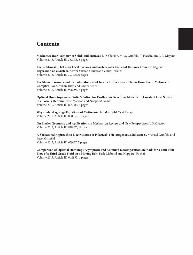

2 Advances in Mathematical Physics
with problems in electricalmagnetic and gravitational fieldsfor the paths of defined space-moving objects
In ldquoThe Steiner Formula and the Polar Moment of Inertiafor the Closed Planar Homothetic Motions in ComplexPlanerdquo the coauthors A Tutar and O Sener express theSteiner area formula and the polar moment of inertia duringone-parameter closed planar homothetic motions in thecomplex plane The Steiner point or Steiner normal conceptsare described according to whether a rotation number isdifferent from zero or equal to zero respectively The movingpole point is given with its components and its relationbetween a Steiner point and a Steiner normal is specifiedThesagittal motion of a winch is considered as an example Thismotion is described by a double hinge consisting of the fixedcontrol panel of the winch and its moving arm The winchis studied here because its arm can extend or retract duringone-parameter closed planar homothetic motions
3 Electrostatics
In ldquoA Variational Approach to Electrostatics of PolarizableHeterogeneous Substancesrdquo the coauthors M Grinfeld andP Grinfeld discuss equilibrium conditions for heterogeneoussubstances subject to electrostatic or magnetostatic effectsThe goal of this paper is to present a logically consistentextension of the Gibbs variational approach [2] to elasticbodies with interfaces in the presence of electromagneticeffects It is demonstrated that the force-like aleph tensorand the energy-like beth tensor for polarizable deformablesubstances are divergence-free Two additional tensors areintroduced the divergence-free energy-like gimel tensorfor rigid dielectrics and the general electrostatic gammatensor which is not necessarily divergence-free The presentapproach is based on a logically consistent extension of theGibbs energy principle that takes into account polarizationeffects
Contrary to many prior attempts explicitly excluded arethe electric field and the electric displacement from the list ofindependent thermodynamic variables Instead polarizationis treated by adding a single term to the traditional free energyfor a thermoelastic systemThe additional term represents thepotential energy accumulated in the electrostatic field overthe entire space The exact nonlinear theory of continuousmedia is invoked with Eulerian coordinates as the indepen-dent spatial variables
While the proposed model is mathematically rigorousthe authors caution against the assumption that it can reliablypredict physical phenomena On the contrary clear modelsoften lead to conclusions at odds with experiment andtherefore should be treated as physical paradoxes that deservethe attention of the scientific community
4 Solid Mechanics
In ldquoOn Finsler Geometry and Applications in MechanicsReview and New Perspectivesrdquo the author J D Claytonbegins with a review of necessary mathematical definitionsand derivations and then reviews prior work involvingapplication of Finsler geometry in continuum mechanics of
solids The use of Finsler geometry (eg [5]) to describecontinuum mechanical behavior of solids was suggestednearly five decades ago by Kroner in 1968 [1] As overlookedin the initial review by the author Finsler geometry wasapplied towards deforming ferromagnetic crystals by Amariin 1962 [3] and has somewhat recently been applied to frac-ture mechanics problems [6] Building on theoretical workof Ikeda [7] Bejancu [8] distinguished among horizontaland vertical distributions of the fiber bundle of a finite-deforming pseudo-Finslerian total space More completetheories incorporating a Lagrangian functional (leading tophysical balance or conservation laws) and couched in termsof Finsler geometry were developed by Stumpf and Saczukfor describing inelasticity mechanisms such as plasticity anddamage [9] including the only known published solutions ofboundary value problems incorporating such sophistication
This contributed paper by J D Clayton also introducesaspects of a new theoretical description of mechanics ofcontinua with microstructure This original theory thoughneither complete nor fully explored combines ideas fromfinite deformation kinematics [10] Finsler geometry [5 8]and phase field theories of materials physics Future work willenable encapsulation of phase field modeling of fracture andpossible electromechanical couplingwithin Finsler geometricframework
5 Thermal-Fluid Mechanics
In ldquoComparison of Optimal Homotopy Asymptotic andAdomian Decomposition Methods for a Thin Film Flow ofa Third Grade Fluid on a Moving Beltrdquo the coauthors FMabood and N Pochai investigate a thin film flow of athird-grade fluid on a moving belt using a powerful andrelatively new approximate analytical technique known asthe Optimal Homotopy Asymptotic Method (OHAM) Dueto model complexities difficulties often arise in obtainingsolutions of governing nonlinear differential equations fornon-Newtonian fluids A second-grade fluid is one of themost acceptable fluids in this class because of its mathemati-cal simplicity in comparison to third-grade and fourth-gradefluids In related literature many authors have effectivelytreated the complicated nonlinear equations governing theflow of a third-grade fluid In this study it is observedthat the OHAM is a powerful approximate analytical toolthat is simple and straightforward and does not requirethe existence of any small or large parameter as does thetraditional perturbationmethodThe variation of the velocityprofile for different parameters is compared with numericalvalues obtained by the Runge-Kutta-Fehlberg fourth-fifth-ordermethod andwith theAdomianDecompositionMethod(ADM) An interesting result of the analysis is that the three-term OHAM solution is more accurate than five-term ADMsolution confirming feasibility of the former method
In ldquoOptimalHomotopyAsymptotic Solution for Exother-mic Reactions Model with Constant Heat Source in a PorousMediumrdquo the coauthors F Mabood and N Pochai consideranalytical and numerical treatments of heat transfer inparticular problems Heat flow patternsprofiles are requiredfor heat transfer simulation in various types of thermal
Advances in Mathematical Physics 3
insulationThe exothermic reactionmodels for porousmediacan often be prescribed in the form of sets of nonlinearordinary differential equations In this research the drivingforce model due to temperature gradients is considered Agoverning equation of the model is restructured into anenergy balance equation that provides the temperature profilein a conduction state with a constant heat source in thesteady state A proposed Optimal Homotopy AsymptoticMethod (OHAM) is used to compute the solutions of theexothermic reactions equations The posited OHAM schemeis convenient to implement has fourth-order accuracy anddemonstrates no obvious problematic instabilities
J D ClaytonM A Grinfeld
T HasebeJ R Mayeur
References
[1] E Kroner ldquoInterrelations between various branches of con-tinuum mechanicsrdquo in Mechanics of Generalized Continua EKroner Ed pp 330ndash340 Springer Berlin Germany 1968
[2] M A Grinfeld Thermodynamic Methods in the Theory ofHeterogeneous Systems Longman Sussex UK 1991
[3] S Amari ldquoA theory of deformations and stresses of ferromag-netic substances by Finsler geometryrdquo in RAAG Memoirs KKondo Ed vol 3 pp 257ndash278 1962
[4] J D Clayton Nonlinear Mechanics of Crystals Springer Dor-drecht The Netherlands 2011
[5] H Rund The Differential Geometry of Finsler Spaces SpringerBerlin Germany 1959
[6] I A Miklashevich ldquoGeometric characteristics of fracture-associated space and crack propagation in a materialrdquo Journalof Applied Mechanics and Technical Physics vol 44 no 2 pp255ndash261 2003
[7] S Ikeda ldquoA physico-geometrical consideration on the theoryof directors in the continuum mechanics of oriented mediardquoTensor New Series vol 27 pp 361ndash368 1973
[8] A Bejancu Finsler Geometry and Applications Ellis HorwoodNew York NY USA 1990
[9] H Stumpf and J Saczuk ldquoA generalized model of oriented con-tinuum with defectsrdquo Zeitschrift fur Angewandte Mathematikund Mechanik vol 80 no 3 pp 147ndash169 2000
[10] J D ClaytonDifferential Geometry and Kinematics of ContinuaWorld Scientific Singapore 2014
Research ArticleThe Relationship between Focal Surfaces and Surfaces ata Constant Distance from the Edge of Regression on a Surface
Semra Yurttancikmaz and Omer Tarakci
Department of Mathematics Faculty of Science Ataturk University 25240 Erzurum Turkey
Correspondence should be addressed to Semra Yurttancikmaz semrakayaatauniedutr
Received 7 July 2014 Accepted 8 September 2014
Academic Editor John D Clayton
Copyright copy 2015 S Yurttancikmaz and O Tarakci This is an open access article distributed under the Creative CommonsAttribution License which permits unrestricted use distribution and reproduction in any medium provided the original work isproperly cited
We investigate the relationship between focal surfaces and surfaces at a constant distance from the edge of regression on a surfaceWe show that focal surfaces F
1and F
2of the surface M can be obtained by means of some special surfaces at a constant distance
from the edge of regression on the surfaceM
1 Introduction
Surfaces at a constant distance from the edge of regression ona surface were firstly defined by Tarakci in 2002 [1] Thesesurfaces were obtained by taking a surface instead of acurve in the study suggested by Hans Vogler in 1963 In thementioned study Hans Vogler asserted notion of curve at aconstant distance from the edge of regression on a curveAlso Tarakci and Hacisalihoglu calculated some propertiesand theorems which known for parallel surfaces for surfacesat a constant distance from the edge of regression on a surface[2] Later various authors became interested in surfaces at aconstant distance from the edge of regression on a surface andinvestigated Euler theorem and Dupin indicatrix conjugatetangent vectors and asymptotic directions for this surface [3]and examined surfaces at a constant distance from the edgeof regression on a surface in 1198643
1Minkowski space [4]
Another issue that we will use in this paper is the focalsurface Focal surfaces are known in the field of line con-gruence Line congruence has been introduced in the field ofvisualization by Hagen et al in 1991 [5] They can be used tovisualize the pressure and heat distribution on an airplanetemperature rainfall ozone over the earthrsquos surface andso forth Focal surfaces are also used as a surface interrogationtool to analyse the ldquoqualityrdquo of the surface before furtherprocessing of the surface for example in a NC-milling oper-ation [6] Generalized focal surfaces are related to hedgehog
diagrams Instead of drawing surface normals proportionalto a surface value only the point on the surface normalproportional to the function is drawing The loci of all thesepoints are the generalized focal surface This method wasintroduced byHagen andHahmann [6 7] and is based on theconcept of focal surface which is known from line geometryThe focal surfaces are the loci of all focal points of specialcongruence the normal congruence In later years focalsurfaces have been studied by various authors in differentfields
In this paper we have discovered a new method to con-stitute focal surfaces by means of surfaces at a constantdistance from the edge of regression on a surface Focalsurfaces 119865
1and 119865
2of the surface119872 in 1198643 are associated with
surfaces at a constant distance from the edge of regressionon 119872 that formed along directions of 119885
119875lying in planes
119878119901120601119906 119873 and 119878119901120601V 119873 respectively
2 Surfaces at a Constant Distance fromthe Edge of Regression on a Surface
Definition 1 Let119872 and119872119891 be two surfaces in 1198643 Euclideanspace and let 119873
119875be a unit normal vector and let 119879
119875119872 be
tangent space at point 119875 of surface 119872 and let 119883119875 119884119875 be
orthonormal bases of 119879119875119872 Take a unit vector 119885
119875= 1198891119883119875+
Hindawi Publishing CorporationAdvances in Mathematical PhysicsVolume 2015 Article ID 397126 6 pageshttpdxdoiorg1011552015397126
2 Advances in Mathematical Physics
1198892119884119875+1198893119873119875 where 119889
1 1198892 1198893isin R are constant and 1198892
1+1198892
2+
1198892
3= 1 If there is a function 119891 defined by
119891 119872 997888rarr 119872119891 119891 (119875) = 119875 + 119903119885
119875 (1)
where 119903 isin R then the surface 119872119891 is called the surface at aconstant distance from the edge of regression on the surface119872
Here if 1198891= 1198892= 0 then119885
119875= 119873119875and so119872 and119872119891 are
parallel surfaces Now we represent parametrization of sur-faces at a constant distance from the edge of regression on119872Let (120601 119880) be a parametrization of119872 so we can write that
120601 119880 sub 1198642997888rarr 119872
(119906 V) 120601 (119906 V) (2)
In case 120601119906 120601V is a basis of 119879
119875119872 then we can write that
119885119875= 1198891120601119906+1198892120601V+1198893119873119875 where120601119906 120601V are respectively partial
derivatives of 120601 according to 119906 and V Since 119872119891 = 119891(119875)
119891(119875) = 119875 + 119903119885119875 a parametric representation of119872119891 is
120595 (119906 V) = 120601 (119906 V) + 119903119885 (119906 V) (3)
Thus it is obtained that
119872119891= 120595 (119906 V) 120595 (119906 V)
= 120601 (119906 V)
+ 119903 (1198891120601119906(119906 V)
+ 1198892120601V (119906 V)
+ 1198893119873(119906 V))
(4)
and if we get 1199031198891= 1205821 1199031198892= 1205822 1199031198893= 1205823 then we have
119872119891= 120595 (119906 V) 120595 (119906 V)
= 120601 (119906 V) + 1205821120601119906(119906 V)
+ 1205822120601V (119906 V) + 1205823119873(119906 V)
1205822
1+ 1205822
2+ 1205822
3= 1199032
(5)
Calculation of 120595119906and 120595V gives us that
120595119906= 120601119906+ 1205821120601119906119906+ 1205822120601V119906 + 1205823119873119906
120595V = 120601V + 1205821120601119906V + 1205822120601VV + 1205823119873V(6)
Here 120601119906119906 120601V119906 120601119906V 120601VV 119873119906 119873V are calculated as in [1] We
choose curvature lines instead of parameter curves of119872 andlet 119906 and V be arc length of these curvature lines Thus thefollowing equations are obtained
120601119906119906= minus 120581
1119873
120601VV = minus 1205812119873
120601119906V = 120601V119906 = 0
119873119906= 1205811120601119906
119873V = 1205812120601V
(7)
From (6) and (7) we find
120595119906= (1 + 120582
31205811) 120601119906minus 12058211205811119873
120595V = (1 + 12058231205812) 120601V minus 12058221205812119873
(8)
and 120595119906 120595V is a basis of 120594(119872119891) If we denote by 119873119891 unit
normal vector of119872119891 then119873119891 is
119873119891=
[120595119906 120595V]
1003817100381710038171003817[120595119906 120595V]1003817100381710038171003817
= (12058211205811(1 + 120582
31205812) 120601119906+ 12058221205812(1 + 120582
31205811) 120601V
+ (1 + 12058231205811) (1 + 120582
31205812)119873)
times (1205822
11205812
1(1 + 120582
31205812)2
+ 1205822
21205812
2(1 + 120582
31205811)2
+ (1 + 12058231205811)2
(1 + 12058231205812)2
)minus12
(9)
where 1205811 1205812are principal curvatures of the surface119872 If
119860 = (1205822
11205812
1(1 + 120582
31205812)2
+ 1205822
21205812
2(1 + 120582
31205811)2
+(1 + 12058231205811)2
(1 + 12058231205812)2
)12
(10)
we can write
119873119891=12058211205811(1 + 120582
31205812)
119860120601119906+12058221205812(1 + 120582
31205811)
119860120601V
+(1 + 120582
31205811) (1 + 120582
31205812)
119860119873
(11)
Here in case of 1205811= 1205812and 120582
3= minus1120581
1= minus1120581
2since120595
119906and
120595V are not linearly independent119872119891 is not a regular surface
We will not consider this case [1]
3 Focal Surfaces
The differential geometry of smooth three-dimensional sur-faces can be interpreted from one of two perspectives interms of oriented frames located on the surface or in termsof a pair of associated focal surfaces These focal surfacesare swept by the loci of the principal curvatures radiiConsidering fundamental facts from differential geometry itis obvious that the centers of curvature of the normal sectioncurves at a particular point on the surface fill out a certainsegment of the normal vector at this pointThe extremities ofthese segments are the centers of curvature of two principaldirections These two points are called the focal points ofthis particular normal [8] This terminology is justified bythe fact that a line congruence can be considered as theset of lines touching two surfaces the focal surfaces of theline congruence The points of contact between a line of thecongruence and the two focal surfaces are the focal pointsof this line It turns out that the focal points of a normalcongruence are the centers of curvature of the two principaldirections [9 10]
Advances in Mathematical Physics 3
We represent surfaces parametrically as vector-valuedfunctions 120601(119906 V) Given a set of unit vectors 119885(119906 V) a linecongruence is defined
119862 (119906 V) = 120601 (119906 V) + 119863 (119906 V) 119885 (119906 V) (12)
where 119863(119906 V) is called the signed distance between 120601(119906 V)and 119885(119906 V) [8] Let 119873(119906 V) be unit normal vector of thesurface If 119885(119906 V) = 119873(119906 V) then 119862 = 119862
119873is a normal
congruence A focal surface is a special normal congruenceThe parametric representation of the focal surfaces of 119862
119873is
given by
119865119894(119906 V) = 120601 (119906 V) minus
1
120581119894(119906 V)
119873 (119906 V) 119894 = 1 2 (13)
where 1205811 1205812are the principal curvatures Except for parabolic
points and planar points where one or both principal curva-tures are zero each point on the base surface is associatedwith two focal points Thus generally a smooth base surfacehas two focal surface sheets 119865
1(119906 V) and 119865
2(119906 V) [11]
The generalization of this classical concept leads to thegeneralized focal surfaces
119865 (119906 V) = 120601 (119906 V) + 119886119891 (1205811 1205812)119873 (119906 V) with 119886 isin R (14)
where the scalar function 119891 depends on the principal curva-tures 120581
1= 1205811(119906 V) and 120581
2= 1205812(119906 V) of the surface119872The real
number 119886 is used as a scale factor If the curvatures are verysmall you need a very large number 119886 to distinguish the twosurfaces 120601(119906 V) and 119865(119906 V) on the screen Variation of thisfactor can also improve the visibility of several properties ofthe focal surface for example one can get intersectionsclearer [6]
4 The Relationship between Focal Surfacesand Surfaces at a Constant Distance fromthe Edge of Regression on a Surface
Theorem 2 Let surface 119872 be given by parametrical 120601(119906 V)One considers all surfaces at a constant distance from the edgeof regression on 119872 that formed along directions of 119885
119875lying
in plane 119878119901120601119906 119873 Normals of these surfaces at points 119891(119875)
corresponding to point 119875 isin 119872 generate a spatial family of lineof which top is center of first principal curvature 119862
1= 119875minus
(11205811(119875))119873
119875at 119875
Proof Surfaces at a constant distance from the edge of reg-ression on 119872 that formed along directions of 119885
119875lying in
plane 119878119901120601119906 119873 are defined by
119891119894 119872 997888rarr 119872
119891119894 119894 = 1 2
119891119894(119875) = 119875 + 120582
1119894120601119906(119875) + 120582
3119894119873119875
(15)
These surfaces and their unit normal vectors are respectivelydenoted by119872119891119894 and 119873119891119894 We will demonstrate that intersec-tion point of lines which pass from the point 119891
119894(119875) and are in
direction119873119891119894119891119894(119875)
is 1198621= 119875 minus (1120581
1(119875))119873
119875
The normal vector of the surface119872119891119894 at the point 119891119894(119875) is
119873119891119894 = 120582
11198941205811(119875) 120601119906(119875) + (1 + 120582
31198941205811(119875))119873
119875 (16)
Here it is clear that 119873119891119894 is in plane 119878119901120601119906 119873 Suppose that
line passing from the point119891119894(119875) and being in direction119873119891119894
119891119894(119875)
is 119889119894and a representative point of 119889
119894is119876 = (119909 119910) = 119909120601
119906(119875) +
119910119873119875 then the equation of 119889
119894is
119889119894sdot sdot sdot
997888997888rarr119875119876 =
997888997888997888997888997888rarr119875119891119894(119875) + 120583
1119873119891119894
119891119894(119875) (17)
Besides suppose that line passing from the point 119891119895(119875) and
being in direction119873119891119895119891119895(119875)
is 119889119895and a representative point of 119889
119895
is 119877 = (119909 119910) then equation of 119889119895is
119889119895sdot sdot sdot
997888rarr119875119877 =
997888997888997888997888997888rarr119875119891119895(119875) + 120583
2119873119891119895
119891119895(119875) 119895 = 1 2 (18)
We find intersection point of these lines Since it is studiedin plane of vectors 120601
119906(119875)119873
119875 the point 119875 can be taken as
beginning point If we arrange the lines 119889119894and 119889
119895 then we
find
119889119894sdot sdot sdot (119909 119910) = (120582
1119894 1205823119894) + 1205831(12058211198941205811 1 + 120582
31198941205811)
119889119894sdot sdot sdot 119910 =
1 + 12058231198941205811
12058211198941205811
119909 minus1
1205811
119889119895sdot sdot sdot (119909 119910) = (120582
1119895 1205823119895) + 1205832(12058211198951205811 1 + 120582
31198951205811)
119889119895sdot sdot sdot 119910 =
1 + 12058231198951205811
12058211198951205811
119909 minus1
1205811
(19)
From here it is clear that intersection point of 119889119894and 119889
119895is
(119909 119910) = (0 minus11205811) So intersection point of the lines119889
119894and119889119895
is the point1198621= 119875minus(1120581
1(119875))119873
119875in plane 119878119901120601
119906(119875)119873
119875
Corollary 3 Directions of normals of all surfaces at a constantdistance from the edge of regression on 119872 that formed alongdirections of 119885
119875lying in plane 119878119901120601
119906 119873 intersect at a single
point This point 1198621= 119875 minus (1120581
1(119875))119873
119875which is referred in
Theorem 2 is on the focal surface 1198651
We know that
1198651(119875) = 119875 minus
1
1205811
119873119875 (20)
from definition of focal surfaces Moreover we can see easilythe following equations from Figure 1
1198651(119875) = 119891
119894(119875) minus 120583
119894119873119891119894
119891119894(119875)(21)
or
1198651(119875) = 119891
119895(119875) minus 120583
119895119873119891119895
119891119895(119875) (22)
These equations show us that the focal surface 1198651of the sur-
face119872 can be stated by surfaces at a constant distance from
4 Advances in Mathematical Physics
the edge of regression on119872 that formed along directions of119885119875lying in plane 119878119901120601
119906 119873 If 120583
119894= 1120581
119891119894
1or 120583119895= 1120581
119891119895
1 then
the focal surfaces 1198651of surfaces119872 119872
119891119894 and119872119891119895 will be thesame This case has been expressed in following theorem
Theorem 4 Focal surfaces 1198651of the surface119872 and surfaces at
a constant distance from the edge of regression on119872 that for-med along directions of 119885
119875lying in plane 119878119901120601
119906 119873 are the
same if and only if first principal curvature 1205811of the surface
119872 is constant
Proof Suppose that focal surfaces 1198651of surfaces119872 and119872119891
formed along directions of 119885119875
lying in plane 119878119901120601119906 119873
intersect then 120583119894mentioned in (21) must be
120583119894=
1
120581119891119894
1
(23)
First principal curvature 1205811198911of119872119891 formed along directions of
119885119875lying in plane 119878119901120601
119906 119873 that is for 120582
2= 0 is calculated
by Tarakci as [1]
120581119891
1=
1
radic1205822
11205812
1+ (1 + 120582
31205811)2
(1205821(1205971205811120597119906)
1205822
11205812
1+ (1 + 120582
31205811)2+ 1205811)
(24)
Besides from Figure 1 since 120583119894= |
997888997888997888997888997888997888rarr1198621119891119894(119875)| is distance bet-
ween points of 1198621= (0 minus1120581
1) and 119891
119894(119875) = (120582
1 1205823) lying in
plane 119878119901120601119906 119873 we can write
120583119894=
1003816100381610038161003816100381610038161003816
997888997888997888997888997888997888rarr1198621119891119894(119875)
1003816100381610038161003816100381610038161003816= radic1205822
1+ (1205823+1
1205811
)
2
(25)
If we substitute (24) and (25) in (23) and make necessaryarrangements we obtain
1205971205811
120597119906= 0 (26)
Thus we have 1205811= const The converse statement is trivial
Hence our theorem is proved
Theorem 5 Let surface 119872 be given by parametrical 120601(119906 V)We consider all surfaces at a constant distance from the edgeof regression on119872 that formed along directions of 119885
119875lying in
plane 119878119901120601V 119873 Normals of these surfaces at points 119891(119875)corresponding to point 119875 isin 119872 generate a spatial family of lineof which top is center of second principal curvature 119862
2= 119875minus
(11205812(119875))119873
119875at 119875
Proof Surfaces at a constant distance from the edge of regre-ssion on119872 that formed along directions of 119885
119875lying in plane
119878119901120601V 119873 are defined by
119891119894 119872 997888rarr 119872
119891119894 119894 = 1 2
119891119894(119875) = 119875 + 120582
2119894120601V (119875) + 1205823119894119873119875
(27)
M
F1
dj
di
C1 = F1(P)
P 120601u
NPZP119894
ZP119895
fi(P)
fj(P)
Nf119894
Nf119895Mf119894
Mf119895
1
1205811
Figure 1 Directions of normals of all surfaces at a constant distancefrom the edge of regression on119872 that formed along directions of119885
119875
lying in plane 119878119901120601119906 119873 and their intersection point (focal point)
These surfaces and their unit normal vectors are respectivelydenoted by119872119891119894 and 119873119891119894 We will demonstrate that intersec-tion point of lines which pass from the point 119891
119894(119875) and are in
direction119873119891119894119891119894(119875)
is 1198622= 119875 minus (1120581
2(119875))119873
119875
The normal vector of the surface119872119891119894 at the point 119891119894(119875) is
119873119891119894 = 120582
21198941205812(119875) 120601V (119875) + (1 + 12058231198941205812 (119875))119873119875 (28)
Here it is clear that 119873119891119894 is in plane 119878119901120601V 119873 Suppose thatline passing from the point119891
119894(119875) and being in direction119873119891119894
119891119894(119875)
is 119889119894and a representative point of 119889
119894is 119876 = (119909 119910) = 119909120601V(119875) +
119910119873119875 then equation of 119889
119894is
119889119894sdot sdot sdot
997888997888rarr119875119876 =
997888997888997888997888997888rarr119875119891119894(119875) + 120583
1119873119891119894
119891119894(119875) (29)
Besides suppose that line passing from the point 119891119895(119875) of the
surface119872119891119895 and being in direction119873119891119895119891119895(119875)
is119889119895and a represen-
tative point of 119889119895is 119877 = (119909 119910) then equation of 119889
119895is
119889119895sdot sdot sdot
997888rarr119875119877 =
997888997888997888997888997888rarr119875119891119895(119875) + 120583
2119873119891119895
119891119895(119875) 119895 = 1 2 (30)
We find intersection point of these two lines Since it is stud-ied in plane of vectors 120601V(119875)119873119875 the point 119875 can be taken
Advances in Mathematical Physics 5
as beginning point If we arrange the lines 119889119894and 119889
119895 then we
find
119889119894sdot sdot sdot (119909 119910) = (120582
2119894 1205823119894) + 1205831(12058221198941205811 1 + 120582
31198941205812)
119889119894sdot sdot sdot 119910 =
1 + 12058231198941205812
12058221198941205812
119909 minus1
1205812
119889119895sdot sdot sdot (119909 119910) = (120582
2119895 1205823119895) + 1205832(12058221198951205812 1 + 120582
31198951205812)
119889119895sdot sdot sdot 119910 =
1 + 12058231198951205812
12058221198951205812
119909 minus1
1205812
(31)
From here it is clear that intersection point of 119889119894and 119889
119895is
(119909 119910) = (0 minus11205812) So intersection point of the lines 119889
119894and
119889119895is the point 119862
2= 119875 minus (1120581
2(119875))119873
119875in plane 119878119901120601V(119875)119873119875
Corollary 6 Thepoint1198622= 119875minus(1120581
2(119875))119873
119875which is referred
in Theorem 5 is on the focal surface 1198652
Similar to Figure 1 we can write equations
1198652(119875) = 119891
119894(119875) minus 120583
119894119873119891119894
119891119894(119875)(32)
or
1198652(119875) = 119891
119895(119875) minus 120583
119895119873119891119895
119891119895(119875) (33)
These equations show us that the focal surface 1198652of the sur-
face119872 can be stated by surfaces at a constant distance fromthe edge of regression on119872 that formed along directions of119885119875lying in plane 119878119901120601V 119873 If 120583119894 = 1120581
119891119894
2or 120583119895= 1120581
119891119895
2 then
the focal surfaces 1198652of surfaces119872 119872
119891119894 and119872119891119895 will be thesame This case has been expressed in following theorem
Theorem 7 Focal surfaces 1198652of the surface119872 and surfaces at
a constant distance from the edge of regression on119872 that for-med along directions of 119885
119875lying in plane 119878119901120601V 119873 are the
same if and only if second principal curvature 1205812of the surface
119872 is constant
Proof Suppose that focal surfaces 1198652of surfaces119872 and119872119891
formed along directions of 119885119875
lying in plane 119878119901120601V 119873
intersect then 120583119894mentioned in (32) must be
120583119894=
1
120581119891119894
2
(34)
Second principal curvature 1205811198912of119872119891 formed along directions
of119885119875lying in plane 119878119901120601V 119873 that is for 1205821 = 0 is calculated
by Tarakci as [1]
120581119891
2=
1
radic1205822
21205812
2+ (1 + 120582
31205812)2
(1205822(1205971205812120597V)
1205822
21205812
2+ (1 + 120582
31205812)2+ 1205812)
(35)
Besides similar to Figure 1 since120583119894= |997888997888997888997888997888997888rarr1198622119891119894(119875)| is the distance
between points of 1198622= (0 minus1120581
2) and 119891
119894(119875) = (120582
2 1205823) lying
in plane 119878119901120601V 119873 we can write
120583119894=
1003816100381610038161003816100381610038161003816
997888997888997888997888997888997888rarr1198622119891119894(119875)
1003816100381610038161003816100381610038161003816= radic1205822
2+ (1205823+1
1205812
)
2
(36)
If we substitute (35) and (36) in (34) and make necessaryarrangements we obtain
1205971205812
120597V= 0 (37)
Thus we have 1205812= const The converse statement is trivial
Hence our theorem is proved
Points on the surface119872 can have the same curvature in alldirections These points correspond to the umbilics aroundwhich local surface is sphere-like Since normal rays of umbi-lic points pass through a single point the focal mesh formedby vertices around an umbilic point can shrink into a point[11]
Conflict of Interests
The authors declare that there is no conflict of interestsregarding the publication of this paper
References
[1] O Tarakci Surfaces at a constant distance from the edge of reg-ression on a surface [PhD thesis] Ankara University Institute ofScience Ankara Turkey 2002
[2] O Tarakci and H H Hacisalihoglu ldquoSurfaces at a constantdistance from the edge of regression on a surfacerdquo AppliedMathematics and Computation vol 155 no 1 pp 81ndash93 2004
[3] N Aktan A Gorgulu E Ozusaglam and C Ekici ldquoConjugatetangent vectors and asymptotic directions for surfaces at aconstant distance from edge of regression on a surfacerdquo Inter-national Journal of Pure and Applied Mathematics vol 33 no 1pp 127ndash133 2006
[4] D Saglam and O Kalkan ldquoSurfaces at a constant distance fromthe edge of regression on a surface in 119864
3
1rdquo Differential Geo-
metrymdashDynamical Systems vol 12 pp 187ndash200 2010[5] H Hagen H Pottmann and A Divivier ldquoVisualization func-
tions on a surfacerdquo Journal of Visualization and Animation vol2 pp 52ndash58 1991
[6] H Hagen and S Hahmann ldquoGeneralized focal surfaces a newmethod for surface interrogationrdquo in Proceedings of the IEEEConference on Visualization (Visualization rsquo92) pp 70ndash76 Bos-ton Mass USA October 1992
[7] H Hagen and S Hahmann ldquoVisualization of curvature behav-iour of free-form curves and surfacesrdquo Computer-Aided Designvol 27 no 7 pp 545ndash552 1995
[8] H Hagen S Hahmann T Schreiber Y Nakajima B Worden-weber and P Hollemann-Grundstedt ldquoSurface interrogationalgorithmsrdquo IEEE Computer Graphics and Applications vol 12no 5 pp 53ndash60 1992
6 Advances in Mathematical Physics
[9] J Hoschek Linien-Geometrie BI Wissensehaffs Zurich Swit-zerland 1971
[10] K StrubeckerDifferentialgeometrie III DeGruyter Berlin Ger-many 1959
[11] J Yu X Yin X Gu L McMillan and S Gortler ldquoFocal Surfacesof discrete geometryrdquo in Eurographics Symposium on GeometryProcessing 2007
Research ArticleThe Steiner Formula and the Polar Moment of Inertia for theClosed Planar Homothetic Motions in Complex Plane
Ayhan Tutar and Onder Sener
Department of Mathematics Ondokuz Mayis University Kurupelit 55139 Samsun Turkey
Correspondence should be addressed to Ayhan Tutar atutaromuedutr
Received 29 December 2014 Accepted 23 February 2015
Academic Editor John D Clayton
Copyright copy 2015 A Tutar and O Sener This is an open access article distributed under the Creative Commons AttributionLicense which permits unrestricted use distribution and reproduction in any medium provided the original work is properlycited
The Steiner area formula and the polar moment of inertia were expressed during one-parameter closed planar homothetic motionsin complex planeThe Steiner point or Steiner normal concepts were described according to whether rotation number was differentfrom zero or equal to zero respectivelyThemoving pole point was given with its components and its relation between Steiner pointor Steiner normalwas specifiedThe sagittalmotion of awinchwas considered as an exampleThismotionwas described by a doublehinge consisting of the fixed control panel of winch and the moving arm of winch The results obtained in the second section ofthis study were applied for this motion
1 Introduction
For a geometrical object rolling on a line and making acomplete turn some properties of the area of a path of a pointwere given by [1] The Steiner area formula and the Holditchtheorem during one-parameter closed planar homotheticmotions were expressed by [2] We calculated the expressionof the Steiner formula relative to the moving coordinate sys-tem under one-parameter closed planar homothetic motionsin complex plane If the points of the moving plane whichenclose the same area lie on a circle then the centre of thiscircle is called the Steiner point (ℎ = 1) [3 4] If thesepoints lie on a line we use Steiner normal instead of SteinerpointThen we obtained the moving pole point for the closedplanar homothetic motions We dealt with the polar momentof inertia of a path generated by a closed planar homotheticmotion Furthermore we expressed the relation between thearea enclosed by a path and the polar moment of inertia Asan example the sagittal motion of a winch which is describedby a double hinge being fixed and moving was consideredThe Steiner area formula the moving pole point and thepolar moment of inertia were calculated for this motionMoreover the relation between the Steiner formula and thepolar moment of inertia was expressed
2 Closed Homothetic Motions inComplex Plane
We consider one-parameter closed planar homotheticmotion between two reference systems the fixed 119864
1015840 andthe moving 119864 with their origins (119874 119874
1015840) and orientations in
complex planeThen we take into account motion relative tothe fixed coordinate system (direct motion)
By taking displacement vectors 1198741198741015840= 119880 and 119874
1015840119874 = 119880
1015840
and the total angle of rotation 120572(119905) the motion defined by thetransformation
1198831015840(119905) = ℎ (119905)119883119890
119894120572(119905)+ 1198801015840(119905) (1)
is called one-parameter closed planar homotheticmotion anddenoted by 1198641198641015840 where ℎ is a homothetic scale of the motion1198641198641015840 and119883 and1198831015840 are the position vectors with respect to the
moving and fixed rectangular coordinate systems of a point119883 isin 119864 respectively The homothetic scale ℎ and the vectors1198831015840 and 119880119880
1015840 are continuously differentiable functions of areal parameter 119905
In (1) 1198831015840(119905) is the trajectory with respect to the fixedsystem of a point 119883 belonging to the moving system If wereplace 1198801015840 = minus119880119890
119894120572(119905) in (1) the motion can be written as
1198831015840(119905) = (ℎ (119905)119883 minus 119880 (119905)) 119890
119894120572(119905) (2)
Hindawi Publishing CorporationAdvances in Mathematical PhysicsVolume 2015 Article ID 978294 5 pageshttpdxdoiorg1011552015978294
2 Advances in Mathematical Physics
The coordinates of the above equation are
1198831015840(119905) = 119909
1015840
1(119905) + 119894119909
1015840
2(119905) 119880
1015840(119905) = 119906
1015840
1(119905) + 119894119906
1015840
2(119905)
119883 = 1199091+ 1198941199092 119880 (119905) = 119906
1(119905) + 119894119906
2(119905)
(3)
Using these coordinates we can write
1199091015840
1(119905) + 119894119909
1015840
2(119905) = [(ℎ (119905) 119909
1minus 1199061) + 119894 (ℎ (119905) 119909
2minus 1199062)]
sdot (cos120572 (119905) + 119894 sin120572 (119905))
(4)
From (4) the components of1198831015840(119905)may be given as
1199091015840
1(119905) = cos (120572 (119905)) (ℎ (119905) 119909
1minus 1199061) minus sin (120572 (119905)) (ℎ (119905) 119909
2minus 1199062)
1199091015840
2(119905) = sin (120572 (119905)) (ℎ (119905) 119909
1minus 1199061) + cos (120572 (119905)) (ℎ (119905) 119909
2minus 1199062)
(5)
Using the coordinates of (2) as
1198831015840(119905) = (
1199091015840
1(119905)
1199091015840
2(119905)
) 1198801015840(119905) = (
1199061015840
1(119905)
1199061015840
2(119905)
)
119883 = (
1199091
1199092
) 119880 (119905) = (
1199061(119905)
1199062(119905)
)
(6)
and rotation matrix
119877 (119905) = (
cos (120572 (119905)) minus sin (120572 (119905))
sin (120572 (119905)) cos (120572 (119905))) (7)
we can obtain
1198831015840(119905) = 119877 (119905) (ℎ (119905)119883 minus 119880 (119905)) (8)
If we differentiate (5) we have
1198891199091015840
1= minus sin120572 (ℎ119909
1minus 1199061) 119889120572 + cos120572 (119889ℎ119909
1minus 1198891199061)
minus cos120572 (ℎ1199092minus 1199062) 119889120572 minus sin120572 (119889ℎ119909
2minus 1198891199062)
1198891199091015840
2= cos120572 (ℎ119909
1minus 1199061) 119889120572 + sin120572 (119889ℎ119909
1minus 1198891199061)
minus sin120572 (ℎ1199092minus 1199062) 119889120572 + cos120572 (119889ℎ119909
2minus 1198891199062)
(9)
21 The Steiner Formula for the Homothetic Motions Theformula for the area 119865 of a closed planar curve of the point1198831015840 is given by
119865 =1
2∮(1199091015840
11198891199091015840
2minus 1199091015840
21198891199091015840
1) (10)
If (5) and (9) are placed in (10) we have
2119865 = (1199092
1+ 1199092
2)∮ℎ2119889120572 + 119909
1∮(minus2ℎ119906
1119889120572 minus ℎ119889119906
2+ 1199062119889ℎ)
+ 1199092∮(minus2ℎ119906
2119889120572 + ℎ119889119906
1minus 1199061119889ℎ)
+ ∮(1199062
1+ 1199062
2) 119889120572 + 119906
11198891199062minus 11990621198891199061
(11)
The following expressions are used in (11)
∮(minus2ℎ1199061119889120572 minus ℎ119889119906
2+ 1199062119889ℎ) = 119886
lowast
∮ (minus2ℎ1199062119889120572 + ℎ119889119906
1minus 1199061119889ℎ) = 119887
lowast
∮ (1199062
1+ 1199062
2) 119889120572 + 119906
11198891199062minus 11990621198891199061 = 119888
(12)
The scalar term 119888 which is related to the trajectory of theorigin of themoving systemmay be given as follows by taking119865119900= 119865 (119909
1= 0 119909
2= 0)
2119865119900= 119888 (13)
The coefficient119898
119898 = ∮ℎ2119889120572 = ℎ
2(1199050)∮119889120572 = ℎ
2(1199050) 2120587] (14)
with the rotation number ] determines whether the lines with119865 = const describe circles or straight lines If ] = 0 then wehave circles If ] = 0 the circles reduce to straight lines If (12)(13) and (14) are substituted in (11) then
2 (119865 minus 119865119900) = (119909
2
1+ 1199092
2)119898 + 119886
lowast1199091+ 119887lowast1199092
(15)
can be obtained
211 A Different Parametrization for the Integral CoefficientsEquation (8) by differentiation with respect to 119905 yields
1198891198831015840= 119889119877 (ℎ119883 minus 119880) + 119877 (119889ℎ119883 minus 119889119880) (16)
If119883 = 119875 = (11990111199012) (the pole point) is taken
0 = 1198891198831015840= 119889119877 (ℎ119875 minus 119880) + 119877 (119889ℎ119875 minus 119889119880) (17)
can be written Then if 119880 = (11990611199062) is solved from (17)
1199061= ℎ1199011+ 1199012
119889ℎ
119889120572minus1198891199062
119889120572
1199062= ℎ1199012minus 1199011
119889ℎ
119889120572+1198891199061
119889120572
(18)
are foundIf (18) is placed in (12)
119886lowast= ∮(minus2ℎ
21199011119889120572) + ∮ (minus2ℎ119889ℎ119901
2+ ℎ119889119906
2+ 1199062119889ℎ)
119887lowast= ∮(minus2ℎ
21199012119889120572) + ∮ (2ℎ119889ℎ119901
1minus ℎ119889119906
1minus 1199061119889ℎ)
(19)
can be rewritten Also (19) can be expressed separately as
119886 = ∮ (minus2ℎ21199011119889120572) 119887 = ∮ (minus2ℎ
21199012119889120572) (20)
1205831= ∮ (minus2ℎ119889ℎ119901
2+ ℎ119889119906
2+ 1199062119889ℎ)
1205832= ∮ (2ℎ119889ℎ119901
1minus ℎ119889119906
1minus 1199061119889ℎ)
120583 = (
1205831
1205832
)
(21)
Advances in Mathematical Physics 3
Using (20) and (21) the area formula
2 (119865 minus 119865119900) = (119909
2
1+ 1199092
2)119898 + 119886119909
1+ 1198871199092+ 12058311199091+ 12058321199092
(22)
is found
22 Steiner Point or Steiner Normal for the HomotheticMotions By taking 119898 = 0 the Steiner point 119878 = (119904
1 1199042) for
the closed planar homothetic motion can be written
119904119895=
∮ℎ2119901119895119889120572
∮ℎ2119889120572
119895 = 1 2 (23)
Then
∮ℎ21199011119889120572 = 119904
1119898 ∮ℎ
21199012119889120572 = 119904
2119898 (24)
is found If (24) is placed in (20) and by considering (22)
2 (119865 minus 119865119900) = 119898 (119909
2
1+ 1199092
2minus 211990411199091minus 211990421199092) + 12058311199091+ 12058321199092
(25)
is obtained Equation (25) is called the Steiner area formulafor the closed planar homothetic motion
By dividing this by119898 and by completing the squares oneobtains the equation of a circle
(1199091minus (1199041minus
1205831
2119898))
2
+ (1199092minus (1199042minus
1205832
2119898))
2
minus (1199041minus
1205831
2119898)
2
minus (1199042minus
1205832
2119898)
2
=2 (119865 minus 119865
0)
119898
(26)
All the fixed points of the moving plane which pass aroundequal orbit areas under themotion119864119864
1015840 lie on the same circlewith the center
119872 = (1199041minus
1205831
2119898 1199042minus
1205832
2119898) (27)
in the moving planeIn the case of ℎ(119905) = 1 since 120583
1= 1205832= 0 the point 119872
and the Steiner point 119878 coincide [3] Also by taking 119898 = 0 ifit is replaced in (22) then we have
(119886 + 1205831) 1199091+ (119887 + 120583
2) 1199092minus 2 (119865 minus 119865
0) = 0 (28)
Equation (28) is a straight line If no complete loop occursthen 120578 = 0 and the circles are reduced to straight linesin other words to a circle whose center lies at infinity Thenormal to the lines of equal areas in (28) is given by
119899 = (
119886 + 1205831
119887 + 1205832
) (29)
which is called the Steiner normal [5]
23TheMoving Pole Point for the Homothetic Motions Using(18) if 119875 = (
11990111199012) is solved then the pole point 119875 of the motion
1199011=
119889ℎ (1198891199061minus 1199062119889120572) + ℎ119889120572 (119889119906
2+ 1199061119889120572)
(119889ℎ)2+ ℎ2 (119889120572)
2
1199012=
119889ℎ (1198891199062+ 1199061119889120572) minus ℎ119889120572 (119889119906
1minus 1199062119889120572)
(119889ℎ)2+ ℎ2 (119889120572)
2
(30)
is obtainedFor119898 = 0 using (14) and (23) we arrive at the relation in
(24) between the Steiner point and the pole pointFor 119898 = 0 using (20) and (29) we arrive at the relation
between the Steiner normal and the pole point as follows
(
119886
119887) = (
minus2∮ℎ21199011119889120572
minus2∮ℎ21199012119889120572
) = 119899 minus 120583 (31)
24 The Polar Moments of Inertia for the Homothetic MotionsThe polar moments of inertia ldquo119879rdquo symbolize a path for closedhomothetic motions We find a formula by using 119879119898 and 119899
in this section and we arrive at the relation between the polarmoments of inertia ldquo119879rdquo and the formula of area ldquo119865rdquo (see (37))A relation between the Steiner formula and the polarmomentof inertia around the pole for a moment was given by [6]Muller [3] also demonstrated a relation to the polar momentof inertia around the origin while Tolke [7] inspected thesame relation for closed functions and Kuruoglu et al [8]generalized Mullerrsquos results for homothetic motion
If we use 120572 as a parameter we need to calculate
119879 = ∮(1199091015840
1
2
+ 1199091015840
2
2
) 119889120572 (32)
along the path of119883 Then using (5)
119879 = (1199092
1+ 1199092
2)119898 + 119909
1∮(minus2ℎ119906
1119889120572)
+ 1199092∮(minus2ℎ119906
2119889120572) + ∮(119906
2
1+ 1199062
2) 119889120572
(33)
is obtainedWe need to calculate the polar moments of inertia of the
origin of the moving system therefore 119879119900= 119879 (119909
1= 0 119909
2=
0) one obtains
119879119900= ∮(119906
2
1+ 1199062
2) 119889120572 (34)
If (34) is placed in (33)
119879 minus 119879119900= (1199092
1+ 1199092
2)119898 + 119909
1∮(minus2ℎ119906
1119889120572) + 119909
2∮(minus2ℎ119906
2119889120572)
(35)
can be written Also if (18) is placed in (35)
119879 minus 119879119900= (1199092
1+ 1199092
2)119898 + 119909
1∮(minus2ℎ
21199011119889120572 minus 2ℎ119889ℎ119901
2+ 2ℎ119889119906
2)
+ 1199092∮(minus2ℎ
21199012119889120572 + 2ℎ119889ℎ119901
1minus 2ℎ119889119906
1)
(36)
4 Advances in Mathematical Physics
x1
x2
x9984001
x9984002
L
k
120001
Figure 1 The arms of winch as a double hinge
is obtained and by considering (22) and (36) together wearrive at the relation between the polar moments of inertiaand the formula for the area below
119879 minus 119879119900= 2 (119865 minus 119865
119900) + 1199091∮(ℎ119889119906
2minus 1199062119889ℎ)
+ 1199092∮(minusℎ119889119906
1+ 1199061119889ℎ)
(37)
3 Application The Motion of the Winch
In the previous sections we emphasized three conceptsgeometrical objects as the Steiner point or the Steiner normalthe pole point and the polar moments of inertia for closedhomothetic motions in complex plane In this section wewant to visualize the experimentally measured motion withthese objects Accordingly we consider these characteristicdirections for this motion
We will show how the kinematical objects which areused in the previous sections can be applied In the study byDathe and Gezzi [5] they considered human gait in planarmotions As an example we have chosen the sagittal part ofthe movement of the winch at motion We have chosen thewinch because the arm of winch can extend or retract duringone-parameter closed planar homotheticmotionThemotionof winch has a double hinge and ldquoa double hingerdquo means thatit has two systems a fixed arm and a moving arm of winch(Figure 1) There is a control panel of winch at the origin offixed system ldquo119871rdquo arm can extend or retract by ℎ parameter
31 The Mathematical Model We start by writing the equa-tions of the double hinge in Cartesian coordinates Then wedefine using the condition119898 = 0 the Steiner normal and thetotal angle in relation to the double hinge
By taking displacement vectors 1198741198741015840= 119880 and 119874
1015840119874 = 119880
1015840
and the total angle of rotation 119897 minus 119896 = 120572 the motion can bedefined by the transformation
1198831015840(119905) = ℎ (119905)119883119890
119894(119897(119905)minus119896(119905))+ 1198801015840(119905) (38)
By taking
119877 (119905) = (
cos (ℓ (119905) minus 119896 (119905)) minus sin (ℓ (119905) minus 119896 (119905))
sin (ℓ (119905) minus 119896 (119905)) cos (ℓ (119905) minus 119896 (119905)))
1198801015840(119905) = (
119871 cos (ℓ (119905))119871 sin (ℓ (119905))
)
(39)
we have
1198831015840(119905) = ℎ (119905) 119877 (119905)119883 + 119880
1015840(119905) (40)
Also we know that 1198801015840 = minus119877119880 Therefore
119880 (119905) = (
1199061(119905)
1199062(119905)
) = (
minus119871 cos (119896 (119905))minus119871 sin (119896 (119905))
) (41)
can be written So the double hinge may be written as
1199091015840
1(119905) = cos (ℓ (119905) minus 119896 (119905)) (ℎ (119905) 119909
1+ 119871 cos (119896))
minus sin (ℓ (119905) minus 119896 (119905)) (ℎ (119905) 1199092+ 119871 sin (119896))
1199091015840
2(119905) = sin (ℓ (119905) minus 119896 (119905)) (ℎ (119905) 119909
1+ 119871 cos (119896))
+ cos (ℓ (119905) minus 119896 (119905)) (ℎ (119905) 1199092+ 119871 sin (119896))
(42)
We begin by calculating the time derivative of (42) In thisway we obtain the velocities
1199091015840
1(119905)
1199091015840
2(119905) which have to be
inserted into (10)
1199091015840
1
1199091015840
2minus 1199091015840
2
1199091015840
1
= (ℎ2(1199092
1+ 1199092
2) + 1198712) ( ℓ (119905) minus 119896(119905))
+ 1199091(2ℎ119871 cos (119896 (119905)) ( ℓ (119905) minus 119896(119905))
+ ℎ119871 cos (119896 (119905)) 119896 (119905) minus 119871119889ℎ sin (119896 (119905)))
+ 1199092(2ℎ119871 sin (119896 (119905)) ( ℓ (119905) minus 119896(119905))
+ ℎ119871 sin (119896 (119905)) 119896 (119905) + 119871119889ℎ cos (119896 (119905)))
+ 1198712 119896(119905)
(43)
We now integrate the previous equation using periodicboundary conditions by assuming the integrands as periodicfunctions The periodicity of 119891 implies that integrals of thefollowing types vanish ∮119889119891 = int
119865
1
119891119889119905 = 119891|119865
1= 0 As a result
of this some of the integrals of (43) are not equal to zero andwe finally obtain a simplified expression for the area
2119865 = 1199091(int
1199052
1199051
2119871ℎ cos 119896 ( ℓ minus 119896)119889119905
+int
1199052
1199051
119871 (ℎ cos 119896 sdot 119896 minus 119889ℎ sin 119896) 119889119905)
+ 1199092(int
1199052
1199051
2119871ℎ sin 119896 ( ℓ minus 119896)119889119905
+int
1199052
1199051
119871 (ℎ sin 119896 sdot 119896 + 119889ℎ cos 119896) 119889119905)
(44)
Advances in Mathematical Physics 5
We may have the following expressions from (44)
(int
1199052
1199051
2119871ℎ cos 119896 ( ℓ minus 119896)119889119905 + int
1199052
1199051
119871 (ℎ cos 119896 sdot 119896 minus 119889ℎ sin 119896) 119889119905)
= 119886lowast
(int
1199052
1199051
2119871ℎ sin 119896 ( ℓ minus 119896)119889119905 + int
1199052
1199051
119871 (ℎ sin 119896 sdot 119896 + 119889ℎ cos 119896) 119889119905)
= 119887lowast
(45)
Differentiating (41) with respect to 119905 and then using the resultin (45) we obtain (12) for application
In Section 211 using (18)
119886lowast= int
1199052
1199051
(minus2ℎ21199011119889120572)
⏟⏟⏟⏟⏟⏟⏟⏟⏟⏟⏟⏟⏟⏟⏟⏟⏟⏟⏟⏟⏟⏟⏟⏟⏟⏟⏟⏟⏟
119886
+ int
1199052
1199051
(minus2ℎ119889ℎ1199012+ ℎ119889119906
2+ 1199062119889ℎ)
⏟⏟⏟⏟⏟⏟⏟⏟⏟⏟⏟⏟⏟⏟⏟⏟⏟⏟⏟⏟⏟⏟⏟⏟⏟⏟⏟⏟⏟⏟⏟⏟⏟⏟⏟⏟⏟⏟⏟⏟⏟⏟⏟⏟⏟⏟⏟⏟⏟⏟⏟⏟⏟⏟⏟⏟⏟
1205831
119887lowast= int
1199052
1199051
(minus2ℎ21199012119889120572)
⏟⏟⏟⏟⏟⏟⏟⏟⏟⏟⏟⏟⏟⏟⏟⏟⏟⏟⏟⏟⏟⏟⏟⏟⏟⏟⏟⏟⏟
119887
+ int
1199052
1199051
(minus2ℎ119889ℎ1199011+ ℎ119889119906
1+ 1199061119889ℎ)
⏟⏟⏟⏟⏟⏟⏟⏟⏟⏟⏟⏟⏟⏟⏟⏟⏟⏟⏟⏟⏟⏟⏟⏟⏟⏟⏟⏟⏟⏟⏟⏟⏟⏟⏟⏟⏟⏟⏟⏟⏟⏟⏟⏟⏟⏟⏟⏟⏟⏟⏟⏟⏟⏟⏟⏟⏟
1205832
(46)
are found and we have a straight line below
2119865 = (119886 + 1205831) 1199091+ (119887 + 120583
2) 1199092 (47)
In this case we have the Steiner normal
119899 = (
119886 + 1205831
119887 + 1205832
)
= 119871(
(int
1199052
1199051
2ℎ cos 119896 ( ℓ minus 119896) + (ℎ cos 119896 sdot 119896 minus 119889ℎ sin 119896) 119889119905)
(int
1199052
1199051
2ℎ sin 119896 ( ℓ minus 119896) + (ℎ sin 119896 sdot 119896 + 119889ℎ cos 119896) 119889119905))
(48)
32 The Moving Pole Point of the Winch Motion If (41) isreplaced in (30) the pole point119875 = (
11990111199012)with the components
1199011=
119889ℎ (119871 sin 119896 sdot ℓ) minus ℎ ( ℓ minus 119896) (119871 cos 119896 sdot ℓ)
(119889ℎ)2+ ℎ2 ( ℓ minus 119896)
2
1199012=
119889ℎ (minus119871 cos 119896 sdot ℓ) minus ℎ ( ℓ minus 119896) (119871 sin 119896 sdot ℓ)
(119889ℎ)2+ ℎ2 ( ℓ minus 119896)
2
(49)
is obtained and
119875 = (
1199011
1199012
)
=119871 ℓ
(119889ℎ)2+ ℎ2 ( ℓ minus 119896)
2(
119889ℎ sin 119896 minus ℎ ( ℓ minus 119896) cos 119896
minus119889ℎ cos 119896 minus ℎ ( ℓ minus 119896) sin 119896
)
(50)
can be written Also using (46) and (48) we reach the relationbetween the Steiner normal and the pole point (31)
33The Polar Moments of Inertia of theWinchMotion Using(32) and (42) if (41) is replaced in (33)
119879 = 1199091∮2ℎ119871 cos 119896 ( ℓ minus 119896)119889119905 + 119909
2∮2ℎ119871 sin 119896 ( ℓ minus 119896)119889119905
(51)
is obtained By considering (46) (47) and (51) together wearrive at the relation between the polar moments of inertiaand the formula for the area below
119879 = 2119865 + 1199091119871∮(minusℎ cos 119896 sdot 119896 + 119889ℎ sin 119896)
minus 1199092119871∮(ℎ sin 119896 sdot 119896 + 119889ℎ cos 119896)
(52)
Conflict of Interests
The authors declare that there is no conflict of interestsregarding the publication of this paper
Acknowledgment
This study is supported by Ondokuz Mayıs University(Project no PYOFEN190414019)
References
[1] J Steiner ldquoVon dem Krummungs-Schwerpuncte ebener Cur-venrdquo Journal fur die Reine und Angewandte Mathematik vol1840 no 21 pp 33ndash63 1840
[2] A Tutar and N Kuruoglu ldquoThe Steiner formula and theHolditch theorem for the homothetic motions on the planarkinematicsrdquoMechanism and Machine Theory vol 34 no 1 pp1ndash6 1999
[3] H R Muller ldquoVerallgemeinerung einer formel von steinerrdquoAbhandlungen der Braunschweigischen WissenschaftlichenGesellschaft vol 29 pp 107ndash113 1978
[4] H R Muller ldquoUber Tragheitsmomente bei SteinerscherMassenbelegungrdquo Abhandlungen der Braunschweigischen Wis-senschaftlichen Gesellschaft vol 29 pp 115ndash119 1978
[5] H Dathe and R Gezzi ldquoCharacteristic directions of closedplanar motionsrdquo Zeitschrift fur Angewandte Mathematik undMechanik vol 92 no 9 pp 731ndash748 2012
[6] W Blaschke andH RMuller Ebene Kinematik R OldenbourgMunich Germany 1956
[7] J Tolke ldquoSteiner-Formein fur die Bahnflachen geschlossenerAquiaffinbewegungen Sitzungsberrdquo Osterreichische Akademieder Wissenschaften vol 187 no 8ndash10 pp 325ndash337 1978
[8] N Kuruoglu M Duldul and A Tutar ldquoGeneralization ofSteiner formula for the homothetic motions on the planarkinematicsrdquo Applied Mathematics and Mechanics vol 24 no 8pp 945ndash949 2003
Research ArticleOptimal Homotopy Asymptotic Solution forExothermic Reactions Model with Constant Heat Source ina Porous Medium
Fazle Mabood1 and Nopparat Pochai23
1Department of Mathematics University of Peshawar Peshawar Pakistan2Department of Mathematics King Mongkutrsquos Institute of Technology Ladkrabang Bangkok 10520 Thailand3Centre of Excellence in Mathematics CHE Si Ayutthaya Road Bangkok 10400 Thailand
Correspondence should be addressed to Nopparat Pochai nop mathyahoocom
Received 27 May 2015 Accepted 7 June 2015
Academic Editor John D Clayton
Copyright copy 2015 F Mabood and N Pochai This is an open access article distributed under the Creative Commons AttributionLicense which permits unrestricted use distribution and reproduction in any medium provided the original work is properlycited
The heat flow patterns profiles are required for heat transfer simulation in each type of the thermal insulation The exothermicreaction models in porous medium can prescribe the problems in the form of nonlinear ordinary differential equations In thisresearch the driving force model due to the temperature gradients is considered A governing equation of the model is restrictedinto an energy balance equation that provides the temperature profile in conduction state with constant heat source on the steadystate The proposed optimal homotopy asymptotic method (OHAM) is used to compute the solutions of the exothermic reactionsequation
1 Introduction
In physical systems energy is obtained from chemical bondsIf bonds are broken energy is needed If bonds are formedenergy is released Each type of bond has specific bondenergy It can be predictedwhether a chemical reactionwouldrelease or need heat by using bond energies If there is moreenergy used to form the bonds than to break the bonds heatis given offThis is well known as an exothermic reaction Onthe other hand if a reaction needs an input of energy it is saidto be an endothermic reaction The ability to break bonds isactivated energy
Convection has obtained growth uses in many areas suchas solar energy conversion underground coal gasificationgeothermal energy extraction ground water contaminanttransport and oil reservoir simulationThe exothermic reac-tionmodel is focused on the system inwhich the driving forcewas due to the applied temperature gradients at the boundaryof the system In [1ndash4] they proposed the investigationof Rayleigh-Bernard-type convection They also study theconvective instabilities that arise due to exothermic reactions
model in a porous mediumThe exothermic reactions releasethe heat create density differences within the fluid andinduce natural convection that turn out the rate of reactionaffects [5] The nonuniform flow of convective motion that isgenerated by heat sources is investigated by [6ndash8] In [9ndash13]they propose the two- and three-dimensional models ofnatural convection among different types of porous medium
In this research the optimal homotopy asymptoticmethod for conduction solutions is proposed The modelequation is a steady-state energy balance equation of thetemperature profile in conduction state with constant heatsource
The optimal homotopy asymptotic method is an approx-imate analytical tool that is simple and straightforward anddoes not require the existence of any small or large parameteras does traditional perturbation method As observed byHerisanu and Marinca [14] the most significant featureOHAM is the optimal control of the convergence of solu-tions via a particular convergence-control function 119867 andthis ensures a very fast convergence when its components(known as convergence-control parameters) are optimally
Hindawi Publishing CorporationAdvances in Mathematical PhysicsVolume 2015 Article ID 825683 4 pageshttpdxdoiorg1011552015825683
2 Advances in Mathematical Physics
determined In the recent paper of Herisanu et al [15] wherethe authors focused on nonlinear dynamical model of apermanent magnet synchronous generator in their studya different way of construction of homotopy is developedto ensure the fast convergence of the OHAM solutionsto the exact one Optimal Homotopy Asymptotic Method(OHAM) has been successfully been applied to linear andnonlinear problems [16 17] This paper is organized asfollows First in Section 2 exothermic reaction model ispresented In Section 3 we described the basic principlesof the optimal homotopy asymptotic method The optimalhomotopy asymptotic method solution of the problem isgiven in Section 4 Section 5 is devoted for the concludingremarks
2 Exothermic Reactions Model
In this section we introduce a pseudohomogeneous modelto express convective driven by an exothermic reaction Thecase of a porous medium wall thickness (0 lt 119911
1015840lt 119871)
is focused The normal assumption in the continuity andmomentum equations in the steady-state energy balancepresents a nondimensional formof a BVP for the temperatureprofile [5 13]
11988921205790
1198891199112+119861120601
2(1minus
1205790119861) exp(
1205741205790120574 + 1205790
) = 0 (1)
Here 1205790is the temperature the parameter 119861 is the maximum
feasible temperature in the absence of natural convection 1206012
is the ratio of the characteristic time for diffusion of heatgenerator and 120574 is the dimensionless activation energy In thecase of the constant heat source (1) can be written as
11988921205790
1198891199112+119861120601
2(1minus
1205790119861) = 0 (2)
subject to boundary condition
1198891205790119889119911
= 0 at 119911 = 0
1205790 = 0 at 119911 = 1(3)
3 Basic Principles of Optimal HomotopyAsymptotic Method
We review the basic principles of the optimal homotopyasymptotic method as follows
(i) Consider the following differential equation
119860 [119906 (119909)] + 119886 (119909) = 0 119909 isin Ω (4)
where Ω is problem domain 119860(119906) = 119871(119906) + 119873(119906) where 119871119873 are linear and nonlinear operators 119906(119909) is an unknownfunction and 119886(119909) is a known function
(ii) Construct an optimal homotopy equation as
(1minus119901) [119871 (120601 (119909 119901)) + 119886 (119909)]
minus119867 (119901) [119860 (120601 (119909 119901)) + 119886 (119909)] = 0(5)
where 0 le 119901 le 1 is an embedding parameter and119867(119901) = sum
119898
119894=1 119901119894119870119894is auxiliary function on which the con-
vergence of the solution greatly dependent Here 119870119895are
the convergence-control parameters The auxiliary function119867(119901) also adjusts the convergence domain and controls theconvergence region
(iii) Expand 120601(119909 119901 119870119895) in Taylorrsquos series about 119901 one has
an approximate solution
120601 (119909 119901 119870119895) = 1199060 (119909) +
infin
sum
119896=1119906119896(119909119870119895) 119901119896
119895 = 1 2 3
(6)
Many researchers have observed that the convergence of theseries equation (6) depends upon 119870
119895 (119895 = 1 2 119898) if it is
convergent then we obtain
V = V0 (119909) +119898
sum
119896=1V119896(119909119870119895) (7)
(iv) Substituting (7) in (4) we have the following residual
119877 (119909119870119895) = 119871 ( (119909 119870
119895)) + 119886 (119909) +119873( (119909119870
119895)) (8)
If119877(119909119870119895) = 0 then Vwill be the exact solution For nonlinear
problems generally this will not be the case For determining119870119895 (119895 = 1 2 119898) collocationmethod Ritz method or the
method of least squares can be used(v) Finally substituting the optimal values of the
convergence-control parameters 119870119895in (7) one can get the
approximate solution
4 Application of OHAM to an ExothermicReaction Model
Applying OHAM on (2) the zeroth first and second orderproblems are
(1minus119901) (12057910158401015840
0 ) minus119867 (119901) (12057910158401015840+119861120601
2(1minus
1205790119861)) = 0 (9)
We consider 1205790119867(119901) in the following manner
120579 = 12057900 +11990112057901 +119901212057902
1198671 (119901) = 1199011198701 +11990121198702
(10)
41 Zeroth Order Problem
12057910158401015840
00 = 0 (11)
with boundary conditions
12057900 (1) = 0
1205791015840
00 (0) = 0(12)
The solution of (11) with boundary condition (12) is
12057900 (119911) = 0 (13)
Advances in Mathematical Physics 3
42 First Order Problem
12057910158401015840
01 minus11987011206012119861 = 0 (14)
with boundary conditions
12057901 (1) = 0
1205791015840
01 (0) = 0(15)
The solution of (14) with boundary condition (15) is
12057901 (119911 1198701) =1198701120601
2119861
2(119911
2minus 1) (16)
43 Second Order Problem
12057910158401015840
02 (119911 1198701 1198702) = 11987011206012119861+119870
21120601
2119861minus
12119870
21120601
4119861119911
2
+12119870
21120601
4119861+
121198702120601
2119861
(17)
with boundary conditions
12057902 (1) = 0
1205791015840
02 (0) = 0(18)
The solution of (17) with boundary condition (18) is
12057902 (119911 1198701 1198702) =minus124
1206014119870
21119861119911
4+1212060121198701119861119911
2
+121206012119870
21119861119911
2+141206014119870
21119861119911
2
+1212060121198702119861119911
2minus
524
1206014119870
21119861
minus1212060121198701119861minus
121206012119870
21119861minus
1212060121198702119861
(19)
The final three terms solution via OHAM for 119901 = 1 is
1205790 (119911 1198701 1198702) = 12057900 (119911) + 12057901 (119911 1198701)
+ 12057902 (119911 1198701 1198702) (20)
The method of least squares is used to determine the con-vergence control parameters1198701 and1198702 in (20) In particularcase for 120601 = 1 119861 = 10 the values of the convergencecontrol parameters are 1198701 = minus08337205022 and 1198702 =
minus002092667470By substituting the values of 1198701 and 1198702 in (20) and after
simplification we can obtain the second order approximatesolution via OHAM To check the accuracy of the OHAMsolution a comparison between the solutions determined byOHAMandnumericalmethodswasmade and is presented inTable 1 Graphical representation of the solution using finitedifference technique [5] OHAM and Runge-Kutta Fehlbergfourth fifth order method is shown in Figure 1 an excellent
Table 1 Comparison of 1205790(119911) via OHAM and RKF45 for 120601 = 1 119861 =
10
119885 FDM [5] RKF45 OHAM Percentage error00 3114344 3518277 3518285 000022701 3046176 3485927 3485969 000120402 2911251 3388613 3388675 000182903 2711819 3225339 3225359 000062004 2451166 2994264 2994284 000066705 2133897 2693071 2693037 000126206 1766284 2318441 2318432 000038807 1356680 1866723 1866701 000117808 0915960 1333395 1333311 000629909 0457980 0713042 0713046 000056010 0000000 0000000 0000000 mdash
1 2 3 4 5 6 7 8 9 10 11
Tem
pera
ture
005
115
225
335
4
FDMRKF45OHAM
z
Figure 1 Comparison of analytical and numerical solution
agreement can be observedWe can see that the OHAM givesa better accurate solution than the traditional finite differencetechnique of [5] On the other hand the OHAM gives acontinuity solution but the traditional finite difference tech-nique gives a discrete solution It follows that the solutions ofthe OHAM is easier to implement than the finite differencesolutions
In Figure 2 we exhibit the effect of different values of 120601with fixed value of 119861 on temperature profile
5 Concluding Remarks
In this paper one has described an optimal homotopyasymptotic technique for obtaining the temperature profilesin porous medium We can see that the temperature reducesto the end The OHAM scheme for obtaining the model isconvenient to implement The OHAM gives fourth orderaccurate solutions It follows that the method has no insta-bility problem The model should be considered in the caseof nonconstant heat source
4 Advances in Mathematical Physics
0 02 04 06 08 10
1
2
3
4
51205790(z)
z
120601 = 1
120601 = 2
120601 = 3
120601 = 5
B = 5
Figure 2
Conflict of Interests
The authors declare that there is no conflict of interestsregarding the publication of this paper
Acknowledgments
This paper is supported by the Centre of Excellence inMathe-matics the Commission on Higher EducationThailandTheauthors greatly appreciate valuable comments received fromProfessor John D Clayton and their reviewers
References
[1] J L Beck ldquoConvection in a box of porous material saturatedwith fluidrdquo Physics of Fluids vol 15 no 8 pp 1377ndash1383 1972
[2] S HDavis ldquoConvection in a box linear theoryrdquo Journal of FluidMechanics vol 30 no 3 pp 465ndash478 1967
[3] Z Gershuni and E M Zhukovitskii Convective Stability ofIncompressible Fluids vol 4 Israel Program for ScientificTranslations 1976
[4] E R Lapwood ldquoConvection of a fluid in a porous mediumrdquoProceedings of the Cambridge Philosophical Society vol 44 pp508ndash521 1948
[5] N Pochai and J Jaisaardsuetrong ldquoA numerical treatment ofan exothermic reactions model with constant heat source ina porous medium using finite difference methodrdquo AdvancedStudies in Biology vol 4 no 6 pp 287ndash296 2012
[6] D R Jones ldquoThe dynamic stability of confined exothermicallyreacting fluidsrdquo International Journal of Heat andMass Transfervol 16 no 1 pp 157ndash167 1973
[7] M Tveitereid ldquoThermal convection in a horizontal porous layerwith internal heat sourcesrdquo International Journal of Heat andMass Transfer vol 20 no 10 pp 1045ndash1050 1977
[8] J B Bdzil andH L Frisch ldquoChemically driven convectionrdquoTheJournal of Chemical Physics vol 72 no 3 pp 1875ndash1886 1980
[9] H Viljoen and V Hlavacek ldquoChemically driven convection ina porous mediumrdquo AIChE Journal vol 33 no 8 pp 1344ndash13501987
[10] H J Viljoen J E Gatica and H Vladimir ldquoBifurcation analysisof chemically driven convectionrdquoChemical Engineering Sciencevol 45 no 2 pp 503ndash517 1990
[11] WW Farr J F Gabitto D Luss and V Balakotaiah ldquoReaction-driven convection in a porous mediumrdquo AIChE Journal vol 37no 7 pp 963ndash985 1991
[12] K Nandakumar and H J Weinitschke ldquoA bifurcation study ofchemically driven convection in a porous mediumrdquo ChemicalEngineering Science vol 47 no 15-16 pp 4107ndash4120 1992
[13] S Subramanian and V Balakotaiah ldquoConvective instabili-ties induced by exothermic reactions occurring in a porousmediumrdquo Physics of Fluids vol 6 no 9 pp 2907ndash2922 1994
[14] N Herisanu and V Marinca ldquoAccurate analytical solutions tooscillators with discontinuities and fractional-power restoringforce by means of the optimal homotopy asymptotic methodrdquoComputers amp Mathematics with Applications vol 60 no 6 pp1607ndash1615 2010
[15] N Herisanu V Marinca and G Madescu ldquoAn analyticalapproach to non-linear dynamical model of a permanentmagnet synchronous generatorrdquoWind Energy 2014
[16] F Mabood and N Pochai ldquoAsymptotic solution for a waterquality model in a uniform streamrdquo International Journal ofEngineering Mathematics vol 2013 Article ID 135140 4 pages2013
[17] V Marinca and N Herisanu ldquoOptimal homotopy perturbationmethod for strongly nonlinear differential equationsrdquoNonlinearScience Letters A vol 1 no 3 pp 273ndash280 2010
Research ArticleWeyl-Euler-Lagrange Equations of Motion on Flat Manifold
Zeki Kasap
Department of Elementary Education Faculty of Education Pamukkale University Kinikli Campus Denizli Turkey
Correspondence should be addressed to Zeki Kasap zekikasaphotmailcom
Received 27 April 2015 Accepted 11 May 2015
Academic Editor John D Clayton
Copyright copy 2015 Zeki Kasap This is an open access article distributed under the Creative Commons Attribution License whichpermits unrestricted use distribution and reproduction in any medium provided the original work is properly cited
This paper deals with Weyl-Euler-Lagrange equations of motion on flat manifold It is well known that a Riemannian manifold issaid to be flat if its curvature is everywhere zero Furthermore a flat manifold is one Euclidean space in terms of distances Weylintroduced a metric with a conformal transformation for unified theory in 1918 Classical mechanics is one of the major subfieldsof mechanics Also one way of solving problems in classical mechanics occurs with the help of the Euler-Lagrange equations Inthis study partial differential equations have been obtained for movement of objects in space and solutions of these equations havebeen generated by using the symbolic Algebra software Additionally the improvements obtained in this study will be presented
1 Introduction
Euler-Lagrangian (analogues) mechanics are very importanttools for differential geometry and analyticalmechanicsTheyhave a simple method to describe the model for mechanicalsystems The models for mechanical systems are relatedStudies in the literature about the Weyl manifolds are givenas follows Liu and Jun expand electronic origins moleculardynamics simulations computational nanomechanics andmultiscale modelling of materials fields [1] Tekkoyun andYayli examined generalized-quaternionic Kahlerian analogueof Lagrangian and Hamiltonian mechanical systems [2] Thestudy given in [3] has the particular purpose to examinethe discussion Weyl and Einstein had over Weylrsquos 1918 uni-fied field theory for reasons such as the epistemologicalimplications Kasap and Tekkoyun investigated Lagrangianand Hamiltonian formalism for mechanical systems usingpara-pseudo-Kahler manifolds representing an interestingmultidisciplinary field of research [4] Kasap obtained theWeyl-Euler-Lagrange and the Weyl-Hamilton equations onR2119899119899
which is a model of tangent manifolds of constant 119882-sectional curvature [5] Kapovich demonstrated an existencetheorem for flat conformal structures on finite-sheeted cov-erings over a wide class of Haken manifolds [6] Schwartzaccepted asymptotically Riemannian manifolds with non-negative scalar curvature [7] Kulkarni identified somenew examples of conformally flat manifolds [8] Dotti and
Miatello intend to find out the real cohomology ring of lowdimensional compact flat manifolds endowed with one ofthese special structures [9] Szczepanski presented a list of six-dimensional Kahler manifolds and he submitted an exampleof eight-dimensional Kahler manifold with finite group [10]Bartnik showed that the mass of an asymptotically flat 119899-manifold is a geometric invariant [11] Gonzalez consideredcomplete locally conformally flat metrics defined on adomain Ω sub 119878
119899 [12] Akbulut and Kalafat established infinitefamilies of nonsimply connected locally conformally flat(LCF) 4-manifold realizing rich topological types [13] Zhusuggested that it is to give a classification of complete locallyconformally flat manifolds of nonnegative Ricci curvature[14] Abood studied this tensor on general class almost Her-mitian manifold by using a newmethodology which is calledan adjoint 119866-structure space [15] K Olszak and Z Olszakproposed paraquaternionic analogy of these ideas applied toconformally flat almost pseudo-Kahlerian as well as almostpara-Kahlerian manifolds [16] Upadhyay studied boundingquestion for almost manifolds by looking at the equivalentdescription of them as infranil manifolds Γ 119871 ⋊ 119866119866 [17]
2 Preliminaries
Definition 1 With respect to tangent space given any point119901 isin 119872 it has a tangent space 119879
119901119872 isometric toR119899 If one has
a metric (inner-product) in this space ⟨ ⟩119901 119879119901119872times 119879
119901119872 997891rarr
Hindawi Publishing CorporationAdvances in Mathematical PhysicsVolume 2015 Article ID 808016 11 pageshttpdxdoiorg1011552015808016
2 Advances in Mathematical Physics
R defined on every point 119901 isin 119872119872 is called a Riemannianmanifold
Definition 2 A manifold with a Riemannian metric is a flatmanifold such that it has zero curvature
Definition 3 A differentiable manifold 119872 is said to be analmost complex manifold if there exists a linear map 119869
119879119872 rarr 119879119872 satisfying 1198692 = minus119894119889 and 119869 is said to be an almostcomplex structure of119872 where 119894 is the identity (unit) operatoron 119881 such that 119881 is the vector space and 1198692 = 119869 ∘ 119869
Theorem 4 The integrability of the almost complex structureimplies a relation in the curvature Let 1199091 1199101 1199092 1199102 1199093 1199103 becoordinates on R6 with the standard flat metric
1198891199042=
3sum
119894=1(119889119909
2119894+119889119910
2119894) (1)
(see [18])
Definition 5 A (pseudo-)Riemannian manifold is confor-mally flat manifold if each point has a neighborhood that canbe mapped to flat space by a conformal transformation Let(119872 119892) be a pseudo-Riemannian manifold
Theorem 6 Let (119872 119892) be conformally flat if for each point 119909in119872 there exists a neighborhood119880 of 119909 and a smooth function119891 defined on 119880 such that (119880 1198902119891119892) is flat The function 119891 neednot be defined on all of119872 Some authors use locally conformallyflat to describe the above notion and reserve conformally flat forthe case in which the function 119891 is defined on all of119872 [19]
Definition 7 A pseudo-119869-holomorphic curve is a smoothmap from a Riemannian surface into an almost complexmanifold such that it satisfies the Cauchy-Riemann equation[20]
Definition 8 A conformal map is a function which preservesangles as the most common case where the function isbetween domains in the complex plane Conformal maps canbe defined betweendomains in higher dimensional Euclideanspaces andmore generally on a (semi-)Riemannianmanifold
Definition 9 Conformal geometry is the study of the setof angle-preserving (conformal) transformations on a spaceIn two real dimensions conformal geometry is preciselythe geometry of Riemannian surfaces In more than twodimensions conformal geometry may refer either to thestudy of conformal transformations of flat spaces (such asEuclidean spaces or spheres) or to the study of conformalmanifolds which are Riemannian or pseudo-Riemannianmanifolds with a class of metrics defined up to scale
Definition 10 A conformal manifold is a differentiable mani-fold equippedwith an equivalence class of (pseudo-)Riemannmetric tensors in which two metrics 1198921015840 and 119892 are equivalentif and only if
1198921015840= Ψ
2119892 (2)
where Ψ gt 0 is a smooth positive function An equivalenceclass of such metrics is known as a conformal metric orconformal class and a manifold with a conformal structureis called a conformal manifold [21]
3 Weyl Geometry
Conformal transformation for use in curved lengths has beenrevealed The linear distance between two points can befound easily by Riemann metric Many scientists have usedthe Riemann metric Einstein was one of the first to studythis field Einstein discovered the Riemannian geometry andsuccessfully used it to describe general relativity in the 1910that is actually a classical theory for gravitation But theuniverse is really completely not like Riemannian geometryEach path between two points is not always linear Alsoorbits of moving objects may change during movement Soeach two points in space may not be linear geodesic Thena method is required for converting nonlinear distance tolinear distance Weyl introduced a metric with a conformaltransformation in 1918The basic concepts related to the topicare listed below [22ndash24]
Definition 11 Two Riemann metrics 1198921 and 1198922 on119872 are saidto be conformally equivalent iff there exists a smooth function119891 119872 rarr R with
1198901198911198921 = 1198922 (3)
In this case 1198921 sim 1198922
Definition 12 Let119872 be an 119899-dimensional smooth manifoldA pair (119872119866) where a conformal structure on 119872 is anequivalence class 119866 of Riemann metrics on 119872 is called aconformal structure
Theorem 13 Let nabla be a connection on119872 and 119892 isin 119866 a fixedmetric nabla is compatible with (119872119866) hArr there exists a 1-form 120596
with nabla119883119892 + 120596(119883)119892 = 0
Definition 14 A compatible torsion-free connection is calleda Weyl connection The triple (119872119866nabla) is a Weyl structure
Theorem 15 To each metric 119892 isin 119866 and 1-form 120596 there corre-sponds a unique Weyl connection nabla satisfying nabla
119883119892 +120596(119883)119892 =
0
Definition 16 Define a function 119865 1-forms on 119872 times 119866 rarr
Weyl connections by 119865(119892 120596) = nabla where nabla is the connec-tion guaranteed by Theorem 6 One says that nabla correspondsto (119892 120596)
Proposition 17 (1) 119865 is surjective
Proof 119865 is surjective byTheorem 13
(2) 119865(119892 120596) = 119865(119890119891119892 120578) iff 120578 = 120596 minus 119889119891 So
119865 (119890119891119892) = 119865 (119892) minus 119889119891 (4)
where 119866 is a conformal structure Note that a Riemann metric119892 and a one-form 120596 determine a Weyl structure namely 119865
Advances in Mathematical Physics 3
119866 rarr and1119872 where119866 is the equivalence class of 119892 and119865(119890119891119892) =
120596 minus 119889119891
Proof Suppose that 119865(119892 120596) = 119865(119890119891119892 120578) = nabla We have
nabla119883(119890119891119892) + 120578 (119883) 119890
119891119892
= 119883(119890119891) 119892 + 119890
119891nabla119883119892+ 120578 (119883) 119890
119891119892
= 119889119891 (119883) 119890119891119892+ 119890119891nabla119883119892+ 120578 (119883) 119890
119891119892 = 0
(5)
Thereforenabla119883119892 = minus(119889119891(119883)+120578(119883)) On the other handnabla
119883119892+
120596(119883)119892 = 0Therefore 120596 = 120578 + 119889119891 Set nabla = 119865(119892 120596) To shownabla = 119865(119890
119891119892 120578) and nabla
119883(119890119891119892) + 120578(119883)119890
119891119892 = 0 To calculate
nabla119883(119890119891119892) + 120578 (119883) 119890
119891119892
= 119890119891119889119891 (119883) 119892 + 119890
119891nabla119883119892+ (120596 (119883) minus 119889119891 (119883)) 119890
119891119892
= 119890119891(nabla119883119892+120596 (119883) 119892) = 0
(6)
Theorem 18 A connection on the metric bundle 120596 of aconformalmanifold119872naturally induces amap119865 119866 rarr and
1119872
and (4) and conversely Parallel translation of points in120596 by theconnection is the same as their translation by 119865
Theorem 19 Let nabla be a torsion-free connection on the tangentbundle of 119872 and 119898 ge 6 If (119872 119892 nabla 119869) is a Kahler-Weylstructure then the associated Weyl structure is trivial that isthere is a conformally equivalent metric 119892 = 119890
2119891119892 so that
(119872 119892 119869) is Kahler and so that nabla = nabla119892 [25ndash27]
Definition 20 Weyl curvature tensor is a measure of thecurvature of spacetime or a pseudo-Riemannian manifoldLike the Riemannian curvature tensor the Weyl tensorexpresses the tidal force that a body feels when moving alonga geodesic
Definition 21 Weyl transformation is a local rescaling ofthe metric tensor 119892
119886119887(119909) rarr 119890
minus2120596(119909)119892119886119887(119909) which produces
another metric in the same conformal class A theory oran expression invariant under this transformation is calledconformally invariant or is said to possess Weyl symmetryTheWeyl symmetry is an important symmetry in conformalfield theory
4 Complex Structures on ConformallyFlat Manifold
In this sectionWeyl structures on flatmanifoldswill be trans-ferred to the mechanical system Thus the time-dependentEuler-Lagrange partial equations of motion of the dynamicsystemwill be found A flatmanifold is something that locallylooks like Euclidean space in terms of distances and anglesThe basic example is Euclidean space with the usual metric119889119904
2= sum119894119889119909
2119894 Any point on a flat manifold has a neighbor-
hood isometric to a neighborhood in Euclidean space A flatmanifold is locally Euclidean in terms of distances and anglesand merely topologically locally Euclidean as all manifolds
are The simplest nontrivial examples occur as surfaces infour-dimensional space as the flat torus is a flat manifold Itis the image of 119891(119909 119910) = (cos119909 sin119909 cos119910 sin119910)
Example 22 It vanishes if and only if 119869 is an integrable almostcomplex structure that is given any point 119875 isin 119872 there existlocal coordinates (119909
119894 119910119894) 119894 = 1 2 3 centered at 119875 following
structures taken from
1198691205971199091 = cos (1199093) 1205971199101 + sin (1199093) 1205971199102
1198691205971199092 = minus sin (1199093) 1205971199101 + cos (1199093) 1205971199102
1198691205971199093 = 1205971199103
1198691205971199101 = minus cos (1199093) 1205971199091 + sin (1199093) 1205971199092
1198691205971199102 = minus sin (1199093) 1205971199091 minus cos (1199093) 1205971199092
1198691205971199103 = minus 1205971199093
(7)
The above structures (7) have been taken from [28] We willuse 120597119909
119894= 120597120597119909
119894and 120597119910
119894= 120597120597119910
119894
The Weyl tensor differs from the Riemannian curvaturetensor in that it does not convey information on how thevolume of the body changes In dimensions 2 and 3 theWeyl curvature tensor vanishes identically Also the Weylcurvature is generally nonzero for dimensions ge4 If theWeyltensor vanishes in dimension ge4 then the metric is locallyconformally flat there exists a local coordinate system inwhich the metric tensor is proportional to a constant tensorThis fact was a key component for gravitation and generalrelativity [29]
Proposition 23 If we extend (7) by means of conformalstructure [19 30] Theorem 19 and Definition 21 we can giveequations as follows
119869120597
1205971199091= 119890
2119891 cos (1199093)120597
1205971199101+ 119890
2119891 sin (1199093)120597
1205971199102
119869120597
1205971199092= minus 119890
2119891 sin (1199093)120597
1205971199101+ 119890
2119891 cos (1199093)120597
1205971199102
119869120597
1205971199093= 119890
2119891 120597
1205971199103
119869120597
1205971199101= minus 119890minus2119891 cos (1199093)
120597
1205971199091+ 119890minus2119891 sin (1199093)
120597
1205971199092
119869120597
1205971199102= minus 119890minus2119891 sin (1199093)
120597
1205971199091minus 119890minus2119891 cos (1199093)
120597
1205971199092
119869120597
1205971199103= minus 119890minus2119891 120597
1205971199093
(8)
such that they are base structures for Weyl-Euler-Lagrangeequations where 119869 is a conformal complex structure to be simi-lar to an integrable almost complex 119869 given in (7) Fromnow onwe continue our studies thinking of the (119879119872 119892 nabla 119869) instead of
4 Advances in Mathematical Physics
Weyl manifolds (119879119872 119892 nabla 119869) Now 119869 denotes the structure ofthe holomorphic property
1198692 120597
1205971199091= 119869 ∘ 119869
120597
1205971199091= 119890
2119891 cos (1199093) 119869120597
1205971199101+ 119890
2119891 sin (1199093) 119869
sdot120597
1205971199102= 119890
2119891 cos (1199093)
sdot [minus119890minus2119891 cos (1199093)
120597
1205971199091+ 119890minus2119891 sin (1199093)
120597
1205971199092]+ 119890
2119891
sdot sin (1199093) [minus119890minus2119891 sin (1199093)
120597
1205971199091minus 119890minus2119891 cos (1199093)
120597
1205971199092]
= minus cos2 (1199093)120597
1205971199091+ cos (1199093) sin (1199093)
120597
1205971199092
minus sin2 (1199093)120597
1205971199091minus sin (1199093) cos (1199093)
120597
1205971199092
= minus [cos2 (1199093) + sin2(1199093)]
120597
1205971199091= minus
120597
1205971199091
(9)
and in similar manner it is shown that
1198692 120597
120597119909119894
= minus120597
120597119909119894
1198692 120597
120597119910119894
= minus120597
120597119910119894
119894 = 1 2 3
(10)
As can be seen from (9) and (10) 1198692 = minus119868 are the complexstructures
5 Euler-Lagrange Dynamics Equations
Definition 24 (see [31ndash33]) Let119872 be an 119899-dimensional man-ifold and 119879119872 its tangent bundle with canonical projection120591119872 119879119872 rarr 119872 119879119872 is called the phase space of velocities of
the base manifold119872 Let 119871 119879119872 rarr R be a differentiablefunction on 119879119872 and it is called the Lagrangian function Weconsider closed 2-form on 119879119872 and Φ
119871= minus119889d
119869119871 Consider
the equation
i119881Φ119871= 119889119864119871 (11)
where the semispray 119881 is a vector field Also i is a reducingfunction and i
119881Φ119871= Φ119871(119881) We will see that for motion in
a potential 119864119871= V(119871) minus 119871 is an energy function (119871 = 119879minus119875 =
(12)119898V2 minus 119898119892ℎ kinetic-potential energies) and V = 119869119881
a Liouville vector field Here 119889119864119871denotes the differential
of 119864 We will see that (11) under a certain condition on 119881is the intrinsic expression of the Euler-Lagrange equationsof motion This equation is named Euler-Lagrange dynam-ical equation The triple (119879119872Φ
119871 119881) is known as Euler-
Lagrangian systemon the tangent bundle119879119872Theoperationsrun on (11) for any coordinate system (119902
119894(119905) 119901119894(119905)) Infinite
dimension Lagrangianrsquos equation is obtained in the formbelow
119889
119889119905(120597119871
120597 119902119894)minus
120597119871
120597119902119894= 0
119889119902119894
119889119905= 119902119894
119894 = 1 119899
(12)
6 Conformal Weyl-Euler-LagrangianEquations
Here we using (11) obtain Weyl-Euler-Lagrange equationsfor classical and quantum mechanics on conformally flatmanifold and it is shown by (119879119872 119892 nabla 119869)
Proposition 25 Let (119909119894 119910119894) be coordinate functions Also on
(119879119872 119892 nabla 119869) let 119881 be the vector field determined by 119881 =
sum3119894=1(119883119894(120597120597119909
119894) + 119884119894(120597120597119910119894)) Then the vector field defined by
V = 119869119881
= 1198831(119890
2119891 cos (1199093)120597
1205971199101+ 119890
2119891 sin (1199093)120597
1205971199102)
+1198832(minus119890
2119891 sin (1199093)120597
1205971199101+ 119890
2119891 cos (1199093)120597
1205971199102)
+11988331198902119891 120597
1205971199103
+1198841(minus119890minus2119891 cos (1199093)
120597
1205971199091+ 119890minus2119891 sin (1199093)
120597
1205971199092)
+1198842(minus119890minus2119891 sin (1199093)
120597
1205971199091minus 119890minus2119891 cos (1199093)
120597
1205971199092)
minus1198843119890minus2119891 120597
1205971199093
(13)
is thought to be Weyl-Liouville vector field on conformally flatmanifold (119879119872 119892 nabla 119869) Φ
119871= minus119889d
119869119871 is the closed 2-form
given by (11) such that d = sum3119894=1((120597120597119909119894)119889119909119894 + (120597120597119910119894)119889119910119894)
d119869 119865(119872) rarr and
1119872 d119869= 119894119869d minus d119894
119869 and d
119869= 119869(d) =
sum3119894=1(119883119894119869(120597120597119909
119894)+119884119894119869(120597120597119910
119894)) Also the vertical differentiation
d119869is given where 119889 is the usual exterior derivationThen there
is the following result We can obtain Weyl-Euler-Lagrangeequations for classical and quantummechanics on conformallyflat manifold (119879119872 119892 nabla 119869) We get the equations given by
d119869= [119890
2119891 cos (1199093)120597
1205971199101+ 119890
2119891 sin (1199093)120597
1205971199102] 1198891199091
+[minus1198902119891 sin (1199093)
120597
1205971199101+ 119890
2119891 cos (1199093)120597
1205971199102] 1198891199092
+ 1198902119891 120597
12059711991031198891199093
Advances in Mathematical Physics 5
+[minus119890minus2119891 cos (1199093)
120597
1205971199091+ 119890minus2119891 sin (1199093)
120597
1205971199092] 1198891199101
+[minus119890minus2119891 sin (1199093)
120597
1205971199091minus 119890minus2119891 cos (1199093)
120597
1205971199092] 1198891199102
minus 119890minus2119891 120597
12059711990931198891199103
(14)
Also
Φ119871= minus119889d
119869119871
= minus119889([1198902119891 cos (1199093)
120597
1205971199101+ 119890
2119891 sin (1199093)120597
1205971199102] 1198891199091
+[minus1198902119891 sin (1199093)
120597
1205971199101+ 119890
2119891 cos (1199093)120597
1205971199102] 1198891199092
+ 1198902119891 120597119871
12059711991031198891199093
+[minus119890minus2119891 cos (1199093)
120597
1205971199091+ 119890minus2119891 sin (1199093)
120597
1205971199092] 1198891199101
+[minus119890minus2119891 sin (1199093)
120597
1205971199091minus 119890minus2119891 cos (1199093)
120597
1205971199092] 1198891199102
minus 119890minus2119891 120597119871
12059711990931198891199103)
(15)
and then we find
i119881Φ119871= Φ119871(119881) = Φ
119871(
3sum
119894=1(119883119894 120597
120597119909119894
+119884119894 120597
120597119910119894
)) (16)
Moreover the energy function of system is
119864119871= 119883
1[119890
2119891 cos (1199093)120597119871
1205971199101+ 119890
2119891 sin (1199093)120597119871
1205971199102]
+1198832[minus119890
2119891 sin (1199093)120597119871
1205971199101+ 119890
2119891 cos (1199093)120597119871
1205971199102]
+11988331198902119891 120597119871
1205971199103
+1198841[minus119890minus2119891 cos (1199093)
120597119871
1205971199091+ 119890minus2119891 sin (1199093)
120597119871
1205971199092]
+1198842[minus119890minus2119891 sin (1199093)
120597119871
1205971199091minus 119890minus2119891 cos (1199093)
120597119871
1205971199092]
minus1198843119890minus2119891 120597119871
1205971199093minus119871
(17)
and the differential of 119864119871is
119889119864119871= 119883
1(119890
2119891 cos (1199093)1205972119871
120597119909112059711991011198891199091
+ 21198902119891 cos (1199093)120597119891
1205971199091
120597119871
12059711991011198891199091
+ 1198902119891 sin (1199093)
1205972119871
120597119909112059711991021198891199091
+ 21198902119891 sin (1199093)120597119891
1205971199091
120597119871
12059711991021198891199091)
+1198832(minus119890
2119891 sin (1199093)1205972119871
120597119909112059711991011198891199091
minus 21198902119891 sin (1199093)120597119891
1205971199091
120597119871
12059711991011198891199091
+ 1198902119891 cos (1199093)
1205972119871
120597119909112059711991021198891199091
+ 21198902119891 cos (1199093)120597119891
1205971199091
120597119871
12059711991021198891199091)
+1198833(119890
2119891 1205972119871
120597119909112059711991031198891199091 + 2119890
2119891 120597119891
1205971199091
120597119871
12059711991031198891199091)
+1198841(minus119890minus2119891 cos (1199093)
1205972119871
120597119909211198891199091
+ 2119890minus2119891 cos (1199093)120597119891
1205971199091
120597119871
12059711990911198891199091
+ 119890minus2119891 sin (1199093)
1205972119871
120597119909112059711990921198891199091
minus 2119890minus2119891 sin (1199093)120597119891
1205971199091
120597119871
12059711990921198891199091)
+1198842(minus119890minus2119891 sin (1199093)
1205972119871
120597119909211198891199091
+ 2119890minus2119891 sin (1199093)120597119891
1205971199091
120597119871
12059711990911198891199091
minus 119890minus2119891 cos (1199093)
1205972119871
120597119909112059711990921198891199091
+ 2119890minus2119891 cos (1199093)120597119891
1205971199091
120597119871
12059711990921198891199091)
+1198843(minus
1205972119871
120597119909112059711990931198891199091 + 2119890
minus2119891 120597119891
1205971199091
120597
12059711990931198891199091)
minus120597119871
12059711990911198891199091 +119883
1(119890
2119891 cos (1199093)1205972119871
120597119909212059711991011198891199092
6 Advances in Mathematical Physics
+ 21198902119891 cos (1199093)120597119891
1205971199092
120597119871
12059711991011198891199092
+ 1198902119891 sin (1199093)
1205972119871
120597119909212059711991021198891199092
+ 21198902119891 sin (1199093)120597119891
1205971199092
120597119871
12059711991021198891199092)
+1198832(minus119890
2119891 sin (1199093)1205972119871
120597119909212059711991011198891199092
minus 21198902119891 sin (1199093)120597119891
1205971199092
120597119871
12059711991011198891199092
+ 1198902119891 cos (1199093)
1205972119871
120597119909212059711991021198891199092
+ 21198902119891 cos (1199093)120597119891
1205971199092
120597119871
12059711991021198891199092)
+1198833(119890
2119891 1205972119871
120597119909212059711991031198891199092 + 2119890
2119891 120597119891
1205971199092
120597119871
12059711991031198891199092)
+1198841(minus119890minus2119891 cos (1199093)
1205972119871
120597119909212059711990911198891199092
+ 2119890minus2119891 cos (1199093)120597119891
1205971199092
120597119871
12059711990911198891199092
+ 119890minus2119891 sin (1199093)
1205972119871
120597119909221198891199092
minus 2119890minus2119891 sin (1199093)120597119891
1205971199092
120597119871
12059711990921198891199092)
+1198842(minus119890minus2119891 sin (1199093)
1205972119871
120597119909212059711990911198891199092
+ 2119890minus2119891 sin (1199093)120597119891
1205971199092
120597119871
12059711990911198891199092
minus 119890minus2119891 cos (1199093)
1205972119871
120597119909221198891199092
+ 2119890minus2119891 cos (1199093)120597119891
1205971199092
120597119871
12059711990921198891199092)
+1198843(minus
1205972119871
120597119909212059711990931198891199092 + 2119890
minus2119891 120597119891
1205971199092
120597
12059711990931198891199092)
minus120597119871
12059711990921198891199092 +119883
1(119890
2119891 cos (1199093)1205972119871
120597119909312059711991011198891199093
+ 21198902119891 cos (1199093)120597119891
1205971199093
120597119871
12059711991011198891199093 minus 119890
2119891 sin (1199093)120597119871
12059711991011198891199093
+ 1198902119891 sin (1199093)
1205972119871
120597119909312059711991021198891199093
+ 21198902119891 sin (1199093)120597119891
1205971199093
120597119871
12059711991021198891199093
+ 1198902119891 cos (1199093)
120597119871
12059711991021198891199093)
+1198832(minus119890
2119891 sin (1199093)1205972119871
120597119909312059711991011198891199093
minus 21198902119891 sin (1199093)120597119891
1205971199093
120597119871
12059711991011198891199093 minus 119890
2119891 cos (1199093)120597119871
12059711991011198891199093
+ 1198902119891 cos (1199093)
1205972119871
120597119909312059711991021198891199093
+ 21198902119891 cos (1199093)120597119891
1205971199093
120597119871
12059711991021198891199093
minus 1198902119891 sin (1199093)
120597119871
12059711991021198891199093)+119883
3(119890
2119891 1205972119871
120597119909312059711991031198891199093
+ 21198902119891120597119891
1205971199093
120597119871
12059711991031198891199093)
+1198841(minus119890minus2119891 cos (1199093)
1205972119871
120597119909312059711990911198891199093
+ 2119890minus2119891 cos (1199093)120597119891
1205971199093
120597119871
12059711990911198891199093
minus 119890minus2119891 sin (1199093)
120597119871
12059711990911198891199093 + 119890
minus2119891 sin (1199093)1205972119871
120597119909312059711990921198891199093
minus 2119890minus2119891 sin (1199093)120597119891
1205971199093
120597119871
12059711990921198891199093
+ 119890minus2119891 cos (1199093)
120597119871
12059711990921198891199093)
+1198842(minus119890minus2119891 sin (1199093)
1205972119871
120597119909312059711990911198891199093
+ 2119890minus2119891 sin (1199093)120597119891
1205971199093
120597119871
12059711990911198891199093
minus 119890minus2119891 cos (1199093)
120597119871
12059711990911198891199093
minus 119890minus2119891 cos (1199093)
1205972119871
120597119909312059711990921198891199093
+ 2119890minus2119891 cos (1199093)120597119891
1205971199093
120597119871
12059711990921198891199093
+ 119890minus2119891 sin (1199093)
120597119871
12059711990921198891199093)+119884
3(minus
1205972119871
120597119909231198891199093
+ 2119890minus2119891120597119891
1205971199093
120597
12059711990931198891199093)minus
120597119871
12059711990931198891199093
Advances in Mathematical Physics 7
+1198831(119890
2119891 cos (1199093)1205972119871
120597119910211198891199101
+ 21198902119891 cos (1199093)120597119891
1205971199101
120597119871
12059711991011198891199101
+ 1198902119891 sin (1199093)
1205972119871
120597119910112059711991021198891199101
+ 21198902119891 sin (1199093)120597119891
1205971199101
120597119871
12059711991021198891199101)
+1198832(minus119890
2119891 sin (1199093)1205972119871
120597119910211198891199101
minus 21198902119891 sin (1199093)120597119891
1205971199101
120597119871
12059711991011198891199101
+ 1198902119891 cos (1199093)
1205972119871
120597119910112059711991021198891199101
+ 21198902119891 cos (1199093)120597119891
1199101
120597119871
12059711991021198891199101)+119883
3(119890
2119891 1205972119871
120597119910112059711991031198891199101
+ 21198902119891120597119891
1205971199101
120597119871
12059711991031198891199101)
+1198841(minus119890minus2119891 cos (1199093)
1205972119871
120597119910112059711990911198891199101
+ 2119890minus2119891 cos (1199093)120597119891
1205971199101
120597119871
12059711990911198891199101
+ 119890minus2119891 sin (1199093)
1205972119871
120597119910112059711990921198891199101
minus 2119890minus2119891 sin (1199093)120597119891
1205971199101
120597119871
12059711990921198891199101)
+1198842(minus119890minus2119891 sin (1199093)
1205972119871
120597119910112059711990911198891199101
+ 2119890minus2119891 sin (1199093)120597119891
1205971199101
120597119871
12059711990911198891199101
minus 119890minus2119891 cos (1199093)
1205972119871
120597119910112059711990921198891199101
+ 2119890minus2119891 cos (1199093)120597119891
1205971199101
120597119871
12059711990921198891199101)+119884
3(minus
1205972119871
120597119910112059711990931198891199101
+ 2119890minus2119891120597119891
1205971199101
120597
12059711990931198891199101)minus
120597119871
12059711991011198891199101
+1198831(119890
2119891 cos (1199093)1205972119871
120597119910212059711991011198891199102
+ 21198902119891 cos (1199093)120597119891
1205971199102
120597119871
12059711991011198891199102 + 119890
2119891 sin (1199093)1205972119871
120597119910221198891199102
+ 21198902119891 sin (1199093)120597119891
1205971199102
120597119871
12059711991021198891199102)
+1198832(minus119890
2119891 sin (1199093)1205972119871
120597119910212059711991011198891199102
minus 21198902119891 sin (1199093)120597119891
1205971199102
120597119871
12059711991011198891199102 + 119890
2119891 cos (1199093)1205972119871
120597119910221198891199102
+ 21198902119891 cos (1199093)120597119891
1205971199102
120597119871
12059711991021198891199102)
+1198833(119890
2119891 1205972119871
120597119910212059711991031198891199102 + 2119890
2119891 120597119891
1205971199102
120597119871
12059711991031198891199102)
+1198841(minus119890minus2119891 cos (1199093)
1205972119871
120597119910212059711990911198891199102
+ 2119890minus2119891 cos (1199093)120597119891
1205971199102
120597119871
12059711990911198891199102
+ 119890minus2119891 sin (1199093)
1205972119871
120597119910212059711990921198891199102
minus 2119890minus2119891 sin (1199093)120597119891
1205971199102
120597119871
12059711990921198891199102)
+1198842(minus119890minus2119891 sin (1199093)
1205972119871
120597119910212059711990911198891199102
+ 2119890minus2119891 sin (1199093)120597119891
1205971199102
120597119871
12059711990911198891199102
minus 119890minus2119891 cos (1199093)
1205972119871
120597119910212059711990921198891199102
+ 2119890minus2119891 cos (1199093)120597119891
1205971199102
120597119871
12059711990921198891199102)+119884
3(minus
1205972119871
120597119910212059711990931198891199102
+ 2119890minus2119891120597119891
1205971199102
120597
12059711990931198891199102)minus
120597119871
12059711991021198891199102
+1198831(119890
2119891 cos (1199093)1205972119871
120597119910312059711991011198891199103
+ 21198902119891 cos (1199093)120597119891
1205971199103
120597119871
12059711991011198891199103
+ 1198902119891 sin (1199093)
1205972119871
120597119910312059711991021198891199103
+ 21198902119891 sin (1199093)120597119891
1205971199103
120597119871
12059711991021198891199103)
+1198832(minus119890
2119891 sin (1199093)1205972119871
120597119910312059711991011198891199103
minus 21198902119891 sin (1199093)120597119891
1205971199103
120597119871
12059711991011198891199103
8 Advances in Mathematical Physics
+ 1198902119891 cos (1199093)
1205972119871
120597119910312059711991021198891199103
+ 21198902119891 cos (1199093)120597119891
1205971199103
120597119871
12059711991021198891199103)+119883
3(119890
2119891 1205972119871
120597119910231198891199103
+ 21198902119891120597119891
1205971199103
120597119871
12059711991031198891199103)
+1198841(minus119890minus2119891 cos (1199093)
1205972119871
120597119910312059711990911198891199103
+ 2119890minus2119891 cos (1199093)120597119891
1205971199103
120597119871
12059711990911198891199103
+ 119890minus2119891 sin (1199093)
1205972119871
120597119910312059711990921198891199103
minus 2119890minus2119891 sin (1199093)120597119891
1205971199103
120597119871
12059711990921198891199103)
+1198842(minus119890minus2119891 sin (1199093)
1205972119871
120597119910312059711990911198891199103
+ 2119890minus2119891 sin (1199093)120597119891
1205971199103
120597119871
12059711990911198891199103
minus 119890minus2119891 cos (1199093)
1205972119871
120597119910312059711990921198891199103
+ 2119890minus2119891 cos (1199093)120597119891
1205971199103
120597119871
12059711990921198891199103)+119884
3(minus
1205972119871
120597119910312059711990931198891199103
+ 2119890minus2119891120597119891
1205971199103
120597
12059711990931198891199103)minus
120597119871
12059711991031198891199103
(18)
Using (11) we get first equations as follows
1198831[minus119890
2119891 cos (1199093)1205972119871
120597119909112059711991011198891199091
minus 11989021198912
120597119891
1205971199091cos (1199093)
120597119871
12059711991011198891199091
minus 1198902119891 sin (1199093)
1205972119871
120597119909112059711991021198891199091
minus 11989021198912
120597119891
1205971199091sin (1199093)
120597119871
12059711991021198891199091]
+1198832[minus119890
2119891 cos (1199093)1205972119871
120597119909212059711991011198891199091
minus 11989021198912
120597119891
1205971199092cos (1199093)
120597119871
12059711991011198891199091
minus 1198902119891 sin (1199093)
1205972119871
120597119909212059711991021198891199091
minus 11989021198912
120597119891
1205971199092sin (1199093)
120597119871
12059711991021198891199091]
+1198833[minus119890
2119891 cos (1199093)1205972119871
120597119909312059711991011198891199091
minus 11989021198912
120597119891
1205971199093cos (1199093)
120597119871
12059711991011198891199091
minus 1198902119891 sin (1199093)
1205972119871
120597119909312059711991021198891199091
minus 11989021198912
120597119891
1205971199093sin (1199093)
120597119871
12059711991021198891199091]
+1198841[minus119890
2119891 cos (1199093)1205972119871
120597119910211198891199091
minus 11989021198912
120597119891
1205971199101cos (1199093)
120597119871
12059711991011198891199091
minus 1198902119891 sin (1199093)
1205972119871
120597119910112059711991021198891199091
minus 11989021198912
120597119891
1205971199101sin (1199093)
120597119871
12059711991021198891199091]
+1198842[minus119890
2119891 cos (1199093)1205972119871
120597119910212059711991011198891199091
minus 11989021198912
120597119891
1205971199102cos (1199093)
120597119871
12059711991011198891199091 minus 119890
2119891 sin (1199093)1205972119871
120597119910221198891199091
minus 11989021198912
120597119891
1205971199102sin (1199093)
120597119871
12059711991021198891199091]
+1198843[minus119890
2119891 cos (1199093)1205972119871
120597119910312059711991011198891199091
minus 11989021198912
120597119891
1205971199103cos (1199093)
120597119871
12059711991011198891199091
minus 1198902119891 sin (1199093)
1205972119871
120597119910312059711991021198891199091
minus 11989021198912
120597119891
1205971199103sin (1199093)
120597119871
12059711991021198891199091] = minus
120597119871
12059711990911198891199091
(19)
From here
minus cos (1199093) 119881(1198902119891 120597119871
1205971199101)minus sin (1199093) 119881(119890
2119891 120597119871
1205971199102)+
120597119871
1205971199091
= 0
(20)
Advances in Mathematical Physics 9
If we think of the curve 120572 for all equations as an integralcurve of 119881 that is 119881(120572) = (120597120597119905)(120572) we find the followingequations
(PDE1) minus cos (1199093)120597
120597119905(119890
2119891 120597119871
1205971199101)
minus sin (1199093)120597
120597119905(119890
2119891 120597119871
1205971199102)+
120597119871
1205971199091= 0
(PDE2) sin (1199093)120597
120597119905(119890
2119891 120597119871
1205971199101)
minus cos (1199093)120597
120597119905(119890
2119891 120597119871
1205971199102)+
120597119871
1205971199092= 0
(PDE3) minus120597
120597119905(119890
2119891 120597119871
1205971199103)+
120597119871
1205971199093= 0
(PDE4) cos (1199093)120597
120597119905(119890minus2119891 120597119871
1205971199091)
minus sin (1199093)120597
120597119905(119890minus2119891 120597119871
1205971199092)+
120597119871
1205971199101= 0
(PDE5) sin (1199093)120597
120597119905(119890minus2119891 120597119871
1205971199091)
+ cos (1199093)120597
120597119905(119890minus2119891 120597119871
1205971199092)+
120597119871
1205971199102= 0
(PDE6) 120597
120597119905(119890minus2119891 120597119871
1205971199093)+
120597119871
1205971199103= 0
(21)
such that the differential equations (21) are named conformalEuler-Lagrange equations on conformally flat manifold whichis shown in the form of (119879119872 119892 nabla 119869) Also therefore the triple(119879119872Φ
119871 119881) is called a conformal-Lagrangian mechanical
system on (119879119872 119892 nabla 119869)
7 Weyl-Euler-Lagrangian Equations forConservative Dynamical Systems
Proposition 26 We choose 119865 = i119881 119892 = Φ
119871 and 120582 = 2119891
at (11) and by considering (4) we can write Weyl-Lagrangiandynamic equation as follows
i119881(1198902119891Φ119871) = i119881(Φ119871) minus 119889 (2119891) (22)
The second part (11) according to the law of conservation ofenergy [32] will not change for conservative dynamical systemsand i119881(Φ119871) = Φ
119871(119881)
Φ119871(119881) minus 2119889119891 = 119889119864
119871
Φ119871(119881) = 119889119864
119871+ 2119889119891 = 119889 (119864
119871+ 2119891)
(23)
From (21) above 119871 rarr 119871 + 2119891 So we can write
(PDE7) minus cos (1199093)120597
120597119905(119890
2119891 120597 (119871 + 2119891)1205971199101
)
minus sin (1199093)120597
120597119905(119890
2119891 120597 (119871 + 2119891)1205971199102
)
+120597 (119871 + 2119891)
1205971199091= 0
(PDE8) sin (1199093)120597
120597119905(119890
2119891 120597 (119871 + 2119891)1205971199101
)
minus cos (1199093)120597
120597119905(119890
2119891 120597 (119871 + 2119891)1205971199102
)
+120597 (119871 + 2119891)
1205971199092= 0
(PDE9) minus120597
120597119905(119890
2119891 120597 (119871 + 2119891)1205971199103
)+120597 (119871 + 2119891)
1205971199093= 0
(PDE10) cos (1199093)120597
120597119905(119890minus2119891 120597 (119871 + 2119891)
1205971199091)
minus sin (1199093)120597
120597119905(119890minus2119891 120597 (119871 + 2119891)
1205971199092)
+120597 (119871 + 2119891)
1205971199101= 0
(PDE11) sin (1199093)120597
120597119905(119890minus2119891 120597 (119871 + 2119891)
1205971199091)
+ cos (1199093)120597
120597119905(119890minus2119891 120597 (119871 + 2119891)
1205971199092)
+120597 (119871 + 2119891)
1205971199102= 0
(PDE12) 120597
120597119905(119890minus2119891 120597 (119871 + 2119891)
1205971199093)+
120597 (119871 + 2119891)1205971199103
= 0
(24)
and these differential equations (24) are named Weyl-Euler-Lagrange equations for conservative dynamical systems whichare constructed on conformally flat manifold (119879119872 119892 nabla 119869 119865)
and therefore the triple (119879119872Φ119871 119881) is called a Weyl-
Lagrangian mechanical system
8 Equations Solving with Computer
Theequations systems (21) and (24) have been solved by usingthe symbolic Algebra software and implicit solution is below
119871 (1199091 1199092 1199093 1199101 1199102 1199103 119905)
= exp (minus119894 lowast 119905) lowast 1198651 (1199103 minus 119894 lowast 1199093) + 1198652 (119905)
+ exp (119905 lowast 119894) lowast 1198653 (1199103 +1199093 lowast 119894) for 119891 = 0
(25)
10 Advances in Mathematical Physics
05
1
05 1 15 2minus1
minus1
minus05
minus05
(a)
05
1
05 1 15 2minus1
minus1
minus05
minus05
(b)
Figure 1
It is well known that an electromagnetic field is a physical fieldproduced by electrically charged objects The movement ofobjects in electrical magnetic and gravitational fields force isvery important For instance on a weather map the surfacewind velocity is defined by assigning a vector to each pointon a map So each vector represents the speed and directionof the movement of air at that point
The location of each object in space is represented bythree dimensions in physical space The dimensions whichare represented by higher dimensions are time positionmass and so forth The number of dimensions of (25) will bereduced to three and behind the graphics will be drawn Firstimplicit function at (25) will be selected as special After thefigure of (25) has been drawn for the route of the movementof objects in the electromagnetic field
Example 27 Consider
119871 (1199091 1199092 1199093 1199101 1199102 1199103 119905) = exp (minus119894 lowast 119905) + exp (119905 lowast 119894) lowast 119905 minus 1199052 (26)
(see Figure 1)
9 Discussion
A classical field theory explains the study of how one or morephysical fields interact with matter which is used in quantumand classical mechanics of physics branches In this study theEuler-Lagrange mechanical equations (21) and (24) derivedon a generalized on flat manifolds may be suggested to dealwith problems in electrical magnetic and gravitational fieldsforce for the path of movement (26) of defined space movingobjects [24]
Conflict of Interests
The author declares that there is no conflict of interestsregarding the publication of this paper
Acknowledgment
This work was supported by the agency BAP of PamukkaleUniversity
References
[1] W K Liu and S Jun Computational Nanomechanics of Mate-rials American Scientific Publishers Stevenson Ranch CalifUSA 2005
[2] M Tekkoyun and Y Yayli ldquoMechanical systems on generalized-quaternionic Kahler manifoldsrdquo International Journal of Geo-metric Methods in Modern Physics vol 8 no 7 pp 1419ndash14312011
[3] D B Fogel Epistemology of a theory of everything Weyl Ein-stein and the unification of physics [PhD thesis] GraduateSchool of theUniversity ofNotreDameNotreDame Ind USA2008
[4] Z Kasap and M Tekkoyun ldquoMechanical systems on almostparapseudo-KahlerndashWeyl manifoldsrdquo International Journal ofGeometric Methods in Modern Physics vol 10 no 5 Article ID1350008 8 pages 2013
[5] Z Kasap ldquoWeyl-mechanical systems on tangent manifoldsof constant 119882-sectional curvaturerdquo International Journal ofGeometric Methods in Modern Physics vol 10 no 10 Article ID1350053 pp 1ndash13 2013
[6] M Kapovich ldquoFlat conformal structures on 3-manifolds I uni-formization of closed seifert manifoldsrdquo Journal of DifferentialGeometry vol 38 no 1 pp 191ndash215 1993
[7] F Schwartz ldquoA volumetric Penrose inequality for conformallyflat manifoldsrdquo Annales Henri Poincare vol 12 no 1 pp 67ndash762011
[8] R S Kulkarni ldquoConformally flat manifoldsrdquo Proceedings of theNational Academy of Sciences of the United States of Americavol 69 pp 2675ndash2676 1972
[9] I G Dotti and R J Miatello ldquoOn the cohomology ring offlat manifolds with a special structurerdquo Revista De La Uni OnMatematica Argentina vol 46 no 2 pp 133ndash147 2005
Advances in Mathematical Physics 11
[10] A Szczepanski Kahler at Manifolds of Low Dimensions InstitutdesHautes Etudes Scientifiques Bures-sur-Yvette France 2005
[11] R Bartnik ldquoThemass of an asymptotically flat manifoldrdquo Com-munications on Pure and AppliedMathematics vol 39 no 5 pp661ndash693 1986
[12] M D M Gonzalez ldquoSingular sets of a class of locally confor-mally flat manifoldsrdquo Duke Mathematical Journal vol 129 no3 pp 551ndash572 2005
[13] S Akbulut and M Kalafat ldquoA class of locally conformally flat4-manifoldsrdquoNewYork Journal of Mathematics vol 18 pp 733ndash763 2012
[14] S-H Zhu ldquoThe classification of complete locally conformallyflat manifolds of nonnegative Ricci curvaturerdquo Pacific Journalof Mathematics vol 163 no 1 pp 189ndash199 1994
[15] H M Abood ldquoAlmost Hermitian manifold with flat Bochnertensorrdquo European Journal of Pure and Applied Mathematics vol3 no 4 pp 730ndash736 2010
[16] K Olszak and Z Olszak ldquoOn 4-dimensional conformally flatalmost 120576-Kahlerianmanifoldsrdquo Journal of Geometry and Physicsvol 62 no 5 pp 1108ndash1113 2012
[17] S Upadhyay ldquoA bounding question for almost flat manifoldsrdquoTransactions of the AmericanMathematical Society vol 353 no3 pp 963ndash972 2001
[18] 2015 httpmathworldwolframcomFlatManifoldhtml[19] 2015 httpenwikipediaorgwikiConformally flat manifold[20] D McDu and D Salamon J-Holomorphic Curves and Quantum
Cohomology AMS 1995[21] 2015 httpenwikipediaorgwikiConformal class[22] G B Folland ldquoWeyl manifoldsrdquo Journal of Differential Geome-
try vol 4 pp 145ndash153 1970[23] L Kadosh Topics in weyl geometry [PhD thesis] University of
California Berkeley Calif USA 1996[24] H Weyl Space-Time-Matter Dover Publications 1922 Trans-
lated from the 4th German edition by H Brose MethuenLondon UK Dover Publications New York NY USA 1952
[25] P Gilkey and S Nikcevic ldquoKahler and para-Kahler curvatureWeyl manifoldsrdquo httparxivorgabs10114844
[26] H Pedersen Y S Poon and A Swann ldquoThe Einstein-Weylequations in complex and quaternionic geometryrdquo DifferentialGeometry and Its Applications vol 3 no 4 pp 309ndash321 1993
[27] P Gilkey and S Nikcevic ldquoKahler-Weylmanifolds of dimension4rdquo httparxivorgabs11094532
[28] M Brozos-Vazquez P Gilkey and E Merino ldquoGeometricrealizations of Kaehler and of para-Kaehler curvature modelsrdquoInternational Journal of Geometric Methods in Modern Physicsvol 7 no 3 pp 505ndash515 2010
[29] 2015 httpenwikipediaorgwikiWeyl tensor[30] R Miron D Hrimiuc H Shimada and S V SabauThe Geom-
etry of Hamilton and Lagrange Spaces Kluwer Academic Pub-lishers 2002
[31] J Klein ldquoEspaces variationnels et mecaniquerdquo Annales delrsquoInstitut Fourier vol 12 pp 1ndash124 1962
[32] M de Leon and P R RodriguesMethods of Differential Geom-etry in Analytical Mechanics North-Holland Elsevier Amster-dam The Netherlands 1989
[33] R Abraham J E Marsden and T Ratiu Manifolds TensorAnalysis and Applications Springer New York NY USA 2001
Review ArticleOn Finsler Geometry and Applications in MechanicsReview and New Perspectives
J D Clayton12
1 Impact Physics US ARL Aberdeen MD 21005-5066 USA2A James Clark School of Engineering (Adjunct Faculty) University of Maryland College Park MD 20742 USA
Correspondence should be addressed to J D Clayton johndclayton1civmailmil
Received 21 November 2014 Accepted 18 January 2015
Academic Editor Mahouton N Hounkonnou
Copyright copy 2015 J D ClaytonThis is an open access article distributed under the Creative Commons Attribution License whichpermits unrestricted use distribution and reproduction in any medium provided the original work is properly cited
In Finsler geometry each point of a base manifold can be endowed with coordinates describing its position as well as a set of one ormore vectors describing directions for exampleThe associatedmetric tensormay generally depend on direction as well as positionand a number of connections emerge associated with various covariant derivatives involving affine and nonlinear coefficientsFinsler geometry encompasses Riemannian Euclidean and Minkowskian geometries as special cases and thus it affords greatgenerality for describing a number of phenomena in physics Here descriptions of finite deformation of continuous media are ofprimary focus After a review of necessary mathematical definitions and derivations prior work involving application of Finslergeometry in continuum mechanics of solids is reviewed A new theoretical description of continua with microstructure is thenoutlined merging concepts from Finsler geometry and phase field theories of materials science
1 Introduction
Mechanical behavior of homogeneous isotropic elastic solidscan be described by constitutive models that depend onlyon local deformation for example some metric or straintensor that may generally vary with position in a bodyMaterials with microstructure require more elaborate consti-tutive models for example describing lattice orientation inanisotropic crystals dislocationmechanisms in elastic-plasticcrystals or cracks or voids in damaged brittle or ductilesolids In conventional continuum mechanics approachessuch models typically assign one or more time- and position-dependent vector(s) or higher-order tensor(s) in additionto total deformation or strain that describe physical mech-anisms associated with evolving internal structure
Mathematically in classical continuum physics [1ndash3]geometric field variables describing behavior of a simply con-nected region of a body depend fundamentally only on ref-erential and spatial coordinate charts 119883119860 and 119909
119886 (119860 119886 =
1 2 119899) related by a diffeomorphism119909 = 120593(119883 119905) with119909 and
119883 denoting corresponding points on the spatial and materialmanifolds covered by corresponding chart(s) and 119905 denotingtime State variables entering response functions dependultimately only on material points and relative changes intheir position (eg deformation gradients of first orderand possibly higher orders for strain gradient-type models[4]) Geometric objects such as metric tensors connectioncoefficients curvature tensors and anholonomic objects [5]also depend ultimately only on position This is true inconventional nonlinear elasticity and plasticity theories [1 6]as well as geometric theories incorporating torsion andorcurvature tensors associated with crystal defects for example[7ndash15] In these classical theories the metric tensor is alwaysRiemannian (ie essentially dependent only upon 119909 or 119883
in the spatial or material setting) meaning the length of adifferential line element depends only on position howevertorsion curvature andor covariant derivatives of the metricneed not always vanish if the material contains variouskinds of defects (non-Euclidean geometry) Connections arelinear (ie affine) Gauge field descriptions in the context of
Hindawi Publishing CorporationAdvances in Mathematical PhysicsVolume 2015 Article ID 828475 11 pageshttpdxdoiorg1011552015828475
2 Advances in Mathematical Physics
Riemannian metrics and affine connections include [16 17]Relevant references in geometry and mathematical physicsinclude [18ndash26] in addition to those already mentionedFinite deformation director theories of micropolar type areaddressed in the context of Riemannian (as opposed toFinslerian) metrics in [1 27]
Finsler geometry first attributed to Finsler in 1918 [28]is more general than Riemannian geometry in the sense thatthe fundamental (metric) tensor generally may depend onadditional independent variables labeled here as 119910 and 119884
in spatial and material configurations with correspondinggeneralized coordinates 119910
119886 and 119884
119860 Formal definitions
will be given later in this paper for the present immediatediscussion it suffices to mention that each point can be con-sidered endowedwith additional degrees-of-freedombeyond119909 or 119883 and that transformation laws among coordinates aswell as connection coefficients (ie covariant differentials)generally depend on 119910 or 119884 as well as 119909 or 119883 Relevantreferences in mathematics include [29ndash32] For descriptionsof mechanics of solids additional degrees-of-freedom can beassociated with evolving features of the microstructure of thematerial though more general physical interpretations arepossible
The use of Finsler geometry to describe continuummechanical behavior of solids was perhaps first noted byKr oner in 1968 [33] and Eringen in 1971 [3] the latterreference incorporating some basic identities and definitionsderived primarily by Cartan [34] though neither devel-oped a Finsler-based framework more specifically directedtowards mechanics of continua The first theory of Finslergeometry applied to continuum mechanics of solids withmicrostructure appears to be the purely kinematic theory ofIkeda [35] in a generalization of Cosserat-type kinematicswhereby additional degrees-of-freedom are director vectorslinked to structure This theory was essentially extended byBejancu [30] to distinguish among horizontal and verticaldistributions of the fiber bundle of a deforming pseudo-Finslerian total space More complete theories incorporatinga Lagrangian functional (leading to physical balance orconservation laws) and couched in terms of Finsler geom-etry were developed by Saczuk Stumpf and colleagues fordescribing solids undergoing inelastic deformation mecha-nisms associated with plasticity andor damage [36ndash40] Tothe authorrsquos knowledge solution of a boundary value problemin solid mechanics using Finsler geometric theory has onlybeen reported once in [38] Finsler geometry has beenanalogously used to generalize fundamental descriptionsin other disciplines of physics such as electromagnetismquantum theory and gravitation [30 41ndash43]
This paper is organized as follows In Section 2 requisitemathematical background on Finsler geometry (sometimescalled Riemann-Finsler geometry [31]) is summarized InSection 3 the aforementioned theories from continuumphysics of solids [30 35ndash38 40] are reviewed and comparedIn Section 4 aspects of a new theory with a primary intentionof description of structural transformation processes in realmaterials are proposed and evaluated Conclusions follow inSection 5
2 Finsler Geometry Background
Notation used in the present section applies to a referentialdescription that is the initial state analogous formulae applyfor a spatial description that is a deformed body
21 Coordinates and Fundamentals Denote by 119872 an 119899-dimensional119862infinmanifold Each element (of support) of119872 isof the form (119883 119884) where 119883 isin 119872 and 119884 isin 119879119872 with 119879119872 thetangent bundle of 119872 A Finsler structure of 119872 is a function119871 119879119872 rarr [0infin) with the following three properties [31]
(i) The fundamental function 119871 is 119862infin on 119879119872 0(ii) 119871(119883 120582119884) = 120582119871(119883 119884) forall120582 gt 0 (ie 119871 is homogeneous
of degree one in 119884)
(iii) the fundamental tensor 119866119860119861
= (12)1205972(1198712)120597119884119860120597119884119861
is positive definite at every point of 119879119872 0
Restriction of 119871 to a particular tangent space 119879119883119872 gives rise
to a (local) Minkowski norm
1198712(119884) = 119866
119860119861(119884) 119884119860119884119861 (1)
which follows from Eulerrsquos theorem and the identity
119866119860119861
=1198711205972119871
120597119884119860120597119884119861+ (
120597119871
120597119884119860)(
120597119871
120597119884119861) (2)
Specifically letting 119884119860
rarr d119883119860 the length of a differentialline element at119883 depends in general on both119883 and 119884 as
|dX (119883 119884)| = radicdX sdot dX = [119866119860119861
(119883 119884) d119883119860d119883119861]12
(3)
A Finsler manifold (119872 119865) reduces to a Minkowskian man-ifold when 119871 does not depend on 119883 and to a Riemannianmanifold when 119871 does not depend on 119884 In the lattercase a Riemannian metric tensor is 119866
119860119861(119883)119889119883
119860otimes 119889119883
119861Cartanrsquos tensor with the following fully symmetric covariantcomponents is defined for use later
119862119860119861119862
=1
2
120597119866119860119861
120597119884119862=
1
4
1205973(1198712)
120597119884119860120597119884119861120597119884119862 (4)
Consider now a coordinate transformation to anotherchart on119872 for example
119883119860= 119883119860(1198831 1198832 119883
119899)
119860= (
120597119883119860
120597119883119861)119884119861 (5)
From the chain rule holonomic basis vectors on 119879119872 thentransform as [30 31]
120597
120597119883119860=
120597119883119861
120597119883119860
120597
120597119883119861+
1205972119883119861
120597119883119860120597119883119862119862 120597
120597119884119861 (6)
120597
120597119860=
120597119883119861
120597119883119860
120597
120597119884119861 (7)
Advances in Mathematical Physics 3
22 Connections and Differentiation Christoffel symbols ofthe second kind derived from the symmetric fundamentaltensor are
120574119860
119861119862=
1
2119866119860119863
(120597119866119861119863
120597119883119862+
120597119866119862119863
120597119883119861minus
120597119866119861119862
120597119883119863) (8)
Lowering and raising of indices are enabled via 119866119860119861
and itsinverse119866119860119861 Nonlinear connection coefficients on 1198791198720 aredefined as
119873119860
119861= 120574119860
119861119862119884119862minus 119862119860
119861119862120574119862
119863119864119884119863119884119864=
1
2
120597119866119860
120597119884119861 (9)
where 119866119860
= 120574119860
119861119862119884119861119884119862 The following nonholonomic bases
are then introduced
120575
120575119883119860=
120597
120597119883119860minus 119873119861
119860
120597
120597119884119861 120575119884
119860= 119889119884119860+ 119873119860
119861119889119883119861 (10)
It can be shown that unlike (6) these nonholonomicbases obey simple transformation laws like (7) The set120575120575119883
119860 120597120597119884
119860 serves as a convenient local basis for119879(119879119872
0) its dual set 119889119883119860 120575119884119860 applies for the cotangent bundle119879lowast(119879119872 0) A natural Riemannian metric can then be
introduced called a Sasaki metric [31]
G (119883 119884) = 119866119860119861
119889119883119860otimes 119889119883119861+ 119866119860119861
120575119884119860otimes 120575119884119861 (11)
The horizontal subspace spanned by 120575120575119883119860 is orthogonal
to the vertical subspace spanned by 120597120597119884119861 with respect to
thismetric Covariant derivativenabla or collectively connection1-forms120596119860
119861 define a linear connection on pulled-back bundle
120587lowast119879119872 over 119879119872 0 Letting 120592 denote an arbitrary direction
nabla120592
120597
120597119883119860= 120596119861
119860(120592)
120597
120597119883119861 nabla
120592119889119883119860= minus120596119860
119861(120592) 119889119883
119861 (12)
A number of linear connections have been introduced inthe Finsler literature [30 31] The Chern-Rund connection[29 44] is used most frequently in applications related tothe present paper It is a unique linear connection on 120587
lowast119879119872
characterized by the structural equations [31]
119889 (119889119883119860) minus 119889119883
119861and 120596119860
119861= 0
119889119866119860119861
minus 119866119861119862
120596119862
119860minus 119866119860119862
120596119862
119861= 2119862119860119861119862
120575119884119862
(13)
The first structure equation implies torsion freeness andresults in
120596119860
119861= Γ119860
119862119861119889119883119862 Γ
119860
119861119862= Γ119860
119862119861 (14)
The second leads to the connection coefficients
Γ119860
119861119862=
1
2119866119860119863
(120575119866119861119863
120575119883119862+
120575119866119862119863
120575119883119861minus
120575119866119861119862
120575119883119863) (15)
When a Finsler manifold degenerates to a Riemannianmanifold119873119860
119861= 0 and Γ
119860
119861119862= 120574119860
119861119862 Cartanrsquos connection 1-forms
are defined by 120596119860
119861+ 119862119860
119863119861120575119884119863 where 120596
119860
119861correspond to (14)
its coordinate formulae and properties are listed in [3] It has
been shown [45] how components of Cartanrsquos connection ona Finsler manifold can be obtained as the induced connectionof an enveloping space (with torsion) of dimension 2119899 Whena Finsler manifold degenerates to a locally Minkowski space(119871 independent of 119883) then Γ
119860
119861119862= 120574119860
119861119862= 0 Gradients of
bases with respect to the Chern-Rund connection andCartantensor are
nabla120575120575119883119860
120575
120575119883119861= Γ119862
119860119861
120575
120575119883119862 nabla
120575120575119883119860
120597
120597119884119861= 119862119862
119860119861
120597
120597119884119862 (16)
As an example of covariant differentiation on a Finslermanifold with Chern-Rund connection nabla consider a (
1
1)
tensor field T = 119879119860
119861(120597120597119883
119860) otimes 119889119883
119861 on the manifold 119879119872 0The covariant differential of T(119883 119884) is
(nabla119879)119860
119861= 119889119879119860
119861+ 119879119862
119861120596119860
119862minus 119879119860
119862120596119862
119861
= 119879119860
119861|119862119889119883119862+ 119879119860
119861119862120575119884119862
= (nabla120575120575119883119862119879)119860
119861119889119883119862+ (nabla120597120597119884119862119879)119860
119861120575119884119862
= (120575119879119860
119861
120575119883119862+ 119879119863
119861Γ119860
119862119863minus 119879119860
119863Γ119863
119862119861)119889119883119862+ (
120597119879119860
119861
120597119884119862)120575119884119862
(17)
Notations (sdot)|119860
and (sdot)119860
denote respective horizontal andvertical covariant derivatives with respect to nabla
23 Geometric Quantities and Identities Focusing again onthe Chern-Rund connection nabla curvature 2-forms are
Ω119860
119861= 119889 (120596
119860
119861) minus 120596119862
119861and 120596119860
119862
=1
2119877119860
119861119862119863119889119883119862and 119889119883119863+ 119875119860
119861119862119863119889119883119862and 120575119884119863
+1
2119876119860
119861119862119863120575119884119862and 120575119884119863
(18)
with 119889(sdot) the exterior derivative and and the wedge product (nofactor of 12) HH- HV- and VV-curvature tensors of theChern-Rund connection have respective components
119877119860
119861119862119863=
120575Γ119860
119861119863
120575119883119862minus
120575Γ119860
119861119862
120575119883119863+ Γ119860
119864119862Γ119864
119861119863minus Γ119860
119864119863Γ119864
119861119862
119875119860
119861119862119863= minus
120597Γ119860
119861119862
120597119884119863 119876
119860
119861119862119863= 0
(19)
VV-curvature vanishes HV-curvature obeys 119875119860
119861119862119863= 119875119860
119862119861119863
and a Bianchi identity for HH-curvature is
119877119860
119861119862119863+ 119877119860
119862119863119861+ 119877119860
119863119861119862= 0 (20)
When a Finsler manifold degenerates to a Riemannianmanifold then 119877
119860
119861119862119863become the components of the usual
curvature tensor of Riemannian geometry constructed from120574119860
119861119862 and 119875
119860
119861119862119863= 0 All curvatures vanish in locally
Minkowski spaces It is not always possible to embed a Finsler
4 Advances in Mathematical Physics
space in a Riemannian space without torsion but it is possibleto determine the metric and torsion tensors of a space ofdimension 2119899 minus 1 in such a way that any 119899-dimensionalFinsler space is a nonholonomic subspace of such a spacewithtorsion [46]
Nonholonomicity (ie nonintegrability) of the horizontaldistribution is measured by [32]
[120575
120575119883119860
120575
120575119883119861] = (
120575119873119862
119860
120575119883119861minus
120575119873119862
119861
120575119883119860)
120597
120597119884119862= Λ119862
119860119861
120597
120597119884119862 (21)
where [sdot sdot] is the Lie bracket and Λ119862
119860119861can be interpreted as
components of a torsion tensor [30] For the Chern-Rundconnection [31]
Λ119862
119860119861= minus119877119862
119863119860119861119884119863 (22)
Since Lie bracket (21) is strictly vertical the horizontaldistribution spanned by 120575120575119883
119860 is not involutive [31]
3 Applications in Solid Mechanics 1973ndash2003
31 Early Director Theory The first application of Finslergeometry to finite deformation continuum mechanics iscredited to Ikeda [35] who developed a director theory in thecontext of (pseudo-) Finslerian manifolds A slightly earlierwork [47] considered a generalized space (not necessarilyFinslerian) comprised of finitely deforming physical andgeometrical fields Paper [35] is focused on kinematics andgeometry descriptions of deformations of the continuumand the director vector fields and their possible interactionsmetric tensors (ie fundamental tensors) and gradients ofmotions Covariant differentials are defined that can be usedin field theories of Finsler space [41 48] Essential conceptsfrom [35] are reviewed and analyzed next
Let 119872 denote a pseudo-Finsler manifold in the sense of[35] representative of a material body with microstructureLet 119883 isin 119872 denote a material point with coordinate chart119883119860 (119860 = 1 2 3) covering the body in its undeformed state
A set of director vectors D(120572)
is attached to each 119883 where(120572 = 1 2 119901) In component form directors are written119863119860
(120572) In the context of notation in Section 2 119872 is similar
to a Finsler manifold with 119884119860
rarr 119863119860
(120572) though the director
theory involvesmore degrees-of-freedomwhen119901 gt 1 andnofundamental function is necessarily introduced Let 119909 denotethe spatial location in a deformed body of a point initiallyat 119883 and let d
(120572)denote a deformed director vector The
deformation process is described by (119886 = 1 2 3)
119909119886= 119909119886(119883119860) 119889
119886
(120572)= 119889119886
(120572)[119863119860
(120573)(119883119861)] = 119889
119886
(120572)(119883119861)
(23)
The deformation gradient and its inverse are
119865119886
119860=
120597119909119886
120597119883119860 119865
minus1119860
119886=
120597119883119860
120597119909119886 (24)
The following decoupled transformations are posited
d119909119886 = 119865119886
119860d119883119860 119889
119886
(120572)= 119861119886
119860119863119860
(120572) (25)
with 119861119886
119860= 119861119886
119860(119883) Differentiating the second of (25)
d119889119886(120572)
= 119864119886
(120572)119860d119883119860 = (119861
119886
119861119860119863119861
(120572)+ 119861119886
119861119863119861
(120572)119860) d119883119860 (26)
where (sdot)119860
denotes the total covariant derivative [20 26]Differential line and director elements can be related by
d119889119886(120572)
= 119891119886
(120572)119887d119909119887 = 119865
minus1119860
119887119864119886
(120572)119860d119909119887 (27)
Let 119866119860119861
(119883) denote the metric in the reference con-figuration such that d1198782 = d119883119860119866
119860119861d119883119861 is a measure
of length (119866119860119861
= 120575119860119861
for Cartesian coordinates 119883119860)
Fundamental tensors in the spatial frame describing strainsof the continuum and directors are
119862119886119887
= 119865minus1119860
119886119866119860119861
119865minus1119861
119887 119862
(120572120573)
119886119887= 119864minus1119860
(120572)119886119866119860119861
119864minus1119861
(120572)119887 (28)
Let Γ119860
119861119862and Γ
120572
120573120574denote coefficients of linear connections
associated with continuum and director fields related by
Γ119860
119861119862= 119863119860
(120572)119863(120573)
119861119863(120574)
119862Γ120572
120573120574+ 119863119860
(120572)119863(120572)
119862119861 (29)
where 119863119860
(120572)119863(120572)
119861= 120575119860
119861and 119863
119860
(120573)119863(120572)
119860= 120575120572
120573 The covariant
differential of a referential vector field V where locallyV(119883) isin 119879
119883119872 with respect to this connection is
(nabla119881)119860
= 119889119881119860+ Γ119860
119861119862119881119862d119883119861 (30)
the covariant differential of a spatial vector field 120592 wherelocally 120592(119909) isin 119879
119909119872 is defined as
(nabla120592)119886
= 119889120592119886+ Γ119886
119887119888120592119888d119909119887 + Γ
(120572)119886
119887119888120592119888d119909119887 (31)
with for example the differential of 120592119886(119909 d(120572)
) given by119889120592119886 =(120597120592119886120597119909119887)d119909119887 + (120597120592
119886120597119889119887
(120572))d119889119887(120572) Euler-Schouten tensors are
119867(120572)119886
119887119888= 119865119886
119860119864minus1119860
(120572)119888119887 119870
(120572)119886
119887119888= 119864119886
(120572)119860119865minus1119860
119888119887 (32)
Ikeda [35] implies that fundamental variables entering afield theory for directed media should include the set(FBEHK) Given the fields in (23) the kinematic-geometric theory is fully determined once Γ
120572
120573120574are defined
The latter coefficients can be related to defect content ina crystal For example setting Γ
120572
120573120574= 0 results in distant
parallelism associated with dislocation theory [7] in whichcase (29) gives the negative of the wryness tensor moregeneral theory is needed however to represent disclinationdefects [49] or other general sources of incompatibility [650] requiring a nonvanishing curvature tensor The directorsthemselves can be related to lattice directions slip vectors incrystal plasticity [51 52] preferred directions for twinning[6 53] or planes intrinsically prone to cleavage fracture [54]for example Applications of multifield theory [47] towardsmultiscale descriptions of crystal plasticity [50 55] are alsopossible
Advances in Mathematical Physics 5
32 Kinematics and Gauge Theory on a Fiber Bundle Thesecond known application of Finsler geometry towards finitedeformation of solid bodies appears in Chapter 8 of the bookof Bejancu [30] Content in [30] extends and formalizes thedescription of Ikeda [35] using concepts of tensor calculus onthe fiber bundle of a (generalized pseudo-) Finsler manifoldGeometric quantities appropriate for use in gauge-invariantLagrangian functions are derived Relevant features of thetheory in [30] are reviewed and analyzed inwhat follows next
Define 120577 = (119885 120587119872119880) as a fiber bundle of total space119885 where 120587 119885 rarr 119872 is the projection to base manifold119872 and 119880 is the fiber Dimensions of 119872 and 119880 are 119899 (119899 = 3
for a solid volume) and 119901 respectively the dimension of 119885 is119903 = 119899 + 119901 Coordinates on 119885 are 119883
119860 119863120572 where 119883 isin 119872
is a point on the base body in its reference configurationand 119863 is a director of dimension 119901 that essentially replacesmultiple directors of dimension 3 considered in Section 31The natural basis on 119885 is the field of frames 120597120597119883119860 120597120597119863120572Let119873120572
119860(119883119863) denote nonlinear connection coefficients on119885
and introduce the nonholonomic bases
120575
120575119883119860=
120597
120597119883119860minus 119873120572
119860
120597
120597119863120572 120575119863
120572= 119889119863120572+ 119873120572
119860119889119883119860 (33)
Unlike 120597120597119883119860 these nonholonomic bases obey simple
transformation laws 120575120575119883119860 120597120597119863120572 serves as a convenientlocal basis for119879119885 adapted to a decomposition into horizontaland vertical distributions
119879119885 = 119867119885 oplus 119881119885 (34)
Dual set 119889119883119860 120575119863120572 is a local basis on 119879lowast119885 A fundamental
tensor (ie metric) for the undeformed state is
G (119883119863) = 119866119860119861
(119883119863) 119889119883119860otimes 119889119883119861
+ 119866120572120573
(119883119863) 120575119863120572otimes 120575119863120573
(35)
Let nabla denote covariant differentiation with respect to aconnection on the vector bundles119867119885 and 119881119885 with
nabla120575120575119883119860
120575
120575119883119861= Γ119862
119860119861
120575
120575119883119862 nabla
120575120575119883119860
120597
120597119863120572= 119862120573
119860120572
120597
120597119863120573 (36)
nabla120597120597119863120572
120575
120575119883119860= 119888119861
120572119860
120575
120575119883119861 nabla
120597120597119863120572
120597
120597119863120573= 120594120574
120572120573
120597
120597119863120574 (37)
Consider a horizontal vector field V = 119881119860(120575120575119883
119860) and a
vertical vector fieldW = 119882120572(120597120597119863
120572) Horizontal and vertical
covariant derivatives are defined as
119881119860
|119861=
120575119881119860
120575119883119861+ Γ119860
119861119862119881119862 119882
120572
|119861=
120575119882120572
120575119883119861+ 119862120572
119861120573119882120573
119881119860
||120573=
120575119881119860
120575119863120573+ 119888119860
120573119862119881119862 119882
120572
||120573=
120575119882120572
120575119863120573+ 120594120572
120573120575119882120575
(38)
Generalization to higher-order tensor fields is given in [30]In particular the following coefficients are assigned to the so-called gauge H-connection on 119885
Γ119860
119861119862=
1
2119866119860119863
(120575119866119861119863
120575119883119862+
120575119866119862119863
120575119883119861minus
120575119866119861119862
120575119883119863)
119862120572
119860120573=
120597119873120572
119860
120597119863120573 119888
119860
120572119861= 0
120594120572
120573120574=
1
2119866120572120575
(
120597119866120573120575
120597119863120574+
120597119866120574120575
120597119863120573minus
120597119866120573120574
120597119863120575)
(39)
Comparing with the formal theory of Finsler geometryoutlined in Section 2 coefficients Γ119860
119861119862are analogous to those
of the Chern-Rund connection and (36) is analogous to(16) The generalized pseudo-Finslerian description of [30]reduces to Finsler geometry of [31] when 119901 = 119899 and afundamental function 119871 exists fromwhichmetric tensors andnonlinear connection coefficients can be derived
Let119876119870(119883119863) denote a set of differentiable state variableswhere 119870 = 1 2 119903 A Lagrangian function L of thefollowing form is considered on 119885
L (119883119863) = L[119866119860119861
119866120572120573 119876119870120575119876119870
120575119883119860120597119876119870
120597119863120572] (40)
Let Ω be a compact domain of 119885 and define the functional(action integral)
119868 (Ω) = intΩ
L (119883119863) 1198891198831sdot sdot sdot and 119889119883
119899and 1198891198631sdot sdot sdot and 119889119863
119901
L = [10038161003816100381610038161003816det (119866
119860119861) det (119866
120572120573)10038161003816100381610038161003816]12
L
(41)
Euler-Lagrange equations referred to the reference configu-ration follow from the variational principle 120575119868 = 0
120597L
120597119876119870=
120597
120597119883119860[
120597L
120597 (120597119876119870120597119883119860)] +
120597
120597119863120572[
120597L
120597 (120597119876119870120597119863120572)]
(42)
These can be rewritten as invariant conservation laws involv-ing horizontal and vertical covariant derivatives with respectto the gauge-H connection [30]
Let 1205771015840
= (1198851015840 12058710158401198721015840 1198801015840) be the deformed image of
fiber bundle 120577 representative of deformed geometry of thebody for example Dimensions of 1198721015840 and 119880
1015840 are 119899 and 119901respectively the dimension of1198851015840 is 119903 = 119899+119901 Coordinates on1198851015840 are 119909119886 119889120572
1015840
where 119909 isin 1198721015840 is a point on the base body in
its current configuration and 119889 is a director of dimension 119901The natural basis on 119885
1015840 is the field of frames 120597120597119909119886 1205971205971198891205721015840
Let119873120572
1015840
119886(119909 119889) denote nonlinear connection coefficients on119885
1015840and introduce the nonholonomic bases
120575
120575119909119886=
120597
120597119909119886minus 1198731205721015840
119886
120597
1205971198891205721015840 120575119889
1205721015840
= 1198891198891205721015840
+ 1198731205721015840
119886119889119909119886 (43)
These nonholonomic bases obey simple transformation laws120575120575119909
119886 120597120597119889
1205721015840
serves as a convenient local basis for 1198791198851015840
where
1198791198851015840= 119867119885
1015840oplus 1198811198851015840 (44)
6 Advances in Mathematical Physics
Dual set 119889119909119886 1205751198891205721015840
is a local basis on 119879lowast1198851015840 Deformation
of (119885119872) to (11988510158401198721015840) is dictated by diffeomorphisms in local
coordinates
119909119886= 119909119886(119883119860) 119889
1205721015840
= 1198611205721015840
120573(119883)119863
120573 (45)
Let the usual (horizontal) deformation gradient and itsinverse have components
119865119886
119860=
120597119909119886
120597119883119860 119865
minus1119860
119886=
120597119883119860
120597119909119886 (46)
It follows from (45) that similar to (6) and (7)
120597
120597119883119860= 119865119886
119860
120597
120597119909119886+
1205971198611205721015840
120573
120597119883119860119863120573 120597
1205971198891205721015840
120597
120597119863120572= 1198611205731015840
120572
120597
1205971198891205731015840
(47)
Nonlinear connection coefficients on119885 and1198851015840 can be related
by
1198731205721015840
119886119865119886
119860= 119873120573
1198601198611205721015840
120573minus (
1205971198611205721015840
120573
120597119883119860)119863120573 (48)
Metric tensor components on 119885 and 1198851015840 can be related by
119866119886119887119865119886
119860119865119887
119861= 119866119860119861
119866120572101584012057310158401198611205721015840
1205751198611205731015840
120574= 119866120575120574 (49)
Linear connection coefficients on 119885 and 1198851015840 can be related by
Γ119886
119887119888119865119887
119861119865119888
119862= Γ119860
119861119862119865119886
119860minus
120597119865119886
119862
120597119883119861
1198621205721015840
1198861205731015840119865119886
1198601198611205731015840
120574= 119862120583
1198601205741198611205721015840
120583minus
1205971198611205721015840
120574
120597119883119860
119888119886
1205721015840119887119865119887
1198601198611205721015840
120573= 119888119861
120573119860119865119886
119861
1205941205721015840
120573101584012057510158401198611205731015840
1205741198611205751015840
120578= 120594120576
1205741205781198611205721015840
120576
(50)
Using the above transformations a complete gauge H-connection can be obtained for 1198851015840 from reference quantitieson 119885 if the deformation functions in (45) are known ALagrangian can then be constructed analogously to (40) andEuler-Lagrange equations for the current configuration ofthe body can be derived from a variational principle wherethe action integral is taken over the deformed space Inapplication of pseudo-Finslerian fiber bundle theory similarto that outlined above Fu et al [37] associate 119889 with thedirector of an oriented area element that may be degradedin strength due to damage processes such as fracture or voidgrowth in the material See also related work in [39]
33 Recent Theories in Damage Mechanics and Finite Plastic-ity Saczuk et al [36 38 40] adapted a generalized version ofpseudo-Finsler geometry similar to the fiber bundle approach
of [30] and Section 32 to describe mechanics of solids withmicrostructure undergoing finite elastic-plastic or elastic-damage deformations Key new contributions of these worksinclude definitions of total deformation gradients consist-ing of horizontal and vertical components and Lagrangianfunctions with corresponding energy functionals dependenton total deformations and possibly other state variablesConstitutive relations and balance equations are then derivedfrom variations of such functionals Essential details arecompared and analyzed in the following discussion Notationusually follows that of Section 32 with a few generalizationsdefined as they appear
Define 120577 = (119885 120587119872119880) as a fiber bundle of total space119885 where 120587 119885 rarr 119872 is the projection to base manifold119872 and 119880 is the fiber Dimensions of 119872 and 119880 are 3 and 119901respectively the dimension of 119885 is 119903 = 3 + 119901 Coordinateson 119885 are 119883119860 119863120572 where119883 isin 119872 is a point on the base bodyin its reference configuration and119863 is a vector of dimension119901 Let 1205771015840 = (119885
1015840 12058710158401198721015840 1198801015840) be the deformed image of fiber
bundle 120577 dimensions of1198721015840 and 1198801015840 are 3 and 119901 respectively
the dimension of 1198851015840 is 119903 = 3 + 119901 Coordinates on 1198851015840 are
119909119886 1198891205721015840
where 119909 isin 1198721015840 is a point on the base body in
its current configuration and 119889 is a vector of dimension 119901Tangent bundles can be expressed as direct sums of horizontaland vertical distributions
119879119885 = 119867119885 oplus 119881119885 1198791198851015840= 119867119885
1015840oplus 1198811198851015840 (51)
Deformation of 119885 to 1198851015840 is locally represented by the smooth
and invertible coordinate transformations
119909119886= 119909119886(119883119860 119863120572) 119889
1205721015840
= 1198611205721015840
120573119863120573 (52)
where in general the director deformation map [38]
1198611205721015840
120573= 1198611205721015840
120573(119883119863) (53)
Total deformation gradientF 119879119885 rarr 1198791198851015840 is defined as
F = F + F = 119909119886
|119860
120575
120575119909119886otimes 119889119883119860+ 119909119886
1205721205751205731015840
119886
120597
1205971198891205731015840otimes 120575119863120572 (54)
In component form its horizontal and vertical parts are
119865119886
119860= 119909119886
|119860=
120575119909119886
120575119883119860+ Γ119861
119860119862120575119862
119888120575119886
119861119909119888
1198651205731015840
120572= 119909119886
1205721205751205731015840
119886= (
120597119909119886
120597119863120572+ 119862119861
119860119862120575119860
120572120575119886
119861120575119862
119888119909119888)1205751205731015840
119886
(55)
To eliminate further excessive use of Kronecker deltas let119901 = 3 119863
119860= 120575119860
120572119863120572 and 119889
119886= 120575119886
12057210158401198891205721015840
Introducinga fundamental Finsler function 119871(119883119863) with properties
Advances in Mathematical Physics 7
described in Section 21 (119884 rarr 119863) the following definitionshold [38]
119866119860119861
=1
2
1205972(1198712)
120597119863119860120597119863119861
120574119860
119861119862=
1
2119866119860119863
(120597119866119861119863
120597119883119862+
120597119866119862119863
120597119883119861minus
120597119866119861119862
120597119883119863)
119873119860
119861=
1
2
120597119866119860
120597119863119861 119866119860= 120574119860
119861119862119863119861119863119862
119862119860119861119862
=1
2
120597119866119860119861
120597119863119862=
1
4
1205973(1198712)
120597119863119860120597119863119861120597119863119862
Γ119860
119861119862=
1
2119866119860119863
(120575119866119861119863
120575119883119862+
120575119866119862119863
120575119883119861minus
120575119866119861119862
120575119883119863)
120575
120575119883119860=
120597
120597119883119860minus 119873119861
119860
120597
120597119863119861 120575119863
119860= 119889119863119860+ 119873119860
119861119889119883119861
(56)
Notice that Γ119860119861119862
correspond to the Chern-Rund connectionand 119862
119860119861119862to the Cartan tensor In [36] 119863 is presumed
stationary (1198611205721015840
120573rarr 120575
1205721015840
120573) and is associated with a residual
plastic disturbance 119862119860119861119862
is remarked to be associated withdislocation density and the HV-curvature tensor of Γ119860
119861119862(eg
119875119860
119861119862119863of (19)) is remarked to be associated with disclination
density In [38] B is associated with lattice distortion and 1198712
with residual strain energy density of the dislocation density[6 56] In [40] a fundamental function and connectioncoefficients are not defined explicitly leaving the theory opento generalization Note also that (52) is more general than(45) When the latter holds and Γ
119860
119861119862= 0 then F rarr F the
usual deformation gradient of continuum mechanicsRestricting attention to the time-independent case a
Lagrangian is posited of the form
L (119883119863)
= L [119883119863 119909 (119883119863) F (119883119863) Q (119883119863) nablaQ (119883119863)]
(57)
whereQ is a generic vector of state variables and nabla denotes ageneric gradient that may include partial horizontal andorvertical covariant derivatives in the reference configurationas physically and mathematically appropriate Let Ω be acompact domain of 119885 and define
119868 (Ω) = intΩ
L (119883119863) 1198891198831sdot sdot sdot and 119889119883
119899and 1198891198631sdot sdot sdot and 119889119863
119901
L = [1003816100381610038161003816det (119866119860119861)
1003816100381610038161003816
10038161003816100381610038161003816100381610038161003816
det( 120597
120597119883119860sdot
120597
120597119883119861)
10038161003816100381610038161003816100381610038161003816
]
12
L
(58)
Euler-Lagrange equations referred to the reference configura-tion follow from the variational principle 120575119868 = 0 analogously
to (42) Conjugate forces to variations in kinematic and statevariables can be defined as derivatives of L with respectto these variables Time dependence dissipation first andsecond laws of thermodynamics and temperature effects arealso considered in [38 40] details are beyond the scope of thisreview In the only known application of Finsler geometry tosolve a boundary value problem in the context of mechanicsof solids with microstructure Stumpf and Saczuk [38] usethe theory outlined above to study localization of plastic slipin a bar loaded in tension with 119863
119860 specifying a preferredmaterial direction for slip In [40] various choices of Q andits gradient are considered in particular energy functions forexample state variables associated with gradients of damageparameters or void volume fractions
4 Towards a New Theory of Structured Media
41 Background and Scope In Section 4 it is shown howFinsler geometry can be applied to describe physical prob-lems in deformable continua with evolving microstructuresin a manner somewhat analogous to the phase field methodPhase field theory [57] encompasses various diffuse interfacemodels wherein the boundary between two (or more) phasesor states ofmaterial is distinguished by the gradient of a scalarfield called an order parameterThe order parameter denotedherein by 120578 typically varies continuously between values ofzero and unity in phases one and two with intermediatevalues in phase boundaries Mathematically
120578 (119883) = 0 forall119883 isin phase 1
120578 (119883) = 1 forall119883 isin phase 2
120578 (119883) isin (0 1) forall119883 isin interface
(59)
Physically phases might correspond to liquid and solidin melting-solidification problems austenite and martensitein structure transformations vacuum and intact solid infracture mechanics or twin and parent crystal in twinningdescriptions Similarities between phase field theory andgradient-type theories of continuummechanics are describedin [58] both classes of theory benefit from regularizationassociated with a length scale dependence of solutions thatcan render numerical solutions to governing equations meshindependent Recent phase field theories incorporating finitedeformation kinematics include [59] for martensitic trans-formations [54] for fracture [60] for amorphization and[53] for twinning The latter (ie deformation twinning) isthe focus of a more specific description that follows later inSection 43 of this paper though it is anticipated that theFinsler-type description could be adapted straightforwardlyto describe other deformation physics
Deformation twinning involves shearing and lattice rota-tionreflection induced bymechanical stress in a solid crystalThe usual elastic driving force is a resolved shear stress onthe habit plane in the direction of twinning shear Twinningcan be reversible or irreversible depending on material andloading protocol the physics of deformation twinning isdescribed more fully in [61] and Chapter 8 of [6]Theory thatfollows in Section 42 is thought to be the first to recognize
8 Advances in Mathematical Physics
analogies between phase field theory and Finsler geometryand that in Section 43 the first to apply Finsler geometricconcepts to model deformation twinning Notation followsthat of Section 32 and Section 33 with possible exceptionshighlighted as they appear
42 Finsler Geometry and Kinematics As in Section 33define 120577 = (119885 120587119872119880) as a fiber bundle of total space 119885
with 120587 119885 rarr 119872 Considered is a three-dimensional solidbody with state vector D dimensions of 119872 and 119880 are 3the dimension of 119885 is 6 Coordinates on 119885 are 119883
119860 119863119860
(119860 = 1 2 3) where 119883 isin 119872 is a point on the base bodyin its reference configuration Let 1205771015840 = (119885
1015840 12058710158401198721015840 1198801015840) be
the deformed image of fiber bundle 120577 dimensions of 1198721015840
and 1198801015840 are 3 and that of Z1015840 is 6 Coordinates on 119885
1015840 are119909119886 119889119886 where 119909 isin 119872
1015840 is a point on the base body inits current configuration and d is the updated state vectorTangent bundles are expressed as direct sums of horizontaland vertical distributions as in (51)
119879119885 = 119867119885 oplus 119881119885 1198791198851015840= 119867119885
1015840oplus 1198811198851015840 (60)
Deformation of 119885 to 1198851015840 is locally represented by the smooth
and invertible coordinate transformations
119909119886= 119909119886(119883119860 119863119860) 119889
119886= 119861119886
119860119863119860 (61)
where the director deformation function is in general
119861119886
119860= 119861119886
119860(119883119863) (62)
Introduce the smooth scalar order parameter field 120578 isin 119872
as in (59) where 120578 = 120578(119883) Here D is identified with thereference gradient of 120578
119863119860(119883) = 120575
119860119861 120597120578 (119883)
120597119883119861 (63)
For simplicity here 119883119860 is taken as a Cartesian coordinate
chart on 119872 such that 119883119860 = 120575119860119861
119883119861 and so forth Similarly
119909119886 is chosen Cartesian Generalization to curvilinear coor-
dinates is straightforward but involves additional notationDefine the partial deformation gradient
119865119886
119860(119883119863) =
120597119909119886(119883119863)
120597119883119860 (64)
By definition and then from the chain rule
119889119886[119909 (119883119863) 119863] = 120575
119886119887 120597120578 (119883)
120597119909119887
= 120575119886119887
(120597119883119860
120597119909119887)(
120597120578
120597119883119860)
= 119865minus1119860
119887120575119886119887120575119860119861
119863119861
(65)
leading to
119861119886
119860(119883119863) = 119865
minus1119861
119887(X 119863) 120575
119886119887120575119860119861
(66)
From (63) and (65) local integrability (null curl) conditions120597119863119860120597119883119861
= 120597119863119861120597119883119860 and 120597119889
119886120597119909119887
= 120597119889119887120597119909119886 hold
As in Section 3 119873119860
119861(119883119863) denote nonlinear connection
coefficients on 119885 and the Finsler-type nonholonomic bases
120575
120575119883119860=
120597
120597119883119860minus 119873119861
119860
120597
120597119863119861 120575119863
119860= 119889119863119860+ 119873119860
119861119889119883119861 (67)
Let 119873119886119887= 119873119860
119861120575119886
119860120575119861
119887denote nonlinear connection coefficients
on 1198851015840 [38] and define the nonholonomic spatial bases as
120575
120575119909119886=
120597
120597119909119886minus 119873119887
119886
120597
120597119889119887 120575119889
119886= 119889119889119886+ 119873119886
119887119889119909119887 (68)
Total deformation gradientF 119879119885 rarr 1198791198851015840 is defined as
F = F + F = 119909119886
|119860
120575
120575119909119886otimes 119889119883119860+ 119909119886
119860
120597
120597119889119886otimes 120575119863119860 (69)
In component form its horizontal and vertical parts are as in(55) and the theory of [38]
119865119886
119860= 119909119886
|119860=
120575119909119886
120575119883119860+ Γ119861
119860119862120575119886
119861120575119862
119888119909119888
119865119886
119860= 119909119886
119860=
120597119909119886
120597119863119860+ 119862119861
119860119862120575119886
119861120575119862
119888119909119888
(70)
As in Section 33 a fundamental Finsler function 119871(119883119863)homogeneous of degree one in119863 is introduced Then
G119860119861
=1
2
1205972(1198712)
120597119863119860120597119863119861 (71)
120574119860
119861119862=
1
2119866119860119863
(120597119866119861119863
120597119883119862+
120597119866119862119863
120597119883119861minus
120597119866119861119862
120597119883119863) (72)
119873119860
119861=
1
2
120597119866119860
120597119863119861 119866119860= 120574119860
119861119862119863119861119863119862 (73)
119862119860119861119862
=1
2
120597119866119860119861
120597119863119862=
1
4
1205973(1198712)
120597119863119860120597119863119861120597119863119862 (74)
Γ119860
119861119862=
1
2119866119860119863
(120575119866119861119863
120575119883119862+
120575119866119862119863
120575119883119861minus
120575119866119861119862
120575119883119863) (75)
Specifically for application of the theory in the context ofinitially homogeneous single crystals let
119871 = [120581119860119861
119863119860119863119861]12
= [120581119860119861
(120597120578
120597119883119860)(
120597120578
120597119883119861)]
12
(76)
120581119860119861
= 119866119860119861
= 120575119860119862
120575119861119863
119866119862119863
= constant (77)
The metric tensor with Cartesian components 120581119860119861
is iden-tified with the gradient energy contribution to the surfaceenergy term in phase field theory [53] as will bemade explicitlater in Section 43 From (76) and (77) reference geometry 120577is now Minkowskian since the fundamental Finsler function
Advances in Mathematical Physics 9
119871 = 119871(119863) is independent of 119883 In this case (72)ndash(75) and(67)-(68) reduce to
Γ119860
119861119862= 120574119860
119861119862= 119862119860
119861119862= 0 119873
119860
119861= 0 119899
119886
119887= 0
120575
120575119883119860=
120597
120597119883119860 120575119863
119860= 119889119863119860
120575
120575119909119886=
120597
120597119909119886 120575119889
119886= 119889119889119886
(78)
Horizontal and vertical covariant derivatives in (69) reduceto partial derivatives with respect to119883
119860 and119863119860 respectively
leading to
F =120597119909119886
120597119883119860
120597
120597119909119886otimes 119889119883119860+
120597119909119886
120597119863119860
120597
120597119889119886otimes 119889119863119860
= 119865119886
119860
120597
120597119909119886otimes 119889119883119860+ 119881119886
119860
120597
120597119889119886otimes 119889119863119860
(79)
When 119909 = 119909(119883) then vertical deformation components119865119886
119860= 119881119886
119860= 0 In a more general version of (76) applicable
to heterogeneousmaterial properties 120581119860119861
= 120581119860119861
(119883119863) and ishomogeneous of degree zero with respect to119863 and the abovesimplifications (ie vanishing connection coefficients) neednot apply
43 Governing Equations Twinning Application Consider acrystal with a single potentially active twin system Applying(59) let 120578(119883) = 1 forall119883 isin twinned domains 120578(119883) = 0 forall119883 isin
parent (original) crystal domains and 120578(119883) isin (0 1) forall119883 isin intwin boundary domains As defined in [53] let 120574
0denote the
twinning eigenshear (a scalar constant)m = 119898119860119889119883119860 denote
the unit normal to the habit plane (ie the normal covectorto the twin boundary) and s = 119904
119860(120597120597119883
119860) the direction of
twinning shear In the context of the geometric frameworkof Section 42 and with simplifying assumptions (76)ndash(79)applied throughout the present application s isin 119879119872 andm isin 119879
lowast119872 are constant fields that obey the orthonormality
conditions
⟨sm⟩ = 119904119860119898119861⟨
120597
120597119883119860 119889119883119861⟩ = 119904
119860119898119860= 0 (80)
Twinning deformation is defined as the (11) tensor field
Ξ = Ξ119860
119861
120597
120597119883119860otimes 119889119883119861= 1 + 120574
0120593s otimesm
Ξ119860
119861[120578 (119883)] = 120575
119860
119861+ 1205740120593 [120578 (119883)] 119904
119860119898119861
(81)
Note that detΞ = 1 + 1205740120593⟨sm⟩ = 1 Scalar interpolation
function 120593(120578) isin [0 1] monotonically increases between itsendpoints with increasing 120578 and it satisfies 120593(0) = 0 120593(1) =
1 and 1205931015840(0) = 120593
1015840(1) = 0 A typical example is the cubic
polynomial [53 59]
120593 [120578 (119883)] = 3 [120578 (119883)]2
minus 2 [120578 (119883)]3
(82)
The horizontal part of the deformation gradient in (79) obeysa multiplicative decomposition
F = AΞ 119865119886
119860= 119860119886
119861Ξ119861
119860 (83)
The elastic lattice deformation is the two-point tensor A
A = 119860119886
119860
120597
120597119909119886otimes 119889119883119861= FΞminus1 = F (1 minus 120574
0120593s otimesm) (84)
Note that (83) can be considered a version of the Bilby-Kr oner decomposition proposed for elastic-plastic solids [862] and analyzed at length in [5 11 26] from perspectives ofdifferential geometry of anholonomic space (neither A norΞ is necessarily integrable to a vector field) The followingenergy potentials measured per unit reference volume aredefined
120595 (F 120578D) = 119882(F 120578) + 119891 (120578D) (85)
119882 = 119882[A (F 120578)] 119891 (120578D) = 1205721205782(1 minus 120578)
2
+ 1198712(D)
(86)
Here 119882 is the strain energy density that depends on elasticlattice deformation A (assuming 119881
119886
119860= 119909119886
119860= 0 in (86))
119891 is the total interfacial energy that includes a double-wellfunction with constant coefficient 120572 and 119871
2= 120581119860119861
119863119860119863119861
is the square of the fundamental Finsler function given in(76) For isotropic twin boundary energy 120581
119860119861= 1205810120575119860119861 and
equilibrium surface energy Γ0and regularization width 119897
0
obey 1205810= (34)Γ
01198970and 120572 = 12Γ
01198970[53] The total energy
potential per unit volume is 120595 Let Ω be a compact domainof119885 which can be identified as a region of the material bodyand define the total potential energy functional
Ψ [119909 (119883) 120578 (119883)] = intΩ
120595dΩ
dΩ =1003816100381610038161003816det (119866119860119861)
1003816100381610038161003816
12
1198891198831sdot sdot sdot and 119889119883
119899and 1198891198631sdot sdot sdot and 119889119863
119901
(87)
Recall that for solid bodies 119899 = 119901 = 3 For quasi-static con-ditions (null kinetic energy) the Lagrangian energy densityis L = minus120595 The null first variation of the action integralappropriate for essential (Dirichlet) boundary conditions onboundary 120597Ω is
120575119868 (Ω) = minus120575Ψ = minusintΩ
120575120595dΩ = 0 (88)
where the first variation of potential energy density is definedhere by varying 119909 and 120578 within Ω holding reference coordi-nates119883 and reference volume form dΩ fixed
120575120595 =120597119882
120597119865119886
119860
120597120575119909119886
120597119883119860+ (
120597119882
120597120578+
120597119891
120597120578) 120575120578 +
120597119891
120597119863119860
120597120575120578
120597119883119860 (89)
Application of the divergence theorem here with vanishingvariations of 119909 and 120578 on 120597Ω leads to the Euler-Lagrangeequations [53]
120597119875119860
119886
120597119883119860=
120597 (120597119882120597119909119886
|119860)
120597119883119860= 0
120589 +120597119891
120597120578= 2120581119860119861
120597119863119860
120597119883119861
= 2120581119860119861
1205972120578
120597119883119860120597119883119861
(90)
10 Advances in Mathematical Physics
The first Piola-Kirchhoff stress tensor is P = 120597119882120597F andthe elastic driving force for twinning is 120589 = 120597119882120597120578 Theseequations which specifymechanical and phase equilibria areidentical to those derived in [53] but have arrived here viause of Finsler geometry on fiber bundle 120577 In order to achievesuch correspondence simplifications 119871(119883119863) rarr 119871(119863) and119909(119883119863) rarr 119909(119883) have been applied the first reducingthe fundamental Finsler function to one of Minkowskiangeometry to describe energetics of twinning in an initiallyhomogeneous single crystal body (120581
119860B = constant)Amore general and potentially powerful approach would
be to generalize fundamental function 119871 and deformedcoordinates 119909 to allow for all possible degrees-of-freedomFor example a fundamental function 119871(119883119863) correspondingto nonuniform values of 120581
119860119861(119883) in the vicinity of grain
or phase boundaries wherein properties change rapidlywith position 119883 could be used instead of a Minkowskian(position-independent) fundamental function 119871(119863) Suchgeneralization would lead to enriched kinematics and nonva-nishing connection coefficients and itmay yield new physicaland mathematical insight into equilibrium equationsmdashforexample when expressed in terms of horizontal and verticalcovariant derivatives [30]mdashused to describe mechanics ofinterfaces and heterogeneities such as inclusions or otherdefects Further study to be pursued in the future is neededto relate such a general geometric description to physicalprocesses in real heterogeneous materials An analogoustheoretical description could be derived straightforwardly todescribe stress-induced amorphization or cleavage fracturein crystalline solids extending existing phase field models[54 60] of such phenomena
5 Conclusions
Finsler geometry and its prior applications towards contin-uum physics of materials with microstructure have beenreviewed A new theory in general considering a deformablevector bundle of Finsler character has been posited whereinthe director vector of Finsler space is associated with agradient of a scalar order parameter It has been shownhow a particular version of the new theory (Minkowskiangeometry) can reproduce governing equations for phasefield modeling of twinning in initially homogeneous singlecrystals A more general approach allowing the fundamentalfunction to depend explicitly on material coordinates hasbeen posited that would offer enriched description of inter-facial mechanics in polycrystals or materials with multiplephases
Conflict of Interests
The author declares that there is no conflict of interestsregarding the publication of this paper
References
[1] C A Truesdell and R A Toupin ldquoThe classical field theoriesrdquoin Handbuch der Physik S Flugge Ed vol 31 pp 226ndash793Springer Berlin Germany 1960
[2] A C EringenNonlinearTheory of ContinuousMediaMcGraw-Hill New York NY USA 1962
[3] A C Eringen ldquoTensor analysisrdquo in Continuum Physics A CEringen Ed vol 1 pp 1ndash155 Academic Press New York NYUSA 1971
[4] R A Toupin ldquoTheories of elasticity with couple-stressrdquoArchivefor Rational Mechanics and Analysis vol 17 pp 85ndash112 1964
[5] J D Clayton ldquoOn anholonomic deformation geometry anddifferentiationrdquoMathematics andMechanics of Solids vol 17 no7 pp 702ndash735 2012
[6] J D Clayton Nonlinear Mechanics of Crystals Springer Dor-drecht The Netherlands 2011
[7] B A Bilby R Bullough and E Smith ldquoContinuous distribu-tions of dislocations a new application of the methods of non-Riemannian geometryrdquo Proceedings of the Royal Society A vol231 pp 263ndash273 1955
[8] E Kroner ldquoAllgemeine kontinuumstheorie der versetzungenund eigenspannungenrdquo Archive for Rational Mechanics andAnalysis vol 4 pp 273ndash334 1960
[9] K Kondo ldquoOn the analytical and physical foundations of thetheory of dislocations and yielding by the differential geometryof continuardquo International Journal of Engineering Science vol 2pp 219ndash251 1964
[10] B A Bilby L R T Gardner A Grinberg and M ZorawskildquoContinuous distributions of dislocations VI Non-metricconnexionsrdquo Proceedings of the Royal Society of London AMathematical Physical and Engineering Sciences vol 292 no1428 pp 105ndash121 1966
[11] W Noll ldquoMaterially uniform simple bodies with inhomo-geneitiesrdquo Archive for Rational Mechanics and Analysis vol 27no 1 pp 1ndash32 1967
[12] K Kondo ldquoFundamentals of the theory of yielding elemen-tary and more intrinsic expositions riemannian and non-riemannian terminologyrdquoMatrix and Tensor Quarterly vol 34pp 55ndash63 1984
[13] J D Clayton D J Bammann andD LMcDowell ldquoA geometricframework for the kinematics of crystals with defectsrdquo Philo-sophical Magazine vol 85 no 33ndash35 pp 3983ndash4010 2005
[14] J D Clayton ldquoDefects in nonlinear elastic crystals differentialgeometry finite kinematics and second-order analytical solu-tionsrdquo Zeitschrift fur Angewandte Mathematik und Mechanik2013
[15] A Yavari and A Goriely ldquoThe geometry of discombinationsand its applications to semi-inverse problems in anelasticityrdquoProceedings of the Royal Society of London A vol 470 article0403 2014
[16] D G B Edelen and D C Lagoudas Gauge Theory andDefects in Solids North-Holland Publishing Amsterdam TheNetherlands 1988
[17] I A Kunin ldquoKinematics of media with continuously changingtopologyrdquo International Journal of Theoretical Physics vol 29no 11 pp 1167ndash1176 1990
[18] H Weyl Space-Time-Matter Dover New York NY USA 4thedition 1952
[19] J A Schouten Ricci Calculus Springer Berlin Germany 1954[20] J L Ericksen ldquoTensor Fieldsrdquo in Handbuch der Physik S
Flugge Ed vol 3 pp 794ndash858 Springer BerlinGermany 1960[21] T Y Thomas Tensor Analysis and Differential Geometry Aca-
demic Press New York NY USA 2nd edition 1965[22] M A Grinfeld Thermodynamic Methods in the Theory of
Heterogeneous Systems Longman Sussex UK 1991
Advances in Mathematical Physics 11
[23] H Stumpf and U Hoppe ldquoThe application of tensor algebra onmanifolds to nonlinear continuum mechanicsmdashinvited surveyarticlerdquo Zeitschrift fur Angewandte Mathematik und Mechanikvol 77 no 5 pp 327ndash339 1997
[24] P Grinfeld Introduction to Tensor Analysis and the Calculus ofMoving Surfaces Springer New York NY USA 2013
[25] P Steinmann ldquoOn the roots of continuum mechanics indifferential geometrymdasha reviewrdquo in Generalized Continua fromthe Theory to Engineering Applications H Altenbach and VA Eremeyev Eds vol 541 of CISM International Centre forMechanical Sciences pp 1ndash64 Springer Udine Italy 2013
[26] J D ClaytonDifferential Geometry and Kinematics of ContinuaWorld Scientific Singapore 2014
[27] V A Eremeyev L P Lebedev andH Altenbach Foundations ofMicropolar Mechanics Springer Briefs in Applied Sciences andTechnology Springer Heidelberg Germany 2013
[28] P Finsler Uber Kurven und Flachen in allgemeinen Raumen[Dissertation] Gottingen Germany 1918
[29] H Rund The Differential Geometry of Finsler Spaces SpringerBerlin Germany 1959
[30] A Bejancu Finsler Geometry and Applications Ellis HorwoodNew York NY USA 1990
[31] D Bao S-S Chern and Z Shen An Introduction to Riemann-Finsler Geometry Springer New York NY USA 2000
[32] A Bejancu and H R Farran Geometry of Pseudo-FinslerSubmanifolds Kluwer Academic Publishers Dordrecht TheNetherlands 2000
[33] E Kroner ldquoInterrelations between various branches of con-tinuum mechanicsrdquo in Mechanics of Generalized Continua pp330ndash340 Springer Berlin Germany 1968
[34] E Cartan Les Espaces de Finsler Hermann Paris France 1934[35] S Ikeda ldquoA physico-geometrical consideration on the theory of
directors in the continuum mechanics of oriented mediardquo TheTensor Society Tensor New Series vol 27 pp 361ndash368 1973
[36] J Saczuk ldquoOn the role of the Finsler geometry in the theory ofelasto-plasticityrdquo Reports onMathematical Physics vol 39 no 1pp 1ndash17 1997
[37] M F Fu J Saczuk andH Stumpf ldquoOn fibre bundle approach toa damage analysisrdquo International Journal of Engineering Sciencevol 36 no 15 pp 1741ndash1762 1998
[38] H Stumpf and J Saczuk ldquoA generalized model of oriented con-tinuum with defectsrdquo Zeitschrift fur Angewandte Mathematikund Mechanik vol 80 no 3 pp 147ndash169 2000
[39] J Saczuk ldquoContinua with microstructure modelled by thegeometry of higher-order contactrdquo International Journal ofSolids and Structures vol 38 no 6-7 pp 1019ndash1044 2001
[40] J Saczuk K Hackl and H Stumpf ldquoRate theory of nonlocalgradient damage-gradient viscoinelasticityrdquo International Jour-nal of Plasticity vol 19 no 5 pp 675ndash706 2003
[41] S Ikeda ldquoOn the theory of fields in Finsler spacesrdquo Journal ofMathematical Physics vol 22 no 6 pp 1215ndash1218 1981
[42] H E Brandt ldquoDifferential geometry of spacetime tangentbundlerdquo International Journal of Theoretical Physics vol 31 no3 pp 575ndash580 1992
[43] I Suhendro ldquoA new Finslerian unified field theory of physicalinteractionsrdquo Progress in Physics vol 4 pp 81ndash90 2009
[44] S-S Chern ldquoLocal equivalence and Euclidean connectionsin Finsler spacesrdquo Scientific Reports of National Tsing HuaUniversity Series A vol 5 pp 95ndash121 1948
[45] K Yano and E T Davies ldquoOn the connection in Finsler spaceas an induced connectionrdquo Rendiconti del CircoloMatematico diPalermo Serie II vol 3 pp 409ndash417 1954
[46] A Deicke ldquoFinsler spaces as non-holonomic subspaces of Rie-mannian spacesrdquo Journal of the London Mathematical Societyvol 30 pp 53ndash58 1955
[47] S Ikeda ldquoA geometrical construction of the physical interactionfield and its application to the rheological deformation fieldrdquoTensor vol 24 pp 60ndash68 1972
[48] Y Takano ldquoTheory of fields in Finsler spaces Irdquo Progress ofTheoretical Physics vol 40 pp 1159ndash1180 1968
[49] J D Clayton D L McDowell and D J Bammann ldquoModelingdislocations and disclinations with finite micropolar elastoplas-ticityrdquo International Journal of Plasticity vol 22 no 2 pp 210ndash256 2006
[50] T Hasebe ldquoInteraction fields based on incompatibility tensorin field theory of plasticityndashpart I theoryrdquo Interaction andMultiscale Mechanics vol 2 no 1 pp 1ndash14 2009
[51] J D Clayton ldquoDynamic plasticity and fracture in high densitypolycrystals constitutive modeling and numerical simulationrdquoJournal of the Mechanics and Physics of Solids vol 53 no 2 pp261ndash301 2005
[52] J RMayeur D LMcDowell andD J Bammann ldquoDislocation-based micropolar single crystal plasticity comparison of multi-and single criterion theoriesrdquo Journal of the Mechanics andPhysics of Solids vol 59 no 2 pp 398ndash422 2011
[53] J D Clayton and J Knap ldquoA phase field model of deformationtwinning nonlinear theory and numerical simulationsrdquo PhysicaD Nonlinear Phenomena vol 240 no 9-10 pp 841ndash858 2011
[54] J D Clayton and J Knap ldquoA geometrically nonlinear phase fieldtheory of brittle fracturerdquo International Journal of Fracture vol189 no 2 pp 139ndash148 2014
[55] J D Clayton and D L McDowell ldquoA multiscale multiplicativedecomposition for elastoplasticity of polycrystalsrdquo InternationalJournal of Plasticity vol 19 no 9 pp 1401ndash1444 2003
[56] J D Clayton ldquoAn alternative three-term decomposition forsingle crystal deformation motivated by non-linear elasticdislocation solutionsrdquo The Quarterly Journal of Mechanics andApplied Mathematics vol 67 no 1 pp 127ndash158 2014
[57] H Emmerich The Diffuse Interface Approach in MaterialsScience Thermodynamic Concepts and Applications of Phase-Field Models Springer Berlin Germany 2003
[58] G Z Voyiadjis and N Mozaffari ldquoNonlocal damage modelusing the phase field method theory and applicationsrdquo Inter-national Journal of Solids and Structures vol 50 no 20-21 pp3136ndash3151 2013
[59] V I Levitas V A Levin K M Zingerman and E I FreimanldquoDisplacive phase transitions at large strains phase-field theoryand simulationsrdquo Physical Review Letters vol 103 no 2 ArticleID 025702 2009
[60] J D Clayton ldquoPhase field theory and analysis of pressure-shearinduced amorphization and failure in boron carbide ceramicrdquoAIMS Materials Science vol 1 no 3 pp 143ndash158 2014
[61] V S Boiko R I Garber and A M Kosevich Reversible CrystalPlasticity AIP Press New York NY USA 1994
[62] B A Bilby L R T Gardner and A N Stroh ldquoContinuousdistributions of dislocations and the theory of plasticityrdquo in Pro-ceedings of the 9th International Congress of Applied Mechanicsvol 8 pp 35ndash44 University de Bruxelles Brussels Belgium1957
Research ArticleA Variational Approach to Electrostatics of PolarizableHeterogeneous Substances
Michael Grinfeld1 and Pavel Grinfeld2
1Aberdeen Proving Ground US Army Research Laboratory Aberdeen MD 21005-5066 USA2Drexel University Philadelphia PA 19104 USA
Correspondence should be addressed to Michael Grinfeld michaelgreenfield4civmailmil
Received 5 December 2014 Revised 2 April 2015 Accepted 8 April 2015
Academic Editor Giorgio Kaniadakis
Copyright copy 2015 M Grinfeld and P Grinfeld This is an open access article distributed under the Creative Commons AttributionLicense which permits unrestricted use distribution and reproduction in any medium provided the original work is properlycited
We discuss equilibrium conditions for heterogeneous substances subject to electrostatic or magnetostatic effects We demonstratethat the force-like aleph tensor alefsym119894119895 and the energy-like beth tensor ℶ119894119895 for polarizable deformable substances are divergence-freenabla119894alefsym119894119895= 0 and nabla
119894ℶ119894119895= 0 We introduce two additional tensors the divergence-free energy-like gimel tensor ℷ119894119895 for rigid dielectrics
and the general electrostatic gamma tensor Γ119894119895 which is not divergence-free Our approach is based on a logically consistentextension of the Gibbs energy principle that takes into account polarization effects While the model is mathematically rigorouswe caution against the assumption that it can reliably predict physical phenomena On the contrary clear models often lead toconclusions that are at odds with experiment and therefore should be treated as physical paradoxes that deserve the attention ofthe scientific community
1 Introduction
The goal of this paper is to present a logically consistentextension of the Gibbs variational approach [1] to elasticbodies with interfaces in the presence of electromagneticeffects Logical consistency and mathematical rigor in otherwords clarity do not always lead to physical theories thataccurately predict experimentally observable phenomena Infact Niels Bohr who stated that clarity is complimentary totruth may have thought that the clearer the model is theless likely it is to be a reflection of reality but neverthelessestablishing clarity is an essential step along the path towardsunderstanding This paper pursues clarity and thereforeposes the acute question of experimental verifiability
Gibbs suggested building an analysis of equilibrium ofheterogeneous substances by analogywith classical staticsHetransformed the principle of minimum energy by replacingmechanical energy with internal energy at fixed total entropyGibbsrsquo analysis incorporated phase transformations in het-erogeneous systems into a general variational frameworkGibbsmodeled phase transformations simply as an additionaldegree of freedom in his variational approach In the Gibbs
analysis the conditions of phase equilibrium arise as naturalboundary conditions (in the sense of variational calculus [2])corresponding to the additional degree of freedom
Simplicity was one of Gibbsrsquo primary objectives as hestated it in his own words [3] ldquoIf I have had any success inmathematical physics it is I think because I have been able tododge mathematical difficulties Anyone having these desireswill make these researches rdquo Perhaps foreseeing possiblemisinterpretations of the mathematical implications of hismethod Gibbs also wrote [3] ldquoA mathematician may sayanything he pleases but a physicist must be at least partiallysanerdquo
Let us now turn to the world of electromagnetism Oneof the major achievements of Maxwellrsquos theory [4] was thesuccessful introduction of the stress tensor originally foundin continuum mechanics to the concept of ether the agentof electrical and magnetic forces Historically Maxwellrsquostheory was not as readily accepted as one might imagine Onthe contrary several leading thinkers including Helmholtzrejected his theory either partially or completely In [5]Poincare emphasized that certain contradictions are inherentin Maxwellrsquos theory
Hindawi Publishing CorporationAdvances in Mathematical PhysicsVolume 2015 Article ID 659127 7 pageshttpdxdoiorg1011552015659127
2 Advances in Mathematical Physics
Maxwell himself pointed out a number of difficulties inhis theory Of relevance to this paper is his statement [4] ldquoIhave not been able to make the next step namely to accountbymechanical considerations for these stresses in dielectricsrdquoMany efforts have since been made to fix this shortcomingMany of those efforts are variational in nature since one of themost effective ways of coping with mathematical difficultiesand logical inconsistencies is to insist on a variational formu-lationAmong themany textbooks lectures andmonographson electromagnetism [6ndash16] there are many that discuss thevariational perspective and once again it is clear that there isno consensus on the right approach
One of the pioneers of variationalmethods in electromag-netismwasGibbs himself Gibbs studied the problem of equi-librium configuration of charges and discovered that (whatresearchers now call) the chemical potential of a chargedmaterial particle should be supplemented with an additionalterm 119902120593 (attributed by Gibbs to Gabriel Lippmann) where 119902is the electric charge of the particle and 120593 is the electrostaticpotential This is a very rough sketch of Gibbsrsquo vision Forinstance Gibbs himself has never used the term chemicalpotential and did not assign the corresponding quantity anyprofound meaning which was understood only much laterThe variational approach to polarizable substances was mostlikely pioneered by Korteweg [17] and Helmholtz [18]
Gibbs modeled heterogeneous systems or what he calledheterogeneous substances as macroscopic domains separatedby mathematical surfaces The difficulty in carrying overGibbsrsquo ideas to electromagnetism is that the analysis ofsingular interfaces in electrostatics and magnetostatics ismuch more challenging than it is in continuum mechanicsEven Lorentz chose to avoid the analysis of heterogeneoussystems stating in the preface to his classical treatise [19] thathe does not want to struggle with the boundary terms Manyof the difficulties that were faced (or should have been faced)by Lorentz can be overcome with the help of the calculus ofmoving surfaces
In this paper we make a new attempt at extending theGibbs variational framework to electrostatics Our approachis very simple and entirely straightforward conceptuallyContrary to many of the prior attempts ([12ndash14] to name justthree) we explicitly exclude the electric field and the electricdisplacement from the list of independent thermodynamicvariables Instead we account for polarization (ormagnetiza-tion) by adding a single term to the ldquotraditionalrdquo free energyfor a thermoelastic system The additional term representsthe potential energy accumulated in the electrostatic fieldover the entire space Different authors choose this termdifferently |E|2 E sdotD and so forth We choose the integrandin the simplest form |E|2 We build our approach on the exactnonlinear theory of continuum media and rely on Euleriancoordinates as the independent spatial variables
2 The Gibbs Thermodynamics in a Nutshell
According to the modern interpretation of Gibbs the chem-ical potential 120583 governs the equilibrium between the liquidand the vapor phases with respect to mass exchange between
them Equilibrium heterogeneous systems must satisfy anumber of conditions at the phase interface The first twoconditions those of thermal equilibrium (temperature 119879 iscontinuous across the interface (and of course spatially con-stant)) andmechanical equilibrium (pressure 119901 is continuousacross the interface) are satisfied by all equilibrium two-phase systems whether or not the phases are different statesof the same substance subject to a phase transformationLetting the brackets []+
minusdenote the jump discontinuity in the
enclosed quantity across the phase interface we write theseconditions as
[119879]+
minus= 0
[119901]+
minus= 0
(1)
Additionally when the interface is subject to a phase trans-formation the chemical potential 120583 is continuous across theinterface
[120583]+
minus= 0 (2)
This equation is interpreted as equilibrium with respect tomass exchange between the phases The chemical potential120583 is given by
120583 =120597120598 (120588)
120597120588 (3)
where 120588 is density and 120598(120588) is the free energy per unit volumeIn many physical systems equilibrium with respect to
mass exchange is attained over much longer time scalesthan thermal and mechanical equilibria The dynamics ofmass exchange in such systems is often well described by aquasi-static approximation which assumes that the systemmaintains thermal and mechanical equilibria throughoutevolution that is (1) are continuously satisfied while equi-librium equation (2) is replaced with the following equationfor the mass flux 119869
119869 = minus119870 [120583]+
minus (4)
where 119870 gt 0 is a kinematic quantity determined empiricallyor by some nonthermodynamic theory
3 A Variational Approach to Electrostatics ofHeterogeneous Systems
We will now briefly summarize a variational frameworkfor electrostatics of heterogeneous systems which was firstdescribed in [20ndash23] The presented model based on thechoice of the functional 119864 in (11) and the list of independentvariations is correct only in the mathematical sense thatis it is logically consistent Other authors [10 12 13 24]make different choices of energy functionals and sets ofindependent variations and arrive at different results
Our description uses the framework of tensor calculus[25] We refer the space to coordinates 119911119894 By conventionwe omit the superscript 119894 when the coordinate appears asan argument of a function We denote the covariant and
Advances in Mathematical Physics 3
S1
S2
S3
ΩqΩdminusΩd+
Figure 1 A heterogeneous system with distributed electric chargesand dipoles
contravariant ambient metric tensors by 119911119894119895and 119911119894119895 and the
ambient covariant derivative by nabla119894
Figure 1 illustrates the configuration of our system Sup-pose that the domain Ω
119889= Ω119889+
cup Ω119889minus
is occupied bysolid heterogeneous dielectric media with specific (per unitvolume) dipolemomentum119875
119894(119911)The domainΩ
119902is occupied
by a stationary electric charge distribution 119902(119911) The twosubdomains Ω
119889+and Ω
119889minusare occupied by two different
substances or two different phases of the same substanceThey are separated by the interface 119878
2
Suppose that 119880119894(119911) is the displacement field of the
material particles 120588(119911) is the actual mass density 120593(119911) is theelectrical potential
119864119894(119911) equiv minusnabla
119894120593 (119911) (5)
is the electrical field and
119863119894= 119864119894+ 4120587119875
119894 (6)
is the electric displacementFor the sake of simplicity we assume that the system
is kept under fixed absolute temperature 119879 and denote theelastic (internal) energy density 120595 of the dielectric substanceby
120595 (nabla119895119880119894 119875119896) (7)
Of course this elastic energy is actually the free energy den-sity of the system
The equilibrium of the system is governed by Poissonrsquosequation
nabla119894nabla119894120593 = 4120587119902 (8)
subject to the boundary conditions
[120593]+
minus= 0
119873119894[119863119894]+
minus= 0
(9)
across the interfaces (119873119894 is the unit normal) while at infinitythe electrical potential vanishes
1205931003816100381610038161003816infin
= 0 (10)
The total energy 119864 of the system is given by the integral
119864 = int(120588120595 +1
8120587119864119894119864119894)119889Ω (11)
which extends over the entire spaceAccording to the principle of minimum energy we
associate equilibrium configurations with stationary pointsof the total energy 119864 In what follows we use the technique ofvariation of the energy functionals in the Eulerian descriptionpresented in detail in [21 22 26] Suggested procedures foranalyzing the equilibrium and stability conditions for two-phase heterogeneous systems can be found in [27ndash30]
We complete the description of the variational principleby presenting the list of quantities treated as the independentvariations
(i) virtual velocity 119891119894(119911) of the material particles(ii) virtual velocities119862
2and119862
3of the interfaces 119878
2and 1198783
(iii) variation 120575119875119894(119911) of the dipole momentum at the pointwith coordinates 119911119894
The geometry presented in Figure 1 was analyzed in [2128] which dealt with nucleation on stationary ions of liquidcondensate from the surrounding gaseous phase When thedomain Ω
119902is rigid the virtual velocities of the deformable
liquid phase should satisfy the boundary constraint
119873119894119891119894100381610038161003816100381610038161198781
= 0 (12)
4 The Bulk Equilibrium Equations ofDeformable Polarizable Substances
In this section we summarize the results and refer the readerto the relevant references for the corresponding derivations
Separating the independent variations in the volumeintegral of the first energy variation we arrive at the followingequilibrium equations [22 27]
minusnabla119894120577119894119896+ 120588120595119875119894nabla119896119875119894= 0
120588120595119875119894 = 119864119894
(13)
where 120595119875119894 = 120597120595120597119875
119894 the formal stress tensor 120577119898119896 is defined as
120577119894119895equiv 120588
120597120595
120597nabla119894119880119896
119860sdot119895
119896sdot (14)
and the tensor 119860119894sdotsdot119895is given by
119860119894sdot
sdot119895equiv 120575119894
119895minus nabla119895119880119894 (15)
Combining (13) we arrive at the equilibrium bulk equation
minusnabla119894120577119894119896+ 119864119894nabla119896119875119894= 0 (16)
Using the equations of electrostatics it can be shown that (16)can be rewritten as a statement of vanishing divergence
nabla119894(120577119894119895minus 119911119894119895(1
4120587119864119896119863119896minus
1
8120587119864119896119864119896) +
1
4120587119863119894119864119895) = 0 (17)
4 Advances in Mathematical Physics
For nonpolarizable substances the formal stress tensor120577119894119895 coincides with the Cauchy stress tensor in the Euleriandescription Relationship (17) generalizes to the celebratedKorteweg-Helmholtz relationship for liquid dielectrics [6 710ndash13 24] in the case of nonlinear electroelasticity
We can rewrite (17) as (see [22 23 27])
nabla119894alefsym119894119895= 0 (18)
where the aleph tensor alefsym119894119895 given by
alefsym119894119895equiv 120588
120597120595
120597nabla119894119880119896
119860sdot119895
119896sdot+ (
1
8120587119864119896119864119896minus
1
4120587119864119896119863119896) 119911119894119895
+1
4120587119863119894119864119895
(19)
can be thought of as the stress tensor of a polarizablesubstance We can rewrite the aleph tensor alefsym119894119895 as
alefsym119894119895equiv 120577119894119895+ Γ119894119895 (20)
where the electrostatic gamma tensor Γ119898119896 is given by
Γ119894119895equiv (
1
8120587119864119896119864119896minus
1
4120587119864119896119863119896) 119911119894119895+
1
4120587119863119894119864119895 (21)
Equation (17) can be written in another insightful form
nabla119894120577119894119895= minusnabla119894Γ119894119895 (22)
In polarizable deformable substances neither one of thetensors 120577119894119895 or Γ119894119895 is divergence-free
The gamma tensor Γ119894119895 can be also considered as one ofthemanypossible generalizations of theMaxwell stress tensor119879119894119895
119879119894119895equiv minus
1
8120587119864119896119864119896119911119894119895+
1
4120587119864119894119864119895 (23)
since Γ119894119895 coincides with119879119894119895 when polarization vanishes Otherpossible generalizations of the Maxwell stress tensor
119879119894119895
1equiv minus
1
8120587119864119897119863119897119911119894119895+
1
4120587119863119894119864119895 (24a)
119879119894119895
2equiv minus
1
8120587119864119897119863119897119911119894119895+
1
4120587119863119895119864119894 (24b)
119879119894119895
3equiv minus
1
8120587119864119897119863119897119911119894119895+
1
8120587(119863119894119864119895+ 119863119895119864119894) (24c)
are perhaps more aesthetically appealing than the gammatensor Γ119894119895 We believe that the advantage of the gamma tensorover other possible generalizations is its variational origin andits ability to help address the issue of stability based on thecalculation of the second energy variation
One more useful tensor for polarizable materials is thebeth tensor ℶ119894sdot
sdot119895 or the tensor of electrochemical tensorial
potential It is defined by
ℶ119894sdot
sdot119895equiv (120588120595119911
119894119896minus alefsym119894119896+ Γ119894119896) 119861119896119895 (25)
where the tensor 119861119896119895
is the matrix inverse of 119860119896119895 definedin (15) As we show below the beth tensor ℶ119894sdot
sdot119895satisfies the
condition of zero divergence
nabla119894ℶ119894sdot
sdot119895= 0 (26)
similarly to the aleph tensor alefsym119894119895 The beth tensor ℶ119894sdotsdot119895can be
rewritten as
ℶ119894sdot
sdot119895= 120588119861119896119895120594119894119896 (27)
where 120594119894119896 is the Bowen symmetric tensorial chemical potential
120594119894119895= 120595119911119894119895minus1
120588120577119894119895= 120595119911119894119895+1
120588(ℶ119894119895minus alefsym119894119895) (28)
The symmetric tensor 120594119894119895 should be distinguished fromthe typically asymmetric tensorial chemical tensor 120583119894119895
120583119894119895= 119911119896119894
∘119911119897119896120594119895119897 (29)
where 119911119898119894∘
is the contravariant metric tensor of the initialconfiguration
5 Conditions at the Interfaces
Boundary conditions depend on the various characteristicsof the interfaces Interfaces can differ by their mechanical orkinematic properties and whether or not they are subject tophase transformations We refer to interfaces that satisfy thekinematic constraint
[119880119894]+
minus= 0 (30)
as coherent interfaces The following condition for the alephstress tensor alefsym119894119895 is satisfied by equilibrium configurations atcoherent interfaces
119873119894[alefsym119894119895]+
minus= 0 (31)
If in addition to coherency the boundary is a phase interfacethe condition of phase equilibrium includes the beth tensorℶ119894119895
119873119894[ℶ119894119895]+
minus= 0 (32)
It makes sense then to call the beth tensor ℶ119894119895 the elec-trochemical tensorial potential for coherent interfaces indeformable substances because (32) is analogous to theequilibrium condition for the tensorial chemical potential
6 Nonfrictional Semicoherent Interfaces
By definition nonfrictional semicoherent interfaces are char-acterized by the possibility of relative slippage Nonfrictionalsemicoherent interfaces also may or may not be phaseinterfaces Regardless the following conditions ofmechanicalequilibrium must hold
119873119894120577119894119895
plusmn= minus119873
119895119901plusmn
119873119894119873119895[Γ119894119895]+
minus= [119901]+
minus
(33)
Advances in Mathematical Physics 5
At phase nonfrictional incoherent interfaces an additionalmass exchange equilibrium condition must be satisfied
119873119894119873119895[120595119911119894119895+1
120588(ℶ119894119895minus alefsym119894119895)]
+
minus
= 0 (34)
7 Phase Interfaces in Rigid Dielectrics
When dealing with rigid solids all mechanical degrees offreedom disappear and the internal energy depends onlyon the polarization vector 119875119894 (and unless it is assumedto be constant temperature 119879) At the phase interface thecondition of phase equilibrium reads
119873119894119873119895[ℷ119894119895]+
minus= 0 (35)
where the gimel energy-like tensor ℷ119894119895 the electrostatic tenso-rial chemical potential for rigid dielectrics is defined by
ℷ119894119895equiv 120598 (119875) 119911
119894119895+ Γ119894119895 (36)
where 120598 equiv 120588120595 is the free energy density per unit volume (andwe once again suppress the index in119875119894 because it now appearsas an argument of a function) We refer to the gimel tensorℷ119894119895 as the electrostatic tensorial chemical potential because itplays the same role as the chemical potential 120583 in the classicalheterogeneous liquid-vapor system Contrary to the gammatensor Γ119894119895 the gimel tensor ℷ119894119895 is divergence-free
nabla119894ℷ119894119895= 0 (37)
One can analyze models in which the polarization vector119875119894 is fixed [20] Then 120595
plusmnare spatially constant but may still
depend on temperature
8 Divergence-Free Tensors in Electrostatics
We present a proof of the last of the three equations (18)(26) and (37) of vanishing divergence The remaining twoidentities can be demonstrated similarly First let us rewritethe gimel tensor ℷ119894119895 as follows
ℷ119894119895= 120598 (119875) 119911
119894119895+ (
1
8120587119864119896119864119896minus
1
4120587119864119896119863119896) 119911119894119895+
1
4120587119863119894119864119895 (38)
For the first term in (38) we have
nabla119894(120598 (119875) 119911
119894119895) = 119911119894119895 120597120598 (119875)
120597119875119896nabla119894119875119896 (39)
Using the thermodynamic identity
120597120598 (119875)
120597119875119894equiv 119864119894 (40)
we can rewrite (39) as
nabla119894(120598 (119875) 119911
119894119895) = 119864119894nabla119895119875119894 (41)
For the second term in (38) we have
nabla119894(119911119894119895(1
8120587119864119896119864119896minus
1
4120587119864119896119863119896))
= minus1
4120587119864119896nabla119895119864119896minus 119875119896nabla119895119864119896minus 119864119896nabla119895119875119896
(42)
which can be seen from the following chain of identities
2nd term = nabla119894(119911119894119895(1
8120587119864119896119864119896minus
1
4120587119864119896119863119896)) (43a)
= nabla119896(1
8120587119864119896119864119896minus
1
4120587119864119896119863119896) (43b)
=1
4120587(119864119896nabla119895119864119896minus nabla119895119864119896119863119896minus 119864119896nabla119895119863119896) (43c)
=1
4120587(119864119896nabla119895119864119896minus nabla119895119864119896(119864119896+ 4120587119875
119896)
minus 119864119896nabla119895(119864119896+ 4120587119875
119896))
(43d)
= minus1
4120587119864119896nabla119895119864119896minus 119875119896nabla119895119864119896minus 119864119896nabla119895119875119896 (43e)
For the third term in (38) we have
nabla119894(1
4120587119863119894119864119895) =
1
4120587119863119894nabla119894119864119895=
1
4120587119864119894nabla119894119864119895+ 119875119894nabla119894119864119895 (44)
Combining (41)ndash(44) we find
nabla119894ℷ119894119895= nabla119894120598 (119875) 119911
119894119895+ 119911119894119895nabla119894(1
8120587119864119897119864119897minus
1
4120587119864119897119863119897)
+1
4120587nabla119894(119863119894119864119895)
(45a)
= 119864119894nabla119895119875119894minus
1
4120587119864119894nabla119895119864119894minus 119875119894nabla119895119864119894minus 119864119894nabla119895119875119894
+1
4120587119864119894nabla119894119864119895+ 119875119894nabla119894119864119895
(45b)
= minus1
4120587119864119894nabla119895119864119894minus 119875119894nabla119895119864119894+
1
4120587119864119894nabla119894119864119895+ 119875119894nabla119894119864119895 (45c)
Finally using the symmetric property nabla119894119864119895equiv nabla119895119864119894 we arrive
at identity (37)
9 Quasi-Static Evolution
A quasi-static evolution can be postulated by analogy with(4) In the case of nondeformable phases it reads
119869 = minus119870119873119894119873119895[ℷ119894119895]+
minus (46)
The same approach can be applied to the case of an isolateddomain with fixed total volume yet subject to rearrangementIn this case the evolution equation should be slightly modi-fied to take into account surface diffusion Figure 2 illustratesan implementation of this approach in the two-dimensionalcase The quasi-static evolution of originally circular domainand fixed polarization vector leads to elongation in thedirection of polarization vector 119875
119894 and eventually to amorphological instability
6 Advances in Mathematical Physics
Figure 2 Onset of a morphological instability in a quasi-staticevolution of a domain filled with dipoles of fixed polarization
10 Conclusion
We discussed a phenomenological variational approach toelectrostatics and magnetostatics for heterogeneous systemswith phase transformations Although we focused on electro-statics almost all of the presented results are also valid formagnetostatics Our approach is an extension of the Gibbsvariational method as it was interpreted in [26]
The demand of having simultaneously a logically andphysically consistent theory remains to be the main driv-ing force of progress in thermodynamics The suggestedapproach leads to themathematically rigorous self-consistentresults Now it has to prove its viability in direct compar-ison with experiment That may prove to be difficult butreal progress is only possible when theory and experimentchallenge each other
Appendix
The summary of notations and variables is as follows (seeAbbreviations)
Abbreviations
119911119894 Eulerian coordinates in the ambient space119911119894119895 119911119894119895 Metrics tensors in the reference Eulerian
coordinates119911119894119895
∘ Metrics tensor of the coordinate system
generated by tracking back the coordinate119911119894 from the actual to the initialconfiguration [26]
nabla119894 The symbols of covariant differentiation
(based on the metrics 119911119894119895)
119902 119875119894 The electric charge density and
polarization (per unit volume)120593 119864119894 119863119894 The electrostatic potential field anddisplacement
Ω119902 Ω119889 Spatial domains occupied by free charges
and dipoles1198781 Interface separating the dielectric from the
distributed stationary electric charges1198782 Interface separating the different dielectric
phases
1198783 Interface separating the dielectric phase
from the surrounding vacuum119880119894 Displacements of material particles
119860119894sdot
sdot119895and 119861119894sdot
sdot119895 Mutually inverse geometric tensorsdefined in (15)
120588 Mass density119901 119879 120583 Pressure absolute temperature and
chemical potential of nonpolarizableone-component liquid phases
120583119894119895 120594119894119895 Asymmetric and Bowen chemical
potentials of nonpolarizable deformable(nonnecessarily liquid) media (forfurther details see [26])
120595 Free energy density per unit mass120577119894119895 Formal stress tensor defined in (14)119891119894 119862119894 119862119890 Admissible virtual velocities of the
material particles and interfacesalefsym119894119895 The aleph tensor a divergence-free
tensor defined in (19) the aleph tensorexhibits some of the properties of theclassical Cauchy stress tensor (inEulerian coordinates) and of theMaxwell stress tensor
ℶ119894119895 The beth tensor a divergence-free
tensor defined in (25) the beth tensorexhibits some of the properties of thescalar chemical potential ofnonpolarizable liquid and of thetensorial chemical potentials 120583119894119895 120594119894119896 ofnonpolarizable solids
Γ119894119895 The gamma tensor defined in (20) for
deformable media and in (21) forarbitrary polarizable media
ℷ119894119895 The gimel tensor which is defined in
(36) for rigid dielectrics and plays thesame role as the beth tensor ℶ119894119895 fordeformable dielectrics
Conflict of Interests
The authors declare that there is no conflict of interestsregarding the publication of this paper
References
[1] J W Gibbs ldquoOn the equilibrium of heterogeneous substancesrdquoTransactions of the Connecticut Academy of Arts and Sciencesvol 3 pp 108ndash248 1876 vol 3 pp 343ndash524 1878
[2] I M Gelrsquofand and S V Fomin Calsulus of Variations Prentice-Hall Englewood Cliffs NJ USA 1963
[3] Josiah Willard Gibbs httpenwikiquoteorgwikiJosiah Wil-lard Gibbs
[4] J C Maxwell A Treatise on Electricity and Magnetism vol 1-2Dover Publications New York NY USA 1954
[5] H Poincare Lectures on Optics and Electromagnetism PrefaceCollected Papers of Poincare vol 3 Nauka Moscow Russia1974 (Russian)
Advances in Mathematical Physics 7
[6] Y I Frenkel Electrodynamics I General Theory of Electromag-netism ONTI Leningrad Russia 1934
[7] Y I Frenkelrsquo Electrodynamics Volume 2 Macroscopic Electrody-namics of Material Bodies ONTI Moscow Russia 1935
[8] I E Tamm Basics of the Theory of Electricity Nauka MoscowRussia 1989 (Russian)
[9] A Sommerfeld Electrodynamics Academic Press New YorkNY USA 1952
[10] J A Stratton Electromagnetic Theory McGraw-Hill New YorkNY USA 1941
[11] W K H Panofsky and M Phillips Classical Electricity andMagnetism Addison-Wesley Cambridge Mass USA 1950
[12] R A Toupin ldquoThe elastic dielectricrdquo Indiana University Math-ematics Journal vol 5 no 6 pp 849ndash915 1956
[13] L D Landau and E M Lifshitz Electrodynamics of ContinuousMedia Pergamon Press New York NY USA 1963
[14] I A Privorotskiı ldquoThermodynamic theory of ferromagneticgomainsinsrdquo Soviet Physics Uspekhi vol 15 no 5 pp 555ndash5741973
[15] L I Sedov and A G Tsypkin Fundamentals of MicroscopicTheories of Gravitation and Electromagnetism Nauka MoscowRussia 1989
[16] R E Rosensweig Ferrohydrodynamics Dover New York NYUSA 1985
[17] D J Korteweg ldquoUber die veranderung der form und desvolumens dielectrischer Korperunter Einwirkung elektrischerKrafterdquo Annalen der Physik und Chemie vol 245 no 1 pp 48ndash61 1880
[18] H Helmholtz ldquoUber die auf das Innere magnetisch oderdielectrisch polarisirter Korper wirkenden KrafterdquoAnnalen derPhysik vol 249 no 7 pp 385ndash406 1881
[19] H A LorentzTheTheory of Electrons and Its Applications to thePhenomena of Light and Radiant Heat Dover New York NYUSA 2011
[20] M A Grinfeld ldquoMorphology stability and evolution of dipoleaggregatesrdquo Proceedings of the Estonian Academy of SciencesEngineering vol 5 no 2 pp 131ndash141 1999
[21] P Grinfeld ldquoMorphological instability of liquid metallic nucleicondensing on charged inhomogeneitiesrdquo Physical Review Let-ters vol 87 no 9 Article ID 095701 4 pages 2001
[22] M Grinfeld and P Grinfeld ldquoTowards thermodynamics ofelastic electric conductorsrdquo Philosophical Magazine A vol 81no 5 pp 1341ndash1354 2001
[23] M A Grinfeld and P M Grinfeld ldquoThe exact conditions ofthermodynamic phase equilibrium in heterogeneous elasticsystems with dipolar interactionrdquo inNonlinearMechanics LMZubov Ed pp 47ndash51 Rostov University 2001
[24] M Abraham and R Becker The Classical Theory of Electricityand Magnetism Blackie amp Son 1932
[25] P Grinfeld Introduction to Tensor Analysis and the Calculus ofMoving Surfaces Springer New York NY USA 2014
[26] M Grinfeld Thermodynamic Methods in the Theory of Het-erogeneous Systems Interaction of Mechanics and MathematicsSeries Longman Scientific amp Technical Harlow UK 1991
[27] P Grinfeld and M Grinfeld ldquoThermodynamic aspects ofequilibrium shape and growth of crystalline films with elec-tromechanical interactionrdquo Ferroelectrics vol 342 no 1 pp 89ndash100 2006
[28] P Grinfeld ldquoMorphological instability of the dielectric thomsonnucleirdquo Physical Review B vol 81 no 18 Article ID 184110 2010
[29] P Grinfeld ldquoClausius-Clapeyron relations for an evaporatingsolid conductorrdquo Zeitschrift fur Angewandte Mathematik undMechanik vol 90 no 7-8 pp 633ndash640 2010
[30] P Grinfeld ldquoA proposed experiment for the verification ofThomsonrsquos nucleation theoryrdquo Ferroelectrics vol 413 no 1 pp65ndash72 2011
Research ArticleComparison of Optimal Homotopy Asymptotic andAdomian Decomposition Methods for a Thin Film Flow ofa Third Grade Fluid on a Moving Belt
Fazle Mabood1 and Nopparat Pochai23
1Department of Mathematics University of Peshawar Peshawar Pakistan2Department of Mathematics King Mongkutrsquos Institute of Technology Ladkrabang Bangkok 10520 Thailand3Centre of Excellence in Mathematics CHE Si Ayutthaya Road Bangkok 10400 Thailand
Correspondence should be addressed to Nopparat Pochai nop mathyahoocom
Received 24 March 2015 Accepted 11 May 2015
Academic Editor John D Clayton
Copyright copy 2015 F Mabood and N Pochai This is an open access article distributed under the Creative Commons AttributionLicense which permits unrestricted use distribution and reproduction in any medium provided the original work is properlycited
We have investigated a thin film flow of a third grade fluid on a moving belt using a powerful and relatively new approximateanalytical technique known as optimal homotopy asymptotic method (OHAM) The variation of velocity profile for differentparameters is compared with the numerical values obtained by Runge-Kutta Fehlberg fourth-fifth ordermethod and with AdomianDecomposition Method (ADM) An interesting result of the analysis is that the three terms OHAM solution is more accurate thanfive terms of the ADM solution and this thus confirms the feasibility of the proposed method
1 Introduction
Many physical systems in fluid mechanics generally lead tononlinear ordinary or partial differential equations Due tocomplexity of Non-Newtonian fluid it is difficult to solvenonlinear differential equation A second grade fluid is oneof the most acceptable fluids in this sub clam of Non-New-tonian fluids because of its mathematical simplicity in com-parison to third grade and fourth grade fluids In related lit-erature many authors have effectively treated the complicatednonlinear equations governing the flow of a third grade fluid[1 2]
Since the Non-Newtonian fluids are of the great challen-ges in the solution of governing nonlinear differential equa-tions many numerical and analytical techniques have beenproposed by many researchers But an efficient approximateanalytical solution still finds enormous appreciations Keep-ing this fact in mind we have solved the governing nonlinearequation of the present problem using the two techniques
It is important tomention here that the analytical and numer-ical solutions are in a good agreement but better than theresults of Siddiqui et al [3]
In this study it is also observed that the optimal homo-topy asymptotic method is a powerful approximate analyt-ical tool that is simple and straightforward and does notrequire the existence of any small or large parameter asdoes traditional perturbation method Optimal homotopyasymptoticmethod has successfully been applied to a numberof nonlinear problems arising in the science and engineeringby various researchers [4ndash9] This proves the validity andacceptability of OHAM as a useful solution technique
This paper is organized as follows First in Section 2 weformulate the problem In Section 3 we present basic princi-ples of OHAMThe OHAM solution is given in Section 4 InSection 5 we analyze the comparison of the solution usingOHAM with existing solution of ADM Section 6 is devotedfor the conclusion
Hindawi Publishing CorporationAdvances in Mathematical PhysicsVolume 2015 Article ID 642835 4 pageshttpdxdoiorg1011552015642835
2 Advances in Mathematical Physics
2 Governing Equation
The thin film flow of third grade fluid on amoving belt is gov-erned by the following nonlinear boundary value problem[3]
1198892V
1198891199092+6 (1205732+ 1205733)
120583(119889V119889119909
)
21198892V
1198891199092minus120588119892
120583= 0
V (0) = 1198800
119889V119889119909
= 0 at 119909 = 120575
(1)
where V is the fluid velocity 120588 is the density 120583 is the dynamicviscosity 1205732 and 1205733 are the material constants of the thirdgrade fluid 119892 is acceleration due to gravity 120575 is the uniformthickness of the fluid film and 1198800 is the speed of the belt
Here we introduce the following dimensionless variables
119909lowast=
119909
120575
Vlowast =V1198800
120573 =(1205732 + 1205733)
12058312057521198800
119898 =120588119892
12058311988001205752
(2)
From (1)-(2) we obtain the dimensionless form as
(for simplicity we removed lowast)
1198892V
1198891199092+ 6120573(
119889V119889119909
)
21198892V
1198891199092minus119898 = 0 (3)
subject to the boundary conditions
V (0) = 1
V1015840 (1) = 0(4)
3 Optimal Homotopy Asymptotic Method
We review the basic principles of OHAM as expounded in[4ndash8] in five steps
(i) Let us consider the following differential equation
119860 [V (120591)] + 119886 (120591) = 0 120591 isin Ω (5)
where Ω is problem domain 119860(V) = 119871(V) + 119873(V) where119871 119873 are linear and nonlinear operator V(120591) is an unknownfunction and 119886(120591) is a known function
(ii) Construct an optimal homotopy equation as
(1minus119901) [119871 (120601 (120591 119901)) + 119886 (120591)]
minus119867 (119901) [119860 (120601 (120591 119901)) + 119886 (120591)] = 0(6)
where 0 le 119901 le 1 is an embedding parameter and 119867(119901) =
sum119898
119896=1 119901119896119862119896is auxiliary function on which the convergence
of the solution greatly depends The auxiliary function 119867(119901)
also adjust the convergence domain and control the conver-gence region According to the new development in OHAM[9] the more generalized form of the auxiliary function is119867(120591 119901 119862
119894) = 1199011198671(120591 119862119894) + 119901
21198672(120591 119862119894) + where119867
119894(120591 119862119894)
119894 = 1 2 are auxiliary functions depending upon 120591 andunknownparameters119862
119895Thismeans thatwe could havemore
convergence-control parameters even at the first order ofapproximation
(iii) Expand 120601(120591 119901 119862119895) in Taylorrsquos series about 119901 one has
an approximate solution
120601 (120591 119901 119862119895) = V0 (120591) +
infin
sum
119896=1V119896(120591 119862119895) 119901119896
119895 = 1 2 3
(7)
Many researchers have observed that the convergence of theseries (7) depends upon 119862
119895 (119895 = 1 2 119898) if it is conver-
gent then we obtain
V = V0 (120591) +119898
sum
119896=1V119896(120591 119862119895) (8)
(iv) Substituting (8) in (6) we have the following residual
119877 (120591 119862119895) = 119871 (V (120591 119862
119895)) + 119886 (120591) +119873 (V (120591 119862
119895)) (9)
If119877(120591 119862119895) = 0 then Vwill be the exact solution For nonlinear
problems generally this will not be the case For determining119862119895 (119895 = 1 2 119898) Galerkinrsquos Method Ritz Method or the
method of least squares can be used(v) Finally substitute these constants in (8) and one can
get the approximate solution
4 Solution of the Problem via OHAM
According to the OHAM applying (6) to (3)
(1minus119901) (V10158401015840) minus119867 (119901) V10158401015840 + 6120573V10158402V10158401015840 minus119898 = 0 (10)
where primes denote differentiation with respect to 119909We consider V and119867(119901) as the following
V = V0 +119901V1 +1199012V2
119867 (119901) = 1199011198621 +11990121198622
(11)
Put (11) in (10) and arrange the terms according to the powersof p to get zeroth first and second order problems as follows
Zeroth order problem is
V101584010158400 (119909) = 119898 (12)
with boundary conditions
V0 (0) = 1
V10158400 (1) = 0(13)
Advances in Mathematical Physics 3
Its solution is
V0 =12(2minus 2119898119909+119898119909
2) (14)
First order problem is
V101584010158401 (119909 1198621) = minus119898minus1198981198621 + 61205731198621 (V1015840
0)2V101584010158400
+ (1+1198621) V10158401015840
0 (119909)
(15)
with boundary conditions
V1 (0) = 0
V10158401 (1) = 0(16)
having solution
V1 (119909 1198621) =12(minus41198983
1205731199091198621 + 61198983120573119909
21198621
minus 41198983120573119909
31198621 +119898
3120573119909
41198621)
(17)
Second order problem is
V101584010158402 (119909 1198621 1198622) = minus1198981198622 +1198622V10158401015840
0 + 61205731198622 (V1015840
0)2V101584010158400
+ 121205731198621V1015840
0V1015840
1V10158401015840
0 + 61205731198621 (V1015840
0)2V101584010158401
+ (1+1198621) V10158401015840
1
(18)
with boundary conditions
V2 (0) = 0
V10158402 (1) = 0(19)
Its solution becomes
V2 (119909 1198621 1198622) =12(minus41198983
1205731199091198621 + 61198983120573119909
21198621
minus 41198983120573119909
31198621 +119898
3120573119909
41198621 minus 41198983
12057311990911986212
minus 24119898512057321199091198621
2+ 61198983
12057311990921198621
2+ 601198985
120573211990921198621
2
minus 41198983120573119909
31198621
2minus 801198985
120573211990931198621
2+119898
3120573119909
41198621
2
+ 601198985120573211990941198621
2minus 241198985
120573211990951198621
2+ 41198985
120573211990961198621
2
minus 411989831205731199091198622 + 61198983
12057311990921198622 minus 41198983
12057311990931198622
+1198983120573119909
41198622)
(20)
We obtain the three terms solution using OHAM for 119901 = 1
V (119909 1198621 1198622) = V0 (119909) + V1 (119909 1198621) + V2 (119909 1198621 1198622) (21)
From least squares method we obtain the unknown conver-gent constants 1198621 1198622 in (21)
For the particular case if 120573 = 05 and 119898 = 02 we have1198621 = minus0877411 1198622 = minus0003097
Table 1 Comparison of absolute error using OHAM (three terms)and ADM (five terms) [3] for 120573 = 05119898 = 05
119909 OHAM ADM NM Error(ADM)
Error(OHAM)
00 1 1 1 0 001 0959206 0962523 0959268 32 times 10
minus362 times 10
minus5
02 0921830 0926065 09219695 41 times 10minus3
13 times 10minus4
03 0888047 0892574 08882986 43 times 10minus3
25 times 10minus4
04 0858081 0862771 08584654 43 times 10minus3
38 times 10minus4
05 0832177 0836998 08326892 43 times 10minus3
51 times 10minus4
06 0810581 0815502 08111930 43 times 10minus3
61 times 10minus4
07 0793520 0798502 07941932 43 times 10minus3
67 times 10minus4
08 0781186 0786196 07818867 43 times 10minus3
71 times 10minus4
09 0773724 0778742 07744327 43 times 10minus3
71 times 10minus4
10 0771227 0776245 07719358 43 times 10minus3
71 times 10minus4
OHAM ADM
00 02 04 06 08 10086
088
090
092
094
096
098
100
x
(x)
Figure 1 Comparison of velocity profile usingOHAM(three terms)and ADM [3] (five terms) for 120573 = 05119898 = 03
5 Results and Discussion
Table 1 shows the comparison of absolute error betweenOHAM (three terms) and ADM (five terms) [3] It is note-worthy to mention here that OHAM low error is remarkablewhile the effectiveness of the proposed method (OHAM)can be seen from Figure 1 The effect of fluid parameter 120573
is displayed in Figure 2 From Figure 2 it is found that theboundary layer thickness is increasedwith an increase in fluidparameter 120573whereas the value of119898 is preset Whilst Figure 3depicts an increase in119898 for the fixed value of fluid parameter120573 a decrease can be seen in boundary layer thicknessHowever opposite observation is made by comparing ofFigures 2 and 3
6 Conclusion
Optimal homotopy asymptotic method is employed to inves-tigate the approximate solution for a thin film flow of thirdgrade fluid on a moving belt Both numeric and analytic
4 Advances in Mathematical Physics
00 02 04 06 08 10075
080
085
090
095
100
x
120573 = 2 1 05 0
(x)
Figure 2 Effects on velocity profile for various values of 120573 at 119898 =
05
00 02 04 06 08 10075
080
085
090
095
100
x
m = 01 02 04 05
(x)
Figure 3 Effects on velocity profile for various values of 119898 at 120573 =
05
results are obtained for the problemThe results are sketchedand discussed for the fluid parameter 120573 and for constant 119898From the study it is revealed that the solution using OHAMis better than ADM results Finally we conclude that OHAMprovide a simple and easy way to control and adjust theconvergence region for strong nonlinearity and is applicableto highly nonlinear fluid problems
Conflict of Interests
The authors declare no conflict of interests
Acknowledgments
The second author appreciates the Center of Excellence inMathematics the Commission on Higher Education Thai-land The authors greatly appreciate the valuable commentsreceived from the referees
References
[1] AM Siddiqui RMahmood andQ K Ghori ldquoHomotopy per-turbation method for thin film flow of a third grade fluid down
an inclined planerdquo Chaos Solitons amp Fractals vol 35 no 1 pp140ndash147 2008
[2] A M Siddiqui R Mahmood and Q K Ghori ldquoThin film flowof a third grade fluid on a moving belt by Hersquos homotopy per-turbation methodrdquo International Journal of Nonlinear Sciencesand Numerical Simulation vol 7 no 1 pp 7ndash14 2006
[3] A M Siddiqui A A Farooq T Haroon and B S Babcock ldquoAcomparison of variational iteration and Adomian decomposi-tion methods in solving nonlinear thin film flow problemsrdquoApplied Mathematical Sciences vol 6 no 97-100 pp 4911ndash49192012
[4] N Herisanu V Marinca T Dordea and G Madescu ldquoA newanalytical approach to nonlinear vibration of an electricalmachinerdquoProceedings of the RomanianAcademy Series AMath-ematics Physics Technical Sciences Information Science vol 9 no3 pp 229ndash236 2008
[5] V Marinca and N Herisanu ldquoOptimal homotopy perturbationmethod for strongly nonlinear differential equationsrdquoNonlinearScience Letters A vol 1 no 3 pp 273ndash280 2010
[6] V Marinca and N Herisanu ldquoApplication of optimal homotopyasymptotic method for solving nonlinear equations arising inheat transferrdquo International Communications in Heat and MassTransfer vol 35 no 6 pp 710ndash715 2008
[7] FMaboodWAKhan andA IM Ismail ldquoOptimal homotopyasymptoticmethod for heat transfer in hollow spherewith robinboundary conditionsrdquo Heat TransfermdashAsian Research vol 43no 2 pp 124ndash133 2014
[8] V Marinca and N Herisanu ldquoDetermination of periodic solu-tions for the motion of a particle on a rotating parabola bymeans of the optimal homotopy asymptotic methodrdquo Journal ofSound and Vibration vol 329 no 9 pp 1450ndash1459 2010
[9] N Herisanu V Marinca and G Madescu ldquoAn analytical app-roach to non-linear dynamical model of a permanent magnetsynchronous generatorrdquoWind Energy 2014