IMS CollectionsFrom Probability to Statistics and Back: High-Dimensional Models and ProcessesVol. 9 (2013) 5–19c⃝ Institute of Mathematical Statistics, 2013DOI: 10.1214/12-IMSCOLL902

Mechanical models in nonparametricregression

Vladimır Balek1,∗ and Ivan Mizera2,†

Comenius University and University of Alberta

This note is devoted to an extrapolation of a solid-mechanic motif from nonparamet-ric regression (or, as it is often referred to, smoothing) and numerical interpolation,a theme originating in the exposition of spline-based methods. The attention isturned to the fact that a mechanical analogy, akin to that from elasticity theory forquadratic spline penalties, can be elucidated in plasticity theory for certain penal-ties of different type. It is this—in the (slightly altered) words of a referee, “whatwould happen if the metaphor underlying splines were replaced by a metaphor ofplastic energy”—what is the objective of what follows; everything else, in particulardiscussion of the origins of (certain types of) splines, or an exhaustive bibliograph-ical account, is outside our scope.

To give an idea what mechanical analogies we have in mind, let us start bythe quote from the Oxford English Dictionary, referencing (univariate) “draftsmanspline” as “a flexible strip of wood or hard rubber used by draftsmen in laying outbroad sweeping curves”. Bivariate case brings more sophistication: the designation“thin-plate spline” is regularly explained by a story about the deformation of anelastic flat thin plate—see page 139 of Green and Silverman [12] or page 108 of Small[31]: if the plate is deformed to the shape of the function ϵf , and ϵ is small, thenthe bending energy is (up to the first order) proportional to the smoothing penalty.While it is questionable how much of scientific utility such trivia may carry—forsome discussion, see Bookstein [3], Dryden and Mardia [7], Wahba [35], Greenand Silverman [12], and the references there—their mere existence may provokeinquiring minds. While a curious individual may pick up the “physics” of the elasticparable pretty much from the standard textbooks (either of engineering [34] ortheoretical flavor [21]), comprehension of the pertinent plastic parallel is much moreperplexing; even if the topic is perhaps not unknown to the specialized literature, thelatter may be quite impenetrable for a person with standard statistical education.Fortunately, with a little help from his friend (the first author of this note—atheoretical physicist, albeit with principal interests in gravitation and cosmology),the second author was not only able to arrive to certain joy of cognition, but also to

∗Research supported by the grant VEGA 1/1008/09.†Research supported by the NSERC of Canada.‡We gratefully acknowledge the use of the illustration “The Greatest Mechanick this day in

the world. Portrait of Robert Hooke, detail from the frontispiece of Chamber’s Cyclopaedia, 1728ed.”, downloaded from www.she-philosopher.com.

1Department of Theoretical Physics, Comenius University, Mlynska dolina, Bratislava,SK-84248, Slovakia.

2Department of Mathematical and Statistical Sciences, CAB 632, University of Alberta,Edmonton, AB, T6G 2G1, Canada.

5

6 Balek and Mizera

a practical outcome: the elucidated mechanical model hinted Koenker and Mizera[17] where to look for relevant algorithmic solutions for their problems.

Given the available space and the anticipated general level of the interest, welimit ourselves here merely to an overview of the relevant physical facts and theirimplications in nonparametric regression. The somewhat nonstandard (but perhapsunsurprising for an expert in solid mechanic) derivations are for an interested readerconveniently summarized in Balek [2].

1. Regularization in nonparametric regression

Let us start by the formulation of the data-analytic problem. Regularization, or “theroughness penalty approach” seeks a nonparametric regression fit, f , via minimizing

(1) L(z, f) + J(f) ! minf

!

The usual formulation features λJ(f) instead of J(f), to facilitate the tuning ofthe influence of J through λ > 0. As this aspect will not be essential here, λ canbe considered as a part of J , if needed be.

The first part of the minimized function, L, represents a certain lack-of-fit, “loss”function. It depends on the components, zi, of the response vector z; and also on thefitted function, f , but only through its values at predictor points ui. An example is

L(z, f) =n!

i=1

"zi − f(ui)

#2.

Another, somewhat artificial example may be conceived to express numerical in-terpolation as a special case of (1) : L(z, f) = 0 when all zi = f(ui), otherwiseL(z, f) = +∞. This makes the formulation equivalent to

(2) J(f) ! minf

! subject to zi = f(ui).

The second part of the minimized function, J , is traditionally referred to asthe penalty. It is responsible for the shape of f , the characteristic form of theminimizing f . Indeed: divide the process of solving (1) into two stages; in thefirst stage determine the fitted values, f(ui); the second stage then amounts tosolving (2) with zi replaced by f(ui)—as the objective in (1) then depends only onJ(f).

2. Penalty as deformation energy

A typical penalty intending to make the resulting fit smooth is designed to controlsome derivative(s) of its argument; in the univariate case, the typical expression is

(3) J(f) =

$

Ω

"f (k)(x)

#2dx =

$

Ω

"f (k)

#2dx

—hereafter, we will omit functional arguments in the penalty expressions as indi-cated by the rightmost part of (3), the convention that will save us considerableamount of space.

The square in the penalty (3) implies that the sign of the derivative is notessential, only its magnitude; the preference of square to, say, absolute value may

Mechanical models in nonparametric regression 7

be dictated by reasons of computational convenience. The presence of an integralsignifies that the penalty expresses a summary behavior of the derivative. For now,we postpone the discussion of the aspects of the domain of integration Ω.

It may be not entirely clear which order of derivative, k, is to be chosen, andthere are in fact almost no guidelines to this end. One of the existing ones is tolook at the limiting behavior at zero: it suggests that the fits are shrunk toward fwith J(f) = 0. That is, toward constants if k = 1, toward linear functions if k = 2,toward quadratic if k = 3.

The physical model singles out k = 2, yielding the celebrated cubic spline penalty

(4) J(f) =

$

Ω

"f ′′#2 dx.

This model envisions the graph of f on Ω as a solid body deformed from the initialrelaxed, zero energy configuration f ≡ 0, and considers the energy of this deforma-tion, the work that had to be done to transform f from the relaxed configurationto the present one. It is then attempted to identify this energy with (some) J(f); ifthe deformation was caused by the action of external forces at points ui, resultingin a configuration of f satisfying zi = f(ui), then the interpolation problem (2)can be interpreted as a physical variational principle stipulating that the resultingshape is the one with minimal energy, achieved with minimal effort.

And indeed, if the deformation is elastic—which means that when the forcesare lifted, then f resumes back its relaxed configuration—then the cubic splinepenalty (4) is equal to the first-order approximation of the energy of this deforma-tion, approaching the true value under certain limiting conditions.

However, if the deformation is irreversible, plastic, then under similar conditionsthe first-order approximation of the deformation energy leads to a penalty

(5) J(f) =

$

Ω|f ′′| dx =

%

Ω

f ′,

the total variation of f ′ on Ω. This is the penalty used by Koenker, Ng and Port-noy [19] in their proposal for “quantile smoothing splines” and further cultivatedby He, Ng and Portnoy [14] (the equality of the integral to the total variation isthe Vitali theorem, in its classical version restricted to absolutely continuous func-tions; full generality an be achieved by viewing derivatives in the sense of Schwartzdistributions). The penalty (5) is a member, for k = 2, of the family analogousto (3),

(6) J(f) =

$

Ω|f (k)| dx =

%

Ω

f (k−1),

considered by Mammen and van de Geer [22], Koenker and Mizera [17, 18], andothers.

The bivariate case brings more possibilities, but the overall picture is similar:elastic deformation energy involves square, or squared norm; plastic energy absolutevalue, or norm. While the elastic case is well known, the connection of total variationpenalties to deformation energy in plasticity may not be that obvious and therelevant variational principles seem not to be available in the existing physical orengineering literature on plasticity theory. As the latter are to an extent analogousto those in elasticity, we start by the review of the latter.

8 Balek and Mizera

3. Elastic deformation

The notion central in the calculation of deformation energy is stress. It is definedas the distribution of the internal tension forces caused by the external forces; forinstance, the simplest case of a beam fastened at one end and subject to the actionof an aligned load at the other end exhibits (a scalar) stress, σ, which is the ratioof this load and the area of the cross section of the beam (Figure 1).

The relationship of stress to deformation is called constitutive equation. It canbe used to obtain the expression of the deformation energy, J(f), the latter beingdefined as the work done by the stress in the course of the deformation; its lo-cal characteristic, (deformation) energy density (the increment of the deformationenergy per infinitesimal volume), can be thus obtained via integration involvinglocally described stress and deformation.

In the beam example above, the deformation is characterized by the relativedilation, ∆, the ratio of the length increase of the extended beam to the length ofthe original beam. The energy density is then the integral of σ over all values δ ofthe relative dilation ranging from 0 to ∆. If the constitutive equation is the Hookelaw, δ = σ/E, then σ = Eδ, and the energy density is E∆2/2. (The constant E iscalled Young’s modulus of elasticity.) The deformation energy is then obtained byintegrating this density over the whole body—that is, here by multiplying by itsvolume.

The applicability of the Hooke law in the beam example is restricted to thesituations when load does not exceed certain critical value—we have defined elasticdeformations as the reversible ones. The Hooke law then states that deformation isproportional to stress; the relation between stress and deformation is thus linear—if the stress is small (the principle of small causes yielding linear responses; wedisregard here a short transitory region of stresses when the deformation is stillreversible but the constitutive equation becomes nonlinear).

4. Smoothing with elastic penalties

The physical model for the univariate nonparametric regression is that of a solidrod, whose shape (more precisely, the shape of its axis, if the width is not neglected)is given by f . The Hooke law is applied to the stretching of layers of the rod (theupper ones are stretched, the lower compressed); while the mean dilation is zero,the mean squared dilation is not, and the geometry of the problem suggests that the

Fig 1. The beam example (left), illustrating the law of Hooke (right; in fact, no authenticatedHooke’s likeness survives, a situation attributed by Arnol’d [1] to certain Newton’s efforts).

Mechanical models in nonparametric regression 9

latter is proportional to the square of the curvature of the rod axis—which can befor small deformations approximated by (f ′′)2. The energy density is proportionalto the dilation squared and its integration over the cross section of the rod andsubsequently over the length yields the equality of the total deformation energy to(4), up to a multiplicative constant that can be made 1 by the choice of units.

In the bivariate case, the role of the rod is taken on by a plate. The additionalfeature that needs to be taken into account now is that stretching typically causessqueezing in the perpendicular direction; the size of this effect is measured byan important characteristic of materials, the Poisson constant (ratio) ν. If ν =0, there is no lateral squeezing, and the bending of the plate can be viewed asunivariate stretching/squeezing in the directions of principal axes, the directionsof the eigenvectors of the Hessian H. Denoting the corresponding eigenvalues byh1, h2, we obtain the deformation energy as the integral of trH2 = h2

1 +h22; it yields

the celebrated thin-plate spline penalty (the subscripts indicate partial derivatives)

(7) J(f) =

$

Ω

"f2

xx + 2f2xy + f2

yy

#dx dy,

see Green and Silverman [12], Wahba [35]. If ν is nonzero, then the stress actingin one principal direction affects the curvature also in the other one, resulting inthe additional contribution to the energy amounting to 2ν times the integral ofdet H = h1h2 = fxxfyy − f2

xy. The deformation energy is then

(8) J(f) =

$

Ω

"f2

xx + 2(1 − ν)f2xy + f2

yy + 2νfxxfyy

#dx dy.

An alternative way to arrive to this expression is via rotational invariance argu-ments, in the spirit of Landau and Lifshitz [21]: the fact that a physical law foran isotropic body should not depend on a coordinate system implies that the in-tegrand of (8) should be an orthogonally invariant function of H; if the energy ispresumed to be a quadratic function, such invariants are only tr H2 and det H. Theassumptions here are that the plate is thin (its thickness being much smaller thanthe characteristic scale of deformation) and its stretching is negligible compared tobending—more precisely, no stretching forces are applied at the edge of the plate,and the bending of the plate is small (the deflection being much smaller than thethickness of the plate).

A substance with the Poisson constant ν close to 0 is cork—indeed it exhibitsalmost no lateral expansion under compression. For typical materials, the valuesof ν are between 0.3 and 0.4; for instance, steel has 0.30, copper 0.34, gold 0.42.Materials with ν < 0, expanding when stretched, were discovered only recently [20].

In the smoothing context, we are interested in instances of (8) that promisesimple numerical treatment. One such instance is (7); another, for ν = 1, is thesquared Laplacian penalty

(9) J(f) =

$

Ω(fxx + fyy)2 dx dy =

$

Ω(∆f)2 dx dy,

which can be traced in the works of O’Sullivan [25], Duchamp and Stuetzle [8], Ram-say [26], and others. It could be also nicknamed “the penalty of Sophie Germain”,because it emerged in her first attempt to win the prize of the French Academyof Sciences (in a contest initiated by Napoleon). While the condition −1 ≤ ν ≤ 1follows by the simple requirement of positive definitess of (8) (ensuring that the

10 Balek and Mizera

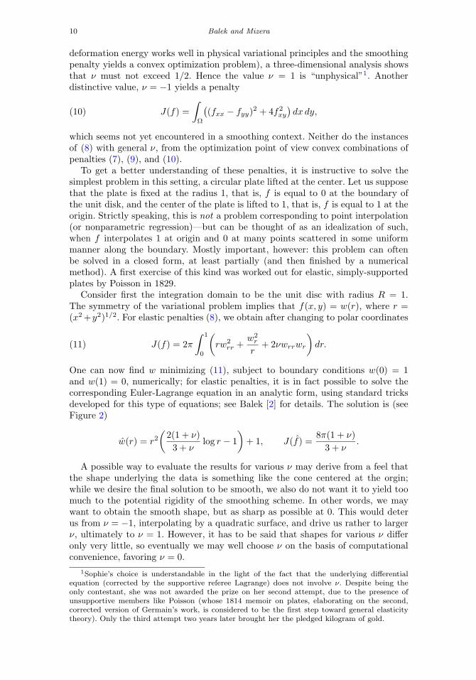
deformation energy works well in physical variational principles and the smoothingpenalty yields a convex optimization problem), a three-dimensional analysis showsthat ν must not exceed 1/2. Hence the value ν = 1 is “unphysical”1. Anotherdistinctive value, ν = −1 yields a penalty

(10) J(f) =

$

Ω

"(fxx − fyy)2 + 4f2

xy

#dx dy,

which seems not yet encountered in a smoothing context. Neither do the instancesof (8) with general ν, from the optimization point of view convex combinations ofpenalties (7), (9), and (10).

To get a better understanding of these penalties, it is instructive to solve thesimplest problem in this setting, a circular plate lifted at the center. Let us supposethat the plate is fixed at the radius 1, that is, f is equal to 0 at the boundary ofthe unit disk, and the center of the plate is lifted to 1, that is, f is equal to 1 at theorigin. Strictly speaking, this is not a problem corresponding to point interpolation(or nonparametric regression)—but can be thought of as an idealization of such,when f interpolates 1 at origin and 0 at many points scattered in some uniformmanner along the boundary. Mostly important, however: this problem can oftenbe solved in a closed form, at least partially (and then finished by a numericalmethod). A first exercise of this kind was worked out for elastic, simply-supportedplates by Poisson in 1829.

Consider first the integration domain to be the unit disc with radius R = 1.The symmetry of the variational problem implies that f(x, y) = w(r), where r =(x2 +y2)1/2. For elastic penalties (8), we obtain after changing to polar coordinates

(11) J(f) = 2π

$ 1

0

&rw2

rr +w2

r

r+ 2νwrrwr

'dr.

One can now find w minimizing (11), subject to boundary conditions w(0) = 1and w(1) = 0, numerically; for elastic penalties, it is in fact possible to solve thecorresponding Euler-Lagrange equation in an analytic form, using standard tricksdeveloped for this type of equations; see Balek [2] for details. The solution is (seeFigure 2)

w(r) = r2

&2(1 + ν)

3 + νlog r − 1

'+ 1, J(f) =

8π(1 + ν)

3 + ν.

A possible way to evaluate the results for various ν may derive from a feel thatthe shape underlying the data is something like the cone centered at the orgin;while we desire the final solution to be smooth, we also do not want it to yield toomuch to the potential rigidity of the smoothing scheme. In other words, we maywant to obtain the smooth shape, but as sharp as possible at 0. This would deterus from ν = −1, interpolating by a quadratic surface, and drive us rather to largerν, ultimately to ν = 1. However, it has to be said that shapes for various ν differonly very little, so eventually we may well choose ν on the basis of computationalconvenience, favoring ν = 0.

1Sophie’s choice is understandable in the light of the fact that the underlying differentialequation (corrected by the supportive referee Lagrange) does not involve ν. Despite being theonly contestant, she was not awarded the prize on her second attempt, due to the presence ofunsupportive members like Poisson (whose 1814 memoir on plates, elaborating on the second,corrected version of Germain’s work, is considered to be the first step toward general elasticitytheory). Only the third attempt two years later brought her the pledged kilogram of gold.

Mechanical models in nonparametric regression 11

Fig 2. The sections of solutions (the domain of integration being the disc with radius R = 1) forν = −1, 0, 0.42 and also the value ν = 1, somewhat put forward already by Sophie Germain (left).

The recognition of the potential of elastic considerations in the interpolation andsmoothing of data dates back at least to Sobolev in 1950’s. The functional mini-mized in the variational problem involving a penalty like (7) is quadratic: the Euler-Lagrange equation is thus linear, the solutions have the superposition property andform a linear space—for fixed values of covariates (xi, yi) a finite-dimensional one.The structure of this linear space is that of a Hilbert space, which opens a pos-sibility to construct solutions via reproducing kernels. Those were introduced inthe smoothing context by Wahba [35], and became popular in the recent statisticalmachine learning literature—where they opened a whole new range of new pos-sibilities, in which penalties are often secondary to kernels, and the properties ofthe resulting solutions are inferred rather in an intuitive fashion; see, for instance,Scholkopf and Smola [29].

From the physical point of view, the domain of integration Ω is naturally de-termined by the solid body represented by f ; consequently, it naturally comes asbounded. In the smoothing context, the domain of integration is inessential in theunivariate case, where the same results are obtained for any Ω containing all ui. Inthe bivariate case, the choice of the domain influences the solution, and thus maybecome an undesirable detail—unless the smoothing domain comes naturally fromthe specification of the problem, as for instance in Ramsay [27].

If we enlarge the integration domain in our radial example, for simplicity stillretaining it a disc but now with radius R > 1, the shape of the plate becomesdifferent. In particular, for ν = 0 we have

(12) w(r) =

(r2(p log r − 1) + 1, when r ≤ 1,

−p log r + (p − 1)"r2 − 1

#, when 1 < r ≤ R,

with p = (1 + (2R)−2)−1, the optimal value of the penalty equal to 4πp. Theresulting shapes can be seen in the left panel of the Figure 3; the tendency withincreasing R is similar to that observed with increasing ν.

The necessity to deal with the integration domain was overcome by the ideal-ization idea of Harder and Desmarais [13], perfected by Duchon [9] and Meinguet[24]. They demonstrated that it is possible to take Ω to be the entire R2, and sub-sequently obtained expressions for the basic functions in closed form; this substan-tially facilitates the application of Hilbert-space methods, and reduces the wholeproblem to a system of linear equations. See also Wahba [35]. The resulting tech-nology became a standard part of the numerical and statistical methodology—thedenomination “thin-plate spline” now assumes, as a rule, implicitly Ω = R2. Spe-cial adjectives are added rather otherwise: for example, Green and Silverman [12]

12 Balek and Mizera

Fig 3. Elastic and plastic penalties on enlarged domains. Left panel shows the sections of solutionsfor ν = 0, and R = 1, 1.8, +∞. Right panel shows the sections of the solution of the interpolationproblem for the plastic penalty with κ = 0, on a disc with radius R equal to 1, 1.375, 1.660, 1.715.

speak about “finite-window thin-plate splines” in case when Ω is bounded. Theymotivate their interest in such a variant by the desire to achieve better behaviornear the boundary of the data cloud (which may be unduly influenced by adoptingthe unbounded domain).

In the radial example, the thin-plate spline solution is obtained by letting R →+∞, making p → 1 in (12). This yields

w(r) =

(r2(log r − 1) + 1, when r ≤ 1,

− log r, when r > 1,

with the optimal penalty 4π. Note that the solution inside the unit disc is equal tothat with ν = 1 and R = 1; however, it can be shown (via the Green theorem) thatthe solution, as whole, does not depend on ν in this case (returning in this casesomewhat to the perspective of Sophie Germain).

5. Plastic penalties

As already mentioned, the difference between elasticity and plasticity is reversibility—here understood in its apparent, macroscopic2 expression: if the body returns toits original configuration, the deformation is elastic; if it does not, then it is (atleast partially) plastic.

To identify our position within existing plasticity theories, we need to invokeseveral notions, pretty much exclusively for the sake of this paragraph. Typically,increasing the forces applied to a body first causes an elastic deformation—unlesswe face an instance of rather idealized behavior, “rigid plasticity”—until a criticalvalue called yield limit is reached, marking the transition to the subsequent plasticbehavior. A theory describing the plastic regime in its initial stages, in a manneranalogous to elasticity theory, is known as the deformation theory of plasticity.It relates stress to the deformation in a way that views plasticity as a kind ofnonlinear elasticity. The version of this theory for “perfectly plastic rigid-plasticbodies” provides a physical model for certain alternative penalties in nonparametric

2On the microscopic level, the irreversibility originates in the motion of dislocations in the crys-tallic latice of the body (see Landau and Lifschitz [22]), which is not related to the irreversibilityof thermodynamic processes described by Bolzmann’s H-theorem, but is rather a consequence ofthe fact that the energy of the material contains many local minima close to each other; in anycase, this aspect is irrelevant for what we are pursuing here.

Mechanical models in nonparametric regression 13

regression. “Perfect plasticity” refers here to an idealized behavior characterizedby the absence of so-called hardening, the necessity to increase stress to producefurther plastic deformations. The deformation theory can be extended to capturethe latter phenomenon, but its principal shortcoming is its lack of explanation forirreversibility—this motivated other theories of plasticity, in particular incremental,or flow plasticity theory; see Kachanov [16]. All simplifications notwithstanding, thedeformation theory of perfect rigid plasticity is extensively employed in engineering,as the basis of so-called limit analysis—the study of limit loads when plasticitytakes over (and the subsequent deformations). Simply put, the deformation theoryis capable to tell us when structures like roofs and bridges are prone to collapse.

As an illustration, consider again the beam with aligned load. If we increase thestress, the beam extends according to the law δ = σ/E; however, after the stressreaches the yield limit E , the beam extends further with the stress staying un-changed. Then, after the beam has been stretched long enough, we need to increasethe stress again in order that the dilation increases. The three stages described hereare respectively elastic deformation, yielding and hardening. “Rigid plastic” are theidealized materials that skip the first stage; “perfectly plastic” are those that skipthe third one. Note that in addition to the constitutive equation δ = σ/E, for aperfectly plastic beam we have also the constitutive inequality σ ≤ E , which mustbe satisfied when the beam is in equilibrium.

For a rigid-plastic beam, the calculation of deformation energy is even simplerthan for an elastic beam. By integrating the stress E over the values of δ rangingfrom 0 to ∆ we find that the deformation energy is E∆. If the load acts in theopposite direction, so that the beam is compressed and the relative dilation isnegative, the energy density is −E∆. Thus, the general expression for the energydensity is E|∆|. Consider now a rigid-plastic rod that is neither entirely stretchednor compressed, but bent. Again, as in an elastic rod, the layers on one side of thecentral surface are stretched and the layers on the other side of the central surfaceare compressed, so that the mean dilation is zero; however, the mean magnitudeof the dilation is nonzero, and from the geometry of the problem it follows that itis proportional to the magnitude of the curvature of the beam, or |f ′′| for smalldeflections. In this way we find that the deformation energy of the rod is given by(5).

The principal concept we will work with from now on, the cornerstone of thedeformation theory, is the yield criterion. In two dimensions, it is represented byan orthogonal-similarity-invariant norm ∥ · ∥ on 2×2 symmetric matrices. The factthat any such norm can be fully characterized in terms of eigenvalues leads toits two-dimensional representation via the so-called yield surface—which visualizes(Figure 4), in the space of eigenvalues, the constitutive inequality

(13) ∥M∥ ≤ µ;

here M is the moment matrix (related to stress) and µ is a threshold value: theplate is deformed elastically or remains flat if ∥M∥ < µ, and may be deformedplastically if ∥M∥ = µ. The constitutive equation is subsequently obtained fromthe postulate that the Hessian, H, is proportional (with negative proportionalityconstant) to the gradient of ∥M∥. Consistently with the general concept of dualityin the mechanics of deformable bodies, discussed in Temam [32], the ensuing plasticdeformation energy corresponding to (13) is

(14)

$

Ω∥H∥∗ dx dy,

14 Balek and Mizera

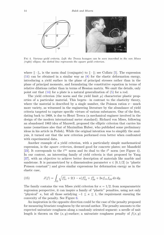
Fig 4. Various yield criteria. Left: the Tresca hexagon can be seen inscribed in the von Mises(right) ellipse; the dotted line represents the square yield criterion.

where ∥ · ∥∗ is the norm dual (conjugate) to ∥ · ∥; see Collatz [5]. The expression(14) can be obtained in a similar way as (8) for the elastic deformation energy,introducing a yield surface in the plane of principal stresses rather than in theplane of principal moments, and formulating the constitutive equation in terms ofrelative dilations rather than in terms of Hessian matrix. We omit the details, onlypoint out that (14) for a plate is a natural generalization of (5) for a rod.

The yield criterion (the norm and the yield limit µ) characterize plastic prop-erties of a particular material. This begets—in contrast to the elasticity theory,where the material is described by a single number, the Poisson ration ν—muchmore variety, as witnessed in the engineering literature by the abundance of yieldcriteria targeted to capture specific virtues of various substances. One of the first,dating back to 1868, is due to Henri Tresca (a mechanical engineer involved in thedesign of the modern international meter standard). Richard von Mises, followingan abandoned 1863 idea of Maxwell, proposed the elliptic criterion that carries hisname (sometimes also that of Maximilian Huber, who published some preliminaryideas in his article in Polish). While the original intention was to simplify the anal-ysis, it turned out that the new criterion performed even better when confrontedwith experimental data.

Another example of a yield criterion, with a particularly simple mathematicalexpression, is the square criterion, deemed good for concrete plates; see Mansfield[23]. It corresponds to the ℓ∞ norm and its dual to the ℓ1 norm (see Figure 4).In our context, an interesting family of yield criteria is that proposed by Yang[37], with an objective to achieve better description of materials like marble andsandstone. It is parametrized by a dimensionless parameter κ ∈ [0, 1/2] (a “plasticPoisson constant”) and gives similar expressions for deformation energy as in theelastic case,

(15) J(f) =

$

Ω

)f2

xx + 2(1 − κ)f2xy + f2

yy + 2κfxxfyy dx dy.

The family contains the von Mises yield criterion for κ = 1/2; from nonparametricregression perspective, it can inspire a family of “plastic” penalties, using not only“physical” κ, but all those satisfying −1 ≤ κ ≤ 1, the requirement ensuring theconvexity of the penalty. See Figure 6.

An inspiration in the opposite direction could be the case of the penalty proposedfor measuring bivariate roughness by the second author. The penalty amounts to theexpected univariate roughness along a randomly oriented segment: a needle of unitlength is thrown on the (x, y)-surface; a univariate roughness penalty of f(x, y)

Mechanical models in nonparametric regression 15

Fig 5. “Buffon penalty” norm (left), and the associated yield criterion (right).

evaluated for (x, y) along the needle; and the average of many such evaluationstaken. For obvious reasons, this measure of roughness was dubbed “Buffon penalty”.The associated matrix norm in the expression (14) bears some similarity with aspectral norm: if the matrix is interpreted as a quadratic form, then the spectralnorm returns its maximal value over vectors with unit norm, while the “Buffonnorm” returns the average value (with respect to the uniform distribution over theunit sphere of directions). The corresponding norm and its dual are visualized inFigure 5; the yield criterion appears to be a sort of merge between those of vonMises and Tresca.

For plastic penalties with general norms, the solutions of the radial example, thecircular plate lifted at the center, are again radial functions and can be expressedin terms of polar coordinates. For instance, for the family (15) we have

(16) J(f) = 2π

$ R

0

"r2w2

rr + w2r + 2κrwrrwr

#1/2dr.

However, the optimal w have to be generally computed numerically, only certainspecial cases can be solved in closed form. The integration domains are again discswith radius R. The easiest case is R = 1 and κ = 0, when w(r) = 1− r, for r goingfrom 0 to 1. In fact, this is a special case: for any R ∈ [1, Rcrit) and any κ, there isa unique q ∈ [0, 1) such that

w(r) = 1 − r1−q for 0 ≤ r ≤ 1,

and these solutions can be extended to r ranging from 1 to R; we omit the details.Unfortunately, the case R = +∞, the extension of the integration domain Ω to thewhole R2, does not work out here as in the elastic case: starting with some criticalvalue Rcrit (which appears to be 1.765) of R (that is, not asymptotically), thesolutions degenerate: they are equal to 1 at 0 and to 0 elsewhere. The right panel ofFigure 3 clearly indicates this tendency, showing the sections with q = 0.4, 0.8, 0.9,corresponding approximately to R = 1.375, 1.660, 1.715.

Albeit the introduction of total variation penalties (6) by Koenker, Ng and Port-noy [19] in nonparametric regression, and by Rudin, Osher and Fatemi [28] in im-age reconstruction predated the recent interest in regularization with ℓ1 penalties,it may be appealing to compare the latter, made popular by Chen, Donoho andSaunders [4] and Tibshirani [33], to the plastic penalties discussed here. Certainplain explanations (and new labels like “fused lasso” for total-variation regulariza-tion [11]) are particularly inviting in the univariate case: the piecewise-linear form

16 Balek and Mizera

of the solutions for the penalty (5) may be interpreted as a consequence of thetendency of the absolute value to pick up “sparse” solutions for f ′′. It is only thebivariate case where the differences stand more out (although even there is a pos-sibility to interpret the plastic penalties in the “group lasso” vein). On the otherhand, there is some analogy to sparsity aspects even there, demonstrating itselfin the nonparametric regression context as the possibility of capturing qualitativefeatures like spikes and edges, without oversmoothing the relevant information; seeDavies and Kovac [6] for an overview of this aspect.

In the ℓ1 context, however, the relevant linear spaces of solutions are no longerHilbert spaces; the possibility of using reproducing kernels is lost, and with it possi-bly one potential attraction of unbounded integration domains. Even in the ℓ2 con-text, solving linear equations may not be that straightforward anymore when thesystem is large—unless its matrix is sparse, exhibiting relatively only few nonzeroentries. The matrices arising in closed-form solutions obtained by reproducing ker-nels are non-sparse—and there does not seem to be any workaround for this; seeSilverman [30], Wood [36]. A possible way out is to trade the “exact” solution for anapproximate one, but with a sparse linear system involved in its computation; whichis the case, for instance, in the finite-element implementations by Hegland, Robertsand Altas [15], Duchamp and Stuetzle [8], Ramsay [26], and others. The algorithmsthus return back to that of boundary value problems, where the idealization of Ωto R2 is not any longer a necessity.

6. Extensions and ramifications

In the final section, we would like to touch briefly some other aspects where phys-ical analogies may or might provide some guidance. The first of them concernsblends—convex combinations of several penalties. In the discussion of the resultsof smoothing with elastic penalties for the radial example we noted that, from acertain perspective, it may be desirable to have those fits as “sharp” as possibleat 0. As it was felt that purely elastic penalties may not sufficiently achieve thisobjective, several solutions were proposed to this end.

One possibility is to use the plastic penalty, which in the radial example withR = 1 yields the “ideal” conic shape of the fit. However, its dependence on the inte-gration domain, impossibility of an idealized extension to the unbounded domain,and in particular, the lack of Hilbert-space methods for finding solutions, motivatedso-called thin-plate splines with tension. Recall that in our mechanic deliberations,the thin plate was supposed only to bend, not to stretch. In a more realistic sit-uation involving some stretching and some bending, the physical model results ina “blended” penalty: for instance, a convex combination of (7) and the Dirichletpenalty

(17) J(f) =

$

Ω

"f2

x + f2y

#dx dy.

The latter coresponds in mechanics not to an elastic or plastic deformation of anon-stretching thin plate, but instead to the deformation of a membrane: an elasticplate where stretching is dominant. It is known that it is not possible to use (17) insmoothing by itself—an instance of a broader phenomenon of increasing need forderivatives in regularization penalties, related in some sense to the embedding the-ory of functional spaces of Sobolev type, an intuitive explanation of which is given interms of the radial interpolation example on page 160 of Green and Silverman [12].

Mechanical models in nonparametric regression 17

Fig 6. Plastic splines vs. thin-plate splines with tension. Left: plastic penalties (15), with κ =1, 1/2, 0,−1/2,−1. Right: convex combinations of thin-plate spline penalty (7) with tension termweighted 0, 0.9, 0.99, 0.999.

In the radial example minimizing (17), the solution degenerates—more precisely, itdoes not exist. However, as can be seen in the right panel of Figure 6, adding evena small portion of an elastic penalty acts as a regularizer, and a fair proportion of“tension” yields more pronounced peak in the solution of the radial interpolation(an excessive one draws it closer to the funnel-like degeneracy). Moreover, the so-lutions in Figure 6 can be actually obtained in closed form using modified Besselfunctions, via (11) and the analogous expressions for (17); thin-plate splines withtension proposed by Franke [10] actually provide quite accurate approximation tothis solution, especially for higher tension weights.

A possible suggestion in a similar direction is to regularize plastic by an elasticpenalty. A way that would be analogous to the approach of thin-plate splines withtension is to consider a convex combination of a plastic and elastic penalty. Theresults can be seen in the left panel of Figure 7; it turns out that the regularizingeffect (and thus a possibility of extending the whole formulation to the unboundeddomain) is achieved by a quite small proportion of the elastic penalty (in fact,some optimization algorithms may already exhibit a similar regularization effectspontaneously, due to the nature of the approximations involved). It may be ofinterest that a similar idea of combining ℓ1 and ℓ2 penalty appeared in recently ina different context under the name “elastic net” [38].

Fig 7. Elastoplastic penalties. Left: total-variation penalty (6) regularized via the convex combi-nation with thin-plate spline penalty (7) weighted 0.1, 0.01, 0.001, on the disc with radius R = 2.3.Right: elastoplastic penalty with ι = 0 and β = 20, 2.845, 1, 0.2. The dotted line in the left panelis the result for the total-variation penalty when R = 1, which in the right panel almost coincideswith the fit for β = 2.845.

18 Balek and Mizera

It would be tempting to call the blended penalty “elastoplastic”; however, ifa situation—corresponding even more to reality—when there is some plastic andsome elastic behavior in bending, is approached from the physical point of view,the object we arrive to is Hencky’s plate, the perfectly plastic elastoplastic platedescribed by the deformation theory. In such bodies, a pure elastic deformationtakes place if the stresses lay inside the yield diagram, and a combined elastic andplastic deformation possibly takes place if the stresses are placed at the surface ofthe yield diagram. Furthermore, the plastic part of deformation is the same as inrigid-plastic bodies. The leads to a family of penalties

J(f) =

$

Ωϕ*)

f2xx + 2(1 − ι)f2

xy + f2yy + 2ιfxxfyy

+dx dy,

generalizing, for ι = ν = κ, the elastic penalties (8), with ϕ(u) = u2, and plasticpenalties (15), with ϕ(u) = |u|, via a function ϕ known in statistics as the Huberfunction, equal to u2/2 for |u| ≤ β, and to β|u| − β2/2 otherwise; the parameter βis determined by the yield criterion. The results for the radial example, for ι = 0and various choices of β, can be seen in the right panel of Figure 7.

References

[1] Arnol’d, V. I. (1990). Huygens and Barrow, Newton and Hooke. Birkhauser,Basel.

[2] Balek, V. (2011). Mechanics of plates. http://xxx.lanl.gov/abs/1110.2050.[3] Bookstein, F. L. (1991). Morphometric Tools for Landmark Data: Geometry

and Biology. Cambridge University Press, Cambridge.[4] Chen, S. S., Donoho, D. L. and Saunders, M. A. (1998). Atomic decom-

position by basis pursuit. SIAM J. Sci. Comput. 20 33–61.[5] Collatz, L. (1966). Functional Analysis and Numerical Mathematics. Aca-

demic Press, New York.[6] Davies, P. L. and Kovac, A. (2001). Local extremes, runs, strings and

multiresolution (with discussion). Ann. Statist. 29 1–65.[7] Dryden, I. L. and Mardia, K. V. (1998). Statistical Shape Analysis. Wiley,

Chichester.[8] Duchamp, T. and Stuetzle, W. (2003). Spline smoothing on surfaces. Jour-

nal of Computational and Graphical Statistics 12 354–381.[9] Duchon, J. (1976). Interpolation des fonctions de deux variables suivant le

principe de la flexion des plaques minces. R.A.I.R.O., Analyse numerique 101–13.

[10] Franke, R. (1985). Thin plate splines with tension. Computer Aided Geo-metric Design 2 85–95.

[11] Friedman, J., Hastie, T., Hofling, H. and Tibshirani, R. (2007). Path-wise coordinate optimization. Ann. Appl. Statist. 1 302–332.

[12] Green, P. J. and Silverman, B. W. (1994). Nonparametric Regression andGeneralized Linear Models: A Roughness Penalty Approach. Chapman andHall, London.

[13] Harder, R. L. and Desmarais, R. N. (1972). Interpolation using surfacesplines. J. Aircraft 9 189–191.

[14] He, X., Ng, P. and Portnoy, S. (1998). Bivariate quantile smoothingsplines. J. R. Statist. Soc. B 60 537–550.

[15] Hegland, M., Roberts, S. and Altas, I. (1998). Finite element thin platesplines for surface fitting. In: Computational Techniques and Applications:

Mechanical models in nonparametric regression 19

CTAC 97 (J. Noye, M. Teubner and A. Gill, eds.). World Scientific, Singa-pore.

[16] Kachanov, A. M. (1956). Osnovy Teorii Plastichnosti. GITTL, Moscow.[17] Koenker, R. and Mizera, I. (2002). Elastic and plastic splines: Some ex-

perimental comparisons. In Statistical Data Analysis Based on the L1-Normand Related Methods (Y. Dodge, ed.) 405–414. Birkhauser, Basel.

[18] Koenker, R. and Mizera, I. (2004). Penalized triograms: Total variationregularization for bivariate smoothing. J. R. Statist Soc. B 66 1681–1736.

[19] Koenker, R., Ng, P. and Portnoy, S. (1994). Quantile smoothing splines.Biometrika 81 673–680.

[20] Lakes, R. (1987). Foam structures with a negative Poisson’s ratio. Science27 1038–1040.

[21] Landau, L. D. and Lifshitz, Y. M. (1986). Theory of Elasticity. PergamonPress, London. [Third English edition, revised and enlarged by E. M. Lif-shitz, A. M. Kosevich and L. P. Pitaevskii; translated from Teoriia uprugosti,Moskva, Nauka, 1986, by J. B. Sykes and W. H. Reid].

[22] Mammen, E. and van de Geer, S. A. (1997). Locally adaptive regressionsplines. Ann. Statist. 25 387–413.

[23] Mansfield, E. H. (1957). Studies in collapse analysis of rigid-plastic plateswith a square yield diagram. Proc. R. Soc. of London A 241 311–338.

[24] Meinguet, J. (1979). Multivariate interpolation at arbitrary points madesimple. J. Appl. Math. Phys. (ZAMP) 30 292–304.

[25] O’Sullivan, F. (1991). Discretized Laplacian smoothing by Fourier methods.J. Amer. Statist. Assoc. 86 634–642.

[26] Ramsay, T. O. (1999). A Bivariate Finite-Element Smoothing Spline Appliedto Image Registration. Queen’s University, Kingston. Thesis.

[27] Ramsay, T. (2002). Spline smoothing over difficult regions. J. R. Statist. Soc.B 64 307–319.

[28] Rudin, L. I., Osher, S. and Fatemi, E. (1992). Nonlinear total variationbased noise removal algorithms. Physica D 60 259–268.

[29] Scholkopf, B. and Smola, A. J. (2002). Learning With Kernels. MIT Press,Cambridge, MA.

[30] Silverman, B. W. (1985). Some aspects of the spline smoothing approach tonon-parametric regression curve fitting. J. R. Statist. Soc. B 47 1–52.

[31] Small, C. G. (1996). The Statistical Theory of Shape. Springer-Verlag, NewYork.

[32] Temam, R. (1983). Problemes Mathematiques en Plasticite. Bordas, Paris.[English translation: Mathematical Problems in Plasticity, Bordas, Paris,1985].

[33] Tibshirani, R. (1996). Regression shrinkage and selection via the lasso. J. R.Statist. Soc. B 58 267–288.

[34] Timoshenko, S. P. and Woinowsky-Krieger, S. (1959). Theory of Platesand Shells. McGraw-Hill, New York.

[35] Wahba, G. (1990). Spline models for observational data. CBMS-NSF RegionalConference Series in Applied Mathematics. SIAM, Philadelphia.

[36] Wood, S. N. (2003). Thin-plate regression splines. J. R. Statist. Soc. B 6595–114.

[37] Yang, W. H. (1980). A useful theorem for constructing convex yield functions.J. Appl. Mech. 47 301–303.

[38] Zou, H. and Hastie, T. (2005). Regularization and variable selection via theelastic net. J. R. Statist. Soc. B 67 301–320.