mechanical engineering design...
TRANSCRIPT

Mechanical Engineering Design Project
MECH 390
Lecture 10
3/19/2018 Chapter 7-Project Planning 2
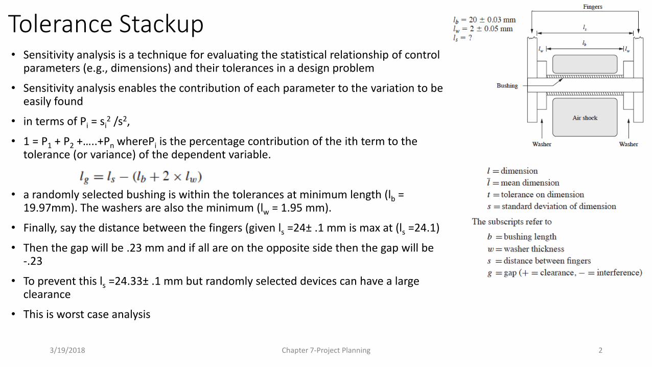
Tolerance Stackup• Sensitivity analysis is a technique for evaluating the statistical relationship of control
parameters (e.g., dimensions) and their tolerances in a design problem
• Sensitivity analysis enables the contribution of each parameter to the variation to be easily found
• in terms of Pi = si2 /s2,
• 1 = P1 + P2 +…..+Pn wherePi is the percentage contribution of the ith term to the tolerance (or variance) of the dependent variable.
• a randomly selected bushing is within the tolerances at minimum length (lb = 19.97mm). The washers are also the minimum (lw = 1.95 mm).
• Finally, say the distance between the fingers (given ls =24± .1 mm is max at (ls =24.1)
• Then the gap will be .23 mm and if all are on the opposite side then the gap will be -.23
• To prevent this ls =24.33± .1 mm but randomly selected devices can have a large clearance
• This is worst case analysis

3/19/2018 Chapter 7-Project Planning 3
Tolerance Stackup• More accurate analysis is to do this statistically
• stack-up problem composed of n components, each with mean length li and tolerance ti (assumed symmetric about the mean), with i = 1, …, n. If one dimension is identified as the dependent parameter (the gap), then its mean and SD can be found by prev eqn
• And in terms of tolerance where S = t/3 If given ls =24± .1 mm
These results show that there is, on the average, no gap and the tolerance on itis 0.126 mm. if a clearance of .07 and interference of .03 is allowed, what % will meet the requirements?using standard normal probability methods the shaded area represents 71% of the assemblies. This means that 29% of thetime either the assembly people will have trouble assembling the device (24%) or the welds will be overstressed (5%).

3/19/2018 Chapter 7-Project Planning 4
Sensitivity analysis• Sensitivity analysis is a technique for evaluating the statistical relationship of control
parameters (e.g., dimensions) and their tolerances in a design problem
• Sensitivity analysis enables the contribution of each parameter to the variation to be easily found
• in terms of Pi = si2 /s2,
• 1 = P1 + P2 +…..+Pn wherePi is the percentage contribution of the ith term to the tolerance (or variance) of the dependent variable.
• Spacing tolerance contributes the biggest towards the gap (63%)
• If a change in dimensioning is needed, it is better on the spacing

3/19/2018 Chapter 7-Project Planning 5
Sensitivity analysis• For non linear relationships as in the tank problem
• Considering some values for r and l. means for point A, 1.21 and 0.87 and stddeviations as shown (in ellipse)
• SD on volume is where
• For the values in this example, ∂V/∂r = 6.61 and ∂V/∂l = 4.60, so Sv = 0.239m3.
• Thus, 99.68% (3Sds) of all the vessels built will have volumes within 0.717m3(3X0.239) of the target 4m3. • (6.612*.052)/.2392 + (4.602*.012)/.2392 =1
• This gives length contribution as 92.3% of variance in volume and radius contribution as 7.6% of variance in volume
• Reduction is variance is achieved by not changing the tolerance, but by changing the nominal values
• If we can find minimum variance for some values of r and l, then we employ the philosophy of robust design
• Also, the %contribution of each radius and length can be calculated
• Looking at point B, where r is 0.5 and l is 5.09,
• For this situation the ∂V/∂r = 16 and ∂V/∂l = 0.78
• Similar calculation to the above, Sv = 0.166m3
• B is of better quality because of 31% reduction in variance of volume
• Also % calculation shows tolerance on r contributes to 94% of variance in volume

3/19/2018 Chapter 7-Project Planning 6
Robust Design by Analysis• The goal was to have V = 4 m3, exactly. (impossible because of tolerances). The “best” is to keep the absolute difference
between V and and 4 m3 as small as possible, in other words, minimize the standard deviation of V with a base value of V= 4 m3.
• Defining the difference between the mean value (3.1416r2l) and the target T (4m3) as the bias, the objective function to be minimized is C = variance + λ × bias where λ is the Lagrange multiplier
• For the tank, the minimizing equation then becomes C = (2πrl)2s2r+ (πr2)2s2
l+ λ(πr2l − T )
• The minimum value of the objective function can now be solved. With known sr and sl (or tr and tl) and a known target T, values for the parameters r and l can be found from the derivatives of the objective function with respect to the parameters and the Lagrange multiplier:
• Thus, for any ratio of the standard deviations or the tolerances, the parameters are uniquely determined for the best (most robust) design. For the values of sr = 0.01 and sl = 0.05, these equations result in r=0.71m and l=2.52 m.
• Using this the sv = 0.138 m3. Comparing this to the results obtained in the sensitivity analysis, 0.239 and 0.165 m3, the improvement in the design quality is evident.
• If the standard deviation is unacceptable, then the next option is to reduce the tolerance on length and radius
3/19/2018 Chapter 7-Project Planning 7
Robust Design by Analysis• The analysis based robust design can be summarized in 3 steps
• Step 1. Establish the relationship between quality characteristics and the control parameters. Also, define a target for the quality characteristic.
• Step 2. Based on known tolerances (standard deviations) on the control variables, generate the equation for the standard deviation of the quality characteristic.
• Step 3. Solve the equation for the minimum standard deviation of the quality characteristic subject to this variable being kept on target.
• For the example, given, Lagrange’s technique was used; other techniques are available, and some are even included in most spreadsheet programs.
• There are usually other constraints on this optimization problem that limit the values of the parameters to feasible levels. For the example given, there could have been limits on the maximum and minimum values of r and l.
• There are some limitations on the method developed here. First, it is only good for design problems that can be represented by an equation.
• In systems in which the relationships between the variables cannot be represented by equations, experimental methods must be used
• Second, the minimizing equation does not allow for the inclusion of constraints in the problem. If the radius, for example, had to be less than 1.0 m because of space limitations, the Equation would need additional terms to include this constraint.

3/19/2018 Chapter 7-Project Planning 8
Robust Design by Testing• It is often impossible to analytically evaluate a proposed design because no mathematical models of the system exist or
the fidelity of those that do are too low. In many cases, even when analysis is possible, the analytical model of the system may not allow determination of the effect of the noise on a proposed design.
• If the system cannot be described in equations, experimental methods need to be used. Here we will use Taguchi method for the tank problem assuming that we do not know the formula for volume of the cylinder. We just know the V = f (r, l).
• To experimentally find dimensions for radius and length, we could begin by building a tank with some best-guess dimensions and then measuring the volume.
• Then, if the volume was too high, we could build new models, one with a smaller radius and another with a shorter length, and then measure the volumes.
• Based on these new measurements, we could try to estimate the dependence of the volume on each of the dimensions and iterate (i.e., patch) our way to the target volume.
• This is the way most experiments are run. This “random walk” toward a solution may require many models, so it is not very efficient.
• Additionally, the solution found could be anywhere on the curve shown in Fig; there is no guarantee that the final design will be the most robust.
• The following steps can overcome these drawbacks.
3/19/2018 Chapter 7-Project Planning 9
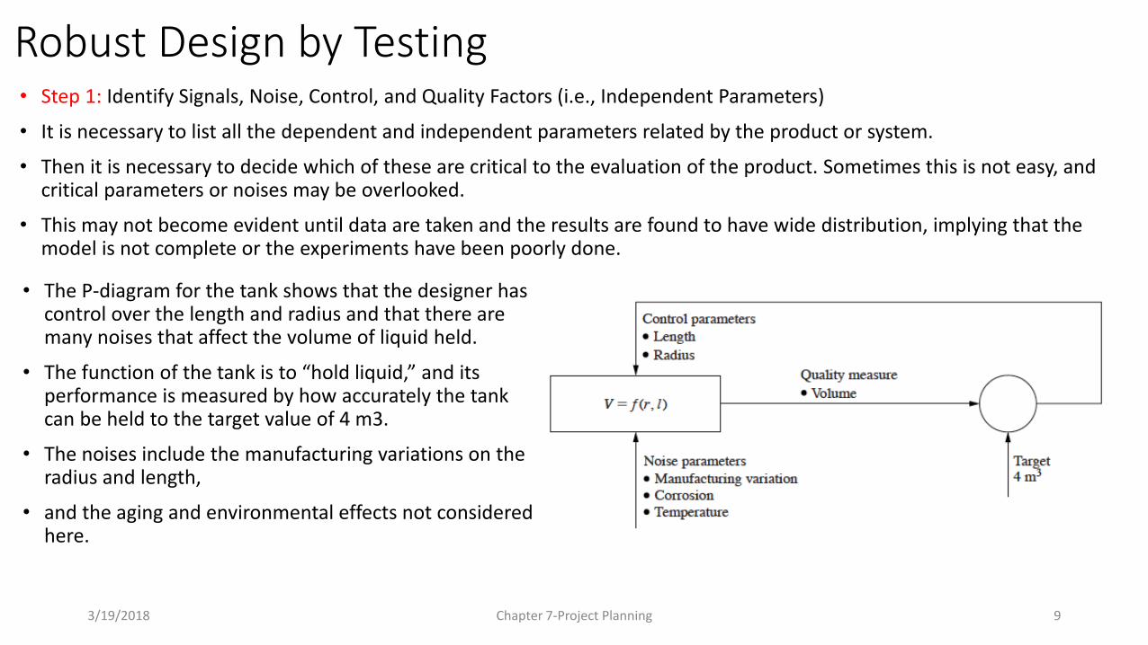
Robust Design by Testing• Step 1: Identify Signals, Noise, Control, and Quality Factors (i.e., Independent Parameters)
• It is necessary to list all the dependent and independent parameters related by the product or system.
• Then it is necessary to decide which of these are critical to the evaluation of the product. Sometimes this is not easy, and critical parameters or noises may be overlooked.
• This may not become evident until data are taken and the results are found to have wide distribution, implying that the model is not complete or the experiments have been poorly done.
• The P-diagram for the tank shows that the designer has control over the length and radius and that there are many noises that affect the volume of liquid held.
• The function of the tank is to “hold liquid,” and its performance is measured by how accurately the tank can be held to the target value of 4 m3.
• The noises include the manufacturing variations on the radius and length,
• and the aging and environmental effects not considered here.
3/19/2018 Chapter 7-Project Planning 10
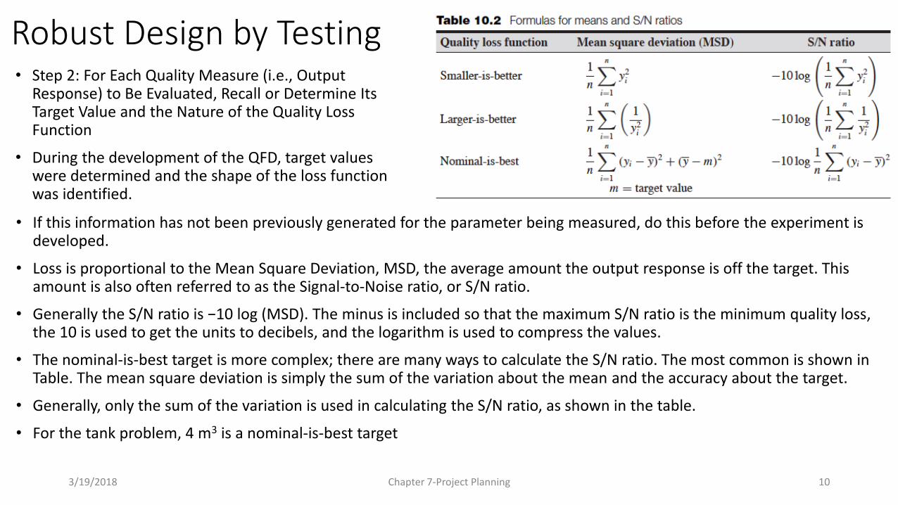
Robust Design by Testing• Step 2: For Each Quality Measure (i.e., Output
Response) to Be Evaluated, Recall or Determine Its Target Value and the Nature of the Quality Loss Function
• During the development of the QFD, target values were determined and the shape of the loss function was identified.
• If this information has not been previously generated for the parameter being measured, do this before the experiment is developed.
• Loss is proportional to the Mean Square Deviation, MSD, the average amount the output response is off the target. This amount is also often referred to as the Signal-to-Noise ratio, or S/N ratio.
• Generally the S/N ratio is −10 log (MSD). The minus is included so that the maximum S/N ratio is the minimum quality loss, the 10 is used to get the units to decibels, and the logarithm is used to compress the values.
• The nominal-is-best target is more complex; there are many ways to calculate the S/N ratio. The most common is shown in Table. The mean square deviation is simply the sum of the variation about the mean and the accuracy about the target.
• Generally, only the sum of the variation is used in calculating the S/N ratio, as shown in the table.
• For the tank problem, 4 m3 is a nominal-is-best target

3/19/2018 Chapter 7-Project Planning 11
Robust Design by Testing
• Step 3: Design Experiment
• Suppose there are n control factors and data are taken for each at two different settings, there are m noise variables also to be tested at two levels, and, for accuracy, there are k repetitions to be run for each condition. Then there are k · 2n · 2m
experiments to perform.
• If there are two control factors, two noises, and three repetitions for each condition, then there are 48 output responses to be recorded. To keep the number of experiments to a reasonable level, there are statistically based techniques for choosing a subset of experiments to run.
• Table shows a layout for an experiment with two control factors, each tested at two levels with two noises also each at two levels. The results for the output response, F, are shown for the 16 experiments.
• If, for example, there were three repetitions of experiment F2112 (control factor 1 at level 2, control factor 2 at level 1, noise 1 at level 1, and noise 2 at level 2), then there would be three F2112 values.
• If all the experiments were run three times, there would be 48 experiments. The mean value and S/N ratio for each control-factor combination are calculated in the last two columns.

3/19/2018 Chapter 7-Project Planning 12
Robust Design by Testing
• Step 3: Design Experiment
• If there are two control factors, two noises, and three repetitions for each condition, then there are 48 output responses to be recorded. To keep the number of experiments to a reasonable level, there are statistically based techniques.
• Table shows a layout for an experiment with two control factors, each tested at two levels with two noises also each at two levels. The results for the output response, F, are shown for the 16 experiments.
• If, for example, there were three repetitions of experiment F2112 (control factor 1 at level 2, control factor 2 at level 1, noise 1 at level 1, and noise 2 at level 2), then there would be three F2112 values.
• If all the experiments were run three times, there would be 48 experiments. The mean value and S/N ratio for each control-factor combination are calculated in the last two columns.
• For the tank problem, experimental models are built to enable accurate setting of the length and radius.
• In Table values of r = 0.5 and r = 1.5. l=0.5 and 5.5. The noises are the tolerance levels l = ±0.15 and r=±0.03
• To find the output response for cell F2112, the experiment needs a tank made as precisely as possible with r = 1.53 m and l = 0.35 m.

3/19/2018 Chapter 7-Project Planning 13
Robust Design by Testing
• Two of the mean values are fairly close to the target of 4 m3. This was the result of luck in choosing the starting values for r and l.
• The first set of experiments may not yield satisfactory results. The goal is to maximize the S/N ratio and then bring the mean value on target. For analytical problems, we can find the true maximum (Section 10.9); here we can only estimate when we reach that point.
• For the tank problem, the experiment with the radius r=0.5m and the length l = 5.5 m gives results near the target and with the highest S/N (11.87 dB). The experiments could be stopped here if a mean value of 4.34 m3 is close enough.
• Or the information used to adjust the control parameters. Since experiments with l = 5.5 m resulted in better S/N values, r can be estimated to bring the output to 4 m3. However, how much to change r may not be evident from the data.
• A better idea is to perform experiments by setting new values for r and l around the values found above and taking new readings. This iteration would eventually lead to a volume V = 4 m3 and an S/N ratio of 13.69 at r = 0.71 m and l = 2.52 m, the same values found analytically.
• Step 4: Take and Reduce Data
• The measured volumes of the tank are shown in Table 10.4 along with the calculated values of the mean and nominal-is-best S/N ratio. Mean values and S/N ratios are calculated for repetitions of each set of control and noise conditions.

3/19/2018 14
Optimum Design
• Decision making is all about selecting the best option from small
number of design options
• When number of options increase, selecting the best one is difficult
• Optimization is one such technique that enables identifying the best
design options
• Here we will consider multi stage system design with large but finite
stages and options

3/19/2018 15
Dynamic Programming
• Optimizing design of system configures in stages whose design can be
characterized as a sequence of design decisions
• Transmission power system shown in dwg.
• Power generation at A and Customer at E
• Multiple routing is possible through B C and D
• Cost of going through each of them is given in the
lines in millions of dollars considering topography,
land acquisition etc.
3/19/2018 16
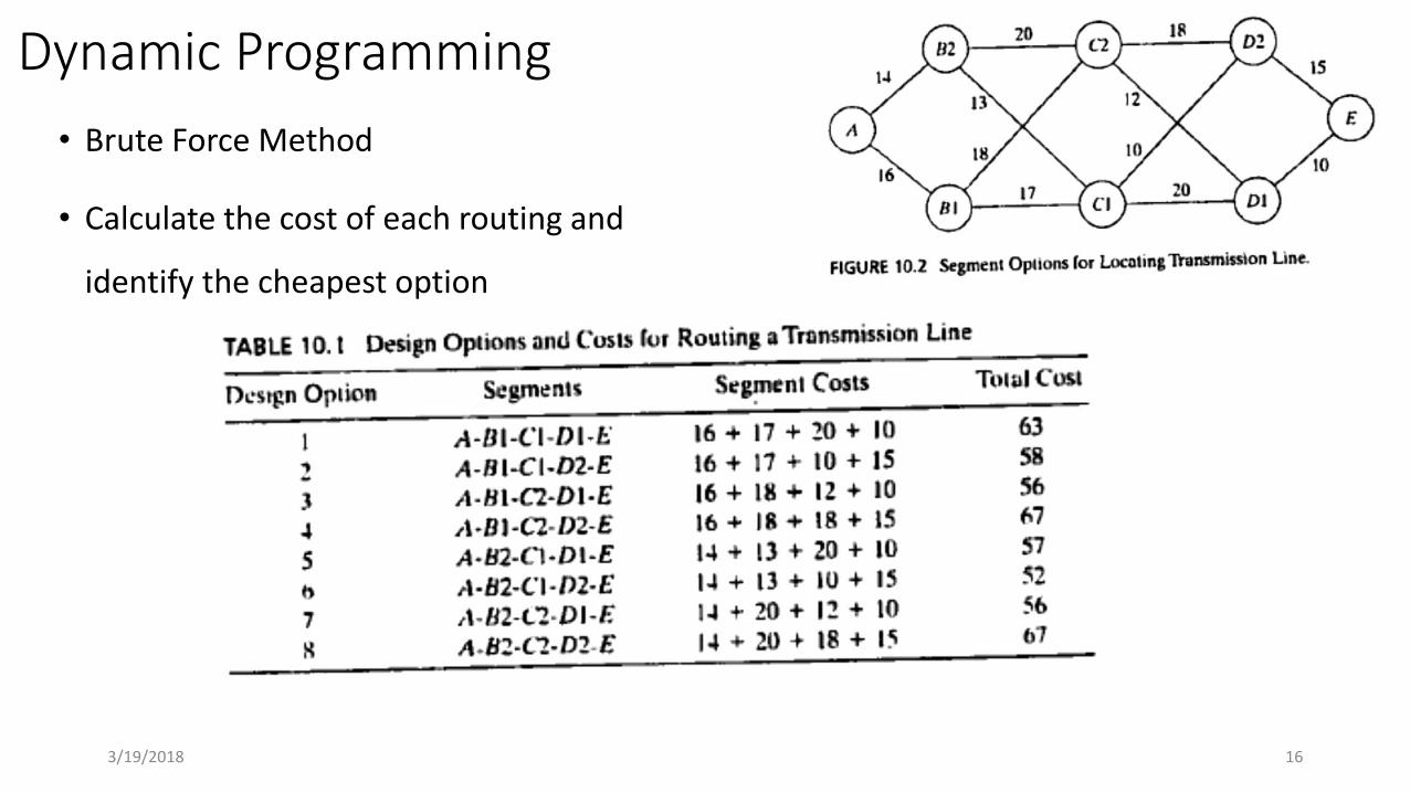
Dynamic Programming
• Brute Force Method
• Calculate the cost of each routing and
identify the cheapest option

3/19/2018 17
Dynamic Programming
• Stage 1 Analysis
• Going backward or forward. Let us go
backward first
• Starting from E, work backwards to A
• D1 and D2 are only possibilities to get to E
3/19/2018 18
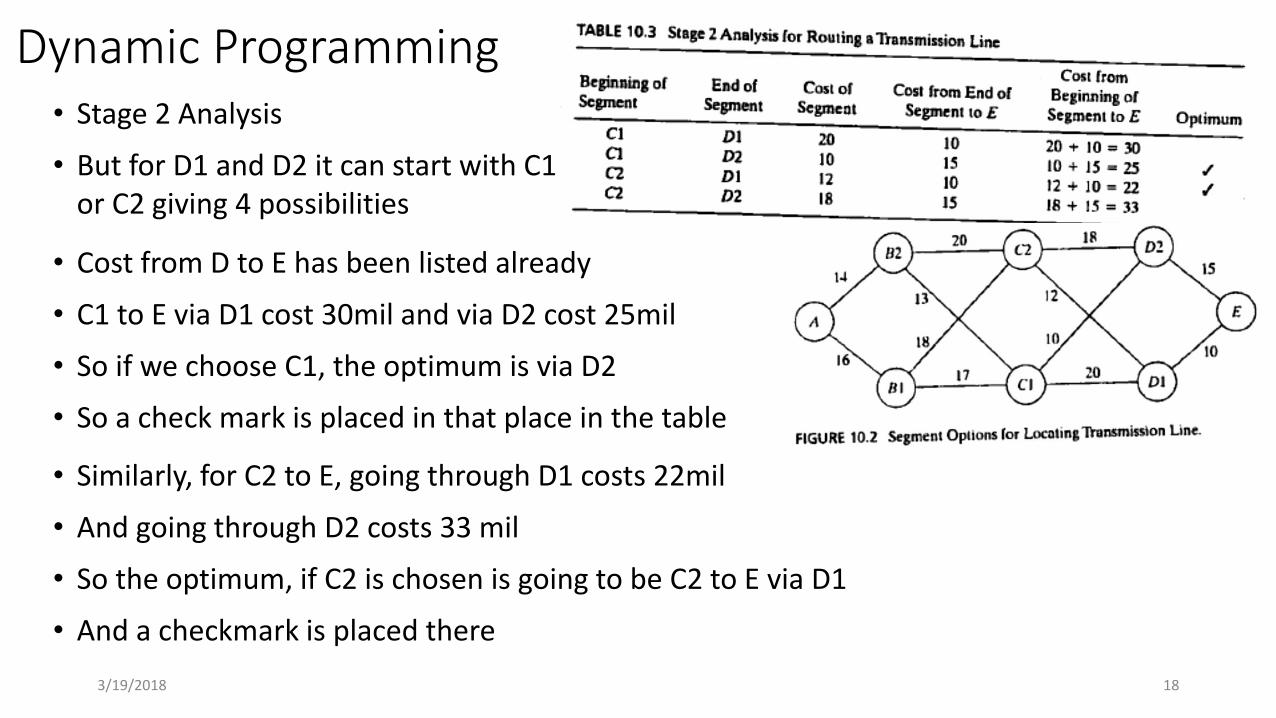
Dynamic Programming• Stage 2 Analysis
• But for D1 and D2 it can start with C1 or C2 giving 4 possibilities
• Similarly, for C2 to E, going through D1 costs 22mil
• And going through D2 costs 33 mil
• So the optimum, if C2 is chosen is going to be C2 to E via D1
• And a checkmark is placed there
• Cost from D to E has been listed already
• C1 to E via D1 cost 30mil and via D2 cost 25mil
• So if we choose C1, the optimum is via D2
• So a check mark is placed in that place in the table

3/19/2018 19
Dynamic Programming• Stage 3 Analysis
• For C1 and C2 it can start with B1 or B2 giving 4 possibilities
• So a check mark is placed in that place in the table
• Similarly, for B2 to E, going through optimized C1 costs 38mil
• And going through C2 costs 42 mil
• And a checkmark is placed there
• Cost from C to E has been optimized for C1 and C2 already in the previous step
• B1 to E via optimized C1 cost 42mil and via optimized C2 cost 40mil
• So if we choose B1, the optimum is via optimized C2

3/19/2018 20
Dynamic Programming• Stage 4 Analysis
• From the optimum values found for routes B1 to E and B2 to E, that we calculated from table 10.4,
• We can find the minimum cost of the routing problem
• There are only two options from A to B via B1 or B2, which has already been optimized.
• As shown in table 10.5, A-B2 will cost the leas at 52 mil
• From table 10.4, optimum is B2-C1 and from table 10.3 it is C1-D2
• D2 E is given in table 10.2
• Hence the optimum route for this problem is A-B2-C1-D2-E
3/19/2018 21
Designing a Pollution Control System• You are designing a chemical filtration to remove pollutants from fluid
• With n number of chemical filters, the design challenge is to distribute chemical among n stages so as to minimize the pollutant remaining in the system as it leaves the stream
• i = 1 to ….n, determines the stages and Pi represent the Pollutant (ppm) entering the stage i and Pi+1 is the amount of pollutant leaving the stage i and entering i+1.
• Our design variable is the amount of chemical used in the individual stage Ci
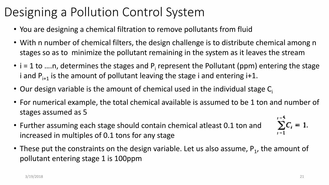
• For numerical example, the total chemical available is assumed to be 1 ton and number of stages assumed as 5
• Further assuming each stage should contain chemical atleast 0.1 ton and increased in multiples of 0.1 tons for any stage
• These put the constraints on the design variable. Let us also assume, P1, the amount of pollutant entering stage 1 is 100ppm

3/19/2018 22
Designing a Pollution Control System• Effectiveness of the ith filter can be modeled as
• where
• And K, k are constants
• Considering k as 0, equation becomes (xi=0)
• This shows that % reduction of pollutant is proportional to the amount of chemical used in that stage. K can be interpreted as the effectiveness of the filer/unit of chemical used
• For a non zero k, has the effect of reducing K. indicating using too much of chemical can clog filter and reduce effectiveness
• For this example let us assume effectiveness K=1 and k=3/200
• Let us identify the number of design options if we have to use brute force
3/19/2018 23
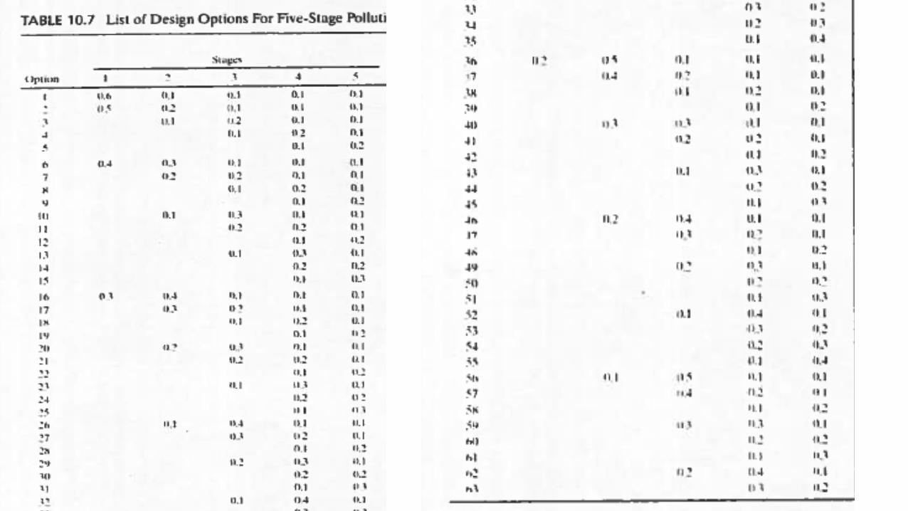
Designing a Pollution Control System• List of design options
• Amount of chemical used in stage 1 is max at 0.6 cos we need at least 0.1 each in subsequent stages
• If we use only 0.5 in stage 1, we have the option of having 0.2 in 2, 3, 4, or 5 and and rest will be 0.1 giving 4 options
• If we reduce in 1 stage and increase in other, there are 126 possible options as shown in table 10.7
• If we have to used brute force, we have to apply equation for each stage (5 times) for 126 options totaling 630 mathematical calculations to find optimum design
• Dynamic programing helps in getting optimum value without examining every option individually


3/19/2018 26
Designing a Pollution Control System• Stage 1 analysis
• Start by constructing table 10.8 to describe stage 1 of the system
• There are six possible choices for stage 1 starting from 0.1 to 0.6 represented by the notation of Qj which shows chemical consumption through stage J
• For stage 1, Q0 is 0, because there is not preceding stage and Q1 is from 0.1 to 0.6
• Third column shows the amount of chemical
• Fourth column (P1) shows the amount of pollutant entering
• And fifth column (P2) shows the amount of pollutant exiting
• P2 is calculated using i as 1 equations 10.1 and 10.2 and values of
• K and k in 10.3
• 0.3 gives the best result, as more reduces the effectiveness
• Still not optimum
3/19/2018 27
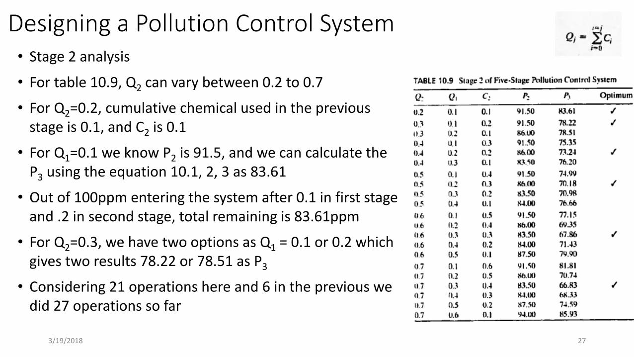
Designing a Pollution Control System• Stage 2 analysis
• For table 10.9, Q2 can vary between 0.2 to 0.7
• For Q2=0.2, cumulative chemical used in the previous stage is 0.1, and C2 is 0.1
• For Q1=0.1 we know P2 is 91.5, and we can calculate the P3 using the equation 10.1, 2, 3 as 83.61
• Out of 100ppm entering the system after 0.1 in first stage and .2 in second stage, total remaining is 83.61ppm
• For Q2=0.3, we have two options as Q1 = 0.1 or 0.2 which gives two results 78.22 or 78.51 as P3
• Considering 21 operations here and 6 in the previous we did 27 operations so far

3/19/2018 28
Designing a Pollution Control System• Stage 3 analysis
• For table 10.10, Q3 can vary between 0.3 to 0.8
• For Q3, carry the best Q2 values that gives better P3
values from previous table
• For Q3=0.4 Q2 can be either 0.2 or 0.3
• If Q2 is 0.2, table 10.9 says P3 is 83.61
• But for Q2 as 0.3, table 10.9 says P3 is 78.22 or 73.24
• We select the least of the values and carry forward in table 10.10
• Calculate P4 for each and check the optimum values
• Considering 21 operations here and 27 in the previous we did 48 operations so far

3/19/2018 29
Designing a Pollution Control System• Stage 4 analysis
• For table 10.11, Q4 can vary between 0.4 to 0.9
• For Q3, carry the best Q3 values that gives better P4
values from previous table
• For Q4=0.5 Q3 can be either 0.3 or 0.4
• If Q3 is 0.3, table 10.10 says P4 is 76.29
• But for Q3 as 0.4, table 10.10 says P4 is 71.32 or 71.08
• We select the least of the values and carry forward in table 10.11
• Calculate P5 for each and check the optimum values

3/19/2018 30
Designing a Pollution Control System• Stage 5 analysis
• Only 6 options since Q5 is 1. So if Q4 is 0.4 C5 should be 0.6 and so on
• Repeat the process for identifying the optimum variable for example if Q4 is 0.5, P5 is 64.53 and 64.73, choose 64.53
• We get the optimum value of 43ppm from table 10.12
• This was achieved using 6+21+21+21+6 =75 operations
• Which is way less than you would use in brute force = 630
• We can work back the values to identify the chemical in each filter

3/19/2018 31
Linear Programming• Here we will look at optimizing engineering design with n ariables x1, x2, ……xn
• These are subject to inequality constraints
• Optimum design is the one that gives combination of design variables such that
• You maximize the objective function without violating the constraints
• Mathematically the linear programing is maximizing the objective function
• Where n is the number of design variables subject to m constraints as in
• Where a and k are constants and know for
• Particular problem and design variable are non negative
3/19/2018 32
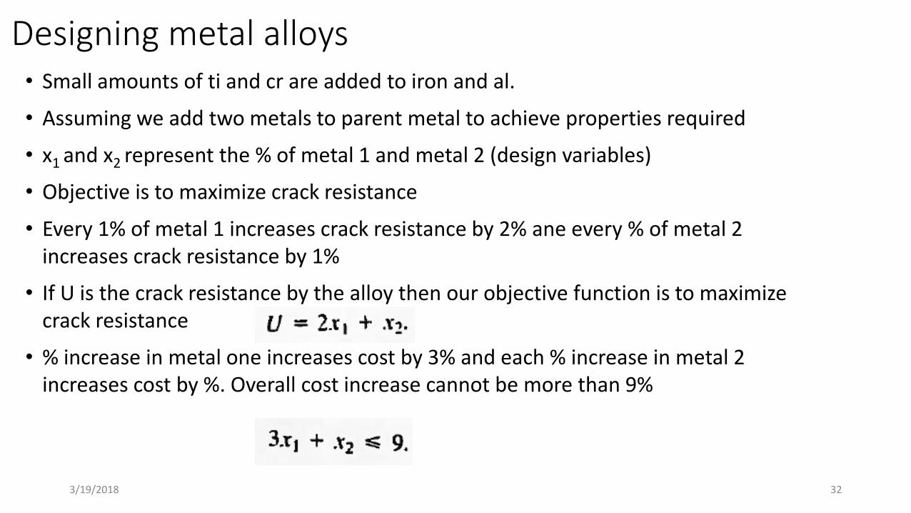
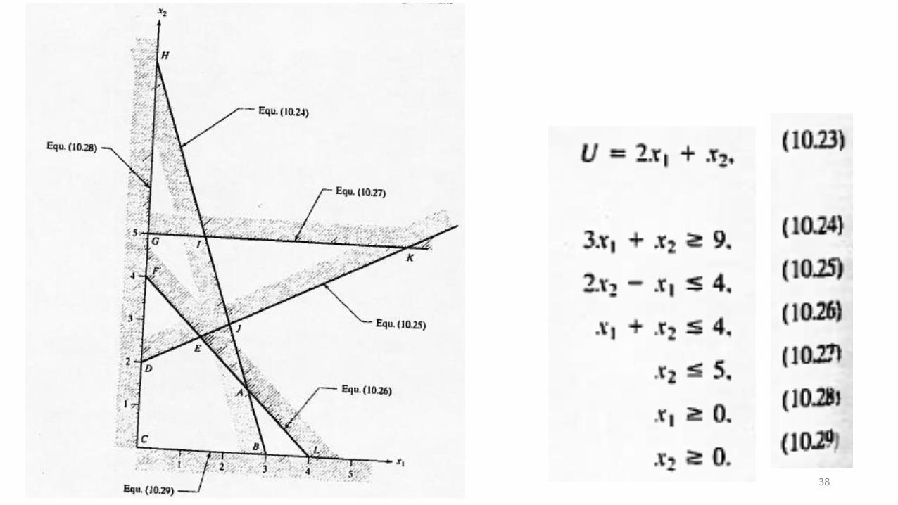
Designing metal alloys• Small amounts of ti and cr are added to iron and al.
• Assuming we add two metals to parent metal to achieve properties required
• x1 and x2 represent the % of metal 1 and metal 2 (design variables)
• Objective is to maximize crack resistance
• Every 1% of metal 1 increases crack resistance by 2% ane every % of metal 2 increases crack resistance by 1%
• If U is the crack resistance by the alloy then our objective function is to maximize crack resistance
• % increase in metal one increases cost by 3% and each % increase in metal 2 increases cost by %. Overall cost increase cannot be more than 9%

3/19/2018 33
Designing metal alloys• Metal 2 decreases corrosion resistance by 2% for every % and metal 1 increases
corrosion resistance 1% for every 1 %. Maximum acceptable decrease is 4%
• Melting temp - 1% of M1 decreases TM by 1% and 1% of M2 decreases TM by 1% total acceptable reduction is 4%
• Last constatint is there is only enough supply of M2 for 5% (due to demand)
• In addition the generic linear programming constraints also apply
• Geometrically these equations can be visualized as lines with inequality constraints marking the boundary (in the from of hatching)


• Rewriting the objective function as•
• Is an equation of line in the x1 x2 plane with a slope of -2
• And position of the line depends on the value of U
• If we take U = 0, then x1 and x2 have to be 0.
• As we increase the value of U, the number of potential x1 and x2 keeps increasing infinitely and it gets better with every increase
• The limiting value can be found from corner point A in the equation

3/19/2018 36
Simplex Algorithm• Simplex algorithm is the iterative process
• The geometric method of solving linear programming problems presented before. The graphical method is useful only for problems involving two decision variables and relatively few problem constraints.

3/19/2018 37
Minimizing the Objective function• Objective function, as in weight or cost, need to be minimized
• Use U’=-U and proceed to maximize U’ with simplex or graphical
• Reversal of constraint from less than to greater than
• Reworking the example that we did earlier with
• Reversing the direction of 10.8 as 10.24
3/19/2018 38

3/19/2018 39
• The new feasible region because of change in constraint is ABL and
• Similar to previous situation where U is 6.5, here the U is 8 which is the largest value

3/19/2018 40
Non Linear Programming• In linear programming, the optimum solution occurs at corner point
• So easier to identify optimum solution
• What do we do if either the objective function or the constranints are non linear
• You are trying to lay a 2 lane and 3 lane road with experienced and
inexperience ppl such that exp people does the 3 lane road at the same
time as inex does 2 lane
• Radio contact between the 2 teams is compulsory and it works only if
teams are less than 2 miles apart
• Objective function is U=3x1+2x2 (x1 and x2 are 3 and 2 lane road lengths
• The non linear constraint is x12+ x2
2=4 (equation of circle with radius 2)

3/19/2018 41
Non Linear Programming• Objective function is U=3x1+2x2 (x1 and x2 are 3 and 2 lane road lengths
• The non linear constraint is x12+ x2
2=4 (equation of circle with radius 2)
• The other 2 std equations are both x1 and x2 being > 0
• Feasible region is seen in the curve, with u = 6, and 8 shown, optimum
will be between these 2 Us, where the U-line is tangent to circle
• We can solve this using calculus based approach as well. We will see it
at the end

3/19/2018 42
Local and Global Optimum• Objective function is U=3x1+2x2 (x1 & x2 are 3 and 2 lane road
lengths
• In the modified problem if lengths are 5 and 3.5 miles and work plan
is start at extreme and work towards the intersection
• The radio receiver replaced with satellite phone, which requires the
distance to be more than 5 miles then the the non linear constraint
is (5-x1)2+ (3.5-x2)2>=25 (equation of circle with radius 5)
• The other 2 std equations are both x1 and x2 being > 0
• Feasible region is seen in the curve

3/19/2018 43
Local and Global Optimum• If you look at corner point A (x1 = 1.43 and x2 = 0), U = 4.3, and
moving in the direction of arrow, U reduces, giving a value of A as
optimum
• U in the neighborhood of A reduces so this is an optimum, until
when you go to point B ((x1 = 0 and x2 = 3.5) where U is 7
• Point B has the highest U and this is called the global optimum
• While Point A which has highest U in the nearby areas of A, is called
the local optimum
• If there is only one optimum as in previous problem (tangent) then
in that case both global and local are same
3/19/2018 44
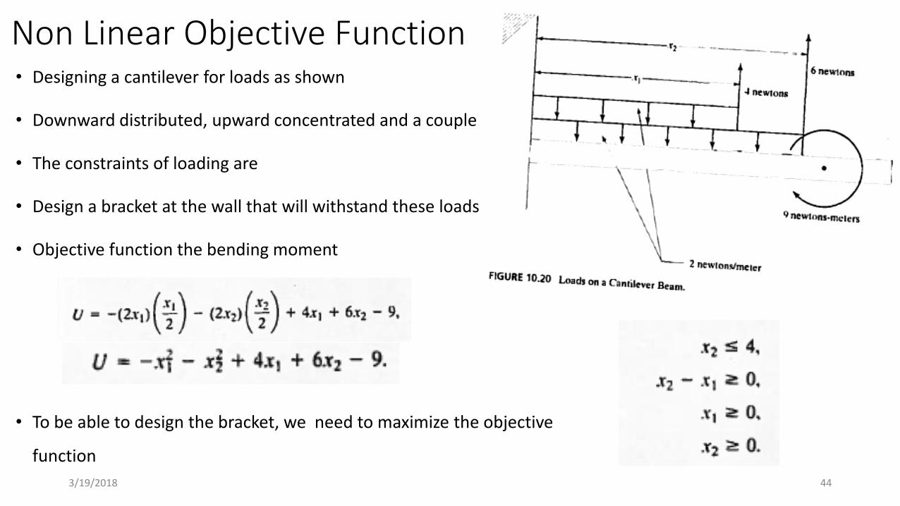
Non Linear Objective Function• Designing a cantilever for loads as shown
• Downward distributed, upward concentrated and a couple
• The constraints of loading are
• Design a bracket at the wall that will withstand these loads
• Objective function the bending moment
• To be able to design the bracket, we need to maximize the objective
function

3/19/2018 45
Non Linear Objective Function• Since u is nonlinear, curves are not straight lines
• It is a circle with center at x1 as 2 and x2 as 3
• Max U is 4, with radius 0. which like previous problems, is not in the
corner or at the end of the space (tangent)
• An efficient search strategy will be
• Select a starting point inside the possible domain or on the
boundary
• Find u, and increase values of x1 and x2 as by small margin and
identify U as such it is increasing and until the increase stops, which
will be the optimum value

3/19/2018 46
Non Linear Objective Function
• If a complex objective function is
• And the constraints associated with this function are below fig
• Feasible region and contour curves for U=0,4,8,12 are shown
• Two optima O1 and O2
• Depending on if we choose starting point as A or B, we will
converge to a different global optimum
• So for objective functions that have more than one optimum,
the optimum will depend on the choice of the starting point

3/19/2018 47
Optimum Design - Spring
• Minimizing the weight of coil spring, under tension
• Three design variables, coild dia ‘D’, wire dia ‘d’ and number of
turns ‘n’
• Objective function to be minimized is
• Using the equation for spring design, and substituting the
material properties for the spring, we can find 7 constraints for
the spring and then can minimize the objective function
3/19/2018 48
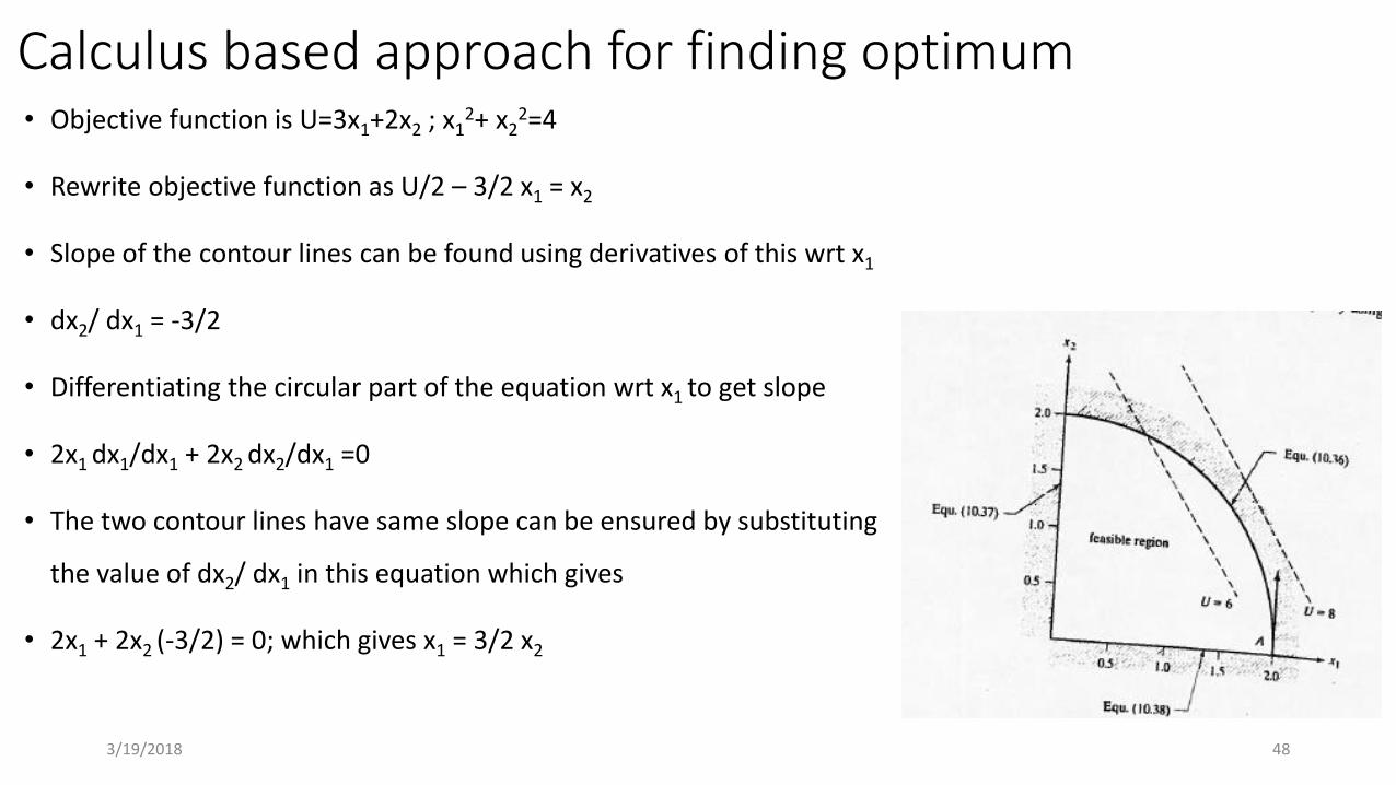
Calculus based approach for finding optimum• Objective function is U=3x1+2x2 ; x1
2+ x22=4
• Rewrite objective function as U/2 – 3/2 x1 = x2
• Slope of the contour lines can be found using derivatives of this wrt x1
• dx2/ dx1 = -3/2
• Differentiating the circular part of the equation wrt x1 to get slope
• 2x1 dx1/dx1 + 2x2 dx2/dx1 =0
• The two contour lines have same slope can be ensured by substituting
the value of dx2/ dx1 in this equation which gives
• 2x1 + 2x2 (-3/2) = 0; which gives x1 = 3/2 x2
3/19/2018 49
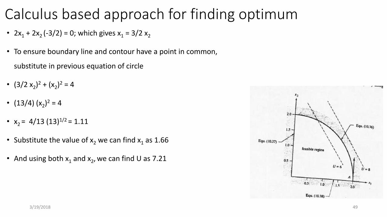
Calculus based approach for finding optimum• 2x1 + 2x2 (-3/2) = 0; which gives x1 = 3/2 x2
• To ensure boundary line and contour have a point in common,
substitute in previous equation of circle
• (3/2 x2)2 + (x2)2 = 4
• (13/4) (x2)2 = 4
• x2 = 4/13 (13)1/2 = 1.11
• Substitute the value of x2 we can find x1 as 1.66
• And using both x1 and x2, we can find U as 7.21