mechanical behavior of an aluminum alloy … behavior of an aluminum alloy and a structural steel...
TRANSCRIPT

MECHANICAL BEHAVIOR OF AN ALUMINUM ALLOY AND A STRUCTURAL STEEL UNDER MULTIAXIAL LOW CYCLE
FATIGUE
FREDERICO PORTÁSIO MIRANDA
DISSERTAÇÃO PARA OBTENÇÃO DE GRAU DE MESTRE EM
ENGENHARIA MECÂNICA
Júri
Presidente: Prof. Dr. Nuno Manuel Mendes Maia
Orientadores: Prof. Dr. Luis Filipe Galrão dos Reis
Prof. Dr. Bin Li
Vogal: Prof. Dr. Rui Fernando dos Santos Pereira Martins
SETEMBRO DE 2008

- ii -

- i -
Acknowledgements
I would like to thank the orientation of PhD Luis Reis. Without his guidance this dissertation
wouldn’t be possible. I also would like to thank sincerely to PhD Bin Li for the suggestions related to
the exploration of the different approaches to the problem, results analysis and work presentation.
People like Mr. Samões were very helpful in providing all the data and assistance necessary to
perform the preparation and properties tests of the materials.
Finally I also would like to thank to those who stood by me, my closest family and friends.

- ii -
- iii -
Abstract
Under service fatigue loading, cyclic plastic strain occurs and consequently fatigue cracks
nucleate, the mechanical resistance of the material will decrease. The simulation of the cyclic
stress/strain evolution and its distribution plays a fundamental role on fatigue life prediction of
mechanical components.
The objective of this dissertation is to study the Finite Element Method based algorithms for
improved fatigue life prediction under multiaxial loading conditions. Two distinct materials (a stainless
steel AISI 303 and an aluminium alloy 6060-T5) are studied and compared experimentally and
numerically under typical proportional and non-proportional loading paths.
Finite Element Code ABAQUS is applied to simulate the cyclic elastic-plastic stress/strain
behaviour; two element types (element type Pipe31 and C3D20R) are selected and compared. To
improve the simulation results, studies are also carried out on different mesh methods, different
hardening laws including the isotropic hardening, kinematic hardening, combined hardening, etc.
Based on the simulated local cyclic stress/strain results, various critical plane models are applied for
fatigue life prediction. By comparisons with experimental results, satisfactory agreements are shown
between the numerical simulations and experimental results.
Keywords: MUTIAXIAL FATIGUE;
LOADING PATHS;
PROPORTIONAL AND NON-PROPORTIONAL LOADINGS;
FATIGUE LIFE PREDICTION;
FINITE ELEMENT METHOD;
CRITICAL PLANES

- iv -
- v -
Resumo
Em carregamentos à fadiga em condições de serviço, é aplicada ao material deformação
plástica cíclica e consequentemente irá ocorrer nucleação de fendas assim como também a
dimininuição da resistência mecânica do material. A simulação da evolução tensão/deformação e a
sua distribuição desempenham um papel fundamental no cálculo da vida à fadiga de componentes
mecânicos.
O objectivo desta dissertação é de usar o método dos elementos finitos baseado em
algoritmos para calcular a vida à fadiga em diferentes condições de carregamento multiaxial. Para tal
efeito dois materiais distintos (Aço AISI 303 e uma liga de Alumínio 6060 com tratamento T5) são
estudados e comparados os valores obtidos experimentalmente e os obtidos numericamente sob
carregamentos típicos proporcionais e não proporcionais.
Usando o programa ABAQUS e seus elementos finitos é simulado o comportamento tensão
deformação elasto-plástico dos materiais, para este fim dois tipos de elementos (elementos Pipe31 e
C3D20R) foram escolhidos e comparados. Para melhorar os resultados das simulações, foram
aplicados diferentes malhas assim como diferentes leis de encruamento, incluíndo encruamento
isotrópico, cinemático e combinado, etc. Baseado nos resultados de simulações tensão/deformação
cíclicas locais foram aplicados métodos de plano crítico para calcular a vida à fadiga. São também
demonstradas algumas relações consideradas satisfatórias entre os valores experimentais e
numéricos.
Palavras Chave:
FADIGA MULITAXIAL;
TRAJECTÓRIAS DE CARREGAMENTO;
CARREGAMENTOS PROPORCIONAIS E NÃO PROPORCIONAIS;
PREDIÇÃO DE VIDA À FADIGA;
MÉTODO DOS ELEMENTOS FINITOS;
PLANOS CRÍTICOS

- vi -
- vii -
Index
Acknowledgements .............................................................................................................................. i
Abstract ............................................................................................................................................. iii
Keywords ........................................................................................................................................... iii
Resumo .............................................................................................................................................. v
Palavras Chave .................................................................................................................................. v
List of Figures .................................................................................................................................... ix
List of Tables ................................................................................................................................... xiii
List of Abbreviations .......................................................................................................................... xv
List of Symbols ................................................................................................................................. xv
1. Introduction .................................................................................................................................1
2. State of Art ..................................................................................................................................5
2.1. Proportional and Nonproportional Loading ......................................................................5
2.1.1. Estimating the Nonproportional Factor .......................................................................8
2.1.2. Additional Hardening ................................................................................................ 12
2.2. Low Cycle Fatigue Behaviour ....................................................................................... 13
2.2.1. Uniaxial and Biaxial .................................................................................................. 13
2.2.2. Isotropic and Kinematic Hardening ........................................................................... 15
2.2.3. Combined Hardening ............................................................................................... 18
2.2.3.1. Back Stress ......................................................................................................... 18
2.2.3.2. Flow formulation of Chaboche model ................................................................... 19
2.3. Biaxial Fatigue Life Prediction Theories ........................................................................ 23
2.3.1. Findley ..................................................................................................................... 23
2.3.2. Brown Miller Model .................................................................................................. 24
2.3.3. K.Liu Model .............................................................................................................. 26
2.3.4. Smith, Watson and Topper (S-W-T) Model ............................................................... 27
2.3.5. Fatemi and Socie (F-S) Model .................................................................................. 29
2.4. Additional research ...................................................................................................... 30
3. Experimental Procedure, Material and Equipment ...................................................................... 33
3.1. Introduction .................................................................................................................. 33
3.2. Materials ...................................................................................................................... 33
3.3. Specimens ................................................................................................................... 33
3.4. Equipment used ........................................................................................................... 34
3.5. Standards .................................................................................................................... 36
3.6. Strain Controlled Tests ................................................................................................. 36
3.6.1. Uniaxial Tensile Tests .............................................................................................. 36
3.6.2. The biaxial extensometer ......................................................................................... 37
4. Results and Analysis ................................................................................................................. 41
4.1. Introduction .................................................................................................................. 41
- viii -
4.2. Static Characterization of the Material .......................................................................... 41
4.2.1. Metallurgy analysis .................................................................................................. 41
4.2.2. Hardening tests ........................................................................................................ 42
4.2.3. Uniaxial tensile tests ................................................................................................ 42
4.3. Uniaxial and biaxial tests under controlled strain ........................................................... 43
5. Finite Element Method Study ..................................................................................................... 53
5.1. Introduction .................................................................................................................. 53
5.2. Building the Finite Element Models ............................................................................... 54
5.3. Choosing the Elements ................................................................................................ 54
5.3.1. C3D20R element ..................................................................................................... 54
5.3.2. Pipe31 element ........................................................................................................ 55
5.4. Definition and Mesh Dimension .................................................................................... 55
5.5. Boundary Conditions and Loads ................................................................................... 56
5.6. Hardening law .............................................................................................................. 58
5.7. Results......................................................................................................................... 58
5.7.1. Pipe31 elements strain paths ................................................................................... 59
5.7.2. Comparison between Pipe31 and C3D20R elements strain paths, eq. strain=0.60% 60
5.7.3. Pipe 31 Models AISI 303 .......................................................................................... 62
5.7.4. Pipe 31 Models Al6060–T5 0.60% ........................................................................... 71
5.8. Using Finite Elements to Predict Fatigue Life ................................................................ 72
5.8.1. Fatigue Life Prediction using Critical Plane Methods: AISI 303 ................................. 74
5.8.2. Fatigue Life Prediction using Critical Plane Methods: Al6060-T5............................... 75
5.9. Comments ................................................................................................................... 77
6. Conclusions ............................................................................................................................... 79
References ....................................................................................................................................... 81

- ix -
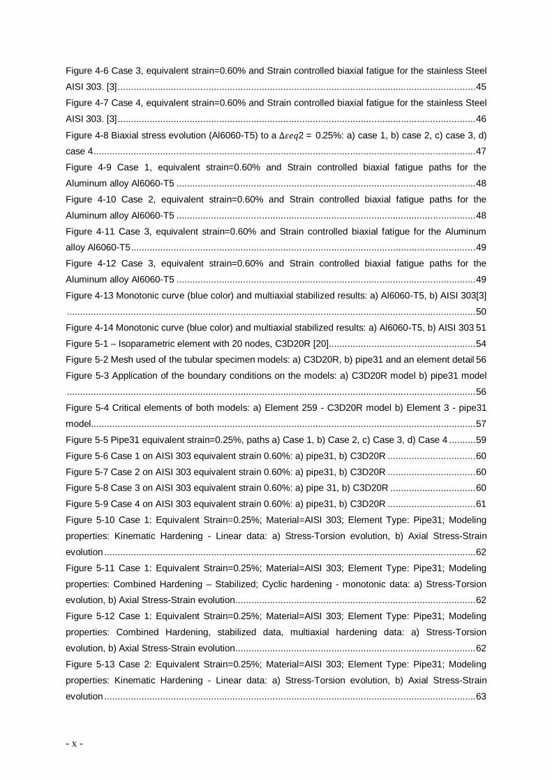
List of Figures Figure 2-1 Proportional biaxial loading of a shaft [3,4]..........................................................................5
Figure 2-2 Nonproportional tension-torsion load [3,4] ..........................................................................6
Figure 2-3 Proportional biaxial loading: a) in phase with mean strain; b) Out-of-Phase [3,4] .................7
Figure 2-4 Proportional loading of a drum pulley shaft [3,4] .................................................................7
Figure 2-5 Proportional (0 and 5) and nonproportional (1-4 and 6-13) loading histories [3,4] ................8
Figure 2-6 Nonproportional loading histories, a) different phases, b) different amplitude [3,4] ..............9
Figure 2-7 Crossed Hardening effect [3] ............................................................................................ 11
Figure 2-8 Possible material behavior to monotonic curves and steady cycles [3] .............................. 15
Figure 2-9 The Bauschinger effect [3] ................................................................................................ 16
Figure 2-10 Isotropic hardening [3,4] ................................................................................................. 16
Figure 2-11 Kinematic hardening model [3,4] .................................................................................... 17
Figure 2-12 Isotropic and kinematic hardening during nonproportional cyclic loading ......................... 17
Figure 2-13. a) smooth transient, b) non smooth transient [6] ............................................................ 20
Figure 2-14 Ratcheting [3,4] .............................................................................................................. 22
Figure 2-15 Nonproportional biaxial loading for a shaft [3,4] .............................................................. 22
Figure 2-16 Crack type A and B [3].................................................................................................... 25
Figure 2-17 Strain energy: Elastic and plastic [3] ............................................................................... 26
Figure 2-18 The S-W-T physical basis [3,4] ....................................................................................... 28
Figure 2-19 Fatemi-Socie physics model [3,4] .................................................................................. 29
Figure 3-1 AISI 303 geometry and dimensions of the tubular specimens according to the standard
ASTM E2207 [17].............................................................................................................................. 34
Figure 3-2 Al6060-T5 geometry and dimensions of the tubular specimens according to the standard
ASTM E2207 [17].............................................................................................................................. 34
Figure 3-3 Servo Hydraulic scheme [3] .............................................................................................. 35
Figure 3-4 Servo hydraulic device, model Instron 8874 ...................................................................... 36
Figure 3-5 Uniaxial extensometer brand: Instron CAT Nº 2620-602 [3] .............................................. 37
Figure 3-6 Extensometer axial/torsional model 3550 used on the biaxial tests ................................... 37
Figure 3-8 Strain controlled biaxial fatigue paths: a) Case 1; b) Case 2; c) Case 3; d) Case 4 ........... 39
Figure 3-9 Strain controlled biaxial fatigue strains: a) Case 1; b) Case 2; c) Case 3; d) Case 4 .......... 39
Figure 4-1 AISI 303 microstructure, attacked with ethanedioic acid. Amplification: a) 200x, b) 1000x [3]
......................................................................................................................................................... 41
Figure 4-2 Al6060-T5 microstructure, attacked with Keller. Amplified: a) 200x, b) 400x ...................... 42
Figure 4-3 Biaxial stress evolution (AISI303) to a ∆휀푒푞2 = 0.25%: a) case 1, b) case 2, c) case 3, d)
case 4. [3] ......................................................................................................................................... 44
Figure 4-4 Case 1, equivalent strain=0.60% and Strain controlled biaxial fatigue paths for the stainless
Steel AISI 303. [3] ............................................................................................................................. 44
Figure 4-5 Case 2, equivalent strain=0.60% and Strain controlled biaxial fatigue for the stainless Steel
AISI 303. [3] ...................................................................................................................................... 45
- x -
Figure 4-6 Case 3, equivalent strain=0.60% and Strain controlled biaxial fatigue for the stainless Steel
AISI 303. [3] ...................................................................................................................................... 45
Figure 4-7 Case 4, equivalent strain=0.60% and Strain controlled biaxial fatigue for the stainless Steel
AISI 303. [3] ...................................................................................................................................... 46
Figure 4-8 Biaxial stress evolution (Al6060-T5) to a ∆휀푒푞2 = 0.25%: a) case 1, b) case 2, c) case 3, d)
case 4 ............................................................................................................................................... 47
Figure 4-9 Case 1, equivalent strain=0.60% and Strain controlled biaxial fatigue paths for the
Aluminum alloy Al6060-T5 ................................................................................................................ 48
Figure 4-10 Case 2, equivalent strain=0.60% and Strain controlled biaxial fatigue paths for the
Aluminum alloy Al6060-T5 ................................................................................................................ 48
Figure 4-11 Case 3, equivalent strain=0.60% and Strain controlled biaxial fatigue for the Aluminum
alloy Al6060-T5 ................................................................................................................................. 49
Figure 4-12 Case 3, equivalent strain=0.60% and Strain controlled biaxial fatigue paths for the
Aluminum alloy Al6060-T5 ................................................................................................................ 49
Figure 4-13 Monotonic curve (blue color) and multiaxial stabilized results: a) Al6060-T5, b) AISI 303[3]
......................................................................................................................................................... 50
Figure 4-14 Monotonic curve (blue color) and multiaxial stabilized results: a) Al6060-T5, b) AISI 303 51
Figure 5-1 – Isoparametric element with 20 nodes, C3D20R [20] ....................................................... 54
Figure 5-2 Mesh used of the tubular specimen models: a) C3D20R, b) pipe31 and an element detail 56
Figure 5-3 Application of the boundary conditions on the models: a) C3D20R model b) pipe31 model
......................................................................................................................................................... 56
Figure 5-4 Critical elements of both models: a) Element 259 - C3D20R model b) Element 3 - pipe31
model................................................................................................................................................ 57
Figure 5-5 Pipe31 equivalent strain=0.25%, paths a) Case 1, b) Case 2, c) Case 3, d) Case 4 .......... 59
Figure 5-6 Case 1 on AISI 303 equivalent strain 0.60%: a) pipe31, b) C3D20R ................................. 60
Figure 5-7 Case 2 on AISI 303 equivalent strain 0.60%: a) pipe31, b) C3D20R ................................. 60
Figure 5-8 Case 3 on AISI 303 equivalent strain 0.60%: a) pipe 31, b) C3D20R ................................ 60
Figure 5-9 Case 4 on AISI 303 equivalent strain 0.60%: a) pipe31, b) C3D20R ................................. 61
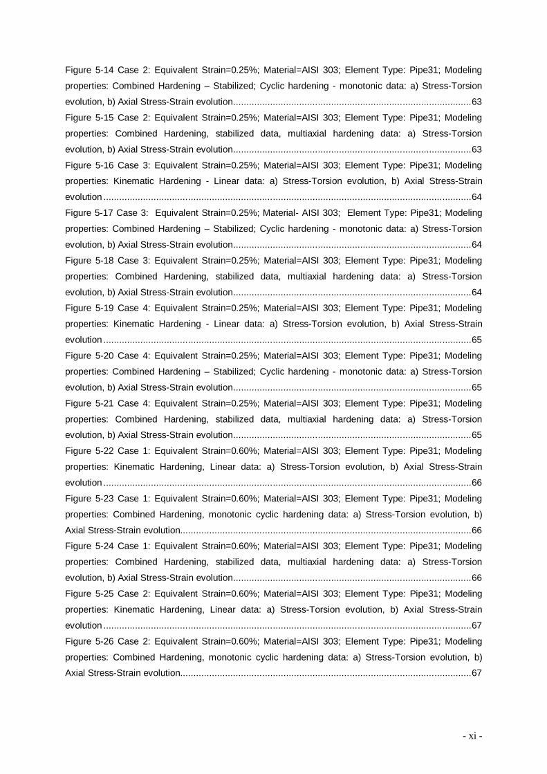
Figure 5-10 Case 1: Equivalent Strain=0.25%; Material=AISI 303; Element Type: Pipe31; Modeling
properties: Kinematic Hardening - Linear data: a) Stress-Torsion evolution, b) Axial Stress-Strain
evolution ........................................................................................................................................... 62
Figure 5-11 Case 1: Equivalent Strain=0.25%; Material=AISI 303; Element Type: Pipe31; Modeling
properties: Combined Hardening – Stabilized; Cyclic hardening - monotonic data: a) Stress-Torsion
evolution, b) Axial Stress-Strain evolution .......................................................................................... 62
Figure 5-12 Case 1: Equivalent Strain=0.25%; Material=AISI 303; Element Type: Pipe31; Modeling
properties: Combined Hardening, stabilized data, multiaxial hardening data: a) Stress-Torsion
evolution, b) Axial Stress-Strain evolution .......................................................................................... 62
Figure 5-13 Case 2: Equivalent Strain=0.25%; Material=AISI 303; Element Type: Pipe31; Modeling
properties: Kinematic Hardening - Linear data: a) Stress-Torsion evolution, b) Axial Stress-Strain
evolution ........................................................................................................................................... 63
- xi -
Figure 5-14 Case 2: Equivalent Strain=0.25%; Material=AISI 303; Element Type: Pipe31; Modeling
properties: Combined Hardening – Stabilized; Cyclic hardening - monotonic data: a) Stress-Torsion
evolution, b) Axial Stress-Strain evolution .......................................................................................... 63
Figure 5-15 Case 2: Equivalent Strain=0.25%; Material=AISI 303; Element Type: Pipe31; Modeling
properties: Combined Hardening, stabilized data, multiaxial hardening data: a) Stress-Torsion
evolution, b) Axial Stress-Strain evolution .......................................................................................... 63
Figure 5-16 Case 3: Equivalent Strain=0.25%; Material=AISI 303; Element Type: Pipe31; Modeling
properties: Kinematic Hardening - Linear data: a) Stress-Torsion evolution, b) Axial Stress-Strain
evolution ........................................................................................................................................... 64
Figure 5-17 Case 3: Equivalent Strain=0.25%; Material- AISI 303; Element Type: Pipe31; Modeling
properties: Combined Hardening – Stabilized; Cyclic hardening - monotonic data: a) Stress-Torsion
evolution, b) Axial Stress-Strain evolution .......................................................................................... 64
Figure 5-18 Case 3: Equivalent Strain=0.25%; Material=AISI 303; Element Type: Pipe31; Modeling
properties: Combined Hardening, stabilized data, multiaxial hardening data: a) Stress-Torsion
evolution, b) Axial Stress-Strain evolution .......................................................................................... 64
Figure 5-19 Case 4: Equivalent Strain=0.25%; Material=AISI 303; Element Type: Pipe31; Modeling
properties: Kinematic Hardening - Linear data: a) Stress-Torsion evolution, b) Axial Stress-Strain
evolution ........................................................................................................................................... 65
Figure 5-20 Case 4: Equivalent Strain=0.25%; Material=AISI 303; Element Type: Pipe31; Modeling
properties: Combined Hardening – Stabilized; Cyclic hardening - monotonic data: a) Stress-Torsion
evolution, b) Axial Stress-Strain evolution .......................................................................................... 65
Figure 5-21 Case 4: Equivalent Strain=0.25%; Material=AISI 303; Element Type: Pipe31; Modeling
properties: Combined Hardening, stabilized data, multiaxial hardening data: a) Stress-Torsion
evolution, b) Axial Stress-Strain evolution .......................................................................................... 65
Figure 5-22 Case 1: Equivalent Strain=0.60%; Material=AISI 303; Element Type: Pipe31; Modeling
properties: Kinematic Hardening, Linear data: a) Stress-Torsion evolution, b) Axial Stress-Strain
evolution ........................................................................................................................................... 66
Figure 5-23 Case 1: Equivalent Strain=0.60%; Material=AISI 303; Element Type: Pipe31; Modeling
properties: Combined Hardening, monotonic cyclic hardening data: a) Stress-Torsion evolution, b)
Axial Stress-Strain evolution.............................................................................................................. 66
Figure 5-24 Case 1: Equivalent Strain=0.60%; Material=AISI 303; Element Type: Pipe31; Modeling
properties: Combined Hardening, stabilized data, multiaxial hardening data: a) Stress-Torsion
evolution, b) Axial Stress-Strain evolution .......................................................................................... 66
Figure 5-25 Case 2: Equivalent Strain=0.60%; Material=AISI 303; Element Type: Pipe31; Modeling
properties: Kinematic Hardening, Linear data: a) Stress-Torsion evolution, b) Axial Stress-Strain
evolution ........................................................................................................................................... 67
Figure 5-26 Case 2: Equivalent Strain=0.60%; Material=AISI 303; Element Type: Pipe31; Modeling
properties: Combined Hardening, monotonic cyclic hardening data: a) Stress-Torsion evolution, b)
Axial Stress-Strain evolution.............................................................................................................. 67

- xii -
Figure 5-27 Case 2: Equivalent Strain=0.60%; Material=AISI 303; Element Type: Pipe31; Modeling
properties: Combined Hardening, stabilized data, multiaxial hardening data: a) Stress-Torsion
evolution, b) Axial Stress-Strain evolution .......................................................................................... 67
Figure 5-28 Case 3: Equivalent Strain=0.60%; Material=AISI 303; Element Type: Pipe31; Modeling
properties: Kinematic Hardening, Linear data: a) Stress-Torsion evolution, b) Axial Stress-Strain
evolution ........................................................................................................................................... 68
Figure 5-29 Case 3: Equivalent Strain=0.60%; Material=AISI 303; Element Type: Pipe31; Modeling
properties: Combined Hardening, monotonic cyclic hardening data: a) Stress-Torsion evolution, b)
Axial Stress-Strain evolution.............................................................................................................. 68
Figure 5-30 Case 3: Equivalent Strain=0.60%; Material=AISI 303; Element Type: Pipe31; Modeling
properties: Combined Hardening, stabilized data, multiaxial hardening data: a) Stress-Torsion
evolution, b) Axial Stress-Strain evolution .......................................................................................... 68
Figure 5-31 Case 4: Equivalent Strain=0.60%; Material=AISI 303; Element Type: Pipe31; Modeling
properties: Kinematic Hardening, Linear data: a) Stress-Torsion evolution, b) Axial Stress-Strain
evolution ........................................................................................................................................... 69
Figure 5-32 Case 4: Equivalent Strain=0.60%; Material=AISI 303; Element Type: Pipe31; Modeling
properties: Combined Hardening, monotonic cyclic hardening data: a) Stress-Torsion evolution, b)
Axial Stress-Strain evolution.............................................................................................................. 69
Figure 5-33 Case 4: Equivalent Strain=0.60%; Material=AISI 303; Element Type: Pipe31; Modeling
properties: Combined Hardening, stabilized data, multiaxial hardening data: a) Stress-Torsion
evolution, b) Axial Stress-Strain evolution .......................................................................................... 69
Figure 5-34 Case 1: Equivalent Strain=0.60%; Material=Al6060-T5; Element Type: Pipe31; Modeling
properties: Combined Hardening – Stabilized; Cyclic hardening - monotonic data a) Stress-Torsion
evolution, b) Axial Stress-Strain evolution .......................................................................................... 71
Figure 5-35 Case 2: Equivalent Strain=0.60%; Material=Al6060-T5; Element Type: Pipe31; Modeling
properties: Combined Hardening – Stabilized; Cyclic hardening - monotonic data: a) Stress-Torsion
evolution, b) Axial Stress-Strain evolution .......................................................................................... 71
Figure 5-36 Case 3: Equivalent Strain=0.60%; Material=Al6060-T5; Element Type: Pipe31; Modeling
properties: : Combined Hardening, monotonic cyclic hardening data: a) Stress-Torsion evolution, b)
Axial Stress-Strain evolution.............................................................................................................. 71
Figure 5-37 Case 4: Equivalent Strain=0.60%; Material=Al6060-T5; Element Type: Pipe31; Modeling
properties: Combined Hardening – Stabilized; Cyclic hardening - monotonic data a) Stress-Torsion
evolution, b) Axial Stress-Strain evolution .......................................................................................... 72
- xiii -
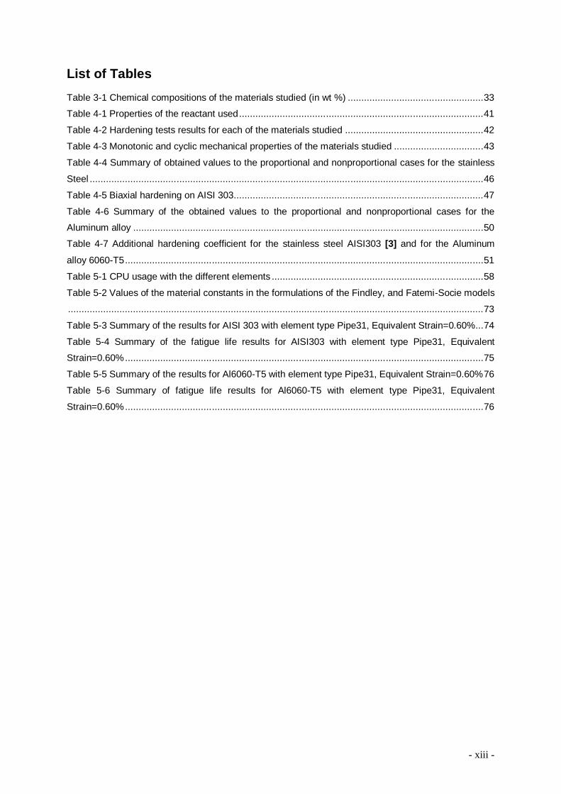
List of Tables Table 3-1 Chemical compositions of the materials studied (in wt %) .................................................. 33
Table 4-1 Properties of the reactant used .......................................................................................... 41
Table 4-2 Hardening tests results for each of the materials studied ................................................... 42
Table 4-3 Monotonic and cyclic mechanical properties of the materials studied ................................. 43
Table 4-4 Summary of obtained values to the proportional and nonproportional cases for the stainless
Steel ................................................................................................................................................. 46
Table 4-5 Biaxial hardening on AISI 303 ............................................................................................ 47
Table 4-6 Summary of the obtained values to the proportional and nonproportional cases for the
Aluminum alloy ................................................................................................................................. 50
Table 4-7 Additional hardening coefficient for the stainless steel AISI303 [3] and for the Aluminum
alloy 6060-T5 .................................................................................................................................... 51
Table 5-1 CPU usage with the different elements .............................................................................. 58
Table 5-2 Values of the material constants in the formulations of the Findley, and Fatemi-Socie models
......................................................................................................................................................... 73
Table 5-3 Summary of the results for AISI 303 with element type Pipe31, Equivalent Strain=0.60%... 74
Table 5-4 Summary of the fatigue life results for AISI303 with element type Pipe31, Equivalent
Strain=0.60% .................................................................................................................................... 75
Table 5-5 Summary of the results for Al6060-T5 with element type Pipe31, Equivalent Strain=0.60% 76
Table 5-6 Summary of fatigue life results for Al6060-T5 with element type Pipe31, Equivalent
Strain=0.60% .................................................................................................................................... 76

- xiv -

- xv -
List of Abbreviations AISI “American Iron and Steel Institute”
ASTM “American Society for Testing and Materials”
B-M “Brown-Miller”
b.c.c. body centered cubic f.c.c. face centered cubic
CPA Critical Plane Approach
F.E.M Finite Element Method
F-S Fatemi-Socie
H.C.F. High Cycle Fatigue
HV Vickers Hardening
IST Instituto Superior Técnico
LCF Low Cycle Fatigue
NP Nonproporcional
S-W-T Smith-Watson-Topper
List of Symbols am Mean crack length
a half length surface crack
An Effective strain of a material
b Fatigue strength exponent
bγ Shear fatigue strength exponent
c fatigue ductility exponent
cγ Torsion fatigue ductility exponent
C Paris coeficient
da/dN Crack propagation velocity
E Elasticity modulus
FNP Nonproportional factor
f-1 fatigue stress limit under alternated flection (R=-1)
fo fatigue stress limit under repited flection (R=0)
G Shear elasticity modulus
K Strength coefficient
K’ Cyclic strength coefficient
kt Elastic stress concentration factor
kf Fatigue strength reduction factor
m Paris law exponent
n Strain hardening exponent
n’ Cyclic strain hardening exponent

- xvi -
N Number of cycles
Nf Number of cycles at the time of rupture
2Nf Reversions until rupture
2NT Reversions at the time of transition between LCF and HCF regime
PH Hydrostatic pressure
ry Plastic zone dimension
S-1 Stress fatigue limit under tensile stress-compression (R=-1)
S0 Stress limit under tensile stress-compression fatigue (R=0)
t Time
t-1 Stress fatigue limit Tensão under alternating torsion (R=-1)
T Period
휔 Frequency
W Energy
ε Normal strain
εn Plane normal strain
εxo Initial normal strain
εx , εy , εz Normal strains coordinate system x-y-z
ε1 , ε2 , ε3 Principal normal strains
εθ Normal strain on a plane θ
εeq. Equivalent strain εnom. Nominal strain
Δε Normal strain amplitude
Δε1 , Δε2 , Δε3 Principal normal strain amplitude
Δεx , Δεy , Δεz Principal normal strain amplitude coordinate system x-y-z
Δεe Elastic strain amplitude
Δεn Normal strain amplitude
ΔεNP Non proportional strain/strain amplitude
Δεp Plastic strain/strain amplitude
휀 Fatigue ductility coeficient
γ Distortion/shear strain
γxy, γyz, γxz, Distortion coordinate system x-y-z
Δγxy, Δγyz, Δγxz, Distortion amplitude coordinate system x-y-z
γxyo Initial distortion
γ13, γ23, γ12, Principal distortion
γθ Distortion on a θ plane
Δγ Distortion amplitude
γf’ Shear fatigue ductility coefficient
ν Poisson’s ratio
σ, Δσ Stress, (amplitude)
σa Normal stress amplitude

- xvii -
σa, R=-1 Alternated fatigue stress limit Tension-compression (R=-1)
σa, R=0 Alternated fatigue stress limit Tension-compression (R=0)
σa, R=0.5 Corrugated fatigue stress limit tension-compression (R=0.5)
σy Yield stress
σeq, Δσeq Equivalent stress, (amplitude)
σh Hydrostatic stress
σH,av Average hydrostatic stress
σH,max Tensão hidrostática máxima
휎 Fatigue strength coefficient
σmax Maximum normal stress
σm Mean normal stress
σmin Minimum normal stress
σnom Nominal stress
σNP von Mises Non proportional equivalent stress σP Equivalent proportional Von Mises stress
σr Rupture stress
σx , σy , σz Normal stresses coordinate system x-y-z
σx,med, σy,med, σz,med Normal mean stresses coordinate system x-y-z
σxo Initial normal stress
σy Yield stress
σ1 , σ2 , σ3 Principal normal stresses
휏, Δ휏 Shear stress (amplitude)
휏 Shear stress amplitude
휏 Mean shear stress
휏 , 휏 , 휏 Shear stress coordinate system x-y-z
휏 , 휏 , 휏 Principal shear stress
휏 Shear fatigue ductlility exponent

- xviii -

- 1 -
1. Introduction Age hardened Aluminium alloys are of great technological importance, in particular for ground
transport systems. When relatively high strength, good corrosion resistance and high toughness are
required in conjunction with good formability and weldability, aluminium alloys with Mg and Si as
alloying elements (Al–Mg–Si, 6xxx Aluminium series alloys) are used. The comparison of experimental
and theoretical results under biaxial fatigue between high strength steels and aluminium alloys has an
important role to choose which material would be better to a certain end. [1]
The investigation of early crack growth due to multiaxial fatigue is one branch of the wide field
of research in multiaxial fatigue since most of fatigue accidents occur due to this kind of loads.
Several methods to predict multiaxial fatigue loads have been developed in the last forty years
and mainly due to change of directions and ratio variations of the principal stresses, classic
approaches are not always conservative under multiaxial loads. As a result in the last decades,
several multiaxial fatigue criteria based on critical plane and also on integral, invariant and energy
approaches have been proposed. However the existing multiaxial fatigue models were developed to
specific load conditions and the application to more general projects require more study. A few
examples of applicable and promising critical plane methods on low cycle multiaxial fatigue are the
Brown-Miller and Fatemi-Socie methods which are able to determinate the damage plane strain and
stress levels. [2-3]
The ABAQUS program is used to evaluate the numerical results of the cyclic stress and strain
evolution under proportional and nonproportional biaxial loading.
The cyclic elasto-plastic response and local deformations are analyzed using the F.E.M.
program ABAQUS, with two main objectives, complementing the experimental results of the cyclic
behaviour under certain loading situation of the material, and in other way to use the F.E. potential to
determine when stress and strain values stabilize in a way to include those values in predicting models
under multiaxial fatigue.
In this research an Aluminium alloy is tested, and so, the life of the components can be
predicted/estimated using multiaxial fatigue criteria. A usual procedure on fatigue design is to initiate
the study with the calculations of the local elastic stress-time history so critical zones can be detected
on a component or structure, using the finite element method. Next an evaluation on a critical zone is
carried out under a certain number of cyclic loads, and the existence of cracks can be evaluated by
the application of an appropriated multiaxial fatigue criterion. [3]
Multiaxial stress states can occur either due to multiaxial loading or to local induced multiaxial
stress states (on notches, on contact points, etc.) or due to residual stress states due to machining,
etc. In engineering design, conventional approaches based on uniaxial fatigue data may estimate
nonconservative lives for complex multiaxial fatigue loading. For a safe and reliable design of
- 2 -
components, it is needed to study the effects of multiaxial loading and particularly the non-proportional
loadings on the fatigue damage.
The objective of this work is to evaluate the mechanical behavior, in particular the proportional
and non-proportional fatigue parameters, on 6060-T5 aluminum alloy and their comparison with similar
results obtained for stainless steels AISI 303, suitable for estimating non-proportional low cycle fatigue
lives. Since the stabilized cyclic stress/strain fields are essential for fatigue life predictions, local
elasto-plastic behavior of the material are studied first. The additional hardening coefficient, (), based
on the stabilized cyclic stress/strain cycle is evaluated for correlating the fatigue lives obtained in the
tests.
Materials may have very different additional hardening behavior, under multiaxial cyclic
loading paths. Depending on the loading amplitude and loading level, stress relaxations occur and the
stabilized cyclic stress/strain state may be very different from the initial one. Elasto-plastic FEM
analysis, using ABAQUS Code, were carried out in order to predict the stabilized cyclic stress/strain
state, under the same multiaxial loading paths used on the experimental tests. Two models were used;
a linear beam element pipe31 with 4 integration points and an Isoparametric solid element with 20
nodes were used on the mesh modeling.
Results show that metallic materials present different behavior concerning additional
hardening which is of prime importance for predicting fatigue life.
A short introduction to each chapter:
The chapter II includes the state of the art of multiaxial fatigue. In this chapter it will be
introduced the most relevant aspects of the field of study: strain controlled low cycle biaxial fatigue.
The chapter III is dedicated to the materials tested, the equipment and the experimental
procedure. Here are described the materials and they’re main characteristics, the equipment needed,
its capacities and characteristics, the standards used as reference to the experimental procedures,
and in the last part of the chapter is also described the methodology used on the strain controlled
biaxial fatigue tests.
The chapter IV includes the results and the analysis of all experimental study. The
methodology used was the following one: the results for each of the subjects and the 2 materials tests
are presented and right after they are analyzed. Results are presented under the form of graphics
tables and images.
The chapter V is the Numerical Study. Considered the main chapter, where are presented the
different models for each of the different elements used to model the specimens, and it is also

- 3 -
presented the mesh definition, the number of nodes and elements needed for each specimen,
boundary conditions and loads for all the different cases. It is also described the procedure of the
Finite Elements contribution to predict the fatigue life and the different application fields to each of the
numerical simulations. Like in the previous chapter it is also presented.
The chapter VI presents the conclusions and proposals for further developments. This chapter
closes this dissertation with the most relevant conclusions to all the work done, if exists or not
consistence between the proposed objective and the reached results. In the second part of this
chapter it is presented a few possibilities to further development, such as uncertainties which were not
fully developed and also leads to new areas.

- 4 -
- 5 -
2. State of Art
2.1. Proportional and Nonproportional Loading
In the presence of a cyclic load the orientation of the principal axis can change in relation with
the component or magnitude, the principal stresses can also change with the time. In general cases
both magnitude and orientation change with time.
Multiaxial fatigue life can be easily influenced if principal axis changes with time, and when
observed extra care must be employed when extrapolating uniaxial fatigue theories to more general
loading cases. [3]
Proportionality and additional hardening are two common terms in multiaxial fatigue that
increase the hardening of the materials: Proportional loading cases increase the hardening of the
material by fatigue damage mechanisms and the additional hardening is related with alteration of the
dislocation substructure caused by the cyclic plastic strain along multiple slip mechanisms of the
material structure.
Nonproportional load can be defined mechanically in terms of the rotation of the principal
strain planes. From the fatigue viewpoint a strain path that results in a fixed orientation of the principal
axis associated with the alternation of strain components is proportional to the strain history and is
nonproportional if the principal axis rotates with time. In both cases only the alternate or cyclic strains
are taken in consideration because static strains do not influence the reverse shear direction. [3,4]
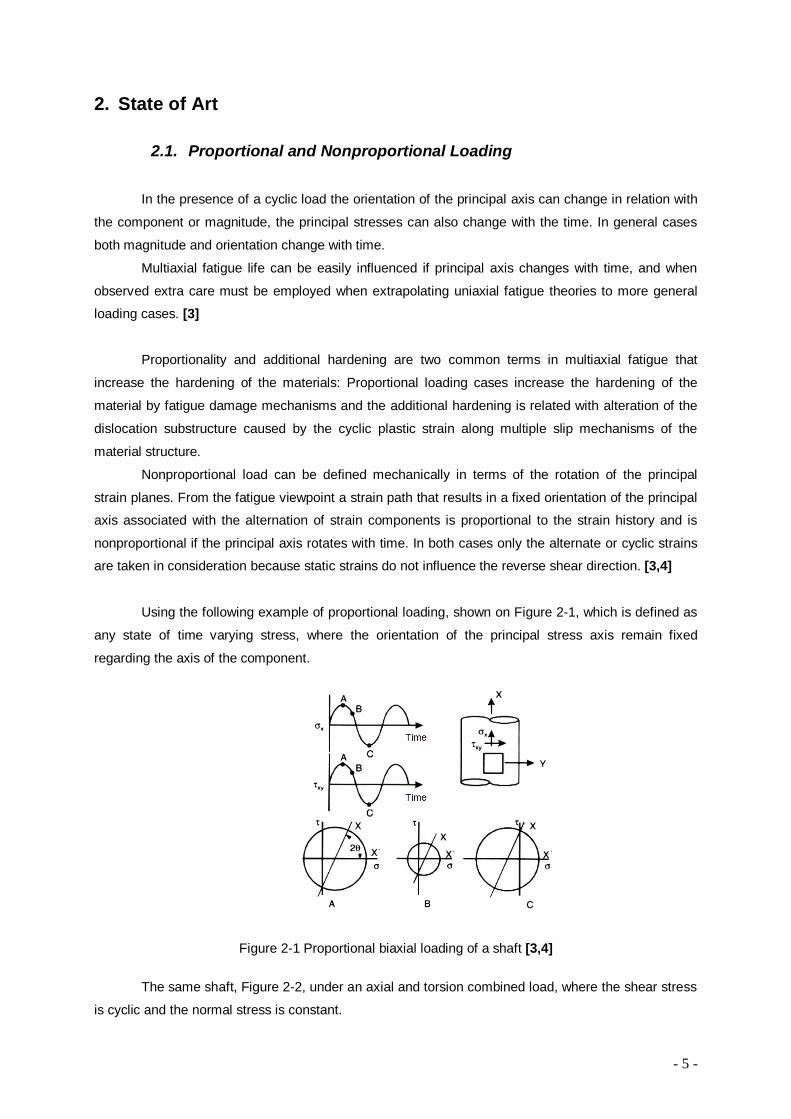
Using the following example of proportional loading, shown on Figure 2-1, which is defined as
any state of time varying stress, where the orientation of the principal stress axis remain fixed
regarding the axis of the component.
Figure 2-1 Proportional biaxial loading of a shaft [3,4]
The same shaft, Figure 2-2, under an axial and torsion combined load, where the shear stress
is cyclic and the normal stress is constant.

- 6 -
Figure 2-2 Nonproportional tension-torsion load [3,4]
In this case it can be observed that the shear stress varies with time and normal stress is
always constant. From the load analysis of the load in points A, B, C, D and E the associated Mohr
circle changes with the dimension and the reference X’ associated with the principal stress (A), not
always matches with the principal stress. In this case we have a nonproportional load, i.e. at any
moment of the load history the orientation of the principal stress axis varies relatively to the
components axis. If the Von Mises effective stress is calculated from the Figure 2-2, this stress will be
constant at every moment, which means that the octahedral effective stress is not sensitive to the
variations of the stress cyclic components, and concluding that it can’t estimate the damage
occurrence in nonproportional situations. [3,4]
Out-of-phase and in-phase are terms to describe special loading cases which involve periodic
histories such as sine or triangular waveforms. Tension-torsion out-of-phase loadings will always be
nonproportional and in-phase loading will always be proportional. Materials subject to 90º out-of-phase
exhibit the greatest degree of additional nonproportional cyclic hardening.
Therefore under an in-phase or out-of-phase load history, where both paths provide the same
principal shear strain magnitude, the out-of-phase load history will always produce equal or greater
damage. The amount of damage increased depends on the sensitivity of the material to normal
stresses and strains.
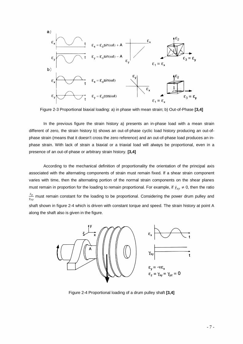
The loading history in Figure 2-3 shows that the rotation of the principal strain axis is found
only in out-of-phase normal and shear strains. Out-of-phase normal strains do not produce rotation of
the principal strains.
- 7 -
Figure 2-3 Proportional biaxial loading: a) in phase with mean strain; b) Out-of-Phase [3,4]
In the previous figure the strain history a) presents an in-phase load with a mean strain
different of zero, the strain history b) shows an out-of-phase cyclic load history producing an out-of-
phase strain (means that it doesn’t cross the zero reference) and an out-of-phase load produces an in-
phase strain. With lack of strain a biaxial or a triaxial load will always be proportional, even in a
presence of an out-of-phase or arbitrary strain history. [3,4]
According to the mechanical definition of proportionality the orientation of the principal axis
associated with the alternating components of strain must remain fixed. If a shear strain component
varies with time, then the alternating portion of the normal strain components on the shear planes
must remain in proportion for the loading to remain proportional. For example, if 훾 ≠ 0, then the ratio
must remain constant for the loading to be proportional. Considering the power drum pulley and
shaft shown in figure 2-4 which is driven with constant torque and speed. The strain history at point A
along the shaft also is given in the figure.
Figure 2-4 Proportional loading of a drum pulley shaft [3,4]

- 8 -
According to the mechanical definition of a proportional loading, the orientation of the principal
axis must remain fixed. In this case only the normal components 휀 and 휀 varies through time, but
since they are proportional, the loading is also proportional and so the additional cyclic hardening will
not be present. [3,4]
Proportional and nonproportional loads can be easily visualized by drawing the strain space
history, with normal strains vs. each of the two shear strains on the same plane. The results of these
combinations are: 휀 vs. , 휀 vs. , 휀 vs. , 휀 vs. , 휀 vs. , 휀 vs. . (Note: if the plots
show either a straight line or a single point, the history will be proportional).
The Figure 2-5 shows the a few cases of proportional and non proportional loading cases.
Figure 2-5 Proportional (0 and 5) and nonproportional (1-4 and 6-13) loading histories [3,4]
The nonproportional loading histories can create some issues, some of them being: a) the
additional hardening in some materials. This issue must be taken in account during analysis of a
plasticity cycle and should be included on the damage parameter in the form of the stress amplitude,
maximum stress and energy, b) counting the cycles. In a uniaxial load, the “Rain Flow” is well defined
and generally accepted to define each cycle along a complex loading history. Unfortunately a similar
method does not exist for a single cycle under biaxial loading, c) interpretation of the biaxial damage
parameter. Some models have been developed only to proportional loads or to noncomplex
nonproportional cases, these models are well defined periodic functions and they are not directly
applied to the general load history. [3]
2.1.1. Estimating the Nonproportional Factor
To quantify the degree of nonproportionality of a load path, or in other words to interpolate
between steady stress-strain phased paths and a general nonproportional load path, some solutions
- 9 -
and some mathematical description models have been proposed, but they are in general too complex
and mainly for that reason the are not well known and applied.
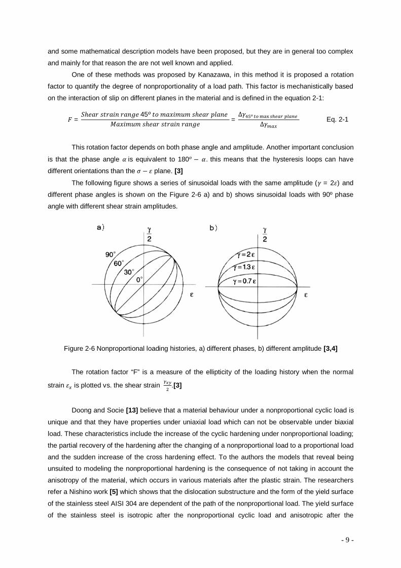
One of these methods was proposed by Kanazawa, in this method it is proposed a rotation
factor to quantify the degree of nonproportionality of a load path. This factor is mechanistically based
on the interaction of slip on different planes in the material and is defined in the equation 2-1:
This rotation factor depends on both phase angle and amplitude. Another important conclusion
is that the phase angle 훼 is equivalent to 180 − 훼. this means that the hysteresis loops can have
different orientations than the 휎 − 휀 plane. [3]
The following figure shows a series of sinusoidal loads with the same amplitude (훾 = 2휀) and
different phase angles is shown on the Figure 2-6 a) and b) shows sinusoidal loads with 90º phase
angle with different shear strain amplitudes.
Figure 2-6 Nonproportional loading histories, a) different phases, b) different amplitude [3,4]
The rotation factor “F” is a measure of the ellipticity of the loading history when the normal
strain 휀 is plotted vs. the shear strain .[3]
Doong and Socie [13] believe that a material behaviour under a nonproportional cyclic load is
unique and that they have properties under uniaxial load which can not be observable under biaxial
load. These characteristics include the increase of the cyclic hardening under nonproportional loading;
the partial recovery of the hardening after the changing of a nonproportional load to a proportional load
and the sudden increase of the cross hardening effect. To the authors the models that reveal being
unsuited to modeling the nonproportional hardening is the consequence of not taking in account the
anisotropy of the material, which occurs in various materials after the plastic strain. The researchers
refer a Nishino work [5] which shows that the dislocation substructure and the form of the yield surface
of the stainless steel AISI 304 are dependent of the path of the nonproportional load. The yield surface
of the stainless steel is isotropic after the nonproportional cyclic load and anisotropic after the
퐹 =푆ℎ푒푎푟 푠푡푟푎푖푛 푟푎푛푔푒 45º 푡표 푚푎푥푖푚푢푚 푠ℎ푒푎푟 푝푙푎푛푒
푀푎푥푖푚푢푚 푠ℎ푒푎푟 푠푡푟푎푖푛 푟푎푛푔푒 =∆훾 º
∆훾 Eq. 2-1

- 10 -
proportional load. In a previous work by Doong and Socie [13], it was proved that the partial
nonproportional hardening recovery and the material of the cross-hardening stainless steel is directly
related to the anisotropy of the material. In this work a cyclic plasticity model to metals under
nonproportional stress-torsion is presented and use a nonproportionality parameter based on the
strain path to give a close approach of the cyclic hardening level under a complex nonproportional
load. [3]
The nonproportional parameter 휙 proposed is defined by the equations 2-2 and 2-3
Where
Where 휀 – Plastic strain tensor
휈 – Constant to control the alteration ratio of the nonproportionality parameter
F – Weight function to reduce the contribution of the plastic work increment in the
integration calculus of the 휙 when the |휀 | is low
푑푤 – The cyclic nonproportionality stabilized parameter, obtained by integration
under a cycle. Its value can change in the next cycles but current cycle remains constant
Both relations which condition 푑휙 let the nonproportional parameter 휙 change with a cycle
load. The value 휙 increase from zero toward 휙 with a decreasing velocity. From the obtained results
the authors conclude that the hardening cyclic level foreseen by the nonproportionality parameter
agrees with the most of the experimental results, to a certain variety of load paths.[3]
Itoh [9] developed a wide research about the influence of the proportional and nonproportional
loadings on the materials hardening. The tests were made under strain controlled with a low number of
cycles, stainless steel type 304 specimens were tested at room temperature. From the different
variables in study it was observed: the rotation of the principal strains direction is the main factor in the
damage effect. With the fatigue life reduction reaching a factor of ten; if the number of steps in the load
path is low we have a larger influence in the hardening of the material, if the number of steps in the
path is high it can be approximated to a proportional load. The authors proposed an equivalent
nonproportional strain parameter, defined by:
푑휙 = 0 if 휙 ≤ 휙 Eq. 2-2
푑휙 = (휙 −휙) if 휙 > 휙 Eq. 2-3
휙 =∫ 퐹(|휀 |) 1− 휀
|휀 | : 푑휀|푑휀 | 푑푤
∫ 퐹(|휀 |) 1− 휀|휀 | : 푑휀|푑휀 | 푑푤
Eq. 2-4
Δ휀 = (1 + 훼푓 )Δ휀 Eq. 2-5
- 11 -
훼 is a material constant based on experimental results, related to the additional hardening under a
nonproportional loading delayed 90 degree and the 푓 is the nonproportional factor, obtain directly
from the strain path.[3]
Where:
휀 (푡) – Principal strain absolute value varies with time t
휀 – Maximum value of 휀 (푡)
휉(푡) – Angle between 휀 (푡) and 휀
T – Time per cycle
According to the authors the 푓 ratio can be calculated in the integral form based on the
experimental results, since under nonproportional low cycle fatigue the material is mainly influenced by
the change of the main strain direction angle of the principal strain and of the dimension of the strain
path after a change of direction in a representation √
휀. In a proportional load 푓 is zero. [3]
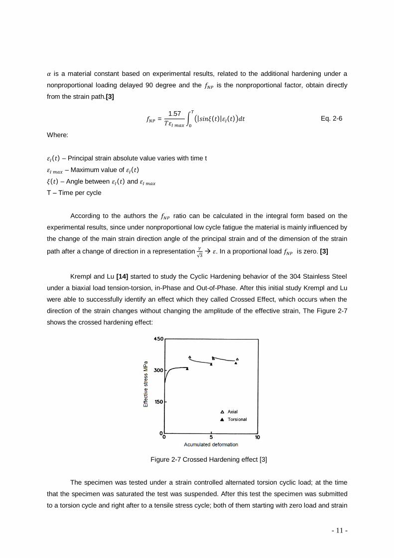
Krempl and Lu [14] started to study the Cyclic Hardening behavior of the 304 Stainless Steel
under a biaxial load tension-torsion, in-Phase and Out-of-Phase. After this initial study Krempl and Lu
were able to successfully identify an effect which they called Crossed Effect, which occurs when the
direction of the strain changes without changing the amplitude of the effective strain, The Figure 2-7
shows the crossed hardening effect:
Figure 2-7 Crossed Hardening effect [3]
The specimen was tested under a strain controlled alternated torsion cyclic load; at the time
that the specimen was saturated the test was suspended. After this test the specimen was submitted
to a torsion cycle and right after to a tensile stress cycle; both of them starting with zero load and strain
푓 =1.57푇휀
|푠푖푛휉(푡)|휀 (푡) 푑푡 Eq. 2-6
- 12 -
until an equivalent value to the effective strain is reached. With a cycle under axial load it was
achieved a reasonable increase to the stress amplitude. In the figure 2-7 after the axial load cycle the
effective stress amplitude starts to decrease, starting at the axial cycle stress amplitude, despite the
strain direction change, now we have torsion load cycle, an additional crossed effect is no longer
observed. The authors also said that this effect tend to diminish with the accumulated inelastic strain
and disappear after an Out-of-Phase cycle. This effect is caused by the process of anisotropy caused
by cyclic hardening and latent hardening.
Research for nonproportionality factors have been taken presented to account this effect. This
factor 퐹 , counts the effect of the nonproportionality, using the ratio between the semiminor axis and
the semimajor axis of the ellipse that surround the entire load. This factor is similar to the one
introduced differing only in the way of calculation. [3]
2.1.2. Additional Hardening
A lot of researchers observed that the amount of cyclic hardening substantially increases to
certain materials like copper and stainless steel due to nonproportional cyclic load. In addition to the
change of the stress state the nonproportinal loading creates additional cyclic hardening which is not
present in uniaxial tests. As a result the curve stress-strain for these materials in Out-of-Phase
loadings is superior to the In-Phase loads. In other way materials like the 6061-T6 shows the same
amount of hardening under a proportional or nonproportional cyclic load. And for that the increase of
the cyclic hardening due to nonproportional load depends on the material behavior, although this
material dependence can’t be explained only by the increase of the interaction of the dislocations due
to the rotation of the planes of maximum shear along with the nonproportional cycles. The difference
of the material behavior due to the cyclic hardening can be explained by the alterations that happen at
the level of the dislocations substructure, i.e. the increase of the cyclic stress to the nonproportional
cyclic behavior results of the alteration of the dislocations on the substructure of structures like single-
slip to multi-slip structures. Although the dislocation slip mechanism have a important part in the cyclic
hardening of the metals, it was considered necessary to research the effect of other strain
mechanisms, such as phase transformation induced by the stress. [3]
Additional hardening can happen due to the cyclic dislocations movement and the intersection
with active slip planes, which have origin on complex movements and dislocations of a large amount
of mechanisms of grain slip systems. It was also observed the influence of the materials internal
structure, this means that in the case of having a face centered cubic or a body centered cubic, it was
proved that the slip systems are easily activated in a b.c.c.. In the case of a hexagonal compact the
slip systems are lesser. [3]
The effect of changes on the strain direction can affect the cyclic strains at the micro and
macroscope level. To prove this statement a stainless steel 304 was tested, which shows a
dependence on the plastic strain amplitude starting on the metastable austenite (or gamma phase iron
(f.c.c.) to martensite alpha (b.c.c.) through the cycles. This material has a small value for stacking fault

- 13 -
energy (≅ 23 mJ/m ), promoting the formation of wide stacking fault and planar slip at room
temperature. The material shows a accentuate response to the cyclic hardening that depends on the
strain amplitude and on the strain nonproportionality in the plastic region. In this research the load
path (hardening material memory) and the additional cyclic strain hardening reveals to be more
dependent in nonproportional strain than plastic strain amplitude.
From the metallurgy viewpoint the observed additional hardening level is on a 90º out-of-
phase dependent on how easy the multiple slip systems evolves in a certain material. In materials with
low stacking fault energy and with widespread dislocations, only planar slips systems evolve under a
proportional load. However during a nonproportional load the maximum stress planes rotate causing a
plastic strain through the different slip mechanisms. The cross-slip activation, due to plastic strain can
result in a significant increase of the hardening when compared with a uniaxial load or proportional
cyclic. [3]
Materials with high stacking fault energy and with dislocations next to each others, the slip is
easy and occurs in both proportional and nonproportional loads. The additional hardening is not visible
in these materials during the nonproportional strain because a significant slip occurs also in a
proportional load. As an example we have the Aluminum which has stacking fault energy of 250 푚퐽/
푚 , and so this material virtually shows the same stress-strain curve independent of the proportionality
of the load path. A significant slip occurs in the Aluminum independently of the aspect and path of
strain.
2.2. Low Cycle Fatigue Behaviour
This phenomenon is related to the rupture which can occur in a component or structure in a
number of cycles usually below 10 − 10 . In this situation the material is under levels of stress/strain
above the elastic limit.
2.2.1. Uniaxial and Biaxial
When an elasto-plastic material is submitted to a cyclic load, the load path (stress and strain)
has a transition state which tends toward a steady state cycle. In the steady state cycle the material
behavior can be characterized by four different modes which depend on the load path influence:
1. Elastic: the stress maintains elastic linear along all the cycle and doesn’t occur in plastic
strains.
2. Elastic shakedown: appears some plastic strains during the initial load phase followed by a
purely elastic response.
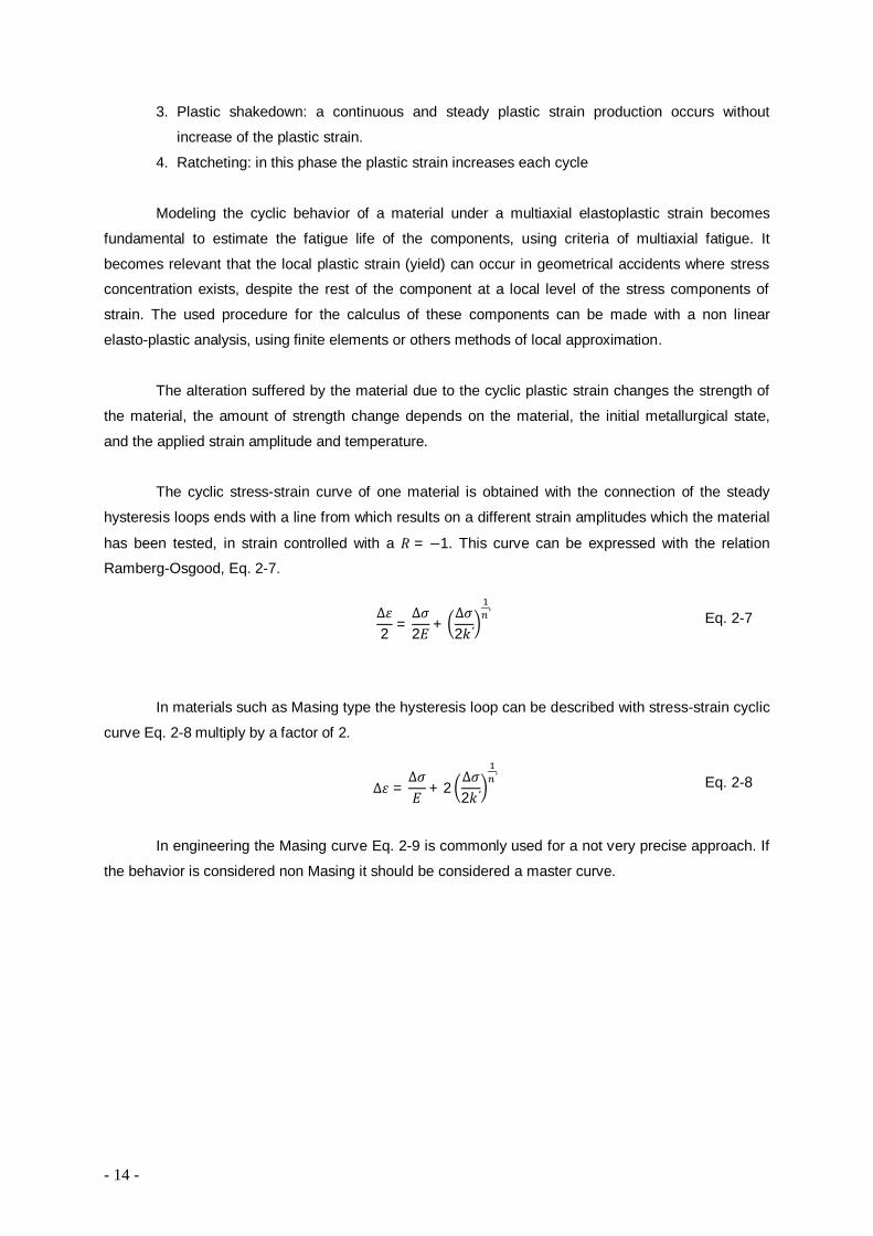
- 14 -
3. Plastic shakedown: a continuous and steady plastic strain production occurs without
increase of the plastic strain.
4. Ratcheting: in this phase the plastic strain increases each cycle
Modeling the cyclic behavior of a material under a multiaxial elastoplastic strain becomes
fundamental to estimate the fatigue life of the components, using criteria of multiaxial fatigue. It
becomes relevant that the local plastic strain (yield) can occur in geometrical accidents where stress
concentration exists, despite the rest of the component at a local level of the stress components of
strain. The used procedure for the calculus of these components can be made with a non linear
elasto-plastic analysis, using finite elements or others methods of local approximation.
The alteration suffered by the material due to the cyclic plastic strain changes the strength of
the material, the amount of strength change depends on the material, the initial metallurgical state,
and the applied strain amplitude and temperature.
The cyclic stress-strain curve of one material is obtained with the connection of the steady
hysteresis loops ends with a line from which results on a different strain amplitudes which the material
has been tested, in strain controlled with a 푅 = −1. This curve can be expressed with the relation
Ramberg-Osgood, Eq. 2-7.
In materials such as Masing type the hysteresis loop can be described with stress-strain cyclic
curve Eq. 2-8 multiply by a factor of 2.
In engineering the Masing curve Eq. 2-9 is commonly used for a not very precise approach. If
the behavior is considered non Masing it should be considered a master curve.
∆휀2 =
∆휎2퐸 +
∆휎2푘 ′
′ Eq. 2-7
∆휀 =∆휎퐸 + 2
∆휎2푘 ′
′ Eq. 2-8

- 15 -
Figure 2-8 Possible material behavior to monotonic curves and steady cycles [3]
The strain-life curves, Coffin and Manson relates the strain amplitude of the plastic component
and the number of the cycles until the rupture, and Basquin proposed an expression which relates the
strain elastic component and the number of cycles 2푁 . Later, Morrow shows that the metals strength
to fatigue under a certain total strain amplitude can be expressed by the elastic and plastic strain
component. The equation proposed relates the life fatigue in a LCF or a HCF: [3, 4]
The study of the low cycle fatigue behavior and materials under multiaxial fatigue loading,
more particularly cyclic cases of stress/compression with cyclic torsion, have been lately studied by
various researchers. [3]
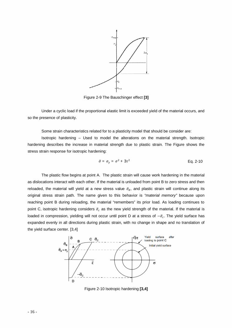
2.2.2. Isotropic and Kinematic Hardening
Under monotonic or proportional stress loads the plastic hardening models, isotropic and
kinematic, present similar results, when a reversible load is present the same is not true because the
results differ substantially. Since the research by the pioneer Bauschinger is known that the reverse
plastic strain is associated to the fatigue damage.
∆휀2 =
휎 ′ − 휎퐸 + 휀 ′ 2푁 Eq. 2-9
- 16 -
Figure 2-9 The Bauschinger effect [3]
Under a cyclic load if the proportional elastic limit is exceeded yield of the material occurs, and
so the presence of plasticity.
Some strain characteristics related for to a plasticity model that should be consider are:
Isotropic hardening – Used to model the alterations on the material strength. Isotropic
hardening describes the increase in material strength due to plastic strain. The Figure shows the
stress strain response for isotropic hardening:
The plastic flow begins at point A. The plastic strain will cause work hardening in the material
as dislocations interact with each other. If the material is unloaded from point B to zero stress and then
reloaded, the material will yield at a new stress value 휎 , and plastic strain will continue along its
original stress strain path. The name given to this behavior is “material memory” because upon
reaching point B during reloading, the material “remembers” its prior load. As loading continues to
point C, isotropic hardening considers 휎 as the new yield strength of the material. If the material is
loaded in compression, yielding will not occur until point D at a stress of −휎 . The yield surface has
expanded evenly in all directions during plastic strain, with no change in shape and no translation of
the yield surface center. [3,4]
Figure 2-10 Isotropic hardening [3,4]
휎 = 휎 = 휎 + 3휏 Eq. 2-10
- 17 -
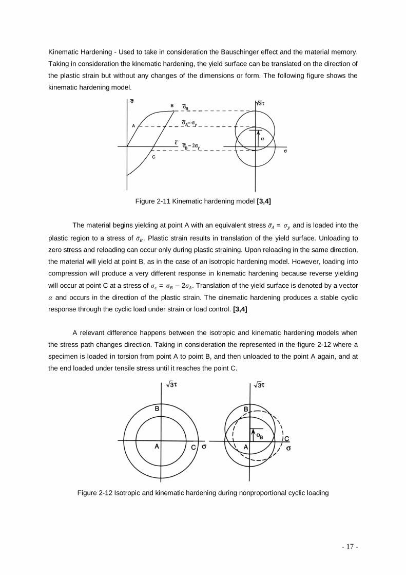
Kinematic Hardening - Used to take in consideration the Bauschinger effect and the material memory.
Taking in consideration the kinematic hardening, the yield surface can be translated on the direction of
the plastic strain but without any changes of the dimensions or form. The following figure shows the
kinematic hardening model.
Figure 2-11 Kinematic hardening model [3,4]
The material begins yielding at point A with an equivalent stress 휎 = 휎 and is loaded into the
plastic region to a stress of 휎 . Plastic strain results in translation of the yield surface. Unloading to
zero stress and reloading can occur only during plastic straining. Upon reloading in the same direction,
the material will yield at point B, as in the case of an isotropic hardening model. However, loading into
compression will produce a very different response in kinematic hardening because reverse yielding
will occur at point C at a stress of 휎 = 휎 − 2휎 . Translation of the yield surface is denoted by a vector
훼 and occurs in the direction of the plastic strain. The cinematic hardening produces a stable cyclic
response through the cyclic load under strain or load control. [3,4]
A relevant difference happens between the isotropic and kinematic hardening models when
the stress path changes direction. Taking in consideration the represented in the figure 2-12 where a
specimen is loaded in torsion from point A to point B, and then unloaded to the point A again, and at
the end loaded under tensile stress until it reaches the point C.
Figure 2-12 Isotropic and kinematic hardening during nonproportional cyclic loading
- 18 -
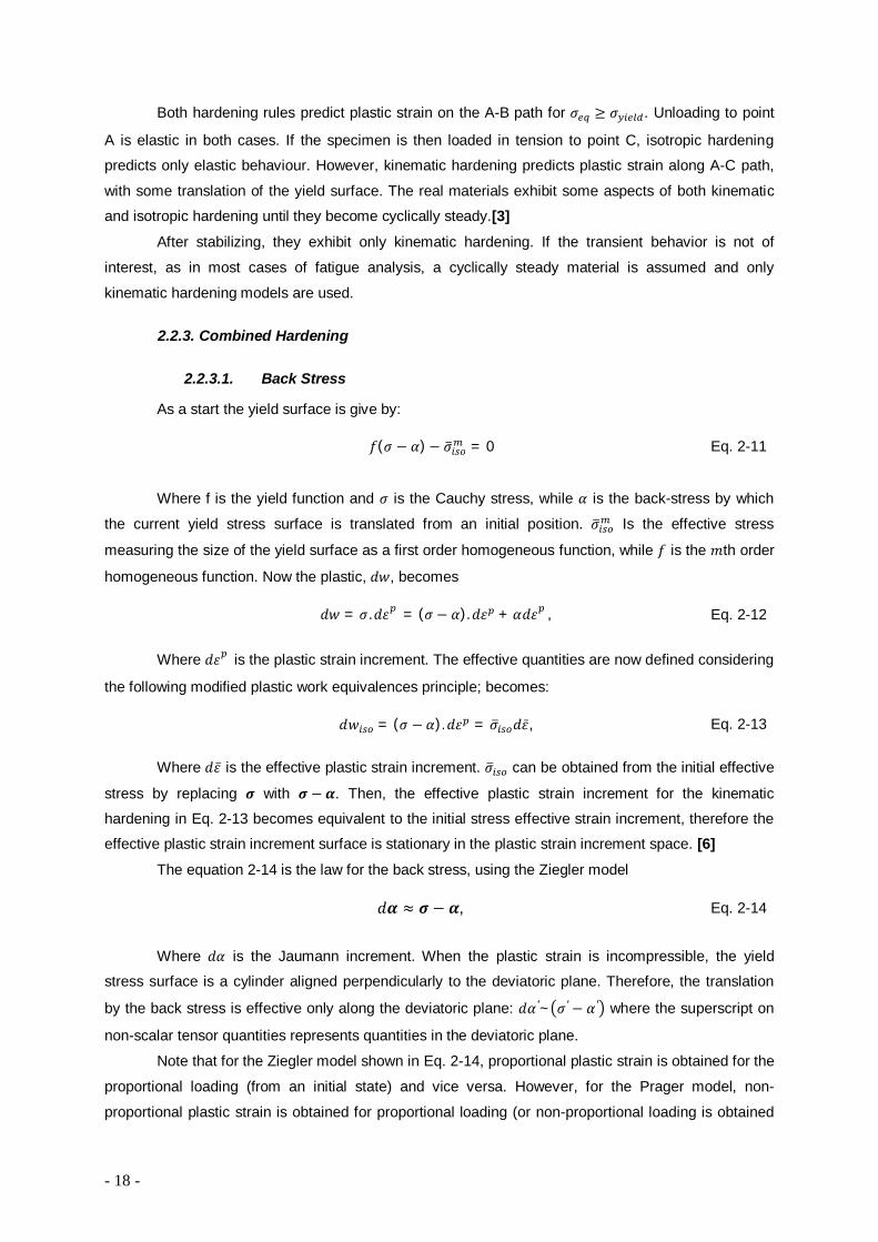
Both hardening rules predict plastic strain on the A-B path for 휎 ≥ 휎 . Unloading to point
A is elastic in both cases. If the specimen is then loaded in tension to point C, isotropic hardening
predicts only elastic behaviour. However, kinematic hardening predicts plastic strain along A-C path,
with some translation of the yield surface. The real materials exhibit some aspects of both kinematic
and isotropic hardening until they become cyclically steady.[3]
After stabilizing, they exhibit only kinematic hardening. If the transient behavior is not of
interest, as in most cases of fatigue analysis, a cyclically steady material is assumed and only
kinematic hardening models are used.
2.2.3. Combined Hardening
2.2.3.1. Back Stress
As a start the yield surface is give by:
Where f is the yield function and 휎 is the Cauchy stress, while 훼 is the back-stress by which
the current yield stress surface is translated from an initial position. 휎 Is the effective stress
measuring the size of the yield surface as a first order homogeneous function, while 푓 is the 푚th order
homogeneous function. Now the plastic, 푑푤, becomes
Where 푑휀 is the plastic strain increment. The effective quantities are now defined considering
the following modified plastic work equivalences principle; becomes:
Where 푑휀 is the effective plastic strain increment. 휎 can be obtained from the initial effective
stress by replacing 흈 with 흈 − 휶. Then, the effective plastic strain increment for the kinematic
hardening in Eq. 2-13 becomes equivalent to the initial stress effective strain increment, therefore the
effective plastic strain increment surface is stationary in the plastic strain increment space. [6]
The equation 2-14 is the law for the back stress, using the Ziegler model
Where 푑훼 is the Jaumann increment. When the plastic strain is incompressible, the yield
stress surface is a cylinder aligned perpendicularly to the deviatoric plane. Therefore, the translation
by the back stress is effective only along the deviatoric plane: 푑훼 ′~ 휎′ − 훼 ′ where the superscript on
non-scalar tensor quantities represents quantities in the deviatoric plane.
Note that for the Ziegler model shown in Eq. 2-14, proportional plastic strain is obtained for the
proportional loading (from an initial state) and vice versa. However, for the Prager model, non-
proportional plastic strain is obtained for proportional loading (or non-proportional loading is obtained
푓(휎 − 훼)− 휎 = 0 Eq. 2-11
푑푤 = 휎.푑휀 = (휎 − 훼). 푑휀 + 훼푑휀 , Eq. 2-12
푑푤 = (휎 − 훼).푑휀 = 휎 푑휀, Eq. 2-13
푑휶 ≈ 흈 − 휶, Eq. 2-14

- 19 -
for proportional plastic strain. An exceptional case is found for the Mises yield stress surface, in which
Eq.’s 2-14 and 2-15 are equivalent; i.e. 휎 ′ − 훼 ′ ~푑휀 . [6]
As for the effective back-stress increment, 푑훼, the value is obtained from the initial effective
stress by replacing 휎 with 푑훼. The definitions of the effective quantities for the stress, the conjugate
plastic strain increment, and the back-stress increment are for any anisotropic yield stress surfaces,
which are first-order homogeneous functions.
Usual assumptions:
Additive decoupling into elastic and incompressible plastic strain increments, 푑휀 = 푑휀 + 푑휀 ,
and associate flow rule based on the normality rule. For the plane stress strain of sheets with the
condition that 휎 = 휎 = 휎 = 0 and the 푑휀 = 푑휀 = 푑휀 = 푑휀 = 0, the constitutive law can be
effectively handled considering the 3D yield surface in the 휎 , 휎 , 휎 stress and the 푑휀 , 푑휀 , 푑휀
strain increment spaces, without considering deviatoric values: the plane stress field. Besides, the
increment condition provides 푑휀 = 푑휀 − 푑휀 for the plastic strain and 푑휀 = 푑휀 + 푑휀 for
the isotropic elastic strain with the Poisson’s ration,휈. [6] Note that when the formulation is expressed in the plane stress field, the back stress evolution
for the Prager model shown in Eq. 2-15 becomes:
This represents the translation on the plane stress field. For the simple tension of the Mises material,
푑휀 :푑휀 :푑휀 = 1: 0: 0 in the plane stress field, while 푑휀 :푑휀 :푑휀 = 2:−1:−1 in the deviatoric
plane, which complies with the fact the Prager and Ziegler models are identical. [6]
2.2.3.2. Flow formulation of Chaboche model
Chaboche model is an intrinsic formulation on the ABAQUS. A short summary of this method
is given:
The yield surface is described by Eq. 2-16 where 휎 is the value measuring the size of the
yield surface as a function of the effective strain, 휀(∫푑휀). Therefore, Eq. 2-16 leads to
푑훼 =푑훼푑훼푑훼
~푑휀 =푑휀 − 푑휀푑휀 − 푑휀
푑휀=
2푑휀 + 푑휀푑휀 + 푑휀
푑휀 Eq. 2-15
휕푓
휕(휎 − 훼)푑휎 −휕푓
휕(휎 − 훼)푑훼 −푚휎휕휎휕휀
(휎 − 훼).푑휀 = 0 Eq. 2-16
- 20 -
In the Chaboche model, the back-stress increment is composed of two terms, 푑훼 = 푑훼 − 푑훼
to differentiate the transient hardening behavior during loading and unloading (or reverse loading).
Therefore,
Where
The magnitude of the back stress increments in Eq. 2-18 is obtained by substituting the back
stress into the yield function 푓. Then the equation takes the form of the Eq. 2-19
rearranging 푑훼 = 푓(푑휶 ) and therefore:
And for 푑휶 :
푑훼 and 푑휶 can be generalized to tensor quantities to account for the directional difference off the
back stress for highly anisotropic materials.
The plastic strain increment can be consider as:
Linear isotropic elastic constitutive law is based on Eq.2-11 and is given by:
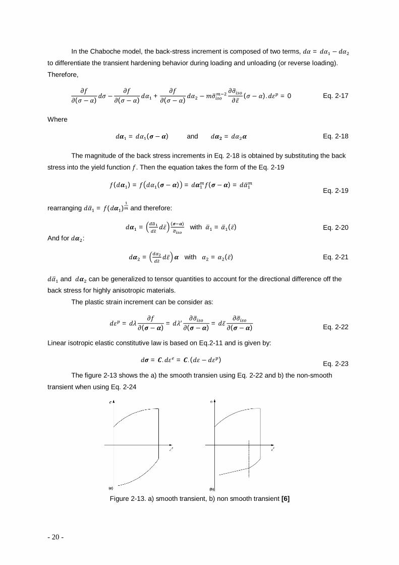
The figure 2-13 shows the a) the smooth transien using Eq. 2-22 and b) the non-smooth
transient when using Eq. 2-24
Figure 2-13. a) smooth transient, b) non smooth transient [6]
휕푓휕(휎 − 훼) 푑휎 −
휕푓휕(휎 − 훼)푑훼 +
휕푓휕(휎 − 훼)푑훼 − 푚휎
휕휎휕휀
(휎 − 훼). 푑휀 = 0 Eq. 2-17
푑휶 = 푑훼 (흈− 휶) and 푑휶ퟐ = 푑훼 휶 Eq. 2-18
푓(푑휶 ) = 푓 푑훼 (흈− 휶) = 푑휶 푓(흈 − 휶) = 푑훼
Eq. 2-19
푑휶 = 푑휀 (흈 휶) with 훼 = 훼 (휀) Eq. 2-20
푑휶 = 푑휀 휶 with 훼 = 훼 (휀) Eq. 2-21
푑휀 = 푑휆휕푓
휕(흈− 휶) = 푑휆휕휎
휕(흈 − 휶) = 푑휀휕휎
휕(흈 − 휶)
Eq. 2-22
푑흈 = 푪. 푑휀 = 푪. (푑휀 − 푑휀 ) Eq. 2-23

- 21 -
Using the Eq’s 2-20, 2-23, 2-18 to 훼 comes in the form of Eq. 2-24:
Where ℎ = , is the slope of the 휎 (휀) curve. Using the Eq 2-24 becomes the Eq.2-25
And
For a strain increment, 푑휀, prescribed at every time increment, Eqs. 2-22 and 2-26 determine
the plastic strain increment and then the back-stress and Cauchy can be updated to the Jaumann
stress increments as shown in Eq’s 2-20, 2-23, 2-18, respectively. [6]
Cyclic creep or ratchetting - can be defined as the accumulation of plastic strain and is
observed in materials that are subjected to a mean stress. Consider a thin-walled tube under a cycle
of shear strain with a static axial stress. The magnitude of the cyclic shear strain is large enough to
produce plastic strain during each cycle. And during each cycle, the total axial strain continues to
increase as illustrated by the test results in Figure 2-14, which shows a plot of shear strain versus axial
strain.
Both axial and shear strain are increased to point A when the initial loads are applied. The
shear strain is cyclic, while the axial stress is held constant. The axial strain remains constant during
the elastic portion of loading to point B. After this, plastic strain occurs, and there is coupling between
the axial strain and shear loading. During a plastic loading, shear loads also produce axial strain. No
axial strain is produced in the elastic amplitude. In this example, the ratcheting rate decreases, and
strain eventually becomes stable. For large plastic strains the ratcheting rate increases with each
cycle. [3,4]
휕푓휕(휎 − 훼)푪 푑휀 −
휕푓휕(휎 − 훼)푪푑휀 +
휕푓휕(흈 − 휶)
푑훼휎
(훔 − 훂) +휕푓
휕(흈 − 휶)푑훼 휶
= 푚휎 ℎ (흈 − 휶)푑휀
Eq. 2-24
푑휆 =
휕푓휕(흈 − 휶) 푪푑휀 − 푑훼1(푚휎푖푠표푚−1) + 푑훼2
휕푓휕(흈 − 휶)휶
휕푓휕(흈 − 휶)푪
휕푓휕(흈 − 휶) + 푚2휎푖푠표2푚−2ℎ푖푠표
=
휕휎푖푠표휕(흈 − 휶) 푪푑휀 − 푑훼1 + 푑훼2
휕휎푖푠표휕(흈 − 휶)휶
휎푖푠표푚−1 휕휎푖푠표휕(흈 − 휶) 푪
휕휎푖푠표휕(흈 − 휶) + ℎ푖푠표
Eq. 2-25
푑휆 =
휕휎푖푠표휕(흈 − 휶) 푪푑휀 − 푑훼1 + 푑훼2
휕휎푖푠표휕(흈 − 휶)휶
휕휎푖푠표휕(흈 − 휶)푪
휕휎푖푠표휕(흈 − 휶) + ℎ푖푠표
Eq. 2-26
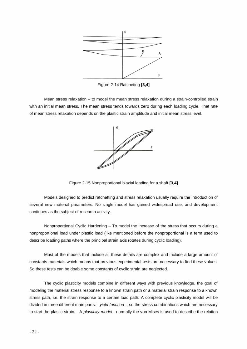
- 22 -
Figure 2-14 Ratcheting [3,4]
Mean stress relaxation – to model the mean stress relaxation during a strain-controlled strain
with an initial mean stress. The mean stress tends towards zero during each loading cycle. That rate
of mean stress relaxation depends on the plastic strain amplitude and initial mean stress level.
Figure 2-15 Nonproportional biaxial loading for a shaft [3,4]
Models designed to predict ratchetting and stress relaxation usually require the introduction of
several new material parameters. No single model has gained widespread use, and development
continues as the subject of research activity.
Nonproportional Cyclic Hardening – To model the increase of the stress that occurs during a
nonproportional load under plastic load (like mentioned before the nonproportional is a term used to
describe loading paths where the principal strain axis rotates during cyclic loading).
Most of the models that include all these details are complex and include a large amount of
constants materials which means that previous experimental tests are necessary to find these values.
So these tests can be doable some constants of cyclic strain are neglected.
The cyclic plasticity models combine in different ways with previous knowledge, the goal of
modeling the material stress response to a known strain path or a material strain response to a known
stress path, i.e. the strain response to a certain load path. A complete cyclic plasticity model will be
divided in three different main parts: - yield function -, so the stress combinations which are necessary
to start the plastic strain. - A plasticity model - normally the von Mises is used to describe the relation

- 23 -
between the stress and the plastic strain, it’s also a constitutive equation used to describe the relation
between stress and the plastic strain increments, and at last a - hardening model -, used to describe
how the yield criterion (yield surfaces) varies with the plastic strain. [3]
2.3. Biaxial Fatigue Life Prediction Theories
The critical plane models have been developed through the last years, and they are used to
predict life of the nucleation and the beginning of the crack growth to apply in multiaxial fatigue
problems. All the theories include a maximum plane of the material where should occur the maximum
critical damage due to Axial and shear stresses, the so called Critical Plane.
The procedure includes two phases, in the first one the critical plane is calculated considering
the values of the axial and shear stress in each plane of the material, in a second phase it will be
verified if the criterion is satisfied or not. If the criterion is satisfied this will be the potential plane where
a fatigue crack should start. Therefore the initial orientation coincides with the orientation of the critical
plane.
Depending on the material the stress state, the environment and of the strain amplitude, the
fatigue life will be dominated by the crack growth, through the shear planes or through the tensile
stress planes. A critical plane mode includes the parameters which define the type of the crack growth.
This type of model to be well succeeded must be ready to estimate reasonably the fatigue life and the
crack plane dominant. Due to the different possibilities of crack modes, where shear stress or tensile
stress can be dominant, it can’t be predicted if a simple model can correlate the results to all materials
in all fatigue life regimes. [3]
2.3.1. Findley model
Based on physical observation of the initial orientation of the fatigue cracks on steel, and
Aluminum, they discuss the influence of the normal stress on the plane where the shear stress
maximum. According to the Findley model the normal stress, acting on a plane can change linearly the
alternated shear stress available on that plane. The failure will not occur if:
From here the resulting proposal of the critical plane model which predicts the plane where the
crack initiates is the plane with a certain orientation 휃 that originates the maximum damage parameter:
Where 휏 is the shear stress amplitude on a plane 휃, mean maximum stress on the 휃 plane and
k is a constant of the material. The k constant can be determined experimentally with fatigue tests
which involve two or more stress states, for e.g. pure torsion and pure flexion, where it will be
obtained:
∆휏2 + 푘휎 ≤ 푓 Eq. 2-27
max 휏 + 푘휎 , Eq. 2-28
- 24 -
That means:
Findley identifies a critical plane to the crack begin and growth which depends of both
stresses, i.e. alternate shear stress and maximum normal stress. The combination of these two
stresses is responsible of the fatigue damage and the maximum value between brackets is used
instead of the maximum shear stress. The mean stress effects are taken in account on the normal
stress plane 휃.
A criterion based on the stress is adequate to predict long life fatigue project, therefore is also
used in the case of shorter life, in this case the relation to consider will be:
Where 휏∗ is calculated using the resistance coefficient to the torsion fatigue [3,4]
2.3.2. Brown Miller Model
This model is based on several multiaxial low cycle fatigue studies available and particularly
emphasis on the formation and initial crack growth. Octahedral shear stress in some cases proved to
be effective to correlate the crack under high cycle fatigue, the octahedral shear strain and the
maximum shear strain prove to be not effective related to the low cycle fatigue. The research included
combined torsion tension with a constant distortion, ∆훾 = constant. After reviewing the results it was
concluded that were needed two strain parameters to describe the fatigue process.
Analogous to the Findley shear and normal stress under high cycle fatigue, Brown and Miller
proposed that should be considered both shear and normal cyclic strain, on the plane where the
maximum shear strain occurs. The cyclic shear strain promotes the crack nucleation and the normal
strain influence its growth. Two types of cracks came up:
√1 + 푘 ∆ = 푓 and:
Eq. 2-29
휎 + 푘 휎 + 푘휎 = 2푓 Eq. 2-30
휎 ,
휏 ,=
2
1 + 푘√1 + 푘
Eq. 2-31
∆휏2 + 푘휎 = 휏∗ 푁 Eq. 2-32
휏∗ = 1 + 푘 휏 Eq. 2-33

- 25 -
Figure 2-16 Crack type A and B [3]
Crack type A: where 휆 = < 0 the shear stress occurs on the free surface, in a parallel
direction to the crack length. As a result of this crack types it tends to maintain and growing through
the surface (not deep cracks) and having small dimensions. In the case of cracks type B, where
휆 = > 0 under biaxial stress, the shear stress acts in a way to increase the crack.
This crack type most of the times intercepts the surface through a 45º angle. The type B is
more severe than type A. A material under combined stress torsion usually creates cracks type A, and
a biaxial load under axial stress will create cracks of the type B.
Different models were developed by Brown Miller [15] for each cracking type:
The values g and h are constants to determine. The value j varies from 1 (brittle materials) to 2
(ductile materials). Later this model would develop with some proposals made by Kandil, Wang and
Brown, to simplify the formulation of the type A cracks and to take in consideration the effects of the
mean stress.
The S parameter depends on the material and represents the influence of the normal strain on
the crack growth, and is determined with the correlation of the experimental results under tension and
torsion. Near the fatigue life limit, S will be approximately 0.3 to ductile materials. Note: the mean
stress is included is on the right part of the Eq. 2-36.
Type A cracks ∆ + = 1 Eq. 2-34
Type B cracks ∆ = 푐표푛푠푡 Eq. 2-35
∆훾2 + 푆∆휀 = (1.3 + 0.7푆)
휎 ′ − 2휎 ,
퐸 2푁 + (1.5 + 0.5푆)휀 ′ 2푁 Eq. 2-36
surface
A
B
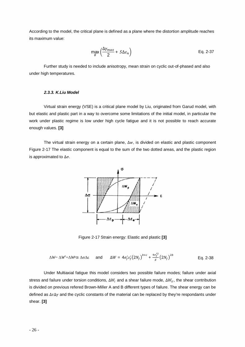
- 26 -
According to the model, the critical plane is defined as a plane where the distortion amplitude reaches
its maximum value:
Further study is needed to include anisotropy, mean strain on cyclic out-of-phased and also
under high temperatures.
2.3.3. K.Liu Model
Virtual strain energy (VSE) is a critical plane model by Liu, originated from Garud model, with
but elastic and plastic part in a way to overcome some limitations of the initial model, in particular the
work under plastic regime is low under high cycle fatigue and it is not possible to reach accurate
enough values. [3]
The virtual strain energy on a certain plane, ∆푤, is divided on elastic and plastic component
Figure 2-17 The elastic component is equal to the sum of the two dotted areas, and the plastic region
is approximated to ∆휎.
Figure 2-17 Strain energy: Elastic and plastic [3]
Under Multiaxial fatigue this model considers two possible failure modes; failure under axial
stress and failure under torsion conditions, ∆푊 and a shear failure mode, ∆푊 , the shear contribution
is divided on previous refered Brown-Miller A and B different types of failure. The shear energy can be
defined as ∆휏∆훾 and the cyclic constants of the material can be replaced by they’re respondants under
shear. [3]
max∆훾
2+ 푆∆휀 Eq. 2-37
ΔW= ΔWe+ΔWp≅ ΔσΔε and ∆푊 = 4휎 휀 2푁 + 2푁 Eq. 2-38
- 27 -
The failure should occur on a plane 휃 where the VSE is maximum. To determine the failure
mode under tensile stress ∆푊 is calculated and that way 휃 can be identified, where the axial energy is
maximized and summed to the respective shear stress on that plane. The description is translated on
the following equation:
To predict fatigue life it comes in the form of:
Similarly, ∆푊 is determined after identifying the plane 휃 where the shear energy is
maximized, adding the axial energy on the same plane, we obtain the equation:
To predict fatigue life it comes in the form of:
Where Δσn is the axial stress amplitude and Δεn is the normal strain amplitude, ∆휏 is the shear
stress amplitude ∆훾 is the distortion, G is the modulus of transversal elasticity, 휏 ′ the fatigue shear
strength coefficient, 훾 ′ the fatigue ductility coefficient, 푏 is the fatigue strength exponent and 푐 the
fatigue ductility exponent. Subscript max means that the value between brackets is the maximum
value of all 휃 planes.
The model parameters under mode II for both crack types A is designated as ∆푊 , and B is
∆푊 , . Under mode I there is only one critical plane, under the mode II there are two different critical
90º out-of-phase planes. Under uniaxial loads are designated as ∆푊 , = ∆푊 , . Under torsion or
Tension-Torsion ∆푊 , > ∆푊 , . The VSE are essentially critical plane models with energy basis, and
they are physically associated to two different fatigue failures. Depending on the material, the
temperature, the load and one of these three VSE parameters: ∆푊, ∆푊 , and ∆푊 , . Both
parameters ∆푊 and ∆푊 are virtual quantities and altough they can be identified they are not the
same as the elastic and plastic strain energy. [3,4]
2.3.4. Smith, Watson and Topper (S-W-T) Model
For materials where the failure is predominantly due to maximum tensile strain or stress crack
growth, S-W-T is a more suitable critical plane method; this model was originally developed as a
∆푊 = (∆휎 ∆휀 ) max +(∆휏∆훾) Eq. 2-39
∆푊 = 4휎 ′ 휀 ′ 2푁 +4휎 ′
퐸 2푁 Eq. 2-40
∆푊 = (∆휎 ∆휀 ) +(∆휏∆훾)max Eq. 2-41
∆푊 = 4휏 ′ 훾 ′ 2푁 +4휏 ′
퐺 2푁 Eq. 2-42
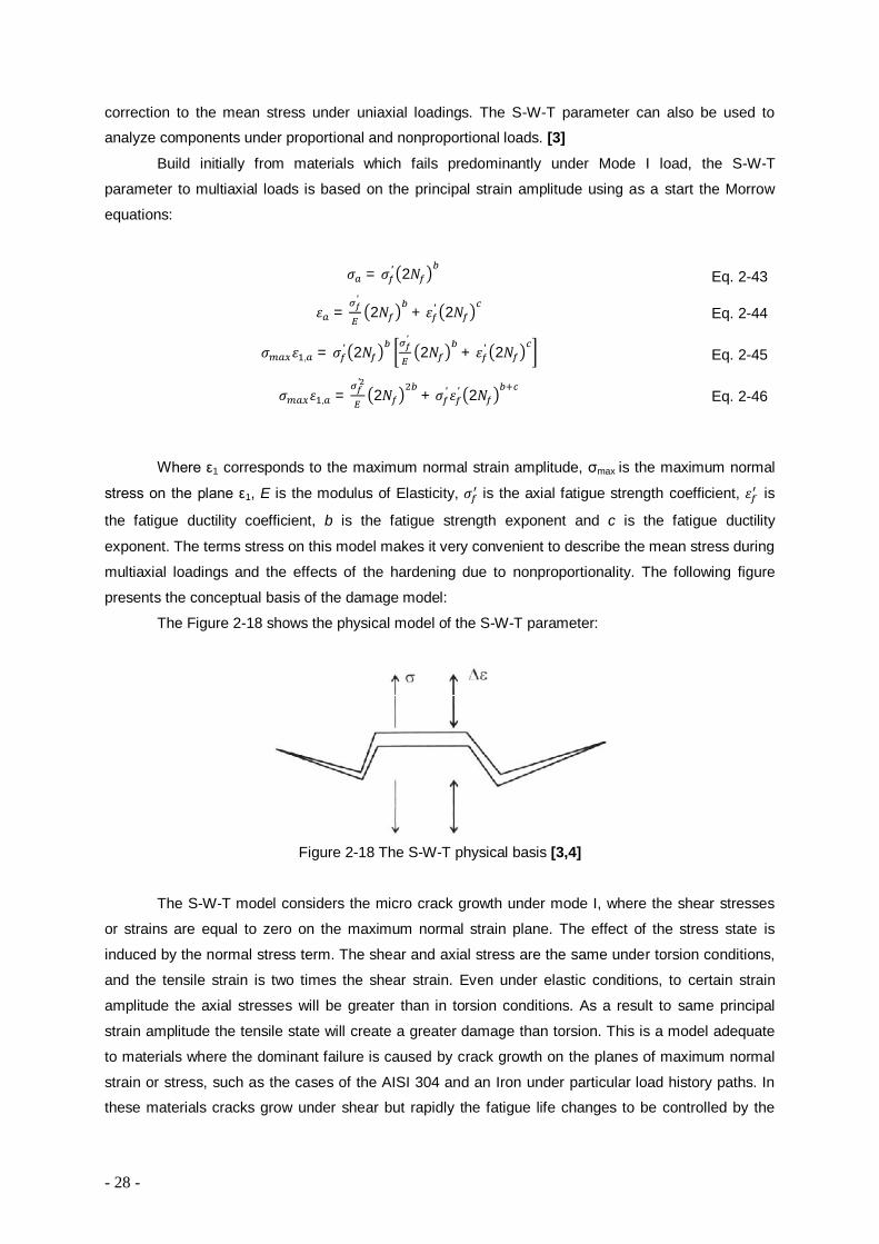
- 28 -
correction to the mean stress under uniaxial loadings. The S-W-T parameter can also be used to
analyze components under proportional and nonproportional loads. [3]
Build initially from materials which fails predominantly under Mode I load, the S-W-T
parameter to multiaxial loads is based on the principal strain amplitude using as a start the Morrow
equations:
Where ε1 corresponds to the maximum normal strain amplitude, σmax is the maximum normal
stress on the plane ε1, E is the modulus of Elasticity, 휎 is the axial fatigue strength coefficient, 휀 is
the fatigue ductility coefficient, b is the fatigue strength exponent and c is the fatigue ductility
exponent. The terms stress on this model makes it very convenient to describe the mean stress during
multiaxial loadings and the effects of the hardening due to nonproportionality. The following figure
presents the conceptual basis of the damage model:
The Figure 2-18 shows the physical model of the S-W-T parameter:
Figure 2-18 The S-W-T physical basis [3,4]
The S-W-T model considers the micro crack growth under mode I, where the shear stresses
or strains are equal to zero on the maximum normal strain plane. The effect of the stress state is
induced by the normal stress term. The shear and axial stress are the same under torsion conditions,
and the tensile strain is two times the shear strain. Even under elastic conditions, to certain strain
amplitude the axial stresses will be greater than in torsion conditions. As a result to same principal
strain amplitude the tensile state will create a greater damage than torsion. This is a model adequate
to materials where the dominant failure is caused by crack growth on the planes of maximum normal
strain or stress, such as the cases of the AISI 304 and an Iron under particular load history paths. In
these materials cracks grow under shear but rapidly the fatigue life changes to be controlled by the
휎 = 휎 ′ 2푁 Eq. 2-43
휀 =′
2푁 + 휀 ′ 2푁 Eq. 2-44
휎 휀 , = 휎 ′ 2푁′
2푁 + 휀 ′ 2푁 Eq. 2-45
휎 휀 , =′
2푁 + 휎 ′ 휀 ′ 2푁 Eq. 2-46
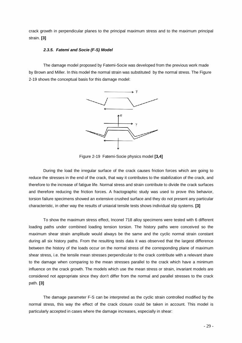
- 29 -
crack growth in perpendicular planes to the principal maximum stress and to the maximum principal
strain. [3]
2.3.5. Fatemi and Socie (F-S) Model
The damage model proposed by Fatemi-Socie was developed from the previous work made
by Brown and Miller. In this model the normal strain was substituted by the normal stress. The Figure
2-19 shows the conceptual basis for this damage model:
Figure 2-19 Fatemi-Socie physics model [3,4]
During the load the irregular surface of the crack causes friction forces which are going to
reduce the stresses in the end of the crack, that way it contributes to the stabilization of the crack, and
therefore to the increase of fatigue life. Normal stress and strain contribute to divide the crack surfaces
and therefore reducing the friction forces. A fractographic study was used to prove this behavior,
torsion failure specimens showed an extensive crushed surface and they do not present any particular
characteristic, in other way the results of uniaxial tensile tests shows individual slip systems. [3]
To show the maximum stress effect, Inconel 718 alloy specimens were tested with 6 different
loading paths under combined loading tension torsion. The history paths were conceived so the
maximum shear strain amplitude would always be the same and the cyclic normal strain constant
during all six history paths. From the resulting tests data it was observed that the largest difference
between the history of the loads occur on the normal stress of the corresponding plane of maximum
shear stress, i.e. the tensile mean stresses perpendicular to the crack contribute with a relevant share
to the damage when comparing to the mean stresses parallel to the crack which have a minimum
influence on the crack growth. The models which use the mean stress or strain, invariant models are
considered not appropriate since they don’t differ from the normal and parallel stresses to the crack
path. [3]
The damage parameter F-S can be interpreted as the cyclic strain controlled modified by the
normal stress, this way the effect of the crack closure could be taken in account. This model is
particularly accepted in cases where the damage increases, especially in shear:
- 30 -
Where ∆ is the maximum shear strain amplitude and 휎 , is normal stress corresponding
to the maximum shear strain amplitude, 휎 is the yield stress of the monotonic curve, k is a constant of
the material, which can be determined with the correlation of the experimental results under uniaxial
fatigue tension/compression and under torsion, 훾 the shear fatigue ductility coefficient, 푏 the shear
fatigue strength exponent and 푐 is the shear fatigue ductility exponent. Properties can be calculated
from torsion fatigue tests, or can be estimated by the following equations using the axial properties:
This model tries to explain the difference between a tension and a torsion load case, besides
it’s possible to consider the effects of the mean normal stress and the additional hardening caused by
the nonproportionality using the normal stress term. The critical plane model which includes only the
strain components cannot reflect the effects of the mean stress or the strain paths influence on the
hardening. The F-S model is indicated to materials where the loading conditions result in failure due to
shear stresses. To nonproportional multiaxial loads where the principal directions rotate a new critical
plane, is given by the plane where the greater damage parameter occurs:
Instead of the previous one where it was considered the damage on the plane of the maximum shear
strain amplitude. [3]
2.4. Additional research
In 2000 a simple approach to the description of multiaxial cyclic stress-strain relationship,
using the critical plane and the research results of multiaxial critical plane principle, it was propose that
the normal strain excursion 휀∗ between adjacent turning points of the maximum strain and the
maximum shear strain amplitude 훾 on the critical plane are combined as equivalent strain
amplitude ∆
to substitute the equivalent strain amplitude ∆
under proportional loading. Thus, the
effects of the additional hardening are taken into account due to the nonproportional loading. Based
on the equivalent stress-strain relation under nonproportional loading, a cyclic constitutive relationship
under nonproportional loading is derived. All material constants contained in multiaxial cyclic stress-
strain relationship can be determined from uniaxial test. [1]
∆ 1 + 푘 , =′
2푁 + 훾 ′ 2푁 Eq. 2-47
휏 ′ ≈′
√, 푏 ≈ 푏, 훾 ′ ≈ √3휀 ′ and 푐 ≈ 푐 Eq. 2-48
∆2 1 + 푘
휎 ,
휎 Eq. 2-49

- 31 -
After an initial moment of torsion under a cyclic load under controlled strain occurs shear
stress relaxation, especially in cases that the axial solicitations happens in plastic domain. The initial
moment of torsion has a great impact in the fatigue life, reducing it in some cases above the 50% it is
also the main influence at the time of the first solicitation cycle. After a cyclic biaxial controlled strain
through various proportional and nonproportional multiaxial load paths showed different behaviors due
to the cyclic load. Three main factors were observed: type and state of the crystalline structure, which
influence the sensitivity to the additional hardening; the load path depending on the load history
influences the requested direction of the material and this can increase the hardening, i.e. it depends
on the load path; the load level: to load histories with higher levels of solicitation a more sensitive
material to hardening will be naturally more hardened.
In the presence of nonproportional paths the von Mises criterion proved not to be a good
correlation provider. In general the yield criterions such as Tresca and von Mises do not predict good
correlation results under multiaxial fatigue.
The finite elements method proved that the local stress-strain is different to different load
paths. The stress-strain pictures and distribution values at different load cycle instant are a helpful tool
on the evolution and redistribution of the cyclic stress-strains fields of study. [3]
Since the current fatigues model is based on the characteristic plane approach, in 2006 Liu
proposed a unified multiaxial fatigue life prediction model for isotropic and anisotropic materials. Unlike
the most of the existing critical plane-based models that can only be applied to certain types of failure
modes, i.e. shear dominated failure or tensile dominated failure or tensile dominated failure. The
model was applied to wide amplitude of materials including ductile metals as Aluminium; characteristic
plane is theoretically determined by minimizing the damage introduced by the hydrostatic stress
amplitude. The mean normal stress effect is also included in the current model through a correction
factor. The proposed method does not consider the mean shear stress effect. The conclusion was that
the on the multiaxial fatigue needs extensive experimental and theoretical study in the future.
The proposed model has been validated under non-proportional loading for isotropic materials
[7].
Research by Borrego et al [1] on AlMgSi alloys concluded that cyclic softening and
hardening for axial strain amplitudes respectively lower and higher than 0.82%,were observed for alloy
6082-T6, whereas alloy 6060-T6 presented stable cyclic behavior. The type of deformation behavior in
AlMgSi alloys seems to be influenced by the dispersoid phase. This phase enhances
particle/dislocation interaction and, thus, promotes non-Masing behavior.
A non-dimensional lifetime decrease parameter DN that is defined from the data of
proportional and non-proportional cyclic loading, namely 퐷 = − 1 where Nn and Np are the
number of cycles to failure under non-proportional tension-torsion with the 90º phase shift (circular
path) and proportional (tension-compression/torsion) loading. It is necessary to note that the

- 32 -
decreasing of fatigue life connects with increasing normal stress to the plane of maximum shear strain
under non-proportional loading [10].

- 33 -
3. Experimental Procedure, Material and Equipment
3.1. Introduction
This Chapter presents the materials and the specimens tested and a short description of the
equipment used during the development of this dissertation, the standards followed and at last the
methodology on each experimental test.
3.2. Materials
Two materials were tested; a short summary and characteristics are as followed:
The Stainless steel X10 Cr Ni S 18 9 (AISI 303). Is an austenitic stainless steel (essentially a
ternary alloy Iron-Chromium-Nickel, it contains 18% Cr and 9% of Ni. Austenitic structure due to the
face centered cubic type iron phase 훾, the temperatures of the heat treatments. The presence of
Nickel which has a body centered cubic structure maintains its structure at room temperature. The
strain capacity of the austenitic stainless steel is also due to its f.c.c. structure. Is commonly used in
screw machine products and all machined parts requiring good corrosion resistance or non-magnetic
properties MatWeb. [16]
The Aluminum 6060 – T5. As all 6xxx aluminum alloys is a Silicon Magnesium alloy, it
contains 0.4% Si and 0.5% Mg. The 6xxx series aluminum alloys are not heat treated, only cold down
during the fabrication, after it is applied to the alloy an artificial age hardening treatment. [16]
Table 3-1. shows the chemical composition in weight percentage of the materials studied in this work:
Table 3-1 Chemical compositions of the materials studied (in wt %)
3.3. Specimens
The AISI 303 specimens were made according to the reference [3] section 3.3
The Aluminum alloys were ordered to an external company
In the figures 3-1 and 3-2 are represented the dimensions and geometries of the tubular
specimens used on the strain controlled fatigue tests, according to the standard ASTM E2207 (2003):
Material C Fe Mn P Si Cr Ni Mg Cu Ti Zn AISI 303 0.12 1.00 2.00 0.060 0.25 18.00 9.00 ---- ---- ---- ----
Al 6060 T5 ---- 0.20 0.10 ---- 0.40 0.05 ---- 0.50 0.10 0.10 0.15

- 34 -
Figure 3-1 AISI 303 geometry and dimensions of the tubular specimens according to the standard
ASTM E2207 [17]
Figure 3-2 Al6060-T5 geometry and dimensions of the tubular specimens according to the standard
ASTM E2207 [17]
3.4. Equipment used
Servo hydraulic machine: (uniaxial and biaxial):
The servo hydraulic device used on the mechanical tests proved before that they were
capable of providing good results, since they have a good stability and liability. This machine is based
on servomechanisms and it is represented further on the Figure 3-3.
The main components of a servo hydraulic mechanism are:
- The programmer, provides the analog signal that commands the device, and therefore the
parameter to control (dislocation, load and strain)
- Servo command, makes the necessary adjusts to optimize the system response. E.g.
compares the command sign with the controlled parameter, sending a correction sign to
the oil command servo valve, to correct the error.
- Servo valve controls the volume and oil flow direction between the hydraulic pressure
generator and the machine actuator.
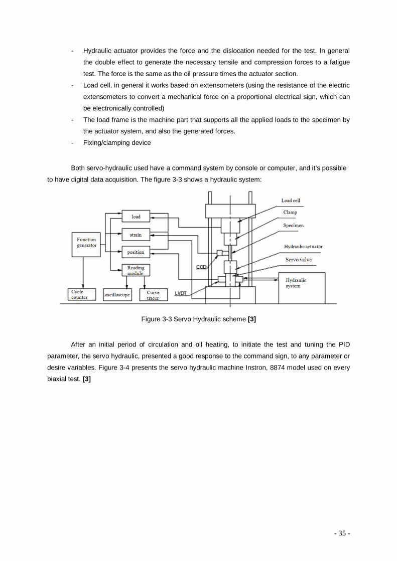
- 35 -
- Hydraulic actuator provides the force and the dislocation needed for the test. In general
the double effect to generate the necessary tensile and compression forces to a fatigue
test. The force is the same as the oil pressure times the actuator section.
- Load cell, in general it works based on extensometers (using the resistance of the electric
extensometers to convert a mechanical force on a proportional electrical sign, which can
be electronically controlled)
- The load frame is the machine part that supports all the applied loads to the specimen by
the actuator system, and also the generated forces.
- Fixing/clamping device
Both servo-hydraulic used have a command system by console or computer, and it’s possible
to have digital data acquisition. The figure 3-3 shows a hydraulic system:
Figure 3-3 Servo Hydraulic scheme [3]
After an initial period of circulation and oil heating, to initiate the test and tuning the PID
parameter, the servo hydraulic, presented a good response to the command sign, to any parameter or
desire variables. Figure 3-4 presents the servo hydraulic machine Instron, 8874 model used on every
biaxial test. [3]
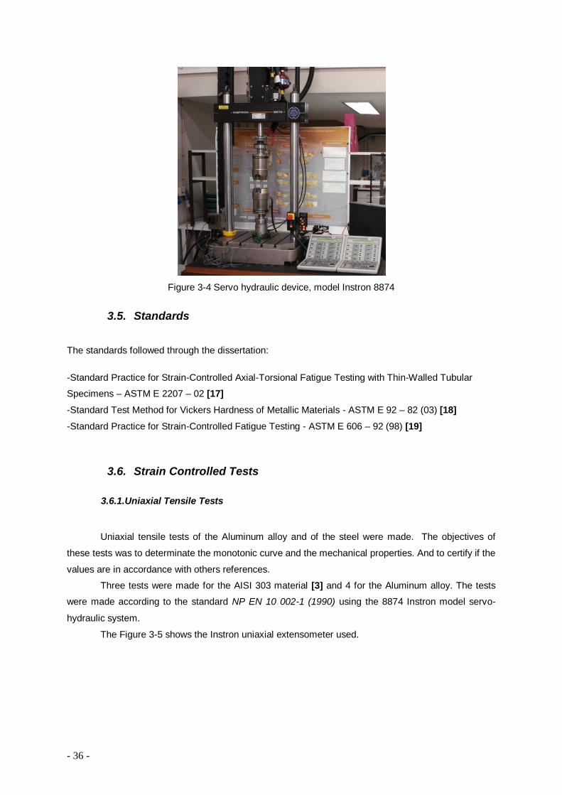
- 36 -
Figure 3-4 Servo hydraulic device, model Instron 8874
3.5. Standards
The standards followed through the dissertation:
-Standard Practice for Strain-Controlled Axial-Torsional Fatigue Testing with Thin-Walled Tubular
Specimens – ASTM E 2207 – 02 [17] -Standard Test Method for Vickers Hardness of Metallic Materials - ASTM E 92 – 82 (03) [18] -Standard Practice for Strain-Controlled Fatigue Testing - ASTM E 606 – 92 (98) [19]
3.6. Strain Controlled Tests
3.6.1. Uniaxial Tensile Tests
Uniaxial tensile tests of the Aluminum alloy and of the steel were made. The objectives of
these tests was to determinate the monotonic curve and the mechanical properties. And to certify if the
values are in accordance with others references.
Three tests were made for the AISI 303 material [3] and 4 for the Aluminum alloy. The tests
were made according to the standard NP EN 10 002-1 (1990) using the 8874 Instron model servo-
hydraulic system.
The Figure 3-5 shows the Instron uniaxial extensometer used.
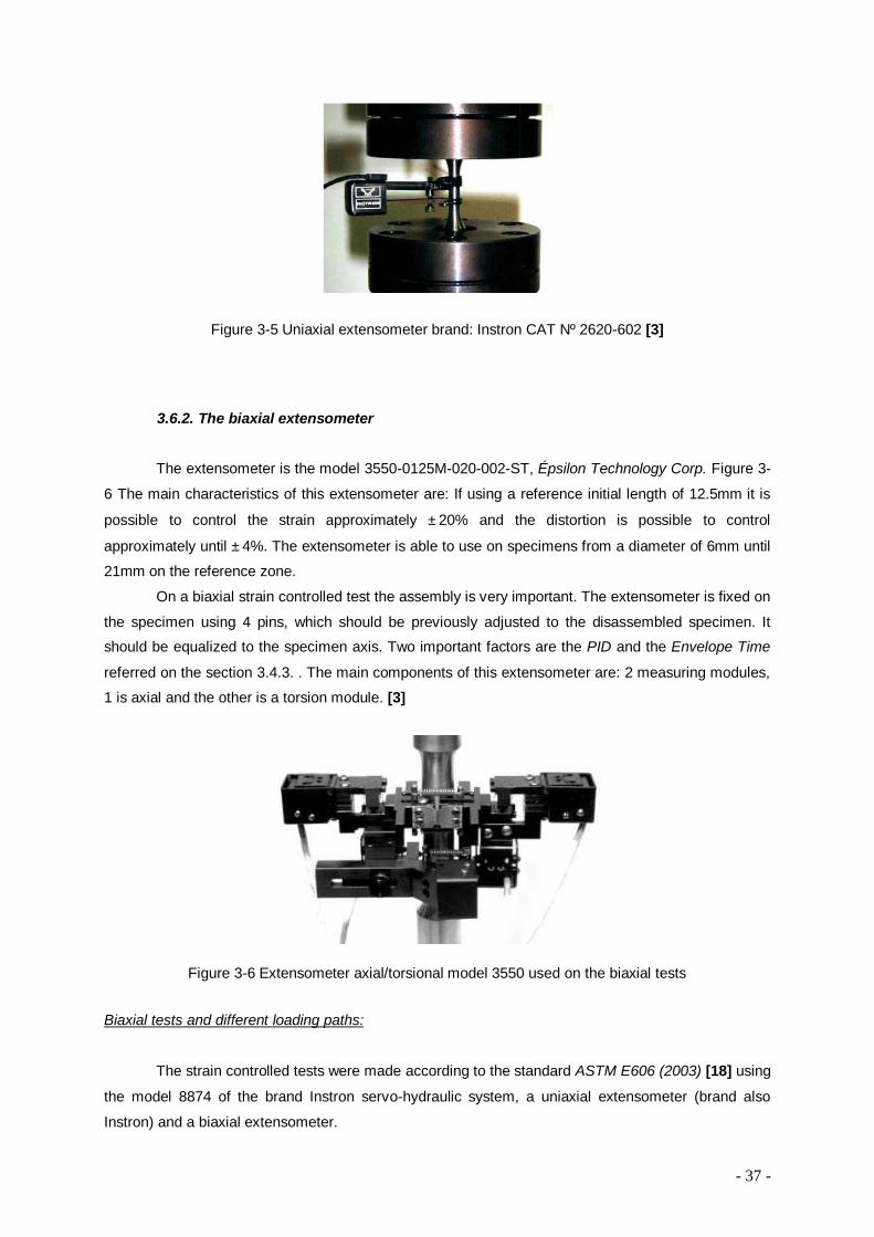
- 37 -
Figure 3-5 Uniaxial extensometer brand: Instron CAT Nº 2620-602 [3]
3.6.2. The biaxial extensometer
The extensometer is the model 3550-0125M-020-002-ST, Épsilon Technology Corp. Figure 3-
6 The main characteristics of this extensometer are: If using a reference initial length of 12.5mm it is
possible to control the strain approximately ±20% and the distortion is possible to control
approximately until ±4%. The extensometer is able to use on specimens from a diameter of 6mm until
21mm on the reference zone.
On a biaxial strain controlled test the assembly is very important. The extensometer is fixed on
the specimen using 4 pins, which should be previously adjusted to the disassembled specimen. It
should be equalized to the specimen axis. Two important factors are the PID and the Envelope Time
referred on the section 3.4.3. . The main components of this extensometer are: 2 measuring modules,
1 is axial and the other is a torsion module. [3]
Figure 3-6 Extensometer axial/torsional model 3550 used on the biaxial tests Biaxial tests and different loading paths:
The strain controlled tests were made according to the standard ASTM E606 (2003) [18] using
the model 8874 of the brand Instron servo-hydraulic system, a uniaxial extensometer (brand also
Instron) and a biaxial extensometer.
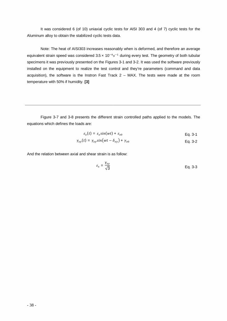
- 38 -
It was considered 6 (of 10) uniaxial cyclic tests for AISI 303 and 4 (of 7) cyclic tests for the
Aluminum alloy to obtain the stabilized cyclic tests data.
Note: The heat of AISI303 increases reasonably when is deformed, and therefore an average
equivalent strain speed was considered 3.5 × 10 푠 during every test. The geometry of both tubular
specimens it was previously presented on the Figures 3-1 and 3-2. It was used the software previously
installed on the equipment to realize the test control and they’re parameters (command and data
acquisition), the software is the Instron Fast Track 2 – MAX. The tests were made at the room
temperature with 50% if humidity. [3]
Figure 3-7 and 3-8 presents the different strain controlled paths applied to the models. The
equations which defines the loads are:
And the relation between axial and shear strain is as follow:
휀 (푡) = 휀 푠푖푛(푤푡) + 휀 Eq. 3-1 훾 (푡) = 훾 푠푖푛 푤푡 − 훿 + 훾 Eq. 3-2
휀 =훾√3
Eq. 3-3
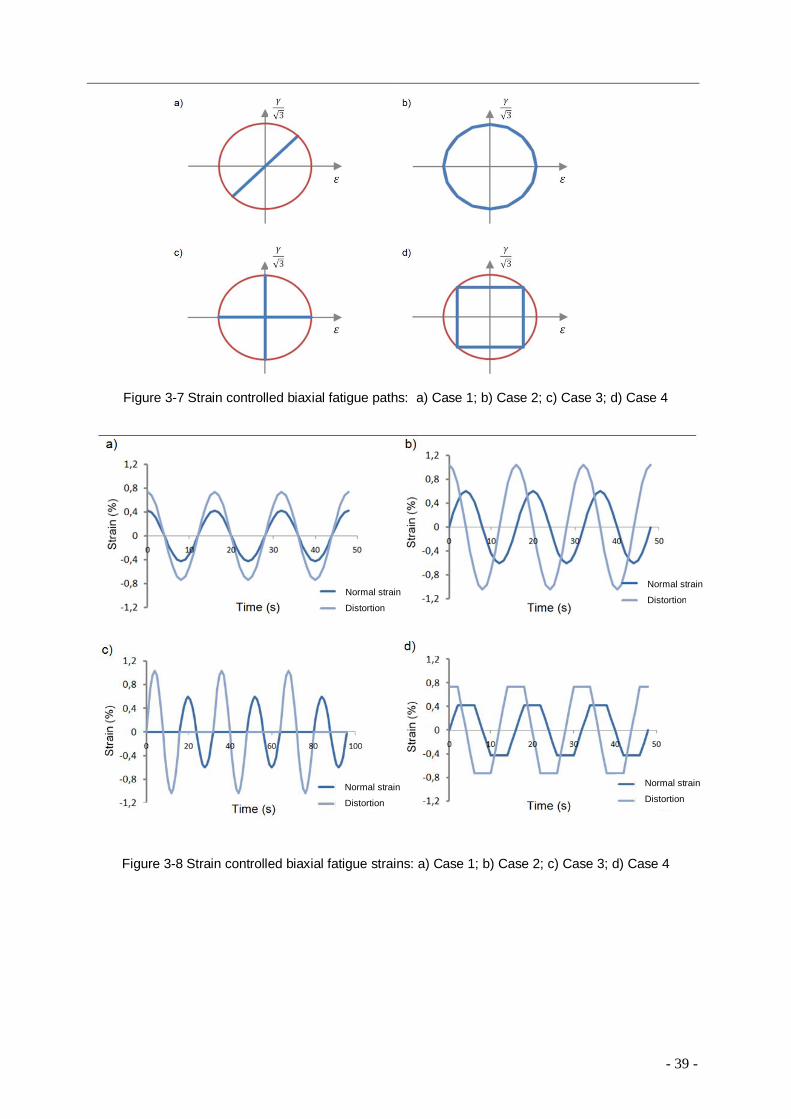
- 39 -
Figure 3-7 Strain controlled biaxial fatigue paths: a) Case 1; b) Case 2; c) Case 3; d) Case 4
Figure 3-8 Strain controlled biaxial fatigue strains: a) Case 1; b) Case 2; c) Case 3; d) Case 4
Normal strain
Distortion Normal strain
Distortion
Normal strain
Distortion
Normal strain
Distortion

- 40 -
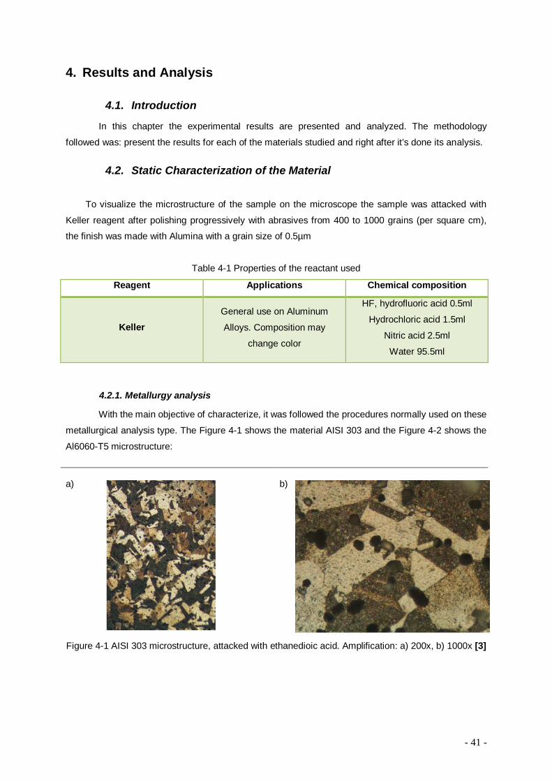
- 41 -
4. Results and Analysis
4.1. Introduction
In this chapter the experimental results are presented and analyzed. The methodology
followed was: present the results for each of the materials studied and right after it’s done its analysis.
4.2. Static Characterization of the Material
To visualize the microstructure of the sample on the microscope the sample was attacked with
Keller reagent after polishing progressively with abrasives from 400 to 1000 grains (per square cm),
the finish was made with Alumina with a grain size of 0.5µm
Table 4-1 Properties of the reactant used
4.2.1. Metallurgy analysis
With the main objective of characterize, it was followed the procedures normally used on these
metallurgical analysis type. The Figure 4-1 shows the material AISI 303 and the Figure 4-2 shows the
Al6060-T5 microstructure:
Figure 4-1 AISI 303 microstructure, attacked with ethanedioic acid. Amplification: a) 200x, b) 1000x [3]
Reagent Applications Chemical composition
Keller General use on Aluminum
Alloys. Composition may
change color
HF, hydrofluoric acid 0.5ml
Hydrochloric acid 1.5ml
Nitric acid 2.5ml
Water 95.5ml
a)
b)
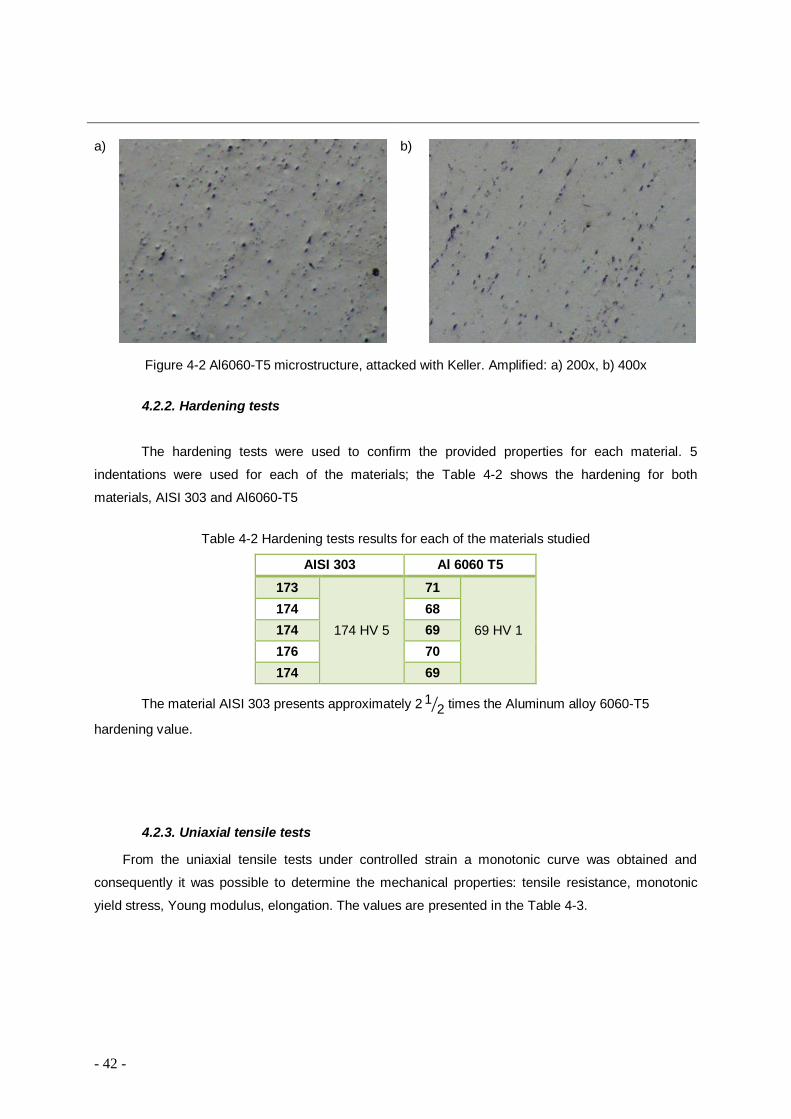
- 42 -
Figure 4-2 Al6060-T5 microstructure, attacked with Keller. Amplified: a) 200x, b) 400x
4.2.2. Hardening tests
The hardening tests were used to confirm the provided properties for each material. 5
indentations were used for each of the materials; the Table 4-2 shows the hardening for both
materials, AISI 303 and Al6060-T5
Table 4-2 Hardening tests results for each of the materials studied
The material AISI 303 presents approximately 2 1
2 times the Aluminum alloy 6060-T5
hardening value.
4.2.3. Uniaxial tensile tests
From the uniaxial tensile tests under controlled strain a monotonic curve was obtained and
consequently it was possible to determine the mechanical properties: tensile resistance, monotonic
yield stress, Young modulus, elongation. The values are presented in the Table 4-3.
a)
b)
AISI 303 Al 6060 T5 173
174 HV 5
71
69 HV 1 174 68 174 69 176 70 174 69

- 43 -
Table 4-3 Monotonic and cyclic mechanical properties of the materials studied Al 6060 T5 AISI 303
Tensile strength 푆 (MPa) 216 625 Yield strength 푅 . %, (MPa) 197 --- Yield strength 푅 (MPa) --- 330
Elongation A (%) 8 58 Young’s modulus 퐸(GPa) 79 178
Cyclic Yield strength 푅 . %, cyclic (MPa) 187 310 Strength coefficient 푘 (MPa) 503 2450
Strain hardening exponent 푛′ 0.156 0.35 Fatigue strength coefficient 휎 (MPa) 376.5 534 Fatigue strength exponent 푏 -0.084 -0.07 Fatigue ductility coefficient εf´ 0.157 0.052 Fatigue ductility exponent 푐 -0.537 -0.292
4.3. Uniaxial and biaxial tests under controlled strain
The uniaxial tests were made under strain controlled, tensile/compression, for 푅 = −1.
The biaxial tests were made for 4 different paths of multiaxial loading, one proportional and
three nonproportional cases.
Uniaxial cyclic tests were made, tension/compression.
Figures 4-3 shows the Shear stress-normal stress graphics for the 4 cases of the Aluminum
alloy under an equivalent strain of 0.25%.
Figures 4-4 shows the results for an equivalent strain of 0.60% to the case 1.
Figures 4-5 shows the results for an equivalent strain of 0.60% to the case 2.
Figures 4-6 shows the results for an equivalent strain of 0.60% to the case 3.
Figures 4-7 shows the results for an equivalent strain of 0.60% to the case 4.
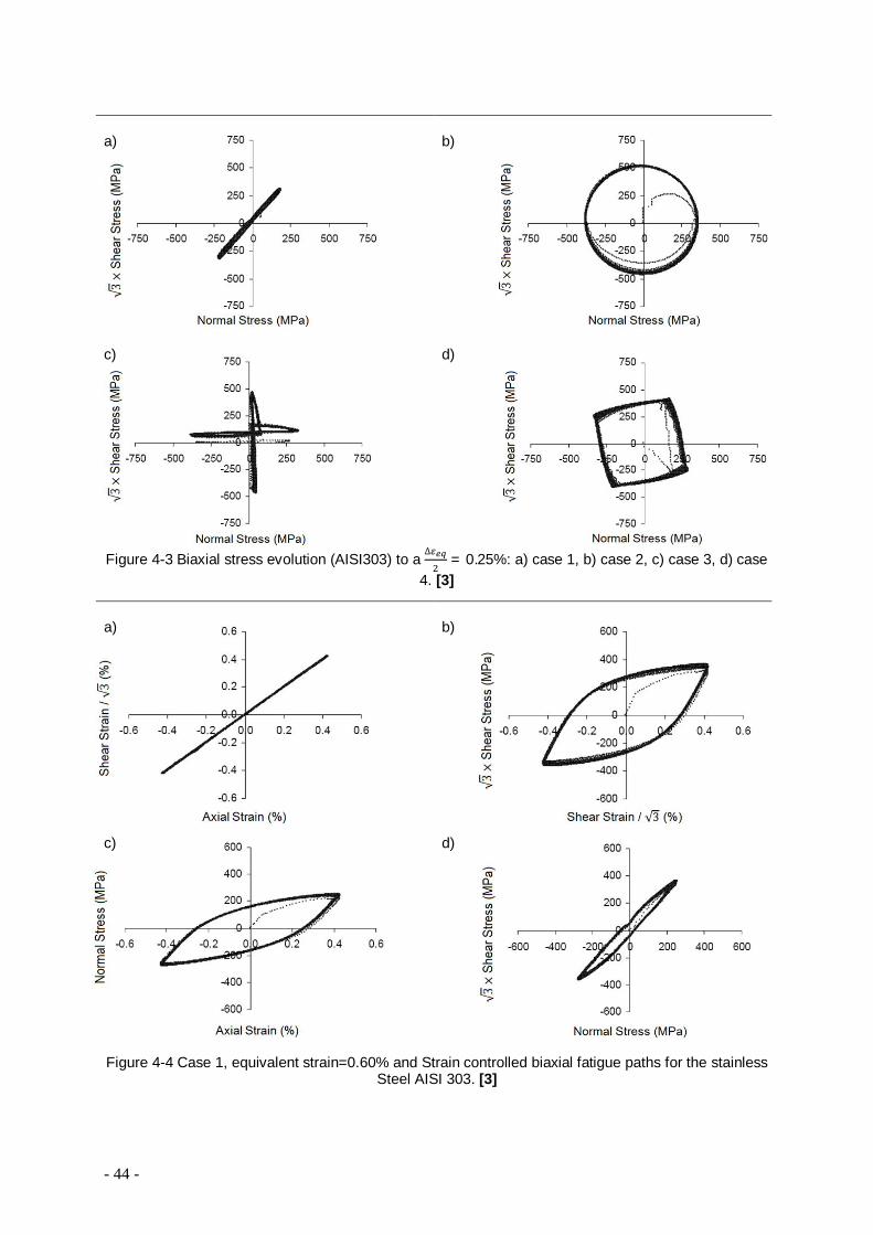
- 44 -
Figure 4-3 Biaxial stress evolution (AISI303) to a ∆ = 0.25%: a) case 1, b) case 2, c) case 3, d) case
4. [3]
Figure 4-4 Case 1, equivalent strain=0.60% and Strain controlled biaxial fatigue paths for the stainless Steel AISI 303. [3]
a)
b)
c)
d)
a)
b)
c)
d)
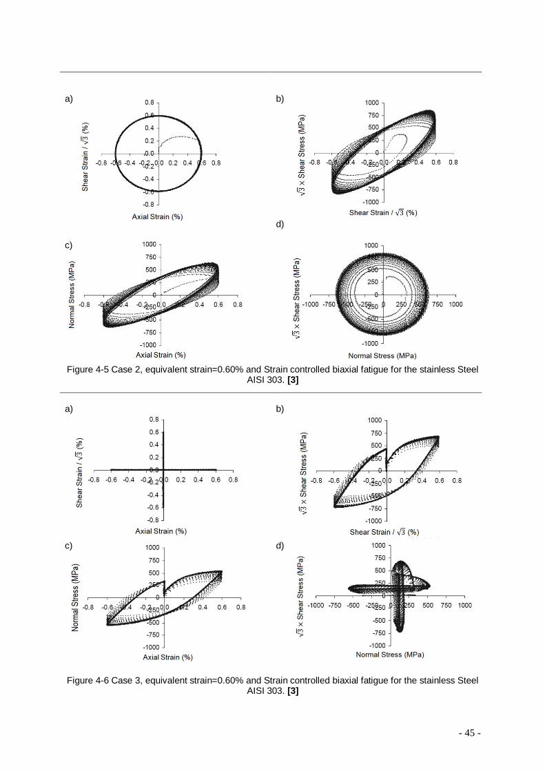
- 45 -
Figure 4-5 Case 2, equivalent strain=0.60% and Strain controlled biaxial fatigue for the stainless Steel AISI 303. [3]
Figure 4-6 Case 3, equivalent strain=0.60% and Strain controlled biaxial fatigue for the stainless Steel
AISI 303. [3]
a)
b)
c)
d)
a)
b)
c)
d)

- 46 -
Figure 4-7 Case 4, equivalent strain=0.60% and Strain controlled biaxial fatigue for the stainless Steel
AISI 303. [3]
Table 4-4 summarize the stress and equivalent strain amplitudes for all cases of the stainless Steel.
Table 4-4 Summary of obtained values to the proportional and nonproportional cases for the stainless
Steel
AISI 303 ∆흈ퟐ
∆휺풆풒ퟐ
N Cycles
Ref. Specimen
P Torsion
378 0,25 1000 IT2 463 0,60 1000 IT11
Case1 331 0,25 1000 IT4 420 0,60 1000 IT12
NP
Case2 491 0,25 1000 IT6 839 0,60 255 IT8
Case3 450 0,25 1000 IT9 755 0,60 80 IT10
Case4 414 0,25 1000 IT7 746 0,60 165 IT5
a)
b)
c)
d)
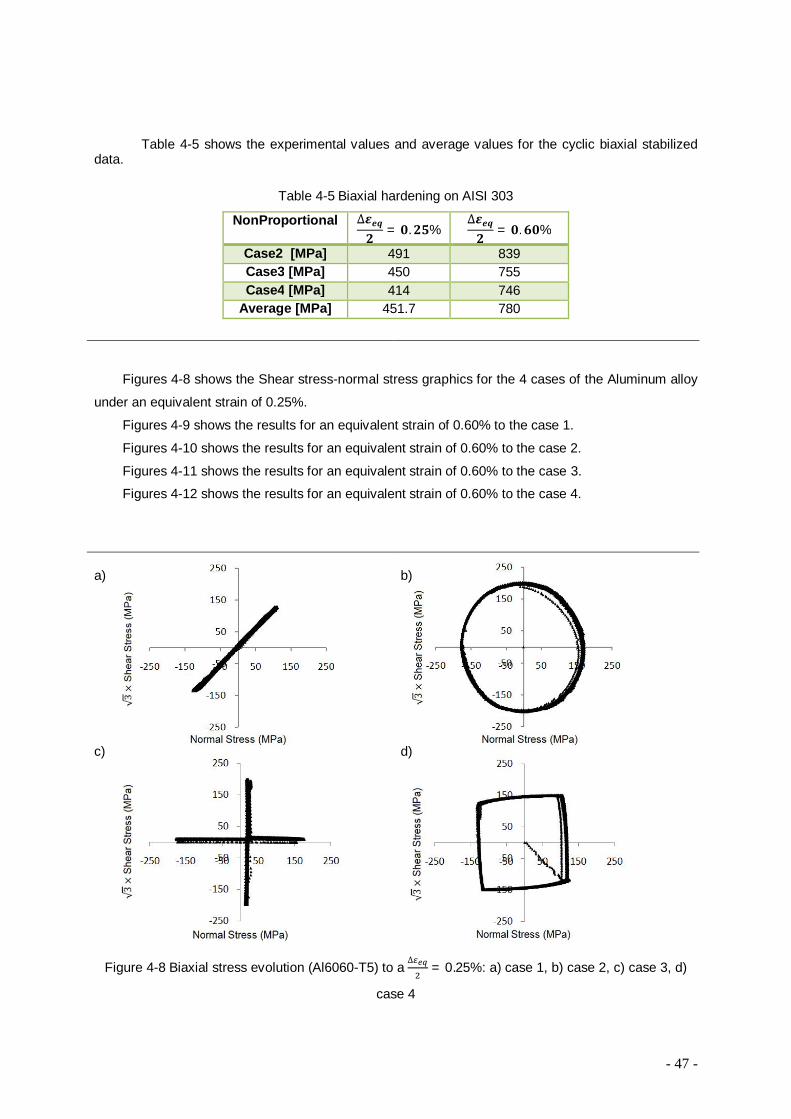
- 47 -
Table 4-5 shows the experimental values and average values for the cyclic biaxial stabilized data.
Table 4-5 Biaxial hardening on AISI 303
NonProportional ∆휺풆풒ퟐ = ퟎ.ퟐퟓ%
∆휺풆풒ퟐ = ퟎ.ퟔퟎ%
Case2 [MPa] 491 839 Case3 [MPa] 450 755 Case4 [MPa] 414 746
Average [MPa] 451.7 780
Figures 4-8 shows the Shear stress-normal stress graphics for the 4 cases of the Aluminum alloy
under an equivalent strain of 0.25%.
Figures 4-9 shows the results for an equivalent strain of 0.60% to the case 1.
Figures 4-10 shows the results for an equivalent strain of 0.60% to the case 2.
Figures 4-11 shows the results for an equivalent strain of 0.60% to the case 3.
Figures 4-12 shows the results for an equivalent strain of 0.60% to the case 4.
Figure 4-8 Biaxial stress evolution (Al6060-T5) to a ∆ = 0.25%: a) case 1, b) case 2, c) case 3, d)
case 4
a)
b)
c) d)
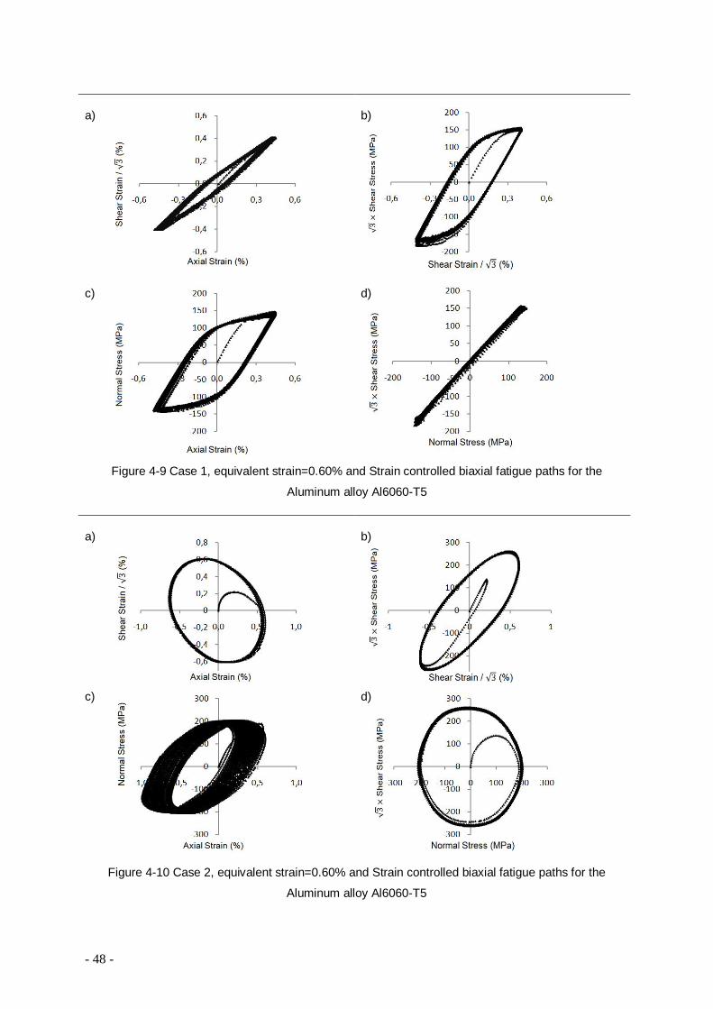
- 48 -
Figure 4-9 Case 1, equivalent strain=0.60% and Strain controlled biaxial fatigue paths for the
Aluminum alloy Al6060-T5
Figure 4-10 Case 2, equivalent strain=0.60% and Strain controlled biaxial fatigue paths for the
Aluminum alloy Al6060-T5
a)
b)
c) d)
a)
b)
c) d)

- 49 -
Figure 4-11 Case 3, equivalent strain=0.60% and Strain controlled biaxial fatigue for the Aluminum
alloy Al6060-T5
Figure 4-12 Case 3, equivalent strain=0.60% and Strain controlled biaxial fatigue paths for the
Aluminum alloy Al6060-T5
a)
b)
c) d)
a)
b)
c) d)
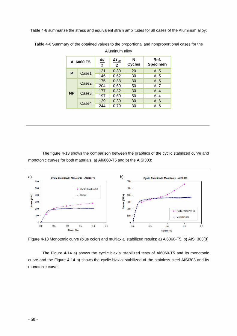
- 50 -
Table 4-6 summarize the stress and equivalent strain amplitudes for all cases of the Aluminum alloy:
Table 4-6 Summary of the obtained values to the proportional and nonproportional cases for the
Aluminum alloy
The figure 4-13 shows the comparison between the graphics of the cyclic stabilized curve and
monotonic curves for both materials, a) Al6060-T5 and b) the AISI303:
Figure 4-13 Monotonic curve (blue color) and multiaxial stabilized results: a) Al6060-T5, b) AISI 303[3]
The Figure 4-14 a) shows the cyclic biaxial stabilized tests of Al6060-T5 and its monotonic
curve and the Figure 4-14 b) shows the cyclic biaxial stabilized of the stainless steel AISI303 and its
monotonic curve:
Al 6060 T5 ∆흈ퟐ
∆휺풆풒ퟐ
N Cycles
Ref. Specimen
P Case1 121 0,30 20 Al 5 146 0,62 30 Al 5
NP
Case2 175 0,33 30 Al 5 204 0,60 50 Al 7
Case3 177 0,32 30 Al 4 197 0,60 50 Al 4
Case4 129 0,30 30 Al 6 244 0,70 30 Al 6
a)
b)
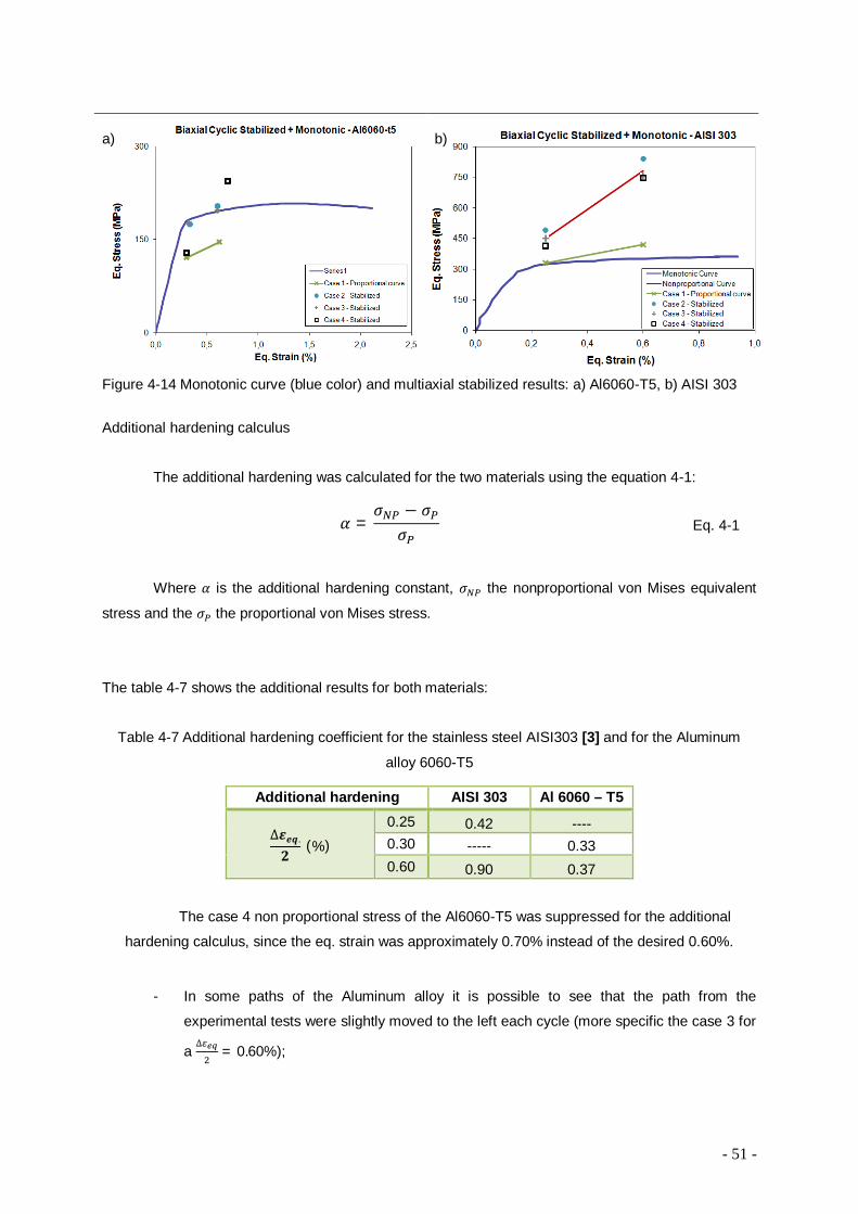
- 51 -
Figure 4-14 Monotonic curve (blue color) and multiaxial stabilized results: a) Al6060-T5, b) AISI 303 Additional hardening calculus
The additional hardening was calculated for the two materials using the equation 4-1:
Where 훼 is the additional hardening constant, 휎 the nonproportional von Mises equivalent
stress and the 휎 the proportional von Mises stress.
The table 4-7 shows the additional results for both materials:
Table 4-7 Additional hardening coefficient for the stainless steel AISI303 [3] and for the Aluminum
alloy 6060-T5
The case 4 non proportional stress of the Al6060-T5 was suppressed for the additional
hardening calculus, since the eq. strain was approximately 0.70% instead of the desired 0.60%.
- In some paths of the Aluminum alloy it is possible to see that the path from the
experimental tests were slightly moved to the left each cycle (more specific the case 3 for
a ∆ = 0.60%);
a)
b)
훼 =휎 − 휎
휎 Eq. 4-1
Additional hardening AISI 303 Al 6060 – T5
∆휺풆풒.
ퟐ (%) 0.25 0.42 ---- 0.30 ----- 0.33 0.60 0.90 0.37

- 52 -
- The proportional curve for the Aluminum alloy is nearly 40 MPa lower than the monotonic
curve;
- The case 2 for the Aluminum alloy is approximately the same as the monotonic curve.
- The experimental results for the Aluminum alloy should have been made with an
equivalent strain higher than 0.60%, as a result no “nonproportional curve” was used
further on F.E.M.
- Between the cyclic stabilized curve and the monotonic curve for both materials there is a
possibility to occur a steady state;
- For the AISI 303 stainless steel higher stabilized values are reached for the
nonproportional cases;
- Hysteresis loops results of type AISI 303 steel under controlled strain with proportional
and nonproportional loads. Test on from the results analysis it was observed that to the
same strain amplitude the nonproportional tests have stress amplitude almost twice the
proportional test. Although both load paths have the same shear strain amplitude the
fatigue life to the out-of-phase load is about twenty times less when compared with the
proportional load. With the hysteresis loops it’s also possible to see that an out-of-phase
load has a plastic strain less that the proportional case, this means that the plastic strain
only by itself is not responsible to the fatigue damage; [3]
- The Aluminum alloy presents a lower additional hardening coefficient.
- 53 -
5. Finite Element Method Study
5.1. Introduction
The finite element method was developed on 1956 by Turner, Clough, Martin and Topp. It is a
numerical technique for finding approximate solutions of partial differential equations as well as of
integral equations. Today this method is a technique with a wide application field e.g. heat
transmission, structural optimization and analysis and fluid mechanics. On the particular case of
analysis and structural the FEM is a powerful and versatile technique used on mechanical design and
analysis. [3] Fatigue failure on mechanical components can be described as a local phenomenon, where
occurs cyclic evolution of the stresses, deformations and distribution on a certain critical volume of
material. On a fatigue loading cyclic plastic deformation will occur and consequently cracks nucleation,
the mechanical resistance of the material will decrease. And because of that the simulation of the
stress evolution and cyclic deformation and its distribution plays a fundamental role on fatigue life
prediction of mechanical components.
Modeling the cyclic behavior of a material under elastoplastic multiaxial deformations it is
fundamental to predict the fatigue life of the components, using the criterions that define the multiaxial
fatigue. A usual procedure on fatigue design uses the study via the local stress time history to detect
critical zones, under a specific loading cycles, and prediction of cracks by the application of an
appropriate multiaxial fatigue criterion. [3,17]
The numerical study it is focused on the stress-strain cyclic deformation under a biaxial
loading, proportional or nonproportional. When solving partial differential equations, the primary
challenge is to create an equation that approximates the equation to be studied, but is numerically
stable, meaning that errors in the input data and intermediate calculations do not accumulate and
cause the resulting output to be meaningless. There are many ways of doing this, all with advantages
and disadvantages. The Finite Element Method is a good choice for solving partial differential
equations over complex domains (like cars and oil pipelines), when the domain changes (as during a
solid state reaction with a moving boundary), when the desired precision varies over the entire
domain, or when the solution lacks smoothness. For instance, in simulating the weather pattern on
Earth, it is more important to have accurate predictions over land than over the wide-open sea, a
demand that is achievable using the finite element method. [20]
Modeling the mechanical behavior of a material under multiaxial elastoplastic strain becomes
fundamental to predict the fatigue life of the components, using the multiaxial fatigue criteria. A usual
procedure when designing to long life is to initiate the study using the FEM on the calculation of the
elastic local stress-time history, finding that way the critical zones of the components. After the
evaluation of these critical zones under a specific a load cycle number cracks initiation can be
predicted with an application of a proper criterion.
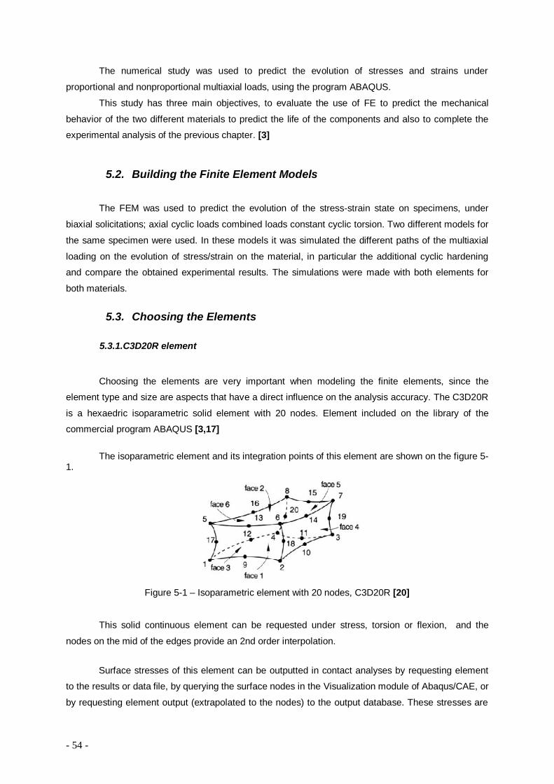
- 54 -
The numerical study was used to predict the evolution of stresses and strains under
proportional and nonproportional multiaxial loads, using the program ABAQUS.
This study has three main objectives, to evaluate the use of FE to predict the mechanical
behavior of the two different materials to predict the life of the components and also to complete the
experimental analysis of the previous chapter. [3]
5.2. Building the Finite Element Models
The FEM was used to predict the evolution of the stress-strain state on specimens, under
biaxial solicitations; axial cyclic loads combined loads constant cyclic torsion. Two different models for
the same specimen were used. In these models it was simulated the different paths of the multiaxial
loading on the evolution of stress/strain on the material, in particular the additional cyclic hardening
and compare the obtained experimental results. The simulations were made with both elements for
both materials.
5.3. Choosing the Elements
5.3.1. C3D20R element
Choosing the elements are very important when modeling the finite elements, since the
element type and size are aspects that have a direct influence on the analysis accuracy. The C3D20R
is a hexaedric isoparametric solid element with 20 nodes. Element included on the library of the
commercial program ABAQUS [3,17]
The isoparametric element and its integration points of this element are shown on the figure 5-
1.
Figure 5-1 – Isoparametric element with 20 nodes, C3D20R [20]
This solid continuous element can be requested under stress, torsion or flexion, and the
nodes on the mid of the edges provide an 2nd order interpolation.
Surface stresses of this element can be outputted in contact analyses by requesting element
to the results or data file, by querying the surface nodes in the Visualization module of Abaqus/CAE, or
by requesting element output (extrapolated to the nodes) to the output database. These stresses are

- 55 -
extrapolated from the integration points. The surface can be coated with very thin membrane elements
that have stiffness comparable to the underlying material. The stresses on these membrane elements
will then reflect the surface stress more accurately. [20]
5.3.2. Pipe31 element
Pipe31 was the element used in the new model, which is simpler in both numerical and
modeling way, this element, is an Timoshenko (shear flexible) beam, which allows transverse shear
strain for beams made from uniform material.
The shear flexible beam theory can provide useful results for cross-sectional dimensions up to
1/8 of typical axial distances or the wavelength of the highest natural mode that contributes
significantly to the response. Beyond this ratio the approximations that allow the member's behavior to
be described solely as a function of axial position no longer provide adequate accuracy.
Abaqus assumes that the transverse shear behavior of Timoshenko beams is linear elastic
with a fixed modulus and, thus, independent of the response of the beam section to axial stretch and
bending. [20]
These beams can be subjected to large axial strains. The axial strains due to torsion are
assumed to be small. In combined axial-torsion loading, torsional shear strains are calculated
accurately only when the axial strain is not large.
The element PIPE31, use linear interpolation. This element is well suited for cases involving
contact, such as the laying of a pipeline in a trench or on the seabed or the contact between a drill
string and a well hole, and for dynamic versions of similar problems. [20]
5.4. Definition and Mesh Dimension
The used C3D20R mesh was carefully chosen, to diminish undesired distortions on the mesh
elements, which could lead to serious errors, such as: simulation crashes or the solution didn’t
converge to any result. The model is axisymmetric and the mesh generation was semi-automatic.
The mesh of the pipe31 model, is very simple, since each element already represents a
partition of a tube, the number of elements used was decided to be five, since the results were
considered basically the same for every element.
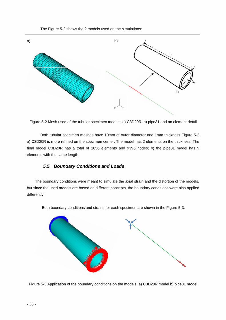
- 56 -
The Figure 5-2 shows the 2 models used on the simulations:
Figure 5-2 Mesh used of the tubular specimen models: a) C3D20R, b) pipe31 and an element detail
Both tubular specimen meshes have 10mm of outer diameter and 1mm thickness Figure 5-2
a) C3D20R is more refined on the specimen center. The model has 2 elements on the thickness. The
final model C3D20R has a total of 1656 elements and 9396 nodes; b) the pipe31 model has 5
elements with the same length.
5.5. Boundary Conditions and Loads
The boundary conditions were meant to simulate the axial strain and the distortion of the models,
but since the used models are based on different concepts, the boundary conditions were also applied
differently:
Both boundary conditions and strains for each specimen are shown in the Figure 5-3:
Figure 5-3 Application of the boundary conditions on the models: a) C3D20R model b) pipe31 model
a)
b)

- 57 -
After testing different ways to simulate the distortion, the final approach used is the shown on
Figure 5-3 a), were the stress concentrations were minimum, this models uses 4 dislocations in 5
nodes each out of phased by 90 degrees so the simulation of the distortion was possible.
The paths on ABAQUS were defined with a variation of the AMPLITUDE command, with this
command is possible to produce the form of the desire signal, with a time change wave varying
between -1 and 1, and then multiply this wave with the corresponding equivalent strain to produce the
final strain path.
On both tubular specimens were simulated 4 cases: the case 1 is a proportional case, the
case 2 follows a circular path, the case 3 forms a cross and at last the case 4 a square. The biaxial
loads were simulated under controlled strain, which means the application of alternated combined
axial cyclic strain with alternated cyclic distortion for all different paths.
The loads are applied on the specimen end nodes and it is also defined the dislocations and
distortion of the models.
Two different equivalent strain amplitude were applied on both materials AISI303 and Al6060-
T5 (∆ = 0.25% and
∆ = 0.60%).
The Figure 5-4 shows the critical elements which behavior was analyzed for each model:
Figure 5-4 Critical elements of both models: a) Element 259 - C3D20R model b) Element 3 - pipe31 model

- 58 -
5.6. Hardening law
As mentioned on State of Art, the hardening law used on the finite elements has a significant
influence on the obtained results.
It was decided to compare all the hardening laws, isotropic, kinematic and the combination of
isotropic and kinematic (combined).
As described before (chapter II) the hardening law used to simulate the finite elements has a
significant influence on the results. And therefore it was used the following hardening laws: isotropic
with monotonic data, kinematic with linear data, combined with monotonic cyclic hardening and cyclic
stabilized uniaxial data, and for the AISI303 material it was also used the combined hardening with
experimental stabilized biaxial data and the monotonic cyclic hardening data.
The 29 simulations of the C3D20R element models simulations used about 50 hours of time
processor (105 minutes each simulation, maximum ~180 minutes), the 96 pipe31 model used about
176 minutes of time processor (110 seconds each simulation, maximum ~180 seconds).
Table 5-1 CPU usage with the different elements
Element Type Average CPU usage Computer characteristics
C3D20R ~70% AMD Sempron 2800+, 1GB
ram Pipe31 ~99%
The Abaqus output: stresses (S), strains (E), plastic strains (PE) and dislocations (U), these
were the outputs considered more relevant to this study.
5.7. Results
The following sections present the main F.E.M. results.
- The section 5.7.1. presents the paths used on pipe31 models for an equivalent strain of
0.25%.
- The section 5.7.2. presents the comparison between the pipe31 model and the C3D20R
model for an equivalent strain of 0.60%
- The section 5.7.3 presents the pipe31 results for the AISI303 under an equivalent strain
of 0.25% and an equivalent strain of 0.60% for all four cases
- The section 5.7.4. presents the pipe31 results for the Aluminum alloy 6060 age hardened
T5 with an equivalent strain of 0.60%
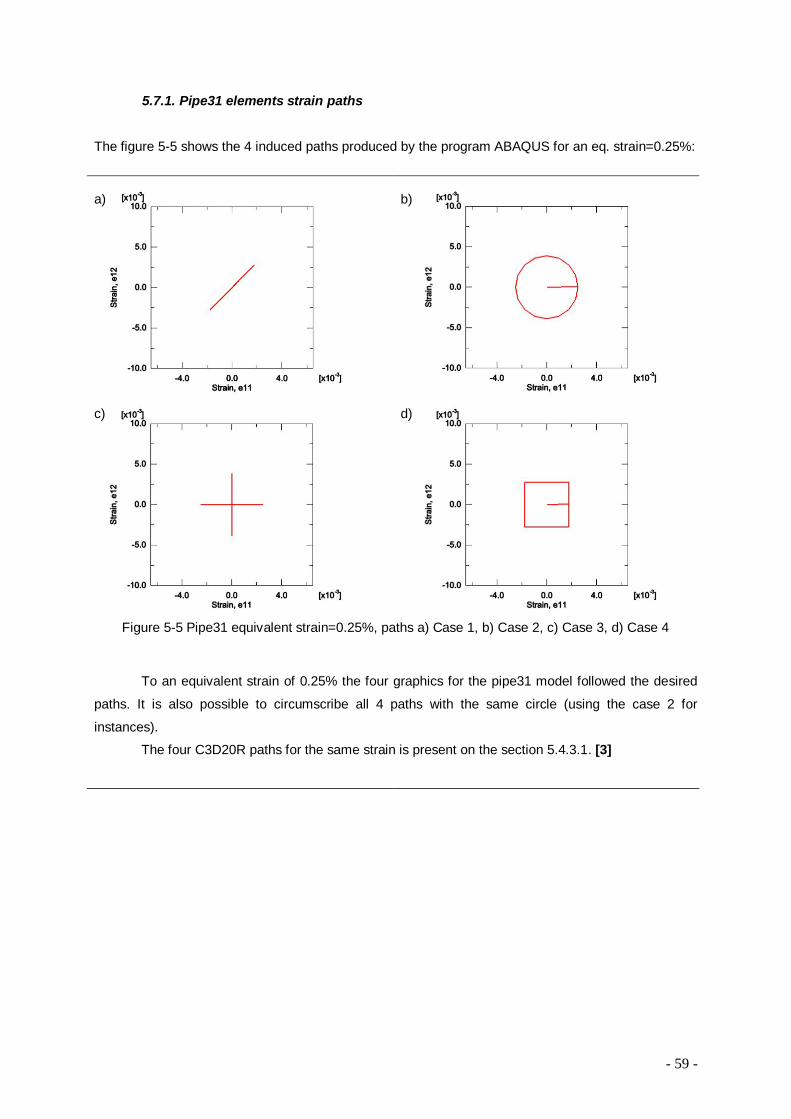
- 59 -
5.7.1. Pipe31 elements strain paths
The figure 5-5 shows the 4 induced paths produced by the program ABAQUS for an eq. strain=0.25%:
Figure 5-5 Pipe31 equivalent strain=0.25%, paths a) Case 1, b) Case 2, c) Case 3, d) Case 4
To an equivalent strain of 0.25% the four graphics for the pipe31 model followed the desired
paths. It is also possible to circumscribe all 4 paths with the same circle (using the case 2 for
instances).
The four C3D20R paths for the same strain is present on the section 5.4.3.1. [3]
a)
b)
c)
d)
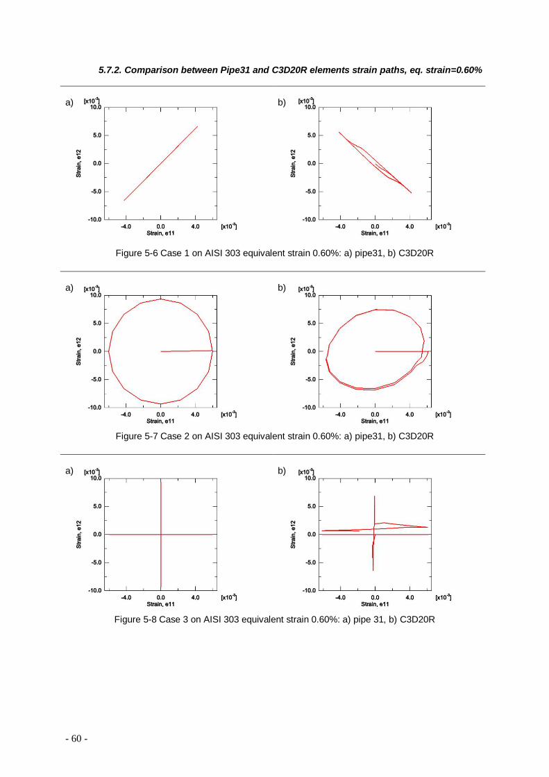
- 60 -
5.7.2. Comparison between Pipe31 and C3D20R elements strain paths, eq. strain=0.60%
Figure 5-6 Case 1 on AISI 303 equivalent strain 0.60%: a) pipe31, b) C3D20R
Figure 5-7 Case 2 on AISI 303 equivalent strain 0.60%: a) pipe31, b) C3D20R
Figure 5-8 Case 3 on AISI 303 equivalent strain 0.60%: a) pipe 31, b) C3D20R
a)
b)
a)
b)
a)
b)

- 61 -
Figure 5-9 Case 4 on AISI 303 equivalent strain 0.60%: a) pipe31, b) C3D20R
Since the distortion applied on the C3D20R does not follow the exact path, the resulting cases
are not exactly as predicted. More specifically:
The case 1, is not totally proportional, obviously because both axial strain and distortion are
not proportional, although the case is not proportional the values of axial strain and distortion reaches
approximately the maximum value; the case 2 does not follow a circular path although the axial strain
reaches is maximum desired value the distortion fails to reach its correspondent maximum value; the
same behavior of case 2 happens on both cases 3 and 4.
The C3D20R model presented a different path for each case to the Aluminum alloy, making
the same comparison using the pipe31 model this was not observed. This difference of C3D20R
models is probably due to the material properties, a difference that should not affect the strain path,
since the simulation is under controlled strain.
a)
b)

- 62 -
5.7.3. Pipe 31 Models AISI 303
Eq. Strain=0.25% - case 1
Figure 5-10 Case 1: Equivalent Strain=0.25%; Material=AISI 303; Element Type: Pipe31; Modeling properties: Kinematic Hardening - Linear data: a) Stress-Torsion evolution, b) Axial Stress-Strain
evolution
Figure 5-11 Case 1: Equivalent Strain=0.25%; Material=AISI 303; Element Type: Pipe31; Modeling properties: Combined Hardening – Stabilized; Cyclic hardening - monotonic data: a) Stress-Torsion
evolution, b) Axial Stress-Strain evolution
a)
b)
Figure 5-12 Case 1: Equivalent Strain=0.25%; Material=AISI 303; Element Type: Pipe31; Modeling properties: Combined Hardening, stabilized data, multiaxial hardening data: a) Stress-Torsion
evolution, b) Axial Stress-Strain evolution
a)
b)
a)
b)

- 63 -
Eq. Strain=0.25% - case 2
a)
b)
Figure 5-13 Case 2: Equivalent Strain=0.25%; Material=AISI 303; Element Type: Pipe31; Modeling properties: Kinematic Hardening - Linear data: a) Stress-Torsion evolution, b) Axial Stress-Strain
evolution
Figure 5-14 Case 2: Equivalent Strain=0.25%; Material=AISI 303; Element Type: Pipe31; Modeling properties: Combined Hardening – Stabilized; Cyclic hardening - monotonic data: a) Stress-Torsion
evolution, b) Axial Stress-Strain evolution
Figure 5-15 Case 2: Equivalent Strain=0.25%; Material=AISI 303; Element Type: Pipe31; Modeling properties: Combined Hardening, stabilized data, multiaxial hardening data: a) Stress-Torsion
evolution, b) Axial Stress-Strain evolution
a)
b)
a)
b)
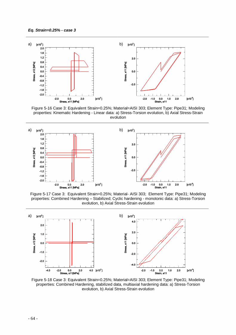
- 64 -
Eq. Strain=0.25% - case 3
Figure 5-16 Case 3: Equivalent Strain=0.25%; Material=AISI 303; Element Type: Pipe31; Modeling properties: Kinematic Hardening - Linear data: a) Stress-Torsion evolution, b) Axial Stress-Strain
evolution
Figure 5-17 Case 3: Equivalent Strain=0.25%; Material- AISI 303; Element Type: Pipe31; Modeling properties: Combined Hardening – Stabilized; Cyclic hardening - monotonic data: a) Stress-Torsion
evolution, b) Axial Stress-Strain evolution
Figure 5-18 Case 3: Equivalent Strain=0.25%; Material=AISI 303; Element Type: Pipe31; Modeling
properties: Combined Hardening, stabilized data, multiaxial hardening data: a) Stress-Torsion evolution, b) Axial Stress-Strain evolution
a)
b)
a)
b)
a)
b)

- 65 -
Eq. Strain=0.25% - case 4
Figure 5-19 Case 4: Equivalent Strain=0.25%; Material=AISI 303; Element Type: Pipe31; Modeling properties: Kinematic Hardening - Linear data: a) Stress-Torsion evolution, b) Axial Stress-Strain
evolution a)
b)
Figure 5-20 Case 4: Equivalent Strain=0.25%; Material=AISI 303; Element Type: Pipe31; Modeling properties: Combined Hardening – Stabilized; Cyclic hardening - monotonic data: a) Stress-Torsion
evolution, b) Axial Stress-Strain evolution
a)
b)
Figure 5-21 Case 4: Equivalent Strain=0.25%; Material=AISI 303; Element Type: Pipe31; Modeling properties: Combined Hardening, stabilized data, multiaxial hardening data: a) Stress-Torsion
evolution, b) Axial Stress-Strain evolution
a)
b)
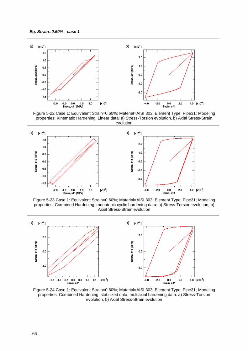
- 66 -
Eq. Strain=0.60% - case 1
Figure 5-22 Case 1: Equivalent Strain=0.60%; Material=AISI 303; Element Type: Pipe31; Modeling properties: Kinematic Hardening, Linear data: a) Stress-Torsion evolution, b) Axial Stress-Strain
evolution a)
b)
Figure 5-23 Case 1: Equivalent Strain=0.60%; Material=AISI 303; Element Type: Pipe31; Modeling properties: Combined Hardening, monotonic cyclic hardening data: a) Stress-Torsion evolution, b)
Axial Stress-Strain evolution
Figure 5-24 Case 1: Equivalent Strain=0.60%; Material=AISI 303; Element Type: Pipe31; Modeling properties: Combined Hardening, stabilized data, multiaxial hardening data: a) Stress-Torsion
evolution, b) Axial Stress-Strain evolution
a)
b)
a)
b)
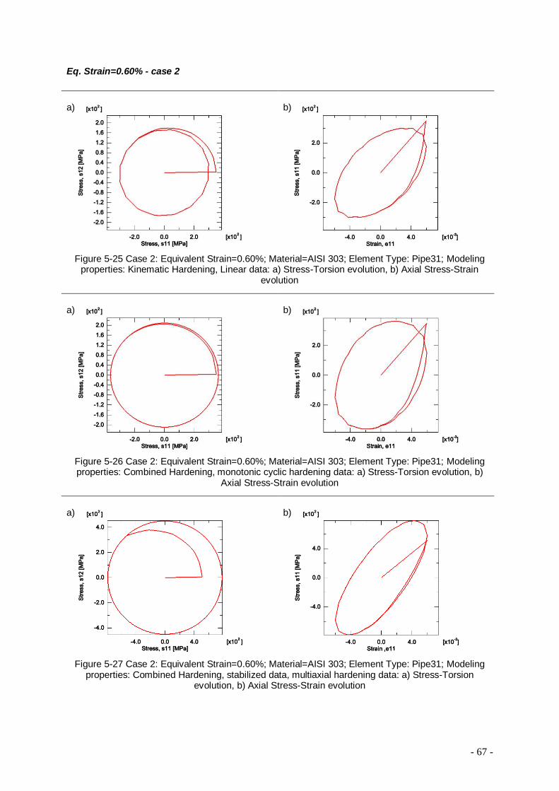
- 67 -
Eq. Strain=0.60% - case 2 a)
b)
Figure 5-25 Case 2: Equivalent Strain=0.60%; Material=AISI 303; Element Type: Pipe31; Modeling
properties: Kinematic Hardening, Linear data: a) Stress-Torsion evolution, b) Axial Stress-Strain evolution
Figure 5-26 Case 2: Equivalent Strain=0.60%; Material=AISI 303; Element Type: Pipe31; Modeling properties: Combined Hardening, monotonic cyclic hardening data: a) Stress-Torsion evolution, b)
Axial Stress-Strain evolution
Figure 5-27 Case 2: Equivalent Strain=0.60%; Material=AISI 303; Element Type: Pipe31; Modeling properties: Combined Hardening, stabilized data, multiaxial hardening data: a) Stress-Torsion
evolution, b) Axial Stress-Strain evolution
a)
b)
a)
b)
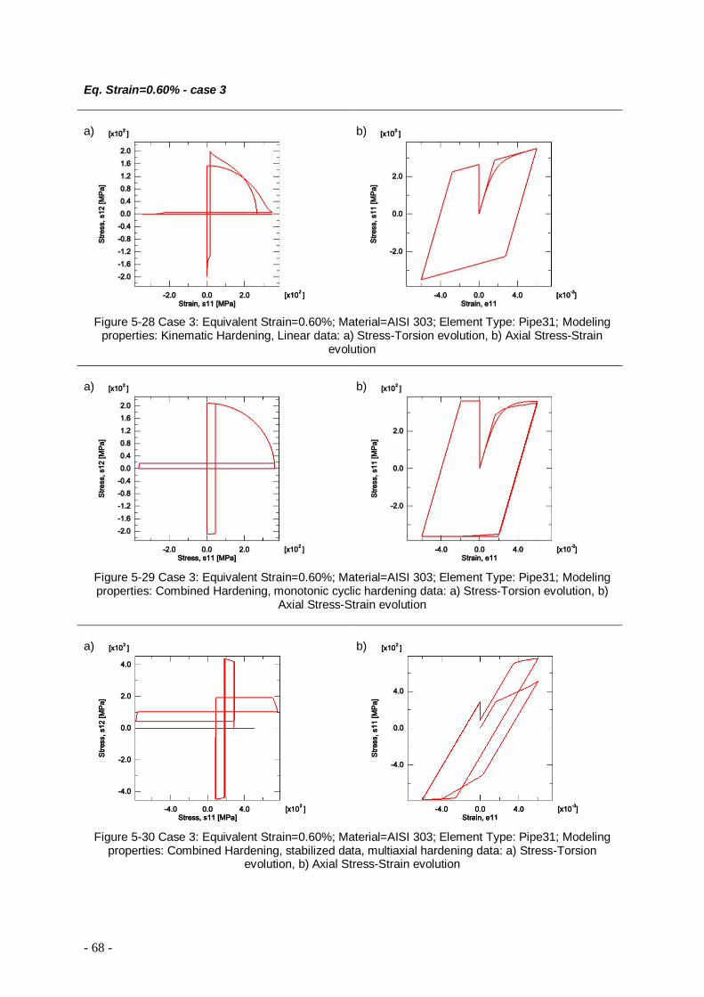
- 68 -
Eq. Strain=0.60% - case 3
Figure 5-28 Case 3: Equivalent Strain=0.60%; Material=AISI 303; Element Type: Pipe31; Modeling properties: Kinematic Hardening, Linear data: a) Stress-Torsion evolution, b) Axial Stress-Strain
evolution
Figure 5-29 Case 3: Equivalent Strain=0.60%; Material=AISI 303; Element Type: Pipe31; Modeling properties: Combined Hardening, monotonic cyclic hardening data: a) Stress-Torsion evolution, b)
Axial Stress-Strain evolution
a)
b)
Figure 5-30 Case 3: Equivalent Strain=0.60%; Material=AISI 303; Element Type: Pipe31; Modeling properties: Combined Hardening, stabilized data, multiaxial hardening data: a) Stress-Torsion
evolution, b) Axial Stress-Strain evolution
a)
b)
a)
b)
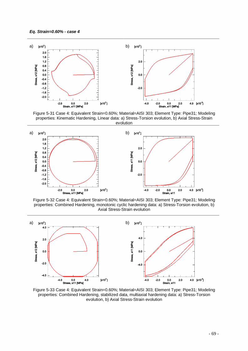
- 69 -
Eq. Strain=0.60% - case 4
Figure 5-31 Case 4: Equivalent Strain=0.60%; Material=AISI 303; Element Type: Pipe31; Modeling properties: Kinematic Hardening, Linear data: a) Stress-Torsion evolution, b) Axial Stress-Strain
evolution a)
b)
Figure 5-32 Case 4: Equivalent Strain=0.60%; Material=AISI 303; Element Type: Pipe31; Modeling properties: Combined Hardening, monotonic cyclic hardening data: a) Stress-Torsion evolution, b)
Axial Stress-Strain evolution
Figure 5-33 Case 4: Equivalent Strain=0.60%; Material=AISI 303; Element Type: Pipe31; Modeling properties: Combined Hardening, stabilized data, multiaxial hardening data: a) Stress-Torsion
evolution, b) Axial Stress-Strain evolution
a)
b)
a)
b)
- 70 -
Note: the combined hardening using multiaxial data on the cyclic hardening uses a different scale,
consequence of the large difference between the results of the models.
Equivalent strain=0.25%
- When using multiaxial hardening data there is no significant difference between the
maximum values. Behavior that can be explained by the low difference between the
values of the equivalent stress of the monotonic curve and the stabilized nonproportional
multiaxial curve;
- For these curves it is easier to analyze the hardening on the material, this behavior can be
explained by the smaller difference, between the values of plastic strain and the elastic
strain for this equivalent strain;
- Using the kinematic hardening law with linear data reveals to be less accurate than
Isotropic and Combined hardening, since this approximation neglects the behavior of the
material during the major part of the monotonic curve.
Equivalent strain=0.60%
- For the case 1, when using the multiaxial cyclic hardening data the results are slightly
above than the other 3 types of hardening;
- For the cases 2, 3 and 4 using multiaxial cyclic hardening data, the stress is roughly two
times the stress when using the other three types of hardening;
- Between the models: combined using monotonic data, kinematic and isotropic, the
differences between the shear stress-axial stress graphics are mainly due to the use of
linear data on the kinematic model, since is a less accurate model;
- Proportional case: The results using the multiaxial data is slightly above the other models,
this behavior can be explained by the fact that the proportional curve is very close to the
monotonic curve for this material;
- Nonproportional cases: using the multiaxial data for nonproportional cases is roughly 2
times more than the stress of the kinematic and monotonic combined data of the other
models, the behavior of the models can be explained by the values of the equivalent
stress for the equivalent strain of 0.60%;
- Only the case 3 model for an equivalent strain of 0.60% (the simulation using cyclic
multiaxial hardening data) stabilized before the end of the first cycle;
- To this equivalent strain the additional hardening is better shown on the case 2 and 4 for
the model using combined hardening with multiaxial hardening data.

- 71 -
5.7.4. Pipe 31 Models Al6060–T5 0.60%
Figure 5-34 Case 1: Equivalent Strain=0.60%; Material=Al6060-T5; Element Type: Pipe31; Modeling properties: Combined Hardening – Stabilized; Cyclic hardening - monotonic data a) Stress-Torsion
evolution, b) Axial Stress-Strain evolution a)
b)
Figure 5-35 Case 2: Equivalent Strain=0.60%; Material=Al6060-T5; Element Type: Pipe31; Modeling properties: Combined Hardening – Stabilized; Cyclic hardening - monotonic data: a) Stress-Torsion
evolution, b) Axial Stress-Strain evolution
Figure 5-36 Case 3: Equivalent Strain=0.60%; Material=Al6060-T5; Element Type: Pipe31; Modeling properties: : Combined Hardening, monotonic cyclic hardening data: a) Stress-Torsion evolution, b)
Axial Stress-Strain evolution
a)
b)
a)
b)
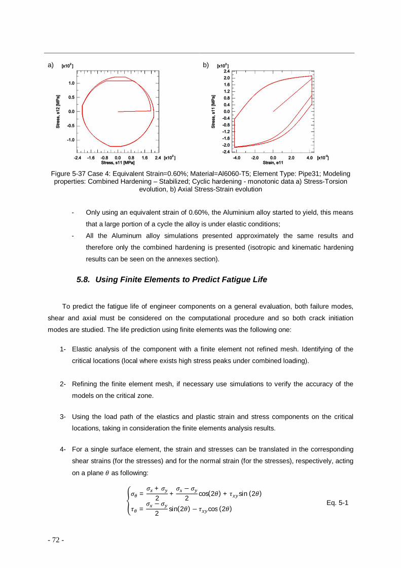
- 72 -
Figure 5-37 Case 4: Equivalent Strain=0.60%; Material=Al6060-T5; Element Type: Pipe31; Modeling properties: Combined Hardening – Stabilized; Cyclic hardening - monotonic data a) Stress-Torsion
evolution, b) Axial Stress-Strain evolution
- Only using an equivalent strain of 0.60%, the Aluminium alloy started to yield, this means
that a large portion of a cycle the alloy is under elastic conditions;
- All the Aluminum alloy simulations presented approximately the same results and
therefore only the combined hardening is presented (isotropic and kinematic hardening
results can be seen on the annexes section).
5.8. Using Finite Elements to Predict Fatigue Life
To predict the fatigue life of engineer components on a general evaluation, both failure modes,
shear and axial must be considered on the computational procedure and so both crack initiation
modes are studied. The life prediction using finite elements was the following one:
1- Elastic analysis of the component with a finite element not refined mesh. Identifying of the
critical locations (local where exists high stress peaks under combined loading).
2- Refining the finite element mesh, if necessary use simulations to verify the accuracy of the
models on the critical zone.
3- Using the load path of the elastics and plastic strain and stress components on the critical
locations, taking in consideration the finite elements analysis results.
4- For a single surface element, the strain and stresses can be translated in the corresponding
shear strains (for the stresses) and for the normal strain (for the stresses), respectively, acting
on a plane 휃 as following:
a)
b)
휎 =휎 + 휎
2 +휎 − 휎
2 cos(2휃) + 휏 sin (2휃)
휏 =휎 − 휎
2 sin(2휃) − 휏 cos (2휃) Eq. 5-1

- 73 -
5- Normal strain amplitude, ∆휀, distortion amplitude, ∆훾, and normal stress 휎 for each plane 휃
calculation through a load cycle.
6- Searching the 휃 plane where the maximum damage parameter occurs.
Using as an example the Fatemi Socie critical plane model:
7- Using the previous value it is possible to determine the fatigue life 푁 :
And finally iterating the eq. 5-4 it is find the number of cycles
Using the equation 5-1 for the Findley factor:
And for the Fatemi Socie factor comes that:
The table 5-2 shows the values for each material, result of the equation 5-5 and 5-6:
Table 5-2 Values of the material constants in the formulations of the Findley, and Fatemi-Socie
models
휀 =휀 + 휀
2 +휀 − 휀
2 cos(2휃) + 훾 sin (2휃)훾2 =
휀 − 휀2 sin(2휃)−
훾2 cos (2휃)
Eq. 5-2
푑 = 푚푎푥∆훾2 1 + 푘
휎 ,
휎 Eq. 5-3
푑 =휏퐺 2푁 + 훾 2푁 Eq. 5-4
휎 ,
휏 ,=
2
1 + 푘√1 + 푘
Eq. 5-5
푘 =
휏퐺 2푁 + 훾 2푁
1.3휎퐸 2푁 + 1.5휀 2푁
− 1퐾 0.002
휎 2푁 Eq. 5-6
Al 6060 T5 AISI 303
KF 0.19 0.2
KF-S 0.2 0.2
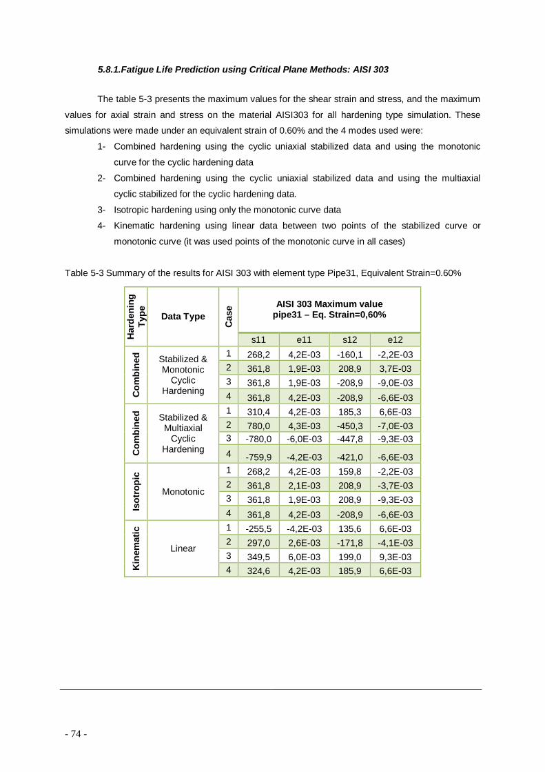
- 74 -
5.8.1. Fatigue Life Prediction using Critical Plane Methods: AISI 303
The table 5-3 presents the maximum values for the shear strain and stress, and the maximum
values for axial strain and stress on the material AISI303 for all hardening type simulation. These
simulations were made under an equivalent strain of 0.60% and the 4 modes used were:
1- Combined hardening using the cyclic uniaxial stabilized data and using the monotonic
curve for the cyclic hardening data
2- Combined hardening using the cyclic uniaxial stabilized data and using the multiaxial
cyclic stabilized for the cyclic hardening data.
3- Isotropic hardening using only the monotonic curve data
4- Kinematic hardening using linear data between two points of the stabilized curve or
monotonic curve (it was used points of the monotonic curve in all cases)
Table 5-3 Summary of the results for AISI 303 with element type Pipe31, Equivalent Strain=0.60%
Har
deni
ng
Type
Data Type
Cas
e AISI 303 Maximum value pipe31 – Eq. Strain=0,60%
s11 e11 s12 e12
Com
bine
d Stabilized & Monotonic
Cyclic Hardening
1 268,2 4,2E-03 -160,1 -2,2E-03 2 361,8 1,9E-03 208,9 3,7E-03 3 361,8 1,9E-03 -208,9 -9,0E-03 4 361,8 4,2E-03 -208,9 -6,6E-03
Com
bine
d Stabilized & Multiaxial
Cyclic Hardening
1 310,4 4,2E-03 185,3 6,6E-03 2 780,0 4,3E-03 -450,3 -7,0E-03 3 -780,0 -6,0E-03 -447,8 -9,3E-03 4 -759,9 -4,2E-03 -421,0 -6,6E-03
Isot
ropi
c
Monotonic
1 268,2 4,2E-03 159,8 -2,2E-03 2 361,8 2,1E-03 208,9 -3,7E-03 3 361,8 1,9E-03 208,9 -9,3E-03 4 361,8 4,2E-03 -208,9 -6,6E-03
Kin
emat
ic
Linear
1 -255,5 -4,2E-03 135,6 6,6E-03 2 297,0 2,6E-03 -171,8 -4,1E-03 3 349,5 6,0E-03 199,0 9,3E-03 4 324,6 4,2E-03 185,9 6,6E-03
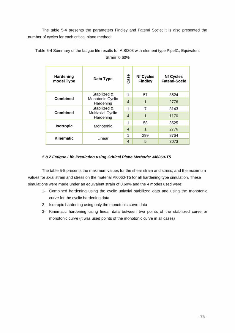
- 75 -
The table 5-4 presents the parameters Findley and Fatemi Socie; it is also presented the
number of cycles for each critical plane method:
Table 5-4 Summary of the fatigue life results for AISI303 with element type Pipe31, Equivalent
Strain=0.60%
5.8.2. Fatigue Life Prediction using Critical Plane Methods: Al6060-T5
The table 5-5 presents the maximum values for the shear strain and stress, and the maximum
values for axial strain and stress on the material Al6060-T5 for all hardening type simulation. These
simulations were made under an equivalent strain of 0.60% and the 4 modes used were:
1- Combined hardening using the cyclic uniaxial stabilized data and using the monotonic
curve for the cyclic hardening data
2- Isotropic hardening using only the monotonic curve data
3- Kinematic hardening using linear data between two points of the stabilized curve or
monotonic curve (it was used points of the monotonic curve in all cases)
Hardening model Type Data Type
Cas
e Nf Cycles Findley
Nf Cycles Fatemi-Socie
Combined Stabilized &
Monotonic Cyclic Hardening
1 57 3524
4 1 2776
Combined Stabilized &
Multiaxial Cyclic Hardening
1 7 3143
4 1 1170
Isotropic Monotonic 1 58 3525 4 1 2776
Kinematic Linear 1 299 3764 4 5 3073

- 76 -
Table 5-5 Summary of the results for Al6060-T5 with element type Pipe31, Equivalent Strain=0.60%
The table 5-6 presents the parameters Findley and Fatemi Socie; it is also presented the
number of cycles for each critical plane method:
Table 5-6 Summary of fatigue life results for Al6060-T5 with element type Pipe31, Equivalent
Strain=0.60%
Critical plane analysis
- Both materials presents approximately the same k value for both used critical plane
methods;
- The number of cycles using the Findley model is clearly lower than using the Fatemi
Socie. This large difference can be explained by the fact that the Findley model is more
accurate for high cycle fatigue.
Har
deni
ng
Type
Data Type
Cas
e
Al6060-T5 Maximum value Pipe31 – Eq. Strain=0,60%
s11 e11 s12 e12 C
ombi
ned Stabilized &
Monotonic Cyclic
Hardening
1 -159,2 -4,2E-03 -85,4 -6,6E-03 2 214,2 3,4E-03 -124,2 -5,4E-03 3 -218 -6,0E-03 -125,2 -9,4E-03 4 214 4,2E-03 -122,4 -6,6E-03
Isot
ropi
c
Monotonic
1 -147,4 -4,2E-03 -122,4 -6,6E-03 2 -200,5 -6,0E-03 115,8 9,4E-03 3 200,5 6,0E-03 115,7 9,4E-03 4 200,2 4,2E-03 -122,4 -6,6E-03
Kin
emat
ic
Linear
1 -145,7 4,2E-03 -79,7 -6,6E-03 2 198,4 6,0E-03 112,3 9,4E-03 3 198,5 6,0E-03 -114,2 -9,4E-03 4 194,4 4,2E-03 111,7 6,6E-03
Hardening model Type
Data Type
Cas
e Nf Cycles Findley
Nf Cycles Fatemi-Socie
Combined Stabilized &
Monotonic Cyclic Hardening
1 469 780
4 9 656
Isotropic Monotonic 1 612 798 4 12 674
Kinematic Linear 1 1179 811 4 27 694
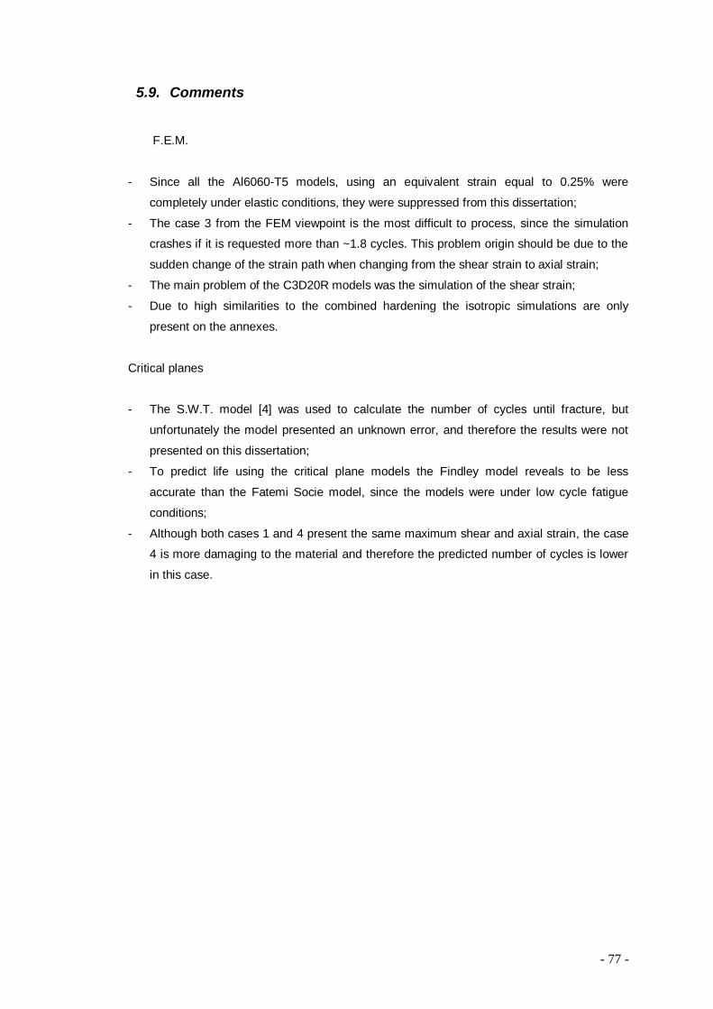
- 77 -
5.9. Comments
F.E.M.
- Since all the Al6060-T5 models, using an equivalent strain equal to 0.25% were
completely under elastic conditions, they were suppressed from this dissertation;
- The case 3 from the FEM viewpoint is the most difficult to process, since the simulation
crashes if it is requested more than ~1.8 cycles. This problem origin should be due to the
sudden change of the strain path when changing from the shear strain to axial strain;
- The main problem of the C3D20R models was the simulation of the shear strain;
- Due to high similarities to the combined hardening the isotropic simulations are only
present on the annexes.
Critical planes
- The S.W.T. model [4] was used to calculate the number of cycles until fracture, but
unfortunately the model presented an unknown error, and therefore the results were not
presented on this dissertation;
- To predict life using the critical plane models the Findley model reveals to be less
accurate than the Fatemi Socie model, since the models were under low cycle fatigue
conditions;
- Although both cases 1 and 4 present the same maximum shear and axial strain, the case
4 is more damaging to the material and therefore the predicted number of cycles is lower
in this case.

- 78 -

- 79 -
6. Conclusions
This chapter closes the dissertation, showing the most relevant conclusions of the work and also
some thoughts about the subjects studied.
Experimental:
- According to the experimental results of the uniaxial test (monotonic) and the cyclic
stabilized, the Aluminum alloy presents a steady behavior between the monotonic curve
and the cyclic hardening curve, the stainless steel between the same curves presented
only a hardening behavior;
- The experimental tests proved that the proportional tests under biaxial fatigue cause less
hardening than the biaxial nonproportional tests;
- The effects of the non proportionality was quantified using the additional hardening
coefficient 훼, for the AISI303 the final result was 0.9 [3] for the Aluminum alloy the result
was approximately 0.4;
- Since the additional hardening effect counts the effects of the rotation of the principal axis
during an out-phased solicitation this coefficient, should be taken in account in the life
prediction models to multiaxial fatigue.
F.E.M. conclusions:
- The pipe31 model proved to be a more accurate model than the C3D20R, the main
reason is the fact that with the C3D20R model it was not possible to produce a path shape
sufficiently approximated to the desire path in most of the cases;
- If using uniaxial data (monotonic curve) on the cyclic hardening data (on material
properties), the results of the FEM are not similar to the experimental results of the
nonproportional tests;
- If using cyclic multiaxial hardening data (linear trend line of the case 2-4 results) on the
CYCLIC HARDENING the FEM results are very similar to the experimental results, this
way it’s possible to diminish the effects previously mentioned;
- The finite element analysis proved that the local stress-strain cyclic responses are
different to different loading path. The graphics through different time have an important
part when studying the evolution and redistribution of the cyclic stress-strain fields;
- It was expected to analyze if the hardening for the Aluminum alloy was nearly the same
between under proportional and nonproportional loads, unfortunately only the case 4 for
an equivalent strain of ≈0.70% presented clearly plasticity;
- The critical plane method Fatemi Socie is more accurate to low cycle fatigue;
- To the both materials the case 4 is more damaging than the case 1.

- 80 -
- 81 -
References
[1] Borrego, L. P. A., L. M.; Costa, J. M.; Ferreira, J.M. (2004). "Analysis of Low Cycle Fatigue in
Al-Mg-Si Aluminium Alloys." Engineering failure Analysis 11: 715-725.
[2] Zhang, L., Wang, G., Cheng, J. e Jiang, L. Y. (2003). "Investigation of the Low-Cycle Fatigue
under Multiaxial NonProportional Loading." Materials Science and Engineering a - Structural
Materials Properties Microstructure and Processing 355(1-2): 18-23.
[3] Reis, L. F. G. d. (2004). "Comportamento Mecânico de Aços em Fadiga Multiaxial a Amplitude
de Carga Constante e Sincrona." Tese de Doutoramento em Engenharia Mecânica. Instituto
Superior Técnico. 2004
[4] Socie, D. F. and Marquis, G. B. “Multiaxial Fatigue”, Society of Automotive Engineers,
Warrendale, (2000) PA 15096-0001.
[5] Nishino, S., Hamada, N., Sakane, M., Ohnami, M., Matsumura, N. and Tokizane, M. (1986)
(1986). "Microstructural Study of Cyclic Strain Hardening Behaviour in Biaxial Stress State at
Elevated Temperature." Fatigue & Fracture of Engineering Materials & Structures 9: 65-77.
[6] Chung, K. L., M-G; Kim, D.; Wenner, M.L.; Barlat, F. (2005). "Spring-back evaluation of
automative sheets based on isotropic-kinematic hardenign laws and non-quadratic anisotropic
yield functions, Part I: theory and formulation." International Journal of Plasticity: 861-882
[7] Liu, Y. (2006). "A unified multiaxial fatigue damage model for isotropic and anisotropic
materials." International Journal of Fatigue 29: 347-359.
[8] Shang, D.-G. (2000). "A simple approach to the description of multiaxial cyclic stress-strain
relationship." International Journal of Fatigue 22: 251-256.
[9] Itoh, T. S., M.; Hata, T; Hamada, N. (2006). "A Design Procedure for Assessing Low Cycle
Fatigue Life under Proportional and Non-Proportional Loading." International Journal of
Fatigue 28: 459-466.
[10] Borodii, M. V. S., S.M. (2007). "Additional cyclic strain hardening and its relation to material,
structure, mechanical characteristics, and lifetime." 1184-1191.
[11] ABAQUS (1996a). "ABAQUS Theory Manual Version 5.7." HIBBITT, KARLSSON
&SORENSEN, INC
[12] Socie, D. F. (2001). "Multiaxial Fatigue - Theory."
[13] Doong, S. H., Socie, D. e Robertson, I. (1990). "Dislocation Substructures and
Nonproportional Hardening." Journal of Engineering Materials and Technology 112(4): 456-
464.
[14] Krempl, E. e Lu, H. (1989). "The Path and Amplitude Dependence of Cyclic Hardening of Type
304 Stainless Steel at Room Temperature." Biaxial and Multiaxial Fatigue, EGF 3: 89-106.
[15] Brown, M. W. e Miller, K. J. (1979). "Initiation and Growth of Cracks in Biaxial Fatigue."Fatigue
of Engineering Materials and Structures 1: 231-246.
[16] Matweb materials database properties. Consulted: April 2007, at: http://www.matweb.com
[17] ASTM E2207 (2003). "Standard Practice for Strain-Controlled Axial-Torsional FatigueTesting
with Thin-Walled Tubular Specimens - E 2207 - 02." ASTM Standards 03.01: 1-8.

- 82 -
[18] Standard Test Method for Vickers Hardness of Metallic Materials - ASTM E 92 – 82 (03)
[19] ASTM E606 (2003). "Standard Practice for Strain-Controlled Fatigue Testing - E 606 – 92
(Reapproved 1998)." ASTM Standards 03.01: 1-15.
[20] ABAQUS 6.7 Documentation, online
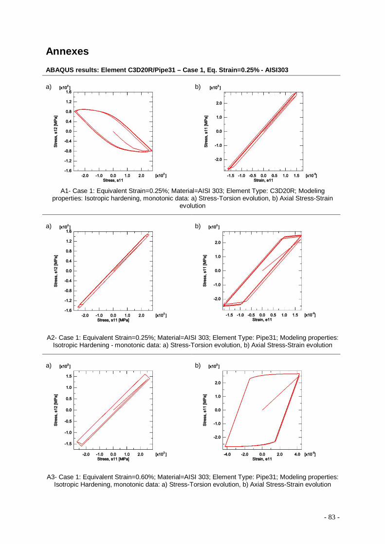
- 83 -
Annexes ABAQUS results: Element C3D20R/Pipe31 – Case 1, Eq. Strain=0.25% - AISI303
A1- Case 1: Equivalent Strain=0.25%; Material=AISI 303; Element Type: C3D20R; Modeling
properties: Isotropic hardening, monotonic data: a) Stress-Torsion evolution, b) Axial Stress-Strain evolution
A2- Case 1: Equivalent Strain=0.25%; Material=AISI 303; Element Type: Pipe31; Modeling properties:
Isotropic Hardening - monotonic data: a) Stress-Torsion evolution, b) Axial Stress-Strain evolution
A3- Case 1: Equivalent Strain=0.60%; Material=AISI 303; Element Type: Pipe31; Modeling properties:
Isotropic Hardening, monotonic data: a) Stress-Torsion evolution, b) Axial Stress-Strain evolution
a)
b)
a)
b)
a)
b)

- 84 -
ABAQUS results: Element C3D20R/Pipe31 – Case 2, Eq. Strain=0.25% - AISI303
A4- Case 2: Equivalent Strain=0.25%; Material- AISI 303; Element Type: C3D20R; Modeling
properties: Isotropic hardening, monotonic data: a) Stress-Torsion evolution, b) Axial Stress-Strain evolution
A5- Case 2: Equivalent Strain=0.25%; Material=AISI 303; Element Type: Pipe31; Modeling properties:
Isotropic Hardening - monotonic data: a) Stress-Torsion evolution, b) Axial Stress-Strain evolution
A6- Case 2: Equivalent Strain=0.60%; Material=AISI 303; Element Type: Pipe31; Modeling properties:
Isotropic Hardening, monotonic data: a) Stress-Torsion evolution, b) Axial Stress-Strain evolution
a)
b)
a)
b)
a)
b)

- 85 -
ABAQUS results: Element C3D20R/Pipe31 – Case 3, Eq. Strain=0.25% - AISI303
A7- Case 3: Equivalent Strain=0.25%; Material- AISI 303; Element Type: C3D20R; Modeling properties: Isotropic hardening, monotonic data: a) Stress-Torsion evolution, b) Axial Stress-Strain
evolution a)
b)
A8- Case 3: Equivalent Strain=0.25%; Material=AISI 303; Element Type: Pipe31; Modeling properties:
Isotropic Hardening - Stabilized Cyclic hardening - monotonic data: a) Stress-Torsion evolution, b) Axial Stress-Strain evolution
a)
b)
A9- Case 3: Equivalent Strain=0.60%; Material=AISI 303; Element Type: Pipe31; Modeling properties:
Isotropic Hardening, monotonic data: a) Stress-Torsion evolution, b) Axial Stress-Strain evolution
a)
b)

- 86 -
ABAQUS results: Element C3D20R/Pipe31 – Case 4, Eq. Strain=0.25% - AISI303 a)
b)
A10- Case 4: Equivalent Strain=0.25%; Material=AISI 303; Element Type: C3D20R; Modeling properties: Isotropic hardening, monotonic data: a) Stress-Torsion evolution, b) Axial Stress-Strain
evolution
A11- Case 4: Equivalent Strain=0.25%; Material=AISI 303; Element Type: Pipe31; Modeling
properties: Isotropic Hardening - monotonic data: a) Stress-Torsion evolution, b) Axial Stress-Strain evolution
A12- Case 4: Equivalent Strain=0.60%; Material=AISI 303; Element Type: Pipe31; Modeling properties: Isotropic Hardening, monotonic data: a) Stress-Torsion evolution, b) Axial Stress-Strain
evolution
a)
b)
a)
b)

- 87 -
ABAQUS results: Element Pipe31 – Case 1,2,3,4 Eq. Strain=0.60% - Al6060-T5 a)
b)
A13- Case 1: Equivalent Strain=0.60%; Material=Al6060-T5; Element Type: Pipe31; Modeling properties: Isotropic Hardening; monotonic data: a) Stress-Torsion evolution, b) Axial Stress-Strain
evolution
A14- Case 1: Equivalent Strain=0.60%; Material=Al6060-T5; Element Type: Pipe31; Modeling properties: Kinematic Hardening; Linear data: a) Stress-Torsion evolution, b) Axial Stress-Strain
evolution
A15- Case 2: Equivalent Strain=0.60%; Material=Al6060-T5; Element Type: Pipe31; Modeling properties: Kinematic Hardening; Linear data: a) Stress-Torsion evolution, b) Axial Stress-Strain
evolution
a)
b)
a)
b)
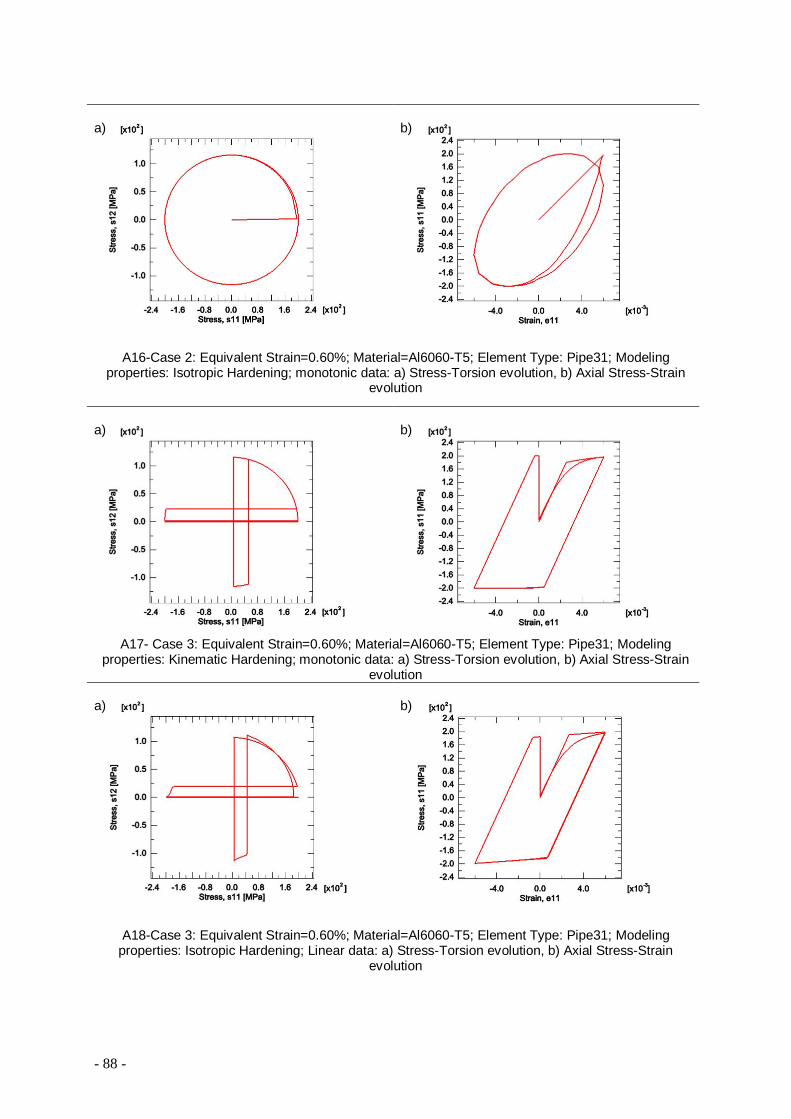
- 88 -
A16-Case 2: Equivalent Strain=0.60%; Material=Al6060-T5; Element Type: Pipe31; Modeling
properties: Isotropic Hardening; monotonic data: a) Stress-Torsion evolution, b) Axial Stress-Strain evolution
A17- Case 3: Equivalent Strain=0.60%; Material=Al6060-T5; Element Type: Pipe31; Modeling properties: Kinematic Hardening; monotonic data: a) Stress-Torsion evolution, b) Axial Stress-Strain
evolution a)
b)
A18-Case 3: Equivalent Strain=0.60%; Material=Al6060-T5; Element Type: Pipe31; Modeling
properties: Isotropic Hardening; Linear data: a) Stress-Torsion evolution, b) Axial Stress-Strain evolution
a)
b)
a)
b)
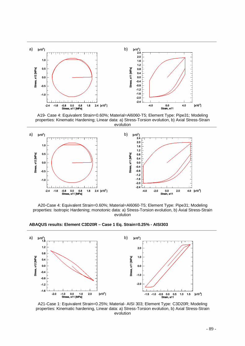
- 89 -
A19- Case 4: Equivalent Strain=0.60%; Material=Al6060-T5; Element Type: Pipe31; Modeling properties: Kinematic Hardening; Linear data: a) Stress-Torsion evolution, b) Axial Stress-Strain
evolution a)
b)
A20-Case 4: Equivalent Strain=0.60%; Material=Al6060-T5; Element Type: Pipe31; Modeling
properties: Isotropic Hardening; monotonic data: a) Stress-Torsion evolution, b) Axial Stress-Strain evolution
ABAQUS results: Element C3D20R – Case 1 Eq. Strain=0.25% - AISI303
A21-Case 1: Equivalent Strain=0.25%; Material- AISI 303; Element Type: C3D20R; Modeling
properties: Kinematic hardening, Linear data: a) Stress-Torsion evolution, b) Axial Stress-Strain evolution
a)
b)
a)
b)
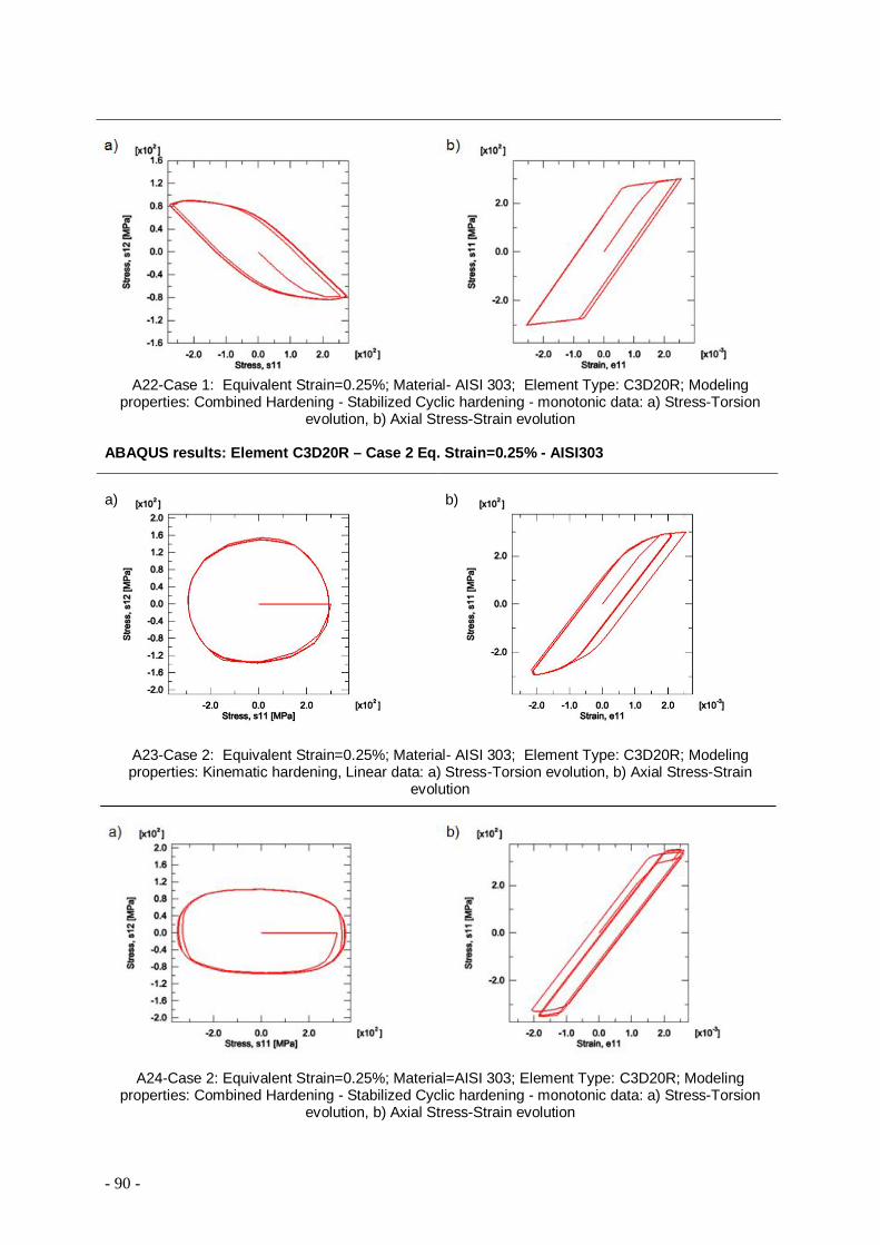
- 90 -
A22-Case 1: Equivalent Strain=0.25%; Material- AISI 303; Element Type: C3D20R; Modeling properties: Combined Hardening - Stabilized Cyclic hardening - monotonic data: a) Stress-Torsion
evolution, b) Axial Stress-Strain evolution
ABAQUS results: Element C3D20R – Case 2 Eq. Strain=0.25% - AISI303
A23-Case 2: Equivalent Strain=0.25%; Material- AISI 303; Element Type: C3D20R; Modeling properties: Kinematic hardening, Linear data: a) Stress-Torsion evolution, b) Axial Stress-Strain
evolution
A24-Case 2: Equivalent Strain=0.25%; Material=AISI 303; Element Type: C3D20R; Modeling properties: Combined Hardening - Stabilized Cyclic hardening - monotonic data: a) Stress-Torsion
evolution, b) Axial Stress-Strain evolution
a)
b)
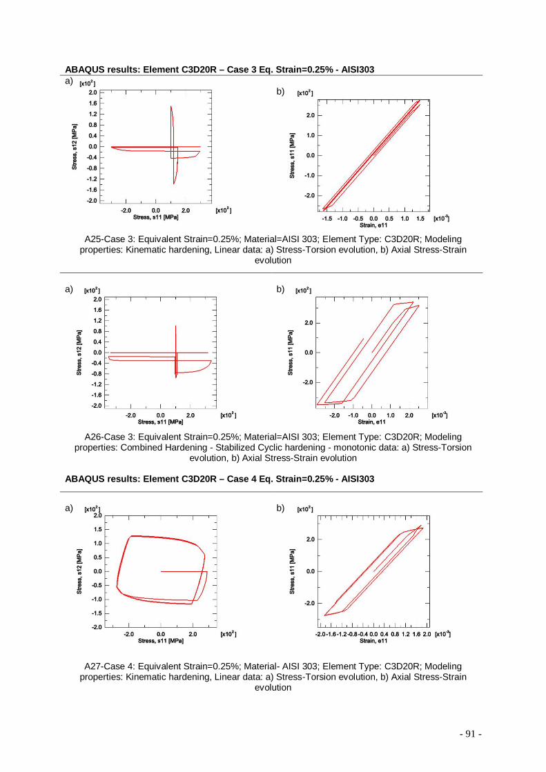
- 91 -
ABAQUS results: Element C3D20R – Case 3 Eq. Strain=0.25% - AISI303 a)
b)
A25-Case 3: Equivalent Strain=0.25%; Material=AISI 303; Element Type: C3D20R; Modeling properties: Kinematic hardening, Linear data: a) Stress-Torsion evolution, b) Axial Stress-Strain
evolution
A26-Case 3: Equivalent Strain=0.25%; Material=AISI 303; Element Type: C3D20R; Modeling
properties: Combined Hardening - Stabilized Cyclic hardening - monotonic data: a) Stress-Torsion evolution, b) Axial Stress-Strain evolution
ABAQUS results: Element C3D20R – Case 4 Eq. Strain=0.25% - AISI303
A27-Case 4: Equivalent Strain=0.25%; Material- AISI 303; Element Type: C3D20R; Modeling
properties: Kinematic hardening, Linear data: a) Stress-Torsion evolution, b) Axial Stress-Strain evolution
a)
b)
a)
b)

- 92 -
A28-Case 4: Equivalent Strain=0.25%; Material- AISI 303; Element Type: C3D20R; Modeling
properties: Combined Hardening - Stabilized Cyclic hardening - monotonic data: a) Stress-Torsion evolution, b) Axial Stress-Strain evolution
a)
b)

- 93 -
Fatigue life results: Element C3D20R – Eq. Strain=0.25% - AISI303
B1 - Summary of the stress and strain results for AISI 303 with element type C3D20R, Equivalent
Strain=0.25%
B2- Summary of the fatigue life results for AISI 303 with element type C3D20R, Equivalent
Strain=0.25%
Har
deni
ng
Type
Data Type
Cas
e AISI 303 Maximum value C3D20R – Eq. Strain=0,25%
s11 e11 s12 e12
Com
bine
d Stabilized &
Monotonic Cyclic
Hardening
1 -275,6 -1,6E-03 89,8 1,4E-03 2 -350,5 -1,8E-03 102,8 1,5E-03 3 -349,4 -2,9E-03 103,2 1,5E-03 4 329,5 1,9E-03 96,4 1,2E-03
Isot
ropi
c
Monotonic
1 276,7 1,5E-03 90,3 1,2E-03 2 -350,5 -1,8E-03 102,8 1,5E-03 3 -349,4 -2,9E-03 103,2 1,5E-03 4 329,5 1,9E-03 97,5 1,1E-03
Kin
emat
ic
Linear
1 240,9 1,6E-03 99,9 1,8E-03 2 300,8 2,6E-03 154,8 1,6E-03 3 -300,8 -2,6E-03 151,3 2,2E-03 4 289,8 1,8E-03 128,1 1,5E-03
Hardening model Type Data Type
Cas
e Nf Cycles Findley
Nf Cycles Fatemi-Socie
Combined Stabilized &
Monotonic Cyclic Hardening
1 1318 404410
4 126 163200
Isotropic Monotonic 1 1234 665601 4 121 149287
Kinematic Linear 1 3081 431656 4 144 218963
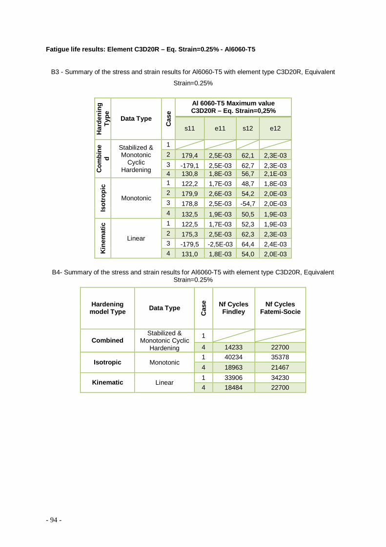
- 94 -
Fatigue life results: Element C3D20R – Eq. Strain=0.25% - Al6060-T5
B3 - Summary of the stress and strain results for Al6060-T5 with element type C3D20R, Equivalent
Strain=0.25%
B4- Summary of the stress and strain results for Al6060-T5 with element type C3D20R, Equivalent Strain=0.25%
Har
deni
ng
Type
Data Type
Cas
e
Al 6060-T5 Maximum value C3D20R – Eq. Strain=0,25%
s11 e11 s12 e12
Com
bine
d
Stabilized & Monotonic
Cyclic Hardening
1 2 179,4 2,5E-03 62,1 2,3E-03 3 -179,1 2,5E-03 62,7 2,3E-03 4 130,8 1,8E-03 56,7 2,1E-03
Isot
ropi
c
Monotonic
1 122,2 1,7E-03 48,7 1,8E-03 2 179,9 2,6E-03 54,2 2,0E-03 3 178,8 2,5E-03 -54,7 2,0E-03 4 132,5 1,9E-03 50,5 1,9E-03
Kin
emat
ic
Linear
1 122,5 1,7E-03 52,3 1,9E-03 2 175,3 2,5E-03 62,3 2,3E-03 3 -179,5 -2,5E-03 64,4 2,4E-03 4 131,0 1,8E-03 54,0 2,0E-03
Hardening model Type Data Type
Cas
e Nf Cycles Findley
Nf Cycles Fatemi-Socie
Combined Stabilized &
Monotonic Cyclic Hardening
1
4 14233 22700
Isotropic Monotonic 1 40234 35378 4 18963 21467
Kinematic Linear 1 33906 34230 4 18484 22700
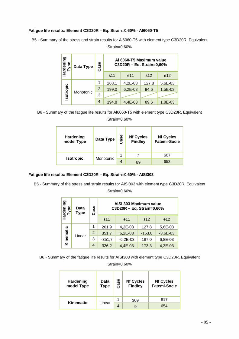
- 95 -
Fatigue life results: Element C3D20R – Eq. Strain=0.60% - Al6060-T5
B5 - Summary of the stress and strain results for Al6060-T5 with element type C3D20R, Equivalent
Strain=0.60%
B6 - Summary of the fatigue life results for Al6060-T5 with element type C3D20R, Equivalent
Strain=0.60%
Fatigue life results: Element C3D20R – Eq. Strain=0.60% - AISI303
B5 - Summary of the stress and strain results for AISI303 with element type C3D20R, Equivalent
Strain=0.60%
B6 - Summary of the fatigue life results for AISI303 with element type C3D20R, Equivalent
Strain=0.60%
Har
deni
ng
Type
Data Type
Cas
e Al 6060-T5 Maximum value C3D20R – Eq. Strain=0,60%
s11 e11 s12 e12
Isot
ropi
c
Monotonic
1 268,1 4,2E-03 127,8 5,6E-03 2 199,0 6,2E-03 94,6 1,5E-03 3 4 194,8 4,4E-03 89,6 1,8E-03
Hardening model Type Data Type
Cas
e Nf Cycles Findley
Nf Cycles Fatemi-Socie
Isotropic Monotonic 1 2 607 4 89 653
Har
deni
ng
Type
Data Type C
ase AISI 303 Maximum value
C3D20R – Eq. Strain=0,60%
s11 e11 s12 e12
Kin
emat
ic
Linear
1 261,9 4,2E-03 127,8 5,6E-03 2 351,7 6,2E-03 -163,0 -3,6E-03 3 -351,7 -6,2E-03 187,0 6,8E-03 4 326,2 4,4E-03 173,3 4,3E-03
Hardening model Type
Data Type C
ase Nf Cycles
Findley Nf Cycles
Fatemi-Socie
Kinematic Linear 1 309 817 4 9 654

- 96 -
Fatigue life results: Element Pipe31 – Eq. Strain=0.25% - AISI303
B5 - Summary of the stress and strain results for AISI303 with element type Pipe31, Equivalent
Strain=0.25% B6 - Summary of the fatigue life results for AISI303 with element type Pipe31, Equivalent Strain=0.25%
Har
deni
ng
Type
Data Type
Cas
e AISI 303 Maximum value pipe31 – Eq. Strain=0,25%
s11 e11 s12 e12
Com
bine
d Stabilized & Monotonic
Cyclic Hardening
1 254,2 1,8E-03 151 1,6E-03 2 361,8 2,0E-03 208,9 3,2E-03 3 -353,6 -2,5E-03 -206,5 -3,9E-03 4 317 1,8E-03 -181,1 -2,8E-03
Com
bine
d Stabilized & Multiaxial
Cyclic Hardening
1 292,8 1,8E-03 173,4 2,8E-03 2 530 2,5E-03 -294,8 -3,8E-03 3 448,7 2,5E-03 -266,8 -3,9E-03 4 347,2 1,8E-03 -207,1 -2,8E-03
Isot
ropi
c
Monotonic
1 254,2 1,8E-03 151 1,6E-03 2 -361,8 -2,0E-03 -208,9 -3,1E-03 3 -353,7 -2,5E-03 -206,5 -3,9E-03 4 317 1,8E-03 -181,2 -2,8E-03
Kin
emat
ic
Linear
1 -215,6 -1,8E-03 121,6 2,7E-03 2 -290,1 -1,8E-03 170,7 3,4E-03 3 299,9 2,5E-03 -172,3 -3,9E-03 4 281,6 1,8E-03 -161,9 -2,8E-03
Hardening model Type Data Type
Cas
e Nf Cycles Findley
Nf Cycles Fatemi-Socie
Combined Stabilized &
Monotonic Cyclic Hardening
1 127 234830
4 8 101754
Combined Stabilized &
Multiaxial Cyclic Hardening
1 17 207225
4 1 86065
Isotropic Monotonic 1 127 234830 4 7 101754
Kinematic Linear 1 2059 275134 4 39 119779