measuring the strength of metalsmedia.public.gr/books-pdf/9781118413418-0831211.pdf · 2 measuring...

1

CHAPTER 1

MEASURING THE STRENGTHOF METALS

Fundamentals of Strength: Principles, Experiment, and Applications of an Internal State Variable Constitutive Formulation, First Edition. Paul S. Follansbee.© 2014 The Minerals, Metals & Materials Society. Published 2014 by John Wiley & Sons, Inc.

The strength of metals is a fascinating topic that carries engineering and

scientifi c implications. You cannot build a bridge, design a turbine blade, or

construct a transmission line tower without understanding the strength of the

materials of construction in balance with the requirements of the system.

1.1 HOW IS STRENGTH MEASURED?

Let us take a piece of metal and machine a test specimen of either the geometry

shown in Figure 1.1 or Figure 1.2 . Note that two geometries are shown. At the

center point of these specimens, one has a circular cross section, whereas the

other has a rectangular cross section. Either geometry can be used according

to the material stock available.

After machining, this sample is attached to the “grips” of a test machine.

An example of a testing machine is shown in Figure 1.3 . This is an “electrome-

chanical” machine in that the moving crosshead is attached to very large

screws (in the columns) that move the crosshead up or down with great force.

The test specimen is mounted between the two grips.

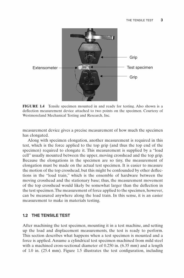
Figure 1.4 shows a test specimen mounted between two grips. It also

shows a “defl ection measurement device” attached to the specimen. As

force is applied to the top grip and the specimen elongates, the defl ection

COPYRIG

HTED M

ATERIAL

2 MEASURING THE STRENGTH OF METALS

FIGURE 1.1 Test specimen machined from a plate thick enough to give a circular

cross section. Courtesy of Westmoreland Mechanical Testing and Research, Inc.

(WMT&R, Inc.).

FIGURE 1.2 Test specimen machined from a plate that is too thin to give a large-

enough circular cross section. Courtesy of Westmoreland Mechanical Testing and

Research, Inc.

FIGURE 1.3 Mechanical test frame with top and bottom grips. Courtesy of West-

moreland Mechanical Testing and Research, Inc.

Moving

crosshead

Grip

Tensilespecimen with

extensometer

Data acquisitionsystem and test

machine controls

Grip

THE TENSILE TEST 3

measurement device gives a precise measurement of how much the specimen

has elongated.

Along with specimen elongation, another measurement is required in this

test, which is the force applied to the top grip (and thus the top end of the

specimen) required to elongate it. This measurement is supplied by a “load

cell” usually mounted between the upper, moving crosshead and the top grip.

Because the elongations in the specimen are so tiny, the measurement of

elongation must be made on the actual test specimen. It is easier to measure

the motion of the top crosshead, but this might be confounded by other defl ec-

tions in the “load train,” which is the ensemble of hardware between the

moving crosshead and the stationary base; thus, the measurement movement

of the top crosshead would likely be somewhat larger than the defl ection in

the test specimen. The measurement of force applied to the specimen, however,

can be measured anywhere along the load train. In this sense, it is an easier

measurement to make in materials testing.

1.2 THE TENSILE TEST

After machining the test specimen, mounting it in a test machine, and setting

up the load and displacement measurements, the test is ready to perform.

This section describes what happens when a test specimen is mounted and a

force is applied. Assume a cylindrical test specimen machined from mild steel

with a machined cross-sectional diameter of 0.250 in. (6.35 mm) and a length

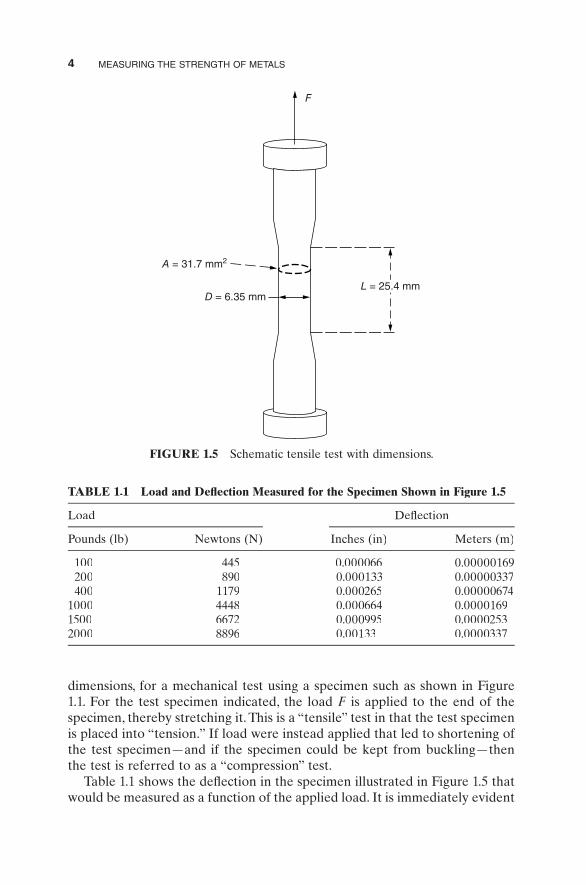
of 1.0 in. (25.4 mm). Figure 1.5 illustrates the test confi guration, including

FIGURE 1.4 Tensile specimen mounted in and ready for testing. Also shown is a

defl ection measurement device attached to two points on the specimen. Courtesy of

Westmoreland Mechanical Testing and Research, Inc.

Grip

Grip

Extensometer Test specimen


dimensions, for a mechanical test using a specimen such as shown in Figure

1.1 . For the test specimen indicated, the load F is applied to the end of the Fspecimen, thereby stretching it. This is a “tensile” test in that the test specimen

is placed into “tension.” If load were instead applied that led to shortening of

the test specimen—and if the specimen could be kept from buckling—then

the test is referred to as a “compression” test.

Table 1.1 shows the defl ection in the specimen illustrated in Figure 1.5 that

would be measured as a function of the applied load. It is immediately evident

FIGURE 1.5 Schematic tensile test with dimensions.

F

A = 31.7 mm2

D = 6.35 mmL = 25.4 mm

TABLE 1.1 Load and Defl ection Measured for the Specimen Shown in Figure 1.5

Load Defl ection

Pounds (lb) Newtons (N) Inches (in) Meters (m)

100 445 0.000066 0.00000169200 890 0.000133 0.00000337400 1179 0.000265 0.00000674

1000 4448 0.000664 0.00001691500 6672 0.000995 0.00002532000 8896 0.00133 0.0000337

THE TENSILE TEST 5

that even with what appears to be very large forces on this test specimen, the

defl ections are quite small. With 1 ton of force pulling on the specimen, the

specimen only elongates 1.33 mils (33.7 μm).

Figure 1.6 plots the load versus the defl ection—as if a defl ection measure-

ment were taken for every 100-lb increase in load. (Even though defl ection has

been defi ned as the dependent variable, which would normally be plotted on

the y -axes, Figure 1.6 plots defl ection on the x -axis; this will be made clear later.)

It is evident in Figure 1.6 that the force-versus-defl ection measurements plot

on a straight line. Recall from general physics that the behavior illustrated in

Figure 1.6 is analogous to the behavior of a spring, defi ned by the familiar

equation

F K XS= Δ , (1.1)

where F is the applied force and F ΔX is the extension of the spring. In fact, theXtest specimen does behave like a spring. However, this test specimen is indeed

a strong spring. Simple springs used in general physics laboratory experiments

typically have spring constants on the order of ∼ 10 N/m. As a comparison, the

test specimen is a spring with a spring constant of

KFX

S = =×

= ×−Δ

8896

3 37 102 64 10

5

8N

m

N

m.. .

Thus, as a spring, the test specimen has a spring constant ∼20 million times

larger than the springs used in a common physics laboratory. When materials

FIGURE 1.6 Force (as MN or 10 6 N) plotted versus defl ection (as μm or 10 −6 m) for

the specimen shown in Figure 1.5 .

10,000

6,000

8,000

4,000

Force (N)

0

2,000

0.0 10.0 20.0 30.0 40.0

Deflection (μm)


behave like this during a tensile test, they are said to be behaving as an “elastic”

solid.

Just as with any spring, if the force on our tensile specimen is reduced, the

elongation decreases until it reaches zero extension when the force goes to

zero.

1.3 STRESS IN A TEST SPECIMEN

Imagine that the test specimen had a diameter of 0.500 in. (12.7 mm) instead

of 0.250 in. (6.35 mm). One would expect that the spring constant of our test

specimen would get even larger, and the same force would cause less elonga-

tion. To eliminate the effect of specimen size, the force, F , is divided by theFFcross-sectional area, A, to yield a “stress,” σe, wheree

σe =FA

. (1.2)

Of course, stress in general is force divided by area. When deformation

increases as shown in Figure 1.6 —which implies the specimen geometry

changes—but stress is computed by dividing the force by the original area, then

the stress is referred to as the engineering stress , which is why a subscript “e” is

used in Equation (1.2) . Later (Section 1.10 ), the stress will be based on the

current area. If F has the unit of newton and F A has the unit of square meter, then

the stress σe has the unit newton per square meter, which is known as a pascal:

PaN

m=

2.

A pascal is a very small stress. Recall that the units of pressure are also

force per unit area. Standard atmospheric air pressure is ∼ 105 Pa. Thus, stresses

in test specimens are more commonly stated in terms of 10 6 Pa or MPa. The

engineering units for stress are pounds per square inch, or psi. Standard atmo-

spheric air pressure is 14.7 psi. Accordingly, when using engineering units,

stresses in test specimens are commonly stated in terms of 103 psi or ksi. The

conversion between MPa and ksi is

MPaksi

=0 145.

. (1.3)

1.4 STRAIN IN A TEST SPECIMEN

Suppose the test specimen was machined with a length of 2.0 in. (50.8 mm)

instead of 1.0 in. (25.4 mm). The same force would produce an extension in

THE ELASTIC STRESS VERSUS STRAIN CURVE 7

the 2.0-in.-long test specimen that is twice that in the 1.0-in.-long test specimen.

To eliminate the effect of specimen length, L , on the test result, the extension,

ΔL, is measured relative to the specimen ’ s length:

εe =ΔLL

. (1.4)

This relative extension is referred to as the “strain” εe . Note that since e ΔLand L have the same units, the ratio εe is dimensionless. As in the calculation

of stress, when strain is based on the initial specimen length, the value is

referred to as the engineering strain denoted by the subscript “e.”

1.5 THE ELASTIC STRESS VERSUS STRAIN CURVE

Since the cross-sectional area of the test specimen (with a diameter of 0.250 in.

or 6.35 mm) and the length of the test specimen (1.0 in. or 25.4 mm) are known,

the force versus extension curve can easily be converted to stress versus strain

for the tensile test shown earlier. The resulting stress versus strain curve is

shown in Figure 1.7 .

Note that there are no units shown for strain, which is a dimensionless

quantity, and that the units for stress are MPa (or 10 6 Pa or 10 6 N/m 2 ). Other

than this, the curve appears identical to that shown in Figure 1.6 . The differ-

ence is that if a specimen with a diameter of 0.500 in. instead of 0.250 in. or

a specimen with a length of 2.0 in. instead of 1.0 in. had been used, the result-

ing stress versus strain curves would have been identical; that is, converting

from force to stress and extension to strain has eliminated specimen geometry

effects.

FIGURE 1.7 Stress versus strain for the specimen shown in Figure 1.5 .

300

200

Stress(MPa)

100

00.0000 0.0005 0.0010 0.0015

Strain


1.6 THE ELASTIC MODULUS

Given the curve shown in Figure 1.7 is geometry invariant, the slope of this

line rather than the slope of the line in Figure 1.6 takes on special meaning.

This slope is defi ned as the “elastic modulus.” It is also referred to as Young ’ s

modulus, named after a nineteenth century British scientist. In fact, the equa-

tion for the line in Figure 1.7 is

σ εe e= E (1.5)

σ εe e= = =FA

E EL

LΔ

, (1.6)

where E is the elastic modulus. Because E εe in this equation is dimensionless, Ehas the unit of σe , which, as discussed earlier, is newton per square meter ore

pascal. From the plot in Figure 1.6 , E for this steel is 30.7 E × 10 6 psi (212 × 10 9 Pa).

It turns out that E is a fundamental physical property of metals and ceram-Eics. It is defi ned by interatomic forces and varies from material to material.

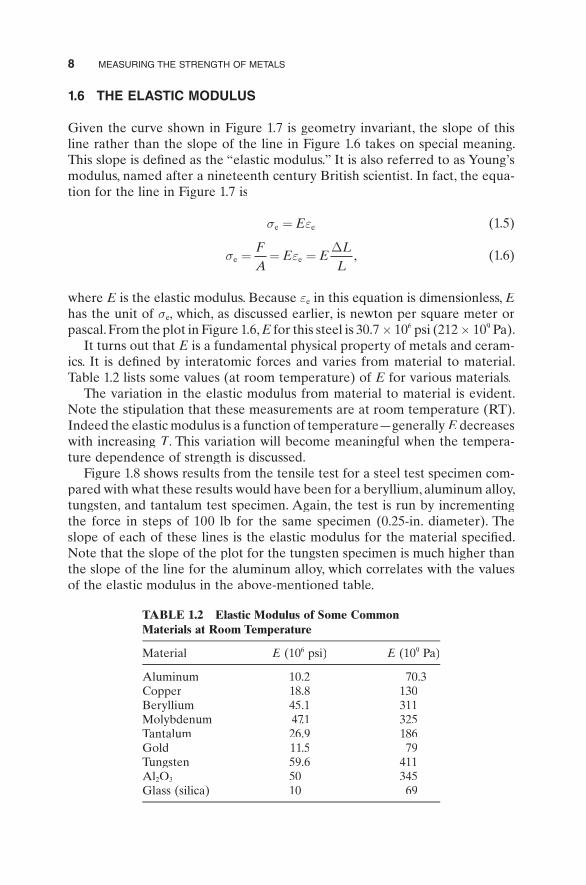
Table 1.2 lists some values (at room temperature) of E for various materials.E The variation in the elastic modulus from material to material is evident.

Note the stipulation that these measurements are at room temperature ( RT ).

Indeed the elastic modulus is a function of temperature—generally E decreases Ewith increasing T . This variation will become meaningful when the tempera-TTture dependence of strength is discussed.

Figure 1.8 shows results from the tensile test for a steel test specimen com-

pared with what these results would have been for a beryllium, aluminum alloy,

tungsten, and tantalum test specimen. Again, the test is run by incrementing

the force in steps of 100 lb for the same specimen (0.25-in. diameter). The

slope of each of these lines is the elastic modulus for the material specifi ed.

Note that the slope of the plot for the tungsten specimen is much higher than

the slope of the line for the aluminum alloy, which correlates with the values

of the elastic modulus in the above-mentioned table.

TABLE 1.2 Elastic Modulus of Some CommonMaterials at Room Temperature

Material E (10 E 6 psi) E (10E 9 Pa)

Aluminum 10.2 70.3Copper 18.8 130Beryllium 45.1 311Molybdenum 47.1 325Tantalum 26.9 186Gold 11.5 79Tungsten 59.6 411Al2 O3 50 345Glass (silica) 10 69

LATERAL STRAINS AND POISSON’S RATIO 9

1.7 LATERAL STRAINS AND P OISSON ’ S RATIO

For the tensile tests described earlier, a defl ection measuring device—also

known as an extensometer—was attached to measure axial defl ection, which rwas converted to strain. How about the strain in the radial direction (for the

case of a cylindrical test specimen)? If volume is conserved during the test,

then this can be estimated. Assume the initial and fi nal diameters of the test

specimen are D and Df and that the initial and fi nal lengths are f L and Lf.fAccordingly, when volume is conserved,

L D L D

LL

DD

L LL

LL

DD

π π

ε

4 42 2

2

2

=

=⎛⎝⎜⎜⎜

⎞⎠⎟⎟⎟

−= = =

⎛⎝⎜⎜⎜

⎞⎠⎟⎟⎟

f f

f

f

fe

f

Δ−−

= +( )

=+( )

−= =

+( )−

1

1

1

1

1

11

1 2

1 2

1 2

DDDD

D DD

f

e

f

e

feD

e

ε

ε

εε

,

Stress versus strain for fi ve metals with differing values of the elastic

modulus.

1000

800

Mild steel

Aluminum 6061

Tantalum

Tungsten

Stress(MPa)

400

600Beryllium

0

200

0 0.0005 0.001 0.0015 0.002 0.0025

Strain


where εeD is defi ned as the strain in the direction of the diameter of the test

specimen. The fi rst term in the equation can be estimated using a binomial

series approximation:

εε

ε εeD

e

e e=+( )

− ≅ −⎛⎝⎜⎜⎜

⎞⎠⎟⎟⎟− = −

1

11 1

21

21 2. (1.7)

When volume is conserved, the strain in the direction of the diameter—the

diametrical strain—is one-half the axial strain—and it is of opposite sign. The lratio of the diametrical strain to the axial strain is

εεeD

e

= −1

2. (1.8)

The negative of this ratio is called Poisson ’ s ratio , ν , named after the Frenchνmathematician Siméon Poisson:

νεε

= − eD

e

. (1.9)

This derivation, however, assumed that the volume remains constant

throughout the test. Materials that behave like this are referred to as “incom-

pressible.” However, most materials are not incompressible but have a very

small change in volume when elastically deformed. In fact, Table 1.3 summa-

rizes typical values of Poisson ’ s ratio for metals, ceramics, and polymers.

How much does the volume and density change? Taking the example tensile

test on a steel test specimen (which has a Poisson ’ s ratio of 0.33) shown in

Figure 1.7 , the volume would be

VV

D LD L

DD

LL

F F F F F

e

0

2

02

0 0

2

0

1

= =⎛⎝⎜⎜⎜

⎞⎠⎟⎟⎟

⎛⎝⎜⎜⎜

⎞⎠⎟⎟⎟

= −( )

ππ

νεmax

221+( )εemax ,

where V0VV and VFVV are the initial and fi nal volumes, respectively, and εemax is the

maximum strain. Taking εemax .= 0 0013 from Figure 1.7 ,

TABLE 1.3 Poisson ’ s Ratios for Metals, Ceramics, and Polymers Differ and Are in the Ranges Shown

Material Poisson ’ s Ratio ν

Metals ∼ 0.33Ceramics ∼ 0.25Polymers ∼ 0.40

DEFINING STRENGTH 11

VV

F

0

21 0 33 0 0013 1 0 0013 1 00044= − ×( ) +( ) =. . . . ,

which shows the volume increases (thus, the density decreases) by 0.044%.

Thus, the metal is compressible during elastic loading, but the change in

volume is very small.

1.8 DEFINING STRENGTH

One should wonder now whether a tensile specimen can be stretched elasti-

cally even further than shown in Figure 1.6 , Figure 1.7 , and Figure 1.8 . Intui-

tively, the answer of course is no; eventually, the test specimen will break.

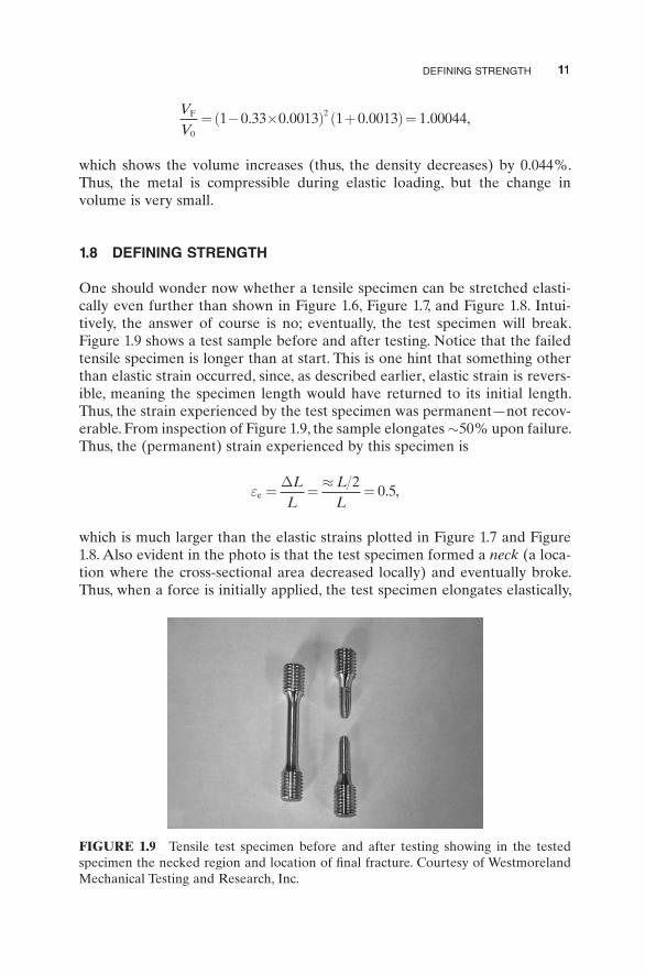
Figure 1.9 shows a test sample before and after testing. Notice that the failed

tensile specimen is longer than at start. This is one hint that something other

than elastic strain occurred, since, as described earlier, elastic strain is revers-

ible, meaning the specimen length would have returned to its initial length.

Thus, the strain experienced by the test specimen was permanent—not recov-

erable. From inspection of Figure 1.9 , the sample elongates ∼ 50% upon failure.

Thus, the (permanent) strain experienced by this specimen is

εe = =≈

=ΔLL

LL

20 5. ,

which is much larger than the elastic strains plotted in Figure 1.7 and Figure

1.8 . Also evident in the photo is that the test specimen formed a neck (a loca-

tion where the cross-sectional area decreased locally) and eventually broke.

Thus, when a force is initially applied, the test specimen elongates elastically,

FIGURE 1.9 Tensile test specimen before and after testing showing in the tested

specimen the necked region and location of fi nal fracture. Courtesy of Westmoreland

Mechanical Testing and Research, Inc.


but eventually, the specimen experiences permanent strain. The transition

between these two processes is one defi nition of strength.

There was actually a hint regarding this defi nition of strength in Figure 1.8 ,

when the lines were only plotted to a specifi c value of strain (or stress). The

aluminum line was plotted only to a strain of only ∼ 0.00065, whereas the

tungsten line was plotted all the way to a strain of ∼0.0025. The reason is that

this maximum strain is the point on each curve where this transition occurs.

1.9 STRESS–STRAIN CURVE

To better understand the full stress–strain curve, it is useful to view an actual

data set. First, since the example used is from a compression test rather than

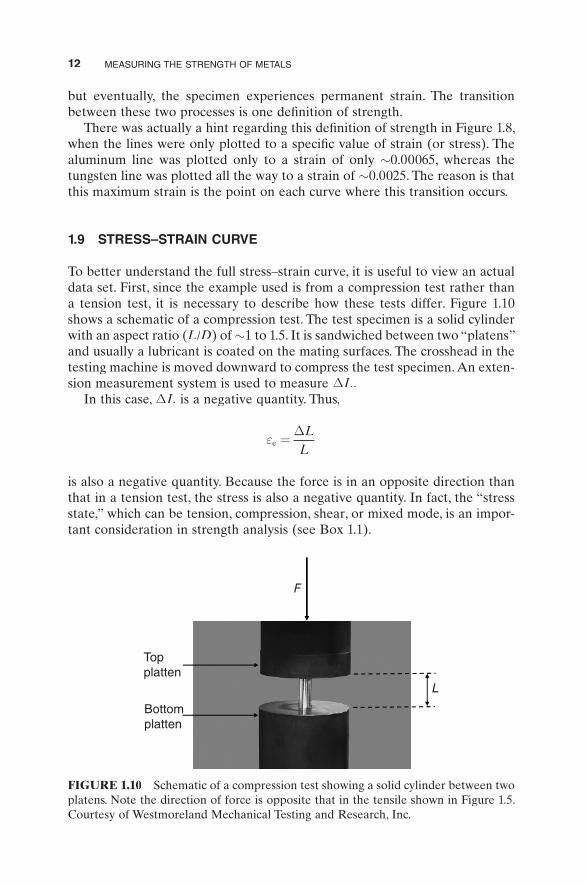
a tension test, it is necessary to describe how these tests differ. Figure 1.10

shows a schematic of a compression test. The test specimen is a solid cylinder

with an aspect ratio (L /D ) of ∼ 1 to 1.5. It is sandwiched between two “platens”

and usually a lubricant is coated on the mating surfaces. The crosshead in the

testing machine is moved downward to compress the test specimen. An exten-

sion measurement system is used to measure ΔL .

In this case, ΔL is a negative quantity. Thus,

εe =ΔLL

is also a negative quantity. Because the force is in an opposite direction than

that in a tension test, the stress is also a negative quantity. In fact, the “stress

state,” which can be tension, compression, shear, or mixed mode, is an impor-

tant consideration in strength analysis (see Box 1.1 ).

FIGURE 1.10 Schematic of a compression test showing a solid cylinder between two

platens. Note the direction of force is opposite that in the tensile shown in Figure 1.5 .

Courtesy of Westmoreland Mechanical Testing and Research, Inc.

F

Top

Lplatten

Bottom

platten

STRESS–STRAIN CURVE 13

Box 1.1 Stress State

As illustrated in the fi gure on the left, stress is a tensor quantity comprised

in a general x , y, z coordinate system of three normal stresses— σxσ , σyσ , and

σz—and three shear stresses— τxyτ , τyzτ , and τxzτ .

1

2

3σzσ

yσ

xσxyτ

xzτ

yzτ

σ

σ

The principal coordinate system (on the right) is one where the principal stresses σ1, σ2 , and σ3 are normal to the three planes and the shear stress

components on these planes are zero. Uniaxial tension and compression

tests represent the case where the stress axis is a principal stress axis and

σ2 and σ3 equal zero. Of course, in a tensile test, σ1 is a positive quantity,

whereas in a compression test, it is a negative quantity. There are a myriad

of stress states that are used in mechanical testing. The following fi gure

shows the case on the left of a plane stress test on a thin sheet, where σ3 = 0

and σ1 and σ2 can take on any (positive) values, and on the right, a torsion

test on a tube, where σ1 = −σ2 = τ and τ σ3 = 0.

σ

1

1 2

2

1

σ2

σ σ

σσ


The elastic loading behavior for our steel compression specimen is as shown

in Figure 1.11 . Per convention, the stress and strain start at zero, but as the

sample compresses, the stress and strain increase in a negative direction.

Figure 1.12 shows the measured stress–strain curve in a 1018 steel compres-

sion test specimen [1] . The solid line is the measurement of force and extension

converted to stress and strain as discussed earlier. The dashed line is the elastic

loading line plotted in Figure 1.11 . Because the full-scale value of strain in

Figure 1.12 is −0.10 whereas that in Figure 1.11 was −0.0015, the elastic line

in Figure 1.12 seems to have a much higher slope. It actually is the same line.

How about the “bumps and wiggles” on the measured curve? More than

likely in this case, these represent “noise,” for example, electronic noise, in the

FIGURE 1.11 Stress versus strain in the elastic regime for a compression test in 1018

steel.

0–0.0015 –0.0010 –0.0005 0.0000

Strain

–100

–200

Stress(MPa)

–300

FIGURE 1.12 Compression test in 1018 steel showing stress versus strain up to a

strain of −10%.

–0.1 –0.08 –0.04 –0.02 0

Strain

–200

0–0.06

Elastic behavior

–400

Stress(MPa)

–600

1018 steel

–800

STRESS–STRAIN CURVE 15

measurement system, although there are examples where features such as

these may actually refl ect a metallurgical process.

The key point in Figure 1.12 is that the measured behavior follows the elastic

line to a stress of ∼− 265 MPa, at which point a marked transition in behavior

occurs and the strain begins to build rapidly while the stress increases slowly—

opposite the trend during elastic loading. This point of transition is referred

to as the “yield stress.” It is the point at which the strain becomes nonrecover-

able. As mentioned earlier, the yield stress is one defi nition of material strength.

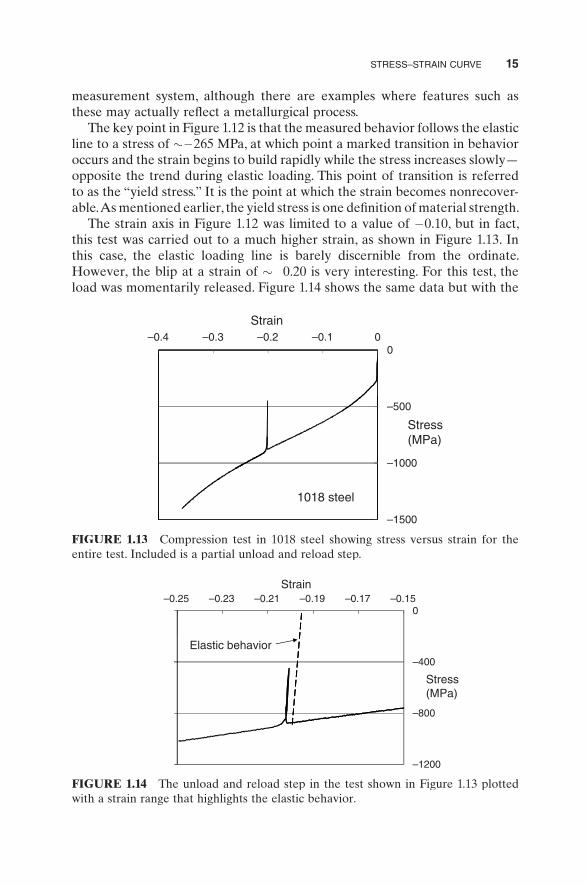
The strain axis in Figure 1.12 was limited to a value of − 0.10, but in fact,

this test was carried out to a much higher strain, as shown in Figure 1.13 . In

this case, the elastic loading line is barely discernible from the ordinate.

However, the blip at a strain of ∼− 0.20 is very interesting. For this test, the

load was momentarily released. Figure 1.14 shows the same data but with the

Strain

0–0.4 –0.3 –0.2 –0.1 0

–500

Stress(MPa)

–1000

1018 steel

–1500

FIGURE 1.13 Compression test in 1018 steel showing stress versus strain for the

entire test. Included is a partial unload and reload step.

FIGURE 1.14 The unload and reload step in the test shown in Figure 1.13 plotted

with a strain range that highlights the elastic behavior.

0–0.25 –0.23 –0.21 –0.19 –0.17 –0.15

Strain

–400

Stress

Elastic behavior

–800

(MPa)

–1200


x -axis adjusted to focus on the unloading/loading behavior. In Figure 1.14 , a

line with the slope of the elastic loading line has been drawn to illustrate that

the unloading/loading line follows the slope of the elastic line; that is, when

the load was decreased, the strain decreased along the elastic line rather than

along the solid line. And when the load was once again increased, the strain

increased along the elastic line until the previous maximum stress was reached.

At this point, the stress–strain curve followed the trend of the previous curve.

If the load had been decreased all the way to zero, then the strain would

have relaxed elastically by

εe

MPa

MPa= =

~

,. ,

875

212 0000 004

which is the maximum (absolute value of the) stress reached before unloading

divided by the elastic modulus. In the case of the compression test, the strain

is negative; thus, when the specimen is unloaded, it becomes less negative. The

permanent strain in the test specimen would have been

εep = − + = −0 202 0 004 0 198. . . ,

which is the maximum (negative) strain reached before unloading plus the

elastic strain that is recovered. The compression test specimen would have

been 19.8% shorter.

The strain past the yield stress has been referred to earlier as permanent

and nonrecoverable strain. The more traditional term is “plastic strain” as

opposed to “elastic strain” during the initial elastic portion of the loading cycle.

1.10 THE TRUE STRESS–TRUE STRAIN CONVERSION

Recall that all of the calculations of stress and strain have been based on the

initial cross-sectional area of the specimen (for the stress calculation) and

the initial length of the specimen (for the strain calculation). The specimen,

however, is deforming and the cross-sectional area changes. In a tension test,

the cross-sectional area decreases, whereas in a compression test, the area

increases. The stress–strain curves based on original dimension—as plotted in

Figure 1.13 —are referred to as “engineering” stress–strain curves. When the

stress during the test is based on the current (or actual) area and the strain is

based on the current length, the resulting curve is referred to as a “true” stress–

strain curve; that is, the incremental change in true strain, ε, is defi ned as

ddll

ε = , (1.10)

and the true strain , ε, in a test where the specimen ’ s length begins as Lo and

ends as Lf isf

THE TRUE STRESS–TRUE STRAIN CONVERSION 17

ε ε= = − =⎛⎝⎜⎜⎜

⎞⎠⎟⎟⎟ = +( )∫

dll

L LLL

L

L

o

f

f of

o

eln ln ln ln .1 (1.11)

The true strain is the logarithm of one plus the engineering strain. The true stress , σ, is defi ned asσ

σ =FA

,

where A is now taken as the current area:

σ σ= = =FA

AA

FA

AA

AA

o

o o

oe

o .

One distinction between elastic deformation and plastic deformation is that

whereas (as discussed in Section 1.7 ) volume is not conserved in the former,

it is conserved in the latter. Thus, plastic deformation is incompressible, and

σ σ σ σ ε= = = +( )eo

e

o

e e

AA

LL

1 . (1.12)

The true stress is simply the engineering stress multiplied by one plus the

engineering strain. Here the distinction between a tension test where εe is posi-

tive and a compression test where εe is negative becomes critically important.

For the compression test shown in Figure 1.13 , the conversion from an

engineering stress–strain curve to a true stress–strain curve yields the curve

shown in Figure 1.15 . Compare this curve with that in Figure 1.13 . The absolute

FIGURE 1.15 The stress–strain curve in Figure 1.13 (plotted as engineering stress

versus engineering strain) converted to true stress versus true strain.

0–0.50 –0.40 –0.30 –0.20 –0.10 0.00

True strain

–400

–200

–600

Truestress(MPa)

–1000

–800

1018 steel


value of the maximum stress is lower in the true stress–strain curve because

the diameter of the compression specimen increases during testing and the

force divided by the current area gives a smaller stress. The peak strain has

increased from ∼− 0.35 on engineering coordinates to ∼− 0.43 on true stress–

strain coordinates, which follows from ε = ln (1 − 0.35).

In this monograph, only true stress–strain properties will be considered.

However, engineers need to check to verify whether it is engineering or true

stress–strain curves that are being reported and to be explicit themselves when

reporting test results.

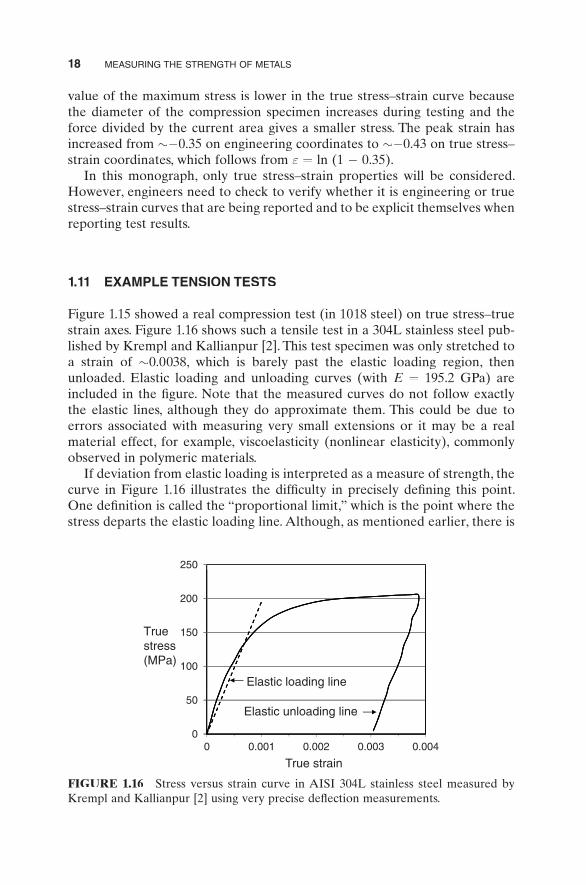
1.11 EXAMPLE TENSION TESTS

Figure 1.15 showed a real compression test (in 1018 steel) on true stress–true

strain axes. Figure 1.16 shows such a tensile test in a 304L stainless steel pub-

lished by Krempl and Kallianpur [2] . This test specimen was only stretched to

a strain of ∼0.0038, which is barely past the elastic loading region, then

unloaded. Elastic loading and unloading curves (with E = 195.2 GPa) are

included in the fi gure. Note that the measured curves do not follow exactly

the elastic lines, although they do approximate them. This could be due to

errors associated with measuring very small extensions or it may be a real

material effect, for example, viscoelasticity (nonlinear elasticity), commonly

observed in polymeric materials.

If deviation from elastic loading is interpreted as a measure of strength, the

curve in Figure 1.16 illustrates the diffi culty in precisely defi ning this point.

One defi nition is called the “proportional limit,” which is the point where the

stress departs the elastic loading line. Although, as mentioned earlier, there is

FIGURE 1.16 Stress versus strain curve in AISI 304L stainless steel measured by

Krempl and Kallianpur [2] using very precise defl ection measurements.

250

200

100

150Truestress(MPa)

Elastic loading line

0

50Elastic unloading line

0 0.001 0.002 0.003 0.004

True strain

EXAMPLE TENSION TESTS 19

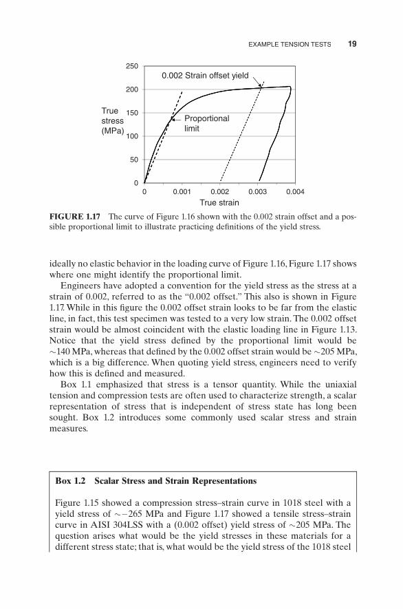
ideally no elastic behavior in the loading curve of Figure 1.16 , Figure 1.17 shows

where one might identify the proportional limit.

Engineers have adopted a convention for the yield stress as the stress at a

strain of 0.002, referred to as the “0.002 offset.” This also is shown in Figure

1.17 . While in this fi gure the 0.002 offset strain looks to be far from the elastic

line, in fact, this test specimen was tested to a very low strain. The 0.002 offset

strain would be almost coincident with the elastic loading line in Figure 1.13 .

Notice that the yield stress defi ned by the proportional limit would be

∼ 140 MPa, whereas that defi ned by the 0.002 offset strain would be ∼205 MPa,

which is a big difference. When quoting yield stress, engineers need to verify

how this is defi ned and measured.

Box 1.1 emphasized that stress is a tensor quantity. While the uniaxial

tension and compression tests are often used to characterize strength, a scalar

representation of stress that is independent of stress state has long been

sought. Box 1.2 introduces some commonly used scalar stress and strain

measures.

FIGURE 1.17 The curve of Figure 1.16 shown with the 0.002 strain offset and a pos-

sible proportional limit to illustrate practicing defi nitions of the yield stress.

250

200

True

0.002 Strain offset yield

100

150stress(MPa)

Proportionallimit

0

50

0.0010 0.002 0.003 0.004

True strain

Box 1.2 Scalar Stress and Strain Representations

Figure 1.15 showed a compression stress–strain curve in 1018 steel with a

yield stress of ∼−265 MPa and Figure 1.17 showed a tensile stress–strain

curve in AISI 304LSS with a (0.002 offset) yield stress of ∼ 205 MPa. The

question arises what would be the yield stresses in these materials for a

different stress state; that is, what would be the yield stress of the 1018 steel


in tension or torsion? There are two ways to consider this. The second will

be addressed in Box 3.4 in Chapter 3 .

The common model for the stress-state dependence of the yield stress is

based on the von Mises criterion. In the principal axis coordinate system,

J2JJ —the second invariant of the stress deviator—is

J2 1 22

2 32

3 121

6= −( ) + −( ) + −( )⎡

⎣⎤⎦σ σ σ σ σ σ ,

where J 2JJ is a scalar combination of the principal stresses. The von Mises

yield criterion states that yield occurs when J2JJ reaches the critical value

of k2 :

J k22= .

If σo is the yield stress in a tension test, where σ1 = σo and σ2 = σ3 = 0,

then

k =σo

3,

which defi nes the value of k. Note that due to the squared terms, the yield

stress in compression has the same absolute value as that in tension. In a

torsion test where σ1 = −σ2 = τ and τ σ3 = 0, then

J k

k

22

1 12

12

12

12

1

1

6

3 3

= = +( ) + +⎡⎣

⎤⎦ =

= = = =

σ σ σ σ σ

σ τσ

τσo o; .

Note that the yield stress in a torsion test is predicted to be 0.577, the

yield stress in uniaxial tension. The yield stress in tension σo is also referred

to as the von Mises stress, σv. Rearranging the above-mentioned equation v

defi ning J2JJ gives (for principal stress coordinate system)

σ σ σ σ σ σ σv = −( ) + −( ) + −( ){ }⎡

⎣⎢⎢

⎤

⎦⎥⎥

1

21 2

22 3

23 1

21 2

.

The von Mises strain (in principal axes) is defi ned as

ε ε ε ε ε ε εv = −( ) + −( ) + −( ){ }⎡

⎣⎢⎢

⎤

⎦⎥⎥

2

3

1

21 2

22 3

23 1

21 2

.

Recall in a tension test (with the tensile axis along the principal direction

“1”) that

EXAMPLE TENSION TESTS 21

ε εε

2 31

2= = − .

In this case, it can be shown that εv = ε1 ; the von Mises strain is equal to

the tensile strain.

For pure shear, ε1 = −ε3 = γ /2 and γγ ε2 = 0, where γ is the shear strain. Itγcan be shown that

pure shear v: .ε εγ

= =2

3 31

octa-hedral shear stress , τoctττ , defi ned as follows. Note the relation between this

scalar and the von Mises stress:

τ σ σ σoct v= = = =2

3

2

3

1

3

2

3

2

32

2J O O .

The octahedral shear strain, γoctγγ , is defi ned as

γ ε ε ε ε ε εoct = −( ) + −( ) + −( )⎡⎣

⎤⎦

2

31 2

22 3

23 1

2 1 2.

In a uniaxial tensile test, γoctγγ relates to the tensile strain ε1 through

γ εε ε

εε

oct = +⎛⎝⎜⎜⎜

⎞⎠⎟⎟⎟ + − −

⎛⎝⎜⎜⎜

⎞⎠⎟⎟⎟

⎡

⎣⎢⎢

⎤

⎦⎥⎥ =

2

3 2 2

2

3

31

12

11

2 1 2

112

12 1 2

12

1

2

3

2

2

3

9

2

⎛⎝⎜⎜⎜

⎞⎠⎟⎟⎟ + −

⎛⎝⎜⎜⎜

⎞⎠⎟⎟⎟

⎡

⎣⎢⎢

⎤

⎦⎥⎥ =

⎡

⎣⎢⎢

⎤

⎦⎥⎥

εε

22

12= ε .

Still another common scalar measure is the effective stress, σ :

σ σ σ σ σ σ σ= −( ) + −( ) + −( )⎡⎣

⎤⎦

2

21 2

22 3

23 1

2 1 2,

and the effective strain, ε :

ε ε ε ε ε ε ε= −( ) + −( ) + −( )⎡⎣

⎤⎦

2

31 2

22 3

23 1

2 1 2.

Both the effective stress and the effective strain reduce to the uniaxial

stress and strain, which is why the von Mises stress is often referred to as

the von Mises effective stress and, similarly, the von Mises strain is often

referred to as the von Mises effective strain.

While the von Mises yield criterion explicitly refers to yield, stress–strain

curves often plot the entire curve on von Mises stress and strain axes or

octahedral shear stress and strain axes.


1.12 ACCOUNTING FOR STRAIN MEASUREMENT ERRORS

The measurement of strain in a tension or compression specimen can be chal-

lenging. A defl ection measurement device such as that shown in Figure 1.4 is

costly and can be diffi cult to install—particularly when experiments at cryo-

genic temperatures or elevated temperatures are desired. One common prac-

tice is to use the linear variable displacement transducer ( LVDT ) attached to

the machine axis to record displacement in the test specimen, but as men-

tioned earlier, this measurement could represent displacements beyond those

in the test specimen. Recent development of noncontact strain measurement

devices based on laser interferometry offers an attractive alternative [3] . Even

these new techniques, though, can introduce measurement artifacts. Thus,

when viewing stress–strain measurements in the published literature, one

must be cognizant of potential effects of errors in the strain measurement

system.

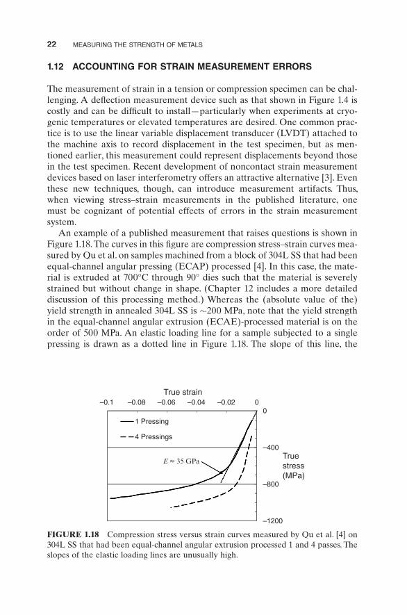
An example of a published measurement that raises questions is shown in

Figure 1.18 . The curves in this fi gure are compression stress–strain curves mea-

sured by Qu et al. on samples machined from a block of 304L SS that had been

equal-channel angular pressing ( ECAP ) processed [4] . In this case, the mate-

rial is extruded at 700°C through 90° dies such that the material is severely

strained but without change in shape. (Chapter 12 includes a more detailed

discussion of this processing method.) Whereas the (absolute value of the)

yield strength in annealed 304L SS is ∼ 200 MPa, note that the yield strength

in the equal-channel angular extrusion (ECAE)-processed material is on the

order of 500 MPa. An elastic loading line for a sample subjected to a single

pressing is drawn as a dotted line in Figure 1.18 . The slope of this line, the

FIGURE 1.18 Compression stress versus strain curves measured by Qu et al. [4] on

304L SS that had been equal-channel angular extrusion processed 1 and 4 passes. The

slopes of the elastic loading lines are unusually high.

0–0.1 –0.08 –0.06 –0.04 –0.02 0

1 Pressing

True strain

–400

4 Pressings

E ≈ 35 GPaTrue

–800

stress(MPa)

–1200

ACCOUNTING FOR STRAIN MEASUREMENT ERRORS 23

apparent elastic modulus, is ∼35 MPa. The typical elastic modulus of stainless

steels, however, is ∼192 MPa. Since strain alone—even high levels of strain

produced by ECAP processing—does not alter the interatomic forces, the

apparent modulus must either be an artifact of the strain measurement or

refl ect unusual loading behavior.

Although in this case Qu et al. are confi dent that the strain measurements

reported by them are accurate and that the low initial slope is real * (perhaps

indicating microplasticity in a few grains), this measurement serves as an

example of the effect of a measurement system that indicates displacements

beyond actual elastic displacements in the deforming specimen.

To illustrate the issue, Figure 1.19 is a schematic two-spring system, which

is a model for the elastic displacements of a mechanical test specimen attached

to a load frame. In this model, the test specimen has a spring constant (equiva-

lent to an elastic modulus) of E1, whereas the load frame has a spring constant

of E2, which is assumed to be a constant. A force F is applied to the load axis Fand the total displacement, ΔY , is measured with an LVDT. In this case, theYYtotal displacement is

ΔYFE

FE

= +1 2

(1.13)

* This was communicated in a private conversation with a member of the Qu et al. research group.

FIGURE 1.19 Schematic spring analogy illustrating how the stiffness (elastic

modulus) of the machine can add to displacements measuring using an LVDT.

Spring constant (elastic

modulus) of the test E1

specimen

Spring constant (elastic modulus) of the machineE2

ΔY

frame

LVDT Measures ΔY

F


and the displacement within the test specimen is

Δ ΔY YFE

1

2

= − . (1.14)

If the displacements within the machine frame are not subtracted from the

total displacements, the (absolute value of the) presumed displacements within

the test specimen will be too large. Once the test specimen begins to plastically

deform, the elastic displacements within the machine frame will continue to

add to the measured displacements. Inaccurate measurement of displacements

within the test specimen offers one source of error in the stress–strain curve.

This error compounds in the true stress calculation using Equation (1.12)

since the conversion from engineering to true stress involves multiplication of

the engineering stress by (1 + e ), which relies on an accurate measurement of

the engineering strain using Equation (1.4) .

Fortunately, a simple correction is possible under certain idealized condi-

tions. When, for instance, the machine modulus is constant and the errors to

the measurement of strain solely arise from displacements in the machine

frame, the fi ctitious elastic displacements (engineering strains) can be sub-

tracted from the measured displacements. *

In this case, the actual elastic strains can be computed using the known

specimen modulus:

ε εσ σ

e ee

app

e

actact app= − +

E E, (1.15)

where the subscript “app” refers to “apparent” and “act” refers to “actual.”

Note that the correction is performed on the engineering values of stress and

strain and that the signage is very important.

Figure 1.20 shows the stress–strain curves from Figure 1.18 corrected using

Equation (1.15) . In this case, the actual measured apparent moduli for the 1-pass

and 4-pass curves are used. As indicated in Figure 1.18 , this was 35 GPa for the

1-pass curve and 74 GPa for the 4-pass curve. The actual modulus was assumed

to equal 192 GPa for both cases. A comparison between the raw data in Figure

1.18 and the corrected curves in Figure 1.20 shows that it is mostly the strain

values that have changed. The stresses show less of a change since the strains

in these tests were fairly low (compared, for instance, with those in Figure 1.13

and Figure 1.15 ) It is worth reemphasizing that Qu et al. believe that the strains

are accurate, in which case the stress–strain curves in Figure 1.18 are accurate

and there is no reason to apply the above-mentioned correction. It is done only

* The fact that the slopes of the elastic portions of the 1-pressing and 4-pressing curves are not

identical suggests that the high slope does not simply arise from a machine compliance effect.

Assuming a constant machine modulus, thus, is an approximation.

FORMATION OF A NECK IN A TENSILE SPECIMEN 25

as an illustration. For tests carried to large strains, the errors introduced by

inaccurate strain measurements can be signifi cant.

1.13 FORMATION OF A NECK IN A TENSILE SPECIMEN

Figure 1.21 shows another tensile test measurement. This one was reported by

Antoun [5] and is also in a 304 stainless steel—but at 160°F instead of room

temperature. This stress–strain curve was taken all the way to a true strain of

FIGURE 1.20 True stress versus true strain curves from Figure 1.18 with apparent

elastic strains not associated with those in the test specimen removed using Equation

(1.15) .

0–0.08 –0.06 –0.04 –0.02 0

1 Pressing

True strain

–400

4 Pressings

True

–800

stress(MPa)

–1200

FIGURE 1.21 Stress versus strain (tension) measured in 304 SS by Antoun [5] at

160°F (71°C).

100

120

60

80True stress(MPa)

20

40

160°F

00 0.1 0.2 0.3 0.4 0.5

True strain


∼ 0.44. The unloading portion of the curve (as load is reduced to zero) is not

shown. It is likely that this test specimen formed a neck and broke (as in Figure

1.9 ).

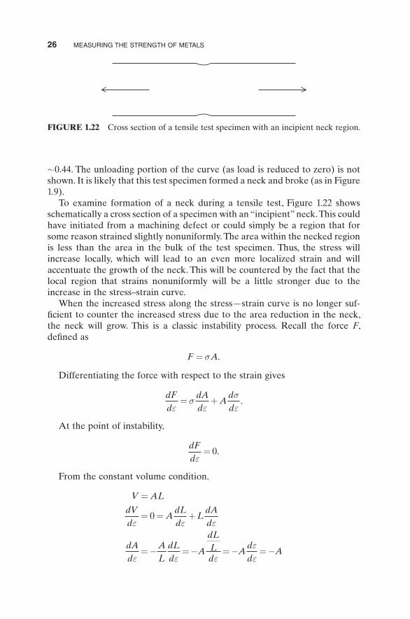
To examine formation of a neck during a tensile test, Figure 1.22 shows

schematically a cross section of a specimen with an “incipient” neck. This could

have initiated from a machining defect or could simply be a region that for

some reason strained slightly nonuniformly. The area within the necked region

is less than the area in the bulk of the test specimen. Thus, the stress will

increase locally, which will lead to an even more localized strain and will

accentuate the growth of the neck. This will be countered by the fact that the

local region that strains nonuniformly will be a little stronger due to the

increase in the stress–strain curve.

When the increased stress along the stress—strain curve is no longer suf-

fi cient to counter the increased stress due to the area reduction in the neck,

the neck will grow. This is a classic instability process. Recall the force F , FFdefi ned as

F A= σ .

Differentiating the force with respect to the strain gives

dFd

dAd

Addε

σε

σε

= + .

At the point of instability,

dFdε

= 0.

From the constant volume condition,

V AL

dVd

AdLd

LdAd

dAd

AL

dLd

A

dLLd

Add

A

=

= = +

= − = − = − = −

ε ε ε

ε ε εεε

0

FIGURE 1.22 Cross section of a tensile test specimen with an incipient neck region.

STRAIN RATE 27

dFd

dAd

Add

A Addε

σε

σε

σσε

= = + = − +0 .

Therefore, at the point of instability,

σσε

=dd

. (1.16)

When the true stress equals the slope of the true stress versus true strain

curve, the specimen is prone to undergoing unstable deformation via forma-

tion of a neck. The instability condition represented by Equation (1.16) is

referred to as the Considère criterion in recognition of the 1885 experimental

observations in iron and steel by this French researcher. Figure 1.23 shows the

stress–strain data of Figure 1.21 plotted along with dσ /σ dε . Recall that since εis dimensionless, dσ /σ dε has the units of stress.

The two curves in Figure 1.23 coincide at a strain of ∼0.41. Thus, per the

instability condition, a neck likely begins to form at this point and the tensile

specimen will soon break. In addition, data are not reported past this point

since the stress and strain are no longer uniform in the test specimen. This

prediction is consistent with the measurement shown in Figure 1.21 .

1.14 STRAIN RATE

In the test results highlighted in Figure 1.13 , Figure 1.16 , Figure 1.18 , and Figure

1.21 , the velocity of the crosshead has not been specifi ed. This actually is an

important variable. Typically, the yield stress in a test where the cross-head

FIGURE 1.23 Strain hardening rate (slope of the stress–strain curve) versus true

stress for the tensile test shown in Figure 1.21 . The point of intersection of these curves

is the point of tensile instability.

2000

dd

1000

1500

MPa

0

500

True stress

00 0.1 0.2 0.3 0.4 0.5

True strain

σ ε


velocity is high exceeds that in a test where the crosshead is low. The difference

can be small, but it is generally measureable.

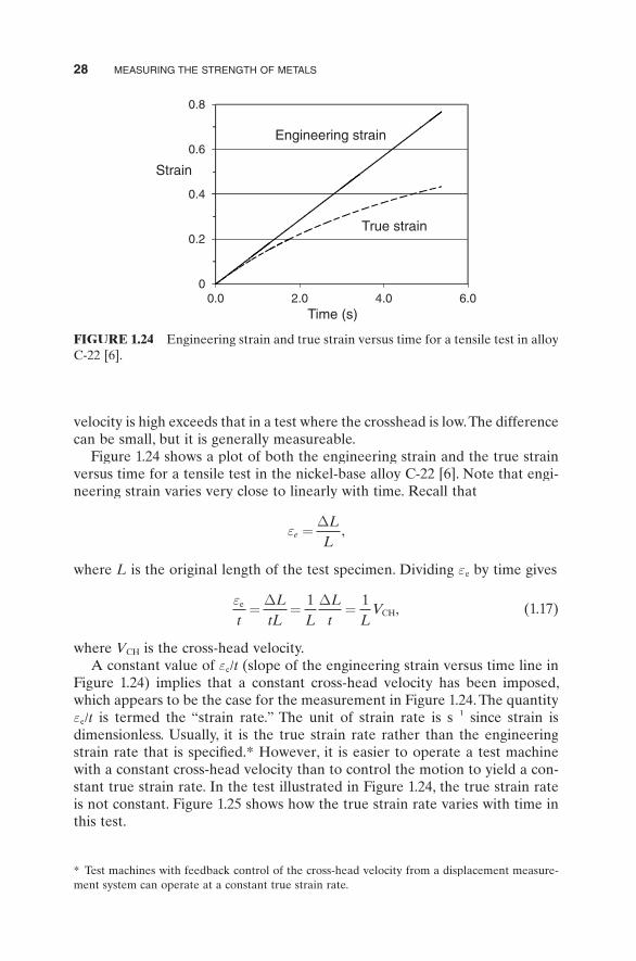
Figure 1.24 shows a plot of both the engineering strain and the true strain

versus time for a tensile test in the nickel-base alloy C-22 [6] . Note that engi-

neering strain varies very close to linearly with time. Recall that

εeL

L=

Δ,

where L is the original length of the test specimen. Dividing εe by time gives

εeCH

tL

tL LLt L

V= = =Δ Δ1 1

, (1.17)

where VCHVV is the cross-head velocity.

A constant value of εe/ t (slope of the engineering strain versus time line in tFigure 1.24 ) implies that a constant cross-head velocity has been imposed,

which appears to be the case for the measurement in Figure 1.24 . The quantity

εe /t is termed the “strain rate.” The unit of strain rate is st − 1 since strain is

dimensionless. Usually, it is the true strain rate rather than the engineering

strain rate that is specifi ed. * However, it is easier to operate a test machine

with a constant cross-head velocity than to control the motion to yield a con-

stant true strain rate. In the test illustrated in Figure 1.24 , the true strain rate

is not constant. Figure 1.25 shows how the true strain rate varies with time in

this test.

FIGURE 1.24 Engineering strain and true strain versus time for a tensile test in alloy

C-22 [6] .

0.8

0.6Engineering strain

Strain

0.2

0.4

True strain

00.0 2.0 4.0 6.0

Time (s)

* Test machines with feedback control of the cross-head velocity from a displacement measure-

ment system can operate at a constant true strain rate.

EXERCISES 29

The true strain rate for this test started at a value nearly equal 0.14 s−1 at

yield but decreased throughout the test. The average true strain rate was

approximately equal to 0.08 s−1 .

1.15 MEASURING STRENGTH: SUMMARY

The mechanical test is used to measure the strength of materials. This chapter

has reviewed the tensile test; introduced defi nitions of stress, strain, and strain

rate; discussed elastic and plastic deformation; and summarized concepts such

as compressibility, instability, and errors introduced by imprecise displacement

measurement. Several examples of stress–strain curves—in tension as well as

compression—have been presented. With this introduction, the contributions

to the strength measured in a mechanical test can be presented.

EXERCISES

1.1 A copper tensile test specimen is machined with an initial diameter of

5.00 mm and an initial gage length of 40.0 mm. A load of 400 N is

applied.

(a) At this load, what is the applied stress?

(b) If the specimen only deforms elastically, calculate the defl ection

that would be measured.

1.2 Measurements of load versus defl ection in a metallic tensile test speci-

men with an initial diameter of 6.00 mm and an initial gage length of

50.0 mm are given in the following table.

(a) Does this specimen appear to be deforming elastically?

(b) From the elastic constants in Table E1.2 , determine the metal.

FIGURE 1.25 True strain rate versus time for the alloy C-22 tensile test (slope of the

true strain versus time curve in Figure 1.24 ).

0.16

0.12

True strain

0 04

0.08rate (s–1)

0.000.0 2.0 4.0 6.0

Time (s)


1.3 An Al2O 3 solid cylinder with an initial length of 1.50 cm and an initial

diameter of 1.00 cm is loaded in compression. An optical extensometer

is used that continuously measures the diameter of the test specimen.

Table E1.3 lists the measured force versus diameter. Assuming that Pois-

son ’ s ratio for this material is 0.25, compare the elastic modulus with the

value listed in Table 1.2 . (Note that the forces are listed as negative to

refl ect the compressive loading.)

TABLE E1.3

ΔD (μ m) Force (N)

0.36 − 3,9601.81 −19,6003.26 −35,3004.71 −51,0006.16 −66,8007.61 −82,4009.06 −98,200

10.51 −113,800

TABLE E1.2

ΔL (μ m) Force (N)

5.4 57216.2 166226.9 280737.6 392148.4 508959.2 618969.9 732680.7 8457

1.4 Compare the forces required to perform the tensile test in Exercise 1.2

with the forces required to perform the compression test in Exercise 1.3.

Instron ® and MTS® are two companies that supply mechanical testing

machines. Go to either the Instron or MTS website and research which

testing machine would be required to perform these mechanical tests.

1.5 A copper tensile test specimen is machined with an initial diameter of

5.00 mm and an initial gage length of 40.0 mm. The measured load (N)

versus displacement ( μm) data is listed in Table E1.5 .

(a) Calculate and plot stress versus strain for this test.

(b) Has the yield stress been exceeded in this test?

EXERCISES 31

1.6 For the test described in Exercise 1.5,

(a) estimate the proportional limit and

(b) estimate the 0.002 offset yield stress.

1.7 The test described in Exercise 1.5 was actually strained to a higher total

elongation. Table E1.7 lists the measured elongation versus force data.

Add these data to the data listed in Exercise 1.5.

(a) Plot the engineering stress–strain curve.

(b) Calculate and plot the true stress–strain curve. (Remember that

the conversion from engineering strain and stress to true strain and

stress needs to be performed only for points beyond the yield

stress.)

TABLE E1.5

ΔL (μ m) Force (N)

4.1 2697.9 532

12 81316 106819.2 123124 156028.1 181731.9 197336.1 210840.4 219548.1 240756.1 258364.1 274072.2 290380 310488.3 318295.9 3368

112.2 3659128.2 3845144.3 4141160.3 4289176.5 4507


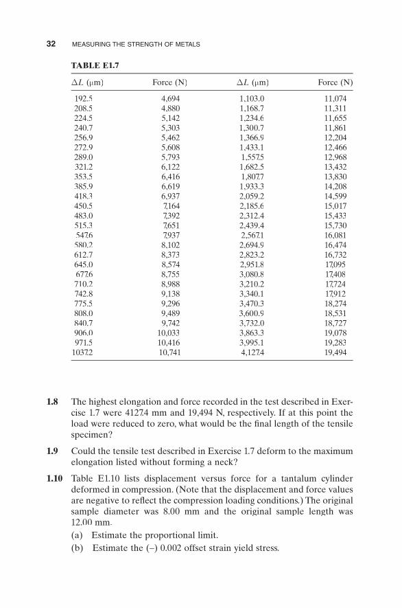
1.8 The highest elongation and force recorded in the test described in Exer-

cise 1.7 were 4127.4 mm and 19,494 N, respectively. If at this point the

load were reduced to zero, what would be the fi nal length of the tensile

specimen?

1.9 Could the tensile test described in Exercise 1.7 deform to the maximum

elongation listed without forming a neck?

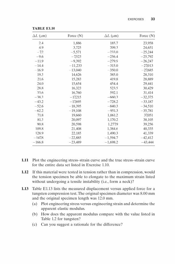
1.10 Table E1.10 lists displacement versus force for a tantalum cylinder

deformed in compression. (Note that the displacement and force values

are negative to refl ect the compression loading conditions.) The original

sample diameter was 8.00 mm and the original sample length was

12.00 mm.

(a) Estimate the proportional limit.

(b) Estimate the (–) 0.002 offset strain yield stress.

TABLE E1.7

ΔL (μ m) Force (N) ΔL (μ m) Force (N)

192.5 4,694 1,103.0 11,074208.5 4,880 1,168.7 11,311224.5 5,142 1,234.6 11,655240.7 5,303 1,300.7 11,861256.9 5,462 1,366.9 12,204272.9 5,608 1,433.1 12,466289.0 5,793 1,557.5 12,968321.2 6,122 1,682.5 13,432353.5 6,416 1,807.7 13,830385.9 6,619 1,933.3 14,208418.3 6,937 2,059.2 14,599450.5 7,164 2,185.6 15,017483.0 7,392 2,312.4 15,433515.3 7,651 2,439.4 15,730547.6 7,937 2,567.1 16,081580.2 8,102 2,694.9 16,474612.7 8,373 2,823.2 16,732645.0 8,574 2,951.8 17,095677.6 8,755 3,080.8 17,408710.2 8,988 3,210.2 17,724742.8 9,138 3,340.1 17,912775.5 9,296 3,470.3 18,274808.0 9,489 3,600.9 18,531840.7 9,742 3,732.0 18,727906.0 10,033 3,863.3 19,078971.5 10,416 3,995.1 19,283

1037.2 10,741 4,127.4 19,494

EXERCISES 33

TABLE E1.10

ΔL (μ m) Force (N) ΔL ( μm) Force (N)

−2.4 − 1,886 −185.7 − 23,958

−4.9 − 3,725 −209.3 − 24,651

−7.2 − 5,571 −233.0 − 25,244

−9.6 − 7,523 −256.4 − 25,792

− 11.9 − 9,392 −279.9 − 26,247

−14.4 − 11,233 −315.0 −27,013

−16.9 − 13,040 −350.0 − 27,685

−19.3 − 14,626 −385.0 − 28,310

− 21.6 − 15,283 −419.8 − 28,889

− 24.0 − 15,654 −454.4 − 29,441

− 28.8 − 16,323 −523.5 − 30,429

− 33.6 − 16,760 −592.1 − 31,414

− 38.3 − 17,215 −660.3 − 32,375

− 43.2 − 17,695 −728.2 − 33,187

− 52.6 − 18,395 −840.3 − 34,510

− 62.2 − 19,108 −951.3 − 35,781

− 71.8 − 19,660 − 1,061.2 − 37,051

− 81.3 − 20,097 −1,170.2 − 38,105

− 90.8 − 20,598 −1,277.9 − 39,256

−109.8 − 21,408 −1,384.6 − 40,335

−128.9 − 22,185 −1,490.3 − 41,339

− 147.8 − 22,885 −1,594.7 − 42,412

− 166.8 − 23,489 −1,698.2 −43,444

1.11 Plot the engineering stress–strain curve and the true stress–strain curve

for the entire data set listed in Exercise 1.10.

1.12 If this material were tested in tension rather than in compression, would

the tension specimen be able to elongate to the maximum strain listed

without undergoing a tensile instability (i.e., form a neck)?

1.13 Table E1.13 lists the measured displacement versus applied force for a

tungsten compression test. The original specimen diameter was 8.00 mm

and the original specimen length was 12.0 mm.

(a) Plot engineering stress versus engineering strain and determine the

apparent elastic modulus.

(b) How does the apparent modulus compare with the value listed in

Table 1.2 for tungsten?

(c) Can you suggest a rationale for the difference?


TABLE E1.13

ΔL (μ m) Force (N) ΔL ( μ m) Force (N)

–23.8 –3,916 –528.9 –75,442–47.7 –8,170 –575.4 –76,089–71.6 –12,216 –624.1 –76,656–95.4 –15,890 –672.1 –77,415

–119.9 –20,134 –719.5 –77,703–145.0 –23,989 –767.3 –78,266–167.5 –28,082 –815.3 –78,835–192.2 –32,012 –864.5 –79,343–216.8 –36,201 –912.4 –79,574–239.3 –40,076 –959.6 –80,102–264.7 –44,121 –1,007.5 –80,259–287.5 –48,382 –1,055.1 –80,934–312.9 –52,415 –1,104.8 –80,983–335.4 –56,339 –1,152.7 –81,591–360.1 –60,182 –1,200.1 –81,797–384.7 –64,281 –1,248.9 –82,345–407.8 –68,243 –1,295.7 –82,626–432.2 –71,999 –1,343.1 –82,794–480.5 –73,694 –1,391.6 –83,012

1.14 Assuming that the true elastic modulus is 411 MPa, perform a correction

to remove the artifi cial elastic strain. Compare the corrected and uncor-

rected engineering stress–strain curves.

1.15 Table E1.15 lists the measured displacement versus time for a tensile

test on a specimen with an initial length of 25.0 mm.

(a) Plot the engineering strain versus time and the true strain versus

time.

(b) Was this test run at a uniform engineering strain rate or a uniform

true strain rate?

(c) What is this strain rate?

REFERENCES 35

TABLE E1.15

Time (s) ΔL ( μm) Time (s) ΔL ( μm)

2.93 0.070 104.79 2.7588.83 0.216 111.17 2.942

14.99 0.372 116.71 3.09820.96 0.527 123.12 3.28127.2 0.674 129.07 3.43832.79 0.846 134.75 3.61039.09 0.987 141.21 3.78545.1 1.161 146.88 3.96150.87 1.298 153.27 4.12957.19 1.457 159.04 4.29862.85 1.619 165.08 4.49568.88 1.786 171.22 4.66274.93 1.943 177.03 4.84480.88 2.105 182.97 5.02686.8 2.265 189.16 5.19592.76 2.444 195.1 5.37898.71 2.604 201.08 5.557

REFERENCES

1 G.T. Gray III and S.R. Chen , “ MST-8 constitutive properties & constitutive model-

ing ,” Los Alamos National Laboratory, LA_CP-07-1590 and LA-CP-03-006, 2007 .

2 E. Krempl and V.V. Kallianpur , “ Some critical uniaxial experiments for viscoplastic-

ity at room temperature ,” Journal of the Mechanics and Physics of Solids , Vol. 32 ,

No. 4 , 1984 , p. 301 .

3 B. Becker and M. Dripke , “ Choosing the right extensometer for every materials

testing application ,” Advanced Materials & Processes , Vol. 169 , No. 4 , 2011 , pp.

17 – 21 .

4 S. Qu , C.X. Huang , Y.L. Gao , G. Yang , S.D. Wu , Q.S. Zang , and Z.F. Zhang , “ Tensile

and compressive properties of AISI 304L stainless steel subjected to equal channel

angular pressing ,” Materials Science and Engineering A , Vol. 475 , 2008 , pp.

207 – 216 .

5 B.R. Antoun , “ Temperature effects on the mechanical properties of annealed and

HERF 304L stainless steel ,” Sandia National Laboratories, Sandia Report,

SAND2004-3090, November 2004 .

6 B.O. Tolle , “ Identifi cation of dynamic properties of materials for the nuclear waste

package ,” Technical Report, Task 24, Document ID: TR-02-007, September 2003 .

See Task 24 documents at the following website: http://hrcweb.nevada.edu/data/tda/

(accessed April 2011 ).

measuring the strength of metalsmedia.public.gr/books-pdf/9781118413418-0831211.pdf · 2 measuring...

Documents