measuring the distance between mer ge t...

Measuring the Distance between Merge Trees

Kenes Beketayev, Damir Yeliussizov, Dmitriy Morozov, Gunther H. Weber, andBernd Hamann

Abstract Merge trees represent the topology of scalar functions. To assess the topo-logical similarity of functions, one can compare their merge trees. To do so, oneneeds a notion of a distance between merge trees, which we define. We provideexamples of using our merge tree distance and compare this new measure to otherways used to characterize topological similarity (bottleneck distance for persistencediagrams) and numerical difference (L∞-norm of the difference between functions).

Kenes BeketayevLawrence Berkeley National Laboratory, One Cyclotron Rd, Berkeley, CA 94720, USANazarbayev University, 53 Kabanbay Batyr Ave, Astana, Kazakhstan, 010000e-mail: [email protected]

Damir YeliussizovKazakh-British Technical University, 59 Tole Bi St, Almaty, Kazakhstan, 050000e-mail: [email protected]

Dmitriy MorozovLawrence Berkeley National Laboratory, One Cyclotron Rd, Berkeley, CA 94720, USAe-mail: [email protected]

Gunther H. WeberLawrence Berkeley National Laboratory, One Cyclotron Rd, Berkeley, CA 94720, USAInstitute for Data Analysis and Visualization (IDAV), Department of Computer Science, Universityof California, Davis, CA 95616-8562, USAe-mail: [email protected]

Bernd HamannInstitute for Data Analysis and Visualization (IDAV), Department of Computer Science, Universityof California, Davis, CA 95616-8562, USAe-mail: [email protected]

1

2 Kenes Beketayev et al.

1 Introduction

Many aspects of physical phenomena are described and modeled by scalar func-tions. Computational and experimental capabilities allow us to approximate scalarfunctions at increasing levels of detail and resolution. This fact makes it necessaryto analyze and also compare such function automatically, when possible, and to in-clude more abstract analysis methods. Topological methods, based on the character-ization of a scalar function via its critical point behavior, are gaining in importance,and we were therefore motivated to investigate the feasibility of comparing scalarfunctions using their topological similarity. Computational chemistry, physics andclimate sciences are just a few applications where our ideas presented here shouldbe valuable.

We address the generic problem of comparing the topology of scalar functions.Fig. 1 demonstrates this problem. The figure shows slightly shifted versions of thesame function, colored red and blue. Commonly used analytical distances (e.g.,norms of the difference) between these functions would result in a non-zero value,failing to highlight the fact that they have the same sub-level set topology.

Scalar Functions Persistence Diagrams

Fig. 1 Consider two scalar functions, where one is a slightly shifted version of theother. Comparing them directly, e.g., via the L∞ norm, results in a large difference.Their persistence diagrams are the same, thus capturing the topological similarity ofthese functions.

One well-established distance that expresses the topological similarity in theabove example is the bottleneck distance between persistence diagrams, introducedby Cohen-Steiner et al. [8]. Computing the bottleneck distance for the example inFig. 1 results in zero. Originally motivated by the shape matching problem, wherethe goal is to find how similar shapes are based on similarity of their topology, thebottleneck distance also has an important property — robustness to noise; see Fig. 2.

However, the bottleneck distance does not incorporate sub-level set nesting in-formation, often necessary for analysis. Fig. 3 shows two functions that differ by thenesting of the maximum m. The bottleneck distance between the corresponding per-sistence diagrams is again zero. Nevertheless, the corresponding merge trees cannotbe matched exactly, hinting at a positive difference.

To resolve this problem, we introduce a new definition of the distance betweenmerge trees. This distance resembles the bottleneck distance between the persistencediagrams of sub-level sets of the function, but it also respects the nesting relationship

Measuring the Distance between Merge Trees 3

Fig. 2 Consider two close scalar functions on the left, where one contains additionalnoise. If we construct their persistence diagrams and find the bottleneck distance(which corresponds to the longest black line segment between paired points on theright), the result is small, correctly reflecting the closeness of the functions. In fact,the difference is the same as the level of the noise, which in this example is small.

Scalar Functions Merge Trees Persistence Diagrams

m m m m

Fig. 3 Consider two scalar functions on the left. The bottleneck distance betweenpersistence diagrams on the right equals zero, as points of two diagrams overlap.However, comparing the corresponding merge trees reveals a difference, since wecannot match them exactly. This difference highlights existence of additional nest-ing information in merge trees. Quantifying it is the main goal of this work.

between sub-level sets. Furthermore, the proposed distance implicitly distinguishesthe noise in the data, similar to the bottleneck distance, resulting in robust measure-ments resilient to perturbations of the input. This property is crucial when workingwith scientific data, where noise is a serious problem for any analysis.

The main contributions of this chapter are: a definition and an algorithm for com-puting the distance between merge trees; computation of the number of branch de-compositions of the merge tree; an experimental comparison between the proposeddistance, the bottleneck distance, and the L∞ norm on analytical and real-world datasets.

Sect. 2 presents related work and background in scalar field topology, persistenthomology, graph theory, and shape matching. Sect. 3 provides the definition andthe algorithm for computing the distance between merge trees. Sect. 4 demonstratesseveral use cases and presents the results of comparing the distance between mergetrees to the bottleneck distance between persistence diagrams, as well as the L∞norm. Finally, Sect. 5 summarizes the work and suggests ideas for future work.


2 Related Work

2.1 Scalar Field Topology

Scalar field topology characterizes data by topological changes of its level sets.Given a smooth, real-valued function without degenerate critical points, level settopology changes only at isolated critical points [16]. Several structures relate criti-cal points to each other.

The contour tree [5, 7] and the Reeb graph [21, 20] track the level sets of thefunction by recording their births (at minima), merges or splits (at saddles), anddeaths (at maxima). The contour tree is a special case of the Reeb graph, as thelatter permits loops in the graph to handle holes in the domain. Both structures areused in a variety of high-dimensional scalar field visualization techniques [23, 18].

Alternatively, the Morse–Smale complex [10, 9] segments the function into theregions of uniform gradient flow and encodes geometric information. It is also usedfor analysis of high-dimensional scalar functions [12].

We focus on a structure called merge tree (sometimes called a barrier tree [11,13]), as it tracks the evolution of sub-/super-level sets, while still being related tothe level-set topology through critical points [16].

2.2 Persistent Homology

The concept of homology in algebraic topology offers an approach to studying thetopology of the sub-level sets. We refer to Munkres [17] for the detailed introductionto homology. Informally, it describes the cycles in a topological space: the numberof components, loops, voids, and so on. We are only interested in 0–dimensionalcycles, i.e., the connected components.

Persistent homology tracks changes to the connected components in sub-levelsets of a scalar function. We say that a component is born in the sub-level setf−1(−∞,b] when its homology class does not exist in any sub-level set f−1(−∞,b−ε]. This class dies in the sub-level set f−1(∞,d] if its homology class merges withanother class that exists in a sub-level set f−1(−∞,b′] with b′ < b. When a com-ponent is born at b and dies at d, we record a pair (b,d) in the (0–dimensional)persistence diagram of the function f , denoted D( f ). For technical reasons, we addto D( f ) infinitely many copies of every point (a,a) on the diagonal.

Persistence diagrams reflect the importance of topological features of the func-tion: the larger the difference d−b of any point, the more we would have to changethe function to eliminate the underlying feature. Thus, persistence diagrams let usdistinguish between real features in the data and noise.

In Cohen-Steiner et al. [8], the authors prove the stability of persistence diagramswith respect to the bottleneck distance, dB(D( f ),D(g)). This distance is defined asthe infimum over all bijections, γ : D( f )→ D(g), of the largest distance between the


corresponding points,

dB(D( f ),D(g)) = infγ

supu∈D( f )

||u− γ(u)||∞.

Their result guarantees that the bottleneck distance is bounded by the infinity normbetween functions:

dB(D( f ),D(g))≤ ‖ f −g‖∞.

We use the bottleneck distance between persistence diagrams as a comparisonbaseline for the distance between merge trees.

2.3 Distance between Graphs

Graph theory offers several approaches for comparing graphs and defining a notionof a distance between them.

A common approach for measuring a distance between graphs is based on anedit distance. It is computed as a number of edit operations (add, delete, and swapin the case of a labeled graph) required to match two graphs [6], or, in a spe-cial case, trees [4]. The edit distance focuses on finding an isomorphism betweengraphs/subgraphs, while for merge trees we can have two isomorphic trees with apositive distance (see the example in Fig. 3).

Alternatively, in a specific case of rooted trees, one can consider the generalizedtree alignment distance [15], which, in addition to the edit distance, considers theminimization of the sum of distances between labeled end-points of any edge intrees. However, it is not clear how to adapt this distance definition for our purposes.

2.4 Using Topology of Real Functions for Shape Matching

The field of shape matching offers several methods related to our work. Generally,these methods focus on developing topological descriptors by treating a shape as amanifold, defining some real function on that manifold, and computing topologicalproperties of the function. The selection of the particular function usually dependson which specific topological and shape properties of interest [2].

While the majority of the mentioned descriptors are not directly related to ourwork, two topological descriptors use similar approaches in defining a similaritymeasure. One is called a multiresultion Reeb graph, proposed by Hilaga et al. [14],which encodes nesting information into nodes of a Reeb graph for different hierar-chy resolutions. Here, the hierarchy is defined by the simplification of Reeb graph.Another descriptor is based on an extended Reeb graph (ERG), proposed by Biasottiet al. [3]. It starts by computing the ERG of the underlying shape, which is basicallya Reeb graph with encoded quotient spaces in its vertices. It couples various geo-


metric attributes with the ERG, resulting in an informative topological descriptor. Inboth cases, similarity of shapes is measured by applying a specialized graph match-ing (based on embedded/coupled information) to descriptors. However, we focusonly on the sub-level set topology information, and design a matching algorithm,tailored specifically for this case.

Thomas and Natarajan [22] focus on symmetry discovery in a scalar functionbased on its contour tree. The authors develop a similarity measure between sub-trees of the contour tree, which in some regards is similar to our proposed measure.However, they consider a single pre-processed branch decomposition, and focus ondiscovering symmetry in a sole function.

3 Defining a Distance Between Merge Trees

In this section, we provide a formal definition of the distance between merge treesand provide an algorithm (with optimizations) for computing it. In short, to com-pute the distance between two merge trees, we consider all branch decompositionsof both trees and try to find a pair that minimizes the matching cost between them.Additionally, we provide the details of computing the number of branch decompo-sitions of a merge tree, used in complexity analysis of our algorithm.

3.1 Definition

Let K be a simplicial complex; let f : K → R be a continuous piecewise-linearfunction, defined on the vertices and interpolated in the interior of the simplices.Furthermore, assume all vertices have unique function values; in practice, we cansimulate this by breaking ties lexicographically.

Let Tf be a merge tree of the function f ; every vertex of K is mapped to a vertexin the merge tree. Every vertex of the merge tree has a degree of either one, two, ormore, corresponding to a minimum, a regular point, or a merge saddle. Our defini-tion works for higher-dimensional saddles (degenerate critical points) as well, andthey need explicit consideration only in the complexity analysis of the algorithm(Sect. 3.4). A merge tree with purged regular vertices is called reduced.

A branch decomposition B [19] of a reduced merge tree T is a pairing of allminima and saddles such that for each pair there exists at least one descending pathfrom the saddle to the minimum. We consider a rooted tree representation R of thebranch decomposition B, such that the rooted tree representation R is obtained bytranslating each branch b = (m,s) ∈ B into a vertex v ∈ R, where m and s are mini-mum and saddle that form the branch b. The edges of the rooted tree representationdescribe parent–child relationships between branches, see Fig. 4.


Given two merge trees, Tf and Tg, consider all their possible branch decompo-sitions, BTf = {R f

1 , ...,Rfk} and BTg = {Rg

1, ...,Rgk}, respectively; see Fig. 4.We need

two auxiliary definitions to describe the matching of rooted branch decompositions.

f

a

bc

d

e

a a a

e e e

d d d

c c cb b b

g

a

b

d

e

c

a a a

e e e

d d d

c c cb b b

(a, e)

(b, e) (c, d)

(c, e)

(a, d) (b, e)

(b, e)

(a, e)

(c, d)

(a, e)

(b, e)

(c, d)

(c, e)

(a, e) (b, d)

(b, e)

(a, e) (c, d)

Fig. 4 Merge trees Tf (top) and Tg (bottom), all their possible branch decomposi-tions, and corresponding rooted tree representations. Root branches are colored red,demonstrating the mapping of branches to vertices.

Definition 1 (Matching cost). The cost of matching two vertices u = (mu,su) ∈ R fi

and v = (mv,sv) ∈ Rgj is the maximum of the absolute function value difference of

their corresponding elements,

mc(u,v) = max(|mu −mv|, |su − sv|).

Definition 2 (Removal cost). The cost of removing a vertex u = (mu,su) ∈ R f ,g is

rc(u) = |mu − su|/2.

We say that a partition (M f ,E f ) of the vertices of a rooted branch decompositionR f is valid, if the subgraph induced by the vertices M f is a tree. Here, the verticesM f are mapped vertices, while the vertices E f are reduced vertices. We say that anisomorphism of two rooted trees preserves order when it maps children of a vertexin one tree to the children of its image in the other tree.

Definition 3 (ε-Similarity). Two rooted branch decompositions R f ,Rg are ε-similar,if we can find two valid decompositions (M f ,E f ) and (Mg,Eg) of their vertices, to-gether with an order-preserving isomorphism γ between the trees induced by thevertices M f and Mg, such that the distance between each matched pair of verticesand the maximum cost for reduced vertices does not exceed ε:

maxu∈M f

mc(u,γ(u)) ≤ ε (1)

maxu∈E f ∪Eg

rc(u) ≤ ε (2)

The smallest epsilon, for which the above two inequalities hold, denoted εmin(Rfi ,R

gj).


Definition 4 (Distance between merge trees). The distance between two mergetrees Tf ,Tg is:

dM(Tf ,Tg) = minR fi ∈BTf ,R

gj∈BTg

(εmin(Rfi ,R

gj)).

3.2 Distance Computation

To compute the distance dM , we design an algorithm that is based on Definition 4.In particular, our algorithm constructs all possible pairs of branch decompositions,computes εmin for each pair, and selects the minimum among them.

We use a recursive construction of the branch decompositions of a merge tree.The main operation is to pair a given saddle, one by one, with each minimum in itssubtree. We start by pairing the highest saddle sr with all minima in a tree. Eachpair acts as a root branch (sr,mi) in the recursive operation. For each child saddle s jon the root branch, we recursively repeat the pairing until all the saddle–minimumpairs are fixed, producing a unique branch decomposition bi.

To compute εmin(Rfi ,R

gj), we design a function ISEPSSIMILAR(ε,R f

i ,Rgj) that,

for a predefined ε , determines whether two branch decompositions match. We startby setting ε to a high value — for example, the maximum of the amplitudes of thetwo functions — and perform a binary search to determine εmin.

The function ISEPSSIMILAR is the core of the algorithm. It works by matchingthe vertices and the edges at each level of the tree. We recall that each vertex u =(mu,su)∈ ri,v = (mv,sv)∈ r j is a minimum-saddle pair. There are only two verticesat the root levels of R f

i and Rgj , so we determine whether their endpoints can be

matched, i.e., max(|mu −mv|, |su − sv|) ≤ ε . If not, ISEPSSIMILAR returns false.Otherwise, we consider all the child vertices (see Fig. 4). Since there are severalpotential matches, we compute a bipartite graph between the child vertices such thatthe edge between a pair of children u ∈ R f

i ,v ∈ Rgj exists if and only if they can be

matched within given ε , and ISEPSSIMILAR returns true for their subtrees. We alsoadd ghost vertices for each vertex in the rooted branch decomposition when it canbe reduced within ε . When there exists a perfect matching in the bipartite graph,the function returns true; otherwise, it returns false. If one or both of the currentpair of children has children of their own, we recursively call ISEPSSIMILAR. Thematching is perfect when there exists an edge cover such that its edges are incidentto all the non-ghost vertices and do not share any of them.

3.3 Optimized Algorithm with Memoization

The naive algorithm described above has exponential complexity. Indeed, there ex-ist O(2N−1) branch decompositions for a tree with N extrema (see Sect. 3.4 fordetails). Consequently, comparing all branch decompositions of two trees to each


m1 m2

m3

m4

m5

m6

m7

m8

m9

m10s1

s2 s3

s4

s5s6

s7

s8

0

12

0

m1 m2

m3

m4

m5

m6

m7m8

m9

m10s1

s2 s3

s4

s5

s6

s7

s8

4

8

12

Ss4 Ss8

Fig. 5 Left: For the merge trees Tf ,Tg, the smallest manually identifiable differenceis shown as red segments. Right: The first iteration of the ISEPSSIMILAR functionchooses (s4,m1) and (s8,m6) as root branches (depicted in green).

other would require a total of O(2N+M−2) operations, where N,M are the numbersof extrema in each tree. This computational cost makes it infeasible to compareeven small trees using this method. To alleviate this problem, we have designed anoptimization, which reduces the number of explicitly considered branch decompo-sitions, thus improving the complexity of the function ISEPSSIMILAR from expo-nential to polynomial. (Details are given at the end of this section.)

We demonstrate the optimized version of the function ISEPSSIMILAR using theexample in Figure 5. The function starts by iterating over all possible root branches(s4,mi), i ∈ 1 . . .5, and (s8,m j), j ∈ 6 . . .10. Once the pair of root branches is fixedas (s4,m1) and (s8,m6), the function is called recursively for every possible pairingof child subtrees in each tree. Fixing the root branches leads to two sets of child sub-trees, {Ss4−s3 ,Ss2−m3 ,Ss1−m2} and {Ss8−m10 ,Ss7−m9 ,Ss5−s6}. A subtree (e.g., Ss4−s3 )needs two vertices to be uniquely identified, a child saddle (e.g., s4), and the imme-diate child vertex (e.g., s3) that can be either a saddle or minimum.

A key observation allowing us to reduce cost is that each pair of subtrees, forwhich the function is called recursively, also appears in subsequent iterations overother root branches. For example, the pair (Ss4−s3 ,Ss8−s10) that appears in the firstiteration that chooses (s4,m1) and (s8,m6) as root branches, also reappears in 11subsequent iterations, e.g., in the iteration that chooses (s4,m2) and (s8,m7) as rootbranches. Therefore, it is sufficient to compute the matching for subtrees Ss4 ,Ss8once, and reuse the result in subsequent iterations. More generally, for any subtreepair Ssi−schildo f i ∈ Tf and Ss j−schildo f j ∈ Tg, one of the three possibilities is recordedin the array match[Ssi−schildo f i ][Ss j−schildo f j ]: not yet compared – (0), comparison re-turned false – (1), or true – (2).

Furthermore, the same pair of subtrees also reappears in other binary search it-erations as well, i.e., when the function ISEPSSIMILAR is called with other valuesof ε . However, the reuse of previous results in this case is selective. If two subtreeswere matched for some ε , they would stay matched only if the value of ε stayed thesame or gets larger. If it gets smaller, we will have to recompute the matching result.And correspondingly, if two subtrees were unmatchable for some ε , they would stay


unmatchable, only if the value of ε was the same or lower. However, if the value getshigher, we will have to recompute the matching result.

Returning to the example in Figure 5, consider the case where ε = 5. The first pairof root branches (s4,m1) and (s8,m6) (depicted in green in Figure 5) do match, as| f (s4)− g(s8)| = 0 < 5 and | f (m1)− g(m6)| = 2 < 5, hence the function proceedsto their child subtrees. The first pair Ss4−s3 ,Ss8−m10 is matchable, thus there is anedge in the bipartite graph (similar to the naive algorithm) between the nodes thatcorrespond to these subtrees. In fact, from nine pairs, only pairs Ss2−m3 ,Ss8−m10 andSs4−s3 ,Ss7−m9 are unmatchable, thus there exists a perfect matching in the bipartitegraph, and two merge trees are ε-similar for ε = 5. Consequently, we continue thesearch with decreasing value of ε , until it converges to ε = 2, in which case forthe root branches (s4,m1) and (s8,m6), the only pairs of subtrees that match are(Ss4 ,Ss8), (Ss2 ,Ss7), (Ss1 ,Ss5). No lower value of ε would lead to the ε-similarity ofthe merge trees, making the value εmin = 2 the distance between merge trees.

Such optimization reduces the run time complexity from exponential to polyno-mial. Indeed, the function ISEPSSIMILAR performs N ·M iterations over the rootbranches, multiplied by the sum of processing nc f ·ncg explicit pairs of subtrees, andthe complexity of a maximal matching algorithm (nc f + ncg) · nc f · ncg . The lattercomplexity dominates the former term. Hence, assuming that a look-up operation ofprevious results is done in a constant time via memoization, the resulting run timecomplexity of the function ISEPSSIMILAR is O(N2M2(N +M)). This complexityis multiplied by the number of iterations of the binary search algorithm, which wefound to be moderate, given a reasonable selection of the search range and the pre-cision. The worst-case memory complexity of the optimized algorithm is O(N ·M),which is computationally less prohibitive than its run time complexity.

3.4 The Number of Branch Decompositions of a Merge Tree

We provide the details of computing the number of branch decompositions of themerge tree, used for the naive algorithm complexity analysis in the beginning ofSect. 3.3. We calculate the number of branch decompositions P(N) for a merge treewith N minima in two steps. First, we compute the number P(N) for the case whenthe merge tree is binary, in which case the tree has maximum possible number ofsaddles. Second, we show that for fewer saddles the number P(N) decreases, leadingto the worst case P(N) = 2N−1 branch decompositions for any merge tree.

Theorem 1. The number of branch decompositions of the binary merge tree with Nminima equals P(N) = 2N−1.

Proof. For any saddle s, the number of branch decompositions in its subtree is Ps =2 ·Pc1 ·Pc2 , where c1 and c2 are the children of the saddle s. Indeed, if the saddle s ispaired with a minimum in a subtree of child c1, then for each such pairing we haveall the possible branch decompositions of a subtree of child c2, resulting in Pc1 ·Pc2possibilities. Symmetrically, for the child c2 we have Pc2 ·Pc1 possibilities.


Using this fact we construct a proof by induction:

• For the base case of N = 1, the number of branch decompositions is one. On theother hand, P(1) = 21−1 = 1. Hence, the formula holds.

• We assume that for all N = 1, . . . ,k the formula P(N) = 2N−1 holds true.• Now let’s consider the case with N = k + 1, for which we have to prove that

P(k+1) = 2k. For the root saddle r of the tree with k+1 minima, we rememberthat Pr = 2 ·Pc1 ·Pc2 . If to denote the number of minima in the subtree of the childc1 as i ∈ [1,k], with k− i+1 denoting the number of minima in the subtree of thechild c2, we can expand P(k+1) = 2 ·P(i) ·P(k− i+1). Since both i and k− i+1are not greater than k, we can substitute P(i) and P(k− i+1) in accordance withassumptions for N = 1, . . . ,k:

P(k+1) = 2 ·P(i) ·P(k− i+1)= 2 ·2i−1 ·2k−i+1−1

= 2 ·2i−1+k−i+1−1 = 2k.()

Fig. 6 Splitting the higher-degree saddle (with degree> 2) always creates morebranch decompositions. Thesaddle s has three branchdecompositions, while aftersplitting it into two saddless1 and s2, we get four branchdecompositions.

s

m1 m2 m3 m1 m2 m3

s1

s2

We consider the case with a number of saddles less than N − 1, i.e., the mergetree has saddles with degree higher than two. The number of minima N remainsthe same, while some of the saddles have more than two children. Any saddle ofdegree d > 2, can be split into d − 1 saddles of degree two, such that the structureof the tree changes only around the selected saddle, see Fig. 6. Such split leadsto 2d−1 possible branch decompositions instead of the d for the selected saddle.Since d > 2, the inequality 2d−1 > d holds true, which means having degree-twosaddles always leads to more branch decompositions. At the extreme, if all saddlesbecome degree-two saddles, we obtain the binary merge tree, for which we alreadycomputed number of branch decompositions as 2N−1.

4 Results

In this section we demonstrate the use of the proposed distance dM . First, we applyit to simple data sets, observing its difference from the bottleneck distance and theL∞ norm, as it captures additional information. We consider performance data setsobtained for a ray tracing program, and demonstrate how the proposed distancecorrectly captures the similarity of data sets.


4.1 Analytical Functions

We consider a set of simple functions that have a fixed number of maxima. Eachfunction is constructed by creating a random set of maxima generators. For eachmaximum generator, function values decrease as the distance from the source grows,which results in a corresponding peak. The upper envelope of such peaks results inthe required function.

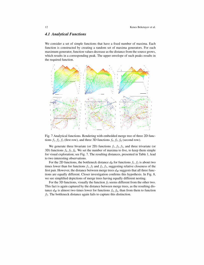
Fig. 7 Analytical functions. Rendering with embedded merge tree of three 2D func-tions f1, f2, f3 (first row), and three 3D functions f4, f5, f6 (second row).

We generate three bivariate (or 2D) functions f1, f2, f3, and three trivariate (or3D) functions f4, f5, f6. We set the number of maxima to five, to keep them simplefor visual exploration; see Fig. 7. The resulting distances, presented in Table 1, leadto two interesting observations.

For the 2D functions, the bottleneck distance dB for functions f1, f2 is about twotimes lower than for functions f1, f3 and f2, f3, suggesting relative closeness of thefirst pair. However, the distance between merge trees dM suggests that all three func-tions are equally different. Closer investigation confirms this hypothesis. In Fig. 8,we see simplified depictions of merge trees having equally different nesting.

For the 3D functions, visually the function f5 seems different from the other two.This fact is again captured by the distance between merge trees, as the resulting dis-tance dM is almost two times lower for functions f4, f6, than from them to functionf5. The bottleneck distance again fails to capture this distinction.

Measuring the Distance between Merge Trees 13Table 1 Resulting distances from Fig. 7.

Metric f 2D1 f 2D

2 f 2D3 f 3D

4 f 3D5 f 3D

6

dB 4.525 8.647 7 3.011 2.598 4.031dM 8.398 8.664 7 5.031 2.604 4.833L∞ 67.561 43.015 65.956 29.586 20.495 22.632

Fig. 8 Simplified view ofnesting of merge trees forfunctions f1, f2, f3. Unmatch-able red edges cause thenon-zero distance. Tf1 Tf2 Tf3

4.2 Tuning a Ray Tracing Algorithm

We consider the problem of tuning a ray tracing algorithm on a multicore shared-memory system from the study by Bethel and Howison [1]. The authors exploredvarious tuning parameters and their effect on the performance of the algorithm,with a focus on three parameters: the work block width {1,2, . . . ,512} and height{1,2, . . . ,512}, and the concurrency level {1,2,4,8}.

We generated two data sets with the same parameter space, but slightly differentalgorithm, based on the selection of a ray sampling method, which is either basedon nearest neighbor or trilinear approximation. For each option, the performance ofthe algorithm (in terms of running time) was recorded.

In this example, one is interested in studying optimal run configurations thatcorrespond to low run times of the algorithm. Fig. 9 shows two data sets usingisosurfaces, such that isovalues are the same for both data sets. The similarity ofdata sets, implying that the selection of the chosen ray sampling method does notsignificantly influence the performance of the algorithm. This fact is confirmed bythe resulting distance. The measured distances allow us to capture the similarity,regardless of shifted optimal configurations (minima) and the noise.

Fig. 9 Performance data. dB = 0.027,dM = 0.027,L∞ = 0.13. The difference is smallrelative to the value range of functions (about 2.7%), implying little influence of theray sampling option on the overall performance of the algorithm.

5 Conclusions

We presented a novel distance between merge trees, including the definition and thealgorithm. We demonstrated the use of the proposed distance for several data sets.

We plan to perform a theoretical investigation of the proposed distance, includingthe concerns about its stability. We also plan to explore the use of the proposeddistance for error analysis in the context of approximated scalar functions.


Acknowledgements The authors thank Aidos Abzhanov. This work was supported by the Direc-tor, Office of Advanced Scientific Computing Research, Office of Science, of the U.S. DOE underContract No. DE-AC02-05CH11231 (Berkeley Lab), and the Program 055 of the Ministry of Edu.and Sci. of the Rep. of Kazakhstan under the contract with the CER, Nazarbayev University.

References

1. Bethel, E.W., Howison, M.: Multi-core and many-core shared-memory parallel raycasting vol-ume rendering optimization and tuning. Int. Journal of High Perf. Comput. Appl. (2012)

2. Biasotti, S., De Floriani, L., Falcidieno, B., Frosini, P., Giorgi, D., Landi, C., Papaleo, L.,Spagnuolo, M.: Describing shapes by geometrical-topological properties of real functions.ACM Computing Surveys 40, 12:1–12:87 (2008)

3. Biasotti, S., Marini, M., Spagnuolo, M., Falcidieno, B.: Sub-part correspondence by structuraldescriptors of 3D shapes. Computer Aided Design 38(9), 1002–1019 (2006)

4. Bille, P.: A survey on tree edit distance and related problems. Journal of Theor. Comp. Sci.337, 217–239 (2005)

5. Boyell, R.L., Ruston, H.: Hybrid techniques for real-time radar simulation. In: Proc. of theFall Joint Comput. Conf., pp. 445–458. IEEE (1963)

6. Bunke, H., Riesen, K.: Graph Edit Distance: Optimal and Suboptimal Algorithms with Appli-cations, pp. 113–143. Wiley-VCH Verlag GmbH & Co. KGaA (2009)

7. Carr, H., Snoeyink, J., Axen, U.: Computing contour trees in all dimensions. Comp. Geom. –Theory and Appl. 24(2), 75–94 (2003)

8. Cohen-Steiner, D., Edelsbrunner, H., Harer, J.: Stability of persistence diagrams. In: Proc. of21st Annual Symp. on Comp. Geom., pp. 263–271. ACM (2005)

9. Edelsbrunner, H., Harer, J., Natarajan, V., Pascucci, V.: Morse-Smale complexes for piecewiselinear 3-manifolds. In: Proc. of the 19th Symp. on Comp. Geom., pp. 361–370 (2003)

10. Edelsbrunner, H., Harer, J., Zomorodian, A.: Hierarchical Morse-Smale complexes for piece-wise linear 2-manifold. Disc. & Comp. Geom. 30, 87–107 (2003)

11. Flamm, C., Hofacker, I.L., Stadler, P., Wolfinger, M.: Barrier trees of degenerate landscapes.Physical Chemistry 216, 155–173 (2002)

12. Gerber, S., Bremer, P.T., Pascucci, V., Whitaker, R.: Visual exploration of high dimensionalscalar functions. IEEE Trans. Vis. Comput. Graph. 16(6) (2010)

13. Heine, C., Scheuermann, G., Flamm, C., Hofacker, I.L., Stadler, P.F.: Visualization of barriertree sequences. IEEE Trans. Vis. Comp. Graph. 12(5), 781–788 (2006)

14. Hilaga, M., Shinagawa, Y., Kohmura, T., Kunii, T.L.: Topology matching for fully automaticsimilarity estimation of 3d shapes. In: SIGGRAPH’01, pp. 203–212. ACM (2001)

15. Jiang, T., Lawler, E., Wang, L.: Aligning sequences via an evolutionary tree: complexity andapproximation. In: Symp. on Theory of Computing, pp. 760–769 (1994)

16. Milnor, J.W.: Morse Theory. Princeton University Press, Princeton, New Jersey (1963)17. Munkres, J.R.: Elements of Algebraic Topology. Addison-Wesley, Redwood City, CA (1984)18. Oesterling, P., Heine, C., Janicke, H., Scheuermann, G., Heyer, G.: Visualization of high-

dimensional point clouds using their density distribution’s topology. IEEE Trans. Vis. Comput.Graph. 17, 1547–1559 (2011)

19. Pascucci, V., Cole-McLaughlin, K., Scorzelli, G.: Multi-resolution computation and presenta-tion of contour trees. Tech. Rep. UCRL-PROC-208680, LLNL (2005)

20. Pascucci, V., Scorzelli, G., Bremer, P.T., Mascarenhas, A.: Robust on-line computation ofReeb graphs: Simplicity and speed. ACM Trans. on Graph. 26(3), 58.1–58.9 (2007)

21. Reeb, G.: Sur les points singuliers d’une forme de pfaff complement intergrable ou d’unefonction numerique. Comptes Rendus Acad. Science Paris 222, 847–849 (1946)

22. Thomas, D.M., Natarajan, V.: Symmetry in scalar field topology. IEEE Trans. Vis. Comput.Graph. 17(12), 2035–2044 (2011)

23. Weber, G.H., Bremer, P.T., Pascucci, V.: Topological landscapes: A terrain metaphor for sci-entific data. IEEE Trans. Vis. Comput. Graph. 13(6), 1416–1423 (2007)

measuring the distance between mer ge t...

Documents