Measuring the Bias of Technological Change∗

Ulrich Doraszelski†

University of Pennsylvania

Jordi Jaumandreu‡

Boston University

This draft: February 5, 2017

First draft: December 13, 2008

Abstract

Technological change can increase the productivity of the various factors of produc-

tion in equal terms, or it can be biased towards a specific factor. We directly assess

the bias of technological change by measuring, at the level of the individual firm, how

much of it is labor augmenting and how much is factor neutral. To do so, we develop a

framework for estimating production functions when productivity is multi-dimensional.

Using panel data from Spain, we find that technological change is biased, with both its

labor-augmenting and its factor-neutral components causing output to grow by about

1.5% per year.

∗We thank the Editor Ali Hortacsu, two anonymous referees, Pol Antras, Paul David, Matthias Doepke,

Michaela Draganska, Jose Carlos Farinas, Ivan Fernandez-Val, Paul Grieco, Chad Jones, Dale Jorgenson,

Larry Katz, Pete Klenow, Jacques Mairesse, Ariel Pakes, Amil Petrin, Zhongjun Qu, Devesh Raval, Juan

Sanchis, Matthias Schundeln, Johannes Van Biesebroeck, John Van Reenen, and Hongsong Zhang for helpful

comments and discussions and Tianyi Chen, Sterling Horne, Mosha Huang, Thomas O’Malley, and Dan Sacks

for research assistance. We gratefully acknowledge financial support from the National Science Foundation

under Grants No. 0924380 and 0924282; Jaumandreu further acknowledges partial funding from Fundacion

Rafael del Pino.†Wharton School, University of Pennsylvania, Steinberg Hall-Dietrich Hall, 3620 Locust Walk, Philadel-

phia, PA 19104, USA. E-mail: doraszelski@wharton.upenn.edu.‡Department of Economics, Boston University, 270 Bay State Road, Boston, MA 02215, USA. E-mail:

jordij@bu.edu.

1 Introduction

When technological change occurs, it can increase the productivity of capital, labor, and

the other factors of production in equal terms, or it can be biased towards a specific factor.

Whether technological change favors some factors of production over others is central to

economics. Yet, the empirical evidence is relatively sparse.

The literature on economic growth rests on the assumption that technological change

increases the productivity of labor vis-a-vis the other factors of production. It is well known

that for a neoclassical growth model to exhibit steady-state growth, either the production

function must be Cobb-Douglas or technological change must be labor augmenting (Uzawa

1961), and many endogenous growth models point to human capital accumulation as a

source of productivity increases (Lucas 1988, Romer 1990). A number of recent papers

provide microfoundations for the literature on economic growth by theoretically establishing

that profit-maximizing incentives can ensure that technological change is, at least in the

long run, purely labor augmenting (Acemoglu 2003, Jones 2005). Whether this is indeed

the case is, however, an empirical question that remains to be answered.

One reason for the scarcity of empirical assessments of the bias of technological change

may be a lack of suitable data. Following early work by Brown & de Cani (1963) and

David & van de Klundert (1965), economists have estimated aggregate production or cost

functions that proxy for labor-augmenting technological change with a time trend (Lucas

1969, Kalt 1978, Antras 2004, Klump, McAdam & Willman 2007, Binswanger 1974, Cain

& Paterson 1986, Jin & Jorgenson 2010).1 While this line of research has produced some

evidence of labor-augmenting technological change, the staggering amount of heterogeneity

across firms in combination with simultaneously occurring entry and exit (Dunne, Roberts

& Samuelson 1988, Davis & Haltiwanger 1992) may make it difficult to interpret a time

trend as a meaningful average economy- or sector-wide measure of technological change.

Furthermore, this line of research pays scant attention to the fundamental endogeneity

problem in production function estimation. This problem arises because a firm’s decisions

depend on its productivity, and productivity is not observed by the econometrician, and

may severely bias the estimates (Marschak & Andrews 1944).

While traditionally using more disaggregated data, the productivity and industrial or-

ganization literatures assume that technological change is factor neutral. Hicks-neutral

technological change underlies, either explicitly or implicitly, most of the standard tech-

niques for measuring productivity, ranging from the classic growth decompositions of Solow

(1957) and Hall (1988) to the recent structural estimators for production functions (Olley

& Pakes 1996, Levinsohn & Petrin 2003, Ackerberg, Caves & Frazer 2015, Doraszelski &

Jaumandreu 2013, Gandhi, Navarro & Rivers 2013).

1A much larger literature has estimated the elasticity of substitution using either aggregated or disag-gregated data whilst maintaining the assumption of factor-neutral technological change, see Hammermesh(1993) for a survey.

2

In this paper, we extend the productivity and industrial organization literatures and de-

velop a framework for estimating production functions when productivity is multi-dimensional

and has a labor-augmenting and a Hicks-neutral component. We use firm-level panel data

that is now widely available to directly assess the bias of technological change by measuring,

at the level of the individual firm, how much of technological change is labor augmenting

and how much of it is Hicks neutral.

To tackle the endogeneity problem in production function estimation, we build on the

insight of Olley & Pakes (1996) that if the decisions that a firm makes can be used to infer its

productivity, then productivity can be controlled for in the estimation. We infer the firm’s

multi-dimensional productivity from its input usage, in particular its labor and materials

decisions. The key to identifying the bias of technological change is that Hicks-neutral

technological change scales input usage but, in contrast to labor-augmenting technological

change, does not change the mix of inputs that a firm uses. A change in the input mix

therefore contains information about the bias of technological change, provided we control

for the relative prices of the various inputs and other factors that may change the input

mix.

We apply our framework to examine the speed and direction of technological change

in the Spanish manufacturing sector in the 1990s and early 2000s. Spain is an attractive

setting for two reasons. First, Spain became fully integrated into the European Union

between the end of the 1980s and the beginning of the 1990s. Any trends in technological

change that our analysis uncovers for Spain may thus be viewed as broadly representative

for other continental European economies. Second, Spain inherited an industrial structure

with few high-tech industries and mostly small and medium-sized firms. R&D is widely

seen as lacking. Yet, Spain grew rapidly during the 1990s, and R&D became increasingly

important (European Commission 2001). The accompanying changes in industrial structure

are a useful source of variation for analyzing the role of R&D in stimulating different types

of technological change.

The particular data set we use has several advantages. The broad coverage allows us

to assess the bias of technological change in industries that differ greatly in terms of firms’

R&D activities. The data set also has an unusually long time dimension, enabling us to

disentangle trends in technological change from short-term fluctuations. Finally, the data

set has firm-level prices that we exploit heavily in the estimation.2

The Spanish manufacturing sector also poses several challenges for identifying the bias of

technological change from a change in the mix of inputs that a firm uses. First, outsourcing

directly changes the input mix as the firm procures customized parts and pieces from its

2There are other firm-level data sets such as the Colombian Annual Manufacturers Survey (Eslava,Haltiwanger, Kugler & Kugler 2004), the Prowess data collected by the Centre for Monitoring the IndianEconomy (De Loecker, Goldberg, Khandelwal & Pavcnik 2016), and the Longitudinal Business Database atthe U.S. Census Bureau that contain separate information on prices and quantities, at least for a subset ofindustries (Roberts & Supina 1996, Foster, Haltiwanger & Syverson 2008, Foster, Haltiwanger & Syverson2016).

3

suppliers rather than makes them in house from scratch. Second, the Spanish labor market

manifestly distinguishes between permanent and temporary labor. We further contribute

to the literature following Olley & Pakes (1996) by accounting for outsourcing and the dual

nature of the labor market.

Our estimates provide clear evidence that technological change is biased. Ceteris paribus

labor-augmenting technological change causes output to grow, on average, in the vicinity

of 1.5% per year. While there is a shift from unskilled to skilled workers in our data, this

skill upgrading explains some but not all of the growth of labor-augmenting productivity.

In many industries, labor-augmenting productivity grows because workers with a given set

of skills become more productive over time.

At the same time, our estimates show that Hicks-neutral technological change plays an

equally important role. In addition to labor-augmenting technological change, Hicks-neutral

technological change causes output to grow, on average, in the vicinity of 1.5% per year.

Behind these averages lies a substantial amount of heterogeneity across industries and

firms. Our estimates point to substantial and persistent differences in labor-augmenting and

Hicks-neutral productivity across firms, in line with the “stylized facts” about productivity

in Bartelsman & Doms (2000) and Syverson (2011). Beyond these facts, we show that, at the

level of the individual firm, the levels of labor-augmenting and Hicks-neutral productivity

are positively correlated, as are their rates of growth.

Our estimates further indicate that firms’ R&D activities play a key role in determining

the differences in the components of productivity across firms and their evolution over

time. Interestingly, labor-augmenting productivity is slightly more closely tied to firms’

R&D activities than is Hicks-neutral productivity. Through the lens of the literature on

induced innovation and directed technical change (Hicks 1932, Acemoglu 2002), this may

be viewed as supporting the argument that firms direct their R&D activities to conserve on

labor.

Biased technological change has consequence far beyond the growth of output. To

illustrate, we use our estimates to show that biased technological change is the primary

driver of the decline of the aggregate share of labor in the Spanish manufacturing sector

over our sample period. Similar declines have been observed in many advanced economies

in past decades and have attracted considerable attention in the macroeconomics literature

(Blanchard 1997, Bentolila & Saint-Paul 2004, McAdam & Willman 2013, Karabarbounis

& Neiman 2014, Oberfield & Raval 2014).

The starting point of this paper are the recent structural estimators for production func-

tions. We differ from much of the previous literature by exploiting the parameter restric-

tions between the production and input demand functions, as in Doraszelski & Jaumandreu

(2013). This allows us to parametrically invert from observed input usage to unobserved

productivity and eases the demands on the data compared to the nonparametric inversion

in Olley & Pakes (1996), Levinsohn & Petrin (2003), and Ackerberg et al. (2015), especially

4

if the input demand functions are high-dimensional.3

Our paper is related to Van Biesebroeck (2003). Using plant-level panel data for the

U.S. automobile industry, he estimates a plant’s Hicks-neutral productivity as a fixed effect

and parametrically inverts from the plant’s input usage to its capital-biased (also called

labor-saving) productivity. Our approach is more general in that we allow all components

of productivity to evolve over time and in response to firms’ R&D activities.

Our paper is further related to Grieco, Li & Zhang (2016) and subsequent work in

progress by Zhang (2015). Because their data contains the materials bill rather than its

split into price and quantity, Grieco et al. (2016) build on Doraszelski & Jaumandreu (2013)

and parametrically invert from a firm’s input usage to its Hicks-neutral productivity and

the price of materials that the firm faces.

Finally, our paper touches—although more tangentially—on the literature on skill bias

that studies the differential impact of technological change, especially in the form of com-

puterization, on the various types of labor (see Card & DiNardo (2002) and Violante (2008)

and the references therein). While we focus on labor versus the other factors of produc-

tion, the techniques we develop may be adapted to investigate the skill bias of technological

change, although our particular data set is not ideal for this purpose.

The remainder of this paper is organized as follows: Section 2 explains how we identify

the bias of technological change and previews our empirical strategy. Section 3 describes

the data and some patterns in the data that inform the subsequent analysis. Section 4 sets

out a dynamic model of the firm. Section 5 develops an estimator for production functions

when productivity is multi-dimensional. Sections 6–9 present our main results on labor-

augmenting and Hicks-neutral technological change. Section 10 explores whether capital-

augmenting technological change plays a role in our data in addition to labor-augmenting

and Hicks-neutral technological change. Section 11 concludes. An Online Appendix contains

additional results and technical details.

Throughout the paper, we adopt the convention that uppercase letters denote levels and

lowercase letters denote logs. Unless noted otherwise, we refer to output and the various

factors of production in terms of quantity and not in terms of value. In particular, we refer

to the value of labor as the wage bill and to the value of materials as the materials bill.

2 Labor-augmenting and Hicks-neutral productivity

We first show how to separately recover a firm’s labor-augmenting and Hicks-neutral pro-

ductivity from its labor and materials decisions. Then we show that the constant elasticity

of substitution (CES) production function that we use in our application approximates, to

a first order, the relationship between the input mix and labor-augmenting productivity

that arises in a wider class of production functions. To facilitate the exposition, we proceed

3See Doraszelski & Jaumandreu (2013) for details on the pros and cons of the parametric inversion.

5

in a highly simplified setting. Our application extends the setting to accommodate the

institutional realities of the Spanish manufacturing sector.

Consider a firm with the production function

Yjt = F (Kjt, exp(ωLjt)Ljt,Mjt) exp(ωHjt) exp(ejt), (1)

where Yjt is the output of firm j in period t, Kjt is capital, Ljt is labor, and Mjt is

materials. The labor-augmenting productivity of firm j in period t is ωLjt and its Hicks-

neutral productivity is ωHjt. Finally, ejt is a random shock.

To relate the input ratioMjt

Ljtto labor-augmenting productivity ωLjt, we assume that

(exp(ωLjt)Ljt,Mjt) is separable from Kjt in that the function F (·) in equation (1) is com-

posed of the functions G(·) and H(·) as

F (Kjt, exp(ωLjt)Ljt,Mjt) = G(Kjt, H(exp(ωLjt)Ljt,Mjt)), (2)

whereH(exp(ωLjt)Ljt,Mjt) is homogeneous of arbitrary degree.4 Without loss of generality,

we set the degree of homogeneity to one. Throughout we maintain that all functions are

differentiable as needed. As in Levinsohn & Petrin (2003), we finally assume that labor

and materials are static (or “variable”) inputs that are chosen each period to maximize

short-run profits and that the firm is a price-taker in input markets, where it faces Wjt and

PMjt as prices of labor and materials, respectively.

The input ratioMjt

Ljtis therefore the solution to the ratio of the first-order conditions for

labor and materials

∂H(exp(ωLjt)Ljt,Mjt)∂Ljt

exp(ωLjt)

∂H(exp(ωLjt)Ljt,Mjt)∂Mjt

=

∂H(exp(ωLjt−(mjt−ljt)),1)∂Ljt

exp(ωLjt)

∂H(exp(ωLjt−(mjt−ljt)),1)∂Mjt

=Wjt

PMjt, (3)

where the first equality uses that H(exp(ωLjt)Ljt,Mjt) is homogeneous of degree one and,

recall, uppercase letters denote levels and lowercase letters denote logs.

Equation (3) implies that the input ratioMjt

Ljtdepends on the price ratio

PMjt

Wjtand labor-

augmenting productivity ωLjt. Importantly, the input ratioMjt

Ljtdoes not depend on Hicks-

neutral productivity ωHjt. This formalizes that the mix of inputs that a firm uses is related

to—and therefore contains information about—its labor-augmenting productivity but is

unrelated to its Hicks-neutral productivity. Intuitively, the labor and materials decisions

hinge on the marginal products of labor and materials. Because the marginal products are

proportional to Hicks-neutral productivity, materials per unit of labor as determined by the

ratio of the first-order conditions in equation (3) is unrelated to Hicks-neutral productivity.

4Equation (2) immediately implies that F (Kjt, exp(ωLjt)Ljt,Mjt) is weakly separable in the partition(Kjt, (exp(ωLjt)Ljt,Mjt)) (Chambers 1988, equation (1.26)). It is equivalent to F (Kjt, exp(ωLjt)Ljt,Mjt)being weakly separable under some additional monotonicity and quasi-concavity assumptions (Goldman &Uzawa 1964).

6

In this sense, separating labor-augmenting from Hicks-neutral productivity does not rely

on functional form beyond the separability assumption in equation (2).5

The following proposition further characterizes the log of the input ratio mjt − ljt:

Proposition 1 The input ratio mjt − ljt has the first-order Taylor series

γ0L − σ

(exp(ω0

Ljt − (m0jt − l0jt))

)(pMjt − wjt) +

(1− σ

(exp(ω0

Ljt − (m0jt − l0jt))

))ωLjt (4)

around a point (m0jt − l0jt, p0

Mjt − w0jt, ω

0Ljt) satisfying equation (3), where γ0

L is a constant

and σ(

exp(ω0Ljt − (m0

jt − l0jt)))

is the elasticity of substitution between materials and labor

in the production function in equation (1).

The proof can be found in Appendix A.

Our application uses a CES production function

Yjt =

[βKK

− 1−σσ

jt + (exp(ωLjt)Ljt)− 1−σ

σ + βMM− 1−σ

σjt

]− νσ1−σ

exp(ωHjt) exp(ejt),

where ν and σ are the elasticity of scale and substitution, respectively, and βK and βM

are the so-called distributional parameters.6 Depending on the elasticity of substitution,

the CES production function encompasses the special cases of a Leontieff (σ → 0), Cobb-

Douglas (σ = 1), and linear (σ →∞) production function.

The ratio of the first-order conditions in equation (3) implies

mjt − ljt = σ lnβM − σ(pMjt − wjt) + (1− σ)ωLjt. (5)

Comparing equations (4) and (5) shows that the CES production function approximates,

to a first order, the input ratio mjt − ljt arising from an arbitrary production function

satisfying equation (2). This gives a sense of robustness to the CES production function.7

Our empirical strategy uses equation (5) to recover a firm’s labor-augmenting produc-

tivity from its input mix. In doing so, we must control for other factors besides the relative

prices of the various inputs that may change the input mix, in particular outsourcing and

the dual nature of the Spanish labor market. With labor-augmenting productivity in hand,

5One can forgo the separability assumption by relying more on functional form. Our empirical strategygeneralizes to, for example, a translog production function that does not satisfy equation (2).

6We implicitly set the constant of proportionality β0 to one because it cannot be separated from anadditive constant in Hicks-neutral productivity ωHjt. We estimate them jointly and carefully ensure thatthe reported results depend only on their sum. We similarly normalize the distributional parameter βL.Technological change can therefore equivalently be thought of as letting these parameters of the productionfunction vary by firm and time. The nascent literature on heterogeneous production functions (Balat,Brambilla & Sasaki 2015, Fox, Hadad, Hoderlein, Petrin & Sherman 2016, Kasahara, Schrimpf & Suzuki2015) explores to what extent it is possible to let all parameters of the production function vary by firm andtime.

7It also suggests that our “nonparametric” estimates of labor-augmenting technological change can befed into a growth decomposition along the lines of Solow (1957) and Hall (1988) to obtain a “nonparametric”estimate of Hicks-neutral technological change. We leave this to future research.

7

we use the first-order condition for labor to recover Hicks-neutral productivity. The remain-

der of our empirical strategy follows along the lines of Olley & Pakes (1996), Levinsohn &

Petrin (2003), Ackerberg et al. (2015), and Doraszelski & Jaumandreu (2013) by combining

the inferred productivities with their laws of motion to set up estimation equations.

Equation (5) has a long tradition in the literature, although it is used in a very different

way from ours. With skilled and unskilled workers in place of materials and labor, equation

(5) is at the heart of the literature on skill bias (Card & DiNardo 2002, Violante 2008). With

capital in place of materials, equation (5) serves to estimate the elasticity of substitution σ

in an aggregate value-added production function (see Antras 2004). More recently, Raval

(2013) uses a variant of equation (5) obtained from a value-added production function with

capital- and labor-augmenting productivity to estimate σ from firm-level panel data.

Equation (5) is typically estimated by OLS. The problem is that labor-augmenting

productivity, which is not observed by the econometrician, is correlated over time and also

with the wage. We intuitively expect the wage to be higher when labor is more productive,

even if it adjusts slowly with some lag. This positive correlation induces an upward bias in

the estimate of the elasticity of substitution. This is a variant of the endogeneity problem in

production function estimation. Because we use equation (5) to recover labor-augmenting

productivity rather than directly estimate it, we are able tackle the endogeneity problem

with a combination of assumptions on the timing of decisions and the evolution of the

components of productivity.

3 Data

Our data comes from the Encuesta Sobre Estrategias Empresariales (ESEE) survey, a firm-

level survey of the Spanish manufacturing sector sponsored by the Ministry of Industry,

and spans 1990 to 2006. At the beginning of the survey, 5% of firms with up to 200 workers

were sampled randomly by industry and size strata. All firms with more than 200 workers

were asked to participate in the survey, and 70% of them complied. Some firms vanish from

the sample due to either exit (shutdown by death or abandonment of activity) or attrition.

These reasons can be distinguished in the data and attrition remained within acceptable

limits. To preserve representativeness, newly created firms were added to the sample every

year. We provide details on industry and variable definitions in Appendix B.

Our sample covers a total of 2375 firms in ten industries when restricted to firms with at

least three years of data. Columns (1) and (2) of Table 1 show the number of observations

and firms by industry. Sample sizes are moderate. Newly created firms are a large fraction

of the total number of firms, ranging from 26% to 50% in the different industries. There

is a much smaller fraction of exiting firms, ranging from 6% to 15% and above in a few

industries.

The 1990s and early 2000s were a period of rapid output growth, coupled with stagnant

8

or, at best, slightly increasing employment and intense investment in physical capital, see

columns (3)–(6) of Table 1. Consistent with this rapid growth, firms on average report that

their markets are slightly more often expanding rather than contracting; hence, demand

tends to shift out over time.

An attractive feature of our data is that it contains firm-specific, Paasche-type price

indices for output and materials. We note that the variation in these price indices is partly

due to changes over time in the bundles of goods that make up output and, respectively,

materials (see Bernard, Redding & Schott (2010) and Goldberg, Khandelwal, Pavcnik &

Topalova (2010) for evidence on product turnover), and that these changes may be related to

a firm’s productivity. The growth of prices, averaged from the growth of prices as reported

individually by each firm, is moderate. The growth of the price of output in column (7)

ranges from 0.8% to 2.1%. The growth of the wage ranges from 4.3% to 5.4% and the

growth of the price of materials ranges from 2.8% to 4.1%.

Biased technological change. The evolution of the relative quantities and prices of

the various factors of production already hints at an important role for labor-augmenting

technological change. As columns (8) and (9) of Table 1 show, with the exception of

industries 7, 8, and 9, the input ratioMjt

Ljtincreases much more than the price ratio

PMjt

Wjt

decreases. One possible explanation is that the elasticity of substitution between materials

and labor exceeds 1. To see this, recall that the elasticity of substitution (Chambers 1988,

equation (1.12)) is

d ln(Mjt

Ljt

)d ln (|MRTSMLjt|)

= −d ln

(Mjt

Ljt

)d ln

(PMjt

Wjt

) ,where |MRTSMLjt| is the absolute value of the marginal rate of technological substitution

between materials and labor, and the equality follows to the extent that it equals the price

ratioPMjt

Wjt. However, because the estimates of the elasticity of substitution in the previous

literature lie somewhere between 0 and 1 (see Chirinko (2008) and the references therein

for the elasticity of substitution between capital and labor and Bruno (1984), Rotemberg &

Woodford (1996), and Oberfield & Raval (2014) for the elasticity of substitution between

materials and an aggregate of capital and labor), this explanation is implausible. Labor-

augmenting technological change offers an alternative explanation. As it makes labor more

productive, equation (4) implies that it directly increases materials per unit of labor. Thus,

labor-augmenting technological change may go a long way in rationalizing why the change

in the input ratioMjt

Ljtexceeds the change in the price ratio

PMjt

Wjt.

In contrast, columns (10) and (11) of Table 1 provide no evidence for capital-augmenting

technological change. The investment boom in Spain in the 1990s and early 2000s was fueled

by improved access to European and international capital markets. With the exception of

industries 5, 6, and 8, the concomitant decrease in the input ratioMjt

Kjtis much smaller than

9

the increase in the price ratioPMjt

PKjt, where PKjt is the price of capital as however roughly

measured by the user cost in our data. This pattern is consistent with an elasticity of

substitution between materials and capital between 0 and 1. Indeed, capital-augmenting

technological change can only directly contribute to the decline in materials per unit of

capital in the unlikely scenario that it makes capital less productive.

Based on these patterns in the data we focus on labor-augmenting technological change

in the subsequent analysis. We return to capital-augmenting technological change in Section

10. In the remainder of this section we point out other features of the data that figure

prominently in our analysis.

Temporary labor. We distinguish between permanent and temporary labor and treat

temporary labor as a static input that is chosen each period to maximize short-run profits.

This is appropriate because Spain greatly enhanced the possibilities for hiring and firing

temporary workers during the 1980s, and by the beginning of the 1990s had one the highest

shares of temporary workers in Europe (Dolado, Garcia-Serrano & Jimeno 2002). Tem-

porary workers are employed for fixed terms with no or very small severance pay. In our

sample, between 72% and 84% of firms use temporary labor and, among the firms that do,

its share of the labor force ranges from 16% in industry 10 to 32% in industry 9, see columns

(1) and (2) of Table 2.

Rapid expansions and contractions of temporary labor are common: The difference

between the maximum and the minimum share of temporary labor within a firm ranges

on average from 20% to 33% across industries (column (3)). In addition to distinguishing

temporary from permanent labor, we measure labor as hours worked (see Appendix B). At

this margin, firms enjoy a high degree of flexibility: Within a firm, the difference between

the maximum and the minimum hours worked ranges on average from 43% to 56% across

industries, and the difference between the maximum and the minimum hours per worker

ranges on average from 4% to 13% (columns (4) and (5)).

Outsourcing. Outsourcing may directly contribute to the shift from labor to materials

that column (8) of Table 1 documents as firms procure customized parts and pieces from

their suppliers rather than make them in house from scratch. As can be seen in columns

(6) and (7) of Table 2, between 21% and 57% of firms in our sample engage in outsourcing.

Among the firms that do, the share of outsourcing in the materials bill ranges from 14%

in industry 7 to 29% in industry 4. While the share of outsourcing remains stable over

our sample period, the standard deviation in column (7) indicates a substantial amount of

heterogeneity across the firms within an industry, similar to the share of temporary labor

in column (2).

Firms’ R&D activities. Columns (8)–(10) of Table 2 show that the ten industries differ

markedly in terms of firms’ R&D activities and that there is again substantial heterogeneity

10

across the firms within an industry. Industries 3, 4, 5, and 6 exhibit high innovative activity.

More than two-thirds of firms perform R&D during at least one year in the sample period,

with at least 36% of stable performers engaging in R&D in all years (column (8)) and at

least 28% of occasional performers engaging in R&D in some but not all years (column

(9)). The R&D intensity among performers ranges on average from 2.2% to 2.9% (column

(10)). Industries 1, 2, 7, and 8 are in an intermediate position. Less than half of firms

perform R&D, and there are fewer stable than occasional performers. The R&D intensity is

on average between 1.1% and 1.7% with a much lower value of 0.7% in industry 7. Finally,

industries 9 and 10 exhibit low innovative activity. About a third of firms perform R&D,

and the R&D intensity is on average between 1.0% and 1.5%.

4 A dynamic model of the firm

The purpose of our model is to enable us to infer a firm’s productivity from its input usage

and to clarify our assumptions on the timing of decisions that we rely on in estimation.

Production function. The firm has the CES production function

Yjt =

[βKK

− 1−σσ

jt +(exp(ωLjt)L

∗jt

)− 1−σσ + βM

(M∗jt

)− 1−σσ

]− νσ1−σ

exp(ωHjt) exp(ejt), (6)

where Yjt is the output of firm j in period t, Kjt is capital, ωLjt is labor-augmenting produc-

tivity, ωHjt is Hicks-neutral productivity, and ejt is a mean zero random shock that is uncor-

related over time and across firms. Extending the setting in Section 2, L∗jt = Λ(LPjt, LTjt) is

an aggregate of permanent labor LPjt and temporary labor LTjt and M∗jt = Γ(MIjt,MOjt)

is an aggregate of in-house materials MIjt and outsourced materials (customized parts and

pieces) MOjt. The aggregators Λ(LPjt, LTjt) and Γ(MIjt,MOjt) accommodate differences in

the productivities of permanent and temporary labor, respectively, in-house and outsourced

materials.

The production function in equation (6) is the most parsimonious we can use to separate

labor-augmenting from Hicks-neutral productivity. It encompasses three restrictions. First,

technological change does not affect the parameters ν and σ, as we are unaware of evidence

suggesting that the elasticity of scale or the elasticity of substitution varies over our sample

period. Second, the elasticity of substitution between capital, labor, and materials is the

same.8 We assess this restriction in Section 8. For now we note that previous estimates

of the elasticity of substitution between materials and an aggregate of capital and labor

(Bruno 1984, Rotemberg & Woodford 1996, Oberfield & Raval 2014) fall in the same range

as estimates of the elasticity of substitution between capital and labor (Chirinko 2008).

Third, the productivities of capital and materials are restricted to change at the same rate

8The elasticity of substitution between LPjt and LTjt, respectively, MIjt and MOjt depends on theaggregators Λ(LPjt, LTjt) and Γ(MIjt,MOjt) and may differ from σ.

11

and in lockstep with Hicks-neutral technological change.9 Treating capital and materials

the same is in line with the fact that both are, at least to a large extent, produced goods.

In contrast, labor is traditionally viewed as unique among the various factors of production,

and changes in its productivity are a tenet of the literature on economic growth. The

patterns in the data described in Section 3 further justify focusing on labor-augmenting

technological change.

Laws of motion: Productivity. The components of productivity are presumably corre-

lated with each other and over time and possibly also correlated across firms. As in Doraszel-

ski & Jaumandreu (2013), we endogenize productivity by incorporating R&D expenditures

into the model. We assume that the evolution of the components of productivity is governed

by controlled first-order, time-inhomogeneous Markov processes with transition probabili-

ties PLt+1(ωLjt+1|ωLjt, Rjt) and PHt+1(ωHjt+1|ωHjt, Rjt), where Rjt is R&D expenditures.

Despite their parsimony, these stochastic processes accommodate correlation between the

components of productivity.10 Moreover, because they are time-inhomogeneous, they ac-

commodate secular trends in productivity.

The firm knows its current productivity when it makes its decisions for period t and

anticipates the effect of R&D on its future productivity. The Markovian assumption implies

ωLjt+1 = Et [ωLjt+1|ωLjt, Rjt] + ξLjt+1 = gLt(ωLjt, Rjt) + ξLjt+1, (7)

ωHjt+1 = Et [ωHjt+1|ωHjt, Rjt] + ξHjt+1 = gHt(ωHjt, Rjt) + ξHjt+1. (8)

That is, actual labor-augmenting productivity ωLjt+1 in period t + 1 decomposes into ex-

pected labor-augmenting productivity gLt(ωLjt, Rjt) and a random shock ξLjt+1. This pro-

ductivity innovation is by construction mean independent (although not necessarily fully

independent) of ωLjt and Rjt. It captures the uncertainties that are naturally linked to pro-

ductivity as well as those that are inherent in the R&D process such as chance of discovery,

degree of applicability, and success in implementation. Nonlinearities in the link between

R&D and productivity are captured by the conditional expectation function gLt(·) that we

estimate nonparametrically along with the parameters of the production function. Actual

Hicks-neutral productivity ωHjt+1 decomposes similarly.

9A production function with capital-augmenting, labor-augmenting, and materials-augmenting produc-tivity that is homogeneous of arbitrary degree is equivalent to a production function with capital-augmenting,labor-augmenting, and Hicks-neutral productivity. Without loss of generality, we therefore subsume the com-mon component of capital-augmenting, labor-augmenting, and materials-augmenting technological changeinto Hicks-neutral productivity.

10Our empirical strategy generalizes to a joint Markov process Pt+1(ωLjt+1, ωHjt+1|ωLjt, ωHjt, rjt). WhileR&D is widely seen as a major source of productivity growth (Griliches 1998), our empirical strategy extendsto other sources such as technology adoption, learning-by-importing (Kasahara & Rodrigue 2008), andlearning-by-exporting (De Loecker 2013). Both extensions are demanding on the data, however, as theyincrease the dimensionality of the functions that must be nonparametrically estimated.

12

Laws of motion: Capital. Capital accumulates according to Kjt+1 = (1− δ)Kjt + Ijt,

where δ is the rate of depreciation. As in Olley & Pakes (1996), investment Ijt chosen in

period t becomes effective in period t+ 1. Choosing Ijt is therefore equivalent to choosing

Kjt+1.

Permanent labor. Permanent labor is subject to convex adjustment costs CLP (LPjt, LPjt−1)

that reflect the substantial cost of hiring and firing that the firm may incur (Hammermesh

1993). The choice of permanent labor thus may have dynamic implications. In contrast,

temporary labor is a static input.

Outsourcing. Outsourcing is, to a large extent, based on contractual relationships be-

tween the firm and its suppliers (Grossman & Helpman 2002, Grossman & Helpman 2005).

The ratio of outsourced to in-house materials QMjt =MOjt

MIjtis subject to (convex or not)

adjustment costs CQM (QMjt+1, QMjt) that stem from forming and dissolving these rela-

tionships. The firm must maintain QMjt but may scale MIjt and MOjt up or down at will;

in-house materials, in particular, is a static input.

Output and input markets. The firm has market power in the output market, e.g., be-

cause products are differentiated. Its inverse residual demand function P (Yjt, Djt) depends

on its output Yjt and the demand shifter Djt.11 The firm is a price-taker in input markets,

where it faces WPjt, WTjt, PIjt, and POjt as prices of permanent and temporary labor and

in-house and outsourced materials, respectively.

The demand shifter and the prices that the firm faces in input markets evolve according

to a Markov process that we do not further specify. As a consequence, the prices that the

firm faces in period t+1 may depend on its productivity in period t or on an average industry-

wide measure of productivity. Finally, the Markov process may be time-inhomogenous to

accommodate secular trends.

Bellman equation. The firm makes its decisions to maximize the expected net present

value of cash flows. In contrast to its labor-augmenting productivity ωLjt and its Hicks-

neutral productivity ωHjt, the firm does not know the random shock ejt when it makes

its decisions for period t. Letting Vt(·) denote the value function in period t, the Bellman

equation for the firm’s dynamic programming problem is

Vt(Ωjt) = maxKjt+1,LPjt,LTjt,QMjt+1,MIjt,Rjt

P(X− νσ

1−σjt exp(ωHjt), Djt

)X− νσ

1−σjt exp(ωHjt)µ

−CI(Kjt+1 − (1− δ)Kjt)−WPjtLPjt − CLP (LPjt, LPjt−1)−WTjtLTjt

− (PIjt + POjtQMjt)MIjt − CQM (QMjt+1, QMjt)− CR(Rjt)

11In general, the residual demand that the firm faces depends on its rivals’ prices. In taking the model tothe data, one may replace rivals’ prices by an aggregate price index or dummies, although this substantiallyincreases the dimensionality of the functions that must be nonparametrically estimated.

13

+1

1 + ρEt [Vt+1(Ωjt+1)|Ωjt, Rjt] , (9)

where

Xjt = βKK− 1−σ

σjt +

(exp(ωLjt)L

∗jt

)− 1−σσ + βM

(M∗jt

)− 1−σσ , µ = Et [exp(ejt)] ,

Ωjt = (Kjt, LPjt−1, QMjt, ωLjt, ωHjt,WPjt,WTjt, PIjt, POjt, Djt) is the vector of state vari-

ables, and ρ is the discount rate. CI(Ijt) and CR(Rjt) are the cost of investment and

R&D, respectively, and accommodate indivisibilities in investment and R&D projects. The

firm’s dynamic programming problem gives rise to policy functions that characterize its

investment and R&D decisions (and thus the values of Kjt+1 or, equivalently, Ijt and Rjt in

period t) as well as its input usage (LPjt, LTjt, QMjt+1, and MIjt). The labor and materials

decisions are central to our empirical strategy.

Inverse functions. From the first-order conditions for permanent labor, temporary labor,

and in-house materials we derive functions hL(·) and hH(·) that allow us to recover unob-

servable labor-augmenting and Hicks-neutral productivity from observables. Appendix C

contains detailed derivations.

We make several assumptions. First, our data has hours worked by permanent and

temporary workers Ljt = LPjt + LTjt and the (quantity) share of temporary labor STjt =LTjtLjt

. To map L∗jt in the production function in equation (6) to the data, we assume that the

aggregator Λ(LPjt, LTjt) is linearly homogenous. This implies L∗jt = LjtΛ(1 − STjt, STjt).Moreover, because our data combines the wages of permanent and temporary workers into

Wjt = WPjt(1− STjt) +WTjtSTjt, we assume thatWPjt

WTjt= λ0 is an (unknown) constant.12

Second, our data has the materials bill PMjtMjt = PIjtMIjt + POjtMOjt, the (value)

share of outsourced materials SOjt =POjtMOjt

PMjtMjt, and the price of materials PMjt. To connect

the model with the data, we assume PMjt = PIjt+POjtQMjt so that the price of materials is

the effective cost of an additional unit of in-house materials. This implies Mjt = MIjt. We

further assume thatPIjtPOjt

= γ0 is an (unknown) constant and that Γ(MIjt,MOjt) is linearly

homogenous. This implies M∗jt = MjtΓ(

1, γ0SOjt

1−SOjt

). We finally normalize Γ(MIjt, 0) =

MIjt.

Third, the first-order condition for permanent labor involves a gap ∆jt between the

wage of permanent workers WPjt and their shadow wage. We exploit the fact that we

have three first-order conditions to substitute out for ∆jt in the inverse functions hL(·) and

hH(·). As this presumes interior solutions for permanent and temporary labor, we exclude

observations with STjt = 0 and thus LTjt = 0 from the subsequent analysis.13

12In the Online Appendix, we use a wage regression to estimate wage premia of various types of labor.We show that the wage premia do not change much if at all over time in line with our assumption that theratio

WPjt

WLjtis constant.

13Compare columns (1) and (2) of Tables 1 and 3 with columns (1) and (2) of Table 4 for the exact number

14

Taken together, our assumptions allow us to recover (conveniently rescaled) labor-

augmenting productivity ωLjt = (1− σ)ωLjt and Hicks-neutral productivity ωHjt as

ωLjt = γL +mjt − ljt + σ(pMjt − wjt)− σλ2(STjt) + (1− σ)γ1(SOjt)

≡ hL(mjt − ljt, pMjt − wjt, STjt, SOjt), (10)

ωHjt = γH +1

σmjt + pMjt − pjt − ln

(1− 1

η(pjt, Djt)

)+

(1 +

νσ

1− σ

)xjt +

1− σσ

γ1(SOjt)

≡ hH(kjt,mjt, SMjt, pjt, pMjt, Djt, STjt, SOjt), (11)

where γL = −σ lnβM , γH = − ln (νβMµ), η(pjt, Djt) is the absolute value of the price

elasticity of the residual demand that the firm faces,

Xjt = βKK− 1−σ

σjt + βM (Mjt exp (γ1(SOjt)))

− 1−σσ

(1− SMjt

SMjtλ1(STjt) + 1

),

and SMjt =PMjtMjt

V Cjtis the share of materials in variable cost V Cjt = WjtLjt + PMjtMjt.

Without loss of generality, we set βK + βM = 1 in what follows.

We treat λ1(STjt), λ2(STjt), and γ1(SOjt) as (unknown) functions of the share of tempo-

rary labor STjt, respectively, the share of outsourced materials SOjt that must be estimated

nonparametrically along with the parameters of the production function. We thus think of

λ1(STjt), λ2(STjt), and γ1(SOjt) as “correction terms” on labor and, respectively, materials

that help account for the substantial heterogeneity across the firms within an industry. Be-

cause we estimate these terms nonparametrically, they can accommodate different theories

about the Spanish labor market and the role of outsourcing. For example, we develop an

alternative model of outsourcing in the Online Appendix that assumes that both in-house

and outsourced materials are static inputs that the firm may mix and match at will, thereby

dispensing with the costly-to-adjust ratio of outsourced to in-house materials.

5 Empirical strategy

We combine the inverse functions in equations (10) and (11) with the laws of motion for

labor-augmenting and Hicks-neutral productivity in equations (7) and (8) into estimation

equations for the parameters of the production function in equation (6).

Labor-augmenting productivity. Substituting the inverse function in equation (10)

into the law of motion in equation (7), we form our first estimation equation

mjt − ljt = −σ(pMjt − wjt) + σλ2(STjt)− (1− σ)γ1(SOjt)

of observations and firms we exclude.

15

+gLt−1(hL(mjt−1 − ljt−1, pMjt−1 − wjt−1, STjt−1, SOjt−1), Rjt−1) + ξLjt, (12)

where the (conveniently rescaled) conditional expectation function is

gLt−1(hL(·), Rjt−1) = (1− σ)gLt−1

(hL(·)1− σ

,Rjt−1

)

and ξLjt = (1− σ)ξLjt.14

We allow gLt−1(hL(·), Rjt−1) to differ between zero and positive R&D expenditures and

specify

gLt−1(hL(·), Rt−1) = gL0(t− 1) + 1(Rjt−1 = 0)gL1(hL(·)) + 1(Rjt−1 > 0)gL2(hL(·), rjt−1),

(13)

where 1(·) is the indicator function and the functions gL1(hL(·)) and gL2(hL(·), rjt−1)

are modeled as described in Appendix D. Because the Markov process governing labor-

augmenting productivity is time-inhomogeneous, we allow the conditional expectation func-

tion gLt−1(hL(·), Rjt−1) to shift over time by gL0(t − 1). In practice, we model this shift

with time dummies.

Compared to directly estimating equation (5) by OLS, equation (12) intuitively dimin-

ishes the endogeneity problem because breaking out the part of ωLjt that is observable

via the conditional expectation function gLt−1(·) leaves “less” in the error term. This also

facilitates instrumenting for any remaining correlation between the included variables and

the error term.

In our model, labor ljt, materials mjt, the wage wjt, and the share of temporary labor

STjt are correlated with the productivity innovation ξLjt (since ξLjt is part of ωLjt). Note

that wjt = ln (WPjt(1− STjt) +WTjtSTjt) may be correlated with ξLjt even though the

firm takes the wage of permanent workers WPjt and the wage of temporary workers WTjt

as given because STjt may depend on ωLjt and ωHjt through equations (21) and (22). We

therefore base estimation on the moment conditions

E[ALjt(zjt)ξLjt

]= 0, (14)

where ALjt(zjt) is a vector of functions of the exogenous variables zjt as described in Ap-

pendix D.

In considering instruments it is important to keep in mind that equation (12) models the

evolution of labor-augmenting productivity ωLjt. As a consequence, instruments have to

14Equation (12) is a semiparametric, partially linear, model with the additional restriction that the inverse

function hL(·) is of known form. Identification in the sense of the ability to separate the parametric andnonparametric parts of the model follows from standard arguments (Robinson 1988, Newey, Powell & Vella1999).

16

be uncorrelated with the productivity innovation ξLjt but not necessarily with productivity

itself. Because ξLjt is the innovation to productivity ωLjt in period t, it is not known to the

firm when it makes its decisions in period t−1. All past decisions are therefore uncorrelated

with ξLjt. In particular, having been decided in period t−1, ljt−1 and mjt−1 are uncorrelated

with ξLjt, although they are correlated with ωLjt as long as productivity is correlated over

time. Similarly, because STjt−1 and thus wjt−1 = ln (WPjt−1(1− STjt−1) +WTjt−1STjt−1)

are determined in period t− 1, they are uncorrelated with the productivity innovation ξLjt

in period t. We therefore use lagged labor ljt−1, lagged materials mjt−1, and the lagged

wage wjt−1 for instruments.

In contrast to the wage wjt, in our model the price of materials pMjt = ln (PIjt + POjtQMjt)

is uncorrelated with ξLjt because the ratio of outsourced to in-house materials QMjt is de-

termined in period t − 1. For the same reason, the share of outsourced materials SOjt =POjtQMjt

PIjt+POjtQMjtis uncorrelated with ξLjt. We nevertheless choose to err on the side of caution

and restrict ourselves to the lagged price of materials pMjt−1 and the lagged share of out-

sourcing SOjt−1 for instruments. Finally, time t and the demand shifter Djt are exogenous

by construction and we use them for instruments.

The reasoning that the timing of decisions and the Markovian assumption on the evo-

lution of productivity taken together imply that all past decisions are uncorrelated with

productivity innovations originates in Olley & Pakes (1996). The subsequent literature

uses it to justify lagged input quantities as instruments (see, e.g., Section 2.4.1 of Acker-

berg, Benkard, Berry & Pakes (2007)). In Doraszelski & Jaumandreu (2013), we extend

this reasoning to justify lagged output and input prices as instruments (pp. 1347–1348).

More recently, De Loecker et al. (2016) do the same to justify the lagged price of output as

instrument (p. 471).

A test for overidentifying restrictions in Section 6 cannot reject the validity of the

moment conditions in equation (14). More targeted tests and additional checks further

suggest that there is limited reason to doubt that wjt−1 and pMjt−1 are uncorrelated with

ξLjt.

Hicks-neutral productivity. Substituting the inverse functions in equations (10) and

(11) into the production function in equation (6) and the law of motion for Hicks-neutral

productivity ωHjt in equation (8), we form our second estimation equation15,16

yjt = − νσ

1− σxjt

15There are other possible estimation equations. In particular, one can use the labor and materialsdecisions in equations (23) and (25) together with the production function in equation (6) to recover ωLjt,

ωHjt, and ejt and then set up separate moment conditions in ξLjt, ξHjt, and ejt. This may yield efficiencygains. Our estimation equation (15) has the advantage that it is similar to a CES production function thathas been widely estimated in the literature.

16Equation (15) is again a semiparametric model with the additional restriction that the inverse functionhH(·) is of known form.

17

+gHt−1(hH(kjt−1,mjt−1, SMjt−1, pjt−1, pMjt−1, Djt−1, STjt−1, SOjt−1), Rjt−1) + ξHjt + ejt.

(15)

We specify gHt−1(hH(·), Rjt−1) analogously to gLt−1(hL(·), Rjt−1) in equation (13).

Because output yjt, materials mjt, the share of materials in variable cost SMjt, and the

share of temporary labor STjt are correlated with ξHjt in our model, we base estimation on

the moment conditions

E[AHjt(zjt)(ξHjt + ejt)

]= 0,

where AHjt(zjt) is a vector of function of the exogenous variables zjt. As before, we exploit

the timing of decisions and the Markovian assumption on the evolution of productivity to

rely on lags for instruments. In addition, kjt = ln ((1− δ)Kjt−1 + Ijt−1) is determined in

period t− 1 and therefore uncorrelated with ξHjt.

Estimation. We use the two-step GMM estimator of Hansen (1982). Let νLjt(θL) = ξLjt

be the residual of estimation equation (12) as a function of the parameters θL to be estimated

and νHjt(θH) = ξHjt+ ejt the residual of estimation equation (15) as a function of θH . The

GMM problem corresponding to equation (12) is

minθL

1

N

∑j

ALj(zj)νLj(θL)

′ WL

1

N

∑j

ALj(zj)νLj(θL)

, (16)

where ALj(zj) is a QL × Tj matrix of functions of the exogenous variables zj , νLj(θL) is a

Tj × 1 vector, WL is a QL ×QL weighting matrix, QL is the number of instruments, Tj is

the number of observations of firm j, and N is the number of firms. We provide further

details in Appendix D.

The GMM problem corresponding to equation (15) is analogous, but considerably more

nonlinear. To facilitate estimation, we impose the estimated values of those parameters

in θL that also appear in θH . We correct the standard errors as described in the Online

Appendix. Because they tend to be more stable, we report first-step estimates for equation

(15) and use them in the subsequent analysis; however, we use second-step estimates for

testing.

6 Labor-augmenting technological change

From equation (12) we obtain an estimate of the elasticity of substitution and recover

labor-augmenting productivity at the firm level.

Elasticity of substitution and test for overidentifying restrictions. Tables 3 and

4 summarize different estimates of the elasticity of substitution. To compare with the

18

existing literature, we begin by proxying for ωLjt = (1 − σ)ωLjt in equation (5) by a time

trend δLt and estimate by OLS. As can be seen from columns (3) and (4) of Table 3, with

the exception of industry 9, the estimates of the elasticity of substitution are in excess

of one, whereas the estimates in the previous literature lie somewhere between 0 and 1

(Chirinko 2008, Bruno 1984, Rotemberg & Woodford 1996, Oberfield & Raval 2014). This

reflects, first, that a time trend is a poor proxy for labor-augmenting technological change

at the firm level and, second, that the estimates are upward biased as a result of the

endogeneity problem.

We address the endogeneity problem by modeling the evolution of labor-augmenting

productivity and estimating equation (12) by GMM. To illustrate the importance of con-

trolling for the composition of inputs in our empirical strategy, we revert to the setting

in Section 2 and assume that labor ljt and materials mjt are homogenous inputs that are

chosen each period to maximize short-run profits. This implies λ1(STjt) = 1, λ2(STjt) = 0,

and γ1(SOjt) = 0, so that the correction terms on labor and materials vanish and equation

(10) reduces to equation (5). Columns (5)–(10) of Table 3 refer to this simplified model. As

expected the estimates of the elasticity of substitution are much lower and range from 0.45

to 0.64, as can be seen from column (5). With the exception of industries 6 and 8 in which

σ is either implausibly high or low, we clearly reject the special cases of both a Leontieff

(σ → 0) and a Cobb-Douglas (σ = 1) production function.

Testing for overidentifying restrictions, however, we reject the validity of the moment

conditions in the simplified model at a 5% level in five industries and we are close to rejecting

in two more industries (columns (6) and (7)). To pinpoint the source of this problem, we

exclude the subset of moments involving lagged materials mjt−1 from the estimation. As

can be seen from columns (8)–(10), the resulting estimates of the elasticity of substitution

lie between 0.46 and 0.85 in all industries and at a 5% level we can no longer reject the

validity of the moment conditions in any industry.

To see why the exogeneity of lagged materials mjt−1 is violated contrary to the timing of

decisions in our model, recall that a firm engages in outsourcing if it can procure customized

parts and pieces from its suppliers that are cheaper or better than what the firm can

make in house from scratch. Lumping in-house and outsourced materials together pushes

these quality differences into the error term. As outsourcing often relies on contractual

relationships between the firm and its suppliers, the error term is likely correlated over time

and thus with lagged materials mjt−1 as well.

Our leading specification accounts for quality differences between in-house and out-

sourced materials, respectively, permanent and temporary labor and differences in the use

of these inputs over time and across firms. The correction term γ1(SOjt) in equation (12)

absorbs quality differences into the aggregator Γ(MIjt,MOjt) and accounts for the wedge

that outsourcing may drive between the relative quantities and prices of materials and la-

bor. The correction term λ2(STjt) similarly absorbs quality differences into the aggregator

19

Λ(LPjt, LTjt) and accounts for adjustment costs on permanent labor. As can be seen in

columns (3)–(5) of Table 4, the correction terms duly restore the exogeneity of lagged ma-

terials mjt−1 as we cannot reject the validity of the moment conditions at a 5% level in any

industry except for industry 7 in which we (barely) reject.17 Our leading estimates of σ in

column (3) of Table 4 lie between 0.44 and 0.80. Compared to the estimates in column (8)

of Table 3, there are no systematic changes and our leading estimates are somewhat lower

in five industries and somewhat higher in five industries. In short, relaxing the assumption

that labor and materials are homogenous and static inputs is a key step in estimating the

elasticity of substitution.

Sargan difference tests. Because the lagged wage wjt−1 and the lagged price of materials

pMjt−1 play a key role in the estimation of equation (12), we supplement the omnibus test

for overidentifying restrictions with two Sargan difference tests to more explicitly validate

their use as instruments. In case of wjt−1, we compute the difference in the value of the

GMM objective function when we exclude the subset of moments involving pMjt−1 and

when we exclude the subset of moments involving wjt−1 and pMjt−1; in case of pMjt−1

we proceed analogously.18 As can be seen in columns (6)–(9) of Table 4, the exogeneity

assumption on the lagged wage is rejected at a 5% level in three industries, while that on

the lagged price of materials cannot be rejected in any industry. Viewing all these tests in

conjunction, to the extent that a concern about our leading specification is warranted, it

appears more related to labor than to materials.

Additional checks. To further probe our leading specification and assess whether quality

differences at a finer level play an important role, we leverage our data on the skill mix of

a firm’s labor force. As we show in the Online Appendix, in our data the larger part of

the variation in the wage across firms and periods can be attributed to geographic and

temporal differences in the supply of labor and the fact that firms operate in different

product submarkets. This part of the variation is arguably exogenous with respect to ξLjt.

The smaller part of the variation in the wage can be attributed to differences in the skill

mix and the quality of labor that may potentially be correlated with ξLjt.19

Our estimates are robust to purging this latter variation from the lagged wage wjt−1.

Using wQjt−1 to denote the part of the wage that depends on the skill mix of a firm’s labor

17As noted in Section 4, we exclude observations with STjt = 0 and thus LTjt = 0. Compare columns(1) and (2) of Tables 1 and 3 with columns (1) and (2) of Table 4 for the exact number of observations andfirms we exclude.

18To use the same weighting matrix for both specifications and not unduly change variances when weexclude subsets of moments, we delete the appropriate rows and columns from the weighting matrix for ourleading specification.

19A parallel discussion applies to materials. Kugler & Verhoogen (2012) point to differences in the qualityof materials whereas Atalay (2014) documents substantial variation in the price of materials across plantsin narrowly defined industries with negligible quality differences. This variation is partly due to geographyand differences in cost and markup across suppliers that are arguably exogenous to a plant.

20

force, we replace wjt−1 as an instrument by wjt−1 − wQjt−1. Compared to column (3) of

Table 4, the estimates of the elasticity of substitution in column (10) decrease somewhat

in three industries, remain essentially unchanged in two industries, and increase somewhat

in five industries.20 The absence of substantial and systematic changes confirms that the

variation in wjt−1 is exogenous and therefore useful in estimating equation (12), in line with

the test for overidentifying restrictions.

Below we further exploit our data on the skill mix to explicitly model quality differences

at a finer level by assuming that the firm faces a menu of qualities and wages in the market

for permanent labor. Taken together, these additional checks alleviate concerns about the

quality and composition of labor.

Labor-augmenting technological change. With equation (12) estimated, we recover

the labor-augmenting productivity ωLjt =ωLjt1−σ of firm j in period t up to an additive con-

stant from equation (10). In what follows, we therefore de-mean ωLjt by industry. Abusing

notation, we continue to use ωLjt to denote the de-meaned labor-augmenting productivity

of firm j in period t.

To obtain aggregate measures representing an industry, we account for the survey design

by replicating the subsample of small firms 70%5% = 14 times before pooling it with the

subsample of large firms. Unless noted otherwise, we report weighed averages of individual

measures, where the weight µjt = Pjt−2Yjt−2/∑

j Pjt−2Yjt−2 is the share of sales of firm j

in period t − 2. Using the second lag reduces the covariance between the weight and the

variable of interest.

The growth of labor-augmenting productivity at firm j in period t is ∆ωLjt = ωLjt −ωLjt−1.21 In line with the patterns in the data described in Section 3, our estimates imply an

important role for labor-augmenting technological change. As can be seen from column (1)

of Table 5, labor-augmenting productivity grows quickly, on average, with rates of growth

ranging from 1.0% and 1.7% per year in industries 8 and 7 to 14.2% and 18.3% in industries

2 and 6 and above in industry 5.

Ceteris paribus ∆ωLjt ≈exp(ωLjt)L

∗jt−1−exp(ωLjt−1)L∗jt−1

exp(ωLjt−1)L∗jt−1approximates the rate of growth

of a firm’s effective labor force exp(ωLjt−1)L∗jt−1. To facilitate comparing labor-augmenting

to Hicks-neutral productivity, we approximate the rate of growth of the firm’s output Yjt−1

by εLjt−2∆ωLjt, where εLjt−2 is the elasticity of output with respect to the firm’s effective

20As we show in the Online Appendix, not much changes if we isolate the part of the wage that additionallydepends on firm size to try and account for the quality of labor beyond our rather coarse data on the skill mixof a firm’s labor force (Oi & Idson 1999). Compared to column (3) of Table 4, the estimates of the elasticityof substitution decrease somewhat in three industries, remain essentially unchanged in three industries, andincrease somewhat in four industries.

21Given the specification of gLt−1(hL(·), Rjt−1) in equation (13), we exclude observations where a firmswitches from performing to not performing R&D or vice versa between periods t − 1 and t from thesubsequent analysis. We further exclude observations where a firm switches from zero to positive outsourcingor vice versa.

21

labor force in period t − 2 (see Appendix E).22 This output effect, while on average close

to zero in industry 9, ranges from 0.7% per year in industry 7 to 3.1%, 3.2%, and 3.6%

in industries 2, 4, and 6, see column (2) of Table 5. Across industries, labor-augmenting

technological change causes output to grow by 1.7% per year.

0.75

1

1.25

1.5

1.75

1991 1992 1993 1994 1995 1996 1997 1998 1999 2000 2001 2002 2003 2004 2005 2006

Metals

Minerals

Chemical

Machinery

Electrical

Transport

Food

Textile

Timber

Paper

Figure 1: Output effect of labor-augmenting technological change. Index normalized to onein 1991.

Figure 1 illustrates the magnitude of the output effect of labor-augmenting technological

change and the heterogeneity in its impact across industries. The depicted index cumulates

the year-to-year changes and is normalized to one in 1991. Technological change appears

to have slowed in the 2000s compared to the 1990s: across industries, labor-augmenting

technological change causes output to grow by 2.1% per year before 2000 and by 1.0% per

year after 2000.

Dispersion and persistence. A substantial literature documents dispersion and per-

sistence in productivity (see Bartelsman & Doms (2000) and Syverson (2011) and the ref-

erences therein). To be able to compare labor-augmenting productivity to Hicks-neutral

productivity, we focus on εLjt−2ωLjt. Because ωLjt is de-meaned, εLjt−2ωLjt measures the

22Because εLjt depends on ωLjt as can be seen from equation (26), ∆ωLjt is systematically negativelycorrelated with εLjt and systematically positively correlated with εLjt−1. Using εLjt−2 drastically reducesthe correlation between the constituent parts of the output effect of labor-augmenting technological change.

22

labor-augmenting productivity of firm j in period t relative to the average productivity,

suitably converted into output terms. We thus refer to εLjt−2ωLjt as labor-augmenting

productivity in output terms in what follows.

We measure dispersion by the interquartile range of εLjt−2ωLjt. As can be seen from

column (3) of Table 5, the interquartile range is between 0.24 in industry 9 and 0.72 in

industry 6. This is comparable to the existing literature.23 Turning from dispersion to

persistence, εLjt−2ωLjt is highly autocorrelated (column (4)), indicating that differences in

labor-augmenting productivity between firms persist over time.

Firms’ R&D activities. As can be seen from column (5) of Table 5, firms that perform

R&D have, on average, higher levels of labor-augmenting productivity in output terms than

firms that do not perform R&D in all industries. In six industries the output effect of labor-

augmenting technological change for firms that perform R&D, on average, exceeds that of

firms that do not perform R&D (columns (6) and (7)). Overall, our estimates indicate

that firms’ R&D activities are associated not only with higher levels of labor-augmenting

productivity but by and large also with higher rates of growth of labor-augmenting produc-

tivity.

Firm turnover. To assess the impact of firm turnover on the output effect of labor-

augmenting technological change, we classify a firm as a survivor if it enters the industry in

or before 1990 and does not exit in or before 2006, as an exitor if it enters the industry in

or before 1990 and exits in or before 2006, and as an entrant otherwise. Survivors account

for most of the output effect of labor-augmenting technological change. Their contribution

is 80% in industry 6 and above, except for industry 3 where the contribution of entrants is

on par with the contribution of survivors. In the remaining industries, the contribution of

entrants is small. The contribution of exitors is small in all industries.

Skill upgrading. In our data, there is a shift from unskilled to skilled workers. For

example, the share of engineers and technicians in the labor force increases from 7.2% in

1991 to 12.3% in 2006. While this shift has to be seen against the backdrop of a general

increase of university graduates in Spain during the 1990s and 2000s, it begs the question

how much skill upgrading contributes to the growth of labor-augmenting productivity.

To answer this question—and to further alleviate concerns about the quality and com-

position of labor—we exploit that, in addition to the share of temporary labor STjt, our

data has the share of white collar workers and the shares of engineers, respectively, techni-

cians. We assume that there are Q types of permanent labor with qualities 1, θ2, . . . , θQ and

corresponding wages WP1jt,WP2jt, . . . ,WPQjt. The firm, facing this menu of qualities and

23For U.S. manufacturing industries, Syverson (2004) reports an interquartile range of log labor produc-tivity of 0.66.

23

wages, behaves as a price-taker in the labor market. In recognition of their different quali-

ties, L∗Pjt = LP1jt+∑Q

q=2 θqLPqjt = LPjt

(1−

∑Qq=2(θq − 1)SPqjt

)is an aggregate of the Q

types of permanent labor, with LPqjt being the quantity of permanent labor of type q at firm

j in period t and SPqjt the corresponding share in LPjt =∑Q

q=1 LPqjt. L∗jt = Λ(L∗Pjt, LTjt)

is the aggregate of permanent labor L∗Pjt (instead of LPjt) and temporary labor LTjt in

the production function in equation (6). Permanent labor is subject to convex adjustment

costs CBP (BPjt, BPjt−1), where BPjt =∑Q

q=1WPqjtLPqjt is the wage bill for permanent

labor. The state vector Ωjt in the firm’s dynamic programming problem therefore includes

BPjt−1, WP1jt,WP2jt, . . . ,WPQjt instead of LPjt−1 and WPjt.

In the Online Appendix we show that our first estimation equation (12) remains un-

changed except that λ2(STjt) is replaced by λ2(STjt,Θjt), where Θjt = 1+∑Q

q=2

(WPqjt

WP1jt− 1)SPqjt

is a quality index. We use a wage regression to estimate the wage premium(WPqjt

WP1jt− 1)

of

permanent labor of type q over type 1 and construct the quality index Θjt

The estimates of the elasticity of substitution in column (8) of Table 5 continue to hover

around 0.6 across industries, with the exception of industries 4 and 8 in which they are

implausibly low. Compared to column (3) of Table 4, they decrease somewhat in three

industries, remain essentially unchanged in two industries, and increase somewhat in five

industries. This further supports the notion that quality differences at a finer level than

permanent and temporary labor are of secondary importance for estimating equation (12).

We develop the quality index Θjt mainly to “chip away” at the productivity residual by

improving the measurement of inputs in the spirit of the productivity literature (Griliches

1964, Griliches & Jorgenson 1967). As can be seen from column (11) of Table 5, skill

upgrading indeed explains some, but by no means all of the growth of labor-augmenting

productivity. Compared to column (1), the rates of growth stay the same or go down in

all industries. In industries 7, 8, 9, and 10 labor-augmenting productivity is stagnant or

declining after accounting for skill upgrading, indicating that improvements in the skill

mix over time are responsible for most of the growth of labor-augmenting productivity. In

contrast, in industries 1, 2, 3, 4, 5, and 6, labor-augmenting productivity continues to grow

after accounting for skill upgrading, albeit often at a much slower rate. In these industries,

labor-augmenting productivity grows also because workers with a given set of skills become

more productive over time.

7 The decline of the aggregate share of labor

In many advanced economies the aggregate share of labor in income has declined in past

decades. While this decline has attracted considerable attention in the academic literature

(Blanchard 1997, Bentolila & Saint-Paul 2004, McAdam & Willman 2013, Karabarbounis

& Neiman 2014, Oberfield & Raval 2014) and in the public discussion following Piketty

(2014), its causes and consequences remain contested. We use our estimates to show that

24

biased technological change is the primary driver of the decline of the aggregate share of

labor in the Spanish manufacturing sector over our sample period.

0.16

0.18

0.2

0.22

0.24

0.26

0.28

0.57

0.59

0.61

0.63

0.65

0.67

0.69

0.71

0.73

0.75

1990 1991 1992 1993 1994 1995 1996 1997 1998 1999 2000 2001 2002 2003 2004 2005 2006

Nat. Acc.

Sample

Counterfact.

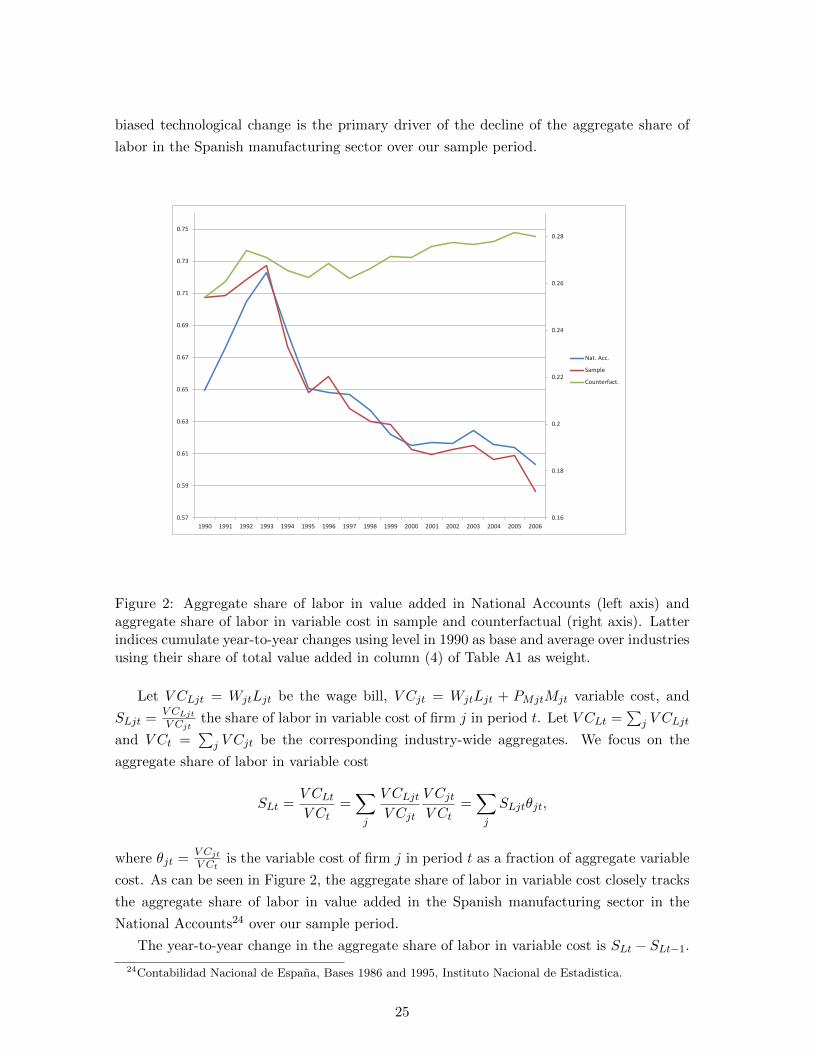
Figure 2: Aggregate share of labor in value added in National Accounts (left axis) andaggregate share of labor in variable cost in sample and counterfactual (right axis). Latterindices cumulate year-to-year changes using level in 1990 as base and average over industriesusing their share of total value added in column (4) of Table A1 as weight.

Let V CLjt = WjtLjt be the wage bill, V Cjt = WjtLjt + PMjtMjt variable cost, and

SLjt =V CLjtV Cjt

the share of labor in variable cost of firm j in period t. Let V CLt =∑

j V CLjt

and V Ct =∑

j V Cjt be the corresponding industry-wide aggregates. We focus on the

aggregate share of labor in variable cost

SLt =V CLtV Ct

=∑j

V CLjtV Cjt

V CjtV Ct

=∑j

SLjtθjt,

where θjt =V CjtV Ct

is the variable cost of firm j in period t as a fraction of aggregate variable

cost. As can be seen in Figure 2, the aggregate share of labor in variable cost closely tracks

the aggregate share of labor in value added in the Spanish manufacturing sector in the

National Accounts24 over our sample period.

The year-to-year change in the aggregate share of labor in variable cost is SLt − SLt−1.

24Contabilidad Nacional de Espana, Bases 1986 and 1995, Instituto Nacional de Estadistica.

25

Cumulated over our sample period, the decline of the aggregate share of labor ranges from

0.01 and 0.05 in industries 9 and 4 to 0.15 and 0.19 in industries 2 and 5, as can be seen in

column (1) of Table 6.25 To obtain insight into this decline, we build on Oberfield & Raval

(2014) and decompose the year-to-year change as

SLt − SLt−1 =∑j

θjt(SLjt − SLjt−1) +∑j

(θjt − θjt−1)SLjt−1.

The second term captures reallocation across firms. Our model enables us to further de-

compose the first term. Rewriting equation (10) yields

SLjt =1

1 + exp (−γL + (1− σ) (pMjt − wjt + ωLjt) + σλ2(STjt)− (1− σ)γ1(SOjt)). (17)

The first term may thus be driven by a change in the price of materials pMjt relative to

the price of labor wjt, a change in labor-augmenting productivity ωLjt, a change in the

share of temporary labor STjt, and a change in the share of outsourced materials SOjt. To

quantify these drivers, we use a second-order approximation to SLjt − SLjt−1 as described

in Appendix F.

We report the decomposition of the year-to-year change, cumulated over our sample

period, in columns (2)–(7) of Table 6. The small size of the residual in column (7) indicates

that our second-order approximation to SLjt−SLjt−1 readily accommodates nonlinearities.

As can be seen in column (3), biased technological change emerges as the main force behind

the decline of the aggregate share of labor. Changes in input prices in column (2) attenuate

the decline. In contrast, the impact of temporary labor, outsourced materials, and reallo-

cation across firms in the remaining columns is sometimes positive and sometimes negative

and mostly small.

We use our model to compute the counterfactual evolution of the aggregate share of

labor absent biased technological change by zeroing out the change in labor-augmenting

productivity ωLjt in the decomposition of the year-to-year change. As can be seen in

Figure 2, absent biased technological change the aggregate share of labor remains roughly

constant over our sample period. We emphasize that this counterfactual holds fixed not

only reallocation across firms but also the evolution of input prices, temporary labor, and

outsourced materials. This may be questionable over longer stretches of time.

Our conclusion that biased technological change is the primary driver of the decline of

the aggregate share of labor echoes that of Oberfield & Raval (2014). Oberfield & Raval

(2014) develop a decomposition of the change in the aggregate share of labor in value added

in the U.S. manufacturing sector from 1970 to 2010. Perhaps the most important difference

between their decomposition and ours is that we directly measure the bias of technological

25We estimate SLt − SLt−1 as well as the various terms of the decomposition using firms that are in thesample in periods t and t− 1.

26

change at the level of the individual firm, whereas Oberfield & Raval (2014) treat it as the

residual of their decomposition. Despite this difference and the different data sets used,

the decompositions are complementary and both point to the overwhelming role of biased

technological change in the decline of the aggregate share of labor.

8 Hicks-neutral technological change

From equation (12) we obtain an estimate of the elasticity of substitution and recover labor-

augmenting productivity at the firm level. To recover Hicks-neutral productivity and the

remaining parameters of the production function, we have to estimate equation (15).

Distributional parameters and elasticity of scale. Table 7 reports the distributional

parameters βK and βM = 1− βK and the elasticity of scale ν. Our estimates of βK range

from 0.07 in industry 8 to 0.31 in industry 6 (column (1)). Although the estimates of the

elasticity of scale are rarely significantly different from one, taken together they suggest

slightly decreasing returns to scale (columns (2)). We cannot reject the validity of the

moment conditions in any industry by a wide margin (columns (3) and (4)).26

Price elasticity. Column (5) of Table 7 reports the average absolute value of the price

elasticity η(pjt−1, Djt−1) implied by our estimates. It ranges from 1.79 in industry 9 to 6.04

and 9.11 in industries 5 and 2 and averages 3.20 across industries.27

Elasticity of substitution: Lagrange-multiplier test. The production function in

equation (6) assumes that the elasticity of substitution between capital, labor, and mate-

rials is the same. We compare our leading specification to the more general nested CES

production function

Yjt =

βKK −(1−τ)τ

jt +

[(exp(ωLjt)L

∗jt

)−(1−σ)σ + βM

(M∗jt

)−(1−σ)σ

] −σ1−σ

−(1−τ)τ

−ντ1−τ

exp(ωHjt) exp(ejt),

where the additional parameter τ is the elasticity of substitution between capital and labor,

respectively, materials. We show in the Online Appendix that our first estimation equation

(12) remains unchanged and generalize our second estimation equation (15). This allows us

to conduct a Lagrange-multiplier test for τ = σ. As can be seen in columns (6) and (7) of

Table 7, we cannot reject the validity of our leading specification in any industry.

26In light of this wide margin, we do not further probe the validity of lagged prices as instruments.27For U.S. manufacturing industries, Oberfield & Raval (2014) report price elasticities in a somewhat

narrower range between 2.91 and 5.22 with a roughly comparable average of 3.91 across industries.

27

Hicks-neutral technological change. With equation (15) estimated, we recover the

Hicks-neutral productivity ωHjt of firm j in period t up to an additive constant from equa-

tion (11); in what follows, we use ωHjt to denote the de-meaned Hicks-neutral productivity.

We proceed as before to obtain aggregate measures representing an industry.

The growth of Hicks-neutral productivity at firm j in period t is ∆ωHjt = ωHjt−ωHjt−1.

Ceteris paribus ∆ωHjt ≈X− νσ

1−σjt−1 exp(ωHjt) exp(ejt−1)−X

− νσ1−σ

jt−1 exp(ωHjt−1) exp(ejt−1)

X− νσ

1−σjt−1 exp(ωHjt−1) exp(ejt−1)

approximates

the rate of growth of a firm’s output Yjt−1 and is therefore directly comparable to the output

effect of labor-augmenting technological change. As can be seen from column (1) of Table

8, Hicks-neutral productivity grows quickly in five industries, with rates of growth ranging,

on average, from 1.2% per year in industry 8 to 4.4% in industry 1. It grows much more

slowly or barely at all in three industries, with rates of growth below 0.5% per year. While

there is considerable heterogeneity in the rate of growth of Hicks-neutral productivity across

industries, Hicks-neutral technological change causes output to grow by 1.4% per year.

0.75

1

1.25

1.5

1.75

1991 1992 1993 1994 1995 1996 1997 1998 1999 2000 2001 2002 2003 2004 2005 2006

Metals

Minerals

Chemical

Machinery

Electrical

Transport

Food

Textile

Timber

Paper

Figure 3: Hicks-neutral technological change. Index normalized to one in 1991.

Figure 3 illustrates the magnitude of Hicks-neutral technological change. The depicted

index cumulates the year-to-year changes and is normalized to one in 1991.28 The hetero-

geneity in the impact of Hicks-neutral technological change across industries clearly exceeds

28In industry 9, in line with column (1) of Table 8, we trim values of ∆ωH below −0.25 and above 0.5.

28

that of the output effect of labor-augmenting technological change (see again Figure 1).

Once again, technological change appears to have slowed in the 2000s compared to the

1990s: across industries, Hicks-neutral technological change causes output to grow by 2.7%

per year before 2000 and to shrink by 0.6% per year after 2000.

Dispersion and persistence. We measure dispersion by the interquartile range of ωHjt.

As can be seen from column (2) of Table 8, the interquartile range is between 0.37 in

industry 3 and 0.98 in industry 4.29 Hicks-neutral productivity appears to be somewhat

more disperse than labor-augmenting productivity in output terms. Once again, ωHjt is

highly autocorrelated (column (3)), indicating that differences in Hicks-neutral productivity

between firms persist over time.

Firms’ R&D activities. As can be seen from column (4) of Table 8, firms that per-

form R&D have, on average, higher levels of Hicks-neutral productivity than firms that do

not perform R&D in six industries but lower levels of Hicks-neutral productivity in four

industries. While there is practically no difference in industry 10, the rate of growth of

Hicks-neutral productivity for firms that perform R&D, on average, exceeds that of firms

that do not perform R&D in five industries (columns (5) and (6)). Overall, our estimates

indicate that firms’ R&D activities are associated with higher levels and rates of growth of

Hicks-neutral productivity, although firms’ R&D activities seem less closely tied to Hicks-

neutral than to labor-augmenting productivity. This is broadly consistent with the large

literature on induced innovation that argues that firms direct their R&D activities to con-

serve the relatively more expensive factors of production, in particular labor.30

Firm turnover. Similar to the output effect of labor-augmenting technological change,

survivors account for most of Hicks-neutral technological change. Their contribution is 61%

in industry 9 and above. While the contributions of entrants and exitors are small in most

industries, they are negative and more sizable in industries 2, 5, 7, 8, and 10. As a result, in

these industries the rate of growth of Hicks-neutral productivity is 0.7%, 3.0%, 1.2%, 1.7%,

and 1.2% amongst surviors compared to 0.5%, 2.0%, 0.1%, 1.2%, and 0.2% for all firms (see

again column (1) of Table 8).

Total technological change and its components. As productivity is multi-dimensional,

we take total technological change to be εLjt−2∆ωLjt + ∆ωHjt. Taken together, labor-

augmenting and Hicks-neutral technological change cause output to grow by, on average,

between 0.7% in industry 7 and 7.2% and 7.8% in industries 4 and 6, as can be seen in

29For Chinese manufacturing industries, Hsieh & Klenow (2009) report an interquartile range of log totalfactor productivity of 1.28.

30More explicitly testing for induced innovation is difficult because we do not observe what a firm doeswith its R&D expenditures. One way to proceed may be to add interactions of R&D expenditures and inputprices to the laws of motion in equations (7) and (8). We leave this to future research.

29

column (7) of Table 8. Across all industries, total technological change causes output to

grow by 3.1% per year.

The output effect of labor-augmenting technological change εLjt−2∆ωLjt and Hicks-

neutral technological change ∆ωHjt are positively correlated in nine industries while the

correlation is slightly negative in one industry (column (8)). The correlation between labor-

augmenting productivity in output terms εLjt−2ωLjt and Hicks-neutral productivity ωHjt is

positive in all industries. Overall, our estimates not only provide evidence that productivity

is multi- instead of single-dimensional but also suggest that the various components of

productivity are intertwined.

9 An aggregate productivity growth decomposition

In quantifying labor-augmenting and Hicks-neutral technological change in Sections 6 and

8, we leverage our firm-level panel data to follow individual firms over time. In this section,

we complement our findings by analyzing the aggregate productivity of the Spanish manu-

facturing sector and its growth over our sample period. To obtain insight into the drivers

of growth, we decompose aggregate productivity growth along the lines of Olley & Pakes

(1996).

Aggregate productivity φt =∑

j µjtφjt in period t is a weighted average of the produc-

tivity of individual firms, where φjt is a measure of the productivity of firm j in period

t and µjt is its weight. We separately examine labor-augmenting productivity in output

terms εLjt−2ωLjt, Hicks-neutral productivity ωHjt, and total productivity εLjt−2ωLjt+ωHjt.

Throughout the weight µjt = (pjt+yjt)/∑

j(pjt+yjt) is the share of the log of sales of firm

j in period t.

The growth in aggregate productivity from period t1 to period t2 is ∆φ = φt2 − φt1 .

Following Olley & Pakes (1996) and Melitz & Polanec (2015), we decompose this growth as

∆φ = ∆φS + µEt2(φEt2 − φ

St2

)+ µXt1

(φSt1 − φ

Xt1

)= ∆φ

S+NS∆Cov

(µ

µS, φ

)+ µEt2

(φEt2 − φ

St2

)+ µXt1

(φSt1 − φ

Xt1

), (18)

where S, E, and X indexes the group of survivors, entrants, and exitors, respectively.

µGt =∑

j∈G µjt is the total weight of group G in period t, φGt =∑

j∈GµjtµGtφjt is the

weighted average restricted to group G, φGt = 1

NG

∑j∈G φjt is the unweighted average

restricted to group G, NG is the number of firms in group G, and ∆Cov(µµS, φ)

is short for

Cov

(µjt2µSt2

, φjt2

)− Cov

(µjt1µSt1

, φjt1

). In the first line of the decomposition, the first term

captures the contribution of survivors to aggregate productivity growth, the second that of

entrants, and the third that of exitors. The second line further decomposes the contribution

of survivors to aggregate productivity growth into a shift in the distribution of productivity

30

(first term) and a change in covariance that captures reallocation (second term).

As the decomposition pertains to the population of firms, applying it to the sample

of firms in our firm-level panel data is subject to a caveat. As before we account for the

survey design by replicating the subsample of small firms. We classify a firm as a survivor

if it enters the industry in or before period t1 and does not exit in or before period t2. We

further classify a firm as an entrant if it enters the industry after period t1 and as an exitor

if it exits the industry in or before period t2. Due to attrition and the periodic addition

of new firms to the sample, we observe productivity for a subset of survivors in period t1

and for another subset of survivors in period t2. Because we average over potentially quite

different subsets of firms, especially if periods t1 and t2 are far apart, our estimates of the

various terms in the decomposition may be noisy.

We report the change in aggregate productivity and its decomposition in Table 9 for

the period 1992 to 2006 and the three subperiods 1992 to 1996, 1997 to 2001, and 2002

to 2006. The change in aggregate productivity in column (1) in Table 9 is consistent with

our findings in Sections 6 and 8. Aggregate labor-augmenting productivity in output terms

grew by 21.7% for the period 1992 to 2006 or about 1.6% per year. Aggregate Hicks-neutral

productivity grew by 19.7% or about 1.4% per year and aggregate total productivity by

41.6% or about 3.0% per year. For the later subperiods, technological change appears to

have slowed down, in particular in case of aggregate Hicks-neutral and total productivity.

We report the various terms of the decomposition in the first line of equation (18) in

columns (2), (5), and (6) of Table 9 and those in the second line in columns (3), (4), (5),

and (6). Turning to columns (2), (5), and (6), survivors account for most of the change in

aggregate total productivity and its components, again in line with our findings in Sections

6 and 8.31 With the possible exception of entrants for the subperiod 1992 to 1996, the

contribution of entrants and exitors appears to be limited. Honing in on survivors and

further decomposing their contribution, shifts in the distribution of productivity in column

(3) are substantially more important than changes on the covariance in column (4). The

contribution of reallocation to the change in aggregate total productivity and its components

is sometimes positive and sometimes negative and mostly small.

10 Capital-augmenting technological change

As discussed in Section 3, the evolution of the relative quantities and prices of the various

factors of production provides no evidence for capital-augmenting technological change.

Our leading specification therefore restricts the productivities of capital and materials to

change at the same rate and in lockstep with Hicks-neutral technological change. A more

general specification allows for capital-augmenting productivity ωKjt so that the production

31Survivors account for less of the change for the period 1992 to 2006 than for the three subperiods simplybecause the definition of survivor is more demanding if periods t1 and t2 are further apart.

31

function in equation (6) becomes

Yjt =[βK (exp(ωKjt)Kjt)

− 1−σσ +

(exp(ωLjt)L

∗jt

)− 1−σσ + βM

(M∗jt

)− 1−σσ

]− νσ1−σ

exp(ωHjt) exp(ejt).

(19)

We explore the role of capital-augmenting technological change in our data in two ways.

First, we follow Raval (2013) and parts of the previous literature on estimating aggregate

production functions (see Antras (2004) and the references therein) and assume that capital

is a static input that is chosen each period to maximize short-run profits. In analogy to

equation (10), we recover (conveniently rescaled) capital-augmenting productivity ωKjt =

(1− σ)ωKjt as

ωKjt = γK +mjt − kjt + σ(pMjt − pKjt) + (1− σ)γ1(SOjt)

≡ hK(mjt − kjt, pMjt − pKjt, SOjt), (20)

where γK = −σ ln(βMβK

)and we use the user cost in our data as a rough measure of the

price of capital pKjt. Using our leading estimates from Section 6, we recover the capital-

augmenting productivity ωKjt =ωKjt1−σ of firm j in period t up to an additive constant;

in what follows, we use ωKjt to denote the de-meaned capital-augmenting productivity.32

∆ωKjt ≈exp(ωKjt)Kjt−1−exp(ωKjt−1)Kjt−1

exp(ωKjt−1)Kjt−1in column (1) of Table 10 approximates the rate of

growth of a firm’s effective capital stock exp(ωKjt−1)Kjt−1 and εKjt−2∆ωKjt in column (2)

the rate of growth of the firm’s output Yjt−1, where εKjt−2 is the elasticity of output with

respect to the firm’s effective capital stock (see Appendix E). As can be seen from column

(1), capital-augmenting productivity grows slowly, on average, with rates of growth of 0.8%

per year in industry 6, 2.2% in industry 10, and 5.6% in industry 1. The rate of growth is

negative in the remaining seven industries. The growth of capital-augmenting productivity

is especially underwhelming in comparison to the growth of labor-augmenting productivity

(see again column (1) of Table 5). The output effect of capital-augmenting technological

change in column (2) is also close to zero in all industries, although this likely reflects the

fact that capital is not a static input. As the user cost excludes adjustment costs, it falls

short of the shadow price of capital, and using it drives down the elasticity of output with

respect to the firm’s effective capital stock.

Second, we return to the usual setting in the literature following Olley & Pakes (1996)

and allow the choice of capital to have dynamic implications. We follow parts of the previous

literature on estimating aggregate production functions and proxy for ωKjt by a time trend

32As an alternative to plugging our leading estimates from Section 6 into equation (20), in the OnlineAppendix we use equation (20) to form the analog to our first estimation equation (12):

mjt − kjt = −σ(pMjt − pKjt)− (1− σ)γ1(SOjt)

+gKt−1(hK(mjt−1 − kjt−1, pMjt−1 − pKjt−1, SOjt−1), Rjt−1) + ξKjt.

Consistent with measurement error in pKjt, the resulting estimates of σ are very noisy and severely biasedtoward zero.

32

δKt. Our second estimation equation (15) remains unchanged except that

Xjt = βK (exp(δKt)Kjt)− 1−σ

σ + βM (Mjt exp (γ1(SOjt)))− 1−σ

σ

(1− SMjt

SMjtλ1(STjt) + 1

).

Columns (3)–(7) of Table 10 summarize the resulting estimates of βK , ν, and δK . The

estimates of βK and ν are very comparable to those in Table 5. Moreover, the insignificant

time trend leaves little room for capital-augmenting technological change in our data.

In sum, in line with the patterns in the data described in Section 3, there is little, if

any, evidence for capital-augmenting technological change in our data. Of course, our ways

of exploring the role of capital-augmenting technological change are less than ideal in that

they either rest on the assumption that capital is a static input or abstract from firm-

level heterogeneity in capital-augmenting productivity. An important question is therefore

whether our approach can be extended to treat capital-augmenting productivity on par

with labor-augmenting and Hicks-neutral productivity.

Recovering a third component of productivity, at a bare minimum, requires a third

decision besides labor and materials to invert. Investment is a natural candidate. In contrast

to the demand for labor and materials, however, investment depends on the details of the

firm’s dynamic programming problem. There are two principal difficulties. First, one has

to prove that the observed demands for labor and materials along with investment are

jointly invertible for unobserved capital-augmenting, labor-augmenting, and Hicks-neutral

productivity. Second, the inverse functions hK(·), hL(·), and hH(·) are high-dimensional.

Thus, estimating these functions nonparametrically is demanding on the data. In ongoing

work, Zhang (2015) proposes combining a parametric inversion that exploits the parameter

restrictions between production and input demand functions similar to our paper with a

nonparametric inversion of investment similar to Olley & Pakes (1996).

11 Conclusions

Technological change can increase the productivity of capital, labor, and the other factors

of production in equal terms, or it can be biased towards a specific factor. In this paper, we

directly assess the bias of technological change by measuring, at the level of the individual

firm, how much of technological change is labor augmenting and how much of it is Hicks

neutral.

To this end, we develop a dynamic model of the firm in which productivity is multi-

dimensional. At the center of the model is a CES production function that parsimoniously

yet robustly relates the relative quantities of materials and labor to their relative prices and

labor-augmenting productivity. To properly isolate and measure labor-augmenting produc-

tivity, we account for other factors that impact this relationship, in particular, outsourcing

and adjustment costs on permanent labor.

33

We apply our estimator to an unbalanced panel of 2375 Spanish manufacturing firms in

ten industries from 1990 to 2006. Our estimates indicate limited substitutability between

the various factors of production. This calls into question whether the widely-used Cobb-

Douglas production function with its unitary elasticity of substitution adequately represents

firm-level production processes.

Our estimates provide clear evidence that technological change is biased. Ceteris paribus

labor-augmenting technological change causes output to grow, on average, in the vicinity

of 1.5% per year. While skill upgrading explains some of the growth of labor augmenting

productivity, in many industries labor-augmenting productivity grows because workers with

a given set of skills become more productive over time. In short, our estimates cast doubt on

the assumption of Hicks-neutral technological change that underlies many of the standard

techniques for measuring productivity and estimating production functions.

At the same time, however, our estimates do not validate the assumption that tech-

nological change is purely labor augmenting that plays a central role in the literature on

economic growth. In addition to labor-augmenting technological change, our estimates show

that Hicks-neutral technological change causes output to grow, on average, in the vicinity

of 1.5% per year.

While we are primarily interested in measuring how much of technological change is la-

bor augmenting and how much of it is Hicks neutral, we also use our estimates to illustrate

the consequences of biased technological change beyond the growth of output. In particu-

lar, we show that it is the primary driver of the decline of the aggregate share of labor in

the Spanish manufacturing sector over our sample period. An interesting avenue for future

research is to investigate the implications of biased technological change for employment.

Recent research points to biased technological change as a key driver of the diverging expe-

riences of the continental European, U.S., and U.K. economies during the 1980s and 1990s

(Blanchard 1997, Caballero & Hammour 1998, Bentolila & Saint-Paul 2004, McAdam &

Willman 2013). Our estimates lend themselves to decomposing firm-level changes in em-

ployment into displacement, substitution, and output effects and to compare these effects

between labor-augmenting and Hicks-neutral technological change. This may be helpful for

better understanding and predicting the evolution of employment as well as for designing

labor market and innovation policies in the presence of biased technological change.

Appendix A Proof of proposition 1

Rewriting the ratio of first-order conditions (3) yields

0 = ln∂H (exp(ωLjt − (mjt − ljt)), 1)

∂Ljt+ ωLjt − ln

∂H (exp(ωLjt − (mjt − ljt)), 1)

∂Mjt+ pMjt − wjt

= f(mjt − ljt, pMjt − wjt, ωLjt).

34

Differentiating the so-defined function f(·) yields

∂f(mjt − ljt, pMjt − wjt, ωLjt)∂(mjt − ljt)

=

−∂2H(exp(ωLjt−(mjt−ljt)),1)

∂L2jt

∂H(exp(ωLjt−(mjt−ljt)),1)∂Ljt

+

∂2H(exp(ωLjt−(mjt−ljt)),1)∂Mjt∂Ljt

∂H(exp(ωLjt−(mjt−ljt)),1)∂Mjt

exp(ωLjt − (mjt − ljt))

=H (exp(ωLjt − (mjt − ljt)), 1)

∂2H(exp(ωLjt−(mjt−ljt)),1)∂Mjt∂Ljt

∂H(exp(ωLjt−(mjt−ljt)),1)∂Ljt

∂H(exp(ωLjt−(mjt−ljt)),1)∂Mjt

=1

σ (exp(ωLjt − (mjt − ljt))),

where the second equality uses that H(exp(ωLjt)Ljt,Mjt) is homogeneous of degree oneand the third equality uses that the elasticity of substitution between materials and labor(Chambers 1988, equation (1.13)) for the production function in equation (1) simplifies to

σ (exp(ωLjt − (mjt − ljt))) =

∂H(exp(ωLjt−(mjt−ljt)),1)∂Ljt

∂H(exp(ωLjt−(mjt−ljt)),1)∂Mjt

H (exp(ωLjt − (mjt − ljt)), 1)∂2H(exp(ωLjt−(mjt−ljt)),1)

∂Mjt∂Ljt

.

Similarly,

∂f(mjt − ljt, pMjt − wjt, ωLjt)∂(pMjt − wjt)

= 1,

∂f(mjt − ljt, pMjt − wjt, ωLjt)∂ωLjt

= − 1

σ (exp(ωLjt − (mjt − ljt)))+ 1.

By the implicit function theorem, around a point (m0jt − l0jt, p

0Mjt − w0

jt, ω0Ljt) satisfying

f(m0jt−l0jt, p0

Mjt−w0jt, ω

0Ljt) = 0, there exists a continuously differentiable functionmjt−ljt =

g(pMjt − wjt, ωLjt) such that f(g(pMjt − wjt, ωLjt), pMjt − wjt, ωLjt) = 0 and

∂g(p0Mjt − w0

jt, ω0Ljt)

∂(pMjt − wjt)= −

∂f(m0jt−l0jt,p0

Mjt−w0jt,ω

0Ljt)

∂(pMjt−wjt)∂f(m0

jt−l0jt,p0Mjt−w

0jt,ω

0Ljt)

∂(mjt−ljt)

= −σ(exp(ω0

Ljt − (m0jt − l0jt))

),

∂g(p0Mjt − w0

jt, ω0Ljt)

∂ωLjt= −

∂f(m0jt−l0jt,p0

Mjt−w0jt,ω

0Ljt)

∂ωLjt

∂f(m0jt−l0jt,p0

Mjt−w0jt,ω

0Ljt)

∂(mjt−ljt)

= 1− σ(exp(ω0

Ljt − (m0jt − l0jt))

).

The first-order Taylor series for mjt − ljt = g(pMjt − wjt, ωLjt) around the point (m0jt −

l0jt, p0Mjt − w0

jt, ω0Ljt) follows immediately.

Appendix B Data

We observe firms for a maximum of 17 years between 1990 and 2006. We restrict thesample to firms with at least three years of data on all variables required for estimation.The number of firms with 3, 4,. . . , 17 years of data is 313, 240, 218, 215, 207, 171, 116,189, 130, 89, 104, 57, 72, 94, and 160, respectively. Table A1 gives the industry definitions

35

along with their equivalent definitions in terms of the ESEE, National Accounts, and ISICclassifications (columns (1)–(3)). Based on the National Accounts in 2000, we further reportthe shares of the various industries in the total value added of the manufacturing sector(column (4)).

In what follows we define the variables we use for our main analysis.

• Investment. Value of current investments in equipment goods (excluding buildings,land, and financial assets) deflated by the price index of investment. The price ofinvestment is the equipment goods component of the index of industry prices computedand published by the Spanish Ministry of Industry.

• Capital. Capital at current replacement values Kjt is computed recursively from

an initial estimate and the data on current investments in equipment goods Ijt. Weupdate the value of the past stock of capital by means of the price index of investmentPIt as Kjt = (1− δ) PIt

PIt−1Kjt−1 + Ijt−1, where δ is an industry-specific estimate of the

rate of depreciation. Capital in real terms is obtained by deflating capital at current

replacement values by the price index of investment as Kjt =KjtPIt

.

• Labor. Total hours worked computed as the number of workers times the averagehours per worker, where the latter is computed as normal hours plus average overtimeminus average working time lost at the workplace.

• Materials. Value of intermediate goods consumption (including raw materials, com-ponents, energy, and services) deflated by a firm-specific price index of materials.

• Output. Value of produced goods and services computed as sales plus the variation ofinventories deflated by a firm-specific price index of output.

• Wage. Hourly wage cost computed as total labor cost including social security pay-ments divided by total hours worked.

• Price of materials. Firm-specific price index for intermediate consumption. Firmsare asked about the price changes that occurred during the year for raw materials,components, energy, and services. The price index is computed as a Paasche-typeindex of the responses.

• Price of output. Firm-specific price index for output. Firms are asked about theprice changes they made during the year in up to five separate markets in which theyoperate. The price index is computed as a Paasche-type index of the responses.

• Demand shifter. Firms are asked to assess the current and future situation of themain market in which they operate. The demand shifter codes the responses as 0,0.5, and 1 for slump, stability, and expansion, respectively.

• Share of temporary labor. Fraction of workers with fixed-term contracts and no orsmall severance pay.

• Share of outsourcing. Fraction of customized parts and pieces that are manufacturedby other firms in the value of the firm’s intermediate goods purchases.

36

• R&D expenditures. R&D expenditures include the cost of intramural R&D activi-ties, payments for outside R&D contracts with laboratories and research centers, andpayments for imported technology in the form of patent licensing or technical assis-tance, with the various expenditures defined according to the OECD Oslo and Frascatimanuals.

We next turn to additional variables that we use for descriptive purposes, extensions, androbustness checks.

• User cost of capital. Computed as PIt(rjt + δ−CPIt), where PIt is the price index ofinvestment, rjt is a firm-specific interest rate, δ is an industry-specific estimate of therate of depreciation, and CPIt is the rate of inflation as measured by the consumerprice index.

• Skill mix. Fraction of non-production employees (white collar workers), workers withan engineering degree (engineers), and workers with an intermediate degree (techni-cians). Available in the year a firm enters the sample and every subsequent four years;assumed to be unchanging in the interim.

• Region. Dummy variables corresponding to the 19 Spanish autonomous communitiesand cities where employment is located if it is located in a unique region and anotherdummy variable indicating that employment is spread over several regions.

• Product submarket. Dummy variables corresponding to a finer breakdown of the 10industries into subindustries (restricted to subindustries with at least five firms, seecolumn (5) of Table A1).

• Technological sophistication. Dummy variable that takes the value one if the firmuses digitally controlled machines, robots, CAD/CAM, or some combination of theseprocedures.

• Identification between ownership and control. Dummy variable that takes the valueone if the owner of the firm or the family of the owner hold management positions.

• Age. Years elapsed since the foundation of the firm with a maximum of 40 years.

• Firm size. Number of workers in the year the firm enters the sample.

Appendix C Inverse functions

The first-order conditions for permanent and temporary labor are

νµX−(1+ νσ

1−σ )jt exp (ωHjt) exp

(−1− σ

σωLjt

)(L∗jt)− 1

σ∂L∗jt∂LPjt

=WPjt(1 + ∆jt)

Pjt

(1− 1

η(pjt,Djt)

) ,(21)

νµX−(1+ νσ

1−σ )jt exp (ωHjt) exp

(−1− σ

σωLjt

)(L∗jt)− 1

σ∂L∗jt∂LTjt

=WTjt

Pjt

(1− 1

η(pjt,Djt)

) ,(22)

where, by the envelope theorem, the gap between the wage of permanent workers WPjt andthe shadow wage is

∆jt =1

WPjt

(∂CLP (LPjt, LPjt−1)

∂LPjt− 1

1 + ρEt

[∂Vt+1(Ωjt+1)

∂LPjt|Ωjt, Rjt

])37

=1

WPjt

(∂CLP (LPjt, LPjt−1)

∂LPjt+

1

1 + ρEt

[∂CLP (LPjt+1, LPjt)

∂LPjt|Ωjt, Rjt

]).

Equations (21) and (22) allow the mix of permanent and temporary labor to depend on thefirm’s productivity and the other state variables (through ∆jt).

Our assumption that Λ(LPjt, LTjt) is linearly homogenous implies L∗jt = LjtΛ(1 −STjt, STjt),

∂L∗jt∂LPjt

= ΛP (1 − STjt, STjt), and∂L∗jt∂LTjt

= ΛT (1 − STjt, STjt). Using Euler’s

theorem to combine equations (21) and (22) yields

νµX−(1+ νσ

1−σ )jt exp (ωHjt) exp

(−1− σ

σωLjt

)L− 1σ

jt Λ(1− STjt, STjt)−1−σσ

=

Wjt

(1 +

∆jt

1+WTjtWPjt

STjt1−STjt

)Pjt

(1− 1

η(pjt,Djt)

) =

Wjt

(ΛP (1−STjt,STjt)ΛT (1−STjt,STjt)

+STjt

1−STjtWPjtWTjt

+STjt

1−STjt

)Pjt

(1− 1

η(pjt,Djt)

) , (23)

where the second equality follows from dividing equations (21) and (22) and solving for ∆jt.

Our assumption thatWPjt

WTjt= λ0 is an (unknown) constant implies that

ΛP (1−STjt,STjt)ΛT (1−STjt,STjt)

+STjt

1−STjt

λ0+STjt

1−STjt

=

λ1(STjt) as an (unknown) function of STjt.Turning from the labor to the materials decision, because the firm must maintain the ra-

tio of outsourced to in-house materials QMjt, the first-order condition for in-house materialsis

νβMµX−(1+ νσ

1−σ )jt exp (ωHjt)

(M∗jt

)− 1σdM∗jtdMIjt

=PMjt

Pjt

(1− 1

η(pjt,Djt)

) , (24)

where PMjt = PIjt+POjtQMjt is the effective cost of an additional unit of in-house materials.

Our assumption that Γ(MIjt,MOjt) is linearly homogenous impliesM∗jt = MIjtΓ(

1,PIjtPOjt

SOjt1−SOjt

)and

dM∗jtdMIjt

= Γ(

1,PIjtPOjt

SOjt1−SOjt

). Rewriting equation (24) yields

νβMµX−(1+ νσ

1−σ )jt exp (ωHjt)M

− 1σ

jt Γ

(1,PIjtPOjt

SOjt1− SOjt

)− 1−σσ

=PMjt

Pjt

(1− 1

η(pjt,Djt)

) . (25)

Our assumption thatPIjtPOjt

= γ0 is an (unknown) constant implies that ln Γ(

1, γ0SOjt

1−SOjt

)=

γ1(SOjt) as an (unknown) function of SOjt.33

Solving equations (23) and (25) for ωLjt = (1 − σ)ωLjt and ωHjt yields equations (10)

and (11), where λ2(STjt) = ln(λ1(STjt)Λ (1− STjt, STjt)

1−σσ

).

33Equation (25) presumes an interior solution for in-house materials; it is consistent with a corner solutionfor outsourced materials. Indeed, absent outsourcing equation (25) reduces to the first-order condition forin-house materials.

38

Appendix D Estimation

Unknown functions. The functions gL1(hL(·)), gL2(hL(·), rjt−1), gH1(hH(·)), and gH2(hH(·), rjt−1)

that are part of the conditional expectation functions gLt−1(hL(·), Rjt−1) and gHt−1(hH(·), Rjt−1)are unknown and must be estimated nonparametrically, as must be the absolute value ofthe price elasticity η(pjt, Djt) and the correction terms λ1(STjt), λ2(STjt), and γ1(SOjt).We model an unknown function q(v) of one variable v by a univariate polynomial of degreeQ. We model an unknown function q(u, v) of two variables u and v by a complete set ofpolynomials of degree Q. Unless otherwise noted, we omit the constant in q(·) and setQ = 3 in the remainder of this paper.

Starting with the conditional expectation functions, we specify gL1(hL(·)) = q(hL(·) −γL), gL2(hL(·), rjt) = q0+q(hL(·)−γL, rjt), gH1(hH(·)) = q(hH(·)−γH), and gH2(hH(·), rjt) =q0 + q(hH(·)− γH , rjt), where q0 is a constant and the function q(·) is modeled as describedabove. Without loss of generality, we absorb γL and γH into the overall constants of our esti-mation equations. Turning to the absolute value of the price elasticity, to impose the theoret-ical restriction η(pjt, Djt) > 1, we specify η(pjt, Djt) = 1 + exp(q(pjt, Djt)), where the func-tion q(·) is modeled as described above except that we suppress terms involving D2

jt and D3jt.

Turning to the correction terms, we specify λ1(STjt) = q(lnSTjt) and λ2(STjt) = q(lnSTjt)in industries 2, 3, and 10 and λ1(STjt) = q(ln(1 − STjt)) and λ2(STjt) = q(ln(1 − STjt))in the remaining industries.34 Finally, we specify γ1(SOjt) = q(SOjt); this ensures thatγ1(SOjt) = 0 if SOjt = 0 in line with the normalization Γ(MIjt, 0) = MIjt.

Parameters and instruments. Our first estimation equation (12) has 36 parameters:constant, σ, 15 parameters in gL0(t − 1) (time dummies), 3 parameters in gL1(hL(·)), 10parameters in gL2(hL(·), rjt−1), 3 parameters in λ2(STjt), and 3 parameters in γ1(SOjt).

Our instrumenting strategy is adapted from Doraszelski & Jaumandreu (2013) andwe refer the reader to Doraszelski & Jaumandreu (2013) and the references therein fora discussion of the use of polynomials for instruments. We use the constant, 15 timedummies, the dummy for performers 1(Rjt−1 > 0), the demand shifter Djt, and a univariatepolynomial in lnSOjt−1 +mjt−1 interacted with 1(SOjt−1 > 0) (3 instruments). We furtheruse a complete set of polynomials in ljt−1, mjt−1, and pMjt−1 − wjt−1 interacted with thedummy for nonperformers 1(Rjt−1 = 0) (19 instruments). In industries 5 and 8 we replacepMjt−1 − wjt−1 by pMjt−1 in the complete set of polynomials. Finally, we use a completeset of polynomials in ljt−1, mjt−1, and pMjt−1−wjt−1 and rjt−1 interacted with the dummyfor performers 1(Rjt−1 > 0) (34 instruments). This yields a total of 74 instruments and74− 36 = 38 degrees of freedom (see column (4) of Table 4).

After imposing the estimated values from equation (12), our second estimation equation(15) has 40 parameters: constant, βK , ν, 15 parameters in gH0(t − 1) (time dummies),3 parameters in gH1(hH(·)), 10 parameters in gH2(hH(·), rjt−1), 3 parameters in λ1(STjt),and 6 parameters in η(pjt, Djt).

As before, we use polynomials for instruments. We use the constant, 15 time dummies,the dummy for performers 1(Rjt−1 > 0), the demand shifter Djt, a univariate polynomialin pjt−1 (3 instruments), a univariate polynomial in pMjt−1 − pjt−1 (3 instruments), and aunivariate polynomial in kjt (3 instruments). We also use a complete set of polynomials in

34To incorporate skill upgrading, we instead specify λ1(STjt,Θjt) = q(lnSTjt, ln Θjt) and λ2(STjt,Θjt) =q(lnSTjt, ln Θjt) in industries 2, 3, and 10 and λ1(STjt,Θjt) = q(ln(1 − STjt), ln Θjt) and λ2(STjt,Θjt) =q(ln(1 − STjt), ln Θjt) in the remaining industries, where the function q(·) is modeled as described aboveexcept that we suppress terms involving (ln Θjt)

2 and (ln Θjt)3.

39

Mjt−11−SMjt−1

SMjt−1and Kjt−1 interacted with the dummy for nonperformers 1(Rjt−1 = 0) (9

instruments). Finally, we use a complete set of polynomials in Mjt−11−SMjt−1

SMjt−1and Kjt−1 (9

instruments) and a univariate polynomial in rjt−1 interacted with the dummy for performers1(Rjt−1 > 0) (3 instruments). This yields a total of 48 instruments and 48− 40 = 8 degreesof freedom in industries 1, 2, 3, 6, 7, 9, and 10 (see column (3) of Table 7). In industries 4,5, and 8, we add a univariate polynomial in ln(1−STjt−1) (3 instruments). We replace theunivariate polynomial in kjt by kjt in industries 4 and 8 and we drop Djt in industry 5.

Estimation. From the GMM problem in equation (16) with weighting matrix WL =[1N

∑j ALj(zj)ALj(zj)

′]−1

we first obtain a consistent estimate θL of θL. This first step is

the NL2SLS estimator of Amemiya (1974). In the second step, we compute the optimal esti-

mate with weighting matrix WL =[

1N

∑j ALj(zj)νLj(θL)νLj(θL)

′ALj(zj)

′]−1

. Throughout

the paper, we report standard errors that are robust to heteroskedasticity and autocorrela-tion. We further correct standard errors as described in the Online Appendix to reflect thefact that our estimates of equation (15) are conditional on those of equation (12).

Implementation. Code for our estimator is available from the authors upon requestalong with instructions for obtaining the data. We use Gauss 14.0.9 and Optmum 3.1.7. Toreduce the number of parameters to search over in the GMM problem in equation (16), we“concentrate out” the parameters that enter it linearly as described in the Online Appendix.To guard against local minima, we have extensively searched over the remaining parameters,often using preliminary estimates to narrow down the range of these parameters.

Testing. The value of the GMM objective function for the optimal estimator, multipliedby N , has a limiting χ2 distribution with Q−P degrees of freedom, where Q is the numberof instruments and P the number of parameters to be estimated. We use it as a test foroveridentifying restrictions or validity of the moment conditions.

Appendix E Output effect

Direct calculation starting from equation (6) yields the elasticity of output with respect toa firm’s effective labor force:

εLjt =∂Yjt

∂ exp(ωLjt)L∗jt

exp(ωLjt)L∗jt

Yjt

=ν(

exp(ωLjt)L∗jt

)− 1−σσ

βKK− 1−σ

σjt +

(exp(ωLjt)L∗jt

)− 1−σσ

+ βM

(M∗jt

)− 1−σσ

. (26)

Using equation (10) to substitute for ωLjt and simplifying we obtain

εLjt =ν

1−SMjt

SMjtλ1(STjt)

βKβM

(Kjt

Mjt exp(γ1(SOjt))

)− 1−σσ

+1−SMjt

SMjtλ1(STjt) + 1

. (27)

40

Recall from equation (23) that λ1(STjt) = 1 +∆jt

1+WTjtWPjt

STjt1−STjt

, where ∆jt is the gap between

the wage of permanent workers WPjt and the shadow wage. To facilitate evaluating equation(27), we abstract from adjustment costs and set λ1(STjt) = 1.

Direct calculation starting from equation (19) also yields the elasticity of output withrespect to a firm’s effective capital stock:

εKjt =∂Yjt

∂ exp(ωKjt)Kjt

exp(ωKjt)Kjt

Yjt

=ν (exp(ωKjt)Kjt)

− 1−σσ

(exp(ωKjt)Kjt)− 1−σ

σ +(

exp(ωLjt)L∗jt

)− 1−σσ

+ βM

(M∗jt

)− 1−σσ

=ν

1 +PMjtMjt

PKjtKjt

(1−SMjt

SMjtλ1(STjt) + 1

) , (28)

where we use equations (10) and (20) to substitute for ωLjt and ωKjt, respectively. As withequation (27), we set λ1(STjt) = 1 to evaluate equation (28).

Appendix F Second-order approximation

Let Υjt = −γL + (1 − σ) (pMjt − wjt + ωLjt) + σλ2(STjt) − (1 − σ)γ1(SOjt) and ∆Υjt =Υjt −Υjt−1. Using equation (17) we write

SLjt − SLjt−1 = −SLjt(1− SLjt−1) (exp (∆Υjt)− 1)

≈ −SLjt(1− SLjt−1)

(∆Υjt +

1

2(∆Υjt)

2

),

where we replace exp (∆Υjt) − 1 by its second-order Taylor series approximation around∆Υjt = 0. We allocate the interactions in (∆Υjt)

2 in equal parts to the variables involved.

References

Acemoglu, Daron (2002), ‘Directed technical change’, Review of Economic Studies 69, 781–809.

Acemoglu, Daron (2003), ‘Labor- and capital-augmenting technical change’, Journal of theEuropean Economic Association 1(1), 1–37.

Ackerberg, Daniel, Benkard, C. Lanier, Berry, Steve & Pakes, Ariel (2007), Econometrictools for analyzing market outcomes, in James J. Heckman & Edward E. Leamer, eds,‘Handbook of Econometrics’, Vol. 6A, North-Holland, Amsterdam, pp. 4171–4276.

Ackerberg, Daniel, Caves, Kevin W. & Frazer, Garth (2015), ‘Identification properties ofrecent production function estimators’, Econometrica 83(6), 2411–2451.

Amemiya, Takeshi (1974), ‘The nonlinear two-stage least-squares estimator’, Journal ofEconomic Literature 2, 105–110.

41

Antras, Pol (2004), ‘Is the U.S. aggregate production function Cobb-Douglas? New esti-mates of the elasticity of substitution’, Contributions to Macroeconomics 4(1).

Atalay, Enghin (2014), ‘Materials prices and productivity’, Journal of the European Eco-nomic Association 12(3), 575–611.

Balat, Jorge F., Brambilla, Irene & Sasaki, Yuya (2015), Heterogeneous firms: Skilled-labor productivity and export destinations, Working paper, Johns Hopkins University,Baltimore.

Bartelsman, Eric J. & Doms, Mark E. (2000), ‘Understanding productivity: Lessons fromlongitudinal microdata’, Journal of Economic Literature 38(3), 569–594.

Bentolila, Samuel & Saint-Paul, Gilles (2004), ‘Explaining movements in the labor share’,Contributions to Macroeconomics 3(1).

Bernard, Andrew B., Redding, Steven J. & Schott, Peter K. (2010), ‘Multiple-product firmsand product switching’, American Economic Review 100(1), 70–97.

Binswanger, Hans P. (1974), ‘The measurement of technical change biases with many factorsof production’, American Economic Review 64(6), 964–976.

Blanchard, Olivier (1997), ‘The medium run’, Brookings Papers on Economic Activity:Macroecomomics 1997(2), 89–158.

Brown, Murray & de Cani, John S. (1963), ‘Technological change and the distribution ofincome’, International Economic Review 4(3), 289–309.

Bruno, Michael (1984), ‘Raw materials, profits, and the productivity slowdown’, QuarterlyJournal of Economics 99(1), 1–30.

Caballero, Ricardo J. & Hammour, Mohamad L. (1998), ‘Jobless growth: appropriabil-ity, factor substitution, and unemployment’, Carnegie-Rochester Conference Series onPublic Policy 48, 51–94.

Cain, Louis P. & Paterson, Donald G. (1986), ‘Biased technical change, scale, and factor sub-stitution in American industry, 1850-1919’, Journal of Economic History 46(1), 153–164.

Card, David & DiNardo, John E. (2002), ‘Skill-biased technological change and rising wageinequality: Some problems and puzzles’, Journal of Labor Economics 20(4), 733–783.

Chambers, Robert G. (1988), Applied production analysis: A dual approach, CambridgeUniversity Press, Cambridge.

Chirinko, Robert S. (2008), ‘σ: The long and short of it’, Journal of Multivariate Analysis30, 671–686.

David, Paul A. & van de Klundert, Theo (1965), ‘Biased efficiency growth and capital-laborsubstitution in the U.S., 1899-1960’, American Economic Review 55(3), 357–394.

Davis, Steven J. & Haltiwanger, John C. (1992), ‘Gross job creation, gross job destruction,and employment reallocation’, Quarterly Journal of Economics 107(3), 819–863.

42

De Loecker, Jan (2013), ‘Detecting learning by exporting’, American Economic Journal:Microeconomics 5(3), 1–21.

De Loecker, Jan, Goldberg, Pinelopi K., Khandelwal, Amit K. & Pavcnik, Nina (2016),‘Prices, markups and trade reform’, Econometrica 84(2), 445–510.

Dolado, Juan J., Garcia-Serrano, Carlos & Jimeno, Juan F. (2002), ‘Drawing lessons fromthe boom of temporary jobs in Spain’, Economic Journal 112(480), 270–295.

Doraszelski, Ulrich & Jaumandreu, Jordi (2013), ‘R&D and productivity: Estimating en-dogenous productivity’, Review of Economic Studies 80(4), 1338–1383.

Dunne, Timothy, Roberts, Mark J. & Samuelson, Larry (1988), ‘Patterns of firm entry andexit in U.S. manufacturing’, Rand Journal of Economics 19(4), 495–515.

Eslava, Marcela, Haltiwanger, John C., Kugler, Adriana & Kugler, Maurice (2004), ‘Theeffects of structural reforms on productivity and profitability enhancing reallocation:Evidence from Colombia’, Journal of Development Economics 75, 333–371.

European Commission (2001), ‘Statistics on innovation in Europe’, Enterprise DG, Brussels.

Foster, Lucia, Haltiwanger, John C. & Syverson, Chad (2008), ‘Reallocation, firm turnover,and efficiency: Selection on productivity or profitability?’, American Economic Review98(1), 394–425.

Foster, Lucia, Haltiwanger, John C. & Syverson, Chad (2016), ‘The slow growth of newplants: Learning about demand?’, Economica 83(329), 91–129.

Fox, Jeremy T., Haddad, Valentin, Hoderlein, Stefan, Petrin, Amil K. & Sherman, Robert P.(2016), Heterogeneous production functions, panel data, and productivity dispersion,Slide deck, Rice University, Houston.

Gandhi, Amit, Navarro, Salvador & Rivers, David A. (2013), On the identification of pro-duction functions: How heterogeneous is productivity?, Working paper, University ofWisconsin.

Goldberg, Pinelopi K., Khandelwal, Amit K., Pavcnik, Nina & Topalova, Petia B. (2010),‘Multiproduct firms and product turnover in the developing world: Evidence fromIndia’, Review of Economics and Statistics 92(4), 1042–1049.

Goldman, Steven M. & Uzawa, Hirofumi (1964), ‘A note on separability in demand analysis’,Econometrica 32(3), 387–398.

Grieco, Paul L., Li, Shengyu & Zhang, Hongsong (2016), ‘Production function estimationwith unobserved input price dispersion’, International Economic Review 57(2), 665–690.

Griliches, Zvi (1964), ‘Research expenditures, education and the aggregate agriculturalproduction function’, American Economic Review 54(6), 961–974.

Griliches, Zvi (1998), R&D and productivity: The econometric evidence, University ofChicago Press, Chicago.

43

Griliches, Zvi & Jorgenson, Dale W. (1967), ‘The explanation of productivity change’,Review of Economic Studies 34(3), 249–283.

Grossman, Gene M. & Helpman, Elhanan (2002), ‘Integration versus outsourcing in industryequilibrium’, Quarterly Journal of Economics 117(1), 85–120.

Grossman, Gene M. & Helpman, Elhanan. (2005), ‘Outsourcing in a global economy’, Re-view of Economic Studies 72(1), 135–159.

Hall, Robert E. (1988), ‘The relation between price and marginal cost in U.S. industry’,Journal of Political Economy 96(5), 921–947.

Hammermesh, Daniel S. (1993), Labor demand, Princeton University Press, Princeton.

Hansen, Lars P. (1982), ‘Large sample properties of generalized method of moments esti-mators’, Econometrica 50(4), 1029–1054.

Hicks, John R. (1932), The theory of wages, Macmillan, London.

Hsieh, Chang-Tai & Klenow, Peter J. (2009), ‘Misallocation and manufacturing TFP inChina and India’, Quarterly Journal of Economics 124(4), 1403–1448.

Jin, Hui & Jorgenson, Dale W. (2010), ‘Econometric modeling of technical change’, Journalof Econometrics 157(2), 205–219.

Jones, Charles I. (2005), ‘The shape of production functions and the direction of technicalchange’, Quarterly Journal of Economics 120(2), 517–549.

Kalt, Joseph P. (1978), ‘Technological change and factor substitution in the United States:1929- 1967’, International Economic Review 19(3), 761–775.

Karabarbounis, Loukas & Neiman, Brent (2014), ‘The global decline of the labor share’,Quarterly Journal of Economics 129(1), 61–103.

Kasahara, Hiroyuki & Rodrigue, Joel (2008), ‘Does the use of imported intermediatesincrease productivity? Plant-level evidence’, Journal of Development Economics87, 106–118.

Kasahara, Hiroyuki, Schrimpf, Paul & Suzuki, Michio (2015), Identification and estimationof production functions with unoberved heterogeneity, Working paper, University ofBritish Columbia, Vancouver.

Klump, Rainer, McAdam, Peter & Willman, Alpo (2007), ‘Factor substitution and factor-augmenting technical progress in the United States: A normalized supply-side systemapproach’, Review of Economics and Statistics 89(1), 183–192.

Kugler, Maurice & Verhoogen, Eric (2012), ‘Prices, plant size, and product quality’, Reviewof Economic Studies 79, 307–339.

Levinsohn, James & Petrin, Amil K. (2003), ‘Estimating production functions using inputsto control for unobservables’, Review of Economic Studies 70(2), 317–341.

Lucas Jr., Robert (1969), Labor-capital substitution in U.S. manufacturing, in A. Har-berger & M. Bailey, eds, ‘The taxation of income from capital’, Brookings Institution,Washington, pp. 223–274.

44

Lucas Jr., Robert (1988), ‘On the mechanics of economic development’, Journal of MonetaryEconomics 22(1), 3–42.

Marschak, Jacob & Andrews, William H. (1944), ‘Random simultaneous equations and thetheory of production’, Econometrica 12(3), 143–205.

McAdam, Peter & Willman, Alpo (2013), ‘Medium run redux’, Macroeconomic Dynamics17(4), 695–727.

Melitz, Marc J. & Polanec, Saso (2015), ‘Dynamic Olley-Pakes productivity decompositionwith entry and exit’, Rand Journal of Economics 46(2), 362–375.

Newey, Whitney K., Powell, James L. & Vella, Francis (1999), ‘Nonparametric estimationof triangular simultaneous equations models’, Econometrica 67(3), 565–603.

Oberfield, Ezra & Raval, Devesh R. (2014), Micro data and macro technology, Workingpaper, Federal Trade Commission, Washington.

Oi, Walter Y. & Idson, Todd L. (1999), Firm size and wages, in O. Ashenfelter & D. Card,eds, ‘Handbook of labor economics’, Vol. 3, Elsevier, Amsterdam.

Olley, G. Steven & Pakes, Ariel (1996), ‘The dynamics of productivity in the telecommuni-cations industry’, Econometrica 64(6), 1263–1297.

Piketty, Thomas (2014), Capital in the twenty-first century, Belknap Press, Cambridge.

Raval, Devesh R. (2013), Non neutral technology differences, Working paper, Federal TradeCommission, Washington.

Roberts, Mark J. & Supina, Dylan (1996), ‘Output price, markups, and producer size’,European Economic Review 40, 909–921.

Robinson, Peter M. (1988), ‘Root-n-consistent semiparametric regression’, Econometrica56(4), 931–954.

Romer, Paul M. (1990), ‘Endogenous technological change’, Journal of Political Economy98(5), S71–S102.

Rotemberg, Julio J. & Woodford, Michael (1996), ‘Imperfect competition and the effectsof energy price increases on economic activity’, Journal of Money, Credit and Banking28(4), 549–577.

Solow, Robert M. (1957), ‘Technical change and the aggregate production function’, Reviewof Economics and Statistics 39(3), 312–320.

Syverson, Chad (2004), ‘Product substitutability and productivity dispersion’, Review ofEconomics and Statistics 86(2), 534–550.

Syverson, Chad (2011), ‘What determines productivity?’, Journal of Economic Literature49(2), 326–365.

Uzawa, Hirofumi (1961), ‘Neutral inventions and the stability of growth equilibrium’, Reviewof Economic Studies 28(2), 117–124.

45

Van Biesebroeck, Johannes (2003), ‘Productivity dynamics with technology choice: Anapplication to automobile assembly’, Review of Economic Studies 70, 167–198.

Violante, Giovanni L. (2008), Skill-biased technical change, in Steven N. Durlauf &Lawrence E. Blume, eds, ‘The New Palgrave Dictionary of Economics’, 2nd edn, Pal-grave Macmillan, New York.

Zhang, Hongsong (2015), Non-neutral technology, firm heterogeneity, and labor demand,Working paper, University of Hong Kong, Hong Kong.

46

Tab

le1:

Des

crip

tive

stat

isti

cs.

Rat

esof

gro

wthb

Ob

s.a

Fir

msa

Ou

tpu

tC

apit

alL

abor

Mat

eria

lsP

rice

M LPM W

M KPMPK

Ind

ust

ry(s

.d

.)(s

.d

.)(s

.d

.)(s

.d

.)(s

.d

.)(s

.d

.)(s

.d

.)(s

.d

.)(s

.d

.)

(1)

(2)

(3)

(4)

(5)

(6)

(7)

(8)

(9)

(10)

(11)

1.M

etal

san

dm

etal

pro

du

cts

2365

313

0.04

50.

051

0.00

80.

030

0.0

17

0.0

22

-0.0

08

-0.0

21

0.0

49

(0.2

35)

(0.1

92)

(0.1

61)

(0.3

27)

(0.0

52)

(0.3

16)

(0.1

76)

(0.3

73)

(0.0

99)

2.N

on

-met

alli

cm

iner

als

1270

163

0.04

60.

057

0.01

00.

041

0.0

12

0.031

-0.0

12-0

.016

0.0

43

(0.2

28)

(0.2

12)

(0.1

77)

(0.2

85)

(0.0

58)

(0.2

72)

(0.1

47)

(0.3

33)

(0.1

04)

3.C

hem

ical

pro

duct

s216

829

90.

060

0.06

20.

015

0.04

40.

008

0.0

29

-0.0

15

-0.0

190.

044

(0.2

28)

(0.1

82)

(0.1

70)

(0.2

74)

(0.0

55)

(0.2

50)

(0.1

53)

(0.3

13)

(0.1

41)

4.A

gri

c.an

din

d.

mach

iner

y1411

178

0.03

10.

040

-0.0

030.

018

0.0

15

0.022

-0.0

15-0

.021

0.0

41

(0.2

52)

(0.1

90)

(0.1

69)

(0.3

47)

(0.0

26)

(0.3

35)

(0.1

55)

(0.3

90)

(0.0

99)

5.E

lect

rica

lgood

s15

05

209

0.05

90.

041

0.01

00.

048

0.0

08

0.038

-0.0

210.

007

0.045

(0.2

68)

(0.1

73)

(0.2

05)

(0.3

59)

(0.0

46)

(0.3

44)

(0.1

74)

(0.3

94)

(0.0

95)

6.T

ran

sport

equ

ipm

ent

1206

161

0.06

00.

043

0.00

40.

051

0.008

0.0

47

-0.0

19

0.0

08

0.03

3(0

.287

)(0

.164

)(0

.201

)(0

.375

)(0

.031

)(0

.343)

(0.1

71)

(0.3

96)

(0.0

93)

7.F

ood

,d

rin

kan

dto

bacc

o24

55

327

0.02

30.

047

0.00

30.

012

0.0

210.0

09

-0.0

18

-0.0

35

0.0

49(0

.206

)(0

.177

)(0

.169

)(0

.286

)(0

.054

)(0

.295)

(0.1

76)

(0.3

28)

(0.1

16)

8.T

exti

le,

leat

her

and

shoes

2368

335

0.00

40.

031

-0.0

15-0

.009

0.0

15

0.006

-0.0

21-0

.040

0.0

40

(0.2

29)

(0.1

89)

(0.1

80)

(0.3

48)

(0.0

42)

(0.3

55)

(0.1

83)

(0.3

85)

(0.0

99)

9.T

imb

eran

dfu

rnit

ure

1445

207

0.02

50.

045

0.01

30.

014

0.0

20

0.0

01

-0.0

19

-0.0

31

0.0

67

(0.2

25)

(0.1

68)

(0.1

84)

(0.3

35)

(0.0

31)

(0.3

29)

(0.1

71)

(0.3

71)

(0.1

23)

10.

Pap

eran

dp

rinti

ng

pro

du

cts

1414

183

0.03

10.

052

-0.0

010.

013

0.0

17

0.0

14

-0.0

17

-0.0

39

0.0

46

(0.1

87)

(0.2

21)

(0.1

49)

(0.2

52)

(0.0

74)

(0.2

47)

(0.1

59)

(0.3

26)

(0.1

22)

aIn

clu

din

gSTjt

=LTjt

=0.

bC

om

pu

ted

for

1991

to20

06.

Tab

le2:

Des

crip

tive

stat

isti

cs(c

ont’

d).

Intr

afirm

max

-min

Tem

p.

lab

orS

har

eH

ours

Hou

rsO

uts

ou

rcin

gW

ith

R&

DO

bs.

Sh

are

ofte

mp

.w

orkeda

per

wor

kera

Ob

s.S

hare

Sta

ble

Occ

as.

R&

Din

ten

s.In

du

stry

(%)

(s.

d.)

(s.

d.)

(s.

d.)

(s.

d.)

(%)

(s.

d.)

(%)

(%)

(s.

d.)

(1)

(2)

(3)

(4)

(5)

(6)

(7)

(8)

(9)

(10)

1.M

etal

an

dm

etal

pro

du

cts

187

70.

260

0.24

30.

448

0.06

910

140.2

00

5610

90.0

12

(79.4

)(0

.221

)(0

.197

)(0

.360

)(0

.090

)(4

2.9)

(0.1

93)

(17.9

)(3

4.8

)(0

.018

)

2.N

on

-met

alli

cm

iner

als

1018

0.23

10.

232

0.48

20.

065

316

0.177

2062

0.011

(80.2

)(0

.207

)(0

.183

)(0

.403

)(0

.063

)(2

4.9)

(0.1

79)

(12.3

)(3

8.0

)(0

.022

)

3.C

hem

ical

pro

duct

s17

22

0.17

00.

203

0.44

60.

043

924

0.146

121

85

0.026

(79.4

)(0

.176

)(0

.185

)(0

.427

)(0

.038

)(4

2.6)

(0.1

83)

(40.5

)(2

8.4

)(0

.034

)

4.A

gri

c.an

din

d.

mach

iner

y10

69

0.18

90.

227

0.48

50.

086

808

0.2

88

64

62

0.0

22

(75.8

)(0

.181

)(0

.181

)(0

.419

)(0

.166

)(5

7.3)

(0.2

63)

(36.0

)(3

4.8

)(0

.026

)

5.E

lect

rica

lgood

s12

21

0.24

50.

280

0.55

90.

063

763

0.1

81

8361

0.029

(81.1

)(0

.206

)(0

.216

)(0

.452

)(0

.077

)(5

0.7)

(0.1

94)

(39.7

)(2

9.2

)(0

.040

)

6.T

ran

sport

equ

ipm

ent

962

0.20

60.

239

0.55

50.

131

637

0.2

33

6056

0.028

(79.8

)(0

.198

)(0

.184

)(0

.415

)(0

.237

)(5

2.8)

(0.2

61)

(37.3

)(3

4.8

)(0

.049

)

7.F

ood

,d

rin

kan

dto

bacc

o2067

0.27

60.

266

0.46

80.

058

514

0.142

6586

0.007

(84.2

)(0

.237

)(0

.215

)(0

.343

)(0

.065

)(2

0.9)

(0.1

72)

(19.9

)(2

6.3

)(0

.022

)

8.T

exti

le,

leat

her

and

shoes

172

60.

238

0.29

10.

489

0.06

2121

40.

252

44

850.0

17

(79.2

)(0

.260

)(0

.244

)(0

.402

)(0

.086

)(5

1.3)

(0.2

37)

(13.1

)(2

5.4

)(0

.031

)

9.T

imb

eran

dfu

rnit

ure

1175

0.32

00.

326

0.52

30.

056

535

0.183

21

440.

010

(81.3

)(0

.226

)(0

.234

)(0

.387

)(0

.076

)(3

7.0)

(0.2

01)

(10.1

)(2

1.3

)(0

.017

)

10.

Pap

eran

dp

rinti

ng

pro

du

cts

1024

0.15

50.

221

0.42

50.

057

679

0.2

73

1748

0.015

(72.4

)(0

.145

)(0

.196

)(0

.346

)(0

.065

)(4

8.0)

(0.2

53)

(9.3

)(2

6.2

)(0

.028

)

aC

om

pu

ted

as

diff

eren

cein

logs.

Tab

le3:

Ela

stic

ity

ofsu

bst

itu

tion

.

OL

SG

MM

incl

.mjt−

1as

inst

r.G

MM

excl

.mjt−

1as

inst

r.

Ob

s.a

Fir

msa

σδ L

σχ

2(df

)p

val.

σχ

2(df

)p

val.

Ind

ust

ry(s

.e.

)(s

.e.

)(s

.e.

)(s

.e.

)

(1)

(2)

(3)

(4)

(5)

(6)

(7)

(8)

(9)

(10)

1.M

etal

san

dm

etal

pro

du

cts

2365

313

1.16

30.

023

0.45

157

.846

0.0

34

0.694

13.

683

0.5

50

(0.1

04)

(0.0

07)

(0.0

96)

(40)

(0.1

13)

(15)

2.N

on

-met

alli

cm

iner

als

1270

163

1.22

70.

038

0.64

346

.068

0.2

34

0.6

03

11.2

99

0.731

(0.1

19)

(0.0

08)

(0.0

86)

(40)

(0.1

26)

(15)

3.C

hem

ical

pro

duct

s216

829

91.

132

0.01

60.

481

65.0

680.

007

0.6

18

7.582

0.9

39

(0.0

95)

(0.0

07)

(0.0

99)

(40)

(0.1

24)

(15)

4.A

gri

c.an

din

d.

mach

iner

y1411

178

1.23

90.

019

0.50

256

.166

0.046

0.598

8.5

00

0.902

(0.1

61)

(0.0

08)

(0.1

14)

(40)

(0.1

03)

(15)

5.E

lect

rica

lgood

s15

05

209

1.40

20.

017

0.46

960

.674

0.019

0.4

58

17.4

57

0.292

(0.1

62)

(0.0

09)

(0.1

08)

(40)

(0.1

08)

(15)

6.T

ran

sport

equ

ipm

ent

1206

161

1.16

10.

029

1.20

448

.449

0.1

69

0.5

12

7.740

0.9

34

(0.2

17)

(0.0

11)

(0.0

89)

(40)

(0.1

62)

(15)

7.F

ood

,d

rin

kan

dto

bacc

o24

55

327

1.42

10.

015

0.61

470

.492

0.0

02

0.7

07

15.0

88

0.445

(0.0

94)

(0.0

08)

(0.0

63)

(40)

(0.0

84)

(15)

8.T

exti

le,

leat

her

and

shoes

2368

335

1.84

60.

001

0.05

955

.178

0.056

0.7

24

18.4

53

0.240

(0.1

69)

(0.0

10)

(0.0

77)

(40)

(0.1

62)

(15)

9.T

imb

eran

dfu

rnit

ure

1445

207

0.79

30.

013

0.46

137

.357

0.5

90

0.4

86

5.805

0.9

83

(0.1

17)

(0.0

08)

(0.0

89)

(40)

(0.1

02)

(15)

10.

Pap

eran

dp

rinti

ng

pro

du

cts

1414

183

1.12

00.

026

0.60

951

.798

0.100

0.8

54

7.300

0.9

49

(0.1

07)

(0.0

08)

(0.0

57)

(40)

(0.0

77)

(15)

aIn

clu

din

gSTjt

=LTjt

=0.

Tab

le4:

Ela

stic

ity

ofsu

bst

itu

tion

(con

t’d

). Sarg

an

diff

eren

cete

sts

GM

Mw

ith

qu

ali

ty-

GM

Mw

−1

pM

,−1

corr

ecte

dw

age

as

inst

r.O

bs.a

Fir

msa

σχ2

(df

)p

val.

χ2

(df

)p

val.

χ2

(df

)p

val.

σχ2

(df

)p

val.

Ind

ust

ry(s

.e.

)(s

.e.

)(1

)(2

)(3

)(4

)(5

)(6

)(7

)(8

)(9

)(1

0)

(11)

(12)

1.M

etal

san

dm

etal

pro

du

cts

1759

278

0.5

35

48.8

82

0.1

11

40.7

73

0.0

2434.0

44

0.1

07

0.4

56

52.0

58

0.0

64

(0.1

14)

(38)

(25)

(25)

(0.1

12)

(38)

2.N

on-m

etal

lic

min

eral

s95

914

60.7

30

46.8

90

0.1

53

36.0

34

0.0

7135.7

43

0.0

76

0.8

33

45.1

05

0.1

99

(0.0

98)

(38)

(25)

(25)

(0.0

96)

(38)

3.C

hem

ical

pro

du

cts

1610

269

0.6

96

46.1

54

0.1

71

33.2

25

0.1

2632.1

83

0.1

53

0.6

95

48.8

89

0.1

11

(0.1

02)

(38)

(25)

(25)

(0.0

72)

(38)

4.A

gric

.an

din

d.

mac

hin

ery

979

164

0.6

06

42.4

20

0.2

86

29.3

98

0.2

48

25.6

84

0.4

25

0.7

62

44.2

27

0.2

25

(0.1

96)

(38)

(25)

(25)

(0.2

06)

(38)

5.E

lect

rica

lgo

od

s11

4719

10.5

92

46.7

78

0.1

55

38.9

51

0.0

3732.3

76

0.1

47

0.6

24

44.5

92

0.2

14

(0.1

23)

(38)

(25)

(25)

(0.1

25)

(38)

6.T

ran

spor

teq

uip

men

t89

614

60.7

98

45.7

41

0.1

82

19.0

53

0.7

959.9

01

0.9

97

0.6

02

41.2

14

0.3

32

(0.0

88)

(38)

(25)

(25)

(0.0

97)

(38)

7.F

ood

,d

rin

kan

dto

bac

co19

6330

60.6

16

53.9

31

0.0

45

53.4

54

0.0

0128.5

23

0.2

84

0.7

66

38.3

79

0.4

52

(0.0

81)

(38)

(25)

(25)

(0.0

79)

(38)

8.T

exti

le,

leat

her

and

shoes

1593

282

0.4

40

52.4

96

0.0

59

23.3

55

0.5

5731.7

63

0.1

65

0.4

62

55.9

96

0.0

30

(0.1

86)

(38)

(25)

(25)

(0.1

49)

(38)

9.T

imb

eran

dfu

rnit

ure

1114

188

0.4

38

39.2

07

0.4

16

28.9

79

0.2

65

22.0

59

0.6

32

0.4

97

36.6

87

0.5

30

(0.0

93)

(38)

(25)

(25)

(0.0

94)

(38)

10.

Pap

eran

dp

rinti

ng

pro

du

cts

938

162

0.5

30

44.4

48

0.2

19

23.6

42

0.5

4019.8

22

0.7

56

0.4

49

43.0

09

0.2

65

(0.0

88)

(38)

(25)

(25)

(0.0

85)

(38)

aE

xcl

ud

ingSTjt

=LTjt

=0.

Tab

le5:

Lab

or-a

ugm

enti

ng

tech

nol

ogic

alch

ange

.

Fir

ms’

R&

Dact

ivit

ies

Skil

lu

pgra

din

gε L

,−2ωLa

ε L,−

2ωL

ε L,−

2∆ωL

σχ2

(df

)p

val.

∆ωL

Ind

ust

ry∆ωL

ε L,−

2∆ωL

IQR

AC

R&

D–N

oR

&D

R&

DN

oR

&D

(s.

e.)

(1)

(2)

(3)

(4)

(5)

(6)

(7)

(8)

(9)

(10)

(11)

1.M

etal

san

dm

etal

pro

du

cts

0.09

10.0

21

0.3

68

0.7

07

0.1

89

0.0

24

0.0

18

0.5

82

44.8

68

0.2

06

0.1

04

(0.1

17)

(38)

2.N

on-m

etal

lic

min

eral

s0.

142

0.0

31

0.6

09

0.8

58

0.2

91

0.022

0.0

28

0.7

37

35.8

98

0.5

67

0.0

87

(0.0

92)

(38)

3.C

hem

ical

pro

du

cts

0.04

90.0

14

0.4

47

0.8

93

0.1

21

0.0

18

-0.0

02

0.6

18

47.8

32

0.1

32

0.0

53

(0.1

10)

(38)

4.A

gric

.an

din

d.

mac

hin

ery

0.12

60.

032

0.5

70

0.8

03

0.3

85

0.0

28

0.0

46

0.1

77

38.4

13

0.4

51

0.0

60

(0.1

72)

(38)

5.E

lect

rica

lgo

od

s0.

220

0.0

22

0.5

23

0.8

55

0.3

03

0.0

22

0.0

12

0.4

88

48.3

65

0.1

21

0.1

79

(0.1

29)

(38)

6.T

ran

spor

teq

uip

men

t0.

183

0.036

0.7

22

0.8

40

0.3

96

0.0

45

0.0

12

0.7

81

45.4

57

0.1

89

0.0

98

(0.1

01)

(38)

7.F

ood

,d

rin

kan

dto

bac

co0.

018

0.007

0.4

55

0.8

76

0.0

64

0.0

09

0.0

06

0.6

55

53.9

81

0.0

45

-0.0

07

(0.0

84)

(38)

8.T

exti

le,

leat

her

and

shoes

0.01

00.

007

0.3

47

0.8

55

0.1

65

0.007

0.0

09

0.1

20

41.9

31

0.3

04

0.0

00

(0.1

68)

(38)

9.T

imb

eran

dfu

rnit

ure

0.06

5b0.0

01b

0.2

43

0.6

08

0.0

91

0.0

07b

0.0

00b

0.5

28

37.6

74

0.4

84

-0.0

23

(0.0

90)

(38)

10.

Pap

eran

dp

rinti

ng

pro

du

cts

0.02

30.

014

0.2

75

0.8

20

0.1

37

0.007

0.0

21

0.3

96

37.4

18

0.4

96

-0.0

11

(0.0

82)

(38)

All

ind

ust

ries

0.10

20.0

17

0.020

0.0

11

0.0

75

aW

ith

out

rep

lica

tion

and

wei

ghti

ng.

bW

etr

imva

lues

of∆ωL

,re

spec

tive

ly,ε L,−

2∆ωL

bel

ow0.2

5an

dab

ove

0.5

.

Tab

le6:

Agg

rega

tesh

are

ofla

bor

inva

riab

leco

st.

Gro

wth

ofD

ecom

posi

tiona

Ind

ust

ryla

bor

shar

eapM−w

ωL

Tem

p.

lab

orO

uts

ourc

ing

Rea

lloca

tion

Res

idu

al

(1)

(2)

(3)

(4)

(5)

(6)

(7)

1.M

etal

an

dm

etal

pro

du

cts

-0.1

070.

011

-0.0

86-0

.034

0.011

-0.0

04-0

.004

2.N

on

-met

alli

cm

iner

als

-0.1

530.

011

-0.1

25-0

.010

-0.0

02-0

.026

-0.0

02

3.C

hem

ical

pro

duct

s-0

.087

0.01

8-0

.143

0.03

3-0

.002

0.008

-0.0

01

4.A

gri

c.an

din

d.

mach

iner

y-0

.046

0.03

1-0

.064

-0.0

27-0

.007

0.0

16

0.004

5.E

lect

rica

lgood

s-0

.188

0.03

1-0

.183

0.02

5-0

.017

-0.0

40-0

.005

6.tr

an

spor

teq

uip

men

t-0

.066

0.02

3-0

.139

0.04

70.

003

0.0

03

-0.0

03

7.F

ood

,d

rin

kan

dto

bacc

o-0

.060

0.02

2-0

.100

-0.0

120.

023

-0.0

01

0.0

08

8.T

exti

le,

leat

her

and

shoes

-0.0

570.

016

-0.0

73-0

.012

0.006

0.0

16

-0.0

09

9.T

imb

eran

dfu

rnit

ure

-0.0

090.

056

-0.0

43-0

.005

-0.0

02-0

.018

0.003

10.

Pap

eran

dp

rinti

ng

pro

du

cts

-0.0

590.

020

-0.1

020.

009

0.0

01

0.013

0.0

00

aC

om

pu

ted

for

1991

to200

6.

Tab

le7:

Dis

trib

uti

onal

par

amet

ers,

elas

tici

tyof

scal

e,an

dp

rice

elas

tici

ty

GM

ML

agr

an

ge-

βK

νχ

2(df

)p

val.

mu

ltip

lier

test

Ind

ust

ry(s

.e.

)(s

.e.

)η(p−

1,D−

1)a

χ2(1

)p

val.

(1)

(2)

(3)

(4)

(5)

(6)

(7)

1.M

etal

san

dm

etal

pro

du

cts

0.23

20.

941

3.20

70.

921

2.37

11.

023

0.312

(0.0

73)

(0.0

29)

(8)

2.N

on

-met

all

icm

iner

als

0.22

50.

911

4.52

80.

807

9.114

0.4

89

0.485

(0.1

33)

(0.0

63)

(8)

3.C

hem

ical

pro

du

cts

0.13

70.

933

1.10

90.

997

2.431

0.3

42

0.5

59

(0.0

59)

(0.0

41)

(8)

4.A

gri

c.an

din

d.

mach

iner

y0.

138

0.80

68.

251

0.50

91.

802

1.126

0.2

89

(0.1

25)

(0.0

88)

(9)

5.E

lect

rica

lgo

od

s0.

132

0.84

82.

960

0.98

26.

043

0.902

0.342

(0.0

37)

(0.0

45)

(10)

6.T

ran

spor

teq

uip

men

tb0.

307

0.92

32.

163

(0.1

82)

(0.0

61)

7.F

ood

,d

rin

kan

dto

bacc

o0.

303

0.93

12.

415

0.96

62.

255

0.2

95

0.587

(0.1

37)

(0.0

40)

(8)

8.T

exti

le,

leat

her

and

shoes

0.06

60.

976

1.12

00.

999

2.16

10.

357

0.550

(0.0

97)

(0.0

35)

(9)

9.T

imb

eran

dfu

rnit

ureb

0.10

30.

932

1.78

7(0

.107

)(0

.066

)

10.

Pap

eran

dp

rinti

ng

pro

du

cts

0.23

30.

939

3.84

60.

871

1.90

21.

716

0.190

(0.0

83)

(0.0

41)

(8)

aW

etr

im5%

of

ob

serv

ati

on

sat

the

righ

tta

il.

bW

eh

ave

bee

nu

nab

leto

com

pu

teth

ese

con

d-s

tep

GM

Mes

tim

ate.

Tab

le8:

Hic

ks-

neu

tral

tech

nol

ogic

alch

ange

.

Fir

ms’

R&

Dac

tivit

ies

ωHa

ωH

∆ωH

Tota

lte

chn

olo

gic

alch

an

ge

Ind

ust

ry∆ωH

IQR

AC

R&

D–N

oR

&D

R&

DN

oR

&D

ε L,−

2∆ωL

+∆ωH

corr

(εL,−

2∆ωL,∆ωH

)a

(1)

(2)

(3)

(4)

(5)

(6)

(7)

(8)

1.M

etal

san

dm

etal

pro

du

cts

0.04

40.

718

0.73

60.

004

0.04

60.0

38

0.0

65

0.1

72

2.N

on

-met

alli

cm

iner

als

0.00

50.

551

0.68

50.

262

-0.0

190.0

41

0.0

36

0.2

05

3.C

hem

ical

pro

duct

s0.

019

0.36

80.

872

0.00

20.

022

0.0

11

0.0

32

-0.0

29

4.A

gri

c.an

din

d.

mach

iner

y0.0

410.

978

0.89

00.

445

0.03

90.0

22

0.0

72

0.0

76

5.E

lect

rica

lgood

s0.

020

0.69

60.

844

0.72

30.

009

0.0

55

0.0

42

0.0

72

6.T

ran

sport

equ

ipm

ent

0.0

42

0.55

50.

595

0.13

50.

058

-0.0

310.0

78

0.3

60

7.F

ood

,d

rin

kan

dto

bacc

o0.

001

0.76

00.

909

-0.1

460.

007

0.0

00

0.0

07

0.5

19

8.T

exti

le,

leat

her

and

shoes

0.0

12

0.71

50.

859

-0.1

99-0

.003

0.032

0.019

0.238

9.T

imb

eran

dfu

rnit

ure

0.0

21b

0.77

20.

772

-0.0

980.

008b

0.0

35b

0.041b

0.7

09

10.

Pap

eran

dp

rinti

ng

pro

du

cts

0.0

02

0.61

20.

879

-0.1

290.

006

0.0

06

0.0

15

0.2

83

All

ind

ust

ries

0.01

40.

016

0.0

11

0.0

31

aW

ith

out

rep

lica

tion

and

wei

ghti

ng.

bW

etr

imva

lues

of∆ωH

,re

spec

tive

ly,ε L,−

2∆ωL

+∆ωH

bel

ow−

0.25

and

abov

e0.5

.

Tab

le9:

Agg

rega

tep

rod

uct

ivit

ygr

owth

dec

omp

osit

ion

.

Ch

ange

inD

ecom

posi

tiona

aggr

egat

eS

urv

ivor

sP

erio

dp

rod

uct

ivit

yb,c

Tot

alS

hif

tC

ovar

ian

ceE

ntr

ants

Exit

ors

t 1,t 2

∆φ

∆φS

∆φS

NS

∆Cov

(·)µE t 2

( φE t 2−φS t 2

) µX t 1

( φS t 1−φX t 1

)(1

)(2

)(3

)(4

)(5

)(6

)

Lab

or-

au

gm.

pro

du

ctiv

ity

inou

tpu

tte

rmsε L,−

2ωL

:19

92

–20

06

0.21

70.

153

0.13

30.

020

0.0

24

0.0

40

1992

–19

96

0.11

00.

092

0.08

10.

011

0.0

23

-0.0

05

1997

–20

01

0.06

30.

057

0.05

70.

001

0.0

07

-0.0

02

2002

–20

06

0.05

60.

051

0.05

8-0

.007

0.000

0.004

Hic

ks-

neu

tral

pro

du

ctiv

ityωH

:19

92

–20

06

0.19

70.

150

0.15

1-0

.001

0.030

0.017

1992

–19

96

0.09

80.

062

0.06

00.

002

0.0

36

0.0

01

1997

–20

01

0.05

10.

055

0.05

5-0

.001

-0.0

07

0.0

03

2002

–20

06

-0.0

03-0

.012

-0.0

05-0

.007

0.0

01

0.0

08

Tota

lp

rod

uct

ivit

yε L,−

2ωL

+ωH

:19

92

–20

06

0.41

60.

307

0.28

30.

023

0.0

59

0.0

50

1992

–19

96

0.20

40.

163

0.14

10.

021

0.0

49

-0.0

08

1997

–20

01

0.09

50.

090

0.08

70.

003

-0.0

01

0.0

06

2002

–20

06

0.05

50.

040

0.05

7-0

.017

0.001

0.013

aC

olu

mn

s(2

),(5

),an

d(6

)co

rres

pon

dto

firs

tli

ne

ofeq

uat

ion

(18)

and

add

up

colu

mn

(1);

colu

mn

s(3

),(4

),(5

),an

d(6

)co

rres

pon

dto

seco

nd

lin

eof

equ

atio

n(1

8)an

dad

du

pco

lum

n(1

).b

We

trim

1%of

obse

rvati

on

sat

each

tail

ofth

ep

rod

uct

ivit

yd

istr

ibu

tion

sep

arat

ely

for

surv

ivor

s,en

trants

,an

dex

itors

bu

tp

oole

dac

ross

the

start

and

end

year.

cC

han

ges

over

sub

per

iod

sd

on

otad

du

pb

ecau

seof

trim

min

gan

db

ecau

sesu

bp

erio

ds

do

not

over

lap

.W

ith

out

trim

min

g,

chan

ges

over

sub

per

iod

salm

ost

ad

du

pfo

rε L,−

2ωL

;w

ith

over

lapp

ing

sub

per

iod

s(1

992

to19

96,

1997

to200

1,an

d20

02to

200

6),

chan

ges

over

sub

per

iod

sal

mos

tad

du

pfo

rωH

.

Tab

le10

:C

apit

al-a

ugm

enti

ng

tech

nol

ogic

alch

ange

.

GM

MβK

νδ K

χ2

(df

)p

val.

Ind

ust

ry∆ωK

ε K, −

2∆ωK

(s.

e.)

(s.

e.)

(s.

e.)

(1)

(2)

(3)

(4)

(5)

(6)

(7)

1.

Met

als

an

dm

etal

pro

du

cts

0.05

60.

004

0.25

40.

903

0.036

2.555

0.9

23

(0.1

29)

(0.0

55)

(0.0

61)

(7)

2.

Non

-met

allic

min

erals

-0.0

100.

007

0.23

60.

906

0.0

10

3.979

0.7

82

(0.1

02)

(0.0

72)

(0.0

72)

(7)

3.

Ch

emic

alp

rod

uct

s-0

.018

0.00

10.

125

0.94

2-0

.031

0.598

0.9

99

(0.0

68)

(0.0

41)

(0.0

92)

(7)

4.

Agr

ic.

and

ind

.m

ach

iner

y-0

.020

0.00

00.

182

0.80

10.0

31

9.026

0.3

40

(0.1

77)

(0.0

81)

(0.1

22)

(8)

5.

Ele

ctri

cal

good

s-0

.078

0.00

00.

129

0.84

5-0

.004

2.4

93

0.981

(0.0

41)

(0.0

54)

(0.0

56)

(9)

6.

Tra

nsp

ort

equ

ipm

enta

0.00

80.

005

0.11

50.

981

-0.1

43(0

.088

)(0

.050

)(0

.138)

7.

Food

,d

rin

kan

dto

bac

co-0

.005

0.00

20.

282

0.91

8-0

.045

2.279

0.9

43

(0.2

86)

(0.0

58)

(0.2

04)

(7)

8.

Tex

tile

,le

ath

eran

dsh

oes

-0.0

85-0

.002

0.08

00.

971

0.053

2.7

14

0.951

(0.1

43)

(0.0

47)

(0.1

35)

(8)

9.

Tim

ber

and

furn

itu

rea

0.03

5b

0.00

0b0.

088

0.92

4-0

.021

(0.1

19)

(0.0

67)

(0.0

59)

10.

Pap

eran

dp

rinti

ng

pro

du

cts

0.02

20.

007

0.22

90.

935

0.005

3.0

66

0.879

(0.0

89)

(0.0

33)

(0.0

45)

(7)

All

ind

ust

ries

-0.0

380.

001

aW

eh

ave

bee

nu

nab

leto

com

pu

teth

ese

con

d-s

tep

GM

Mes

tim

ate.

bW

etr

imva

lues

of∆ωK

bel

ow−

0.5

an

dab

ove

0.5

.

Tab

leA

1:In

du

stry

defi

nit

ion

san

deq

uiv

alen

tcl

assi

fica

tion

s.

Cla

ssifi

cati

ons

Sh

are

of

Nu

mb

erof

Ind

ust

ryE

SS

EN

atio

nal

Acc

ounts

ISIC

(Rev

.4)

valu

ead

ded

sub

ind

ust

ries

(1)

(2)

(3)

(4)

(5)

1.

Fer

rou

san

dn

on

-fer

rou

s12

+13

DJ

C24

+25

13.2

11m

etals

an

dm

etal

pro

du

cts

2.

Non

-met

alli

cm

iner

als

11D

IC

238.2

8

3.

Ch

emic

al

pro

du

cts

9+10

DG

-DH

C20

+21

+22

13.

97

4.

Agr

icu

ltu

ral

an

din

du

stri

al14

DK

C28

7.1

7m

ach

iner

y

5.

Ele

ctri

cal

good

s15

+16

DL

C26

+27

7.5

13

6.

Tra

nsp

ort

equ

ipm

ent

17+

18D

MC

29+

3011.

67

7.

Food

,d

rin

kan

dto

bac

co1+

2+3

DA

C10

+11

+12

14.

510

8.

Tex

tile

,le

ath

eran

dsh

oes

4+5

DB

-DC

C13

+14

+15

7.6

11

9.

Tim

ber

and

furn

itu

re6+

19D

D-D

N38

C16

+31

7.0

6

10.

Pap

eran

dp

rinti

ng

pro

du

cts

7+8

DE

C17

+18

8.9

4

All

ind

ust

ries

99.5

84