Measuring Self-Control

John Ameriks, Andrew Caplin, John Leahy, and Tom Tyler∗

February 2004

Abstract

How significant are individual differences in self-control? Do thesedifferences impact wealth accumulation? From where do they de-rive? Our survey-based measure of self-control provides insights intoall three questions:

1. There are individual differences in self-control not only of a quan-titative but also of a qualitative nature. In our sample, standardself-control problems of over-consumption are no more prevalentthan are problems of under-consumption.

2. Standard self-control problems do impede wealth accumulation,particularly in liquid form. Problems of under-consumption havethe opposite effects.

3. Self-control is linked to “conscientiousness”, a personality traitmuch studied by psychologists. There is a related link with fi-nancial planning.

∗The Vanguard Group (Ameriks), Department of Economics, New York University(Caplin and Leahy), and Department of Psychology, New York University (Tyler). Caplinthanks the Center for Experimental Social Science at New York University and the C.V.Starr Center at NYU for financial support. We would like to thank Xiaohong Chen, Dou-glas Fore, Faruk Gul, Guido Imbens, David Laibson, Julio Rotemberg, Ariel Rubinstein,and Yaacov Trope for helpful discussions. We gratefully acknowledge financial support forour survey provided by the TIAA-CREF Institute. All opinions expressed herein are thoseof the authors alone, and not necessarily those of The Vanguard Group, TIAA-CREF orany of either organization’s employees, trustees, or affiliates.

1

1 Introduction

That self-control problems may in theory impede wealth accumulation hasbeen understood for almost 50 years (Strotz [1956], Laibson [1997]). Yet em-pirical confirmation has been lacking. In this paper we use survey techniquesto verify the importance of the self-control-wealth link. At the same time,we shed new light both on the profound individual differences in self-control,and on the underlying determinants of these differences.Our survey-based approach to measuring self-control has roots in the find-

ings of Mischel and his collaborators on delay of gratification (Shoda, Mischel,and Peake [1988]). Yet our precise formulation exploits recent advances inself-control theory, in particular the model of Gul and Pesendorfer [2001].As described in section 2, we use an allocation scenario to elicit the level ofself-control in this model. To a first approximation, self-control is measuredas the difference between the intertemporal allocation initially viewed as op-timal and the allocation that would be chosen in practice. Three findingsconcerning this measure of self-control stand out:

1. The current view of self-control problems as involving the need to sup-press the immediate urge to consume is inadequate. In our sample,“present-bias” (the urge to consume today more than would be ideal)is no more prevalent than is “future-bias” (a tendency to consume lesstoday than would be ideal), as shown in section 3.

2. We identify a robust relationship between measured self-control and thelevel of net worth, detailed in section 4. Those who believe that theywill consume at a faster than ideal rate in our allocation scenario areless wealthy than those with the opposite beliefs. Self-control problemshave a particularly powerful impact on the level of liquid wealth, inaccordance with theoretical predictions.

3. Individual differences in self-control relate to deep differences in overallpersonality structure. The most well-researched measures of individ-ual differences are the “Big Five” personality factors. One such factor,conscientiousness, is seen by psychologists as strongly related to self-control. In confirmation, we show in section 5 that high levels of consci-entiousness reduce the scale of both problems of over-consumption andproblems of under-consumption. This suggests that the positive asso-ciation between planning (an aspect of conscientiousness) and wealth

2

accumulation identified by Lusardi [1999] may be intermediated by self-control (see also Ameriks, Caplin, and Leahy [2003a]).

Our findings rely on strong identifying assumptions concerning the inter-pretation of our survey questions. In section 6 we explore possible explana-tions for our results when these assumptions are false. None of these standout as more compelling than our self-control based explanations.Our results suggest that the impact of self-control problems on wealth ac-

cumulation is more intricate than is currently believed. Exploring the savingsbehavior of the very wealthy, Carroll [2000] hypothesized that their behaviorcould be understood only if they derived utility directly from wealth. Simi-larly, our results suggest that much wealth may be in the hands of “under-consumers”: households who are tempted to accumulate rather than to con-sume. On a related note, Krusell, Kuruscu, and Smith [2002] calibrate avariant of the Gul-Pesendorfer model of asset pricing. They find that themodel better fits with various asset pricing facts, such as the risk-free ratepuzzle, if the temptation is to save rather than to consume.Going beyond the sphere of wealth accumulation, our results suggest the

need for researchers to broaden their outlook on self-control problems. Ex-isting theories in both economics and psychology treat these problems asinvolving the inability to delay gratification. Yet our finding of future-biassuggests that self-control problems may underlie behaviors that have hithertobeen seen in a different light. Additional research is needed not only on thebehavioral implications of future bias, but also on its origins.

2 Survey Methods and Self-Control

We begin by outlining the existing empirical literature on self-control. Wethen outline our survey methodology, and the survey instrument itself. Weclose by discussing the sense in which our survey methodology is novel, andthe sense in which it is familiar.

2.1 Literature Review

Laibson, Repetto, and Tobacman [2003] use data on wealth accumulation,credit card borrowing, and consumption-income co-movement to estimate a“representative” utility parameter governing self-control. In most specifica-tions, they reject the null of exponential discounting in favor of the hyperbolic

3

discounting model of Laibson [1997]. Other efforts to estimate the effects ofself-control problems include Fang and Silverman [2002] and DeJong andRipoll [2003].The paper by DellaVigna and Paserman [2001] is one of the few to assess

the impact of individual differences in self-control. They use cross-sectionalvariation in self-control to predict variation in behavior.1 They show thatvarious indicators of self-control problems, such as smoking and contraceptiveuse, are negatively related to job search effort and exit rates from unemploy-ment.While Della Vigna and Paserman use behaviors to gauge individual dif-

ferences in self-control, economists have also used questionnaire techniques.The traditional questions used to measure self-control involve asking howmuch money an individual would require at various future dates in placeof a fixed immediate reward (Thaler [1981], Chapman [1996]). The implieddiscount rates are generally found to be far higher over short horizons, whichis taken as evidence that the respondent has a self-control problem causedby over-weighting of the present. The extent of the self-control problem isassumed to be reflected in the extent of this over-weighting.The “time versus money” approach to measuring self-control has vari-

ous drawbacks, as pointed out by Frederick, Loewenstein, and O’Donoghue[2002]. One problem is that the answer may not be allocatively relevant.The identification of acceptance of the reward with a corresponding burst ofconsumption is tenuous: just because I accept an additional $100 today doesnot mean that I will immediately spend it on a fancy meal. There are manyother problems: an expressed preference for the present may arise becauseimmediate receipt of a reward is certain and convenient, while future receiptis uncertain and inconvenient; the implied self-control problem appears tobe less significant when non-trivial rewards are at stake; rational individuals,even those with self-control problems, should use market interest rates to dis-count monetary amounts (Fuchs [1982]); and the implied level of self-controlvaries widely from experiment to experiment based on apparently irrelevantchanges in context (Rubinstein [2000]). Rather than looking to clean up thisprocedure, we adopt an entirely different approach to measuring self-controlinspired by the findings of the social psychologist, Walter Mischel.

1See also Passerman [2003].

4

2.2 Methodology

During the period 1968-1974, Mischel and his collaborators ran an experimentoffering cookies to 550 four year old children of students and professors atStanford University. Each child was asked whether he or she would prefer tohave one cookie or two: the universal preference was for two. The attendingpsychologist then left the room, and the child was told that in order to getboth cookies, he or she would have to wait until the psychologist returned.The child also had the option of calling the psychologist back into the roomprematurely, and receiving only one cookie rather than two. After 20 minutes,the psychologist re-entered the room and appropriately rewarded any childwho had been sufficiently patient.Mischel conducted follow-up studies of parents in 1981-82 and in 1984,

asking them to complete a personality survey for their child (the AdolescentCoping Questionnaire, ACQ), and to provide SAT scores. While the sampleswere small (ACQ information for 134, SAT scores for 94), the findings werestriking. A strong relationship was found between the extent of the timedelay in the initial experiment and the following two personality measures(Shoda et al. [1988]):

• How likely is your child to exhibit self-control in frustrating situations?• How likely is your child to yield to temptation?

In both of the above cases, the coefficient in a univariate regression wassignificant at the 0.1% level. Just as significant was the relationship foundbetween ability to delay gratification at age 4 and the Quantitative SATscore.Mischel’s results show that the ability to resist temptation is a very long

lasting personality trait with significant cross domain validity. In addition,this ability correlates with other important life outcomes, in particular aca-demic achievement.2 The study also suggests the external validity of sur-vey questions, such as those from the ACQ, based on intuitions concerningtemptation and self-control. Our approach to measuring self-control draws

2Even social psychologists, famously reluctant to acknowledge that character structuredisplays any cross-domain regularities, have been forced to conclude that self-control dif-ferences may underlie differences in behavior and achievement over long periods of time.Ironically, the case against character variables as explanators of behavior is most stronglyassociated with Mischel himself (Mischel [1968]).

5

on these insights. Following Mischel, we hypothesize that self-control charac-teristics apply across many distinct domains, and that over time individualsbecome aware of their own level of self-control. To gain access to this knowl-edge, we present individuals with a hypothetical scenario involving possibletemptation, and ask them to reflect on their ability to resist. To increase pre-cision, we use the temptation and self-control model of Gul and Pesendorfer[2001] as a guide in framing our questions.

2.3 Temptation and Self-Control

Gul and Pesendorfer show that a specific assumption on preferences overchoice sets, set betweenness, when added to other standard assumptions,gives rise to a new and fascinating class of utility functions. With these as-sumptions, observed behavior maximizes the sum of a standard direct utilityfunction, and an additional “temptation”-based utility.Consider a standard two period problem of allocating a fixed physi-

cal supply of a perfectly storable consumption good, W , across two peri-ods. A Gul-Pesendorfer consumer maximizes the sum of a classical utilityfunction and a second “temptation” function, T (c1, c2). The utility associ-ated with a particular set of feasible consumption choices, A ⊂ Γ(W ) ≡©(c1, c2) ∈ R2+|c1 + c2 ≤W

ª, is:

V (A) = max(c1,c2)∈A

[U(c1, c2) + T (c1, c2)]− max(c1,c2)∈A

[T (c1, c2)],

U, T : R2+ → R. Actual choices are made as a compromise between the“standard” utility function and the temptation function: the agent may bewilling to move away from the otherwise ideal choice in order to reduce thedisutility associated with rejecting the most tempting option.A simple special case serves to clarify the workings of the model. Let

both functions be logarithmic,

U(c1, c2) = i ln c1 + (1− i) ln c2;

T (c1, c2) = λ[τ ln c1 + (1− τ) ln c2];

with 0 < i, τ < 1, and λ ≥ 0. In this case, the consumption profile mostpreferred by the individual as a singleton choice set involves consuming pro-portion i of the resource in the first period. On the other hand, with a largerchoice set there is a temptation to consume a higher proportion τ in the first

6

period. With A = Γ(W ), the actual choice is a compromise between thesetwo functions, giving weight λ

1+λto the temptation as opposed to the ideal

choice. The actual proportion of wealth consumed in period 1 is therefore:

a = [1

1 + λ]i+ [

λ

1 + λ]τ .

Our specific interest is in the level of self-control. This can be identi-fied as the difference between the actual and the ideal proportion of wealthconsumed in period 1:

a− i = (λ

1 + λ)(τ − i). (1)

Our goal is to design a question to measure this self-control parameter.

2.4 The Hypothetical Choice Problem

The Gul-Pesendorfer model maps well to psychological intuition concerningself-control. The parameter imeasures the ideal split between current and fu-ture consumption, in the sense that it is the split the agent would most preferwith complete commitment. The parameter τ measures the most temptingallocation, in the sense that any deviation from it results in a utility penaltyfor “resisting temptation to move away from the ideal”. The parameter λcharacterizes the relative weight of the temptation in actual decisions, withlower values corresponding to a greater ability to resist temptation. Hencewe sought to measure precisely these allocations in a hypothetical problemof resource allocation.In designing our allocation problem, one key goal was to avoid ambiguities

concerning the timing of consumption. With this goal in mind, we presentedrespondents with a scenario in which they had won a prize that they coulduse at any time in the next two years, but which would become valuelessthereafter. We wanted the prize to be attractive, yet too expensive for mostagents to pay for out of their own resources (to remove simple substitutioninto the general lifetime pattern of consumption). At the same time, we didnot want the prize to be a completely indivisible once in a lifetime experience,since this would reduce the information content of our allocation question.Here is the precise scenario we used, including the words used to act as abridge to the questions themselves:

7

• Suppose that you win 10 certificates, each of which can be used (once) toreceive a “dream restaurant night.” On each such night, you and a compan-ion will get the best table and an unlimited budget for food and drink ata restaurant of your choosing. There will be no cost to you: all paymentsincluding gratuities come as part of the prize. The certificates are availablefor immediate use, starting tonight, and there is an absolute guarantee thatthey will be honored by any restaurant you select if they are used withina two year window. However if they are not used up within this two yearperiod, any that remain are valueless.

The questions below concern how many of the certificates you would ideallylike to use in each year, how tempted you would be to depart from this ideal, andwhat you expect you would do in practice:

• 3a. From your current perspective, how many of the ten certificates wouldyou ideally like to use in year 1 as opposed to year 2?

• 3b. Some people might be tempted to depart from their ideal allocation in(a). Which of the following best describes you: (please mark only one)

1. I would be strongly tempted to keep more certificates for use in thesecond year than would be ideal.

2. I would be somewhat tempted to keep more certificates for use in thesecond year than would be ideal.

3. I would have no temptation in either direction (skip to 3d)

4. I would be somewhat tempted to use more certificates in the first yearthan would be ideal.

5. I would be strongly tempted to use more certificates in the first yearthan would be ideal.

• 3c. If you were to give in to your temptation, how many certificates do youthink you would use in year 1 as opposed to year 2?

• 3d. Based on your most accurate forecast of how you think you wouldactually behave, how many of the nights would you end up using in year 1as opposed to year 2?

Our statistical analysis of the answers to these questions is based on thefollowing three identifying assumptions.

8

• Identifying Assumptions

— A1 : We assume that the Gul and Pesendorfer model is valid.

— A2 : We assume that our question is answered in terms of themodel, as a question concerning the value of the key parametersof the model in the allocation problem that is presented.

— A3 : We assume that the self-control parameter translates per-fectly from our two period hypothetical choice problem to themore general problem of wealth accumulation.

Given these assumptions, our fundamental interest is in measured self-control, a− i, as defined in equation (1) above. Our identifying assumptionsassert that this measure is identical in our free dinner scenario and in thegeneral problem of wealth accumulation. Modulo the corner constraints dis-cussed below, the gap between expected and ideal consumption correspondsprecisely to the self-control problem in the Gul-Pesendorfer theory.Note that while our question derives explicitly from the model of Gul and

Pesendorfer, our measure of self-control may closely approximate true self-control even if alternative models of self-control apply. Consider for examplethe hyperbolic discounting model of Laibson [1997]. In this model, changingtastes give rise to a time inconsistency problem. The obvious interpretationof our measure of self-control in this model is that expected consumptionis the solution to the game between the various temporal selves, while idealconsumption is the plan that maximizes utility from the present perspective.3

In the planner-doer model of Thaler and Shefrin [1981], the doer values onlycurrent consumption, while the planner maximizes the present value of theutility of each doer. At cost, the planner can alter the doer’s preferences toproduce an interior optimum at a cost. In this model, ideal consumptionwould be the plan that maximized the planner’s utility, while expected con-sumption would be the result of the interaction between planner and doer.4

3One difference between the models is that there is no obvious counterpart to temp-tation in the standard formulation of the hyperbolic model; the agent either commits tothe ideal or adjusts current behavior in light of future choices. In addition, it is somewhateasier to rationalize the finding of under-consumption in terms of the Gul-Pesendorferframework.

4It should not be surprising that we can reinterpret our question in terms of the planner-doer framework, since Benabou and Pycia [2003] show that the Gul-Pesendorfer modelitself can be so interpreted.

9

Finally, Benhabib and Bisin [2002] and Bernheim and Rangel [2001] con-ceptualize self-control problems as involving conflict between the automaticand controlled pathways in the brain. The controlled pathways representreasoned goal pursuit, while the automatic pathways represent programmedresponses that reflect the influence of evolution or classical conditioning. Inthese formulations, ideal consumption would correspond to the reasoned op-timum, while expected consumption would reflect also the influence of theautomatic processes.

2.5 Methodology Revisited

In many ways our empirical methodology is standard, based as it is on strongbut somewhat obvious identifying assumptions. Like us, Barsky, Juster,Kimball, and Shapiro [1997] use a theoretically-inspired approach to mea-sure preference parameters such as the discount rate in the context of ahypothetical allocation problem. Yet there is one critical difference betweenour methodology and theirs. The earlier questions on preference parametersrefer only to hypothetical choice experiments. In contrast our question onself-control refers not only to choices, but also to ideals and to temptation,two concepts that are not directly connected to a specific choice experiment.While our effort to measure self-control using non-behavioral questions

may be controversial, the work of Mischel is a powerful precedent. Appar-ently, intuitively derived measures of temptation and self-control may providevaluable insights into actual behavior. Of course, ambiguities remain. Temp-tation and ideals may mean different things to different people, making theanswers to our question in practice somewhat hard to interpret. In formalterms, we get around this simply by relying on a well-specified theory, andmaking the identifying assumption that the question is interpreted in linewith that theory. Yet our identifying assumption concerning the interpre-tation of a verbal question is particularly strong. This makes it incumbentupon us to consider seriously alternative interpretations of our empirical re-sults given various alternative interpretations of the questions we ask. Weaddress this issue in section 6 below, where we discuss the issues that mayarise if our identifying assumptions are false.Is it possible to ask questions on self-control that fit entirely within the

classical choice theoretic framework? In principle, the answer is yes. Afterall, one of the beautiful features of the Gul-Pesendorfer model is that it isbased entirely on choices that are at least potentially observable. This allows

10

us to pursue an alternative approach to measuring self-control based only onhypothetical choices. These choices concern the use of commitment devices.The precise questions and their answers are summarized in detail in section4. When we use these questions as proxies for self-control, the results arein many ways similar to those using our primary temptation-based measure.However the evidence suggests that responses to these questions hinge asmuch on the psychology of commitment as they do on the psychology of self-control. Our temptation-based question avoids this form of contamination.

3 The Nature and Extent of Self-Control Prob-lems

Our question on self-control was included in a new survey sent in February2003 to a sample of TIAA-CREF participants. All of the 2,406 individualswho received the survey had responded to two previous surveys: the Surveyof Participant Finances (henceforth SPF), fielded in January 2000; and theSurvey of Financial Attitudes and Behavior (henceforth FAB), fielded inJanuary 2001. Combining our three surveys, we have very rich data onpersonality, behavior, preferences, demographics, wealth, and income.The response rate to our third survey was on the order of 68%, with some

1,632 providing responses. We removed 87 respondents from the sample whofailed to answer both the questions on actual and ideal consumption. We alsoremoved respondents for whom the answers to the question on self-controlwere clearly meaningless. In particular, we asked respondents to place a cashvalue on the free dinner prize, and removed from the sample the 25 for whomthe prize had no value. Table 1 presents key demographic statistics for theremaining 1,520. The category totals in Table 1 are typically smaller than1,520 due to non-response to individual questions.Replying to the third survey has not fundamentally altered the demo-

graphic structure of the sample, although response rates were higher amongolder households. As before, respondents stand out in terms of their educa-tional achievements, with roughly 1 in 3 being teaching faculty. In Ameriks,Caplin, and Leahy [2002] we compared financial characteristics of respon-dents to the first two surveys with those of working households in the 1998Survey of Consumer Finances (SCF). Net worth is some 2.5—3 times higherin our sample, while debt levels are generally lower. Not only are the de-

11

mographic and economic profiles of respondents different from those of thegeneral population, so too are their behavioral and psychological profiles.In particular, the sample is increasingly self-selected on the basis of interestin responding to intricate survey questions. For example, it is intuitivelyreasonable to expect survey respondents to be more conscientious than arenon-respondents. As we will see in section 5 below, this extra conscientious-ness may have significant implications for wealth holdings.5

3.1 Ideals and Expectations

Table 2 presents the distribution of answers to the questions concerning theideal and expected allocation of resources. Some 60% of respondents in-dicated that their ideal allocation involved an equal split between the twoperiods. Among those who gave other answers, the overwhelming tendencywas to wish to consume more in the first year, with eight times as manyselecting answers of 6 and above than answers of 4 and below. The contrastat the extremes is especially striking. More than 15% of respondents stateda wished to consume all of their meals in the first year, with only a tinyfraction preferring to consume all in the second year.The distribution of expected consumption is more dispersed than is that

of ideal consumption. Less than 50% expect an equal split. There is alsoa greater tendency towards low consumption in the first year. Only threetimes as many select answers of 6 and above as opposed to answers of 4 andbelow.

3.2 Measured Self-Control

To a first approximation, the self-control parameter in the Gul and Pesendor-fer model corresponds to the numerical difference between expected and idealconsumption, which we refer to as the EI gap. Table 3 in the appendixpresents the joint distribution of expected and ideal consumption. Note that

5While our non-representativeness in economic and demographic terms clearly differen-tiates us from more standard surveys, not so the behavioral self selection. Respondents tosurveys such as the HRS may be just as psychologically non-random as are respondents toour survey, since by definition they are the members of their demographic and economiccohort who were willing to answer the questions posed. As understanding of the role ofbehavioral variables advances, the methodology for achieving randomness in large nationalsurveys will need to be amended.

12

while there are a few outliers, 95% of responses lie within two columns ofthe diagonal, implying that the EI gap is typically small. Note also thateither the expected or the ideal consumption lies at a corner for about 17%of the observations. In technical terms, these corner observations imply thatour measure of self-control is censored, and our statistical procedures aredesigned to handle this censoring as efficiently as possible.A simple example clarifies the impact of corner constraints on our measure

of the EI gap. Consider two individuals with identical self-control problemsas regards wealth accumulation, yet different ideal levels of consumption. In-dividual A wishes ideally to consume 3 meals this year, in order to anticipatenext year’s meals with all the more pleasure (Loewenstein [1987]). Takingaccount of her self-control problem, she expects in fact to consume 7. Indi-vidual B is keener than is A to try new restaurants sooner rather than later,and he picks an ideal first year consumption level of 9. Given his self-controlproblem, he expects to consume all 10 in year 1. In this example, note thateven though A and B have identical self-control problems, our survey fails topick this up: A’s EI gap is measured as 4, while B’s is measured as 1. Thecorner constraint has censored our observation of B’s self-control problem.Given our identifying assumptions an observation may be censored only

if either the expected or the ideal level of consumption is at a corner (10 or0). In total, there are 267 such observations in our sample. Note that themost severe examples of censoring arise when both observations are at thesame corner. In particular, there are some 123 individuals for whom expectedand ideal consumption are both at the maximum value of 10. In these casesour measure of the EI gap has no information whatever on the nature ofthe underlying self-control problem. We will control for this censoring in theestimation.Table 4 reports the distribution of the EI gap. The first column presents

the distribution for all 1520 who answered the self-control questions. Thethird column presents the distribution for the 1253 for whom this measure isunaffected by the corner constraints.Table 4 provides strong confirmation of our first finding. In our sam-

ple, more people expect to use less than their ideal number of certificatesin the first year than expect to use more than ideal number. Hence prob-lems of under-consumption are at least as prevalent as are those of under-consumption. The third column of table 4 which excludes ambiguous ob-servations gives the clearest picture: almost one respondent in five has aproblem of under-consumption, while only one in eight has a standard prob-

13

lem of over-consumption.

4 Self-Control and Wealth Accumulation

In this section we look first at the impact of self-control problems on networth. We then look at wealth held in more and less liquid forms. Finally,we discuss the use of our alternative measure of self-control that is basedentirely on choice behavior.

4.1 Self-Control and Net Worth

The simplest empirical approach to measuring the impact of self-control onwealth accumulation would be to run a standard linear regression,

w = α0 + α1sc+ α02x+ , (2)

where w is net worth, sc is self-control and x is a vector containing other eco-nomic and demographic variables often included in classical life-cycle regres-sions. Yet our measure of self-control, the EI gap, may differ from the trueunderlying self-control measure sc due to the censoring problem describedabove. Using the EI gap to proxy for sc would bias α1 away from zero, sincecensoring reduces the absolute value of the EI gap relative to sc. While dis-carding the censored observations would not produce bias, it would be veryinefficient. A large self-control problem of either type makes censoring morelikely, rendering censored observations among our most informative. Henceit is important to find a more creative solution to the censoring problem.Our solution to the censoring problem is adapted from the imputation

literature.6 Suppose that certain values of sc were missing at random. Wewould first estimate the conditional distribution f(sc|x). We would then re-place each missing value with a draw from this distribution, and estimate (2).We would repeat this procedure a number of times and take as our estimateof α1 the average of the estimated α̂1’s.Our procedure differs only in that we have some additional information

regarding the missing observations. We know that the right censored obser-vations are greater than the EI gap and the left censored observations are

6See Little and Rubin (2002) for a discussion of imputation. Whereas there is animmense literature dealing with the censoring of dependent variables, we know of no otherpapers dealing with the censoring of independent variables.

14

less than the EI gap. We therefore first estimate f(sc|x). We regress

EI gap = β0 + β01x+ ν

Here we use all of the data including the censored observations, and we takeaccount of the censoring in the estimation. Next we replace the censoredobservations with draws from f(sc|x, sc ≥EI gap) or f(sc|x, sc ≤EI gap)depending on the direction of the censoring. We repeat this procedure 10times and take as our estimate of α1 the average of the estimated α̂1’s.The confidence intervals take into account imputation uncertainty and arecalculated using standard multiple imputation techniques (Little and Rubin[2002], p.86).Table 5 summarizes the results of this analysis. Our sample contains only

374 households, since we lack complete net worth data for many households.We also remove a few outliers with gross financial assets in excess of $5million and exclude annuitants because their retirement wealth is difficult toassess.Table 5 identifies a clear impact of self-control on wealth accumulation.

Note that we include also the answer to question 3a on the ideal level ofconsumption, and find it to have no explanatory power whatsoever. In quan-titative terms, the equation suggests that the average over-consumer accumu-lates some 18% less than one with no self-control problem, while the averageunder-consumer accumulates some 27% more.7

The finding of a powerful impact of self-control on wealth accumulationis very robust. Introducing additional right hand side variables, such as pref-erence parameters, information on parental gifts and bequests, and wealthshocks, has little impact on the key finding. Dropping outliers or droppingcensored observations also has little effect on the size or significance of theeffect of the EI gap. As an additional check for robustness, we run a sim-pler procedure based only on a qualitative indicator of the nature of theself-control problem. Individuals with a strictly positive EI gap are classifiedas “over-consumers,” while those with a strictly negative gap are classifiedas “under-consumers.” Agents for whom ideal and actual are either both atthe upper bound of 10, or both at the lower bound of zero are impossible toclassify and therefore dropped from the analysis. The results are remarkablysimilar to those in table 5. An over-consumption problem reduces net worth

7The average gap among over-consumers in the sample used in the regressions is 1.4certificates; the average gap among under-consumers is -2.1 certificates.

15

by 17%, whereas an under-consumption problem raises net worth by 27%.The two variables are jointly significant at the 5.4% level. Imposing the con-straint that the over-consumption and under-consumption effects are equaland opposite yields a coefficient of .22 and a p-value of .017.

4.2 Self-Control and the Composition of Wealth

Most theories of self-control suggest that the impact of self-control problemson wealth should vary according to the liquidity characteristics of the un-derlying assets and debts. In particular, it should be hard for those withself-control problems to accumulate financial assets outside their retirementaccount. Yet with respect to retirement assets, even the sign of the effect ofself-control problems is hard to predict, since the wealth-reducing urge to-ward immediate consumption may be offset by the desire to commit resourcesto the future in an illiquid form.Table 6 confirms that there does indeed appear to be a more significant

impact of self-control problems on liquid than on illiquid assets. The liquidassets we analyze are non-retirement financial assets. The less liquid assetsare retirement assets. We restrict the sample to the group aged 64 and underbecause the difference in liquidity between retirement and non-retirementassets is radically reduced when individuals reach the age of retirement. Weinclude agents for whom we have data on these components of wealth, butlack data on total net worth. The resulting sample contains 362 householdsand is the same for both regressions.As theory predicts, the impact of self-control problems on non-retirement

financial assets is larger and more statistically significant than that on illiquidretirement assets. A one-standard-deviation increase in the EI Gap reducesnon-retirement financial assets by roughly 31%, and retirement assets by12%.8 The latter effect is statistically insignificant.

4.3 A Choice-Based Measure

As already discussed, we pursued an alternative approach to measuring self-control that was based purely on (hypothetical) choices. To this end ourearlier question on temptation and self-control were followed immediately byquestions concerning the choice of commitment devices:

8The standard deviation of the measure in this sampe is 1.52 certificates.

16

• 3e. Suppose that you had the option to restrict some of the certificates foruse only in the second year. Would you use this option?

— Yes

— No

• 3f. Suppose that you had the option to restrict some of the certificates foruse only in the first year. Would you use this option?

— Yes

— No

If respondents answered yes to either question 3e or question 3f, theywere asked in addition to specify precisely how many certificates they wouldso restrict.The answers to these questions define a set of constrained allocations

that the respondent finds desirable. Agents have self-control problems iftheir expected consumption lies outside this set. In this case our measure ofthe self-control problem is the signed distance between the expected choiceand the constraint set. We call this the revealed preference (RP) gap. Asbefore this measure allows for both types of self-control problem, and is zeroin the absence of such a problem.Table 7 shows the distribution of the RP gap. We have fewer observations

than for the EI gap, due mainly to non-response. We also eliminate a smallnumber of observations for which the constraint set is empty. Note also thatonly one individual is impacted by corner constraints.Two differences between the RP gap and the EI gap stand out. First,

there are fewer agents with self-control problems when measured by the RPgap. Just over 10% of agents have self-control problems as measured by theRP gap, as opposed to just over 30% according to the EI gap. Second, theRP gap sheds a different light on the relative importance of the two typesof self-control problems. According to the RP gap, those with self-controlproblems are more likely to have problems of over-consumption than of under-consumption, whereas under-consumption was more prevalent according tothe EI gap.In spite of the differences between the EI gap and the RP gap, the two

measures are highly correlated. The correlation is .24. Moreover, when weuse the RP gap in place of the EI gap in our wealth regression, we again

17

find a negative and significant relationship between self-control and wealthaccumulation. The coefficient on the RP gap is -.195, with a standard error of.092, and significant at the 4 percent level.9 The relationship between wealthand the RP gap, however, is based on only 32 individuals with non-zero self-control problems. Given the small numbers, the magnitude and significance,but not the sign, of the estimated effects are very sensitive to changes in thesample. This was not the case with the EI gap.While our revealed preference measure of self-control does correlate to a

certain extent with wealth, it may be corrupted by considerations that areexternal to the model. Specifically, the psychology of flexibility and thatof self-control are somewhat distinct, and they get inextricably linked inour revealed preference question. Some respondents may dislike flexibility,without this having any obvious connection to self-control problems. Forexample, the vast majority (about 80%) of the respondents who restrictcertificates to one period also choose to restrict some to the other period,possibly to enhance planning for and anticipating the meals.10 On the otherside, even individuals who have self control problems, yet who also have adesire to retain flexibility, may report a zero RP gap. In support of this,those with self-control problems according to the EI gap but not accordingto the RP gap are much less likely to set budgets and to plan for vacationsthan are those with both types of self-control problem.

5 What Determines Self-Control?

One of the main reasons for measuring individual differences in self-control isto improve our understanding of how these differences arise. In this sectionwe look to personality psychology for first insights on the determinants ofself-control. Specifically we consider the impact on self-control of conscien-tiousness, one of the Big Five traits uncovered by personality psychologists.In section 5.1 we provide a brief introduction to the Big Five model andto conscientiousness in particular. In section 5.2 we introduce our surveymeasures of conscientiousness, and demonstrate the subtle yet intuitive con-nection between conscientiousness and self-control. In section 5.3 we present

9This regression included the same variables as the wealth regression with the EI gap,with the exception of ideal consumption. There were 340 observations.10It may also be the case that respondents did not understand that by restricting some

certificates to one period they did not have to restrict some to the other.

18

preliminary findings on two other influences on self-control, one demographic,and one related to behavior. The demographic variable that we discuss isage, while the behavioral variable is financial planning.

5.1 The Big Five

In a recent survey article in the Handbook of Personality, Oliver John andSanjay Srivastava write of personality psychology:

“After decades of research, the field is finally approaching con-sensus of a general taxonomy of personality traits, the “Big Five”personality dimensions.” [John and Srivastava, 1999, p. 103]

The Big Five represent personality at a very broad level of abstraction,with each summarizing a large number of distinct, more specific personalitycharacteristics. The five factors are typically given numerical and linguisticlabels as follows: factor I, extraversion; factor II, agreeableness; factor III,conscientiousness; factor IV, neuroticism: factor V, openness.Even a cursory look at the Big Five suggests that the characteristic most

closely related to self-control is conscientiousness, since all of the others dealwith entirely different aspects of the personality. It turns out that this con-nection is far deeper than one might expect simply from the dictionary de-finitions. In their influential schema, Costa and McCrae [1992] break downeach of the Big Five into a number of different facets: one of the six facets ofconscientious individuals is that they are not impulsive. Similarly, John andSrivastava [1999] provide a more expansive definition of factor III as follows:

“Conscientiousness describes socially prescribed impulse controlthat facilitates task- and goal-directed behaviors, such as thinkingbefore acting, delaying gratification, following norms and rules,and planning, organizing, and prioritizing tasks” (p.121).

Given the close link between conscientiousness and self-control, psycholo-gists have studied the role of conscientiousness in various patterns of behaviorassociated with lack of self-control. In a study of adults, conscientiousnesshas emerged as the only general predictor of job performance. In a study ofadolescents, John et al. [1994] found that low levels of conscientiousness pre-dict juvenile delinquency and various other disorders, while high levels wereassociated with superior school performance. As John and Srivastava point

19

out, one of the long term goals of this research is to help design interventionsthat might “teach children low in conscientiousness relevant behaviors andskills (e.g. strategies for delaying gratification)” (p. 125). Finally, researchby Friedman et al. [1995a, b] and by Roberts and Bogg [2003] suggests thatconscientious individuals have superior health and longevity outcomes.

5.2 Conscientiousness and Self-Control

We included a series of questions in our survey to allow the link betweenconscientiousness and self-control to be studied. The particular questionswe used were drawn directly from the questionnaires presented in Costa andWidiger [1994]. Respondents were asked to indicate on a simple six pointscale the extent of their agreement or disagreement with the following state-ments.

• Q1g: Sometimes I am not as dependable or reliable as I should be.

• Q1h: I never seem able to get organized.

• Q1i: I often feel that I speak or act too quickly, without thinking aboutthe consequences.

• Q1j: I am often late for appointments.

We begin with a negative finding. Our measures of conscientiousnesshave essentially no correlation with the raw EI gap. If we regress the levelof the EI gap on the variables that we included in the wealth regressionand include our measures of conscientiousness, none of the conscientiousmeasures are remotely significant, either individually or as a group.11 Morebroadly, the raw EI gap appears uncorrelated with any variables of economic,demographic, or psychological interest.On reflection, this negative finding is entirely consistent with the person-

ality theoretic view of the relationship between conscientiousness and self-control. The Big Five approach does not suggest that there should be a simplemonotonic relationship between conscientiousness and the EI gap. Rather,it suggests that conscientiousness should shrink the EI gap toward zero andaway from either extreme positive or extreme negative values. An individual

11This regression used all 976 observations for which complete data on all of the variableswas available.

20

with a large positive EI gap has a standard problem of over-consumption.The natural prediction is that those who are highly conscientious shouldhave less significant self-control problems of this type. Algebraically, thiscorresponds to a smaller EI gap. On the other hand, a large negative EIgap indicates a self-control problem of under-consumption. Again, a consci-entious individual should have a less significant self-control problem of thissort. Algebraically, this corresponds now to a larger (less negative) EI gap.When we explore the data from this viewpoint, we find that conscien-

tious individuals do indeed appear to have lesser problems of self-control.For those who are highly conscientious, there is a lower divergence betweenactual and ideal consumption, regardless of sign. For example, the standarddeviation of the EI gap is 1.79 for the 124 respondents who indicated agree-ment to both questions 1g and 1h, and only 1.05 for the 962 respondentswho indicated disagreement on both questions. In essence, the conscientioushave smaller problems of self-control in either direction than do those whoare not conscientious.In table 8, we present evidence that conscientiousness is a good predic-

tor of whether or not an individual has a self-control problem. The tablecontains results of a probit regression where the variable to be predicted isan indicator of a self-control problem (a non-zero EI gap). The explanatoryvariables include the first two of our conscientiousness questions (Q1g andQ1h), concerning respectively dependability and organization (all four mea-sures are significant when included individually; these are the two questionsthat retain significance when all four are added to the right-hand side to-gether). In order to increase sample size, we add only age, gender, and theideal level of consumption as explanatory variables, ending up with a sam-ple of 1300. Both of our measures of conscientiousness are strong predictorsof whether or not an individual has a self-control problem. The results arecompletely robust to alternative specifications.This relationship between self-control and conscientiousness works sepa-

rately for problems of over-consumption and for problems of under-consumption.If we limit our regression to the 1015 observations for which the EI gap isnon-negative, then the coefficient on Q1g is .10 with a p-value of .015 andthe coefficient on Q1h is .12 with a p-value of .005. If we limit our regressionto the 1133 observations for which the EI gap is non-positive, the coefficienton Q1g is .05 with a p-value of .258 and the coefficient on Q1h is .16 with ap-value less than .001.

21

5.3 Other Influences on Self-Control

Table 8 contains an interesting finding concerning the impact of age on self-control problems. There is a profound reduction in the scale of these prob-lems as individuals age. Again, this finding shows up only when one usesthe indicator for existence of a self-control problem, not the level of self-control. Older individuals experience fewer self-control problems either ofover-consumption, or of under-consumption, than do their younger counter-parts. This finding is certainly consistent with the psychological literature,in which it is a common-place that temptation falls with age.The strong links that we have uncovered between conscientiousness and

self-control shed new light on the findings of Ameriks, Caplin, and Leahy[2003a] concerning the relationship between wealth accumulation and the“propensity to plan”. As one might expect, there is a strong relationshipbetween the propensity to plan and conscientiousness: the extent to whichthe agent enjoys planning for vacations is highly correlated in our samplewith both measures of conscientiousness, as well as with the indicator of anon-zero EI gap. This suggests that an increase in the propensity to planwill increase wealth accumulation only for individuals with the standardproblem of over-consumption. For those with an under-consumption problem,increases in the propensity to plan should have the opposite effect of loweringwealth accumulation. The net effect of the propensity to plan on wealthaccumulation may depend on the mixture of self-control problems that arepresent in the general population.

6 Alternative Explanations

We examine possible explanations for our results when our identifying as-sumptions fail. Most of the issues concern the interpretation of the answersto our survey question. Are there plausible interpretations of the answersto our questions that would rationalize our findings even if self-control hasabsolutely no real impact on wealth accumulation?

6.1 Social Desirability and Rationalization

It is possible that individuals who have high wealth for reasons that havenothing to do with self-control answered our questions as if they had prob-lems of under-consumption. One possible explanation for this behavior might

22

be social desirability. Looking at our questions, they might have understoodthat we were looking for just such a correlation, and their desire to conformmight have done the rest. A second possible explanation for such behaviorwould be rationalization: looking at their own high wealth, they may haveconcluded that they cannot be the types who consume more than they wouldideally like to.While it is not possible for us to provide strong evidence against this

alternative hypothesis, there are reasons to doubt its power.

• Our data provide no evidence to support the idea that high wealthcauses individuals to vary their reported level of self-control. If suchan effect were present, we would expect exogenous shocks to wealthuncorrelated with true self-control to shift reported self control. Ourlatest survey contains explicit measures of two such exogenous shocksto wealth: an indicator for the past receipt of an unexpected gift orbequests, and an indicator for major unexpected expenses. These twovariables are of the expected sign, and are jointly significant at the2% level in our basic wealth regression. Yet their impact on the mea-sured level of self-control turns out to be statistically and economicallynegligible.

• If measured self-control is simply an artefact of actual wealth seenthrough a filter of social desirability or rationalization, then what ex-plains the relationship between self-control and conscientiousness? Thefact that this relatively subtle relationship shows up so clearly in ourdata makes it highly plausible that our measure of self-control is cor-related with true self-control. A proponent of the social desirabilityexplanation might argue that while both correlations are present, theexplanation for the measured self-control-wealth correlation has noth-ing to do with the measured self-control-real self-control correlation.This is a fine line to tread.

• If social desirability and self-justification were the only forces that ex-plained the correlation between wealth and measured self-control, thenone would expect survey measures of other preference parameters suchas the discount factor and the precautionary motive to correlate highlywith actual wealth accumulation. Yet the history of questions on thesesubjects is in large part a history of irrelevance. For example, we havein a previous survey asked a detailed question concerning the discount

23

factor, in which the desired answer was far more directly visible, andrationalization far closer to hand. Yet there was absolutely no corre-lation between the measured discount factor and wealth accumulation.In the current study, one might have expected social desirability andself justification to produce a correlation between actual wealth andimpatience, as measured by the expected amount of consumption inthe first year. Yet this relationship is extremely weak, and is reducedto nothing in the presence of measured self-control.

6.2 The Ideal World

There is considerable scope for misinterpretation of question 3(a) on idealconsumption. In particular, those who are currently more busy than theywould like might ideally wish to consume more in the first year than theybelieve they will. Conversely, those with a surfeit of free time may prefer aworld in which they were busier and went out less. In both cases, the idealrepresents what the respondent would do in a better environment.If the answers have an “ideal world” interpretation, our self-control prob-

lem of over-consumption may in part reflect a quite different problem. Theinterpretation of the correlation with wealth would be that those who weretoo busy at work or with the family to go out as much as they would likehave accumulated unusually large amounts of wealth, while those who arenot as busy as they would like have accumulated little wealth. While sucha story can be told, the correlation with conscientiousness seems harder toexplain. The interpretation would have to be that conscientious individualsfor some reason undergo smaller fluctuations in either direction in how busythey are, or that even though they may be extremely busy, they neverthelessexpect to go out just as they would have if they were less busy. Possible, buthardly compelling.

6.3 Absent-Mindedness

The answers to our questions on self-control may be impacted by absent-mindedness of a sort analyzed by Piccione and Rubinstein [1997]. Absent-minded individuals know that they are forgetful, and hence may expect notto use all of their certificates over the two year period. Ideally, consumers ofthis sort may wish to use all 10 certificates in two years: 5 in the first yearand five in the second. Yet they may believe that they will forget about the

24

certificates until it is too late, and end up using only 8 of the certificates,4 in each year. What our data would record in such cases would be self-control problems of under-consumption. The real issue would be a problemof control, which we would instead treat as a problem of self-control.Even if absent-mindedness is at play in the answers to our questions on

self-control, the connection between absent-mindedness and the answer toquestion 3 is likely to be subtle. In the example in the last paragraph, anabsent-minded individual consumed less than the ideal number of certificatesin the first year. Yet some absent-minded individuals may choose instead toconsume more than the ideal number of certificates in the first year, in orderto reduce possible waste caused by later forgetfulness. Another importantcaveat to this case is that the connection between wealth accumulation andabsent-mindedness is little understood. Ameriks, Caplin, and Leahy [2003b]have analyzed the optimal pattern of consumption and savings for an absent-minded consumer. While the comparison is complex, the results suggest thatthose who are absent-minded generally have an incentive to consume morerather than less than those with perfect memories. Hence our finding thatthose with negative EI gaps are generally wealthy argues that at least someof this effect is explained by problems of self-control rather than problems ofcontrol.

7 Concluding Remarks

We have used survey techniques to generate new insights into the nature andimplications of self-control problems. Clearly, self-control problems representa fascinating link between psychological forces and economic behavior, andsurvey techniques have much to offer to our search for understanding of causeand consequence.

25

References

[1] Ameriks, John, Andrew Caplin, and John Leahy, 2002, “RetirementConsumption: Insights from a Survey,” NBERWorking Paper No. 8735.

[2] Ameriks, John, Andrew Caplin, and John Leahy, 2003(a), “Wealth Ac-cumulation and the Propensity to Plan,” Quarterly Journal of Eco-nomics.

[3] Ameriks, John, Andrew Caplin, and John Leahy, 2003(b), “The Absent-Minded Consumer,” New York University working paper.

[4] Barsky, Robert, Miles Kimball, Thomas Juster, and Matthew Shapiro,1997, “Preference Parameters and Behavioral Heterogeneity: An Exper-imental Approach Using the Health and Retirement Survey,” QuarterlyJournal of Economics CXII, 537-579.

[5] Benabou, Roland, and Marek Pycia, “Dynamic Inconsistency and Self-Control: A Planner-Doer Interpretation,” Economic Letters,

[6] Benhabib, Jess, and Alberto Bisin, 2002, “Self-Control andConsumption-Savings Decisions: Cognitive Perspectives”, Working Pa-per, New York University.

[7] Bernheim, Douglas and Antonio Rangel, 2001, “Addiction, Cognition,and the Visceral Brain”, Working Paper, Stanford University.

[8] Carroll, Christopher, 2000, “Why Do the Rich Save So Much?”, in JoelSlemrod, ed., Does Atlas Shrug? The Economic Consequences of Taxingthe Rich, Cambridge:Harvard University Press.

[9] Chapman, G., 1996 “Temporal Discounting and Utility for Health andMoney,” Journal of Experimental Psychology: Learning, Memory, andCognition, vol. 22, 771-791.

[10] Costa, P.T., and R.R. McCrae, 1992, NEO PI-R Professional Manual,Odessa, Florida, Psychological Assessment Resources.

[11] Costa, Paul T., and Thomas A. Widiger, (Eds.), 1994, Personality disor-ders and the five-factor model of personality, Washington, D.C.: Amer-ican Psychological Association.

26

[12] DeJong, David, and Marla Ripoll, 2003, “Self-control Preferences andthe Volatility of Stock Prices,” Working paper, University of Pittsburgh.

[13] DellaVigna, Stefano, and Daniele Paserman, 2001, “Job Search and Im-patience”, Working Paper, University of California at Berkeley.

[14] Digman, J.M., 1990, “Personality structure: the emergence of the fivefactors model”, Annual Review of Psychology, 41, 417-440.

[15] Fang, Hanming, and Dan Silverman, 2002, “Time-Inconsistency andWelfare Program Participation: Evidence from the NLSY”.

[16] Frederick, S., G. Loewenstein, and T. O’Donoghue, 2002 “Time Dis-counting and Time Preference: A Critical Review,” Journal of EconomicLiterature, vol. 40, 351-401.

[17] Friedman, Howard, Joan Tucker, Joseph Schwartz, Leslie Martin, CarolTomlinson Keasey, DeborahWingard, andMichael Criqui, 1995, “Child-hood Conscientiousness and Longevity: Health Behaviors and Cause ofthe Death”, Journal of Personality and Social Psychology, 68, 696-703.

[18] Friedman, Howard, Joan Tucker, Joseph Schwartz, Carol TomlinsonKeasey, Leslie Martin, Deborah Wingard, and Michael Criqui, 1995,“Psychosocial and Behavioral Predictors of Longevity”, American Psy-chologist, 50, 69-78.

[19] Fuchs, V., 1982, “Time Preference and Health: An Exploratory Study”,in Economic Aspects of Health, edited by V. Fuchs, Chicago, Universityof Chicago Press.

[20] Gul, Faruk, and Wolfgang Pesendorfer, 2001, “Temptation and self-control”, Econometrica LXIX, 1403-1435.

[21] John, O.P., A. Caspi, R.W. Robins, T.E. Moffitt, and M. Stouthamer-Loeber, 1994, “The “Little Five”: Exploring the Nomological Networkof the Five-Factor Model of Personality in Adolescent Boys”, Child De-velopment, 65, 160-178.

[22] John, Oliver P., and Sanjay Srivastava, 1999, “The Big Five Trait Tax-onomy,” chapter 4 of L.A. Pervin and O. John (eds.), Handbook of Per-sonality, New York, Guilford Press.

27

[23] Krusell, Per, Burhanettin Kuruscu, and Anthony Smith, 2002, “TimeOrientation and Asset Prices”, Journal of Monetary Economics 49, 107-135.

[24] Laibson, David, 1997, “Golden Eggs and Hyperbolic Discounting,”Quarterly Journal of Economics CXII, 443-477.

[25] Laibson, David, Andrea Repetto, and Jeremy Tobacman, 2003, “WealthAccumulation, Credit Card Borrowing, and Consumption-Income Co-movement,” Working paper, Harvard University.

[26] Little, Roderick, and Donald Rubin, 2002, The Statistical Analysis ofMissing Data, Wiley Interscience.

[27] Loewenstein, G., 1987, “Anticipation and the Valuation of Delayed Con-sumption,” Economic Journal, 97, 666-684.

[28] Lusardi, Annamaria, 1999, “Information, Expectations, and Savings,”ch. 3 in Behavioral Dimensions of Retirement Economics, Herry Aaron,ed. (New York: Brookings Institution/Russell Sage Foundation), pp.81-115.

[29] Mischel, W., 1968, Personality and Assessment, New York, Wiley.

[30] Paserman, Daniele, 2003, “Job Search and Hyperbolic Discounting: Es-timation and Policy Evaluation”, Working Paper, Hebrew University.

[31] Piccione, Michele, and Ariel Rubinstein, 1997 “On the Interpretation ofDecision Problems with Imperfect Recall”, Games and Economic Be-havior, 20, 3-24.

[32] Roberts, B. W., & Bogg, T., 2003, “A 30-year longitudinal study of therelationships between conscientiousness-related traits, and the familystructure and health-behavior factors that affect health,” Journal ofPersonality, in press.

[33] Rubinstein, A., 2000, “Is it “Economics and Psychology”?”, forthcomingin European Economic Review.

[34] Srivastava, Sanjay, Oliver John, Samuel Gosling, and Jeff Potter, 2003,“Development of Personality in Early and Middle Adulthood: Set Like

28

Plaster or Persistent Change?”, Journal of Personality and Social Psy-chology, 84, 1041-1053.

[35] Shoda, Y., W. Mischel, and P. Peake, 1988, “Predicting Adolescent Cog-nitive and Self-Regulatory Competencies from Preschool Delay of Grati-fication: Identifying Diagnostic Conditions”, Developmental Psychology,26, 978-986.

[36] Strotz, Robert, 1956, “Myopia and Inconsistency in Dynamic UtilityMaximization, Review of Economic Studies, 23, 165-180.

[37] Thaler, R., 1981, “Some Empirical Evidence on Dynamic Consistency”,Economic Letters, 201-207

[38] Thaler, Richard, and H.M. Shefrin, 1981, “An Economic Theory of Self-Control”, Journal of Political Economy 89, 392-406..

29

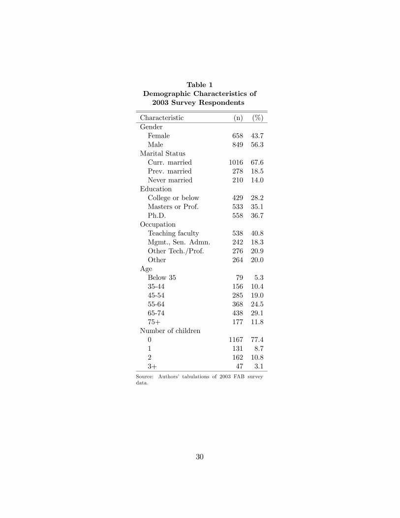
Table 1Demographic Characteristics of2003 Survey Respondents

Characteristic (n) (%)GenderFemale 658 43.7Male 849 56.3

Marital StatusCurr. married 1016 67.6Prev. married 278 18.5Never married 210 14.0

EducationCollege or below 429 28.2Masters or Prof. 533 35.1Ph.D. 558 36.7

OccupationTeaching faculty 538 40.8Mgmt., Sen. Admn. 242 18.3Other Tech./Prof. 276 20.9Other 264 20.0

AgeBelow 35 79 5.335-44 156 10.445-54 285 19.055-64 368 24.565-74 438 29.175+ 177 11.8

Number of children0 1167 77.41 131 8.72 162 10.83+ 47 3.1

Source: Authors’ tabulations of 2003 FAB surveydata.

30

Table 2Ideal and Expected Allocation of

Certificates to First Year

Ideal Expected

Certificates (n) (%) (n) (%)

0 3 0.2 4 0.31 10 0.7 14 0.92 15 1.0 26 1.73 13 0.9 62 4.14 31 2.0 114 7.55 907 59.7 713 46.96 192 12.6 243 16.07 58 3.8 77 5.18 43 2.8 55 3.69 0 0.0 6 0.410 248 16.3 206 13.6Total 1520 100.0 1520 100.0

Source: Authors’ tabulations of 2003 FAB surveydata.

31

Table 3Cross-tabulation of Ideal and ExpectedAllocation of Certificates to First Year

Expected

Ideal 0 1 2 3 4 5 6 7 8 9 10 Total

0 3 0 0 0 0 0 0 0 0 0 0 31 0 10 0 0 0 0 0 0 0 0 0 102 1 0 11 1 1 0 1 0 0 0 0 153 0 0 3 10 0 0 0 0 0 0 0 134 0 0 2 6 20 2 1 0 0 0 0 315 0 1 8 38 76 643 99 28 4 1 9 9076 0 0 0 5 16 40 118 6 6 1 0 1927 0 0 0 1 0 10 9 31 4 0 3 588 0 0 1 0 0 4 8 4 22 1 3 439 0 0 0 0 0 0 0 0 0 0 0 010 0 3 1 1 1 14 7 8 19 3 191 248Total 4 15 28 65 118 718 249 84 63 15 216 1,520

Source: Authors’ tabulations of 2003 FAB survey data.

32

Table 4The Expected-Minus-Ideal Gap

All UncensoredObservations Observations

E-I (n) (%) (n) (%)

5 9 0.6 0 0.04 2 0.1 2 0.23 8 0.5 5 0.42 39 2.6 36 2.91 113 7.4 113 9.00 1,059 69.7 865 69.0-1 141 9.3 138 11.0-2 94 6.2 74 5.9-3 25 1.6 17 1.4-4 9 0.6 2 0.2-5 14 0.9 0 0.0-6 2 0.1 1 0.1-7 1 0.1 0 0.0-8 1 0.1 0 0.0-9 3 0.2 0 0.0Total 1,520 100.0 1,253 0.0

Source: Authors’ tabulations of 2003 FAB sur-vey data.

33

Table 5Net Worth Regression Results

Variable Coeff. Std. Err. Pr > |t|Expected-ideal gap -0.130** 0.055 0.017Ideal level -0.067 0.044 0.127Log 1999 income 0.135 0.170 0.425Zero 1999 income 1.264* 0.728 0.082Past income 0.509*** 0.158 0.001Zero past income 1.467** 0.695 0.035Future income -0.011 0.106 0.916Zero future income -0.037 0.454 0.934Age 0.212*** 0.045 0.000Age2 -0.001*** 0.000 0.003Empl. statusWorking OmittedPartially retired 0.026 0.220 0.906Retired 0.292 0.258 0.258

OccupationFaculty OmittedMgmt./Sen. Admin. -0.156 0.153 0.308Tech./Professional 0.022 0.146 0.881Other -0.099 0.170 0.559

EducationCollege or below -0.305** 0.143 0.033M.A./Profesional OmittedPh.D. -0.032 0.126 0.798

R. has DB plan -0.203 0.126 0.108S. has DB plan -0.080 0.153 0.603Marital statusCurr. married OmittedPrev. married -0.600*** 0.168 0.000Never married -0.344** 0.157 0.029

Male respondent -0.047 0.111 0.673Num. kids 0.028 0.062 0.650Constant -3.046*** 1.117 0.006Source: Authors’ tabulation of 2003 survey data.Notes: The dependent variable is log of net worth. We used a censored regression(Tobit) technique to include people with net worth of zero or less, as well asa multiple imputation process for censored values of the expected-ideal gap; seetext. There were 374 observations used in this regression.

34

Table 6Regressions for Wealth Categories

Non-Retirement Assets Retirement AssetsVariable Coeff. S.E. Pr > |t| Coeff. S.E. Pr > |t|Expected-ideal gap -0.208** 0.087 0.017 -0.079 0.062 0.197Ideal level -0.075 0.076 0.329 -0.014 0.054 0.791Log 1999 income 0.025 0.309 0.935 0.077 0.216 0.720Zero 1999 income 1.069 1.623 0.510 1.387 1.134 0.221Past income 0.867*** 0.303 0.004 0.546*** 0.212 0.010Zero past income 3.495** 1.766 0.048 1.340 1.232 0.277Future income -0.024 0.184 0.894 -0.049 0.128 0.704Zero future income 0.373 0.807 0.644 -0.106 0.563 0.851Age -0.106 0.101 0.294 0.283*** 0.071 0.000Age2 0.001 0.001 0.199 -0.002*** 0.001 0.004Empl. statusWorking Omitted OmittedPartially retired -0.268 0.387 0.489 0.424 0.270 0.116Retired -0.334 0.515 0.516 -0.044 0.360 0.903

OccupationFaculty Omitted OmittedMgmt./Sen. Admin. 0.134 0.262 0.610 -0.087 0.183 0.634Tech./Professional 0.010 0.254 0.968 0.068 0.178 0.701Other -0.003 0.304 0.992 -0.306 0.212 0.149

EducationCollege or below -0.500** 0.249 0.044 -0.368** 0.173 0.034M.A./Profesional Omitted OmittedPh.D. 0.356 0.222 0.108 -0.095 0.155 0.537

R. has DB plan 0.002 0.224 0.994 -0.260* 0.157 0.098S. has DB plan 0.129 0.272 0.635 -0.025 0.190 0.894Marital statusCurr. married Omitted OmittedPrev. married -0.204 0.294 0.487 -0.541*** 0.205 0.008Never married -0.482* 0.278 0.083 -0.337* 0.194 0.083

Male respondent -0.126 0.192 0.510 0.208 0.134 0.121Num. kids -0.065 0.107 0.543 0.004 0.074 0.962Constant 2.208 2.278 0.332 -5.381*** 1.593 0.001

N 362 362

Source: Authors’ calculations based on 2000, 2001, and & 2003 survey data.Note: Dependent variables are natural logarithms of the quantities listed at head of each setof columns. Asterisks indicate the level of statistical confidence for rejection of the hypothesisthat the relevant coefficient is (independently) equal to zero: “***” indicates rejection atbetter than a 1% level of confidence, “**” indicates rejection at better than a 5% level, and“*” indicates rejection at better than a 10% level.

35

Table7The Revealed Preference Gap

RP Gap (n) (%)

10 1 0.15 16 1.24 5 0.43 14 1.12 17 1.31 44 3.30 1,173 88.3-1 32 2.4-2 19 1.4-3 3 0.2-4 3 0.2-5 1 0.1Total 1,328 100.0

Source: Authors’ tabulations of 2003FAB survey data.

36

Table 8Probit Regression for Non-Zero EI Gap

Variable Coeff. Std. err. Pr> |t|Age -0.016*** 0.003 0.000Male -0.166** 0.764 0.030Not Dependable 0.075*** 0.035 0.032Not Organized 0.154*** 0.035 0.000Ideal -0.310*** 0.32 0.000Constant 1.657*** 0.262 0.000

Source: Authors’ tabulations of 2003 Survey Data

37