measuring risk for venture capital and private equity...

1

Measuring Risk for Venture Capital and Private Equity Portfolios

Susan E. Woodward Sand Hill Econometrics

August, 2009

For alternative assets such as venture capital, buyouts (private equity), real estate, etc., the standard regression of portfolio returns on market returns to measure risk produces risk measures that are not credible. Institutional investors, doubting such measures, instead often use either some rule of thumb, such as a stock market index plus a premium (S&P500 + 5, or Russell3000 + 3) as a benchmark, or attempt to evaluate portfolios using public market equivalents. This paper shows an alternative approach to measuring risk directly which explicitly addresses the staleness of reported values for venture capital (and other alternative assets) by including lagging market returns in the regression to capture the full relatedness of portfolio returns to market returns. Examples for venture capital and buyout portfolios show that the true risk measures are generally more than double those from naïve measures lacking lagging market returns. The measurement also reveals the staleness profile of each portfolio, which can be used to calculate a mark-to-market value for the portfolio.

2

Measuring risk for Venture Capital and Buyout Portfolios

Investments in both venture capital and buyouts (also known as “private equity” a

term also used sometimes to include venture capital) are organized as limited partnerships, with a general partner who invests, selects, and manages the assets, and limited partners who merely invest. These investment funds are carve-outs from the 1940 Investment Company Act. As carve-outs of the Forty Act, they are not mutual funds, and are not required to mark-to-market, or to report to any particular convention such as GAAP or SEC rules, to hold liquid assets, or to redeem on any schedule. Reporting of results, in particular, is a matter of contract between the investors and the general partner.1 These limited partnerships cannot take money from ordinary folks, but only from qualified individual investors (rich people, those with net assets of more than $1 million, about 6 million households out of 110 million) and institutional investors. The number of investors may also be limited depending on the minimum wealth levels of the individual investors.

Nearly all limited partnerships investing in venture capital and buyouts (as well as

distressed debt, real estate, oil and gas, essentially all alternatives other than hedge funds) report value to investors on a quarterly basis. The assets in the portfolio are not traded in any public market, and determining their value is not easy. Venture-funded companies are valued every year or two as a result of negotiating price for new rounds of funding. The new price is then carried until there is new event (another round, an IPO, an acquisition, or a shut down) updating the value. As a result, in most quarters, the general partner will not be reporting values that are all current, but instead are a mix of recent and not-so-recent company valuations. For buyouts, there are often no transactions between the time a company is bought into a portfolio and when it is sold. For these, general partners attempt to value the companies through an appraisal process, sometimes quarterly, sometimes less often. Even when performed quarterly, the appraisal process also introduces staleness into valuations. Because the reported values are a mix of current and not-so-current (stale) values, determining the relationship of returns on these assets to returns on a public market portfolio is not so straightforward as for traded portfolios, such as mutual funds, for which a regression of fund returns on market returns reveals most of what a portfolio manager needs to know.

Previous Approaches to Measuring Risk and Performance for Alternative Assets

Many institutional investors do not attempt to measure risk, but implicitly make assumptions about risk by using public benchmarks plus a premium, for example, the S&P500 + 5 of the Russell2000 + 3, and then compare their returns to these benchmarks. Others use the approach of “public market equivalent”, essentially assuming that their portfolios have risk that is the same as that of the stock market. See Long and Nickels

1 Increasingly, many of the investors in such funds are being required to report their portfolio holdings at market values, which is a challenge given the illiquid and untraded nature of the assets.

3

(1995). This approach constructs a portfolio which invests cash and withdraws cash from a stock market index to match the cash flows into and out of venture or buyout investments, and compares the outcomes.

Others who have tried to measure risk acknowledge that stale values in reporting are a problem. Gompers and Lerner (1997) used the return on Nasdaq industry-specific indices from the asset’s last valuation date to the present to bring stale values of individual companies current in venture portfolios, then did the standard regressions. This approach would get us closer to a true risk measure, but only so far as the risk of the companies being marked-to-market is similar to that of the indices used to mark them. The Sand Hill Index for later-stage venture companies, when regressed appropriately on market returns, always yields a beta that is lower than the Sand Hill Index constructed using all (including early stage) venture-funded companies, both for the entire index and for industry subsets. Younger companies are simply more risky, both in terms of the standard deviation of returns and beta. Thus, it unlikely that Nasdaq proxies will mark them to market in an accurate way.

Kerins, Kilholm-Smith, and Smith (2003) substitute returns on newly-public

companies in similar industries to stand in for returns on venture-funded companies. Again, they performed the standard regressions to get measures of systematic and total risk, and again, the proxy is only as good as the risk of the proxy is similar. Newly public companies are more mature than late-stage venture companies, which are more mature than early-stage companies, and risk is commensurate with maturity. Thus, actual venture-funded companies are likely more risky than newly-public companies, and risk measures obtained from newly-public companies are too low for measuring the venture cost of capital.

Emery (2003) uses the standard regression on actual portfolio returns, but uses

returns over longer periods (year vs. quarter) to overcome stale pricing problems. Given that many companies remain at the same value for more than a year, this approach only gets part of the distance to a better risk measure. Even using weekly or monthly returns for public companies, there is still some non-simultaneity of trading, and a Dimson’s adjustment (including one or two lagging and leading market returns in the standard regression) will still capture additional risk that is missed using contemporaneous returns only. The practice of using long time intervals also sacrifices a lot of information that is present in returns over shorter intervals. A measurement that does not require such a sacrifice can be more accurate.

Lundquist and Richardson (2003) also use returns on companies in similar

industry groups to stand in for returns in private equity portfolios to obtain risk measures. Again, the results are as good as the assumption that the stand-ins are good substitutes.

The public market equivalent approach of Long and Nickels, by using the cash

flows into and out of the portfolio, plus public market returns, to simulate the results an investor would have gotten by making the same investments in the public markets. This approach assumes that the portfolio risk is the same as that of the public market, and thus

4

measures only performance, not risk. If the risk of the public market is not the same as that of the portfolio, then the performance measure will be misleading.

This paper offers a way of measuring risk for alternative asset portfolios directly.

Addressing the Staleness in Reported Values To understand the nature of the stale value reporting in venture and buyout

portfolios, it is illuminating to understand how these portfolios are constructed and what are the sources of information for valuation events. Venture Capital funds invest in start-up private companies. Often a first investment is at the stage where the company has only an idea, no customers, no sales, no revenues, perhaps even no office other than a founder’s garage. Investors hope to see the company develop a product, begin selling it, and go public. Only about 20% of venture-funded companies see this outcome. Roughly half fail worthless. For the 30% in between, perhaps 1/3 (10%) are profitable acquisitions, while the other 2/3 (20%) are disappointing acquisitions in which neither the investors nor the founder makes money.

In venture-type investments, funds make a sequence of investments, usually referred to as “rounds” of funding, and at each buy a security called “convertible preferred” stock. The different investments will usually be called something like Series A, Series B, and so on. The shares sold in each round are different securities, with preferences regarding who recovers first in the case of an outcome that cannot pay everyone. (See Litvak (2009) for an informative discussion of the variation in partnership terms.) Investors in each round generally have anti-dilution rights (right of first refusal to investment of a proportionate share in the next round), registration rights (in case of an IPO), and other protections anticipating additional investments and new shareholders.

For the 20% or so of the companies that go public, plus those that have happy acquisitions, everyone converts and the preferences don’t matter. For the 50% that fail worthless, no one converts and the preferences don’t matter. For the outcomes in between, the preferences are often re-negotiated to elicit help from the founders and cooperation from all investors to complete the acquisition. So while preferences may influence value (D shares are worth more than they otherwise would be because they stand in line ahead of A shares), in practice, because of the frequency of re-negotiation in mediocre outcomes, preferences likely matter less than they might seem in the fine print of the offering memorandum or private placement agreement. General partners, in reporting value to investors, generally value all convertible preferred shares, regardless of round, at the same value, and then carry this value until the company has a new valuation event, either a new round of funding, a public offering, is acquired, or shuts down worthless. In other words, in reporting company value, general partners ignore preferences and report all shares at the same value.

5

When a company does a new round of funding, a venture fund will nearly always report (to its limited partners) the value of both newly-acquired shares (say, the C round) plus any shares in a previous round (A round and B round) at the price paid in the new round (despite preferences that may indicate the two types of shares are not of identical value – in other words, the GPs ignore preferences, and they have good reasons, explained above, for ignoring them). At the time of a new round, the shares in previous rounds are marked up to the value of shares in the most recent round. This has important implications for the time series properties of the returns reported by the fund. From quarter-to-quarter when there are no new funding events for a company, shares are carried at the same value, quarter after quarter. When a company does a new round of funding and the shares in prior rounds are marked up to the new value, the fund will report a return for the quarter showing a higher value for that company and consequently, for its entire portfolio. Each quarter, only those companies doing a new round of funding (or exiting through an IPO, acquisition, or shutdown) will change in value. The return on the partnership for the quarter will thus not just be related to stock market changes for the contemporaneous quarter, but also to past quarters back to the date of the previous valuation event(s). It is through this reporting convention that reported returns are smoothed and appear to be less correlated with current market returns than are the unobservable “true economic” returns.

Buyout funds are very different from venture funds. Buyout funds may invest in

private companies or public ones, but in both cases the companies are usually mature and living on their own revenues. They don’t require additional cash from investors to cover costs in the way that venture companies do. For companies in buyout funds, there is no anticipation of additional rounds of funding, hence the security purchased is usually just simple common stock, not convertible preferred stock. Venture deals are nearly always syndicated (multiple funds invest in each round) while buyout deals seldom are. Venture-funded companies almost never have any debt on their balance sheets other than a few trade credits. Because buyout companies are mature and have positive cash flow, they can often be substantially debt financed.

6

Here is a handy list of useful distinctions between venture and buyouts: Venture Buyouts Stage startup mature Revenues? no yes Positive cash flow? no yes Security convertible preferred common stock Debt? rarely often Syndicated? nearly always seldom Industries infotech, biotech all, including the old old thing Failure rate 50% low single digits

Buyout funds buy companies they think are under-valued. Sometimes they buy them from the stock market, sometimes from founders who built them and are ready to relinquish control, and sometimes they buy groups of companies (tire stores, cable TV stations, auto repair establishments), assemble them, brand them, and re-sell them as a single entity. Other times they re-arrange the company’s balance sheet to make it more valuable (get full tax advantage of debt), then re-sell it. In any case, they do not anticipate multiple investments at newly negotiated prices which might reveal value between purchase and sale. Yet they often operate a company for years (as many as 10) as a private company in the fund. In lieu of intermittent funding events that will reveal value, buyout funds revalue their holdings by appraisal methods. The appraisal process also introduces stale values and the smoothing of returns. But as we shall see, the econometrics of de-smoothing returns will look a bit different.

The buyout universe is roughly $1 trillion in the US, much larger than the venture universe, which is now roughly $300 billion in terms of market capitalization. In Europe, where stock markets are a less important part of financing activity, buyouts are more important than in the US. The most spectacular returns are in venture, so it gets attention (mindshare) that is out of proportion to its size.

Measuring Risk: Venture Capital

As a first example to demonstrate how to measure risk when stale values are present, I will use quarterly return data from Cambridge Associates, an institution that advises institutional investors on their “alternative investment” holdings (including venture capital, buyouts, real estate, oil & gas, commodities, and more). These data are posted on the website of CA, and represent the quarterly returns for a large group of venture funds. CA does not reveal whether the series is value-weighted or not. They make no representation regarding the fraction of the universe of possible investments included in these return series. As CA obtains new data, it revises the historical quarterly return series. Over the last few years, the CA quarterly venture returns have been adjusting downwards, while the buyout series has been revised upwards. Compared to

7

returns on average investor portfolios, and to returns on the Sand Hill Index, the average returns in this series are high. They may be biased upwards because investors do not bother to ask consultants for their views on the worst-performing funds. Nonetheless, these return series are informative about risk and useful for illustrating how to measure risk. The estimated alphas thus should not be regarded as a reliable measure of overall venture performance.

First, consider the standard (naïve) CAPM regression of CA venture returns minus the three-month bill rate on the Wilshire5000 minus the three-month bill rate (denoted W below). Here’s the Ordinary Least Squares output:

Table 1: The naïve output for venture capital

Dependent Variable: CAVEN-BILL3MO Method: Least Squares Date: 03/02/09 Time: 13:21 Sample (adjusted): 1989Q1 2008Q3 Included observations: 79 after adjustments

Variable Coefficient Std. Error t-Statistic Prob.

alpha 0.023853 0.012840 1.857746 0.0670W 0.768200 0.162948 4.714385 0.0000

R-squared 0.223989 Mean dependent var 0.036397Adjusted R-squared 0.213911 S.D. dependent var 0.125921S.E. of regression 0.111644 Akaike info criterion -1.522012Sum squared resid 0.959758 Schwarz criterion -1.462026Log likelihood 62.11946 F-statistic 22.22543Durbin-Watson stat 0.758328 Prob(F-statistic) 0.000011

W is the return on the Wilshire5000 (now known as the DowJones Total Stock Market Index) less the return on a 3-month Treasury Bill for the same quarter.

Note the data cover the period 1989q1 to 2008q3, 79 quarters of data. The intercept, alpha, looks impressive: 2.39 percent per quarter, almost double its standard error, for a t-statistic of 1.86. That t-statistic may not reach conventional levels of “confidence” or “significance” but since we financial economists see significant alphas so seldom, it looks pretty good. But the Durbin-Watson (in bold at the bottom left) is only .76. A DW statistic in this range indicates that the residuals in the regression are serially correlated. In regressions like these with stock market data, the DW is always close to 2, indicating no serial correlation in the residuals.

The problem is that individual quarterly returns to venture capital are, by construction, related to not only contemporaneous market returns but also lagging market

8

returns. The method for constructing returns smoothes return and introduces serial correlation into return. The next specification includes lagging market returns (less 3-month bill returns) for five lagging quarters.

Table 2: Measuring risk for venture capital using both current and lagging market returns Dependent Variable: CAVEN-BILL3MO Method: Least Squares Date: 03/02/09 Time: 13:23 Sample (adjusted): 1990Q2 2008Q3 Included observations: 74 after adjustments


alpha 0.001067 0.014350 0.074384 0.9409W 0.788131 0.163942 4.807383 0.0000

W(-1) 0.256860 0.161127 1.594149 0.1156W(-2) 0.317452 0.162761 1.950415 0.0553W(-3) 0.324016 0.164739 1.966852 0.0533W(-4) 0.349472 0.163941 2.131693 0.0367W(-5) 0.166153 0.166482 0.998021 0.3219


Sure enough. Those lagging returns on the public market are indeed related to the quarterly venture returns. Having run thousands of similar regressions on portfolio data, I am confident that the lags go back 5 to 6 quarters. (The lag structure is not stable – in rising markets, fundraising rounds are closer together and the lag structure shortens. In falling markets, they do rounds farther apart, lengthening it. Is this so they can print up-trades sooner, and delay printing down-trades, hoping something good will happen and intervene? Good research question.) Note we lost five quarters of data by introducing lags. If the data have a lag structure, there are inherently fewer observations.

To get the right beta, you simply add up the individual betas, just as you would for a Dimson’s adjustment (or a Scholes-Williams adjustment, depending on where you went to school). In fact, you can think of this specification as an industrial-strength Dimson’s adjustment. (That is how I happened upon it.) Here the sum is 2.22! The difference in beta is large, more than double.

9

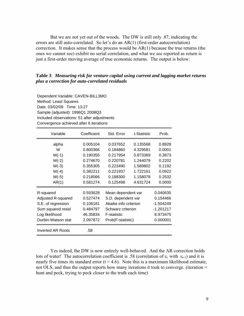
But we are not yet out of the woods. The DW is still only .87, indicating the

errors are still auto-correlated. So let’s do an AR(1) (first-order autocorrelation) correction. It makes sense that the process would be AR(1) because the true returns (the ones we cannot see) exhibit no serial correlation, and what we see reported as return is just a first-order moving average of true economic returns. The output is below:

Table 3: Measuring risk for venture capital using current and lagging market returns plus a correction for auto-correlated residuals Dependent Variable: CAVEN-BILL3MO Method: Least Squares Date: 03/02/09 Time: 13:27 Sample (adjusted): 1996Q1 2008Q3 Included observations: 51 after adjustments Convergence achieved after 6 iterations


alpha 0.005104 0.037652 0.135568 0.8928W 0.800366 0.184860 4.329581 0.0001

W(-1) 0.190355 0.217954 0.873369 0.3873W(-2) 0.274670 0.220781 1.244079 0.2202W(-3) 0.355305 0.223490 1.589802 0.1192W(-4) 0.382211 0.221937 1.722161 0.0922W(-5) 0.218066 0.188300 1.158078 0.2532AR(1) 0.581274 0.125498 4.631724 0.0000


Inverted AR Roots .58

Yes indeed, the DW is now entirely well-behaved. And the AR correction holds lots of water! The autocorrelation coefficient is .58 (correlation of εt with εt-1) and it is nearly five times its standard error (t = 4.6). Note this is a maximum likelihood estimate, not OLS, and thus the output reports how many iterations it took to converge. (iteration = hunt and peck, trying to peck closer to the truth each time)

10

The total beta is 2.22, close to what we got without the AR correction. Without the AR correction, OLS is still unbiased, but it is not minimum variance. The AR correction gives us an estimate that is minimum variance as well as unbiased. The correction might move the beta up or down (usually +/- 10 to 15% in my experience), but it is nearly always a better fit, in the sense that the standard error on beta is smaller. The difference between using lags vs. not using lags is enormous, and gets much closer to a true measure of risk. In comparison, the AR correction is a frill. But it is a cheap frill, so let’s keep it.

There is one more frill. Surely you are terribly curious about the standard error on the total beta – the sum of the individual betas, to indicate how “good” is the measure of beta. With the right set-up, you can make any standard program compute that standard error for you. If W is the coefficient on your contemporaneous return (less the 3-month bill rate), subtract it from all the other regressors. See the output below: Table 4: Measurement of risk for venture capital using a specification which will generate standard errors for the total portfolio beta Dependent Variable: CAVEN-BILL3MO Method: Least Squares Date: 03/02/09 Time: 13:30 Sample (adjusted): 1996Q1 2008Q3 Included observations: 51 after adjustments Convergence achieved after 6 iterations


alpha 0.005104 0.037652 0.135568 0.8928W 2.220972 0.778689 2.852195 0.0066

W(-1)-W 0.190355 0.217954 0.873369 0.3873W(-2)-W 0.274670 0.220781 1.244079 0.2202W(-3)-W 0.355305 0.223490 1.589802 0.1192W(-4)-W 0.382211 0.221937 1.722161 0.0922W(-5)-W 0.218066 0.188300 1.158078 0.2532

AR(1) 0.581274 0.125498 4.631724 0.0000



11

Note that the coefficient on W is 2.22, and it is exactly the sum of the betas in the previous specification. All other coefficients are the same and have the same standard errors and t-statistics as before. All other summary statistics are the same – same r-sq, same DW, same F. What is special about this setup is that you can read directly the beta and its standard error as reported in the standard output. The total beta is nearly three times its standard error, so we can declare it to be well-measured. Not quite like stock market data, but hey, so many people have claimed it was impossible to measure risk for these limited partnerships that I have declared victory.

So this is it – this is your answer. Using the data from 1989 to the present, the beta for venture capital is 2.2, more than double the beta of the stock market. The residual variance is large also. This output reports the residual variance of the smoothed returns, not the true economic returns. Ditto for the r-square (and its square root). If you want a residual variance and correlation with the market for true venture returns (instead of smoothed ones), use the equations below, which appear in Woodward (2005).

σtrue = σsmoothed (1/Σ w2i) ½ where wi = βi/Σ βi (1)

Think of w as the weight or proportion of beta (β) coming from each of the market

returns used in the regression. You could also use

σ2true = (Σ βi) 2 (σ2

m ) + (σ2η )(1/Σ w2

i) (2) where σ2

m is the variance of the market portfolio and σ2η is the residual variance of the

smoothed portfolio returns as reported in the regression output. Equation (2) just decomposes the total variance given in (1) into the systematic and residual variance.

And for the correlation with the market:

ρtrue = ρsmoothed (w0 (1/Σ w2i)) (3)

where ρsmoothed is the square root of the r-square reported in the regression (not using the AR correction) and w0 is the proportion of beta coming from the contemporaneous market return, or the weight for the contemporaneous return. Derivations are in Geltner (1991).

One more interesting fact before we leave venture capital. The beta for venture has fallen dramatically since the dotcom bust. The next measurement uses data from just the period from 2002q2 to 2008q3:

12

Table 5: Measurement of risk for venture capital in the post-dotcom era: Dependent Variable: CAVEN-BILL3MO Method: Least Squares Date: 02/03/09 Time: 13:41 Sample (adjusted): 2002Q1 2008Q3 Included observations: 27 after adjustments Convergence achieved after 9 iterations


alpha -0.006553 0.009858 -0.664761 0.5142W 1.083701 0.264174 4.102217 0.0006

W(-1)-W 0.107879 0.075463 1.429568 0.1691W(-2)-W 0.125762 0.072750 1.728684 0.1001W(-3)-W 0.146957 0.076355 1.924659 0.0694W(-4)-W 0.079816 0.078422 1.017783 0.3216W(-5)-W 0.218281 0.067973 3.211281 0.0046

AR(1) 0.446559 0.188822 2.364974 0.0288

R-squared 0.792706 Mean dependent var -0.001847Adjusted R-squared 0.716335 S.D. dependent var 0.049543S.E. of regression 0.026387 Akaike info criterion -4.190708Sum squared resid 0.013229 Schwarz criterion -3.806756Log likelihood 64.57455 F-statistic 10.37961Durbin-Watson stat 2.257091 Prob(F-statistic) 0.000024


The beta is now down at about 1.1, vs. the 2.2 for the entire period. Despite the negative alpha, this alpha is still higher than what we see in customer data or from the Sand Hill Index. The 2000 vintage year for venture capital (the set of companies doing their first round of funding in 2000) is not going to return capital to investors, and it was a year of very large amounts invested (more than $95 bn was invested into venture-funded companies, vs $25-30 bn per year for the years since 2002). I believe this will be the first cohort of venture-funded companies that will fail, overall, to return capital.

We regularly look at four sets of returns on venture capital. One set is the CA returns you see here. Another is returns from Thomson VentureEconomics. The Thomson figures are proprietary (not disclosed on a public web site) and not presented here, but they are only a little different. Consistently venture betas calculated using CA data are higher than those from Thomson data. But both CA and Thomson data are biased upward compared to customer returns we see or to the Sand Hill Index. From Sand Hill data we get a beta that lies between the CA and Thomson betas, but a lower alpha than

13

for either. The fourth set of data we look at is from customers (actual investor results) at of large asset custodian. Their betas are also in between, and their alphas are on average about zero.

It is at the portfolio level that this method succeeds best in measuring risk. It is

not a useful approach for analyzing returns on individual partnerships. Individual partnerships begin with new investments in young companies, and these companies mature as additional investments are made. The risk in the portfolio changes as the companies mature. At the portfolio level, there is usually a mix of partnerships, some young, some older, some in-between at all points in time.

Not only do risk levels change through the life of a given fund, performance

changes also. The high returns nearly always occur early in the life of a portfolio, seemingly simply because the most valuable investments become obviously valuable soon. Thus, early exits are better than average, while later exits are the poorer outcomes. The CA data used here appear to represent a mix of funds of different ages in every quarter, as we would see in the typical investor’s mature venture portfolio. It is not unusual for an institutional investor in venture capital to have 30 to 50 different partnerships, containing 1,200 or 1,500 unique portfolio companies. If a portfolio is comprised of entirely young partnerships, or entirely older partnerships, this method is likely to work less well, or to require some adjustments of interpretation. Measuring Risk: Buyouts

As I suggested earlier, the private equity or buyout sector is large, close to a trillion dollars in the US. CA makes no claims about what fraction of buyout investments their return data represent. The beta for CA buyouts is a bit higher than the beta for other buyout return series such as Thomson or customer portfolio returns. Perhaps this is because the customers of Cambridge Associates tend to be endowments rather than pension plans, and endowments do take more risk. How they choose their funds to be more risky or less is not clear. Again, here is the standard (naïve) regression for buyouts:

14

Table 6: The naïve measurement of risk for buyouts (private equity) Dependent Variable: CABUY-BILL3MO Method: Least Squares Date: 03/02/09 Time: 13:38 Sample (adjusted): 1990Q1 2008Q3 Included observations: 75 after adjustments


alpha 0.020794 0.004116 5.052616 0.0000W 0.418697 0.051622 8.110801 0.0000


Looks great, no? A money printing machine. The beta is only .4 and the alpha is 2 percent per quarter. Well, … maybe not. Look again at the DW. Only 1.34, so there is some serial correlation in the errors. Again, we add lagging market returns to the specification. Again, from running thousands of these, I am confident that 5 or 6 lagging quarters will pick up everything that is there. Now add an AR(1) correction and use that specification that calculates the SE on the full beta.

15

Table 7: The measurement of risk for buyouts using current and lagged market returns and correction for auto-correlated residuals Dependent Variable: CABUY-BILL3MO Method: Least Squares Date: 02/03/09 Time: 13:21 Sample (adjusted): 1996Q1 2008Q3 Included observations: 51 after adjustments Convergence achieved after 6 iterations


alpha 0.014102 0.005788 2.436321 0.0191W 0.963550 0.141606 6.804464 0.0000

W(-1)-W 0.180940 0.054331 3.330340 0.0018W(-2)-W 0.116670 0.054763 2.130447 0.0389W(-3)-W 0.054044 0.055451 0.974638 0.3352W(-4)-W 0.067735 0.055352 1.223712 0.2277W(-5)-W 0.058785 0.054154 1.085517 0.2837

AR(1) 0.165040 0.151824 1.087055 0.2831



Using lagging returns and an auto-regressive correction, the beta is .96, more than double the naïve estimate of beta. So the proportional correction to the risk measure by adding lags for buyouts is roughly similar to that for venture capital. The risk measure more than doubles. And as for venture, the corrected alpha is substantially lower. This makes sense, because if beta is biased downwards, the alpha (intercept) will be biased upwards. A downward-biased beta attributes too little return to risk and too much to other stuff, like skill.

Note that the AR correction is not as important for buyouts as for venture. The AR coefficient is smaller, and it is not quite double its standard error. But it does bring the DW into the range where it should be, so all things considered, I always keep it. Plus, when the coefficient is larger than its standard error, the estimated coefficient is a more likely value than is zero. If you don’t have a strong prior, go with the estimate.

16

There’s good economic logic for why the AR correction is less profound for buyouts then for venture. The lag structure for buyouts is simply not as “structured” as for venture. For buyouts, the staleness in pricing or smoothing of returns is coming from an appraisal process rather than from simply carrying old values until they are updated with a new funding event or exit. The staleness of appraisals is random – it may be that the general partner is comparing a company to something from 6 months ago, a year ago, or something current. Sometimes it is close, other times not so close. Buyout appraisal values do not have the lock-step auto-regressive properties that venture valuations from funding rounds have.

Again, the standard regression output does not give you the residual variance of the true, economic returns, but of the smoothed, reported returns. To recover true sigma, and true correlation, use equations (1), (2), and (3) above. The sigma of the true economic returns will be more than double the sigma of the (smoothed) reported returns.

As with venture capital, CA buyout returns always give higher betas than do Thomson buyout returns, and the customer betas are in between. The CA and Thomson alphas are substantial, even after adding lags and AR corrections. In the customer data, the alphas are much closer to zero. Alas, there appears to be no premium for illiquidity. It is not inappropriate to think of buyouts as S&P500 exposure that is liberated from marking-to-market. Do investors value this liberation? Another good research question.

An interesting difference between venture risk and buyout risk is that unlike venture risk, buyout risk has not changed. Here’s an estimate using only post-dotcom boom returns:

17

Table 8: Measurement of risk for buyouts in the post-dotcom era

Dependent Variable: CABUY-BILL3MO Method: Least Squares Date: 03/02/09 Time: 13:57 Sample (adjusted): 2001Q3 2008Q3 Included observations: 29 after adjustments Convergence achieved after 7 iterations


alpha 0.021380 0.005194 4.116153 0.0005W 1.058180 0.152106 6.956877 0.0000

W(-1)-W 0.133239 0.075023 1.775978 0.0902W(-2)-W 0.145247 0.073215 1.983833 0.0605W(-3)-W 0.109673 0.071888 1.525600 0.1420W(-4)-W 0.127129 0.070011 1.815840 0.0837W(-5)-W 0.070729 0.070337 1.005563 0.3261

AR(1) -0.097931 0.232021 -0.422080 0.6773


Inverted AR Roots -.10

Whatever they were doing before, they are doing more of it. Telecom, yes, but

also pie shops, tires, pizza, tv stations, specialized metal fabrication, and not much start-up software or pharma.

One more question: do we need to run the regression separately for up markets and down, as is often done for hedge funds, to test for asymmetric exposure, or poke around for out-of-the-money puts and what not? The answer is no. These portfolios have a great deal of inertia, there is essentially no trading in them, and their exposure is symmetric. Marking-to-Market

As the pressure to report all portfolio values at current market value rises, one instinct is to try to obtain a current value for every quarter for every company in the portfolio. The portfolio-based approach here has a substantial advantage over the

18

company valuation approach. The portfolio approach does not require estimation of individual company values. Instead it merely exploits the underlying systematic relationship between changes in reported values and current and lagging market returns. For venture capital, no estimated values are used in the portfolio approach. The relationship between market returns and venture returns is measured acknowledging the presence of stale values, and incorporating lagging market returns to adjust for them.

The pattern of staleness is revealed in the fraction of the total beta that comes

from the different coefficients. The coefficient weights, the wi in equations (1), (2), and (3), reveal how much of beta is coming from the contemporaneous return, a return one quarter lagging, two quarters lagging, and so on. Thus, if the weight on the current return is 50%, we know the portfolio value is 50% current. If the sum of the coefficients, the total beta is βtotal, and the coefficient on the current market return is β0, then the proportion of the portfolio whose value is current is β0 / βtotal = w0. The proportion that is one-quarter stale is β-1 / βtotal = w1. If the weight on the return lagging one quarter is 19%, then we know that 19% of the value is one quarter old. To mark the portfolio to market, multiply the fraction of the portfolio that is n quarters old by the market return since that period times the beta for the portfolio.

Table 9: Coefficients and weights for portfolio measurements in Table 7

variable coefficient value Weight W 0.49 0.50

W(-1) 0.18 0.19 W(-2) 0.12 0.12 W(-3) 0.05 0.06 W(-4) 0.07 0.07 W(-5) 0.06 0.06

total beta: .96

w0 = β0 / βtotal = .49/.96 = .50, and w1 = β-1 / βtotal = .18/.96, and so on, in the above example. Generally, the mark-to-market value implied by the estimated coefficients is given by

current value = (reported value) * βtotal * [w0 + w1 (1+Rm,-1) +

w2 (1+Rm,-1) (1+Rm,-2) +

· · · + wn (1+Rm,-1) · · · (1+Rm,-n) ]

19

where Rm,-1 is the return on the market portfolio over the past quarter, and so on. The market return measure used in the regressions here is the Wilshire5000. We use it in preference to other market measures because it picks up more relationship between venture-funded companies and the stock market than do other broad indices, likely because it includes many more tiny companies than do other equity market indexes. Marking-to-market via this portfolio approach is both easier and more straightforward than trying to mark each company value to market separately. Especially given the difficulty of valuing the youngest companies, which lack revenue and customers, taking advantage of the systematic relationship between portfolio values and current and lagging market values may make more sense, and be more accurate, than trying to mark each company individually. The accounting rules that call for marking-to-market are not those governing the relationship between the general and limited partners, but instead the requirements that pension plans sponsored by public companies, some endowments, and all public companies must report the value of their assets to their investors at market values. SFAS (2007) defines fair value as the “price that would be received to sell an asset of paid to transfer a liability in an orderly transaction between market participants at the measurement date”. Because these partnership interests change hands very seldom, there are no market prices upon which the reporting entity may rely. Acknowledging that such situations would arise, SFAS 157 created a hierarchy of approaches to valuation depending on what is available: Levels 1: prices observed in the market (e.g., identical or close-to-identical traded securities); Level 2: prices based upon inputs observed in the market (e.g., price changes in similarly-rated bonds of the same maturity); and Level 3: prices based on unobservable inputs (such as volatility parameters used in valuing options that much be calculated from other market data). These are sometimes referred to as “mark-to-market, mark-to-matrix, and mark-to-model”. The approach here falls into the “mark-to-model” category, because the staleness profiles are not evident to the naked eye, but must be recovered from regressions of portfolio returns on market returns. The approach begins with actual prices, some of which are known to be stale. The model (the regression of fund returns on market returns) coefficients that provide us with a beta also reveal the fraction of reported value that is stale by 1 quarter, 2 quarters, and so on. These staleness parameters and the beta are not “observable” to the naked eye, but the regression of fund or portfolio returns on current and lagging market returns reveals them. The staleness profile revealed in the coefficients can used to calculate estimated current values. The advantages of this approach over valuing individual companies are considerable. First, the validity and integrity of the relationship between reported values (which are partly stale) and market returns is stable, verifiable, and systematic. Second, the model not only produces an estimate of current value, it also produces standard errors for the estimate. While individual company valuations based on methods such as discounted-cash-flow are often plausible and reasonable, they never come with statistically reproducible standard errors to provide a measure of how much error might be present.

20

Third, this approach is very inexpensive compared to re-valuing each and every company. In sum, measuring risk for portfolios of illiquid assets is eminently feasible. It is only a bit more complicated than measuring risk for a traded portfolio, though it cannot be done with most canned software used to measure risk for traded portfolios. The approach that gets the risk measure right produces risk measures that are typically more than double the result from a naïve measurement. The improved approach not only produces a more realistic measure of risk, it also reveals the staleness profile of the portfolio, which then allows for a straight-forward marking of the portfolio to market.

21

References:

Asness, Clifford, Robert Krail, and John Liew, (2001) “Do Hedge Funds Hedge?” Journal of Portfolio Management, Fall

Dimson, Elroy, (1979) “Risk Measurement when Shares are Subject to Infrequent Trading” Journal of Financial Economics, 7

Emery, Kenneth, (2003) “Private Equity Risk and Reward: Assessing the Stale Pricing Problem” Journal of Private Equity, Spring

Financial Accounting Standards Board (2007, February), “The fair value option for financial assets and financial liabilities”, including an amendment of FASB No. 115. Norwalk, Connecticut.

Getmansky, Mila, Andrew Lo, and Igor Makarov, (2005) “An Econometric Model of Serial Correlation and Illiquidity in Hedge Fund Returns”, Journal of Financial Economics

Geltner, David M. (1991) “Smoothing In Appraisal-Based Returns” Journal of Real Estate Finance and Economics, September

Gompers, Paul, and Josh Lerner (1997), “Risk and Reward of Private Equity Investments: The Challenge of Performance Assessment”, The Journal of Private Equity, Vol.1, No.2, Winter.

Hall, Robert, and Susan E. Woodward, (2009), “The Burden of the non-diversifiable risk of Entrepreneurship”, American Economic Review, forthcoming.

Litvak, Kate, (2009) “Venture Capital Partnership Agreements: Understanding Compensation Arrangements, University of Chicago Law Review, forthcoming.

Long, Austin M., and Craig Nickels, (1995) “A Method for Comparing Private Market Internal Rates of Return to Public Market Index Returns” manuscript, University of Texas Retirement System, August 28.

Lundqvist, Alexander, and Matthew Richardson, (2003) “The Cash Flow, Return, and Risk Characteristics of Private Equity” NBER Working paper #9495, January.

Kerins, Frank, Janet Kiholm Smith, and Richard Smith, (2003) “Opportunity Cost of Capital for Venture Capital Investors and Entrepreneurs” working paper, February.

Scholes, M., and J.T. Williams, (1979) “Estimating Betas from Non-Synchronous Data, Journal of Financial Economics, 5

Woodward, Susan E. (2005) “Measuring and Managing Alternative Assets Risk”, Global Association of Risk Professionals, May

Woodward, Susan E., and Robert E. Hall, (2003) “Benchmarking the Returns to Venture” NBER Working Paper 10202, December.

measuring risk for venture capital and private equity...

Documents