measuring prevalence, profiling and evaluating the...
TRANSCRIPT
1
Measuring Prevalence, Profiling and Evaluating the Potential of Policy Impacts using Two
Food Security Indicators in Guatemala
Luis Sandoval*
Graduate Student
Carlos E. Carpio*
Associate Professor
*Department of Agricultural and Applied Economics
Texas Tech University
Selected Paper prepared for presentation at the Southern Agricultural Economics Association’s
2017 Annual Meeting, Mobile, Alabama, February 4-7, 2017.
Copyright 2017 by Sandoval and Carpio. All rights reserved. Readers may make verbatim copies
of this document for non-commercial purposes by any means, provided that this copyright notice
appears on all such copies.
2
Measuring Prevalence, Profiling and Evaluating the Potential of Policy Impacts using Two
Food Security Indicators in Guatemala
Luis Sandoval and Carlos Carpio
Introduction
The concept of food security1 can be applied and used to analyze individuals, households,
nations or even the entire globe. In particular, a household is said to achieve food security when
all its members have access to the food they need for an active and healthy life (FAO, 1996), and
thus, food security at this level is usually measured in the access dimension2 of the food security
concept. Prominent examples of indicators developed for this purpose are the Latin American
and Caribbean Food Security Scale (ELCSA) and the household level IFPRI’s undernourishment
indicator. Although the two indicators are calculated differently, both use information collected
at the household level and can also be used to estimate the prevalence of food insecurity in a
region or country, making them suitable for national level policy analyses (FAO, 2012; Smith
and Subandoro, 2007).
ELCSA is an experiential measure obtained by asking households a series of questions
aimed to evaluate their food security concerns and experience. Modeled after the United States
Department of Agriculture’s (USDA) Household Food Security Survey Module, this food
security indicator has been adapted and validated for use in Latin America and the Caribbean
1 Food security exists when all people, at all time, have physical and economic access to sufficient, safe and
nutritious food to meet their dietary needs and food preferences for an active and healthy life (FAO, 1996). 2 Four dimensions can be identified from the food security concept: availability, economic and physical access,
utilization and stability.

3
(FAO, 2012). On the other hand, IFPRI’s undernourishment indicator is constructed using
Household Expenditure Surveys (HES) data (Smith and Subandoro, 2007).
Because indicators such as ELCSA and IFPRI’s undernourishment indicator operate in
the same dimension of food security (access), at the same level (household level), and provide
the same output (food security status of the household), they tend to be used interchangeably,
which may result in the misclassification of households as food secure or insecure with further
implications regarding their inclusion or exclusion from assistance programs (Maxwell et al.,
2014). For example, as shown in this paper, the use of these two indicators can result in different
estimates of the prevalence of food insecurity in a region or country, which in turn can lead to
substantially different policy recommendations or courses of action aimed to address food
security problems. Therefore, the objectives of this paper are: 1) to measure and compare the
prevalence of food insecurity in a country using the alternative ELCSA and IFPRI’s
undernourishment indicator, 2) to identify the factors affecting households’ food security status
using the two indicators, and 3) to assess the use of the two indicators for policy analysis.
Data for the study comes from the 2011 National Survey of Living Standards (ENCOVI)
from Guatemala, which collects the necessary information to estimate both indicators for the
same households. We focus on these two indicators given their growing importance to assess the
status of food security. ELCSA is gaining popularity in Latin America and the Caribbean and is
now included as part of the nationally representative HES in several countries. IFPRI’s
undernourishment is also being used more frequently as more countries are periodically
conducting national representative HES. Even though several studies have compared food
security indicators, their focus has been in the estimation of the prevalence of food insecurity

4
without attention to the implications of their use for policy analysis (Maxwell et al., 2014; Leroy
et al., 2015; Haen et al., 2011).
The Latin America and Caribbean Food Security Scale (ELCSA)
The ELCSA is a survey based food security Experiential Measure that operates on the
access dimension of the food security concept. The indicator evaluates how households’
experience food security by assessing their concerns and experiences, during the last three
months prior to the interview, with respect to the quantity and quality of their diet and their use
of coping strategies, such as eating less than usual or skipping meals.
Several reasons make the ELCSA an attractive food security indicator. First, the ELCSA
is a direct measure of household food security significantly less expensive to implement than
food security measurements based on food consumption and expenditure surveys. Second, since
it is a standardized measure it can be used for cross country comparisons (FAO, 2012). Finally,
ELCSA does not only classify households as food secure and insecure but also provides different
levels of food insecurity (see Table 1). ELCSA has been validated in several Latin American
countries and is currently included in national surveys in Brazil, Bolivia, Colombia, El Salvador,
Guatemala and Mexico (FAO, 2012).
ELCSA consists of a set of 15 questions. The answer to each of the questions are simple
‘yes’ or ‘no’ and the food security status of the household is then estimated depending on the
number of affirmative answers to the questionnaire. When households have no children only the
first eight questions are asked, since the following seven question are intended to measure the
food security status of children only. There are four possible categories for the food security
status of a household: food secure, mild food insecure, moderate food insecure and severely food

5
insecure (see Table1). Appendix 1 includes the ELCSA questionnaire currently used in
Guatemala.
Table 1. ELCSA's food security categories and required affirmative answers.
Category Households with children Households without children
Food secure 0 0
Mild food insecure 1 – 5 1 – 3
Moderate food insecure 6 – 10 4 – 6
Severe food insecure 11 – 15 7 – 8
Source: Melgar-Quiñonez and Samayoa (2011).
IFPRI’s Undernourishment Indicator
IFPRI’s undernourishment indicator is estimated from HES and compares the caloric
requirements of a households with the calories it has available for consumption from all food
sources to determine if the household is energy deficient (Smith and Subandoro, 2007).
Household consumption and expenditure surveys are part of nationally representative living
standard surveys that are now being periodically conducted in several countries in the world.
These surveys became popular in the 1980’s thanks to efforts such as the Living Standards
Measurement Study of the World Bank, which works with national statistics offices to help them
design multi-topic household surveys (World Bank, 2016). In 2007, researchers at IFPRI
developed a technical guide to measure food security using household expenditure surveys
(Smith and Subandoro, 2007). Their objective was to reduce the gap between more accurate and
costly measurements of undernourishment at the individual and household level that were being

6
carried out in only small populations, such as dietary recall diaries3 and less accurate and
aggregate methods for large populations, such as FAO’s prevalence of undernourishment
indicator. Smith and Subandoro (2007) show how the information from HES can be used to
define several household level food security indicators including a household level
undernourishment indicator, which we refer to as IFPRI’s undernourishment indicator4. The
other indicators proposed by these researchers were: an indicator of diet diversity, percentage of
dietary energy in the household derived from staples, quantities of individual food consumed per
capita, and percentage of household expenditures devoted to food. In this paper, we focus only
on IFPRI’s household level undernourishment indicator since all other indicators do not provide
cutoff points to classify households as food secure or insecure.
Literature Review
Most of the literature comparing food security indicators concentrates on discussing the
advantages and disadvantages of the different indicators and little research has been conducted to
evaluate differences on food security assessments when the indicators are implemented
(Maxwell et al., 2014; Maxwell et al., 2013). To the best of our knowledge, no previous study
has compared ELCSA and IFPRI’s undernourishment indicator; however, we did identify one
study that compared an indicator very similar to ELCSA, the Household Food Insecurity Access
Scale (HFIAS), to other food insecurity indicators, and three studies exploring the relationship
3 In dietary recall diaries households recall what they ate, by member of the household, for a given period of time.
Because the required level of detail it’s necessary to train households in its utilization, which increases their
implementation cost. 4 It is important to do not confuse IFPRI’s undernourishment indicator with FAO’s prevalence of undernourishment.
FAO’s indicator relies on FAO’s food balance sheets and measures the probability that a randomly selected
individual would consume less calories than his requirement for an active and healthy life . (FAO, IFAD, and WFP,
2016).

7
between ELCSA and data from household expenditure surveys (Valencia-Valero and Ortiz-
Hernandez, 2014; Carrasco et al., 2010; Vega-Macedo et al., 2014)
Maxwell et al. (2014) compared seven frequently used indicators of food access using
data from a panel survey of rural households in Ethiopia. The study compared an experiential
measure, the HFIAS, which is very similar to ELCSA, to dietary diversity, food frequency,
consumption behaviors and self-assessment indicators but no undernourishment. Their results
showed correlations between 0.46 and 0.85 (absolute values) between the HFIAS and the other
food security indicators with the HFIAS always producing between 15 to 75% higher prevalence
of food insecurity than the other indicators. They concluded that HFIAS tends to give higher
estimates of prevalence of food insecurity because it captures physiological anxiety and
preferences, which are not severe manifestations of food insecurity. Moreover, a single
occurrence of a food insecurity experience can move a household towards a more critical food
insecurity category. Despite the differences in the categorization of food insecure households, all
the indicators exhibited similar trends across time in the incidence of food insecurity. Moreover,
these authors argue that the observed differences in the percentages of households that are
classified as food insecure using different indicators are due to three main reasons. First, the cut-
offs points for the classification of households as food secure or insecure are not harmonized
across indicators; second, different indicators measure different dimensions of food insecurity;
and third, the indicators differ in their sensitivity to the severity of food insecurity.
Data and Methods
Data for our analyses comes from the 2011 National Survey of Living Standards
(ENCOVI) from Guatemala. According to Guatemala’s National Institute of Statistics (INA), the
main objective of the survey was to estimate the incidence of poverty in the country. The survey

8
was conducted between March and August and reached more than 13 thousand households (INE,
2011). The ELCSA questionnaire was collected as part of the dwelling and household chapter of
the survey and food expenditures were collected as part of the expenses and self-consumption
chapter. The food expenditures section collected quantity and monetary value of food purchases
for a 2-week recall period, quantity and monetary value of self-produced food products or
obtained free of charge for the 2-week recall period and weekly expenditures in food eaten away
from home. Age, sex and activity level of the household members, required for estimating the
household’s energy requirements, were also collected as part of the demographic characteristics
and the employment and activities sections.
Nutritional information on the food items found in the HES was obtained from the Table
of Nutritional Composition of Central American Foods by the Central America and Panama
Institution of Nutrition (INCAP, 2012). The table provides information on the content of 28
nutrients for 1,169 food products in the region.
Estimation of the Indicators
The procedures to estimate ELCSA and IFPRI’s undernourishment indicators are
summarized in Figure 1.

9
Figure 1. Summary of procedure used for estimating ELCSA and IFPRI’s undernourishment
indicators.
As it can be seen from Figure 1 the estimation procedure of the food security status of a
household is simpler using the ELCSA method than with IFPRI’s method. In the case of IFPRI’s
undernourishment indicator, we followed the method suggested by Smith and Subandoro (2007).
First, we converted the quantities of foods acquired from all sources to calories (i.e., energy) to
have an estimate of the household available energy. Second, the household caloric requirement
was estimated taking into consideration the sex, age and physical activity of each household
member following FAO’s recommendations and tables (2001). Finally, the household energy
ELCSA
Collect survey data:
ELCSA questionarie
The food security level is estimated depending on the number of affirmative answers to survey questions
A household is clasified as food secure if it responds negatively to all questions
IFPRI's undernourishment indicator
Collect survey data:
1. Food expenditures, food production for self consumption and food obtained free of charge.
2. Age, gender and physical activity level of the household members is collected.
Collect data on nutritional composition of foods and individuals' daily energy requirements
Estimate household foood energy balance by substracting the energy requirement of the household from the energy available from all food sources
A household is classifed as food secure when food energy balnce is zero or positive

10
balance was estimating by subtracting the household’s available energy from its caloric
requirement.
For the purpose of our analysis we focused on the classification of households as either
food secure or food insecure. In the case of ELCSA, households that respond negatively to all
questions in the instrument are classified as food secure (see Table 1). If they respond
affirmatively to at least one of the questions they are classified as food insecure. When using
IFPRI’s undernourishment indicator, households are classified as food secure if they are not
energy deficient (they have more calories available than their daily requirement) and as food
insecure if they are energy deficient.
Logistic Regression
To evaluate the effect of socio-demographic characteristics on household food security
status we estimated logistic regression models using ELCSA and IFPRI’s undernourishment
indicators as dependent variables. For each dependent variable, we estimated two regression
models, one for the entire population and another only for poor households since they are the
focus of our policy simulations. In addition, preliminary data analysis suggested significant
differences in the parameter estimates between models using the entire population and models
for the poor only. The probability of households being food insecure can be expressed as 𝜋 =
Pr(𝑌 = 1|𝒙), where x is a vector explanatory variables (see Table 2). The logistic model has the
following functional form (Greene, 2012):
(1) 𝑙𝑜𝑔 (𝜋
1−𝜋) = 𝛼 + 𝜷′𝒙,
where α and β are parameters to be estimated. All models were estimating by Maximum
Likelihood using the LOGISTIC procedure of the SAS® 9.4 software.

11
Table 2. Explanatory variables for the logistic regression models
Category Variable Description Mean
Standard
Deviation Minimum Maximum
Continuous
variables
Number of household
members
Number of household members. 4.934 2.451 1.000 22.000
Per-capita annual
expenditures
Per-capita annual expenditures in Guatemalan
quetzals (GTQ). 11.797 12.356 0.535 305.999
Dummy
variables
North Indicates if the household is located in the North
region. 0.069 0.254 0.000 1.000
Northeast Indicates if the household is located in the Northeast
region. 0.224 0.417 0.000 1.000
Southeast Indicates if the household is located in the Southeast
region. 0.103 0.304 0.000 1.000
Central Indicates if the household is located in the Central
region. 0.157 0.364 0.000 1.000
Southwest Indicates if the household is located in the
Southwest region. 0.271 0.444 0.000 1.000
Northwest Indic0.031ates if the household is located in the
Northwest region. 0.071 0.256 0.000 1.000
Peten Indicates if the household is located in the Peten
region. 0.031 0.173 0.000 1.000
Female Indicates if the head of the household is female. 0.206 0.405 0.000 1.000
Indigenous Indicates if the head of the household is indigenous. 0.344 0.475 0.000 1.000
Rural Indicates if the household is located in the rural
area. 0.586 0.493 0.000 1.000

12
July-August Indicates if the survey was taken during the last
third of the lean season5. 0.200 0.400 0.000 1.000
Presence of Children Indicates if there are under 18 years old in the
household. 0.792 0.406 0.000 1.000
Primary and middle school
education
Indicates if the head of the household has primary or
middle school education. 0.651 0.477 0.000 1.000
University education Indicates if the head of the household has university
education 0.035 0.183 0.000 1.000
Poverty Indicates if the household is considered poor by the
government. 0.54 0.498 0.000 1.000
5 Lean season is period of the year in which rural and poor households are most food insecure and most likely to require food aid (FAO, IFAD and WFP, 2016)
13
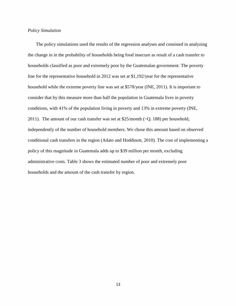
Policy Simulation
The policy simulations used the results of the regression analyses and consisted in analyzing
the change in in the probability of households being food insecure as result of a cash transfer to
households classified as poor and extremely poor by the Guatemalan government. The poverty
line for the representative household in 2012 was set at $1,192/year for the representative
household while the extreme poverty line was set at $578/year (INE, 2011). It is important to
consider that by this measure more than half the population in Guatemala lives in poverty
conditions, with 41% of the population living in poverty and 13% in extreme poverty (INE,
2011). The amount of our cash transfer was set at $25/month (~Q. 188) per household,
independently of the number of household members. We chose this amount based on observed
conditional cash transfers in the region (Adato and Hoddinott, 2010). The cost of implementing a
policy of this magnitude in Guatemala adds up to $39 million per month, excluding
administrative costs. Table 3 shows the estimated number of poor and extremely poor
households and the amount of the cash transfer by region.

14
Table 3. Average monthly benefits of the cash transfer policy simulation.
Percentage of poor and
extremely poor
households
Number of poor and
extremely poor
households
Value of the cash
transfer
Metropolitan 36% 270,192 $6,754,801
North 66% 176,057 $4,401,435
Northeast 48% 126,203 $3,155,082
Southeast 53% 127,555 $3,188,874
Central 54% 188,284 $4,707,107
Southwest 61% 424,231 $10,605,778
Northwest 57% 210,003 $5,250,065
Peten 56% 73,166 $1,829,140
Total 1,595,691 $39,892,282
Before simulating the effect of the cash transfer on food insecurity, the predictive power
of the models was evaluated using sensitivity and specificity measures. Sensitivity is the
proportion of events that are correctly predicted, in this case food insecure households, and
specificity is the proportion of non-events that are correctly predicted, in our case the food secure
households (Allison, 2012). Using probability cutoff points of 0.5 both models showed low
sensitivity and high specificity. Therefore, following Allison’s (2012) recommendation, we
searched probability cutoff points that provided us with similar levels of sensitivity and
specificity (Table 6).

15
Table 4. Sensitivity and specificity of logistic models estimated using ELCSA and IFPRI’s food
security indicators at different cutoff points for prediction
ELCSA IFPRI’s undernourishment
Probability cutoff point 0.5 0.1 0.5 0.24
Sensitivity 0.0 60.2 19.0 67.2
Specificity 100.0 62.1 95.0 67.4
Results and Discussion
Food insecurity prevalence is estimated at 83.3% and 61% using ELCSA and IFPRI’s
undernourishment indicator, respectively. When analyzing food insecurity prevalence by region
(see Figure 2), it can be observed that ELCSA consistently yields higher estimates of food
insecurity across all regions. ELCSA food insecurity prevalence estimates are, on average,
22.1% higher than prevalence estimates using IFPRI’s indicator. The smallest difference
between prevalence estimates is the Metropolitan areas (7.1% difference) area and the largest in
the Northwest (44.3% difference).

16
Figure 2. Food insecurity prevalence by region.
When multiplying the population of the regions by the prevalence estimates of food
insecurity, it is estimated that 12,376,496 and 9,051,756 people are food insecure, according to
ELCSA and IFPRI’s indicator, respectively; thus, more than 3 million people may or may not be
categorized as food insecure depending on the indicator used (Table 5).
The different indicators also identify different regions in Guatemala as the regions with
the highest prevalence of food insecurity in the country (Table 5). Regional prevalence estimates
using ELCSA identify the Northwest, Petén, Southeast and Central regions as the top four most
food insecure regions. The top four most food insecure regions according to IFPRI’s indicator
are North, Petén, Northeast and Metropolitan regions. Thus, the only region identified by both
indicators as highly food insecure was Petén. These observed differences could in turn lead to
difference in the selection of priority regions to implement programs or project addressing food
insecurity.
0.0
10.0
20.0
30.0
40.0
50.0
60.0
70.0
80.0
90.0
100.0
Per
centa
ge
of
ho
use
ho
lds
Prevalence of food insecurity by region
ELCSA IFPRI's undernourishment

17
Estimates of the number of food insecure households in each region also show substantial
differences depending on the indicator used. ELCSA identify the Southwest, Metropolitan,
Northwest and Central regions as the top four regions with the highest number of food insecure
households, with a total 8.7 million food insecure individuals. When using IFPRI’s indicator, the
top four regions with the highest number of food insecure households are the Southwest,
Metropolitan, Central and Northwest, with a total of 6.1 million food insecure individuals.
Table 5. Percentage and population estimates of food insecurity.
Percentage estimate Population estimate
Region ELCSA IFPRI’s undernourishment ELCSA IFPRI’s undernourishment
Metropolitan 70% 63% 2,261,028 2,033,289
North 79% 69% 1,119,601 984,371
Northeast 81% 66% 964,643 779,514
Southeast 86% 58% 967,381 649,795
Central 86% 60% 1,434,445 1,006,901
Southwest 85% 59% 3,073,866 2,135,134
Northwest 91% 47% 1,970,696 1,015,043
Petén 88% 68% 584,836 447,707
Totals 12,376,496 9,051,756
In addition to the 22.1% difference in the food insecurity prevalence estimates, there are
very large discrepancies regarding the food security classification of individual households. Both
indicators only agree in the food insecurity status of 59.2% of households whereas the remaining
40.8% of households are classified differently (Table 6). This finding is also consistent with

18
Jimenez et al.’s (2012) study comparing the two indicators and using household
undernourishment6 as the reference method in Colombia. They found that ELCSA only correctly
predicted between 62 and 64% of the food secure households and between 46 and 62% of the
food insecure households.
Table 6. Classification of households by ELCSA and IFPRI's undernourishment.
ELCSA
Food secure Food insecure
IFPRI’s
undernourishment
Food secure 7.5% 31.6%
Food insecure 9.2% 51.7%
Logistic regression models
We first present and contrast the results of the two logistic regressions modeling the
probability that a household is food insecure using ELCSA and IFPRI’s undernourishment
indicators, and using data representative of the entire country’s population (Table 6). We present
both the model parameter estimates as well as marginal effects. In the logistic regression model,
the parameter estimates corresponding to continuous variables are interpreted as the change in
the log-odds for every 1-unit increase in the value of the variable, ceteris paribus. Parameters
corresponding to dummy variables are interpreted as differences in the log-odds relative to
characteristics of the dummy variables which were not included in the model (e.g., Metropolitan
6 Jimenez et al.’s (2012) estimate of household undernourishment is virtually identical to IFPRI’s undernourishment,
however do not reference to it.

19
Region). Alternatively, the marginal effects measure changes in the probability of being food
insecure at the average values of the explanatory variables.
When comparing the regression models, first, it is important to highlight the fact in most cases
the sign of the estimated coefficients differ across models. Out of 19 estimated coefficients, only
3 have the same sign in both models: coefficients corresponding to the dummy variable
identifying poverty status, per-capita annual expenditures and the interaction of both variables
(Table 6). The variables North, number of household members, both educational variables and
the interaction between rural and July-August were found to have a negative impact in the
probability of households being food insecure in the ELCSA model, and a positive impact in the
probability of households being food insecure in the IFPRIS’s undernourishment model. The
opposite happened with the variables Northeast, Southeast, Central, Southwest, Northwest,
Peten, female, indigenous, rural, July-August and presence of children which were found to have
a positive impact in the ELCSA model and a negative impact in the IFPRI’s undernourishment
model. Second, regarding the statistical significance of the variables, while most of the variables
were significant in both models, number of household members and the interaction between rural
and July-August were statistical significance in the IFPRI’s undernourishment model but not in
the ELCSA’s model. The opposite happened for the variable female.
Finally, we also found large differences in the magnitude of the effects for variables
whose coefficients had the same sign in both models (poverty status and per-capita annual
expenditures). Both parameter estimates and marginal effects both variables are higher, in
absolute values, in the IFPRI’s undernourishment indicator model, suggesting they play a more
significant role in the probability of the households being food insecure than in the ELCSA
model.

20
Table 7. Parameter estimates of logistic models for the food insecurity status of households using
data representative of the entire population
Variable
Parameter estimates Average marginal effects
ELCSA IFPRI’s
undernourishment
ELCSA IFPRI’s
undernourishment
Intercept 1.1895***
(0.1295)
0.4481**
(0.1244)
North -0.6518***
(0.1222)
-0.3423**
(0.1140)
-0.0806
(0.0386)
-0.0631
(0.0222)
Northeast 0.0694
(0.0933)
-0.2403**
(0.0869)
0.0086
(0.0041)
-0.0443
(0.0156)
Southeast 0.3005**
(0.1138)
-0.8418***
(0.0990)
0.0372
(0.0178)
-0.1551
(0.0547)
Central 0.4885***
(0.1005)
-0.5215***
(0.0888)
0.0604
(0.0290)
-0.0961
(0.0339)
Southwest 0.0007
(0.0939)
-0.8206***
(0.0864)
0.0001
(0.00004)
-0.1512
(0.0533)
Northwest 0.4840**
(0.1457)
-1.3942***
(0.1120)
0.0599
(0.0287)
-0.2569
(0.0906)
Peten 0.4154**
(0.1787)
-0.3370**
(0.1409)
0.0514
(0.0246)
-0.0620
(0.0219)
Female 0.1885**
(0.0630)
-0.0395
(0.0506)
0.0233
(0.0112)
-0.0073
(0.0026)
Indigenous 0.3394***
(0.0652)
-0.4398***
(0.0515)
0.0420
(0.0201)
-0.0811
(0.0286)
Rural 0.4302***
(0.0641)
-0.4888***
(0.0566)
0.0532
(0.0255)
-0.0901
(0.0318)
July-August 0.2824**
(0.0922)
-0.1662**
(0.0769)
0.0349
(0.0167)
-0.0306
(0.0108)
Rural*July-August -0.1329
(0.1296)
0.2992**
(0.1022)
-0.0164
(0.0079)
0.0551
(0.0194)
Presence of Children 0.4063***
(0.0655)
-0.4940***
(0.0576)
0.0502
(0.0241)
-0.0910
(0.0321)
Primary and middle school education -0.3695***
(0.0633)
0.2073***
(0.0481)
-0.0457
(0.0219)
0.0382
(0.0135)
University education -1.0770***
(0.1235)
0.5842***
(0.1223)
-0.1332
(0.0639)
0.1077
(0.0380)
Number of household members -0.0188
(0.0139)
0.2718***
(0.0124)
-0.0023
(0.0011)
0.0501
(0.0177)

21
Poverty 1.1116***
(0.1360)
2.5525***
(0.1095)
0.1375
(0.0659)
0.4704
(0.1659)
Per-capita annual expenditures
-0.0222***
(0.0025)
-0.0413***
(0.0032)
-0.0027
(0.0013)
-0.0076
(0.0027)
Poverty*Per-capital annual
expenditures
-0.0686***
(0.0166)
-0.2390***
(0.0137)
0.0085
(0.0041)
-0.0440
(0.0155)
Standard Errors shown in parenthesis.
*, **, ***, denote significance at 0.1, 0.05, and 0.0001 respectively.
Table 7 displays the logistic regression models using both sources of data but using only
data for poor households. As in the case of the models estimated for the entire population, the
signs of most of the estimated coefficients differ across models (14 out of 18 coefficients). Only
the variables North, Peten, per-capita annual expenditures (with a negative impact) and the
variable female (with a positive effect) had the same sign in both models. The direction of the
effect of the variable female was different to that found in the models for the general population.
The interaction variable between rural and the lean season, primary and secondary education,
university education and number of household members were found to have a negative effect in
the probability of a household being food insecure in the ELCSA model, while they had a
positive effect in the IFPRI’s undernourishment model. These variables exhibited the same
pattern in the general models. On the other hand, most of the regional variables, indigenous,
rural, July-August and presence of children were found to have a positive effect on the
probability of households being food insecure in the ELCSA model and the opposite effect in the
IFPRI’s undernourishment model. These variables also exhibited the same pattern as in the
general models.
In short, according to the models estimated using ELCSA, poor households whose head
is female and/or indigenous with a low educational level, located in the rural area, with children,

22
not that many members and low incomes are more likely to be food insecure, especially during
the lean season. On the other hand, models estimated using IFPRI’s undernourishment indicator
find that large households with low incomes, and located in the urban area are the ones more
likely to be food insecure.
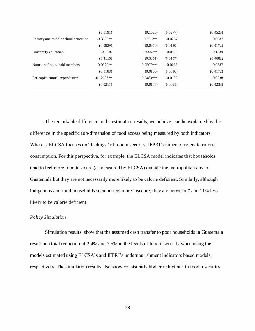
Table 8. Parameter estimates of logistic models for the food insecurity status of households using
data representative of poor households only
Variable Parameter estimates Marginal effects
ELCSA IFPRI’s undernourishment ELCSA IFPRI’s undernourishment
Intercept 2.3822***
(0.2991)
4.3799***
(0.2671)
North -0.7018**
(0.2024)
-1.0444***
(0.1939)
-0.0613
(0.0297)
-0.1613
(0.0715)
Northeast 0.2394
(0.1784)
-0.7124***
(0.1739)
0.0209
(0.0102)
-0.1100
(0.0487)
Southeast 0.3649*
(0.2023)
-1.2372***
(0.1827)
0.0318
(0.0155)
-0.1910
(0.0847)
Central 0.4732**
(0.1824)
-0.9453***
(0.1700)
0.0414
(0.0201)
-0.1459
(0.0647)
Southwest -0.1089
(0.1680)
-1.3377***
(0.1658)
-0.0095
(0.0046)
-0.2065
(0.0915)
Northwest 0.8896**
(0.2858)
-1.8612***
(0.1911)
0.0778
(0.0378)
-0.2874
(0.1274)
Peten 0.5053
(0.3113)
-0.9063
(0.2358)
0.0442
(0.0215)
-0.1399
(0.0620)
Female 0.1904*
(0.1098)
0.0856
(0.0792)
0.0166
(0.0081)
0.0132
(0.0059)
Indigenous 0.4310***
(0.0973)
-0.4620***
(0.0723)
0.0377
(0.0183)
-0.0713
(0.0316)
Rural 0.2805**
(0.1158)
-0.7694***
(0.0905)
0.0245
(0.0119)
-0.1187
(0.0527)
July-August 0.5117**
(0.1463)
-0.1383
(0.1036)
0.0447
(0.00217)
-0.0214
(0.0095)
Rural*July-August -0.6576**
(0.2034)
0.3823**
(0.1036)
-0.0575
(0.0279)
0.0590
(0.0262)
Presence of Children 0.6528*** -0.7676*** 0.0571 -0.1185
23
(0.1191) (0.1020) (0.0277) (0.0525)
Primary and middle school education -0.3063**
(0.0929)
0.2512**
(0.0670)
-0.0267
(0.0130)
0.0387
(0.0172)
University education -0.3686
(0.4116)
0.9967**
(0.3851)
-0.0322
(0.0157)
0.1539
(0.0682)
Number of household members -0.0379**
(0.0188)
0.2507***
(0.0166)
-0.0033
(0.0016)
0.0387
(0.0172)
Per-capita annual expenditures
-0.1205***
(0.0211)
-0.3483***
(0.0177)
-0.0105
(0.0051)
-0.0538
(0.0238)
The remarkable difference in the estimation results, we believe, can be explained by the
difference in the specific sub-dimension of food access being measured by both indicators.
Whereas ELCSA focuses on “feelings” of food insecurity, IFPRI’s indicator refers to calorie
consumption. For this perspective, for example, the ELCSA model indicates that households
tend to feel more food insecure (as measured by ELCSA) outside the metropolitan area of
Guatemala but they are not necessarily more likely to be calorie deficient. Similarly, although
indigenous and rural households seem to feel more insecure, they are between 7 and 11% less
likely to be calorie deficient.
Policy Simulation
Simulation results show that the assumed cash transfer to poor households in Guatemala
result in a total reduction of 2.4% and 7.5% in the levels of food insecurity when using the
models estimated using ELCSA’s and IFPRI’s undernourishment indicators based models,
respectively. The simulation results also show consistently higher reductions in food insecurity

24
as a result of the cash transfer program when using the using IFPRIS’s undernourishment model
across all the regions in the country7.
Figure 3. Percentage reduction in the incidence of food insecurity from a simulated cash transfer
policy.
Despite yielding different quantitative results, both simulation analyses suggest small
reductions in the food insecurity prevalence as a result of the assumed cash transfer which can be
explained by the relatively small magnitude of the per-capital annual expenditure coefficients in
the logistic regression models; thus, only very large cash transfer programs can result in high
levels of reduction in the prevalence of food insecurity, which is not sustainable and neither
efficient for reducing food insecurity in the long run. This also suggest that increasing income
7 The simulation used the “optimal” cutoff points shown in Table 4. When 0.5 is used as the cutoff points
for both models, the simulated average reduction in the prevalence of food insecurity are 0% and 3.1%, for ELCSA
and IFPRI’s models, respectively.
0.0%
2.0%
4.0%
6.0%
8.0%
10.0%
12.0%
Metropolitan North Northeast Southeast Central Southwest Northwest Peten
Percentage change in food insecurity
ELCSA IFPRI's undernourishment

25
alone, via cash transfers for example, may not be an efficient policy for improving food security
and that a holistic approach is necessary if Guatemala is to take important steps towards reducing
the incidence of food insecurity. This holds true independently of the methodology used to
measure food security.
Summary and Conclusions
The main objectives of this study were to measure the prevalence of food insecurity in
Guatemala, to assess factors associated with household food insecurity, and to evaluate the
potential impact of a cash transfer policy when measuring food insecurity using two alternative
food security indicators: ELCSA and IFPRI’s undernourishment. Our results show that even
though both indicators operate in the same dimension of the concept of food security (access)
and at the same level (households), they do not only yield different estimates of the prevalence
of food insecurity, but also differ significantly (in 40% of cases ) when classifying households’
food insecurity status. This disagreement results in differences in the estimates of food insecure
prevalence across regions. Logistic regression models estimated to asses and identify drivers of
household food insecurity also found large differences both in the direction and magnitude of
factors affecting food insecurity using the alternative food security indicators. Finally, policy
simulation results show that cash transfer policies are likely to have only a small effect at
reducing the prevalence of food insecurity. However, more research is needed to evaluate the
cost effectiveness of cash transfers relative to other alternative policies. Although, the
remarkable differences found in the results of the analyses suing both indicators is at first sight
very troubling, it also reflects the fact that each food security dimension (in this case access) is
composed of several sub-dimensions.

26
More work need to assess the external reliability of food security indicators in general.
However, whereas there is some body of literature that has evaluated the use of HES to measure
nutritional outcomes (Fiedler et al., 2012; Jariseta et al., 2012; Smith and Subandoro, 2007)
most of the literature evaluating ELCSA focuses only on its internal reliability; thus, more work
is urgently needed to evaluate this indicator.
Although several arguments can be made in favor or against using one indicator or the
other, including aspects related to implementation costs or reliability, the choice of one indicator
over another should ultimately be based on policy objectives. It is also very important for both
researchers and policy makers to avoid using the two indicators subject of this study, or any
other indicators for that matter, interchangeably. When possible, several alternative food security
indicators within each food security dimension should be used for policy analysis and
implementation.
References
Adato, M. and Hoddinott, J. 2010. Conditional cash transfers in Latin America. The Johns
Hopkins University Press. 386p.
Allison, P. D. 1999. Logistic Regression Using the SAS® System: Theory and Application. Cary,
NC. : SAS Institute Inc.
Carrasco, B., Peinador, R. and Aparicio, R. 2010. La Escala Mexicana de Seguridad Alimentaria
en el ENIGH: evidencias de la relación entre la inseguridad alimentaria y la calidad de dieta en
los hogares mexicanos. Presented at the X national meeting of demographic investigation In
Mexico of the Mexican Society of Demography. Mexico, D.F., 3-6 November of 2010.
Conover, W.J. 1999. Practical nonparametric statistics. 3rd edition. John Wiley &Sons, Inc.
U.S.A., 584p.
Famine Early Warning System (FEWS NET). 2013. Guatemala, Seasonal Calendar. Available
at: http://www.fews.net/central-america-and-caribbean/guatemala
FAO. 2001. Human energy requirements. Report of a joint FAO/WHO/UNU expert consultation.
Rome, 17-24 October 2001.

27
FAO. 1996. World Food Summit. November 13-17, 1996. Rome.
FAO. 2012. Escala Latinoamericana y Caribeña de Seguridad Alimentaria (ELCSA), Manual de
uso y aplicación. 86 p.
FAO, IFAD and WFP. 2015. The State of Food Insecurity in the World. Meeting the 2015
international hunger targets: taking stock of uneven progress. Rome, FAO. 62p.
Fiedler, J. L., Lividini, K., Bermudez, O. I., & Smitz, M. F. (2012). Household Consumption and
Expenditures Surveys (HCES): a primer for food and nutrition analysts in low-and middle-
income countries. Food & Nutrition Bulletin, 33(Supplement 2), 170S-184S.
Greene, W.H. 2012. Econometric Analysis. 7th edition. Prentice Hall, NJ, U.S.A. 1188p.
Haen, H., Klasen, S. and Qaim, M. 2011. What do we really know? Metric for food insecurity
and undernutrition. Food Policy 36: 760-769.
Headey, D. and Ecker, O. 2012. Improving the Measurement of Food Security. IFPRI Discussion
Paper 01225.
Instituto de Nutricion de Centro America y Panama (INCAP). 2012. Tabla de Composicion de
los Alimentos de Centro America. INCAP/OPS, Guatemala. 2nd ed. 137p.
Instituto Nacional de Estadística (INE). 2011. Encuesta Nacional de Condiciones de Vida 2011.
Report. 24p.
Jariseta, Z. R., Dary, O., Fiedler, J. L., & Franklin, N. 2012. Comparison of estimates of the
nutrient density of the diet of women and children in Uganda by Household Consumption and
Expenditures Surveys (HCES) and 24-hour recall. Food & Nutrition Bulletin, 33(Supplement 2),
199S-207S.
Jimenez, A.Z., Prada, G.E. and Herran, O.F. 2012. Escalas para medir la seguridad alimentaria
en Colombia, son validas? Rev Chil Nutr 39(1): 8-17.
Leroy, J.L., Ruel, M., Frongillo, E.A., Harris, J. and Ballard T.J. 2015. Measuring the Food
Access Dimension of Food Security: A Critical Review and Mapping of Indicators. Food and
Nutrition Bulletin 36(2): 167-195.
Maxwell, D., Vaitla, B. and Coates, J. 2014. How do indicators of household food insecurity
measure up? An empirical comparison from Ethiopia. Food Policy 47: 107-116.
Maxwell, D., Coates, J. and Vaitla, B. 2013. How Do Different Indicators of Household Food
Security Compare? Empirical Evidence from Tigray. Feinstein International Center, Tufts
University: Medford, USA.
Melgar Quiñnez, H. and Samayoa, L. 2011. Prevalencia de inseguridad alimentaria del hogar en
Guatemala, Encuesta nacional de condiciones de vida 2011 (ENCOVI). Report: 14p.

28
Pangaribowo, E. H., Gerber, N. and Torero, M. 2013. Food and nutrition security indicators: a
review. Working paper. Center for Development Research, University of Bonn.
Smith, L.C. and Subandoro, A. 2007. Measuring Food Security Using Household Expenditure
Surveys. Food Security in Practice thecnical guide series. Washington, D.C.: International Food
Policy Research Institute.
USDA. 2016. Supplemental Nutrition Assistance Program, Eligibility. Available at:
http://www.fns.usda.gov/snap/eligibility
Valencia-Valero, R.G. and Ortiz-Hernandez, L. 2014. Disponibilidad de alimentos en los
hogares mexicanos de acuerdo con el grado de inseguridad alimentaria. Salud pública de Mexico
56(2): 154-164.
Vega-Macedo, M., Shamah-Levy, T., Peinador-Roldan, R., Mendez-Gomez, I. and Melgar-
Quiñonez, H. 2014. Food insecurity and variety of food in Mexican households with children
under five years. Salud Pública de Mexico 56(1).
World Bank. Living Standards Measurement Studies. Available online at: econ.worldbank.org.
Last visited: October 4, 2016.

29
Annex 1. ELCSA’s questions.
All the questions start with: During the last 3 months, because of lack of money or other
resources,
No. Question in Spanish Translation to English Dimension
1 … ¿alguna vez usted se preocupó
porque los alimentos no se acabaran
en su hogar?
… did you ever worry you may not
have enough food at home?
Concern -
household
2 … ¿alguna vez en su hogar se
quedaron sin alimentos?
… has your household ever been
left without food?
Food quantity -
household
3 … ¿alguna vez en su hogar dejaron de
tener una alimentación sana y
balanceada?
… has your household ever not had
a healthy diet?
Food quantity
and quality -
household
4 … ¿alguna vez usted o algún adulto
en su hogar tuvo una alimentación
basada en poca variedad de
alimentos?
… have you or another adult in
your household ever had a diet
based in poor food variety?
Food quality -
household
5 … ¿alguna vez usted o algún adulto
dejó de desayunar, almorzar o cenar?
… have your or another adult in
your household ever not had
breakfast, lunch or dinner?
Food quantity -
adults
6 … ¿alguna vez usted o algún adulto
en su hogar comió menos de los debía
comer?
… have you or another adult in
your household ever eaten less than
you should?
Food quantity -
adults
7 … ¿alguna vez usted o algún adulto
en su hogar sintió hambre pero no
comió?
… have you or another adult in
your household felt hunger but no
eaten?
Hunger - adults
8 … ¿alguna vez usted o algún adulto
en su hogar solo comió una vez al día
o dejó de comer durante todo un día?
… have you or another adult in
your household ever only eaten
once a day or stopped eating for a
whole day?
Hunger – adults
Survey continues only if the household has children (under 18 years)

30
9 … ¿alguna vez algún menor de 18
años en su hogar dejó de tener una
alimentación saludable y balanceada?
… has anyone under 18 in your
household ever stopped having a
healthy diet?
Quantity and
quality – under
18
10 … ¿alguna vez algún menor de 18
años en su hogar tuvo una
alimentación basada en poca variedad
de alimentos?
… has anyone under 18 in your
household ever had a diet based in
poor food variety?
Food quality –
under 18
11 … ¿alguna vez algún menor de 18
años en su hogar dejó de desayunar,
almorzar o cenar?
… has anyone under 18 in your
household ever stopped having
breakfast, lunch or dinner?
Quantity – under
18
12 … ¿alguna vez algún menor de 18
años en su hogar comió menos de lo
que debía?
… has anyone under 18 in your
household ever eaten less than they
should?
Quantity – under
18
13 … ¿alguna vez tuvieron que disminuir
la cantidad servida en las comidas a
algún menor de 18 años en su hogar?
… have you ever had to reduce the
quantity of food served to anyone
under 18 in your household?
Quantity – under
18
14 … ¿alguna vez algún menor de 18
años en su hogar sintió hambre pero
no comió?
… has anyone under 18 in your
household ever felt hunger but
didn’t eat?
Hunger – under
18
15 … ¿alguna vez algún menor de 18
años en su hogar solo comió una vez
al día o dejó de comer durante todo un
día?
… has anyone under 18 in your
household ever only eaten once a
day or stopped eating for a whole
day?
Hunger – under
18

31
Annex 2. Regions and departments of Guatemala.
No. Region Department
I Metropolitan Guatemala
II North Baja Verapaz
Alta Verapaz
III Northeast
El Progreso
Izabal
Zacapa
Chiquimula
IV Southeast
Santa Rosa
Jalapa
Jutiapa
V Central
Sacatepéquez
Chimaltenango
Escuintla
VI Southwest
Sololá
Totonicapán
Quezaltenango
Suchitepéquez
Retalhuleu
San Marcos
VII Northwest Huhuetenango
Quiché
VIII Peten Petén

32
Source: Judicial body of the republic of Guatemala.

33
Annex 3. Population and food insecurity estimates.
Region Department Population
ELCSA HCES
Difference
(ELCSA -
HCES)
Food
insecurity
estimate
Food insecure
population
Food insecurity
estimate
Food insecure
population
1 Guatemala 3,207,587 0.7049 2,261,028 0.6339 2,033,289 227,739
2 Baja Verapaz 277,380 0.7857 217,937 0.6908 191,614 26,323
2 Alta Verapaz 1,147,593 0.7857 901,664 0.6908 792,757 108,907
3 El Progreso 160,754 0.8113 130,420 0.6556 105,390 25,029
3 Izabal 423,788 0.8113 343,819 0.6556 277,835 65,984
3 Zacapa 225,108 0.8113 182,630 0.6556 147,581 35,049
3 Chiquimula 379,359 0.8113 307,774 0.6556 248,708 59,066
4 Santa Rosa 353,261 0.8599 303,769 0.5776 204,044 99,726
4 Jalapa 327,297 0.8599 281,443 0.5776 189,047 92,396
4 Jutiapa 444,434 0.8599 382,169 0.5776 256,705 125,464
5 Sacatepequez 323,283 0.8589 277,668 0.6029 194,907 82,760
5 Chimaltenango 630,609 0.8589 541,630 0.6029 380,194 161,436
5 Escuintla 716,204 0.8589 615,148 0.6029 431,799 183,348
6 Solola 450,471 0.8458 381,008 0.5875 264,652 116,357
6 Totonicapan 491,298 0.8458 415,540 0.5875 288,638 126,902
6 Quetzaltenango 807,571 0.8458 683,044 0.5875 474,448 208,596
6 Suchitepequez 529,096 0.8458 447,509 0.5875 310,844 136,665
6 Retalhueu 311,167 0.8458 263,185 0.5875 182,811 80,374
6 San Marcos 1,044,667 0.8458 883,579 0.5875 613,742 269,837
7 Huehuetenango 1,173,977 0.9125 1,071,254 0.47 551,769 519,485
7 Quiche 985,690 0.9125 899,442 0.47 463,274 436,168
8 Peten 662,779 0.8824 584,836 0.6755 447,707 137,129
Totals 15,073,373
12,376,496
9,051,756 3,324,741