OptiRisk Systems: White Paper Series Domain: Finance Reference Number: OPT 008

MEASURING PENSION FUND PERFORMANCE USING

RISK-ADJUSTED MEASUREMENTS

Last Update January 2009

Measuring Pension Fund Performance usingRisk-Adjusted Measurements

Katharina Schwaiger Cormac Lucas Gautam Mitra ∗

January 2009

∗CARISMA, School of Information Systems, Computing and Mathematics, Brunel University,Uxbridge, United Kingdom

1

1 Introduction and Background

This report uses risk-adjusted performance measures to identify the quality of al-

ternative decision models. This report uses the decision models introduced by

Schwaiger et al. (2007) and the simulation and decision evaluation outcomes from

Schwaiger et al. (2008).

Risk-adjusted performance measures are used by fund managers to rank and com-

pare their portfolio performance with peers. In this report we examine the perfor-

mance of alternative decision models for pension funds and use two ratios, namely

the Sortino and the Solvency ratio to measure their performance over time.

1.1 Background

In Schwaiger et al. (2007) five different approaches in tackling the pension fund

problem are introduced: a linear deterministic model, a stochastic programming

model, a chance-constrained programming model, an integrated chance-constrained

programming model and a simple fixed mix model. This section reviews the de-

terministic and stochastic models, whose values of the decision variables from the

optimization outcomes are then used to conduct simulation and decision evaluation.

In the deterministic model the model indices are b, which is an element of the

total set of bonds available and t, which is the current time. The objective is to

minimize the total deviations between the bonds and liabilities PV 01 values and

at the same time minimise initial injected cash. The decision variables are:

The model indices are:

b bond from a bond set B

t time horizon 1, ..., T

2

Secondly, we define the parameters:

Lt liability value at time t

LPV 01t PV01 value of the liability at time t

BPV 01bt PV01 value of bond b at time t

cbt cash flow stream of bond b at time t

Pb trading price of bond b

α transaction cost involved when bonds are sold or bought

Ob opening position of bond b at the initial time period

rt interest rate at time t

Now we define the decision variables. All variables are constrained to be nonnegative.

xb amount of bond b purchased

yb amount of bond b sold

zb amount of bond b held

dt amount borrowed at time period t; limited to be ≤ Mt ∀tst amount lent at time period t

C initial available cash

Furthermore, we use the following decision variables to measure the deviations of the assets PV 01 and the liabilities PV 01:

devot measurement of over deviation at time t

devut measurement of under deviation at time t

The set of constraints include some basic constraints for portfolio optimization:

these are the cash-flow accounting equation and the inventory balance constraints.

The cash-flow accounting equation initializes the new asset portfolio by liquidating

the old asset allocation and including the available cash C.

3

B∑

b=1

(1 + α)Pbxb ≤ C +B∑

b=1

(1− α)Pbyb (1)

The inventory balance constraint assures that the holding of bond b is made up

of the opening position of the same bond including the amount bought minus the

amount sold:

zb = Ob + xb − yb ∀ b (2)

The following constraints match the bonds cash flows with the liabilities stream,

having the possibility to borrow from the bank or reinvest spare cash. At the final

time period there is no opportunity to borrow from the bank anymore.

B∑

b=1

cb1zb + d1 = L1 + s1 (3)

B∑

b=1

cbtzb + dt − (1 + rt)dt−1 = Lt + st − (1 + rt)st−1 t : 2 ≤ t ≤ T (4)

B∑

b=1

cbT zb − (1 + rT )dt−1 = LT + sT − (1 + rT )st−1 (5)

Furthermore, we define the behavior of the variables devot and devut with the

following constraint that binds them to the difference of the assets and liabilities

PV 01 values:

B∑

b=1

BPV 01btzb = devot − devut + LPV 01t ∀ t (6)

If we include the minimum and maximum amount of bonds in the portfolio within

a specific rating class, say AAA rating, specified by the pension fund, we get the

4

following user specific constraints:

MinInRatingclassAAA ≤∑

bonds

zb(i=AAA,.,.,.)t ≤ MaxInRatingclassAAA ∀ t (7)

Similar limits are imposed in respect of other bond characteristic, that is country,

issuer and sector.

An increased need of initial cash means an increase in the active members’ contri-

butions. The first objective function is the initial cash, which has to be injected in

advance to achieve a (feasible) matching between assets and liabilities:

φ1(dt) = Minimize C +T∑

t=1

dt (8)

The second objective function is the total deviations of assets and liabilities; there

are other suitable objective functions we might consider depending on the decision

values required.

The objective function minimizes the total PV 01 deviations of assets and liabili-

ties. This linear objective function is given by

φ2(devot, devut) = Minimize

T∑t=1

(devot + devut). (9)

In the two-stage stochastic programming models (including the chance-constrained

and integrated chance-constrained programming models) the uncertainty is repre-

sented in interest rate scenarios. The objective is to minimize the total present

value deviations of assets and liabilities and at the same time minimizing initial

injected cash.

5

The sets:

b bond from a bond set B

t time horizon 1, ..., T

s scenario 1, ..., S

The parameters:

cbt cash flow stream of bond b at time t

Pb trading price of bond b

α bid-ask spread in percentage when bonds are sold or bought

Ob opening position of bond b at the initial time period

γt weight of liabilities with respect to the asset value at time t; likely to be > 1

can be user defined with high values at the earlier time points

and then decreasing with time

βt reliability level at time t; likely to be > 0;

can be user defined or assumed to be constant over time

λt maximum expected shortfall in fraction of the liabilities at time t;

again user defined or assumed to be constant

N sufficiently large number for the chance constraint

(maximum value the investment portfolio is likely to reach)

The stochastic parameters:

Lst liability value at time t under scenario s

rst uncertain interest rate at time t

πs probability of scenario s occurring, equiprobable

LPV st uncertain present value of the liability at time t

BPV b,st uncertain present value of bond b at time t

The implementable first stage decision variables:

xb amount of bond b purchased

6

yb amount of bond b sold

zb amount of bond b held

C initial cash

The following are the non-implementable stochastic decision variables:

dst uncertain amount borrowed at time period t; limited to be ≤ Mt ∀t

sst uncertain amount lent at time period t

shortagest amount of underfunding at time t

δst binary variable, which takes the value of 1 if there is any underfunding

The constraints:

cash-flow accounting equation:

B∑

b=1

(1 + α)Pbxb ≤ C +B∑

b=1

(1− α)Pbyb (10)

Inventory balance equation:

zb = Ob + xb − yb ∀ b (11)

Matching equations for all time periods:

B∑

b=1

cb1zb + ds

1 = Ls1 + ss

1 ∀ s (12)

B∑

b=1

cbtzb + ds

t − (1 + rt)dst−1 = Ls

t + sst − (1 + rt)s

st−1 ∀ s, t ≥ 2 (13)

7

B∑

b=1

cbT zb − (1 + rT )ds

T−1 = LsT + ss

T − (1 + rT )ssT−1 ∀ s (14)

Non-Anticipativity constraints:

ds1 = d1

1 s = 2, ..., S (15)

ss1 = d1

1 s = 2, ..., S (16)

The chance constraints are formulated as follows:

P{B∑

b=1

BPV sb,t+1zb + PV ss

t+1 − γLPV st+1 − γPV ds

t+1 ≥ 0 | (t, s)} ≥ βt ∀ t (17)

Nδst+1 ≥ γLPV s

t+1 + γPV dst+1 −

B∑

b=1

BPV sb,t+1zb − PV ss

t+1c, (18)

πs

S∑s=1

δst+1 ≤ 1− βt ∀ t (19)

N(1− δst+1)−

1

N≥ BPV s

b,t+1zb + PV sst+1 − γLPV s

t+1 − γPV dst+1 ∀ t, s (20)

δst ε{0, 1} ∀ t (21)

The integrated chance constraints can be included in the following way:

B∑

b=1

BPV sb,tzb + PV ss

t − γLPV st − γPV ds

t + shortagest ≥ 0 ∀t, s (22)

π

S∑s=1

shortagest ≤ λmaxs(LPV s

t ) ∀t (23)

8

The objective functions are:

φ5(dst) = Minimize C +

T∑t=1

S∑s=1

πs(dst) (24)

and:

φ6(devost , devus

t) = Minimize

T∑t=1

S∑s=1

πs(devost + devus

t) (25)

2 Risk-Adjusted Performance Measures

The performance of any fund can be measured using different measurement. We in-

troduce the most used ones: from academia: (1) the standard deviation of returns,

(2) the Sharpe ratio (see also Sharpe, 1966 and 1994), (3) Value at Risk, (4) the

Jensen Index and from industry practice: (5) the Sortino ratio, (6) the Treynor ra-

tio, (7) the Modigliani or M-Square Measure (see Modigliani and Modigliani 1997)

and (8) the Morningstar Rating:

1. As financial interpretation, the standard deviation of a fund represents its

risk. Fund Managers look at the standard deviation of excess return over the

risk free rate or some benchmark. The standard deviation of the difference

between the funds return and a benchmark return is also called the tracking

error. The higher the standard deviation, the higher the expected return for

an investment and the more risk bearing the investor.

The standard deviation can be calculated the following way:

σ =

√√√√ 1

N

N∑i=1

(xi − x)2 (26)

9

where x is the mean of return and N is the number of observations.

2. The Sharpe ratio (or Sharpe index) measures the excess return per unit of

risk in the investment. All models have the same benchmark and the fund

manager will choose the investment with the highest Sharpe ratio.

The ex ante Sharpe ratio is given as follows:

S ≡ d

σd

, (27)

where d is the expected value of the differential return of the fund and a

benchmark, i.e.

d ≡ E[RP −RI ]

and σd is the predicted standard deviation of d, which is the forthcoming

differential return.

The ex post Sharpe ratio is as follows:

Sh ≡√

D

σD

, (28)

where

Dt ≡ RPt −RIt

D ≡ 1

T

T∑t=1

Dt

σD ≡√∑T

t=1(Dt −D)2

T − 1

10

3. Value at Risk (VaR) measures the least expected loss (relative to wealth)

that will be expected given a certain possibility (confidence level).

Value at Risk can be calculated as follows (see Gaivoronski 2005):

V aR(W ) = E(W )− inf{u : F (u) > α} (29)

where α is the quantile of return and 1− α is the confidence level.

4. The Jensen Index measures the performance against the market index. A

high Jensen Index is interpreted as higher return given a risk level on the

portfolio.

The Jensen Index is gvien by (see Jensen 1969):

J = RP − rf − β(RI − rf ) (30)

The Treynor ratio T is given by:

T =RP − rf

β, (31)

where RP is the portfolio return, rf is the risk free rate and β = Cov(RP ,RM )V ar(RM )

is the portfolio β with respect to the market.

5. The Sortino Ratio roots from the Sortino Ratio, but it is industry widely

used since it only penalizes a portfolios underperformance via the downside

deviation.

The Sortino ratio is calculated by:

S ≡ RP −RI

σd

, (32)

11

where

RP ≡ (N∏

i=1

(1 + RPi))1N − 1

σd ≡

√√√√ 1

N

N∑i=1

(min(RPi −RI , 0))2

The term σd is also called the downside deviation or target semideviation.

6. The Treynor ratio measures the returns earned in excess of which could be

earned on a riskless investment. The higher the Treynor ratio, the better the

performance of the fund strategy. Like the Sharpe ratio, the Treynor ratio

is based on the capital asset pricing model (CAPM), which means that any

investor can achieve any level of risk by investing in the fund with the highest

Sharpe ratio regardless of his/her degree of risk aversion.

7. Modigliani et al. propose an alternative measure which is easy to interpret as

a fund manager. The Modigliani measure evaluates in basis points, how much

a portfolio out- or underperformed the market. The higher the Modigliani

Measure, the higher the fund’s return for any level of risk.

The Modigliani or M-Square Measure (see Modigliani and Modigliani

1997) is given as the following:

RAPA(F ) =σI

σF

eF (33)

where RAPA stands for Risk-adjusted performance,σI and σF are the stan-

dard deviation of the Benchmark excess return and the Fund’s excess return,

respectively, and eF is the Fund’s average excess return.

8. Fund Managers often use the star rating or Morningstar Rating from Morn-

ingstar Inc. which classifies funds into five ratings. To obtain these rating

12

they use their own risk return measures.

For the Morningstar Ratings, the excess return of a bond fund is calculated

adjusting for sales loads and subtracting the 90 day Treasury bill rate.

MorningstarReturn =SalesLoadAdjustedExcessReturn− 90dayTreasuryBillReturn

AverageExcessReturnforBondFundClass(34)

The fund return is adjusted for maximum front-end loads, applicable deferred

loads and applicable redemption fees. The top 10% of the funds receive a 5

star Rating, the next 22.5% receive 4 Stars, next 35% 3 Stars, next 22.5% 2

Stars and the last 10% 1 Star.

MorningstarRisk =Fund′sAverageUnderperformance

AverageUnderperformanceofBondFundClass(35)

An additional method to evaluate the performance of the different models is look-

ing at the solvency ratio:

Solvency =wealth− technicalreserves

technicalreserves(36)

Assumptions about Input Variables

For

calculating the Solvency and the Sortino ratio, the following assumptions are made:

Variable Used Input Description/Explanation

wealth Total Inflows Portfolio asset wealth and saved cash

technicalreserves Total Outflows Liability Value and amount borrowed

RP Portfolio Return Portfolio return generated from assets and cash

RI

Liabilities are meant to be matched,

Liability Return which makes them the benchmark to be metThe aim of the models is to match the liabilities stream with a bond portfolio,

where over- and underdeviations are penalized equally. From the ratios we aim to

have inflows = outflows, which makes the numerator in the solvency ratio equal

to zero and the same in the Sortino ratio. For matching strategies both ratios

reflect good results if they are close to zero. For the further sections only the

Sortino and the Solvency ratios are used.

13

3 Hypotheses Testing

Hypothesis testing is used to decide statistically about the computational results

of this work. There are five steps involved: (a) Identifying the null hypothesis:

H0 : µX = y, where y is the value to be tested for. The test is used to find out if

the mean of the Sortino and Solvency ratios are equal to zero, where µX is the

mean of the Sortino and Solvency Ratio of the model X with X being the SP,

CCP or ICCP model. The three possible alternative hypothesis and their critical

region, where we reject H0 are:

H1 : µX > y t =X − µ0

S/√

n> tα,d.f. (37)

H1 : µX < y t =X − µ0

S/√

n< −tα,d.f. (38)

H1 : µX 6= y |t| = X − µ0

S/√

n> tα/2,d.f. (39)

The second step (b) is to choose a rejection level α, which is normally 1% or 5%.

Then (c) we select a test statistic (t-test in this case) and calculate its value form

the sample data, which is called the observed value of the test statistic. We then

(d) compare the observed value to the critical value obtained for the α level. And

the last step (e) is to make a decision if either to accept the null hypothesis or if

to reject it and accept the alternate hypothesis.

4 Computational Investigation

Two ratios are used to measure the portfolios performance: the Solvency ratio and

the Sortino ratio. The solvency ratio is easily computed and widely understood.

The Sortino ratio is an extension of the Sharpe ratio, where as a measure of risk

the semi-standard deviation is used. The semi-variance only uses the probability

of shortfall, unlike variance, which accounts for positive and negative outcomes

14

equally. The following graph (Figure 1) shows the Solvency and the Sortino ratios

for the SP, CCP and ICCP models. The higher the ratios the better, but in case

of matching, where the liabilities are the benchmark and outperformance is

penalized, both ratios reflect good results when they are close to zero.

Figure 1: Solvency and Sortino Ratios for the SP, CCP and ICCP Model

From Figure 1 it can be seen that the SP model has a solvency ratio close to zero

for half the time periods and then it increases in the other half, the CCP has a

downward sloping solvency ratio, which means that the liabilities are growing

faster than the assets and finally, the ICCP model has a very smooth solvency

ratio close to zero for all time periods, which means that the assets match the

liabilities nearly perfectly. The second graph explains a bit more: the SP model

has an upward sloping Sortino ratio, which means that above zero the risk of

making big losses gets smaller and that the assets outperform the liabilities, the

15

CCP model has at some points in time a high risk of making a big loss when

looking at its Sortino ratio, while again the ICCP is close to zero which means it

is closely matching the liabilities.

Hypothesis Testing

The models are further analyzed using hypothesis testing, where there are three

different null hypothesis:

H0 : µICCP = 0 (40)

µCCP = 0 (41)

µSP = 0 (42)

and the corresponding alternate hypothesis:

H1 : µICCP 6= 0 (43)

µCCP 6= 0 (44)

µSP 6= 0 (45)

Table 1 shows the t-test statistics for the three null hypothesis for each ratio. For

the CCP Solvency and CCP and ICCP Sortino ratio there is no evidence at all to

accept the null hypothesis, while at 0.3%, 2.5% and 7% (2-tailed) we accept the

null hypothesis for the SP Solvency, Sortino and ICCP Solvency ratio to have a

mean of zero.

Stress Testing High/Low Interest Rates

The next set of graphs show the surplus/deficit frequency distribution at four

different time periods: t = 2, t = 10, t = 20 and t = 40 for all four models. The

following results (Figure 2 and Figure 3) show the surplus/deficit frequency

distribution of the SP model using high and low interest rate scenarios. The SP

model performs relatively well (in matching terms) compared to the other models

and in both cases of high and low interest rate scenarios.

16

Table 1: Hypothesis Testing of the Ratios

17

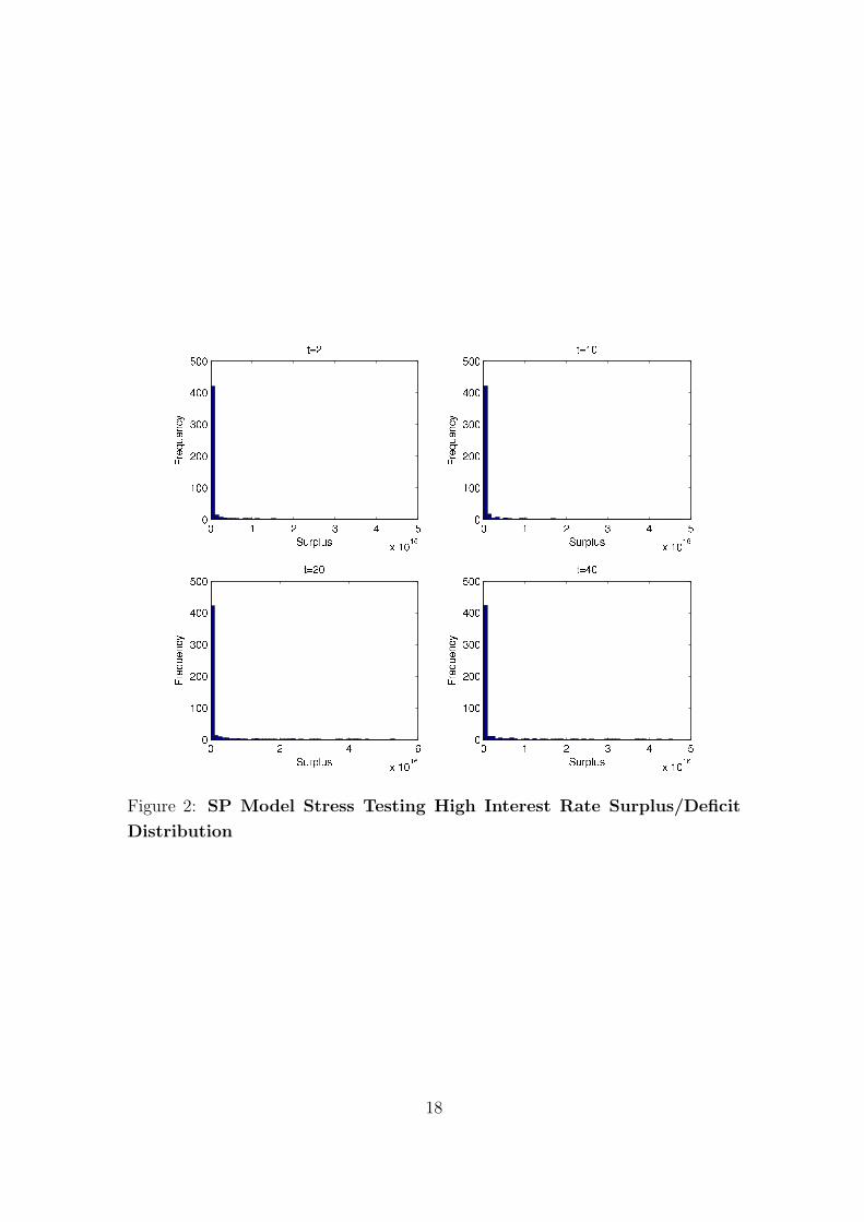
Figure 2: SP Model Stress Testing High Interest Rate Surplus/Deficit

Distribution

18

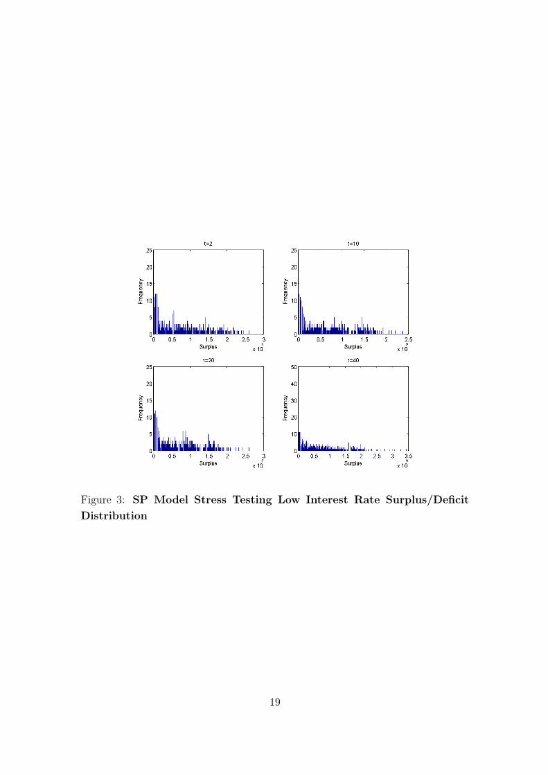
Figure 3: SP Model Stress Testing Low Interest Rate Surplus/Deficit

Distribution

19

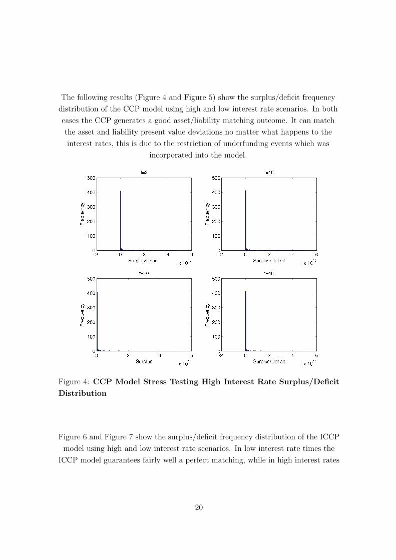
The following results (Figure 4 and Figure 5) show the surplus/deficit frequency

distribution of the CCP model using high and low interest rate scenarios. In both

cases the CCP generates a good asset/liability matching outcome. It can match

the asset and liability present value deviations no matter what happens to the

interest rates, this is due to the restriction of underfunding events which was

incorporated into the model.

Figure 4: CCP Model Stress Testing High Interest Rate Surplus/Deficit

Distribution

Figure 6 and Figure 7 show the surplus/deficit frequency distribution of the ICCP

model using high and low interest rate scenarios. In low interest rate times the

ICCP model guarantees fairly well a perfect matching, while in high interest rates

20

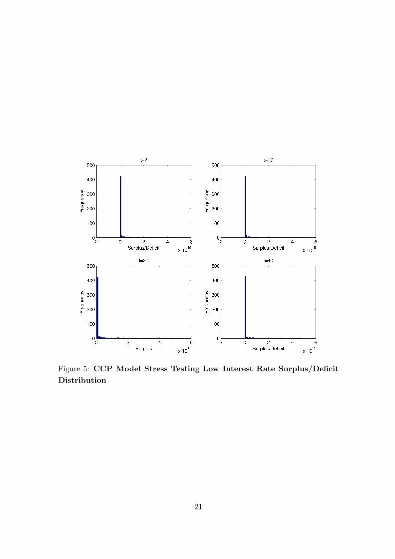
Figure 5: CCP Model Stress Testing Low Interest Rate Surplus/Deficit

Distribution

21

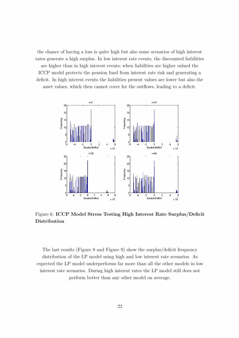
the chance of having a loss is quite high but also some scenarios of high interest

rates generate a high surplus. In low interest rate events, the discounted liabilities

are higher than in high interest events; when liabilities are higher valued the

ICCP model protects the pension fund from interest rate risk and generating a

deficit. In high interest events the liabilities present values are lower but also the

asset values, which then cannot cover for the outflows, leading to a deficit.

Figure 6: ICCP Model Stress Testing High Interest Rate Surplus/Deficit

Distribution

The last results (Figure 8 and Figure 9) show the surplus/deficit frequency

distribution of the LP model using high and low interest rate scenarios. As

expected the LP model underperforms far more than all the other models in low

interest rate scenarios. During high interest rates the LP model still does not

perform better than any other model on average.

22

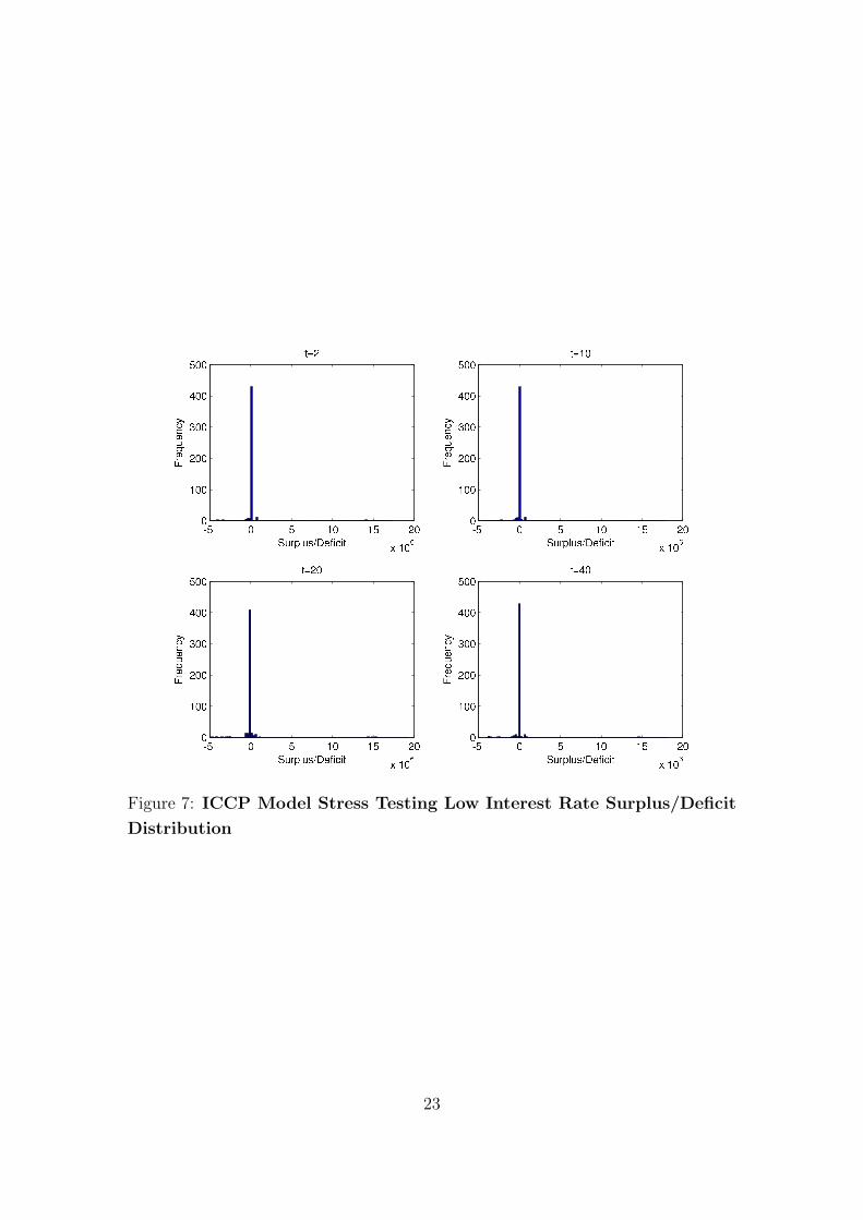
Figure 7: ICCP Model Stress Testing Low Interest Rate Surplus/Deficit

Distribution

23

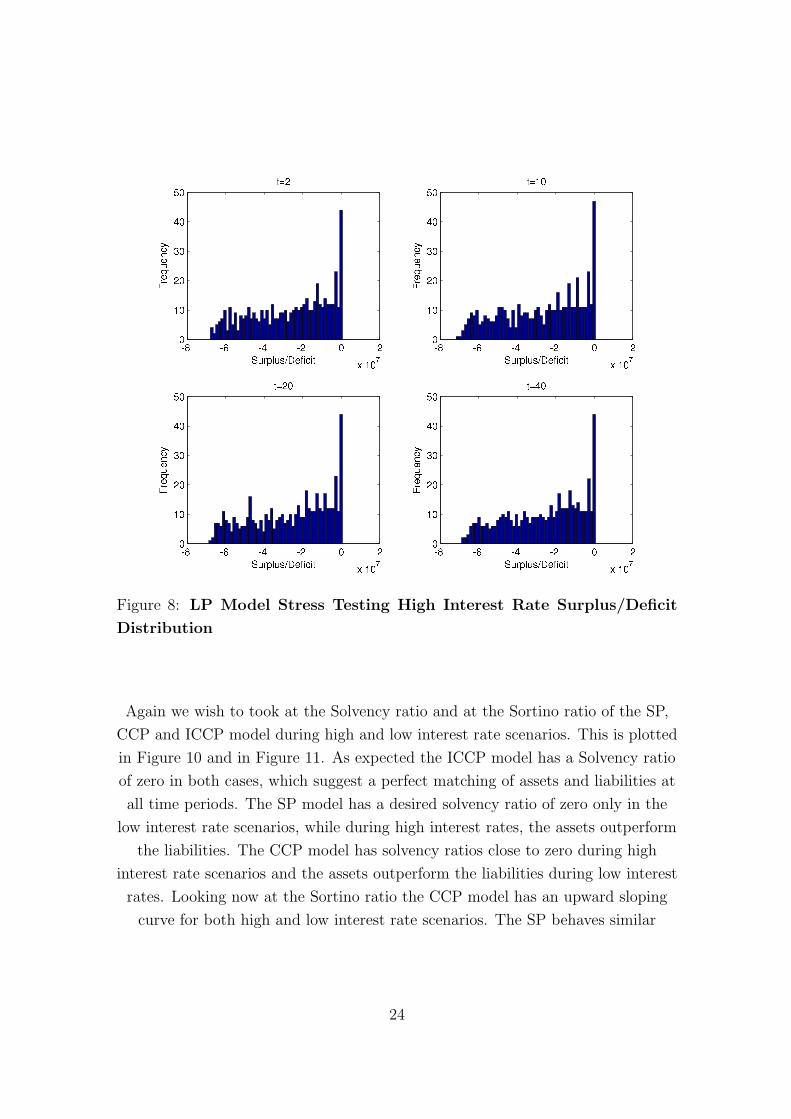
Figure 8: LP Model Stress Testing High Interest Rate Surplus/Deficit

Distribution

Again we wish to took at the Solvency ratio and at the Sortino ratio of the SP,

CCP and ICCP model during high and low interest rate scenarios. This is plotted

in Figure 10 and in Figure 11. As expected the ICCP model has a Solvency ratio

of zero in both cases, which suggest a perfect matching of assets and liabilities at

all time periods. The SP model has a desired solvency ratio of zero only in the

low interest rate scenarios, while during high interest rates, the assets outperform

the liabilities. The CCP model has solvency ratios close to zero during high

interest rate scenarios and the assets outperform the liabilities during low interest

rates. Looking now at the Sortino ratio the CCP model has an upward sloping

curve for both high and low interest rate scenarios. The SP behaves similar

24

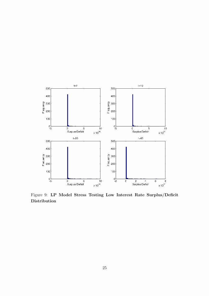
Figure 9: LP Model Stress Testing Low Interest Rate Surplus/Deficit

Distribution

25

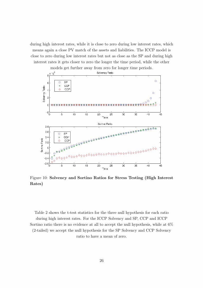
during high interest rates, while it is close to zero during low interest rates, which

means again a close PV match of the assets and liabilities. The ICCP model is

close to zero during low interest rates but not as close as the SP and during high

interest rates it gets closer to zero the longer the time period, while the other

models get further away from zero for longer time periods.

Figure 10: Solvency and Sortino Ratios for Stress Testing (High Interest

Rates)

Table 2 shows the t-test statistics for the three null hypothesis for each ratio

during high interest rates. For the ICCP Solvency and SP, CCP and ICCP

Sortino ratio there is no evidence at all to accept the null hypothesis, while at 6%

(2-tailed) we accept the null hypothesis for the SP Solvency and CCP Solvency

ratio to have a mean of zero.

26

Figure 11: Solvency and Sortino Ratios for Stress Testing (Low Interest

Rates)

27

Table 3 shows the t-test statistics for the three null hypothesis for each ratio

during low interest rates. For the SP Solvency and SP, CCP and ICCP Sortino

ratio there is no evidence at all to accept the null hypothesis, while at 6% and

81.8% (2-tailed) we accept the null hypothesis for the CCP Solvency and ICCP

Solvency ratio to have a mean of zero.

28

Table 2: Hypothesis Testing of the Ratios in Stress Testing (High Interest Rates)

29

Table 3: Hypothesis Testing of the Ratios in Stress Testing (Low Interest Rates)

30

5 Conclusions

This report showed how to measure and evaluate portfolio performances. A

collection of risk-adjusted measurements from both academia and industry were

explained; of which two of them were used to evaluate a stochastic asset and

liability management model: namely the Sortino ratio and the Solvency ratio. By

using hypothesis testing, which is a classical statistical method the outcome of

the ratios is further examined.

31

References

[1] A.A. Gaivoronski and G. Pflug. Value at Risk in Portfolio Optimization: Prop-

erties and Computational Approach. Journal of Risk, 7(2):1–31, 2005.

[2] M.C. Jensen. Risk, The Pricing of Capital Assets, and The Evaluation of

Investment Portfolios. Journal of Business, 42(2):167, 1969.

[3] F. Modigliani and L. Modigliani. Risk-Adjusted Performance. Journal of Port-

folio Management, 23(2):45–54, 1997.

[4] K.J. Schwaiger, G. Mitra, and C. Lucas. Models and Solution Methods for

Liability Determined Investment, 2007.

[5] K.J. Schwaiger, G. Mitra, and C. Lucas. Evaluation and Simulation of Liability

Determined Investment Models, 2008.

[6] W.F. Sharpe. Mutual Fund Performance. The Journal of Business, 39(1):119–

138, 1966.

[7] W.F. Sharpe. The Sharpe Ratio. Journal of Portfolio Management, 21(1):49–

58, 1994.

32