measuring interest rate risk in the treasury operations of an international industrial company

0

MASTER THESIS IN BUSINESS ADMINISTRATION

International Business and Economics Programme

Measuring Interest Rate Risk in the Treasury Operations of an

International Industrial Company Group

A Case Study of Toyota Industries Finance International

Erik Håkansson

Viktor Åberg

Tutors:

Bo Sjö (LiU)

Bo-Arne Karlsson (TIFI)

Jonas Persson (TIFI)

Spring semester 2012

ISRN: LIU-IEI-FIL-A--12/01207--SE

1

Measuring Interest Rate Risk in the Treasury Operations of an International Industrial Company Group

– A Case Study of Toyota Industries Finance International

Authors:

Erik Håkansson & Viktor Åberg

Tutor:

Bo Sjö (LiU)

Bo-Arne Karlsson (TIFI)

Jonas Persson (TIFI)

Publication type:

Thesis in Business Administration

International Business and Economics Programme

Advanced level, 30 credits

Spring semester 2012

ISRN: LIU-IEI-FIL-A--12/01207--SE

Linköping University

Department of Management and Engineering (IEI)

www.liu.se

Contact information, authors:

Erik Håkansson : 0702-43 07 48, [email protected]

Viktor Åberg : 0733-89 63 11, [email protected]

© 2012 Erik Håkansson and Viktor Åberg

2

Abstract

Title: Measuring interest rate risk in the treasury operations of an international industrial company

group – a case study of Toyota Industries Finance International

Authors: Erik Håkansson and Viktor Åberg

Supervisors: Bo Sjö (LiU), Bo-Arne Karlsson (TIFI) and Jonas Persson (TIFI)

Background: The volatility in the interest rate market have increased during the last decade and this

have made interest rate risk management more important for both financial institutions and non-

financial companies with short- and long term financial commitments.

Objective: The main objective of this thesis is to analyze different ways of measuring interest rate risk

in the treasury operations an international industrial company group. Further, the study will also

examine the way treasury departments of international industrial company group’s measure interest

rate risk and explain why this method have been chosen.

Method: The research method of the thesis is a case study and a mix of both quantitative and

qualitative data has been used to conduct it. The quantitative data have been secondary data received

from TIFI’s treasury management software and the qualitative data have been collected through a

survey with eight treasury managers from other international industrial company groups.

Conclusion: The repricing model is suitable because it is straight forward, fairly easy to communicate

to management and it focuses on the book value. However, defining relevant time buckets might be

difficult. The duration model is a good measurement tool because it can be used in a variety of ways,

but a disadvantage is that it focuses on the market value, which might not be appropriate for treasury

departments. Stress testing captures the true change in market value, but demands forecasts about

future interest rate movements and lacks tools to manage the interest rate risk.

Treasury departments of international industrial company groups use a variety of measurement

methods. The most frequently used methods are duration-, maturity- and Value at Risk models and

different kinds of stress tests. The method should not only measure the interest rate risk in a correct

way but it should also be easily explained to management and other executives in the company that

might not have knowledge about financial economics.

The main difference between treasury departments and commercial banks is that commercial banks try

to earn money on interest rate fluctuations, whereas treasury departments want to minimize the impact

of interest rate fluctuations in order to support the company group’s core business.

Key words: Interest rate risk, treasury department, duration model, convexity, repricing model, stress

test

3

Sammanfattning

Titel: Att mäta ränterisk i en internationell industrikoncerns finansavdelning – en fallstudie av Toyota

Industries Finance International

Författare: Erik Håkansson och Viktor Åberg

Handledare: Bo Sjö (LiU), Bo-Arne Karlsson (TIFI) och Jonas Persson (TIFI)

Bakgrund: Under det senaste decenniet har volatiliteten på räntemarknaden blivit större och detta har

lett till att mätningen av ränterisk har blivit viktigare för båda finansiella och icke-finansiella företag

med kort- och långsiktiga finansiella åtaganden.

Syftet: Huvudsyftet med denna uppsats är att analysera olika sätt att mäta ränterisk i internationella

industriföretags finansavdelningar. Vidare ska uppsatsen undersöka hur internationella industriföretags

finansavdelningar mäter ränterisk samt förklara varför de valt den metoden de använder.

Metod: Studiens forskningsmetod är en fallstudie och en blandning av både kvantitativ och kvalitativ

data har använts. Den kvantitativa datan består av data från TIFI’s treasury-programvara och den

kvalitativa datan har samlats in genom en undersökning som skickats till åtta beslutsfattare på olika

finansavdelningar på internationella industrikoncerner.

Slutsats: Repricing model är passande eftersom den är enkel att förklara för en styrelse samt för att

den fokuserar på bokförda värden. Det kan dock vara svårt att välja relevanta tidsfickor.

Durationsmodellen är ett bra mätinstrument då den kan användas på flera olika sätt men den har dock

nackdelen att den fokuserar på marknadsvärdet, vilket inte alltid är lämpligt för en finansavdelning.

Ett stresstest visar den riktiga förändringen i marknadsvärde men kräver prognoser om de framtida

ränteförändringarna och saknar de verktyg som behövs för att hantera ränterisken.

Finansavdelningar på internationella industrikoncerner använder flera olika mätmetoder. De vanligaste

är duration-, maturity-, och Value at Risk-modeller samt olika typer av stresstest. Metoden ska inte

bara mäta ränterisken på ett korrekt sätt utan ska också vara enkel att förklara för styrelser och andra

beslutsfattare i ett företag som kanske inte har kunskaper i finansiell ekonomi.

Den största skillnaden mellan en finansavdelning och en affärsbank är att affärsbanker försöker tjäna

pengar på ränteförändringar, medan finansavdelningar snarare försöker minimera effekten av

räntefluktuationer för att bättre ge stöd åt koncernens kärnverksamhet.

Nyckelord: Ränterisk, treasury, duration, konvexitet, repricing, stresstest

4

Acknowledges

The scope of this thesis is 30 credits and was written during the spring of 2012 in Linköping and

Mjölby.

We would like to thank our supervisor Bo Sjö and our opponents for their insightful comments and

constructive criticism which have improved this thesis. We would also like to thank the respondents of

the survey for their valuable information about how a treasury department practically works and deal

with interest rate risk on a daily basis.

Further, we want to thank our supervisors on TIFI, Bo-Arne Karlsson and Jonas Persson, and the rest

of the treasury department group for the opportunity of writing this thesis and for their assistance when

we have faced problems. We hope that we with this thesis can contribute to their daily work with

interest rate risk management.

Thank you!

Linköping May 23rd

2012

Erik Håkansson Viktor Åberg

5

Table of contents

1 Introduction ........................................................................................................................................ 1

1.1 Background ................................................................................................................................... 1

1.2 Problem discussion ........................................................................................................................ 3

1.3 Objective ....................................................................................................................................... 4

1.4 Methodology ................................................................................................................................. 5

1.5 Delimitations ................................................................................................................................. 5

1.6 Target audience ............................................................................................................................. 5

1.7 Disposition..................................................................................................................................... 5

2 Methodology........................................................................................................................................ 6

2.1 Research method ........................................................................................................................... 6

2.2 Case study as a research method ................................................................................................... 7

2.3 Reliability and validity .................................................................................................................. 8

2.4 Collection of data .......................................................................................................................... 9

2.4.1 Interviews ............................................................................................................................. 10

3 Theoretical framework .................................................................................................................... 12

3.1 Treasury management ................................................................................................................. 12

3.2 Financial institutions ................................................................................................................... 12

3.3 What is interest rate risk? ............................................................................................................ 13

3.3.1 Definition .............................................................................................................................. 13

3.3.2 Types of interest rate risks .................................................................................................... 13

3.4 The term structure ....................................................................................................................... 15

3.5 The repricing model .................................................................................................................... 15

3.5.1 Optimal gap .......................................................................................................................... 17

3.5.2 The choice of time periods ................................................................................................... 17

3.5.3 Imprecise time period on specific assets and liabilities ........................................................ 18

3.5.4 Weaknesses of the repricing model ...................................................................................... 18

3.6 Duration analysis ......................................................................................................................... 19

3.6.1 Duration ................................................................................................................................ 19

6

3.6.2 Modified and dollar duration ................................................................................................ 20

3.6.3 Duration gap ......................................................................................................................... 21

3.6.4 Disadvantages with the duration model................................................................................ 23

3.6.5 Convexity ............................................................................................................................. 23

3.7 Interest rate swaps ....................................................................................................................... 26

3.7.1 Duration of different derivatives .......................................................................................... 26

3.8 Stress testing ................................................................................................................................ 27

3.9 Other types of interest rate risk measures .................................................................................... 28

3.9.1 Maturity ................................................................................................................................ 28

3.9.2 Fixed-to-floating ratio .......................................................................................................... 28

3.9.3 Value at Risk ........................................................................................................................ 29

4 Emipirical data & analysis .............................................................................................................. 30

4.1 Toyota Industries Finance International AB ............................................................................... 30

4.2 Other treasury departments of international industrial company groups..................................... 30

4.3 The empirical approach ............................................................................................................... 31

4.4 Repricing model .......................................................................................................................... 33

4.5 Duration ....................................................................................................................................... 35

4.6 Stress test ..................................................................................................................................... 40

4.7 Maturity ....................................................................................................................................... 40

4.8 Fixed-to-floating ratio ................................................................................................................. 41

5 Discussion .......................................................................................................................................... 42

5.1 Measurement of interest rate risk in treasury departments of other industrial company groups .............. 42

5.2 Differences between commercial banks and treasury departments ............................................. 42

5.3 Duration ....................................................................................................................................... 43

5.4 Stress testing ................................................................................................................................ 45

5.5 Repricing model .......................................................................................................................... 47

5.6 Other measures ............................................................................................................................ 48

5.6.1 Maturity ................................................................................................................................ 48

5.6.2 Fixed-to-floating ratio .......................................................................................................... 48

7

6 Conclusion ......................................................................................................................................... 49

References ............................................................................................................................................ 51

Appendix .............................................................................................................................................. 55

8

Tables

Table 1. Repricing gaps (Million SEK) ................................................................................................. 16

Table 2. Interest rate shocks .................................................................................................................. 32

Table 3. Repricing analysis of 2008-10-22 ........................................................................................... 33





Table 8. Duration analysis of 2008-10-22 ............................................................................................. 36

Table 9. Duration analysis of 2008-12-02 ............................................................................................. 37

Table 10. Duration analysis of 2008-12-03 ........................................................................................... 37



Table 13. Stress test ............................................................................................................................... 40

Table 14. Maturity profile ..................................................................................................................... 40

Table 15. Fixed-to-floating ratio ........................................................................................................... 41

Figures

Figure 1. Notional amounts of interest rate derivatives ........................................................................... 1

Figure 2. Slopes of the yield curve ........................................................................................................ 15

Figure 3. The relationship between duration and convexity ................................................................. 24

Figure 4. Interest rate shocks ................................................................................................................. 32

1

1 Introduction

This chapter will introduce the reader to the background of the thesis. It will discuss the theoretical

problem with interest rate risk for non-financial companies and establish the object and issue of the

paper. Finally this introducing chapter will point out the delimitations and describe the methodology

used and discuss its shortcomings and benefits.

1.1 Background

The last years’ volatility in the financial markets has made risk management more important for all

types of businesses. Further, low interest rates all over the world have forced the financial industry to

develop advanced derivatives to meet the increasing demand for higher returns due to this. According

to experts, this was one of the main causes to the financial crisis that paralyzed the financial sector in

2008 and that later lead to the debt crisis we are currently experiencing.1 In addition to this there are

other reasons to why risk management has grown in importance. Söderlind argues that the

development of the information technology and globalization of the financial markets have made

companies more sensitive to external shocks and that this have made risk measurement even more

important. He also states that new regulations and accounting standards have pushed the development

of risk measurement forward.2

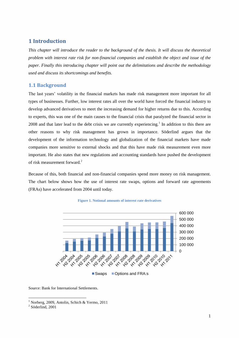
Because of this, both financial and non-financial companies spend more money on risk management.

The chart below shows how the use of interest rate swaps, options and forward rate agreements

(FRAs) have accelerated from 2004 until today.

Figure 1. Notional amounts of interest rate derivatives

Source: Bank for International Settlements.

1 Norberg, 2009, Antolin, Schich & Yermo, 2011

2 Söderlind, 2001

0

100 000

200 000

300 000

400 000

500 000

600 000

Swaps Options and FRA:s

2

The interest rate market has been more volatile because of the unstable economic situation in the

western world.3 During the last years, measuring and managing interest risk have therefore become

more important for both financial and non-financial companies and the chart above confirms this

development.

A recent historical example of a business that has experienced problems with interest rate risk is the

US mortgage institute Federal National Mortgage Association (Fannie Mae), as they during the

financial crisis 2008 lost almost one year’s earnings due to poor interest risk management.4

Another well-known example is the US hedge fund Long Term Capital Management (LTCM), which

filed for bankruptcy due to shocks in the interest rate market when Russia defaulted on their payments

in 1998.5 At that time, LTCM had a portfolio containing interest rate swaps with the amount of 1 250

billions USD.6

Although Fannie Mae and LTCM are examples of financial institutions we argue that interest risk

management is crucial also for non-financial businesses such as industrial companies. The industrial

sector is certainly not immune to these kinds of risks. This sector is indirectly very sensitive to

changes in the interest rate because of the very nature of their business such as buying, selling,

manufacturing and transporting7. Bartram states in his report that it might be more difficult for a non-

financial company to achieve complete immunization of its assets and liabilities since it usually has a

larger proportion of non-financial assets on its balance sheet. He also argues that an interest rate

change will have an effect on a project’s yield through the discount factor.8 Direct interest risks

include fluctuations on capital income and net interest income that are being caused by changes in the

interest rate level. Toyota Material Handling Europe (TMHE), as an international industrial company,

is not an exception. Their treasury department, Toyota Industries Finance International (TIFI),

experiences the risks described above on a daily basis. Hence, to be able to measure interest rate risk

in an efficient way is therefore essential and this is what will be examined in this paper.9

It is not obvious how to categorize a treasury function. The business is comparable with the one of a

commercial bank. However, there are a couple of things that distinguishes a treasury function of a

multinational industrial company group. Treasury departments are not governed by the same rules and

regulations, such as capital requirements, as financial institutions. Further, a treasury function can get

financial aid from the parent company in terms of additional capital. Even though the balance sheet of

3 Komileva, 2010

4 Saunders & Cornett, 2011

5 Hull, 2009

6 Lybeck, 2009

7 Stephens, 2002

8 Bartram, 2002

9 Ibid

3

a treasury department normally only contains financial assets and liabilities we have chosen to

categorize it as a non-financial company because of reason mentioned above.

1.2 Problem discussion

It is apparent that poor risk management can cause serious problems for companies. Exposure to

interest rate risk can lead to a decline in future cash flows, create liquidity problems and even threaten

the very existence of a company. Because of the globalization of the financial markets, this has been a

growing problem for companies to deal with. As mentioned before, recent external shocks and new

accounting regulations place heavier demand on companies. In order to reduce these risks and to avoid

unwanted fluctuations in income, companies must therefore measure and manage them. The problem

originates from the classical theory of Asset-Liability Management (ALM), i.e. the risk that arises due

to a mismatch between assets and liabilities of the company. Interest rate risk is one of the topics in

ALM and arises due to the mismatch in interest rate levels of assets and liabilities which leads to

different and unpredictable cash flows.10

The actual problems this causes are the so called refinancing risk and reinvestment risk, which arise

when either the assets or liabilities have shorter maturity than the other. If the interest rate rises, and

the assets which matures at this moment are worth less than the liabilities maturing at this time, this

will lead to a negative net cash outflow since the interest expenses on the liabilities are greater than the

interest income on the assets. This is the refinancing risk. Conversely, if the assets which mature at a

time when the interest rate drops are worth more than the corresponding liabilities, this will lead to a

loss, since the loss of income from the assets are bigger than the gain from paying less interest on the

liabilities. This is called reinvestment risk.11

Generally, if a company’s projection about the future

interest rate is that it will rise, it is better if the company has short term maturity assets and long term

maturity debt. If falling interest rate is more likely it is better to have long term maturity assets and

short term maturity debt.12

In this thesis, we will examine different ways of measuring interest rate risk

and therefore be able to better monitor and reduce the refinancing and reinvestment risk.

According to a survey study made by von Gerich and Karjalainen companies need to manage interest

rate risk in order to minimize fluctuations in income and minimize or maximize interest income. Their

study also states that a majority of the companies were affected negatively by a rise in the interest

rates.13

Bodnar states that the vast majority of US non-financial companies that use derivatives in their

risk management use some kind of interest rate derivative.14

A study of the treasury operations of

German industrial companies states that 84 percent of the companies manage interest rate risk,

10

Saunders & Cornett, 2011 11

Ibid 12

Williamsson, 2008 13

von Gerich & Karjalainen, 2006 14

Bodnar, Hayt, Marston & Smithson, 1995

4

whereas 78 percent measure interest rate risk.15

This confirms the importance of measuring and

managing interest rate risk and that companies similar to TMHE in general see interest rate risk as an

important problem to address.

The US Federal Housing Finance Board states that accepting interest rate risk is an important source

of profitability and shareholder value and is a normal part of a bank’s operations. However, they argue

that taking excessive risk can threaten the company’s earning, liquidity, capital and solvency.16

One

cause for taking excessive risk is the treasury department’s inability to identify it. Before a risk can be

properly managed, one must know how big it is. Thus the risk must be quantified before it can be

handled.17

In this thesis we have chosen to focus on how to measure interest rate risk in the treasury operations of

an international industrial company group. International industrial company groups based in Sweden

are crucial to the Swedish economy, and many of the biggest companies registered in Sweden are such

companies.18

What makes this choice particularly interesting is the fact that we are focusing on interest

rate risk not from the perspective of a financial institution, but rather from the perspective of a non-

financial firm. There is plenty of research on interest rate risk management for financial institutions.

However, research on non-financial companies is more limited and of descriptive nature, why we

argue the focus of this thesis has an interesting perspective and a contribution to make.

1.3 Objective

The objective of this thesis is to examine different ways of measuring interest rate risk for the treasury

operations of an international industrial company group. Further, we will compare different ways of

measuring interest rate risk from the treasury department of an international industrial company’s

point of view. In addition to this, the measurement of interest rate risk in international industrial

companies in general will be examined. Further, differences between treasury departments and

commercial banks in terms of interest rate risk will be discussed.

In order to do that we will examine the following topics:

What are the advantages and disadvantages of the most appropriate interest rate risk measures

in the perspective of the treasury operations of an international industrial company group?

Identify how the treasury operations of international industrial company groups measure their

interest rate risk, and why have they chosen this measure.

In terms of interest rate risk, what are the biggest differences between treasury departments

and commercial banks?

15

Wiedemann, 2002 16

The Federal Housing Finance Board, 2007 17

Stephens, 2002 18

Ekonomifakta.se

5

1.4 Methodology

To be able to answer the questions above we are going to perform a case study. We are going to use

relevant theories and apply these on TIFI (back-testing) and analyze the outcome and draw

conclusions that can be applicable on the treasury operations of an international industrial company

group. This will be supported by interviews of treasury managers as well as experts in the interest rate

risk field.

1.5 Delimitations

In this thesis we have chosen to focus on international industrial companies and how their treasury

function deals with interest rate risks. A company’s treasury function is not by definition a financial

institution since it doesn’t have to follow the same regulations as a, for example, a commercial bank.

Because of this we are going to use theories that can be applied on non-financial companies.

This thesis will only concern the immediate risks that a company faces from interest rate fluctuations

and its impact on the balance sheet and we are not going to discuss neither how an interest rate change

will affect the demand for TMHE’s products nor the effects of a change in the discount factor.

The authors are not going to discuss whether a non-financial company should manage interest rate risk

or not. This discussion is not relevant for the purpose of this thesis, and is therefore being foreseen and

left for others to study.

1.6 Target audience

The academic discussions in this thesis assume that the reader is familiar with basic financial theory as

well as statistics. The thesis aims at treasury management professionals as well as finance students on

master level.

1.7 Disposition

The remainder of the thesis is organized as follows:

The second chapter will present the methodology used and discuss its shortcomings and advantages.

Chapter 3 will define important concepts and introduce the reader to the theoretical framework used

in the study. Theories about interest rate risks such as asset liability management, duration, convexity,

stress tests and the repricing model will be used as a theoretical base for this thesis. Chapter 4 is the

empirical and analytical part of the thesis where data received from TIFI will be presented and

analyzed with the different measurement methods. In the fifth chapter the results from the previous

one will be compared and the advantages and disadvantages of the different measures will be

discussed. In chapter 6 conclusions from the discussion are to be presented.

6

2 Methodology

The objective of this chapter will be to describe and present the methodology used for the conduction

of the study. Further, the authors will discuss the choice of methodology applied which includes a

discussion about the advantages and shortcomings of the method chosen.

2.1 Research method

The two main types of research methods being used are quantitative and qualitative. Quantitative

research focuses on quantification when it comes to collection and analysis of data, often with the

assistance of statistics and mathematics. Further, quantitative research has a so called deductive

perspective on the relationship between theory and empirical data, where focus lies on practical testing

of theory. Using empirically collected data and relevant theory, hypotheses are being deduced and

tested empirically in order to draw conclusions. Quantitative research often uses an objective

ontology, which means that it presumes that social behaviors and phenomena are independent of social

actors. In contrast to quantitative research, qualitative research does not rely on statistics and numbers.

A common distinction between quantitative and qualitative research is that qualitative research focuses

on generating theories rather than testing theories. This concept is called an inductive perspective.

Qualitative research uses another ontological standpoint called constructionism, which sees social

phenomena as something being continually created by social actors.19

This thesis aims at answering questions related to measuring risk. The choice of applying a

quantitative research method on our problem comes therefore naturally because of the fact that the

data being gathered and analyzed is quantitative. The aim of the thesis is a practical testing of relevant

theories, which implies a deductive perspective, which in itself is suitable for a quantitative study. This

thesis will use a relaxed view on deduction, without a hypothesis. This approach is commonly used in

quantitative studies.20

Further, an objective ontology is best suitable since the relevant theory is

independent of the choice of study in this thesis, namely the treasury operations of and international

industrial company group. The fact that there is plenty of theory and research within the chosen area of

this thesis, a quantitative research method is well applicable. By using a quantitative research method,

the authors hope to eventually contribute with new knowledge as well as test the practical use of

existing theories and models.

19

Bryman & Bell, 2005 20

Ibid

7

2.2 Case study as a research method

The basic form of a case study contains a detailed and deep analysis of one specific case and a case

study research shows the complexity and specific nature of the case studied.21

In this context, the term “case” refers to a certain place or organization and the most common way to

do this kind of study is to perform a qualitative study. The reason why qualitative research studies are

more common is the nature of the study where observation and unstructured interviews are the most

common approaches. However, case studies often include a mix of both qualitative and quantitative

research methods and Bryman even states that it can be hard to determine whether a study based only

on qualitative or quantitative methods is a case study or a cross-sectional design study.22

What distinguishes a case study from other approaches within the social research field is that the

researcher typically is interested in highlighting unique features within the specific case studied. This

is called ideographic.23

The case study method is preferred when examining contemporary events where relevant behavior

cannot be manipulated.24

Yin states that a case study researcher uses approximately the same

technique as an historian with the difference that a case study researcher observes the events directly

and interview persons who are being a part of the events. The unique strength of the case study is the

ability to deal with a full variety of evidence, such as documents, interviews and observations.25

The critics of this kind of research method mean that it lacks external validity and that it is impossible

to draw generalized conclusions from the results. However, case study proponents mean that even

though the external validity is insufficient the purpose of the design is not to draw general conclusions

from one specific case. The purpose of a case study is to perform a thorough study of one case and to

implement a theoretical analysis.26

The question is not whether the results can be generalized but how

good the theoretical suggestions generated by the researcher are.27

The conclusion made from a case

study cannot be applied on a population but a generalized conclusion about theoretical propositions

can be made. Another way to formulate it is that a case study’s goal is not to make a statistical

generalization, but an analytical generalization.28

The authors have chosen a case study approach in this thesis. As mentioned, a case study focuses on

one single case which makes it possible to make a deep analysis of the chosen case, which is more

21

Stake, 1995 22

Bryman, 2011 23

Ibid 24

Yin, 2003 25

Ibid 26


Yin, 2003 28

Ibid

8

difficult when using other methods or when studying several cases. The nature of this thesis satisfies

the conditions mentioned by Yin when a case study is preferred explained earlier: This thesis asks

“how”-questions, the investigators have no control of events and the focus is on a contemporary

phenomenon in a real-life situation.29

2.3 Reliability and validity

Four tests have been commonly used to establish the quality of empirical social research, being

described in this section.30

The objective of the first test, reliability, is to show how consistent a study

is. For a study to be reliable it must be possible to conduct the very same research and get the same

result.31

For case studies, the objective is not to be able to get the same results from another case,

however, it should be able to draw the same conclusions from a new case study.32

Further, for the case

study as a research method, it is important to document the procedures to be able to replicate the study.

Reliability treats random errors, but when an error is repetitive it becomes systematic. This is the kind

of errors that validity treats, which the next three tests are dealing with. An empirical study might have

high reliability if the measurements have been done correctly but if wrong things have been measured

the study have low validity. This states that reliability is a prerequisite for validity but validity is not a

prerequisite for reliability.33

A second test is the construct validity. When a study is finished the researcher must ask himself if the

empirical measures that have been made have measured what is was intended to. Subjective judgments

and vague concepts used to collect data are not allowed. For a case study, the researcher must identify

and define relevant measures that reflect the purpose of the study. Yin mentions three steps to

establish construct validity for case studies. The first is the use of multiple sources of evidence during

the data collection, being described more in detail in the section about data collection. The second

tactic also relates to the data collection, namely the establishment of a chain of evidence. The third is

to let the case study be reviewed by key informants.34

The third test of quality is the internal validity, which concerns the causality. More specifically, it

deals with the question if a conclusion of a relationship between two variables is valid or not. 35

This

might be a problem for explanatory case studies. The establishment of internal validity for a case study

concerns the data analysis process, more precisely to ensure the use of pattern-matching, explanation-

building, consider rival explanations and the use logic of models.

29

Yin, 2003 30

Ibid 31


Yin, 2003 33

Sverke, 2004 34

Yin, 2003 35

Bryman & Bell, 2005

9

The external validity concerns the issue if the results from a study are generalizable. Dealing with this

issue, the selection of the case is of highest importance.36

As already mentioned previously, case

studies focus on analytical generalization, while for example survey studies focus on statistical

generalization. Analytical generalization means that the researcher aims at generalizing a particular set

of results to some broader category.37

Yin discusses the problem with generalizing case studies further.

He argues that in order to achieve external validity, the researcher should not fall in the trap of trying

to find a “representative” case. Instead, one should aim at generalize results to theory, in the same way

a scientist generalizes from experimental findings to theory.38

In order to establish high quality of this thesis, the authors will carefully consider the establishment of

reliability and validity. In order to attain reliability, the authors will, as described previously, maintain

documentation of the carrying through of this thesis in order to make it possible to conduct the same

type of case study again. Multiples sources of evidence will be used in order to establish construct

validity, as the case study will be complemented with surveys. Moreover, a chain of evidence and the

review from key informants will be applied. Since the purpose of this thesis is not the accomplishment

of an explanatory case study, the issue with internal validity will not be a considerable problem. Last,

the authors will aim at generalizing the findings of the thesis to theory, and it is not the aim to make a

statistical generalization.

2.4 Collection of data

One has to distinguish between the two types of data: primary and secondary. The primary data is the

kind of data or information with the primary purpose to be used as a base for the analysis. Typical

examples of primary data and information are interviews or standardized surveys or questionnaires.

Secondary data or information is data that have already been collected for other purposes, for example

documents. Scientifically this kind of information is very important and can offer valid and reliable

data. One must bear in mind that this data have been collected for other purposes than for the research

that is about to be conducted.39

The researcher must also consider that this fact makes it possible that

the data is subjective.40

To insure construct validity, the authors will aim to make use of several sources of evidence.

However, having several sources of evidence is not a prerequisite. Which sources of evidence to use

must be based on the purpose of the case study itself. Yin mentions six sources of evidence for case

studies: Documentation, archival records, interviews, direct observations, participant-observation and

physical artifacts. The main focus of this study will be on the direct observations. The strength of this

36


Yin, 2003 38

Ibid 39

Befring, 1994 40

Yin, 2003

10

source is that it observes reality directly, and that it is contextual, i.e. it covers the context of the event.

Weaknesses are that it is time consuming, selective unless broad coverage and the observed event may

proceed differently because it is being observed.41

To complement these weaknesses, a survey with

professionals in the interest rate risk area and treasury managers will be conducted. To avoid

selectivity, this study will make use of a broad coverage and testing several different scenarios (more

specifically dates when the volatility in the interest rate market was high). The risk of reflexivity, i.e.

that the observed event may proceed differently because it is being observed, is of no concern in this

study. Primary data in form of direct observations will be observations of TIFI’s treasury data system

Avantgard Quantum, where information about the current financial positions is stored. General data

from the financial markets will be collected from Reuters Power Plus Pro. One further source of

primary data will be through interviewing treasury managers of international industrial company

groups as well as experts in the interest rate risk field.

The authors will apply the methods of measuring interest rate risk on the data presented in the

theoretical framework chapter. The methods chosen that will be presented to the reader are the

repricing model, duration analysis, stress testing, and other wide spread measures mentioned in the

studies of non-financial companies and treasury departments by von Gerich and Karjalainen and

Wiedemann.42,43

The main reason of choosing the first three methods is that they are the methods

recommended by Bank for International Settlements.44

The methodology being used to evaluate these measures will be through back testing, and with support

of theory, previous research, and interviews with professionals in interest rate risk field. The

methodology of back testing suggests that one should apply different models to a specific historical

period of time and analyze and compare the outcome that would have been realized if the certain

method would have been used. In order to do this at some critical points in time when the volatility of

the interest rate markets has been significant, and therefore being able to evaluate the effectiveness of

the different measures, this study focuses at five points in time the last five years when the day-to-day

volatility was the highest in the interest rate market. The authors have chosen to measure the volatility

of the market using 3-month LIBOR when selecting the critical points in time for back testing, since it

is one of the most liquid and popular rates serving as a benchmark in the financial markets.45

2.4.1 Interviews

To receive primary data about how interest rate risk professionals within the banking and consultancy

industry think that treasury departments should measure its interest rate risk and how treasury

41

Yin, 2003 42

Von Gerich & Karjalainen, 2006 43

Wiedemann, 2002 44

Bank for International Settlements, 2004 45

Droms & Wright, 2010

11

departments actually do measure its interest rate risk two different surveys have been conducted. The

first kind of survey deals with how a risk consultant thinks that treasury departments should measure

interest rate risk. Because of his knowledge about the subject his answers will make a tribute to our

thesis.

The second kind of survey is with different managers of treasury departments of international

industrial company groups. The respondents’ positions are Head of Treasury Operations, Risk

Managers, Head of Corporate Finance, Senior Dealers and Group treasures and they represent Alfa

Laval, Atlas Copco, SCA, Volvo, Sandvik, Trelleborg and two anonymous companies. A comparative

sample46

has been used and the companies have been chosen because of the nature of their business

which is similar to TMHE. These are companies that all are registered in Sweden and were chosen

because of practical reasons.

The homogeneity of this population sample should be strong since it is dealing with one occupational

group. The fact that it is a homogeneous makes it possible to draw conclusions without having a big

sample.47

The respondents was first contacted by a phone call and asked if they wanted to answer a couple of

questions by e-mail that was later sent to them. The reason why they were called ahead was to

minimize the probability that the e-mail remained unanswered in the mailbox, which is a common

problem when doing an interview by e-mail.48

The reason why a survey was preferred over a

structured interview is the fact that it is less time consuming and less costly.49

Since only a few

respondents have been chosen follow-up questions and clarifications have been possible. The reason

why these surveys have been conducted is to get an overall picture about how treasury departments of

international industrial company groups measure interest rate risk.

46

Merriam, 1994 47


Skärvad, 1999 49

Bryman & Bell, 2005

12

3 Theoretical framework

This chapter will define the concept of interest rate risk and ways to measure it. It will also

reintroduce the reader to reinvestment and refinancing risks and link it to the term structure which is

a very useful tool to measure the impact of interest rate change. This theoretical chapter will also

present two different kinds of gap analyses, the repricing model and the duration gap analysis.

Further, theories about convexity, stress tests and the seldom used fixed/floating- and maturity model

will be explained.

3.1 Treasury management

The treasury department is the center of financial operations within a company. Its purpose is to

provide financial and treasury services within the company, and to manage its holdings and liquidity,

including financial risk management. Examples of risks managed by the treasury department are

liquidity risk, foreign exchange risk, interest rate risk, commodity risk and credit risk. Small

companies usually out-source such services to external banks, whereas it can be beneficial for bigger

companies to run its own department for such services. Treasury departments can be seen as an

internal bank for the company group. Therefore, theories regarding financial institutions can be

applied to treasury departments. A crucial difference between treasury departments and regular banks

is that they are not regulated the same way, and banks are under greater supervision.

Bragg mentions roles of the treasury department. He states that, “ultimately the treasury department

ensures that a company has sufficient cash available at all times to meet the needs of its primary

business operations”.50

This view is also shared by Khalid51

. More specifically, cash management is

mentioned as one task of the treasury department, including cash forecasting and working capital

management. Further, the treasury department is responsible for investing excess funds at a low level

of risk and grant credit to both internal companies and external customers. Financial risk management

includes managing the currency risk the company might be facing, and the risk that shifts in the

interest rate level might cause. Moreover, as a centralized financial center, the treasury department can

use its size to more efficiently raise funds for the company group. Other roles include maintaining

bank and credit agency relations.52

3.2 Financial institutions

As a discussion about the differences between treasury departments and commercial banks in terms of

interest rate risk will take place later in this thesis, the reader might benefit from an introduction to the

basic regulations of commercial banks. In the aftermath of the financial crisis in 2007 regulators over

the world decided that the commercial banks needed to strengthen their balance sheets which led to the

50

Bragg, 2010 51

Khalid, 2010 52

Bragg, 2010, Khalid, 2010

13

creation of the Basel III regulations. This regulation is based on the Basel II reform but raises both

quality and quantity of the regulatory capital base and enhances the risk coverage of the capital

framework.53

3.3 What is interest rate risk?

3.3.1 Definition

Interest rate risk is the risk that occurs when the maturities of assets and liabilities of a company are

mismatched54

and Cooper defines it as “the risk that the interest cost of borrowings will increase or

returns from deposits will fall as a result of movements in interest rates”55

. Söderlind states that

interest rate risk often arises because of unexpected interest rate changes and due to a mismatch

between assets and liabilities56

and Koch & MacDonald defines interest rate risk for banks as “the

potential loss from unexpected changes in interest rates which can significantly alter a bank’s

profitability and market value of equity”.57

3.3.2 Types of interest rate risks

The definition above is a general description of interest rate risk. However, a more operational

explanation of interest rate risk might be needed. The section below describes different kinds of

interest rate risk in reality.

Reinvestment and refinancing risk

The two main types of interest risk are the refinancing and reinvestment risk and these arise when

either the assets or liabilities have longer maturity than the other. Bodie & Miller states that “the

reinvestment risk as the uncertainty surrounding the cumulative future value of reinvested bond

coupon payment”, which is similar to the definition of Saunders & Cornett who states that the

reinvestment rate risk is the “impact of an interest rate increase on an financial institution´s profits

when the maturity of its assets exceeds the maturity of its liabilities”.58

As been defined, these kinds of risks occur when a company’s assets and liabilities have different time

to maturity. A company which assets mature sooner than its liabilities might find themselves

reinvesting their capital at a lower interest rate than the interest rate they are paying for their financing.

On the other hand, if the interest rates have risen since they first invested they will be able to reinvest

at a higher interest rate.59

53



Cooper, 2004 56

Söderlind, 2001 57

Koch & MacDonald, 2010 58


Ibid

14

Conversely, if the liabilities mature sooner than the assets the same company will gain from a fall in

interest rate when refinancing costs less.60

This shows that a company’s prediction about the future interest rate and yield curve might affect the

maturity and structure their assets and liabilities.

Other types of interest rate risks

Apart from the two central types of interest rate risks described in the previous section, Söderlind and

Alexandre mention other types of interest rate risks. One is the basis risk, which arises due to the risk

of deterioration of two usually highly correlated risk types61

. Even if no reinvestment risk or

refinancing risk exist (see previous section) and the structure of assets and liabilities are matched, the

relationship between the interest rate bases for lending and borrowing can vary over time, for example

due to a change in the slope of the yield curve. The uncertainty of the spread between these rates is the

so called basis risk.62

Another type of interest rate risk is the use of embedded options. For example, an embedded option

such as a prepayment option included in a loan may include interest rate risk. A change in the level of

interest rates might influence companies to exercise possible options. For example, if the term

structure is upward sloping, a bank might want to reinvest assets with shorter maturity to assets with

longer maturity.

Measuring interest rate risk

Successful controlling of interest rate risks require measures that quantifies the risk in an adequate

way. Each method has its advantages and shortcomings and which method or combination of methods

to use must be chosen based upon the specific needs of the company. One can either measure the

change in net interest income (income statement) or change in market value (balance sheet) due to a

change in the interest rates. Söderlind argues that for regular retail banks where the main business is

private customer lending and borrowing, change in net interest income is most appropriate to measure.

On the other hand, companies with extensive trading and capital market activities should make use of

methods measuring change in market value. He also mentions other factors to be considered, such as

costs for implementing. These two methods are so called indicative methods, which do not directly

measure the risk, but give an indication of the risk exposure. The opposite of indicative methods,

direct methods, measure the actual risk due to changes in the interest rate level. There are so called

deterministic direct methods, such as historical and Monte-Carlo simulation, and probability-based

direct methods, such as Value-at-Risk.63

In the following sections, the theory behind the different

60


Alexandre, 2008 62


Söderlind, 2001

15

methods will be presented to the reader. Before that, the important concept of the term structure of

interest rates will be introduced.

3.4 The term structure

As recently mentioned, the term structure is an important concept in interest rate risk, since it gives an

overall view of the current interest rate level. The term structure shows the relationship between the

interest rate level and time to maturity, all other things equal. The change in the required interest rates

as the maturity changes is called the maturity premium, which in other words is the difference between

the required yields on long- and short-term rates. The maturity premium causes the term structure to

be either upward sloping, flat, or downward sloping. The most common term structure is the upward

sloping, which means that on average, the maturity premium is positive. This states that the demand

for higher yield is stronger when the time to maturity is longer. The term structure is used when

calculating present values and bond prices, and is therefore a fundamental concept in interest rate risk

management. Volatility in the interest rate market causes the term structure to either shift parallel or

change slope. Around 90 percent of the volatility in the interest rate market is explained by a parallel

shift of the term structure.64

Figure 2. Slopes of the yield curve

3.5 The repricing model

The repricing model was the first technique for analyzing and measuring interest rate risk and was

introduced in the 1970’s.65

The model provides an intuitive measure, and the aim with this model is to

measure risk in the net interest income based on the book value of assets and liabilities.66

In order to

do this, the repricing model indentifies a repricing gap which is defined as “the difference between

assets whose interest rates will be repriced or changed over some future period (rate-sensitive assets)

and liabilities whose interest rates will be repriced or changed over some future period (rate-sensitive

64

Litterman & Scheinkman, 1991 65

Söderlind, 2001 66

Saunders & Cornett, 2011

Maturity

Downward

Maturity

Flat

Maturity

Upward

Yie

ld

Yie

ld

Yie

ld

16

liabilities)”67

. This is being done for different time periods (or time buckets) which results in an

indication of the sensitivity of the net interest income with respect to changes in the interest rate at

each specific time period. If the gap is positive, i.e. the rate-sensitive assets (RSA) are bigger than the

rate-sensitive liabilities (RSL), a fall in the interest rate will have a negative effect on the company’s

cash flows. If the gap is negative (RSA < RSL) a fall in the interest rate will have a positive effect

because of lower costs of reborrowing. The gap at time period i must therefore be:

(3.1)

From the reasoning above follows that the change in net interest income during each specific time

period i is:

(3.2)

where

= Change in net interest income during time period i

= Size of the gap between the book value of rate sensitive assets and rate sensitive liabilities

during time period i

= Change in the level of interest rates impacting assets and liabilities during time period i

Table 1 shows an example of how to make practical use of the repricing model. In time period 4, RSA

of the company is 30 Million SEK greater than RSL in that time period. If the interest rises one

percentage point, then equation 3.2 states that the company will end up earning 300 000 SEK because

of the possibility of reinvesting at a higher interest rate. The formula will look like this:

(30 000 000) = 300 000

Table 1. Repricing gaps (Million SEK)

67


Time period RSA RSL Gap Cumulative gap

1. 1 day 50 60 -10 -10

2. 1 day – 3 months 20 30 -10 -20

3. 3 – 6 months 80 100 -20 -40

4. 6 – 12 months 50 20 30 -10

5. 1 – 5 years 60 40 20 10

6. > 5 years 50 60 -10 0

Total 310 310 0 0

17

In order to measure the total risk of a portfolio at a specific time, a cumulative gap (CGAP) can be

calculated. The CGAP is the summarized gaps for each specific time period until time T, calculated as:

(3.3)

In the fifth column in table 1, the CGAP is calculated using equation 3.3. The CGAP represents the

risk that the company is facing if it decides not to hold its assets to maturity date. If one assumes that

the company is going to keep their assets and liabilities until the maturity date they will not face any

kind of interest risk (CGAP = 0), but if the company decides to sell their financial assets that matures

after time period 4 it will encounter interest risk because the CGAP at that point is -10. This can be

calculated with equation 3.3:

An extension of the repricing gap model is the introduction of the gap ratio. The gap ratio is being

calculated as:

(3.4)

This tells us the interest rate sensitivity as a percentage of total assets. Generally, the bigger the gap

ratio is, the greater the risk.68

This provides a useful measure of interest rate risk which tells us the

direction and scale of the interest rate exposure.69

The gap ratio is also useful when setting a target gap

ratio to be able to control the interest rate risk.

3.5.1 Optimal gap

Koch & MacDonald discuss the issue with finding an optimal gap ratio. He argues that there is no

general optimal value for the gap ratio. Further, he states that a company “must evaluate its overall

risk and return profile and objectives to determine its optimal GAP”.70

Several studies of hedging in

general suggest that a full hedge might not always be optimal.71

Wetmore & Brick examines this issue

further. Their study is based on the maximization of profit at a given level of risk. They state that a

duration gap equal to zero may not be optimal because of the basis risk (see section 3.1.2.2 for an

explanation) which implies that a financial institution might be better off with a gap that is non zero.72

3.5.2 The choice of time periods

The choice of time periods is a tricky question. The time periods being used in table 1 are the same as

the US regulation for commercial banks require. The Federal Reserve requires reports on these gaps

68




Grammatikos & Saunders, 1983, Junkus & Lee, 1985 72

Wetmore & Brick, 1991

18

from US commercial banks on a quarterly basis.73

Too few wide time periods are uninformative and

too many short time periods are hard to overview.74

Söderlind argues that a common set up for banks

is the first week, followed by monthly, quarterly and yearly groups of time periods. The time periods

beyond 10 years can be wide, for example 5 years. The reason to this is that the sensitivity in the

market values is not very high beyond 10 years.75

3.5.3 Imprecise time period on specific assets and liabilities

It is not always obvious in which time period to put specific assets and liabilities. Söderlind discusses

the issue with deposits with undefined maturity, such as savings accounts. One possibility is to put

those kinds of deposits in the first time period, since the interest rate on savings accounts often follows

the general level of interest. On the other hand, interest rates on such accounts are often slow moving

and lagging, which would motivate a split into several time periods.76

Saunders discusses whether or not to include demand deposits in the repricing gap analysis. Against

inclusion speaks that the interest rate on demand deposits is zero. However, interest is paid on for

example transaction accounts, but the rates do not directly fluctuate with changes in the general level

of interest rates, which speaks against inclusion. Besides, many demand deposits act as core deposits,

meaning they are long-term source of funds for the company.77

For inclusion of demand deposits in

repricing gap analysis speaks the fact that although demand deposits pay no explicit interest, fees on

those accounts can be seen as implicit interest rates. Further, if interest rates rise, the opportunity cost

for holding money in demand deposits will rise causing individuals and companies to reinvest their

assets in higher-yielding instruments, which speaks for inclusion of demand deposits.

3.5.4 Weaknesses of the repricing model

Depending on the nature of the business a shortcoming of the repricing mode can be that it is based on

book values, which means that it ignores changes in market value78

. As discussed in section 3.1, one

part of interest rate risk comes from the market value effect of interest rate changes. This means that

the repricing model only partly measures the interest rate risk. In section 3.3.1, the issue with choosing

appropriate time periods was discussed. The problem with dividing into different time periods is that

even though certain RSAs and RSLs may be within the same time period, the average maturity of the

RSAs may for example be in the beginning of that time period, while the average maturity of the RSLs

may be in the end of the period. Thus, the actual risk will be inaccurately measured.79

Once again, this

shows the issue with choosing appropriate time periods. One further problem with the repricing model

73


Söderlind, 2001 75

Ibid 76

Ibid 77


Ibid, Söderlind, 2001 79


19

might be inclusion of off-balance sheet instruments. For example, one must model interest rate swaps

in order to include it in the gap analysis correctly.

3.6 Duration analysis

3.6.1 Duration

The concept of duration was introduced in 1938 by Frederick Macaulay.80

Duration is a more complete

measure of an asset’s or liability’s interest rate sensitivity than is maturity because duration takes into

account the time of arrival of all cash flows as well as the asset’s or liability’s maturity. Another ways

of defining duration is the weighted-average time to maturity on the loan using the relative present

values of the cash flows as weights81

or as the measure of the price elasticity in determining a

security’s market value.82

It is closely related to theory about the time value of money and it measures

the weighted average of when cash flows are received on the loan. This means that a cash flow that is

in a closer future than another will, in present value terms, have a bigger effect on the company.83

Duration increases with time, but at a decreasing pace. Moreover, the longer duration, the more

sensitive a security is to changes in the interest rate level.

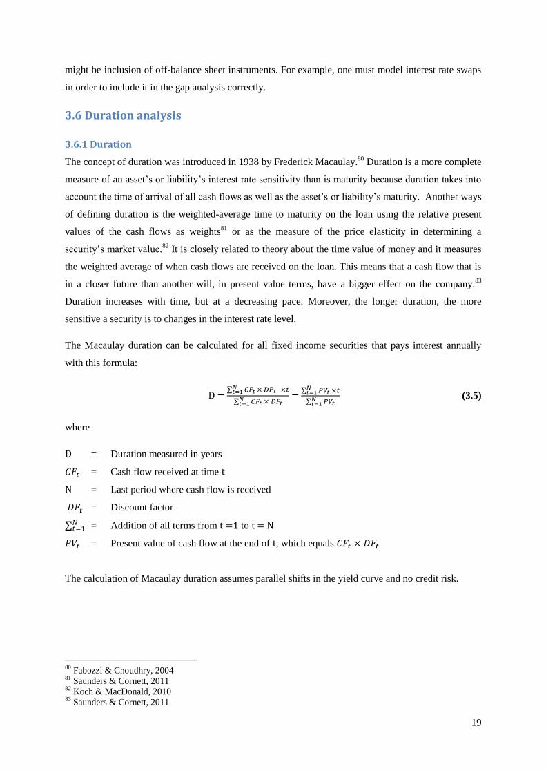
The Macaulay duration can be calculated for all fixed income securities that pays interest annually

with this formula:

D =

=

(3.5)

where

D = Duration measured in years

= Cash flow received at time t

N = Last period where cash flow is received

= Discount factor

= Addition of all terms from t =1 to t = N

= Present value of cash flow at the end of t, which equals

The calculation of Macaulay duration assumes parallel shifts in the yield curve and no credit risk.

80

Fabozzi & Choudhry, 2004 81




20

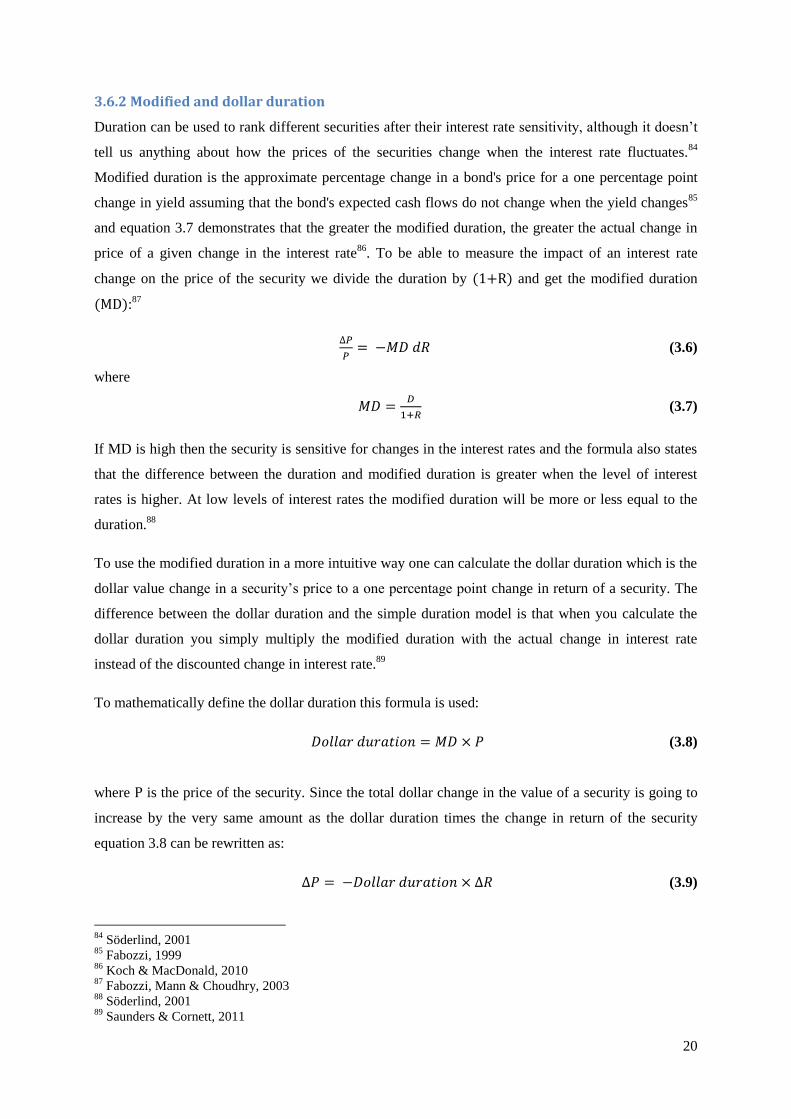
3.6.2 Modified and dollar duration

Duration can be used to rank different securities after their interest rate sensitivity, although it doesn’t

tell us anything about how the prices of the securities change when the interest rate fluctuates.84

Modified duration is the approximate percentage change in a bond's price for a one percentage point

change in yield assuming that the bond's expected cash flows do not change when the yield changes85

and equation 3.7 demonstrates that the greater the modified duration, the greater the actual change in

price of a given change in the interest rate86

. To be able to measure the impact of an interest rate

change on the price of the security we divide the duration by (1+R) and get the modified duration

(MD):87

(3.6)

where

(3.7)

If MD is high then the security is sensitive for changes in the interest rates and the formula also states

that the difference between the duration and modified duration is greater when the level of interest

rates is higher. At low levels of interest rates the modified duration will be more or less equal to the

duration.88

To use the modified duration in a more intuitive way one can calculate the dollar duration which is the

dollar value change in a security’s price to a one percentage point change in return of a security. The

difference between the dollar duration and the simple duration model is that when you calculate the

dollar duration you simply multiply the modified duration with the actual change in interest rate

instead of the discounted change in interest rate.89

To mathematically define the dollar duration this formula is used:

(3.8)

where P is the price of the security. Since the total dollar change in the value of a security is going to

increase by the very same amount as the dollar duration times the change in return of the security

equation 3.8 can be rewritten as:

(3.9)

84

Söderlind, 2001 85

Fabozzi, 1999 86


Fabozzi, Mann & Choudhry, 2003 88

Söderlind, 2001 89


21

The nature of the modified duration and the dollar duration make them well applicable for stress

testing. The duration model assumes parallel shifts in the yield curve, and by assuming for example a

one percent shift when using the dollar duration of a portfolio, this provides us with the information on

what will happen to the market value of the portfolio as the interest rate level changes.

3.6.3 Duration gap

Saunders and Cornett’s explains duration gap as “a measure of overall interest rate risk exposure of a

financial institution”. To be able to estimate the duration gap of the balance sheet, the first thing that

has to be done is to determine the duration of the asset (A) portfolio and the liability (L + E) portfolio

which can be calculated as:

and

Since the balance sheet of financial institutions only contains financial assets and liabilities a change

in the interest rates will affect the financial institution’s equity (E). This change is equal to the

difference between the change in market values of assets and liabilities on both sides of the balance

sheet.

To see how a change in A and L affects E one must determine how changes in A and L are related to

duration and to do this the following formulas are used:

and

where

and

are the percentage change in the market values of assets and liabilities, and are the

duration of assets and liabilities and

the shock to interest rates.

To show the monetary changes in assets and liabilities these equations can be rewritten as:

(3.10)

and

(3.11)

22

Rearranging and combining equation 3.10 and 3.11 with gives us the duration gap:

(3.12)

where

is a measure of the leverage of the financial institution, is the leverage

adjusted duration gap which measures the degree of duration mismatch on the balance sheet, A is the

size of the company’s assets and

is again the size of the interest rate shock.

The duration gap can be used as a benchmark for measuring how exposed a financial institution is to

fluctuations in the interest rate. A positive gap indicates that a company’s assets, on average, are more

price sensitive than the liabilities. A negative gap indicates that the weighted liabilities are more

sensitive than the weighted assets.90

What the equation suggests is that if the leverage adjusted

duration gap is zero the change in equity (because of a change in the interest rate) will be zero when

there is a change in the interest rate level.91

The manager can also change the leverage, k, instead of changing or . There are three ways to

reduce the leverage adjusted duration gap to zero. One can either reduce or increase until it equals

. Another way to reduce the gap is to reduce and increase (if we assume a positive gap) and

keep k constant. The third way is to change k and and keep constant. Reducing the gap to zero is

called immunization. An immunized security or portfolio is one in which the gain (loss) from the

higher reinvestment rate is just offset by the capital loss (gain).92

A central financial question for all companies is the mix between equity and debt, i.e. the E/A ratio.

Banks need to keep a certain level of capital adequacy due to regulations such as Basel III, whereas

non-financial companies usually can have higher leverage. In order to keep the level of equity at a

certain level, the impact of the duration gap must be controlled so that equity does not become less

than the required level. For banks, where regulation often focuses on the capital adequacy ratio (E/A),

equation 3.13 can be set to a target or minimum level in order to solve for the leverage adjusted

duration gap or external interest rate shocks. Instead of setting the target to , the bank can set

. As Saunders & Cornett state, this means that an immunizing company either can satisfy

the stockholders (E) or the regulators (E/A), but not both simultaneously. Instead of setting

, set

(3.13)

90


Kaufman, 1984 92

Koch & MacDonald, 2010

23

i.e. the leverage effect drops out, to immunize the capital adequacy ratio. 93

3.6.4 Disadvantages with the duration model

Critics mean that there are several problems with applying the duration model in practice. According

to some of them, using the duration model to lower the interest rate risk exposure by restructuring the

balance sheet is expensive and time-consuming. However, Saunders & Cornett states that this might

be true historically but because of the growth of markets for loan sales and asset securization this

might not be the case today.94

Another problem is when using an immunization strategy based on duration since the duration changes

with time. Since this is a dynamic strategy the costs of rebalancing the portfolio to maintain fully

duration matched may be high.95

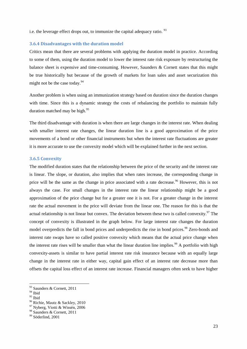
The third disadvantage with duration is when there are large changes in the interest rate. When dealing

with smaller interest rate changes, the linear duration line is a good approximation of the price

movements of a bond or other financial instruments but when the interest rate fluctuations are greater

it is more accurate to use the convexity model which will be explained further in the next section.

3.6.5 Convexity

The modified duration states that the relationship between the price of the security and the interest rate

is linear. The slope, or duration, also implies that when rates increase, the corresponding change in

price will be the same as the change in price associated with a rate decrease.96

However, this is not

always the case. For small changes in the interest rate the linear relationship might be a good

approximation of the price change but for a greater one it is not. For a greater change in the interest

rate the actual movement in the price will deviate from the linear one. The reason for this is that the

actual relationship is not linear but convex. The deviation between these two is called convexity.97

The

concept of convexity is illustrated in the graph below. For large interest rate changes the duration

model overpredicts the fall in bond prices and underpredicts the rise in bond prices.98

Zero-bonds and

interest rate swaps have so called positive convexity which means that the actual price change when

the interest rate rises will be smaller than what the linear duration line implies.99

A portfolio with high

convexity-assets is similar to have partial interest rate risk insurance because with an equally large

change in the interest rate in either way, capital gain effect of an interest rate decrease more than

offsets the capital loss effect of an interest rate increase. Financial managers often seek to have higher

93


Ibid 95

Ibid 96

Richie, Mautz & Sackley, 2010 97

Nyberg, Viotti & Wissén, 2006 98


Söderlind, 2001

24

convexity on their assets than on their liabilities because this makes them gain from both falling and

rising interest rates.100

Generally, the longer maturity on a security the higher is its convexity.101

To predict the change in the price of a security when the interest rate changes one should use the

following formula which is derived from a Taylor expansion:

(3.14)

where the first term in the simple duration model that over- or understates price changes for large

fluctuations in the interest rate. The second term is the second-order effect of an interest rate change,

the convexity adjustment. MD is still the modified duration and

and show that the convexity

effect is a second-order effect of interest rate changes while duration is a first-order effect. CX is the

parameter that reflects the degree of curvature in the price-yield curve at the current yield level which

is the point where the capital gain effect exceeds the capital loss effect for an equal change in yields in

either way. To try to measure CX one can use the following formula:

(3.15)

The sum of the terms in the brackets shows the degree to which the capital gain effect is larger than

the capital loss effect if the interest rate changes one basis-point up or down. The scaling factor

normalizes this measure to account for a larger one percentage point change in the interest rates and is

100

Kuo, 1995 101


P*

Y*

Bond price

Yield

Duration relationship

Actual relationship

Figure 3. The relationship between duration and convexity

25

used to simplify the calculations. Since one percentage point change in the interest rate is considered

to be a large effect one must take the convexity effect into account.

A commonly used scaling factor is because it is consistent with the effect of a one percentage

point change in the interest rate. Based on equation 3.9, the following equation shows how we can

measure the parameter CX:

(3.16)

The value of CX can be put into equation 3.16 and then one can assume a large rise in the interest rate

from X to Y. The formula will show that the fall in price of the security, as an effect from the rise in

the interest rate, will be smaller than what the simple duration model would suggest.102

As for duration, the convexity for an entire portfolio is the weighted convexity of each asset. Since

convexity is a desirable attribute on assets, the goal is to maximize the convexity difference between

the assets and liabilities. The convexity gap can be defined as:

(3.17)

where is the weighted convexity on the assets, and the weighted convexity of the liabilities.

When choosing between different strategies with the same duration, the one with the highest convexity

is the most preferable.

Convexity strategies – Barbell and Bullet

To obtain a great amount of convexity a financial institution manager could make use of the Barbell

strategy which means buying financial instruments with short and long duration while selling

instruments with intermediate duration. The Barbell strategy suggests that the financial manager

should buy instruments with short and long duration to the point where the weighted duration equals

the duration of the intermediate instrument. The counterpart of this strategy is a manager who is using

the Bullet strategy which means selling short and long duration instruments and buying intermediate

duration instruments. The two managers are now holding two portfolios with the same duration but

with different attributes. As mentioned above the Barbell strategy is a high convexity strategy while

the Bullet strategy is a low convexity strategy. However, in order to benefit from the higher convexity

the Barbell strategy offers a lower yield to maturity than the Bullet. This spread in yield is often

referred to as “cost of convexity”. 103

102


Fabozzi, Mann & Choudhry, 2003

26

3.7 Interest rate swaps

As mentioned in the introduction chapter, the market for interest rate swaps has grown substantially

the last decades, and is now an important instrument used by many companies in managing interest

rate risk.104

As Bodnar and von Gerich & Karjalainen state, interest rate swaps is the most commonly

used instrument to hedge interest rate risk used by non-financial companies.105

An interest rate swap is a contract between two counterparties to exchange fixed interest payments for

floating interest payments based on a notional amount over a given time period, on specific periodic

settlement dates. One of the parties takes the role as the ‘buyer’, who pays fixed interest and receives

floating interest. Conversely, the ‘seller’ pays floating interest and receives fixed interest. 106

Interest rate swaps are being traded OTC, usually with a bank acting as an intermediary between the

two counterparties.

3.7.1 Duration of different derivatives

When defining the duration of an interest rate swap, a new duration concept has to be introduced:

negative duration. In the case of falling interest rates it is the fixed rate-payer (the buyer of the swap)

who is experiencing negative duration and the fixed rate-receiver (the seller of the swap) will

experience a positive duration. The reason for this is that the buyer of the swap is paying a fixed rate

to the seller while the seller pays the buyer a floating rate. Although, if the interest rates were to rise

the seller would experience negative duration because he would still receive a fixed amount from the

buyer but would have to pay a greater amount due to the rise in interest rates.107

To calculate the duration of a swap one must divide the swap payments into two separate legs, the

floating and the fixed, and measure the duration in the same way as measuring the duration of bonds.

The following formula denotes the duration of a Pay-Fixed swap:

=

(3.18)

and for a receive-fixed swap:

=

(3.19)

104


Bodnar, 1995, von Gerich & Karjalainen, 2006 106


Smith & Smith, 2011

27

where c is the coupon rate and N is the number of periods to maturity as of the beginning of the

period.108

To calculate the duration for a cross-currency swap the general rule is to separate the cash flows into

domestic yield and foreign yield and measure the duration separately. The same principle can be

applied to FX Forwards where the two future cash flows should be divided into domestic currency

cash flow and foreign currency cash flow. 109

To calculate the dollar duration of a swap or other derivative, the same principle is applied. Thus, the

dollar duration of a swap is110

:

and

–

3.8 Stress testing

According to Bank of International Settlements (BIS) a financial institution should subject its asset

and liability portfolio to different kinds of stress tests. These tests should provide information about

the risk level of the financial institution and expose where it is most vulnerable. Since different

institutions have different characteristics, these tests should be tailor made in order to best fit the

institution.111

The most common techniques for stress testing a portfolio are to assume either a change

in one factor (sensitivity analysis) or a change in two or more factors (scenario analysis). 112

BIS names a couple of ways to stress test a financial institutions and one of these includes a change

the general level of interest rates by assume a parallel shift of the yield curve. A stress test should also

take under consideration the liquidity of the positions under stressful situations and consider a worst

case scenario in addition to more probable events. 113

Stress testing provides a full valuation approach to assess interest rate risk of a bond or portfolio. The

most widely used stress tests when measuring interest rate risk is to assume a parallel shift of the yield

curve or a change of the slope of the yield curve. A commonly used scenario required by financial

108

Smith & Smith, 2011 109

Ibid 110

Buetow & Fabozzi, 2001 111



Bank for International Settlements, 2004

28

authorities is a parallel shift of ±1 percentage point of the yield curve. Since the value of any financial

instrument must be the value of its future cash flows discounted with yield curve, what a stress test

suggests is a change in the yield (r) used for discounting in the formula below, resulting in a change in

the market value of the security:

Although stress testing is an effective and intuitive way of measuring interest rate risk firms should not

make decisions about their risk management policies solely based on their stress test but should be

incorporating other quantitative and qualitative methods.114

Just like most theories and methods even stress testing have its disadvantages. Like described, a stress

test estimates the exposure to a specific event but it does not say anything about the probability of such

an event occurring. It is also time consuming to conduct a stress test if the portfolio has a large amount

of positions and contains complex instruments, and it may also require data from different business

units. Third, it might be difficult for the financial risk manager to choose which scenarios that should

be tested and how to interpret the results in an efficient way.115

116

3.9 Other types of interest rate risk measures

This section captures some other interest rate measures being used.

3.9.1 Maturity

The time to maturity, or the number of years remaining prior to the final principal payment, can be a

resourceful measure of interest rate risk. All other factors held constant, the longer the maturity of a

bond, the greater the volatility in market value due to a change in interest rates.117

The maturity of a

portfolio is simply the weighted maturity of all bonds or securities, which makes it possible to

calculate the maturity for total assets as well as total liabilities. The gap between the maturity of assets

and liabilities indicates that the company might be affected by refinancing risk, as being described in

section 3.3.2.1. However, maturity as a measure of interest rate risk does not take into account the

timing of cash flows within the security’s maturity time span.

3.9.2 Fixed-to-floating ratio

The fixed-to-floating ratio is a measure of the debt paying a fixed cash flow in relation to the total

debt, including loans with floating interest payments.118

The idea with the fixed-to-floating ratio is to

114


Ibid 116

Söderlind, 2001 117

Fabozzi, 2007 118

Von Gerich & Karjalainen, 2006

29

monitor the proportion of fixed and floating payments, in order to be able to balance the exposure to

different rates. It can be used to setting a goal level of fixed versus floating interest rate payments. A

high proportion of fixed rate debt causes a risk exposure if interest rates fall.119

Conversely, a high

proportion of floating rate debt creates an exposure if the interest rates rise.

3.9.3 Value at Risk

Value at Risk (VaR) is a statistical measurement and predicts the maximum possible loss given a

certain scenario by using probability distributions. This can be done in two ways, either by considering

the actual distribution or by approximating the distribution by a parametric approximation such as a

normal distribution. Normally, the confidence level is 95 percent.120

119

Buckley, 2004 120

Jorion, 2001

30

4 Emipirical data & analysis

This chapter will begin with a short introduction to the case company. This will be followed by the

results of the survey conducted. Last, empirical data and practical calculations of the theoretical

framework will be presented and applied on TIFI’s portfolio. Moreover, an analysis on the portfolio

from the perspective of the different theories will be made

4.1 Toyota Industries Finance International AB

Toyota Material Handling Group (TMHG), which belongs to its parent company Toyota Industries

Corporation (TICO), is the biggest forklift manufacturer of the world. In 2000 they acquired the

Swedish forklift manufacturer BT located in Mjölby, Sweden, and today this is where the headquarters

of Toyota Material Handling Europe (TMHE) is located.

Toyota Industries Finance International AB (TIFI) is established to provide financial and treasury

services within the whole of TICO group outside Japan.121

The responsibilities of TIFI is among many things to function as a in house bank that deals with credit

management and funding risk control as well as cash operations management. It also deals with

accounting, treasury development and other corporate services.

Each company within the TICO group should as a rule finance its operations with loans from TIFI

with a maturity structure that corresponds to the normal maturity structure of the assets financed. This

means that all financing needed within the TMHE group have to go through TIFI in Mjölby. The

board has given TIFI mandate to use derivative to hedge its interest risk and have stated some rules

about how to hedge its assets and liabilities:

Assets and liabilities over one year should be basically hedged.

Maximum duration gap between asset and liability shorter than one year is set within 3

months.

4.2 Other treasury departments of international industrial company groups

The responding treasury departments are the ones of SCA, Sandvik, Trelleborg, Volvo, Atlas Copco,

Alfa Laval and two other industrial companies which have chosen to be anonymous.

The kinds of interest rate risk measurement methods used by the companies differ from one another.

The methods being used are mainly duration- and maturity- and Value at Risk models and different

kinds of stress tests. Most companies answer that they have to follow certain regulations set by the

management. These regulations regard the exposure to different time buckets or currencies. To

quantify the measurements most companies seem to assume a parallel one percentage point shift of the

121

Toyota Industries Finance International, 2010

31

yield curve and one company assumes a “worst case scenario” where all market interest rates moves in

a unfavorable direction.

According to the respondents of the interviewed treasury managers of the main reasons for choosing a

specific method of measuring interest rate risk is the simplicity since it is important that it is explicable

to the management team that might not be familiar with financial economics. Another reason is that a

more advanced method might not be needed since most treasury departments of large industrial

company group’s don’t take speculative positions on the financial market to make money from it.

“An industrial company’s treasury department normally focuses on minimizing the financial risks to

support the core business which in Trelleborg’s case is to deliver and develop high performing

solutions that seal, dampen and protect in challenging industrial environments.”122

4.3 The empirical approach

To be able to back-test TIFI’s portfolio we have chosen five different dates during the last five years

when the volatility in interest rate market have been the highest. TIFI’s portfolio consists of hundreds

of financial positions, including different kinds of loans, interest rate swaps, cross currency interest

rate swaps and foreign exchange forwards in several currencies. Because of the vast amount of data,

the modeling and the calculations become a complex and time consuming task. We have calculated the

portfolio’s value the day before the interest rate shock to see how the change in interest rates affected

it. The dates that have been chosen and the corresponding change in interest rates are presented below.

122

Apelgren, 2012

32

Table 2. Interest rate shocks

Date Percentage change

2008-10-23 - 0.4125

2008-12-03 - 0.2325

2008-12-04 - 1.17

2009-04-17 - 0.055

2009-07-02 - 0.215

The change of the term structure between the days can be illustrated in a graph. The black graph

illustrates the first day, and the grey line illustrates the day of the interest rate shock.

Figure 4. Interest rate shocks

2008-10-22-23 2008-12-02-03 2008-12-03-04

2009-04-16-17 2009-07-01-02

The five methods of measuring interest rate risk presented in chapter 3 will here be applied, compared

and eventually evaluated.

To be able to do the necessary calculations the cash flows of all off balance sheet assets and liabilities,

such as FX forwards, interest rate swaps and cross interest rate swaps, should be divided into a pay

side and a receive side. After this it is possible to calculate the interest rate risk.

33

4.4 Repricing model

By obtaining the book values of the financial positions, as well as modeling off balance sheet

instruments, it is possible to perform a repricing analysis. The authors have chosen not to include the

cash pool in the analysis because of the following reasons:

The cash pool could either be placed in the one day time bucket since it is very liquid and the

interest on the cash pool is being calculated on a daily basis. However, placing the cash pool

in the one day time bucket would over exaggerate the risk on a one day time horizon, making

it seems like the risk was very high.

The other alternative would be to divide the cash pool and placing it into different time

buckets. However, the nature of the cash pool makes this method hard to make use of

practically, and would wrongfully predict the risk.

Given that these two methods will not provide a good quantification of the risk exposure, the

cash pool will be excluded from the repricing analysis. Further, since the cash pool is not at all

rate sensitive in the same way as other securities, this also makes a good reason for it to be

excluded.

After putting rate sensitive assets and liabilities in their respective time buckets, it is possible to

calculate the gap from equation 3.1. The gap represents TIFI’s net interest rate risk exposure. The

cumulative gap is the summarized gaps from all time periods, using equation 3.3. The change in net

interest income is calculated from equation 3.2, which provides us with information about how a one

percentage point change in the interest rate level would affect the net interest income. Last, the gap

ratio is calculated from equation 3.4, which is a measure of risk exposure.

Table 3. Repricing analysis of 2008-10-22

Time period RSA RSL Gap Cumulative gap ΔNII (1%) ΔNII (-1%) Gap ratio

1. 1 day 62 001 322 124 399 833 -62 398 511 -62 398 511 -623 985 623 985 -0,4%

2. 1 day - 3 months 8 785 435 099 6 267 175 779 2 518 259 320 2 455 860 809 25 182 593 -25 182 593 15,6%

3. 3 - 6 months 3 686 269 955 4 162 557 865 -476 287 910 1 979 572 899 -4 762 879 4 762 879 -3,0%

4. 6 - 12 months 99 138 299 11 622 058 87 516 241 2 067 089 141 875 162 -875 162 0,5%

5. 1 - 5 years 3 511 950 216 3 617 204 240 -105 254 023 1 961 835 117 -1 052 540 1 052 540 -0,7%

6. > 5 years 0 0 0 1 961 835 117 0 0 0,0%

Total 16 144 794 891 14 182 959 774 1 961 835 117 1 961 835 117 19 618 351 -19 618 351 12,2%

34





1. 1 day 65 300 212 99 744 434 -34 444 222 -34 444 222 -344 442 344 442 -0,1%

2. 2 days - 3 months 11 197 488 884 7 626 478 395 3 571 010 489 3 536 566 266 35 710 105 -35 710 105 13,3%

3. 3 - 6 months 408 181 017 764 603 036 -356 422 019 3 180 144 247 -3 564 220 3 564 220 12,0%

4. 6 - 12 months 1 220 925 742 1 694 114 900 -473 189 158 2 706 955 089 -4 731 892 4 731 892 10,2%

5. 1 - 5 years 2 562 471 197 2 565 716 717 -3 245 520 2 703 709 570 -32 455 32 455 10,2%

6. > 5 years 11 096 430 250 7 633 626 189 3 462 804 061 6 166 513 631 34 628 041 -34 628 041 23,2%

Total 26 550 797 301 20 384 283 670 6 166 513 631 6 166 513 631 61 665 136 -61 665 136 23,2%



1. 1 day 10 703 323 10 695 000 8 323 8 323 83 -83 0,0%

2. 2 days - 3 months 9 834 226 615 6 012 498 424 3 821 728 192 3 821 736 515 38 217 282 -38 217 282 27,1%

3. 3 - 6 months 478 334 780 1 182 768 758 -704 433 978 3 117 302 537 -7 044 340 7 044 340 22,1%

4. 6 - 12 months 98 602 825 684 484 328 -585 881 504 2 531 421 033 -5 858 815 5 858 815 17,9%

5. 1 - 5 years 3 700 758 724 4 022 797 525 -322 038 801 2 209 382 232 -3 220 388 3 220 388 15,6%

6. > 5 years 0 0 0 2 209 382 232 0 0 15,6%

Total 14 122 626 267 11 913 244 035 2 209 382 232 2 209 382 232 22 093 822 -22 093 822 15,6%


1. 1 day 718 428 039 381 961 826 336 466 213 336 466 213 3 364 662 -3 364 662 1,7%

2. 2 days - 3 months 12 067 232 225 9 890 160 130 2 177 072 095 2 513 538 308 21 770 721 -21 770 721 10,7%

3. 3 - 6 months 3 545 914 555 4 122 891 331 -576 976 776 1 936 561 532 -5 769 768 5 769 768 -2,8%

4. 6 - 12 months 242 658 399 27 861 056 214 797 343 2 151 358 875 2 147 973 -2 147 973 1,1%

5. 1 - 5 years 3 698 579 195 4 161 950 341 -463 371 147 1 687 987 728 -4 633 711 4 633 711 -2,3%

6. > 5 years 0 0 0 1 687 987 728 0 0 0,0%

Total 20 272 812 413 18 584 824 684 1 687 987 728 1 687 987 728 16 879 877 -16 879 877 8,3%


1. 1 day 300 000 000 0 300 000 000 300 000 000 3 000 000 -3 000 000 1,5%

2. 2 days - 3 months 12 419 560 554 10 050 540 660 2 369 019 894 2 669 019 894 23 690 199 -23 690 199 11,8%

3. 3 - 6 months 3 442 479 100 4 029 775 673 -587 296 574 2 081 723 321 -5 872 966 5 872 966 -2,9%

4. 6 - 12 months 230 154 885 27 788 445 202 366 441 2 284 089 761 2 023 664 -2 023 664 1,0%

5. 1 - 5 years 3 720 691 238 4 197 438 851 -476 747 613 1 807 342 148 -4 767 476 4 767 476 -2,4%

6. > 5 years 0

0 1 807 342 148 0 0 0,0%

Total 20 112 885 777 18 305 543 629 1 807 342 148 1 807 342 148 18 073 421 -18 073 421 9,0%

35

The above five dates show a repricing model approach to quantification of the interest rate risk the day

before significant interest rate movements. A general conclusion of these results is that TIFI has a

significant interest rate risk exposure in the second time period, which is 2 days – 3 months. This is

both being seen as a gap, and also as an effect in the change of net interest income (ΔNII), and as a

large proportion of total assets, i.e. the gap ratio. TIFI generally has a positive gap in this time period,

which means that a fall of the interest rates will have a negative effect on the company’s cash flows.

4.5 Duration

To correctly measure the duration of the portfolio the cash pool have been included in the calculations.

To make sure that only the market value change of the different positions has affected the portfolio

value between the day before the interest rate shock and the day of it, the authors have only taken into

account the positions that do exist on both days. This means that positions that have expired on the day

before the shock have been deleted. In addition, adjustments concerning the fluctuation of exchange

rates between the two days and its effect on the market values have been made. The reason for this is

that only the direct effect of the interest rate change should be measured. To do that, the interest rate

change was isolated by assuming that the exchange rate has been the same on both days.

The duration from the day before the shock predicts a gain or loss from a change in the interest rate.

Therefore, it is interesting to see the actual outcome from an interest rate change since it will show

how well the duration analysis predicted the change in market value of the portfolio. The size of the

discrepancy between the result suggested by the duration and the actual outcome will help us

determine whether the duration analysis is a good measurement of interest rate risk for TIFI.

For some of the measures, an interest rate change must be assumed. The obvious problem with these

measures is what interest rate change to assume, since it is difficult to predict these changes. As a base

for the discussion in chapter 5, two different interest rate shocks were tested. First, a one percentage

point fall in the interest rate level has been assumed. Second, the actual change in LIBOR has been

used for the same reasons mentioned in section 2.4. What the calculations shows is that the LIBOR is

not a good benchmark rate for TIFI. Another alternative for the back testing would be to calculate the

implied interest rate change, and use this in the models. However, this would always make the

measures seem perfectly “correct”, and it is not practically possible to foresee the interest rate shock.

To calculate the following measures, the formulas in section 3.5 were used. DA and DL represent the

simple Macaulay duration of assets and liabilities from equation 3.5. ΔE is the duration gap calculated

using equation 3.12. MDA and MDL are the modified duration (equation 3.7). From this ΔP was

calculated from equation 3.6, which represents the impact on the portfolio value from a given change

in the interest rate level. Then, the convexity of the assets and the liabilities were calculated using

36

equation 3.15. Using this result, the convexity gap could be calculated with equation 3.17. From

equation 3.14, the effect of the convexity gap of the portfolio could be calculated. Last, the dollar

duration was calculated using equation 3.8 and the change in market values due to this with equation

3.9.

2008-10-22

Table 8. Duration analysis of 2008-10-22

- 1 % LIBOR change (- 0.4125 %)

DA 0.53

DL 0.62

ΔE - 4 413 705 SEK - 1 820 653 SEK

MDA 0.53

MDL 0.61

ΔP - 4 370 005 SEK - 1 802 627 SEK

CX gap -0.16

CX effect - 29 790 SEK - 5 069 SEK

Dollar duration -456 885 991 SEK

ΔP - 4 568 860 SEK - 1 884 654 SEK

2008-10-23

ΔP: - 6 001 979 kr

Implicit change in interest rate level: - 1.4 %

As can be seen in the table above, on the 22th of October 2008 TIFI’s liabilities have longer duration

than the assets which means that liabilities are more sensitive to interest rate changes. The weighted

portfolio duration is 0.63 and the modified duration for the assets and liabilities are 0.53 and 0.61

respectively. The assumed interest rate fall of one percent and the actual interest rate fall of 0.4125

percent on the 23th of October present different outcomes in terms of a loss due to the interest rate

change. The suggested loss from the assumed one percentage point fall is approximately 4.4 million

SEK and the actual fall of 0.4125 percent suggests a loss of approximately 1.8 million SEK.

However, the actual loss in terms of a decrease in the market value of the positions was 6 million SEK

which implies an interest rate fall of 1.4 percentage points.

37


- 1 % LIBOR change (-0.2325 %)

DA 0.46

DL 0.57

ΔE -16 644 815 SEK -3 711 174 SEK

MDA 0.46

MDL 0.57

ΔP - 16 480 015 SEK - 3 872 076 SEK

CX gap - 0.16


Dollar duration -1 665 408 915 SEK

ΔP - 16 654 089 SEK - 3 872 076 SEK

2008-12-03

ΔP: - 20 257 691 SEK

Implicit interest rate change: - 1.2 %

On the third of December the interest rate dropped 0.2325 percent. The duration calculations on the

day before would suggest a loss of 3.7 million SEK from such a drop and the assumed fall of one

percent would imply a loss of 16.4 million SEK. However, the actual gain from the interest rate fall

was approximately 20 million SEK and the implied interest rate change was a rise with almost only

0.09 percentage points.


- 1 % LIBOR change (- 1.17 %)

DA 0.47

DL 0.58

ΔE -16 903 057 SEK - 19 776 577 SEK

MDA 0.47

MDL 0.58

ΔP - 16 735 700 SEK - 19 580 769 SEK

CX gap - 0.16

CX effect - 92 800 - 127 034 SEK

Dollar duration -1 690 916 758 SEK

ΔP -16 909 168 SEK - 19 783 726 SEK

38

2008-12-04

ΔP: + 1 526 023 SEK

Implicit interest rate change: + 0.09 %

On the 4th of December the actual drop in interest rate was 1.17 % which would have suggested a loss

of 17 million SEK. The actual outcome was a gain of approximately 1.5 million which in turn implied

an interest rate rise of 0.09 percentage points.


- 1 % LIBOR change (- 0.055 %)

DA 0.59

DL 0.74

ΔE -9 590 798 SEK - 527 494 SEK

MDA 0.58

MDL 0.73

ΔP - 9 495 839 SEK - 522 271 SEK

CX gap - 0.50

CX effect - 193 100 SEK - 584 SEK

Dollar duration - 957 133 720 SEK

ΔP - 9 571 337 SEK - 526 424 SEK

2009-04-17

ΔP: - 33 571 SEK


When the interest rate level fell with 0.055 % on the 17th of April 2009 the duration calculations

predicted a loss of 476 797 SEK but the actual outcome was a loss of 33 571 SEK and a implied rise

of the interest rate level with 0.004 percentage points.

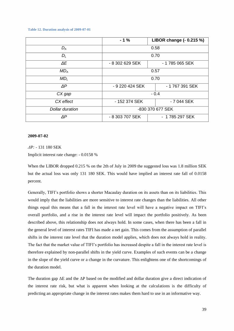
39


- 1 % LIBOR change (- 0.215 %)

DA 0.58

DL 0.70

ΔE - 8 302 629 SEK - 1 785 065 SEK

MDA 0.57

MDL 0.70

ΔP - 9 220 424 SEK - 1 767 391 SEK

CX gap - 0.4


Dollar duration -830 370 677 SEK

ΔP - 8 303 707 SEK - 1 785 297 SEK

2009-07-02

ΔP: - 131 180 SEK


When the LIBOR dropped 0.215 % on the 2th of July in 2009 the suggested loss was 1.8 million SEK

but the actual loss was only 131 180 SEK. This would have implied an interest rate fall of 0.0158

percent.

Generally, TIFI’s portfolio shows a shorter Macaulay duration on its assets than on its liabilities. This

would imply that the liabilities are more sensitive to interest rate changes than the liabilities. All other

things equal this means that a fall in the interest rate level will have a negative impact on TIFI’s

overall portfolio, and a rise in the interest rate level will impact the portfolio positively. As been

described above, this relationship does not always hold. In some cases, when there has been a fall in

the general level of interest rates TIFI has made a net gain. This comes from the assumption of parallel

shifts in the interest rate level that the duration model applies, which does not always hold in reality.

The fact that the market value of TIFI’s portfolio has increased despite a fall in the interest rate level is

therefore explained by non-parallel shifts in the yield curve. Examples of such events can be a change

in the slope of the yield curve or a change in the curvature. This enlightens one of the shortcomings of

the duration model.

The duration gap ΔE and the ΔP based on the modified and dollar duration give a direct indication of

the interest rate risk, but what is apparent when looking at the calculations is the difficulty of

predicting an appropriate change in the interest rates makes them hard to use in an informative way.

40

Using equation 3.7, TIFI’s portfolio shows relatively low modified duration, which indicates little

exposure to interest rate risk. The suggested percentage change in market value of the overall portfolio

increases when incorporating convexity into the calculation. This comes from the fact that the

convexity of TIFI’s portfolio is negative. TIFI’s portfolio shows negative convexity in all different

scenarios, which is undesirable. The convexity strategies described in section 3.6.5.1 would benefit the

portfolio positively.

4.6 Stress test

By assuming a parallel shift in the interest rate level, it is possible to measure the interest rate

sensitivity of the portfolio. Table 13 shows that TIFI’s portfolio would benefit from a fall in interest

rates and that a positive interest rate change would have a negative impact on the portfolio.

Table 13. Stress test

Dates IR Down 1% IR Up 1%

2008-10-22 - 5 032 228 + 4 153 819

2008-12-02 - 16 752 089 + 16 264 065

2008-12-03 - 17 105 488 + 16 264 065

2009-04-16 - 8 646 471 + 8 245 789

2009-07-01 - 8 471 669 + 8 143 665

As can be seen, TIFI’s portfolio generally looses more from a fall in the interest rate level, than it

gains from a rise. This attribute is also confirmed by the negative convexity from the duration analysis.

4.7 Maturity

Table 14. Maturity profile

Date Assets Liabilities Maturity gap

2008-10-22 0.81 0.92 -0.11

2008-12-02 0.67 0.79 -0.12

2008-12-03 0.68 0.80 -0.13

2009-04-16 0.87 1.09 -0.22

2009-07-01 0.85 1.02 -0.17

The table above shows the maturity structure of the both assets and liabilities and the gap between

them. As can be seen the maturity gap is consistently negative which states that the assets matures

sooner than the liabilities. If one assumes a fall in the interest rate during the period when assets have

41

matured and the liabilities have not TIFI will have to reinvest at an interest rate level that is lower than

the cost of their debt.

4.8 Fixed-to-floating ratio

Table 15. Fixed-to-floating ratio

Date Fixed/floating ratio

2008-10-22 97 %

2008-12-02 98 %

2008-12-03 98 %

2009-04-16 96 %

2009-07-01 87 %

Table 15 shows that TIFI’s amount of fixed debt has been greater than its amount of floating which

suggests that it have been more exposed to negative interest rate shocks. Ernst & Young’s report about

treasury departments states that a majority of companies have a fixed/floating ratio within the interval

of 40 – 80 %.123

TIFI’s fixed/floating ratio range from 87% to 97 % and this makes them more

vulnerable to a fall in the interest rate level. However, a ratio close to one means that the company

isn’t exposed to interest rate risk if it holds the positions to maturity. But they might still find

themselves having to borrow at a higher interest rate when renewing an expired position. This

observation is also confirmed by the results from the other measurement methods such as the duration

analysis.

123

Clarke & Teague, 2005

42

5 Discussion

This chapter will evaluate and compare the different measures, and discuss the weaknesses and

advantages as well as draw conclusions supported by the survey results. The chapter will begin

discussing the measurement of interest rate risk in treasury departments of other industrial company

groups, and then discuss the differences between treasury departments and commercial banks in terms

of interest rate risk. Finally, duration analysis, stress testing, the repricing model, maturity and fixed-

to-floating will be discussed.

5.1 Measurement of interest rate risk in treasury departments of other

industrial company groups As stated in section 4.2 there are a variety of measurement methods being used. One of the reasons for

this is probably that different treasury software focuses on different methods and that the employees of

the treasury departments have different skills. One can assume that treasury departments that have

managers who have been schooled in the commercial banking sector might use more advanced

methods.

Some of the methods used have been chosen because it is easy to communicate to the management.

One of these is the Value at Risk. Even though this gives the management a good approximation about

the worst possible loss under normal conditions one must remember that this measure does not offer a

way to calculate how the treasury department should be positioned to reduce the interest rate risk.

5.2 Differences between commercial banks and treasury departments The main difference between a commercial bank and a treasury department is their core business.

Generally, the main goal of a treasury department of an industrial company is to support the

production and selling of their industrial products by loaning money to different parts within the

company group. Since financial risk taking could potentially put the whole company at jeopardy they

are rather risk avert. Another difference is that a treasury doesn’t need to follow the same regulations

regarding the equity ratio as a commercial bank. The reasons for this are many and one of them is that

a treasury department can get financial aid from the mother company if they are experiencing losses.

Another reason is that treasury department does not deal with private customers’ money. The third

reason is that a commercial bank is more important for the economy and the financial system, which

means that the fall of a commercial bank would make more damage.

The main goal of a commercial bank is to use their capital and financial products to make money. To

be able to satisfy shareholders they often use leverage which means bigger risks. However, at the same

time they must still follow the Basel-regulations which state what ratio between capital and debt that

the bank needs. Because of the Basel regulations the banks need to make sure that their capital

adequacy ratio (E/A) do not fall below the minimum required level since this would lead to demands

from financial regulators which in turn would affect the credibility of the bank as well as the value of

43

the shares. This means that commercial banks should consider their capital adequacy ratio more than

their absolute amount of equity.

As stated, the regulations about the capital adequacy ratio do not concern treasury departments unless

the management of the mother company has their own regulations. Because of this the treasury

department could focus only on the absolute amount of equity.

In terms of interest rate risk the assumptions from above still hold. Generally, the treasury department

uses their loan portfolio as an equity hedge which means that if they lend money to a company within

the company group they also take the opposite position in the same currency in the financial market.

This makes the balance sheet immune to interest- and exchange rate fluctuations.

The main reason why a commercial bank is more exposed to interest rate risk is because of their core

business which is maximizing yield while minimizing the financial risk. A commercial bank often

lends money with long maturity while borrowing from depositors with short maturity. This makes

them very exposed to changes in the interest rate level and because of this they frequently use interest

rate derivatives to match their liabilities with their assets.

To summarize the discussion one can say that the main difference between a commercial bank and a

treasury department is that the former tries to earn money from interest rate fluctuations using

derivatives, while the latter wants to minimize the very same risk to better support the company group.

5.3 Duration The authors have shown how to make use of the duration measure in several ways. First, the Macaulay

duration of the assets and liabilities were calculated. This measure gives an indication of the interest

rate risk in terms of a time difference of the weighted cash flows. It was also shown how these

measures can be used to get a direct measure of the interest rate risk in monetary terms. The direct

measures based on the duration gap, modified duration, and dollar duration all gives a similar result.

Because of this fact, if choosing between these direct duration measures, it then comes to what method

is easier to carry out, which is a totally subjective matter. An advantage of using an indicative measure

such as the Macaulay duration is that it doesn’t require a prediction or assumption of a change in the

interest rate level. It simply gives an overall indication of the interest rate risk, no matter how the

interest rate will fluctuate. On the other hand, the direct, monetary measures gives a concrete view of

the interest rate risk exposure, and how much an assumed change in the interest rate level will impact

the company’s portfolio and equity. However, this requires a forecast of the interest rate level. This

might be difficult in reality, and when the forecast proves to be wrong, this may lead to significant

losses.

For banks with extensive trading activity, duration might be an interesting measure since it measures

change in market value. Further, implementing duration analysis is less complicated for banks

44

compared with regular companies, since the balance sheet of a bank regularly only contains financial

securities. Calculating duration on non-financial assets and liabilities can be a difficult task. Treasury

departments in general also only possess financial assets and liabilities, which simplifies the

implementation of duration analysis. However, treasury departments can be said to have less trading

activity and are therefore less concerned of changes in the market value of their securities, since they

regularly hold their positions until maturity. This would imply that it is better to measure the change in

net interest income. Still, other advantages make duration analysis well usable for treasury

departments.

The duration model is a so called parsimonious model which means it makes a number of

simplifications. This case study has shown the effects of these simplifications. For example, at a

number of occasions, the duration model clearly has understated the actual change in market value

when comparing the duration model predictions with the stress test, which is according to theory. A

correction closer to the real change in market value predicted by the stress test is being obtained by

inclusion of convexity into the calculations. The larger the change in interest level, the more important

gets convexity. This study shows that the convexity effect can have a significant impact in monetary

terms for large interest rate movements. One should also not underestimate the fact that a negative

convexity gap is a “lose-lose”-situation, i.e. the loss due to a negative convexity gap appears both

when the interest rates fall as well as when the interest rate rises. A notable result from the survey

conducted in this thesis is that the respondents do not see convexity as an important factor to consider.

This might indicate that the convexity effect is so relatively weak so that it does not pay off to

consider. This may seem contradicting and may be to the fact that this thesis shows that convexity can

have large impact in absolute terms, but relative to the whole portfolio, the convexity effect may not

be large enough to consider for a treasury department.

An advantage using the duration model to predict a change in market value instead of a stress test can

be that one does not have access to the required software in order to perform a stress test, and in that

sense, a duration based stress test can be a resourceful alternative. However, most treasury

departments today seem to use some kind of treasury management system which would enable correct

stress testing. Nevertheless, the duration model approach to stress testing has its advantages over stress

testing. Similar with Value-at-Risk, stress testing itself cannot be used to manage and control the

interest rate risk exposure. Duration on the other hand can be used by setting a goal of for example a

maximum loss of equity, and at the same time be a good approximation of the price-yield relationship.

From this, the interest rate risk can be controlled using the strategies in section 3.5.

What has become apparent during the work of this thesis is that duration requires a vast amount of

data, since it requires data of each single position. Additionally, when dealing with derivatives such as

interest rate swaps and cross currency interest rate swaps requires extra work due to correct modeling

45

in order to make it viable with duration analysis. Furthermore, as we have seen, it is not obvious how

to include securities with undefined maturity such as cash pools in the calculations. The authors’

opinion on this matter after conducting this study is however that cash pools should be treated as

having a duration of zero, since weighting over money into a cash pool reduces the interest rate risk.

Another subject that has come up when doing the calculations is that when the company lacks some

kind of benchmark to compare the measures with, the measures become much less meaningful and

useful. By having a benchmark, it is much easier to interpret the measures, and therefore easier to be

able to control the interest rate risk by setting a goal level. This is true for both treasury departments

and other companies. When a goal level has been decided it is possible to rebalance the portfolio in

order to maintain a certain level of interest rate risk. This raises the question of how often the company

should rebalance. The company must therefore evaluate the costs of rebalancing as well as how time

consuming it is. In the case study conducted in this thesis, we have seen that the portfolio can change

largely on a day-to-day basis, which would be a challenging task when rebalancing.

One further perspective on duration analysis as a tool for treasury departments is the capability of the

measure to be communicated in an understandable way to the board of directors. Is the concept of

duration understandable for people in the board with limited knowledge of financial economics? If

not, if however choosing duration as a measure for interest rate risk, one of the monetary duration

measures might be preferable since it might be easier to grasp a concrete measure. One can argue that

for example Value-at-Risk would be a more communicative measure more suitable to present for the

board of directors.

When comparing duration analysis with the repricing model, a number of crucial differences are being

noticed. The repricing model only takes into account the next repricing date or expiry date, whereas

duration analysis takes into account all future cash flows, which means it gives a more complete view

of the real situation. For practical purposes, the number of time buckets in the repricing model must be

limited. Given this, it raises the question of which time periods to use. Changing the time periods can

easily give a different picture of the company’s interest rate sensitivity. Another crucial difference

between the duration model and the repricing model is when it comes to managing the interest rate

risk. If a company wants to immunize using the repricing model, it must consider each single time

bucket and manage each one of them by taking new positions or using derivatives. When using the

duration model to manage the interest rate risk however, only one number needs to be considered and

the whole portfolio can be managed through this. Besides the practical simplicity of this, it also

reduces transaction costs in comparison with the repricing model.

5.4 Stress testing Stress tests are performed to see how the market value of the portfolio changes if the interest rate

fluctuates and are often made by assuming a parallel shift of the yield curve in both directions in all

46

relevant interest rates. The survey showed that treasury departments assume a parallel shift in one

direction and focus on the net effect of the change and then assume a shift in the other direction.

However, one of the respondents uses a so called “worst case scenario” where all the interest rates

move in an unfavorable direction which leads to what BIS call the maximum loss approach.

One of the advantages with a stress test is that it is easy to both communicate to management and

conduct since treasury software usually includes this function. The fact that it requires large amounts

of data is not, according to the authors, a problem since all deals and positions are already stored in the

treasury software for other purposes such as managing the portfolio. The stress test will present a

possible outcome in monetary terms from an interest rate shift and the board can then take decisions

about the level of the treasury departments risk exposure. One of the disadvantages with the stress test

is that it does not give the treasury departments the necessary tools for adjusting the interest rate risk;

it is simply presenting the possible outcome from a change in the interest rate risk.

The stress tests performed on TIFI’s portfolio show similar results as the stress test based on duration

analysis. This is because both stress tests assume the same parallel shift of the yield curve. Another

similarity with the duration analysis is the criteria that the balance sheet only contains financial assets

and liabilities. Since a treasury department satisfies this criterion the stress test can be used as interest

rate risk measure. Unlike the duration model the users of a stress test must have a prediction of the

future interest rate level. Even though the stress test tests both a positive and negative change of the

interest rate of an equal amount the treasury department needs to determine which one is more likely.

Predicting the future interest might be a big problem for any financial institution since there are many

different interest rates, and events affecting them, to consider. The authors do not think that treasury

departments should try to forecast the interest rates since it would be both expensive and, in a manner,

speculative since forecasts often prove to be wrong.

To be able to compare a stress test with the repricing model one must remember that the two models

measures two separate things. While the stress test provides potential loss or gain due to the change in

market value of the securities from a change in the interest rate level the repricing model shows at

which dates the portfolio is exposed to reinvesting and refinancing risks while. In the repricing model

the market value is held constant. A commercial or investment bank with substantial trading positions

might be better off using a stress test because of the nature of their business. The stress test measure

the change in market value due to a change in the interest rate level which is important for a company

which balance sheet only contains financial securities. However, even though the balance sheet of a

treasury department also contains financial assets and liabilities its core business is not to make money

from taking active positions in the market. Treasury department usually takes counter positions to

hedge, for example, a loan to another part of the company and not to earn money from the fluctuations

in the interest rate market. Since treasury departments, in general, hold their positions to the expiry

47

date the need for monitor the change in market value might not be as big as for a commercial bank. To

manage the portfolio using the repricing model the treasury department needs to use derivatives such

as interest rate swaps to immunize all different time buckets against fluctuations in the interest rate

market to have an immunized portfolio and this is both costly and time consuming.

5.5 Repricing model The repricing model is a straightforward method which is easy to communicate. When taking the point

of the required amount of data to be able to perform the analysis into consideration, the repricing

model requires approximately the same amount as the duration model. The repricing model offers

another approach to interest rate risk than duration analysis. Instead of focusing on the change in

market value, it measures the impact on net interest income. As written before, this would make the

repricing model more suitable for companies with little trading activity, such as treasury departments.

Despite this, both surveys earlier cited in this thesis such as the ones from von Gerich & Karjalainen,

Wiedemann and Ernst & Young’s Treasury Operations Survey and the survey conducted in this thesis

show a very limited use of the repricing model among treasury departments. This might be because of

several reasons, both depending on the repricing model itself, but also because of the benefits of other

methods. In this thesis we have seen how large interest rate moves causes significant changes in the

market value of a treasury department’s portfolio. Focusing only on the book value of assets and

liabilities may then seem a little naïve, since it doesn’t capture the “true” risk exposure. The empirical

section of this thesis regarding the repricing model has shown one further of the shortcomings of the

repricing model. The portfolio of the case study company of this thesis has shown that certain RSL’s

may seem matched by certain RSA’s since they are in the same time bucket. However, the RSL might

have a repricing date which is at the end of the time period, whereas the RSA might be repriced at the

beginning of the time period. According to the model, the portfolio is hedged against interest rate risk.

However, in reality, it is not. Conversely, a mismatch might be identified by the model, but in reality

this might be due to the fact that two securities are being repriced not far from each other, but end up

in different time buckets. These two examples enlighten the problem of defining relevant time buckets.

Moreover, different ways of defining time buckets might cause different needs for hedging the same

portfolio.

As mentioned earlier, when using the repricing model to manage interest rate risk, each time bucket

must be managed separately. If it wouldn’t be for this fact, the problem with defining time buckets

would have been of much less significance. Even though managing interest rate risk through the

repricing model have its problems, it at least provides a way of managing the risk, which is something

other measuring methods such as stress testing doesn’t provide.

Similar to other measures, the repricing model becomes much more useful when defining a goal level

of the gap or gap ratio. In this way, managing risk becomes easier and the risk exposure calculated

48

using the model becomes more meaningful. Therefore, if using the repricing model, the authors

recommend defining a benchmark to be able to compare the measurement results. As handled before

in this thesis, there is no optimal gap or gap ratio. This topic is examined further by for example

Wetmore & Brick.124

One further point where the repricing model differs from other methods is that only the next cash

flows are considered, at the repricing date. Other future cash flows are not taken into account, which

may speak in favor of other measure methods.

5.6 Other measures

5.6.1 Maturity

As mentioned earlier, one of the strengths with the duration model is that it takes the cash flows

generated during the life time of the securities into account. This fact makes this a better choice when

measuring interest rate risk than the simple maturity model which only weights the different securities’

life times into one average maturity. One can see that the difference between the average life times of

the securities presented by the maturity model and the duration model differs substantially from each

other which stretch the fact that careful considerations have to be made about what model to use. The

maturity gap given by the model measures the risk of refinancing and reinvesting and can be used as

first step in the repricing model. However, the authors strongly recommend the duration model in

favor of the oversimplified maturity model.

5.6.2 Fixed-to-floating ratio

The fixed-to-floating ratio was included in this thesis after being mentioned as one of the most widely

used measures of interest rate risk by treasury departments in the studies of von Gerich & Karjalainen,

Wiedemann and Ernst & Young’s Treasury Operations Survey. It has another view on interest rate risk

than the other methods. A problem for treasury departments can be a non-proportional exposure to

either fixed or floating interest rate payments, which this measure captures. The survey of this thesis

shows of less importance of the fixed-to-floating ratio today, and this development is also supported

by the study by Ernst & Young. The results from the case study portfolio of this thesis have shown

some of the benefits and shortcomings of using the fixed-to-floating ratio. The authors have shown

how the fixed-to-floating ratio can be used by the treasury department to maintain a balance of fixed

and floating payments, since a large proportion of either fixed or floating rate debt causes

overexposure to either a fall or a rise in the interest rate level. Further, it is an easy measure to

understand and therefore a communicative measure. Still, it is understandable that the use of the fixed-

to-floating ratio has diminished in favor of more comprehensive methods, since other methods provide

more information of the risk exposure. It is the authors’ opinion that this measure is no good measure

alone, but can be used to support other measures.

124

Wetmore & Brick, 1990

49

6 Conclusion

The discussion and analysis in the previous chapter has resulted in some interesting conclusions that

will be summarized here.

Three different topics were presented in the beginning of this thesis. These are:

What are the advantages and disadvantages of the most appropriate interest rate risk measures

in the perspective of the treasury operations of an international industrial company group?

Identify how the treasury operations of international industrial company groups measure their

interest rate risk, and why have they chosen this measure.

In terms of interest rate risk, what are the biggest differences between treasury departments

and commercial banks?

First, the benefits and shortcomings of some interest rate risk measures are studied in the perspective

of the treasury operations of an international industrial company group. Each of the methods has its

advantages and disadvantages. The repricing model is suitable for treasury departments since treasury

departments usually have little trading activity and is therefore less concerned of changes in market

value. It is also an easy concept to understand and communicate to management. However, as this

study has shown, defining appropriate time buckets can be a challenging task and may lead to a false

picture of the true interest rate risk exposure. Duration analysis might also be a suitable method since

the method can be used in a variety of ways. It can be used as a single measure to manage risk and it

can give both indicative and direct measures of interest rate risk. On the other hand, duration analysis

measures changes in market value, which treasury departments might be less concerned with for the

reasons mentioned earlier. Stress testing can be a good alternative as a measurement method since it

foresees the true direct impact on a portfolio due to shocks in the interest rate level. However, it might

be difficult for a treasury department to predict the future change in the interest rate level. Further,

stress testing lack tools to manage and control the interest rate risk. Common for these three measures

is the importance of having some kind of benchmark to give the measurement results meaning.

Second, the objective of this thesis was to examine how some treasury departments of international

industrial company groups measure their interest rate risk. The survey conducted in this thesis shows

of no common measure which dominates among the treasury departments. Instead, the use of certain

measures differs. The most common measures seem to be duration- and maturity models, Value-at-

Risk and different kinds of stress tests. Most companies have to follow certain regulations set by the

management. The main reason for choosing a specific method of measuring interest rate risk is the

simplicity since it is important that the measure is explicable to the management team that might not

be familiar with financial economics.

50

Third, the main differences between commercial banks and treasury departments in terms of interest

rate risk were investigated. The conclusions drawn can be summarized as that commercial banks try to

earn money on interest rate fluctuations, whereas treasury departments want to minimize the impact of

interest rate fluctuations in order to support the company group. The main differences that affect

treasury departments and commercial banks in terms of interest rate risk are that commercial banks are

more highly regulated than treasury departments. Further, treasury departments can get financial aid

from the mother company, and the actual core business between commercial banks and treasury

departments differs.

51

References

Alexandre, A. (2008) Handbook of Asset and Liability Management: From Models to Optimal Return

Strategies. Hoboken: John Wiley & Sons

Antolin, P., Schich, S., Yermo, J. (2011) The Economic Impact of Protracted Low Interest Rates on

Pensions Funds and Inscurance Companies. OECD Journal: Financial Market Trends vol. 2011 issue

1

Apelgren, Charles. Group Treasurer, Trelleborg Treasury AB

Bank for International Settlements (2000) Stress Testing by Large Financial Institutions: Current

Practice and Aggregation Issues. Basel

Bank for International Settlements (2004) Principles for the Management and Supervision of Interest

Rate Risk. Basel

Bank of International Settlements (2010) Basel III: A Global Regulatory Framework for more resilient

banks and banking systems. Basel

Bartram, S. (2002) The Interest Rate Exposure of Nonfinancial Corporations. Maastrich University.

Befring, E. (1994) Forskningsmetodik och statistik. Lund: Studentlitteratur

Bodie, Z., Kane, A., Marcus, A (2009) Investments. New York: McGraw-Hill

Bodnar, G., Hayt, G., Marston, R., Smithson, C. (1995) Wharton Survey* of Derivatives Usage by

U.S. Non-Financial Firms. Financial Management vol. 24 no. 2

Bragg, S. (2010) Treasury Management – the practioner’s guide. Hoboken: John Wiley and Sons

Bryman, A. (2011) Samhällsvetenskapliga metoder. Malmö: Liber

Bryman, A., Bell, E. (2005) Företagsekonomiska metoder. Malmö: Liber

Buckley, A. (2004) Multinational Finance. Harlow: Pearson

Buetow, G., Fabozzi, F. (2000) Valuation of Interest Rate Swaps and Swaptions. New Hope: Frank J.

Fabozzi Associates

Clarke, P., Teague, J. (2005) Treasury Operations Survey 2005 Results. London

Cooper, R. (2004) Corporate Treasury and Cash Management. Norwich: Palgrave Macmillan

52

Drew, R., Hurworth, J. (2004) Treasury Operations Survey 2004 Results. London

Droms, W., Wright, J. (2010). Finance and Accounting for Nonfinancial Managers: All the Basics You

Need to Know. New York: Basic Books

Fabozzi, F., Mann, S., Choudhry, M (2003) Measuring and Controlling Interest Rate and Credit Risk.

Hoboken: John Wiley and Sons

Fabozzi, F., Mann, S., Choudhry, M (2004) The Handbook of European Fixed Income Securities.


Fabozzi, F. (1999) Duration, Convexity, and Other Bond Risk Measures. New Hope: John Wiley and

Sons

FHFB Office of Supervision (2007) Interest Rate Risk Management. Washington

Grammatikos, T., Saunders, A. (1983) Stability and the Hedging Performance of Foreign Currency

Futures. Journal of Futures Markets vol. 3 issue 3

Hamberg, Thomas. Head of Corporate Finance, Sandvik AB

Hull, J. (2011) Options, Futures, and Other Derivatives. Boston: Pearson

Jorion, P (2001) Value at Risk: the new benchmark for managing financial risk. New York: Mc-Graw

Hill

Junkus, J., Cheng, L. (1985) Use of Three Stock Index Futures in Hedging Decisions. Journal of

Futures Markets vol. 5

Karjalainen, J., Von Gerich J-M. (2006) Interest Rate Risk Management in Large Finnish Non-

financial Companies. The Finnish Journal of Business Economics nr 2:06

Kaufman, G. (1984) Measuring and Managing Interest Rate Risk: A Primer. Economic Perspectives

vol. 8 no. 1

Khalid, Z. (2010) Optimizing back-office operations: best practices to maximize profitability.


Koch, T., MacDonald, S. (2010) Bank Management. Mason: South-Western, Cengage Learning

Komileva, L. (2010) Libor volatility is price of disrupted credit. Financial Times 23 Aug 2010

Kuo, C. (1995) Duration and Convexity Gaps: Definition and Hedging. NTU Management Review

vol. 6 no. 2

53

Lavemark, Klas. Head of Treasury Operations, SCA AB

Litterman, R., Scheinkman, J. (1991) Common Factors Affecting Bond Returns. New York: The

Journal of Fixed Income

Lybeck, J. (2009) Finanskrisen. Stockholm: SNS Förlag

Merriam, S. (1994) Fallstudien som forskningsmetod. Lund: Studentlitteratur

Norberg, J. (2009) En perfekt storm. Porvoo: Hydra Förlag AB

Norlander, Jonas. Group Treasurer, Alfa Laval AB

Nyberg, L., Viotti, S., Wissén, P. (2006) Penningmarknaden. Stockholm: SNS Förlag

Pihl, Andreas. Risk Manager, Volvo AB

Richie, N., Mautz, D., Sackley, W. (2010) Duration and Convexity for Assessing Interest Rate Risk.

Bank Accounting and Finance vol. 23 issue 2

Saunders, A., Cornett, M. (2011) Financial Institutions Management – A Risk Management Approach.

Boston: McGraw-Hill

Skärvad, P-H., Lundahl, U. (1999) Utredningsmetodik för samhällsvetare och ekonomer. Lund:

Studentlitteratur

Smith, D., Smith, M. (2011) Bond Math: The Theory Behind the Formulas. Hoboken: John Wiley and

Sons

Stake, R. (1995) The art of case study research. London: Sage

Stephens, J. (2002) Managing interest rate risk. Chichester: John Wiley and Sons

Sverke, M (2004) Kvantitativa metoder: Om konsten att mäta det man vill mäta. Lund:

Studentlitteratur AB

Söderlind, L. (2001) Att mäta ränterisker. Stockholm: SNS förlag

Söderlind, Lars. Risk Consultant, Risk Ciceron

Toyota Industries Finance International AB (2010) Treasury Policy. Mjölby

Wetmore, J., Brick, J. (1990) Interest Rate Risk and the Optimal Gap for Commercial Banks: An

Empirical Study. The Financial Review, vol. 25 no.4

54

Wiedemann, A. (2002) Messung und Steuerung von Risiken im Rahmen des industriellen Treasury-

Managements. Competence Center Finanz- unt Bankmanagement

Williamson, G. (2008) Interest Rate Risk Management: A Case Study of GBS Mutual Bank. Rhodes

University

Yin, R. (2003) Case Study Research – Design and Methods. London: Sage

55

Appendix

Lars Söderlind

1. I avseende på att mäta ränterisk – vad är den största skillnaden mellan icke-finansiella och

finansiella företag?

2. Vilken metod att mäta ränterisk tror du är bäst för multinationella industriföretag och varför?

Företagsspecifika

1. Vilken/vilka metoder använder ni för att mäta ränterisk?

2. Varför har ni valt just denna/dessa? Vilka faktorer påverkar valet av metod? (Kostnad,

tidsåtgång, komplexitet etc.)

3. Vad anser du är den största skillnaden mellan er som treasuryavdelning och en affärsbank?

Hur påverkar den skillnaden ert förhållningssätt gentemot ränterisk och ert sätt att mäta

ränterisk?

Lars Söderlind, Liquidity risk consultant/Author “Att mäta ränterisk”, Risk Ciceron

1. I ett finansiellt företag består balansräkningen av räntebärande tillgångar och räntebärande skulder.

Då går det ju att jämföra äpplen med äpplen. I ett icke-finansiellt företag uppstår ju problemet att

tillgångarna inte är räntebärande. (Detta behöver inte gälla för treasury-avdelningen om denna

fungerar som en internbank. Internbanken svarar ju för extern anskaffning av räntebärande

finansiering och lånar ut "råvaran" pengar internt. Treasury-avdelningen kan ju vara definierat som ett

profit center och arbeta med avkastningsmål för de ränterisker man tar eller så är man ett cost center

och ska enbart vara en stödjefunktion. )

2. Min erfarenhet av ränteriskhantering baseras uteslutande på bankverksamhet. Men jag föreställer

mig att de praktiska problemen att fastställa durationen på tillgångarna i ett industriföretag gör att man

helst jobbar med räntenettoperspektivet, dvs avkastningen på investeringar i tillgångar ska överstiga

kostnaden för finansieringen av dessa.

Jonas Norlander, Group Treasurer, Alfa Laval

1. Vi mäter ganska enkelt. Vi mäter genomsnittlig räntebindningstid och detta gör per valuta separat.

Vi väger alltså samman räntebindningstiden på de trancher vi dragit under våra centrala lån (dessa är

för det mesta med kort räntebindningstid 1-6mån) med de ränteswappar vi gjort i samma valuta. Vi

får ett räntemandat av styrelsen som vi måste hålla oss inom. Detta är satt som minimal och

56

maximal genomsnittlig räntebindingstid per valuta.

2. Varför har vi valt denna metod? Mestadels för att den är enkel både att mäta, tillämpa förklara och

förstå. Det sistnämda är viktigt. Om du skall kunna förankra en policy på koncernlednings- och

styrelsenivå, är det viktigt att viktigt att den är någorlunda lättbegriplig.

Sedan är det en mätmetod som går att föra tillbaka på hela företaget och dess finansiering. Om du

tänker dig att det egna kapitalet i balansräkningen används till att fasta tillgångar och att lånen

används till att finansiera omsättningstillgångar. Då kan nästa steg vara att uppskatta längden på

omsättningstillgångarna som varulager och kundfordringar. På detta sätt kan du skapa en begriplig

matchning mellan tillgångarna och deras finansiering. Naturligtvis får du även ta hänsyn till längden

på anläggnings-tillgångarna om ditt egna kapital inte räcker till för dessa.

Vi har inte fokuserat så mycket på vad X procent oförmånlig ränterörelse skulla kosta i pengar eller

hur mycket pengar som är "at risk". Detta beror för båda måtten att vi inte är så känsliga för detta

eftersom vi inte är högbelånade. För det andra sättet tillkommer att jag anser detta som lite diffust och

flummigt. En del bolag mäter också vad ränteförändringar kan ha för effekt på finansiella nyckeltal

och finansiella covenants i låneavtal. Återigen vi är i dagsläget inte så känsliga för sådana

förändringar.

3. Denna punkt är kanske svår att sammanfatta på ett enkelt sätt. Men i grunden tror jag mycket av

skillnaden ligger, som i många finansiella riskfrågor, i vilken typ av verksamhet man bedriver.

Om du bygger en stor anläggning eller fastighet som skall betala sig över en lång tidsperiod. T.ex. en

hamn, fastighet eller köpcenter. Då vill du nog att din investering´skall vara så säker som möjligt över

tiden och att räntekostnaderna som är en stor del, skall vara stabila.

För ett industriföretag som vårt är det däremot vanligare att man har en kort räntebindningstid. Många

företag ser ränte-förändringarna som en slags buffert. I dåliga tider är räntorna oftast lägre och man får

en lättnad därifrån. I bättre tider är räntorna vanligtvis högre, men då kan man oftast bära dem bättre,

hjälpt av ett bättre resultat. Och återigen om du finansierar omsättningstillgånar så är dessa oftast

kortare. I goda tider kan du ofta finansiera dina högre räntekostnader med högre priser.

Hur bankerna arbetar är jag ingen expert på. Men typiskt sett så har de väl ofta arbetat med en hög

ränterisk. De får in kotare finansiering som bankkonton och placeringar. Sedan lånar de ofta ut på

längre sikt, som till bostadslån. Nu tvingas ju bankerna att minska sin finansiella risk med en större

andel lång finansiering. Så jag skulle säga att bankernas arbetssätt skiljer sig en hel del. Dels genom

57

deras grundläggande affärsmodell som jag nämt och dels genom att de nu utsätts för mer regleringar

än företag. Jag tror att en grund att bankerna arbetat så "gearat" med en hög ränterisk är att deras

rörelserisk har ansetts som låg. Banker, vars hela affärsidé är finans kanske också kan arbeta med mer

komplicerade mätmetoder.

Slutligen kan jag nämna att vi även använder vår låneportfölj som en equity hedge, eller en

balanssäkringshedge. För att minska svängningarna i värdet på våra netto tillgångar i olika länder, så

försöker vi att matcha dessa med lån i samma valutor. Detta medför att vi i stort sett uteslutande lånar

i utländsk valuta, i huvudsak EUR och USD.

Klas Lavemark, Head of Treasury Operations, SCA

1. SCA strävar efter att uppnå en god spridning av ränteförfall för att undvika att stora lånevolymer är

föremål för ränteomsättning vid samma tidpunkt. SCAs policy är att låna med kort räntebindning

eftersom det är SCAs uppfattning att det leder till en lägre räntekostnad över tiden. Ränterisk och

räntebindningsperiod mäts per valuta och den genomsnittliga räntebindningen ska vara i intervallet 3–

15 månader.

2. Val av riskmått styrs av flera faktorer, men transparens och enkelhet är centrala aspekter.

3. Hantering av ränterisk synes vara kärnverksamhet för bank, vilket det inte är för ett industribolag

(även om det givetvis är en viktig förutsättning för den industriella verksamheten). Utifrån detta torde

ränterisk-frågan torde vara mer central/genomlyst i en bank. Till följd av de skilda typerna av

verksamhet kan också hållas för troligt att industriföretag är mer risk-minimerande i sin inställning till

ränterisk än vad banker är.

Andreas Pihl, Risk Manager, Volvo

1. Volvo Treasury har bland annat som uppgift att bedriva funding för Volvokoncernen. I detta skiljer

vi mellan den industriella delen av Volvokoncernen (produktion och försäljning av lastbilar, bussar,

anläggningsmaskiner etc) och koncernens kundfinansieringsverksamhet. För den förstnämnda har

Volvo som policy att ha kort räntebindning. För kundfinansieringsverksamheten vill man matcha

upplåning och utlåning i hög utsträckning så att ränterisken minimeras. Inom Treasury finns

övervakning att policyn följs, men samtidigt mäts hela tiden den faktiska ränterisken. För detta

används löpande exponeringsmått, VaR, men också scenarieanalyser för att illustrera effekten av

ränterörelser av olika slag.

2. Måtten är valda för att så väl som möjligt beskriva den faktiska ränterisken men också för att

möjliggöra limitsättning för ränterisk.

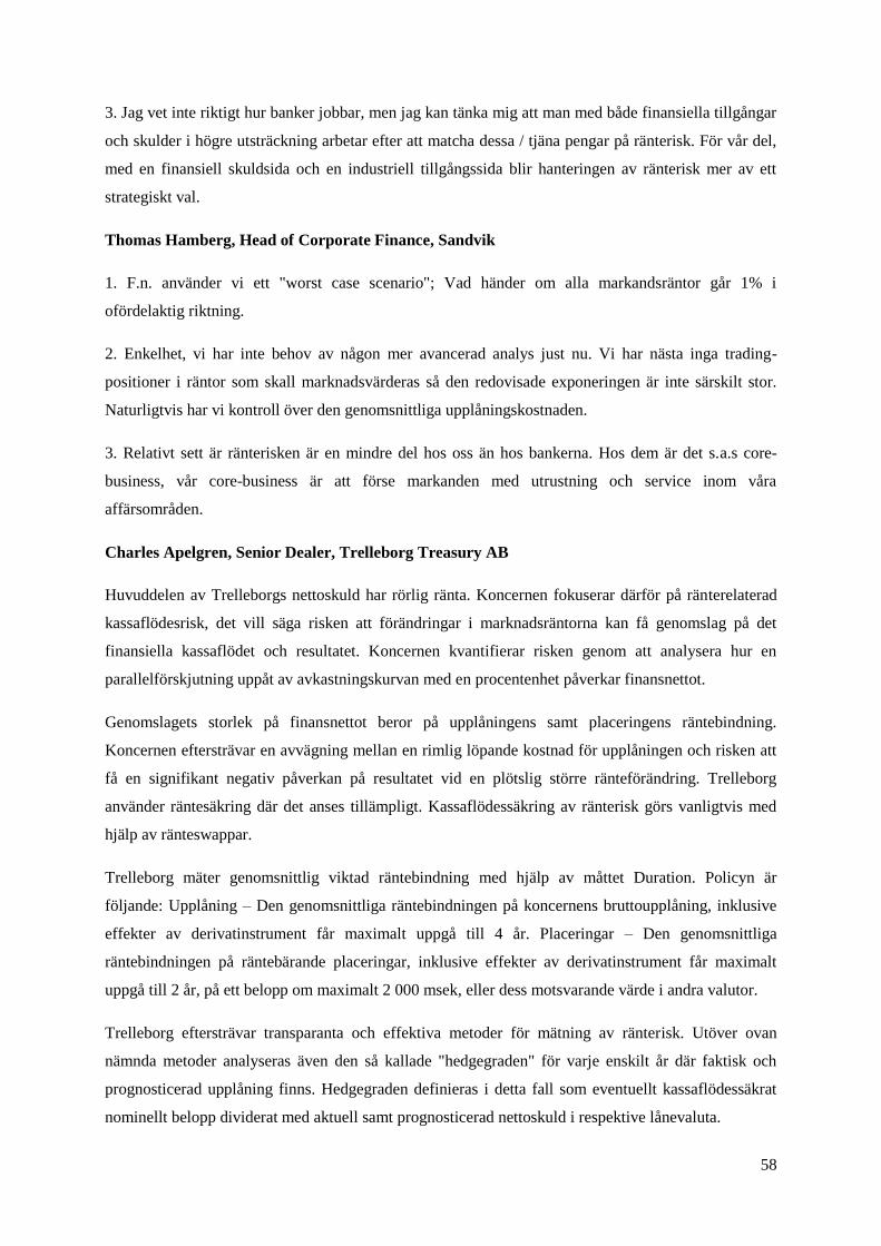
58

3. Jag vet inte riktigt hur banker jobbar, men jag kan tänka mig att man med både finansiella tillgångar

och skulder i högre utsträckning arbetar efter att matcha dessa / tjäna pengar på ränterisk. För vår del,

med en finansiell skuldsida och en industriell tillgångssida blir hanteringen av ränterisk mer av ett

strategiskt val.

Thomas Hamberg, Head of Corporate Finance, Sandvik

1. F.n. använder vi ett "worst case scenario"; Vad händer om alla markandsräntor går 1% i

ofördelaktig riktning.

2. Enkelhet, vi har inte behov av någon mer avancerad analys just nu. Vi har nästa inga trading-

positioner i räntor som skall marknadsvärderas så den redovisade exponeringen är inte särskilt stor.

Naturligtvis har vi kontroll över den genomsnittliga upplåningskostnaden.

3. Relativt sett är ränterisken är en mindre del hos oss än hos bankerna. Hos dem är det s.a.s core-

business, vår core-business är att förse markanden med utrustning och service inom våra

affärsområden.

Charles Apelgren, Senior Dealer, Trelleborg Treasury AB

Huvuddelen av Trelleborgs nettoskuld har rörlig ränta. Koncernen fokuserar därför på ränterelaterad

kassaflödesrisk, det vill säga risken att förändringar i marknadsräntorna kan få genomslag på det

finansiella kassaflödet och resultatet. Koncernen kvantifierar risken genom att analysera hur en

parallelförskjutning uppåt av avkastningskurvan med en procentenhet påverkar finansnettot.

Genomslagets storlek på finansnettot beror på upplåningens samt placeringens räntebindning.

Koncernen eftersträvar en avvägning mellan en rimlig löpande kostnad för upplåningen och risken att

få en signifikant negativ påverkan på resultatet vid en plötslig större ränteförändring. Trelleborg

använder räntesäkring där det anses tillämpligt. Kassaflödessäkring av ränterisk görs vanligtvis med

hjälp av ränteswappar.

Trelleborg mäter genomsnittlig viktad räntebindning med hjälp av måttet Duration. Policyn är

följande: Upplåning – Den genomsnittliga räntebindningen på koncernens bruttoupplåning, inklusive

effekter av derivatinstrument får maximalt uppgå till 4 år. Placeringar – Den genomsnittliga

räntebindningen på räntebärande placeringar, inklusive effekter av derivatinstrument får maximalt

uppgå till 2 år, på ett belopp om maximalt 2 000 msek, eller dess motsvarande värde i andra valutor.

Trelleborg eftersträvar transparanta och effektiva metoder för mätning av ränterisk. Utöver ovan

nämnda metoder analyseras även den så kallade "hedgegraden" för varje enskilt år där faktisk och

prognosticerad upplåning finns. Hedgegraden definieras i detta fall som eventuellt kassaflödessäkrat

nominellt belopp dividerat med aktuell samt prognosticerad nettoskuld i respektive lånevaluta.

59

Den största skillnaden mellan ett industribolags treasuryavdelning och en affärsbank skulle jag säga är

att en affärsbanks huvudsakliga uppgift är att tjäna pengar på pengar. Ett industribolags

treasuryavdelning fokuserar normalt på att minimera finansiella risker för att på så sätt stödja

kärnverksamheten vilket i Trelleborgs fall är att leverera och utveckla högpresterande lösningar som

tätar, dämpar och skyddar i krävande industriella miljöer. Trelleborg Treasury AB ger även

internbanksservice till dotterbolag till självkostnadspris.

Group Treasurer, anonymous company

1. Vi använder ett durationsmått i vår tillgångs och skuldförvaltning. Till detta har vi adderat ett

avvikelsemandat uttryckt i antal månader.

2. Durationsmått är ett ganska enkelt mått och det är även lätt att kommunicera.

3. Skillnaderna mot en affärsbank är stora. En bank har som affärsidé att låna in pengar till lägsta

möjliga kostnad och låna ut till högsta möjliga avkastning givet en rimlig risknivå. Affärsidén är att

utveckla och sälja avancerade produkter. För detta krävs kapital. Målsättningen är att så långt som

möjlighet försöka få kunderna att betala oss i den takt vi upparbetar kostnader. Därigenom utgör

ränterisken en mindre del av våra totala risker.

Dealer and Risk Manager, anonymous company

1. Vi använder oss av två metoder för att mäta ränterisk i vår management rapportering:

i VaR 95%-konfidensintervall och 3dagars tidshorizont

Anledningen till de inställningana är att vi bedömer att det skulle ta oss ca 3 dagar att komma ur

en position om marknaden "skiter sig" och 95% nivån tror jag beslutades efter en allmän

rekommendation från finansinspektionen för länge sen.

ii En stresstestning där vi stressar räntekurvan med +/-1% i samtliga valutor och löptider

Samma sak här så har FI rekommenderat detta i en bok som jag tror heter "Bank och Försäkring"

utgiven av FARs (osäker på dett amen jag vet hur boken ser ut..)

2. VaR har vi valt för att det är ett ganska vedertaget begrepp och lätt att kommunicera till

management, det är lättare att förstå sig på en siffra som man maximalt kan förlora under en viss

tidshorisont (givet vissa förutsättningar) än att sitta och prata delta mot olika valutor och swapkurvor.

Det man ska ha med sig är att VaR i princip bara är ett management rapporteringsmått, ingenting som

man direkt kan analysera var på kurvan eller hur man ska positionera sig för att minska risken.

60

Stresstestet blir en form av validerings mått till VaRen där man då faktiskt pressar kurvan åt olika håll

för att då bedöma hur mycket pengar det kostar (eller marknadsvärdesförändring om man är noggran).

Det ger en lite mer nyanserad bild av var riskerna finns.

Så valet här beror på kommunicerbarhet och komplexitet.

3. Största skillnaden mellan oss och en affärsbank, som jag ser det, är att vår råvara är

industriproduktion av lastbilar, vi har en fysisk produkt bakom allt vi gör. Medans affärsbankernas

råvara är kapital och infrastruktur för pengar och finansiella produkter. Vi finns till för att stötta

lastbilsproduktion och försäljning.

Eftersom vårt huvuduppdrag inte är att positionera oss på den finansiellamarknaden så ska vi i teorin

ligga och matcha krona för krona när det gäller faktiska flöden som uppkommer vi lastbilsförsäljning,

i detta har vi en viss frihet eftersom det i praktiken är ogörligt. En affärsbank å andra sidan har ju ett

egenintresse av att tjäna pengar på positionernig i marknaden samt att matcha olika kunders flöden och

förväntningar på tex ränteutvecklingen.

Jag tror att vi är mer riskaverta än banker generellt och matchar vår räntebindning mellan tillgånga och

skullder bättre än banker (hur skulle annars de förlora så mycket pengar vid stigande kreditspreadar???

Jag anar att de i ganska stor utsträckning ligger och rider yield-kurvan). Men jag tror å andra sidan att

de använder ungefär samma metoder som vi när det gäller mått och bedömning av ränterisken per-se.

Utöver VaR och Stresstestning så ligger vi som jobbar med ränterisk och tittar på olika typer av

rapporter hela tiden som mäter vår exponering i olika tidshinkar (gap-risker) mellan valutor (Cross-

currency risker) och fixingrisker, dvs när våra respektive tillgångar och skulder räntesätts.

Lisa Haglund, Treasury Controller, Atlas Copco

1. Atlas Copco does not use any specific methods to calculate interest rate risk on a daily basis as we

do not have any larger exposure (propriety trading). We favor a short interest rate duration, and

generally swaps fixed interest rates to floating rates. While short interest rate duration results in more

volatility of the net interest cost compared to fixed rates (long duration), high interest rates have

historically tended to reflect a strong general economic environment in which the Group enjoys strong

profits and thereby can absorb higher interest costs. Therefore the guidelines states that the average

interest rate duration should be a minimum of 6 months and a maximum of 36 months, with a

benchmark of 12 months.

2. See above. By favoring short term interest duration, we are able to follow the economic

environment.

61

3. First of all, Atlas Copco does not do any propriety trading. We are also mainly dealing with internal

counterparties, and for that we do not need to take counterparty risk into consideration. We have no

goal to make money on our loans/deposits, and can also set the rules of the lending.

measuring interest rate risk in the treasury operations of an international industrial company

Documents