measuring inequality with ordinal datadse.univr.it/it/documents/it10/canazei_2015_cowell_web.pdf ·...

Motivation Approach Inequality Measures Empirical aspects Summary References

Measuring Inequality with Ordinal data

Frank Cowellhttp://darp.lse.ac.uk/cowell.htm

Università di Verona: Alba di CanazeiWinter School

January 2015

http://darp.lse.ac.uk/cowell.htm


OutlineMotivation

Introduction and Previous workBasicsExamples

ApproachModelCharacterisation

Inequality MeasuresMain propertiesSensitivity

Empirical aspectsImplementationPerformanceApplication

Summary


Introduction

• Ordinal data issue widespread in inequality analysis• Many applications proceed just as though cardinal:

• life satisfaction / inequality of happiness: Oswald and Wu (2011),Stevenson and Wolfers (2008b), Yang (2008)

• health status: Van Doorslaer and Jones (2003)

• Small literature that takes ordinal problem seriously

• early approaches using 1st order dominance, the median• Abul Naga and Yalcin (2008,2010), Allison and Foster (2004), Zheng

(2011)• but these have limitations

• Present approach based on Cowell and Flachaire (2014)


Income Inequality

• 3 ingredients:

• “income”: family income, earnings, wealth x ∈ X ⊆ R.• “income-receiving unit”: n persons• method of aggregation: function Xn→ R

• Usually work with Xnµ ⊂R

• Xnµ : Distributions obtainable from a given total income nµ using

lump-sum transfers

• Obviously can’t do that here: µ is undefined


UtilityCardinalisation and inequality

• 3 ingredients:• “income”: u = U (x).• “income-receiving unit”: n persons (as before)• method of aggregation: function Un→ R

• Problem of cardinalisation

• But just assuming cardinal utility is no use• Already pointed out in Atkinson (1970)• Dalton (1920) suggested inequality of (cardinal) utility• But if, for all i, you multiply ui by λ ∈ (0,1) and add

δ = µ[1−λ ]...• ...this will automatically reduce measured inequality.

• Is this just a technicality?• Can we proceed just as with regular income?


Categorical variableExample: Access to Services

Case 1 Case 2nk nk

Both Gas and Electricity 25 0Electricity only 25 50Gas only 25 50Neither 25 0

• Suppose we have no information about needs / usage

• It seems clear that Case 1 is more unequal than Case 2


Example self-reported health

• World Health Survey (WHS)• a general population survey• developed by WHO

• Question: Health State Descriptions• overall health• including both physical and mental health

• In general, how would you rate your health today?• Very good• Good• Moderate• Bad• Very Bad

• Compare distributions across countries


SRH Results: four countries

Austria UK Mexico Bangladeshnumber of responses

Very good 423 318 7193 494Good 390 498 18112 1949

Moderate 200 278 11221 2132Bad 36 82 2002 741

Very bad 4 17 218 228

• For all countries: rank categories in order

• For each country: compute freq distributions across categories

• How to evaluate inequality?


SRH Inequality: Gini

At UK Mx BD(1,2,3,4,5) 0.111 0.130 0.116 0.154 (BD,UK,Mx,At)

(1,2,3,4,1000) 0.593 0.725 0.800 0.884 (BD,Mx,UK,At)

(-1000,2,3,4,5) 0.608 0.821 0.856 2.377 (BD,Mx,UK,At)


SRH Inequality: Coeff of Variation

At UK Mx BD(1,2,3,4,5) 0.209 0.244 0.219 0.287 (BD,UK,Mx,At)

(1,2,3,4,1000) 1.210 1.638 2.056 3.088 (BD,Mx,UK,At)

(-1000,2,3,4,5) 187.5 11.43 40.45 5.264 (At,Mx,UK,BD)


Status and Information

• Step 1 is to define status• depends on the purpose of inequality analysis• depends on structure of information• conventional inequality approach only works in narrowly defined

information structure

• In some cases a person’s status is self-defining• income• wealth

• In some cases defined given additional distribution-freeinformation

• example: if it is known that utility is log(x)

• In some cases requires information on distribution• GRE, TOEFL• “opportunity” (de Barros et al. 2008)


Status and Distribution (1)

• i’s status uniquely defined for a given distribution of u

u = U(x)

u2

1

v = V(x)v2u1 v1

s1

s2

u = U(x)

u2

1

v = V(x)v2u1 v1

s1

s2

• disposes of the problem of cardinalisation• U and V = ϕ (U) two cardinalisations of the utility of x• for each i:ui and vi map into si


Status and distribution (2)

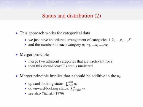
• This approach works for categorical data

• we just have an ordered arrangement of categories 1,2, ...,k, ...,K• and the numbers in each category n1,n2,...,nk,...,nK

• Merger principle

• merge two adjacent categories that are irrelevant for i• then this should leave i’s status unaltered

• Merger principle implies that s should be additive in the nk

• upward-looking status: ∑k(i)`=1 n`

• downward-looking status: ∑K`=k(i) n`

• see also Yitzhaki (1979)


Elements of the Model

• Individual’s status is given by s ∈ S⊆ R• status determined from utility?

• Vector of status in a population of size n : s ∈ Sn

• e ∈ S : an equality-reference point

• could be specified exogenously• could also depend on status vector e = η (s)• η need not be increasing in each component of s

• Inequality: aggregate distance from e

• don’t need an explicit distance function

• implicitly define through inequality ordering �


Basic Axioms

• [Continuity] � is continuous on Sn

• [Monotonicity] If s,s′ ∈ Sne differ only in their ith component

then (a) if s′i ≥ e :si > s′i⇐⇒ s� s′; (b) if s′i ≤ e:s′i > si⇐⇒ s� s′

• [Independence] For s,s′ ∈ Sne , if s ∼ s′ and si = s′i for some i

then s(ς , i)∼ s′ (ς , i) for all ς ∈ [si−1,si+1]∩[s′i−1,s

′i+1

]• [Anonymity] For all s ∈ Sn and permutation matrix P, Ps ∼s .


Standard result

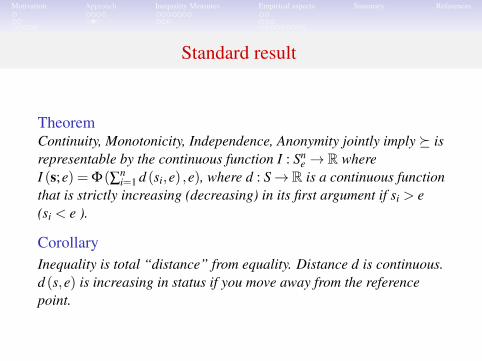
TheoremContinuity, Monotonicity, Independence, Anonymity jointly imply � isrepresentable by the continuous function I : Sn

e → R whereI (s;e) = Φ(∑n

i=1 d (si,e) ,e), where d : S→ R is a continuous functionthat is strictly increasing (decreasing) in its first argument if si > e(si < e ).

CorollaryInequality is total “distance” from equality. Distance d is continuous.d (s,e) is increasing in status if you move away from the referencepoint.


Structure Theorem

• We need more structure on the problem

• [Scale invariance 1] For all λ ∈ R+: if s,s′,λ s,λ s′ ∈ Sn ande,e′ ∈ S then (s,e)∼ (s′,e′)⇒(λ s,e)∼ (λ s′,e′) .

• [Scale invariance 2] For all λ ∈ R+: if s,s′,λ s,λ s′ ∈ Sn ande,e′,λe,λe′ ∈ S then (s,e)∼ (s′,e′)⇒(λ s,λe)∼ (λ s′,λe′)

TheoremImpose also Scale irrelevance 1. Then d (s,e) = A(e)sα(e)

TheoremImpose instead Scale Invariance 2. Then d (s,e) = eβ φ

( se

).where β

is a constant and φ is arbitrary

CorollaryInequality represented as Iα (s;e) := 1

α[α−1]

[1n ∑

ni=1 sα

i − eα]


A usable inequality index?

• A class of functions available as inequality measures:

• Φ(Iα (s;e) ,e)• e = η (s) , the reference point• Iα (s;e) := 1

α[α−1]

[ 1n ∑

ni=1 sα

i − eα]

• Do functions Φ(Iα (s;e) ,e) “look like” inequality measures?

• transfer principle?• reference point?• sensitivity to parameters

• What is the appropriate form for Φ?

• may depend on the reference status e• may depend on interpretation


Four distributional scenarios (1)

Case 0 Case 1 Case 2 Case 3nk si nk si nk si nk si

B 0 25 1 0 25 1E 50 1 25 3/4 50 1 25 3/4

G 25 1/2 25 1/2 50 1/2 50 1/2

N 25 1/4 25 1/4 0 0

µ(s) 11/16 5/8 3/4 11/16

• nk is # persons in category k ∈ {B,E,G,N}

• si =1n ∑

k(i)`=1 n` – downward-looking status


Four distributional scenarios

Case 0 Case 1 Case 2 Case 3nk s′i nk s′i nk s′i nk s′i

B 0 25 1/4 0 25 1/4

E 50 1/2 25 1/2 50 1/2 25 1/2

G 25 3/4 25 3/4 50 1 50 1N 25 1 25 1 0 0

µ(s) 11/16 5/8 3/4 11/16

• nk is # persons in category k ∈ {B,E,G,N}

• s′i =1n ∑

K`=k(i) n` – upward-looking status




B 0 25 1 0 25 1E 50 1 25 3/4 50 1 25 3/4

G 25 1/2 25 1/2 50 1/2 50 1/2

N 25 1/4 25 1/4 0 0

µ(s) 11/16 5/8 3/4 11/16

• Case 0 to Case 1:

• 25 people promoted from E to B• if e equals to any of values taken by µ(s)• then inequality increases




B 0 25 1 0 25 1E 50 1 25 3/4 50 1 25 3/4

G 25 1/2 25 1/2 50 1/2 50 1/2

N 25 1/4 25 1/4 0 0

µ(s) 11/16 5/8 3/4 11/16

• Case 0 to Case 2:

• 25 people promoted from N to G• if e equals to any of values taken by µ(s)• then inequality decreases


Transfer Principle again


B 0 25 1 0 25 1E 50 1 25 3/4 50 1 25 3/4

G 25 1/2 25 1/2 50 1/2 50 1/2

N 25 1/4 25 1/4 0 0

µ(s) 11/16 5/8 3/4 11/16

• Case 0 to Case 1: inequality increases• Case 0 to Case 2: inequality decreases• Case 0 to Case 3: combination results in ambiguous change


Reference point

• Mean status: e = η (s) = µ(s)• for continuous distributions will equal 0.5• for categorical data, there is no counterpart to fixed-mean

assumption in income-inequality analysis

• Median status: e = η (s) = med(s)• not well-defined: any value in interval M (s)• M (s) = [1/2,1) in cases 0 and 2• M (s) = [1/2,3/4) in cases 1 and 3

• Max status: e = 1• for constant e this is only value that makes sense

• Min status: e = 0• counterpart for peer-exclusive case


Sensitivity

• α captures the sensitivity of measured inequality

• If α is high Iα (s;e) = 1α[α−1]

[1n ∑

ni=1 sα

i − eα], sensitive to high

status-inequality

• If α = 0 then I0 (s;e) =−1n ∑

ni=1 logsi + loge,

• If e = µ(s) and α = 1 then 1n ∑

ni=1 si logsi− e loge


Behaviour of I0 (s;e)

Case 0 Case 1 Case 2 Case 3µ(s) 11/16 5/8 3/4 11/16

med1(s) 3/4 5/8 3/4 5/8

med2(s) 1/2 1/2 1/2 1/2

I0(s; µ (s)) 0.1451 0.1217 0.0588 0.0438I0(s; med1(s)) 0.2321 0.1217 0.0588 -0.0515I0(s; med2(s)) -0.1732 -0.1013 -0.3465 -0.2746

I0(s; 1) 0.5198 0.5917 0.3465 0.4184

• I0(s; µ (s)), I0(s; med1(s)): inequality decreases for• Case 0 to 1, or Case 2 to 3• movement changes both the µ (s) and med1 (s) ref points

• I0(s; med2(s))< 0 for all cases in example!

• But I0 (s;1) seems sensible


Inequality measure

• For ordinal data, peer-inclusive status

• Iα(s,1) =

1

α(α−1)

[1n ∑

ni=1 sα

i −1], if α 6=0, α<1

−1n ∑

ni=1 logsi. if α=0

●●●●●●●●●●●●●●●●●●●●●●●●●●●●●●●●●●●●●●●●●●●●●●●●●●●●●●●●●●●●●●●●●●●●●●●●●●●●●●●●●●●●●●●●●●●●●●●●●●●●●●●●●●●●●●●●●●●●●●●●●●●●●●●●●●●●●●●●●●●●●●●●●●●●●●●●●●●●●●●●●●●●●●●●●●●●●●●●●●●●●●●●●●●●●●●●●●●●●●●●●●●●●●●●●●●●●●●●●●●●●●●●●●●●●●●●●●●●●●●●●●●●●●●●●●●●●●●●●●●●●●●●●●●●●●●●●●●●●●●●●●●●●●●●●●●●●●●●●●●●●●●●●●●●●●●●●●●●●●●●●●●●●●●●●●●●●●●●●●●●●●●●●●●●●●●●●●●●●●●●●●●●●●●●●●●●●●●●●●●●●●●●●●●●●●●●●●●●●●●●●●●●●●●●●●●●●●●●●●●●●●●●●●●●●●●●●●●●●●●●●●●●●●●●●●●●●●●●●●●●●●●●●●●●●●●●

●●●●●●●●●●●●●●●●●●●●●●●●●●●●●●●●●●●●●●●●●●●●●●●●●●●●●●●●●●●●●●●

●

●

●

●

●

●

●

●

●

●

●

●

●●●●●●●●●●●●●●●●●●●●●●●●●●●●●●●●●●●●●●●●●●●●●●●●●●●●●●●●●●●●●●●●●

●●●●●●●●●●●●●●●●●●●●●●●●●●●●●●●●●●●●●●●●●●●●

●●●●●●●●●●●●●●●●●●●●●●●●●●●●●●●●●●●●●●●●●●●●●●●●●●●●●●●●●●●●●●●●●●●●●●●●●●●●●●●●●●●●●●●●●●●●●●●●●●●●●●●●●●●●●●●●●●●●●●●●●●●●●●●●●●●●●●●●●●●●●●●●●●●●●●●●●●●●●●●●●●●●●●●●●●●●●●●●●●●●●●●●●●●●●●●●●●●●●●●●●●●●●●●●●●●●●●●●

●●●●●●●●●●●●●●●●●●●●●●●●●●●●●●●●●●●●●●●●●●●●●●●●●●●●●●●●●●●●●●

−4 −2 0 2 4

−2

−1

01

23

4

alpha

I


Implementation

• Description of sample

xi =

1 with sample proportion p1

2 with sample proportion p2

. . .

K with sample proportion pK

,

• Point estimate of the index:

• Iα =

1

α(α−1)

[∑

Ki=1 pi

[∑

ij=1 pj

]α

−1]

if α 6=0,1

−∑Ki=1 pi log

[∑

ij=1 pj

]if α=0

• function of K parameter estimates (p1,p2, . . . ,pK) following amultinomial


Asymptotics

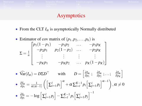
• From the CLT Iα is asymptotically Normally distributed

• Estimator of cov matrix of (p1,p2, . . . ,pk) is

Σ = 1n

p1(1−p1) −p1p2 . . . −p1pK

−p2p1 p2(1−p2) . . . −p2pK...

......

...−pKp1 −pKp2 . . . pK(1−pK)

• V̂ar(Iα) = DΣD> with D =

[∂ Iα

∂p1; ∂ Iα

∂p2; . . . ; ∂ Iα

∂pK

]• ∂ Iα

∂pl= 1

α(α−1)

([∑

li=1 pi

]α

+α ∑K−1i=l pi

[∑

ij=1 pj

]α−1),α 6= 0

• ∂ I0∂pl

=− log[

∑lj=1 pj

]−∑

K−1i=l pi

[∑

ij=1 pj

]−1


Confidence Intervals

• 3 variants of CIs: Asymptotic, Percentile Bootstrap, StudentizedBootstrap

• CIasym = [Iα − c0.975V̂ar(Iα)1/2 ; Iα + c0.975V̂ar(Iα)

1/2]

• c0.975 from the Student distribution T(n−1)• do not always perform well in finite samples

• Bootstraps: generate resamples, b = 1, . . . ,B• for each resample b compute the inequality index• obtain B bootstrap statistics, Ib

α

• also B bootstrap t-statistics tbα = (Ib

α − Iα)/V̂ar(Ibα)

1/2

• CIperc = [cb0.025 ; cb

0.975]

• cb0.025 and cb

0.975 are from EDF of bootstrap statistics

• CIstud = [Iα − c∗0.975V̂ar(Iα)1/2 ; Iα − c∗0.025V̂ar(Iα)

1/2]

• c∗0.025 and c∗0.975 are from EDF of the bootstrap t-statistics


Performance Test

• Take an example with 3 ordered categories (K = 3 )

• Samples are drawn from a multinomial distribution withprobabilities π = (0.3,0.5,0.2)

• Is asymptotic or bootstrap distribution a good approximation ofthe exact distribution of the statistic?

• if we are using 95% CIs of Iα

• coverage error rate should be close to nominal rate, 0.05

• Check coverage error rate of CIs as sample size increases

• α =−1,0,0.5,0.99• 199 bootstraps• 10 000 replications to compute error rates• n = 20,50,100,200,500,1000


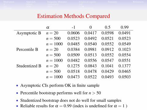
Estimation Methods Compared

α -1 0 0.5 0.99Asymptotic B n = 20 0.0606 0.0417 0.0598 0.0491

n = 500 0.0523 0.0492 0.0521 0.0523n = 1000 0.0485 0.0540 0.0552 0.0549

Percentile B n = 20 0.0384 0.0981 0.0912 0.1023n = 500 0.0509 0.0513 0.0552 0.0554n = 1000 0.0482 0.0556 0.0547 0.0551

Studentized B n = 20 0.1275 0.0843 0.1041 0.1377n = 500 0.0518 0.0478 0.0429 0.0465n = 1000 0.0473 0.0522 0.0493 0.0503

• Asymptotic CIs perform OK in finite sample

• Percentile bootstrap performs well for n > 50

• Studentized bootstrap does not do well for small samples• Reliable results for α = 0.99 (index is undefined for α = 1 )


World values survey

• Life satisfaction question:

All things considered, how satisfied are you with your life as awhole these days? Using this card on which 1 means you are“completely dissatisfied” and 10 means you are “completelysatisfied” where would you put your satisfaction with your life asa whole? (code one number):

Completely dissatisfied – 1 2 3 4 5 6 7 8 9 10 – Completely satis-

fied

• Health question:

All in all, how would you describe your state of health these days?Would you say it is (read out):

1 Very good, 2 Good, 3 Fair, 4 Poor.


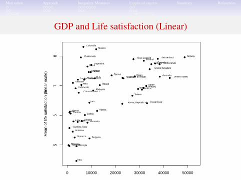
GDP and Life satisfaction

• Cross-country comparison of life satisfaction and GDP/head• happiness-income paradox (Easterlin 1974, Clark and Senik 2011)• weak relation happiness-income internationally? (Easterlin 1995,

Easterlin et al. 2010)• or a strong relationship? (Hagerty and Veenhoven 2003, Deaton 2008,

Stevenson and Wolfers 2008a, Inglehart et al. 2008)

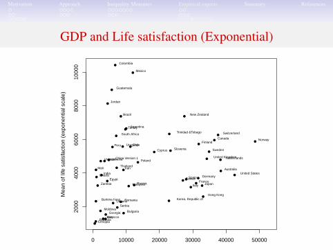
• How should we quantify life satisfaction?

• simple linearity of Likert scale? or exponential scale?• Ng (1997), Ferrer-i-Carbonell and Frijters (2004), Kristoffersen (2011)

• Is inequality of life satisfaction related to GDP/head?

• Use I0 and other members of the same family


GDP and Life satisfaction (Linear)

●

●

●

●

●

●

●

●

●

●

●

●

●

●

●

●

●

●

●

●

●

●

●

●

●

●

●

●

●

●

●

●

●

●

●

●

●●

● ●

●

●

●

●

●

●

●●

●

●

●

●

●

●

●

●

0 10000 20000 30000 40000 50000

56

78

Per capita GDP in 2005

Mea

n of

life

sat

isfa

ctio

n (li

near

sca

le)

Argentina

Australia

Burkina Faso

Bulgaria

BrazilCanada

Switzerland

Chile

China Version 1

Colombia

Cyprus

Egypt

Spain

Ethiopia

Finland

France

United Kingdom

Georgia

Germany

Ghana

Guatemala

Hong Kong

Indonesia

India

Iran

Iraq

Italy

Jordan

Japan

Korea, Republic of

Morocco

Moldova

Mexico

Mali

Malaysia

Netherlands

NorwayNew Zealand

Peru Poland

Romania

Russia

Rwanda

Serbia

Slovenia

Sweden

ThailandTrinidad &Tobago

Turkey

Taiwan

Ukraine

Uruguay

United States

VietnamSouth Africa

Zambia


GDP and Life satisfaction (Exponential)

●

●

●

●

●

●

●

●

●

●

●

●●

●

●

●

●

●

●●

●

●

●

●

●

●

●

●

●

●

●

●

●

●

●

●

●

●

●

●

●

●

●

●

● ●

●

●

●

●

●

●

●

●

●

●

0 10000 20000 30000 40000 50000

2000

4000

6000

8000

1000

0


Mea

n of

life

sat

isfa

ctio

n (e

xpon

entia

l sca

le)

Argentina

Australia

Burkina Faso

Bulgaria

Brazil

Canada

Switzerland

Chile

China Version 1

Colombia

Cyprus

Egypt Spain

Ethiopia

Finland

France

United Kingdom

Georgia

GermanyGhana

Guatemala

Hong Kong

Indonesia

India

Iran

Iraq

Italy

Jordan

Japan

Korea, Republic of

Morocco

Moldova

Mexico

Mali

Malaysia

Netherlands

Norway

New Zealand

Peru

Poland

Romania

Russia

Rwanda

Serbia

Slovenia Sweden

Thailand

Trinidad &TobagoTurkey

Taiwan

Ukraine

Uruguay

United States

Vietnam

South Africa

Zambia


GDP and Inequality of Life satisfaction

●

●

●

●

●

●

●

●

●

●

●

●

●

●

●

●

●

●

●

●

●

●

●

●

●

●

●

●

●

●

●

●

●

●

●

●

●

●

●

●

●

●

●

●

●

●

●

●●

●

●

●

●

●

●

●

0 10000 20000 30000 40000 50000

0.55

0.60

0.65

0.70

0.75

0.80


Ineq

ualit

y of

life

sat

isfa

ctio

n

Argentina

Australia

Burkina Faso

Bulgaria

Brazil

Canada

Switzerland

Chile

China Version 1

Colombia

Cyprus

Egypt

Spain

Ethiopia

Finland

France

United Kingdom

Georgia

Germany

Ghana

Guatemala

Hong Kong

Indonesia

India

Iran

Iraq

Italy

Jordan

Japan

Korea, Republic of

Morocco

Moldova

Mexico

Mali

Malaysia

Netherlands

Norway

New Zealand

Peru

Poland

Romania

Russia

Rwanda

Serbia

Slovenia

Sweden

Thailand

Trinidad &TobagoTurkey

Taiwan

Ukraine

Uruguay

United States

Vietnam

South Africa

Zambia


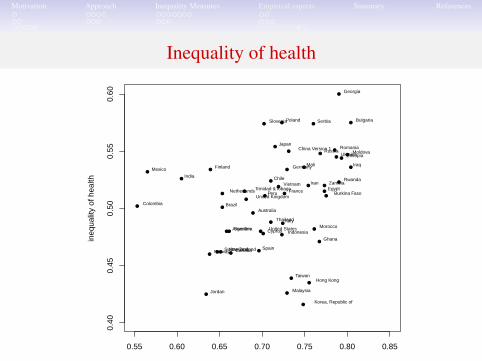
Health status

• Health is HRS

• Cross-country comparison of health and GDP• a significant positive relationship? (Deaton 2008)

• Cross-country comparison of inequality of health and Inequalityof life satisfaction

• use same inequality index as for life satisfaction


Inequality of health and GDP

●

●

●

●

●

● ●

●

●

●

●

●

●

●

●

●

●

●

●

●

●

●

●

●

●

●

●

●

●

●

●

●

●

●

●

●●

●

●

●●

●

● ●

●

●

●

●

●

●

●●

0 10000 20000 30000 40000 50000

0.40

0.45

0.50

0.55

0.60


Ineq

ualit

y of

hea

lth

Argentina

Australia

Burkina Faso

Bulgaria

Brazil

CanadaSwitzerland

Chile

China Version 1

Colombia

Cyprus

Egypt

Spain

Ethiopia

Finland

FranceUnited Kingdom

Georgia

Germany

Ghana

Hong Kong

Indonesia

India

Iran

Iraq

Italy

Jordan

Japan

Korea, Republic of

Morocco

Moldova

MexicoMali

Malaysia

Netherlands

NorwayNew Zealand

Peru

Poland

RomaniaRussia

Rwanda

Serbia Slovenia

Sweden

Thailand

Trinidad &Tobago

Taiwan

Ukraine

United States

VietnamZambia


Inequality of health

●

●

●

●

●

●●

●

●

●

●

●

●

●

●

●

●

●

●

●

●

●

●

●

●

●

●

●

●

●

●

●

●

●

●

●●

●

●

●●

●

●●

●

●

●

●

●

●

● ●

0.55 0.60 0.65 0.70 0.75 0.80 0.85

0.40

0.45

0.50

0.55

0.60

Inequality of life satisfaction

ineq

ualit

y of

hea

lth

Argentina

Australia

Burkina Faso

Bulgaria

Brazil

CanadaSwitzerland

Chile

China Version 1

Colombia

Cyprus

Egypt

Spain

Ethiopia

Finland

FranceUnited Kingdom

Georgia

Germany

Ghana

Hong Kong

Indonesia

India

Iran

Iraq

Italy

Jordan

Japan

Korea, Republic of

Morocco

Moldova

MexicoMali

Malaysia

Netherlands

NorwayNew Zealand

Peru

Poland

RomaniaRussia

Rwanda

SerbiaSlovenia

Sweden

Thailand

Trinidad &Tobago

Taiwan

Ukraine

United States

Vietnam Zambia


Application: overview

• Satisfaction / GDP results sensitive to the cardinal interpretationof the answers

• linear: positive relation below $15 000, flat after that (Layard 2003)• exponential: no relation

• OLS estimate of I0(life satisfaction) on the GDP per capita smalland negative

• happiness-income relationship is weak in cross-countrycomparisons

• No clear relationship between I0(health) on GDP per capita

• OLS estimate of I0(health) on I0(life satisfaction) produces aslope coefficient not significantly different from zero

• health-life satisfaction relationship is not significant


Summary

• Inequality with ordinal data is a widespread phenomenon

• Conventional I-measures may make no sense

• Cowell and Flachaire (2014) approach:

• separates out the issue of status from that ofinequality-aggregation

• allows you to choose “reference status”• gives a family of measures

• Nice properties empirically


Bibliography I

Abul Naga, R. H. and T. Yalcin (2008). Inequality measurement for ordered response health data. Journal of HealthEconomics 27, 1614–1625.

Abul Naga, R. H. and T. Yalcin (2010). Median independent inequality orderings. Technical report, University of AberdeenBusiness School.

Allison, R. A. and J. E. Foster (2004). Measuring health inequality using qualitative data. Journal of Health Economics 23,505–552.

Atkinson, A. B. (1970). On the measurement of inequality. Journal of Economic Theory 2, 244–263.

Clark, A. E. and C. Senik (2011). Will GDP growth increase happiness in developing countries? In J. Slemrod (Ed.),Measure For Measure: How well do we Measure Development? AFD Publications.

Cowell, F. A. and E. Flachaire (2014). Inequality with ordinal data. Public Economics Programme Discussion Paper 16,London School of Economics, http://darp.lse.ac.uk/pdf/IneqOrdinal.pdf.

Dalton, H. (1920). Measurement of the inequality of incomes. The Economic Journal 30, 348–361.

de Barros, R. P., F. Ferreira, J. Chanduvi, and J. Vega (2008). Measuring Inequality of Opportunities in Latin America andthe Caribbean. Palgrave Macmillan.

Deaton, A. (2008). Income, health and well-being around the world: Evidence from the Gallup World Poll. Journal ofEconomic Perspectives 22, 53–72.

Easterlin, R. A. (1974). Does economic growth improve the human lot? Some empirical evidence. In P. A. David and M. W.Reder (Eds.), Nations and Households in Economic Growth: Essays in Honor of Moses Abramovitz. New York:Academic Press.


Bibliography II

Easterlin, R. A. (1995). Will raising the incomes of all increase the happiness of all? Journal of Economic Behavior &Organization 27, 35–47.

Easterlin, R. A., L. Angelescu McVey, M. Switek, O. Sawangfa, and J. Smith Zweig (2010). The happiness-income paradoxrevisited. Proceedings of the National Academy of Sciences of the United States of America 107, 22463–22468.

Ferrer-i-Carbonell, A. and P. Frijters (2004). How important is methodology for the estimates of the determinants ofhappiness? The Economic Journal 114, 641–659.

Hagerty, M. R. and R. Veenhoven (2003). Wealth and happiness revisited: Growing wealth of nations does go with greaterhappiness. Social Indicators Research 64, 1–27.

Inglehart, R., R. Foa, C. Peterson, and C. Welzel (2008). Development, freedom, and rising happiness: A global perspective(1981-2007). Perspectives on Psychological Science 3, 264–285.

Kristoffersen, I. (2011). The subjective wellbeing scale: How reasonable is the cardinality assumption? DiscussionPaper 15, University of Western Australia Department of Economics.

Layard, R. (2003). Happiness: Has social science a clue. Lionel Robbins Memorial Lectures 2002/3, London School ofEconomics, march 3-5. http://cep.lse.ac.uk/events/lectures/layard/RL030303.pdf.

Ng, Y. K. (1997). A case for happiness, cardinalism, and interpersonal comparability. The Economic Journal 107, 1848–58.

Oswald, A. J. and S. Wu (2011, November). Well-being across America. The Review of Economics and Statistics 93(4),1118–1134.

Stevenson, B. and J. Wolfers (2008a). Economic growth and subjective well-being: Reassessing the Easterlin paradox.NBER working paper no. 14282.


Bibliography IIIStevenson, B. and J. Wolfers (2008b). Happiness inequality in the United States. The Journal of Legal Studies 37, S33–S79.

Van Doorslaer, E. and A. M. Jones (2003). Inequalities in self-reported health: Validation of a new approach tomeasurement. Journal of Health Economics 22, 61–87.

Yang, Y. (2008). Social inequalities in happiness in the United States, 1972 to 2004: An age-period-cohort analysis.American Sociological Review 73, 204–226.

Yitzhaki, S. (1979). Relative deprivation and the Gini coefficient. Quarterly Journal of Economics 93, 321–324.

Zheng, B. (2011). A new approach to measure socioeconomic inequality in health. Journal Of Economic Inequality 9,555–577.

measuring inequality with ordinal datadse.univr.it/it/documents/it10/canazei_2015_cowell_web.pdf ·...

Documents