measuring district level partisanship with implications ... · measuring district level...
TRANSCRIPT

Measuring District Level Partisanship
with Implications for the Analysis of U.S. Elections∗
Matthew S. Levendusky†, Jeremy C. Pope‡, and Simon D. Jackman§
March 2, 2008
∗We thank Chris Achen, Daniel Bergan, David Brady, Jay Goodliffe, John Jackson, Gary King, Keith Poole, Doug
Rivers, Howard Rosenthal, participants at the 2003 and 2005 Political Methodology Society Meetings and the Stanford
Measurement Conference (August 2003) for useful comments. We also thank E. Scott Adler, Brandice Canes-Wrone,
Joshua Clinton, John Cogan, Gary Jacobson, Stephen Ansolabehere and Jim Snyder, and most of all, David Brady for
generously providing us with access to their data.†Assistant Professor, Department of Political Science, University of Pennsylvania.‡Assistant Professor, Department of Political Science, and Research Fellow, Center for the Study of Elections and
Democracy, Brigham Young University.§Professor and Director, Political Science Computational Laboratory, Department of Political Science, Stanford
University.

Abstract
Studies of American politics, particularly legislative politics, rely heavily on measures of the
partisanship of a district. We develop a measurement model for this concept, estimating parti-
sanship in the absence of a election-specific, short-term factors, such as national-level swings
specific to particular elections, incumbency advantage, and home-state effects in presidential
elections. We estimate the measurement model using electoral returns and district-level demo-
graphic characteristics spanning five decades (1952-2000), letting us assess how the distribution
of district partisanship has changed over time, in response to population movements and redis-
tricting, particularly via the creation of majority-minority districts. We validate the partisanship
measure with an analysis of Congressional roll call data. The model is easily extended to incor-
porate other indicators of district partisanship, such as survey data.
2
Almost all empirical studies of Congressional elections rely on a measure of district partisanship,
be they studies of incumbency advantage (e.g., Gelman and King 1990), challenger effects (e.g.,
Jacobson and Kernell 1983), redistricting (e.g., Cox and Katz 1999), regional differences in the
electorate, or national forces in elections (e.g., Kawato 1987). These analyses share a common
methodological strategy: estimating the effects of more or less transient factors (e.g., candidates and
issues) on the vote by statistically controlling for the partisan or ideological disposition of a district.
These studies stand or fall on the quality of the measure of district partisanship. Consider a regression
of district level vote shares on variables of substantive interest and a control for district partisanship.
If the district partisanship measure is measured with error, then not only is the coefficient on district
partisanship biased, but so too is the coefficient on any variable correlated with district partisanship,
either directly or indirectly. Thus, an approach that better measures the underlying concept —
district partisanship — can improve estimation of all of those quantities, and enhance the validity of
substantive conclusions. In this paper we provide such a measure.
District Partisanship: Theory and Measurement
Our approach rests upon decomposing voting behavior into long-term and short-term compo-
nents, an approach with a long and distinguished lineage in political science, dating at least to Con-
verse’s (1966) concept of the “normal vote.” The normal vote grows directly out of the Michigan
team’s micro-model of voting behavior, in which party identification generates stability in voting
behavior, subject to election-specific responses to candidates and issues. The normal vote is the
aggregate-level analog of enduring micro-level political loyalties, and rests on decomposing vote
shares into two components: a long-term, stable component driven by party identification (the nor-
mal vote), and a short-term rate of defection generated by the specifics of the campaign and the
candidates (Converse 1966, 14).1 Our measure of district partisanship is analogous to Converse’s
1The majority of work using the concept of a normal vote has followed Converse’s initial ap-
proach and used survey data, examining rates of party voting within and across categories of parti-
san identifiers (e.g., Goldenberg and Traugott 1981; Petrocik 1989). This approach has been rightly
3

normal vote, except that Converse operationalized the concept with survey data on voting and party
identification, whereas our measure relies on a mix of aggregate indicators (and in the extensions
discussed in the on-line Appendix, survey data). Like Converse, we seek to identify the more-or-
less stable partisan force driving election outcomes. As such, our measure of district partisanship
provides an estimate of how Democratic a given district would be absent the impact of a given cam-
paign (election-specific partisan swings, incumbency, etc.). That is, without any short-term forces,
how Democratic or Republican would a given district be?
We also want to be clear about what it is we are not measuring. Measurement models use ob-
served variables to make inferences about latent variables. Consequently, the latent variable inherits
its substantive content from the indicators available for analysis and our modeling assumptions. In
our case, since we rely heavily on district level vote shares as indicators, the substantive content of
our recovered latent trait can not stray far from whatever substantive content resides in vote shares
(or the determinants of vote shares). Given that we have data on vote shares, but not, say, survey
data, we will resist claiming that we validly measure “district ideology”. Of course, to the extent that
presidential and congressional voting is driven by ideology, then our measure will have ideological
content. For now, using only vote shares (as opposed to, say, survey data on individual preferences),
we take a conservative approach and interpret our measure as district partisanship rather than district
ideology. However, in the on-line appendix, we augment our model with survey measures of ide-
ology to demonstrate one approach to validly estimating district ideology. Likewise, we will resist
stating that our model provides valid estimates of district preferences, such as the relative locations
of each district’s median/mean voter. Our measurement model does not operationalize a structural
voting model that maps from voter ideal points on a policy continuum to district level vote shares.
subject to criticism, on the grounds that party identification is not exogenous, but responds to the
same short term forces that shape vote decisions in any given election (e.g., Achen 1979). We stress
that although Converse’s concept of a normal vote underlies our approach, our goal is to measure
district partisanship (or the normal vote) at the level of congressional districts, and we do so with
aggregate data, with a set of controls that let us decompose vote shares into short-term and long-term
components.
4

While it would no doubt be worthwhile to investigate such a model (e.g., Snyder 2005), that endeav-
our is beyond our current scope.
Previous work has employed roughly three types of measures for district partisanship: surveys,
election returns, and demographic data. Each method has significant limitations.
(1) Survey-based methods. Almost all survey based methods suffer from a profound design
challenge, sometimes referred to as the “Miller-Stokes problem”. Miller and Stokes (1963) were
interested in the extent to which members of Congress responded to district opinion. But the data
they had for any individual congressional district was extremely sparse; their study used a national
probability sample that had an average of only 13 respondents per congressional district (see Achen
1978; Erikson 1978). And in general, generating representative samples of useful sizes from a useful
number of congressional districts is very difficult, given the data gathering technologies and research
budgets typically available to political scientists.2 With a given budget constraint, researchers face an
obvious tradeoff between surveying fewer respondents in more districts (sacrificing within-district
precision for cross-district coverage) or surveying more respondents in fewer districts (buying pre-
cision at the cost of coverage); see Stoker and Bowers (2002) for an elaboration. In the face of
limited research budgets either coverage or precision must suffer, and hence most attempts to gen-
erate measures of partisanship (or preferences) specific to congressional districts rely on aggregate
data.3
2Clinton (2006) is a rare exception, exploiting the unusual confluence of two large studies of
the American electorate in 2000 (the Annenberg National Election Survey and a large panel of on-
line respondents from Knowledge Networks) to yield estimates of district with an average of 232
respondents per district.3Ardoin and Garand (2003) propose a novel application of survey data to this problem: using the
Wright, Erickson, and McIver (1985) state-level measures, they use the connection between demo-
graphic variables and this ideology measure to form district level estimates of constituent ideology
for the 1980s and 1990s. While the method is an excellent application of survey data, it is lim-
ited in that it can only generate results for the 1980s and 1990s due to question wording changes.
The method we present below, on the other hand, covers the entire post-war period and uses easily
5

(2) Demographic Aggregates. Examples of this measurement strategy include Kalt and Zu-
pan’s (1984) analysis of specific industries capturing members of Congress: in their analysis of
Senate voting on strip mining regulation, Kalt and Zupan took state-level data on membership in
pro-environmental interest groups and the size of various coal producer and consumer groups as
indicative of economic interests and preferences over regulation, inter alia. In a more general anal-
ysis, Peltzman (1984) used six demographic variables measured at the county level to tap politically
relevant, economic characteristics of senators’ constituencies.
A measure of district partisanship that relied solely on demographic characteristics of the dis-
trict suffers from an obvious threat to validity. Demographic attributes are generally considered
antecedents of partisanship, rather than indicators of it. So, while demographic characteristics may
correlate highly with one another and would appear to measure something about districts, there is no
guarantee that demographic characteristics alone would permit us to locate congressional districts
on a partisan continuum. That is, the use of demographics alone may generate a measure of district
partisanship with high reliability, but dubious concept validity.
(3) Electoral Returns. Election returns are popular and easily accessed proxies for district par-
tisanship. For instance, Canes-Wrone, Cogan, and Brady (2002), Ansolabehere, Snyder and Stewart
(2001), and Erickson and Wright (1980) all use district level presidential election returns as a proxy
for district partisanship in models of legislative politics. The virtue of this proxy is that it is based
on constituent behavior (vote choices) and is thus linked to the partisan or ideological continuum
that generally underlies electoral competition. Thus, a measure of district partisanship utilizing vote
shares can be assumed to have high validity. But there are shortcomings and trade-offs here as well.
Presidential vote shares in any given election may be products of short-term forces; for instance,
different issues are more or less salient in any given election, and particular candidates are more
or less popular. And over the long-run, averaging a district’s presidential vote shares may well be
a valid (i.e., unbiased) indicator of district partisanship over the same period (e.g., Ansolabehere,
Snyder and Stewart 2000), as the short-term forces could plausibly cancel one another given enough
accessible data (demographic data from the US census and electoral returns).
6

elections. But this is rather speculative. How much bias results from using the last two or three
presidential elections to estimate district partisanship? Moreover, shouldn’t researchers relying on
presidential vote confront the reality that they are using a proxy for the underlying variable of inter-
est? And even more fundamentally, researchers ought to deal with the fact that district partisanship
can never be known with certainty. Like so many other variables of interest to political science,
district partisanship is not directly observable by researchers. Cast in this light, we view election
results as merely indicators of an unobserved variable of substantive interest.
The shortcomings of the approaches just surveyed suggests that we need a measurement strat-
egy for district partisanship that delivers the concept validity provided by election returns, but that
also filters out the impact of short term factors. And as we show below, this is precisely what our
model does. We also note that not all district partisanship measures fit into the categorization given
above. Party registration data (Desposato and Petrocik 2003), voting on down-ballot elections (e.g.,
Ansolabehere and Snyder 2002) or propositions (e.g., Gerber and Lewis 2004) and other factors may
be used as proxies for a district’s partisanship. One of the useful features of our model is that these
types of partially observed indicators can be easily added to any ensemble of indicators, consistent
with the notion that more information about the quantity being measured is better.
A Statistical Model for Latent District Partisanship
We model district-level election outcomes as a function of a more-or-less stable latent trait,
specific to each congressional district. The latent trait is considered constant until redistricting in-
tervenes; typically this happens once per decade. Election outcomes are also partially determined
by election-specific short-term forces, generating vote shares either greater or smaller than that we
would expect given the district’s partisanship. These short-term forces include the presence of an
incumbent or an experienced challenger in congressional elections, and national-level trends running
in favor of one major party or presidential candidate.
It is possible to relax the assumption that each district’s latent trait remains unchanged over a
7
decade. Generational replacement and other social-structural changes are continuous processes, and
it is perhaps more realistic to consider the district-specific latent trait as evolving over time. The
chief difficulty with operationalizing a dynamic model of district partisanship is a lack of data: aside
from election outcomes, we lack many time-varying covariates at the district level. Variation in
election outcomes only supplies so much information: it is extremely difficult to use a sequence of
presidential and congressional vote shares to recover estimates of both changing district partisanship
and the role of election-specific factors (incumbency, presidential candidates, etc). Absent more
time-varying, district-level data, restrictive assumptions are another way to let district partisanship
evolve over time. For instance, if we are willing to assume that there are no short-term forces (i.e.,
each election generates a faithful mapping from district partisanship to election outcomes) then we
could obtain a new estimate of district partisanship at each election, but these assumptions seem too
strong. Therefore we treat district partisanship as a constant but unknown attribute of a district, until
redistricting intervenes and/or decennial census provides a new set of demographic covariates.
Our statistical model has two connected parts: one in which latent district partisanship appears
as an unobserved left-hand side variable, and the other in which latent district partisanship is a
determinant of vote shares. Let i = 1, . . . , n index districts, xi ∈ R be the latent partisanship of
district i and zi be a k-by-1 vector of demographic characteristics for district i. Both xi and zi
are considered time-invariant: demographic characteristics are measured just once each “era” (in
the decennial census) and (as discussed above) we also treat district partisanship as fixed over this
period. Thus this part of the model is
xi|ziiid∼ N(z′iα, σ
2) (1)
where α ∈ Rk is a set of parameters to be estimated, and σ2 is an unknown variance. We impose
the identifying restriction that the latent xi have mean zero and variance one across districts; note
that this restriction places an upper bound on σ2.4 The assumptions of normality and conditional
4Our assumption that xi is unidimensional is supported by both theory and the data. From a the-
oretical perspective, district partisanship (like normal vote) runs from a purely Republican district to
8

independence and homoskedasticity for xi given demographic characteristics zi are standard, if tacit,
in measurement models.5
For the electoral data, we exploit the fact that our data have a panel structure—we have five
Congressional elections, and two or three Presidential elections per district per decade. Given this
structure, we estimate the following model for Congressional elections:
y∗ij|xiiid∼ N(µij, ν
2j ) (2)
where
µij = γj1 + γj2xi + controls (3)
and where i indexes districts and j indexes House elections; y∗ij = ln(
yij
1−yij
)and yij ∈ (0, 1) is the
proportion of the two-party vote for the Democratic House candidate in district i at election j; ν2j is
the disturbance variance; γj1 is an unknown fixed effect for each election, tapping the extent to which
national level factors (e.g., macro-economic conditions or a national scandal) drive outcomes in
Congressional election j; γj2 is an unknown parameter tapping the extent to which district partisan-
ship xi determine vote shares; and we also include indicators tapping incumbency offsets (whether
a Democratic incumbent is running for re-election, and similarly for Republican incumbents) and
challenger quality (whether the Democratic or Republican challenger has held elected office). We
also interact the indicators for Democratic and Republican incumbents with a dummy variable for
Southern districts, thus making our estimates of incumbency offsets conditional on whether the dis-
a purely Democratic one, with each district in between these two types. Empirically, principal com-
ponents analysis of the data overwhelmingly supports a unidimensional construct, see the appendix
for further details.5Moreover, since xi is unobserved, it is not straightforward to check these assumptions. The
conditional independence assumption could be replaced with some kind of spatial dependence struc-
ture, although we are reasonably confident that the set of demographic predictors zi assembled for
analysis does generate conditional independence among the xi; we would be less confident in this
assertion if zi was a less exhaustive set of indicators.
9

trict is an a southern or non-southern state (we make no distinction between open seats in southern
and non-southern states). Note that we term the quantities we estimate “incumbency offsets” rather
than “incumbency advantage.” We adopt this rhetorical convention to avoid interpreting these pa-
rameters as the causal effects of incumbency advantage because of the potential for post-treatment
bias in our model.6
The model for presidential elections is similar, but with different predictors, and has the log-odds
of the Democratic share of the two-party presidential vote in district i in presidential election k as
the dependent variable:
y∗ik|xiiid∼ N(µik, ν
2k) (4)
where
µik = βk1 + βk2xi + controls (5)
and where βk1 is an unknown fixed effect for presidential election k; βk2 is defined similarly to γj2,
above; the controls tap home state offsets, i.e., dummy variables for whether the Democratic and
Republican presidential and vice-presidential hail from the state in which district i is located.
Finally, a brief word on redistricting is also warranted. Most redistricting takes place in the
wake of the decennial census, in time for the election in the “2” years (1982, 1992, etc.). But a
considerable amount of redistricting occurs at other times (e.g., the Texas redistricting prior to the
2004 election). This presents a problem: districts sometimes change mid-cycle, so (for example)
FL-2 in 1992 is not the same district as FL-2 in 2000. To resolve this problem, we treat the district
prior to redistricting as one district, and the district post-redistricting as a separate district, each with
its own distinct latent trait.7 If the redistricting occurred prior to the (say) 1996 election, then the
6Because district partisanship is fixed over a decade, the (say) 1996 vote returns influence the
estimate of district partisanship, which in turn might influence the 1992 incumbency offset parame-
ter, so what we provide is not an estimate of incumbency advantage as conventionally understood.
Rather, we are trying to remove the short-term effect of incumbency so we can estimate the under-
lying latent partisanship more accurately.7To determine whether or not a district has been redistricted, we use Gary Jacobson’s Congres-
10

post-redistricting district is missing elections from 1992 and 1994, and the pre-redistricting district
is missing electoral returns from 1996 forward.
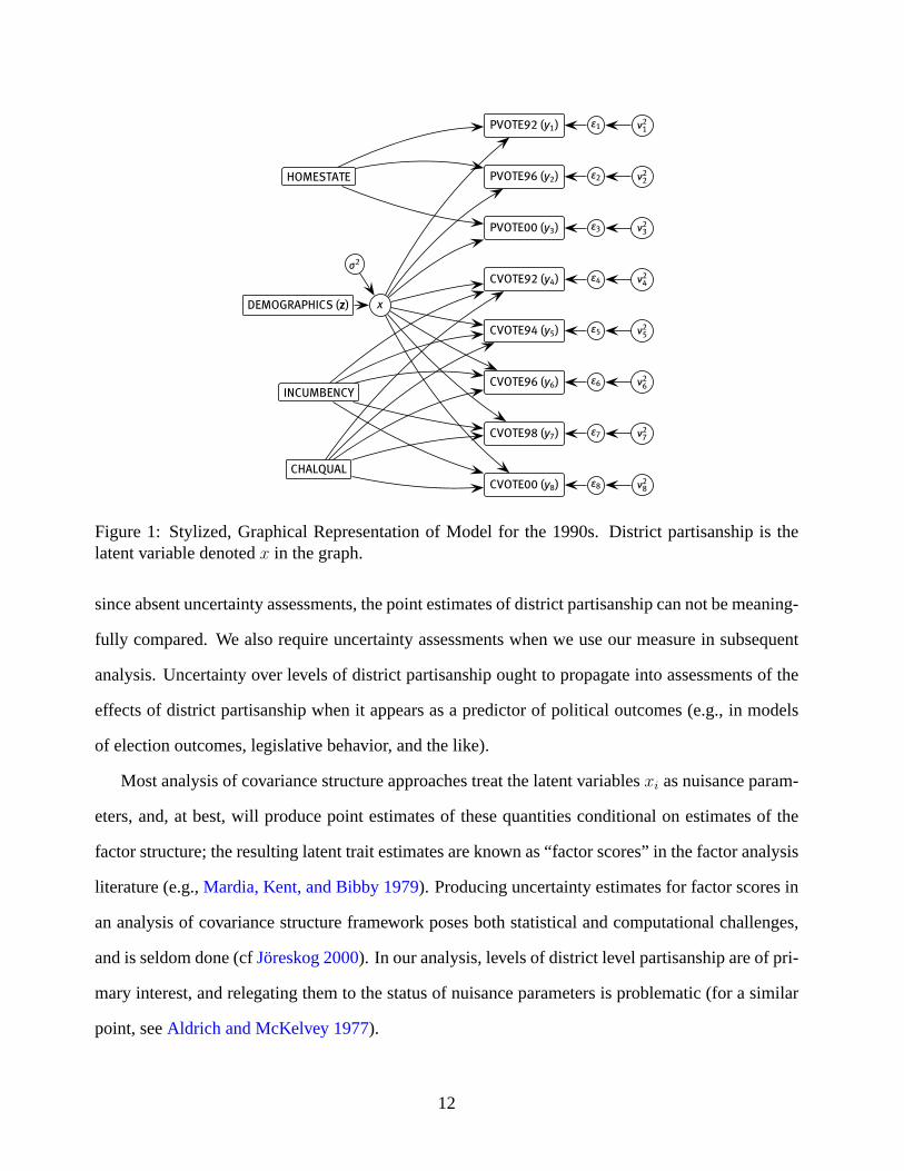
A stylized, graphical summary of the model appears in Figure 1, using the convention that unob-
served quantities appear in circles, and observed quantities appear in rectangles. Election outcomes
are akin to multiple indicators of district partisanship, xi, and treated as conditionally independent of
each other given xi and other predictors. In particular, note that we (1) augment the models for the
various presidential and congressional election outcomes (equations 2 through 5) with politically
relevant covariates (e.g., indicators for incumbency, challenger quality, region, home-state effects
and election-specific fixed effects) and (2) exploit the information in census aggregates about dis-
trict partisanship via equation 1. As Figure 1 demonstrates, demographic characteristics give rise to
district partisanship, and then that district partisanship is used to model the election outcomes.8
Bayesian Estimation and Inference
Our model is a structural equations model (SEM), as they are known in psychometrics. While
many political scientists are most familiar with estimation of these models using covariance struc-
ture methods — via software such as LISREL, AMOS, EQS — we adopt a Bayesian approach for
estimation and inference.
Advantages of a Bayesian Approach
First, a primary goal of our analysis is measurement: i.e., to produce estimates of district partisan-
ship, along with rigorous assessments of uncertainty (e.g., standard deviations, confidence intervals),
sional elections dataset and Scott Adler’s district demographic dataset; we treat a district as having
been redistricted when these data sources concur.8Another interpretation of the model is as a hierarchical or multilevel model (e.g., Hox 2002;
Skrondal and Rabe-Hesketh 2004); i.e., the latent district partisanship parameters, xi, are treated
here as similar to “random effects”, but with a “level 2” regression model (equation 1) exploiting
information about latent district partisanship in the time-invariant census aggregates, zi.
11
CVOTE00 (y8)
CVOTE98 (y7)
CVOTE96 (y6)
CVOTE94 (y5)
CVOTE92 (y4)
PVOTE00 (y3)
PVOTE96 (y2)
PVOTE92 (y1)
e8
e7
e6
e5
e4
e3
e2
e1
m28
m27
m26
m25
m24
m23
m22
m21
CHALQUAL
INCUMBENCY
HOMESTATE
xDEMOGRAPHICS (z)
r2
Figure 1: Stylized, Graphical Representation of Model for the 1990s. District partisanship is the
latent variable denoted x in the graph.
since absent uncertainty assessments, the point estimates of district partisanship can not be meaning-
fully compared. We also require uncertainty assessments when we use our measure in subsequent
analysis. Uncertainty over levels of district partisanship ought to propagate into assessments of the
effects of district partisanship when it appears as a predictor of political outcomes (e.g., in models
of election outcomes, legislative behavior, and the like).
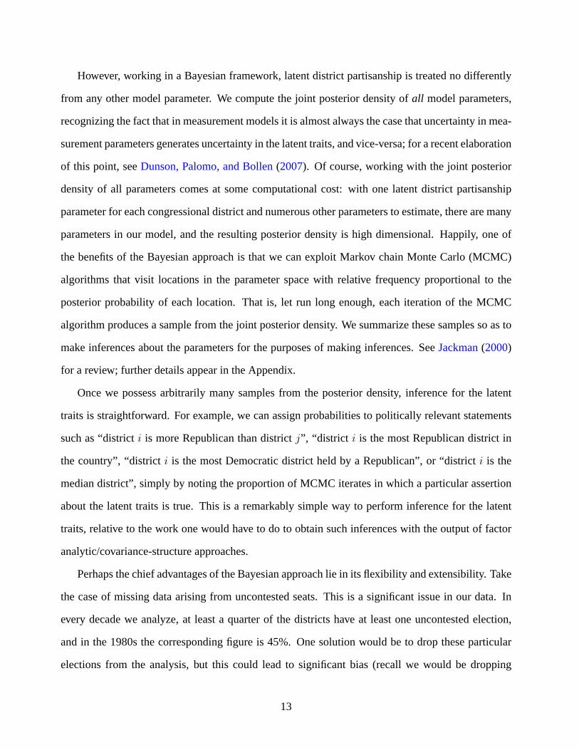
Most analysis of covariance structure approaches treat the latent variables xi as nuisance param-
eters, and, at best, will produce point estimates of these quantities conditional on estimates of the
factor structure; the resulting latent trait estimates are known as “factor scores” in the factor analysis
literature (e.g., Mardia, Kent, and Bibby 1979). Producing uncertainty estimates for factor scores in
an analysis of covariance structure framework poses both statistical and computational challenges,
and is seldom done (cf Joreskog 2000). In our analysis, levels of district level partisanship are of pri-
mary interest, and relegating them to the status of nuisance parameters is problematic (for a similar
point, see Aldrich and McKelvey 1977).
12
However, working in a Bayesian framework, latent district partisanship is treated no differently
from any other model parameter. We compute the joint posterior density of all model parameters,
recognizing the fact that in measurement models it is almost always the case that uncertainty in mea-
surement parameters generates uncertainty in the latent traits, and vice-versa; for a recent elaboration
of this point, see Dunson, Palomo, and Bollen (2007). Of course, working with the joint posterior
density of all parameters comes at some computational cost: with one latent district partisanship
parameter for each congressional district and numerous other parameters to estimate, there are many
parameters in our model, and the resulting posterior density is high dimensional. Happily, one of
the benefits of the Bayesian approach is that we can exploit Markov chain Monte Carlo (MCMC)
algorithms that visit locations in the parameter space with relative frequency proportional to the
posterior probability of each location. That is, let run long enough, each iteration of the MCMC
algorithm produces a sample from the joint posterior density. We summarize these samples so as to
make inferences about the parameters for the purposes of making inferences. See Jackman (2000)
for a review; further details appear in the Appendix.
Once we possess arbitrarily many samples from the posterior density, inference for the latent
traits is straightforward. For example, we can assign probabilities to politically relevant statements
such as “district i is more Republican than district j”, “district i is the most Republican district in
the country”, “district i is the most Democratic district held by a Republican”, or “district i is the
median district”, simply by noting the proportion of MCMC iterates in which a particular assertion
about the latent traits is true. This is a remarkably simple way to perform inference for the latent
traits, relative to the work one would have to do to obtain such inferences with the output of factor
analytic/covariance-structure approaches.
Perhaps the chief advantages of the Bayesian approach lie in its flexibility and extensibility. Take
the case of missing data arising from uncontested seats. This is a significant issue in our data. In
every decade we analyze, at least a quarter of the districts have at least one uncontested election,
and in the 1980s the corresponding figure is 45%. One solution would be to drop these particular
elections from the analysis, but this could lead to significant bias (recall we would be dropping
13

more than a quarter of the sample). This data is not missing at random, so standard imputation
techniques are inappropriate here. Indeed, the fact that an incumbent was reelected unopposed is
informative about underlying district partisanship. We model uncontested elections as censored
data, an approach used by Katz and King (1999) in their analysis of British House of Commons
election returns. That is, if a Democrat incumbent successfully runs unopposed then we model the
unobsered vote share via equation 2, subject to the constraint that the two-party Democratic vote
share is greater than 50% (i.e., that yij > .5 ⇐⇒ y∗ij > 0) ensuring that uncontestedness is
contributing some information about district partisanship. This constraint is trivial to implement
with our latent variable model. Imposing this (or any other non-standard) restriction in an analysis
of covariance model is extremely difficult, if not impossible. In an analysis of covariance model, to
the best of our knowledge, one would have to settle for either list-wise deletion or imputation based
on missing at random techniques, both of which are inappropriate here.9
Priors Densities over Parameters
In any Bayesian analysis it is incumbent on the researcher to report what prior densities are em-
ployed. Recall that we impose the identifying restriction that the latent xi have mean zero and vari-
ance one. With this restriction the model parameters are identified and we use vague priors, letting
the data dominate inferences for these parameters: i.e., a priori we specify independent N(0, 102)
priors for the regression parameters γ and β and vague inverse-Gamma priors for the variance param-
eters. With these normal and inverse-Gamma priors, and the normal distributions assumed for the
hierarchical structure over the latent district partisanship (equation 1) and the observed vote shares
(equations 2 and 4), the resulting posterior densities for the all model parameters are in the same
family as their prior (normals and inverse-gammas), ensuring that the computation for this problem
is rather simple (a case of conjugate Bayesian analysis); see the Appendix for further details.
9As an additional robustness check, we have also re-estimated our model using both an uncon-
strained imputation technique (e.g., imputations without the constraint), and treating election out-
comes in uncontested seats as missing at random. The substantive results generally remain similar.
14
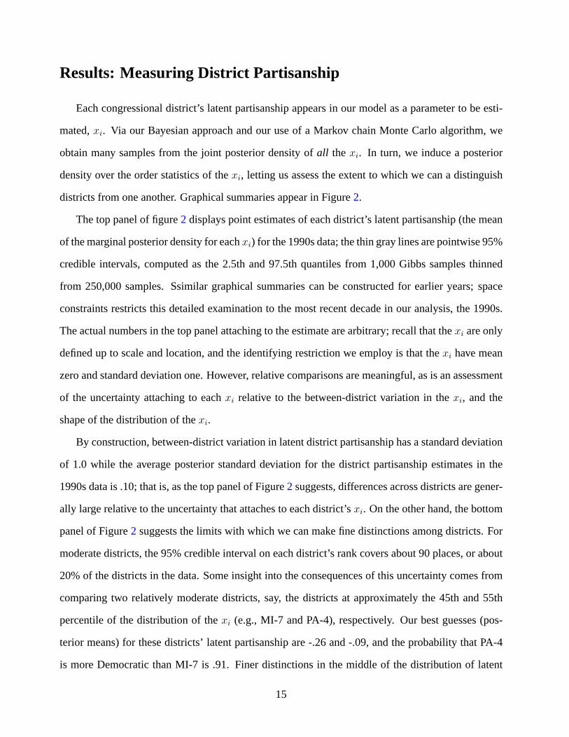
Results: Measuring District Partisanship
Each congressional district’s latent partisanship appears in our model as a parameter to be esti-
mated, xi. Via our Bayesian approach and our use of a Markov chain Monte Carlo algorithm, we
obtain many samples from the joint posterior density of all the xi. In turn, we induce a posterior
density over the order statistics of the xi, letting us assess the extent to which we can a distinguish
districts from one another. Graphical summaries appear in Figure 2.
The top panel of figure 2 displays point estimates of each district’s latent partisanship (the mean
of the marginal posterior density for each xi) for the 1990s data; the thin gray lines are pointwise 95%
credible intervals, computed as the 2.5th and 97.5th quantiles from 1,000 Gibbs samples thinned
from 250,000 samples. Ssimilar graphical summaries can be constructed for earlier years; space
constraints restricts this detailed examination to the most recent decade in our analysis, the 1990s.
The actual numbers in the top panel attaching to the estimate are arbitrary; recall that the xi are only
defined up to scale and location, and the identifying restriction we employ is that the xi have mean
zero and standard deviation one. However, relative comparisons are meaningful, as is an assessment
of the uncertainty attaching to each xi relative to the between-district variation in the xi, and the
shape of the distribution of the xi.
By construction, between-district variation in latent district partisanship has a standard deviation
of 1.0 while the average posterior standard deviation for the district partisanship estimates in the
1990s data is .10; that is, as the top panel of Figure 2 suggests, differences across districts are gener-
ally large relative to the uncertainty that attaches to each district’s xi. On the other hand, the bottom
panel of Figure 2 suggests the limits with which we can make fine distinctions among districts. For
moderate districts, the 95% credible interval on each district’s rank covers about 90 places, or about
20% of the districts in the data. Some insight into the consequences of this uncertainty comes from
comparing two relatively moderate districts, say, the districts at approximately the 45th and 55th
percentile of the distribution of the xi (e.g., MI-7 and PA-4), respectively. Our best guesses (pos-
terior means) for these districts’ latent partisanship are -.26 and -.09, and the probability that PA-4
is more Democratic than MI-7 is .91. Finer distinctions in the middle of the distribution of latent
15
RANK ORDER
DIS
TR
ICT
PA
RT
ISA
NS
HIP
1 50 100 150 200 250 300 350 400 450
−2
−1
0
1
2
3
4
−2
−1
0
1
2
3
4
10 MOST DEMOCRATIC:476: NY 16 (4.3)475: NY 15 (4.0)474: NY 11 (3.7)473: NY 10 (3.7)472: MI 15 (3.0)471: PA 2 (3.0)470: MI 14 (3.0)469: IL 2 (3.0)468: IL 1 (3.0)467: CA 35 (2.9)
10 MOST REPUBLICAN:10: NE 3 (−1.6)9: IN 6 (−1.6)8: TX 7, 1996−2000 (−1.7)7: AL 6 (−1.7)6: TX 26, 1992−1994 (−1.7)5: TX 3, 1992−1994 (−1.7)4: TX 8, 1996−2000 (−1.8)3: TX 8, 1992−1994 (−1.9)2: TX 7, 1992−1994 (−1.9)1: TX 19 (−1.9)
DISTRICTS IN SOUTHERN STATESDISTRICTS IN NON−SOUTHERN STATES
RANK ORDER
DIS
TR
ICT
PA
RT
ISA
NS
HIP
, OR
DE
R S
TA
TIS
TIC
1 50 100 150 200 250 300 350 400 450
0
100
200
300
400
0
100
200
300
400
Figure 2: Latent District Partisanship, 1990s: Pointwise Means and 95% Credible Intervals (top
panel), Order Statistics and 95% Credible Intervals (bottom panel).
16

district partisanship are made with less certainty, and will fall short of traditional standards used in
hypothesis testing. On the other hand, in the tails of the distribution, fine distinctions can be made
more readily: for instance, the probability that a district at the 1st percentile (e.g., AL 6) is more
Republican than a district at the 3rd percentile (e.g., KS 1) is greater than .99.
Additionally, Figure 2 shows the effect of redistricting and uncontestedness: both increase our
uncertainty of the district’s partisanship. Notice that some districts in have much wider credible
intervals than others, reflecting the increased uncertainty stemming from having fewer elections
contributing data for those districts.
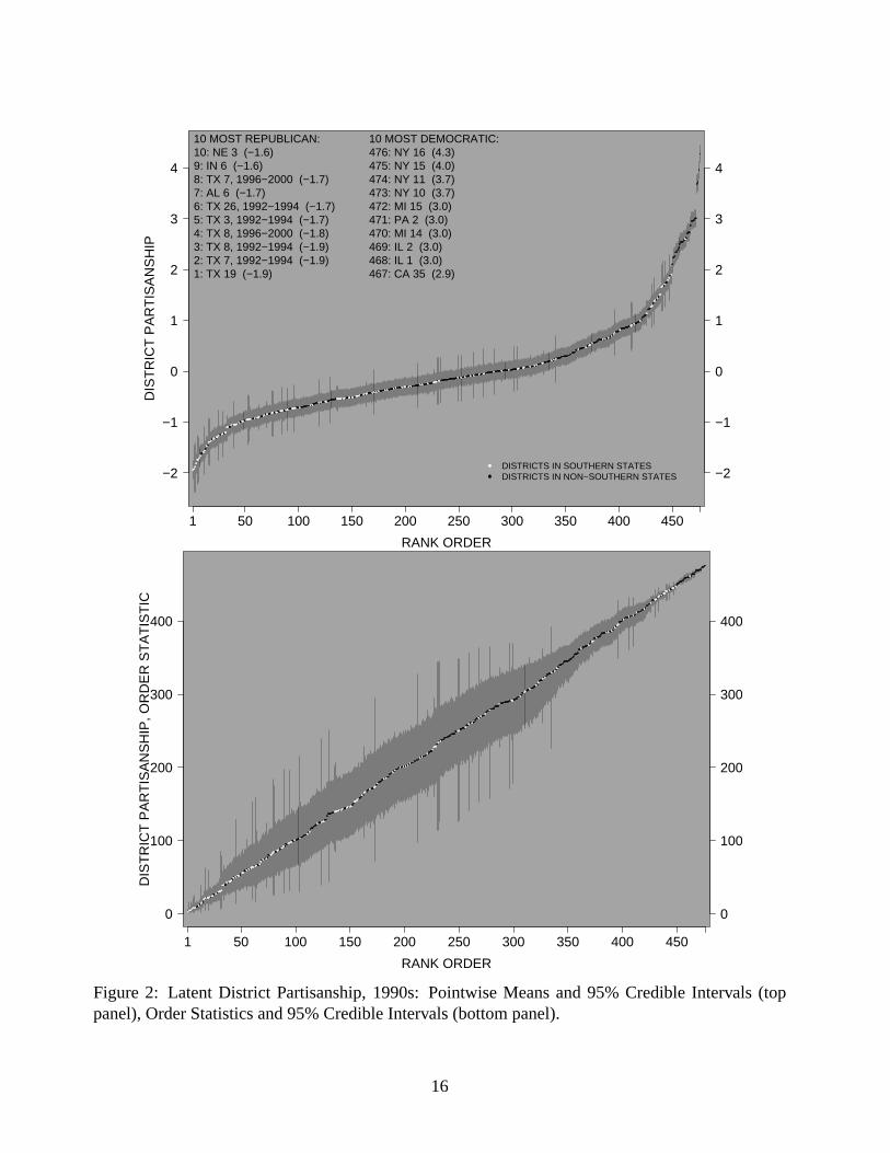
The distribution of latent district partisanship has a pronounced right-hand skew. The most
Democratic districts are roughly four standard deviations away from the mean district (set to zero, by
construction). On the other hand, the most Republican districts in the country are just two standard
deviations away from the mean. Quite simply, the most Democratic districts in our data exhibit
more consistent and more heavily Democratic voting patterns than the Republican districts exhibit
extreme pro-Republican voting patterns. For instance, in the ten most Democratic districts, Clinton
averaged 89% of the two party vote share in 1992 and 1996; in the ten most conservative districts,
Clinton averaged 30%, while in the remaining districts, Clinton averaged 54%.
Figure 3 shows the densities (smoothed histograms) of our district partisanship estimates in each
of the five decades we study. In each decade district partisanship is normalized to have a mean
of zero and unit variance across districts, so these graphs are not informative about any long term
trends in average levels of district partisanship (e.g., say, if the country, on average, was trending in
a particular partisan direction), or increases in the dispersion of district partisanship (e.g., as might
arise if redistricting was a source of partisan polarization, via the creation of lop-sided districts etc).
Nonetheless, the densities in Figure 3 do illustrate the way that district partisanship consistently has
a skewed distribution, and ways in which that skew has changed over time, reflecting both population
movements and redistricting. Specifically, in every decade we examine, there are a relatively small
number of extremely Democratic districts, without an offsetting set of extremely Republican districts.
This Democratic skew in the distribution of district partisanship is at its least pronounced in the first
17
1950s
District Partisanship (Posterior Means)
−2 0 2 4 6
1960s
District Partisanship (Posterior Means)
−2 0 2 4 6
1970s
District Partisanship (Posterior Means)
−2 0 2 4 6
1980s
District Partisanship (Posterior Means)
−2 0 2 4 6
1990s
District Partisanship (Posterior Means)
−2 0 2 4 6
Figure 3: Density plots of district partisanship estimates (means of marginal posterior densities),
by decade; higher values of district partisanship indicate more Democratic districts. Recall that for
each decade, the district partisanship estimates are recovered subject to the identifying restriction
that they have mean zero and unit variance across districts.
18

decade we analyze, the 1950s, and reaches its peak in the 1980s, where IL-1 (located on Chicago’s
south side) lies six standard deviations away from the average district.
More generally, the overwhelmingly Democratic districts in recent decades are almost all majority-
minority districts. Unsurprisingly, and as we elaborate below, the racial composition of a district is a
powerful determinant of its partisanship (see Table 1). For instance, the most Democratic district in
our analysis of the 1990s is NY 16 (centered on the South Bronx in New York City), whose popula-
tion in the 1990 Census was reported as 59% Hispanic origin and 43% black (these categories are not
mutually exclusive); Barone and Ujifusa (1995, 946) state that “[p]olitically ... [NY 16] ... is quite
possibly the most heavily Democratic district in the country.” The adjoining seat, NY 15 (centered
in Harlem), is the 2nd most Democratic seat in our analysis of the 1990s; it has been held by Charlie
Rangel since 1970, and was 47% black and 45% Hispanic origin in the 1990 Census. NY 10 and
NY 11, both in Brooklyn, are the 3rd and 4th most Democratic seats in our analysis, with black pop-
ulations of 60% and 75%, respectively. Districts in central Philadelphia (PA-2, 62% black), central
Detroit (MI-15, 70% black; MI-14, 69% black), the south side of Chicago (IL-1, 70% black; IL-2,
68% black) and South Central Los Angeles (CA-35, 43% black and 42% Hispanic origin) round
out the ten most Democratic districts in the 1990s. The correlation between the percentage of the
district’s population that is African-American and our measure of district partisanship is .60 in the
1990s.
Validating the District Partisanship Measure
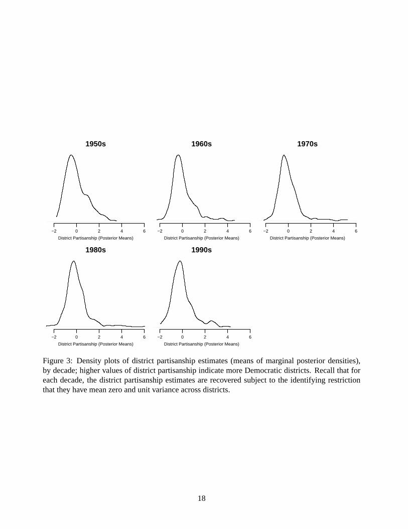
Figure 4 shows a scatterplot of the recovered latent trait and its indicators (presidential and
congressional vote shares) for the 1990s; similar plots for other decades are provided in the on-line
Appendix. The relationship between the vote shares and the latent trait is fairly strong, given that our
model treats vote shares as an indicator of the latent district partisanship. The non-linearities follow
from using log-odds transformations of the vote shares as indicators of latent district partisanship
(equations 2 and 4). Outliers are generally more prevalent in the congressional elections scatterplots,
resulting from the fact that congressional elections outcomes are modeled not only as a function
19

of latent district partisanship, but also with offsets for incumbency, challenger quality and region
(south/non-south).
A more realistic assessment of both the validity and usefulness of our measure of district partisan-
ship comes from seeing how well it predicts political outcomes not in our model, but still plausibly
related to district partisanship. The criterion variable we use is legislative preferences, as revealed via
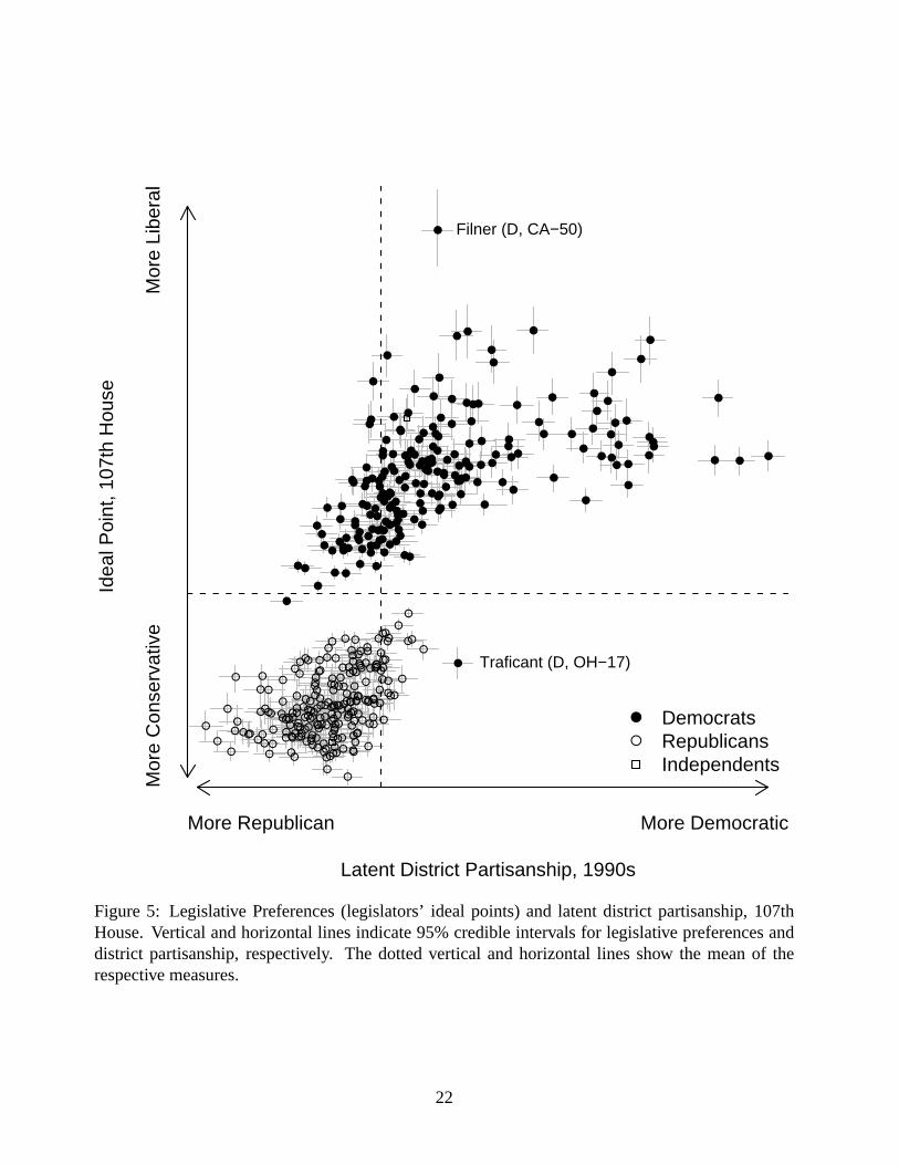
roll call voting. Figure 5 presents a scatterplot of legislative preferences (“ideal points”) against our
measure of district partisanship for the 1990s (again, see the appendix for similar displays from other
decades). The legislative ideal points are generated with a one dimensional spatial voting model fit
to all non-unanimous roll calls cast in the 107th U.S. House of Representatives (2001-2002), using
the model and estimation procedures described in Clinton, Jackman, and Rivers (2004). Where a
district was represented by more than one legislator over the course of the 107th Congress (e.g., due
to deaths and retirements), we display the ideal point of the legislator with the lengthier voting his-
tory. Both legislative ideal points and district partisanship are estimated with uncertainty, indicated
with the vertical and horizontal lines covering 95% credible intervals, respectively.
In general, there is a strong relationship between district partisanship and legislative ideal points;
the correlation between the two sets of point estimates is 0.73. The within-party correlations are also
moderate to large: 0.47 among Republicans, and 0.52 among Democrats. We would not expect a
perfect or even near-perfect relationship between district partisanship and a measure of legislators’
preferences, since there are many plausible sources of influence on roll-call voting other than district
partisanship, with party-specific whipping perhaps the most prominent. Indeed, perhaps the most
noteworthy feature of Figure 5 is the separation of legislators’ ideal points by party; there is almost
no partisan overlap in the estimated ideal points, while there is considerable overlap in estimates of
district partisanship across the two parties. No scholar of contemporary American politics would be
surprised by this finding, although a lively debate continues as to the sources of polarization within
the Congress (e.g., McCarty, Poole, and Rosenthal 2003). The pattern in Figure 5 is consistent
with a party pressure hypothesis (e.g., Snyder and Groseclose 2000), or a more general process
of polarization among political elites, showing that there is virtually no overlap between the ideal
20
−2
−1
01
23
4
0.2
0.4
0.6
0.8
1.0
Late
nt D
istr
ict P
artis
ansh
ip
Democratic Presidential Vote
●
●
●
●
●
●
●●
● ●
●
●
●●
●
●
●
●
●
●
● ●●
●
●
● ● ●
●
●
●
●
●
●
●
●
●
●●
●●
●
●
●
●
●
●●
●
●
●
●
●
●
●
●
●
●
●●●
●
●
●
●●
●
●
●
●
●●
●●
●
●
●
●
●
● ●
●
●
● ●
●
●
●
●
● ●
●
●
●
●
●
●
●
●
●
●
●●
●
●
●
●
●●
●
●●
●
●
●
●
●●
●
●
●●
●
●
●●
●
●
●
●
●
●
●●
●
●
●
●
●
●
●
●
●
●
●
●
●●
●
●
●
●
●
●●
●
●
●
●
●
●
●
●
● ●●
●
●
●
●●
●
●●●
●
●
●
●
●
●
●
●
●
●
●
●
● ●
● ●
●
●
●
●
●
●
●
● ●
●●
●
●
●
●
●
●
●
●●
●
●
●
● ●
●
●
●
●●
● ●
●
●
●
●
●
●
●
●
●
●
●
●
●
●
●
●
●
●
●
●
●
●
●
●
●
●
●
●
●
●●
●
●
●●
●
●
●
●
●●
●
●
●
●
●
●
●
●
●
●
●
●
●
●
●
●
●●
●
●
●
●
●
●●
●
●
●
●
●
●
●
●
●
●●●
●
●
●
●
●
●
●
●
●
●●
●
●●
●
●
●
●
●
●
●●
●● ●
●
●
●
●
●
●
●
●
●
●
●
●
● ●
●
● ●
●●
●●
●
●
●
●
●
●
●
●
●
●
●
●
●
●
●●
●●
●
●
●
●
●
●
●
●
●
●
●
●
●
●
●●
●
●
●
●●
●●
●
●
●
●●
●
●
●
●
●
●
●
●
●
●●
●
●
●
●
●●
●●
●
●
●
●
●
●
●
●●
●
●
●●
●
●
●
●
●
●
●
●
●
●
1992
Pre
side
ntia
l Vot
e
● ●
Non
−S
outh
ern
Dis
tric
tsS
outh
ern
Dis
tric
ts
−2
−1
01
23
4
0.2
0.4
0.6
0.8
1.0
Late
nt D
istr
ict P
artis
ansh
ip
Democratic Presidential Vote
●
●●
●●
●
●●
● ●
●
●
●●
●
●
●
●
●
●
● ●
●
●
●
● ●●
●
●
●
●
●
●
●
●
●
●
●
●
●
●
●
●
●
●
●●
●
●
●
●●
●
●
●
●
●
●●
●●
●
●
●●
●
●
●
●
●
●
●●
●●
●
●
●
●●
●
●
● ●
●
●
●●
● ●
●
●
●
●
●
●
●
●
●
●
●●
●
●
●
●
● ●
●
●●
●●
●
●
●●
●
●
●
●
●
●
●●
●
●
●
●
●
●
● ●
●
●
●
●
●
●
●
●
●
●
●
●
●
●
●
●
●
●
●●
●
●
●
●
●
●
●
●
●
● ●
●
●
●
●
●●
●
●
● ●
●
●
●
●
●
●
●
●
●
●
●
●
● ●
● ●
●
●●
●
●
●
●
● ●
●
●
●
●
●
●
●
●
●
● ●
●
●
●
● ●
●
●
●
●●
● ●
●
●
●
●
●
●
●
●
●
●
●
●●
●
●
●
●
●
●
●
●
●
●
●
●
●●
●
●
●●
●
●
●
●
●
●
●
●
●
●
●
●
●
●
●
●
●
●
●●
●
●
●
●
●
●
●
●
●
●●
●
●
●
●
●
●
●
●
●
●
●
●●
●
●●
●
●
●
●
●
●
●
●
●
●
●
●
●
●
●
●
●
●
●
●
●
●
●● ●
●
●
●
●
●
●
●
●
●
●
●
●
● ●
●
● ●
● ●
●
●
●
●
●
●
●
●
●
●
●
●
●
●
●
●
●
●
●
●
● ●
●
●●
●●
●
●
●
●
●
●
●
●
●
●
●
●
●●
●
●
●
●
●
●●
●
●
●
●●
●
●
●
●
●●
●
●
●
●
●
●
●
●
●
●
●
●
●
●
●
●
●
●
●
● ●
●
●
●
●●
●
●
●
●
●
1996
Pre
side
ntia
l Vot
e
−2
−1
01
23
4
0.2
0.4
0.6
0.8
1.0
Late
nt D
istr
ict P
artis
ansh
ip
Democratic Presidential Vote
●
●
●
●
●
●●
●
● ●●
●
●●
●
●
●
●
●
●
● ●
●●
●
● ● ●
●
●
●
●
●
●
●
●
●
●
●●
●
●
●
●
●
●
● ●
●
●
●
●●
●
●
●
●
●
●●
●
●●
●
●●
●
●
●
●
●
●
●
●
●●
●
●
●
●●
●
●
● ●
●
●
●
●
●●
●
●
●
●
●
●
●
●●
●
● ●
●●
●
●●●
●
●●
●
●
●
●
●●
●
●
●●
●
●
●●
●●
●●
●
●
● ●
●
●
●
●
●
●●
●
●
●●
●
●●
●
●
●
●
●
●●
●
●
●
●
●
●
●
●
● ●
●●
●
●
●●
●
●
●●
●
●
●
●
●
●
●
●
●
●
●
●
●●
●●
●
●
●
●
●
●
●
●●
●
●
●
●
●
●
●
●
●
● ●
●
●
●
●●
●
●
●
●
●
● ●
●
●
●
●
●
●
●●
●
●
●
●
●
●
●
●
●
●
●
●
●
●
●
●
●
●
●
●
●
●●
●
●
●
●
●
●
●
●
●
●
●
●
●
●
●
●
●
●
●●
●
●
●
●
●
●
●
●
●
●
●
●
●
●
●
●
●
●●
●
●
●
●●
●
● ●
●
●
●
●
●
●
●
●
●
●
●
●
●
●●
●
●
●
●
●
●
●
● ●●
●
●
●
●
●
●
●
●
●
●
●
●
●●
●
● ●
●●
●
●
●
●
●
●
●
●
●
●
●
●
●
●
●
●
●
●
●
●
● ●
●
●●
●
●●
●
●
●
●
●
●
●
●
●
●●
●
●
●
●
●
●
●●
●●
●
●
●●
●
●
●
●●
●
●
●
●
●
●
●
●
●
●
●
●
●
●
●
●
●●
●
●
●●
●
●●
●●
●
●
●
●
●
2000
Pre
side
ntia
l Vot
e
−2
−1
01
23
4
0.2
0.4
0.6
0.8
1.0
Late
nt D
istr
ict P
artis
ansh
ip
Democratic Congressional Vote
●
●
●
●
●
●
●
●
●●
●
●
● ●
●●
●
●
●
●●
●
●
●
● ● ●
●
●
●
●
●
●
●
●
●
●
●●
●
●
●
●
●
●
●
●
●
●
●
●
●
●
● ●
●
●
●
●
●●
●
●
●
●
●
●
●
●
●
● ●
●
●
● ●
●
●
●
●
●●
●
●
●
●
●
●
●
●
●
●
●●
●
●
●
●
● ●
●
● ●
●
●
●
●
●
●
●
●
●●
●
●
●
●
●●
●
●●
● ●
●
●
●
●
●
●
●
●
●
●
●
●
●
●
●
●
●
●
●
●
●
●
●
●
●
●●
●●●
●
●
●
●
●
●
● ●
●
●
●
●
●●
●
●
●
●
●
●●●
●●
●
●
●
●●
●
●
●●
●
●
●●
●
●
●
●
●
●●
●
●
●
●
●
●
●
●
●●●
●
●
●
●
●
●
●
●
●
●
●
●
●
●
●
●
●
●
●
●
●
●
●
●
●
●
●
●●
●
●
●
●●
●
●
●
●
●
●
●
●
●
●
●
●●
●
●
●
●
●
●
●
●
●
●
●
●●
●
●●
●
●
●
●
●
●
●
●
●
●●●
●
●
●
●
●
●
●
●●
●
●
●
●●
●
●
●
●
●
●
●
●● ●
●
●
●
●
●●
●
●
●
●
●
●
● ●
●
●●
● ●●
●
●
●
●
●
●
●
●
●
●
●
●
●●
● ●
●
●
●
●
●
●
●
●
●●
●
●
●
●
●
●●
●
●
●
●
●
●
●
●
●●
●
●
●
●
●
●
●
●
●
●
●●
●
●
●
●
●
●
●
●
●
●
●
●
●
●
●
●
●
●
1992
Con
gres
sion
al V
ote
−2
−1
01
23
4
0.2
0.4
0.6
0.8
1.0
Late
nt D
istr
ict P
artis
ansh
ip
Democratic Congressional Vote
●
●
●
●
●
●
●
●
●
●
● ●
●●●
●
●
●●
●
●
●
● ● ●
●
●
●
●
●
●
●
●
●
●
●
●
●
●
●
●
●
● ●
●
●
●
●
●
●
●
● ●
●
●
●
●
●
●
●
●
●
●●
●
●●●
●
● ●
●
●
●
●●
●
●
●
●
●
●
●
●
●
●
●
●
● ●
●
●
●
●
● ●●
●●
●
●
●
●
●
●●
●
●●
●
●
●
●
●
●
●
●
●●
●●
●
●
●
●
●
●
●
●
●
●
●●
●
●
●
●●
●
●
●
●
●
●
●
●●
●
●
●
●
●
●
●
●
● ●
●
●
●●
●●
●
●
●
●
●
●
●●
●●
●
●
●
●
●
●
●
●●
●
●
●
●
●
●
●
●
●
●●
●
●
● ●●
●
●
●
●
●●
●
●
●
●●
●
●
●
●
●
●
●
●
●
●
●
●
●
●
●
●
●
●
●
●
●
●
●
●●
●●
●
●
●
●
●
●
●
●
●
●
●
●
●
●●
●
●
●
●
●
●
●●
●
●
●●
●
●
●
●
●
●
●
●
●
●
●
●
●●
●●●
●
●
●
●
●
●
●
●
●
●
●
●
●
●● ●
●
●
● ●
●
●
●
●
●
●
●
●
●●
●
●
●●
●
●
●
●
●
●
●
●
●
●
●
●
● ●
●
●
●
●
●●
●
●
●
●●
●●
●
●
●
●
●●
●
●
●
●
●
●
●
●
●
●●
●
●
●
●
●●
●
●
●
●
●
●
●
●
●
●
●●
●
●
●●
●
●
●
●
●
●
●
●
●
1994
Con
gres
sion
al V
ote
−2
−1
01
23
4
0.2
0.4
0.6
0.8
1.0
Late
nt D
istr
ict P
artis
ansh
ip
Democratic Congressional Vote
●
●
●
●
●
●
●
●
●●
●
●
●
●
●
●
●
●●
● ●
●
●
●
● ●●
●
●
●
●
●
●
●
●
●
●
●
●
●
●
●
●
●
●
● ●
●
●
●
●●
●
●
●
●
●
● ●
●
●
●
●
●
●
●
●
●●
●
●
●
●
●
●
●
●
●● ●
●
●
● ●
●
●
●
●
●
●
●
●
●
●
●
●
●
●
● ●
●
●
●
●
● ●
●
●●
●
●
●
●
●
●
●
●
●
●
●
●
●
●
●
●
●
●
●●
●●
●
●
●
●
●
●
●
●●
●
●
●
●
●
●
●●
●
●
●
●
●
●
●
●
●
●
●
●
● ●
●
●
●
●
●●
●●
● ●
●
●
●
●
●●
●
●
●
●●
●
●●
●●
●
●
●
●
●
●
●
●
●●
●
●
●
●
●
●
●
●●
●
●
●
●
●
●
●●
●●
●●
●
●
●
●
●
●
●●
●●
●
●
●
●
●
●
●
●
●
●
●
●
●
●
●
●
●
●
●●
●
●
●
●
●
●
●
●
●
●
●
●
●
●
●
●
●
●●
●
●
●
●
●
●
●
●
●
●●
●
●
●●
●
●
●●
●
●
●●
●
●
●●
●
●
●
●
●
●
●
●
●●
●
●
●
●
●
●
●
●
●●
●
●●●
●
●
●●
●
●
●
●●
●
●
● ●●
●●
● ●
●
●
●
●
●●
●
●
●
●
●
●
●●
●
●
●
●
●
●
●
●●
●
●
●
●
●
●
●
●
●
●
●
●
●
●
●
●
●
●●
●
●
●
●
●
●
●●
●
●
●
●
●
●
●
●
●
●
●
●
●
●
●
●
● ●
●
●
●
●●
●
●
●
●
●
1996
Con
gres
sion
al V
ote
−2
−1
01
23
4
0.2
0.4
0.6
0.8
1.0
Late
nt D
istr
ict P
artis
ansh
ip
Democratic Congressional Vote
●
●
●
●
●
●
●
●
●
●
● ●
●
●
●
●
●
●●
●
●
●
●● ●●
●
●
●●
●
●
●
●
●
●
●
●
●
●
●
●
● ●
●
●
●
●
●
●
●
●
●
●
●
●
●
●
●
●
●
●
●
●
●
●
●
●
●●
●● ●
●
●
●
●
●
●
●●
●
●
●
●●
●
●
●
● ●
●
●
● ●
●
●●
●●
●
●
●
●
●●
●
●
●
●
●
●
●
●
●
●
●
●●
●
●
●
●
●
●
●
●●
●
●
●
●
●●
●
●
●
●
●
●
●
●
●
●
●
●
●●
●
●
●
●
●
●
●
● ●
●
●
●
●●
●
●
●
●
●
●
●
●●
●●
●
●
●
●
●
●
●●
●●
●
●
●
●
●
●●
● ●●
●●
●
●
●
●●
● ●
●
●
●
●
●
●●
●●
●
●
●
●
●
●
●
●
●
●
●
●
●
●
●●
●
●
●
●●
●
●
●
●
●
●
●
●
●
●
●
●
●●
●
●
●
●
●
●
●
●
●
●●
●
●
●
●
●
●
●
●
●
●●
●
●
●
●
●
●
●
●
●
●
●
●●
●●●
●
●
●
●
●
●
●
●
●
●
●
●
●
●●
●
●
●
●
●
●
●
●
●
●
●
●
●
●
●●
●
●
●●
●
●
●
●
●
●
●
●
●
●
●
●●
●●
●
●
●●
●
●
●
1998
Con
gres
sion
al V
ote
−2
−1
01
23
4
0.2
0.4
0.6
0.8
1.0
Late
nt D
istr
ict P
artis
ansh
ip
Democratic Congressional Vote
●
●
●
●
●
●
●
●
●
●
●
●
●
●
●
●●
●
●
●
●● ●
●
●
●
●●
●
●
●
●
●
●
●
●
●
●
●
●
● ●
●
●
●
●●
●
●
●
●
●
● ●●
●
●
●
●
●
●
●
●
●
●
●
●
●●
●
● ●
●
● ●
●
●
●
●
●●
●
●
●
●
●
●
●
● ●
●
●
●
●
● ●
●
●●
●●
●
●
●
●
●●
●●
●
●
●
●
●
●
●
●
●●
●●
●
●
●
●
●
●
●●
●●
●
●
●●
●●
●
●
●
●
●
●
●
●
●
●
●●
●●
●
●
●●
●
●●
● ●
●
●
●
●
●
●
●
●
●
●
●
●
●●
●●
●
●
●
●
●
●
●
●●
●
●
●
●
●
●
●
●
●
●
●
●
●
●
●
●
●●
● ●
●
●
●●
●
●
●
●
●
●
●
●
●
●
●
●
●
●
●
●
●
●
●
●●
●
●
●
●●
●
●●
●
●
●
●
●
●
●
●
●
●
●
●●
●
●
●
●
●
●
●
●
●
●
●
●
●●
●
●
●●
●
●
●
●
●●
●●
●
●
●
●
●
●
●
●
●
●
●
●
● ●
●
●
●
●
●
●
●
●
●
●
●● ● ●●●
●
●
●
●
●
●
●
●
●
●
●
●
●
●
●●
●●
●
●
●
●
●
●
●
●
●
●
●●
●
●
●
●
●
●
●
●
●
●
●
●
●
●
●
●
●
●
●
●
●
●●
●●
●
●
●
●●
●
●
●
●
2000
Con
gres
sion
al V
ote
Fig
ure
4:
Vote
Shar
esplo
tted
agai
nst
Lat
ent
Dis
tric
tP
arti
sansh
ip,
1990s.
Pre
siden
tial
elec
tion
outc
om
esar
em
odel
edas
afu
nct
ion
of
the
late
nt
trai
tplu
sin
terc
ept
shif
tsfo
rhom
e-st
ate
effe
cts.
Sim
ilar
ly,
the
model
for
congre
ssio
nal
elec
tion
outc
om
esin
cludes
inte
rcep
t
shif
tsfo
rin
cum
ben
cy,re
gio
nan
dch
alle
nger
qual
ity.
21
Latent District Partisanship, 1990s
Idea
l Poi
nt, 1
07th
Hou
se
More DemocraticMore Republican
Mor
e C
onse
rvat
ive
Mor
e Li
bera
l
●
●
●
●
●
●
●
●
●
●
●
●
●
●●
●
●
●
●
●
●●
●
●
●
●●
●
●
●
● ●
●
●
●
●
●
●
●
●
● ●
●
●
● ●
●
●
●
●
●●
●
●
●
●
●
●
●
● ●
●
●
●
●
●●
● ●
●
●●
●
●●
●
●
●
●
●
●
●●
●
●
●
●
●
●
●
●
●
●
●
●
●
●
●
●
●
●
●
●
●
●
●
●
●
●
●
●
●●
●
●●
●
●
●
●
●
●
●
●
●●
●
●
●
● ●
●
●●
●
●
●
●
●
●
●
●
●
●
●
●
●
●
● ●
●
●
●
●
●
●
●
●
●
●
●
●
●
●
●
●
●●
●
●
●
●
●
●
●●
●
●
●
●
●
●
●
●
● ●
●
●
●●
●●
● ●
●
●●
●
●
●
●
●●
●
●
●
●
●
●
●
●
●
●
●
●
●
●
●●
●
●
●
●
●
●
● ●
●
●
●
●
●
●
●
●
●●●
●●
●
●●● ●
●
●
●
●
●●
●
●
●
●
●
●
●
●
●
●
●
●
● ●
●
●
●
●
●
●
●
●
●
●
●●
●
●
●
●
●
●
●●
●
●
●
●
●
● ●
●
●
●
●
●
●
●
●
●
●
●
●●
●
●
● ●●
●
●
●
●
●
●●
●
●
●
●
●
●
●●
●
●
●
●
●
●
●
●
●●
●
●
●
●
●
●
●
●
●
●●
●
●
●
●
●
●
●
●●
●
●
●
●
●
●
●
●
●
●
●
●
●
●
●
●
●
●
●
●
●
●
●
●
●
●
●
●
●
●
●
●●
●
●
●
●
●
●
●
●
●
●
●
●
●
●
●
●
●
●
●
●
●
●
●
●
●
●
●
●●
●
●
●
●
●
●
●
Traficant (D, OH−17)
Filner (D, CA−50)
●
●
DemocratsRepublicansIndependents
Figure 5: Legislative Preferences (legislators’ ideal points) and latent district partisanship, 107th
House. Vertical and horizontal lines indicate 95% credible intervals for legislative preferences and
district partisanship, respectively. The dotted vertical and horizontal lines show the mean of the
respective measures.
22

points by party, while there is considerable overlap in our estimates of district partisanship by party-
of-representative.Put differently, there is much more partisan polarization in the roll call voting than
in the corresponding estimates of district partisanship.
Further, suppose we break the distribution of district partisanship at its mean value of zero,
labelling districts to the left of this point “Republican” districts and districts to the right as “Demo-
cratic”. Figure 5 reveals that there are 28 Democrats and 6 Republicans (13% and 3% of their
respective caucuses) who represent districts that, by this criterion, should be represented by the
other party. What can we say about these districts? First, all but 2 of these districts were represented
by incumbents in the 107th Congress, many of them long-time incumbents. While most are still
serving in Congress, 9 of these 31 incumbents had been defeated by 2007, and nearly all of these
defeated members had their loss attributed to their fit with the district by sources like the Almanac of
American Politics (Barone and Cohen 2006, and henceforth, AAP). And of the members still serving,
when they retire, the seat is likely to change partisan hands. Take the case of Gene Taylor (D-MS):
the AAP argues that if he were to retire, “Republicans would have an excellent change to capture this
seat” (AAP, 957). Indeed, of the members who have retired (a number of them were strategic retire-
ments prompted by redistricting), in all but one case party control of the seat flipped (the exception
is Ted Strickland who retired to become governor of Ohio in 2006 and was replaced by Democrat
Charles Wilson; undoubtedly the corruption scandal in the Ohio Republican Party played a role).
Furthermore, nearly all of these members are described as being political moderates and mavericks
out of step with their national parties and more line with their districts. In fact, 80% of the members
with mis-matched seats are described by the AAP as “moderate,” “centrist,” “conservative Demo-
crat,” “straddles both parties,” and so forth. Indeed, Ralph Hall, one of the Democrats representing a
Republican district, switched parties in 2004. Of the handful of members described as more typical
partisans, nearly all of them are described by the AAP as focusing on the “grassroots” or other issues
important to their district, suggesting that they win by promoting service to the district. Taken as a
whole, this analysis suggests even more validity for our measure of district partisanship.
Since our main purpose is to measure and model district partisanship we defer a more detailed
23

analysis of representation or polarization for another day; a complete list of “mismatched” members
of Congress and their districts appears in the on-line Appendix. For now we simply note that the
the relationship between our measure of district partisanship and election returns is very strong (par-
ticularly in the 1990s) and that the correlation between district partisanship and estimated legislator
ideal points is consistent with our general expectations. This not only bolsters our confidence in the
measure, but demonstrates its usefulness for analyzing Congressional politics.
Social-structural correlates of district partisanship
Table 1 presents parameter estimates of the demographic component of the model (equation 1),
where latent district partisanship is modeled as a function of these census aggregates. Of the many
demographic variables aggregated to the level of congressional districts in the census, which ones
are more politically relevant than others? A long line of research with its roots in political sociology
suggests that indicators of social class ought to be relevant in this context: these include median
income or the composition of the workforce (e.g., unemployment rates, percent blue-collar, percent
unionized). In addition, studies of committee assignments have focused on the role that particular
demographic characteristics play in shaping the behavior of members of Congress. These studies
supply predictions about how we might expect constituent partisanship and demographic character-
istics to be related; a useful summary appears in Adler and Lapinski’s (1997) listing of politically-
relevant district characteristics in their study of demand for policy outputs from Congress.10
For the most part, the relationships we find between district partisanship and demographic char-
acteristics contain few surprises, as presented in Table 1. First, and as discussed previously, dis-
tricts with high proportions of African-Americans are consistently among the most Democratic dis-
tricts. Over the five decades in our analysis, the coefficient on the log of the proportion of African-
Americans in the population (outside of the South) is always unambiguously positive, and averages
about .10. In each decade, the distribution of African-Americans throughout congressional districts
10Moreover, the demographic variables we use come from Adler’s (2003) dataset on Congres-
sional district demographics.
24

1952-1960 1962-1970 1972-1980 1982-1990 1992-2000
Intercept 7.94 27.13 31.16 22.88 16.94
[3.96, 11.87] [20.17, 35.58] [21.67, 41.94] [17.90, 29.88] [13.17, 21.22]
Log Proportion Aged 65+ -0.71 -0.79 -0.40 0.038 0.47
[-1.07, -0.34] [-1.06, -0.53] [-0.67, -0.14] [-0.18, 0.26] [0.28, 0.65]
Log Proportion Blue Collar -0.24 0.33 0.24 -0.16 -0.071
[-0.58, 0.11] [-0.088, 0.74] [-0.085, 0.57] [-0.39, 0.077] [-0.26, 0.12]
Log Proportion Foreign Born -0.05 0.33 0.11 0.08 0.20
[-0.16, 0.05] [0.22, 0.44] [0.0069, 0.21] [-0.0075, 0.17] [0.13, 0.28]
Log Median Income -1.18 -2.62 -2.70 -1.88 -1.05
[-1.60, -0.72] [-3.14, -2.11] [-3.27, -2.12] [-2.23, -1.52] [-1.40, -0.68]
Log Population Density 0.14 0.17 0.27 0.19 0.22
[0.087, 0.20] [0.13, 0.21] [0.22, 0.32] [0.14, 0.23] [0.18, 0.26]
Log Proportion Unemployed 0.34 0.57 0.48 0.60 0.85
[0.10, 0.58] [0.28, 0.86] [0.19, 0.75] [0.37, 0.85] [0.59, 1.14]
Log Proportion Black 0.12 0.12 0.089 0.066 0.094
[0.045, 0.20] [0.058, 0.18] [0.022, 0.16] [0.0088, 0.12] [0.035, 0.15]
South (dummy) 0.49 -0.36 -0.14 -0.27 0.14
[0.0095, 0.98] [-0.87, 0.11] [-0.61, 0.28] [-0.62, 0.074] [-0.15, 0.43]
Log Proportion Black × South 0.23 0.12 0.0088 0.14 0.30
[0.043, 0.42] [-0.074, 0.32] [-0.17, 0.18] [0.0083, 0.27] [0.19, 0.40]
Majority-Minority - - - 2.05 0.93
[1.61, 2.47] [0.56, 1.31]
σx 0.75 0.70 0.69 0.56 0.50
[0.69, 0.80] [0.65, 0.75] [0.64, 0.73] [0.53, 0.61] [0.47, 0.54]
r2x 0.44 0.51 0.53 0.68 0.75
[0.36, 0.52] [0.43, 0.58] [0.46, 0.59] [0.63, 0.72] [0.71, 0.78]
Table 1: Posterior Summaries, Relationships Between Demographic Characteristics and Latent Dis-
trict Partisanship. Cell entries are posterior means; 95% credible intervals shown in brackets. Me-
dian income is median family income; population density is population per mile2; South is defined
as the 11 states of the former confederacy. See Adler (2003) for additional details.
25

is skewed to the right: i.e., the median African-American proportion is consistently around .10, but
attains a maximum of .92 in the 1980s (in IL 1), and .88 in the 1970s and 1960s, .74 in the 1990s (in
NY 11), and .69 in the 1950s (in MS 3), with an average 95th percentile of .42. Thus, in the 1990s, in
a non-Southern district, an increase in the proportion of the African-American population from the
mean level of .13 to .57 (the 95th percentile) is associated with an increase of district partisanship
of approximately 15% of a standard deviaton, net of other factors. Additionally, the coefficient for
majority-minority districts is large and statistically significant, indicating the even controlling for the
fact that majority-minority districts contain a high percentage of African-Americans, such districts
are even more Democratic.
Other variables that are also consistently and strongly associated with district partisanship are
median income and population density. Richer districts (as measured by the district’s median per
capita income) are consistently less Democratic than poorer districts. Our parameter estimates imply
that net of other factors, movement from the 5th to the 95th percentile on income is associated
with anywhere from a standard deviation’s worth of change in district partisanship (e.g., 1950s and
1990s), to 2.1 standard deviations of change in district partisanship in the 1960s. Population density
displays tremendous variation in any given decade; movement from the 5th is 95th percentile on this
variable is associated with shifting latent district partisanship a standard deviation (in a Democratic
direction) in the 1960s, but up to a two standard deviation shift in the 1970s. Overall, the main result
we stress from this section is the strong and sensible relationship between the demographics and our
district partisanship measure.
Congressional Elections
Estimates of the Congressional elections models appear in Tables 2 and 3. The models fit rea-
sonably well, with the r-squared values for the 25 equations ranging from a low of .65 in 1954 to
a high of .90 in 2000. The parameters tapping the effects of district partisanship range from a low
of .26 in 1972 to .62 in 1956. Recent House elections, say, 1994-2000, have been characterized
26

by (a) reasonably good model fit and (b) relatively high discrimination with respect to the latent
partisanship measure.
The estimates for the incumbency offset parameters are of some substantive interest. Since our
dependent variable in the vote equations is the log-odds ratio of vote shares, we implicitly have a non-
linear model in vote shares themselves; to simplify the assessment of the model’s marginal effects,
we assess all marginal effects conditional on vote shares being at 50%, corresponding to districts that
are otherwise evenly split between Democrats and Republicans (note that the 50-50 vote split is also
the steepest part of the logistic CDF, where marginal effects on votes take their maximum possible
value). In addition, our Congressional elections model includes terms for challenger quality (i.e., a
dummy variable coded 1 if the challenger has previously held elective office and zero otherwise).
Incumbency offsets are estimated separately for Northern and Southern states, and also for
Democratic and Republican incumbents. The regional variation in the magnitude of the incumbency
offsets is perhaps the most striking feature of this part of the results. For the 1950s, we estimate
massive incumbency offsets for Democratic incumbents in the South, worth anywhere from 10 to 20
percentage points of vote share in an otherwise evenly split district. Incumbency offsets for North-
ern Democrats and all Republicans in the 1950s are much smaller; in fact, for Southern Republicans
prior to the 1970s (when there are relatively few Southern Republican incumbents in the House),
our estimates of incumbency offsets are indistinguishable from zero at conventional levels of sta-
tistical significance. In general, there is no systematic pattern of incumbency offsets being larger
for one party than the other.11 There is some regional asymmetry, particularly on the Democratic
side, although this is concentrated primarily in the early part of our study. Although we stress we
are estimating a different quantity of interest, our results closely parallel the larger literature on the
incumbency advantage, which finds a substantial increase in the incumbency advantage in the 1960s
and 1970s, followed by modest decline in the late 1980s and 1990s.12
11Evidence of a partisan asymmetry would be when the 95% highest posterior density interval on
the sum of the Democratic incumbency offset and the (negatively-signed) Republican incumbency
offset does not overlap zero.12For example, see Alford and Brady (1993), Gelman and King (1990), and Ansolabehere, Snyder
27

Dis
tric
tD
emocr
atic
Rep
ubli
can
South×
Dem
South×
Rep
ub
Dem
Chal
lenger
Rep
Chal
lenger
Yea
rIn
terc
ept
Par
tisa
nsh
ipIn
cum
ben
cyIn
cum
ben
cyIn
cum
ben
cyIn
cum
ben
cyQ
ual
ity
Qual
ity
ν jr2
1952
0.0
53
0.5
00.0
77
-0.2
20.9
50.0
23
--
0.3
20.8
1[-
0.0
31
,0
.14
][0
.45
,0
.55
][-
0.0
43
,0
.19
][-
0.3
2,
-0.1
1]
[0.8
0,
1.0
9]
[-0
.46
,0
.47
][0
.29,
0.3
5]
[0.7
7,
0.8
4]
1954
0.6
50.5
8-0
.37
-0.5
80.9
90.0
6-
-0.5
20.6
5[0
.47
,0
.83
][0
.50
,0
.67
][-
0.5
9,
-0.1
5]
[-0
.78
,-0
.37
][0
.76
,1
.19
][-
0.3
6,
0.5
0]
[0.4
8,
0.5
7]
[0.5
9,
0.7
0]
1956
0.3
10.6
2-0
.22
-0.2
91.1
7-0
.022
0.0
23
0.1
20.5
50.6
5[0
.11
,0
.53
][0
.54
,0
.71
][-
0.4
8,
0.0
29
][-
0.5
1,
-0.0
52
][0
.95
,1
.40
][-
0.4
7,
0.4
1]
[-0
.16
,0.2
0]
[-0.1
1,
0.3
9]
[0.5
0,
0.5
9]
[0.5
9,
0.7
1]
1958
0.2
70.3
70.3
8-0
.28
0.8
7-0
.021
0.1
3-0
.13
0.2
90.8
0[0
.18
,0
.36
][0
.31
,0
.42
][0
.26
,0
.51
][-
0.3
9,
-0.1
7]
[0.7
0,
1.0
4]
[-0
.26
,0
.22
][0
.03
2,
0.2
3]
[-0
.26
,0.0
06
8]
[0.2
7,
0.3
2]
[0.7
7,
0.8
4]
1960
0.2
00.4
60.1
9-0
.23
0.7
3-0
.12
0.0
31
-0.0
75
0.4
00.7
3[0
.05
3,
0.3
3]
[0.3
9,
0.5
2]
[0.0
36
,0
.37
][-
0.4
0,
-0.0
66
][0
.58
,0
.89
][-
0.4
8,
0.2
3]
[-0
.13
,0.1
8]
[-0.2
1,
0.0
7]
[0.3
7,
0.4
3]
[0.6
8,
0.7
6]
1962
0.1
10.3
20.2
5-0
.40
0.4
80.1
5-
-0.2
90.7
9[0
.03
8,
0.1
9]
[0.2
8,
0.3
6]
[0.1
5,
0.3
4]
[-0
.49
,-0
.30
][0
.36
,0
.60
][-
0.1
4,
0.4
0]
[0.2
6,
0.3
2]
[0.7
5,
0.8
3]
1964
0.3
40.3
30.3
0-0
.40
0.1
00.0
76
0.0
91
-0.1
30.3
00.7
8[0
.25
,0
.43
][0
.29
,0
.38
][0
.19
,0
.40
][-
0.5
1,
-0.2
9]
[-0
.01
2,
0.2
1]
[-0
.13
,0
.28
][-
0.0
087
,0.1
9]
[-0.2
5,
-0.0
10]
[0.2
7,
0.3
2]
[0.7
4,
0.8
1]
1966
0.0
61
0.3
60.2
8-0
.57
0.3
20.1
50.0
44
-0.1
90.2
30.8
8[-
0.0
28
,0
.15
][0
.33
,0
.40
][0
.17
,0
.39
][-
0.6
7,
-0.4
5]
[0.2
1,
0.4
3]
[-0
.02
7,
0.3
1]
[-0.0
62
,0.1
5]
[-0.2
8,
-0.1
1]
[0.2
1,
0.2
6]
[0.8
5,
0.9
0]
1968
0.2
20.4
00.1
5-0
.67
0.4
60.0
82
0.1
5-0
.10
0.3
00.8
5[0
.12
,0
.32
][0
.36
,0
.45
][0
.01
7,
0.2
8]
[-0
.78
,-0
.55
][0
.33
,0
.59
][-
0.0
83
,0
.24
][0
.047
,0.2
6]
[-0.2
1,
0.0
12]
[0.2
7,
0.3
3]
[0.8
2,
0.8
7]
1970
0.1
00.3
70.5
1-0
.40
0.3
80.0
14
0.1
0-0
.11
0.3
10.8
3[0
.00
16
,0
.20
][0
.32
,0
.42
][0
.39
,0
.64
][-
0.5
1,
-0.2
7]
[0.2
4,
0.5
3]
[-0
.14
,0
.18
][-
0.0
17
,0.2
2]
[-0
.23
,0.0
12
][0
.29,
0.3
4]
[0.8
0,
0.8
6]
1972
0.0
80.2
60.5
9-0
.61
0.0
15
-0.2
60.2
0-0
.21
0.3
50.7
8[-
0.0
03
9,
0.1
7]
[0.2
2,
0.3
0]
[0.4
7,
0.7
0]
[-0
.73
,-0
.49
][-
0.1
3,
0.1
5]
[-0
.43
,-0
.09
9]
[0.0
59
,0.3
3]
[-0
.33
,-0
.091
][0
.33
,0.3
8]
[0.7
5,
0.8
1]
1974
0.4
00.3
20.4
3-0
.55
0.1
2-0
.18
0.1
8-0
.09
0.3
70.7
6[0
.29
,0
.51
][0
.27
,0
.37
][0
.31
,0
.57
][-
0.6
9,
-0.4
1]
[-0
.02
3,
0.2
6]
[-0
.32
,-0
.03
7]
[0.0
6,
0.2
9]
[-0
.27
,0.0
98
][0
.34,
0.4
0]
[0.7
2,
0.7
9]
Tab
le2:
Post
erio
rS
um
mar
ies,
Congre
ssio
nal
Ele
ctio
ns
Model
,1952-1
974.
Cel
len
trie
sar
epost
erio
rm
eans,
95%
cred
ible
inte
rval
sin
bra
cket
s.In
all
yea
rs,
the
dep
enden
tvar
iable
isth
elo
g-o
dds
of
the
Dem
ocr
atic
pro
port
ion
of
the
two-p
arty
vote
inco
nte
sted
House
race
s.S
eeeq
uat
ion
2.
Chal
lenger
qual
ity
dat
ais
not
avai
lable
inal
lyea
rs.
28
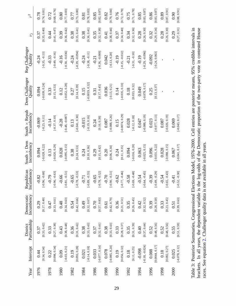
Dis
tric
tD
emocr
atic
Rep
ubli
can
South×
Dem
South×
Rep
ub
Dem
Chal
lenger
Rep
Chal
lenger
Yea
rIn
terc
ept
Par
tisa
nsh
ipIn
cum
ben
cyIn
cum
ben
cyIn
cum
ben
cyIn
cum
ben
cyQ
ual
ity
Qual
ity
ν jr2
1976
0.4
40.3
70.2
9-0
.82
0.0
94
-0.0
69
0.0
94
-0.2
40.3
70.7
8[0
.34
,0
.54
][0
.33
,0
.42
][0
.17
,0
.40
][-
0.9
6,
-0.6
8]
[-0
.02
8,
0.2
2]
[-0
.25
,0
.11
][-
0.0
39
,0.2
4]
[-0.3
5,
-0.1
3]
[0.3
5,
0.4
0]
[0.7
4,
0.8
1]
1978
0.2
20.3
30.4
7-0
.79
0.1
3-0
.14
0.3
3-0
.33
0.4
40.7
2[0
.09
8,
0.3
4]
[0.2
7,
0.3
8]
[0.3
3,
0.6
1]
[-0
.96
,-0
.63
][-
0.0
20
,0
.29
][-
0.3
7,
0.1
0]
[0.1
5,
0.5
3]
[-0.4
9,
-0.1
6]
[0.4
1,
0.4
7]
[0.6
8,
0.7
6]
1980
0.0
90.4
30.4
8-0
.66
0.0
28
-0.2
80.1
2-0
.16
0.3
90.8
0[-
0.0
3,
0.2
1]
[0.3
8,
0.4
8]
[0.3
4,
0.6
3]
[-0
.81
,-0
.51
][-
0.0
95
,0
.15
][-
0.4
8,
-0.0
87
][-
0.0
52
,0.2
8]
[-0
.30
,-0
.036
][0
.36
,0.4
2]
[0.7
7,
0.8
3]
1982
0.1
90.3
60.5
4-0
.65
0.3
80.1
30.2
7-0
.24
0.3
80.7
7[0
.09
3,
0.2
8]
[0.3
1,
0.4
2]
[0.4
2,
0.6
6]
[-0
.78
,-0
.53
][0
.24
,0
.53
][-
0.0
41
,0
.30
][0
.14,
0.3
9]
[-0
.39
,-0
.094
][0
.35
,0.4
1]
[0.7
3,
0.8
0]
1984
0.0
21
0.3
80.4
9-0
.71
0.2
4-0
.015
0.1
5-0
.24
0.3
80.8
1[-
0.1
4,
0.1
8]
[0.3
3,
0.4
3]
[0.3
2,
0.6
7]
[-0
.89
,-0
.55
][0
.10
,0
.36
][-
0.1
9,
0.1
6]
[-0.0
01
9,
0.3
2]
[-0.3
8,
-0.1
1]
[0.3
6,
0.4
1]
[0.7
8,
0.8
3]
1986
0.0
33
0.3
70.7
0-0
.65
0.2
90.2
40.3
1-0
.21
0.3
50.8
5[-
0.0
77
,0
.14
][0
.32
,0
.41
][0
.57
,0
.83
][-
0.7
8,
-0.5
2]
[0.1
5,
0.4
2]
[0.1
0,
0.3
9]
[0.1
7,
0.4
5]
[-0
.36
,-0
.069
][0
.32
,0.3
8]
[0.8
2,
0.8
7]
1988
0.0
78
0.3
80.6
1-0
.70
0.2
00.0
87
0.0
36
0.0
42
0.4
10.8
2[-
0.0
85
,0
.24
][0
.33
,0
.43
][0
.42
,0
.79
][-
0.9
0,
-0.5
1]
[0.0
6,
0.3
4]
[-0
.08
8,
0.2
6]
[-0.1
3,
0.2
1]
[-0
.13
,0.2
0]
[0.3
8,
0.4
4]
[0.7
9,
0.8
4]
1990
0.1
90.3
30.3
6-0
.62
0.2
40.1
50.1
4-0
.19
0.3
70.7
6[0
.05
6,
0.3
2]
[0.2
8,
0.3
7]
[0.2
1,
0.5
1]
[-0
.77
,-0
.46
][0
.11
,0
.35
][-
0.0
07
4,
0.2
9]
[-0
.03
5,
0.3
3]
[-0
.35
,-0
.032
][0
.34
,0.4
0]
[0.7
2,
0.7
9]
1992
0.1
80.3
50.3
5-0
.58
0.0
94
0.0
28
0.1
8-0
.21
0.3
40.7
5[0
.11
,0
.25
][0
.31
,0
.39
][0
.26
,0
.45
][-
0.6
9,
-0.4
8]
[-0
.01
6,
0.2
0]
[-0
.12
,0
.18
][0
.03
3,
0.3
2]
[-0
.31
,-0
.10]
[0.3
2,
0.3
6]
[0.7
1,
0.7
8]
1994
-0.0
98
0.4
00.4
2-0
.54
0.0
63
0.0
47
0.0
49
-0.1
90.2
80.8
5[-
0.1
8,
-0.0
24
][0
.37
,0
.44
][0
.32
,0
.52
][-
0.6
4,
-0.4
5]
[-0
.02
5,
0.1
5]
[-0
.08
8,
0.1
9]
[-0.0
78
,0.1
7]
[-0.2
9,
-0.0
96]
[0.2
6,
0.3
0]
[0.8
3,
0.8
7]
1996
0.0
88
0.5
20.3
9-0
.39
0.0
96
0.0
23
0.2
5-0
.092
0.3
20.8
6[0
.00
44
,0
.17
][0
.48
,0
.56
][0
.28
,0
.50
][-
0.4
9,
-0.2
9]
[-0
.03
1,
0.2
2]
[-0
.07
7,
0.1
3]
[0.1
3,
0.3
7]
[-0.2
4,
0.0
63]
[0.2
9,
0.3
4]
[0.8
3,
0.8
7]
1998
0.1
80.5
20.3
3-0
.54
0.0
28
0.0
87
--
0.2
80.8
9[0
.08
2,
0.2
7]
[0.4
8,
0.5
6]
[0.2
3,
0.4
5]
[-0
.65
,-0
.43
][-
0.0
88
,0
.15
][-
0.0
26
,0
.19
][0
.26,
0.3
0]
[0.8
7,
0.9
1]
2000
0.0
25
0.5
50.5
1-0
.41
0.0
67
0.0
69
--
0.2
90.9
0[-
0.0
78
,0
.12
][0
.51
,0
.59
][0
.39
,0
.63
][-
0.5
2,
-0.3
0]
[-0
.04
1,
0.1
7]
[-0
.04
3,
0.1
7]
[0.2
7,
0.3
1]
[0.8
8,
0.9
1]
Tab
le3:
Post
erio
rS
um
mar
ies,
Congre
ssio
nal
Ele
ctio
ns
Model
,1976-2
000.
Cel
len
trie
sar
epost
erio
rm
eans,
95%
cred
ible
inte
rval
sin
bra
cket
s.In
all
yea
rs,
the
dep
enden
tvar
iable
isth
elo
g-o
dds
of
the
Dem
ocr
atic
pro
port
ion
of
the
two-p
arty
vote
inco
nte
sted
House
race
s.S
eeeq
uat
ion
2.
Chal
lenger
qual
ity
dat
ais
not
avai
lable
inal
lyea
rs.
29

We also estimate challenger quality offsets, following the standard operationalization of a “qual-
ity” challenger being one who has previously won an election for public office (e.g., Jacobson and
Kernell 1983, 30). Our results indicate that quality challengers often – but certainly not always –
improve their party’s vote share. The 95% highest posterior density intervals for these offsets fre-
quently overlap zero (11 out of 20 times for Democrats; 8 out of 20 times for Republicans). But in a
typical year, the estimated offset for a quality Republican challenger in an otherwise evenly-poised
race is on the order of 3 to 4 percentage points of vote share, and roughly the same for a quality
Democrat. Large estimates of challenger quality are obtained for 1978, for both parties (roughly
corresponding to 7 to 8 percentage points), representing the approximate peak of a not-especially-
strong rise and fall in challenger quality offsets. We stress that these effects are small relative to the
incumbency offsets we estimate, but, nonetheless, large enough to be decisive in an otherwise close
race. We also stress that challenger quality is, no doubt, endogenous to district partisanship, with
districts heavily favoring Democratic candidates less likely to attract quality Republican candidates,
and vice-versa.
Presidential Elections
Results for our presidential elections models appear in Table 4. Two features stand out. First,
the relationship between latent district partisanship and presidential elections outcomes has become
considerably stronger over time; the discrimination parameter for district partisanship ranges from
a low of .32 in 1964 to a maximum of .67 in 2000, with higher value appearing in the 1980s and
1990s.13 In addition, the r2 for the presidential elections model generally increases over time, largely
and Stewart (2001).13The term “discrimination” parameter comes from the educational testing literature, where a test
item helps us discriminate among test-subjects of higher and lower abilities; analogously, elections
differ in the extent to which they convey information about varying levels of partisanship. The iden-
tifying restriction that district partisanship has mean zero and standard deviation one across districts
within any given decade allows us to make these over-time comparisons about the discrimination
30

following the rise of the discrimination parameters, reaching levels above .90 for the 1976-2000
period. Taken together, this is evidence of the increasing partisan character of elections; in turn,
this reflects the fact that at least at the district level, presidential election outcomes are more highly
correlated with one another across successive elections, and with the outcomes of congressional
elections.
Individual presidential elections have their own unique aspects. For instance, presidential can-
didates are hypothesized to receive a boost in their home states because of personal popularity, see
Lewis-Beck and Rice (1983) for details. We estimate home state offsets in all districts in the home
state of a particular presidential or vice-presidential candidate. When two or more of the candidates
on the two major tickets are from the same state, all four effects are not identified, and we drop the
vice-presidential dummy variable in those years; the estimated effect in these years is an average
of the two home-state effects. We evaluate the estimated home-state effects by considering a hy-
pothetical district where the vote for the president is otherwise evenly split between the two major
party candidates. Space constraints do not permit a lengthy discussion of these estimates, but we
draw attention to the fact that Carter enjoyed the largest home-state advantage (approximately 15
points), while most other candidates clearly get some boost of around 5 to 10 points. Nixon is the
only candidate with a clearly negative effect.14
Conclusion
Our pattern of results should provide reassurance to researchers who have used district level
presidential vote shares as a proxy for district level partisanship. In the 1990s, presidential vote
appears to be an excellent proxy for district level partisanship, as congressional election outcomes
and presidential election outcomes have become more highly correlated over the period we analyze
(1952-2000). In turn, this is consistent with the growing nationalization of elections noted by other
parameters.14The negative estimate for George H.W. Bush in 1988 masks the home-state boost for Lloyd
Bentsen, the Democratic vice-presidential nominee from Texas.
31

Yea
rIn
terc
ept
Dis
tric
t
Par
tisa
nsh
ip
Dem
ocr
at
Hom
eS
tate
Rep
ubli
can
Hom
eS
tate
Dem
ocr
at
Vic
e-P
res
Hom
eS
tate
Rep
ubli
can
Vic
e-P
res
Hom
eS
tate
ν kr2
1952
-0.1
50.4
70.0
23
-0.3
20.3
0-0
.072
0.1
30.9
3
[-0
.17
,-0
.13
][0
.46
,0
.49
][-
0.0
55
,0
.10
][-
0.4
9,
-0.1
5]
[0.1
5,
0.4
2]
[-0.1
5,
0.0
13]
[0.1
1,
0.1
5]
[0.9
1,
0.9
5]
1956
-0.2
40.4
7-0
.051
-0.0
55
0.1
70.0
96
0.1
80.8
7
[-0
.26
,-0
.22
][0
.45
,0
.49
][-
0.1
4,
0.0
42
][-
0.2
5,
0.1
3]
[0.0
37
,0
.30
][-
0.0
016
,0.1
9]
[0.1
6,
0.2
0]
[0.8
5,
0.9
0]
1960
0.0
48
0.3
90.4
90.0
23
-0.0
27
-0.2
40.7
3
[0.0
23
,0
.07
4]
[0.3
7,
0.4
1]
[0.3
6,
0.6
3]
[-0
.08
7,
0.1
3]
[-0
.13
,0
.08
1]
[0.2
2,
0.2
6]
[0.6
9,
0.7
7]
1964
0.4
30.3
20.2
0-0
.24
0.2
00.3
10.4
90.3
3
[0.3
8,
0.4
8]
[0.2
7,
0.3
7]
[-0
.01
0,
0.4
2]
[-0
.80
,0
.35
][-
0.1
6,
0.5
3]
[0.1
5,
0.4
7]
[0.4
5,
0.5
3]
[0.2
2,
0.4
3]
1968
-0.0
84
0.4
50.3
10.0
56
0.1
60.0
97
0.2
90.7
0
[-0
.28
,0
.10
][0
.42
,0
.48
][0
.07
4,
0.5
3]
[-0
.04
9,
0.1
7]
[-0
.30
,0
.62
][-
0.0
8,
0.2
8]
[0.2
6,
0.3
2]
[0.6
4,
0.7
6]
1972
-0.5
40.3
80.6
30.3
0-
-0.1
00.3
70.5
2
[-0
.57
,-0
.50
][0
.34
,0
.41
][0
.12
,1
.13
][0
.19
,0
.42
][-
0.3
6,
0.1
6]
[0.3
5,
0.4
0]
[0.4
4,
0.5
8]
1976
0.0
92
0.4
40.6
2-0
.23
0.1
90.0
92
0.1
30.9
2
[0.0
78
,0
.11
][0
.43
,0
.46
][0
.47
,0
.76
][-
0.3
1,
-0.1
5]
[0.0
33
,0
.34
][-
0.0
57
,0.2
5]
[0.1
2,
0.1
5]
[0.9
0,
0.9
4]
1980
-0.1
40.5
40.4
7-0
.11
0.2
4-0
.081
0.1
70.9
1
[-0
.16
,-0
.12
][0
.53
,0
.56
][0
.29
,0
.66
][-
0.1
7,
-0.0
34
][0
.05
,0
.43
][-
0.1
7,
0.0
037
][0
.15
,0.1
9]
[0.8
9,
0.9
3]
1984
-0.3
80.5
50.1
1-0
.066
-0.0
75
0.2
70.0
96
0.9
7
[-0
.40
,-0
.36
][0
.53
,0
.56
][0
.01
2,
0.2
0]
[-0
.11
,-0
.02
4]
[-0
.12
,-0
.02
6]
[0.1
6,
0.3
9]
[0.0
81
,0.1
1]
[0.9
6,
0.9
8]
1988
-0.1
60.5
40.0
30
0.3
8-
-0.1
40.1
00.9
7
[-0
.18
,-0
.14
][0
.53
,0
.56
][-
0.0
51
,0
.12
][0
.27
,0
.50
][-
0.2
2,
-0.0
6]
[0.0
84
,0.1
1]
[0.9
6,
0.9
8]
1992
0.1
40.5
20.4
10.0
42
0.1
5-0
.015
0.1
50.9
2
[0.1
3,
0.1
6]
[0.5
1,
0.5
4]
[0.2
3,
0.5
7]
[-0
.02
8,
0.1
2]
[0.0
12
,0
.28
][-
0.1
2,
0.0
86
][0
.14,
0.1
6]
[0.9
1,
0.9
4]
1996
0.2
40.6
20.3
3-0
.23
0.0
61
0.1
30.0
70.9
9
[0.2
3,
0.2
5]
[0.6
2,
0.6
3]
[0.2
0,
0.4
5]
[-0
.33
,-0
.12
][-
0.0
66
,0
.18
][0
.09
,0.1
8]
[0.0
58,
0.0
83]
[0.9
8,
0.9
9]
2000
0.0
81
0.6
70.1
3-0
.17
0.1
4-0
.45
0.1
30.9
6
[0.0
67
,0
.09
5]
[0.6
6,
0.6
9]
[-0
.01
7,
0.2
8]
[-0
.23
,-0
.11
][0
.01
2,
0.2
5]
[-0.7
4,
-0.1
7]
[0.1
2,
0.1
4]
[0.9
6,
0.9
7]
Tab
le4:
Post
erio
rS
um
mar
ies,
Pre
siden
tial
Ele
ctio
ns
Model
.C
ell
entr
ies
are
the
post
erio
rm
eans,
95%
cred
ible
inte
rval
sin
bra
cket
s.
Dep
enden
tvar
iable
inal
lyea
rsis
the
log-o
dds
of
the
Dem
ocr
atic
shar
eof
the
two-p
arty
pre
siden
tial
vote
;se
eeq
uat
ion
4.
All
four
hom
e
stat
eef
fect
sar
enot
join
tly
iden
tifi
edw
her
etw
oor
more
of
the
pre
siden
tial
and/o
rvic
e-pre
siden
tial
candid
ates
are
from
the
sam
est
ate;
inth
ese
case
sth
evic
e-pre
siden
tial
effe
ctis
om
itte
d.
32

scholars (e.g., Brady, Fiorina, and D’Onofrio 2000). That is, while we find considerable variation
in partisanship across districts, district level vote shares in presidential and congressional elections
are have become more tightly tied to partisanship over the period we study. Net of the effects of
incumbency and challenger quality, congressional election outcomes are increasingly driven by the
same forces that determine presidential election outcomes, and vice-versa.
We again stress the flexibility of the model. So as to generate good coverage across districts
and elections, we use vote shares in congressional and presidential elections as indicators of district
level partisanship, with district level census aggregates providing additional information. Nothing
precludes us from adding other indicators of district partisanship to the model; as mentioned above,
these other indicators might include state or local level election outcomes, senate election outcomes,
votes on ballot initiatives, party registration data, or survey data, aggregated to districts. Replicating
our model and analysis at other levels of aggregation is another promising line of work: recovering
estimates of state-level or county-level partisanship seems feasible and useful.
Finally, we concede that other researchers might have other ideas as to the nature of district
partisanship and hence how to measure that concept. Our conceptualization and operationalization
is based on the normal vote and so has strong, theoretical micro-foundations and a long lineage
in the American politics literature. But we can imagine other researchers preferring an approach
that relied more heavily on a indicators of policy preferences per se or ideological self-placements
(say, from survey data, as we do in the appendix), or voting on ballot initiatives or referenda. These
extensions are to be encouraged, and are easily implemented with our modeling approach, a rigorous
yet flexible methodology for combining disparate sources of information with which to estimate
district partisanship.
33

References
Achen, Christopher. 1978. “Measuring Representation.” American Journal of Political Science
22 (3): 475-510.
Achen, Christopher. 1979. “The Bias in Normal Vote Estimates.” Political Methodology 6 (3): 343-
356.
Adler, E. Scott. 2003. “Congressional District Data File, 1952-1996.” Department of Political Sci-
ence, University of Colorado.
Adler, E. Scott, and John S. Lapinski. 1997. “Demand-Side Theory and Congressional Committee
Composition: A Constituency Characteristics Approach.” American Journal of Political Science
41 (3): 895-918.
Aldrich, John H., and Richard D. McKelvey. 1977. “A Method of Scaling with Applications to the
1968 and 1972 Presidential Elections.” American Political Science Review 71: 111-130.
Alford, J., and David W. Brady. 1993. “Personal and Partisan Advantage in U.S. Elections, 1846-
1992.” In Congress Reconsidered, ed. Lawrence Dodd and Bruce Oppenheimer. 5th ed. Washing-
ton, D.C.: Congressional Quarterly Press.
Ansolabehere, Stephen, and James M. Snyder. 2002. “The Incumbency Advantage in U.S. Elections:
An Analysis of State and Federal Offices, 1942-2000.” Election Law Journal 1 (3): 315-338.
Ansolabehere, Stephen, James M. Snyder Jr., and Charles Stewart III. 2000. “Old Voters, New Vot-
ers, and the Personal Vote: Using Redistricting to Measure the Incumbency Advantage.” American
Journal of Political Science 44 (1): 17-34.
Ansolabehere, Stephen, James M. Snyder Jr., and Charles Stewart III. 2001. “Candidate Positioning
in U.S. House Elections.” American Journal of Political Science 45: 17-34.
Ardoin, Phillip J., and James G. Garand. 2003. “Measuring Constituency Ideology in U.S. House
Districts: A Top-Down Simulation Approach.” Journal of Politics 65: 1165-1189.
34
Barone, Michael, and Grant Ujifusa. 1995. The Almanac of American Politics, 1996. Washington,
D.C.: National Journal Group.
Barone, Michael, and Richard E. Cohen. 2006. The Almanac of American Politics, 2006. Washing-
ton, D.C.: National Journal Group.
Brady, David, Morris Fiorina, and Robert D’Onofrio. 2000. “The Nationalization of Electoral Forces
Revisited.” In Continuity and Change in House Elections, ed. David Brady, John Cogan, and
Morris Fiorina. Stanford: Stanford University Press.
Canes-Wrone, Brandice, John F. Cogan, and David W. Brady. 2002. “Out of Step, Out of Office:
Electoral Accountability and House Members’ Voting.” American Political Science Review 96:
127-140.
Clinton, Joshua. 2006. “Representation in Congress: Constituents and Roll Calls in the 106th
House.” Journal of Politics 68: 397-409.
Clinton, Joshua D., Simon Jackman, and Douglas Rivers. 2004. “The Statistical Analysis of Roll
Call Data.” American Political Science Review 98 (2): 355-370.
Converse, Philip E. 1966. “The Concept of a Normal Vote.” In Elections and the Political Order, ed.
Angus Campbell, Philip E. Converse, Warren E. Miller, and Donald E. Stokes. New York: John
Wiley and Sons.
Cox, Gary W., and Jonathan N. Katz. 1999. “The Reapportionment Revolution and Bias in U.S. Con-
gressional Elections.” American Journal of Political Science 43 (3): 812-841.
Desposato, Scott W., and John R. Petrocik. 2003. “The Variable Incumbency Advantage: New
Voters, Redistricting, and the Personal Vote.” American Journal of Political Science 47 (1): 18-
32.
Dunson, David B., Jesus Palomo, and Kenneth A. Bollen. 2007. “Bayesian Structural Equation
35

Modeling.” In Handbook of Latent Variable and Related Models, ed. Sik-Yum Lee. Oxford, U.K.:
Elsevier.
Erickson, Robert, and Gerald C. Wright. 1980. “Policy Representation of Constituency Interests.”
Political Behavior 2: 91-106.
Erikson, Robert S. 1978. “Constituency Opinion and Congressional Behavior: A Reexamination of
the Miller-Stokes Representation Data.” American Journal of Political Science 22: 511-535.
Gelman, Andrew, and Gary King. 1990. “Estimating Incumbency Advantage without Bias.” Ameri-
can Journal of Political Science 34: 1142-1164.
Gerber, Elisabeth R., and Jeffrey B. Lewis. 2004. “Beyond the Median: Voter Preferences, District
Heterogeneity, and Political Representation.” Journal of Political Economy 112 (6): 1364-1383.
Goldenberg, Edie N., and Michael W. Traugott. 1981. “Normal Vote Analysis of U.S. Congressional
Elections.” Legislative Studies Quarterly 6 (2): 247-257.
Hox, Joop. 2002. Multilevel Analysis: Techniques and Applications. Mahwah, New Jersey:
Lawrence Erlbaum.
Jackman, Simon D. 2000. “Estimation and Inference via Bayesian Simulation: An Introduction to
Markov Chain Monte Carlo.” American Journal of Political Science 44: 375-404.
Jacobson, Gary C., and Samuel Kernell. 1983. Strategy and Choice in Congressional Elections.
New Haven: Yale University Press.
Joreskog, Karl G. 2000. Latent Variable Scores and Their Uses. Techni-
cal report Scientific Software International, Inc. Lincolnwood, Illinois: .
http://www.ssicentral.com/lisrel/techdocs/lvscores.pdf.
Kalt, Joseph P., and Mark A. Zupan. 1984. “Capture and Ideology in the Economic Theory of
Politics.” American Economic Review 74 (3): 279-300.
36

Katz, Jonathan N., and Gary King. 1999. “A Statistical Model for Multiparty Electoral Data.” Amer-
ican Political Science Review 93 (1): 15–32.
Kawato, Sadafumi. 1987. “Nationalization and Partisan Realignment in Congressional Elections.”
American Political Science Review 81: 1235-1245.
Lewis-Beck, Michael, and Tom Rice. 1983. “Localism in Presidential Elections: The Home-State
Advantage.” American Journal of Political Science 27: 548-556.
Mardia, Kanti V., John T. Kent, and John M. Bibby. 1979. Multivariate Analysis. San Diego:
Academic Press.
McCarty, Nolan, Keith T. Poole, and Howard Rosenthal. 2003. “Political Polarization and Income
Inequality.” Unpublished manuscript, Princeton University.
Miller, Warren E., and Donald E. Stokes. 1963. “Constituency Influence in Congress.” American
Political Science Review 57 (1): 45-56.
Peltzman, Sam. 1984. “Constituent Interest and Congressional Voting.” Journal of Law and Eco-
nomics 27 (1): 181-210.
Petrocik, John R. 1989. “An Expected Party Vote: New Data for an Old Concept.” American Journal
of Political Science 33 (1): 44-66.
Skrondal, Anders, and Sophia Rabe-Hesketh. 2004. Generalized latent variable modeling: multi-
level, longitudinal, and structural equation models. Boca Raton, Floria: Chapman and Hall/CRC.
Snyder Jr., James M. 2005. “Estimating the Distribution of Voter Preferences Using Partially Ag-
gregated Voting Data.” The Political Methodologist 13 (1): 2-5.
Snyder, Jr. James M., and Tim Groseclose. 2000. “Estimating Party Influence in Congressional
Roll-Call Voting.” American Journal of Political Science 44 (2): 187-205.
37

Stoker, Laura, and Jake Bowers. 2002. “Designing Multi-level Studies: Sampling Voters and Elec-
toral Contexts.” Electoral Studies 21 (2): 235-267.
Wright, Gerald C., Robert S. Erickson, and John P. McIver. 1985. “Measuring State Partisanship
and Ideology with Survey Data.” Journal of Politics 47: 469-89.
38