Preliminary: Do not quote without permission.

Measuring Capital and Technology:An Expanded Framework

Carol Corrado, Charles Hulten, and Daniel Sichel*

April 25, 2002

*Federal Reserve Board, University of Maryland and NBER, and Federal Reserve Board,respectively. This paper was prepared for the CRIW/NBER conference “Measuring Capital inthe New Economy,” April 26-27, Washington, DC. The views expressed in this paper are thoseof the authors and should not be attributed to the Board of Governors of the Federal ReserveSystem or its staff.

Preliminary: Do not quote without permission.

2

I. INTRODUCTION.

We care about technological innovation and capital formation because they are the source of

rising living standards and output growth. Growth economists have undertaken the important

task of measuring the relative importance of these factors in explaining the dramatic

improvement in the standard of living occurring since the beginning of the Industrial Revolution.

This effort has increased in recent years with the debate over the “new economy” and the

question of whether labor productivity, a proxy for living standards, will continue to rise at the

accelerated pace of the late 1990s. As currently measured, output per hour has risen about

1 percentage point per year faster since in the second half of the 1990s than it did during the

period of lackluster growth from 1973 to 1995 (table 1).

Traditional growth-accounting analysis using published data has made important

contributions to our understanding of recent developments. However, many analysts have had a

vague (and perhaps stronger) sense that the traditional framework and data may not tell us all

that we would like to know about the sources of economic growth. Knowledge capital has

become increasingly important but does not explicitly appear in the traditional framework and

data; market valuations of firms have moved far away from book values of traditional, tangible

assets; and the statistical agencies have had to continuously undertake new efforts to keep their

measures up to date in our rapidly evolving economy. This general sense that something may be

missing from the traditional framework has appeared in many guises in different strands of the

literature. Before getting to what we do in this paper, we highlight some of the different strands

of analysis that have touched on these issues.

1 Greenspan’s estimate of the CPI bias was drawn from Lebow, Roberts, and Stockton (1994).

2 Chairman Greenspan’s concerns about the measured productivity trends in services industries were first expressed

in remarks to the FOMC in late 1996, based on a 1996 staff analysis (see Corrado and Slifman 1999). The BLS

position concurs with this view (see the February 1999 issue of the Monthly Labor Review).

3

In a general sort of way, data questions have been around for a long time, much discussed

in the context of the productivity slowdown of the 1970s, the “productivity paradox” of the

1980s and early 1990s, and never far from critiques of traditional sources of growth analysis. A

new era of data concerns started in 1995 when Federal Reserve Chairman Greenspan observed

that CPI inflation appeared to be biased upward by about 1 percentage point per year, according

to the best evidence available at that time.1 The debate that ensued led to the Boskin

Commission’s 1996 report that confirmed Greenspan’s estimate and attributed about half of the

bias to the failure of the CPI data to capture quality change.

Earlier in the 1990s, many observers – from Zvi Griliches to Business Week magazine –

voiced concerns that the broader price and productivity data failed to capture the true dynamism

of the economy’s services industries. Chairman Greenspan reiterated this concern in early 1997,

citing the implausibility of measured negative productivity trends in some services industries in

testimony on the consumer price index.2 Given these concerns – and the observation that the

services industries with negative productivity trends were, for the most part, the top computer-

using industries (Triplett 1999) – the Brookings Institution established a workshop series in 1998

to promote research on service sector and technology measurement issues.

In a separate line of analysis, Robert Hall inferred from the observed values of securities,

primarily the stock market, that U.S. corporations had accumulated a large quantity of intangible

capital in the past decade (Hall 2000, 2001; see also McGratten and Prescott 2000). Hall’s

analysis raised a central issue in the “new economy” debate: Should intangible investments in

4

knowledge be treated as intermediate consumption (as now) in accounting for economic growth

or should they be capitalized? Similar issues arose in the economic research that uses financial

data to value firms' R&D and patent assets and to construct intangible stocks (e.g., Griliches

1981, Cockburn and Griliches 1988, B. Hall 1993) and by the literature that links organizational

change and human resource development with output and productivity growth at the firm level

(eg., Bartel 1992, McGuckin 1994, Lynch and Black 1995, Brynjolfsson and Yang 1999,

Brynjolfsson, Hitt, and Yang 2000).

In addition, an influential line of accountancy research has studied the relationship

between intangibles and corporate valuation at the firm level and advanced models and proposals

for defining capital spending more broadly. This line of work – summarized in a recent book

and report (Lev 2001, Blair and Wallman 2000) – views expenses for research and development

(R&D) and spending on human resource development and organizational change as major forms

of corporate investment. Lev argues that corporations should disclose more information about

activities related to intangible investments (e.g., outlays for internal IT development, customer

acquisition, and employee training) and supply more detailed information on R&D spending in

their financial reports. Such information would be enormously valuable to growth and

productivity analysts, particularly if complemented by broad-based survey data.

Many concerns about the existing productivity, output, and price data stem from the

procedures used to construct the measures. But we have seen remarkable progress in our

measurement system in recent years, and we now believe that further progress requires an

advance in the theoretical infrastructure underlying the data. In particular, the current

application of economic theory has left many important issues unresolved, such as those

surrounding intangible inputs and output. In this paper, we attempt to take some small steps

5

toward a broader framework for the economic measurement of capital. We proceed along three

fronts.

Section II of the paper proposes a more general theoretical framework for thinking about

many (although by no means all) of the issues raised above, with special emphasis on the

treatment of capital and its interaction with technological innovation. We start with the standard

sources of growth (SOG) model, which is organized around the production function, following

Solow (1957) and Jorgenson and Griliches (1967), and embed this model in the larger

neoclassical growth framework as suggested in Hulten (1975, 1979, 1992). Capital is an

intertemporal intermediate good in this expanded framework, which makes it well suited for

examining two new economy issues: Should intangible investments in knowledge be treated as

an intermediate input or should they be capitalized? and, How can the SOG framework be used

to account for the full effect of technical progress on growth and welfare. We take up the latter

issue first and use the expanded framework to show that conventional TFP residuals understate

this full effect.

In the third section of the paper we put together some rough numbers on the extended

framework using conventional published data. Although we have raised the issue of intangibles,

we start with conventional published data to take the extended framework through its paces on a

database that is widely familiar to analysts and to show how the extended framework relates to

conventional SOG analysis. In particular, we calculate conventional TFP measures and our

related, expanded welfare measures, where the latter account for the capital accumulation that is

induced by a changes in technology.

The fourth section of the paper applies the intertemporal model to the practical issues

that would be raised by including more intangible assets in the national accounts. In particular,

6

we pull together disparate pieces of data on investments in intangibles to gauge, in a rough way,

the plausible magnitude of spending for some frequently discussed intangibles. We try to be

careful to separate out those assets that are already included in the national accounts from those

that are not. Also, we try to be careful, at least in principle, to distinguish those intangible assets

that add to a firm’s capital stock from those that dissipate too quickly to count as capital and that

should therefore be counted as intermediate inputs. (For example, some advertising has a very

short effective life.) Although an important goal for growth analysts is to construct capital

stocks of intangibles, note that we are only going after the more modest goal of estimating

spending on intangibles.

It is important to emphasize that we regard the results in this paper as early steps in a

long process, and we recognize that we are raising many more questions and issues than we are

answering. Nevertheless, we there are some implications of this paper for measurement research

and practice, and these are described in Section V.

II. THEORY.

A. The Production Function Approach to Growth Accounting

Contemporary growth accounting is organized around the concept of the aggregate production

function. Real output is assumed to be related to a list of the inputs, with provision for changes

in the productivity of the inputs. In index-number (nonparametric) versions, this last term is

usually represented by a residual time-shifter of the Hicks’ neutral type:

(1) Qt = A tF(K t,L t)

Qt is real output, Kt and Lt are capital and labor, and At is an index of the level of (costless)

technology. Econometric studies of growth allow for more sophisticated parametric production

7

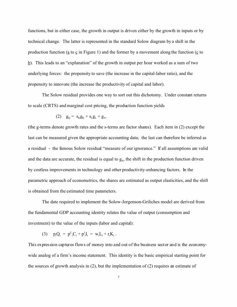
functions, but in either case, the growth in output is driven either by the growth in inputs or by

technical change. The latter is represented in the standard Solow diagram by a shift in the

production function (a to c in Figure 1) and the former by a movement along the function (c to

b). This leads to an “explanation” of the growth in output per hour worked as a sum of two

underlying forces: the propensity to save (the increase in the capital-labor ratio), and the

propensity to innovate (the increase the productivity of capital and labor).

The Solow residual provides one way to sort out this dichotomy. Under constant returns

to scale (CRTS) and marginal cost pricing, the production function yields

(2) gQ = sKgK + sLgL + gA.

(the g-terms denote growth rates and the s-terms are factor shares). Each item in (2) except the

last can be measured given the appropriate accounting data; the last can therefore be inferred as

a residual - the famous Solow residual “measure of our ignorance.” If all assumptions are valid

and the data are accurate, the residual is equal to gA, the shift in the production function driven

by costless improvements in technology and other productivity-enhancing factors. In the

parametric approach of econometrics, the shares are estimated as output elasticities, and the shift

is obtained from the estimated time parameters.

The date required to implement the Solow-Jorgenson-Griliches model are derived from

the fundamental GDP accounting identity relates the value of output (consumption and

investment) to the value of the inputs (labor and capital):

(3) ptQt = pCtCt + pI

tIt = wtLt + rtKt .

This expression captures flows of money into and out of the business sector and is the economy-

wide analog of a firm’s income statement. This identity is the basic empirical starting point for

the sources of growth analysis in (2), but the implementation of (2) requires an estimate of

8

output and inputs in constant rather than current prices. This can be done by separating the

consumption, investment, and labor income flows in (3) into price and quantity components

using published indices; the capital income flow, however, presents a problem. Neither the price

nor quantity components of rtKt are directly observed. (In terms of quantities, the current

measurement system provides a measure of It but not Kt.) Indirect methods must therefore be

employed to isolate the quantity component of capital in order to calculate its growth rate.

The basic two-step procedure used to solve this problem was developed by Jorgenson

and Griliches (1967). The estimate of It from the left-hand side of (3) can be used to impute a

capital stock using the perpetual inventory model:

(4) Kt+1 = It + (1-*)Kt.

Investment in each year is added to the preceding year’s stock, which is adjusted for retirement

and in-use lost of productivity (we assume a constant rate of deterioration/depreciation for

simplicity of exposition). An estimate of the initial stock of capital, K0, serves as the starting

point for the perpetual inventory method. This procedure must be implemented for every

category of investment good included as part of the aggregate of It. Note that this procedure has

the feature that whatever is included in I will be included in K.

Aggregate capital income rtKt must then be allocated to each type of capital good when

more than one type exists. Following Jorgenson and Griliches, this is accomplished using the

Hall-Jorgenson user cost for capital good j:

(5) ,

where it is the overall nominal rate of return to capital. Given a user cost for the jth type of

capital and the corresponding stock, a separate rjtKjt can be computed for each type of stock and

9

the result used to calculate a share-weight for use in constructing a capital aggregate and the

Solow residual. Such a procedure, however, will not separately identify the influences of

capacity, markup, and scale effects, and these factors may become embedded within the

estimated return to capital.

Despite the power of this approach, the theory behind it is not helpful in addressing the

problem of which input and output should be included in the analysis, because the production

function (1) only asserts that there is a stable relation between output and inputs. Indeed, the

production function is a structural equation embedded in a larger model, and by itself offers no

explanation of the evolution of labor, capital, and technical innovation. These variables are

treated as exogenous, without any rule for determining how the variables ought to be defined or

which belong in the analysis. Thus, this framework fails to provide guidance on a host of

questions about the “boundaries” of economic variables: Should output be measured gross or net

of depreciation? What “razor” should be used for determining which inputs are intermediate and

which should be capitalized? How should intangible inputs and outputs be treated? Should

capital-embodied technical change be ignored or explicitly included?

We will approach these boundary problems by embedding the production function in a

larger framework in which the variables of interest are endogenized. There are a number of

options in this regard: the Solow-Swan and Cass-Koopmans neoclassical growth models

endogenize capital formation, and the Lucas-Romer endogenous growth models endogenize

technology and capital (see also Barro and Sala-i-Martin 1995). In an empirical context, Rymes

(1971) and Hulten (1975,1979) examined some of the implications of the endogeneity of capital

for growth accounting using the conventional accounting model (2), and Mankiw, Romer, and

Weil suggest an alternative model based on the Solow-Swan model. In the following section of

3Of course, in a measurement world with chain weighting, real output does not equal the simple sum of C and I if the

relative price s of consum ption and in vestment are changing. H owever, to keep the ex position simp le, we will

assume that the re is a single outp ut that can be u sed either for c onsump tion or investm ent. We w ill relax this

assumption in our empirical work.

10

this paper, we continue this line of analysis but apply it to the problem of model specification

and the appropriate measurement of capital and technology variables.

B. Fisherian Optimal Growth

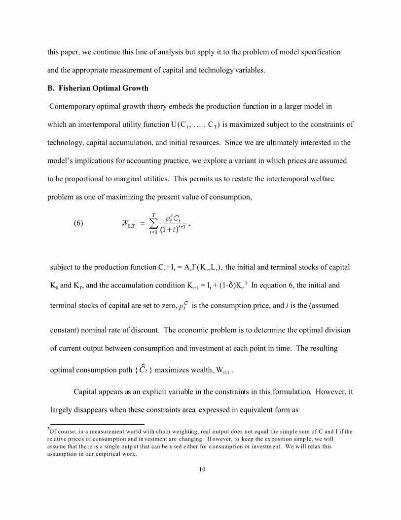
Contemporary optimal growth theory embeds the production function in a larger model in

which an intertemporal utility function U(C1, . . . , CT) is maximized subject to the constraints of

technology, capital accumulation, and initial resources. Since we are ultimately interested in the

model’s implications for accounting practice, we explore a variant in which prices are assumed

to be proportional to marginal utilities. This permits us to restate the intertemporal welfare

problem as one of maximizing the present value of consumption,

(6)

subject to the production function C t+I t = A tF(K t,L t), the initial and terminal stocks of capital

K0 and KT, and the accumulation condition Kt+1 = It + (1-*)Kt.3 In equation 6, the initial and

terminal stocks of capital are set to zero, is the consumption price, and i is the (assumed

constant) nominal rate of discount. The economic problem is to determine the optimal division

of current output between consumption and investment at each point in time. The resulting

optimal consumption path { } maximizes wealth, W0,T .

Capital appears as an explicit variable in the constraints in this formulation. However, it

largely disappears when these constraints area expressed in equivalent form as

11

(7) M({C1, ... , CT};{L1, ... , LT};{A1, ... , AT}; K0, KT) = 0 .

This is the intertemporal production possibility frontier, indicating all combinations of the

consumption vector {C1, ... , CT} that are possible given the vector of labor input, costless

technology levels, and the initial and terminal stocks of capital. Setting the initial and terminal

stocks of capital to zero eliminates the explicit presence of capital (and simplifies the exposition

of the intertemporal optimization problem).

The intuition behind this formulation is shown in Figure 2 for the case of two time

periods. The feasibility constraint M is represented by the curve AB, and the intertemporal

utility function U(C1, ... , CT) by the curves UU and U'U'. The optimal consumption plan is

represented by the point a, and this point defines the maximal wealth of the economy WW. The

optimal point is an explicit function of labor input and level of technology in each period.

Capital is implicit in the optimal solution, because A-C1 units of consumption are foregone in

period 1 and the resources freed-up by this abstinence are used to make capital goods, which are

then used up in production in period 2. Capital is in effect an intermediate intertemporal good .

The relative roles of capital formation and technical change can be explored using the

following thought experiment: What would have been the outcome had technology not

increased from A1 to A2, with labor held constant? The production possibility frontier in the

case of zero technical change is shown as the curve AB', and the optimal solution as b. The

effect of capital formation on the optimal consumption plan (in the absence of technical change)

is represented by the notional jump from A to b, and the effect of technical change (including

the effect of the induced capital accumulation) as the jump from b to a. The latter is the

"wealth effect" of technical change much discussed in recent years, but note that it arises only

from unexpected increases in the level of technology. Expected increases in technology are

12

already embedded in the long-run consumption plan of the optimizer (that is, C1 is invariant to

expected technical change).

Under certain circumstances, the optimal trajectory implied by the maximization of the

(6) subject to (7) converges to a balanced growth path (Cass (1965) and Koopmans (1965)).

For optimal consumption paths that do not necessarily lie on a balanced path, the results of

Weitzman (1976) are useful in augmenting the basic Fisherian accounting framework implied

by (6) and (7). We turn to this issue in the following section.

III. NET AND GROSS OUTPUT, WELFARE AND GROWTH

A. Net and Gross Output: Theory

In his seminal contribution, Solow (1957) defined output as net of depreciation, and calculated

his TFP residual accordingly. This approach was also taken by Denison, but Jorgenson and

Griliches (1967) advocated the use of gross output. Advocates of the net output argue that the

net concept provides a better indicator of the welfare gains from economic growth than does the

gross output concept, because gross output can be increased by using up capital and natural

resources. Advocates of gross output point to the fact that factories and businesses do not

produce units of output net of depreciation, and if the objective is to measure the growth in

productive efficiency, gross output is the right concept.

The intertemporal framework developed in the preceding section makes a useful

contribution in resolving this debate. Weitzman (1976) shows that the optimal solution to the

intertemporal optimization problem implies an “annual” measure of the increase in consumer

welfare: , where the “hats” imply optimal solutions to the problem (6) and (7).

13

This term – consumption plus the net change in capital – is really nothing more than the

Hicksian definition of income: the maximum amount of output that could be consumed each

year without reducing the original amount of capital (or “sustainable” consumption). It is also

the definition of Haig-Simons income: consumption plus change in net worth. A little algebra

also reveals that it is equivalent to gross product, as defined in (3), less economic depreciation

(Hulten 1992). Thus, the usual measures of income and net product fall out of the

intertemporal optimization problem and are indicators of the annual increase in consumer

welfare.

These results may seem to encourage the view that NDP should be used instead of GDP

in computing TFP-like residuals. However, this is not the case. The improvement in welfare

made possible by technical change is a matter of the “A” terms in the welfare constraint shown

in equation 7. The TFP residual computed using real gross output is the right measure of each

“A,” not the net-output TFP residual. What, then, is the right way to link welfare to

productivity? We will see in the following section that the correct welfare concept is a linear

function of the gross-output TFP residual.

14

B. The Dynamic-Welfare Residual

Equation 6 expressed the increase in wealth (welfare) from period 0 to period T as:

(8)

,

where and are the prices of consumption and capital goods, respectively, and is the

wage rate of labor. The first equality in equation 8 is, in effect, the intertemporal budget

constraint of the economy, the analogue of the static constraint (3). The second equality shows

that the accumulation of wealth can be expressed as the discounted sum of wage payments.

To go to the next step, Hulten (1992) totally differentiated equation 8 to yield an

expression parallel to the Solow residual that allocates the change in wealth to its sources. For

the period from period 0 to period T, this exercise yields the residual S0,T, defined as:

(9)

4There is a d ifference in the timin g conventio n used in this de compo sition relative to the conventio nal SOG analysis.

The conventional decomposition of output growth provides year-by-year figures that often are averaged together

across years to gauge average contributions of different sources of growth over time. In contrast, the S0,T residual

does not p rovide yea r-by-year figures, b ut rather pro vides a single b reakdow n for the full perio d from pe riod 0 to

15

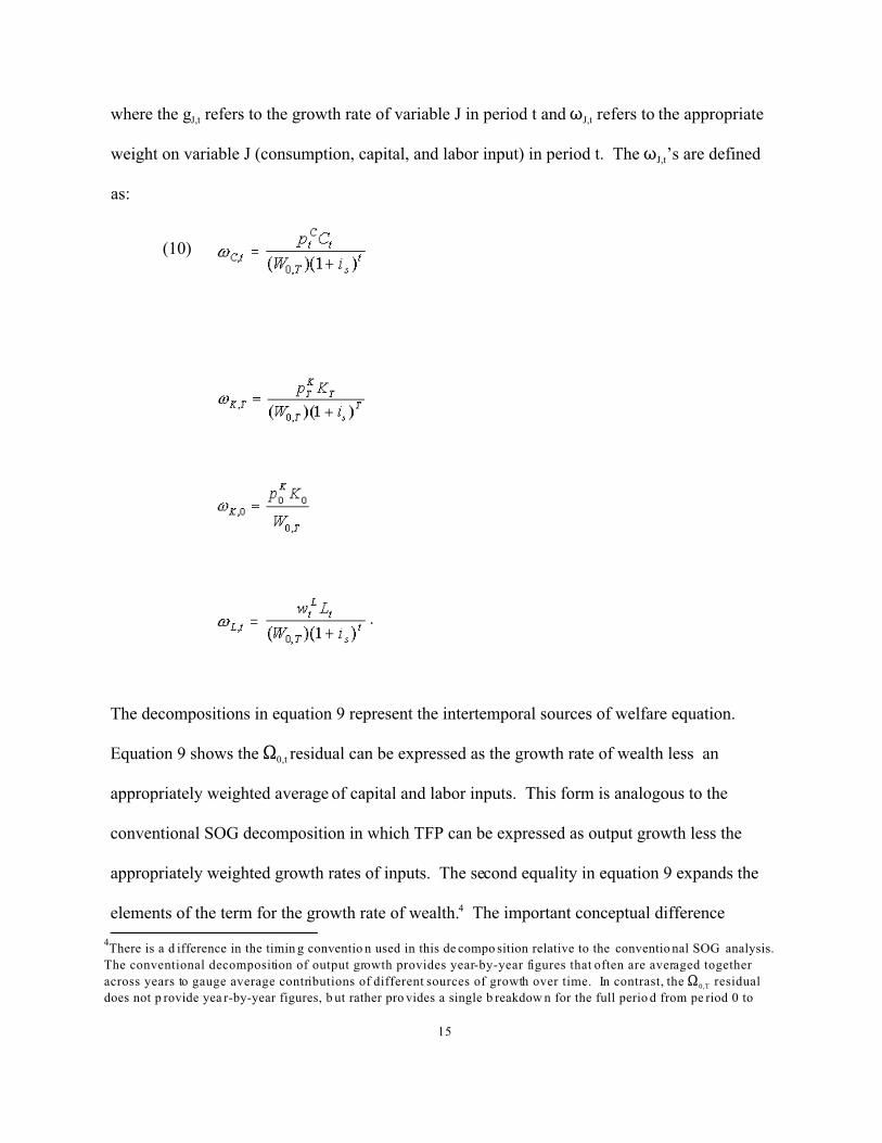
where the gJ,t refers to the growth rate of variable J in period t and TJ,t refers to the appropriate

weight on variable J (consumption, capital, and labor input) in period t. The TJ,t’s are defined

as:

(10)

.

The decompositions in equation 9 represent the intertemporal sources of welfare equation.

Equation 9 shows the S0,t residual can be expressed as the growth rate of wealth less an

appropriately weighted average of capital and labor inputs. This form is analogous to the

conventional SOG decomposition in which TFP can be expressed as output growth less the

appropriately weighted growth rates of inputs. The second equality in equation 9 expands the

elements of the term for the growth rate of wealth.4 The important conceptual difference

period T.

16

between the S0,T residual and the Solow TFP residual gA lies in the interpretation: the Solow

TFP residual measures the shift in the production function due to costless improvements in

productive efficiency (figure 1), while the S0,T residual measures the resulting shift in the

intertemporal consumption possibility frontier (figure 2). The S0,T residual is thus a measure of

the improvement in economic welfare over the time interval from period 0 to period T arising

from the annual shifts in technology, gA. For this reason, we will use the term “dynamic

welfare residual,” or DWR, when referring to S0,T.

This intuitive linkage is verified in Hulten (1979 and 1992), where it is shown that DWR

can be expressed as the weighted sum of the conventional TFP residuals:

(11) .

where Tt is:

(12)

Equation (12) indicates that the weight, , equals the ratio of current-dollar gross output in

period t discounted back to the base period and the denominator is the total amount of wealth

accumulated over the period as given by equation 8. Equation (11) shows that the conventional

TFP residual and the DWR are complements, not substitutes.

It is no accident that the weights in equation (12) sum to an amount greater than one.

This reflects the intermediate good nature of capital, which allows us to appropriate the Domar

weighting scheme developed to aggregate Solow TFP residuals across industries (Hulten

17

(1978)). In the interindustry case, the Domar weights are the ratio of nominal gross output in an

industry to the sum of nominal final demand across industries (GDP). These weights sum to an

amount greater than one to reflect the leverage that productivity change at the industry has on

aggregate output, because of the induced expansion in intermediate inputs. In the case of the

DWR, the weights sum to more than one to reflect the effect that productivity change has on

total consumption, because of the induced expansion in capital as an intertemporal intermediate

input.

This point can be elaborated in terms of NDP, which we have seen is equal to Haigs-

Simons-Hicks-Weitzman income: . Note that the intertemporal budget

constraint (8) can be re-expressed as the equality of the discounted present value of

on the one hand, and the present value of labor income on the other.

DWR can be shown to be equal to the share-weighted average of the NDP-based

residuals, where the weights are analogous to equation 12, but are based on NDP and sum to

one. The individual NDP-based residuals are therefore not to be interpreted as the correct

welfare-based measure of productivity. However, it is true that if the NDP residuals are

constant over time, they are equal to DWR.

Some further linkages between DWR and other growth-related measures are worth

noting. We noted in section II above that the optimal consumption path may converge to a

balanced-growth path under certain conditions. One condition is that productivity grow at a

constant Harrodian rate, gH.. The Harrodian rate is defined as the shift in the production

function (1) measured with respect to a constant capital-output ratio (along the line a to b in

5 These steady-state relationships are more complicated in a multi-sector model. For example, see Oliner and

Sichel (2002).

18

figure 1), whereas the Hicksian rate, which underlies the Solow residual, is measured along a

constant capital-labor ratio (along the line a to c in figure 1).

Thus, the Harrod rate, gH, which includes induced capital accumulation, is equal to the

Hicksian-Solow-Residual rate, gA, divided by labor’s share of income, as in gH = gA / sL. With a

little algebra (see Hulten (1992)), it can be shown that the DWR equals the constant Harrodian

rate on a balanced-growth path. The reason that the contribution of TFP growth is “blown up”

in steady state is that TFP growth induces capital accumulation and, ultimately, the pace of

capital accumulation in steady state depends on TFP growth.5 Thus, on a balanced-growth path

in steady state, DWR also equals the long-run contribution of TFP to output growth.

These linkages between DWR, the Harrodian rate of technical change, and the steady-

state contribution of TFP to output growth in a simple one-sector model provide some comfort

that the DWR is simply a generalization of a familiar concept and not some exotic way of

looking at growth accounting. Moreover, the link between DWR and Harrodian technical

change provides an interesting interpretation of Harrodian technical change. Namely,

Harrodian technical change is more than just the shift in the production function along a

constant capital-output ratio; under certain conditions it is a valid measure of the increase in

consumer welfare made possible by the shift.

C. Net and Gross Output: Empirical Analysis

In this section, we put some rough numbers on DWR and other TFP-type residuals using

conventional published data. These numbers will help to make the concept of DWR concrete

6For example, see Oliner and Sichel (2000), Oliner and Sichel (2002), Jorgenson and Stiroh (2000), Jorgenson, Ho,

and Stiroh (2002), and Gordon (200 2).7BEA publishes real net domestic product for the nonfarm business sector less housing back to only 1987. For

growth rates fro m 1987 and back , we used the g rowth rate in re al net dom estic produ ct for the total eco nomy.

19

and to cement ideas about how DWR relates to other TFP-type residuals. This illustration is

most effective using a database that is widely familiar to analysts.

Table 2a shows numbers for the key concepts. Before discussing DWR, it is useful to

review results for conventional residuals based on gross and net output. The first column shows

the conventional TFP numbers based on real GDP in the nonfarm business sector (less housing)

for selected periods. (Note that the gross output TFP numbers for the nonfarm business sector

in table 2a differ from those in table 1 only because of differences in the time periods shown.)

Between 1950 and 1973 – the so-called golden era of productivity growth – TFP rose an

average of about 1.7 percent per year (line 1). Following the productivity slowdown in 1973,

TFP growth from 1973 to 1995 dropped back to just 0.4 percent per year. Then, from 1995-

2000, TFP growth picked up to about 1.2 percent per year, a substantial improvement over its

lackluster pace during the prior twenty-some years.

This pattern of TFP – and particularly its role in the productivity resurgence of the late

1990s – has received much attention from economists.6 As discussed above, these conventional

TFP numbers provide useful information about shifts in the production constraint. However,

other measures also provide important insights into the nature of economic activity.

We show the residuals based on net domestic product in the nonfarm business sector in

column 2 because they have received attention in the past.7 Interestingly, the “net” TFP figures

remarkably similar to those based on gross output. Thus, even if one were to disregard the

arguments laid out above and use residuals based on net domestic product as an indicator of

8Figures are not reported for short periods because, conceptually, these calculations pertain to forward-looking

behavior where agents are thinking about long-term wealth (welfare) maximization; very short horizons are not

really consistent w ith this long-term p erspective. A lso, calculation s over shor t periods o f time tended to be unstab le

in the sense that ex tending the time horizon b y one year o ften changed the numerica l results conside rably.

20

welfare, the numbers in table 2a suggest that the story delivered by the NDP ( )

residuals would be essentially the same as that by the GDP residuals ( ).

Column 3 of table 2a shows average annual growth rates of DWR (S); these residuals

rose nearly 2.5 percent per year from 1950 to 1973, but then slowed dramatically in the period

from 1973 to 2000 to a pace of just about 0.8 percent. Although the period from 1995-2000 is

too short to obtain sensible estimates of DWR, a comparison of lines 2 and 3 indicate that

growth rates S0,T and wealth are noticeably higher when the period extends to 2000 than when

it ends in 1995.8 More generally, note that the growth rate of DWR is larger than growth rates

of the conventional residuals shown in columns 1 and 2. This occurs because DWR takes

account of the capital accumulation induced by technical change, whereas the conventional

residuals only capture the proximate sources of growth and do not take account of capital

accumulation induced by technical change.

Column 4 of the table shows our estimate of Harrod TFP, which is defined as

conventional TFP based on gross output (column 1) divided by the average income share of

labor over the period shown. What is striking about these numbers is how similar they are to

the growth rates of DWR in column 3. For example, Harrod TFP increased at an average

annual rate of about 2.4 percent from 1950-1973, just about the same rate of rise as DWR over

that period. Similarly, during 1973-2000, the Harrod TFP rose about 0.8 percent per year, the

same rate as the dynamic residual. More generally, the analysis here highlights the degree to

9The smaller share of output growth explained by TFP growth in the 1995-2000 period relative to the 1950-1973

period reflects the substantial pickup in capital deepening that also occurred during 1995-2000.

21

which conventional TFP based on gross output, DWR, and Harrod TFP are complements that

illuminate different aspects of growth and welfare.

The numbers in table 2b highlight another way in which conventional TFP and DWR

provide information about different economic concepts. This table shows the fraction of real

GDP growth in the nonfarm business sector explained by the conventional TFP residual and the

fraction of increases in wealth explained by DWR. This key pieces of this relationship for

conventional TFP are shown in the first three columns of the table. The first column repeats the

numbers from table 2a for , the second column shows the growth rate of real output

in the nonfarm business sector less housing, and the third column displays the fraction of output

growth explained by TFP (the ratio of column 1 to column 2). As shown in column 3, TFP

explained more than 40 percent of output growth from 1950-73. This share dropped back

sharply after 1973, but recovered somewhat after 1995. Despite the recovery, from 1995-2000,

TFP growth accounted for only about 26 percent of output growth over this period, a smaller

fraction than during the period from 1950-1973.9

Columns 4 to 6 show a parallel set of calculations for DWR. Column 4 repeats the

numbers for DWR from table 2a, column 5 shows the average annual increment to wealth (as

defined in equation 8), expressed as a growth rate. Column 6 displays the fraction of wealth

gains explained by the DWR; that is, the ratio of column 4 to column 5. From 1950-73, DWR

accounted for more than 60 percent of the robust gains in wealth; that is, technical change

accounted for 60 percent of the increase in wealth 1950-73. In contrast, from 1973-2000 (line

10Column 6 could also be interpreted as showing the steady-state contribution of TFP growth to output growth in a

simple one -sector mod el.

22

2), the rate of increase in wealth fell back somewhat, but the fraction of that wealth gain

explained by technical change dropped substantially to just 24 percent.

A comparison of columns 3 and 6 yield an interesting observation. Namely, the fraction

of gains in wealth explained by DWR (column 6) are larger than the fraction of output growth

explained by TFP in the conventional analysis (column 3). This occurs because the extended

framework allows for the full effects of changes in TFP over time; that is, increases in TFP

induce future capital investment. The conventional SOG framework does not take account of

the effect of that induced capital formation on output growth, while the extended framework

does account for the effect of that induced capital formation on future wealth gains. Put another

way, column 3 summarizes the role of conventional of TFP on output growth, while column 6

shows how this output growth contributes to welfare after taking account of induced capital

accumulation in subsequent periods.10

IV. THE SCALE OF BUSINESS INVESTMENT

Although the precise determinants of the pickup in U.S. productivity in the late 1990s shown in

tables 1 and 2a remain a subject of debate, most observers ascribe an important role to one or

more of these factors: the enhancement of business performance made possible by computers

and related technology, the increased availability of new products and new production

processes, and improvements in “firm dynamics” made possible by new workplace practices.

However, a significant chunk of the spending related to these activities is for intangibles and is

23

not accounted for in the standard SOG analysis. In this section, we begin to confront the

boundary issues related to intangibles by applying the framework discussed in Section II.

A. Implications of the Intertemporal Framework for Measurement.

The model and framework presented in section II has several important implications for current

measurement practices. First, Figure 2 makes clear that any use of resources that reduces

current consumption in order to increase it in the future (for example, the movement along AB

from the point A on the horizontal axis to the optimal point a) qualifies as an investment. Thus,

if resources are devoted to R&D to generate innovations that increase future consumption, an

investment has occurred. (The same is true of students’ deferral of entry into the labor force in

order to pursue a higher education.)

Put differently, Figure 2 argues for symmetric treatment of all types of capital. As a

result, there is no theoretical basis for treating investments in knowledge and human capital any

differently than investments in plant and equipment in national economic accounting systems.

One way to treat all capital symmetrically would be to add knowledge and human capital to the

“I” in “C+I+G.” An alternative approach, indeed, the full logic of the section II, argues for

treating capital as an intertemporal intermediate input. The appropriate accounts are then

intertemporal and based on a functional form for (1) that links labor input and technology

directly to the attainable consumption path; intertemporal accounts drop capital (except for

noting the initial and terminal period values).

Real world accounting systems are not intertemporal, however, and pursuing the full

logic of Figure 2 does not imply dropping conventional procedures. Real world systems need to

include investment because they report data according to the GDP identity (3) and, implicitly, a

24

recursive scheme for capital that is based on a fixed “length” for the accounting period. The

periodicity is the choice of the accountant.

An aspect of the specific choice of a length for the accounting period, usually one year,

bears mention. Although it is an arbitrary figure, the choice of a length for the accounting

period determines what is a “fixed” asset and what is an intermediate input (or consumption):

If a system of accounts selects a daily periodicity, inventories of pencils and paper are fixed

capital; if the accounting period is five years, much high-tech equipment and software are

intermediate inputs; and if the period is 100 years, almost all equipment purchases would need

to be expressed as intermediates. The intertemporal model thus implies that the scale of

business fixed investment and GDP is somewhat arbitrary, whereas the underlying economic

welfare, measured by (8), is invariant to the choice of the accounting period.

Note that because what becomes fixed investment is arbitrary, what becomes inventory

investment is also arbritary in this model. Any input that is not used for current consumption

and is intended to increase future consumption is “capital” in the sense of section II, even if it is

not classified as fixed capital. Such an input would simply be an inventory carried over for

future use. Indeed, in the framework of Section II, all capital is an inventory of intermediate

goods.

To summarize, the intertemporal framework presented in section II suggests that

business expenditures designed to raise productivity or increase the range of production

possibilities in the future is investment, while those that are inputs to production processes and

used up within the accounting period are intermediate consumption. Moreover, from a national

accounts perspective, the framework offers a clear guideline for the categorization of many

types of business expenditures as either fixed investment or intermediate inputs: Is the

25

replacement cycle of the input less than/greater than the accounting period selected? And, the

framework reminds us that, when changes in produced intermediates can be identified and

valued, they must be included in inventory investment and the corresponding asset recorded on

the national balance sheet.

B. Basic Types of Investment and Capital

Following Lev (2001), we interpret and use the terms “knowledge capital,” “intangibles,” and

“intellectual property” interchangeably, and note, as he has, the tendency of economists to use

knowledge capital, while intangibles is used in the accounting literature and intellectual capital

and/or intellectual property in the management and legal literature. Moreover, economists have

tended to view human capital as a significant component of knowledge capital. The scope of

knowledge capital is thus quite broad; the problems of classification and measurement vary

from type to type; and the size of the bias resulting from the exclusion of each type must be

considered separately.

Human capital, whether produced by the household sector (through their deferral of

entry into the labor market) or by the education sector (through spending on formal education)

is not treated as an asset on the national balance sheet. Measuring the output of the educational

sector and the impact of household sector investments in human capital poses an immense

challenge. Many important aspects of that challenge have been addressed in an impressive

body of work by Dale Jorgenson, Barbara Fraumeni, and others (Jorgenson and Fraumeni

1989a, 1989b, 1992; Eisner 1989; Ironmonger 1996, 1997; Landefeld and Howell 1997; and

Jorgenson, Ho, and Stiroh 2002), however. A major result is that the household account

expanded to include their human capital investment is very large: The available estimates run

from 40 to 300 percent of the existing GDP (Fraumeni 2000).

11 In 1999, however, BEA substantially broadened its core business investment measure by adding computer

software, a major type of intangible asset. T hus, some business intangibles are represented in the U.S. national

accounts, contrary to what some commentators suggest. BEA estimates that business spending on software was

more than $160 billion annually in the late 1990s, a noticeable amount, but not large enough to satisfy these and

other critics of the current NIPA measures.

26

At this point, we turn to non-human knowledge capital produced by the private business

sector, and we will not explore human capital in the household sector further. How large might

such spending be? Some observers have suggested that official GDP and business investment

measures are vastly understated because they are limited to capturing spending for tangible,

physical assets, rather than expenditures for legally recognized intangible assets, such as patents

and copyrights. Nakamura (2001) places the undervaluation of business investment in the late

1990s in the neighborhood of $1 trillion annually, roughly 10 percent of the existing GDP.

Brynjolfsson and Yang (1999) argue that, for each dollar spent on computer and computer-

related hardware, nine more are spent on related intangibles, implying that at least $750 billion,

or more than 8 percent of existing GDP, is being missed by business spending on IT-related

intangibles.11

These figures suggest that a move to the accounting logic of the intertemporal model,

which suggests that business intangibles (and human capital) should be recognized in national

accounting systems (or satellite accounts), could result in a significant changes in measures of

economic activity. The remainder of this section presents our best attempts to put some

numbers on intangibles spending by the business sector.

C. The Accounting Period of Capital: An Examination of Current Practice.

The 1993 System of National Accounts (SNA) acknowledges that the period of accounting is a

choice of national accountants, but advises them to choose a period of at least one year so that

12 The information in this paragraph was obtained in conversation with Brent Moulton, Associate Director for

National Accou nts, Bureau of Econ omic Analysis.

27

seasonal effects are avoided. Longer periods “may not adequately portray changes in the

economy ... [while] ... periods that are too short have the disadvantage that statistical data are

influenced by incidental factors.”

With regard to the U.S. NIPAs, different sectors apply different accounting periods for

capital, and there is no single recent statement that represents the choices in the system.12 For

business and government, according to a more than 25-year-old study, equipment is defined as

durable goods having an average service life of more than one year; for households, equipment

(consumer durables) is defined as durable goods having an average service life at least three

years (Young and Musgrave 1976). In practice, the available source data introduces additional

twists in BEA practices: For example, the Census of Governments uses five years as a cut off

to determine whether a purchase is equipment. But, for the business sector, where the flows are

built using data by asset type according to the commodity-flow method (see Grimm, Moulton,

and Wasshausen 2002), the NIPAs currently do not recognize any assets having a service life of

less than three years.

If the NIPAs maintain current practice and essentially define fixed assets as inputs with

a useful service life of at least three years, the recognition of intangibles, many of which are

inherently elusive and not long-lasting – such as certain types of advertising – could have a

relatively small effect on measured business fixed investment. On the other hand, if the

accounting period selected for the NIPAs is really just one year, and if the BEA were to

recognize business intangibles, many types of business expenditures may need to be counted as

fixed assets, and measured business fixed investment could be scaled upward by a noticeable

amount.

28

D. Identifying and Measuring Spending on Business Intangibles.

The literature on intangible capital approaches the problem of classification from different

starting points (eg. Lev 2001, OECD Secretariat 1998). Despite the different starting points,

however, the attempts generate similar classifications and similar lists of items that represent

private business spending on intangibles.

Table 3 summarizes the items that have been most commonly cited and groups them

into three broad categories, similar to groupings used by Lev and others (eg., Khan 2001). The

grouping suggests that the knowledge capital of a firm consists of the following components:

computerized information, technology and innovative property, and economic competencies.

The table also indicates whether the current NIPAs or the 1993 Systems of National Accounts

(SNA) categorizes each type of spending as intermediate consumption or fixed investment and

provides brief comments on the availability of data for each item. Finally, table 3 presents an

estimated size range for each broad group; in some instances, these are based on highly

preliminary and/or rudimentary estimates for the individual items shown.

Computerized information. This component reflects knowledge embedded in computer

programs, and we estimate that investment in this category of knowledge capital ranged from

$145 billion to $165 billion annually in the late 1990s.

When computer software was recognized in the NIPAs in 1999, not only were purchases

of prepackaged and custom software newly counted as investment, the estimated costs of

software created by firms for their own use also were included. The own-account estimates

were developed from detailed occupational data on employment and wages in private industry,

in conjunction with an estimate (50 percent) of the average time spent by individuals in the

relevant occupations on “software development” (Parker and Grimm 1999). This method of

13 Much o f the produ ction of com puterized database s probab ly is done by firm s for their own u se. Thus, so me, if

not all, of computerized database production may already be included in NIPA own-account computer software, and,

as a result, a separate own-account estimate for computerized database is not included.

The figure cited in the text, less than $2 billion, reflects the 1998-2000 average annual revenue of the new

NAICS industry, database and directory publishers (excluding advertising sales, contract printing, and other) as

reported in the 2000 Services Annual Survey (SAS), issued by the Census Bureau.14 Indeed, the software that is bundled with the sale of a computer is already included in figures on computer

purchase s.

The figure cited in the text reflects the1998-2000 average annual revenue for the system software sub-

category of the NAICS industry, software publishing, as reported in the 2000 SAS. Only a very small deduction

was made for the software bundled with equipment sales, consistent with the assumptions built into the current

NIPA estimates.

29

estimating investment, though imprecise, is consistent with the framework of Figure 2: Some

uses of time (development) are investment, others uses (maintenance and routine repair) are

consumption.

The upper end of the range for spending in this category reflects the NIPA computer

software estimates for 1998 to 2000 (which averaged about $160 billion) plus a small figure

(less than $2 billion) for computerized databases, an item not capitalized in the NIPAs.13 The

lower end of the range reflects the subtraction of the value of systems software currently

included in the NIPA figures (about $15 billion). Even though the intertemporal framework

does not address the boundary between tangible and intangible investments, the lower bound

accommodates a position held by some that the software that controls the basic function of the

computer (systems software) should be classified as a tangible investment (e.g., Clement, et. al,

1998, Vosselman 1998).14

The bounds in the table also reflect the preliminary nature of the current NIPA estimates

for computer software. Although BEA made innovative use of the limited data and research

available when the estimates were introduced in 1999, the BEA’s commodity-flow method

requires a current benchmark Input-Output (I-O) table to reliably estimate GDP components

from source data on industry production and trade. Moreover, a great deal more statistical

15 For purch ased softwa re, the refineme nts include the in clusion of imp roved estim ates of the softwa re bundled with

other equipment and more accurate data on exports and imports; for own-account software, improved employment

and wage data will be used to estimate production. These changes are expected to reduce business spending on

software (see Moylan 2001).

Beginning in 2003 the Census Bureau hopes to have developed a new quarterly indicator survey covering

the output o f the software ind ustry (pre-pac kaged an d custom) ; the availability of this ne w, more co mprehen sive data

will substantially enhance the accuracy of the quarterly NIP A measures.16 This point is emphasized in the OECD work on intangibles (e.g., Vosselman 1998, Khan 2001).

The BEA m akes an adjustment to exclude software R&D from own-account software. Currently, the

adjustment is largely judgmental, but it will be refined with the introduction of the 1997 benchmark I-O table in the

2003 b enchmark NIPA revision. (Co nversation w ith Carol M oylan.)

30

information on computer software is now available, and the current NIPA estimates will be

substantially refined and updated for the 2003 benchmark revision.15

BEA’s experience with the capitalization of computer software illustrates several of the

challenges intangible capital poses for national accountants. First, when production is carried

out by firms for their own use and must be estimated, information on employee uses of time is

required – here, software maintenance/repair versus software development. A paucity of this

type of information, both at a point in time and over time, is not limited to employees that

create and develop computer software. Second, conceptual problems frequently arise when

own-account production is estimated; here, because software is a tool in research and

development, there is a conceptual overlap between the figures for own-account software and

the available data on R&D expenditures.16 Third, the dynamism of industries producing and

investing in intangible capital may pose difficulties when standard estimating methodologies

are applied to basic survey data and I-O information that are out-of-date and/or incomplete.

Technology and innovative property. This is the “R&D” component of business

knowledge capital. It reflects the scientific knowledge embedded in patents, licenses, and

general know-how (not patented) and the innovative and artistic content in commercial

copyrights, licenses, and designs. Thus, both scientific and nonscientific types of product

development costs comprise business expenditures on “R&D.”

17 In contrast, as ind icated in the tab le, the SNA recomm ends treating R &D ex penditures as intermed iate

consumption rather than a fixed asset. Even though the aim of most R&D is new patents, new inventions, and new

processes, the SNA explicitly states that research and development expenditures “do not lead to the acquisition of

assets that can b e easily identified, q uantified and valued for b alance shee t purpose s,” and that be cause it is difficult

to meet these requirements, “the outputs produced by research and development ... are treated as consumption even

though some of them may bring future benefits.” 18 The NSF data also reveal the industrial composition of R&D. Most R&D is conducted in manufacturing and,

within manufacturing, mainly by makers of pharmaceuticals, computers, semiconductors, and communications

equipment. Nonetheless, the nonmanufacturing segment of total R&D has been growing rapidly in recent years, and

some have interpreted this development as suggesting that a broad trend toward R&D in services industries is under

way. The finding, however, reflects the growth of R&D in one nonmanufacturing industry, software publishing, as

well as the growth in biomedical labs and “science parks” serving manufacturers. In short, the industrial

composition of R&D reflects its definition.19 Note that, in contrast to R&D expenditures, the SNA states, “whether successful or not, .... [mineral exploration

is] ... needed to acquire new reserves and ... [the costs] ... are, therefore, all classified as gross fixed capital

formation.”

The figure cited in the text is the NIPA figure for mining exploration plus an estimate of the output of the

industry, geophysical surveying and mapping services, for which quinquennial data are available from the Census of

Mineral Industries.

31

According to most economic models and several decades of economic research

conducted by Zvi Griliches, Edwin Mansfield, and many others, R&D is unequivocally a

business investment.17 The R&D data that have been the subject of most of the research in the

United Sates, and the data that have been collected since the early 1950s for the National

Science Foundation, are “science and engineering” R&D. These data are defined to include

expenditures ... “on the design and development of new products and processes, and the

enhancement of existing products and processes,” but to only cover activities carried on by

persons trained, either formally or by experience, in the physical sciences, the biological

sciences, and engineering and computer science. As a result, measured private R&D is

conducted mainly by manufacturers and software publishers, and it was relatively high at about

$185 annually in the late 1990s.18 Adding in an estimate of mining R&D (about $15 billion),19

yields the lower bound shown in the table for the size of this broad category; that is, about $200

billion annually in 1998-2000.

20 Note that the SNA advises to treat these costs as investment, presumably because the spending leads to an

“identifiable” asset, such as a copyright or a broadcasting right, that can be recorded on a balance sheet. In the SNA,

the produ ced fixed a sset is called an “a rtistic or entertainm ent original.”

32

The upper bound of the technology and innovative property category reflects the

addition of a rudimentary estimate ($100 billion) of business resources devoted to technology

and innovation in other industries; see Nakamura 2001 for a discussion of the derivation of this

estimate. Information sector industries (book publishers, motion picture producers, and

broadcasters) and financial services industries routinely research, develop and introduce new

products, but we have no data on the resources they devote to these activities, that is, we know

very little about their R&D. Moreover, our knowledge of the production processes and new

product introduction patterns in these and other services industries is very limited.

With regard to nonscientific R&D, therefore, much needs to be learned. We need

broader industry coverage of the spending devoted to innovative activity. We also need to

know more about the development and process lags for each industry’s new products and the

productive lifetime of the innovative property created by the spending. For instance, is the

average economic lifetime of an original sound recording greater or less than three (or even 1)

years.20 Richard Caves (2000) points out that much of the spending on new products in the

entertainment industry pays off very quickly, while other costs are “paid for” by advertising and

still others (such as the cost of developing a new televison series and a new copyright film) are

investments that generate, on average, long-lasting revenue streams.

Economic competencies. This component of knowledge capital represents the value of

brand names and other firm-specific human and structural resources; sometimes the latter two

components are called “organizational” capital (Lev 2001), and sometimes the first is

designated as a separate component, “marketing.” Table 3 groups them together as business

21 (Authors note: This estimate is subject to refinement.) This estimate was derived using the information from a

special emp loyer survey co nducted b y the BLS in 1994 a nd from sim ilar surveys con ducted sinc e 1996 by a private

research firm (cite). <more detail to come>

33

expenditures designed to raise productivity and profits, other than the software and R&D

expenses classified elsewhere.

Even though the line of causality from a specific workplace practice, to organizational

change, to profitability in the marketplace is not entirely clear, most observers suggest that

investments in economic competency can be approximated by business spending for employee

training programs, organizational innovation and change (management time and management

consultant fees), market and consumer research, and advertising. As shown on the table, a raw

tally of estimates for these items suggests that spending on this component could have been

very large in the late 1990s, nearly $700 billion annually, or, considerably smaller but still large

at $200 billion per year. The wide range reflects data quality issues and classification

questions.

According to our framework and the results of research that has studied employer-

provided worker training at the firm-level (eg., see Black and Lynch 2000, Bassi, Harrison,

Ludwig, and McMurrer 2001), expenditures on workforce training and development, the first

item listed under this broad category, are an investment. We estimate that private businesses

spent between $15 and $65 billion on workforce training the late 1990s, a not large, but still

noticeable item.21 By contrast, we estimate that spending on organizational development and

change was a relatively large sum, maybe $300 billion (see below), and that outlays for brand

equity maintenance and development (represented by purchases of advertising services and the

22 The advertising data are fro m Bob C oen’s Insider’s Report , issued by Universal McCann at

http://www.mccann.com/insight/bobcoen.html. The data for the revenues market and consumer research industry

are from the 2000 SAS. Advertising expenditures were $215 billion per year from 1998 to 2000, and the market

research industry revenues were nearly $15 billion per year for the same period. The total cited in the text, $240

billion, ignore s expenses o n own-acco unt.

34

revenues of the industry, market and consumer research services), about $240 billion annually

from 1998 to 2000, did not all represent fixed investment.22

Investments in organizational change and development have both own-account and

purchased components, but not all outlays and resources devoted to managing and running an

organization are investment. Management consulting services revenues rose from $38.5 billion

in 1994, to more than $80 billion annually during 1998-2000. Because marketed purchases do

not include an own-account component and because a trend toward outsourcing may have

occurred, these figures understate the level of resources devoted to organizational development

and change but likely overstate its rate of growth. The own-account portion, executive time

spent in support of investment decisions, is viewed as proportional to the cost and number of

persons employed in executive occupations. In short, executive time is viewed as a proxy for

organizational change and development, as argued by Nakamura, Lev, and others.

The share of employment in executive occupations in total employment was less than 9

percent from 1950 to 1970, but it rose to more than 13 percent of total employment in 1994 and

to more than 15 percent by 2000, implying relatively rapid rates of change in the 1990s

(Nakamura 2001). And, given that executive median pay exceeds the median pay for other

employees, the fraction of total private payroll spent on executives and managers is

(conservatively) estimated to have been substantially larger, almost 22 percent in 2000

(Nakamura 2001).

23 Consulting expenses and the estimated value of executive time conceptually overlap by a small amount (the value

of executive time in the management consulting industry). Whatever that amount may be, however, it is dwarfed by

the use of an ar bitrary fraction fo r the amoun t of executive tim e devoted to organiza tional change and deve lopment.

In addition, some portion of management time arguably overlaps with nonscientific R&D (“organizational

R&D”), so that, for some industries, the line between industry-specific process innovation and organizational change

more gen erally may not b e drawn ea sily24 (Authors no te: This estima te is preliminary in th at compa ny formation expenses h ave not be en included .)

35

Applying the executive and manager payroll share to total private business sector

compensation, managerial and executive costs were nearly $1 trillion per year in the late 1990s

(1998 to 2000). If just one-fourth of management time is spent on organizational innovation,

then, businesses devoted another $250 billion per year to improve the effectiveness of their

organizations during this period.23 This figure is extraordinarily sensitive, of course, to the

admitted arbitrary choice of one-fourth as the fraction of time managers spend on investing in

organizational development and change; as a result, the lower bound on the table incorporates a

one-tenth fraction ($100 billion) and the upper more than one-third ($340 billion). Adding in

the annual expense for management consulting, our estimate thus centers on $300 billion per

year, with the lower bound at $180 billion and the upper at $420 billion.24

As indicated above, the marketing subcomponent is represented by purchases of

advertising services and the revenues of the industry, market and consumer research services.

The marketing literature has addressed the measurement of brand equity and the role of

advertising in creating brand equity at the firm level; it has also evaluated the effectiveness

(lifetime) of ad campaigns in specific media using statistical techniques and customer surveys.

This body of work needs to be rigorously evaluated for its economic measurement implications,

and more refined data and information may still be needed to determine the fraction of

advertising outlays and market research services that represents new information and brand-

building (investment), rather than maintenance expenditures (intermediate consumption).

36

Lacking this evaluation and such data, the range on table 3 incorporates an arbitrary lower

bound ($25 billion) for the advertising and market research that accompanies new product

introductions and an equally arbitrary upper bound ($215) that assumes that not all advertising

can constitute fixed investment.

D. Summing up the Measures on Business Spending on Intangibles

Business spending on intangibles may have exceeded $1 trillion annually in the late 1990s (the

sum of the upper bounds on the estimates in table 3). Moreover, we estimate that the full

recognition of business intangibles in the NIPAs would imply at least $420 billion in additional

business fixed investment spending during that period (the sum of the lower bounds on the

R&D and economic competencies components). Because remarkably little is known about

innovative activity outside of the industries that employ scientists and engineers and because

quantifying the precise investments that enable businesses to acquire increases in economic

competency is difficult, the tentative nature of the estimates presented in table 3 cannot be

underscored too emphatically. Nonetheless, one cannot escape the conclusion that spending on

unrecognized business intangibles was a substantial fraction of the existing GDP in the late

1990s.

We cannot readily assess the impact of our estimate of business spending on intangibles

on business sector net worth without improved information on the replacement cycle/service

lives of intangible assets. Thus, it is somewhat difficult to compare the implications of our

estimates for valuing the capital stock including intangibles to Bob Hall’s (2000) estimate that

the additional q-adjusted market value of intangibles amounted to about $4 trillion in the late

1990s. Of course, there is a rate of depreciation for knowledge capital that could reconcile our

upper- or lower-bound estimates with Hall’s, but sufficiently little is known about depreciation

37

rates for us to be very definitive at this point. But, bear with us: for example, if the stock of

knowledge depreciated at a rate of 18 percent per year, then very roughly speaking it would take

additional fixed investment spending of more than $700 billion annually to add $4 trillion to

business net worth in a simple steady state. This amount of spending is consistent with the

midpoint of the ranges of the R&D and economic competencies categories shown in table 3.

Even though this simple calculation is of interest, we do not have the information needed to

fully analyze how the productivity and welfare measures shown in tables 1 and 2a would

change if the boundaries of our current economic measures were expanded.

V. CONCLUSION

The remarkable performance of the U.S. economy in the second half of the 1990s has refocused

attention on identifying the underlying sources of economic growth. In the introduction of this

paper, we discussed some of the different strands of literature that have, in different ways,

started to stir the pot of growth and productivity analysis and measurement.

We too share the general sense that the conventional modeling framework and currently

available data are not telling us all that we need to know to understand economic growth. This

paper has attempted to take some first steps toward a broader framework for the economic

measurement of capital. This is a very difficult task, and we regard this paper as an effort put

some issues on the table for further thought rather than as a set of answers to some extremely

difficult questions.

On the theory side, described a growth framework that adds an explicitly intertemporal

dimension to the standard Solow growth-accounting framework. One important way in which

the extended framework is useful is by providing guidance on the “boundary” question of what

38

should be included as investment and therefore what measure of capital should be entered into

the production function. The conventional framework provides no guidance on this point, while

the extended framework yields the razor necessary to define investment: In particular, any use

of resources that reduces current consumption in order to increase consumption in the future

qualifies as an investment. Thus, a host of intangible investments – including R&D, copyrights,

computerized databases, development of improved organizational structures, brand equity, etc.

– should, in principle, be counted as investment. We also work through other implications of

this extended framework for measuring growth, technology, and welfare.

To show the power of this framework and how it relates to conventional growth

analysis, we presented estimates for key concepts of the extended framework – including a

dynamic welfare residual (DWR) – along with conventional gross output and net output TFP

residuals. These estimates are based on conventional published data in order to highlight the

linkages to earlier work using a traditional SOG approach. We argued that DWR is the

appropriate measure for gauging the contribution of technical change to the growth in wealth

(welfare). And, we show that growth rates of DWR are quite different from those of TFP

residuals based on net domestic product, a measure that some analysts have suggested –

incorrectly in our view – is the most appropriate for relating technical change to welfare. DWR

also grows more rapidly than conventional TFP (based on either gross or net product) because,

in the intertemporal framework, DWR accounts for the capital accumulation that is induced by

technical change. Finally, we demostrated that DWR is closely related to measures of technical

change from the conventional framework. Thus, argued that DWR is not a new, exotic way to

think about growth, but rather a measure that complements the traditional SOG framework.

39

As we indicated, this empirical implementation of the extended intertemporal

framework does not go beyond conventional measures. To do so requires confronting a host of

practical issues given severe data limitations. To take a small step in terms of practice, we have

pulled together data on investment in intangibles (using the types of definitions that national

income accountants might use) to provide a rough gauge of their possible magnitude. Our

range of estimates suggest that investment in intangibles – outside of human capital

accumulated in the household sector – could be nearly $1 trillion of business fixed investment

in recent years and perhaps even more. Given that overall business fixed investment in 2001

was a bit over $1.2 trillion, such a magnitude of intangible investment would be very big deal

indeed. Including this intangible investment would significantly boost the investment share of

GDP and output per hour. It is not clear, however, that including these intangibles would boost

the growth rate of real GDP or of labor productivity.

We regard our numbers on intangible spending and investment as illustrative, not

definitive, and we recognize that they are not ready for the prime time of the national income

and product accounts. Nonetheless, we believe that research efforts (both inside the statistical

agencies and in the broader research community) should be undertaken to construct satellite

accounts for as many of the categories as possible of intangible investment. Satellite accounts

would shine the light of day on these numbers, providing a focal point for researchers to suggest

improved techniques and data sources. At the same time, the use of satellite accounts would

insulate the headline national income and product accounts from the spotty data that invariably

would be used for many of these satellite accounts. One noteworthy effort in the development

25Interestingly, the SNA indicates that R&D should not be include d in business in vestment be cause it doe s not create

an “identifiable” asset that can be quantified and valued for “balance-sheet purposes.” Although the SNA has many

useful insights to offer on measuring and accounting for intangibles, we disagree with their recommendation for

R&D.26

A recent B rookings W orkshop , “Hedon ic Price Ind exes: To o Fast, To o Slow, or Just Right?” addresse d this issue.

(The pa pers are av ailable at: http://ww w.brook ings.edu/es/re search/pro jects/prod uctivity/worksho ps/2002 0201.h tm.)

40

of satellite accounts is the work of Fraumeni and Okubo (2002), who take a first look at GDP

including scientific R&D.25

As indicated, we regard this paper as a small step in a long process. In addition to issues

touched on in this paper, many other capital-measurement issues also will require further

research. For example, the standard sources of growth framework is only beginning to take

account of cyclical factors and adjustment costs (Kiley (2001) and Basu, Fernald, and Shapiro

(2001)), and thus is only beginning to address one of the central issues that confront

policymakers in filtering the incoming measurements on productivity. Also, the profession’s

empirical research on capital depreciation remains startlingly scant, while the relatively

abundant research on hedonic techniques still leaves many questions unanswered about “best

practices” for measuring quality-adjusted price indexes for investment, as well as consumption,

by statistical agencies.26

Despite the challenges ahead, we believe that useful progress is being made and that

substantial further progress is both possible and necessary.

41

Table 1

Growth of Labor Productivity, Nonfarm Business Sector

1948 -1973

1973 -1990

1990 -1995

1995 -2000

Labor productivity1 2.9 1.4 1.6 2.6

contribution of:2

Capital deepening .8 .8 .5 1.1

IT equipment and software .1 .4 .4 .9

Other equipment and structures .7 .3 .1 .2

Labor composition .2 .2 .4 .3

Multifactor productivity 1.9 .4 .6 1.2

contribution of:

R&D .2 .2 .2 .2

Source: B ureau of Lab or Statistics, Multifactor Productivity Trends, 2000

(2002).

1. Outp ut per hou r of all persons; perce nt per year.

2. Perce ntage p oints per ye ar; contrib utions m ay not add to total due to

rounding.

42

Table 2aAlternative Measures of TFP-type Residuals, Nonfarm Business less Housing

(average annual growth over periods shown, percent)

(1) (2) (3) (4)

Harrod TFPt1.t2

1. 1950 - 1973 1.72 1.87 2.45 2.43

2. 1973 - 2000 .53 .63 .78 .78

3. 1973 - 1995 .38 .44 .60 .57

4. 1995 - 2000 1.20 1.44 ... 1.76

5. 1950 - 2000 1.08 1.19 1.41 1.58

Notes:

(1) TFP based on real GDP in the nonfarm business sector.

(2) TFP based on real NDP in the nonfarm business sector.*

(3) St1, t2 DWR. The dynamic-welfare residual calculated as described inthe text.

(4) Harrod TFP Harrodian TFP. Calculated as column (1) divided by the averageincome share of labor over the period shown.

*Currently starts in 1952. Will fix to extend back to 1950. Also, uses nfb figures for growth rate back to 1988 and

total economy for earlier years.

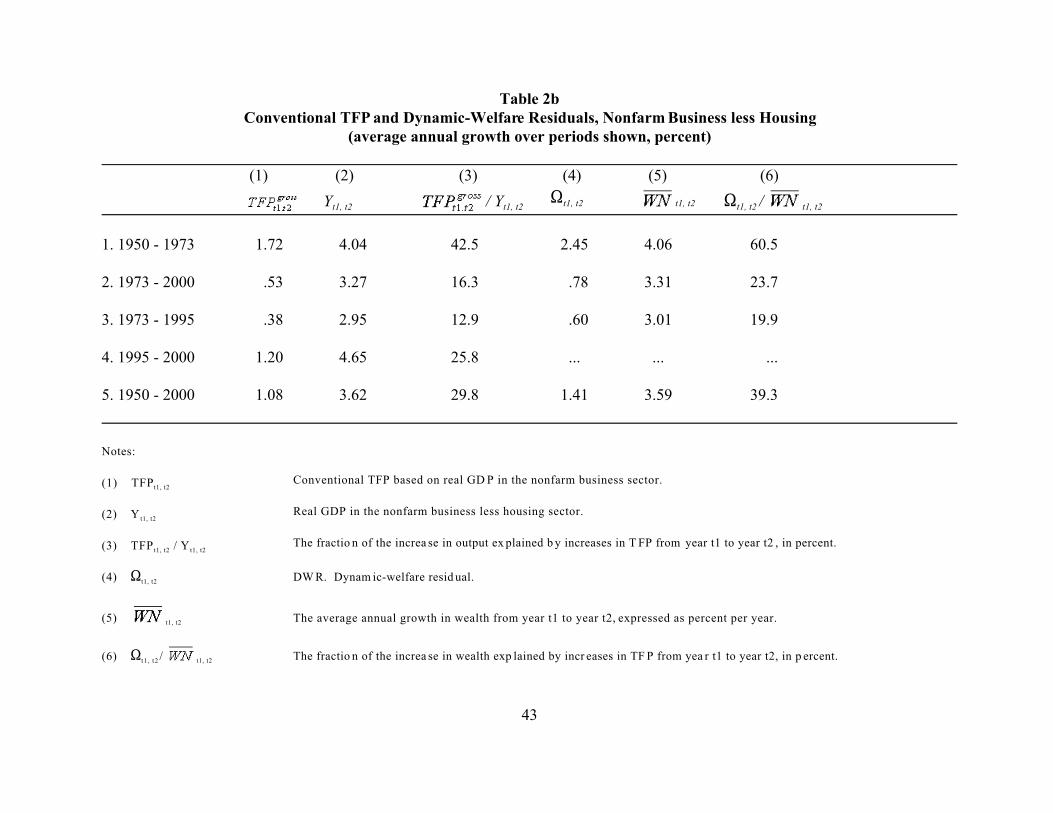
43

Table 2bConventional TFP and Dynamic-Welfare Residuals, Nonfarm Business less Housing

(average annual growth over periods shown, percent)

(1) (2) (3) (4) (5) (6)

Yt1, t2 / Yt1, t2St1, t2 t1, t2 St1, t2 / t1, t2

1. 1950 - 1973 1.72 4.04 42.5 2.45 4.06 60.5

2. 1973 - 2000 .53 3.27 16.3 .78 3.31 23.7

3. 1973 - 1995 .38 2.95 12.9 .60 3.01 19.9

4. 1995 - 2000 1.20 4.65 25.8 ... ... ...

5. 1950 - 2000 1.08 3.62 29.8 1.41 3.59 39.3

Notes:

(1) TFPt1, t2Conventional TFP based on real GD P in the nonfarm business sector.

(2) Y t1, t2Real GDP in the nonfarm business less housing sector.

(3) TFP t1, t2 / Y t1, t2The fractio n of the increa se in output ex plained b y increases in T FP from year t1 to year t2 , in percent.

(4) St1, t2 DW R. Dynam ic-welfare resid ual.

(5) t1, t2 The average annual growth in wealth from year t1 to year t2, expressed as percent per year.

(6) St1 , t2 / t1, t2 The fractio n of the increa se in wealth exp lained by incr eases in TF P from yea r t1 to year t2, in p ercent.

Table 3 Business Spending on Intangibles

TYPE OF ASSET OR SPENDING CATEGORY1

NIPA SNAESTIMATED SIZE (1998-2000 AVE.) AND COMMENTS

Computerized information: $ 140-165 billion

1. Computer software

(including expenses of software

developed for a firm’s own use)

I I BEA is further developing two of its three software

compo nents for the 20 03 revision . Census pro poses to

develop new survey measures of software spending.

2. Computerized databases C I Some po rtion of the de velopme nt costs are likely

captured in the NIP A computer so ftware measures.

Technology and innovative property: $ 200-300 billion

3. Science and engineering research

and development (“R&D”)

(costs of new products and new

production processes, usually leading

to a patent or license)

C C NSF data are available from the early 1950s and cover

work done in the physical scienc es, the biological sciences,

and engineering and computer science.2

(Mainly R&D in manufacturing and software

publishing industries; about $185 annually in 1998-2000)

4. Mineral exploration

(spending for the acquisition of new

reserves)

I I NIPA data do not include geological or geophysical

research.

(Mainly R&D in mining industries)

5. Copyright and license co sts

(spending for the development of

entertainment and artistic originals,

usually leading to a copyright or

license)

C I No broad statistical information.

The film indu stry capitalizes m ovie-makin g expense s in

financial reports.

(Mainly R&D in information industries, except software

publishers)

6. Other product development and

research ex penses (no t necessarily

leading to a p atent or cop yright)

C C No broad statistical information.

(Mainly R&D in finance and other services industries).

Econom ic competencies: $ 220-700 billion

7. Firm-specific human capital

(costs of developing wo rkforce skills,

i.e., on-the-job training and tuition

payments for job-related education)

C C A broad survey of emp loyers was co nducted b y BLS in

1994. S imilar surveys for since 199 6 were co nducted b y a

private research firm.

8. Organizational structure

(costs of organizational change and

development; company formation

expenses)

C C No broad statistical information, except employment and

wages by detailed occupational group. Value of executive

time can be estimated using these data.

Manageme nt consulting services.

9. Brand equity (advertising

expenditures and market research for

the development of brands and

trademarks)

C C Some, if not all, expenditures on advertising and market

research represent intermediate consumption.

Data by type of advertiser fro m 1935 on are ava ilable

from Universal McCann ($215 billion ave., 1998-2000)

1 C = Intermediate consumption; I = Investment; NIPA = U.S. National Income and Product Accounts; SNA = 1993

System of National Acc ounts.2 But excluding geophysical, geological, artificial intelligence, and expert systems research.

c

a

d b

Output/Labor

Capital/Labor0 k0 k1

A f(k )1 1

A f(k )0 0

q1

q0

q/

1

f

S

Figure 1

W

W

A Year 1C1

C2

0

B/

B

Year 2

U

U

b

a

U/

U/

Consumption in Years 1 and 2

Figure 2

45

References

Advisory Commission to Study the Consumer Price Index, Toward a More Accurate Measureof the Cost of Living, Final Report to the Senate Finance Committee, Washington D.C.,December 4, 1996.

Baily, Martin N. and Robert J. Gordon (1988). “Measurement Issues, the Slowdown, and theExplosion of Computer Power.” Brookings Papers on Economic Activity 2: 347-420.

Barro, Robert J. and Xavier Sala-i-Martin. 1995. Economic Growth. New York: McGraw-Hill.

Bartel, Ann (1991). “Employee Training Programs in U.S. Businesses.” in David Stern andJosef Ritzen, eds., Market Failure in Training: New Economic Analysis and Evidence onTraining of Adult Employees. Springer-Verlag.

Bartel, Ann (1994). “Productivity Gains from the Implementation of Employee TrainingPrograms.” Industrial Relations 33 (4):

Basu, Susanto, John G. Fernald, and Matthew D. Shapiro (2001). “Productivity Growth in the1990s: Technology, Utilization, or Adjustment?” Carnegie-Rochester ConferenceSeries on Public Policy 55: 117-165.

Berndt, Ernest R. and Melvyn A. Fuss (1986). “Productivity Measurement With Adjustmentsfor Variations in Capacity Utilization and Other Forms of Temporary Equilibrium.” Journal of Econometrics 33: 7-29.

Black, Sandra and Lynch, Lisa M. (1996). “Human Capital Investments and Productivity.”American Economic Review 86 (2, May): 263-267.

Blair, Margaret M. and Steven M.H. Wallman (2000). “Unseen Wealth: Report of theBrookings Task Force on Understanding Intangible Sources of Value.” Washington,D.C.: Brookings Institution.

Brynjolfsson, E. and Yang, S. (1999). “The Intangible Costs and Benefits of ComputerInvestments: Evidence from the Financial Markets.” Atlanta, Georgia: Proceedings ofthe International Conference on Information Systems.

Brynjolfsson, E., Hitt, L., and Yang, S. (2000). “Intangible Assets: How the Interaction ofInformation Technology and Organizational Structure Affects Stock MarketValuations.” Cambridge, Mass: MIT Working paper.

Cass, David (1965). “Optimum Growth in an Aggregative Model of Capital Accumulation.” Review of Economic Studies 32 (July): 233-240.

Cockburn, Iian and Zvi Griliches (1988). “Industry Effects and Appropriability Measures in the

46

Stock Market's Valuation of R&D and Patents.” American Economic Review 78 (2,May): 419-123.

Corrado, Carol and Larry Slifman (1999). “A Decomposition of Productivity and Costs.” Amerian Economic Review 89 (2, May): 328-332.

Denison, Edward F. (1962). The Sources of Economic Growth in the United States and theAlternatives Before Us. New York: Committee for Economic Development.

Denison, Edward F. (1964). “The Unimportance of the Embodiment Question.” AmericanEconomic Review 79 (5): 90-94.

Domar, Evsey D. (1961). “On the Measurement of Technical Change.” Economic Journal 71:710-729.

Domar, Evsey D. (1963). “Total Factor Productivity and the Quality of Capital.” Journal ofPolitical Economy 71 (December): 586-588.

Fraumeni, Barbara M. (2000). “The Output of the Education Sector as Determined byEducation’s Effect on Lifetime Income.” Presented at Workshop on Measuring theOutput of the Education Sector. Washington, D.C.: Brookings Institution. Available at

http://www.brookings.edu/es/research/projects/productivity/workshops/2000040704.pdf

Gordon, Robert J. (2002). “Technology and Economic Performance in the AmericanEconomy.” National Bureau of Economic Research working paper # 8771.

Greenwood, Jeremy, Zvi Hercowitz, and Per Krusell (1997). “Long-Run Implications ofInvestment-Specific Technical Change.” American Economic Review 87 (3, June): 342-362.

Griliches, Zvi (1973). “Research Expenditures and Growth Accounting.” In B.R. Williams,ed., Science and Technology in Economic Growth, The Price Statistics of the FederalGovernment, MacMillan Press.

Griliches, Zvi (1981). “Market Value, R&D and Patents.” Economic Letters 7: 183-87.

Griliches, Zvi (1994). “Productivity, R&D, and the Data Constraint.” American EconomicReview 84 (1, March): 1-23.

Griliches, Zvi (1996). “The Discovery of the Residual: A Historical Note.” Journal ofEconomic Literature 34 (September): 1324-1330.

Grossman, Gene M. and Elhanan Helpman (1991). Innovation and Growth in the GlobalEconomy. Cambridge, Massachusetts: MIT Press.

47

Hall, Bronwyn H. (1993). “The Stock Market Value of R&D Investment During the 1980s.” American Economic Review 83 (May): 259-64.

Hall, Bronwyn H. and Robert E. Hall (1993). “The Value and Performance of U.S.Corporations.” Brookings Papers on Economic Activity (1993,1): 1-34.

Hall, Robert E. and Dale W. Jorgenson (1967). “Tax Policy and Investment Behavior.”American Economic Review 57: 391-414.

Hall, Robert E (1968). “Technical Change and Capital From the Point of View of the Dual.”Review of Economic Studies 35: 34-46.

Hall, Robert E. (2000a). “e-Capital: The Link between the Stock market and th Labor Market inthe 1990s.” Brookings Papers on Economic Activity (2000,2):

Hall, Robert E. (2001). “Struggling to Understand the Stock Market.” The 2001 Ely Lecture.(January).

Hulten, Charles R. (1978). “Growth Accounting with Intermediate Inputs.” Review ofEconomic Studies 45 (October): 511-518.

Hulten, Charles R. (1979). “On the ‘Importance’ of Productivity Change.” American EconomicReview 69: 126-136.

Hulten, Charles R. (1992a). “Accounting for the Wealth of Nations: The Net versus GrossOutput Controversy and its Ramifications.” Scandinavian Journal of Economics 94(supplement): S9-S24.

Hulten, Charles R. (1992b). “Growth Accounting when Technical Change is Embodied inCapital.” American Economic Review 82 (4, September): 964-980.

Hulten, Charles R. (1996). “Quality Change in Capital Goods and its Impact on EconomicGrowth.” National Bureau of Economic Research Working Paper 5569.

Hulten, Charles R. and Frank C. Wykoff (1981). “The Estimation of Economic DepreciationUsing Vintage Asset Prices.” Journal of Econometrics 15: 367-396.

Jorgenson, Dale W. (1963). “Capital Theory and Investment Behavior.” American EconomicReview 53 (2, May): 247-259.

Jorgenson, Dale W. (1966). “The Embodiment Hypothesis.” Journal of Political Economy 74(February): 1-17.

Jorgenson, Dale W. and Barbara M. Fraumeni (1989a). “The Accumulation of Human andNonhuman Capital, 1948-84.”In Robert E. Lipsey and Helen Stone Tice, eds., The

48

Measurement of Saving, Investment, and Wealth, Studies in Income and Wealth Number52. Chicago: Chicago University Press for the NBER: 119-152.

Jorgenson, Dale W. and Barbara M. Fraumeni (1992). “The Output of the Education Sector.”In Zvi Griliches (ed.), Output Measurement in the Service Sectors, Studies in Incomeand Wealth, Number 56. Chicago: Chicago University Press for the NBER: 303-341.

Jorgenson, Dale W. and Zvi Griliches (1967). “The Explanation of Productivity Change.”Review of Economic Studies 34 (July): 349-83.

Jorgenson, Dale W. and Zvi Griliches (1972). “Issues in Growth Accounting: A Reply toEdward F. Denison.” Survey of Current Business 52: 65-94.

Jorgenson, Dale W. and Kevin J. Stiroh (2000). “U.S. Economic Growth in the NewMillenium.” Brookings Papers on Economic Activity 1, pp. 125-211.

Jorgenson, Dale W., Mun S. Ho, and Kevin J. Stiroh (2002). “Information Technology,Education, and the Sources of Economic Growth across U.S. Industries.”Washington,D.C.: Measuring Capital in the New Economy, Conference on Research on Income andWealth.

Kaplan, M.C. (1987). “Intangible Investment: An Essay at International Comparison.” Paris:Memorandum to the OECD Industry Committee.

Khan, Mosahid (2001). “Investment in Knowledge.” Paris: OECD Directorate for Science,Technology and Industry working paper.

Kiley, Michael T. (2001). “Computers and Growth with Frictions: Aggregate and DisaggregateEvidence. Carnegie-Rochester Conference Series on Public Policy 55: 171-215.

Koopmans, T.C. (1965). “On the Concept of Optimal Economic Growth.” Pacifica. Rome:Academia Scientiarus: 276-279.

Lebow, David E., John M. Roberts, and David J. Stockton (1994). “Monetary Policy and ‘ThePrice Level’.” Mimeo, Board of Governors of the Federal Reserve System.

Lev, Baruch – one or two of his earlier pieces.

Lev, Baruch (2001). Intangibles: Management, Measurement, and Reporting. Washington,D.C.: Brookings Institution.

Lucas, Robert E. Jr. (1988). “On the Mechanics of Economic Development.” Journal ofMonetary Economics 22: 3-42.

McGratten, Ellen and Edward C. Prescott (2000). “Is the Stock Market Overvalued?” Federal

49

Reserve Bank of Minneapolis Quarterly Review (24:4 Fall): 20-40.

McGuckin, Robert (1994).

Moylan, Carol (2001). “Estimation of Software in the U.S. National Accounts: NewDevelopments.” Paris: OECD Statistics Directorate.

Nakamura, Leonard (1999). “Intangibles: What Put the New in the New Economy?” FederalReserve Bank of Philadelphia Business Review (July/August): 3-16.

Nakamura, Leonard (2000). “Economics and the New Economy: The Invisible Hand MeetsCreative Destruction.” Federal Reserve Bank of Philadelphia Business Review(July/August): 15-30.

Nakamura, Leonard (2001). “What is the US Gross Investment in Intangibles? (At Least) OneTrillion Dollars a Year!” Federal Reserve Bank of Philadelphia Working Paper No. 01-15.

Nordhaus, William D., and Edward C. Kokkelenberg, eds. (1999). Nature's Numbers,Expanding the National Economic Accounts to Include the Environment. Washington,D.C.: National Academy Press for the National Research Council.

OECD Secretariat (1998). “Measuring Intangible Investment: Selected Bibliography.”Available at http://www1.oecd.org/dsti/sti/industry/indcomp/prod/paper16.pdf.

Oliner, Stephen D. and Daniel E. Sichel (2000). “The resurgence of growth in the late 1990s:Is information technology the story?” Journal of Economic Perspectives 14, Fall: 3-22.

Oliner, Stephen D. and Daniel E. Sichel (2002). “Information Technology and Productivity:Where are We Now and Where are We Going?” forthcoming, Atlanta Fed Review.

Parker, Robert and Bruce Grimm (1999). “Recognition of Business and GovernmentExpenditures for Software as Investment: Methodology and Quantitative Impacts, 1959-98.” Bureau of Economic Analysis. Available at BEA website.

Prucha, Ingmar R., and M. Ishaq Nadiri (1981). “Endogenous Capital Utilization andProductivity Measurement in Dynamic Factor Demand Models: Theory and anApplication to the U.S. Electrical Machinery Industry.” Journal of Econometrics 15:367-396.

Romer, Paul M. (1986). “Increasing Returns and Long-Run Growth.” Journal of PoliticalEconomy 94 (5): 1002-1037.

Romer, Paul M. (1990). “Endogenous Technical Change.” Journal of Political Economy 98(5): 71-102.

50

Rymes, Thomas K. (1971). On Concepts of Capital and Technical Change. Cambridge, U.K.: Cambridge University Press.

Solow, Robert M. (1956). “A Contribution to the Theory of Economic Growth.” QuarterlyJournal of Economics 70 (February): 65-94.

Solow, Robert M. (1957). “Technical Change and the Aggregate Production Function.” Review of Economics and Statistics 39 (August): 312-320.

Solow, Robert M. (1960). “Investment and Technical Progress.” in K. Arrow, S. Karlin and P.Suppes, eds., Mathematical Methods in the Social Sciences. Stanford: StanfordUniversity Press.

Swan, T.W. (1956). “Economic Growth and Capital Accumulation.” The Economic RecordXXXII: 334-361.

System of National Accounts 1993. Commission of the European Communities, InternationalMonetary Fund, Organization for Economic Co-operation and Development, UnitedNations, and World Bank.

Tice, Helen S. (1991). “Report of the Proceedings.” Workshop on the Revision of the U.N.System of National Accounts, Conference on Research in Income and Wealth,November 9, 1990, Washington D.C.

Triplett, Jack E. (1983). “Concepts of Quality in Input and Output Price Measures: AResolution of the User Value-Resource Cost Debate.” in Murray F. Foss, ed., The U.S.National Income and Product Accounts: Selected Topics, Studies in Income andWealth, Number 47, Chicago: University of Chicago Press for the NBER: 296-311.

Triplett, Jack E. (1999). “ ” Business Economics.

U.S. Department of Labor, Bureau of Labor Statistics. (1983). Trends in MultifactorProductivity, 1948-81. Washington D.C.: US GPO Bulletin 2178.

Vosselman, Wim (1992). “Initial Guidelines for the Collection and Comparison of Data onIntangible Investment.” Paper prepared at the OECD Workshop on the Measurement ofIntangible Investment. Paris: OECD. Available athttp://www1.oecd.org/dsti/sti/industry/indcomp/prod/intang.htm.

Weitzman, Martin L. (1976). “On the Welfare Significance of National Product in a DynamicEconomy.” The Quarterly Journal of Economics 90: 156-162.

Wolff, Edward, N. (1996). “The Productivity Slowdown: The Culprit At Last? Follow-up onHulten and Wolff.” American Economic Review 86 (5, December): 1239-1252.