measuring and quantifying driver workload on limited
TRANSCRIPT

Measuring and Quantifying Driver Workload on Limited Access Roads
by
Ke Liu
A dissertation submitted in partial fulfillment
of the requirements for the degree of
Doctor of Philosophy
(Industrial and Operations Engineering)
in The University of Michigan
2019
Doctoral Committee:
Research Professor Paul Green, Co-Chair
Professor Yili Liu, Co-Chair
Professor Richard Gonzales
Professor Nadine Sarter
Assistant Professor Jessie Xi Yang


ii
DEDICATION
This dissertation is dedicated to the readers.

iii
ACKNOWLEDGMENTS
This work was financially supported by the fellowship and Graduate Student Instructor
positions (IOE 333 and IOE 334) provided by the Department of Industrial and Operations
engineering (IOE) at the University of Michigan, M. Scheller Fellowship by the College of
Engineering at the University of Michigan, and Patricia F. Waller Scholarship by the University
of Michigan Transportation Research Institute (UMTRI).
I would like to thank my advisors Dr. Paul Green and Dr. Yili Liu for guiding me and
sharing their knowledge with me; my dissertation committee members Dr. Richard Gonzales, Dr.
Nadine Sarter, and Dr. Jessie Yang for their comments and suggestions; my peers at IOE
department for their help and encouragement; the faculties and staff members at IOE and
UMTRI, especially Dr. Clive D’Souza, Charles Woolley, Dr. Sheryl Ulin, Dr. Brian Lin,
Christopher Konrad, Matt Irelan, Tina Picano Sroka, Teresa Maldonado, Karen Alexa, Diane
Elwart for their help and support.
Lastly, I would like to thank my parents, my husband, and my daughter for their
unconditional love and support.

iv
TABLE OF CONTENTS
DEDICATION............................................................................................................................... ii
ACKNOWLEDGMENTS ........................................................................................................... iii
LIST OF TABLES ...................................................................................................................... vii
LIST OF FIGURES ................................................................................................................... viii
ABSTRACT ................................................................................................................................... x
CHAPTER 1
Introduction ................................................................................................................................... 1
1.1 Motivation ............................................................................................................................ 1
1.2 Mental Workload ................................................................................................................ 4
1.3 Measurements of Workload ............................................................................................... 6
1.4 Overview of the Chapters ................................................................................................. 10
References ................................................................................................................................ 12
CHAPTER 2
A Workload Model ..................................................................................................................... 16
2.1 Hypothesis .......................................................................................................................... 16
2.2 A Workload Model for Static Conditions ....................................................................... 19
2.3 A Workload Model for Dynamic Conditions .................................................................. 22
References ................................................................................................................................ 25
CHAPTER 3
An Experimental Investigation of How Static Traffic Affects Driver Workload ................. 26
3.1 Introduction ....................................................................................................................... 26
3.2 Methods .............................................................................................................................. 26
3.2.1 Participants ................................................................................................................... 26
3.2.2 Workload measures and experiment design ................................................................. 27
3.2.3 Experiment setup .......................................................................................................... 29
3.2.4 Procedure ...................................................................................................................... 30

v
3.2.5 Statistical analysis......................................................................................................... 31
3.3 Results ................................................................................................................................ 32
3.3.1 Categorizations of scenarios (question 3.1) .................................................................. 32
3.3.2 Anchored rating (questions 3.2, 3.3) ............................................................................ 33
3.3.3 Occlusion% (questions 3.2, 3.3) ................................................................................... 41
3.3.4 Performance (questions 3.2, 3.3) .................................................................................. 46
3.4 Discussion ........................................................................................................................... 47
3.4.1 Categorization of driving scenarios (question 3.1) ....................................................... 47
3.4.2 Relationship between Distance Headway (DHW) and workload measures (question
3.2) ......................................................................................................................................... 48
3.4.3 The Model using Time Headway (THW) to predict workload (question 3.3) ............. 49
3.4.4 Differences between workload measures (question 3.4) .............................................. 50
References ................................................................................................................................ 52
CHAPTER 4
An Experimental Investigation of How Dynamic Traffic Affects Driver Workload ............ 53
4.1 Introduction ....................................................................................................................... 53
4.2 Methods .............................................................................................................................. 54
4.2.1 Participants ................................................................................................................... 54
4.2.2 Workload measures and experiment design ................................................................. 54
4.2.3 Experiment Setup ......................................................................................................... 55
4.2.4 Procedure ...................................................................................................................... 56
4.2.5 Statistical Analysis ....................................................................................................... 57
4.3 Results ................................................................................................................................ 57
4.3.1 The effects of traffic elements on anchored rating (question 4.1) ................................ 57
4.3.2 The effects of traffic elements on occlusion% (question 4.1) ...................................... 62
4.3.3 The effects of traffic elements on performance (question 4.1) ..................................... 66
4.3.4 The effects of continuous set on workload measures (question 4.2) ............................ 70
4.4 Discussion ........................................................................................................................... 71
4.4.1 Effects of traffic elements on workload (question 4.1) ................................................ 71
4.4.2 Workload model determined by THW and Time to Collision (TTC) (question 4.2) ... 72
4.4.3 Differences among workload measures (question 4.3) ................................................ 72
CHAPTER 5
GOMS Modeling of Driver Workload in Static and Dynamic Traffic .................................. 75
vi
5.1 Introduction ....................................................................................................................... 75
5.2 Methods .............................................................................................................................. 76
5.3 Results ................................................................................................................................ 85
5.4 Discussion ........................................................................................................................... 87
References ................................................................................................................................ 89
CHAPTER 6
Conclusions .................................................................................................................................. 90
6.1 Dissertation Summary ...................................................................................................... 90
6.2 Conclusions ........................................................................................................................ 92
6.2.1 The effects of DHW on workload in static traffic ........................................................ 92
6.2.2 The effects of traffic elements on workload in dynamic traffic ................................... 92
6.2.3 The workload model ..................................................................................................... 92
6.2.4 The differences among workload measures ................................................................. 93
6.2.5 The GOMS model ........................................................................................................ 93
6.3 Contributions to Current Knowledge ............................................................................. 94
6.4 Future Research ................................................................................................................ 94
6.4.1 The workload model ..................................................................................................... 94
6.4.2 Differences among workload measures ........................................................................ 95
6.4.3 Incorporate the workload model into other driving studies .......................................... 95
vii
LIST OF TABLES
Table 1.1 Previous take-over studies did not consider workload induced by traffic ...................... 3
Table 2.1 Illustration of basic scenarios (static conditions) .......................................................... 20
Table 2.2 Workload modeling based on THW in static conditions .............................................. 21
Table 2.3 Illustration of basic scenarios (dynamic conditions) .................................................... 23
Table 3.1 The levels of THW to be examined .............................................................................. 28
Table 3.2 The number of cases to be examined in each scenario (stable condition) .................... 29
Table 3.3 Correlations between performance statistics and workload rating ............................... 33
Table 3.4 P values for post-hoc comparisons between all scenario types (rating) ....................... 34
Table 3.5 The main effects of DHWs on workload rating in different scenarios ......................... 35
Table 3.6 Regression equations in different scenarios (Rating) ................................................... 41
Table 3.7 P values for post-hoc comparisons between all scenario types (occlusion%) .............. 42
Table 3.8 The main effects of DHWs on occlusion% in different scenarios ................................ 42
Table 3.9 Regression equations for different scenarios (occlusion%) .......................................... 46
Table 3.10 the effects of DHWs on performance statistics .......................................................... 46
Table 3.11 Regression equations for different scenarios (performance statistics) ....................... 47
Table 4.1 The number of cases examined in dynamic traffic. ...................................................... 55
Table 4.2 The effects of traffic elements on workload ratings ..................................................... 58
Table 4.3 The effects of traffic elements on occlusion% .............................................................. 62
Table 4.4 The relationship between performance statistics and anchored rating ......................... 67
Table 4.5 The effects of traffic elements on performance statistics ............................................. 67
Table 4.6 Coefficients for possible regression equations and corresponding p values ................ 71

viii
LIST OF FIGURES
Figure 2.1 Definition of distance headway and gap used in this study: (a) when two vehicles are
on the same lane and (b) when two vehicles are on different lanes. ............................................. 17
Figure 2.2 TTC and THW are possibly closely related to workload ............................................ 18
Figure 3.1 Driving Simulator Set up ............................................................................................. 30
Figure 3.2 Anchor clips for subjective rating ............................................................................... 31
Figure 3.3 Driver workload ratings at different DHW levels in 8 tested scenarios ...................... 38
Figure 3.4 Driver workload ratings at different DHW levels in all scenarios .............................. 39
Figure 3.5 Driver workload ratings in four scenarios (S1, S3, S7, S8) ........................................ 40
Figure 3.6 Driver workload ratings in four scenarios (S4, S6, S7, S8) ........................................ 40
Figure 3.7 (S1) occlusion% contributed by a lead vehicle (S2) occlusion% contributed by both
lead and following vehicles .......................................................................................................... 43
Figure 3.8 Occlusion% in S7 ........................................................................................................ 44
Figure 3.9 Occlusion% in S8 ........................................................................................................ 44
Figure 3.10 Occlusion% at different DHW level in all scenarios ................................................. 45
Figure 3.11 Occlusion% in four scenarios (S1, S3, S7, S8) ......................................................... 45
Figure 3.12 The effects of DHWs on SDS(mph) and SDSTW(degree) in S8 .............................. 47
Figure 4.1 The comparison between workload ratings in different lanes (faster/slower) ............ 58
Figure 4.2 The comparison among workload ratings with different relative velocities ............... 59
Figure 4.3 The comparison among workload ratings with different lane change actions ............ 59
Figure 4.4 Interaction effect between relative velocity and lane on ratings ................................. 60
Figure 4.5 Interaction effect between lane change urgency and lane on ratings .......................... 61
Figure 4.6 Interaction effect between relative velocity and lane change urgency on ratings ....... 61
Figure 4.7 The comparison between occlusion% in different lanes (faster/slower) ..................... 63
Figure 4.8 The comparison among occlusion% with different relative velocities. ...................... 63
Figure 4.9 The comparison among occlusion% with different lane change events ...................... 64
Figure 4.10 Interaction effect between relative velocity and lane on occlusion% ....................... 64

ix
Figure 4.11 Interaction effect between lane change action and lane on occlusion% ................... 65
Figure 4.12 Interaction effect between relative velocity and lane change urgency on occlusion%
....................................................................................................................................................... 66
Figure 4.13 The main effects of block on performance statistics ................................................. 68
Figure 4.14 The main effects of lane change urgency on performance statistics ......................... 69
Figure 4.15 The main effects of relative velocity on performance statistics ................................ 69
Figure 4.16 The interaction effect of relative velocity and lane on performance statistics .......... 70
Figure 4.17 The interaction effect of lane change action and lane on some performance statistics
....................................................................................................................................................... 70
Figure 5.1 A Flow Chart of the Workload Rating Task ............................................................... 77
Figure 5.2 NGOMSL-Style Description of the Workload Rating Task in Static Traffic ............. 80
Figure 5.3 NGOMSL-Style Description of the Workload Rating Task in Dynamic Traffic ....... 84
Figure 5.4 Workload rating comparisons between the GOMSL model and experimental results in
static traffic (Assumption: all the vehicles are equally important) ............................................... 85
Figure 5.5 Workload rating comparisons between the GOMS model and experimental results in
static traffic (Assumption: vehicles are not equally important by assigning weighting factors to
different vehicles) ......................................................................................................................... 86
Figure 5.6 Workload rating comparisons between the GOMS model and experimental results in
dynamic traffic (IDV: lane) .......................................................................................................... 86
Figure 5. 7 Workload rating comparisons between the GOMS model and experimental results in
dynamic traffic (IDV: relative velocity) ....................................................................................... 87
Figure 5. 8 Workload rating comparisons between the GOMS model and experimental results in
dynamic traffic (IDV: the urgency of lane change action) ........................................................... 87

x
ABSTRACT
Minimizing driver errors should improve driving safety. Driver errors are more common
when workload is high than when it is low. Thus, it is of great importance to study driver
workload. Knowing the amount of workload at any given time, take-over time can be
determined, adaptive in-vehicle systems can be refined, and distracting in-vehicle secondary
tasks can be regulated.
In this dissertation, a model quantifying workload as a function of traffic, in which
workload is proportional to inverse time headway (THW) and time to collision (TTC), was
proposed. Two experiments were conducted to investigate how traffic affected driver workload
and evaluate the proposed model. The driving scenarios were categorized into static (i.e., no
relative movements among vehicles) and dynamic (i.e., there are relative velocities and lane
change actions). Three categories of workload measures (i.e., workload rating, occlusion %, and
driving performance statistics) were analyzed and compared. A GOMS model was built based
upon a timeline model by using timerequired to represent mental resources demanded and
timeavailable to represent mental resources available.
In static traffic, the workload rating increased with increased number of vehicles around
but was unaffected by participant age. The workload ratings decreased with increasing Distance
Headways (DHWs) of each vehicle. From greatest to least, the effects were: DHWLead,
DHWLeftLead, DHWLeftFollow, DHWFollow. Any surrounding vehicle that was 14.5 m away from the
participant resulted in significant greater workload. Drivers tended to compromise longitudinal

xi
speed but still maintain lateral position when workload increased. Although occlusion% was less
sensitive to scenarios having no lead vehicles, it can nonetheless be well predicted using the
proposed workload model in sensitive scenarios. The resulting equations were occlusion% = 0.35
+ 0.05/THWLead + 0.02/THWLeftLead - 0.08Age (Rocclusion2=0.91); rating = 1.74 + 1.74/THWLead +
0.20/THWFollow + 0.79/THWLeftLead + 0.28/THWLeftFollow (Rrating2=0.73). In dynamic traffic, drivers
experienced greater workload in the faster lane; higher workload level was associated with
greater relative velocity between two lanes. Both rating and occlusion% can be described using
the proposed model: Anchored rating = 4.53 + 1.215/THWLeftLeadLead + 0.001/THWLeftFollow +
3.069/THWLeadLead + 0.524/THWLead + 0.240/(TTCLead×TTCLeadLateral) +
30.487/(TTCLeftLead×TTCLeftLeadLateral) (Rrating2=0.54); Occlusion% = 0.381 + 0.150/THWLeftLeadLead
˗ 0.117/THWLeadLead + 0.021/THWLead + 2.648/(TTCLeftLead×TTCLeftLeadLateral) (Rocclusion2=0.58). In
addition, it was shown that the GOMS model accounted for the observed differences of workload
ratings from the empirical data (R2>0.83).
In contrast to most previous studies that focus on average long-term traffic statistics (e.g.,
vehicles/lane/hour), this dissertation provided equations to predict two measures of workload
using real-time traffic. The comparisons among three workload measures provided insights into
how to choose the desired workload measures in their future research. In GOMS model, the
procedural knowledge of rating workload while driving was developed. They should be
transferrable to other workload studies and can serve as the primary tool to justify experimental
design.
Scientifically, the results of this dissertation offer insights into the mechanism of the way
that humans perceive workload and the corresponding driving strategies. From the engineering
application and practical value perspective, the proposed workload model would help future

xii
driving studies by providing a way to quantify driver workload and support the comparison of
studies in different situations.

1
CHAPTER 1
Introduction
1.1 Motivation
According to the World Health Organization (WHO), more than 1.2 million people die
on the world’s roads each year, and as many as 50 million others are injured (World Health
Organization, 2009). More than 30,000 people die in crashes on U.S. roadways each year
(National Highway Traffic Safety Administration, 2014). From 2014 to 2015, the increase in the
number of people who died in crashes was the largest percentage increase (7.2%) in the past 50
years (National Highway Traffic Safety Administration, 2016). How to reduce driving deaths is
an important issue in transportation research.
Driver error has been found to be the main cause of 45% to 75% of crashes (Wierwille et
al., 2002). Driving under high workload can result in increased driver errors (Hancock et al.,
1990; Briggs et al., 2011). In addition, prolonged exposure to high workload degrades driver
performance (Strayer and Johnston, 2001; Engstrom et al., 2005; Fuller, 2005). Thus, driver
workload is an important factor that affects the interactions between vehicles and drivers.
Workload discussed in this dissertation refers to mental/cognitive workload. (Physical
workload, which is commonly measured using energy expenditure rates, is not of interest here).
Mental workload can be described as “the relation between the function relating the mental
resources demanded by a task and those resources available to be supplied by the human
operator” (Parasuraman et al., 2008). If either mental resources needed or resources supplied

2
changes, then workload changes. The concept of workload is valuable as it shows the distinctions
between different operators are working on the same task and the same operator is working on
different tasks.
Workload can be affected by activities from both inside and outside of the vehicles.
Inside of vehicles, different activities (e.g., cell phone use, adaptive cruise control) were found to
increase driver workload (Ma and Kaber, 2005). Turn maneuvers resulted in significant increase
in driver workload (Hancock et al., 1990). Outside of the vehicles, curve radius significantly
affected driver workload (Tsimhoni and Green, 1999). Weather has been widely examined in
terms of its relationship with driver workload. A significant increase in driver workload was
observed when wind gust was placed at the front of the vehicle compared to gust towards the
center of the vehicles (Hicks and Wierwille, 1979). Driver workload in fog was significant
higher compared to normal visibility (Hoogendoorn et al., 2011).
Besides the outside factors mentioned above, surrounding traffic is one of the most
important factors and has not been systematically varied and examined. Previous research
examining the effect of traffic on workload either lacked a quantitative definition of traffic (Jahn
et al., 2005; Patten et al., 2006; Cantin et al., 2009) or provided no real-time spatial dimensions
for the surrounding vehicles (Teh et al., 2014). No one has made a connection between real-time
traffic and workload. The following three examples show necessity of the model relating real-
time traffic to quantified workload.
In take-over studies (take-over refers to the transfer of control between manual driving
and automated driving), workload should be quantified. In previous take-over studies, take-over
timing and its effects were studied with little consideration of workload contributed by
surrounding traffic (Table 1.1). Research showed that workload resulting from surrounding

3
vehicles affected take-over time (Radlmayr et al., 2014). Thus, results from take-over studies
without considering workload contributed by real-time raffic are less convincing.
Table 1.1 Previous take-over studies did not consider workload induced by traffic
Study Tasks Main Findings Limitations
Gold et al.,
2013
Take over request (TOR) time (7s
vs. 5s) was assessed in take-over
scenarios compared to manual
driving. A secondary task added
workload in the worst case scenario.
Shorter take-over time
resulted in faster
reactions but worse
quality (utilization of
acceleration potential).
No traffic in take-over
scenarios. There was no
traffic on adjacent lane.
Mok et al.,
2015
Three transition time conditions
were tested (2s, 5s, or 8s before
encountering a road hazard). A
secondary task added workload in
the worst case scenario.
The minimum
transition time for take-
over should be between
2s to 5s.
No traffic was provided
during take-overs. Only
oncoming traffic was
shown after the alert to
keep drivers to stay in
assigned lanes.
Clark et
al.,
2015
The effectiveness of two take-over
warnings were examined (warning
given 7.5s or 4.5s before take-over).
The longer warning
(7.5s) leads to better
control over lane
position at take-over.
No traffic was provided
when studying take-
over warnings.
Radlmayr
et al., 2014
Take-over time was evaluated in 4
traffic situations (1 traffic condition
vs. 3 no traffic conditions) and
secondary tasks.
Both traffic situation
(p=0.01) and secondary
task (p=0.02) had a
significant impact on
take-over time.
Only one traffic
situation was studied.
No quantitative
description of traffic
was provided.
Quantifying driver workload as a function of traffic could help contribute to the design of
adaptive in-vehicle systems (e.g., a workload estimator: an adaptive man-machine interface that
filters information needed according to situational requirements to avoid overload). In
Piechulla’s research (2003), a real-time workload estimator was implemented to redirect
incoming telephone calls to a mailbox whenever workload exceeded a threshold value. The
research showed that workload can be reduced by using a workload estimator to manage
distraction (i.e., route calls when workload is high, thereby reducing distraction). However, the
workload estimator was established mainly based on driver performance after experiencing
different traffic scenarios. In reality, the temporal workload and performance are not changing
simultaneously (explanations can be found in Chapter 1.3 in this dissertation). In Verwey’s

4
research (2000), the road situation was identified as a critical factor for driver workload
estimation. However, road situations were described only qualitatively (e.g., standing still at
traffic light). The lack of unified and systematic descriptions of traffic scenarios severely hinders
the development of workload estimators.
Quantifying driver workload as a function of traffic would benefit regulating secondary
tasks as well. Many studies have found some in-vehicle secondary tasks should be prohibited
while driving (Strayer and Johnston, 2001; Horberry et al., 2006; Kass et al., 2007; Collet et al.,
2009). But what levels of secondary task are excessively distracting should depend on the
workload of the primary driving task. For example, if the primary driver workload is low (e.g.,
no cars around, 4 straight lanes in each direction), then drivers should have the capacity to deal
with secondary tasks.
In sum, measuring and quantifying workload in terms of real-time traffic enhances
driving safety by providing adequate take-over time, refining adaptive in-vehicle systems, and
regulating in-vehicle secondary tasks.
1.2 Mental Workload
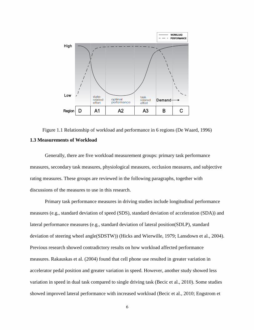
A relationship among mental workload, task performance, and task demands was
proposed by De Waard (1996). First of all, workload and task demands are different concepts:
workload reflects the individual reaction to task demands (Figure 1.1). In regions of the task
demand A1, A2, A3, performance remains stable and is independent of task demands. At region
A2, operators can easily deal with driving tasks and can maintain performance at a stable level
with increasing demands. Task demand can shift from region A2 towards region D/C due to
decreased driver state (driver state can be affect by monotony, fatigue, sedative drugs, and
alcohol) or increased task complexity. From region A2 to A1, drivers experience a reduced state:

5
workload is increased but performance can be maintained. If drivers’ state keep deteriorating,
workload will keep increasing and performance will decrease (region D). From region A2 to A3,
drivers are able to maintain performance by increasing effort. One side effect associated with
region A3 is increased performance, as drivers are trying to exert extra effort. In region B,
performance degrades with increasing task demand. In region C, performance is at its minimum
level regardless of task demands.
As the driver workload contributed by traffic is of interest, the most important regions
that need to be explored are regions A3 and B (due to increased task complexity). In region A3,
performance can be maintained but workload is increasing. Thus, performance can be used to
categorize tasks into region A3 and B: if performance decreases when workload increases, then
the task demand falls in region B; otherwise, the task demand falls in region A3. Furthermore,
performance cannot serve as a sensitive workload measure in region A3. When a workload
estimator is developed using performance (Piechulla, 2003), then it has already lost its time-
sensitive property. Watching workload variations closely in region A3 before performance
change is critical.
Knowing this relationship, one can categorize task demands into regions by the
relationship between workload and performance. By knowing the task demands’ regions, it is
easy to determine whether it’s proper to use performance statistics to indicate the workload level.
6
Figure 1.1 Relationship of workload and performance in 6 regions (De Waard, 1996)
1.3 Measurements of Workload
Generally, there are five workload measurement groups: primary task performance
measures, secondary task measures, physiological measures, occlusion measures, and subjective
rating measures. These groups are reviewed in the following paragraphs, together with
discussions of the measures to use in this research.
Primary task performance measures in driving studies include longitudinal performance
measures (e.g., standard deviation of speed (SDS), standard deviation of acceleration (SDA)) and
lateral performance measures (e.g., standard deviation of lateral position(SDLP), standard
deviation of steering wheel angle(SDSTW)) (Hicks and Wierwille, 1979; Lansdown et al., 2004).
Previous research showed contradictory results on how workload affected performance
measures. Rakauskas et al. (2004) found that cell phone use resulted in greater variation in
accelerator pedal position and greater variation in speed. However, another study showed less
variation in speed in dual task compared to single driving task (Becic et al., 2010). Some studies
showed improved lateral performance with increased workload (Becic et al., 2010; Engstrom et

7
al., 2005), whereas there is research showing greater workload was associated with decreased
lateral performance (Engstrom et al., 2005; Strayer and Johnstom, 2001). Some research showed
there was no association between workload and lateral performance measures (Alm and Nilsson,
1995; Rakauskas et al., 2004). There are many contradictory results, which can be explained
using the relationship between workload and performance mentioned in section 1.2. Performance
is sensitive to workload in region B (higher workload) whereas performance is not sensitive to
workload in region A3 (lower workload). But primary task performance measures are still
important in workload study for two reasons (De Warrd, 1996): (1) reduced primary task
performance can indicate overload; (2) improved primary task performance can be due to
compensatory effort. The Standard Deviation of Lateral Position (SDLP) and the Standard
Deviation of Steering-wheel movement (SDSTW) were reported to be sensitive to workload (De
Waard, 1996). The Standard Deviation of Speed (SDS) was shown to be sensitive to traffic flow
(Teh et al., 2014). In this dissertation, SDS, the Standard Deviation of Acceleration (SDA),
SDLP, and SDSTW will be examined.
Secondary tasks are the extra tasks that can be implemented in addition to driving, such
as the n-back memory task, the peripheral detection task, the auditory addition task and so forth
(Verwey, 2000; Jahn et al., 2005; Reimer, 2009; Son et al., 2010). Secondary task measures
assess the difference between workload capacity consumed by a primary task and total workload
capacity. However, secondary tasks are used to probe “residual capacity” and they cannot be
applied in assessing a primary task (Wickens, 2008). Besides, different participants pay different
levels of attention to secondary tasks (Verwey, 2000). Some could drive more cautiously than
others by giving lower priority to secondary tasks. Thus, secondary task measures will not be
employed in this research.

8
Physiological measures include heart rate, heart rate variability, percent eyes-off-road
time, percent road center, and eye blink statistics (Mehler et al., 2009; Brookhuis and De Waard,
2010; Benedetto et al., 2011; Stutts et al., 2005; Victor et al., 2005; Recarte and Nunes, 2000).
The biggest concern about physiological measures is the delay between the appearance of the
stimulus and the associated physiological response (Piechulla et al., 2003). Mean heart rate and
heart rate variability are often used as measures of workload. But they actually indicate
emotional strain and physical capacity (Nickel and Nachreiner, 2003; Jahn et al., 2005).
Physiological statistics such as eye blink frequency and blink duration are related to workload
(De Waard, 1996). However, the reliability of eye blink statistics was questioned when task
demands and dual-task conditions were varied simultaneously (Faure et al., 2016).
Visual occlusion (Senders, 1967) was shown to be an effective method to study driver
workload (Van Der Horst, 2004). Driving is a primary visual task (Fairclough et al., 1993); so
drivers need to see the road to drive safely. If the view is occluded, there is no way that drivers
can drive for more than a few seconds. To see the road, drivers have to press a button to view the
scene for a short period of time (typically 0.5s). Of interest is the maximum time that drivers can
look away from the road. In occlusion measure, the percentage of time that drivers needed to see
the road was defined as the workload. Therefore, visual occlusion should be an appropriate way
to examine the workload of the primary driving task. Visual occlusion was used to examine how
road geometry affects workload in Tsimhoni and Green’s research (1999). The study showed that
visual occlusion is sensitive to the complexity of the task. No visual occlusion research has been
done to study the workload associated with surrounding traffic.
Subjective measures of workload can be divided into multidimensional (e.g., NASA-Task
Loading Index (NASA-TLX)) and unidimensional (e.g., Rating Scale Metal Effort (RSME),

9
activation scale, anchored rating) ratings (Reid and Nygren, 1988; Hancock et al., 1990; Alm and
Nilsson, 1995; Bartenwerfer, 1969; Scheweitzer and Green, 2007). NASA-TLX is the most
popular multidimensional rating (Hart and Staveland, 1988; Hart, 2006). As it lacks anchors,
between-subject comparisons are difficult to make. In addition, multidimensional ratings have
been considered to be less sensitive than unidimensional ratings (De Waard, 1996). Therefore,
NASA-TLX is not a good fit for this study.
RSME provides a line from 0 to 150 mm, with an anchored point at every 10 mm (16
anchors). Each anchored point shows its corresponding effort (e.g., almost no effort, extreme
effort). On the activation scale, subjects are required to mark a line among reference points (e.g.,
I am reading a newspaper, I am trying to cross a busy street). The scale ranges from 0 to 270 and
is scored by measuring the distance from the origin to the mark. RSME and activation scale are
sensitive workload measures when task complexity increases. However, they lack an intuitive
visual reference if used in a driving study. Anchored ratings have been developed to provide
intuitive visual anchors that can be easily implemented while driving. Anchored ratings involve
showing roads scenes representing Level of Service (LOS) A (minimal traffic) and LOS E
(heavy traffic) on two looped video clips. LOS, scored A-F, as defined in Highway Capacity
Manual (TRB, 2000), is a commonly accepted measure of traffic density. These two anchor clips
have been assigned workload ratings of 2 and 6 on an open-ended scale. With anchored points,
within-subjects ratings are stable and between-subjects ratings are comparable (Schweitzer and
Green, 2007; Lin et al., 2012). Lin et al. (2012) applied anchored rating and concluded the
following equation accounted for 89% of the rating variance:
Workload = 8.53-3.18×(Log Mean Gap) + 0.28×(Mean Traffic Count) + 4.70×(Minimum
Lane Position) - 0.10×(Standard Deviation of Side Vehicle Gap)

10
However, this equation included one performance statistic (i.e., Minimum Lane Position)
as one of the predictors. According to the workload model discussed before, performance
measure is not changing simultaneously with workload, thus it should be excluded from
workload predictions.
It was suggested that measures from different categories should be applied in workload
studies (De Waard, 1996; De Waard and Lewis-Evans, 2014). Anchored ratings and visual
occlusion measures were sensitive to task complexity in past research. The dissociation between
workload and performance is common when workload level is low (Yeh and Wickens, 1988; De
Waard, 1996). Thus, anchored ratings, occlusion measures, and performance statistics will be
examined in this study.
1.4 Overview of the Chapters
The value of measuring and quantifying driver workload is demonstrated in this Chapter.
Chapter 2 introduces the theoretical basis and implementation of the proposed driver
workload model.
Chapter 3 describes an experiment examining how static traffic affects driver workload.
Static traffic can be described using categorical variables or continuous variables. Using
categorical independent variables, critical boundaries in workload perception were provided for
future studies of workload estimation. A model was presented showing how continuous
measures of traffic affect driver workload perception. In addition, different workload measures
(i.e., performance, occlusion, anchored rating) were analyzed and compared. How to better use
performance measures in workload studies were discussed.

11
Chapter 4 describes an experiment examining how dynamic traffic affects driver
workload. Similarly, dynamic traffic was described using categorical variables or continuous
variables. In dynamic traffic, categorical variables are more intuitive in terms of providing the
results whereas continuous variables describe the traffic in a more systematic way. Using
categorical independent variables, critical boundaries in workload perception were provided for
future studies of workload estimation. A model was presented showing how continuous traffic
variables affect driver workload perception. Different workload measures (i.e., performance,
occlusion, anchored rating) were analyzed and compared.
Chapter 5 introduces the development on driver workload modeling using GOMS model.
This shows the GOMS model can be used to estimate workload as a primary tool for engineers
and researchers.
Chapter 6 summarizes the results and conclusions from this dissertation and discusses
potential directions for future research.
12
References
Alm, H., & Nilsson, L. (1995). The effects of a mobile telephone task on driver behaviour in a
car following situation. Accident Analysis & Prevention, 27(5), 707-715.
Bartenwerfer, H. (1969). Einige praktische Konsequenzen aus der Aktivierungstheorie.
Zeitschrift für experimentelle und angewandte Psychologie, 16, 195-222.
Becic, E., Dell, G. S., Bock, K., Garnsey, S. M., Kubose, T., & Kramer, A. F. (2010). Driving
impairs talking. Psychonomic Bulletin & Review, 17(1), 15-21.
Benedetto, S., Pedrotti, M., Minin, L., Baccino, T., Re, A., & Montanari, R. (2011). Driver
workload and eye blink duration. Transportation Research Part F: Traffic Psychology and
Behaviour, 14(3), 199-208.
Briggs, G. F., Hole, G. J., & Land, M. F. (2011). Emotionally involving telephone conversations
lead to driver error and visual tunnelling. Transportation Research Part F: Traffic Psychology
and Behaviour, 14(4), 313-323.
Brookhuis, K. A., & de Waard, D. (2010). Monitoring drivers’ mental workload in driving
simulators using physiological measures. Accident Analysis & Prevention, 42(3), 898-903.
Cantin, V., Lavallière, M., Simoneau, M., & Teasdale, N. (2009). Mental workload when driving
in a simulator: Effects of age and driving complexity. Accident Analysis & Prevention, 41(4),
763-771.
Clark, H., & Feng, J. (2015). Semi-autonomous vehicles: examining driver performance during
the take-over. Proceedings of the Human Factors and Ergonomics Society Annual Meeting,
59(1), 781-785.
De Waard, D. (1996).The measurement of drivers' mental workload. Netherlands: Groningen
University, Traffic Research Center.
De Waard, D., & Lewis-Evans, B. (2014). Self-report scales alone cannot capture mental
workload. Cognition, Technology & Work, 16(3), 303-305.
Engström, J., Johansson, E., & Östlund, J. (2005). Effects of visual and cognitive load in real and
simulated motorway driving. Transportation Research Part F: Traffic Psychology and
Behaviour, 8(2), 97-120.
Fairclough, S. H., Ashby, M. C., & Parkes, A. M. (1993). In-vehicle displays, visual workload
and usability evaluation. Vision in Vehicles, 4, 245-254.
Faure, V., Lobjois, R., & Benguigui, N. (2016). The effects of driving environment complexity
and dual tasking on drivers’ mental workload and eye blink behavior. Transportation Research
Part F: Traffic Psychology and Behaviour, 40, 78-90.

13
Fuller, R. (2005). Towards a general theory of driver behaviour. Accident Analysis & Prevention,
37(3), 461-472.
Gold, C., Damböck, D., Lorenz, L., & Bengler, K. (2013). “Take over!” How long does it take to
get the driver back into the loop?. Proceedings of the Human Factors and Ergonomics Society
Annual Meeting, 57(1), 1938-1942.
Hancock, P. A., Wulf, G., Thom, D., & Fassnacht, P. (1990). Driver workload during differing
driving maneuvers. Accident Analysis & Prevention, 22(3), 281-290.
Hart, S. G. (2006). NASA-task load index (NASA-TLX); 20 years later. Proceedings of the
Human Factors and Ergonomics Society Annual Meeting, 50(9), 904-908.
Hart, S. G., & Staveland, L. E. (1988). Development of NASA-TLX (Task Load Index): Results
of empirical and theoretical research. Advances in Psychology, 52, 139-183.
Hicks, T. G., & Wierwille, W. W. (1979). Comparison of five mental workload assessment
procedures in a moving-base driving simulator. Human Factors, 21(2), 129-143.
Highway Capacity Manual TRB (2000). National Research Council, Washington, DC.
Hoogendoorn, R. G., Hoogendoorn, S. P., Brookhuis, K. A., & Daamen, W. (2011). Adaptation
Longitudinal Driving Behavior, Mental Workload, and Psycho-Spacing Models in Fog.
Transportation Research Record, 2249(1), 20–28.
Jahn, G., Oehme, A., Krems, J. F., & Gelau, C. (2005). Peripheral detection as a workload
measure in driving: Effects of traffic complexity and route guidance system use in a driving
study. Transportation Research Part F: Traffic Psychology and Behaviour, 8(3), 255-275.
Lansdown, T. C., Brook-Carter, N., & Kersloot, T. (2004). Distraction from multiple in-vehicle
secondary tasks: Vehicle performance and mental workload implications. Ergonomics, 47(1), 91-
104.
Lin, B. T. W., Green, P., Kang, T-P., and Lo, E-W. (2012). Development and Evaluation of
New Anchors for Ratings of Driving Workload (technical report UMTRI 2012-14), Ann Arbor,
MI: University of Michigan Transportation Research Institute.
Ma, R., & Kaber, D. B. (2005). Situation awareness and workload in driving while using
adaptive cruise control and a cell phone. International Journal of Industrial Ergonomics, 35(10),
939-953.
Mehler, B., Reimer, B., Coughlin, J., & Dusek, J. (2009). Impact of incremental increases in
cognitive workload on physiological arousal and performance in young adult drivers.
Transportation Research Record, 2138(1), 6-12.
Mok, B., Johns, M., Lee, K. J., Miller, D., Sirkin, D., Ive, P., & Ju, W. (2015). Emergency,
automation off: Unstructured transition timing for distracted drivers of automated vehicles.
Intelligent Transportation Systems (ITSC), IEEE 18th International Conference, 2458-2464.

14
National Highway Traffic Safety Administration. (2014). Traffic Safety Facts, 2010 Data: Young
Drivers. Annals of Emergency Medicine, 64(4), 413.
National Highway Traffic Safety Administration. (2016). 2015 motor vehicle crashes: Overview.
Traffic Safety Facts Research Note (DOT HS 812318). Washington, DC: US Department of
Transportation.
Nickel, P., & Nachreiner, F. (2003). Sensitivity and diagnosticity of the 0.1-Hz component of
heart rate variability as an indicator of mental workload. Human Factors, 45(4), 575-590.
Parasuraman, R., Sheridan, T. B., & Wickens, C. D. (2008). Situation awareness, mental
workload, and trust in automation: Viable, empirically supported cognitive engineering
constructs. Journal of Cognitive Engineering and Decision Making, 2(2), 140-160.
Patten, C. J., Kircher, A., Östlund, J., Nilsson, L., & Svenson, O. (2006). Driver experience and
cognitive workload in different traffic environments. Accident Analysis & Prevention, 38(5),
887-894.
Piechulla, W., Mayser, C., Gehrke, H., & König, W. (2003). Reducing drivers’ mental workload
by means of an adaptive man–machine interface. Transportation Research Part F: Traffic
Psychology and Behaviour, 6(4), 233-248.
Radlmayr, J., Gold, C., Lorenz, L., Farid, M., & Bengler, K. (2014). How traffic situations and
non-driving related tasks affect the take-over quality in highly automated driving. Proceedings of
the Human Factors and Ergonomics Society Annual Meeting, 58(1), 2063-2067.
Rakauskas, M. E., Gugerty, L. J., & Ward, N. J. (2004). Effects of naturalistic cell phone
conversations on driving performance. Journal of Safety Research, 35(4), 453-464.
Recarte, M. A., & Nunes, L. M. (2000). Effects of verbal and spatial-imagery tasks on eye
fixations while driving. Journal of Experimental Psychology: Applied, 6(1), 31.
Reid, G. B., & Nygren, T. E. (1988). The subjective workload assessment technique: A scaling
procedure for measuring mental workload. Advances in Psychology, 52, 185-218.
Reimer, B. (2009). Impact of cognitive task complexity on drivers' visual tunneling.
Transportation Research Record: Journal of the Transportation Research Board, (2138), 13-19.
Schweitzer, J. and Green, P.A. (2007). Task Acceptability and Workload of Driving Urban
Roads, Highways, and Expressway: Ratings from Video Clips (technical report UMTRI-2006-6),
Ann Arbor, MI: University of Michigan Transportation Research Institute.
Senders, J. W., Kristofferson, A. B., Levison, W. H., Dietrich, C. W., & Ward, J. L. (1967). The
attentional demand of automobile driving. Highway Research Record, 195.
Son, J., Reimer, B., Mehler, B., Pohlmeyer, A. E., Godfrey, K. M., Orszulak, J., Long J., Kim M.
H., Lee Y. T., & Coughlin, J. F. (2010). Age and cross-cultural comparison of drivers’ cognitive
workload and performance in simulated urban driving. International Journal of Automotive
Technology, 11(4), 533-539.

15
Strayer, D. L., & Johnston, W. A. (2001). Driven to distraction: Dual-task studies of simulated
driving and conversing on a cellular telephone. Psychological Science, 12(6), 462-466.
Stutts, J., Feaganes, J., Reinfurt, D., Rodgman, E., Hamlett, C., Gish, K., & Staplin, L. (2005).
Driver's exposure to distractions in their natural driving environment. Accident Analysis &
Prevention, 37(6), 1093-1101.
Taieb-Maimon, M., & Shinar, D. (2001). Minimum and comfortable driving headways: Reality
versus perception. Human Factors, 43(1), 159-172.
Teh, E., Jamson, S., Carsten, O., & Jamson, H. (2014). Temporal fluctuations in driving demand:
The effect of traffic complexity on subjective measures of workload and driving performance.
Transportation Research Part F: Traffic Psychology and Behaviour, 22, 207-217.
Tsimhoni, O., & Green, P. (1999). Visual demand of driving curves determined by visual
occlusion. In Vision in Vehicles Conference.
Van Der Horst, R. (2004). Occlusion as a measure for visual workload: an overview of TNO
occlusion research in car driving. Applied Ergonomics, 35(3), 189-196.
Verwey, W. B. (2000). On-line driver workload estimation. Effects of road situation and age on
secondary task measures. Ergonomics, 43(2), 187-209.
Victor, T. W., Harbluk, J. L., & Engström, J. A. (2005). Sensitivity of eye-movement measures
to in-vehicle task difficulty. Transportation Research Part F: Traffic Psychology and Behaviour,
8(2), 167-190.
Vogel, K. (2002). What characterizes a “free vehicle” in an urban area?. Transportation
Research Part F: Traffic Psychology and Behaviour, 5(1), 15-29.
Wickens, C. D. (2008). Multiple resources and mental workload. Human Factors, 50(3), 449-
455.
Wierwille, W. W., Hanowski, R. J., Hankey, J. M., Kieliszewski, C. A., Lee, S. E., Medina, A.,
Keisler, A.S., and Dingus, T. A. (2002). Identification and evaluation of driver errors: Overview
and recommendations (FHWA-RD-02-003). Washington, DC: Department of Transportation,
Federal Highway Administration.
World Health Organization. (2009). Global Status Report on Road Safety: Time for Action,
Geneva, Switzerland: World Health Organization.
Yeh, Y.Y. & Wickens, C.D. (1988). Dissociation of performance and subjective measures of
workload. Human Factors, 30(1), 111-120.

16
CHAPTER 2
A Workload Model
2.1 Hypothesis
Ideally, a workload model should be universal. It should not only account for variations
tested in this dissertation, but should also account for variations in other studies examining how
traffic affects workload. Thus, it is of great importance to find proper variables that can be used
to describe driving scenarios. When abstracting the relationship between the subject vehicle and
surrounding vehicles, the first two variables that can be used are distance and time. Besides, time
variables also include information about velocity. Thus, time variable could be a desired choice.
Then what kinds of time variables should be included?
Previous research showed that drivers’ risk perception (RP) was strongly affected by time
headway and time to collision (Kondoh et al., 2008) in car-following situations:
RP=𝐴
𝑇𝐻𝑊+
𝐵
𝑇𝑇𝐶
Where A is the constant for the weight of stable component (inverse THW) and B is the
constant for the weight of dynamic component (inverse TTC). Time headway (THW) is defined
as the time interval used to travel between the same common external feature of two vehicles
(SAE J2944). Distance headway (DHW) is defined as the distance between the same common
feature of two vehicles (SAE J2944). Time to Collision (TTC) is defined as “time interval,
usually measured in seconds, required for one vehicle to strike another object if both objects

17
continue on their current paths at their current speed” (SAE J2944, option B: velocity based
TTC). The travel distance for one vehicle to strike another is the gap between two vehicles.
Thus, the most important variables associated with THW and TTC are DHW and gap. Figure 2.1
shows definitions of DHW and gap. It should be mentioned that the description of DHW
between the participant vehicle and side vehicles was expanded to an adjacent lane setting
(Figure 2.1 (b)). Similarly, gaps used in this study for calculating TTC under different situations
(two vehicles in the same lane vs. two vehicles in different lanes) are shown in Figure 2.1. When
two vehicles are in different lanes, there are not only longitudinal gap but lateral gap as indicated
in Figure 2.1 (b).
DHW
Gap
DHW
Gap
Gap
(a) (b)
Figure 2.1 Definition of distance headway and gap used in this study: (a) when two vehicles are
on the same lane and (b) when two vehicles are on different lanes.
The combination of inverse TTC and inverse THW has been used to predict driver
performance. Previous research has shown that drivers tend to press the brake when
1/THW+4/TTC is greater than 2 (Kondoh et al., 2008). Inverse THW and inverse TTC were
included in a driver assistance system algorithm (implemented as force feedback on accelerator)
to help decrease response time and improve the user experience (De Winter et al., 2008). Other
research showed that these two indices could distinguish situations when two vehicles have
different absolute velocities and same relative velocity in a car following event (Kitajima et al.,
2009). The combination provides sensitive detections of participant absolute velocity and relative

18
velocity (velocity difference between lead vehicle and participant vehicle) as well as distance.
This sensitivity is a desired property of a workload measure.
So far, no research has been conducted to relate inverse TTC/inverse THW to workload.
Previous research has shown that inverse TTC plays a significant role in determining when
braking occurs for collision avoidance (Kiefer et al., 2005). Similarly, THW has been used in
avoiding rear-end collision studies (Fairclough et al., 1997; Michael et al., 2000). Additionally,
braking events occur more in high workload situations (Cantin et al., 2009). Thus, workload
could be related to inverse TTC & inverse THW (Figure 2.2). Based on these findings, a bridge
(indicated using a red arrow in Figure 2.2) between workload and inverse TTC & inverse THW
is possible.
Figure 2.2 TTC and THW are possibly closely related to workload
Driving scenarios can be categorized into static and dynamic conditions. In static
conditions, the relative velocity among all vehicles is zero (or close to zero) and therefore all the
gaps are fixed (or there is no relative movement between vehicles). In dynamic conditions,
relative velocity between vehicles in different lanes is not zero and vehicles can change lanes. In
real world, driving scenarios could be much more complicated. This dissertation aims at most of

19
the scenarios that drivers encounter. Based on the scenarios (static conditions and dynamic
conditions) that were mentioned above, any change in the scenarios can be described using the
proposed variables: inverse TTC & inverse THW.
To keep the experimental design of the present study manageable, the basic scenario was
assumed to be a limited access road with two lanes in each direction (without exits or entrances),
test conditions that are easier to control and more amenable to an initial evaluation. Additionally,
limited access roads are the first application for automated driving systems. To develop a
workload model, a set of scenarios were created that (1) include the most likely encounters with
surrounding traffic, (2) support model development, and (3) omit excessive redundancy in the
conditions to be explored.
2.2 A Workload Model for Static Conditions
The static scenarios to be examined, labeled as scenarios (use cases) S0-S8, are shown in
Table 2.1. For vehicles in the driver’s lane, the gaps between those vehicles and the driver are
constant. For vehicles in the adjacent lane, both longitudinal and lateral gaps between those
vehicles and the driver are constant. The scenarios include driving with one vehicle at four
relative locations (S1:lead/S2:following/S4:left lead/S5:left following), driving with two vehicles
in the driver’s lane (S3) or in the adjacent lane (S6), driving with three surrounding vehicles (S7)
and driving with four vehicles around (S8). The driver is always in the right lane, as it is assumed
that staying in the right/left will not affect driver workload as the two arrangement are mirror
images of each other.

20
Table 2.1 Illustration of basic scenarios (static conditions)
Scenarios (Use Cases) Illustration
S0: Participant vehicle drives freely in right lane.
S1: Participant vehicle follows a lead vehicle. Both vehicles
are in right lane.
S2: Participant vehicle is followed by a following vehicle. Both
vehicles are in right lane.
S3: Participant vehicle follows lead vehicle. Following vehicle
follows participant vehicle. All vehicles are in right lane.
S4: Participant vehicle runs in the right lane. There is a
vehicle running in the adjacent lane in front.
S5: Participant vehicle runs in the right lane. There is a
vehicle running in the adjacent lane at back.
S6: Participant vehicle runs in the right lane. There are two
vehicles running in the adjacent lane.
S7: Lead vehicle and following vehicle maintain gap with
participant vehicle. There is one vehicle running in the
adjacent lane.
S8: Lead vehicle and following vehicle maintain gap with
participant vehicle. There are two vehicles running in the
adjacent lane.
Note: S-participant (subject) vehicle; L-lead vehicle; F-following vehicle; V1- side vehicle No.1
in the adjacent lane (or left lead vehicle); V2- side vehicle No.2 in the adjacent lane (or left
following vehicle).
Table 2.2 shows the proposed workload equations for the static conditions. Workload is
assumed to be proportional to inverse THW, as zero relative velocity leads to an infinite TTC

21
term. One divided by infinity is zero, so in that case TTC does not contribute to workload. Thus,
TTC is ignored in the static condition. In addition, for simplicity, workload from different
surrounding vehicles was assumed to be strictly additive (no interaction). It was assumed that
each component of workload has different weights (αs), as vehicles at different locations have
varied impacts on total driver workload. Wi are constant workload components in different
driving scenarios.
Table 2.2 Workload modeling based on THW in static conditions
Scenarios Illustration Prediction of Workload
S0
𝑊𝑜𝑟𝑘𝑙𝑜𝑎𝑑 = 𝑊0
S1
𝑊𝑜𝑟𝑘𝑙𝑜𝑎𝑑 = 𝑊1 + 𝛼1
1
𝑇𝐻𝑊𝐿
S2
𝑊𝑜𝑟𝑘𝑙𝑜𝑎𝑑 = 𝑊2 + 𝛼2
1
𝑇𝐻𝑊𝐹
S3
𝑊𝑜𝑟𝑘𝑙𝑜𝑎𝑑 = 𝑊3 + 𝛼31
1
𝑇𝐻𝑊𝐿+ 𝛼32
1
𝑇𝐻𝑊𝐹
S4
𝑊𝑜𝑟𝑘𝑙𝑜𝑎𝑑 = 𝑊4 + 𝛼4
1
𝑇𝐻𝑊𝑣1
S5
𝑊𝑜𝑟𝑘𝑙𝑜𝑎𝑑 = 𝑊5 + 𝛼5
1
𝑇𝐻𝑊𝑣2
S6
𝑊𝑜𝑟𝑘𝑙𝑜𝑎𝑑 = 𝑊6 + 𝛼61
1
𝑇𝐻𝑊𝑣1+ 𝛼62
1
𝑇𝐻𝑊𝑣2
S7
𝑊𝑜𝑟𝑘𝑙𝑜𝑎𝑑 = 𝑊7 + 𝛼71
1
𝑇𝐻𝑊𝐿+ 𝛼72
1
𝑇𝐻𝑊𝐹
+ 𝛼73
1
𝑇𝐻𝑊𝑣1
S8
𝑊𝑜𝑟𝑘𝑙𝑜𝑎𝑑 = 𝑊8 + 𝛼81
1
𝑇𝐻𝑊𝐿+ 𝛼82
1
𝑇𝐻𝑊𝐹
+ 𝛼83
1
𝑇𝐻𝑊𝑣1+ 𝛼84
1
𝑇𝐻𝑊𝑣2
Note: the subscript indicate the THW between driver and target vehicle (e.g., THWL is the THW
between the participant vehicle and lead vehicle.

22
2.3 A Workload Model for Dynamic Conditions
In a most recent workload study examining the effect of traffic (Teh et al, 2014), traffic
flow, lane change presence, and lane change proximity were identified as significant factors that
can affect driver workload. Lane change direction was found to have no effect on driver
workload. Thus, lane change is definitely an important element which should be included in
dynamic conditions. All the factors discussed in Teh’s research were long term average
(vehicles/km/h) or dichotomous. In this dissertation, it is of great importance to make all the
elements quantifiable in the workload model.
The dynamic scenarios, labeled as scenarios D1-D10, are shown in Table 2.3. The driver
can be in the slower lane (D1-D5) or the faster lane (D6-D10). In addition, there could be lane
change actions (indicated by arrows in D2-D5 & D7-D10). Vehicles could change from faster
lane to slower lane or slower lane to faster lane. The urgency of the lane change action and
relative velocity between two lanes can vary. By changing these factors, THW and TTC can vary
over a wide range. The driver is always in the right lane as the faster/slower lane is indicated by
the actual relative velocity instead of lane allocation.

23
Table 2.3 Illustration of basic scenarios (dynamic conditions)
Scenarios Illustration
D1: Vehicles in left lane are faster than vehicles in right.
S LF
V1+V2+
D2: Vehicles in left lane are faster than vehicles in right.
Lead vehicle is changing to left lane. S LF
V1+V2+ L
D3: Vehicles in left lane are faster than vehicles in right. Side
vehicle V1 is changing to right lane. S LF
V1+V2+
V1+
D4: Vehicles in left lane are faster than vehicles in right.
Lead vehicle is changing to left lane. S LF
V1+V2+ L V3+
V4
D5: Vehicles in left lane are faster than vehicles in right. Side
vehicle V1 is changing to right lane. S LF
V1+V2+
V1+
V3+
V4
D6: Vehicles in right lane are faster than vehicles in left lane.
S+ L+F+
V1V2
D7: Vehicles in right lane are faster than vehicles in left lane.
Lead vehicle is changing to left lane. S+ L+F+
V1V2 L+
D8: Vehicles in right lane are faster than vehicles in left. Side
vehicle V1 is changing to right lane. S+ L+F+
V1V2
V1
D9: Vehicles in right lane are faster than vehicles in left lane.
Lead vehicle is changing to left lane. S+ L+F+
V1V2 L V3
V4+
D10: Vehicles in right lane are faster than vehicles in left
lane. Side vehicle V1 is changing to right lane. S+ L+F+
V1V2
V1
V3
V4+
Note: Plus signs indicate vehicles in the faster lane. V4 and V3 are vehicles precede lead and
side vehicle V1 respectively.
Following is the proposed workload prediction equation for dynamic conditions. The
assumptions are: (1) for vehicles directly in front of the driver, both inverse THW and inverse
TTC should be included as the driver could collide into them; (2) for vehicles that are not
directly in front of the driver, only inverse THW should be included as there is no approaching
action between the driver and the target vehicle. There are two interaction terms here for vehicles
right in front of the driver as it shows that if TTC of the target vehicle is small enough in both

24
longitudinal and lateral directions then workload should increase. The effect of each vehicle was
still assumed to be strictly additive (the same as for static traffic).
𝑊𝑜𝑟𝑘𝑙𝑜𝑎𝑑 = 𝑊1 + 𝛼1
1
𝑇𝐻𝑊𝐿+𝛼2
1
𝑇𝐻𝑊𝑉1+ 𝛼3
1
𝑇𝐻𝑊𝑉2+ 𝛼4
1
𝑇𝐻𝑊𝑉3+ 𝛼5
1
𝑇𝐻𝑊𝑉4
+ 𝛼6
1
𝑇𝑇𝐶𝑣1
1
𝑇𝑇𝐶𝑣1𝐿+ 𝛼7
1
𝑇𝑇𝐶𝐿
1
𝑇𝑇𝐶𝐿𝐿
where the subscripts of TTC indicate the TTC between the participant and the target
vehicle (e.g., TTCv1 is the TTC between driver and V1). If the vehicle number is followed by L,
it indicates the TTC in lateral direction (i.e., TTCv1L).
This chapter describes the scenarios that can be used to evaluate the proposed model.
They are a subset of the scenarios that could be explored. Due to the limited time for conducting
experiments (under 2 hours), not all possible combinations could be examined. In static traffic,
the role of each vehicle, two different 2-vehicle combinations, one 3-vehicle combination, and
one 4-vehicle combination were examined. In dynamic traffic, the combination of different
relative velocity and lane change actions were examined.
In future studies, the proposed workload modeling can be used to predict any scenarios.
In static scenarios, what matter are the spatial information about surrounding vehicles. THW
should quantitatively describe any changes about spatial information. In dynamic scenarios,
besides spatial information, what matter are the relative velocities between vehicles as well as
lane change actions. Both THW and TTC should quantitatively show all these information about
lane change and relative velocities.

25
References
Cantin, V., Lavallière, M., Simoneau, M., & Teasdale, N. (2009). Mental workload when driving
in a simulator: Effects of age and driving complexity. Accident Analysis & Prevention, 41(4),
763-771.
De Winter, J. C., Mulder, M., Van Paassen, M. M., Abbink, D. A., & Wieringa, P. A. (2008). A
two-dimensional weighting function for a driver assistance system. IEEE Transactions on
Systems, Man, and Cybernetics, Part B (Cybernetics), 38(1), 189-195.
Fairclough, S. H., Ashby, M. C., & Parkes, A. M. (1993). In-vehicle displays, visual workload
and usability evaluation. Vision in Vehicles, 4, 245-254.
Kitajima, S., Marumo, Y., Hiraoka, T., & Itoh, M. (2009). Comparison of evaluation indices
concerning estimation of driver's risk perception. Review of Automotive Engineering, 30(2), 191-
198.
Kondoh, T., Yamamura, T., Kitazaki, S., Kuge, N., & Boer, E. R. (2008). Identification of visual
cues and quantification of drivers' perception of proximity risk to the lead vehicle in car-
following situations. Journal of Mechanical Systems for Transportation and Logistics, 1(2), 170-
180.
Society of Automotive Engineers (2015). Operational Definitions of Driving Performance
Measures and Statistics (SAE Recommended Practice J2944). Warrendale, PA: Society of
Automotive Engineers.
Teh, E., Jamson, S., Carsten, O., & Jamson, H. (2014). Temporal fluctuations in driving demand:
The effect of traffic complexity on subjective measures of workload and driving performance.
Transportation Research Part F: Traffic Psychology and Behaviour, 22, 207-217.

26
CHAPTER 3
An Experimental Investigation of How Static Traffic Affects Driver Workload
3.1 Introduction
In static conditions, the relative velocity among all vehicles is zero (or close to zero) and
all the gaps are fixed (or change by imperceptible amount).
This driving simulator experiment addresses the following questions:
(3.1) How can driving scenarios be categorized into region A3 and region B of task
demand? Were performance statistics sensitive to workload?
(3.2) How do traffic elements (i.e., DHW) affect workload measures?
(3.3) How well are workload measures in this study predicted by the workload model
(based upon THW)?
(3.4) What are the differences between anchored ratings, occlusion measures, and
performance statistics of driver workload?
3.2 Methods
3.2.1 Participants
Twenty-four participants (12 males, and 12 females) were recruited. For each gender,
half of them were old participants (age>65) and half of them were young participants (21-30
years old). It should be noted that drivers’ experience had a significant effect on cognitive driver

27
workload (Patten, 2006): experienced drivers had a lower workload level compared to
inexperienced drivers. Accordingly, only experienced drivers were recruited (at least 5-years-
experience and driving at least 5000 miles per year). Participants’ far vision was required to be
20/50 or better.
3.2.2 Workload measures and experiment design
Which variables should be examined? As discussed in Chapter 1.3, “residual capacity” of
driver workload is not of the interest, so the secondary task measures were not collected. Due to
the limited lab resources and reliability of physiological measures, physiological measures were
not collected neither. Based on the advantages and disadvantages of the remaining measures
(Chapter 1.3 in this dissertation), the dependent variables chosen were: the anchored ratings of
workload, occlusion% (i.e., percentage of time needed to see the roads during driving), and
several performance statistics (SDS, SDA, SDLP, SDSTW). Independent variables include the
traffic scenario, DHW, and inverse THW.
The next step was to determine what the range of THW should be. For example, in a car-
following situation, workload should be stable when THW increases from 15s to 16s, as there is
no substantial difference in workload when lead vehicle is that far from the driver’s vehicle.
Previous research has pointed out that workload increases considerably when THW is 3s or less
(Piechulla et al., 2003). Vogel suggested that a time headway of 6s can be used to distinguish
between free driving and car following driving (Vogel, 2002). An on-road study conducted by
Taieb-Maimon and Shinar (2001) showed that three-quarters of drivers maintained THW larger
than 0.5s. Based on the above research, the desired range to be explored could be between 0.5s
and 3s.

28
Participants were instructed to drive at 65 mph (29 m/s) and avoid braking. In the US, 65
mph is the common posted speed for limited access roads. The upper limit of DHW was 87 m
(3 s THW) as the threshold at which workload starts to increase considerably compared to free
driving. The levels of DHW as well as THW examined are shown in Table 3.1.
Table 3.1 The levels of THW to be examined
DHW(m) 14.5 29.0 58.0 72.5 87.0
THW(s) 0.5 1.0 2.0 2.5 3.0
1/THW 2.00 1.00 0.50 0.4 0.33
Table 3.2 shows the number of cases examined in each scenario. Scenario S0 was used as
the baseline trial. It provides workload of free driving. From scenario S1 to S6, 5 levels of DHW
were examined. To eliminate the number of cases to be explored, in S3, 𝐷𝐻𝑊𝐿 and 𝐷𝐻𝑊𝐹 were
the same. Similarly, in S6, 𝐷𝐻𝑊𝑣1 and 𝐷𝐻𝑊𝑣2 were kept at the same level. In S7, 𝐷𝐻𝑊𝐿
=𝐷𝐻𝑊𝐹 has 5 levels and 𝐷𝐻𝑊𝑣1 has 5 levels, so the number of case examined was 25 (5 levels
of 𝐷𝐻𝑊𝑣1 x 5 levels of 𝐷𝐻𝑊𝐿/𝐷𝐻𝑊𝐹). In S8, 𝐷𝐻𝑊𝑣1 and 𝐷𝐻𝑊𝑣2 were kept to be same. Thus,
the number of cases examined in S8 was 25 (5 levels of 𝐷𝐻𝑊𝑣1/𝐷𝐻𝑊𝑣2 x 5 levels of
𝐷𝐻𝑊𝐿/𝐷𝐻𝑊𝐹). ). In sum, the total number of cases examined was 82.

29
Table 3.2 The number of cases to be examined in each scenario (stable condition)
Scenarios Illustration Independent
Variable
No. of
levels
No. of cases
to be examined
S0 S
- - 2
S1 S L
𝐷𝐻𝑊𝐿 5 5
S2 SF
𝐷𝐻𝑊𝐹 5 5
S3 S LF
𝐷𝐻𝑊𝐿= 𝐷𝐻𝑊𝐹 5 5
S4 S
V1
𝐷𝐻𝑊𝑣1 5 5
S5 S
V2
𝐷𝐻𝑊𝑣2 5 5
S6 S
V1V2
𝐷𝐻𝑊𝑣1= 𝐷𝐻𝑊𝑣2 5 5
S7 S LF
V1
𝐷𝐻𝑊𝐿= 𝐷𝐻𝑊𝐹 ,
𝐷𝐻𝑊𝑣1
5x5 25
S8 S LF
V1V2
𝐷𝐻𝑊𝐿 = 𝐷𝐻𝑊𝐹,
𝐷𝐻𝑊𝑣1 = 𝐷𝐻𝑊𝑣2
5x5 25
Total 82
3.2.3 Experiment setup
A fixed-base mid-fidelity driving simulator running MiniSim v2.0 software, was used for
this experiment (http://www.nads-sc.uiowa.edu/minisim/). The simulator consists of a car seat
mounted on a motion platform, three HDMI resolution 55-inch monitors forming a 120-degree
field of view (Figure 3.1), speakers to produce sounds, a simulated instrument panel, a steering
wheel and foot pedals, and software to generate the road scenes and collect the driving
performance data (steering wheel angle, pedal positions, speeds, and the locations as well as
movements of all vehicles in the scene). The simulation helped participants drive at the desired
speed. If they drove too slowly, the car following honked, just as a real car would. If they drove
too fast, then a voice would say “Please slow down”.

30
The occlusion measure was developed to meet the requirement of this research. When the
participant pressed a button on the steering wheel, the driving scene was be viewable for 0.5s.
When the participant pressed the button for longer than 0.5s, the driving scene would be off
unless the button was pressed again.
Figure 3.1 Driving Simulator Set up
3.2.4 Procedure
Participants completed a consent form and demographic as well as driving history
questionnaires before the experiment. Then, vision was checked to meet the requirement. Before
the formal experiment, each participant was given three practice sessions: One to learn how to
drive the simulator, one to learn how to drive and rate workload simultaneously, and the last one
to learn how to drive and complete the occlusion task simultaneously. Then, participants were
instructed to drive 2 test blocks (driving with rating vs. driving with occlusion task). It took
around 30 minutes to complete each block. The sequence of the two blocks was arranged within
each age*gender group to counterbalance for learning.
In one drive, anchored ratings were collected. Participants were asked to answer “what is
the current workload?” during each of the designated driving segments. Anchor clips were
presented as a loop (each loop takes 5s), with both clips appearing simultaneously on a display

31
below the road scene (Figure 3.2). Participants were instructed to report rating within 5 s to make
sure they are reporting the instant workload (the traffic was not changing during the 5 s). In
another formal drive, visual occlusion was collected. In both drives, performance data (SDS,
SDA, SDLP, SDSTW) was recorded at 60 Hz.
Figure 3.2 Anchor clips for subjective rating
3.2.5 Statistical analysis
For each scenario, the Linear Mixed Model (LMM) was employed to check the
relationship between the workload measures(rating and occlusion) and each performance
statistic. LMM was also employed to examine the effect of scenario type, DHW, and THW on
workload measures. Random effect (participants) was included in the model. The residual plot
was drawn to make sure the data meets linearity and homoskedasticity assumptions. In all post-
hoc analyses, Bonferroni correction was applied. It should be noted that as there is no widely
accepted R2 for LMM, the R2 here was calculated based on the definition of coefficient in the
fixed-effects world:
𝑅2 = 1 −∑ (𝑦𝑖 − 𝑦�̂�)
2𝑁𝑖−1
∑ (𝑦𝑖 − 𝑦�̅�)2𝑁𝑖−1

32
The purpose of providing this number in LMM was to show the proportion of variance
that can be explained by the proposed model.
3.3 Results
3.3.1 Categorizations of scenarios (question 3.1)
Table 3.3 shows the significant levels for correlations between the performance statistics
and rating. If the performance statistics is positively associated with rating, then the task demand
can be categorized in region B (higher workload is associated with decreased performance).
Otherwise, it’s in region A3 (no correlation between workload and performance when workload
is low). Furthermore, it tells the sensitivity of performance statistics (performance statistics are
sensitive under higher workload). During the analysis, it was assumed that certain scenario is
either in region A3 or B. As the variation of workload in one event (one event was defined as one
DHW level in one scenario) is limited, the relationship between workload measures and
performance statistics cannot be analyzed at one DHW level.
The resutls shows task demands of scenarios 1-6 were in region A3 (lower workload
level). In scenario 7, SDLP was negatively associated with rating (p=0.022, Table 3.3). This
outcome is expected, as one side effect associtated with region A3 is better performance with
increased workload. Thus, task demand of scenario 7 was in region A3 (higher end of lower
workload level).
In scenario 8, SDS (p=0.001), SDA (p=0.036), and SDSTW (p=0.042) were positively
associated with rating. After applying Bonferroni correction, rating vs. SDS were still positively
correlated. This reveals that the task demand of scenario 8 should be in region B. The
performance measures could be sensitive to workload in scneario 8.

33
Table 3.3 Correlations between performance statistics and workload rating
Scenario Performance statistics P value
S1
S L
SDS 0.745
SDA 0.237
SDLP 0.082
SDSTW 0.928
S2
SF
SDS 0.966
SDA 0.743
SDLP 0.350
SDSTW 0.408
S3
S LF
SDS 0.929
SDA 0.578
SDLP 0.179
SDSTW 0.850
S4
S
V1
SDS 0.696
SDA 0.506
SDLP 0.952
SDSTW 0.879
S5
S
V2
SDS 0.086
SDA 0.298
SDLP 0.650
SDSTW 0.364
S6
S
V1V2
SDS 0.396
SDA 0.757
SDLP 0.815
SDSTW 0.304
S7
S LF
V1
SDS 0.126
SDA 0.176
SDLP 0.022(-)
SDSTW 0.392
S8
S LF
V1V2
SDS 0.001(+)
SDA 0.036(+)
SDLP 0.419
SDSTW 0.042(+)
Note: The plus or minus sign indicate the performance statistics and workload are correlated
positively or negatively.
3.3.2 Anchored rating (questions 3.2, 3.3)
LMM conducted on the anchored ratings found the main effect of scenario type
(F=203.496, p=0.000) to be highly significant. Post-hoc pairwise comparisons (Table 3.4)
showed significant differences between all scenario types with a few exceptions: scenario 0 and

34
scenario 5 (p=0.854), scenario 1 and scenario 3 (p=0.553), scenario 1 and scenario 6 (p=1.000),
scenario 2 and scenario 5 (p=1.000), scenario 4 and scenario 6 (p=0.123). It showed there was no
difference between rating of free driving and driving with a left following vehicle (S0&S5).
While driving with a lead vehicle (or left lead vehicle), the following vehicle in the same lane
with the lead vehicle did not result in additional workload (S1&S3; S4&S6). Driving with a
following vehicle or a left following vehicle was at the same workload level (S2&S5). There was
no difference between driving with a lead vehicle and driving with both left lead vehicle and left
following vehicle (S1&S6).
Table 3.4 P values for post-hoc comparisons between all scenario types (rating)
Scenario
type
0
(Mean
=0.781,
SD=0.6
35)
1
(Mean
=2.975,
SD=1.5
26)
2
(Mean
=1.479,
SD=0.8
83)
3
(Mean
=3.375,
SD=1.6
48)
4
(Mean
=2.275,
SD=0.9
57)
5
(Mean
=1.275,
SD=0.7
42)
6
(Mean
=2.758,
SD=1.0
81)
7
(Mean
=4.132,
SD=1.5
04)
8
(Mean
=4.581,
SD=1.5
64)
0 0.000 0.050 0.000 0.000 0.854 0.000 0.000 0.000
1 0.000 0.553 0.001 0.000 1.000 0.000 0.000
2 0.000 0.000 1.000 0.000 0.000 0.000
3 0.000 0.000 0.007 0.000 0.000
4 0.000 0.123 0.000 0.000
5 0.000 0.000 0.000
6 0.000 0.000
7 0.000
8
Following the analysis of the scenario type on rating, the data were then stratified by
DHWs. LMM was employed to examine how distance headway (DHW) affected the rating. The
effect of DHWs on rating in different scenarios is shown in Table 3.5. In all scenarios, DHW of
all the vehicles played significant roles in determining driver workload rating.

35
Table 3.5 The main effects of DHWs on workload rating in different scenarios
Scenarios Illustration Independent
Variables
F p
S1 S L
DHWLead 48.477 0.000
S2 SF
DHWFollow 18.125 0.000
S3 S LF
DHWLead 67.125 0.000
S4 S
V1
DHWLeftLead 13.878 0.000
S5 S
V2
DHWLeftFollow 12.582 0.000
S6 S
V1V2
DHWLeftLead 19.140 0.000
S7 S LF
V1
DHWLead 221.281 0.000
DHWLeftLead 18.990 0.000
S8 S LF
V1V2
DHWLead 180.188 0.000
DHWLeftLead 40.186 0.000
S1-S8 S LF
V1V2
DHWLeft 203.990 0.000
DHWFollow 7.282 0.000
DHWLeftLead 105.299 0.000
DHWLeftFollow 21.486 0.000
Note: V1 is the left lead vehicle; V2 is the left following vehicle
Post-hoc analysis within each scenario can be find in Figure 3.1. The significant pairs
were identified using the asterisks.
In a simple car following event (S1 shown in Figure 3.1), post-hoc analysis indicated that
driver workload rating of a lead vehicle at 14.5 m was statistical significantly greater than
workload rating of lead vehicles at 29 m (p=0.000), 58 m (p=0.000), 72.5 m (p=0.000), and 87 m
(p=0.000). Driver workload rating of a lead vehicle at 29 m is statistical significantly greater than
rating of a lead vehicle at 72.5 m (p=0.000), and 87 m (p=0.000).

36
In S2 (Figure 3.1), post-hoc analysis showed driver workload rating of following vehicles
at 14.5 m and 29 m was statistical significant higher than following vehicles at 58 m (p14.5 vs
58=0.000, p29 vs 58=0.000), 72.5 m (p14.5 vs 72.5=0.000, p29 vs 72.5=0.000) and 87 m (p14.5 vs 87=0.000,
p29 vs 87=0.000).
In S3, it was shown that driver workload rating of both lead vehicle and following vehicle
at 14.5 m was statistical significantly greater than workload rating of both vehicles at 29 m
(p=0.000), 58 m (p=0.000), 72.5 m (p=0.000), and 87 m (p=0.000) (Figure 3.1). Rating of both
vehicles at 29 m was statistical significantly greater than workload rating of both vehicles at 58
m (p=0.000), 72.5 m (p=0.000), and 87 m (p=0.000).
In S4, driver workload rating of a left lead vehicle at 14.5 m was statistical significantly
greater than workload rating of lead vehicles at 29 m (p=0.000), 58 m (p=0.000), 72.5 m
(p=0.000), and 87 m (p=0.000) (Figure 3.1). Driver workload rating of a lead vehicle at 29 m
was statistical significantly greater than rating of a lead vehicle at 87 m (p=0.007).
In S5, driver workload of left following vehicle at 14.5 m was statistical significantly
greater than workload rating of lead vehicles at 58 m (p=0.000), 72.5 m (p=0.000), and 87 m
(p=0.000) (Figure 3.1).
In S6, it was shown that driver workload rating of both left lead vehicle and left
following vehicle at 14.5 m was statistical significantly greater than rating of both vehicles at 29
m (p=0.002), 58 m (p=0.000), 72.5 m (p=0.000), and 87 m (p=0.000) (Figure 3.1). Driver
workload rating of left lead vehicle and left following vehicle vehicles at 29 m was statistical
significantly greater than workload rating of both vehicles at 87 m (p=0.001).
In S7 (Figure 3.1), post-hoc comparisons showed that driver workload rating of both lead
vehicle and the following vehicle at 14.5 m was significant greater than other events (p=0.000).

37
Driver workload rating of both lead and following vehicles at 29 m was significant greater than
58 m (p=0.000), 72.5 m (p=0.000), and 87 m (p=0.000). Workload rating of the lead vehicle and
following vehicles at 58 m was significant greater than 87 m (p=0.001). Workload rating of the
left lead vehicle at 14.5 m was significant greater than 58 m (p=0.001), 72.5 m, (p=0.000), and
87 m (p=0.000). Workload rating of the left lead vehicle at 29m was significant greater than 72.5
m (p=0.000) and 87 m (p=0.000).
In S8 (Figure 3.1), post-hoc comparisons showed that workload rating of the lead and
following vehicles at 14.5 m was significant greater than 29 m (p=0.000), 58 m (p=0.000), 72.5
m (p=0.000), 87 m (p=0.000). Workload rating of both vehicles at 29 m was significant greater
than 58 m (p=0.000), 72.5 m (p=0.000), and 87 m (p=0.000). Workload rating of both vehicles at
58 m was significant greater than 87m (p=0.001). Workload rating of both vehicles at 72.5 m
was significant higher than 87 m (p=0.004). Workload rating of left vehicles at 14.5 m was
significant higher than 29 m (p=0.019), 58 m (p=0.000), 72.5 m (p=0.000), and 87 m (p=0.000).
Workload rating of left vehicles at 29 m was significant higher than 58 m (p=0.000), 72.5 m
(p=0.000), and 87 m (p=0.000).

38
(S1) (S2) (S3)
(S4) (S5) (S6)
(S7) (S8)
Figure 3.3 Driver workload ratings at different DHW levels in 8 tested scenarios
0
2
4
6
8
14.5 29 58 72.5 87
Rat
ing
DHW_Lead (m)
0
2
4
6
8
14.5 29 58 72.5 87
DHW_Follow (m)
0
2
4
6
8
14.5 29 58 72.5 87
DHW_Lead(Follow) (m)
0
2
4
6
8
14.5 29 58 72.5 87
Rat
ing
DHW_Left Lead (m)
0
2
4
6
8
14.5 29 58 72.5 87DHW_Left Follow (m)
0
2
4
6
8
14.5 29 58 72.5 87DHW_LeftLead(LeftFollow) (m)
0
2
4
6
8
14.5 29 58 72.5 87
Rat
ing
DHW_Lead (m)DHW_LeftLead=14.5 DHW_LeftLead=29DHW_LeftLead=58 DHW_LeftLead=72.5DHW_LeftLead=87
0
2
4
6
8
14.5 29 58 72.5 87DHW_Lead (m)
DHW_LeftLead=14.5 DHW_LeftLead=29DHW_LeftLead=58 DHW_LeftLead=72.5DHW_LeftLead=87
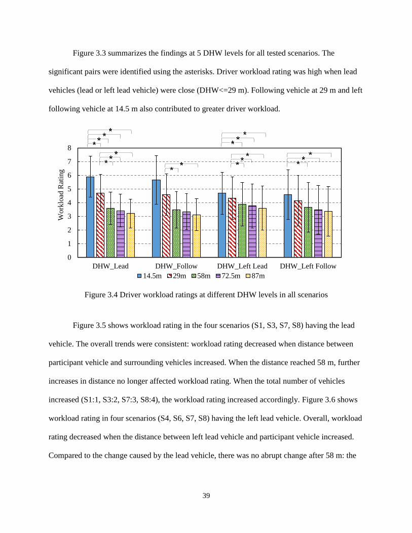
39
Figure 3.3 summarizes the findings at 5 DHW levels for all tested scenarios. The
significant pairs were identified using the asterisks. Driver workload rating was high when lead
vehicles (lead or left lead vehicle) were close (DHW<=29 m). Following vehicle at 29 m and left
following vehicle at 14.5 m also contributed to greater driver workload.
Figure 3.4 Driver workload ratings at different DHW levels in all scenarios
Figure 3.5 shows workload rating in the four scenarios (S1, S3, S7, S8) having the lead
vehicle. The overall trends were consistent: workload rating decreased when distance between
participant vehicle and surrounding vehicles increased. When the distance reached 58 m, further
increases in distance no longer affected workload rating. When the total number of vehicles
increased (S1:1, S3:2, S7:3, S8:4), the workload rating increased accordingly. Figure 3.6 shows
workload rating in four scenarios (S4, S6, S7, S8) having the left lead vehicle. Overall, workload
rating decreased when the distance between left lead vehicle and participant vehicle increased.
Compared to the change caused by the lead vehicle, there was no abrupt change after 58 m: the
0
1
2
3
4
5
6
7
8
DHW_Lead DHW_Follow DHW_Left Lead DHW_Left Follow
Work
load
Rat
ing
14.5m 29m 58m 72.5m 87m

40
decreasing trend was relative smooth. When the total number of vehicles increased (S4:1, S6:2,
S7:3, S8:4), the workload rating increased.
Figure 3.5 Driver workload ratings in four scenarios (S1, S3, S7, S8)
Figure 3.6 Driver workload ratings in four scenarios (S4, S6, S7, S8)
When taking account participants’ speed into the model, the relationship between
subjective rating and continuous variable THW was examined. Table 3.6 shows the regression
0
1
2
3
4
5
6
7
14.5 29 58 72.5 87
Rat
ing
DHW_Lead (m)
S1(1) S3(2) S7(3) S8(4)
0
1
2
3
4
5
6
14.5 29 58 72.5 87
Rat
ing
DHW_LeftLead (m)
S4(1) S6(2) S7(3) S8(4)

41
equations of workload rating based upon inverse THW in each scenario. All the equations used
independent variables have a significant level less than 0.001. No age effect was found.
Table 3.6 Regression equations in different scenarios (Rating)
Scenario Illustration Equation R2
S1 S L
Rating=1.43+1.81/THWLead 0.72
S2 SF
Rating=0.87+0.71/THWFollow 0.58
S3 S LF
Rating=1.68+1.99/THWLead 0.78
S4 S
V1
Rating=1.64+0.74/THWLeftLead 0.50
S5 S
V2
Rating=0.86+0.49/THWLeftFollow 0.66
S6 S
V1V2
Rating=1.95+0.93/THWLeftLead 0.59
S7 S LF
V1
Rating=2.40+1.60/THWLead+0.43/THWLeftLead 0.70
S8 S LF
V1V2
Rating=2.68+1.54/THWLead+0.69/THWLeftLead 0.67
S1-S8 - Rating=1.74+1.74/THWLead+0.20/THWFollow+
0.79/THWLeftLead +0.28/ THWLeftFollow
0.73
3.3.3 Occlusion% (questions 3.2, 3.3)
LMM showed that scenario type was a significant factor on occlusion% (F=23.114,
p=0.000). Post-hoc pairwise comparisons showed that there were significant differences except a
few pairs: scenario 0 and scenario 2/5, scenario 1 and scenario 3/4/6/7/8, scenario 2 and scenario
4/5, scenario 3 and scenario 4/6/7/8, scenario 7 and scenario 8 (Table 3.7). Occlusion% detected
all the no different pairs that rating identified (shown in bold in Table 3.7).

42
The data were then stratified by DHWs. The effect of DHWs on occlusion% in different
scenarios are shown in Table 3.8. When there is a lead vehicle (S1, S3, S7, S8), occlusion% was
sensitive to the DHW of the lead vehicle.
Table 3.7 P values for post-hoc comparisons between all scenario types (occlusion%)
Scenario
type
0
(Mean
=0.347,
SD=0.0
15)
1
(Mean
=0.431,
SD=0.0
09)
2
(Mean
=0.379,
SD=0.0
09)
3
(Mean
=0.428,
SD=0.0
09)
4
(Mean
=0.411,
SD=0.0
09)
5
(Mean
=0.368,
SD=0.0
09)
6
(Mean
=0.421,
SD=0.0
09)
7
(Mean
=0.459,
SD=0.0
04)
8
(Mean
=0.457,
SD=0.0
04)
0 0.000 1.000 0.000 0.013 1.000 0.001 0.000 0.000
1 0.004 1.000 1.000 0.000 1.000 0.265 0.516
2 0.009 0.596 1.000 0.068 0.000 0.000
3 1.000 0.000 1.000 0.116 0.239
4 0.048 1.000 0.000 0.000
5 0.003 0.000 0.000
6 0.009 0.021
7 1.000
8
Table 3.8 The main effects of DHWs on occlusion% in different scenarios
Scenarios Illustration Independent Variables F p
S1 S L
DHWLead 2.615 0.040
S2 SF
DHWFollow 0.970 0.428
S3 S LF
DHWLead 12.338 0.000
S4 S
V1
DHWLeftLead 1.496 0.210
S5 S
V2
DHWLeftFollow 0.423 0.791
S6 S
V1V2
DHWLeftLead 2.135 0.083
S7 S LF
V1
DHWLead 30.317 0.000
DHWLeftLead 2.336 0.054
S8 S LF
V1V2
DHWLead 19.341 0.000
DHWLeftLead 5.46 0.000
S1-S8 - DHWLead 14.949 0.000
DHWFollow 2.501 0.029
DHWLeftLead 9.799 0.000
DHWLeftFollow 1.973 0.080
Note: V1 is the left lead vehicle; V2 is the left following vehicle
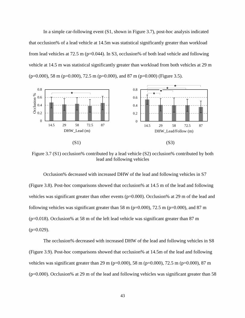
43
In a simple car-following event (S1, shown in Figure 3.7), post-hoc analysis indicated
that occlusion% of a lead vehicle at 14.5m was statistical significantly greater than workload
from lead vehicles at 72.5 m (p=0.044). In S3, occlusion% of both lead vehicle and following
vehicle at 14.5 m was statistical significantly greater than workload from both vehicles at 29 m
(p=0.000), 58 m (p=0.000), 72.5 m (p=0.000), and 87 m (p=0.000) (Figure 3.5).
(S1) (S3)
Figure 3.7 (S1) occlusion% contributed by a lead vehicle (S2) occlusion% contributed by both
lead and following vehicles
Occlusion% decreased with increased DHW of the lead and following vehicles in S7
(Figure 3.8). Post-hoc comparisons showed that occlusion% at 14.5 m of the lead and following
vehicles was significant greater than other events (p=0.000). Occlusion% at 29 m of the lead and
following vehicles was significant greater than 58 m (p=0.000), 72.5 m (p=0.000), and 87 m
(p=0.018). Occlusion% at 58 m of the left lead vehicle was significant greater than 87 m
(p=0.029).
The occlusion% decreased with increased DHW of the lead and following vehicles in S8
(Figure 3.9). Post-hoc comparisons showed that occlusion% at 14.5m of the lead and following
vehicles was significant greater than 29 m (p=0.000), 58 m (p=0.000), 72.5 m (p=0.000), 87 m
(p=0.000). Occlusion% at 29 m of the lead and following vehicles was significant greater than 58
0
0.2
0.4
0.6
0.8
14.5 29 58 72.5 87
Occ
lusi
on %
DHW_Lead (m)
0
0.2
0.4
0.6
0.8
14.5 29 58 72.5 87
DHW_Lead/Follow (m)

44
m (p=0.000). Occlusion% at 14.5 m of the left vehicles was significant greater than 58 m
(p=0.001). Occlusion% at 29 m of the left vehicles was significant greater than 58 m (p=0.003).
Figure 3.8 Occlusion% in S7
Figure 3.9 Occlusion% in S8
Figure 3.10 summarizes the post-hoc findings at all DHW levels in examined scenarios.
DHW of the lead vehicle at 14.5 m resulted in higher occlusion% compared to 29 m (p=0.024)
and 72.5m (p=0.000).
0.3
0.35
0.4
0.45
0.5
0.55
0.6
DHW_Lead=14.5m DHW_Lead=29m DHW_Lead=58m DHW_Lead=72.5m DHW_Lead=87m
Occ
lusi
on %
DHW_LeftLead=14.5 DHW_LeftLead=29 DHW_LeftLead=58
DHW_LeftLead=72.5 DHW_LeftLead=87
0.3
0.35
0.4
0.45
0.5
0.55
0.6
DHW_Lead=14.5m DHW_Lead=29m DHW_Lead=58m DHW_Lead=72.5m DHW_Lead=87m
Occ
lusi
on %
DHW_LeftLead=14.5 DHW_LeftLead=29 DHW_LeftLead=58
DHW_LeftLead=72.5 DHW_LeftLead=87

45
Figure 3.10 Occlusion% at different DHW level in all scenarios
The effect of the DHW of lead vehicle on occlusion% in examined scenarios can be
found in Figure 3.11. When DHW of lead vehicle was 14.5 m, occlusion% was higher than the
rest DHWs.
Figure 3.11 Occlusion% in four scenarios (S1, S3, S7, S8)
When including participants’ speed in the model, the relationship between occlusion%
and continuous variable THW can be found in Table 3.9. Only well predicted regression
equations using backwards elimination are listed (at least one predictor have a significant level
0
0.1
0.2
0.3
0.4
0.5
0.6
0.7
DHW_Lead DHW_Follow DHW_Left Lead DHW_Left Follow
Occ
lusi
on
%
14.5m 29m 58m 72.5m 87m
0.3
0.4
0.4
0.5
0.5
0.6
0.6
14.5 29 58 72.5 87
Occ
lusi
on%
DHW_Lead (m)S1(1) S3(2) S7(3) S8(4)

46
less than 0.05). All the listed independent variables have a significant level of 0.000. No age
effect was found in S7 (0-old; 1-young).
Table 3.9 Regression equations for different scenarios (occlusion%)
Scenario Illustration Equation R2
S3 S LF
Occlusion%=0.34+0.10/THWLead 0.69
Occlusion%=0.30+0.10/THWLead-0.10Age 0.69
S7 S LF
V1
Occlusion%=0.40+0.07/THWLead 0.64
S8 S LF
V1V2
Occlusion%=0.39+0.05/THWLead+0.02/THWLeftLead 0.59
Occlusion%=0.35+0.05/THWLead+0.02/THWLeftLead-0.08Age 0.91
3.3.4 Performance (questions 3.2, 3.3)
The categorization of scenarios indicated that performance statistics were only sensitive
in scenario 8. Thus, the analysis in this section used data from scenario 8. Table 3.10 shows the
effects of DHWs on performance statistics using LMM. Figure 3.12 shows the effect of DHW of
lead vehicle on SDS and the effect of DHW of left lead vehicle on SDSTW.
Table 3.10 the effects of DHWs on performance statistics
Scenarios Dependent
Variables
Independent
Variables
F p
S8
S LF
V1V2
SDS DHWLead 3.176 0.013
DHWLeftLead 0.397 0.812
SDA DHWLead 2.165 0.071
DHWLeftLead 0.574 0.681
SDLP DHWLead 2.285 0.065
DHWLeftLead 0.598 0.677
SDSTW DHWLead 0.781 0.538
DHWLeftLead 2.663 0.032
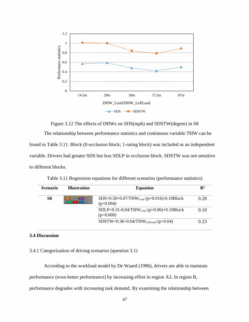
47
Figure 3.12 The effects of DHWs on SDS(mph) and SDSTW(degree) in S8
The relationship between performance statistics and continuous variable THW can be
found in Table 3.11. Block (0-occlusion block; 1-rating block) was included as an independent
variable. Drivers had greater SDS but less SDLP in occlusion block. SDSTW was not sensitive
to different blocks.
Table 3.11 Regression equations for different scenarios (performance statistics)
Scenario Illustration Equation R2
S8
S LF
V1V2
SDS=0.50+0.07/THWLead (p=0.016)-0.10Block
(p=0.004) 0.20
SDLP=0.31-0.04/THWLead (p=0.06)+0.10Block
(p=0.000) 0.10
SDSTW=0.36+0.04/THWLeftLead (p=0.04) 0.23
3.4 Discussion
3.4.1 Categorization of driving scenarios (question 3.1)
According to the workload model by De Waard (1996), drivers are able to maintain
performance (even better performance) by increasing effort in region A3. In region B,
performance degrades with increasing task demand. By examining the relationship between
0
0.2
0.4
0.6
0.8
1
1.2
14.5m 29m 58m 72.5m 87m
Per
form
ace
stat
isti
cs
DHW_Lead/DHW_LeftLead
SDS SDSTW

48
workload rating and performance statistics, scenarios 1, 2, 3, 4, 5, 6, 7 of Experiment 1 were
found to be belong to region A3. Particularly, scenario 7 is at the higher end of region A3 (close
to region B) as the performance improved when workload increased. In scenario 8, SDS
increased when workload increased. Scenario 8 could be categorized in region B and SDS should
be a sensitive workload measure in this study. The results also showed that when workload was
relatively low, drivers were able to maintain lateral position with increased workload. However,
they were not able to drive smoothly in the longitudinal direction (i.e., SDS). This is consistent
with what was found while examining the regression equations for SDS and SDLP: Drivers
tended to compromise speed but still maintain lateral position in occlusion blocks.
3.4.2 Relationship between Distance Headway (DHW) and workload measures (question 3.2)
Using rating as the workload measurement, the main effects of DHWs were found to be
significant in all the scenarios examined. When driving with a lead vehicle (S1 and S3) or a left
lead vehicle (S4 and S6), workload rating at 14.5 m was greater than any other scenarios. While
driving with a following vehicle or a left following vehicle (S2 and S5), workload rating at
14.5 m was greater than events having longer DHWs (58 m, 72.5 m, and 87 m). The workload
rating was affected by the DHWs of vehicles in both lanes (S7 and S8). In both scenarios,
situations where the DHW of lead vehicle at 14.5 m and 29 m should be highlighted as they
contributed to the total workload significantly greater than other levels. While driving with 4
vehicles around (S8), the role of left lead vehicle was reinforced by adding the left following
vehicle. It made the workload ratings with left lead vehicle at 14.5m and 29m greater than any
other events. Thus, 14.5 m was the distance that could contribute to greater workload no matter
which vehicle it was. Besides, when lead vehicle was 58 m or further ahead of the participant’s
vehicle, its DHW no longer affected workload. However, for the left lead vehicle: driver

49
workload always decreased when DHW increased. Generally, in terms of effects of DHWs on
workload in all scenarios, from greatest to least, they were: DHWLead, DHWLeftLead,
DHWLeftFollow, DHWFollow. In addition, with increased number of vehicles, the workload
increased.
Using occlusion as the workload measure, the main effects of DHWs were significant in
S1, S3, S7, and S8, in which there is the lead vehicle. While driving with only following vehicle
(S2) or vehicles in the adjacent lane (S4, S5, and S6), occlusion did not show any significant
differences. In S3, S7, and S8, lead vehicle at 14.5 m resulted in a greater workload compared to
all other events shown by occlusion%. However, in a simple car following event (S1), the
difference between 14.5m and other events was not distinct. Again, the following vehicle
reinforced the role of the lead vehicle.
When examining the performance statistics, SDS was sensitive to changes made by the
lead vehicle whereas SDSTW was sensitive to changes made by the left lead vehicle. Drivers
tended to compromise speed (SDS) but still maintain lateral position (SDLP) when workload
increased.
In summary, workload rating was sensitive to DHW levels of all the vehicles around
while occlusion% was only sensitive to DHW levels in scenarios having a lead vehicle. SDS was
sensitive to the changes made by vehicles in the same lane with participant (i.e., lead vehicles).
SDSTW was sensitive to changes made by vehicles in the adjacent lane (i.e., left lead vehicles).
3.4.3 The Model using Time Headway (THW) to predict workload (question 3.3)
When modeling rating using THWs, the regression equations can be used to describe the
workload rating (Table 3.6). No age effect was found. While modeling occlusion using THWs,
S3, S7, and S8 can be well described using regression equations (Table 3.9). All these three

50
scenarios have a lead vehicle. However, the simple car following event (S1) cannot be described
using THW. In S7, the THW of left lead vehicle was not a significant predictor. The age effect
was found in occlusion measure modeling. If considering age as a predictor, the occlusion
regression equation can count for most of the variances (91%). For scenarios having no lead
vehicle (S2, S4, S5, and S6), the occlusion cannot be modelled using THW. While modeling
performance statistics using THWs, there were some significant predictors (Table 3.11).
However, the R2s were low.
In sum, the workload model works for both rating and occlusion%. However, occlusion%
was not sensitive to scenarios having no lead vehicles and simple car-following event (S1).
Performance statistics were not able to be well predicted using the proposed model.
3.4.4 Differences between workload measures (question 3.4)
While examining the effect of scenario type on workload measures, the occlusion%
statistic identified fewer significantly different pairs than the workload ratings (Table 3.7). Thus,
in terms of identifying the effect of scenario type on workload, occlusion% was less sensitive
compared to rating.
Significant differences were observed in all scenarios using ratings as the workload
measure (Table 3.5). When examining the effect of DHWs on occlusion%, no significant effect
was found in scenarios only having vehicles in the adjacent lane (S4, S5, and S6 in Table 3.8).
Occlusion% was less sensitive to workload contributed by vehicles in the adjacent lane
compared to rating. In addition, the following vehicle had no effect on occlusion% (S2 in Table
3.8). In terms of examining the main effect of DHWs on the most complicated driving scenarios
(i.e., S8), rating and occlusion% were consistent: both DHWs of vehicles in participant’s lane
and adjacent lane had significant effects on total workload (S8 in Table 3.5 and Table 3.8).

51
While modeling the workload rating using inverse THWs, the workload rating was
sensitive to inverse THW in all scenarios. However, occlusion% was less sensitive in the
proposed workload modeling, as only three scenarios having the lead vehicle can be modeled
using inverse THWs. In other words, occlusion% was more sensitive in scenarios where there
was a lead vehicle in front of the participant when workload level was low. However,
occlusion% can be well described using the proposed model (Rocclusion2=0.91, Rrating
2=0.73). The
age effect was not observed while using rating but was observed using occlusion% in S3 and S8.
For future studies, if controlling age effect is desired, anchored rating should be chosen as the
measure for workload.
In sum, though occlusion% was less sensitive to scenarios having no lead vehicles, it can
be well modelled using the proposed workload model. Workload rating was sensitive in all
scenarios and had no age effect.

52
References
Patten, C. J., Kircher, A., Östlund, J., Nilsson, L., & Svenson, O. (2006). Driver experience and
cognitive workload in different traffic environments. Accident Analysis & Prevention, 38(5),
887-894.
Piechulla, W., Mayser, C., Gehrke, H., & König, W. (2003). Reducing drivers’ mental workload
by means of an adaptive man–machine interface. Transportation Research Part F: Traffic
Psychology and Behaviour, 6(4), 233-248.
Taieb-Maimon, M., & Shinar, D. (2001). Minimum and comfortable driving headways: Reality
versus perception. Human Factors, 43(1), 159-172.
Vogel, K. (2002). What characterizes a “free vehicle” in an urban area?. Transportation
Research Part F: Traffic Psychology and Behaviour, 5(1), 15-29.

53
CHAPTER 4
An Experimental Investigation of How Dynamic Traffic Affects Driver Workload
4.1 Introduction
In the previous chapter, static traffic was defined as scenarios when there were no relative
movements among vehicles (fixed headways, same velocity, no lane changes). In this chapter,
dynamic traffic is defined as scenarios when there are relative movements between vehicles
(different velocities, sometimes changing lanes). While experiencing various relative speeds,
participants were asked to drive either in the faster lane or the slower lane. Participants
experienced different lane change urgencies by changing how fast the lane change vehicle turned
its steering wheel.
This driving simulator experiment addresses the following questions:
(4.1) How do the traffic elements (i.e., relative velocity, lane change urgency, drive in the
slower/faster lane, number of vehicles) affect workload measures?
(4.2) How well are workload measures in this study predicted by the workload model
(based upon inverse THW and TTC)?
(4.3) What are the differences among the anchored ratings, occlusion measure, and
performance statistics in dynamic traffic?

54
4.2 Methods
4.2.1 Participants
Twenty-five participants (14 males, and 11 females) were recruited. Eight (3 males and 5
females) of them were elderly participants (age>65) and seventeen (11 males and 6 females) of
them were young participants (21-30 years old). It should be noted that elderly participants were
not able to complete the occlusion task in this experiment because of the high workload of the
driving task (some of them reported that they wanted to press the button very frequently but they
cannot do it due to arthritis). Thus occlusion data was collected only from young participants.
Only experienced drivers were recruited (at least 5-years-experience and driving at least 5000
miles/year). Participants’ far vision was required to be 20/50 or better.
4.2.2 Workload measures and experiment design
The dependent variables were: the anchored rating, occlusion%, and driving performance
statistics (SDS, SDA, SDLP, SDSTW). Independent variables include two sets: categorical set
and continuous set. The categorical set includes relative velocity, lane change urgency, the lane
the driver was in (slower/faster lane), and number of vehicles. The continuous set includes
inverse THW and inverse TTC. Both the categorical set and the continuous set were used to
describe dynamic traffic. The categorical set serves the purpose of providing intuitive feedback
of how people perceive workload in various dynamic scenarios. The continuous set was applied
to show the workload model presented in Chapter 2. In addition, the continuous set could
describe the scenario more comprehensively than categorical set. If any elements change in
dynamic scenarios (even traffic elements that were not included in the categorical set), the
proposed continuous set can always be used to describe the scenario.

55
Table 4.1 shows the number of cases examined in each scenario. D1-D5 are the scenarios
in which participants are in the slower lane while D6-D10 are the scenarios in which participants
are in the faster lane. Relative velocity has 3 levels (7 mph/14 mph/21 mph) and lane change
urgency has 3 levels (none/smooth/sharp). In total, the number of cases examined was 54.
Table 4.1 The number of cases examined in dynamic traffic.
Scenarios Illustration Independent
Variable
Levels No. of cases
examined
D1 S LF
V1+V2+
V’(relative
velocity)
3 3
D2 S LF
V1+V2+ L
V’, ɵ 3x2 6
D3 S LF
V1+V2+
V1+
V’, ɵ 3x2 6
D4 S LF
V1+V2+ L V3+
V4
V’, ɵ 3x2 6
D5 S LF
V1+V2+
V1+
V3+
V4
V’, ɵ 3x2 6
D6 S+ L+F+
V1V2
V’ 3 3
D7 S+ L+F+
V1V2 L+
V’, ɵ 3x2 6
D8 S+ L+F+
V1V2
V1
V’, ɵ 3x2 6
D9 S+ L+F+
V1V2 L V3
V4+
V’, ɵ 3x2 6
D10 S+ L+F+
V1V2
V1
V3
V4+
V’, ɵ 3x2 6
Total 54
Note: V’ = relative velocity; ɵ = lane change urgency
4.2.3 Experiment Setup
A fixed-base mid-fidelity driving simulator running MiniSim v2.0 software was used for
this experiment (http://www.nads-sc.uiowa.edu/minisim/). The simulator consists of a car seat

56
mounted on a motion platform, three HDMI resolution 55-inch monitors forming a 120-degree
field of view, speakers to produce sounds, a simulated instrument panel, a steering wheel and
foot pedals, and software to generate the road scenes and collect the driving performance data
(steering wheel angle, pedal positions, speeds, and the locations as well as characteristics of all
vehicles in the scene). The simulation helped participants drive at the desired speed. If they
drove too slowly, the car following them honked, just as a real car would. If they drove too fast,
then a voice would say “Please slow down”. The occlusion measure was the same as the
previous experiment. The driving scene was blocked unless the driver pressed a button on the
steering wheel. For each button press, the driving scene will be viewable for 0.5s.
4.2.4 Procedure
Participants completed the consent and demographic forms as well as driving history
questionnaires before the experiment. Then, their far acuity was checked to meet the
requirement. Next, each participant learned how to drive the simulator, how to drive and rate the
workload simultaneously, and how to drive while the road scene was intermittently occluded.
Then, participants were instructed to drive 4 test blocks: rating in faster lane, rating in slower
lane, occlusion task in faster lane, occlusion task in slower lane. It took approximately 10
minutes to complete each block. The sequence of the four blocks was arranged within each age
group to counterbalance the learning effect.
In the two anchored rating blocks, participants were asked to answer “what is the current
workload?” during each of the designated driving segments. Anchored clips were presented as a
5 s loops, with both clips appearing simultaneously on a display below the road scene.
Participants were asked to report the highest workload level they experienced within 5s. In the

57
two occlusion test blocks, visual occlusion was collected. In all four blocks, performance data
were recorded at 60 Hz.
4.2.5 Statistical Analysis
LMM was employed to examine the relationship between workload rating and each
performance measure. LMM was also employed to examine the effect of categorical set and
continuous set on workload measures. Participants were modeled as a random effect. The
residual plot was drawn to make sure the data meets linearity and homoskedasticity assumptions.
In all post-hoc analyses, Bonferroni correction was applied. Similar to the previous chapter, there
is no widely accepted R2 for LMM, and the R2 here was calculated based on the definition of
coefficient in the fixed-effects world:
𝑅2 = 1 −∑ (𝑦𝑖 − 𝑦�̂�)
2𝑁𝑖−1
∑ (𝑦𝑖 − 𝑦�̅�)2𝑁𝑖−1
The purpose of providing this number in LMM was to show the proportion of variance
that was explained by the proposed model.
4.3 Results
4.3.1 The effects of traffic elements on anchored rating (question 4.1)
Table 4.2 shows that all the main effects and two-way interaction effects were
statistically significant. Figure 4.1 shows that participants experienced higher workload in the
faster lane compared to the slower lane (p=0.001). Post-hoc test (Figure 4.2) indicates that
participants experienced significant lower workload when the relative velocity was 7 mph
(p7vs14=0.003, p7vs21=0.001) compared to 14/21 mph. Post-hoc test (Figure 4.2) also shows that
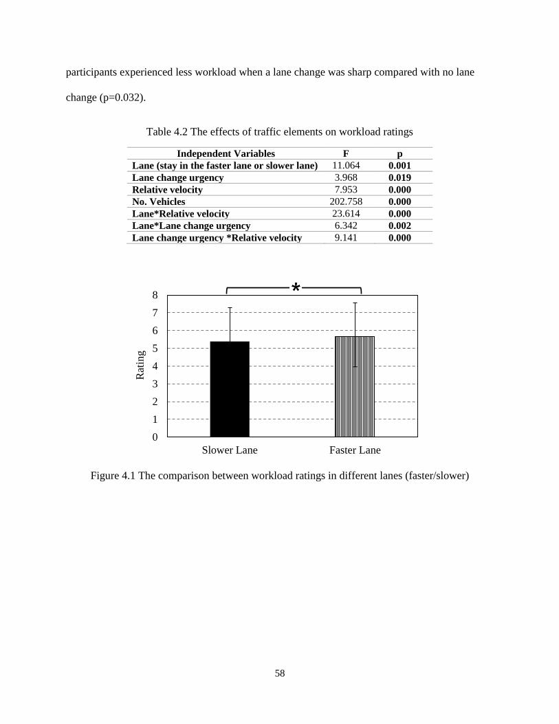
58
participants experienced less workload when a lane change was sharp compared with no lane
change (p=0.032).
Table 4.2 The effects of traffic elements on workload ratings
Independent Variables F p
Lane (stay in the faster lane or slower lane) 11.064 0.001
Lane change urgency 3.968 0.019
Relative velocity 7.953 0.000
No. Vehicles 202.758 0.000
Lane*Relative velocity 23.614 0.000
Lane*Lane change urgency 6.342 0.002
Lane change urgency *Relative velocity 9.141 0.000
Figure 4.1 The comparison between workload ratings in different lanes (faster/slower)
0
1
2
3
4
5
6
7
8
Slower Lane Faster Lane
Rat
ing

59
Figure 4.2 The comparison among workload ratings with different relative velocities
Figure 4.3 The comparison among workload ratings with different lane change actions
Figure 4.4 shows the interaction effect (p=0.000) between lane and relative velocity. In
the slower lane, participants experienced higher workload when the relative velocity between
0
1
2
3
4
5
6
7
8
RelativeV=7 mph RelativeV=14 mph RelativeV=21 mph
Rat
ing
0
1
2
3
4
5
6
7
8
NoLC SmoothLC SharpLC
Rat
ing

60
two lanes was low. In the faster lane, participants experienced lower workload when the relative
velocity between two lanes was low.
Figure 4.4 Interaction effect between relative velocity and lane on ratings
Figure 4.5 shows the interaction effect (p=0.002) between lane and lane change urgency.
When a sharp lane change was presented, participants experienced higher workload while
driving in the slower lane. In contrast, participants experienced greater workload in the faster
lane when a smooth lane change was presented or there was no lane change. When there was a
lane change action, the difference between faster lane and slower lane was no longer obvious.
4.6
4.8
5
5.2
5.4
5.6
5.8
6
6.2
RelativeV=7 mph RelativeV=14 mph RelativeV=21 mph
Rat
ing
Slower Lane Faster Lane

61
Figure 4.5 Interaction effect between lane change urgency and lane on ratings
Figure 4.6 shows the interaction effect (p=0.000) between lane change urgency and
relative velocity. When the relative velocity was low (RelativeV=7 mph), lane change action or a
faster lane change action resulted in higher ratings. In contrast, when the relative velocity
increased (RelativeV=14 mph/21mph), rating was higher when it was a smooth/no lane change
compared to sharp lane changes.
Figure 4.6 Interaction effect between relative velocity and lane change urgency on ratings
4.8
5
5.2
5.4
5.6
5.8
6
6.2
Slower Lane Faster Lane
Rat
ing
NoLC SmoothLC SharpLC
4
4.5
5
5.5
6
6.5
NoLC SmoothLC SharpLC
Rat
ing
RelativeV=7 mph RelativeV=14 mph RelativeV=21 mph

62
4.3.2 The effects of traffic elements on occlusion% (question 4.1)
Table 4.3 shows that all the main effects of traffic elements on occlusion% were
statistically significant. Figure 4.7 shows that participants spent more time looking at the roads in
the faster lane compared to the slower lane (p=0.036). Post-hoc test (Figure 4.8) did not show
any statistical significant pairs among the different relative velocities. However, the comparison
between 7 mph and 21 mph did show engineering significant (p=0.067, using Bonferroni
correction). If no correction was applied, then 14mph (p=0.037) and 21 mph (p=0.022) resulted
in greater occlusion% compared to 7 mph. Post-hoc test (Figure 4.9) also shows that participants
spent more time on looking at the roads when there was no lane change compared to smooth
(p=0.003)/sharp lane change (p=0.001).
Table 4.3 The effects of traffic elements on occlusion%
Independent Variables F p
Lane (stay in faster lane or not) 4.418 0.036
Lane change urgency 6.399 0.002
Relative velocity 3.204 0.041
No. Vehicles 4.401 0.036
Lane*Relative velocity 18.781 0.000
Lane*Lane change urgency 1.272 0.281
Lane change urgency*Relative velocity 4.930 0.001

63
Figure 4.7 The comparison between occlusion% in different lanes (faster/slower)
Figure 4.8 The comparison among occlusion% with different relative velocities.
0%
10%
20%
30%
40%
50%
60%
70%
Slower Lane Faster Lane
Occ
lusi
on
%
0%
10%
20%
30%
40%
50%
60%
70%
RelativeV=7 mph RelativeV=14 mph RelativeV=21 mph
Occ
lusi
on%

64
Figure 4.9 The comparison among occlusion% with different lane change events
Figure 4.10 shows, in the slower lane, participants spent more time on looking at roads
when the relative velocity is low. In the faster lane, participants spent less time looking when the
relative velocity is low (p=0.000).
Figure 4.10 Interaction effect between relative velocity and lane on occlusion%
0%
10%
20%
30%
40%
50%
60%
70%
NoLC SmoothLC SharpLC
Occ
lusi
on%
34%
36%
38%
40%
42%
44%
46%
48%
RelativeV=7 mph RelativeV=14 mph RelativeV=21 mph
Occ
lusi
on%
Slower Lane Faster Lane
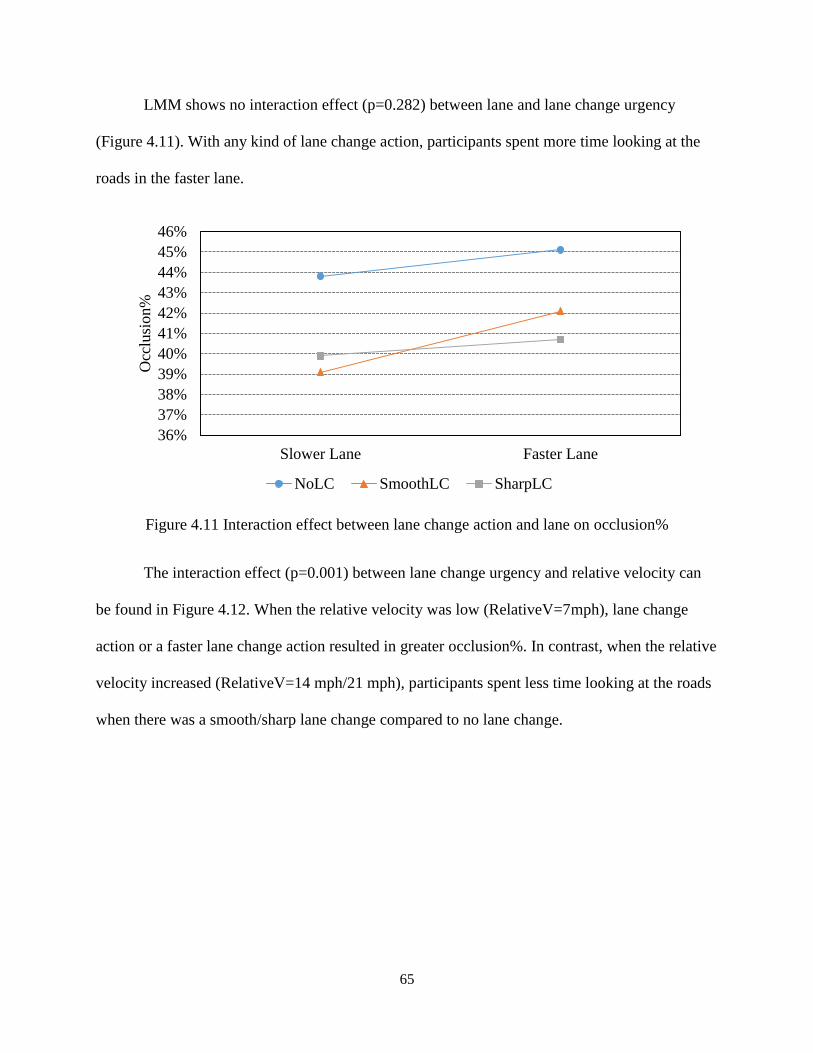
65
LMM shows no interaction effect (p=0.282) between lane and lane change urgency
(Figure 4.11). With any kind of lane change action, participants spent more time looking at the
roads in the faster lane.
Figure 4.11 Interaction effect between lane change action and lane on occlusion%
The interaction effect (p=0.001) between lane change urgency and relative velocity can
be found in Figure 4.12. When the relative velocity was low (RelativeV=7mph), lane change
action or a faster lane change action resulted in greater occlusion%. In contrast, when the relative
velocity increased (RelativeV=14 mph/21 mph), participants spent less time looking at the roads
when there was a smooth/sharp lane change compared to no lane change.
36%
37%
38%
39%
40%
41%
42%
43%
44%
45%
46%
Slower Lane Faster Lane
Occ
lusi
on
%
NoLC SmoothLC SharpLC

66
Figure 4.12 Interaction effect between relative velocity and lane change urgency on occlusion%
4.3.3 The effects of traffic elements on performance (question 4.1)
Table 4.4 shows that performance statistics were positively correlated with anchored
rating. In other words, higher workload is associated with poorer performance (larger SD). The
task demands of all the tested dynamic scenarios should fall in region B in De Waard model. It
indicated that the performance measures should be sensitive to workload in dynamic traffic. In
the first experiment (Chapter 3), only some of the performance statistics showed its correlation
with rating in the most complicated static traffic scenario (S8) (Table 3.3).
20%
25%
30%
35%
40%
45%
50%
55%
60%
NoLC SmoothLC SharpLC
Occ
lusi
on%
RelativeV=7 mph RelativeV=14 mph RelativeV=21 mph

67
Table 4.4 The relationship between performance statistics and anchored rating
Performance Statistics p value
SDS 0.000 (+)
SDA 0.000 (+)
SDLP 0.000 (+)
SDSTW 0.000 (+)
Note: plus signs show DV and IDV are positively correlated.
Then how traffic elements affect each of the performance statistics is in Table 4.5. No
age effect was found in analyzing any of the performance statistics.
Table 4.5 The effects of traffic elements on performance statistics
Dep. Variables Independent Variables F p
SDS
Lane 0.000 0.995
Lane change urgency 2.382 0.093
Relative velocity 3.765 0.023
No. Vehicles 1.152 0.283
Lane *Lane change urgency 1.088 0.337
Lane *Relative velocity 7.643 0.001
Lane change urgency*Relative velocity 1.368 0.243
SDA
Lane 21.060 0.000
Lane change urgency 6.131 0.002
Relative velocity 10.657 0.000
No. Vehicles 0.371 0.543
Lane *Lane change urgency 1.536 0.216
Lane *Relative velocity 6.455 0.002
Lane change urgency*Relative velocity 1.151 0.331
SDLP
Lane 3.260 0.071
Lane change urgency 9.756 0.000
Relative velocity 6.219 0.002
No. Vehicles 1.061 0.303
Lane *Lane change urgency 5.929 0.003
Lane *Relative velocity 1.639 0.195
Lane change urgency*Relative velocity 1.859 0.115
SDSTW
Lane 0.411 0.521
Lane change urgency 4.720 0.009
Relative velocity 4.751 0.009
No. Vehicles 0.106 0.745
Lane *Lane change urgency 3.976 0.019
Lane *Relative velocity 4.931 0.007
Lane change urgency*Relative velocity 0.564 0.688

68
Figure 4.13 shows the main effects of lane on performance statistics. Figure 4.14 shows
the main effects of lane change urgency on performance statistics. Figure 4.15 shows the main
effects of relative velocity on performance statistics. The significant pairs were indicated using
the asterisks. The interaction effect of lane and relative velocity for all four performance
statistics are shown in Figure 4.16. The interaction effect of lane and lane change urgency for
SDLP and SDSTW can be found in Figure 4.17.
Figure 4.13 The main effects of block on performance statistics
0
0.2
0.4
0.6
0.8
1
1.2
SDS(mph) SDA(ft/S2) SDLP(ft) SDSTW(degree)
Per
form
ance
sta
tist
ics
Slower Lane Faster Lane

69
Figure 4.14 The main effects of lane change urgency on performance statistics
Figure 4.15 The main effects of relative velocity on performance statistics
0
0.2
0.4
0.6
0.8
1
1.2
1.4
SDS(mph) SDA(ft/S2) SDLP(ft) SDSTW(degree)
Per
form
ance
sta
tist
ics
NoLC SmoothLC SharpLC
0
0.2
0.4
0.6
0.8
1
1.2
1.4
SDS(mph) SDA(ft/S2) SDLP(ft) SDSTW(degree)
Per
form
ance
sta
tist
ics
7 mph 14 mph 21 mph

70
Figure 4.16 The interaction effect of relative velocity and lane on performance statistics
Figure 4.17 The interaction effect of lane change action and lane on some performance statistics
4.3.4 The effects of continuous set on workload measures (question 4.2)
To evaluate the proposed workload model, the traffic elements should be described
quantitatively in a universal way using inverse THW and TTC. Table 4.6 shows predicted
0.6
0.7
0.8
0.9
1
1.1
1.2
1.3
7 mph 14 mph 21 mph
SD
S (
mp
h)
Slower Lane Faster Lane
0
0.2
0.4
0.6
0.8
1
7 mph 14 mph 21 mph
SD
A (
ft/S
2)
Slower Lane Faster Lane
0.2
0.22
0.24
0.26
0.28
0.3
0.32
0.34
0.36
7 mph 14 mph 21 mph
SD
LP
(fe
et)
Slower Lane Faster Lane
0.3
0.35
0.4
0.45
0.5
0.55
7 mph 14 mph 21 mph
SD
ST
W (
deg
ree)
Slower Lane Faster Lane
0.2
0.25
0.3
0.35
0.4
NoLC SmoothLC SharpLC
SD
LP
(fe
et)
Slower Lane Faster Lane
0.3
0.35
0.4
0.45
0.5
0.55
NoLC SmoothLC SharpLC
SD
ST
W (
deg
ree)
Slower Lane Faster Lane
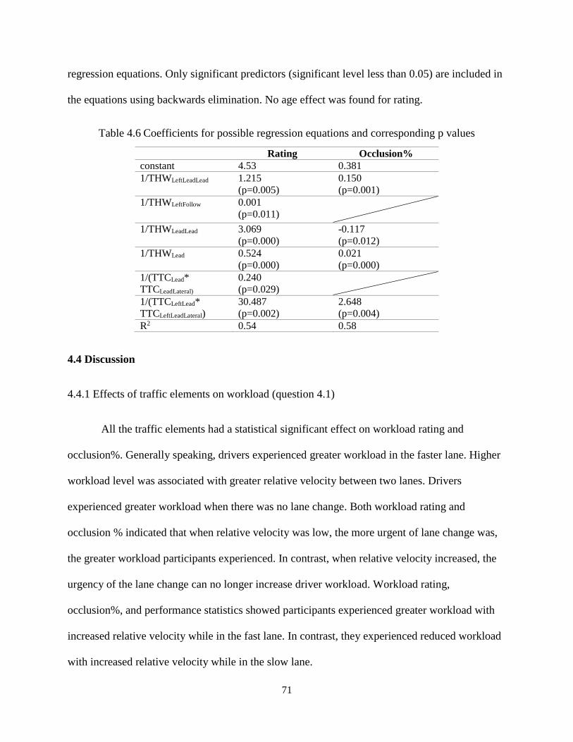
71
regression equations. Only significant predictors (significant level less than 0.05) are included in
the equations using backwards elimination. No age effect was found for rating.
Table 4.6 Coefficients for possible regression equations and corresponding p values
Rating Occlusion%
constant 4.53 0.381
1/THWLeftLeadLead 1.215
(p=0.005)
0.150
(p=0.001)
1/THWLeftFollow 0.001
(p=0.011)
1/THWLeadLead 3.069
(p=0.000)
-0.117
(p=0.012)
1/THWLead 0.524
(p=0.000)
0.021
(p=0.000)
1/(TTCLead*
TTCLeadLateral)
0.240
(p=0.029)
1/(TTCLeftLead*
TTCLeftLeadLateral)
30.487
(p=0.002)
2.648
(p=0.004)
R2 0.54 0.58
4.4 Discussion
4.4.1 Effects of traffic elements on workload (question 4.1)
All the traffic elements had a statistical significant effect on workload rating and
occlusion%. Generally speaking, drivers experienced greater workload in the faster lane. Higher
workload level was associated with greater relative velocity between two lanes. Drivers
experienced greater workload when there was no lane change. Both workload rating and
occlusion % indicated that when relative velocity was low, the more urgent of lane change was,
the greater workload participants experienced. In contrast, when relative velocity increased, the
urgency of the lane change can no longer increase driver workload. Workload rating,
occlusion%, and performance statistics showed participants experienced greater workload with
increased relative velocity while in the fast lane. In contrast, they experienced reduced workload
with increased relative velocity while in the slow lane.

72
The effects of traffic elements on performance statistics varied. Only SDA identified the
main effect of lane on workload. Only lateral statistics (i.e., SDLP, SDSTW) were able to
identify the main effect of lane change urgency. All the performance statistics identified the main
effects of relative velocity.
4.4.2 Workload model determined by THW and Time to Collision (TTC) (question 4.2)
Both rating and occlusion% can be described using the proposed model. The regression
equations showed the relative importance of each component. However, the R2 was less than
desired for rating. One possible source of noise could come from the way that participants
considered lane change actions in terms of its effect on total workload. Lane changes were not
shown in the anchored clips.
Two less term was included in modeling occlusion%: it was not sensitive to the left
following vehicle (same characteristic while examining it in static traffic). When the lead lead
vehicle was too close, the occlusion% dropped. This can be explained by the trade-off between
performance and workload level: When there were too many activities happening in the scene,
participants can no longer fully involved in the driving task. Thus, the occlusion% decreased. It
shows that occlusion% is no longer a sensitive measure when workload level is high.
4.4.3 Differences among workload measures (question 4.3)
In terms of how traffic elements affect rating/occlusion%, the interaction between lane
and lane change urgency was not consistent. When there was a sharp lane change, drivers
experienced higher workload level in slower lane measured by rating. However, occlusion% was
not able to detect the interaction effect: at different lane change urgency levels, participants
experienced higher workload while driving in the faster lane compared to the slower lane.

73
While examining the main effect of lane change urgency, rating showed higher workload
was associated with no lane change and participants spent shorter time observing the road when
there was a sharp lane change activity. In addition, analyses showed the main effect of lane
change urgency on performance statistics was significant: greater longitudinal statistic (i.e.,
SDA) were associated with no lane change events; smaller lateral measures were associated with
no lane change events. Two conclusions can be drawn here: (1) rating, occlusion%, and
longitudinal measures are consistent in terms of capturing workload level in different levels of
lane change urgency; However, (2) What actually captured was the trade-off between workload
level and performance: when there was a lane change action, lateral performance decreased; at
the same time, participants were not able to actively be involved in rating/occlusion task/velocity
maintaining task as the most critical task for them was stay in the right lane. Thus, all these
measures dropped. As mentioned in the previous chapter, occlusion% was sensitive in scenarios
where there was a lead vehicle in front of the participant when workload level was low. In high
workload scenarios contributed by lane change activities, occlusion% cannot reflect actual
workload level.
Here is a summary of all the workload measures examined in the dissertation:
(1) Anchored ratings are a sensitive workload measure and they are unaffected by age.
(2) Occlusion measure is a sensitive measure of workload, when the workload level is
low. At high levels of workload, the act of pressing the button is a sufficiently loading task that it
interferes with driving, and therefore occlusion% becomes a less accurate indicator of workload.
(3) Performance statistics were influenced by driving, which indicated that drivers paid
more attention to the lane keeping task than velocity control in the tested scenarios. In future

74
workload studies, besides the verification of the sensitivity of performance measure, multiple
performance statistics should be applied as one performance measure cannot illustrate the full
story of how participants drive.

75
CHAPTER 5
GOMS Modeling of Driver Workload in Static and Dynamic Traffic
5.1 Introduction
In this chapter, GOMS model (Card et al., 1983) is used to model driver workload.
GOMS represents Goals, Operators, Methods, and Selection rules. It is a method that uses
production rules. The GOMS model is widely used to predict learning time and performance
time of procedural tasks.
There are several GOMS family models. The simplest one is the Keystroke-Level Model
(KLM, Card et al., 1980), which can be used to predict the total execution time for elementary
keystroke actions. The most complex one is Cognitive Perceptual Motor GOMS (CPM-GOMS,
Gray et al., 1993), which predicts execution time using a schedule chart mapped out by motor
processes. Natural GOMS Language (NGOMSL, Keiras, 1997) is a method in between these two
methods: structured natural language is used to describe the procedural knowledge that a user
must follow to get the task done. A NGOMSL model decomposes the main goal into several sub-
goals. All the sub-goals can be described at the level of basic operators.
As mentioned above, GOMS models were primarily used to predict time. No previous
research used GOMS model only to predict workload. To model workload in this chapter, a time
line model is used. Mental workload can be described as “the relation between the function
relating the mental resources demanded by a task and those resources available to be supplied by

76
the human operator” (Parasuraman et al., 2008). The time line model (North and Riley, 1989)
satisfies the definition by using timerequired to represent mental resources demanded and
timeavailable representing mental resources available. Thus, it is proposed that the use of expected
workload (Equation 5.1) is an index of workload.
ExpectedWorkload = 𝑇𝑖𝑚𝑒𝑟𝑒𝑞𝑢𝑖𝑟𝑒𝑑
𝑇𝑖𝑚𝑒𝑎𝑣𝑎𝑖𝑙𝑎𝑏𝑙𝑒 (5.1)
5.2 Methods
To model driver workload using NGOMSL, a task analysis was conducted in the format
of a flow chart (Figure 5.1). Procedure-based task descriptions can be found in Figure 5.2 and
Figure 5.3.
As GOMS models are not designed for concurrent tasks or interferential tasks, in this
research, the “rate workload while driving” is described as one single task: rate workload.
However, the driving task can be embedded into the procedural knowledge that the participant
must follow to get the task done. In this research, the driving task was extracted as looking at the
front view and two other mirrors (i.e., the center mirror and the left side mirror) before each
workload rating. For all driving tasks, it is essential to look at the front view. In addition,
participants were instructed to look at the other two mirrors. Thus, the procedural knowledge
listed did show rules that a participant was supposed to executed.
In the modeling, each step in the GOMSL model takes 50ms to execute. No extra time
was added to total execution time if it’s a primitive mental operator (No long term memory was
involved in the task). In addition, each analyst-defined mental operator (i.e., retain, calculate,
perceive, consider) requires extra 1200ms.
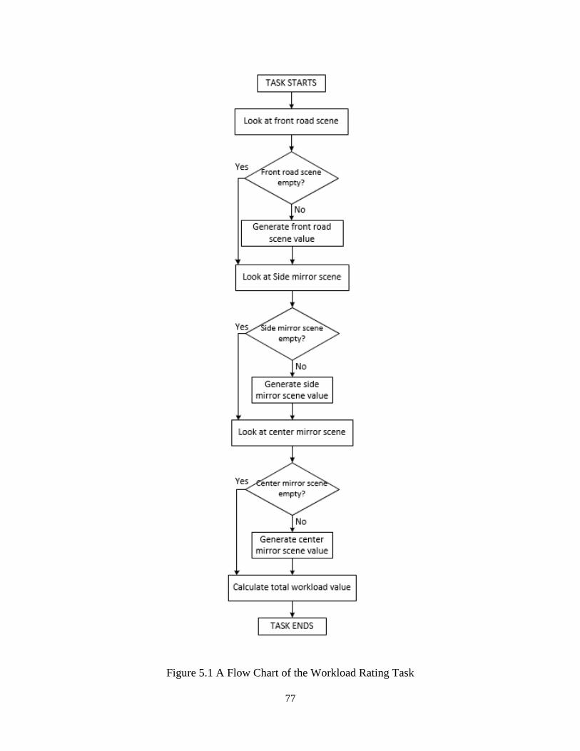
77
Figure 5.1 A Flow Chart of the Workload Rating Task

78
Method for GOAL: Rate Workload while Driving
Step1. Look at <front road scene>
Step2. Accomplish goal: generate workload value of front road scene
Step3. Look at <side mirror scene>
Step4. Accomplish goal: generate workload value of side mirror scene
Step5. Look at <center mirror scene>
Step6. Accomplish goal: generate workload value of center mirror scene
Step7. Accomplish goal: calculate total workload value
Step8. Retrieve <total workload value> from short-term memory
Step9. Report <total workload value>
Step10. Return with goal accomplished
Method for Goal: generate workload level of front road scene
Step1. Decide: If <front road scene> is empty, <front road scene value> = 0 and go to
step 3, else go to step 2.
Step2. Accomplish goal: think about the front road scene value
Step3. Store <front road scene value> to short-term memory
Step4. Return with goal accomplished
Method for Goal: think about the front road scene value
Step1. Compare <front road scene> to < scene of anchor 2>: If <front road scene> is
less busy than <scene of anchor 2>, go to step3, else go to step 2
Step2. Compare <front road scene> to < scene of anchor 6>
Step3. Retain <front road scene value>
Step4. Return with goal accomplished
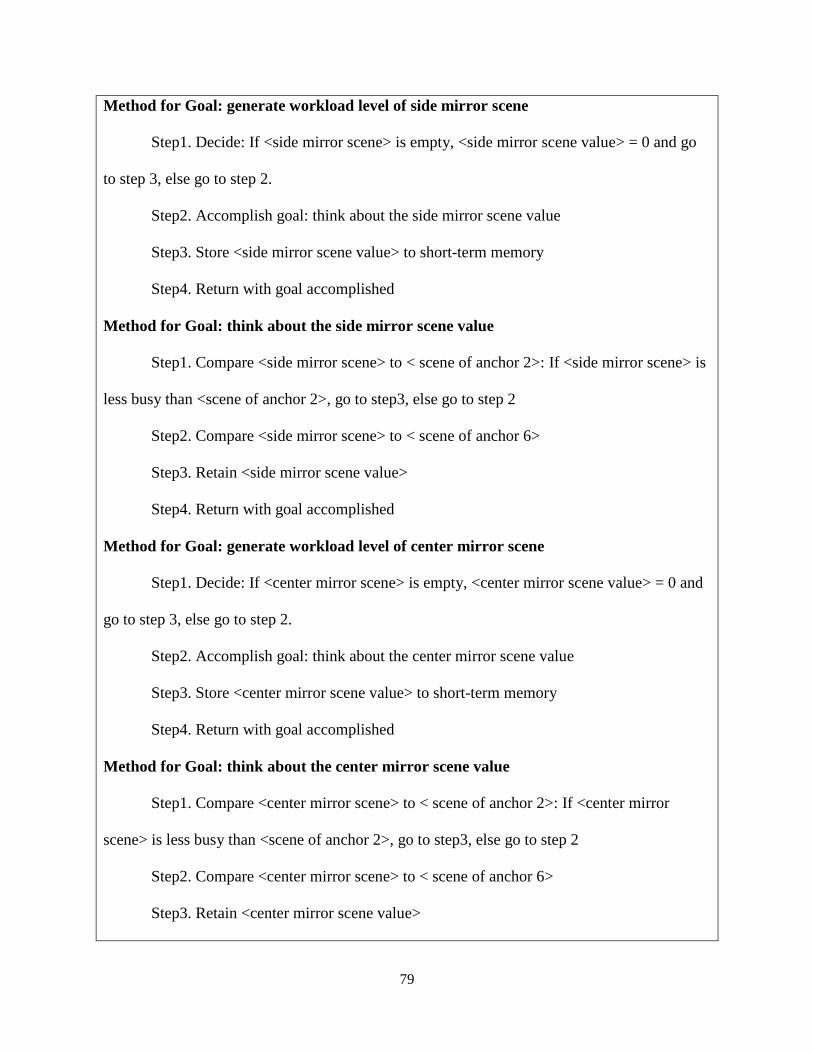
79
Method for Goal: generate workload level of side mirror scene
Step1. Decide: If <side mirror scene> is empty, <side mirror scene value> = 0 and go
to step 3, else go to step 2.
Step2. Accomplish goal: think about the side mirror scene value
Step3. Store <side mirror scene value> to short-term memory
Step4. Return with goal accomplished
Method for Goal: think about the side mirror scene value
Step1. Compare <side mirror scene> to < scene of anchor 2>: If <side mirror scene> is
less busy than <scene of anchor 2>, go to step3, else go to step 2
Step2. Compare <side mirror scene> to < scene of anchor 6>
Step3. Retain <side mirror scene value>
Step4. Return with goal accomplished
Method for Goal: generate workload level of center mirror scene
Step1. Decide: If <center mirror scene> is empty, <center mirror scene value> = 0 and
go to step 3, else go to step 2.
Step2. Accomplish goal: think about the center mirror scene value
Step3. Store <center mirror scene value> to short-term memory
Step4. Return with goal accomplished
Method for Goal: think about the center mirror scene value
Step1. Compare <center mirror scene> to < scene of anchor 2>: If <center mirror
scene> is less busy than <scene of anchor 2>, go to step3, else go to step 2
Step2. Compare <center mirror scene> to < scene of anchor 6>
Step3. Retain <center mirror scene value>

80
Step4. Return with goal accomplished
Method for Goal: Calculate total workload value
Step1. Retrieve <front road scene value> <side mirror scene value> < center mirror
scene value> from short-term memory
Step2. Decide: If <front road scene value> = 0, then go to step 5, else go to step 3
Step3. Calculate <weighted front road scene value>
Step4. Store <weighted front road scene value> to short-term memory
Step5. Decide: If <side mirror scene value> = 0, then go to step 8, else go to step 6
Step6. Calculate <weighted side mirror scene value>
Step7. Store <weighted side mirror scene value> to short-term memory
Step8. Decide: If <center mirror scene value> = 0, then go to step 11, else go to step 9
Step9. Calculate <weighted center mirror scene value>
Step10. Store <weighted center mirror scene value> to short-term memory
Step11. Calculate <total workload value>
Step12. Store <total workload value> to short-term memory
Step13. Return with goal accomplished
Figure 5.2 NGOMSL-Style Description of the Workload Rating Task in Static Traffic
Method for GOAL: Rate Workload while Driving
Step1. Accomplish goal: Look at <front road scene>
Step2. Accomplish goal: generate workload value of front road scene
Step3. Accomplish goal: Look at <side mirror scene>
Step4. Accomplish goal: generate workload value of side mirror scene
Step5. Accomplish goal: Look at <center mirror scene>

81
Step6. Accomplish goal: generate workload value of center mirror scene
Step7. Accomplish goal: calculate total workload value
Step8. Retrieve <total workload value> from short-term memory
Step9. Report <total workload value>
Step10. Return with goal accomplished
Method for Goal: Look at <front road scene>
Step1. Perceive in which lane (slow/fast) the driver is driving
Step2. Store <lane value> to short-term memory
Step3. Perceive the relative velocity (low/medium/high) between two lanes
Step4. Store <relative velocity value> to short-term memory
Step5. Perceive if there is a lane change action.
Step6. Decide: If there is a lane change action, go to Step 7; if no, <lane change
urgency> = 0 and go to Step8.
Step7. Perceive how urgent (smooth/sharp) the lane change action is.
Step8. Store <lane change urgency> to short-term memory.
Step9. Return with goal accomplished
Method for Goal: generate workload level of front road scene
Step1. Compare <front road scene> to < scene of anchor 2>: If <front road scene> is
less busy than <scene of anchor 2>, go to step17, else go to step 2
Step2. Compare <front road scene> to < scene of anchor 6>: If <front road scene> is
less busy than <scene of anchor 6>, go to step17, else go to step 3
Step3. Retrieve <relative velocity value>
Step4. Compare <relative velocity value> to < relative velocity in scene of anchor 6>
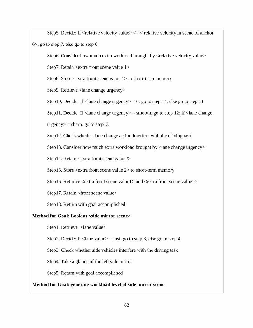
82
Step5. Decide: If <relative velocity value> <= < relative velocity in scene of anchor
6>, go to step 7, else go to step 6
Step6. Consider how much extra workload brought by <relative velocity value>
Step7. Retain <extra front scene value 1>
Step8. Store <extra front scene value 1> to short-term memory
Step9. Retrieve <lane change urgency>
Step10. Decide: If <lane change urgency> = 0, go to step 14, else go to step 11
Step11. Decide: If <lane change urgency> = smooth, go to step 12; if <lane change
urgency> = sharp, go to step13
Step12. Check whether lane change action interfere with the driving task
Step13. Consider how much extra workload brought by <lane change urgency>
Step14. Retain <extra front scene value2>
Step15. Store <extra front scene value 2> to short-term memory
Step16. Retrieve <extra front scene value1> and <extra front scene value2>
Step17. Retain <front scene value>
Step18. Return with goal accomplished
Method for Goal: Look at <side mirror scene>
Step1. Retrieve <lane value>
Step2. Decide: If <lane value> = fast, go to step 3, else go to step 4
Step3: Check whether side vehicles interfere with the driving task
Step4. Take a glance of the left side mirror
Step5. Return with goal accomplished
Method for Goal: generate workload level of side mirror scene
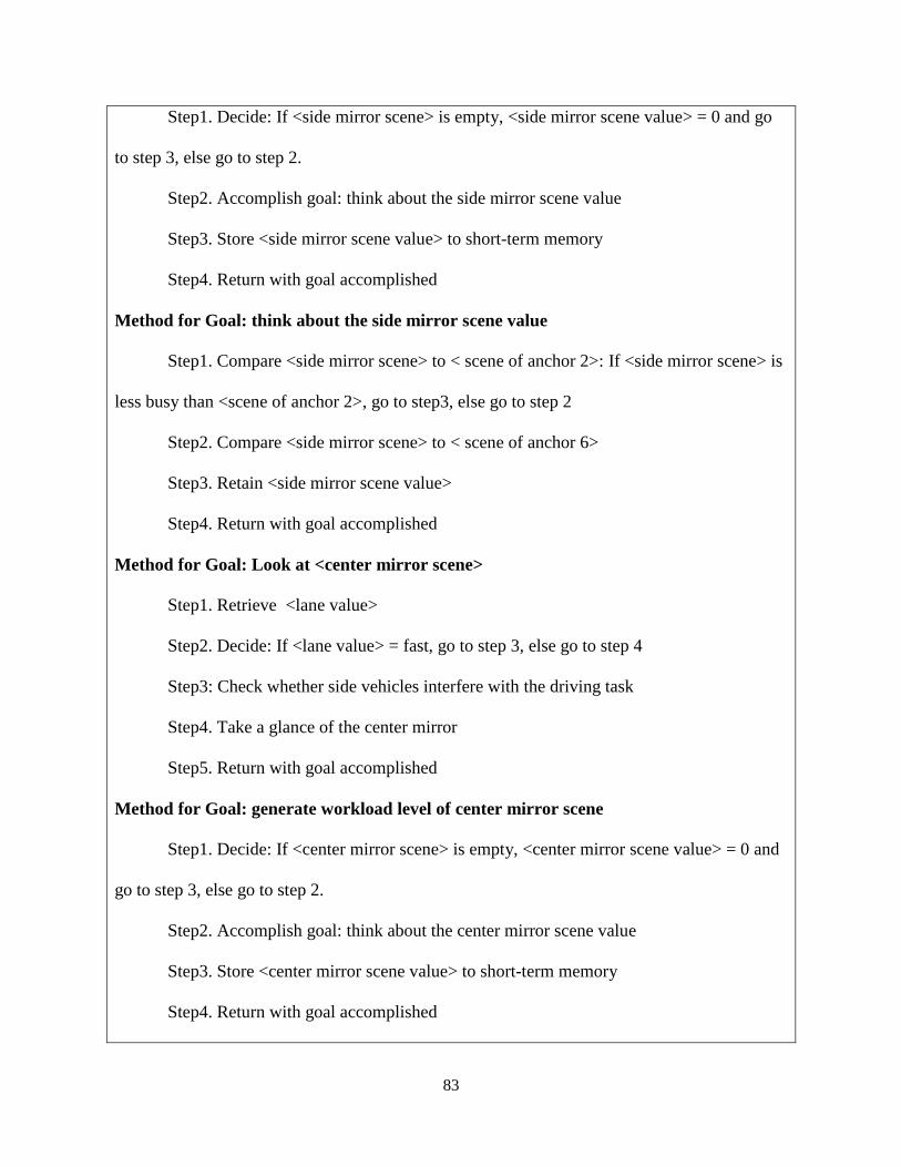
83
Step1. Decide: If <side mirror scene> is empty, <side mirror scene value> = 0 and go
to step 3, else go to step 2.
Step2. Accomplish goal: think about the side mirror scene value
Step3. Store <side mirror scene value> to short-term memory
Step4. Return with goal accomplished
Method for Goal: think about the side mirror scene value
Step1. Compare <side mirror scene> to < scene of anchor 2>: If <side mirror scene> is
less busy than <scene of anchor 2>, go to step3, else go to step 2
Step2. Compare <side mirror scene> to < scene of anchor 6>
Step3. Retain <side mirror scene value>
Step4. Return with goal accomplished
Method for Goal: Look at <center mirror scene>
Step1. Retrieve <lane value>
Step2. Decide: If <lane value> = fast, go to step 3, else go to step 4
Step3: Check whether side vehicles interfere with the driving task
Step4. Take a glance of the center mirror
Step5. Return with goal accomplished
Method for Goal: generate workload level of center mirror scene
Step1. Decide: If <center mirror scene> is empty, <center mirror scene value> = 0 and
go to step 3, else go to step 2.
Step2. Accomplish goal: think about the center mirror scene value
Step3. Store <center mirror scene value> to short-term memory
Step4. Return with goal accomplished

84
Method for Goal: think about the center mirror scene value
Step1. Compare <center mirror scene> to < scene of anchor 2>: If <center mirror
scene> is less busy than <scene of anchor 2>, go to step3, else go to step 2
Step2. Compare <center mirror scene> to < scene of anchor 6>
Step3. Retain <center mirror scene value>
Step4. Return with goal accomplished
Method for Goal: Calculate total workload value
Step1. Retrieve <front road scene value> <side mirror scene value> <center mirror
scene value> from short-term memory
Step2. Calculate <weighted front road scene value>
Step3. Store <weighted front road scene value> to short-term memory
Step4. Decide: If <side mirror scene value> = 0, then go to step 6, else go to step 5
Step5. Calculate <weighted side mirror scene value>
Step6. Store <weighted side mirror scene value> to short-term memory
Step7. Decide: If <center mirror scene value> = 0, then go to step 9, else go to step 8
Step8. Calculate <weighted center mirror scene value>
Step9. Store <weighted center mirror scene value> to short-term memory
Step10. Calculate <total workload value>
Step11. Store <total workload value> to short-term memory
Step12. Return with goal accomplished
Figure 5.3 NGOMSL-Style Description of the Workload Rating Task in Dynamic Traffic
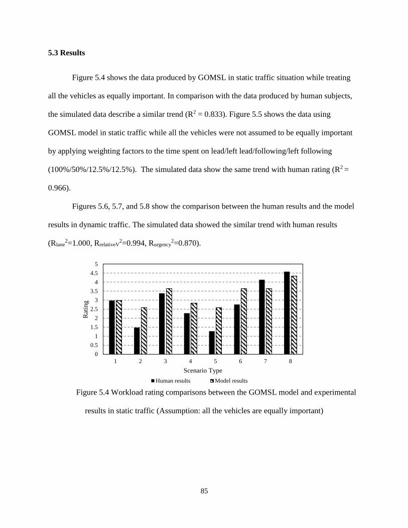
85
5.3 Results
Figure 5.4 shows the data produced by GOMSL in static traffic situation while treating
all the vehicles as equally important. In comparison with the data produced by human subjects,
the simulated data describe a similar trend (R2 = 0.833). Figure 5.5 shows the data using
GOMSL model in static traffic while all the vehicles were not assumed to be equally important
by applying weighting factors to the time spent on lead/left lead/following/left following
(100%/50%/12.5%/12.5%). The simulated data show the same trend with human rating (R2 =
0.966).
Figures 5.6, 5.7, and 5.8 show the comparison between the human results and the model
results in dynamic traffic. The simulated data showed the similar trend with human results
(Rlane2=1.000, RrelativeV
2=0.994, Rurgency2=0.870).
Figure 5.4 Workload rating comparisons between the GOMSL model and experimental
results in static traffic (Assumption: all the vehicles are equally important)
0
0.5
1
1.5
2
2.5
3
3.5
4
4.5
5
1 2 3 4 5 6 7 8
Rat
ing
Scenario Type
Human results Model results
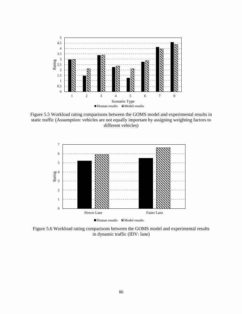
86
Figure 5.5 Workload rating comparisons between the GOMS model and experimental results in
static traffic (Assumption: vehicles are not equally important by assigning weighting factors to
different vehicles)
Figure 5.6 Workload rating comparisons between the GOMS model and experimental results
in dynamic traffic (IDV: lane)
0
0.5
1
1.5
2
2.5
3
3.5
4
4.5
5
1 2 3 4 5 6 7 8
Rat
ing
Scenario Type
Human results Model results
0
1
2
3
4
5
6
7
Slower Lane Faster Lane
Rat
ing
Human results Model results

87
Figure 5. 7 Workload rating comparisons between the GOMS model and experimental results in
dynamic traffic (IDV: relative velocity)
Figure 5. 8 Workload rating comparisons between the GOMS model and experimental results in
dynamic traffic (IDV: the urgency of lane change action)
5.4 Discussion
Using the NGOMSL model, the model simulation was able to generate workload data
that were similar to the human experimental study. However, it should not be expected that
0
1
2
3
4
5
6
7
RelativeV=7MPH RelativeV=14MPH RelativeV=21MPH
Rat
ing
Human results Model results
0
1
2
3
4
5
6
7
No LC Smooth LC Fast LC
Rat
ing
Human results Model results

88
NGOMSL model can produce extremely precise data. In the future, GOMS task analysis can be
used to help experiment design and get an estimation about the possible experimental data.
However, the NGOMSL model was not able to produce data for all the existing
independent variables. In this dissertation, THW and TTC cannot be included in the NGOMSL
model directly, as time variables themselves can hardly be incorporated into procedural
knowledge of the workload rating task. Instead, variables directly manipulated (e.g., number of
vehicles in static traffic, lane change urgency in dynamic traffic) in the design of experiment
were examined using the NGOMSL model.

89
References
Card, S., Moran, T. & Newell, A. (1983). The Psychology of Human-Computer Interaction.
Hillsdale, New Jersey: Erlbaum.
Card, S.K., Moran, T.P., & Newell, A. (1980). The keystroke-level model for user performance
time with interactive systems. Communications of the ACM, 23(7), 396-410.
Gray, W. D., John, B. E., & Atwood, M. E. (1993). Project Ernestine: A validation of GOMS for
prediction and explanation of real-world task performance. Human-Computer Interaction, 8(3),
237-209.
Kieras, D. E. (1997). A Guide to GOMS model usability evaluation using NGOMSL. In M.
Helander,T. Landauer, and P. Prabhu (Eds.), Handbook of Human-Computer Interaction.
(Second Edition). Amsterdam: North-Holland. 733-766.
North, R. A., & Riley, V. A. (1989). W/INDEX: A predictive model of operator workload. In
Applications of Human Performance Models to System Design, 81-89, Springer, Boston, MA.
Parasuraman, R., Sheridan, T. B., & Wickens, C. D. (2008). Situation awareness, mental
workload, and trust in automation: Viable, empirically supported cognitive engineering
constructs. Journal of Cognitive Engineering and Decision Making, 2(2), 140-160.

90
CHAPTER 6
Conclusions
6.1 Dissertation Summary
Minimizing driver errors should improve driving safety. Driver errors are more common
when workload is high than when it is low. Thus, it is of great importance to study workload.
Quantifying driver workload as a function of traffic would benefit driving safety by providing
adequate take-over time, refining adaptive in-vehicle systems, and regulating in-vehicle
secondary tasks.
Among all the factors that affected driver workload, traffic is the one that has not been
systematically varied and examined. Previous research studied qualitatively periodic traffic
instead of quantitatively real-time traffic. In this dissertation, a model relating quantified traffic
to real-time driver workload was investigated and validated. Generally, the driving scenarios
were categorized into static (no relative movements among vehicles) and dynamic (movements
including relative velocity and lane changes). In static scenarios, workload was assumed to be
proportional to inverse THW (TTC is infinity as no relative movements). In dynamic scenarios,
workload was assumed to be proportional to inverse THW and inverse TTC.
Besides constructing the workload model, it is also critical to find the proper measures for this
research. Among five workload measurement groups (primary task performance measures,
secondary task measures, physiological measures, occlusion measures, and subjective rating

91
measures), physiological measures and secondary task measures were excluded from this study
due to the mismatch between their characteristics and the purpose of this research.
Two experiments were conducted to investigate how traffic affected real-time driver
workload. In the first experiment (Chapter 3), the effect of static traffic (no relative movements)
was examined from two perspectives: DHW and inverse THW. The findings from this study
contributed to the existing knowledge of systematic descriptions of static traffic while studying
workload. In addition, it investigated the relationship between DHW and workload and validated
the workload model proposed in this dissertation. The chosen three workload measures were
compared and discussed in lower workload scenarios.
In the second experiment (Chapter 4), the effect of dynamic traffic (relative velocity
between two lanes and lane change could occur) was examined from two perspectives:
categorical set and continuous set. The findings from this study make contributions to the
existing knowledge of universal quantified descriptions of dynamic traffic in workload studies.
The proposed workload model was validated. The differences of three workload measures were
further discussed.
Besides experimental work, GOMS model was first used to model driver workload in the
scenarios examined. It enables the researchers to predict the data from their experiment design.
This new task analysis solution has great advantages over other modeling methods as it takes less
time and less effort to obtain a relative accurate estimation in workload studies.
Following is a summary of conclusions from this dissertation.

92
6.2 Conclusions
6.2.1 The effects of DHW on workload in static traffic
While examining the effect of DHW on workload in static traffic, the results show that
DHWs of all the vehicles are important in terms of determining driver workload. But the
importance of different vehicles vary: lead vehicle>left lead vehicle>left following
vehicle>following vehicle. The experiment provide insights into a real-time quantified definition
of driver workload with respect to static traffic and important DHW thresholds that can be used
in future workload estimations.
6.2.2 The effects of traffic elements on workload in dynamic traffic
Drivers experienced higher workload in the faster lane. Higher workload was associated
with greater relative velocity. The relative velocity showed different effects on driver workload
in different lanes (faster/slower). The interaction effect between lane and relative velocity was
shown by all used measures.
6.2.3 The workload model
While examining the relationship between inverse THW and workload in static traffic,
the proposed workload model can be used to describe driver workload. The model was able to
account for most variances from human data using rating and occlusion% as the measures
(Rating=1.74+1.74/THWLead+0.20/THWFollow+0.79/THWLeftLead +0.28/ THWLeftFollow, Rrating2=0.73;
Occlusion%=0.35+0.05/THWLead+0.02/THWLeftLead-0.08Age, Rocclusion2=0.91). However, several
limitations are associated with occlusion%: (1) it was less sensitive to the vehicles in adjacent
lane and not sensitive to following vehicles; (2) age effect was found while using occlusion%
93
was the measure: Elderly participants experienced higher workload compared to young
participants. In dynamic traffic, the percentage of variance that can be explained decreased
(Anchored rating = 4.53+1.215/THWLeftLeadLead+0.001/THWLeftFollow +3.069/THWLeadLead
+0.524/THWLead +0.240/(TTCLead×TTCLeadLateral)+30.487/(TTCLeftLead×TTCLeftLeadLateral),
Rrating2=0.54;Occlusion%=0.381+0.150/THWLeftLeadLead˗0.117/THWLeadLead+0.021/THWLead+2.64
8/(TTCLeftLead×TTCLeftLeadLateral), Rocclusion2=0.58). However, the coefficient of predictors still
showed relative importance of different measures.
6.2.4 The differences among workload measures
While comparing the effects on workload measures, the results show insights about the
sensitivity of 3 workload measures: workload rating >occlusion%>performance statistics. In
addition, occlusion% was sensitive in scenarios where there was a lead vehicle in front of the
participant when workload level was low. In high workload scenarios contributed by lane change
activities, occlusion% can no longer reflect actual workload level. In static traffic, it is shown
that performance statistics should not be used when workload level is low. In dynamic traffic, it
shows longitudinal performance statistics and occlusion% could be compromised due to high
workload level. In these high workload scenarios, they are not sensitive workload measures. In
addition, the results show that anchored rating is the best workload measure if elimination age
effects is desired.
6.2.5 The GOMS model
The GOMS model shows similar results produced by the experimental work. The
organization of procedural knowledge should be transferrable to other workload studies.
94
6.3 Contributions to Current Knowledge
The main contribution of this dissertation is in emphasizing the significance of proposing
a universal model to quantify the effect of traffic on driver workload.
By quantifying the relationship between traffic and workload, driver workload can be
well determined in future research. No matter what research topics researchers are interested in
(e.g., attention, distraction, take-over), it is always essential to make sure that the driving task
itself is at the desired workload level. For real application, it is of great importance to consider
workload contributed by traffic in any driver studies. Besides, same workload level can be
created using diverse traffic scenarios based on the workload model. Similar findings have not
been reported elsewhere.
Furthermore, two experimental methods involving different workload measures are
demonstrated in this dissertation. The work contributes to the knowledge of sensitivity of
workload measures and how to better use performance measures in workload studies.
The GOMS modeling work along with the experimental results integrates the
experimental findings into a hands-on analysis tool of predicting driver workload. A cognitive
model of workload rating task was used to provide detailed task descriptions of procedural
knowledge and predictions of workload rating.
6.4 Future Research
6.4.1 The workload model
The workload model can be improved by considering some other factors. As a next step,
the model can be enriched by considering a lot of other factors related to traffic. The length of
95
the surrounding vehicles could be an interesting variable to incorporate into the model.
Additionally, some other factors that are closely related to traffic can also be added (e.g., road
curvature, wind). As these factors are also related to THW and TTC, it is believed that they can
fit well in the model.
In addition, workload can also be affected by driver internal status. Based on Figure 1.1,
the trends from region A2 to C and D are almost symmetric. However, they were caused by
different reasons: task complexity and internal status. This dissertation examined the role of task
complexity. The next step of developing the workload model would be incorporating driver
status (e.g., fatigue) into the model.
6.4.2 Differences among workload measures
This dissertation gives the flavor of considering multiple measurements in workload
study. This work showed pros and cons of different measures used. In addition, each workload
measure was able to capture different information expressed by participants. The next step would
be to learn more characteristics of workload measures and make the knowledge system more
comprehensive.
6.4.3 Incorporate the workload model into other driving studies
In future driving studies, the workload can be well predicted using the workload model
based on the traffic that is provided. Thus, the workload contributed by traffic can be a control
variable or independent variable in any driving studies (e.g., attention, distraction, take-over).
For example, the take-over timing could be provided by considering the effect of workload
contributed by traffic. More realistic results will be provided in future driving studies.