Measuring Agile Signals and Dynamic Signal Environments

Application Note

2

Table of ContentsIntroduction ..................................................................................................................3

Two Case Studies: Highlighting Tools and Techniques .....................................4 Case Study #1: An Agile Radar Signal .............................................................4 Beyond max hold: density and persistence displays ................................5 Changes over time: spectrogram displays ..................................................7 Optimizing acquisition and persistence values .........................................8 Next steps: vector signal analyzer time capture .....................................10 Post-capture changes in center frequency and span ............................12 Case study #2: A Dynamic Signal Environment ...........................................13 Beyond peak hold: density displays ...........................................................14 Variations versus time: real-time spectrum displays..............................16 Additional resolution: power versus time displays .................................18 Extending signal analysis with a vector signal analyzer .......................19 FFT analyzer settings to improve POI ........................................................21

Triggering: Applying IF Magnitude and Frequency Mask to Case Study #2 ..........................................................................................................22 FMT and the ISM band ......................................................................................23 Selecting signals from the ISM band for analysis and demodulation ......25 Selecting and saving sampled data for RF output or other analysis ........28

Summary ....................................................................................................................29

Appendix: Comparing Triggering Techniques and Benefits ...........................30 Consider time capture as an alternative to triggering .................................31

3

IntroductionFor the capable RF engineer, continuous-wave (CW) and predictably-repeating signals are no great challenge—but today’s complex and agile signals and multi-signal environments are proving to be another matter. To keep up with evolving analysis needs, new types of signal analyzers and application software have emerged in recent years. Unfortunately, though, the relative benefits of these approaches are not yet widely understood.

This application note will discuss and compare the available tools and tech-niques for not only discovering elusive signals but taking the vital next steps in RF engineering to complete the solution. The material presented here will discuss approaches optimized for making precise and selective measurements of complex and demanding signals. This note also describes how to go beyond measurement to post-processing analysis, signal replay, and the transfer of captured signals to other analysis and simulation tools.

4

Two Case Studies: Highlighting Tools and TechniquesDesign and troubleshooting tasks are difficult when dealing with agile signals, and the challenges grow when these signals exist in an environment populated with similarly agile signals. The potential difficulties exist in applications as diverse as wireless communications, radar and electronic warfare (EW). Indeed, some engineer-ing jobs must be performed where two or more of these technologies intersect.

Given the wide variety of signals and measurements involved and the different approaches and tools required, there is not sufficient space in a single application note to cover all aspects of finding and measuring these signals, or determining the causes and finding fixes. Instead, this note will use two examples—along with some discussion of the measurement tools and their architecture—to illustrate the differ-ent approaches and tools, and show how they complement each other.

Several measurement tools and techniques will be highlighted through the analysis of two distinct scenarios. One is actually a dynamic signal environment containing a number of different signals and signal types; and the other is a complex and dynamic single signal. Together, these will be used to explore a variety of available capabili-ties that are effective in the analysis of agile signals.

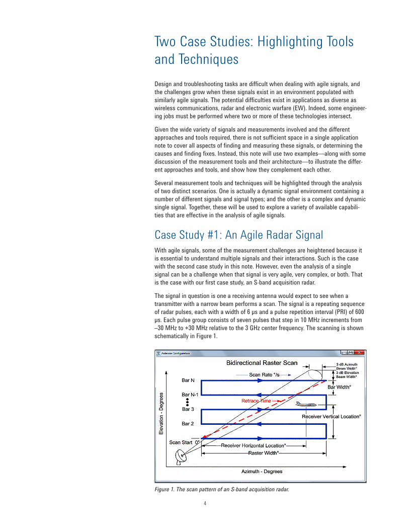
Case Study #1: An Agile Radar SignalWith agile signals, some of the measurement challenges are heightened because it is essential to understand multiple signals and their interactions. Such is the case with the second case study in this note. However, even the analysis of a single signal can be a challenge when that signal is very agile, very complex, or both. That is the case with our first case study, an S-band acquisition radar.

The signal in question is one a receiving antenna would expect to see when a transmitter with a narrow beam performs a scan. The signal is a repeating sequence of radar pulses, each with a width of 6 µs and a pulse repetition interval (PRI) of 600 µs. Each pulse group consists of seven pulses that step in 10 MHz increments from –30 MHz to +30 MHz relative to the 3 GHz center frequency. The scanning is shown schematically in Figure 1.

Figure 1. The scan pattern of an S-band acquisition radar.

5

The signal at the receiver varies widely in amplitude over a period of several seconds and this long-duration characteristic, combined with the short-duration characteristics of its pulse length and PRI (and therefore short duty cycle), make it agile and difficult to measure well.

Beyond max hold: density and persistence displaysA basic spectrum analysis of this signal with a swept spectrum analyzer reveals the measurement difficulty it poses, as shown in Figure 2. Even after many sweeps and the use of a max-hold function, the signal is not clearly represented. In fact, due to the max-hold function and the single-valued spectrum trace, the scanning (amplitude) dynamics of the signal are not represented at all. Some level of signal analysis is certainly possible in this mode but it is limited and requires considerable interpretation and the use of some assumptions. One additional measurement technique for signals such as this would be a zero-span measurement that uses a wide resolution bandwidth (RBW) filter and tuning of the analyzer to one of the signal peaks discovered in this display.

Figure 2. Even when using fast sweeps and max hold over a period of many seconds, the swept spectrum analyzer view of the radar signal is not very informative.

6

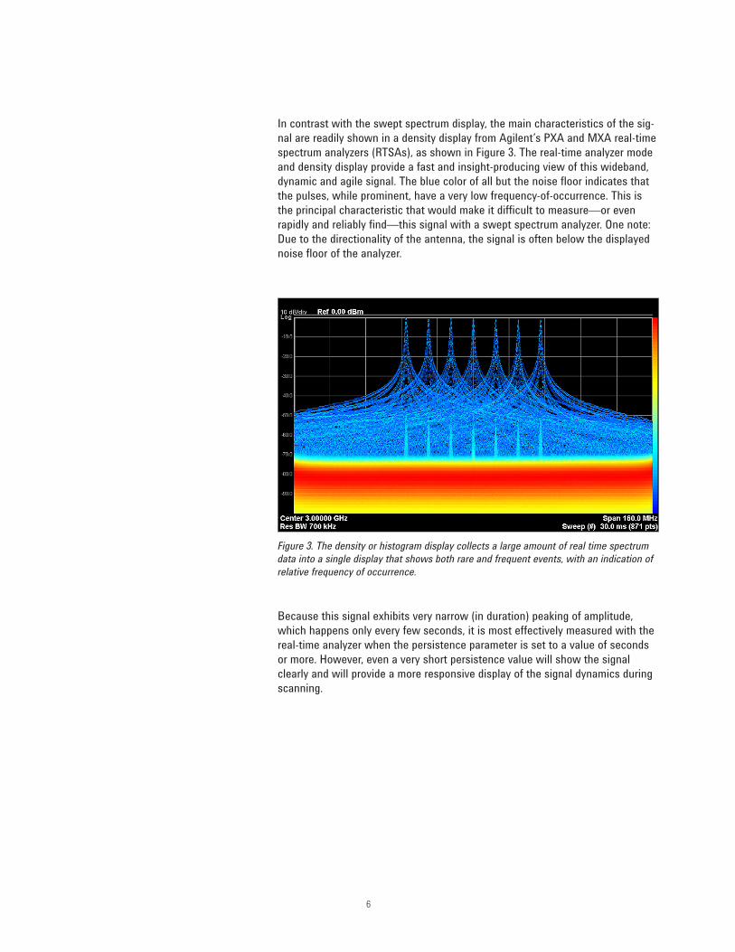
In contrast with the swept spectrum display, the main characteristics of the sig-nal are readily shown in a density display from Agilent’s PXA and MXA real-time spectrum analyzers (RTSAs), as shown in Figure 3. The real-time analyzer mode and density display provide a fast and insight-producing view of this wideband, dynamic and agile signal. The blue color of all but the noise floor indicates that the pulses, while prominent, have a very low frequency-of-occurrence. This is the principal characteristic that would make it difficult to measure—or even rapidly and reliably find—this signal with a swept spectrum analyzer. One note: Due to the directionality of the antenna, the signal is often below the displayed noise floor of the analyzer.

Because this signal exhibits very narrow (in duration) peaking of amplitude, which happens only every few seconds, it is most effectively measured with the real-time analyzer when the persistence parameter is set to a value of seconds or more. However, even a very short persistence value will show the signal clearly and will provide a more responsive display of the signal dynamics during scanning.

Figure 3. The density or histogram display collects a large amount of real time spectrum data into a single display that shows both rare and frequent events, with an indication of relative frequency of occurrence.

7

Figure 4. The spectrogram view of real-time data displays time information instead of density, providing a clear indication of signal behavior over time.

Changes over time: spectrogram displaysOne disadvantage of the density display is the lack of most information indicat-ing signal behavior over time. The density display itself can be observed over a period of time with an appropriate persistence value or even a range of persistence settings. Fortunately, real-time analyzers also provide spectrogram displays to take advantage of real-time spectral data, presenting spectrum vs. time vs. power rather than spectrum vs. density vs. power. An example spectro-gram of the radar signal is shown in Figure 4.

Spectrogram displays are increasingly common in mainstream signal analysis applications because they add a time dimension to the spectrum display. In real-time analyzers, they’re a complement to the density display. The display here is a real-time spectrogram in which individual real-time spectra (as shown at the top of the screen) are stacked vertically, with amplitude represented by color as shown at the left of the top display.

The individual spectrum lines are real-time but in most cases are formed from a number of individual FFT calculations (as controlled by the analyzer’s detector setting). In this configuration, each line represents about 10,000 FFT spectrum calculations.

8

Optimizing acquisition and persistence valuesTo optimize the spectrogram view over a period of seconds, the display in Figure 4 is configured for a long acquisition time and long persistence. This allows a distinct pattern to be identified, including medium-amplitude double peaks and higher-amplitude single peaks. Note, however, that a long persistence value in this display causes the signals to be blurred or smeared somewhat along the vertical time axis.

It is also important to note that each spectral line is composed of a large number of spectra, limiting the time resolution but increasing the time coverage of a single screen or spectrogram trace buffer. This characteristic result of measure-ment and display settings provides signal visibility at the cost of reduced time specificity. Thus, this display is more suited for observing signal behavior over a period of seconds rather than showing any individual pulses or pulse groups that characterize the signal behavior on the millisecond scale.

Because we may also want to observe (and perhaps verify) the pulse group behavior in the signal, it’s useful to shorten the acquisition and persistence val-ues. For brevity, some intermediate steps have been omitted: the display shown in Figure 5 has been optimized better for viewing the pulses only on a short time scale.

Figure 5. Large reductions in acquisition time and persistence optimize the real-time spec-trogram view for time resolution and display of brief events such as the pulse trains.

9

With a short acquisition time, each screen or spectrogram buffer (up to 10,000 traces in the Agilent RTSAs) provides much higher time resolution and a propor-tionally shorter coverage interval. Some amplitude variations related to antenna scanning can be seen near the signal peaks; however, the time scale of the signal changes is too long for this brief view and would be better shown with acquisition-time and persistence values in an intermediate range between those of Figures 4 and 5.

The greater time resolution of Figure 5 leads to visibility into what seem to be individual pulses or sets of pulses. The use of a spectrogram slice marker might be useful in this case but, because each spectrogram trace still represents multiple spectrum calculations, the relative timing would be difficult to see and could not be accurately measured. However, the view of the signal is much more detailed than previous ones and somewhat longer time periods could be viewed by viewing multiple spectrogram screens or scrolling through the large spectrogram buffer.

Shortening acquisition time is a good next step in understanding how signals behave over time, but it may not be enough for complete analysis of fast-chang-ing signals such as this one. In addition, a shorter acquisition time does not provide controllable overlap for precise timing analysis. In many cases, including this one, each real-time spectrum display update or spectrogram line combines many individual spectral measurements, limiting the accessible time resolution.

10

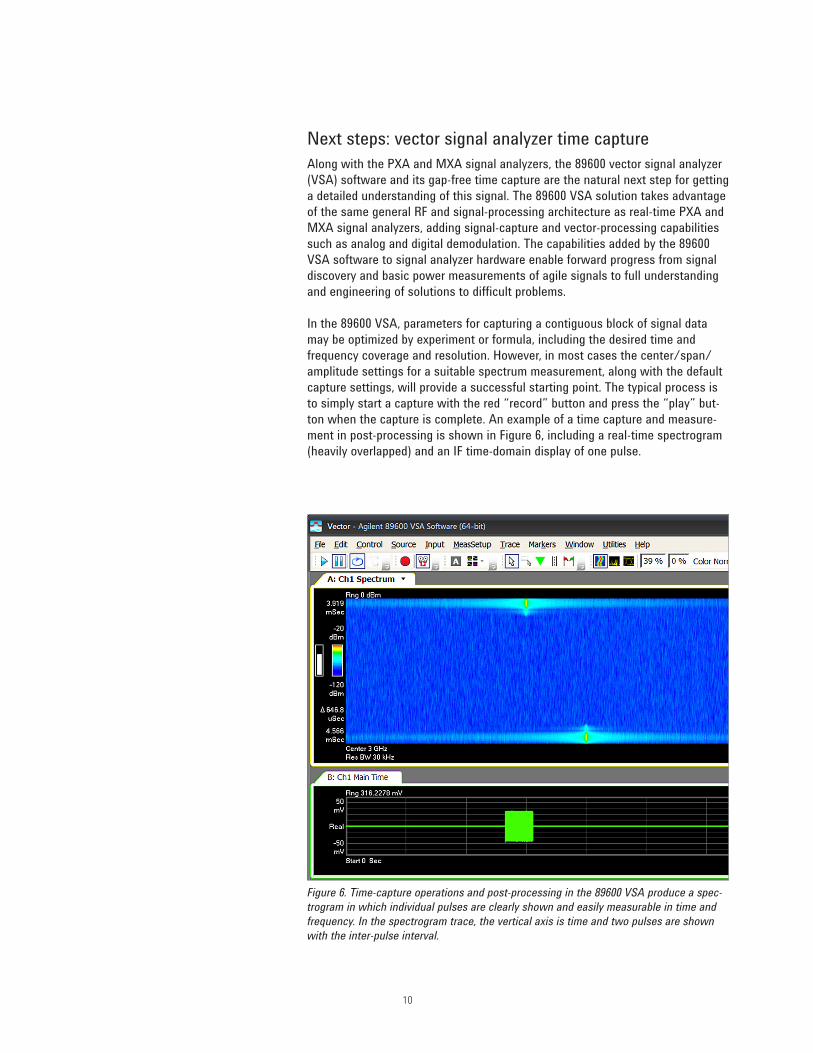
Next steps: vector signal analyzer time captureAlong with the PXA and MXA signal analyzers, the 89600 vector signal analyzer (VSA) software and its gap-free time capture are the natural next step for getting a detailed understanding of this signal. The 89600 VSA solution takes advantage of the same general RF and signal-processing architecture as real-time PXA and MXA signal analyzers, adding signal-capture and vector-processing capabilities such as analog and digital demodulation. The capabilities added by the 89600 VSA software to signal analyzer hardware enable forward progress from signal discovery and basic power measurements of agile signals to full understanding and engineering of solutions to difficult problems.

In the 89600 VSA, parameters for capturing a contiguous block of signal data may be optimized by experiment or formula, including the desired time and frequency coverage and resolution. However, in most cases the center/span/amplitude settings for a suitable spectrum measurement, along with the default capture settings, will provide a successful starting point. The typical process is to simply start a capture with the red “record” button and press the “play” but-ton when the capture is complete. An example of a time capture and measure-ment in post-processing is shown in Figure 6, including a real-time spectrogram (heavily overlapped) and an IF time-domain display of one pulse.

Figure 6. Time-capture operations and post-processing in the 89600 VSA produce a spec-trogram in which individual pulses are clearly shown and easily measurable in time and frequency. In the spectrogram trace, the vertical axis is time and two pulses are shownwith the inter-pulse interval.

11

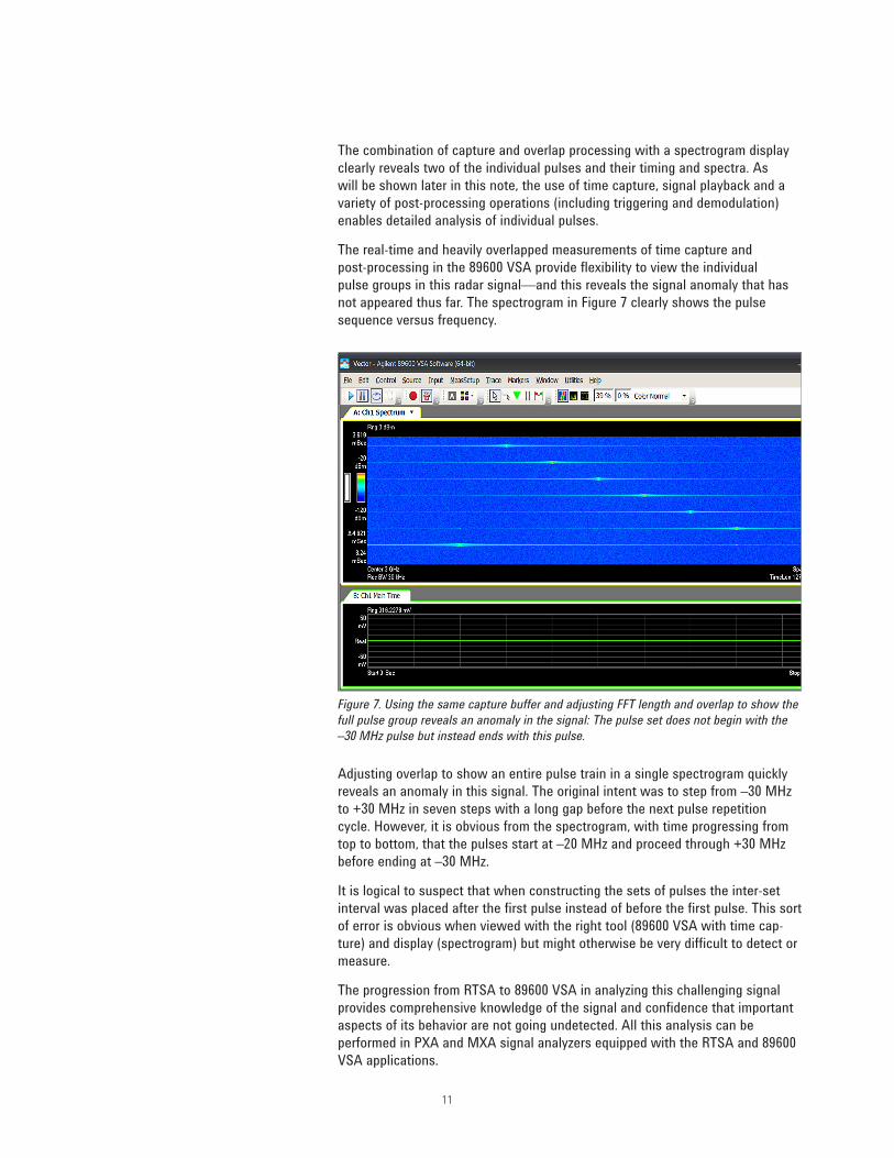
The combination of capture and overlap processing with a spectrogram display clearly reveals two of the individual pulses and their timing and spectra. As will be shown later in this note, the use of time capture, signal playback and a variety of post-processing operations (including triggering and demodulation) enables detailed analysis of individual pulses.

The real-time and heavily overlapped measurements of time capture and post-processing in the 89600 VSA provide flexibility to view the individual pulse groups in this radar signal—and this reveals the signal anomaly that has not appeared thus far. The spectrogram in Figure 7 clearly shows the pulse sequence versus frequency.

Adjusting overlap to show an entire pulse train in a single spectrogram quickly reveals an anomaly in this signal. The original intent was to step from –30 MHz to +30 MHz in seven steps with a long gap before the next pulse repetition cycle. However, it is obvious from the spectrogram, with time progressing from top to bottom, that the pulses start at –20 MHz and proceed through +30 MHz before ending at –30 MHz.

It is logical to suspect that when constructing the sets of pulses the inter-set interval was placed after the first pulse instead of before the first pulse. This sort of error is obvious when viewed with the right tool (89600 VSA with time cap-ture) and display (spectrogram) but might otherwise be very difficult to detect or measure.

The progression from RTSA to 89600 VSA in analyzing this challenging signal provides comprehensive knowledge of the signal and confidence that important aspects of its behavior are not going undetected. All this analysis can be performed in PXA and MXA signal analyzers equipped with the RTSA and 89600 VSA applications.

Figure 7. Using the same capture buffer and adjusting FFT length and overlap to show the full pulse group reveals an anomaly in the signal: The pulse set does not begin with the –30 MHz pulse but instead ends with this pulse.

12

Post-capture changes in center frequency and spanAs mentioned elsewhere in this note and described in detail in Case Study #2, it can be very useful to select portions of a capture buffer for detailed analysis in both the time and frequency domains. The traditional spectrum analyzer approach for RF engineers examining individual signals is to set the center frequency to the signal of interest and narrow the frequency span. This process is often referred to as “tune and zoom” and an example of the result on the captured radar signal is shown in Figure 8.

Figure 8. The same capture buffer is re-processed to focus analysis on a specific time and frequency region. In this measurement the center frequency is changed to match the +20 MHz pulse and the frequency span is reduced to 10 MHz. Gated sweep and a uniform window (for this self-windowing pulse) provide high-resolution analysis of a single selected pulse.

In this example, a single pulse is selected for analysis from the capture buffer. The time-record length has been set to a larger value of 50 µs but gated spectrum has been selected (the vertical green bars in the lower trace) with a uniform window (RBW filter) because the pulse signal is self-windowing. The result is shown in the upper trace.

Changing of the post-capture center frequency and span is supported in the 89600 VSA’s time capture and post-processing by DSP techniques (e.g., resampling) and a digital local oscillator (LO). Resampling of the sampled data—sometimes in combina-tion with decimation—provides a nearly infinite selection of effective sample rates from the original samples. This change in sample rates, combined with digital filtering, provides the reduced frequency spans that are desired. The result is analysis of the selected 10 MHz span around the signal of interest, with all signals outside of this span filtered out. The analysis is performed on the captured data already acquired, eliminating the need to re-tune the 89600 VSA and perform another capture.

Because the digital LO applied to the sampled data has changed the analysis center frequency, the new center frequency will apply to all measurements and can thus be used for operations such as analog or digital demodulation and changes in frequency resolution or RBW.

It is important to note that this “post-capture tune and zoom” capability is much more flexible and powerful than simply re-scaling or re-centering the spectrum data. Re-scaling spectrum display data would change only the display and would not support other analysis capabilities such as demodulation or changes in resolution or filtering.

13

Case Study #2: A Dynamic Signal EnvironmentCase Study #1 dealt with a single signal that was very agile. Another class of measurement challenges comes from complex signal environments, even if the signals they contain are not as agile.

Around the world, the industrial, scientific and medical (ISM) band at 2.45 GHz is perhaps the most varied and dynamic frequency band. In many locations it is lightly regulated and heavily used, and it has become especially popular for WLANs, Bluetooth® PANs, cordless phones, and RF heating devices such as high-power microwave ovens.

The band covers 100 MHz in many countries and spread spectrum techniques of some sort are often required for communications equipment. The two most popular techniques in the band are OFDM (used by 802.11g/n) and frequency hopping (Bluetooth); some cordless phones have used a simple form of CDMA.

Because the transmissions in this band are not generally coordinated, there are many opportunities for collisions and interference along with some complex interactions due to activities such as retransmissions. Fortunately, the modula-tion schemes and protocols used with these signals are designed to be some-what tolerant of collisions and interference.

The dynamics of the band are thus important for the objective of keeping data payloads moving, and some behaviors such as channel scanning may be a com-bination of brief (small fraction of a second), wideband (tens of MHz) and rare (occurring only every few seconds to minutes)—and this makes them difficult to see with traditional swept or FFT analyzer technologies. In these situations real-time analyzers can be very useful.

When unregulated bands become crowded and mutual interference increases significantly, there can be a rather sudden drop-off in total channel throughput, sometimes referred to as a cliff effect. At a certain channel loading, collisions and the increase in channel occupancy due to retransmissions can cause a cascade in which effective channel throughput is seriously impaired.

14

Beyond peak hold: density displaysThe 2.45 GHz ISM band is thus both dynamic and complex, and a good example of the challenges of agile signal analysis. Traditional swept spectrum analysis is not a very effective tool for understanding the activity in this band, as shown in Figure 9.

Depending on the degree of spectrum/time occupancy, a single sweep from a spectrum analyzer may show either nothing or only a portion of one or more signal bursts. It can be very difficult to interpret such a measurement, especially because the dynamics of the analyzer’s sweeping RBW filter interact with the dynamics of the signal itself.

Peak hold is a useful tool for understanding some aspects of the signal environ-ment, and a long measurement with peak hold will eventually catch most of the signals in the band. However, long peak-hold measurements often result in some signals in the band obscuring others as shown at the right in Figure 9.

Figure 9. With multiple agile signals sharing a 100 MHz frequency band, it can be difficult to understand signal behavior using a swept spectrum analyzer. Using the peak-hold function over a period of time can catch some signal activity but subsequent activity can also obscure it.

15

This density display from a real-time analyzer provides a good and immediate understanding of the ISM band and the signals in it. Because the measurements are gap-free and all signal samples are represented in the display in some fashion, it is possible to see most of the signals in the band at a glance or over a short measurement time.

The density or spectrogram display is very data-dense and quite dynamic, updating about 30 times per second and with some (adjustable) amount of persistence applied to fade older data. With an FFT rate of almost 300,000 per second, each display update represents about 10,000 spectra. The result is a responsive display that does a good job of keeping up with the dynamics of the in-band signals and showing subtle detail such as signals inside of other signals and small signals near the noise floor of the analyzer.

It is worth noting, however, that the action of combining 10,000 spectra into one display update can cause signals present at different times to be displayed in the same spectrum update. The signals that appear to be multi-tone in Figure 10 are actually Bluetooth frequency-hop patterns. The signal is never actually transmit-ted on multiple frequencies at once.

Figure 10. With a similar setup to the swept spectrum analysis approach (Figure 9) the real-time density display quickly reveals detail about the spectral occupancy of this band.

While swept spectrum analysis is not a productive way to understand the activ-ity in this band, the fast processing and advanced displays of real-time analyzers make them a good fit for exploring this dynamic signal environment, as shown in Figure 10.

16

Variations versus time: real-time spectrogram displaysAn alternative way to understand the signal behavior in this frequency band is to use a real-time spectrogram display, as described in Case Study #1 and Figure 4. The result is shown in Figure 11. With default settings, the spectrogram is a good way to view signal or environment behavior over a period of seconds. The combination of many spectra to form one spectrum update, and thus one hori-zontal line of the spectrogram, causes repeated Bluetooth hops over a limited channel pattern to form a set of vertical lines in the spectrogram display.

The time element (vertical axis) of the spectrogram can reveal important aspects of signal behavior in the spectral environment. Note that many Bluetooth hops form a repeating pattern (vertical lines) and other bursts appear to be isolated (mostly in the top half of the spectrogram). Also note the diagonal bars that move between the wide WLAN channels in the bottom half of the spectrogram. These appear to be from some sort of channel scanning and are occasionally, over intervals of seconds, visible in the density displays.

The acquisition-time setting at the upper right of the display controls how individual spectra are combined into spectrum updates (as shown in the top trace) and into individual spectrum lines to form the spectrogram display. A longer acquisition combines more spectra to form a spectrum update and causes the spectrogram to be updated more slowly. This allows a single spectrogram display to represent a longer time period.

Figure 11. The spectrogram display of the ISM band summarizes signal behavior over a period of seconds, revealing mostly WLAN and Bluetooth signals.

17

In this case, increased time resolution allows the individual WLAN bursts and Bluetooth hops to be much better resolved. As a result, two things become clear: even the Bluetooth hops that overlap the WLAN bursts in frequency often do not overlap in time, and collisions are not as frequent as the previous display would suggest. Note, however, that each spectrum line in the spectrogram and in the trace still represents hundreds of individual FFT results from the real-time measurement engine.

Figure 12. Selecting a shorter acquisition time period of 1 ms rather than 30 ms provides in-creased time resolution, revealing more about the structure of the WLAN bursts and Bluetooth hops. The spectrogram now represents a much shorter interval in time.

Because coverage of a long time period is a tradeoff for the spectrogram, selec-tion of a much shorter acquisition time for each update— spectrum display or spectrogram line—provides much better time resolution, as shown in Figure 12. The short acquisition time can have a large effect on the appearance and content of the spectrogram display or buffer. Although the buffer and display will cover a proportionally shorter span of time and therefore may not show some longer-term phenomena, the additional time resolution can reveal important spectral behavior that would otherwise be obscured.

18

Additional resolution: power versus time displaysAnother display type available in the real-time analyzer can be helpful in under-standing these signals: the power versus time (PVT) display. A real-time display of the total RF power in the signal environment can provide additional time resolution, as shown in Figure 13. The PVT display is useful for understanding pulse or burst duration directly. In this ISM band the WLAN bursts or frames are comparatively long while the Bluetooth hops are much shorter.

Figure 13. The real-time display of RF power vs. time (top) shows the total power in the ISM band, including a longer WLAN burst and short Bluetooth hops.

19

Extending signal analysis with a vector signal analyzerAs described so far, the real-time analyzer architecture, processing and displays are very powerful in detecting elusive signals or agile signal behavior and in understanding complex and dynamic signal environments. This is particularly true if the phenomenon in question is unknown or unexpected.

Of course, finding an elusive signal or event is often just one step in finding and solving problems, or in optimizing performance. In these cases, 89600 VSA software is a logical and powerful complement to a real-time analyzer solution.

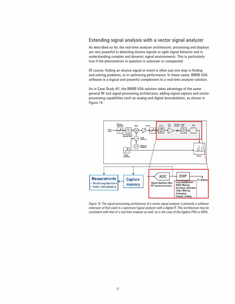
As in Case Study #1, the 89600 VSA solution takes advantage of the same general RF and signal-processing architecture, adding signal-capture and vector-processing capabilities such as analog and digital demodulation, as shown in Figure 14.

Figure 14. The signal-processing architecture of a vector signal analyzer is primarily a software extension of that used in a spectrum/signal analyzer with a digital IF. This architecture may be consistent with that of a real-time analyzer as well, as in the case of the Agilent PXA or MXA.

20

Vector signal analysis often begins with FFT analysis of a digitized IF signal. For agile signals or dynamic environments, FFT analysis has the benefit of removing one source of measurement variability or uncertainty: the sweeping RBW filter.

Because the entire spectrum measurement is calculated from a block or “time record” of the digitized IF signal, the data from which the spectrum is computed can be viewed and is well understood. In 89600 VSA software, the data used for the FFT can be further refined through the use of time gating, through which any portion of the time record can be selected for analysis. In addition, a window function for the gated spectrum can be independently selected to optimize the measurement.

In general, the default time record used in most analyzers is fairly short at about 1000 time samples; this is similar to the longest time records used in real-time analyzers. The resulting spectrum is shown at the top of Figure 15.

Fortunately, the time records in the 89600 VSA can be quite long. Longer time records provide a better view of many signals and a higher effective probability of intercept (POI), also shown in Figure 15. Using a long time record and enhanced displays such as persistence and density can result in signal views that are much more informative and significantly closer to real time, even though they are well short of genuine real-time analysis.

Using a long FFT time record (via the “# frequency points” setting in the 89600 VSA) results in much bigger contiguous blocks of analyzed time and increases the prob-ability of intercept. In the 89600 VSA, time-record length can be specified in terms of either time or number of points, depending on user preference.

Using persistence mode for displaying spectrum analysis results—either monochrome or color—causes information to remain on the display long enough to be seen and evaluated. Max-hold settings could achieve some of the same benefits; however, in many cases the accumulation of display results without discarding any can cause some to obscure others and limit the display’s responsiveness as the signal changes.

Figure 15. FFT analysis of a short time record (top) avoids the problem of the swept spec-trum analyzer’s moving RBW filter but POI is likely to be very low. For most agile signals, a more comprehensive view—and higher POI—is obtained through the use of a much longer time record (middle) and enhanced displays such as color persistence (bottom).

21

FFT analyzer settings to improve POIAs discussed earlier, the swept spectrum analyzer may not be the best way to characterize agile signals or dynamic signal environments. Fortunately, the adjustment of some basic 89600 VSA measurement settings can dramatically improve POI.

Use longer time records: Time-record length can be set in terms of seconds or frequency points. Because of overhead processing such as that involved in display updates, the spectrum update rate of the 89600 VSA generally decreases more slowly than the time-record length increases, so a higher percentage of ADC samples are processed with longer result lengths. One side benefit: longer time records include more signal dynamics. Those dynamics can be explored with gated sweep, which enables specific time portions of a signal to be later selected for spectrum analysis.

Reduce the frequency span: Because the effective ADC sample rate varies directly with frequency span, the POI increases as span is reduced. Thus, it is useful to reduce the measured frequency span—perhaps after the signal has been explored at a wider span—to the minimum necessary to measure the signal or frequency region in question.

Measure in a triggered mode: For some signals and signal environments, there are periods during which no signal (or no significant signal) is present. In such cases it is practical to set a magnitude threshold below which no time records are acquired and no measurement is made. The 89600 VSA’s magnitude trigger can easily accomplish this task, with the potential to dramatically improve POI simply by ensuring that no measurements are made when no signal is present. The negative trigger delay feature included in the 89600 VSA’s IF magnitude and frequency-mask triggers can be used to ensure that signals occurring before the trigger is satisfied are measurable as well. Of course, the use of the frequency-mask trigger (FMT) available with the real-time PXA and MXA along with the 89600 VSA combination can perform more sophisticated testing to ensure that only the desired signals are caught and measured. The FMT functionality will be described later in this note.

Use advanced, data-dense displays: Another approach to improving practical POI is to ensure that events that show up in even a single display update are not missed. In the 89600 VSA, the digital-persistence and cumulative-history display enhancements can readily provide this benefit, and can be customized as needed to highlight rare or frequent events or to differentiate between recent or older events.

These measurement settings and techniques may not provide the 100 percent POI that is available in a real-time analyzer; however, they can dramatically increase effective POI and allow the 89600 VSA to bring its wide range of sophisticated analysis capabilities to bear on difficult signals and measurements.

22

Triggering: Applying IF Magnitude & Frequency Mask to Case Study #2So far, FMT (spectral) and magnitude trigger types have been discussed only briefly. The following section will cover these in more detail, primarily in the context of the signal environment measurement of Case Study #2.

Both frequency-mask and IF-magnitude triggers operate on digital samples from the analyzer IF. Real-time analyzers typically implement FMT while vector signal analyzers have generally offered IF-magnitude triggering. With Agilent’s real-time PXA and MXA signal analyzers, the 89600 VSA can be used with the RTSA option to provide both FMT and IF-magnitude triggering.

Both trigger types employ ASICs, FPGAs, or both, to perform the real-time calcu-lations required for triggering. IF-magnitude triggering has been available for RF signals in vector signal analyzers for quite some time, beginning with the 89400 VSA instruments (c.1993). As with current signal analyzers such as the PXA and MXA, ASICs or FPGAs are used to calculate, in real time, the signal magnitude by taking the square root of the I2 + Q2 combination. These calculations are performed in real time on a sample-by-sample basis with time alignment, allow-ing triggers to be aligned with specific samples of the IF signal. In contrast, the FMT requires more processing power because the triggering is calculated on the basis of a spectrum result, which is transformed from a block of samples (as previously described).

In the 89600 VSA software, either type of trigger can be used to initiate an individual measurement or a time capture of a large block of samples that can be post-processed as desired. Positive and negative trigger delays can be applied to either trigger type to ensure that a complete signal event is available for measurement or post-processing.

23

FMT and the ISM bandWhen dealing with dynamic scenarios such as the ISM band, the FMT capability can be a very useful tool in finding signals—either expected or unexpected—and improving POI. For example, the FMT is a powerful way to take advantage of the very fast spectrum calculations inherent in real-time analyzers. As previously mentioned, the spectra are calculated much too rapidly to be viewed by users but it is not difficult for high-speed DSP to evaluate them individually against one or more spectral masks and against behavior criteria such as enter-then-leave-mask, etc. When the result of the evaluation is a measurement trigger, this provides an effective way to sort through millions or billions of spectra to find specific signals or events or circuit behavior (Figure 16).

In the example shown in Figure 16, the FMT is set up to detect when the WLAN radios are switching between channels or when another signal (such as a Bluetooth hop) appears between the WLAN channels. Normally, the WLAN signals stay within their typical three channels; however, as becomes apparent when watched for several seconds or longer, channel scanning may occur, especially when the ISM band is crowded. One note: an RF pulse or magnitude trigger would not work in this case because the scanning has a distinctive spec-tral shape but not a large magnitude (e.g., not larger than the rest of the signals in the analysis bandwidth).

Figure 16. A frequency mask constructed around three WLAN channels is violated when one WLAN transmitter switches to a frequency that is between channels currently in use.

24

Untriggered time capture and playback with the 89600 VSA might capture this event. However, because it happens comparatively rarely (e.g., every few seconds to tens of seconds) it could be missed or would be very tedious and time-consuming to find. For example, it might be quite tiresome to review a time capture of long enough duration to ensure a high probability of including the scanning event (high POI).

Because the trigger is generated from FFT power spectrum results, the basic trigger timing resolution is 1/FFT period (in units of time). In some cases it might be possible to further refine the timing; however, it is important to note that the trigger is asynchronous with the signal and not time-aligned with the signal’s RF envelope.

The frequency-mask trigger can be used in several different ways, the most com-mon being the initiation of a spectrum measurement or group of measurements. The trigger can also be used, in concert with 89600 VSA software, for vector measurements such as analog or digital demodulation. Also with the VSA soft-ware, the trigger can be used to start a time-capture operation to record a signal event (including the time before the trigger) for a wide range of post-processing operations including demodulation.

Selecting signals from the ISM band for analysis and demodulationThe combination of the real-time analyzer’s FMT and the 89600 VSA’s time-capture mode is especially useful for analyzing one or more of the abundant signals and events present in the ISM band. Because the content of the band is continuously changing, a significant benefit of time capture and post-processing is that analysis parameters, displays and analysis types can be changed while analyzing the same event over and over. This avoids situations with ambiguous interpretations in which the engineer cannot be sure if inconsistent analysis results are due to different analysis settings or to a change in the signal itself.

In the 89600 VSA, graphic tools simplify navigation of time-capture buffers and the selection of which portions to analyze. Playback begins at the start time and ends or repeats at the stop time, and the current analysis position in the buffer is shown both numerically and graphically. These parameters can be entered numerically or graphically.

One convenient approach is to drag the analysis position indicator while watch-ing the analysis displays to find the signal of interest and identify the desired start/stop times: the displays are updated continuously as the position is changed. The start/stop time sliders can then be moved to select the appropri-ate analysis region.

25

The spectrogram display is an excellent tool for understanding behavior in the ISM band and then selecting the signals and analysis region of interest. The crowded and complex character of the ISM band is shown in Figure 17: a cap-ture lasting about 26 ms and covering the entire band was occupied by energy from WLAN bursts, Bluetooth hops and microwave ovens.

Figure 17. This spectrogram display provides an overview of signals and behavior in the 2.45GHz ISM band over an interval of about 26 ms. The highly-overlapped real time measurement produces a detailed view of WLAN bursts, Bluetooth hops and microwave oven leakage.

Gap-free playback with adjustable overlap provides a detailed look at all activity in the band over time. Virtually any activity can be seen and measured and the horizontal spectrogram or slice markers can be used with a relative time marker to understand signal timing (see red ellipse, upper right of Figure 17). The 16.7 ms indicated time interval of repeating microwave oven bursts (the narrow curving lines) shows that they are operating on a 60-Hz cycle.

The fine time resolution of the spectra in the spectrogram reveals some instanc-es of interference and many of effective spectrum sharing. Note that, within this timeframe, two WLANS are successfully sharing the center channel. Also note that most Bluetooth hops are clear of WLAN bursts and oven activity.

Sharing of this band by multiple users appears to be successful, though one could imagine problems as the band gets busier. At some point, interference could cause excessive retransmissions and those additional bursts could lead to even more interference and retransmissions. This positive feedback situa-tion could lead to another cliff effect: small increments in band activity could cause large problems with effective throughput. The density and spectrogram displays of real-time analyzers would be useful in spotting this phenomenon and capture/playback and spectrogram displays from an 89600 VSA would be very useful in diagnosing problems and testing potential solutions.

26

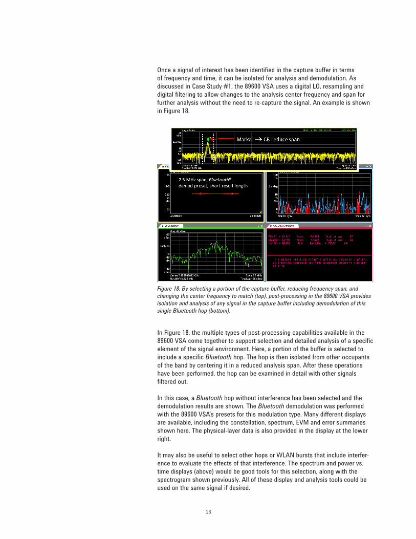
Once a signal of interest has been identified in the capture buffer in terms of frequency and time, it can be isolated for analysis and demodulation. As discussed in Case Study #1, the 89600 VSA uses a digital LO, resampling and digital filtering to allow changes to the analysis center frequency and span for further analysis without the need to re-capture the signal. An example is shown in Figure 18.

In Figure 18, the multiple types of post-processing capabilities available in the 89600 VSA come together to support selection and detailed analysis of a specific element of the signal environment. Here, a portion of the buffer is selected to include a specific Bluetooth hop. The hop is then isolated from other occupants of the band by centering it in a reduced analysis span. After these operations have been performed, the hop can be examined in detail with other signals filtered out.

In this case, a Bluetooth hop without interference has been selected and the demodulation results are shown. The Bluetooth demodulation was performed with the 89600 VSA’s presets for this modulation type. Many different displays are available, including the constellation, spectrum, EVM and error summaries shown here. The physical-layer data is also provided in the display at the lower right.

It may also be useful to select other hops or WLAN bursts that include interfer-ence to evaluate the effects of that interference. The spectrum and power vs. time displays (above) would be good tools for this selection, along with the spectrogram shown previously. All of these display and analysis tools could be used on the same signal if desired.

Figure 18. By selecting a portion of the capture buffer, reducing frequency span, and changing the center frequency to match (top), post-processing in the 89600 VSA provides isolation and analysis of any signal in the capture buffer including demodulation of this single Bluetooth hop (bottom).

27

Selecting and saving sampled data for RF output or other analysisA major benefit of the ability to find and measure agile signals is the potential for re-using them, either as real-world RF stimulus signals or as inputs to another process such as simulation or mathematics tools. This allows real-world signals, including their defects or impairments, to be used in other design and test processes.

In the 89600 VSA, selecting and saving time and frequency segments of captured data is straightforward, as shown in Figure 19. In the software, the sampled data from a measurement or time capture can be saved either as-is or in a modified form. For example, the data can be saved at an altered center frequency and span, after the operations of resampling and mixing with a digital LO, as described previously.

In addition, a particular time portion of the sampled data can be selected for saving, and this selection can be combined with the frequency conversion opera-tions. In the Figure 19 example, a shortened burst has been found, and the data portion has been measured with gated sweep. The shortened burst itself can be selectively saved or passed along to other processes for analysis, or used as an RF stimulus signal.

Figure 19. When storing a time-capture recording in the 89600 VSA, options are provided to save selected data between start/stop times, and to save data at center and span frequencies different than the original capture. These processing options make it easier to re-use sampled data in other instruments, tools or processes.

28

In real-time analyzers and vector signal analyzers, the combination of real-time analysis and density displays is especially useful for agile signals and dynamic spectral environments. When the signal or behavior in question is short in dura-tion, infrequent in occurrence, or simply unexpected, the large amount of data that can be processed and represented by a real-time analyzer can provide the best chance of detection.

While a real-time analyzer and its display capabilities are very useful, there are limits to its diagnostic or troubleshooting power. For example, the large amount of spectrum results compared to the limited rate of display updates means that each update typically combines many spectra. As a result, it may be hard to see, in any detail, those phenomena that have a rate of change much faster than the display update or acquisition time.

Vector signal analyzers are the logical complement and extension of the signal discovery functions of real-time analyzers. As shown in the examples here, the two analyzer types work together to take engineers from signal discovery and analysis of the most agile and challenging signals through the process of analy-sis, troubleshooting and optimization.

Both real-time analyzers and the 89600 VSA can operate on the hardware platform of swept analyzers such as the Agilent PXA and MXA, building on the performance, flexibility and familiar user interface of this fundamental RF analysis tool.

Summary

29

In many challenging situations, choosing and using a triggering approach from one of the several available can dramatically improve the effectiveness of your measurements. It can be used to focus your attention on the signals or time intervals that matter the most or are most likely to reveal troublesome signals. For example, selection of an appropriate trigger type and setting can ensure that the analyzer is not measuring when no signal is present and is therefore more likely to be armed and ready to measure or capture when significant signals appear.

Triggering can be especially helpful when examining long time periods for either expected or unexpected signals. The two trigger types discussed below both involve real-time calculations performed on the digitized signal and therefore can monitor signals or signal environments exhaustively in ways that are impractical for analyzer operators to duplicate visually.

For real-time analyzers and vector signal analyzers, the two most useful trigger types for agile RF signals are frequency-mask triggering and IF-magnitude trig-gering. Their benefits are summarized and compared in Table 1, below.

These triggering techniques are most effective when combined with specific knowledge of your signals or systems and with your insights into phenomena or behavior that are of most interest or concern. Be sure to consider all you know about important signal levels and transitions as well as relative timing of the signal of interest versus others. When using vector signal analyzers such as the 89600 VSA, be sure to consider positive and negative trigger delays and trigger holdoff as ways to measure a signal of interest, even if it is not the signal that initiates the trigger.

Table 1. Comparing IF magnitude and frequency-mask triggering techniquesIF Magnitude FMTReal-time calculation of magnitude in selected span

Real-time calculation of spectrum & test against spectral mask

Precise, repeatable time alignment Upper and lower limitsNegative & positive trigger delays Build from trace & adjust, or enter

parameters manually Selectable level & polarity Trigger timing ambiguity ±1 FFT periodSelectable holdoff, holdoff type Logic: Enter/leave, in/out,

enter → leave, leave → enterPlayback IF magnitude trigger Negative & positive trigger delays

Appendix: Comparing Triggering Techniques and Benefits

30

Consider time capture as alternative to triggeringWhen triggering is impractical or difficult, the time-capture and post-capture signal-selection capabilities of the 89600 VSA may be a useful alternative. For repeating signals, it may be practical to simply record a signal long enough to ensure that a full cycle, full pulse or complete frame is captured, and then select the appropriate measurement position or interval in post-processing.

The main element of this approach is to set the capture to an adequate length. For repeating pulsed or bursted signals, a general rule for the minimum is to set the capture length to a time equal to the sum of the inter-burst interval plus twice the burst length. This [“off time” + 2x “on time”] calculation would be the same for analyzing a digitally modulated burst or frame when you want the search time to always include the beginning, middle and end of a frame.

As described previously, the analysis region can be selected graphically or numerically to focus on the signal of interest. In a similar way, if a problem is repetitive and not especially rare, one may simply capture a segment of suffi-cient length and look for the signal or event of interest during playback. In some cases, this approach is actually easier than setting up other trigger types. It may also be useful when spectral characteristics of interest are not known, either as spectrum shape or behavior over time. Note that because this approach is simply a form of time capture, the results are always gap-free and analysis types and parameters can be freely changed in post-processing.

www.agilent.comwww.agilent/find/RTSA

Bluetooth® and the Bluetooth logos are trade-marks owned by Bluetooth SIG, Inc, U.S.A. and licensed to Agilent Technologies, Inc.

www.agilent.com/quality

www.lxistandard.orgLAN eXtensions for Instruments puts the power of Ethernet and the Webinside your test systems. Agilent is a founding member of the LXI consortium.

Agilent Channel Partnerswww.agilent.com/find/channelpartnersGet the best of both worlds: Agilent’s measurement expertise and product breadth, combined with channel partner convenience.

www.agilent.com/find/myagilentA personalized view into the information most relevant to you.

myAgilent

www.agilent.com/find/AdvantageServicesAccurate measurements throughout the life of your instruments.

Agilent Advantage Services

Three-Year Warranty

www.agilent.com/find/ThreeYearWarrantyAgilent’s combination of product reliability and three-year warranty coverage is another way we help you achieve your business goals: increased confidence in uptime, reduced cost of ownership and greater convenience.

For more information on Agilent Technologies’ products, applications or services, please contact your local Agilent office. The complete list is available at:www.agilent.com/find/contactus

Americas Canada (877) 894 4414 Brazil (11) 4197 3600Mexico 01800 5064 800 United States (800) 829 4444

Asia Pacific Australia 1 800 629 485China 800 810 0189Hong Kong 800 938 693India 1 800 112 929Japan 0120 (421) 345Korea 080 769 0800Malaysia 1 800 888 848Singapore 1 800 375 8100Taiwan 0800 047 866Other AP Countries (65) 375 8100

Europe & Middle EastBelgium 32 (0) 2 404 93 40 Denmark 45 45 80 12 15Finland 358 (0) 10 855 2100France 0825 010 700* *0.125 €/minuteGermany 49 (0) 7031 464 6333 Ireland 1890 924 204Israel 972-3-9288-504/544Italy 39 02 92 60 8484Netherlands 31 (0) 20 547 2111Spain 34 (91) 631 3300Sweden 0200-88 22 55United Kingdom 44 (0) 118 927 6201For other unlisted countries: www.agilent.com/find/contactus(BP-3-1-13)

Product specifications and descriptions in this document subject to change without notice.

© Agilent Technologies, Inc. 2013Published in USA, May 23, 20135991-2119EN