measurements of sub-degree b-mode polarization in …

MEASUREMENTS OF SUB-DEGREE B-MODE POLARIZATION IN THE COSMIC MICROWAVEBACKGROUND FROM 100 SQUARE DEGREES OF SPTPOL DATA

R. Keisler1,2, S. Hoover

3,4, N. Harrington

5, J. W. Henning

3,6, P. A. R. Ade

7, K. A. Aird

8, J. E. Austermann

6,9, J. A. Beall

9,

A. N. Bender3,10,11

, B. A. Benson3,12,13

, L. E. Bleem3,4,11

, J. E. Carlstrom3,4,11,12,14

, C. L. Chang3,11,12

, H. C. Chiang15,

H-M. Cho16, R. Citron

3, T. M. Crawford

3,12, A. T. Crites

3,12,17, T. de Haan

5, M. A. Dobbs

10,18, W. Everett

6, J. Gallicchio

3,

J. Gao9, E. M. George

5, A. Gilbert

10, N. W. Halverson

6,19, D. Hanson

10, G. C. Hilton

9, G. P. Holder

10, W. L. Holzapfel

5,

Z. Hou3, J. D. Hrubes

8, N. Huang

5, J. Hubmayr

9, K. D. Irwin

1,16, L. Knox

20, A. T. Lee

5,21, E. M. Leitch

3,12, D. Li

9,16,

D. Luong-Van8, D. P. Marrone

22, J. J. McMahon

23, J. Mehl

3,11, S. S. Meyer

3,4,12,14, L. Mocanu

3,12, T. Natoli

3,4,

J. P. Nibarger9, V. Novosad

25, S. Padin

17, C. Pryke

26, C. L. Reichardt

5,27, J. E. Ruhl

24, B. R. Saliwanchik

24, J. T. Sayre

24,

K. K. Schaffer3,14,28

, E. Shirokoff3,12

, G. Smecher10,29

, A. A. Stark30, K. T. Story

3,4, C. Tucker

7, K. Vanderlinde

31,32,

J. D. Vieira33,34

, G. Wang11, N. Whitehorn

5, V. Yefremenko

11, and O. Zahn

35

1 Department of Physics, Stanford University, 382 Via Pueblo Mall, Stanford, CA 94305, USA; [email protected] Kavli Institute for Particle Astrophysics and Cosmology, Stanford University, 452 Lomita Mall, Stanford, CA 94305, USA

3 Kavli Institute for Cosmological Physics, University of Chicago, 5640 South Ellis Avenue, Chicago, IL 60637, USA4 Department of Physics, University of Chicago, 5640 South Ellis Avenue, Chicago, IL 60637, USA

5 Department of Physics, University of California, Berkeley, CA 94720, USA6 Department of Astrophysical and Planetary Sciences, University of Colorado, Boulder, CO 80309, USA

7 School of Physics and Astronomy, Cardiff University, CF24 3AA, UK8 University of Chicago, 5640 South Ellis Avenue, Chicago, IL 60637, USA

9 NIST Quantum Devices Group, 325 Broadway Mailcode 817.03, Boulder, CO 80305, USA10 Department of Physics, McGill University, 3600 Rue University, Montreal, Quebec H3A 2T8, Canada

11 High Energy Physics Division, Argonne National Laboratory, 9700 S. Cass Avenue, Argonne, IL 60439, USA12 Department of Astronomy and Astrophysics, University of Chicago, 5640 South Ellis Avenue, Chicago, IL 60637, USA

13 Fermi National Accelerator Laboratory, MS209, P.O. Box 500, Batavia, IL 60510, USA14 Enrico Fermi Institute, University of Chicago, 5640 South Ellis Avenue, Chicago, IL 60637, USA

15 School of Mathematics, Statistics & Computer Science, University of KwaZulu-Natal, Durban, South Africa16 SLAC National Accelerator Laboratory, 2575 Sand Hill Road, Menlo Park, CA 94025, USA

17 California Institute of Technology, MS 367-17, 1200 E. California Blvd., Pasadena, CA 91125, USA18 Canadian Institute for Advanced Research, CIFAR Program in Cosmology and Gravity, Toronto, ONM5G 1Z8, Canada

19 Department of Physics, University of Colorado, Boulder, CO 80309, USA20 Department of Physics, University of California, One Shields Avenue, Davis, CA 95616, USA

21 Physics Division, Lawrence Berkeley National Laboratory, Berkeley, CA 94720, USA22 Steward Observatory, University of Arizona, 933 North Cherry Avenue, Tucson, AZ 85721, USA23 Department of Physics, University of Michigan, 450 Church Street, Ann Arbor, MI 48109, USA

24 Physics Department, Center for Education and Research in Cosmology and Astrophysics,Case Western Reserve University, Cleveland, OH 44106, USA

25 Materials Sciences Division, Argonne National Laboratory, 9700 S. Cass Avenue, Argonne, IL 60439, USA26 School of Physics and Astronomy, University of Minnesota, 116 Church Street SE, Minneapolis, MN 55455, USA

27 School of Physics, University of Melbourne, Parkville, VIC 3010, Australia28 Liberal Arts Department, School of the Art Institute of Chicago, 112 S. Michigan Avenue, Chicago, IL 60603, USA

29 Three-Speed Logic, Inc., Vancouver, BCV6A 2J8, Canada30 Harvard-Smithsonian Center for Astrophysics, 60 Garden Street, Cambridge, MA 02138, USA

31 Dunlap Institute for Astronomy & Astrophysics, University of Toronto, 50 St George Street, Toronto, ONM5S 3H4, Canada32 Department of Astronomy & Astrophysics, University of Toronto, 50 St George Street, Toronto, ONM5S 3H4, Canada33 Astronomy Department, University of Illinois at Urbana-Champaign, 1002 W. Green Street, Urbana, IL 61801, USA34 Department of Physics, University of Illinois at Urbana-Champaign, 1110 W. Green Street, Urbana, IL 61801, USA

35 Berkeley Center for Cosmological Physics, Department of Physics, University of California,and Lawrence Berkeley National Laboratory, Berkeley, CA 94720, USAReceived 2015 March 9; accepted 2015 May 28; published 2015 July 9

ABSTRACT

We present a measurement of the B-mode polarization power spectrum (the BB spectrum) from 100 deg2

of sky observed with SPTpol, a polarization-sensitive receiver currently installed on the South Pole Telescope.The observations used in this work were taken during 2012 and early 2013 and include data in spectralbands centered at 95 and 150 GHz. We report the BB spectrum in five bins in multipole space, spanningthe range ℓ300 2300⩽ ⩽ , and for three spectral combinations: 95 GHz × 95 GHz, 95 GHz × 150 GHz,and 150 GHz × 150 GHz. We subtract small (<0.5σ in units of statistical uncertainty) biases from thesespectra and account for the uncertainty in those biases. The resulting power spectra are inconsistent with zeropower but consistent with predictions for the BB spectrum arising from the gravitational lensing of E-modepolarization. If we assume no other source of BB power besides lensed B modes, we determine a preference forlensed B modes of 4.9σ. After marginalizing over tensor power and foregrounds, namely, polarized emission fromgalactic dust and extragalactic sources, this significance is 4.3σ. Fitting for a single parameter, Alens, that multipliesthe predicted lensed B-mode spectrum, and marginalizing over tensor power and foregrounds, we find

The Astrophysical Journal, 807:151 (18pp), 2015 July 10 doi:10.1088/0004-637X/807/2/151© 2015. The American Astronomical Society. All rights reserved.

1

mailto:[email protected]

http://dx.doi.org/10.1088/0004-637X/807/2/151

A 1.08 0.26lens = , indicating that our measured spectra are consistent with the signal expected fromgravitational lensing. The data presented here provide the best measurement to date of the B-mode power spectrumon these angular scales.

Key words: cosmic background radiation – cosmology: observations

1. INTRODUCTION

Measurements of the cosmic microwave background(CMB), the oldest light in the universe, contain a wealth ofcosmological information, informing our understanding ofphysical processes across nearly all of cosmic time (see Hu &Dodelson 2002 for a review). The majority of CMB photonslast interacted electromagnetically with matter at the epoch ofrecombination (z ∼ 1000), and it is that period of cosmichistory that is most tightly constrained by CMB observations.However, the interaction between CMB photons and matter atlower redshifts encodes information about the more recenthistory of the universe. In particular, the bending of CMBphoton trajectories due to gravitational lensing enablesreconstruction of the gravitational potential between recombi-nation and z = 0. Furthermore, the imprint of gravitationalwaves on the polarization of the CMB has the potential toprobe the absolute earliest moments of cosmic time.

Current CMB-derived constraints on cosmological para-meters rely primarily on information from the angular powerspectrum of the CMB temperature fluctuations (the TTspectrum;e.g., Planck Collaboration et al. 2014b). However,the polarization of the CMB holds a wealth of potentialinformation that is just beginning to be exploited. As with anyheadless vector field on the sphere, the linear polarization of theCMB36 can be decomposed into a curl-free component and adivergence-free component, often called “E modes” and “Bmodes,” respectively, after the analogous fields in electro-dynamics. The primary mechanism responsible for CMBpolarization is Thomson scattering between electrons andCMB photons with an anisotropic temperature distribution(e.g., Hu & White 1997). Scalar density perturbations at theepoch of recombination produce only E-mode polarization tofirst order via this mechanism. B-mode polarization in the CMBcan be produced by vector perturbations (primordial vorticity)or tensor perturbations (gravitational waves) and by thedistortion of E modes through gravitational lensing by matterbetween the last scattering surface and the observer (Kamion-kowski et al. 1997; Seljak & Zaldarriaga 1997; Zaldarriaga &Seljak 1998).

The search for B-mode polarization in the CMB has been atopic of particular interest because the most successful modelfor explaining many of the observed features of the universe,the paradigm of cosmic inflation, predicts the existence of abackground of gravitational waves (e.g., Abazajianet al. 2015a). These gravitational waves leave their imprinton the CMB through scattering at the epoch of recombination(and again at the epoch of reionization) through a contributionto the temperature, E-mode polarization, and—most impor-tantly—B-mode polarization of the CMB. The gravity-wavecontribution to the temperature and E-mode power spectra isalready constrained to be too small to measure (owing tocosmic variance;see, e.g., Planck Collaboration XVI 2014); B-mode polarization is the only window for measuring this signal

in the CMB. The amplitude of the gravitational-wave back-ground is proportional to the expansion rate during inflation,and hence to the energy scale of the inflationary potential.Thus, a measurement of primordial B-mode polarization in theCMB could potentially probe physics at energies approachingthe Planck scale.The CMB B modes induced by gravitational lensing of

primordial E modes are both an interesting signal in their ownright and a potential contaminant to the inflationary gravita-tional-wave (IGW) B modes. In general, the signature oflensing in the temperature and polarization of the CMB can beused to reconstruct the projected gravitational potential ϕbetween the observer and the last scattering surface (e.g.,Seljak & Zaldarriaga 1999). The reconstructed potential issensitive to the evolution of large-scale structure. In particular,massive neutrinos affect the shape of this potential bystreaming out of small-scale gravitational perturbations anddamping the growth of structure on these scales. A high-fidelitymeasurement of CMB lensing can in principle measure the sumof the neutrino masses (e.g., Abazajian et al. 2015b). Theestimate of ϕ from CMB lensing can also be used, in concertwith a highsignal-to-noise ratio map of the E modes, to predictthe B-mode lensing signal. The predicted B-mode lensingsignal can then be cross-correlated with a direct B-modemeasurement, as in, e.g., Hanson et al. (2013, hereafter H13),or can be used to clean the lensing B modes from a direct B-mode measurement, thereby improving sensitivity to IGW Bmodes (Kesden et al. 2002; Knox & Song 2002).Significant experimental progress has been made recently in

the field of CMB B modes. The first detection of B modes(H13) was made in cross-correlation, using CMB data fromSPTpol (Austermann et al. 2012)—a polarization-sensitivereceiver currently installed on the 10 m South Pole Telescope(SPT;Carlstrom et al. 2011)—and cosmic infrared background(CIB) data from Herschel-SPIRE (Griffin et al. 2010). Similarcross-correlation measurements have since been made(POLARBEAR Collaboration 2014b; van Engelenet al. 2014; Planck Collaboration et al. 2015) using CMB datafrom POLARBEAR (Arnold et al. 2010), ACTPol (Niemacket al. 2010), and the Planck satellite. The POLARBEAR teamalso published a measurement of the B-mode angular powerspectrum (POLARBEAR Collaboration 2014a) in which ∼2σevidence for the lensing signal was seen. Finally, BICEP2Collaboration (2014) reported a strong detection of BB power,including a component in excess of the ΛCDM prediction forlensing B modes at ℓ ∼ 80. The excess has been confirmed inyet deeper 150 GHz data on the same area of sky from the KeckArray experiment (Keck Array & BICEP2 Collaborationset al. 2015), but a recent joint analysis of BICEP2, Keck, andPlanck data (BICEP2/Keck & Planck Collaborationset al. 2015) has demonstrated that at least half of the excessis due to polarized emission from galactic dust and that theresidual power is consistent with zero IGW signal. Regardlessof the interpretation of the excess B-mode signal, this analysisreported a 7σ detection of lensing B modes at ℓ ∼ 200, thetightest direct measurement of lensing B modes to date.

36 The circular polarization of the CMB is observed to be extremely small, asexpected. See, e.g., Mainini et al. (2013).

2

The Astrophysical Journal, 807:151 (18pp), 2015 July 10 Keisler et al.

In this paper, we present a measurement of the BB spectrumin the multipole range ℓ300 2300⩽ ⩽ , estimated from100 deg2 of data taken with SPTpol in 2012 and 2013. Thedata used in this work have significant overlap with the dataused to make the first detection of B modes in H13, but thereare several key differences in the two data sets and analyses.First and most importantly, the analysis in H13 detected Bmodes in SPTpol data by cross-correlating SPTpol B-modemaps with a predicted B-mode template constructed using the Emodes measured with SPTpol and an estimate of ϕ from theCIB. Cross-correlation analyses have the attractive propertythat any systematic effect present in only one of the data setswill not bias the result. From a systematics perspective, the BBspectrum presented here is a much more challenging measure-ment than the H13 cross-correlation measurement, and theresults presented here demonstrate that SPTpol cleanlymeasures the B-mode power spectrum at angular scales oftens of arcmin. Furthermore, the B modes measured in H13 arenecessarily restricted to the lensing signal induced by the partof ϕ traced by the CIB (the CIB is expected to have good butnot perfect redshift overlap with the CMB lensing kernel;see,e.g., Holder et al. 2013). The BB spectrum presented in thiswork is sensitive to all contributing signals, including the fulllensing signal, the IGW signal (though no detection of IGW Bmodes is expected in the ℓ range probed in this work at thecurrent levels of sensitivity), and any foreground contamina-tion. This work also contains 95 and 150 GHz data from both2012 and early 2013, while H13 focused primarily on 150 GHzdata and used only 2012 data.

This paper is structured as follows: Section 2 describes thetelescope and receiver. Section 3 describes the observationsused in this analysis. Section 4 details the data reductionprocess from the raw, time-ordered detector data to the stage ofsingle-observation maps. Section 5 describes how we calculatethe power spectrum, including identifying and correcting forbiases in the measured BB spectrum, and presents the measuredspectrum. We interpret the results in the context of cosmologyand other B-mode and lensing results in Section 6, and weconclude in Section 7.

2. TELESCOPE AND RECEIVER

The SPT is a 10 m telescope with a wide field of view (∼1square degree at 150 GHz), designed for conducting large-areasurveys of fluctuations in the temperature and polarization ofthe CMB. The telescope is described in detail in Carlstromet al. (2011), and further details about the optical design can befound in Padin et al. (2008).

After five years of observation with the original SPT-SZreceiver, which was sensitive to the CMB intensity but not itspolarization, the polarization-sensitive SPTpol receiver wasinstalled in 2012. SPTpol is equipped with 1536 polarization-sensitive transition edge sensor (TES) bolometers, with 1176detectors at 150 GHz and 360 detectors at 95 GHz. Thedetectors in the two bands were designed and fabricatedindependently and are described in detail in Henning et al.(2012, 150 GHz) and Sayre et al. (2012, 95 GHz). The150 GHz array is composed of seven detector modules, eachcontaining 84 pixels, all fabricated at the National Institute forStandards and Technology Boulder Laboratory. Each moduleconsists of a detector array behind a monolithic feedhorn array.Incoming power is coupled through the feedhorns to anorthomode transducer, which splits the light into two

orthogonal polarization states. The 95 GHz array consists of180 individually packaged dual-polarization absorber-coupledpolarimeters (a total of 360 detectors) fabricated at ArgonneNational Laboratories. Each pair of 95 GHz detectors iscoupled to the telescope through machined contoured feed-horns. The detectors in both observing bands are read out usinga digital frequency-domain multiplexer system with cryogenicsuperconducting quantum interference device (SQUID)amplifiers.The focal plane is cooled to ∼250 mK using a commercial

pulse-tube cooler and a three-stage helium refrigerator. TheTES detectors are then biased to their operating point of∼500 mK. The entire receiver is maintained at ∼4 K, similar tothe SPT-SZ receiver described in Carlstrom et al. (2011). Thesecondary optics (including the secondary mirror cryostat) areidentical to those used for SPT-SZ, with the exception ofdifferent heat-blocking filters near the prime focus. Foradditional details on the SPTpol instrument design, seeAustermann et al. (2012).

3. OBSERVATIONS

The first 8 months of observing with the SPTpol receiver(2012 April–October and 2013 April) were dedicated primarilyto observations of a 100 deg2 patch of sky centered at R.A.23h30m and decl. −55°. We refer to this field as the SPTpol“100d” field to distinguish it from the 500 deg2 survey field, forwhich observations began in 2013 May. The 95 and 150 GHzdata from the first year (2012) of observations of the 100d fieldwere used in H13. The 150 GHz data from 2012 were also usedto compute the E-mode power spectrum (EE) and thetemperature-E-mode correlation spectrum (TE) in Crites et al.(2015, hereafter C15). Story et al. (2014) used the 150 GHzdata from both years of observation of this field to reconstructthe CMB lensing potential and analyze its power spectrum. Theanalysis presented here is the first to use the 95 and 150 GHzdata on this field from both years, and the effective white-noiselevels are approximately 17 and 9 μK arcmin in polarization at95 and 150 GHz, respectively.Some minor modifications to the instrument were made

between the 2012 and 2013 observing seasons that could affectthe analysis in this work. At 150 GHz, one detector module wasreplaced, and the filters used to define the band edges werereplaced in both bands. Both of these modifications mostdirectly affect the shape and overall width of the observingbands, which can in turn affect beam shape and absolutecalibration. For this reason, we estimate beams and absolutecalibration independently for both seasons.All observations of the 100d field used a constant-elevation

scan strategy, in which the telescope is slewed in azimuth backand forth once and then stepped a small amount in elevation,with the process repeated until the full elevation range iscovered. The azimuthal scanning speed used in all observationswas 0.48 degrees per second, corresponding to 0.28 degrees persecond on the sky at the mean elevation of the field, and theconstant-velocity portions of the scans were between 8 ◦. 8 and10 ◦. 75 in azimuth. The elevation step between scans wasbetween 13 and 20 arcmin.Only one-half of the azimuthal extent of the field is observed

at one time, in a “lead-trail” strategy that allows for groundcontamination to be efficiently subtracted when maps of thetwo field halves are differenced (e.g., Pryke et al. 2009). Sinceno ground signal is detected in this analysis (see Section 5.8.2)

3


or in C14, we do not use a lead-trail differencing analysis inthis work; instead, we simply combine each pair of half-fieldmaps into a map of the full field.

We refer to one pass of the telescope, either from left to rightor from right to left across half of the field, as a “scan,” and werefer to a set of scans that cover an entire half-field as an“observation.” Each observation lasts 30 minutes, and there area total of roughly 12,000 observations in the 2012 and 2013observing seasons, for a total of roughly 6000 individual-observation maps of the full field.

4. DATA REDUCTION: TIME-ORDERED DATA TO MAPS

In their raw form, the time-ordered data for each observationused in this work consist of one vector of uncalibrated ADCcounts for each detector, representing the current through theTES as a function of time, and two vectors representing thedetector pointing as a function of time. The first step inprocessing these data into angular power spectra is to convertthe time-ordered data into pixelized maps of the Stokesparameters I (or T for “temperature”), Q, and U on the sky. Theprocess used in this work for making maps from time-ordereddata closely follows that of C14; we describe the stages of thisprocess and point out any differences with C14 below.

4.1. Time-ordered Data Filtering

The data from each detector in each observation are filteredprior to making maps for a number of reasons: to removemodes that are strongly affected by low-frequency noise, toprevent aliasing of high-frequency noise to lower frequencieswhen the data are binned into map pixels, and to eliminatepotential contamination from detector coupling to the pulse-tube cooler used to cool the receiver. Data from each detectorin each scan are fit to a combination of a first-order polynomial(mean and slope) and a set of low-order Fourier modes (sinesand cosines). The best-fit polynomial and Fourier modes areremoved, resulting in an effective high-pass filter. When mapsare made from data filtered in this way, the effect of this time-domain filtering is a high-pass filter along the scan direction(equivalent to R.A. for observations from the South Pole) witha cutoff at angular scales of roughly 3° (or an effectivemultipole number in the scan direction of ℓ 100x ~ ).37 Toavoid filtering artifacts around bright point sources, all sourcesabove 50 mJy in unpolarized flux at 150 GHz are masked in thefitting process. An anti-aliasing low-pass filter is also applied tothe data from each detector on each scan, resulting in a scan-direction low-pass filter in the maps with a cutoff of ℓ 6600x ~ .This filter cutoff is set by the size of the pixels used inmapmaking, which is 1 arcmin for this analysis. A frequency-domain filter with very narrow notches at the pulse-tube coolerfrequency (and the second and third harmonics of thisfrequency) is applied to the data from each detector over theentire observation. A total of <0.01 Hz of bandwidth (<0.2% ofthe ℓ 6600x < band) is removed with this filter, and we do notinclude its effect in the simulations of the filter transfer functiondescribed in Section 5.1.

The C14 analysis used slightly different filtering choices.The scan-direction high-pass filtering was accomplished in C14using polynomial subtraction only (no Fourier modes); for this

work, we found that the combination of polynomials andFourier modes resulted in a lower level of spurious B-modepower created in the filtering step (see Section 5.5.1 fordetails). The anti-aliasing low-pass filter in C14 had a cutoff atℓ 10,000x ~ , because the maps used in that analysis had0.5 arcmin pixels.

4.2. Relative Calibration

Before the data from all detectors are combined into T, Q,and U maps, a factor is applied to the data from each detector toequalize the response to astronomical signal across each of thetwo detector arrays (95 and 150 GHz). The process ofmeasuring and monitoring this relative calibration for eacharray is identical to the process described in C14 and used inearlier SPT analyses (see Schaffer et al. 2011); we describe theprocess briefly here.The relative calibration process involves regular observa-

tions of the galactic H II region RCW38 and of an internalchopped blackbody source. A 45-minute observation of thegalactic H II region RCW38 is conducted approximately onceper day (shorter observations for pointing reconstruction areconducted more frequently), while 1-minute observations ofthe internal source are conducted at least once per hour. Aneffective temperature for the internal source is assignedindividually for each detector (by comparing to the seasonaverage of response to RCW38). This value times the responseof each detector to the internal source in the observation nearesta CMB field observation is used for relative calibration. Weassume that RCW38 is unpolarized, and internal measurementssuggest that it is <1% polarized. In Section 5.9.3 we discuss thepotential for spurious B-mode polarization caused by smallpolarization in RCW38.Drifts in the internal source temperature are accounted for by

comparing the average source response across a detectormodule38 in each observation to the module average over theentire season. Drifts in atmospheric opacity are addressedsimilarly using average RCW38 responses for each module.

4.3. Polarization Calibration

Before combining the data from all detectors into T, Q, andU maps, we must know the polarization properties of thedetectors. Each detector is designed to be sensitive to linearlypolarized radiation at a particular angle and insensitive toradiation in the orthogonal polarization. The two numbersrequired to characterize each detector’s polarization perfor-mance are the polarization angle θ (the angle of linearlypolarized radiation at which the response of the detector ismaximized) and the polarization efficiency ηp (a measure of theratio of detector response to linearly polarized radiation at θ toradiation polarized at 2q p+ ).These properties are measured for each detector in dedicated

observations of a polarized calibration source during theAustral summer season. The calibration observations and themethod by which θ and ηp are derived from the data aredescribed in detail in C14. We briefly summarize theobservations and data reduction here.

37 Throughout this work, we use the flat-sky approximation to equatemultipole number ℓ with u2p ∣ ∣, where u is the Fourier conjugate of Cartesianangle on a patch of sky small enough that curvature can be neglected.

38 Although the 95 GHz detectors are fabricated individually, they areeffectively grouped into four modules of 45 dual-polarization pixels (90detectors) each, based on the wiring of detectors to SQUIDs to SQUID readoutboards.

4


The polarization calibrator consists of a chopped thermalsource located behind two wire grid polarizers (one at a fixedangle and one that can rotate), physically located 3 km from thetelescope. One dual-polarization pixel is pointed at thecalibrator, and the rotating polarizer is stepped through nearly180° while the response of the two detectors is monitored. Wefit the response as a function of rotating grid angle to a modelincluding θ and ηp as free parameters. This procedure isrepeated for all pixels, with multiple measurements per detectorwhere possible. For detectors for which the measurements ormodel fits do not pass data quality cuts (∼25% of the detectorsused in this work), we assign the median value measured froma subset of detectors, namely, those that are on the samedetector module, have the same nominal angle, and did passdata quality cuts. We expect this to be a reliable substitutionsince these subsets of detectors were designed to have the sameangles, and the successfully measured angles are consistentwith the median angle.

The median statistical uncertainty on the detector polariza-tion angles is 0 ◦. 5 per detector, and the systematic uncertaintyon these angles is estimated to be 1°. The mean measuredpolarization efficiency is 98%, and the median statistical erroron the efficiency is 0.7% per detector. A correlated error in theestimation of all polarization angles will result in mixingbetween E and B modes, and this effect is addressed by thecleaning procedure described in Section 5.4.

4.4. Data Cuts

We flag and ignore time-ordered data from individualdetectors on a per-scan basis and a per-observation basis usingcut criteria that are nearly identical to those used in C14.Briefly, we flag data from individual detectors on a per-scanbasis based on detector noise and the presence of disconti-nuities in the data, including spikes (generally attributed tocosmic rays) and sharp changes in DC level (generallyattributed to changes in the SQUID operating point). Datafrom a particular detector are not used for the entire scan ifeither of these types of discontinuities is detected, or if the rmsof the data from that detector in that scan is greater than 3.5times the median or less than 0.25 times the median. Themedian rms is calculated across all detectors on a module.These cuts remove roughly 5% of the data.

Data from individual detectors are flagged at the full-observation level based on response to the two types ofcalibration observations described in Section 4.2 and noise inthe frequency band of interest. For a given CMB fieldobservation, data from detectors with low signal-to-noiseresponse to the closest observation of either RCW38 or theinternal blackbody source are excluded from the map for thatCMB field observation. The noise is calculated for eachdetector in each observation by taking the difference betweenleft-going and right-going scans, Fourier transforming, andcalculating the square root of the mean power between 0.3 and2 Hz (corresponding to ℓ400 2000 in the scan direction,roughly the signal band of interest to this work). Data fromdetectors with abnormally high or low noise in this band are cutfrom an entire observation. We also enforce that both detectorsin a dual-polarization pixel pass all of these cuts; if one detectoris flagged, then the pixel partner is flagged as well. We findempirically that this cut improves the low-frequency noise ofthe resulting maps, presumably by increasing the fidelity of thesubtraction of unpolarized atmospheric signal.

4.5. Mapmaking

After the cuts described in the previous section are applied,the filtered, relatively calibrated, time-ordered data from eachdetector are combined into T, Q, and U maps using the pointinginformation, polarization angle, and a weight for each detector.The procedure used in this analysis for polarized mapmaking issimilar to earlier work, e.g., Couchot et al. (1999) and Joneset al. (2007). Briefly, for a single observation of the CMB field,weights are calculated for each detector based on detectorpolarization efficiency and noise rms—i.e., w n( )p

2hµ ,where ηp is the polarization efficiency (one value per detectorfor all observations, based on the polarization calibrationobservations described in Section 4.3), and n is the noise rms,calculated as described in the previous section. The contribu-tions to the weighted estimates of the T, Q, and U values forpixel α from detector i are then

T A w d

Q A w d

U A w d

ˆ

ˆ cos 2

ˆ sin 2 (1)

iW

tti i ti

iW

tti i ti i

iW

tti i ti i

å

å

å

q

q

=

=

=

a a

a a

a a

where t runs over time samples, dti is the value recorded bydetector i in sample t, wi is the weight for detector i (definedabove), Atia is the pointing operator encoding when detector iwas pointed at pixel α, and θi is the detector polarization angle,and the hat implies measured quantities.A 3 × 3 matrix representing the T, Q, and U weights and the

correlations between the three measurements is created for eachmap pixel using this same information. The contribution to theweight matrix for the estimate of T, Q, and U in pixel α fromdetector i is

W

w N w N w N

w N w N w N

w N w N w N

cos 2 sin 2

cos 2 cos 2 cos 2 sin 2

sin 2 cos 2 sin 2 sin 2

(2)

i

i i i i i i i i

i i i i i i i i i i

i i i i i i i i i i

2

2

q q

q q q q

q q q q

=æ

è

çççççççç

ö

ø

÷÷÷÷÷÷÷÷÷

a

a a a

a a a

a a a

where Nia is the number of samples in which detector i waspointed at pixel α. The contributions to the weighted T, Q, andU estimates and the weight matrix from each detector in a givenobserving band are summed, the weight matrix is inverted foreach pixel, and the resulting 3-by-3 matrix is applied to theweighted T, Q, and U estimates to produce the unweightedmap:

{ }{ }T Q U W T Q Uˆ , ˆ , ˆ ˆ , ˆ , ˆ . (3)W W W1=a a a a a

-

We make maps using the oblique Lambert azimuthal equal-area projection with 1 arcmin pixels. This sky projectionintroduces small angle distortions, which we account for byrotating the Q and U Stokes components across the map tomaintain a consistent angular coordinate system in thisprojection. The maps are in units of μKCMB, the equivalentfluctuations of a 2.73 K blackbody that would produce themeasured deviations in intensity.

5


4.6. Combining Single-observation Maps

The cross-spectrum analysis described in Section 5.3assumes uniform noise properties across all maps used in theanalysis and all pixels in the maps. Maps made from a one-half-hour observation (each) of the lead and trail halves of theSPTpol 100d field have sufficiently non-uniform coverage thatthe cross-spectrum analysis performed on these single mapswould be significantly suboptimal. We choose to combine thesingle-observation maps into 41 subsets or “bundles” and dothe cross-spectrum analysis on these bundles. As shown inPolenta et al. (2005), the excess variance on a cross-spectrumof data equally split N ways as compared to an auto-spectrumof the full data scales as N1 3, so the excess variance with 41bundles is negligible.

In a process similar to the detector-level data cuts describedin Section 4.4, we calculate the distribution of a number ofvariables over the entire set of single-observation maps, and weonly include in bundles the maps that lie within a certaindistance of the median for all variables. As in C14, we cut mapsbased on the rms noise, the total map weight, the median mappixel weight, and the product of median weight times thesquare of the rms noise. In this analysis, we additionally cutmaps based on the number of contributing bolometers and onthe rms deviation of the time-ordered data averaged across alldetectors from a model of that average time-ordered data(assuming that the primary signal is from the atmosphere). Weinclude only those maps that pass cuts at both 95 and 150 GHz.A total of 4897 of the roughly 6000 individual observations ofthe full field are included, with approximately 120 observationsincluded in each bundle.

4.7. Absolute Calibration

The relative calibration process described in Section 4.2results in single-observation or bundled T maps that are relatedto the true temperature on the sky by the filter and beamtransfer function and a single overall number, the absolutetemperature calibration. (The Q and U maps have an additionalfactor of the overall polarization efficiency, as discussed inSection 4.8.) The processes for estimating the beam and filtertransfer function are described in Section 5.1; we obtain theabsolute temperature calibration using the same method usedin C14. We briefly describe the method here; for details,see C14.

The absolute calibration for the 150 GHz SPTpol data isderived by comparing full-season coadded temperature maps totemperature maps of the same field made previously with theSPT-SZ receiver, which were in turn calibrated through acomparison of the Story et al. (2013) SPT-SZ temperaturepower spectrum with the Planck Collaboration XVI (2014)temperature power spectrum. (The uncertainty on the SPT-SZ-to-Planck calibration is estimated to be 1.2% in temperature.)The 95 GHz SPTpol data are then calibrated by comparing tothe 150 GHz SPTpol data.

We compare the 150 GHz SPTpol maps used in this work tothe 150 GHz SPT-SZ maps of the same field by creating cross-power spectra, using the same method we use for cross-spectraof SPTpol bundle maps, described in Section 5.3. Specifically,we calculate the ratio of the cross-spectrum between a full-depth SPTpol map and a half-depth SPT-SZ map and the cross-spectrum of two half-depth SPTpol maps, corrected for thedifference in beams between the two experiments. (The SPT-

SZ maps are made with the same scan strategy and filtering asthe SPTpol maps, so the filter transfer function divides out ofthe ratio.) We repeat this for many semi-independent sets ofhalf-depth SPT-SZ maps and use the distribution of the cross-spectrum ratio to calculate the best-fit 150 GHz absolutecalibration and the uncertainty on this calibration. A similarprocess is used to compare 95 GHz SPTpol maps to 150 GHzSPTpol maps and to obtain the 95 GHz absolute calibration. Inthe power spectrum pipeline, we multiply all SPTpol maps bythese calibration factors before calculating cross-spectra.We calculate the absolute temperature calibration separately

for 2012 and 2013 data because the shape and overall width ofthe observing band changed slightly between the two seasons(see Section 3 for details). In all calculations, we treat the150 GHz SPTpol full- and half-depth maps as noise-freecompared to 95 GHz SPTpol and 150 GHz SPT-SZ full- andhalf-depth maps, because the roughly 3 timeshigher noise inthe latter two data sets dominates the cross-spectrumuncertainty budget. The fractional statistical uncertainties onthe calibration of SPTpol 150 GHz data to SPT-SZ 150 GHzdata are 0.004 for both seasons (2012 and 2013). In quadraturewith the SPT-SZ-to-Planck uncertainty, this results in a totalcalibration uncertainty of 1.3% at 150 GHz for both seasons,highly correlated between the two seasons. The statisticaluncertainty on the comparison of SPTpol 95 GHz data toSPTpol 150 GHz data is <0.002 for both seasons, whichcontributes negligibly to the total uncertainty budget; thus, thetotal calibration uncertainty at 95 GHz is also 1.3% and nearly100% correlated with the 150 GHz uncertainties. All of theseuncertainties are much smaller than the fractional uncertaintywith which we expect to measure the BB spectrum, and theywill make a negligible contribution to the uncertainty on thepower spectrum or any derived parameters.

4.8. Absolute Polarization Calibration

Although the polarization angles and efficiencies aremeasured with a ground-based polarization source as describedin Section 4.3, we allow for additional freedom in thenormalization of the Q/U maps. This is to account for anymechanism that could alter the effective polarization calibra-tion. One such mechanism, the impact of electrical crosstalk onour effective polarized beam, is discussed in Section 5.9.4. Thepolarization calibration is calculated by comparing the EEspectrum measured in this work to the EE spectrum from thebest-fit ΛCDMmodel for the PLANCK+LENSING+WP+HIGHLconstraint in Table 5 of Planck Collaboration XVI (2014).The calculation of the measured EE spectrum mirrors that ofthe BB spectrum as described in Section 5. The polarizationcalibration factor for spectral band m {95 GHz, 150 GHz}Î iscalculated as

( )( )P C C w (4)m

bbEE m m

bEE m m

bcal2 , ,theory , ,dataå= ´ ´

where b is the ℓ-bin index and wb are simulation-based, inverse-variance weights that sum to 1. We perform this calculationafter applying the absolute temperature calibration described inSection 4.7. We find P 1.015 0.024cal

95 = and P 1.049cal150 =

0.014 , and we multiply the data polarization maps by thesefactors. In Section 5.9 we discuss the impact of the uncertaintyof these calibration factors on the BB power spectrummeasurement.

6


4.9. Apodization Mask

We construct an apodization mask, , to downweight thehigh-noise regions at the boundary of the SPTpol coverage areaand to mitigate modecoupling. The apodization mask isconstructed as follows. Each map bundle has an associatedweight array that is approximately inversely proportional to thesquare of the white-noise level at each pixel of the temperaturemap. We smooth each weight array with a σ = 10′Gaussiankernel, threshold the smoothed array on 0.05 of its medianvalue, and take the intersection of all thresholded arrays acrossall bundles. We then pad the boundary of the intersection mapwith 5¢ of zeros and smooth with a 60l = ¢ cosine kernel. Weperform this process at 95 and 150 GHz, and the finalapodization mask is the product of the individual 95 and150 GHz masks.

4.10. Map-space Cleaning

We perform two map-space cleaning operations on thebundle T Q U{ , , } maps. These operations are performed onboth the data maps and the simulation maps described inSection 5.1.

First, to reduce our sensitivity to bright, emissive sources, weinterpolate over regions of the map near all sources withunpolarized fluxes S 50150 > mJy. For each source, we replacethe values of the map within r 6< ¢ of the source with themedian value of the map in an annulus defined by

r6 10¢ < < ¢.Second, we filter the maps to reduce our sensitivity to scan-

synchronous signals. We see evidence for a polarized scan-synchronous signal with ∼5 μK rms at 95 GHzand one with∼0.6 μK rms at 150 GHz. We clean these signals by removingfrom each map a template that is only a function ofR.A.Owing to SPT’s polar location and constant-elevationscan strategy, R.A. is essentially equivalent to the scancoordinate, and any signal that depends only on the scancoordinate will depend only on R.A. We construct the scan-synchronous template for each map by averaging the map inbins of R.A. and then smoothing this binned function with a 1°-in-R.A. Hann function. The resulting one-dimensional templateis expanded to a two-dimensional template and then subtractedfrom the original, two-dimensional map.

5. POWER SPECTRUM ANALYSIS

In this section we describe the process by which the mapsdescribed in the previous section are reduced to BB powerspectra.

5.1. Simulations

A number of steps in the power spectrum analysis rely onmock maps, and here we describe the process by which themock maps are generated.

First, we generate noise-free sky maps that form the input totime-ordered-data simulations. The input sky maps areGaussian realizations of T Q U{ , , } generated in the HEALPIXpixelized sphere format (Górski et al. 2005) with 0 ′. 43n( 8192)side = resolution. The sky maps are generated usingTT TE EE BB{ , , , } CMB power spectra computed using theCAMB Boltzmann code (Lewis et al. 2000). TheΛCDM cosmological parameters input to CAMB are takenfrom the PLANCK+LENSING+WP+HIGHL best-fit model in Table 5

of Planck Collaboration XVI (2014). There is no tensor power(r= 0)and no foreground power. There are two sets of inputsky maps.

1. TEB—These sky maps use all of the non-zeroΛCDMCMB power spectra: TT TE EE BB{ , , , }. TheBB spectrum is due to gravitational lensing of E-modepolarization.

2. TE—These sky maps are identical to those describedabove, including identical random seeds, but do notinclude B-mode polarization power: C 0ℓ

BB = .

We generate 100 realizations of each set of input sky mapsand convolve them with an azimuthally symmetric beamfunction. The beam function is measured using observations ofplanets and PKS 2355–534, the brightest source in the 100dfield at these observing frequencies. We use four distinct beamfunctions, one for each combination of spectral band and yearof observations, to generate input sky maps for each spectralband and year of observation.Next, we use the SPTpol pointing information to generate

time-ordered data representing mock observations of the inputsky maps. Before reducing the time-ordered data to maps, wesimulate the effect of “crosstalk,” the mixing of time-ordereddata between different detectors. We have used observations ofthe galactic H II region RCW38 to measure percent-levelcrosstalk between some detectors. The crosstalk is believed tooriginate in the readout electronics. We define a crosstalkmatrix Vab to denote the coupling between detectors a and b,and we use Vab to mix the simulated time-ordered data ofdifferent detectors. The main effect of crosstalk for the BBanalysis presented here is T B leakage, which we discussfurther in Section 5.5.1. After introducing the effect ofcrosstalk, the simulated time-ordered data are reduced tobundle maps in a manner that matches the reduction of the realdata as described in Section 4.Finally, we add realistic noise to the simulated bundle maps

using differences of the data maps. We generate a single“realization” of noise for a specific simulated map bundle bycombining a random half of its ∼120 constituent data maps intoone coadded map, the remaining half into another coaddedmap, and differencing the two. The resulting difference has notrue sky signal and should be statistically representative of thenoise in this particular map bundle, modulo one smalldifference. When making the normal map bundles, we combinethe two halves with their respective weights, but when makingthe noise bundles, we combine with equal weights. Weestimate that this results in the power in the noise bundlesbeing ∼0.1% larger than the true noise power.We generate 200 realizations of noise for each bundle in this

manner. The constituent data maps are differenced differentlyin each noise realization. In total there are 200 realizations ofnoisy map bundles. Each of the 100 input sky realizations isused twice, while each of the 200 noise realizations isused once.

5.2. Constructing E and B

Here we describe the process by which Eℓ and Bℓ, theharmonic-space representations of the E-mode and B-modepolarizations, are constructed from the real-space Q U{ , } maps.First, we address small angle distortions introduced by our useof the Lambert azimuthal equal-area projection. We account forthese distortions by rotating the Q and U Stokes components

7


across the map to maintain a consistent angular coordinatesystem.

To construct the harmonic-space representation of the E-mode polarization, we use the standard convention (Zaldar-riaga 2001)

E Q Ucos 2 sin 2 (5)ℓ ℓ ℓ ℓ ℓf f= +

where ℓf is the azimuthal angle of ℓ, P P{ }ℓ º is theFourier transform of each apodized map P Q U{ , }Î , and isthe apodization window.

To construct the harmonic-space representation of the B-mode polarization, we use the χB method described in Smith &Zaldarriaga (2007). In this method, an intermediate χB map isconstructed as the sum of convolutions of the unapodized Qand U maps. The kernels for these convolutions are compact inreal space; each pixel in the χB map is a curl-like linearcombination of all Q/U pixels within the surrounding square of5 × 5 pixels. Finally, we construct Bℓ, the harmonic-spacerepresentation of the B-mode polarization,

{ }B ℓ ℓ ℓ ℓ(( 1) ( 1)( 2)) (6)ℓ B12 c= - + + -

where { }Bc is the Fourier transform of the apodized χB

map, and the ∼ℓ−2 factor accounts for the second-order spatialderivative present in the curl-like linear combination of the Qand U maps.

5.3. Cross-spectra

We employ a cross-spectrum pseudo-Cℓ approach to estimatethe BB power spectrum, as described below. The first step is todefine the two-dimensional cross-spectrum between two CMBfields T E B( , ) { , , }a b Î , each coming from a spectral band( , ) {95, 150 GHz}m nn n Î :

{( ) }Cn

1Re * (7)ℓ ℓ ℓ

i j i j

m i n j

pairs ( , ),

, ,m n

å a bºa b

¹

where (i, j) are indices of distinct map bundles. Thesequantities are defined on a two-dimensional Fourier grid withresolution ℓ 25d = . The next step is to calculate one-dimensional bandpowers. These are the weighted sums of thetwo-dimensional spectra within a set of ℓ-bins b{ },

C C H . (8)ℓ

ℓ ℓbb

mnm n m n

åºa b a b

Î

The bandpowers are defined on five ℓ-bins, each ℓ 400d =wide, running from ℓ 300min = to ℓ 2300max = . The two-dimensional Fourier weight Hℓ

mn is defined as

H W Z (9)ℓ ℓ ℓmn mn mnº

where Wℓmn is a Wiener filter optimized for detecting a

ΛCDM lensed BB power spectrum and Zℓmn is a binary mask.

The Wiener filter is defined as

{ }W

C C

CVar(10)ℓ

ℓ ℓ

ℓ

mn

B B B B

B B

,TEB ,TE

sims

,TE

sims

m n m n

m nº

-

where both the mean and variance are taken across the set of200 noisy simulations. The numerator is the mean two-

dimensional power spectrum of the signal of interest, the lensedBB power spectrum, and the denominator is the two-dimensional variance in the absence of this signal. We notethat this filter is optimized to reject the hypothesis of no lensedBB power, while the filter optimized to constrain the amplitudeof the lensed BB power would use TEB simulations in thedenominator. Given that the data presented here are noise-variance-limited, the two filters are quite similar. Both thenumerator and denominator are smoothed by a Gaussian kernelwith FWHM 150ℓ = prior to taking their ratio.The binary mask Zℓ

mn is used to mask out modes satisfyingℓ 175x <∣ ∣ or ℓ 150y <∣ ∣ for any spectrum involving 95 GHzdata. This mask is necessary to pass some of the jackknife testsdescribed in Section 5.8.2.We note that while Hℓ

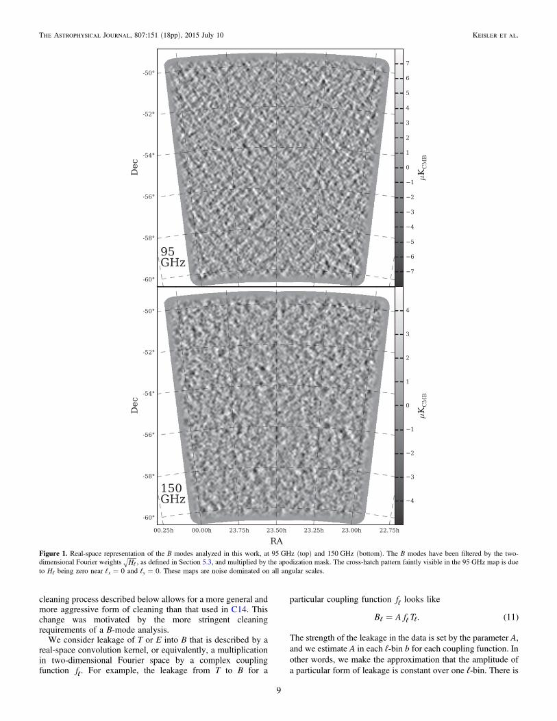
mn has been defined to optimizesensitivity to the lensed BB spectrum, we simply use the sameweight for the other CMB field combinations (EB, EE, etc.), asthe BB spectrum is the focus of interest for this work. InFigure 1 we show the real-space representation of the B modesanalyzed in this work, namely,B H BRe{ { }}ℓ ℓ

m mm m1= - .Each map Bm has been multiplied by the apodization mask for the purpose of visualization.

5.4. Convolutional Cleaning

Given that the CMB temperature and E-mode polarizationsignals are expected to contain significantly more power thanthe B-mode polarization signal, the potential for leakage from Tor E into B is a central issue for any BB analysis. The leakagefrom a number of instrumental effects—gain mismatch,differential pointing, differential beam ellipticity, incorrectpolarization angles, crosstalk, etc.—appears (to first order) as aspatially local leakage of the T or E skies into B. In otherwords, the leakage appears as a convolution of T or E into B.Here we describe a process, “convolutional cleaning,” bywhich we reduce the impact of convolutional T E B( , ) leakage. The basic idea is to use the CMB T and E modesthemselves to estimate and project out convolutional leakagefor O(100) convolution kernels per spectral band. Afterapplying this cleaning, we are largely insensitive to anypotential parity-violating cosmological TB or EB signal.We note that the cleaning process described here is similar to

a number of other techniques used to clean convolutional T andE leakage. For example, a global polarization angle offsetcauses convolutional E B leakage, and a number of recentworks (BICEP2 Collaboration 2014; POLARBEAR Collabora-tion 2014a; Naess et al. 2014; Keck Array & BICEP2Collaborations et al. 2015) use the EB spectrum, and to alesser degree the TB spectrum, to fit for (and in some casescorrect for) this offset. This technique fits the one-dimensionalEB spectrum to a single parameter, the polarization angleoffset. Another technique, “deprojection” (BICEP2 Collabora-tion 2014; Keck Array & BICEP2 Collaborations et al. 2015),cleans any potential convolutional T B leakage caused bydifferential gain, differential pointing, or differential beamellipticity. This technique takes advantage of the well-measuredtemperature skyand is performed on a per-detector-pair basisin the time-ordered data. Finally, a previous SPTpol analysis(C14) measured and corrected for convolutional T Q U( , )leakage using TQ and TU spectraand corrected the TE and EEspectra for the additional effects of crosstalk. The convolutional

8


cleaning process described below allows for a more general andmore aggressive form of cleaning than that used in C14. Thischange was motivated by the more stringent cleaningrequirements of a B-mode analysis.

We consider leakage of T or E into B that is described by areal-space convolution kernel, or equivalently, a multiplicationin two-dimensional Fourier space by a complex couplingfunction fℓ. For example, the leakage from T to B for a

particular coupling function fℓ looks like

B A f T . (11)ℓ ℓ ℓ=

The strength of the leakage in the data is set by the parameter A,and we estimate A in each ℓ-bin b for each coupling function. Inother words, we make the approximation that the amplitude ofa particular form of leakage is constant over one ℓ-bin. There is

Figure 1. Real-space representation of the B modes analyzed in this work, at 95 GHz (top) and 150 GHz (bottom). The B modes have been filtered by the two-dimensional Fourier weights Hℓ , as defined in Section 5.3, and multiplied by the apodization mask. The cross-hatch pattern faintly visible in the 95 GHz map is dueto Hℓ being zero near ℓ 0x = and ℓy = 0. These maps are noisedominated on all angular scales.

9


still freedom for ℓ-dependence of the leakage because theamplitude is allowed to vary between ℓ-bins.

We use coupling functions of the form

( )f k icos (12)ℓ ℓk kf q= +q

where k is a small integer k k{0, 1, , }maxÎ ¼ , ℓf is theazimuthal angle in two-dimensional Fourier space,

{0, 2}q pÎ , and the i k factor ensures that f corresponds to apurely real (rather than imaginary) real-space kernel. We usethis form because the coupling functions for well-known typesof leakage can be expressed as linear combinations ofcouplings with the form described above. For example,differential gain has a TB coupling f cos(2 )ℓ ℓfµ , differential

pointing has a TB coupling ( )f iℓ cos( ) cos(3 )ℓ ℓ ℓf fµ + , anda global polarization angle offset has an EB coupling f 1ℓ µ .We emphasize that we do not assume a particular physicalmechanism (such as differential pointing or differentialellipticity) for this leakage. Rather, we assume that the leakageis varying slowly in ℓand has an azimuthal dependencedescribed by kcos( )ℓf q+ for small integer k. We usek 4max = , which allows for the cleaning of any of the typesof leakage described above. We find that the main result of thiswork, the constraint on the amplitude of lensing B-modepower, is insensitive to the particular choice of kmax; the lensingamplitude shifts by ∼0.1σ when trying k {2, 4, 6}max Î .Conversely, we find that convolutional cleaning is an importantstep in this analysis. In the absence of convolutional cleaning,the nominal estimate of the lensing amplitude shifts signifi-cantly upward, by ∼3σ. This shift is driven mainly by changesin the first two bins of the 150 GHz × 150 GHz BB spectrum,which contain most of the sensitivity to lensing B modes.

The linear estimate of the amplitude A of a particular form ofleakage fℓ

kq in ℓ-bin b of the data Bℓm for spectral band m is

{ }( )A

B X f H

X f H

ˆRe *

(13)ℓ ℓ ℓ ℓ

ℓ ℓ ℓ

bk Xm ℓ b

m k mm

ℓ bk mm2

å

å=

q

q

q

Î

Î

where X T E{ , }Î and the weight Hℓmm is defined in

Section 5.3. The numerator is linear in the data Bℓm, and the

denominator is used to normalize the estimate. Because the150 GHz data are deeper than the 95 GHz data, we use the150 GHz Tℓ and Eℓ modes to estimate the leakage in the 95 and150 GHz Bℓ modes. We use a cross-spectrum approach to

estimate both B X fRe{( )* }ℓ ℓ ℓm kq and X fℓ ℓ

k 2q∣ ∣ . For our baselinevalue of k 4max = , there are a total of 18 leakage modes per ℓ-bin, or 90 modes for all five ℓ-bins, per spectral band.

Ideally, we would use these estimates of the leakageamplitudes to remove from the data Bℓ

m the inferred leakedBmode,

B A X f qˆ (14)ℓ ℓ ℓ ℓm

k Xbbk Xm k

bleak, å=

q

q q

where the two-dimensional binning operator q ℓb is one forℓ bÎ and zero otherwise. In practice, however, as a result ofthe non-orthogonality of the different modes being removed,the cleaning process does not converge after one iteration. We

address this issue using a damped, iterative scheme. In eachiteration we estimate the amplitude of each form of leakage;subtract a damped version of the inferred leaked mode,

B0.2 ℓmleak, , from Bℓ

m; and repeat for all forms of leakage. Weiterate over these steps 20 times, at which point the process hasconverged. We use the accumulated estimate for each leakageamplitude to construct the final inferred leakage mode, Bℓ

mleak, .

Finally, we subtract Bℓmleak, from Bℓ

m i, for each bundle i. To be

clear, the same Bℓmleak, is subtracted from all bundles. In other

words, all two-dimensional Bℓ that appear in this work havebeen cleaned in this way, with one exception: the Fourierweights Hℓ are calculated using Bℓ that have not been cleaned.We find that the convolutional cleaning process strongly

suppresses a form of convolutional leakage that we expect to bepresent in the SPTpol data: crosstalk-induced leakage. We haveused our simulated maps to determine that convolutionalcleaning reduces the additive bias to the BB spectrumintroduced by crosstalk by factors of ∼20–100. The cost ofthis improvement, however, is the introduction of a small,additive noise bias, as discussed below in Section 5.5.1 and inthe appendix.

5.5. Unbiased Spectra

Here we describe the process by which the raw BBbandpowers described in Section 5.3 are processed intounbiased bandpowers. The raw bandpowers are subject toadditive and multiplicative biases, and we correct for thesebiases using simulated bandpowers.

5.5.1. Additive Bias

Our strategy for dealing with additive bias—any BB powerthat is present in the absence of a true B-mode polarizationsignal—is straightforward. We measure the mean BB powerpresent in noisy, simulated bandpowers generated using TEinput skies (i.e., no true BB power), and we subtract this biasfrom the data bandpowers and the simulated TEB bandpowers.This subtraction is performed prior to correcting for anymultiplicative bias. The additive biases can to some degree beorganized as follows.

1. E B from geometry and filtering—imperfect separa-tion of E and B on a small area of sky and the high-passfiltering of the time-ordered data result in E B leakage.The resulting bias in BB is approximately +0.6σ in thelowest ℓ-bin of the 150 × 150 spectrum, and smaller than0.1σ in other ℓ-bins of this spectrum or any ℓ-bin of theother spectra.

2. T E B( , ) from crosstalk—the electrical crosstalkbetween detectors results in T E B( , ) leakage, pre-dominantly T B . Although the raw crosstalk-inducedadditive bias is as high as 1.0σ in the lowest ℓ-bin of150 × 150, convolutional cleaning reduces this to 0.1s< .

3. Negative noise bias from convolutional cleaning—wefind that the convolutional cleaning step introduces anegative bias. By analyzing two sets of simulations thathave convolutional cleaning turned on and off, we canisolate this effect. We find that its magnitude and shapeare in broad agreement with a simplified analyticcalculation given in the appendix. The amplitude of thebias is approximately −0.4σ in the lowest two ℓ-bins of

10


the 95 × 95 and 150 × 150 spectra, smaller elsewhere, andapproximately zero at 95 × 150. The convolutionalcleaning process has strongly attenuated biases arisingfrom convolutional leakage (crosstalk, beam systematics,etc.) in exchange for a small noise bias that we cancharacterize effectively perfectly.

The additive biases are shown in Figure 2. We subtract thesebiases from the measured spectra, and we address systematicuncertainties associated with the additive biases in Section 5.9.

5.5.2. Multiplicative Bias

After removing the additive bias, we correct for themultiplicative bias. The bandpowers Cb

are a biased estimateof the true binned sky power, Cb¢, due to effects such as time-ordered data filtering, beam smoothing, finite sky coverage, andmode-mode mixing from the source and apodization mask. Thebiased and unbiased estimates are related by

C K C (15)bB B

bbB B

bB B

m n m n m nº ¢ ¢

where the K matrix accounts for the effects of the instrumentalbeam and time-ordered data filtering and the application of theapodization mask (). K can be expanded as

( )K P M F Q[ ] . (16)bb bℓ ℓℓ ℓ ℓ b=¢ ¢ ¢ ¢ ¢where Fℓ is the effective transfer function from the beam andthe filtering of the time-ordered data, Pbℓ is the binningoperator, andQℓ b¢ ¢ its reciprocal (Hivon et al. 2002). The mode-coupling kernel M [ ]ℓℓ¢ accounts for the mixing of powerbetween bins due to the apodization mask. The mode-couplingkernel is calculated analytically, as described in the Appendixof C14. The calculation corrects only for B B coupling andeffectively assumes that there is no E B coupling. The latteris,of course, not true, but we correct for E B leakage bysubtracting off an additive bias, as described in Section 5.5.1.As in C14, the effective transfer function Fℓ is calculated bycomparing the mean simulated spectra to the theory spectrum

input to the simulations. The calculation is iterative andconverges after two iterations.

5.6. Bandpower Covariance

We approximate the covariance between BB bandpowers ascompletely diagonal, and we take the variance of bandpowersfrom the set of 200 noisy simulations as our estimate of thediagonal variances. There are two sets of covariances: thosethat use TE input skies and thus naturally account for the noisevariance and the variance from T and E leakage, and those thatuse TEB input skies, which additionally account for variancefrom true BB power. The TE variances are useful for rejectingthe C 0BB = hypothesis. The TEB variances are only slightlylarger than the TE variances, at most 20% larger, implying thatnoise power dominates over signal power, as expected.We have used the noisy simulated bandpowers to assess the

validity of the diagonal covariance approximation. Weattempted to measure the covariance between off-diagonalspectral combinations, e.g., (95 GHz × 95 GHz) and (95 GHz ×150 GHz), or between neighboring ℓ-bins. In each case, thedistribution of covariance estimates is consistent with zero.This is not surprising given that the covariance is dominated bynoise power and the noise is expected to be uncorrelatedbetween spectral bands and between ℓ-bins. We have alsoexplicitly tested the importance of the off-diagonal covarianceterms at (95×95)×(95×150) and (150×150) ×(95×150). We estimated these terms using an analyticapproximation, altered the covariance matrix accordingly, andfound that the main result of this work, the constraint on theamplitude of lensing B-mode power, changed by ∼0.1σ. Forsimplicity, we do not include these off-diagonal terms.We note that our simulation input skies contain Gaussian

realizations of lensed BB power and therefore do not accountfor the ∼20% inter-ℓ-bin correlation present for non-Gaussian,truly lensed B modes (Benoit-Lévy et al. 2012). Given that thenon-Gaussian structure leads to a 20% bin-bin correlation on asource of power (lensed BB power) that itself contributes only10%–20% of the bandpower variance, we ignore the non-Gaussian contribution in our TEB variances.Finally, we note that, because our simulations were free of

foreground power, we have slightly underestimated the BBvariance. Power from randomly distributed, polarized pointsources should be negligible; even the upper limits of thePoisson powers considered in Section 6 are <1% of the datanoise power. Variance from polarized galactic dust should alsobe small compared to the noise power. For our nominal dustmodel described in Section 6.1, the dust power is approxi-mately 1% of the noise power in the lowest ℓ-bin of the150 GHz × 150 GHz spectrum, and smaller elsewhere.

5.7. Bandpower Window Functions

We compute bandpower window functions to allow themeasured bandpowers to be compared to theoretical powerspectra. The window functions, w ℓℓ

b , are defined through therelation

( )C w ℓ C . (17)b ℓb

ℓ=

Figure 2. Thick solid lines show the net additive bias to the three BB spectra asa fraction of the diagonal statistical uncertainty. Both of these quantities aredetermined using noisy simulated data. The dashed lines show the contributionto the bias from geometry and filtering, the dotted lines show the contributionfrom residual crosstalk, and the dot-dashed lines show the contribution fromthe convolutional cleaning process. The net biases are 0.5s< and are subtractedfrom the measured spectra.

11


Following the formalism described previously in Section 5.5.2,this can be rewritten as

( )C K P M F C , (18)bbb

b ℓ ℓ ℓ ℓ ℓ1= -

¢ ¢ ¢ ¢

which implies that

( )w ℓ K P M F . (19)ℓb

bbb ℓ ℓ ℓ ℓ

1= -¢ ¢ ¢ ¢

5.8. Null Tests

In this section we test the internal consistency of the data byconsidering two types of null tests. First, we consider the TBand EB spectra. Second, we consider a suite of “jackknife” teststhat are sensitive to potential instrumental systematics.

5.8.1. TB and EB Spectra

Although we are interested primarily in the BB powerspectrum, here we consider the other spectra that contain the B-mode polarization field, namely, the TB and EB spectra. We donot expect a cosmological signal in these spectra.

Typically one would compare the TB and EB data spectra tothe null hypothesis, namely C C 0TB EB= = . Here, due to theadded complexity of the convolutional cleaning step, we do notnecessarily expect the simulated TB and EB spectra to havezero mean, and indeed we find that several of the simulatedbandpowers have negative mean values. Nevertheless, we cantest whether the data spectra are consistent with the distributionof simulated spectra. We find that the TB and EB data spectra at95 × 95, 95 × 150, and 150 × 95 are all consistent with thedistribution of simulations. However, the TB and EB dataspectra at 150 × 150 are systematically lower than the mean ofthe simulated spectra. TB is low by [−2.3, −2.1, −1.8, −1.4,−1.4]σ in the different ℓ-bins, while EB is low by [−1.5, −1.5,−3.0, −0.6, −1.5]σ.

While we cannot offer an explanation for this differencebetween the data and the simulations, we argue that it is notsignificant for the main focus of this work, the BB spectrum.More specifically, we use the difference between the data andsimulation spectra to estimate the resulting spurious BB, andfind that it is small compared to our statistical uncertainties. Forexample, for TB the difference between the data andsimulations is C C Cb

TBbTB

bTB,data ,simsd º - á ñ, and the estimate

of the associated spurious BB power is C C C( )bBB

bTB

bTT2d= .

We find the spurious BB estimated from either TB or EB to bevery small, less than 0.2% of the expected ΛCDM lensed BBspectrum.

We note that a number of recent B-mode studies (BICEP2Collaboration 2014; POLARBEAR Collaboration 2014a;Naess et al. 2014; Keck Array & BICEP2 Collaborationset al. 2015) use the EB spectrum, and to a lesser degree the TBspectrum, to fit for a global polarization angle offset. In some ofthese studies, the derived polarization angle offset (typically oforder 1°) is inconsistent with zero and is used to correct thepolarized maps. The EB spectra are consistent with zero afterapplying this correction, and in all cases, the authors find thatthis correction makes little difference to the BB signal ofinterest.

The convolutional cleaning process that we employ in thiswork is similar to this technique. In the language ofconvolutional cleaning, we have reduced our sensitivity to aglobal polarization angle offset by projecting out the

azimuthally independent (k= 0) component of the two-dimensional EB spectrum. The convolutional cleaning processalso simultaneously projects out higher-order (higher k) modes.The net result is that convolution cleaning forces the EBspectrum to be close to zero. For example, the anomalouslynegative 150 × 150 EB spectrum described above is equivalentto an effective global polarization angle offset of only 0 ◦. 02.

5.8.2. Jackknives

We perform a suite of “jackknife” tests to further validate theconsistency of the data. In each jackknife test the bundle mapsare sorted according to a metric designed to trace a potentialsystematic effect, and “jackknife maps” are constructed bydifferencing high-metric bundle maps with low-metric bundlemaps. The resulting jackknife maps should not contain skysignal and should have a power spectrum, the jackknifespectrum, consistent with noise. We construct the jackknifespectrum by taking the mean cross-spectrum among thejackknife bundle maps. We note that we do not apply theconvolutional cleaning step to the bundle maps going into thejackknife maps. The convolutional cleaning step would have noeffect, as it would remove the same modes identically fromeach of the maps prior to taking their difference.We perform four jackknife tests.

1. Left–Right: Jackknife maps are made by differencingdata from left-going and right-going scans. This tests forany power or systematic effect that is present morestrongly in one scan direction, such as spurious powercaused by the step in telescope elevation at the end ofeach left–right scan pair.

2. Ground: Jackknife maps are made by dividing the mapsinto two subsets thought to have different susceptibility toground contamination. We use the same azimuthal rangemetric used in SPT-SZ power spectrum analyses such asShirokoff et al. (2011). This tests for spurious powerfrom nearby buildings or other sources of contaminationthat are fixed to the ground.

3. 1st half–2nd half: Jackknife maps are made by differen-cing data from the first and second halves of the set ofchronologically ordered map bundles. This tests for anysystematic associated with the changes made to theSPTpol receiver between 2012 and 2013, systematicsassociated with small changes to the scan strategy madein late 2012, or any other slowly varying systematic.

4. Visual Inspection: Jackknife maps are made by differen-cing map bundles that show visually identified anomalies(e.g., faint stripes or spots) and those that do not. Thistests for systematic power associated with these features.

We use a slightly different notation for the jackknifebandpowers than is used for the main bandpowers. Eachjackknife bandpower is Cfsj

b , where f BB EB TB{ , , }Î denotesa CMB field combination, s {Î 95 × 95, 95 × 150, 150 × 150}denotes a spectral combination, and j {LR, GROUND,ÎTIME, VIS} denotes a jackknife.

We test the consistency of the jackknife spectra with the nullhypothesis as follows. We estimate the diagonal covarianceof the jackknife bandpowers, ( )Cb

fsj2s , using the varianceamong the cross-spectra divided by the number of unique

12


cross-spectra. Next, we define jackknife “χ bandpowers,”

( )C

C(20)b

fsj bfsj

bfsj

cs

º

and calculate four test statistics to determine the compatibilityof this set of spectra with the null hypothesis. These teststatistics are:

1. ( )max fsj b bfsjcå∣ ∣ —this tests for spectra that are prefer-

entially positive or negative across the full multipolerange;

2. ( )max ( )fsj b bfsj 2cå —this tests for spectra that preferen-

tially have outlying bandpowers;3. ( )max ( )bfsj b

fsj 2c —this tests for any particularly strongoutlying bandpower;

4. ( )bfsj bfsj 2å c —this tests for a general tendency to have

outlying bandpowers.

We compare the data values of these test statistics to thoseobtained using a set of 10,000 zero-mean, unit-width Gaussianrealizations of each b

fsjc . We calculate the probability to exceed(PTE) the value of each data test statistic given the values inthe set of simulated test statistics. Finally, we define a globaltest statistic, Pjoint, the probability to simultaneously exceed allof the test statistics, and calculate the probability to exceed

P1 joint- , again using simulations.As the focus of this work is the BB spectrum, our nominal set

of jackknife CMB field combinations is simply BB{ }. We findthat the PTEs for the four test statistics are 0.29, 0.60, 0.15, and0.09, and the global PTE is 0.22. We take this as evidence thatthe BB spectra do not have significant contamination underthese jackknife tests.

We have also repeated these jackknife tests using anexpanded set of CMB field combinations, BB EB TB{ , , }.Owing to the high signal-to-noise imaging of T and E modes,these tests are in principle more difficult to pass. In this case,the PTEs for the four test statistics are 0.41, 0.59, 0.39, and0.02, and the global PTE is 0.14. We take this as furtherevidence that the B-mode data used in this work donot havesignificant contamination under these jackknife tests.

5.9. Systematic Uncertainties

Here we discuss several potential sources of systematicuncertainty in the BB power spectrum measurement. In allcases we demonstrate that the systematic uncertainty is muchsmaller than the statistical uncertainties and can be safelyignored.

5.9.1. Uncertainty in Additive BB Bias

As described in Section 5.5.1, we use simulations todetermine the additive biases that must be subtracted fromthe measured BB bandpowers. Here we assess the accuracywith which we have determined these biases.

First, we consider the uncertainty due to using a finitenumber of simulation realizations. We have used 200realizations, leading to uncertainties on the mean biases of0.07σ per ℓ-bin.

Next, we specifically consider T B leakage, which isdominated by crosstalk leakage. While the raw bias is as highas 1.0σ in the lowest ℓ-bin of 150 × 150, convolutional cleaning

reduces this bias to at most 0.1σ per ℓ-bin. The uncertainty inthe absolute temperature calibration is less than 3% in power,resulting in a negligible 0.003σ uncertainty in the additive bias.Similarly, the underlying ΛCDM TT spectrum is constrained toapproximately the same level of precision, and its uncertaintycan be safely ignored.Next, we consider E B leakage, which is caused primarily

by the field geometry and the filtering of time-ordered data.This leakage results in a bias as high as 0.6σ. The uncertainty inthe absolute polarization calibration is less than 5% in power,resulting in a negligible 0.03σ uncertainty in the additive bias.Again, the underlying ΛCDM EE spectrum is constrained to asimilar level of precision.Finally, we consider the negative noise bias from convolu-

tional cleaning. This bias is approximately −0.4σ per ℓ-bin inthe 95 × 95 or 150 × 150 spectra. However, because we use thedata to generate the noise realizations used in the simulations,there is essentially zero systematic uncertainty in the level ofthis bias.

5.9.2. Uncertainty in Multiplicative Bias in BB

We discussed above how the uncertainty in the absolutepolarization calibration results in a (negligible) uncertainty inthe additive BB bias from E B . It also results in anuncertainty on the amplitude of the measured BB spectrum. Theuncertainty is 3% and 4% in power for the 150 × 150 and95 × 150 spectra, respectively, where nearly all of oursensitivity lies. This results in a ∼0.1σ global systematicuncertainty on the amplitude of the BB spectrum. We note thatthis small uncertainty does not affect the significance withwhich we detect BB power, as the statistical uncertainties arenoisedominated, and the noise would suffer from the samemiscalibration.

5.9.3. T Q U Leakage

We see evidence for 0.65% ± 0.15% leakage of T into Q andU at 150 GHz. We measure this using TQ and TU spectra asdescribed in C14. The source of this leakage is not known,although it could arise from our celestial calibration source,RCW38, being ∼0.5% polarized. Unlike previous SPTpolanalyses that explicitly cleaned this leakage from the Q and Umaps, this work relies on convolutional cleaning to remove thisleakage. We expect the convolutional cleaning process toreduce the associated additive BB bias by at least a factor of 20,resulting in a bias that is at most ∼0.15σ in the lowest ℓ-bin of150 × 150 and smaller elsewhere. The leakage is smaller yet at95 GHz.

5.9.4. Effect of Crosstalk on Beams

Because the electrical crosstalk between detectors happens tobe preferentially negative, the array-averaged temperaturebeam will tend to lose solid angle. The array-averagedpolarization (Q/U) beams, on the other hand, will not losesolid angle, owing to partial cancellation of crosstalk from setsof nearly randomly oriented detectors. This results in the array-averaged temperature and polarization beams differing slightly.Throughout this work we have used the effective temperaturebeam as measured with observations of planets and activegalactic nuclei (AGNs). This implies that our polarized powerspectra have been debiased using slightly incorrect beamfunctions, and that our simulations were performed using

13


slightly incorrect beams. The ratio of the effective temperatureand polarization beam functions can be broken down into an ℓ-independent mean offset and an ℓ-dependent shape around thatmean offset. The ℓ-independent offset is naturally accounted forwhen we calibrate our TT and EE spectra independently. The ℓ-dependent shape is not accounted for, but is well approximatedby a linear tilt from +2% to −2% in power across the ℓ range ofthis work. This results in negligible ( 0.1s< ) systematicuncertainties in the removal of additive and multiplicative BBbiases.

5.9.5. Time-dependent Crosstalk

In our baseline simulations, the crosstalk matrix Vab thatencodes the coupling between detectors a and b was fixed. Infact, we have evidence that there is some amount oftimevariation in the crosstalk matrix. Time-varying crosstalkcould potentially introduce a different level of additive bias inthe BB spectrum than time-independent crosstalk does. Wehave addressed this issue with a second set of simulations inwhich the crosstalk matrix Vab was allowed to vary, perobservation, in a way that mimics the timevariation weobserve. We find that the resulting additive BB bias is slightlysmaller than in the time-independent case. The difference is0.2σ in the lowest ℓ-bin of the 150 × 150 spectrum, and smallerthan 0.04σ in all other ℓ-bins.

5.9.6. Small-scale Beam Features

We have used observations of Venus to measure the array-averaged beams on small scales (r 3< ¢). The resultingpolarization maps can be used to place upper limits on theT B leakage due to anomalous beam features on these smallscales. We estimate the spurious BB power asC C C( ) 20.ℓ ℓ

TB TTℓTT,Venus ,Venus 2 , CDML We have scaled the

ΛCDM TT spectrum by the appropriate beam factor and havedivided by 20, the minimum level of improvement thatconvolutional cleaning provides on simulated crosstalk-induced leakage (a stand-in for other types of convolutionalleakage). We find that the resulting spurious BB wouldintroduce a net bias less than 0.02σ.

While the Venus maps provide an upper limit on the T Bleakage from small-scale beam features, they do not addressE B leakage. However, given that the limits on T B areso small, and given that EE is a factor of ∼50 smaller than TT atthese multipoles, we do not expect E B from small-scalebeam features to be significant.

5.9.7. Large-scale Beam Features

We use observations of the Moon to estimate thatapproximately 5% of the beam solid angle is contained in theradial range r3 25¢ < < ¢. If we consider a pessimistic scenarioin which this portion of the beam, when averaged over alldetectors, couples T B with 5% efficiency or E B with50% efficiency (both in map units), and that convolutionalcleaning reduces the resulting BB power by a factor of 20, theresidual BB power is less than 0.03σ for all ℓ-bins.

5.9.8. Systematics Summary

To summarize, we have considered a number of systematicuncertainties and demonstrated that they are small compared tothe statistical uncertainties. When added in quadrature with the

statistical uncertainties, the systematic uncertainties associatedwith additive biases would increase our total uncertainty by∼3% in the lowest ℓ-bin of the 150 × 150 spectrumand wouldhave a smaller effect elsewhere. The systematic uncertainty inthe global multiplicative bias is ∼3.5%. As discussed inSection 6, this is significantly smaller than the ∼20% precisionwith which we measure any BB signal. Additionally, thismultiplicative uncertainty does not affect the significance withwhich we detect a BB signal, as it would affect the bandpowersand their uncertainties nearly equally.

5.10. Bandpowers

The final BB bandpowers are provided in Table 1 and shownin Figure 3. The bottom panel of Figure 3 shows the inverse-variance-weighted combination of the three sets of band-powers. The spectrally combined bandpowers are for visualiza-tion purposes only; the likelihood employed in Section 6 usesthe original set of three bandpowers. The bandpowers,covariance matrix, and bandpower window functions areavailable at the SPT Web site.39

6. INTERPRETATION

6.1. Significance of BB Lensing Measurement

The bandpowers from this work shown in Figure 3 show aclear preference for non-zero (positive) power. Using amultivariate Gaussian likelihood and the bandpower covariancematrix defined in Section 5.6, we find that the χ2 of the data tothe null hypothesis of zero BB power is 41.5, with an associatedPTE for 15 degrees of freedom (dof) of 3 10 4´ - . The data arenot well fit by zero sky power. A far better fit is the predictedlensing BB spectrum from (for instance) the PLANCK+LENS best-fit model from Table II of Planck Collaboration XVI (2014).With zero free parameters, the χ2 of our data to this model is18.1 for 15 dof, for a PTE of 0.25, and a 2cD relative to zeroBB power of 23.4.To translate this preference into a detection significance, we

introduce a single parameter, Alens, which we use to artificiallyscale the predicted lensing BB power from our fiducialcosmological model. We explore this parameter space (andall parameter spaces discussed subsequently in this work) usingthe Markov chain Monte Carlo method provided by theCosmoMC40 software package (Lewis & Bridle 2002). The χ2

for the best-fit model is 17.6 (PTE 0.23= ). The data prefer theaddition of this single parameter by a 2cD value of 23.9,translating to a 4.9σ detection of lensing, under the assumptionof no other sky components. Note that all of these χ2 values arecalculated with noise variance only (i.e., no sample variancefrom sky signals), because we are only asking at what level thedata in this patch of sky prefer a component that looks likelensed B modes, and are not attempting to relate the amplitudeof this component to any global cosmological parameter.We do expect other sky components to contribute to the

measured BB power, so we also fit for the amplitude of thelensing B modes in the presence of other signals. We know thatthere will be contributions from polarized emission fromextragalactic sources and from dust emission within our ownGalaxy, and we add parameters to the fit describing each ofthese.

39 http://pole.uchicago.edu/public/data/keisler15/40 http://cosmologist.info/cosmomc/

14


http://pole.uchicago.edu/public/data/keisler15/

http://cosmologist.info/cosmomc/

The area of sky used in this work is contained within theBICEP2 areaand should thus have a similar level of galacticpolarized dust emission. Motivated by the recent Planck results(Planck Collaboration et al. 2014a), we model the contributionfrom Galactic dust as

Dℓ ℓ

C

A DS S

S

ℓ

( )( 1)

2( )

( )( ) ( )

( ) 80(21)

ℓ ℓdust

1 2dust

1 2

dust 80dust

0 0dust 1 dust 2

dust2

0

0.42

n np

n n

n nn n

n

´ º+

´

= ´æèççç

öø÷÷÷

-

where C ( )ℓdust

1 2n n´ is the contribution of dust to the95 GHz × 95 GHz, 95 GHz × 150 GHz, or 150 GHz × 150 GHzspectrum; Adust is an overall scaling of the amplitude of thedust power spectrum at all frequencies; 150 GHz0n = ;

D ( )80dust

0 0n n´ is the best-fit value of the dust BB spectrum

in the BICEP2 observing region at 150 GHz and ℓ = 80,according to Planck Collaboration et al. (2014); and Sdust is thePlanck Collaboration et al. (2014) assumption for the spectralbehavior of the dust (in units of CMB temperature). Weintegrate the dust spectrum over the measured SPTpolbandpasses. The only free parameter in our fit to this model isAdust. For reference, the nominal value of Adust = 1 corresponds

to powers of D80dust= (0.00169, 0.00447, 0.0118) K2m in the

SPTpol spectra at (95 × 95, 95 × 150, and 150 × 150).We model the contribution from extragalactic sources as a

C constantℓ = term, as would be expected if the emission wasdominated by the Poisson noise in the number of sources in ourobserving region, rather than the angular clustering of thosesources. We allow the amplitude of the Poisson term in ourthree frequency combinations to vary independently, giving usthree free parameters, APS,95 95´ , APS,95 150´ , and APS,150 150´ .Based on the arguments in BICEP2 Collaboration (2014)

and BICEP2/Keck & Planck Collaborations et al. (2015), weexpect the contribution from Galactic synchrotron emission tobe far below our ability to detect it, and we ignore thiscontribution in our analysis. We also ignore the contributionfrom the polarized emission by clustered extragalactic sources.We expect this signal to be far less important relative to thePoisson signal in polarization measurements than it is intemperature measurements, because the clustered signal isdominated by dusty, star-forming galaxies (DSFGs), which weexpect to have a much smaller polarization fraction than thesynchrotron-emitting AGNsexpected to contribute the bulk ofthe Poisson signal (e.g., Seiffert et al. 2007; Battye et al. 2011).Finally, we add a component to our fit that has the shape of

the expected IGW B-mode signal, and we use the freeparameter r to control the amplitude of this component. Wedo not expect to be able to distinguish this component fromGalactic dust in the ℓ range and sensitivity level in this work;we include the IGW component primarily to facilitate directcomparison between our lensing results and those fromBICEP2 (see Section 6.2 below).Our nominal fit includes priors on all five nuisance

parameters (APS,95 95´ , APS,95 150´ , APS,150 150´ , Adust, and r).The nominal prior on Adust is a Gaussian centered on 1.0, with

0.3s = . The nominal priors on Poisson power are uniformbetween zero and four times the value calculated for eachparameter by integrating source models (De Zotti et al. 2010for AGNs;Negrello et al. 2007 for DSFGs) up to theunpolarized flux cut of 50 mJy and assuming polarizationfractions of 5% for AGNs and 2% for DSFGs (the upperbounds from Seiffert et al. 2007 and Battye et al. 2011,respectively). For reference, the upper edges of Poisson

Table 1BB Bandpowers, ℓ Cℓcenter (10 3m- K2)

95 × 95 95 × 150 150 × 150 Combined

ℓcenter ℓ Range ℓCℓ ℓC( )ℓs ℓCℓ ℓC( )ℓs ℓCℓ ℓC( )ℓs ℓCℓ ℓC( )ℓs

500 300–700 3.4 1.4 0.88 0.55 0.57 0.33 0.76 0.28900 700–1100 2.9 1.1 1.18 0.50 0.51 0.32 0.82 0.261300 1100–1500 0.4 1.3 0.27 0.50 1.07 0.37 0.77 0.291700 1500–1900 0.2 1.5 −0.23 0.55 0.16 0.38 0.04 0.302100 1900–2300 −1.7 1.6 −0.59 0.61 −0.29 0.47 −0.47 0.36

Note. BB bandpowers and uncertainties measured in this work. The last two columns give results for the inverse-variance-weighted combination of the three sets ofbandpowers.

Figure 3. Top: BB power spectrum bandpowers from the individual95 GHz × 95 GHz, 95 GHz × 150 GHz, and 150 GHz × 150 GHz spectra.Bottom: inverse-variance-weighted combination of the three sets of band-powers in the top panel. For reference, the expected lensed BB spectrum fromthe PLANCK+LENSING+WP+HIGHL best-fit model in Table 5 of PlanckCollaboration XVI (2014) is shown by a solid gray line in each plot.

15


Cℓ priors are 1.9 10 K7 2m´ - , 9.1 10 K8 2m´ - , and 4.4 ´10 K8 2m- at 95 × 95, 95 × 150, and 150 × 150, respectively.The prior on r is uniform between 0 and 0.4. We also place aprior on Alens (uniform between 0 and 3.0), but the posterior onAlens in all fits is dominated by the data, not the prior.The best-fit point in this nominal six-parameter space

(including priors) has a χ2 value of 17.9. If we fix A 0lens =and re-fit, the best-fit point has a χ2 value of 36.8. Thus, thedata show a preference of 18.92cD = , or 4.3σ, for lensing Bmodes when we marginalize over foreground parameters.

6.2. Best-fit Lensing Amplitude and Comparisonwith Previous Results

To report a value of Alens that can be used to assess thevalidity of the assumed cosmological model and to compare toother values in the literature, we repeat the six-parameter fitincluding BB sample variance in the uncertainty budget. Thebest-fit value and 1s uncertainty from this fit are

A 1.08 0.26 (22)lens =

consistent with the value of 1.0 that we would expect if thecosmological model we assumed were correct. The constrainton Alens is not strongly dependent on the foreground priors: ifwe increase the upper limit of the Poisson priors to 100 timesthe nominal power, the best-fit value of Alens shifts by less than1σ, and the error bar increases by less than 10%. Similarbehavior is seen when the Adust prior is changed to a uniformprior between 0 and 3.

Figure 4 demonstrates that the measurement of BB power inthis work is at least visually consistent with previousmeasurements in the same ℓ range. The most straightforwardway to compare the results quantitatively is to use the reportedconstraints on Alens. This comparison is complicated somewhatby the fact that these values are in general reported with respectto BB spectra predicted using different values of cosmological

parameters. The differences between the predicted amplitudesare typically much smaller than the 1σ uncertainty on Alensfrom any of the measurements, however, and we will ignorethem in the following comparison.First, we compare to other B-mode power spectrum

measurements. The best-fit value of Alens from POLARBEARmeasurements of the B-mode power spectrum was 1.12 ± 0.61(statistical only, POLARBEAR Collaboration 2014a), consis-tent with the value we find here. The ACTPol collaborationdoes not report a value of Alens from their B-mode powerspectrum (Naess et al. 2014). BICEP2 Collaboration (2014)reports a 5.5σ detection of lensed B modes and a best-fit valueof A 1.75lens , roughly 2σ above 1.0, with no marginalizationover foregrounds. We have used the publicly available BICEP2likelihood module41 to repeat this analysis with a margin-alization over foreground and IGW tensor power that mirrorsthe SPTpol analysis presented here. We obtain a constraintfrom the BICEP2 data of A 1.45 0.38lens = , roughly 1.2σabove 1.0. More recently, BICEP2/Keck & Planck Collabora-tions et al. (2015) reported a strong (7σ) detection of lensing Bmodes at ℓ 200~ : A 1.13 0.18lens = . This constraint wasobtained after marginalizing over contributions from IGWtensor power and polarized galactic dust emissionandrepresents the most precise direct measurement of lensing Bmodes to date. To summarize, these BB power spectrummeasurements are consistent with each otherand with theΛCDM prediction. These measurements suggest that the BBspectra in these particular fields and at these observingfrequencies are dominated by lensing B modes, at least atℓ 200 . The SPTpol BB spectrum presented here isparticularly useful in that regard, in the sense that A 2lens ⩾—a rough proxy for a scenario in which other sources of Bmodes dominate—is rejected at 3s> independent of whether ornot we marginalize over foregrounds.Next, we compare to measurements of the lensing B-mode

power spectrum that rely on cross-correlation with tracers ofthe CMB lensing potential ϕ. In these analyses, a lensing B-mode template is constructed by lensing measured E modes byan estimate of ϕ derived from CIB maps or CMB lensing. TheB-mode template is then correlated with the measured B modesto estimate the lensing BB power spectrum. The linearrelationship between the CIB and ϕ is, in turn, based on theCℓ

CIBf- spectrum measured by Planck, and it would thereforebe surprising if these CIB cross-correlation analyses gaveresults that were not consistent with the ϕϕ spectrum measuredby Planck (which itself is consistent with theΛCDM prediction). The best-fit value of Alens from the SPTpolCIB cross-correlation analysis in H13 was 1.092 ± 0.141. ThePOLARBEAR collaboration does not report a value of Alensfrom their CIB cross-correlation analysis. The ACTPolcollaboration measured A 1.30 0.40lens = in their cross-correlation analysis with PlanckCIB data (van Engelenet al. 2014). Planck Collaboration et al. (2015) also detectlensed B modes in this fashion and report best-fit values ofA 0.93 0.10lens = when using the CIB as a ϕ tracer orA 0.93 0.08lens = when using the quadratic-estimator-derived ϕ. These measurements are consistent with theΛCDM prediction and with our measured value.Finally, we note that our constraint on Alens is also consistent

with determinations of this parameter from quadratic-estimator

Figure 4. BB power spectrum measurements from SPTpol (this work),ACTpol (Naess et al. 2014), BICEP2/Keck (Keck Array & BICEP2Collaborations et al. 2015), and POLARBEAR (POLARBEARCollaboration 2014a). The highest multipole bin of the ACTpol data is notshown. The solid gray line shows the expected lensed BB spectrum from thePLANCK+LENSING+WP+HIGHL best-fit model in Table 5 of Planck CollaborationXVI (2014). The dotted line shows the nominal 150 GHz BB power spectrumof Galactic dust emission used in this work. This model is derived from ananalysis of polarized dust emission in the BICEP2/Keck field using Planck data(Planck Collaboration et al. 2014). The dot-dashed line shows the sum of thelensed BB power and dust BB power.

41 http://bicepkeck.org

16


http://bicepkeck.org

reconstructions of the lensing potential using the four-pointfunction of CMB temperature and polarization data. Thestrongest such constraint (Planck Collaboration et al. 2015)uses full-mission Planck data to yield A 0.983 0.025lens = .Additionally, three recent works use polarization-only quad-ratic estimators to constrain Alens. POLARBEAR Collaboration(2014c) findsA 1.06 0.47lens = (statistical only), Storyet al. (2014) use SPTpol data to measure Alens=0.92 0.25(statistical only) on the same 100 deg2

field used in this work,and Planck Collaboration et al. (2015) findA 1.252 0.350lens = . Again, these measurements of Alensare consistent with the ΛCDM prediction and with ourmeasured value.

7. CONCLUSION

We have presented a measurement of the B-mode powerspectrum (BB spectrum) using data from 100 deg2 of skyobserved with SPTpol in 2012 and early 2013. The BBspectrum is estimated in the multipole range ℓ300 2300< <for three spectral combinations: 95 GHz × 95 GHz, 95 GHz ×150 GHz, and 150 GHz × 150 GHz. These data provide the bestmeasurement of the B-mode power spectrum on these angularscales to date.

Several sources of bias—all at a level below the statisticaluncertainty in the power spectrum—are identified andsubtracted from the data. The resulting power spectrum isstrongly inconsistent with zero power but consistent withpredictions for the BB spectrum arising from the gravitationallensing of E-mode polarization. In a six-parameter fit thatincludes the predicted lensed B-mode spectrum scaled by asingle parameter Alens, as well as contributions from Galacticdust, extragalactic sources, and any IGW B-mode signal, wefind A 1.08 0.26lens = . The null hypothesis of no lensed Bmodes is ruled out at 4.3σ after marginalizing over foregroundparameters (4.9σ if foregrounds are fixed to zero).

Improved constraints on the BB spectrum are expected soonfrom a number of ongoing CMB experiments. For example, in2014 December SPTpol completed the second of three years ofobservation of a 500 deg2

field, and the resulting data willsignificantly improve on the BB spectrum presented in thiswork. A future generation of instruments aims to furtherconstrain inflationary B modes, provide maps of lensing Bmodes over large fractions of the sky, and constrain or measurethe mass in neutrinos. We can expect significant progress inthis field in the coming decade.

The South Pole Telescope program is supported by theNational Science Foundation through grant PLR-1248097.Partial support is also provided by the NSF Physics FrontierCenter grant PHY-0114422 to the Kavli Institute of Cosmo-logical Physics at the University of Chicago, the KavliFoundation, and the Gordon and Betty Moore Foundationthrough Grant GBMF#947 to the University of Chicago. TheMcGill authors acknowledge funding from the NaturalSciences and Engineering Research Council of Canada,Canadian Institute for Advanced Research, and CanadaResearch Chairs program. J.W.H. is supported by the NationalScience Foundation under Award No. AST-1402161. B.B. issupported by the Fermi Research Alliance, LLC, underContract No. De-AC02-07CH11359 with the U.S. Departmentof Energy. The CU Boulder group acknowledges support from

NSF AST-0956135. This work is also supported by the U.S.Department of Energy. Work at Argonne National Lab issupported by UChicago Argonne, LLC, Operator of ArgonneNational Laboratory (Argonne). Argonne, a U.S. Departmentof Energy Office of Science Laboratory, is operated underContract No. DE-AC02-06CH11357. We also acknowledgesupport from the Argonne Center for Nanoscale Materials. Thisresearch used resources of the National Energy ResearchScientific Computing Center, a DOE Office of Science UserFacility supported by the Office of Science of the U.S.Department of Energy under Contract No. DE-AC02-05CH11231. The data analysis pipeline uses the scientificpython stack (Jones et al. 2001; Hunter 2007; van der Waltet al. 2011) and the HDF5 file format (The HDF Group 1997).

APPENDIX

We provide here a simplified calculation of the negative,additive BB bias caused by the convolutional cleaning process.We demonstrate that the bias is negative, with a magnitude andshape similar to what we measure using simulations. To beclear, we correct for the bias using simulations, not the resultsof this calculation. The following arguments apply for(95 GHz × 95 GHz) and (150 GHz × 150 GHz) spectra. Wehave no evidence for and do not expect a negative noise bias at(95 GHz × 150 GHz), because the noise is uncorrelatedbetween the two spectral bands.Consider the uniformly weighted BB bandpower at ℓ-bin b:

( )Cn n

B B1

Re * (23)ℓ

ℓ ℓbBB

b bi j i

i j

pairs ,åå=

ìíïïîïï

üýïïþïïÎ ¹

where ℓ is the two-dimensional Fourier spacevector, nb is thenumber of two-dimensional Fourier grid points that belong inℓ-bin b, i and j are map bundle indices, and npairs is the numberof map bundle pairs. Note that, for purposes of clarity, thenotation in the main text does not include the factor of n1 b,while we must explicitly include that factor here.We consider an artificial example in which the B maps

contain only noise. In this limit, the bundle pairs areuncorrelated and the expectation value of the cross-spectrumis zero:

( )C B BRe * 0. (24)ℓ ℓbBB

i j i

i j

,åµ

ìíïïîïï

üýïïþïï

=¹

We will now demonstrate that, after applying the convolutionalcleaning process, the expectation of this cross-spectrum isnegative, with a magnitude similar to the bias we measureusing simulations.The cleaning process for one convolution kernel fℓ in one

ℓ-bin b essentially amounts to (1) constructing Bleak, theprojection of the coadded Bℓ onto a unit-length mode

gℓX f

X f

ℓ ℓ

ℓ ℓ ℓb2

ºå ¢Î ¢ ¢∣ ∣

, for X T E{ , }Î ,

( )B B g gRe * ˆ ˆ , (25)ℓℓ

ℓ ℓ ℓb

leak coaddå=æ

èçççç

ìíïïîïï

üýïïþïï

ö

ø÷÷÷÷¢Î

¢ ¢

and (2) subtracting Bℓleak from each bundle Bℓ

i

B B B . (26)ℓ ℓ ℓi i,clean leak= -

17


The cleaned BB cross-spectrum is then

( ) ( )

( )

( )

( )

Cn n

B B B B

n nB B B

B B B B

1Re *

1Re *

* * . (27)

ℓℓ ℓ ℓ ℓ

ℓℓ ℓ ℓ

ℓ ℓ ℓ ℓ

bBB

b bi j i

i j

b bi j i

i j

i j

,clean

pairs ,

leak leak

pairs ,

leak 2

leak leak

åå

åå

=ìíïïîïï

- -üýïïþïï

=ìíïïîïï

+

-æ

èççç

+ö

ø÷÷÷÷

üýïï

þïï

Î ¹

Î ¹

The expectation value of the first term ( B B( )*ℓ ℓi jµ ) is still zero.

It is straightforward to show that the expectation values of thesecond and third terms are N nb and N n2 b- , respectively,where N is the noise power level in the coadded B map(assumed here to be ℓ-independent, i.e., white), and nb is thenumber of two-dimensional Fourier grid points belonging to ℓ-bin b. The cleaned cross-spectrum is then

CN

n

N

n

N

n

2. (28)b

BB

b b b

,clean = - = -

The difference in the expectation values of the cleaned andoriginal power spectra, namely N n N n( 0)b b- - = - , is thenegative additive bias caused by projecting out a singleconvolution kernel fℓ. When multiple, orthogonal kernels areprojected out, the bias will scale as nkernels. The final bias isthen

C Nn

n. (29)b

BB

b

,bias,clean kernels= -

We compare the results of this calculation to those obtainedusing the more realistic, simulated bandpowers. We assumewhite-noise levels of 17 and 9 μK arcmin at 95 and 150 GHz,n 18kernels = , and n f ℓ ℓ( )b b bsky ,max

2,min

2- . The resultingbiases are somewhat smaller than those obtained usingsimulations (theory sims 0.6)~ , but the sign, shape, andoverall magnitude of the two methods are in broad agreement.This demonstrates that the basic mechanism of the bias can beunderstood using this simplified calculation, despite ignoringdetails such as non-white noise and non-uniform Fourierweights.

REFERENCES

Abazajian, K. N., Arnold, K., Austermann, J., et al. 2015a, APh, 63, 55Abazajian, K. N., Arnold, K., Austermann, J., et al. 2015b, APh, 63, 66Arnold, K., Ade, P. A. R., Anthony, A. E., et al. 2010, Proc. SPIE, 7741,

77411EAustermann, J. E., Aird, K. A., Beall, J. A., et al. 2012, Proc. SPIE, 8452,

84521E

Battye, R. A., Browne, I. W. A., Peel, M. W., Jackson, N. J., & Dickinson, C.2011, MNRAS, 413, 132

Benoit-Lévy, A., Smith, K. M., & Hu, W. 2012, PhRvD, 86, 123008BICEP2 Collaboration 2014, PhRvL, 112, 241101BICEP2/Keck & Planck Collaborations, Ade, P. A. R., et al. 2015,

arXiv:1502.00612Carlstrom, J. E., Ade, P. A. R., Aird, K. A., et al. 2011, PASP, 123, 568Couchot, F., Delabrouille, J., Kaplan, J., & Revenu, B. 1999, A&AS, 135, 579Crites, A. T., Henning, J. W., Ade, P. A. R., et al. 2015, ApJ, 805, 36De Zotti, G., Massardi, M., Negrello, M., & Wall, J. 2010, A&ARv, 18, 1Górski, K. M., Hivon, E., Banday, A. J., et al. 2005, ApJ, 622, 759Griffin, M. J., Abergel, A., Abreu, A., et al. 2010, A&A, 518, L3Hanson, D., Hoovers, S., Crites, A., et al. 2013, PhRvL, 111, 141301Henning, J. W., Ade, P., Aird, K. A., et al. 2012, Proc. SPIE, 8452, 84523AHivon, E., Górski, K. M., Netterfield, C. B., et al. 2002, ApJ, 567, 2Holder, G. P., Viero, M. P., Zahn, O., et al. 2013, ApJL, 771, L16Hu, W., & Dodelson, S. 2002, ARA&A, 40, 171Hu, W., & White, M. 1997, NewA, 2, 323Hunter, J. D. 2007, CSE, 9, 90Jones, E., Oliphant, T., Peterson, P., et al. 2001, SciPy: Open source scientific

tools for Python, [Online; accessed 2014-10-22]Jones, W. C., Montroy, T. E., Crill, B. P., et al. 2007, A&A, 470, 771Kamionkowski, M., Kosowsky, A., & Stebbins, A. 1997, PhRvD, 55, 7368Keck Array & BICEP2 Collaborations, Ade, P. A. R., Ahmed, Z., et al. 2015,

arXiv:1502.00643Kesden, M., Cooray, A., & Kamionkowski, M. 2002, PhRvL, 89, 011304Knox, L., & Song, Y. 2002, PhRvL, 89, 011303Lewis, A., & Bridle, S. 2002, PhRvD, 66, 103511Lewis, A., Challinor, A., & Lasenby, A. 2000, ApJ, 538, 473Mainini, R., Minelli, D., Gervasi, M., et al. 2013, JCAP, 8, 33Naess, S., Hasselfield, M., McMahon, J., et al. 2014, JCAP, 10, 7Negrello, M., Perrotta, F., González-Nuevo, J., et al. 2007, MNRAS, 377, 1557Niemack, M. D., Ade, P. A. R., Aguirre, J., et al. 2010, Proc. SPIE, 7741,

77411SPadin, S., Staniszewski, Z., Keisler, R., et al. 2008, ApOpt, 47, 4418Planck Collaboration, Adam, R., Ade, P. A. R., et al. 2014a, arXiv:1409.5738Planck Collaboration, Ade, P. A. R., Aghanim, N., et al. 2015,

arXiv:1502.01591Planck Collaboration, Ade, P. A. R., Aghanim, N., et al. 2014b, A&A,

571, A16POLARBEAR Collaboration 2014a, ApJ, 794, 171POLARBEAR Collaboration 2014b, PhRvL, 112, 131302POLARBEAR Collaboration 2014c, PhRvL, 113, 021301Polenta, G., Marinucci, D., Balbi, A., et al. 2005, JCAP, 11, 1Pryke, C., Ade, P., Bock, J., et al. 2009, ApJ, 692, 1247Sayre, J. T., Ade, P., Aird, K. A., et al. 2012, Proc. SPIE, 8452, 845239Schaffer, K. K., Crawford, T. M., Aird, K. A., et al. 2011, ApJ, 743, 90Seiffert, M., Borys, C., Scott, D., & Halpern, M. 2007, MNRAS, 374, 409Seljak, U., & Zaldarriaga, M. 1997, PhRvL, 78, 2054Seljak, U., & Zaldarriaga, M. 1999, PhRvL, 82, 2636Shirokoff, E., Reichardt, C. L., Shaw, L., et al. 2011, ApJ, 736, 61Smith, K. M., & Zaldarriaga, M. 2007, PhRvD, 76, 043001Story, K. T., Hanson, D., Ade, P. A. R., et al. 2014, arXiv:1412.4760Story, K. T., Reichardt, C. L., Hou, Z., et al. 2013, ApJ, 779, 86The HDF Group 1997, Hierarchical Data Format, version 5, http://www.

hdfgroup.org/HDF5/van der Walt, S., Colbert, S., & Varoquaux, G. 2011, CSE, 13, 22van Engelen, A., Sherwin, B. D., Sehgal, N., et al. 2014, arXiv:1412.0626Zaldarriaga, M. 2001, PhRvD, 64, 103001Zaldarriaga, M., & Seljak, U. 1998, PhRvD, 58, 23003

18


http://dx.doi.org/10.1016/j.astropartphys.2014.05.013

http://adsabs.harvard.edu/abs/2015APh....63...55A

http://dx.doi.org/10.1016/j.astropartphys.2014.05.014

http://adsabs.harvard.edu/abs/2015APh....63...66A

http://dx.doi.org/10.1117/12.858314

http://adsabs.harvard.edu/abs/2010SPIE.7741E..1EA


http://dx.doi.org/10.1117/12.927286



http://dx.doi.org/10.1111/j.1365-2966.2010.18115.x

http://adsabs.harvard.edu/abs/2011MNRAS.413..132B

http://dx.doi.org/10.1103/PhysRevD.86.123008

http://adsabs.harvard.edu/abs/2012PhRvD..86l3008B

http://dx.doi.org/10.1103/PhysRevLett.112.241101

http://adsabs.harvard.edu/abs/2014PhRvL.112x1101A

http://arXiv.org/abs/1502.00612

http://dx.doi.org/10.1086/659879

http://adsabs.harvard.edu/abs/2011PASP..123..568C

http://dx.doi.org/10.1051/aas:1999191

http://adsabs.harvard.edu/abs/1999A&AS..135..579C

http://dx.doi.org/10.1088/0004-637X/805/1/36

http://adsabs.harvard.edu/abs/2015ApJ...805...36C

http://dx.doi.org/10.1007/s00159-009-0026-0

http://adsabs.harvard.edu/abs/2010A&ARv..18....1D

http://dx.doi.org/10.1086/427976

http://adsabs.harvard.edu/abs/2005ApJ...622..759G

http://dx.doi.org/10.1051/0004-6361/201014519

http://adsabs.harvard.edu/abs/2010A&A...518L...3G


http://adsabs.harvard.edu/abs/2013PhRvL.111n1301H

http://dx.doi.org/10.1117/12.927172

http://adsabs.harvard.edu/abs/2012SPIE.8452E..3AH

http://dx.doi.org/10.1086/338126

http://adsabs.harvard.edu/abs/2002ApJ...567....2H

http://dx.doi.org/10.1088/2041-8205/771/1/L16

http://adsabs.harvard.edu/abs/2013ApJ...771L..16H

http://dx.doi.org/10.1146/annurev.astro.40.060401.093926

http://adsabs.harvard.edu/abs/2002ARA&A..40..171H

http://dx.doi.org/10.1016/S1384-1076(97)00022-5

http://adsabs.harvard.edu/abs/1997NewA....2..323H

http://dx.doi.org/10.1109/MCSE.2007.55

http://adsabs.harvard.edu/abs/2007CSE.....9...90H

http://dx.doi.org/10.1051/0004-6361:20065911

http://adsabs.harvard.edu/abs/2007A&A...470..771J


http://adsabs.harvard.edu/abs/1997PhRvD..55.7368K



http://adsabs.harvard.edu/abs/2002PhRvL..89a1304K


http://adsabs.harvard.edu/abs/2002PhRvL..89a1303K


http://adsabs.harvard.edu/abs/2002PhRvD..66j3511L

http://dx.doi.org/10.1086/309179

http://adsabs.harvard.edu/abs/2000ApJ...538..473L

http://dx.doi.org/10.1088/1475-7516/2013/08/033

http://adsabs.harvard.edu/abs/2013JCAP...08..033M

http://dx.doi.org/10.1088/1475-7516/2014/10/007

http://adsabs.harvard.edu/abs/2014JCAP...10..007N

http://dx.doi.org/10.1111/j.1365-2966.2007.11708.x

http://adsabs.harvard.edu/abs/2007MNRAS.377.1557N

http://dx.doi.org/10.1117/12.857464

http://adsabs.harvard.edu/abs/2010SPIE.7741E..1SN

http://adsabs.harvard.edu/abs/2010SPIE.7741E..1SN

http://dx.doi.org/10.1364/AO.47.004418

http://adsabs.harvard.edu/abs/2008ApOpt..47.4418P



http://dx.doi.org/10.1051/0004-6361/201321591

http://adsabs.harvard.edu/abs/2014A&A...571A..16P

http://adsabs.harvard.edu/abs/2014A&A...571A..16P

http://dx.doi.org/10.1088/0004-637X/794/2/171

http://adsabs.harvard.edu/abs/2014ApJ...794..171T


http://adsabs.harvard.edu/abs/2014PhRvL.112m1302A


http://adsabs.harvard.edu/abs/2014PhRvL.113b1301A

http://dx.doi.org/10.1088/1475-7516/2005/11/001

http://adsabs.harvard.edu/abs/2005JCAP...11..001P

http://dx.doi.org/10.1088/0004-637X/692/2/1247

http://adsabs.harvard.edu/abs/2009ApJ...692.1247P

http://dx.doi.org/10.1117/12.927035

http://adsabs.harvard.edu/abs/2012SPIE.8452.5239S

http://dx.doi.org/10.1088/0004-637X/743/1/90

http://adsabs.harvard.edu/abs/2011ApJ...743...90S

http://dx.doi.org/10.1111/j.1365-2966.2006.11186.x

http://adsabs.harvard.edu/abs/2007MNRAS.374..409S


http://adsabs.harvard.edu/abs/1997PhRvL..78.2054S


http://adsabs.harvard.edu/abs/1999PhRvL..82.2636S

http://dx.doi.org/10.1088/0004-637X/736/1/61



http://adsabs.harvard.edu/abs/2007PhRvD..76d3001S


http://dx.doi.org/10.1088/0004-637X/779/1/86


http://www.hdfgroup.org/HDF5/

http://www.hdfgroup.org/HDF5/



http://adsabs.harvard.edu/abs/2001PhRvD..64j3001Z


http://adsabs.harvard.edu/abs/1998PhRvD..58b3003Z

measurements of sub-degree b-mode polarization in …

Documents