measurements of ammonia and nitrous oxide emissions · measurements of ammonia and nitrous oxide...
TRANSCRIPT

MEASUREMENTS OF AMMONIA AND NITROUS OXIDE EMISSIONS
FROM POTATO FIELDS IN CENTRAL WASHINGTON
USING DIFFERENTIAL OPTICAL ABSORPTION SPECTROSCOPY (DOAS),
TRACER DISPERSION, AND STATIC CHAMBER METHODS
By
MARY JOY JOSEPHINE M. CAPIRAL
A thesis submitted in partial fulfillment of the requirements for the degree of
MASTER OF SCIENCE IN ENVIRONMENTAL ENGINEERING
WASHINGTON STATE UNIVERSITY Department of Civil and Environmental Engineering
MAY 2009

To the Faculty of Washington State University:
The members of the Committee appointed to examine the dissertation/thesis of
MARY JOY JOSEPHINE M. CAPIRAL find it satisfactory and recommend that it be accepted.
______________________________________ George Mount, Chair
______________________________________ Brian Lamb
______________________________________ Shelley Pressley
ii

ACKNOWLEDGMENT
I would like to acknowledge and thank all of the people that have helped me in graduate
school. First and foremost, I would like to thank my parents for their support, encouragement,
and the many sacrifices they have made for me. I would also like to thank my friends and family
for their help.
I would like to thank the members in my committee: Dr. George Mount, who is also my
advisor, Dr. Brian Lamb, and Dr. Shelley Pressley. They have taught me so much and inspire
me to embrace challenges. I cannot forget Dr. Brian Rumburg for teaching me about the DOAS
instrument and for being a second brother to me. Thank you so much. I would like to thank the
McNair Achievement Program, especially to Dr. Steven Burkett and Dr. Raymond Herrera, for
their support and for preparing me for graduate school.
I am grateful to everyone who helped me prepare for and conduct data collection. I
would like to thank Robert Gibson for his creativity, hard work, and dedication to the project.
Thank you for your friendship and for making fieldwork fun and eventful. Thank you to Gary
Held and Kurt Hutchinson of the WSU Engineering Shop for their innovative and quality work.
Their talent is inspiring. I would also like to thank Elena Spinei, Gene Allwine, Brandon Little,
Mandi Hohner, and Erika Ottenbreit as well as my officemates: Obie Cambaliza, Rasa Grivicke,
and Charleston Ramos.
This project was supported by National Research Initiative Competitive Grant from the
USDA Cooperative State Research, Education, and Extension Service Air Quality Program.
This project would not have been possible without the kindness of Johnson Agriprises, especially
Orman Johnson, and AgriNorthwest for allowing us to make measurements in their fields.
iii

MEASUREMENTS OF ATMOSPHERIC AMMONIA AND NITROUS OXIDE EMISSIONS
FROM POTATO FIELDS IN CENTRAL WASHINGTON
USING DIFFERENTIAL OPTICAL ABSORPTION SPECTROSCOPY (DOAS),
TRACER DISPERSION, AND STATIC CHAMBER METHODS
Abstract
by Mary Joy Josephine M. Capiral, M.S. Washington State University
May 2009
Chair: George Mount
There are limited studies that have measured the magnitude of Nitrogen (N) emissions
from intensively managed croplands. In this research, concentrations of ammonia (NH3) and
nitrous oxide (N2O) from center-pivot irrigated potato fields in central Washington were
measured during the 2007 and 2008 growing seasons (June – August). A short-path differential
optical absorption spectroscopy (DOAS) instrument that operates in the 200-240 nm wavelength
spectral range was used to measure NH3 concentrations. During some periods, sulfur
hexafluoride (SF6) tracer gas was released from the center of the fields and concentrations were
measured along a crosswind sample line downwind of the fields to help characterize local
dispersion conditions. A Gaussian plume dispersion model (SIMFLUX) was used, along with
the SF6 tracer data in an inverse approach to estimate NH3 emission rates. A static chamber flux
method was used to measure N2O emissions with sample analysis via electron capture gas
chromatography (ECD-GC). Nitrous oxide flux rates generally peaked between 2.5 and 3.5
hours after irrigation or fertigation. The amount of N lost as N2O ranged from zero to 12% of the
applied N fertilizer which is comparable to documented rates of 0.1 to 8% (Dobbie and Smith,
iv

2003). Measured NH3 concentrations varied with application status, sprinkler arm location, and
wind speed. The highest NH3 concentrations measured in the summers of 2007 and 2008 were
~34 ppbv and ~112 ppbv, respectively. Both peaks occurred during fertigation, when the
sprinkler arm was spraying almost directly towards the DOAS measurement path and winds
greater than 1 m s-1 were blowing towards the measurement path. Estimated NH3 flux rates
ranged from 9 μg N m-2 s-1 to 460 μg N m-2 s-1 for fertigation periods and from 0.6 μg N m-2 s-1 to
2 μg N m-2 s-1 for periods of no fertigation or irrigation, which indicates that a significant fraction
of NH3 loss occurs as a result of direct volatilization of NH3 during fertigation. Overall, the
average NH3 flux during fertigation periods was 10% of N applied as fertilizer.
v

TABLE OF CONTENTS
ACKNOWLEDGMENT………………………………………………………………….……...iii
ABSTRACT…………………………………………………………………………….……......iv
LIST OF FIGURES………………………………………………………………………...…..xvii
LIST OF TABLES…………………………..………………………..………………………...xxii
CHAPTER 1: INTRODUCTION ……………………………………………………...……........1
1.1 Motivation and Research Objectives …………………………………………………......1
1.2 Research Location Description ……………………………………………………….......2
1.2.1 Location Background Information ……………………………………………….....2
1.2.2 Soil Properties and Climate ……………………………………………………......4
1.2.3 Management Practices …………………………………………………………......5
CHAPTER 2: LITERATURE REVIEW……………………………………………….………....7
2.1 The Nitrogen Cycle………………………………………………………………..……....7
2.2 Human Health and Environmental Impacts…………………………………………..…...8
2.3 Sources of Nitrous Oxide…………………………………………………………..……...9
2.3.1 Natural Sources ………………………………………………………………..…...9
2.3.2 Anthropogenic Sources ……………………………………….…………………...10
2.4 Factors that Affect N2O Emissions………………………………….....………………...12
2.4.1 Nitrification and Denitrification Rates ………………………….………………...12
2.4.2 Management Practices………………………………………………….……….....13
2.4.3 Other Factors……………………………………………………………….….…..15
2.5 Measured Emission Rates of N2O………………………………………………..……....15
2.6 Source of Ammonia……………………………………………………………………...17
vi

2.7 Regulating Factors of NH3 Emission………………………………………………….....18
2.7.1 NH3 Emissions from Soil…………………………………………………………...19
2.7.2 NH3 Emissions from Crop Foliage………………………………………………...19
2.8 Measured Emission Rates of NH3…………………………………………….………….21
CHAPTER 3: METHODOLOGY…………………………………………………….……........24
3.1 Measurement of N2O………………………………………………………….................24
3.1.1 Static Closed Chamber Method and Flux Rate Calculation………………………25
3.1.2 Disadvantages of Using Chambers………………………………………………..27
3.1.3 Sample Analysis………………………………………………………....................27
3.2 Measurement of NH3………………………………………………………….................28
3.2.1 Differential Optical Absorption Spectroscopy (DOAS) …………………………...28
3.2.2 Instrument Description………………………………………………………….....30
3.2.3 Advantages and Disadvantages of the DOAS Technique …………………………37
3.2.4 Data Collection....………………………………………………….................................39
3.2.5 Limitations on Data Collection………………………………………………………..39
3.2.6 Limitations of Data Quality.....…………………………………………………….40
3.2.7 Data Analysis.......................……………………………………………………….42
3.2.8 Characterization of Dispersion Conditions using Tracer Studies....................……44
3.2.9 Field Setup.....……………………………………………………………………………44
3.3 Measurement of Meteorological Variables……………………………….……………...46
3.4 Determining Emission Rates of NH3………………………………….…………………47
3.4.1 The Gaussian Plume Dispersion Equation……………………….………………..47
3.4.2 SIMFLUX…………………………………………………………….…………….48
vii
CHAPTER 4: MEASURING GASEOUS LOSSES OF NITROGEN FROM POTATO FIELDS
IN CENTRAL WASHINGTON………………………………………………...50
4.1 Abstract……………………………………………..........................................................51
4.2 Introduction…………………………………………………............................................53
4.3 Materials and Methods...……………………………………............................................54
4.3.1 Description of Research Location………………………………………................54
4.3.2 Field Setup………………………………………………………............................56
4.3.3 Measurement of Nitrous Oxide Concentrations and Flux Rates…………………..58
4.3.4 Measurement of Ammonia Concentrations………………………...........................59
4.3.5 Sulfur Hexafluoride Tracer Studies …………………………………….................61
4.3.6 Inverse Gaussian Plume Model for Estimating NH3 Flux Rate…………………...62
4.3.7 Measuring Meteorological Variables ……………………………………..............63
4.4 Results...…………………………………….....................................................................64
4.4.1 Nitrous Oxide Flux Rates………………………………………..............................64
4.4.2 Ammonia Concentration………………………………………...............................67
4.4.3 Ammonia Flux Rates……………………………………….....................................72
4.5 Conclusions...…………………………………….............................................................81
CHAPTER 5: ERROR ANALYSIS.................................…………………………..…………...83
5.1 Uncertainties in NH3 Measurements..…………................................................................83
5.2 Uncertainties in NH3 Flux Rates..…………......................................................................83
5.3 Uncertainties in N2O Measurements..…………................................................................84
CHAPTER 6: CONCLUSIONS AND FUTURE WORK…………………………..…………...85
REFERENCES…………………………………………………………………………………..87
viii
APPENDIX A: Comparison of Various Methods for Determining Dispersion Parameters ……92
A.1 Description of Sigma Methods ........................................................................................93
A.1.1 Empirical Methods ..................................................................................................93
A.1.2 Theoretical Methods ................................................................................................96
A.1.3 Combination of Theory and Empirical Results .......................................................97
A.2 Results ..............................................................................................................................98
A.2.1 Comparison graphs .................................................................................................98
A.2.2 Statistical Analysis .................................................................................................101
A.2.3 Conclusions ...........................................................................................................102
A.3 Additional Results ..........................................................................................................103
APPENDIX B: Additional Nitrous Oxide Results……………………………………………..111
APPENDIX C: Additional Ammonia Results………………………………………………….114
C.1 Application Rates Calculations ......................................................................................115
C.2 Additional NH3 Concentrations Results .........................................................................116
C.3 Additional NH3 Flux Rates Results ................................................................................124
ix

LIST OF FIGURES
Figure 1.1: Aerial view of the potato field used for measurements in summer 2007 ….................3 Figure 1.2: Aerial view of the potato field used for measurements in summer 2008 ..…...............4 Figure 3.1: Locations of the chambers used for N2O flux measurements ………...….............…26 Figure 3.2: Schematic drawing of the original DOAS instrument ..……………….…........…….31 Figure 3.3: The original DOAS instrument housing …………….……...………….…....……....31 Figure 3.4: Schematic drawing of the revised DOAS instrument …………….………....……...34 Figure 3.5: The revised DOAS instrument with the cover removed ………...................…….…34 Figure 3.6: The new DOAS instrument housing ………….……..……………........…...……....36 Figure 3.7: The revised DOAS instrument when it is setup for taking measurements ….……....37 Figure 3.8: Quantum Efficiency of the CCD Detector with respect to wavelength ….......……..41 Figure 3.9: Ammonia absorption cross-section ………….……..……………….…...…….........43 Figure 3.10: Diagram of the field setup ………….……..……………….….............……...........46 Figure 4.1: Diagram of the field setup ..........................................................................................57 Figure 4.2: Schematic drawing of the revised DOAS instrument .............................…...……....60 Figure 4.3: The revised DOAS instrument .......................................…….…...............……........61 Figure 4.4: N2O flux rates as a function of time after the sprinkler has passed …….…….....…..65 Figure 4.5: N2O flux rates as a function of soil surface temperature ...…….…….....…....……...66 Figure 4.6: N2O flux rates as a function of soil WFPS ……….…….……...………....................66 Figure 4.7: NH3 concentrations, wind speed, wind direction, air and soil temperature, 7/26/08 to
7/27/08 ....….....……......……......…….....…….....……....…….................………...68 Figure 4.8: Polar plot of NH3 concentrations vs. sprinkler arm location and wind direction from
12:30 pm to 5:30 pm on 07/26/08 (PDT) .....................……...……..……...………..69 Figure 4.9: Polar plot of NH3 concentrations vs. sprinkler arm location and wind direction from
6 pm to 10:30 pm 7/26/08 ......................……...………….........……..….....……….70
x

Figure 4.10: Normalized NH3 concentrations as a function of sprinkler arm rotation angle during
fertigation ………...............…………………….………………….…...............…72 Figure 4.11: Polar plot of normalized NH3 concentration versus sprinkler arm location ....……73 Figure 4.12: NH3 flux rates and NH3 loss vs. wind speed during fertigation periods ......………74 Figure 4.13: NH3 flux rates and NH3 loss vs. wind speed measured 1 day after fertigation ....…75 Figure 4.14: NH3 flux rates and NH3 loss vs. portion of plume captured during fertigation……76 Figure 4.15: NH3 flux rates and NH3 loss vs. portion of plume captured during periods of no
fertigation/irrigation ..………………...........................…….….....……...……...…76 Figure 4.16: NH3 flux rates and percent loss vs. time after the sprinkler passed during fertigation
periods ...........................................................................................................……..77 Figure 4.17: Frequency distribution of NH3 flux rates during fertigation periods...…….............79 Figure A.1: Predicted and observed SF6 concentration distribution from 7/19/07, 12:30 pm to
1:00 pm PST...............................................................................................................99 Figure A.2: Predicted and observed SF6 concentration distribution from 7/19/07, 12:30 pm to
1:00 pm PST.................................................................................................…….....99 Figure A.3: A 1:1 comparison of observed vs. predicted SF6 concentrations from 12:30 pm to
1:00 pm on 7/19/07 (PST) .......................................................................................100 Figure A.4: A 1:1 comparison of observed vs. predicted SF6 concentrations from 11:50 am to
12:20 pm on 7/29/08 (PST) .....................................................................................100 Figure A.5: Predicted and observed SF6 concentration distribution for Tracer 7/19/07 (Syringe
#2, 11:30 am to 12:00 pm PST) ...........................…............................…...............103 Figure A.6: A 1:1 comparison of observed vs. predicted SF6 concentrations for Tracer 7/19/07
(Syringe #2, 11:30 am to 12:00 pm PST) ....….............................................….......103 Figure A.7: Predicted and observed SF6 concentration distribution for Tracer 7/19/07 (Syringe
#5, 1:00 pm to 1:30 pm PST) ...............................................................……..........104 Figure A.8: A 1:1 comparison of observed vs. predicted SF6 concentrations for Tracer 7/19/07
(Syringe #5, 1:00 pm to 1:30 pm PST) .........….............................................….....104 Figure A.9: Predicted and observed SF6 concentration distribution for Tracer 7/19/07 (Syringe
#6, 1:30 pm to 2:00 pm PST) ......................................................….............…......105
xi

Figure A.10: A 1:1 comparison of observed vs. predicted SF6 concentrations for Tracer 7/19/07
(Syringe #6, 1:30 pm to 2 pm PST) …...........................................................…...105 Figure A.11: Predicted and observed SF6 concentration distribution for Tracer 7/19/07 (Syringe
#8, 2:30 pm to 3 pm PST) ........................…….....................................................106 Figure A.12: A 1:1 comparison of observed vs. predicted SF6 concentrations for Tracer 7/19/07
(Syringe #8, 2:30 pm to 3 pm PST) ..............................................................……106 Figure A.13: Predicted and observed SF6 concentration distribution for 7/29/08 (Syringe #4, 9:20
am to 9:50 am PST) ...........................……...........................................................107 Figure A.14: A 1:1 comparison of observed vs. predicted SF6 concentrations for Tracer 7/29/08
(Syringe #4, 9:20 am to 9:50 am PST) ........................................................…….107 Figure A.15: Predicted and observed SF6 concentration distribution for Tracer 7/29/08 (Syringe
#8, 11:20 am to 11:50 am PST) ............................................................……........108 Figure A.16: A 1:1 comparison of observed vs. predicted SF6 concentrations for Tracer 7/29/08
(Syringe #8, 11:20 am to 11:50 am PST) ...….............................................….....108 Figure B.1: N2O flux rate, soil temperature, and soil volumetric water content vs. time after
fertgation from 9:15 am to 2:45 pm on 07/17/07 (PDT) .........................................112 Figure B.2: N2O flux rate, soil temperature, and soil volumetric water content vs. time after
fertigation from 12:10 pm to 5:10 pm on 06/20/08 (PDT) ...............……..............112 Figure B.3: N2O flux rate, soil temperature, and soil volumetric water content vs. time after
fertigation from 9:45 pm to 3:15 pm on 06/21/08 (PDT) .......................................113 Figure B.4: N2O flux rate, soil temperature, and soil volumetric water content vs. time after
fertigation from 9:45 am to 2:30 pm on 07/22/08 (PDT) .......................................113 Figure C.1: Time series plot of NH3 concentration, wind speed, wind direction, air and soil
temperature from 5 pm on 07/08/07 to 6 pm on 07/09/07 ......................................116 Figure C.2: Polar plot of NH3 concentration versus sprinkler arm rotation angle and wind
direction for 4:30 pm to 6 pm 07/09/07 (PDT) ........................................…...........116 Figure C.3: Time series plot of NH3 concentration, wind speed, wind direction, air and soil
temperature from 11 am on 07/11/07 to 3 pm 07/12/07....…......................…........117 Figure C.4: Polar plot of NH3 concentration versus sprinkler arm rotation angle and wind
direction for 11 am to 7:30 pm 07/11/07 (PDT)....................................……..........117
xii

Figure C.5: Polar plot of NH3 concentration versus sprinkler arm rotation angle and wind direction for 9 am to 3 pm on 07/12/07 (PDT)................................................……118
Figure C.6: Time series plot of NH3 concentration, wind speed, wind direction, air and soil
temperature from 12 pm on 07/18/07 12 pm to 4 pm 07/19/07 ..............................118 Figure C.7: Polar plot of NH3 concentration versus sprinkler arm rotation angle and wind for 12
pm to 5:30 pm on 07/18/07 (PDT)......................................................……............119 Figure C.8: Polar plot of NH3 concentration versus sprinkler arm rotation angle and wind
direction for 12 pm to 4 pm on 07/19/07 (PDT)..................................……............119 Figure C.9: Time series plot of NH3 concentration, wind speed, wind direction, air and soil
temperature from 11 am on 07/23/08 to 1 pm on 07/24/08 (PDT) ........…….........120 Figure C.10: Polar plot of NH3 concentration versus sprinkler arm rotation angle and wind
direction for 11 am to 4 pm on 07/23/08 (PDT).......................…….....................120 Figure C.11: Polar plot of NH3 concentration versus sprinkler arm rotation angle and wind
direction for 4:30 pm to 11:30 pm on 07/23/08 (PDT)..........................……........121 Figure C.12: Polar plot of NH3 concentration versus sprinkler arm rotation angle and wind
direction for 11:30 pm on 7/23/08 to 2 am on 07/24/08 (PDT).....…...........….....121 Figure C.13: Polar plot of NH3 concentration versus sprinkler arm rotation angle and wind
direction for 2:30 am to 5 am on 07/24/08 (PDT).....................................……....122 Figure C.14: Polar plot of NH3 concentration versus sprinkler arm rotation angle and wind
direction for 7 am to 1 pm on 07/24/08 (PDT)................................……...............122 Figure C.15: Time series plot of NH3 concentration, wind speed, wind direction, air and soil
temperature from 10 am on 07/28/08 to 2:30 pm on 07/29/08 .............................123 Figure C.16: Wind speed vs. wind direction sigma for all days of NH3 measurement ......…....124 Figure C.17: Normalized NH3 concentrations vs. wind speed ..........…….................................124 Figure C.18: Normalized NH3 concentrations as a function of wind direction during fertigation
when the DOAS was along the SE quadrant ............................................…….....125 Figure C.19: Normalized NH3 concentrations as a function of wind direction during fertigation
when the DOAS was along the NE quadrant ............................................…........125 Figure C.20: Normalized NH3 concentrations as a function of wind direction for periods of no
irrigation or fertigation .........................................................................…….........126
xiii

Figure C.21: Normalized NH3 concentrations as a function of wind direction for fertigation periods ..................................................................................................…….........126
Figure C.22: NH3 flux rates as a function of soil and air temperature for fertigation periods ...127 Figure C.23: Normalized NH3 concentrations as a function of soil and air temperature for periods
of no irrigation or fertigation .................................................................…….......127 Figure C.24: NH3 flux rates as a function of soil and air temperature for periods of no irrigation
or fertigation.............................................................................................……......128 Figure C.25: NH3 flux rates as a function of time of day for fertigation periods ........…….......128 Figure C.26: Temperature vs. time of day for periods of no irrigation or fertigation ................129 Figure C.27: Adjusted and non-adjusted NH3 flux rates vs. angle between the sprinkler arm and
wind direction .......................................................................................................129 Figure C.28: Angle between sprinkler arm and wind direction as a function of wind speed .....130
xiv

LIST OF TABLES
Table 2.1: U.S. Nitrous Oxide Emissions by Source ……………………………...…………….10 Table 2.2: Global Contributions of Atmospheric NH3 Sources in 1990 …………...….………...17 Table 3.1: DOAS instrument characteristics ……………………………………...…………….38 Table 4.1: Schedule and rate of application for days of NH3 measurement …....…...…………..56 Table 4.2: Summary of chamber measurements ..………………………...………......................59 Table 4.3: Percent of N Lost for days of N fertilizer application ………………...…….….…....67 Table 4.4: Field conditions for peak NH3 concentrations ..….…..................................................71 Table 4.5: Range of measured NH3 concentrations, estimated flux rates, and percent of NH3 lost
grouped by application status .……………....................…….…..………….….……78 Table 4.6: Total N Loss through NH3 Emissions for the month of July. .............……............….80 Table 4.7: Total N Loss through N2O Emissions for the month of July .......................................81 Table A.1: Pasquill Stability Classes ………………………………................……...............….94 Table A.2: Values of a, c, d, and f for use in Martin’s equation ……………………...………....95 Table A.3: Briggs’ (1973) Interpolation Formulas for Open Country ………………...………...95 Table A.4: Values of Ti for use in f1 and f2 in Draxler’s Method ……………………...………...97 Table A.5: Periods of diffusion data used for comparing various diffusion schemes …...……...98 Table A.6: Average Values of Statistical Measures for Various Methods …...………...……...101 Table A.7: Values of Statistical Measures for Various Sigma Methods for Tracer 7/19/07
(Syringe #2, 11:30 am to 12:00 pm PST) .………….……………………...………109 Table A.8: Values of Statistical Measures for Various Sigma Methods for Tracer 7/19/07 Syringe
#5, 1:00 pm to 1:30 pm PST) ………………………………...................………….109 Table A.9: Values of Statistical Measures for Various Sigma Methods for Tracer 7/19/07
(Syringe #6, 1:30 pm to 2:00 pm PST) …………………………….……...……….109
Table A.10: Values of Statistical Measures for Various Sigma Methods for Tracer 7/19/07 (Syringe #8, 2:30 pm to 3:00 pm PST) …..............…………...………....……….109
xv

Table A.11: Values of Statistical Measures for Various Sigma Methods for Tracer 7/29/08
(Syringe #4, 9:20 am to 9:50 am PST) ………………………..……................….109 Table A.12: Values of Statistical Measures for Various Sigma Methods for Tracer 7/29/08
(Syringe #8, 11:20 am to 11:50 am PST) …….................………………………..110
xvi

LIST OF FIGURES
Figure 1.1: Aerial view of the potato field used for measurements in summer 2007 …..............3 Figure 1.2: Aerial view of the potato field used for measurements in summer 2008 ..…............4 Figure 3.1: Locations of the chambers used for N2O flux measurements ………...….............…25 Figure 3.2: Schematic drawing of the original DOAS instrument ..……………….…........…….30 Figure 3.3: The original DOAS instrument housing …………….……..………….…....……....31 Figure 3.4: Schematic drawing of the revised DOAS instrument …………….………....……...33 Figure 3.5: The revised DOAS instrument with the cover removed ………...................…….…33 Figure 3.6: The new DOAS instrument housing ………….……..……………........…...……....34 Figure 3.7: The revised DOAS instrument when it is setup for taking measurements ….……....35 Figure 3.8: Quantum Efficiency of the CCD Detector with respect to wavelength ….......……..39 Figure 3.9: Ammonia absorption cross-section ………….……..……………….…...…….........40 Figure 3.10: Diagram of the field setup ………….……..……………….….............……...........44 Figure 4.1: Diagram of the field setup ..........................................................................................55 Figure 4.2: Schematic drawing of the revised DOAS instrument .............................…...……....58 Figure 4.3: The revised DOAS instrument .......................................…….…...............……........58 Figure 4.4: N2O flux rates as a function of time after the sprinkler has passed …….…….....…..62 Figure 4.5: N2O flux rates as a function of soil surface temperature ...…….…….....…....……...63 Figure 4.6: N2O flux rates as a function of soil WFPS ……….…….……...………....................64 Figure 4.7: NH3 concentrations, wind speed, wind direction, air and soil temperature, 7/26/08 to
7/27/08 ....….....……......……......…….....…….....……....…….................………...66 Figure 4.8: Polar plot of NH3 concentrations vs. sprinkler arm location and wind direction from
12:30 pm to 5:30 pm on 07/26/08 (PDT) .....................……...……..……...………..67 Figure 4.9: Polar plot of NH3 concentrations vs. sprinkler arm location and wind direction from 6
pm to 10:30 pm 7/26/08 ......................……...………….........…….....….....……….68
xvii

Figure 4.10: Normalized NH3 concentrations as a function of sprinkler arm rotation angle during
fertigation ………...............…………………….………………….…...............…70 Figure 4.11: Polar plot of normalized NH3 concentration versus sprinkler arm location ....……71 Figure 4.12: NH3 flux rates and NH3 loss vs. wind speed during fertigation periods ......………72 Figure 4.13: NH3 flux rates and NH3 loss vs. wind speed measured 1 day after fertigation ....…73 Figure 4.14: NH3 flux rates and NH3 loss vs. portion of plume captured during fertigation……74 Figure 4.15: NH3 flux rates and NH3 loss vs. portion of plume captured during periods of no
fertigation/irrigation ..………………...........................…….….....……...……...…74 Figure 4.16: NH3 flux rates and percent loss vs. time after the sprinkler passed during fertigation
periods ...........................................................................................................……..75 Figure 4.17: Frequency distribution of NH3 flux rates during fertigation periods. .…….............77 Figure A.1: Predicted and observed SF6 concentration distribution from 7/19/07, 12:30 pm to
1:00 pm PST...............................................................................................................97 Figure A.2: Predicted and observed SF6 concentration distribution from 7/19/07, 12:30 pm to
1:00 pm PST.......................................................................... .................. ...…….....97 Figure A.3: A 1:1 comparison of observed vs. predicted SF6 concentrations from 12:30 pm to
1:00 pm on 7/19/07 (PST) .........................................................................................98 Figure A.4: A 1:1 comparison of observed vs. predicted SF6 concentrations from 11:50 am to
12:20 pm on 7/29/08 (PST) .......................................................................................99 Figure A.5: Predicted and observed SF6 concentration distribution for Tracer 7/19/07 (Syringe
#2, 11:30 am to 12:00 pm PST) ...........................…............................…...............101 Figure A.6: A 1:1 comparison of observed vs. predicted SF6 concentrations for Tracer 7/19/07
(Syringe #2, 11:30 am to 12:00 pm PST) ....….............................................….......102 Figure A.7: Predicted and observed SF6 concentration distribution for Tracer 7/19/07 (Syringe
#5, 1:00 pm to 1:30 pm PST) ...............................................................……..........102 Figure A.8: A 1:1 comparison of observed vs. predicted SF6 concentrations for Tracer 7/19/07
(Syringe #5, 1:00 pm to 1:30 pm PST) .........….............................................….....103 Figure A.9: Predicted and observed SF6 concentration distribution for Tracer 7/19/07 (Syringe
#6, 1:30 pm to 2:00 pm PST) ......................................................….............…......103
xviii
Figure A.10: A 1:1 comparison of observed vs. predicted SF6 concentrations for Tracer 7/19/07
(Syringe #6, 1:30 pm to 2 pm PST) …...........................................................…...104 Figure A.11: Predicted and observed SF6 concentration distribution for Tracer 7/19/07 (Syringe
#8, 2:30 pm to 3 pm PST) ........................…….....................................................104 Figure A.12: A 1:1 comparison of observed vs. predicted SF6 concentrations for Tracer 7/19/07
(Syringe #8, 2:30 pm to 3 pm PST) ..............................................................……105 Figure A.13: Predicted and observed SF6 concentration distribution for 7/29/08 (Syringe #4, 9:20
am to 9:50 am PST) ...........................……...........................................................105 Figure A.14: A 1:1 comparison of observed vs. predicted SF6 concentrations for Tracer 7/29/08
(Syringe #4, 9:20 am to 9:50 am PST) ........................................................…….106 Figure A.15: Predicted and observed SF6 concentration distribution for Tracer 7/29/08 (Syringe
#8, 11:20 am to 11:50 am PST) ............................................................……........106 Figure A.16: A 1:1 comparison of observed vs. predicted SF6 concentrations for Tracer 7/29/08
(Syringe #8, 11:20 am to 11:50 am PST) ...….............................................….....107 Figure B.1: N2O flux rate, soil temperature, and soil volumetric water content vs. time after
fertgation from 9:15 am to 2:45 pm on 07/17/07 (PDT) .........................................110 Figure B.2: N2O flux rate, soil temperature, and soil volumetric water content vs. time after
fertigation from 12:10 pm to 5:10 pm on 06/20/08 (PDT) ...............……..............110 Figure B.3: N2O flux rate, soil temperature, and soil volumetric water content vs. time after
fertigation from 9:45 pm to 3:15 pm on 06/21/08 (PDT) .......................................111 Figure B.4: N2O flux rate, soil temperature, and soil volumetric water content vs. time after
fertigation from 9:45 am to 2:30 pm on 07/22/08 (PDT) .......................................111 Figure C.1: Time series plot of NH3 concentration, wind speed, wind direction, air and soil
temperature from 5 pm on 07/08/07 to 6 pm on 07/09/07 ......................................114 Figure C.2: Polar plot of NH3 concentration versus sprinkler arm rotation angle and wind
direction for 4:30 pm to 6 pm 07/09/07 (PDT) ........................................…...........114 Figure C.3: Time series plot of NH3 concentration, wind speed, wind direction, air and soil
temperature from 11 am on 07/11/07 to 3 pm 07/12/07 ...…......................…........115 Figure C.4: Polar plot of NH3 concentration versus sprinkler arm rotation angle and wind
direction for 11 am to 7:30 pm 07/11/07 (PDT)....................................……..........115
xix

Figure C.5: Polar plot of NH3 concentration versus sprinkler arm rotation angle and wind direction for 9 am to 3 pm on 07/12/07 (PDT)................................................……116
Figure C.6: Time series plot of NH3 concentration, wind speed, wind direction, air and soil
temperature from 12 pm on 07/18/07 12 pm to 4 pm 07/19/07 ..............................116 Figure C.7: Polar plot of NH3 concentration versus sprinkler arm rotation angle and wind for 12
pm to 5:30 pm on 07/18/07 (PDT)......................................................……............117 Figure C.8: Polar plot of NH3 concentration versus sprinkler arm rotation angle and wind
direction for 12 pm to 4 pm on 07/19/07 (PDT)..................................……............117 Figure C.9: Time series plot of NH3 concentration, wind speed, wind direction, air and soil
temperature from 11 am on 07/23/08 to 1 pm on 07/24/08 (PDT) ........…….........118 Figure C.10: Polar plot of NH3 concentration versus sprinkler arm rotation angle and wind
direction for 11 am to 4 pm on 07/23/08 (PDT).......................…….....................118 Figure C.11: Polar plot of NH3 concentration versus sprinkler arm rotation angle and wind
direction for 4:30 pm to 11:30 pm on 07/23/08 (PDT)..........................……........119 Figure C.12: Polar plot of NH3 concentration versus sprinkler arm rotation angle and wind
direction for 11:30 pm on 7/23/08 to 2 am on 07/24/08 (PDT).....…...........….....119 Figure C.13: Polar plot of NH3 concentration versus sprinkler arm rotation angle and wind
direction for 2:30 am to 5 am on 07/24/08 (PDT).....................................……....120 Figure C.14: Polar plot of NH3 concentration versus sprinkler arm rotation angle and wind
direction for 7 am to 1 pm on 07/24/08 (PDT)................................……...............120 Figure C.15: Time series plot of NH3 concentration, wind speed, wind direction, air and soil
temperature from 10 am on 07/28/08 to 2:30 pm on 07/29/08 .............................121 Figure C.16: Wind speed vs. wind direction sigma for all days of NH3 measurement ......…....122 Figure C.17: Normalized NH3 concentrations vs. wind speed ..........…….................................122 Figure C.18: Normalized NH3 concentrations as a function of wind direction during fertigation
when the DOAS was along the SE quadrant ............................................…….....123 Figure C.19: Normalized NH3 concentrations as a function of wind direction during fertigation
when the DOAS was along the NE quadrant ............................................…........123 Figure C.20: Normalized NH3 concentrations as a function of wind direction for periods of no
irrigation or fertigation .........................................................................…….........124
xx

Figure C.21: Normalized NH3 concentrations as a function of wind direction for fertigation periods ..................................................................................................…….........124
Figure C.22: NH3 flux rates as a function of soil and air temperature for fertigation periods ...125 Figure C.23: Normalized NH3 concentrations as a function of soil and air temperature for periods
of no irrigation or fertigation .................................................................…….......125 Figure C.24: NH3 flux rates as a function of soil and air temperature for periods of no irrigation
or fertigation.............................................................................................……......126 Figure C.25: NH3 flux rates as a function of time of day for fertigation periods ........…….......126 Figure C.26: Temperature vs. time of day for periods of no irrigation or fertigation ................127 Figure C.27: Adjusted and non-adjusted NH3 flux rates vs. angle between the sprinkler arm and
wind direction .......................................................................................................127 Figure C.28: Angle between sprinkler arm and wind direction as a function of wind speed .....128
xxi
LIST OF TABLES
Table 2.1: U.S. Nitrous Oxide Emissions by Source ……………………………...…………….10 Table 2.2: Global Contributions of Atmospheric NH3 Sources in 1990 …………...….………...17 Table 3.1: DOAS instrument characteristics ……………………………………...…………….36 Table 4.1: Schedule and rate of application for days of NH3 measurement …....…...…………..54 Table 4.2: Summary of chamber measurements ..………………………...………......................57 Table 4.3: Percent of N Lost for days of N fertilizer application ………………...…….….…....65 Table 4.4: Field conditions for peak NH3 concentrations ..….…..................................................69 Table 4.5: Range of measured NH3 concentrations, estimated flux rates, and percent of NH3 lost
grouped by application status .……………....................…….…..………….….……76 Table 4.6: Total N Loss through NH3 Emissions for the month of July. .............……............….78 Table 4.7: Total N Loss through N2O Emissions for the month of July .......................................79 Table A.1: Pasquill Stability Classes ………………………………................……...............….91 Table A.2: Values of a, c, d, and f for use in Martin’s equation ……………………...………....93 Table A.3: Briggs’ (1973) Interpolation Formulas for Open Country ………………...………...93 Table A.4: Values of Ti for use in f1 and f2 in Draxler’s Method ……………………...………...95 Table A.5: Periods of diffusion data used for comparing various diffusion schemes …...……...96 Table A.6: Average Values of Statistical Measures for Various Methods …...………...……...100 Table A.7: Values of Statistical Measures for Various Sigma Methods for Tracer 7/19/07
(Syringe #2, 11:30 am to 12:00 pm PST) .………….……………………...………107 Table A.8: Values of Statistical Measures for Various Sigma Methods for Tracer 7/19/07 Syringe
#5, 1:00 pm to 1:30 pm PST) ………………………………...................………….107 Table A.9: Values of Statistical Measures for Various Sigma Methods for Tracer 7/19/07
(Syringe #6, 1:30 pm to 2:00 pm PST) …………………………….……...……….108
Table A.10: Values of Statistical Measures for Various Sigma Methods for Tracer 7/19/07 (Syringe #8, 2:30 pm to 3:00 pm PST) …..............…………...………....……….108
xxii

Table A.11: Values of Statistical Measures for Various Sigma Methods for Tracer 7/29/08
(Syringe #4, 9:20 am to 9:50 am PST) ………………………..……................….108 Table A.12: Values of Statistical Measures for Various Sigma Methods for Tracer 7/29/08
(Syringe #8, 11:20 am to 11:50 am PST) …….................………………………..108
xxiii

xxiv
Dedication
This thesis is dedicated to my mother and father for their unconditional love and support.

CHAPTER 1
INTRODUCTION
1.1 Motivation and Research Objectives
The increasing use of synthetic Nitrogen (N) fertilizers has led to an altered nitrogen
cycle and a doubled amount of fixed N entering the biosphere (Vitousek et al., 2000). There are
uncertainties in the magnitude of N emissions from various sources, including intensively
managed croplands. Up to 50% of the applied N to croplands can be lost, with gaseous
emissions being the dominant N loss mechanism (IFA, 2001).
Excess emissions of NH3 and N2O can have negative effects on human health and the
environment. Ammonia reacts rapidly with both sulfuric and nitric acids in the atmosphere to
form fine particles, which cause health problems, reduce visibility, cause acid deposition, and
perturb the earth’s radiation balance (Pandis, 1995). Nitrous oxide is a potent greenhouse gas
which ranks just below carbon dioxide (CO2) and methane (CH4) in global warming concerns
(EPA, 2006). Due to the impacts on the environment and human health, it is important to
quantify and understand the factors that control NH3 and N2O emissions.
In this research, concentrations of NH3 and N2O from potato fields in central Washington
(WA) were measured during the 2007 and 2008 growing seasons (June – August). A short-path
differential optical absorption spectroscopy (DOAS) instrument that operates in the 200-240 nm
wavelength spectral range was used to measure NH3 concentrations. During some periods, sulfur
hexafluoride (SF6) tracer gas was released from the center of the fields and concentrations were
measured along a crosswind sample line downwind of the fields to help characterize local
dispersion conditions. A Gaussian plume dispersion model (SIMFLUX) was used, along with
the SF6 tracer data in an inverse approach to estimate NH3 emission rates. Nitrous oxide fluxes
1

2
were measured using a static chamber method and samples were analyzed using a gas
chromatograph equipped with an electron capture detector. The overall goals for this work are to
improve our understanding of the loss of N gases from croplands and to account for the impact
of these emissions upon regional air quality and global climate change.
This thesis is presented in six chapters. In the remainder of Chapter 1, the research
location is described. In Chapter 2, literature describing the sources, controlling factors, and
measured rate of N2O and NH3 emissions are reviewed. In Chapter 3, the measurement
techniques used for measuring N2O and NH3 concentrations and the methods for estimating the
flux rates are presented. Chapter 4 is a manuscript which summarizes the results in terms of NH3
and N2O concentration and emission patterns. Chapter 5 provides an analysis of errors. Finally,
Chapter 6 provides conclusions from this research and possible future work.
1.2 Research Location Description
In central WA, approximately 62,000 hectares of cropland are used to grow more than
4.33 million tons of potatoes (data from 2005) (Liu et al., 2007). Information on NH3 and N2O
emissions from the potato fields in the area are scarce making this a viable area of study. Potato
crops are managed with high inputs of water and N fertilizers. The soil properties, climate, and
management practices in the area promote N2O and NH3 losses from croplands. In section 1.2.1,
the location of the measurement site will be discussed. The soil properties and climate as well as
the management practices for the research location will be presented in sections 1.2.2 and 1.2.3,
respectively.

1.2.1 Location Background Information
The potato fields used for this project are located approximately 16 miles east of Othello,
WA, US. Summer 2007 measurements were conducted at potato field 19-7, shown in Figure 1.1
(N 46° 46.166', W 118° 58.099'). Summer 2008 measurements were conducted at potato field
25-1, shown in Figure 1.2 (N 46° 45.659', W 118° 52.357'). These fields were preferred over
others because they were relatively flat and they were far from other potentially interfering
sources of NH3 and N2O. Fields of grass seed, alfalfa, and wheat, which are not typically
managed with high inputs of N fertilizers, surrounded the two potato fields. Fields 19-7 and 25-1
were planted with ranger russet potatoes and with premier russet potatoes, respectively. The
crop rotation for both fields is grass seed - wheat - potatoes.
A BB
A
Potato Field 19-7
Figure 1.1: Aerial view of the potato field in central WA used for measurements in summer 2007 (Figure adapted from GoogleEarth). Surrounding the field were grass seed (A) and alfalfa (B) fields which are not typically managed with high amounts of N fertilizers.
3

Potato Field
4
Figure 1.2: Aerial view of the potato field used for measurements in summer 2008 (Figure adapted from GoogleEarth). Surrounding the field were grass seed (A) and wheat (C) fields, which are not typically managed with high amounts of N fertilizers.
1.2.2 Soil Properties and Climate
Quincy fine sand soils are dominant in the region, where anaerobic conditions are easily
maintained for long periods of time. The surface soil has a bulk density of 1.24 Mg per m3. The
soil porosity and pH are 0.53 and 6.6, respectively.
The growing period is characterized by lack of cloud cover, high daytime temperatures,
and cool nights. The average annual rainfall is 150 mm so the crops are highly dependent on
irrigation. As a result, crops are generally irrigated five out of seven days per week and often
above the rate necessary for crop growth.
25-1 A
A C

1.2.3 Management Practices
In winter, field preparation included deep ripping and disk plowing of the soil and ground
rig fumigation. Deep ripping and disk plowing were conducted to break up traffic-induced or
naturally occurring compaction layers and to increase soil moisture. In addition, potassium (K)
and phosphorous (P) were applied.
In the spring, a chisel chopper was used to loosen and plant (seed) the soil. A rod weeder
was used to kill weeds before plant emergence. Between two to six weeks after planting, the
potato plants emerged from the ground and irrigation (application of water only) began. The
plants began to grow tubers a few weeks after emergence. A dense, green canopy from
approximately June to August was maintained. Heavy N fertilizer application began in early
July. The potatoes were harvested during the first weeks of October, depending on the type of
potato planted.
Water and N fertilizer were applied to the potato fields using a center-pivot irrigation
system. In the center-pivot irrigation system, sprinklers were positioned over the crop canopy
and along the length of connected pipe segments. The pipe segments were supported by trusses
and mounted on wheeled towers. The sprinkler system rotated in a circular pattern and was fed
with water or water with N fertilizer from the pivot point at the center of the field.
The timing and rate of irrigation and fertigation (application of water with N fertilizer)
varied from day to day and from each field, under the discretion of the farmer. The type of
fertilizer used for both fields was UAN solution 32, which contained 25% nitrate-N, 25%
ammonium-N, and 50% urea-N. There were two rates for sprinkler rotation; 12 degrees
clockwise (cw) per hour and 18 degrees cw per hour. For days of NH3 measurement, 2.7 kg of N
5

6
was applied per acre per full 360° rotation. When pesticides were being applied, the sprinkler
arm rotated 30 degrees cw per hour.

CHAPTER 2
LITERATURE REVIEW
2.1 The Nitrogen Cycle
The N cycle describes the movement of different forms of N species between the
atmosphere, biosphere, and geosphere. Nitrogen is essential for all life forms on Earth since it is
an important component of DNA, RNA, and proteins, the building blocks of life. About 20% of
the global N is in sedimentary rocks, and is not readily available to organisms. The Earth's
atmosphere is the major reservoir of N and is composed of 78% diatomic nitrogen (N2)
(Galloway et al., 2004). Most organisms cannot use N in the form of N2 due to the strong triple
bond that binds the two N atoms together.
The form usable by most organisms is reactive N (Nr), which includes all biologically
active, photochemically reactive, and radiatively active N compounds. Reactive N compounds
include inorganic reduced forms of N, such as NH3 and ammonium (NH4+). Inorganic oxidized
forms of N, such as nitrogen oxides (NO + NO2 = NOx), nitric acid (HNO3), nitrous oxide (N2O),
nitrate (NO3-) and organic compounds, such as urea, amines, proteins, and nucleic acids, are also
included.
Diatomic N (N2) can be naturally converted to Nr in two ways: biological fixation and
high-energy natural events. In biological fixation, symbiotic bacteria and free-living bacteria
convert N2 into Nr. Only about 10% of the Nr produced through this process is emitted into the
atmosphere (Galloway et al., 1998). High-energy natural events, such as lightning strikes and
forest fires, can break the strong triple bond that binds the atoms of N2. The resulting individual
N atoms combine with molecular oxygen to form NO. Production of Nr through high-energy
7

natural events occurs only at the global rate of 3 to 10 Tg N year-1 (Prather et al., 2001 as cited in
Galloway et al., 2001).
Human activities, mainly the production and use of synthetic N fertilizers and burning of
fossil fuels, during the past century have altered the N cycle. The amount of fixed N that enters
the biosphere has doubled (Vitousek et al., 2000). In 1913, the Haber-Bosch process, which
describes the formation of NH3 by combining N2 and hydrogen in high temperature and pressure,
was discovered. The NH3 formed is used to make fertilizer, which has led to increased
agricultural productivity. It is predicted that by 2020, the current global production of synthetic
N fertilizer of 80 Tg year-1 (1 Tg = 1012 g) will increase to 134 Tg year-1 (Vitousek et al., 2000).
The second main cause of human-fixed N is the burning of fossil fuels in automobiles,
power generation plants, and industries. During the combustion of fossil fuels, N is emitted to
the atmosphere as a waste product (NO) from either the oxidation of atmospheric N2 or organic
N in the fuel. One study predicts that production of NOx from fossil fuels will more than double
in the next 25 years, from about 20 Tg year-1 to 46 Tg year-1 (Vitousek et al., 2000).
2.2 Human Health and Environmental Impacts
The human alteration of the N cycle has consequences. Excess emissions of NH3 and
N2O negatively impact the environment and human health. Ammonia reacts rapidly with both
sulfuric and nitric acids in the atmosphere to form fine particles or aerosols (Pandis, 1995).
Human exposure to aerosols negatively impact human health. Long-term exposures (months to
years) cause deterioration of lung function and development of chronic bronchitis (EPA, 2003).
Short-term exposures (hours to days) aggravate lung diseases and increases susceptibility to
respiratory infections (EPA, 2003). Aerosols also reduce visibility in regional and urban areas
8

9
and perturb the earth’s radiation balance (Pandis, 1995). In addition, deposition of NH3 can lead
to eutrophication and acidification of ecosystems (EPA, 2007).
Nitrous oxide is a potent greenhouse gas. The global warming potential (GWP) is a
measure of how much a given mass of greenhouse gas contributes to global warming relative to
the same mass of carbon dioxide (IPCC, 2007). The Intergovernmental Panel on Climate
Change (IPCC) reports that the GWP of N2O over a 100 year period is 310 (IPCC, 2007).
Despite its low atmospheric concentration, N2O ranks just below carbon dioxide and methane in
importance. Due to their impacts to the environment and human health, it is important to
quantify and understand the factors that control NH3 and N2O emissions.
2.3 Sources of Nitrous Oxide (N2O)
2.3.1 Natural Sources
Natural sources of N2O are primarily from bacterial breakdown of N in soils and oceans
through the microbial nitrification and denitrification. Tropical soils emit approximately 6.3 Tg
of N2O annually (IPCC, 1995). Of this, about 75% comes from wet forest soils and 25% comes
from dry savannas. Temperate soils, including forest soils and grasslands, emit approximately
3.1 Tg of N2O annually (IPCC, 1995). Tropical and temperate soils generally have different
levels of nutrients, with tropical soils often being phosphorous limited while temperate soils are
generally N limited. As a result, added N emissions tend to result in greater N2O emissions in
tropical soils than in temperate soils. Oceans produce approximately 4.7 Tg of N2O year-1 (EPA,
2006).
2.3.2 Anthropogenic Sources
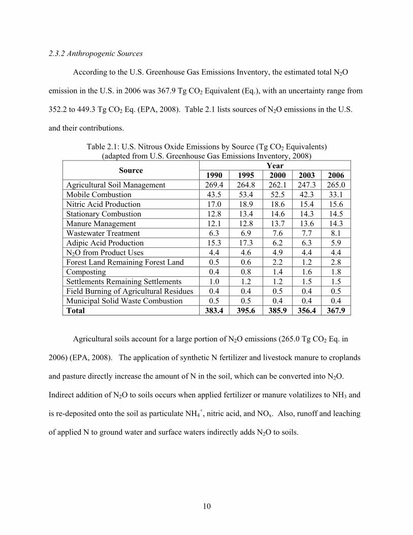
According to the U.S. Greenhouse Gas Emissions Inventory, the estimated total N2O
emission in the U.S. in 2006 was 367.9 Tg CO2 Equivalent (Eq.), with an uncertainty range from
352.2 to 449.3 Tg CO2 Eq. (EPA, 2008). Table 2.1 lists sources of N2O emissions in the U.S.
and their contributions.
Table 2.1: U.S. Nitrous Oxide Emissions by Source (Tg CO2 Equivalents) (adapted from U.S. Greenhouse Gas Emissions Inventory, 2008)
Year Source 1990 1995 2000 2003 2006 Agricultural Soil Management 269.4 264.8 262.1 247.3 265.0 Mobile Combustion 43.5 53.4 52.5 42.3 33.1 Nitric Acid Production 17.0 18.9 18.6 15.4 15.6 Stationary Combustion 12.8 13.4 14.6 14.3 14.5 Manure Management 12.1 12.8 13.7 13.6 14.3 Wastewater Treatment 6.3 6.9 7.6 7.7 8.1 Adipic Acid Production 15.3 17.3 6.2 6.3 5.9 N2O from Product Uses 4.4 4.6 4.9 4.4 4.4 Forest Land Remaining Forest Land 0.5 0.6 2.2 1.2 2.8 Composting 0.4 0.8 1.4 1.6 1.8 Settlements Remaining Settlements 1.0 1.2 1.2 1.5 1.5 Field Burning of Agricultural Residues 0.4 0.4 0.5 0.4 0.5 Municipal Solid Waste Combustion 0.5 0.5 0.4 0.4 0.4 Total 383.4 395.6 385.9 356.4 367.9
Agricultural soils account for a large portion of N2O emissions (265.0 Tg CO2 Eq. in
2006) (EPA, 2008). The application of synthetic N fertilizer and livestock manure to croplands
and pasture directly increase the amount of N in the soil, which can be converted into N2O.
Indirect addition of N2O to soils occurs when applied fertilizer or manure volatilizes to NH3 and
is re-deposited onto the soil as particulate NH4+, nitric acid, and NOx. Also, runoff and leaching
of applied N to ground water and surface waters indirectly adds N2O to soils.
10

Nitrous oxide emissions from livestock manure and urine also occurs through
nitrification and denitrification. The amount of N2O produced depends on the composition of the
manure and urine, the type of bacteria present, and the amount of oxygen and liquid present.
Emissions of N2O from manure management were estimated at 14.3 Tg CO2 Eq. for the year
2006.
Nitrous oxide emissions also result from the reaction that occurs between N and oxygen
during fossil fuel combustion. The type of fuel and pollution control device used as well as the
maintenance and operating practices affect the amount of N2O emitted. Catalytic converters on
vehicles can promote the formation of N2O, although the latest technical modifications to
converters are addressing this problem. From 1990 to 2006, N2O emissions from mobile
combustion decreased by 24 percent. The total N2O emission from mobile combustion was 33.1
Tg CO2 Eq. in 2006 (approximately 9 percent of total U.S. N2O emissions).
Nitric acid production accounts for 15.6 Tg Eq. CO2 for N2O emissions in 2006 while
adipic acid production accounts for 5.9 Tg CO2 Eq. Nitric acid is used for production of
synthetic fertilizers, adipic acid, and explosives.
Wastewater treatment plants are another anthropogenic source of N2O emissions, where
human sewage and other household wastewater end up. Nitrous oxide emissions result from
both nitrification and denitrification of the N present in the wastewater, usually in the form of
urea, ammonia, and proteins. Wastewater treatment plants account for 8.1 Tg Eq. CO2 of N2O
emissions.
11

2.4 Factors that Affect N2O Emissions
There are many factors regulating the loss of N2O from croplands to the atmosphere.
Section 2.4.1 will discuss the role of nitrification and denitrification in N2O emissions. In
section 2.4.2, the role of crop management will be discussed.
2.4.1 Nitrification and Denitrification Rates
The microbial process of denitrification and nitrification are the major sources of N2O
emission from the soil. Nitrification is the biological oxidation of ammonium (NH4+) to nitrite
(NO2-) or nitrate (NO3
-) under aerobic conditions and N2O is a byproduct of nitrification
(Seinfeld and Pandis, 1998). In denitrification, which is the bacterial process of converting
nitrate (NO3-) to dinitrogen (N2) and N2O under anaerobic conditions, N2O is an intermediate
(Seinfeld and Pandis, 1998). Nitrification rates are relatively uniform throughout a field while
denitrification rates vary temporally and spatially (IFA, 2001). Various factors control whether
nitrification or denitrification dominates in the production of N2O.
Haverkort and MacKerron (2000) and the International Fertilizer Industry Association
(IFA) (2001) have summarized the factors that affect nitrification and denitrification in crop
production. They concluded that in most soils, nitrification depends on the amount of NH4+ and
oxygen in the soil as well as the soil pH and temperature. The amount of NH4+ in the soil is
derived from either mineralization of organic matter or from applied N fertilizer. Nitrification
activity is generally suitable for pH levels between 4 to 8, and at high pH values (pH > 8) it may
be inhibited due to toxic effects to the bacteria. When the soil temperature is above 4 °C,
nitrification activity is favorable and is optimized when the soil temperature is between 20-40
°C. The factors that control nitrification are not the same for denitrification.
12

Denitrification depends on soil components such as the availability of organic carbon (C),
oxygen, and NO3-. Organic compounds, such as organic C, serve as electron donors and are
sources of bacterial cellular material for denitrification activity. As soil oxygen content
decreases, denitrification activity increases since anaerobic conditions are required for both
synthesis and activity of the enzymes involved in the denitrification process. Denitrification
rates generally increase linearly with NO3- concentrations up to 40 mg L-1, while at relatively
high NO3- concentrations denitrification is independent of NO3
- concentration.
Similar to nitrification, the soil pH controls bacterial denitrification activity. Under
acidic conditions (pH < 7), denitrification rates are slower than in alkaline conditions (IFA, 2001,
Haverkort and MacKerron, 2000). In contrast to nitrification, soil temperature does not control
denitrification activity because soil denitrifiers are adapted to and are capable of growing under a
wide range of temperatures (Haverkort and MacKerron, 2000).
Other controlling factors for denitrification include the presence of decomposing organic
matter and the magnitude of NH3 volatilization. The presence of decomposing soil organic
matter and plant litter produces anaerobic areas where high denitrification rates occur. NH3
volatilized from applied fertilizer can be re-deposited onto the soil, indirectly affecting the
availability of N for nitrification or denitrification (Haverkort and MacKerron, 2000).
2.4.2 Management Practices
Various agricultural management activities affect N2O emissions from soils. Such
activities include the application of nitrogen and excessive water and soil tillage. Nitrogen
inputs to the soil, such as N fertilizer, animal manure, and crop residues, increase the amount of
N available for nitrification and denitrification. Thus, N2O emissions may increase with the N
application rate. The production of N2O is also related to the timing of fertilizer application.
13

When NH4+-based fertilizers are applied to the soil under conditions suitable for nitrification
activity without any competition from plant uptake, N2O emissions are likely to increase (IFA,
2001). This is also true when NO3--based fertilizers are applied to soil under conditions suitable
for denitrification activity.
Soil moisture is another factor since the soil moisture content affects the diffusion of
oxygen through the soil. The rate of N2O emission increases as the water-filled pore space
(WFPS) in the soil increases. High N2O emissions have been observed when the WFPS is
between 60 and 90%, when the production of N2O is dominated by denitrification (Dobbie et al.,
1999, IFA, 2001, Flessa et al., 2002). High water content may result from heavy rain or
excessive rates of irrigation. Below 60% WFPS nitrification, an aerobic process, is the dominant
process for the production of N2O (IFA, 2001).
Also, localized spatial variations in micro-relief (such as ridges and furrows or raised
beds) or in water infiltration rates due to compaction, can result in localized wet spots. Usually,
greater N2O emission rates occur from tractor-compacted furrows than from ridges due to a
greater reduction of air-filled pore space (Flessa et al., 2002, Smith et al., 1997). Flessa et al.
(2002) measured mean WFPS values of 61% for tractor compacted inter-rows, 49% for
uncompacted inter-rows, and only 30% for ridges for the growing period of potato fields in
Germany.
Soil tillage may induce enhanced organic N mineralization (IFA, 2001). Soil tillage is
typically conducted during planting and harvesting of root/tuber crops, and is the process of
digging up the soil for the purpose of incorporating plant residues and/or fertilizer, seedbed
preparation, weed control, and soil and water conservation. Soil tillage affects the gas diffusivity
within the soil and the water and air holding capacity of the soil pores.
14

2.4.3 Other Factors
Soil properties, such as soil texture, affect N2O emissions. Fine-textured soils hold water
more tightly because they have more capillary pores within aggregates than sandy soils. Thus, in
fine-textured soils, anaerobic conditions are easily maintained for longer periods of time (IFA,
2001).
Gas diffusion also has an influence on emissions of N2O since before being emitted to the
atmosphere, the N2O gas must first diffuse through the soil pores. High soil water content,
impeded drainage, soil compaction, fine soil texture, and soil surface sealing can all limit gas
diffusion through the soil. Haverkort and MacKerron (2002) state that high denitrification
activity may be present in soils that are close to saturation, but the emission of N2O from the soil
can be low. Thus, anaerobic conditions promote denitrification but limits gas diffusion.
2.5 Emission Rates of N2O
The increase in atmospheric N2O concentration of two to three percent every year is well
documented but the sources of the increase are not (Vitousek et al., 2000). Nitrous oxide
emissions from agriculture are typically reported as an emission factor (EF), which is the amount
of N2O emitted as a percentage of the N fertilizer applied. A default mean EF of 1.25 ± 1% of
the N fertilizer applied was adopted by the Intergovernmental Panel on Climate Change (IPPC)
in 1997 (Bouwman, 1996). This default EF is based on experiments that were at least 1 year in
duration. The default EF is a general approximation and is independent of the specific crop type,
region, environment, and management practices. Documented EF values range from 0.1 to 7.8%
(Dobbie and Smith, 2003). The use of the default mean EF value is highly uncertain since there
are extremely high spatial, temporal, inter-annual, and crop type variability in N2O emissions.
15

Dobbie et al. (1999) measured N2O emissions from intensively managed fields of
ryegrass, winter wheat, potatoes, broccoli, and oilseed rape in Scotland. The fields of grassland,
winter wheat, potato, and oilseed rape were treated with ammonium nitrate fertilizer. An
ammonium nitrate/ammonium/phosphate/urea fertilizer mix was applied to the broccoli fields.
Nitrous oxide fluxes varied widely throughout the year at all sites and also between sites.
Emissions from the winter wheat, barley, and oilseed rape fields (0.2 to 0.7 kg N2O per 100 kg
applied N; EF: 0.2 to 0.7%) were consistently lower than emissions from the fields of grassland,
potato, and broccoli (0.3 to 5.8 kg N2O per 100 kg applied N; EF: 0.3 to 5.8%). Daily fluxes
were as high as 1.2 kg N2O hectare-1 day-1 and annual emissions ranged from 0.3 to 18.4 kg N2O
hectare-1 year-1. At all sites, fluxes generally increased sharply after N-fertilizer additions and
gradually decreased with time. All of the reported emission rates were obtained from flux
measurements using chambers.
Flessa et al. (2002) reported mean N2O emissions of 1.6 and 2.0 kg hectare-1 for the 1997
and 1998 growing periods (end of May to September) of two adjacent potato fields in Germany.
The fields were applied with 75 and 37 kg N hectare-1 for 1997 and 1998, respectively, resulting
in EF values of 2.1% and 5.4%. Flessa et al. obtained these emission rates from flux
measurements made by automated gas sampling chambers.
Haile-Mariam et al. (2008) reported N2O losses of 0.5% (0.55 kg N hectare-1) of applied
fertilizer (112 kg N hectare-1) in corn fields and 0.3% (0.59 kg N hectare-1) of 224 kg N hectare-1
applied fertilizer in potato fields in central Washington during the 2005 and 2006 growing
seasons. The fields were applied with urea-ammonium-nitrate (UAN) solution (32% N) through
a center pivot irrigation system. The fields were under sweet corn–potato rotation. Aerobic soil
16
17
conditions dominated, with soil WFPS ranging from 0.50–0.63 m3 m-3. Gas samples were
collected using static chambers.
2.6 Sources of Ammonia (NH3)
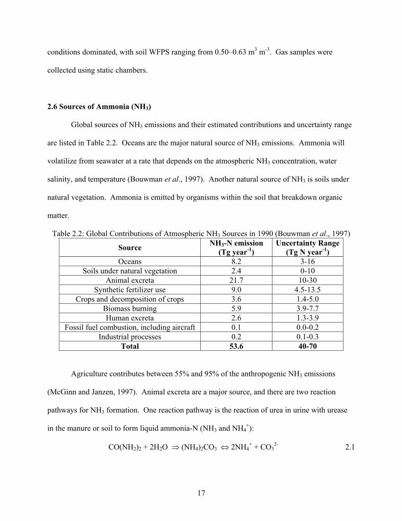
Global sources of NH3 emissions and their estimated contributions and uncertainty range
are listed in Table 2.2. Oceans are the major natural source of NH3 emissions. Ammonia will
volatilize from seawater at a rate that depends on the atmospheric NH3 concentration, water
salinity, and temperature (Bouwman et al., 1997). Another natural source of NH3 is soils under
natural vegetation. Ammonia is emitted by organisms within the soil that breakdown organic
matter.
Table 2.2: Global Contributions of Atmospheric NH3 Sources in 1990 (Bouwman et al., 1997)
Source NH3-N emission (Tg year-1)
Uncertainty Range(Tg N year-1)
Oceans 8.2 3-16 Soils under natural vegetation 2.4 0-10
Animal excreta 21.7 10-30 Synthetic fertilizer use 9.0 4.5-13.5
Crops and decomposition of crops 3.6 1.4-5.0 Biomass burning 5.9 3.9-7.7 Human excreta 2.6 1.3-3.9
Fossil fuel combustion, including aircraft 0.1 0.0-0.2 Industrial processes 0.2 0.1-0.3
Total 53.6 40-70
Agriculture contributes between 55% and 95% of the anthropogenic NH3 emissions
(McGinn and Janzen, 1997). Animal excreta are a major source, and there are two reaction
pathways for NH3 formation. One reaction pathway is the reaction of urea in urine with urease
in the manure or soil to form liquid ammonia-N (NH3 and NH4+):
CO(NH2)2 + 2H2O ⇒ (NH4)2CO3 ⇔ 2NH4+ + CO3
2- 2.1

18
Ammonia emissions from urine deposited in natural areas are lower than from high
density areas where animals are domesticated. The second reaction pathway is the
microbiological anaerobic breakdown of organic N. Increasing human population, and therefore
increasing food demand, has led to more domesticated animals and increased NH3 emissions
(Vitousek et al., 1997). Ammonia emissions also result from sprinkler application of dairy
lagoon slurry from milking cows (Rumburg et al., 2006).
Application of synthetic fertilizer to croplands is another anthropogenic source of NH3
emissions. Up to 50% of the applied N to croplands can be lost through gaseous emissions,
leaching, runoff, or erosion. Generally, the dominant N loss processes are through gaseous
emissions, mainly from volatilization of NH3 and denitrification (IFA, 2001). Ammonia
emissions can come from both soil and crop foliage. Ammonia emissions from soil depend on
factors such as soil properties (i.e. soil pH, water content, and porosity). From crop foliage, the
emissions depend on the plant developmental stage and a compensation point of atmospheric
NH3, below which vegetation acts as a source and above which vegetation acts as a sink (Lemon
and van Houtte, 1980 as cited in McGinn and Janzen, 1997). Other factors such as the type and
quantity of fertilizer applied and meteorological factors (i.e. wind speed, temperature, and
precipitation) affect NH3 emissions from soil and crop foliage.
Another source of NH3 is from human breath, sweat, and waste. Emissions of NH3 from
treatment systems of human waste result from anaerobic degradation and are not well studied
(Bouwman et al., 1997).
Incomplete combustion of fossil fuels also produces NH3 emissions. Information on NH3
emissions from fuel combustion is scarce and associated with large uncertainties (Bouwman et
al., 1997). The use of emission controls in car engines to reduce NO and NO2 emissions has led
18
to increased NH3 emissions. Vehicles with three-way catalytic converters emit more NH3 than
cars with no emission controls (Bouwman et al., 1997). The combustion of coal and natural gas
and industrial processes (i.e. production of explosives) also contribute to NH3 emissions.
2.7 Regulating Factors of NH3 Emission
There are many factors regulating the loss of NH3 from soil-plant systems to the
atmosphere. Section 2.7.1 will discuss factors that affect NH3 emissions from the soil. In
section 2.7.2, the factors that affect NH3 emissions from the crop foliage will be discussed.
2.7.1 NH3 Emissions from Soil
Emissions of NH3 from soils result from biological degradation of organic compounds
and are dependent on the following factors: the transformations of the total ammonicial N (TAN)
in the soil, which include NH3-N + NH4+-N, the soil properties, climatic factors, management
practices, and the partial pressure between the atmosphere and the soil.
The NH4+ in the fertilizer applied can be bacterially nitrified to nitrate (NO3
-), converted
to NH3, or remain as NH4+ (Bouwman and Bouman, 2002). Ammonium will be in equilibrium
with NH3 depending upon the pH of the solution, as shown in the following reaction:
NH3 + H2O ↔ NH4+ + OH- 2.2
Soil properties such as soil pH, moisture content, infiltration rate, and cation exchange
capacity (CEC) affect the rate of NH3 volatilization from the soil to the atmosphere. Ammonia
volatilization increases with increasing pH; the greatest NH3 volatilization occurs when the soil
pH is greater than 7.5 (Liu et al., 2007). From 0 to 30 % soil water content, the amount of NH3
emission increases with increasing moisture due to the inability of the NH3 molecules to displace
water molecules (IFA, 2001). When the soil water content increases from 30 % to 100 %, NH3
19

emissions decrease due to dissolution of NH3 in the soil (IFA, 2001). The CEC is the capacity of
a soil for ion exchange of positively charged ions between the soil and the soil solution. The
lower the CEC, the more likely it is for NH3 volatilization to occur (Bouwman and Bouman,
2002; Haverkort and MacKerron, 2000).
Climatic factors, such as wind speed and temperature, also affect NH3 volatilization from
the soil. Increasing wind speed promotes more rapid transport of NH3 away from the water or
soil to the atmosphere (Bouwman and Bouman, 2002; Haverkort and MacKerron, 2000). As soil
temperature increases, the relative proportion of NH3 to NH4+ increases while the solubility of
NH3 in water decreases (Bouwman and Bouman, 2002). Ammonia emissions may also increase
as conditions of stress caused by crop disease, pests, and/or adverse weather conditions, such as
drought, occur (Heckathorn and DeLucia, 1995 as cited in Bouwman et al., 1997).
The method and rate of fertilizer application can have a significant effect on the amount
of NH3 loss from fertilizer applications. Generally, applications that effectively bury the
fertilizer (i.e. banding) result in lower NH3 loss (IFA, 2001, Potter et al., 2001). While the effect
of fertilizer application type is fairly well understood, studies conducted on the effect of N
fertilizer application rate and the amount of NH3 volatilization show conflicting results (IFA,
2001). Some studies reveal higher NH3 volatilization rates at high N application rates while
other studies show the opposite result.
The type of fertilizer applied influences the emissions of NH3 since different types of
fertilizer contain various percentages of N. When urea fertilizer is applied to very moist soils,
the urea is hydrolyzed by the enzyme urease to produce a mixture of NH3, NH3+, and bicarbonate
(HCO3-) by the following reaction (Sommer et al., 2004):
CO(NH3)2 + 2H2O ↔ NH3 + NH4+ + HCO3
- 2.3
20

The rate at which urea is hydrolyzed is related to urease activity, the availability of water, the pH
of the solution, and temperature. The rate increases as water content and pH increases. Soil
urease activity is optimized when the soil pH is between 8 and 9. The rate of urea hydrolysis
also increases as temperature increases.
Ammonia volatilization is also driven by the atmospheric NH3 concentration, and occurs
when atmospheric NH3 concentration is lower than the NH3 concentration in the soil, liquid, or
intercellular air space of the plant leaves (Bouwman and Bouman, 2002).
2.7.2 NH3 Emissions from Crop Foliage
Plant leaves are another source of NH3 emissions. Dissolved NH3 and NH4+ can be found
in the water film, also known as the apoplastic solution, in the mesophyll cell walls of plant
leaves. The amount of NH3 and NH4+ dissolved depends on the plant developmental stage,
climate, fertilization, and the difference between the atmospheric NH3 concentration and the NH3
concentration in the leaves (Sommer et al., 2004). Ammonia will be emitted from a leaf if the
leaf NH3 concentration is greater than the atmospheric NH3 concentration and NH3 will be
absorbed by the leaf in the reverse situation. Another source of NH3 emission is decomposing
potato tops and other plant residues. Generally, NH3 volatilization increases with moisture,
temperature, and N content of plant residues.
2.8 Emission Rates of NH3
Agriculture is the largest source of global NH3 emissions. Up to 50% of the applied N to
croplands can be lost with gaseous emissions being the dominant N loss mechanism (IFA, 2001).
There is a great deal of uncertainty in the magnitude of NH3 emissions from various croplands.
There are many factors that affect the emission rates and only a limited number of studies on the
21
emissions are available. A standard emission rate of 2.5 kg N hectare-1 year-1 has been used for
all agricultural crops when compiling global emissions inventories, which contains a high degree
of inaccuracy (Bouwman et al., 1997). Current U.S. emission estimates are based upon
European measurements, which are not representative of actual farming practices in the U.S.
The IFA (2001) reports that there is a clear difference between measurements carried out
in the fields and those performed inside laboratories. In addition, the measurement method used
and the location where the measurements are made significantly affects the emission rates while
the crop type is less significant (IFA, 2001). The average NH3 emission rates from grass are
generally 20 and 10% lower than from upland crops (croplands with no standing water
throughout the growing season; i.e. corn and potato fields) and flooded systems, respectively
(IFA, 2001).
The IFA (2001) report has grouped NH3 volatilization rates from upland crops by
fertilizer type applied. Using micrometeorological techniques, the reported NH3 loss from
broadcast applied UAN fertilizer ranges from 8% to 18%, with an average of 15%. Broadcast
application typically involves spreading dry fertilizer over the soil surface. Using dynamic flow
chambers, the reported NH3 loss varies from negligible to 45%. For the potato fields used for
this study, UAN fertilizer was applied using a center-pivot irrigation system. From upland crops
applied with ammonium bicarbonate, an NH3 loss rate of 21% was measured in a field study
using static chambers. Higher NH3 loss rates (as high as 30 to 70%) were measured in a
laboratory study using dynamic flow chambers. From calcium ammonium nitrate applications,
NH3 loss rates of up to 6% were reported from laboratory studies and much lower rates from
field studies. Both the laboratory and field studies used dynamic flow chambers. Ammonia
losses from upland crops applied with urea range from 15 to 20%. This range comes from
22

23
various measurement techniques including chambers with and without forced flow,
micrometeorological techniques, and wind tunnel measurements.
Studies have shown that the magnitude of NH3 emissions resulting from decomposition
of crop residue depends on the N content in the residue (McGinn and Janzen, 1997). In a study
on perennial ryegrass herbage, 10% of the NH3 applied was emitted to the atmosphere from
herbage with 29.8 mg N g-1 of leaf biomass, and no losses from herbage with 9.2 mg N g-1 leaf
biomass. In another study, 14% of the N applied was emitted into the atmosphere for a legume
green manure (McGinn and Janzen, 1991). In the U.K., it is estimated that volatilized N losses
by grassland decomposition accounts for 2.7% of the total N emissions in agriculture (Whitehead
and Lockyer, 1989 as cited in McGinn and Janzen, 1997). Measured NH3 emissions from
decomposing sugar beet leave, potato tops, and field beam straw range from 0.9 to 3.7% of the N
content (Sommer et al., 2004).
Little information is known on NH3 volatilization losses in potato fields. The potato
plant’s N uptake efficiency under current best management practices is approximately 65%
(Lang et al., 1999) with a mean of 40% (Balasubramanian et al., 2004). Measured NH3
emission rates from barley, wheat, and oilseed rape canopies range from 1 to 15 kg hectare-1
year-1 while measured NH3 emissions from sugar beet leaves and potato shoots ranged from 8.6
to 12.6 kg N hectare-1 year-1 (Sommer et al., 2004).

24
CHAPTER 3
METHODOLOGY
This chapter describes the methods used for measuring N2O and NH3 concentrations and
for determining flux rates from the potato fields. Mixing ratios of N2O were measured using gas
chromatography (GC) and flux rates of N2O were estimated using a static chamber method. A
short-path differential optical absorption spectroscopy (DOAS) instrument was used to measure
concentrations of NH3 along a path downwind of the fields. Sulfur hexafluoride (SF6) was
released from a point source from the center pivot of the fields to simulate NH3 plume dispersion
and to calibrate a Gaussian plume model (SIMFLUX). SIMFLUX was then used in an inverse
modeling approach to estimate flux rates of NH3 from the fields. Data were collected at potato
fields in central WA, near Othello.
3.1 Measurement of N2O
A disjunct eddy accumulation (DEA) system was used in summer 2006 for measurement
of N2O fluxes. In operation, air samples are partitioned into updraft and downdraft reservoirs
over some averaging period based on the sign of the vertical velocity (Turnipseed et al., 2008).
The total flux is related to the concentrations in the updraft and downdraft reservoirs. It was
found that N2O flux measurements with the DEA were below detection limits and so a static
chamber method was then used for the summers of 2007 and 2008. For more information on the
DEA system, refer to Turnipseed et al. (2008).
24
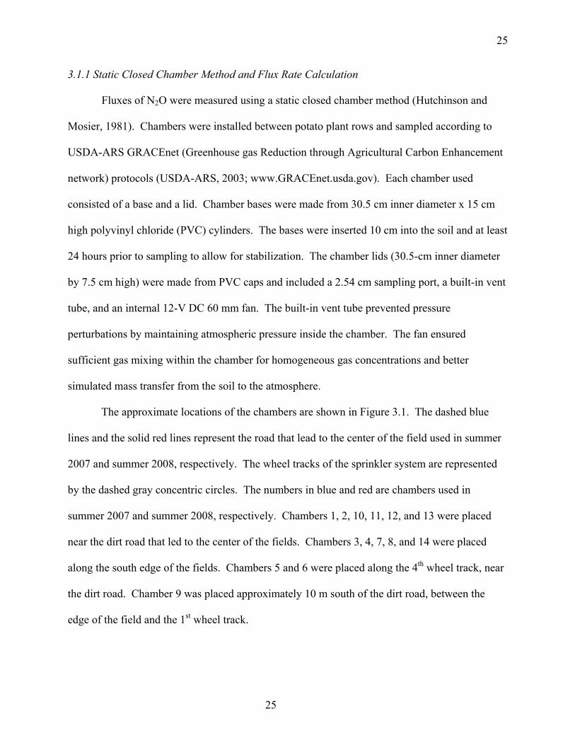
25
3.1.1 Static Closed Chamber Method and Flux Rate Calculation
Fluxes of N2O were measured using a static closed chamber method (Hutchinson and
Mosier, 1981). Chambers were installed between potato plant rows and sampled according to
USDA-ARS GRACEnet (Greenhouse gas Reduction through Agricultural Carbon Enhancement
network) protocols (USDA-ARS, 2003; www.GRACEnet.usda.gov). Each chamber used
consisted of a base and a lid. Chamber bases were made from 30.5 cm inner diameter x 15 cm
high polyvinyl chloride (PVC) cylinders. The bases were inserted 10 cm into the soil and at least
24 hours prior to sampling to allow for stabilization. The chamber lids (30.5-cm inner diameter
by 7.5 cm high) were made from PVC caps and included a 2.54 cm sampling port, a built-in vent
tube, and an internal 12-V DC 60 mm fan. The built-in vent tube prevented pressure
perturbations by maintaining atmospheric pressure inside the chamber. The fan ensured
sufficient gas mixing within the chamber for homogeneous gas concentrations and better
simulated mass transfer from the soil to the atmosphere.
The approximate locations of the chambers are shown in Figure 3.1. The dashed blue
lines and the solid red lines represent the road that lead to the center of the field used in summer
2007 and summer 2008, respectively. The wheel tracks of the sprinkler system are represented
by the dashed gray concentric circles. The numbers in blue and red are chambers used in
summer 2007 and summer 2008, respectively. Chambers 1, 2, 10, 11, 12, and 13 were placed
near the dirt road that led to the center of the fields. Chambers 3, 4, 7, 8, and 14 were placed
along the south edge of the fields. Chambers 5 and 6 were placed along the 4th wheel track, near
the dirt road. Chamber 9 was placed approximately 10 m south of the dirt road, between the
edge of the field and the 1st wheel track.
25

Figure 3.1: Locations of the chambers used for N2O flux measurements. Blue marks represent the field in 2007, and red marks represent the field in 2008.
N
13
12
11
10
3 4
6 5
14
9 2
1
dirt road
W
dirt road
E
S
8 7
Air samples (about 30 ml) from within the chambers were collected every 15 minutes
over a period of 1 hour after covering the chambers. After the first 1 hour of sampling, the
chamber was uncovered for 30 minutes before the second hour of sampling began. Typically, a
total of 4 hours of sampling was conducted for each chamber. To calculate the flux of N2O,
linear regression and the following calculation was used:
3.1
The gas flux values were converted from a volumetric basis to a mass basis.
26

3.1.2 Advantages and Disadvantages of using the Chamber Method
The advantages of using the chamber method is that chambers are relatively inexpensive,
easy to build, install, and remove, and have low detection limits. The disadvantages of using
chambers include the inability to account for environmental conditions (i.e. winds) and
disturbance to the soil which can easily occur when installing chamber bases. In addition, the
method is labor intensive. Five air samples are needed to calculate one flux rate value. Chamber
bases need to be installed at least 24-hours prior to sampling to minimize soil disturbance and
root damage. Careful planning of sampling time is necessary to ensure that the measurements
are made immediately after spraying of water or water with N fertilizer by the sprinkler system.
Finally, numerous chambers are needed to capture the variability of N2O flux rates through the
field due to heterogeneity of the soil.
3.1.3 Sample Analysis
Gas sampling was performed 0 to 6.5 hours after fertigation and irrigation events.
Analysis of air samples for N2O concentration was conducted using a Hewlett-Packard 5890 Gas
Chromatograph (GC) with an Electron Capture Detector (ECD). An ECD is best for analysis of
compounds containing halogens and nitro groups (Poole and Poole, 1991). An Alltech Porapak
Q (80/100) column was used and kept isothermal at 40 °C. The carrier gas was 95% Argon (Ar)
and 5% methane (CH4). The GC flow rate ranged from 24.5 to 25.5 standard cubic centimeters
per minute (sccm) and was maintained using an Alltech Digital Flow Check Flow Meter. A 777
ppbv N2O ± 10% (Scott-Marrin) standard was analyzed multiple times during each sampling
day. All samples were analyzed within one day of collection since tests showed decreased
concentrations (~25% reduced) from syringes analyzed after 24 hours.
27

3.2 Measurement of NH3
3.2.1 Differential Optical Absorption Spectroscopy (DOAS)
Spectroscopy is the study of the interaction between radiation and matter as a function of
wavelength (λ). Gas molecules absorb radiation if the radiation can electronically excite or
change the vibrational or rotational energy of the molecule. A short-path differential optical
absorption spectroscopy (DOAS) technique was used to measure NH3 emissions from the potato
fields. The DOAS technique avoids the NH3 adhesion problem (Mount et al., 2002) that is
common with in-situ methods using inlets and sampling tubes.
The DOAS technique measures the spectroscopic molecular absorption of trace gases
over an open atmospheric path. Using Beer’s Law, which relates the amount of light absorbed to
the number of molecules in the measurement path length, the concentration of NH3 can be
calculated. Beer’s Law states that there is a logarithmic dependence between the transmissivity
of light through a substance and the product of the absorption coefficient of the molecule and the
distance the light travels through the material. Beer’s Law can be expressed as:
T = I(λ)/Io(λ) = exp-∑σi(λ)LNi 3.2
T - transmissivity;
λ - wavelength [nanometers];
I(λ) - light intensity in the presence of absorbers [counts];
Io(λ) - light intensity without absorbers [counts];
σi(λ) - absorption cross-section of the ith absorber expressed in [cm2];
Ni - concentration of the ith absorber [molecules cm-3];
L - distance that the light travels through the material or the path length [cm].
28
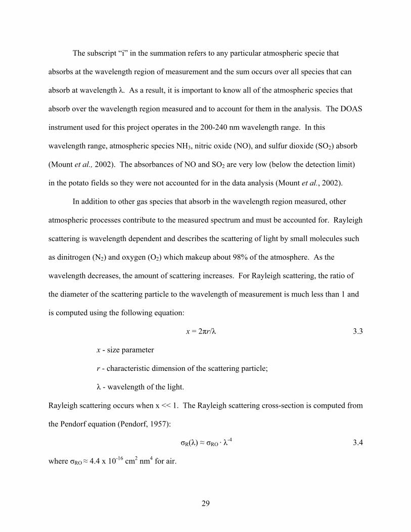
The subscript “i” in the summation refers to any particular atmospheric specie that
absorbs at the wavelength region of measurement and the sum occurs over all species that can
absorb at wavelength λ. As a result, it is important to know all of the atmospheric species that
absorb over the wavelength region measured and to account for them in the analysis. The DOAS
instrument used for this project operates in the 200-240 nm wavelength range. In this
wavelength range, atmospheric species NH3, nitric oxide (NO), and sulfur dioxide (SO2) absorb
(Mount et al., 2002). The absorbances of NO and SO2 are very low (below the detection limit)
in the potato fields so they were not accounted for in the data analysis (Mount et al., 2002).
In addition to other gas species that absorb in the wavelength region measured, other
atmospheric processes contribute to the measured spectrum and must be accounted for. Rayleigh
scattering is wavelength dependent and describes the scattering of light by small molecules such
as dinitrogen (N2) and oxygen (O2) which makeup about 98% of the atmosphere. As the
wavelength decreases, the amount of scattering increases. For Rayleigh scattering, the ratio of
the diameter of the scattering particle to the wavelength of measurement is much less than 1 and
is computed using the following equation:
x = 2πr/λ 3.3
x - size parameter
r - characteristic dimension of the scattering particle;
λ - wavelength of the light.
Rayleigh scattering occurs when x << 1. The Rayleigh scattering cross-section is computed from
the Pendorf equation (Pendorf, 1957):
σR(λ) ≈ σRO · λ-4 3.4
where σRO ≈ 4.4 x 10⁻¹⁶ cm2 nm4 for air.
29

Mie scattering (clouds and aerosols) occurs when the particles causing the scattering are
larger than the wavelengths of radiation in contact with them. Similarly, Mie scattering can be
modeled as an absorption cross-section. The cross-section for Mie scattering depends on the
particles causing the scatter, but is typically given by λ-1.6. Since NH3 absorption is being
measured in the mid-ultraviolet range (below the atmospheric cutoff of 290 nm) the solar
spectrum does not need to be accounted for, a major benefit of measuring in this spectral region.
Accounting for Rayleigh and Mie scattering, Beer’s law becomes the following:
I(λ)/Io(λ) = exp[(-∑σi(λ)LNi) + ε R(λ) + ε M(λ)] 3.5
3.2.2 Instrument Description
Two versions of the instrument were used for NH3 measurements. Details of the
instrument used in summer 2007 are described in Mount et al. (2002). In this section, a brief
description of the original instrument will be presented, followed by a description of the revised
instrument.
A schematic diagram of the original DOAS instrument used for summer 2007
measurements is shown in Figure 3.2 and a picture of the instrument housing, which was a small
trailer, is shown in Figure 3.3. A 150 W xenon (Xe) high-pressure emission lamp (source region
of 0.5 mm, Hamamatsu Corp. model L2273) is used as a light source and is located at the side of
the optical path of the primary mirror. The light from the Xe lamp is directed onto the 1st folding
mirror, which then directs the light onto a f/5 parabolic primary mirror. The primary mirror is 40
cm in diameter, coated with aluminum (Al) and magnesium fluoride, and was made by Colorado
Precision Optics. Only an annulus of 6 cm of light is illuminated onto the primary mirror since
there is a second folding mirror that is located between the primary mirror and the 1st folding
mirror which blocks part of the beam.
30

Figure 3.2: Schematic drawing of the original DOAS instrument showing the optical light path from the Xe lamp to the Reticon detector (Figure adapted from Mount et al., 2002).
primary mirror
spectrograph
Xe lamp
2nd folding mirror 1st folding
mirror
Figure 3.3: The original DOAS instrument housing (cover removed), which was a trailer (Figure adapted from Mount et al., 2002).
31

32
From the primary mirror, the annulus of light is directed towards a set of four large retro-
reflectors or a set of thirty-seven small retro-reflectors mounted on a tripod. Each of the four big
retro-reflectors is 12.7 cm in diameter, and each of the small retro-reflectors is 9 cm in diameter.
All are coated with Al and magnesium fluoride for protection. The retro-reflectors were
obtained from Melles Griot Inc. The light from the retro-reflectors is displaced and returned to
the primary mirror. The light is then intercepted by the second folding mirror, which directs the
light towards the slit of a double crossed Czerny–Turner spectrograph. The focal length of the
telescope optical system is 200 cm.
Inside the spectrograph, the light hits the 1st collimating mirror to make the rays parallel
before it is reflected to a diffraction grating. The grating breaks the light up into its constituent
colors. From the grating, the light travels to the 1st focusing mirror and then enters another
entrance aperture. Once again, the light passes through a 2nd set of collimating mirror, grating,
and focusing mirror. The spectrographs were double-crossed to reduce scattered light. The
detector used for the original DOAS instrument was a homebuilt Reticon silicon photodiode
array with 1024 pixels with each pixel 25 μm wide and 2.5 mm high. Spectral coverage was
about 60 nm and spectral resolution was about 0.6 nm.
The original DOAS instrument had several limitations. The computer used to control the
system was a Macintosh IIfx, which has been long discontinued. In addition, transporting the
trailer to and into an agricultural field was laborious. Pulling the trailer had to be done carefully
because the optics, detector, and other parts of the instrument are delicate and there were
insufficient mountings to absorb the shock. In the field, the slightest movements of the trailer
(e.g. heating and expansion of the tires) would result in loss of signal due to misalignment.
32

33
During the undertaking of this project, several parts of the DOAS instrument were
revised from the prototype version used at the WSU dairy including the instrument housing,
telescope and its light feed, and the detector. The revised DOAS instrument is more compact
than the original instrument. The optics setup of the revised instrument is similar to the setup of
the original instrument but the spectrograph is placed below instead of to the side of the 2nd
folding mirror and the primary mirror. The primary mirror (made by Stevens Optical) is only 32
cm in diameter instead of 40 cm, which allows for a more compact design. The light reflected
from the retro-reflectors is returned to the primary mirror and then is intercepted by the 2nd
folding mirror, which directs the light downward to a 3rd folding mirror. The 3rd folding mirror
directs the light into the entrance slit of the spectrograph. The angle of this third folding mirror
is manually tilted in two axes by small motors so that peak light intensity can be directed into the
spectrograph entrance slit. The f/number of the optical system is the same as the one used in the
original instrument. A schematic diagram and a picture of the revised DOAS instrument are
shown in Figure 3.4 and 3.5, respectively.

34
Figure 3.4: Schematic drawing of the revised DOAS instrument showing the optical light path from the Xe lamp to the CCD detector. The top figures illustrate a view from the top of the instrument, the bottom figure shows the view from the side.
Xe lamp
spectrograph
primary mirror 2nd folding mirror
1st folding mirror
3rd folding mirror entrance
slit
Zinc lamp
View from the Side
3rd folding mirror
View from the Top (bottom level)
View from the Top (top level)
CCD detector
3rd folding mirror
double-crossed Czerny-Turner spectrograph 150 W Xe lamp
retro-reflector array
2nd folding mirror
1st folding mirror 32 cm primary f/5 mirror
Figure 3.5: The revised DOAS instrument with the cover removed.
34

35
The detector used in the revised instrument is a Princeton Instruments charge coupled
device (CCD) detector system (spec-10:400B) with 400 pixels x 1340 pixels, with each pixel
19.4 µm wide and 19.4 µm high, and the spectral direction in the long direction. More details
regarding the CCD detector can be found on the Princeton Instruments website under products-
spectroscopy cameras-Spec-10-CCD. The WinSpec Spectroscopy Software version 2.5.16.5 was
used for data collection. This software is compatible with Windows. A PC laptop was used for
control of the system.
The main optics of the revised version are assembled on a 1.82 m by 0.85 m bench which
is loaded in the back of a pickup truck. A special canopy was designed to house all of the
necessary equipment (instrument, retro-reflectors, generator, etc.) for transport purposes. Two
bicycle tires are attached to the sides of the instrument in order to maneuver the system in the
field. A winch and two removable ramps are used to load the instrument into the back of the
pickup truck. The instrument canopy rides on a set of six inflatable tires to increase stability
during transportation and help absorb shock. Figure 3.6 shows a picture of the revised
instrument housing.
35

Figure 3.6: The new housing (a pickup truck canopy) for the DOAS instrument, which is used for transporting the instrument.
To set up, the instrument is winched down the ramps. Four air jacks are attached to the
corners of the instrument bench. The air jacks lift the instrument off the ground and the
instrument is placed on three tripods. Unloading and set up of the instrument can be
accomplished by three or more people and typically takes several hours. Aligning and fine
tuning of the instrument to the retro-reflectors takes an additional several hours. Figure 3.7 is a
picture of the revised DOAS instrument when it is setup for taking measurements.
36

Figure 3.7: The revised DOAS instrument when it is setup for taking measurements.
3.2.3 Advantages and Disadvantages of the DOAS Technique
Use of the DOAS technique for measuring NH3 concentrations has many advantages over
traditional in-situ measurements (Mount et al., 2002). Ammonia adheres to surfaces, such as
inlet tubes and sampling cells, and the use of the DOAS technique eliminates this problem.
Results depend only on the quality of the independently measured cross-sections of the species
and the algorithm used for data analysis (Mount et al., 2002). Finally, the DOAS technique can
measure several gas species simultaneously (i.e. NO, SO2, NH3 for the wavelength region used).
The DOAS technique also has disadvantages. First, it is limited to molecular species that
have spectrally structured absorption cross-sections in the wavelength region of the
measurement. In addition, the DOAS technique is limited to times of good visibility. Rain and
snow make measurements impossible due to the strong attenuation in the UV-Visible region.
Lastly, the DOAS technique is labor intensive because the instrument must be monitored on an
hourly basis to keep the instrument properly aligned.
37

38
There are many uncertainties associated with solving the Beer’s Law equation (eq. 3.3).
I(λ) and Io(λ) are generally not measured over the same path since the Io measurement should not
have any of the measured species in it. This negatively affects the spectral residual analysis.
Changes in the instrument, such as lamp output, may occur due to changes in temperature and
pressure that occur between measurement of I(λ) and Io(λ). Generally these changes are very
low frequency in spectral occurrence and so do not affect the analysis.
Table 3.1: DOAS instrument characteristics
Reticon Detector pixel size
25 μm wide x 2.5 mm high
CCD Detector pixel size
20 μm x 20 μm
Spectrograph focal length
375 cm
Telescope focal length (original system) focal length (revised system)
200 cm 160 cm
Xe Lamp output power arc length spot size wavelength range average life output fluctuation
150 W 0.5 mm 185-2000 nm 3000 hrs 1%
Other path length detection limit: 2007 data (original system) 2008 data (revised system) spectral coverage
~250 m 5 ppbv 10 ppbv 200-240 nm

39
3.2.4 Data Collection
Data was collected using the Reticon detector in the summer of 2007 and using the new
CCD detector in the summer of 2008. The instrument was aligned towards the retro-reflectors so
that the return signal counts were maximized. The integration time, which depends on the path
length, was varied so that the maximum count rate was about 30,000 to 40,000 counts per
integration time. Spectra were co-added so that data was averaged over five minute intervals.
Before taking actual measurements the electronic noise (dark spectra) of the instrument
system was measured by placing a black slide in front of the entrance slit of the spectrograph and
using the same settings as for the actual spectra. Changes in detector temperature caused
changes in dark spectra. As a result, dark spectra measurements were also taken about every
hour and were co-added and averaged. The average dark spectra were subtracted from the actual
spectra measured (when the slide was removed). A zinc (Zn) emission lamp was placed in front
of the entrance slit every hour to provide a strong spectral line fiducial at 213.9 nm. The Zn
fiducial line was centered at a chosen pixel.
3.2.5 Limitations on Data Collection
Time was a major limitation for collection of data. Measurements had to be taken during
the short potato growing season. The farmers who owned the fields would often make sudden
changes to the fertigation and irrigation schedules. This would be due to uncontrollable changes
in the weather, the crop's reaction to the fertigation and/or irrigation, and the amount of fertilizer
and/or water available. Data collection was prohibited during times of chemigation (i.e.
herbicides and/or pesticides) application because of health concerns.
39

40
Problems with the instrument were encountered in the field. Changes to the DOAS
instrument were implemented without being fully tested (e.g. the replacement of the detector)
before being used for data collection. High outside air temperature caused a significant problem
with the CCD detector. The internal cooler of the CCD detector could not keep the detector cold
enough when the outside air temperature was above ~24 °C. This problem was anticipated but
not enough testing was performed prior to going to the fields and so a solution was initiated in
the field. At the potato field near Othello, WA, the average outside air temperature during the
afternoon was always above ~24 °C and even occasionally reached above 37 °C. An external
radiator was used with cooling lines running through an ice bath in order to keep the detector
running. However, variations in the dark current were sufficiently uncontrollable that the dark
subtractions could not always be performed correctly.
3.2.6 Limitations on Data Quality
Analysis of the optical arrangement in January 2009 showed the focal position of the
spectrograph was incorrect, which resulted in loss of light (signal). Lower signal to noise ratio
(s/n) resulted in lower precision. However, this should not have affected the actual
determinations of molecular concentration when sufficient NH3 was present. It was also
discovered that the mirrors within the spectrograph were not properly aligned and this resulted in
a degraded spectral resolution. The crude temperature regulation of the CCD detector caused
major problems with dark subtraction and overall had a significant negative effect on the
measurement.
Figure 3.8 is a plot of the CCD Detector quantum efficiency (QE) with respect to
wavelength. The QE, which is a measure of the detector’s electrical sensitivity to light, in the
wavelength region used (200 to 240 nm) was below 10%, which resulted in lower s/n ratio.
40

Figure 3.8: Quantum Efficiency (QE) of the CCD Detector (Model Spec-10:400B (blue line)) with respect to wavelength (figure adapted from Princeton Instruments Spec-10 Datasheet, www.princetoninstruments.com/products/speccam/spec10/dsheet.aspx).
The detection limit of the instrument depends on the magnitude of the spectral residuals
of the data, which is the remainder of the spectral ratio of I and Io after removal of the known
absorbers (NH3) as well as the spectrum of Mie and Rayleigh scattering. The residual spectrum
should be random noise, but this level of precision is never reached due to systematic errors in
the removal of the spectral signatures, detector temperature problems, and changes in the spectral
structure of the Xe lamp. The original DOAS instrument was sensitive to a few ppbv of NH3
while the revised version is only sensitive to at best 10 ppbv of NH3.
The revised instrument can clearly be improved with more testing and modifications.
Problems for our field work were accentuated by time constraints due to the late completion of
the modified instrument, resulting in insufficient testing before using at the fields. The optical
problems with the spectrograph resulted in degraded performance, but it was decided not to
change this once the data collection was started. The main effects caused a degradation of s/n
41

and precision. Problems in the design of the telescope and feed optics were corrected part way
through the experiment to increase the collection of light and significantly reduced the
integration time.
3.2.7 Data Analysis
To convert the absorbance of NH3 given by Beer’s law to concentration, a nonlinear least
squares fitting method was used. The method fits the pattern of the cross-section of each gas
molecule that absorbs in the wavelength range used to the natural logarithm of the ratio of I/ Io.
In this case, only the cross-section of NH3 was used since the absorbances of NO and SO2 were
found to be very low.
Figure 3.9 shows the cross-section spectra of NH3 in the mid UV spectral region. This
shows the ability of NH3 to absorb light as a function of wavelength. For summer 2007
measurements, three absorption lines were used to reduce the data. For the summer 2008 data,
only two absorption lines were used (wavelength range: 199nm to 207nm).
42

Figure 3.9: Ammonia absorption cross-section.
In addition to the cross-section spectra of NH3, the nonlinear least squares algorithm
accounts for the spectral pattern of Rayleigh and Mie scattering as well as the shift and stretch of
the two spectra being ratioed. Shift and stretch in the spectra can result from displacement of the
grating and detector as well as temperature changes experienced by the spectrograph. The
method minimizes the spectral residual of patterns in the data after removal of the molecular
spectra signatures.
Data analysis is conducted in two steps. First, a relative Io, containing NH3 features, was
chosen from the measurement data (same-day) and used for initial data reduction. The NH3
concentration for each measurement period was then calculated relative to the Io chosen. The
actual NH3 concentration was then determined by reducing the relative Io with an absolute Io, a
spectra with no NH3 features taken in the laboratory.
43

3.2.8 Characterization of Dispersion Conditions using Tracer Studies
During some measurement periods, SF6 tracer gas was released from the center of the
fields and concentrations measured along a crosswind sample line downwind of the fields to help
characterize local dispersion conditions. To conduct tracer studies, SF6 was released as a
continuous point source from ground-level at the center pivot of the field. The SF6 release rates
ranged from ~0.6 to ~0.7 L min-1. Air flow was maintained using a 1.00 SLPM Tylan mass flow
controller (S/N AA9605027) and a Tylan RO-32 control box. A BIOS International DryCal DC-
Lite Flow Meter was used check flow rates. Sulfur hexafluoride is ideal for tracer studies
because it is inert, concentrations can be measured with satisfactory accuracy at very low
concentrations, and ambient concentrations of SF6 are negligible. Even though SF6 has a higher
molecular weight (146.06 g mol-1) than NH3 (17.03 g mol-1), the effect of this is negligible since
turbulent diffusion is the dominant transport mechanism (Kaharabata et al., 2000).
Positioned downwind of the source were Trace Gas Automated Profile System (TGAPS)
sample lines and syringe samplers. TGAPS is an automated sampling and analysis system,
which continuously measures 5-minute averaged concentrations of SF6 at seven different
locations. The system draws air through 7 long inlet lines positioned along the length of the
DOAS measurement path and air from these inlets is pumped into a set of seven 10-L Tedlar
bags. While one set of 7 bags collects air samples, a second set of 7 bags is analyzed. During
analysis, air from each bag is drawn to a continuous SF6 analyzer (Flaherty et al., 2007).
Between the sample analysis and collection, the Tedlar bags are evacuated completely to ensure
that the bags are “clean” for the next sampling period.
Air samples were also collected using programmable, battery-operated syringe samplers.
Each syringe sampler contains 12 syringes, which sequentially collect 30-minute averaged air
44

samples. Each syringe sampler is enclosed in an aluminum case, which serves to protect the 12-
syringe unit inside. A sealed compartment inside the syringe sampler houses the electronics,
stepper motors, and clock. Krasnec et al. (1984) provides a complete description of the syringe
samplers used. The syringe samplers were also deployed along and beyond the DOAS
measurement path downwind of the field and tracer release to provide a measure of plume width.
A GC equipped with an ECD and coupled with an electronic integrator was used to
measure SF6 concentrations. The air samples were combined with hydrogen (H2) and then
passed through a packed bed of palladium catalyst, which converted the oxygen (O2) in the air to
water (H2O). Then, the air passed through a nafion tube with a countercurrent flow of N2 to
remove the H2O from the sample stream. The sample stream was then passed to the ECD, where
voltage changes due to the SF6 in the stream provided the signal for concentration. See Benner
and Lamb (1985) and Flaherty et al. (2007) for additional information about this type of detector
system. Calibration was performed using 1005 pptv, 1625 pptv, and 1462 pptv Scott-Marrin Inc.
calibration gases (certified accuracy ±5%). All samples were analyzed within a day of
collection.
3.2.9 Field Setup
Figure 3.10 is a diagram of the field setup. Southwest winds are predominant in the
central WA region. Thus, the DOAS instrument measurement path (path from the spectrograph
to the retro-reflectors) was setup outside the edge on the northeast quadrants of the potato fields
to capture the NH3 plume as it traveled along the wind trajectory. Path lengths varied from ~150
to ~250 m.
45

Tracer sample lines and syringe samplers were set up along the DOAS measurement path
and extended over a distance of 800 m so that ideally the entire plume of SF6 would be captured.
More details on how the dispersion studies were conducted will be provided in section 3.3.2.
Figure 3.10: Diagram of the field setup.
The only source of electrical power was at the center of the fields. As a result,
instruments used in the fields (i.e. DOAS instrument) were powered using portable generators.
A storage building with power located nearby was used to power other instruments such as the
N2O GC.
3.3 Measurement of Meteorological Variables
Meteorological information such as wind velocity, wind direction, and air temperature
were measured using a sonic anemometer at 10 Hertz frequency. Soil moisture and temperature
were measured using CS515s Water Content Reflectometers and copper/constantan
* * * * * 800 m
DOAS
Road to center Syringe Samplers & TGAPS Sample Lines
X X
X X
X SF6 Point Source Release
o Retro-reflectors
X
Sprinkler Predominant
46

thermocouples (Campbell Scientific Inc.), respectively. Campbell Scientific CR10 data loggers
were used to record data. Leaf stomatal conductance was measured using Decagon Devices
Hand Held Leaf Porometer.
3.4 Determining Emission Rates of NH3
A Gaussian plume dispersion model (SIMFLUX) was used with an inverse approach to
estimate NH3 emission rates. The first part of this section will present the basis of the Gaussian
plume dispersion equation (section 3.4.1) and in section 3.4.2, the details of SIMFLUX will be
presented.
3.4.1 The Gaussian Plume Dispersion Equation
The Gaussian plume dispersion model is useful for measuring the impacts of air pollutant
sources on air quality. After a release, individual particles move according to velocity
fluctuations which are random, resulting in a random distribution in each coordinate system. The
result of this random distribution is that the plume contains more particles near the center of
mass while fewer particles are present at increasing distances from the center of mass. It is
reasonable to assume a Gaussian concentration distribution based on measurements of typical
plumes and for ease of mathematical computation.
For a continuously emitting point source strength (Q) in grams per second (g s-1) at an
effective height (h) in meters above the ground, the concentration C at a receptor location x, y,
and z in grams per cubic meter is given by the equation:
⎥⎥
⎦
⎤
⎢⎢
⎣
⎡+=
+−−−−2
2
2
2
2
2
2)(
2)(
2
2),,( zzy
hzhzy
zy
eeeu
QzyxC σσσ
σπσ 3.6
47

where x is the downwind distance of the receptor from the source in meters (m), y is the
crosswind distance in meters, z is the height of the receptor above the ground in meters, u is the
wind speed in meters per second, and σy and σz are the horizontal and vertical diffusion
coefficients, respectively, in meters. A complete general overview of the Gaussian plume
equation is discussed by Hanna et al. (1982).
Requirements for the Gaussian dispersion models are homogeneous turbulence, uniform
flow, no loss of pollutants, and steady state conditions (Arya, 1999). In addition, mean wind
speed is required to be larger than the standard deviations of turbulent velocity fluctuations, so
that the upstream or longitudinal diffusion can be neglected. Thus, significant wind shears,
inhomogeneous turbulence, and weak winds make the theoretical basis of Gaussian dispersion
modeling invalid. Finally, the methods for obtaining certain input parameters used in the
Gaussian plume dispersion equation are also subject to many assumptions and constraints. Such
critical parameters are the diffusion coefficients, σy and σz, since they describe the shape of the
plume as it travels along in the mean wind direction. Various methods (Martin, Briggs, Taylor,
and Draxler) for determining σy and σz were compared with actual data obtained from a series of
SF6 tracer dispersion studies conducted in the potato fields. A comparison of the various
methods is included in Appendix A.
3.4.2 SIMFLUX
A Gaussian plume model (SIMFLUX) was used in an inverse method to estimate NH3
emission rates. SIMFLUX uses a dense array of point sources to calculate the dispersion of
emissions from point, line, and area sources. It is a versatile model because it is applicable for a
wide range of area source configurations. Each potato field was modeled as an array of
individual point sources at 1 m spacing. Howard et al. (1996) evaluated the effect of the length
48

of the spacing between each point source and found that the best model results occurred when
the spacing between source points are less than one standard deviation of the lateral dispersion at
any receptor location for the appropriate stability class.
Ammonia emission rates were back-calculated using observed NH3 concentrations. The
DOAS measurement path was modeled as a line of point receptors, approximately 400 m
downwind from the center of the fields and at 1 m spacing. All measured variables, including
wind speed and wind direction, were measured using a sonic anemometer at 10 Hz frequency
and were input into the Gaussian plume equation. Analytical equations that represent the
Pasquill-Gifford diffusion curves were employed for estimating the vertical and horizontal
dispersion (Martin, 1976). For the results on the comparison of various sigma methods to be
used in SIMFLUX, see Appendix A. The contribution from each point source was summed to
estimate the concentration at each downwind receptor. An emission rate (Q) of 1 g s-1 point-1
was first used for all point sources and then adjusted until predicted NH3 concentrations at the
point receptors match observed concentrations.
Howard et al. (1996) discovered that significant errors result if a receptor is placed too far
crosswind from the plume centerline. As a result, only flux rates calculated from periods that
captured the shape of the Gaussian plume were considered to be valid. The percent of plume
captured for each 30-min sampling period was calculated by determining the ratio of the area of
the plume measured and the area of the entire plume predicted.
49

CHAPTER 4
Measuring Gaseous Losses of Nitrogen from Potato Fields in central Washington
Mary Capiral, Shelley Pressley, Brian Rumburg, George Mount, Brian Lamb
Department of Civil and Environmental Engineering
Washington State University
Pullman, Washington 99164-2910
to be submitted to
Atmospheric Environment
50

4.1 Abstract
There are limited studies that have measured the magnitude of Nitrogen (N) emissions
from intensively managed croplands. In this research, concentrations of ammonia (NH3) and
nitrous oxide (N2O) from potato fields in central Washington were measured during the 2007 and
2008 growing seasons (June – August). A short-path differential optical absorption spectroscopy
(DOAS) instrument that operates in the 200-240 nm wavelength spectral range was used to
measure NH3 concentrations. During some periods, sulfur hexafluoride (SF6) tracer gas was
released from the center of the fields and concentrations were measured along a crosswind
sample line downwind of the fields to help characterize local dispersion conditions. A Gaussian
plume dispersion model (SIMFLUX) was used, along with the SF6 tracer data in an inverse
approach to estimate NH3 emission rates. A static chamber flux method was used to measure
N2O emissions with sample analysis via electron capture gas chromatography (ECD-GC).
Nitrous oxide flux rates generally peaked between 2.5 and 3.5 hours after irrigation or
fertigation. The amount of N lost as N2O ranged from zero to 12% of the applied N fertilizer
which is comparable to documented emission factor values of 0.1 to 8% (Dobbie and Smith,
2003). Measured NH3 concentrations varied with application status, sprinkler arm location, and
wind speed. The highest NH3 concentrations measured in the summers of 2007 and 2008 were
~34 ppbv and ~112 ppbv, respectively. Both peaks occurred during fertigation, when the
sprinkler arm was spraying almost directly towards the DOAS measurement path and winds
greater than 1 m s-1 were blowing towards the measurement path. Estimated NH3 flux rates
ranged from 9 μg N m-2 s-1 to 460 μg N m-2 s-1 for fertigation periods and from 0.6 μg N m-2 s-1 to
2 μg N m-2 s-1 for periods of no fertigation or irrigation, which indicates that a significant fraction
51

of NH3 loss occurs as a result of direct volatilization of NH3 during fertigation. Overall, the
average NH3 flux during fertigation periods was 10% of N applied as fertilizer.
52

4.2 Introduction
The increasing use of synthetic nitrogen (N) fertilizers has led to an altered N cycle and
doubled amount of fixed N entering the biosphere (Vitousek et al., 2000). There are
uncertainties in the magnitude of N emissions from various sources, including intensively
managed croplands. Up to 50% of the applied N to croplands can be lost, with gaseous
emissions being the dominant N loss mechanism (IFA, 2001). It is important to quantify and
understand the factors that control ammonia (NH3) and nitrous oxide (N2O) emissions because
they pose negative effects to human health and the environment. Ammonia reacts rapidly with
both sulfuric and nitric acids in the atmosphere to form fine particles, which cause health
problems, reduce visibility, cause acid deposition, and perturb the earth’s radiation balance
(Pandis, 1995). Nitrous oxide is a potent greenhouse gas which ranks just below carbon dioxide
and methane in global warming concerns.
In this research, emissions of NH3 and N2O from potato fields in central Washington
(WA) were measured during the 2007 and 2008 growing seasons (June – August). A short-path
differential optical absorption spectroscopy (DOAS) instrument (Mount et al., 2002) that
operates in the 200-240 nm wavelength range was used to measure NH3 concentrations. During
some measurements, sulfur hexafluoride (SF6) tracer gas was released from the center of the
fields and concentrations were measured along a crosswind sample line downwind of the fields
to help characterize local dispersion conditions. A Gaussian plume dispersion model
(SIMFLUX) was used, along with the SF6 tracer data, in an inverse approach to estimate NH3
emission rates. A static chamber flux method was used to measure N2O emissions with sample
analysis via electron capture gas chromatography (ECD-GC).
53

The data collected will help improve CropSyst, a one-dimensional process-oriented
model developed to simulate gaseous N emissions from various crop fields (Stockle, 1994).
CropSyst is aimed to assist farmers in better management practices. The data will also improve
NH3 emission estimates in the AIRPACT-3 regional air quality forecast system (Chen et al.,
2008; http://www.lar.wsu.edu/airpact-3/).
4.3 Materials and Methods
4.3.1 Description of Research Location
Field studies were conducted in 2007 and 2008 to characterize trace gas fluxes from
potato fields near Othello, Washington, US. Two fields were chosen based on their flatness (for
ease of setting up the DOAS instrument) and to maximize the distance from other interfering
sources of NH3 and N2O. Fields of grass seed and wheat, which are not typically managed with
high inputs of N fertilizers, surrounded the two potato fields. The crop rotation for both fields
was grass seed - wheat - potatoes. The field used in summer 2007 was planted with ranger russet
potatoes and the field used in summer 2008 was planted with premier russet potatoes.
A B
A
Field preparation included deep ripping and disk plowing of the soil and ground rig
fumigation during winter. Deep ripping and disk plowing were conducted to break up traffic-
induced or naturally occurring compaction layers and to increase soil moisture. In addition,
potassium (K) and phosphorous (P) were applied. In the spring, a chisel chopper was used to
loosen and plant (seed) the soil. A rod weeder was used to kill weeds before plant emergence.
Between two to six weeks after planting, the potato plants emerged from the ground and
irrigation (application of water only) began. The plants began to grow tubers a few weeks after
emergence. A dense, green canopy from approximately June to August was maintained. Heavy
54

55
N fertilizer application began in early July. The potatoes were harvested during the first weeks
of October, depending on the type of potato planted.
A center-pivot irrigation system that rotated in a clockwise fashion was used for
irrigation and fertigation (application of water with N fertilizer). The timing and rate of
irrigation and fertigation varied from day to day and between the two fields, under the discretion
of the farmer. The type of fertilizer used was UAN solution 32, which contains 25% nitrate-N,
25% ammonium-N, and 50% urea-N. During days of N2O and NH3 measurements, 2.7 kg of N
was applied per acre per full 360° rotation. There were two rates for sprinkler rotation: 12 deg
hr-1 and 18 deg hr-1. For calculations of the N fertilizer application rates, see Appendix C
(section C.1). Table 4.1 summarizes the schedule and rate of irrigation, fertigation, and
chemigation (application of pesticides) for all days of NH3 measurement.

56
Table 4.1: Schedule and rate of application for days of NH3 measurement
Date/Time (PDT) Application Status Rate of Sprinkler Rotation (deg hr-1)
12 am on 7/07/07 to 6 am on 7/10/07 Fertigation 12
6 am on 07/10/07 to 6 pm on 07/10/07 Nothing --
6 pm on 7/10/07 to 3 pm on 7/17/07 Fertigation 12
3 pm on 7/17/07 to 3 am on 07/18/07 Chemigation 30
3 am on 07/18/07 to 5 am on 07/19/07 Fertigation 12
5 am on 07/19/07 to 4 pm on 07/19/07 Nothing --
5 am on 7/22/08 to 5 am on 7/24/08 Fertigation 18
5 am on 7/24/08 to 5 am on 7/25/08 Nothing --
5 am on 7/25/08 to 5 am on 7/27/08 Fertigation 18
5 am on 7/27/08 to 5 am on 7/28/08 Nothing --
5 am to 7:30 am on 7/28/08 Fertigation 18
7:30 am to 4 pm on 7/28/08 Irrigation 18
4 pm on 7/28/08 to 4 am on 7/29/08 Irrigation 12
after 4 am on 7/29/08 Nothing --
The growing period was characterized by clear skies, high daytime temperatures, and
cool nights. The average rainfall in the area was 150 mm so the potato plants were highly
dependent on irrigation. Quincy fine sand soils are dominant in the fields, where anaerobic
conditions are easily maintained for long periods of time. The measured bulk density of the
surface soil (0–10 cm) was 1.24 Mg m-3. The soil porosity and pH were 0.53 and 6.6,
respectively.
56

4.3.2 Field Setup
Figure 4.1 is a diagram of the field setup. Southwest winds were dominant. Thus, the
DOAS measurement path (path from the spectrograph to the retro-reflectors) was setup along the
northeast edge of the potato fields to capture the NH3 plume as it traveled along the wind
trajectory. Path lengths varied from ~150 to ~250 m. Dispersion studies were conducted to
characterize local dispersion conditions. Sulfur hexafluoride was used as a tracer gas and was
released as a point source at the center of the fields. The trace gas analytical profile system
(TGAPS) and syringe samplers were set up along the DOAS measurement path and extended
over a distance of 800 m so that ideally the entire plume of SF6 would be captured.
57
Figure 4.1: Diagram of the field setup
* * * * * 800m
DOAS Instrument X
X Road to center of field Syringe
Samplers & TGAPS Sample Lines
X X
X X
X SF6 Point Source Release
X o
Retro-reflectors X
X Sprinkler Predominant Winds

58
4.3.3 Measurement of Nitrous Oxide Concentrations and Flux Rates
Fluxes of N2O were measured using the static closed chamber method (Hutchinson and
Mosier, 1981). Chambers were installed between potato plant rows and sampled according to
USDA-ARS GRACEnet (Greenhouse gas Reduction through Agricultural Carbon Enhancement
network) protocols (USDA-ARS, 2003; www.GRACEnet.usda.gov). Chamber bases were made
from 30.5 cm inner diameter x 15 cm high polyvinyl chloride (PVC) cylinders. The bases were
inserted 10 cm into the soil and at least 24 hours prior to sampling to allow for stabilization.
Chamber lids (30.5 cm inner diameter and 7.5 cm high) each contained a built-in vent tube, an
internal fan, and a sampling port.
Air samples (about 30 ml each) from within the chambers were collected every 15
minutes over a period of 1 hour after covering the chambers. Gas sampling was performed 0 to
6.5 hours after fertigation and irrigation events. A Hewlett-Packard 5890 GC (Hewlett Packard,
Palo Alto, CA) with an isothermal (40 °C) Alltech Porapak Q (80/100) column and an Electron
Capture Detector (ECD) was used for analysis of air samples for N2O concentrations. The
carrier gas was 95% Argon (Ar) and 5% methane (CH4). The GC flow rate ranged from 24.5 to
25.5 standard cubic centimeters per minute (sccm) and was maintained using an Alltech Digital
Check Flow Meter. A 777 ppbv ± 10% (Scott-Marrin) N2O standard was analyzed multiple
times each day to determine analytical uncertainties. All samples were analyzed within a day of
collection and approximately 10% of all the samples were reanalyzed during each analytical
period for QA/QC purposes. Nitrous oxide flux rates were calculated using the slope of the gas
concentration over time within the chamber as described by Hutchinson and Mosier (1981).
58

Table 4.2 summarizes the dates, time periods, and application status for all days of N2O
flux measurement. Nitrous oxide flux rates measured on days of no irrigation or fertigation were
found negligible and are not included in the table.
Table 4.2: Summary of chamber measurements
Date Time (PDT) Application Status Chamber No. 7/09/07 1 pm to 2 pm water w/ N fertilizer 1, 2 7/11/07 8:45 am to 9:45 am water w/ N fertilizer 4 7/11/07 1:45 pm to 2:45 pm water w/ N fertilizer 5, 6, 7, 8 7/17/07 9:15 am to 2:45 pm water w/ N fertilizer 9 6/20/08 12:10 pm to 5:10 pm water only 10 6/21/08 9:45 am to 3:15 pm water only 11, 12, 13 7/22/08 9:45 am to 3:15 pm water w/ N fertilizer 14
4.3.4 Measurement of Ammonia
Atmospheric NH3 concentrations were measured using an open path DOAS instrument.
The instrument measures the photo-absorption of NH3 in the mid-ultraviolet from 200 to 240 nm,
and consists of the following parts: a 150 W Xenon lamp as a (UV) light source, a telescope to
beam the UV light into the measurement path, retro- reflectors to direct the light back towards
the telescope, optics to focus the light onto a spectrograph, a double crossed Czerny-Turner
spectrograph, and a detector (Mount et al., 2002). For measurements made in summer 2007, the
instrument was housed in a trailer and contained a multiplexing detector (Reticon). Details are
described in Mount et al. (2002). A revised configuration of the instrument was used in the
summer 2008 measurements, which is more compact, easier to maneuver in the fields, utilizes a
charge coupled device (CCD) detector, and employs a PC laptop for control of the system
(instead of a Macintosh IIfx used for the original version). A schematic and picture of the
revised DOAS instrument are shown in Figures 4.2 and 4.3, respectively.
59

The optics setup is similar to the setup of the original instrument but the spectrograph is
placed below instead of to the side of the second folding mirror. In addition, the primary mirror
is only 32 cm in diameter (instead of 40 cm) which allows for a more compact design. The
revised system uses a Princeton Instruments CCD detector system (spec-10:400B) with 1340 x
400 array (pixel size of 19.4 µm square).
Figure 4.2: Schematic drawing of the revised DOAS instrument showing the optical light path from the Xe lamp to the CCD detector.
View from the Side
3rd folding mirror
View from the Top (bottom level)
View from the Top (top level)
CCD detector
3rd folding mirror
double-crossed Czerny-Turner spectrograph 150 W Xe lamp
retro-reflector array
2nd folding mirror
1st folding mirror 32 cm primary f/5 mirror
60
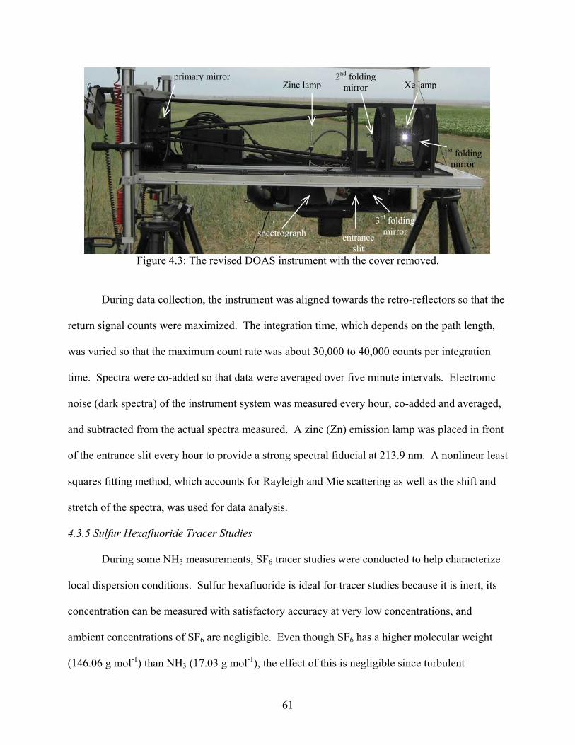
2nd folding mirror
primary mirror Zinc lamp Xe lamp
1st folding mirror
Figure 4.3: The revised DOAS instrument with the cover removed.
3rd folding mirror entrance
slit
spectrograph
During data collection, the instrument was aligned towards the retro-reflectors so that the
return signal counts were maximized. The integration time, which depends on the path length,
was varied so that the maximum count rate was about 30,000 to 40,000 counts per integration
time. Spectra were co-added so that data were averaged over five minute intervals. Electronic
noise (dark spectra) of the instrument system was measured every hour, co-added and averaged,
and subtracted from the actual spectra measured. A zinc (Zn) emission lamp was placed in front
of the entrance slit every hour to provide a strong spectral fiducial at 213.9 nm. A nonlinear least
squares fitting method, which accounts for Rayleigh and Mie scattering as well as the shift and
stretch of the spectra, was used for data analysis.
4.3.5 Sulfur Hexafluoride Tracer Studies
During some NH3 measurements, SF6 tracer studies were conducted to help characterize
local dispersion conditions. Sulfur hexafluoride is ideal for tracer studies because it is inert, its
concentration can be measured with satisfactory accuracy at very low concentrations, and
ambient concentrations of SF6 are negligible. Even though SF6 has a higher molecular weight
(146.06 g mol-1) than NH3 (17.03 g mol-1), the effect of this is negligible since turbulent
61

diffusion is the dominant transport mechanism (Kaharabata et al., 2000). Pure SF6 was released
from a single point at the center of the fields at rates ranging from ~0.6 to ~0.7 L min-1. Sulfur
hexafluoride concentrations were measured at several points along and beyond the DOAS
integration path using a Trace Gas Automated Profiling System (TGAPS) and portable syringe
samplers. The total length covered by the TGAPS sampling locations and syringe samplers was
greater than 800 m, which was typically long enough to capture background concentrations
outside of the plume. Continuous 5-minute average concentrations of SF6 were measured
through TGAPS sample lines at 7 locations. For more information on the TGAPS system, refer
to Flaherty et al. (2007). Programmable and battery-operated syringe samplers measured 30-
minute average SF6 concentrations. All samples were analyzed using a HP 5890 GC with an
ECD detector coupled with an electronic integrator (Benner and Lamb, 1985). Scott-Marrin
(Riverside, CA) SF6 standards with ±5% certified accuracy were used for calibration of the GC.
4.3.6 Inverse Gaussian Plume Model (SIMFLUX) for Estimating Ammonia Flux Rates
A Gaussian plume dispersion model (SIMFLUX) (Howard et al., 1996) was used in an
inverse approach to estimate NH3 emission rates. For fertigation periods, the sprinkler arm was
modeled as an array of point sources in a rectangular area (10 m by 400 m). For periods of no
fertigation or irrigation, the entire potato field was modeled as an array of point sources in a
circle (400 m radius). The DOAS measurement path was modeled as a line of point receptors.
All point sources and receptors were spaced 1 m apart. Measured variables, including wind
speed and wind direction, were input into the Gaussian plume equation. Analytical equations
(Martin, 1976) that represent the Pasquill-Gifford diffusion curves provided the best match for
the tracer studies conducted and, thus, were employed for estimating the vertical and horizontal
dispersion. The contributions from each point source were summed to estimate the concentration
62

at each downwind receptor. Ammonia flux rates were calculated from the average predicted
NH3 concentration based upon a point source release of 1 g s-1 point-1 and the measured DOAS
NH3 concentration.
A set of criteria was developed to determine which periods of NH3 measurements were
suitable for estimating NH3 flux rates using SIMFLUX. Only periods associated with wind
speeds greater than 1 m s-1, mean winds pointed towards the DOAS measurement path, wind
direction standard deviations less than 30 degrees, and measured NH3 concentrations greater than
the detection limit of 10 ppbv for 2008 and 5 ppbv for 2007 were used. For periods of low wind
speeds and high variation in wind direction, the theoretical basis of the Gaussian plume
dispersion model becomes invalid (see Figure C.16 in Appendix C for determination of cutoff
values).
Howard et al. (1996) discovered that significant errors result if a receptor is placed too far
crosswind from the plume centerline. As a result, only periods that captured a significant portion
of the NH3 plume were used for estimation of flux rates. For each measurement period,
SIMFLUX was used to determine the plume width along the extended DOAS measurement
position. The portion of the NH3 plume captured was calculated by determining the ratio of the
area of the plume measured and the area of the entire plume predicted.
4.3.7 Measuring Meteorological Variables
Meteorological information such as wind velocity and air temperature were measured
using a sonic anemometer at 10 Hz frequency located near the DOAS instrument. Soil moisture
and temperature were measured using Campbell Scientific Inc. CS515s Water Content
Reflectometers and copper/constantan thermocouples, respectively. Campbell Scientific CR10
data loggers were used to record data. Leaf stomatal conductance was measured using Decagon
63

Devices Hand Held Leaf Porometer. The water filled pore space (WFPS) was calculated as the
ratio of the volumetric water content and soil porosity.
4.4 RESULTS
4.4.1 Nitrous Oxide Flux Rates
The key factors affecting N2O emissions from the potato fields were soil WFPS, soil
temperature, and time after fertilizer application. Figure 4.4 is a plot of all measured N2O flux
rates as a function of time after the sprinkler has passed for irrigation and fertigation periods.
Individual plots for 7/17/07, 6/20/08, 6/21/08, and 7/22/08 (days when at least 4 hours of
sampling were conducted per chamber) can be found in Figures B.1, B.2, B.3, and B.4 in
Appendix B. As shown in Figure 4.4, N2O flux rates ranged from zero to 120 μg N2O m-2 s-1 and
from zero to 290 μg N2O m-2 s-1 immediately after irrigation and fertigation periods, respectively.
The average N2O flux rate for all measurements was 74 μg N2O m-2 s-1 with a standard deviation
of 73 μg N2O m-2 s-1 and a median of 55 μg N2O m-2 s-1. The average N2O flux rate after
fertigation was 97 μg N2O m-2 s-1 (standard deviation of 92 μg N2O m-2 s-1, median of 61 μg N2O
m-2 s-1). The average N2O flux rate after irrigation was 53 μg N2O m-2 s-1 (standard deviation of
42 μg N2O m-2 s-1, median of 45 μg N2O m-2 s-1). Generally N2O flux rates peaked between 2.5
to 3.5 hours after passing of the sprinkler arm. As expected, the maximum measured N2O flux
rate occurred during fertigation since the N inputs to the soil increased the amount of N available
for nitrification and denitrification.
64

300 300
250 250
200 200
150 150
100 100
50 50
0 0
N2O
Flu
x R
ate
(µg
m-2
s-1)
6
6
5
5
4
4
3
3
2
2
1
1
0
0
Time after sprinkler has passed (hrs)
7/09/07, chamber 1 fertigation 7/09/07, chamber 2 fertigation 7/11/07, chamber 4 fertigation 7/11/07, chamber 5 fertigation 7/11/07, chamber 6 fertigation 7/11/07, chamber 7 fertigation 7/11/07, chamber 8 fertigation 7/17/07, chamber 9 fertigation 6/20/08, chamber 10 irrigation 6/21/08, chamber 11 irrigation 6/21/08, chamber 12 irrigation 6/21/08, chamber 13 irrigation 7/22/08, chamber 14 fertigation
Figure 4.4: Nitrous oxide flux rates as a function of time after the sprinkler has passed (hrs) with water only (black) or water w/ N fertilizer (red).
Nitrous oxide flux rates as a function of soil surface temperature and soil WFPS are
plotted in Figures 4.5 and 4.6, respectively. The soil WFPS ranged from 68% to 87%, and soil
surface temperatures ranged from 14 °C to 29 °C. The greatest N2O flux rate occurred when the
soil surface temperature was 19 °C and the soil WFPS was 73%. Fertigation and irrigation
events combined with the ability of the fine-textured soil to hold water tightly resulted in
anaerobic soil conditions, thus allowing denitrification activity to occur. There was no clear
trend in N2O flux rates as a function of soil surface temperature since soil denitrifiers are adapted
to and capable of growing under a wide range of temperatures (Haverkort and MacKerron,
2000).
65

300 300
250 250
200 200
150 150
100 100
50 50
0 0
N2O
Flu
x R
ate
(µg
m-2
s-1)
28
28
26
26
24
24
22
22
20
20
18
18
16
16
14
14
Soil Surface Temperature (ºC)
7/09/07, chamber 1 fertigation 7/09/07, chamber 2 fertigation 7/11/07, chamber 4 fertigation 7/11/07, chamber 5 fertigation 7/11/07, chamber 6 fertigation 7/11/07, chamber 7 fertigation 7/11/07, chamber 8 fertigation 7/17/07, chamber 9 fertigation 6/20/08, chamber 10 irrigation 6/21/08, chamber 11 irrigation 6/21/08, chamber 12 irrigation 6/21/08, chamber 13 irrigation 7/22/08, chamber 14 fertigation
Figure 4.5: Nitrous oxide flux rates as a function of soil surface temperature. The gray and red data points represent periods of irrigation and fertigation, respectively.
300 300
250 250
200 200
150 150
100 100
50 50
0 0
N2O
Flu
x R
ate
(µg
m-2
s-1)
85
85
80
80
75
75
70
70
Water Filled Pore Space (%)
7/09/07, chamber 10 fertigation 7/09/07, chamber 12 fertigation 7/11/07, chamber 1 fertigation 7/11/07, chamber 6 fertigation 7/11/07, chamber 4 fertigation 7/11/07, chamber 7 fertigation 7/11/07, chamber 11 fertigation 7/17/07, chamber 9 fertigation 6/20/08, chamber 8 irrigation 6/21/08, chamber 4 irrigation 6/21/08, chamber 3 irrigation 6/21/08, chamber 2 irrigation 7/22/08, chamber 11 fertigation
Figure 4.6: Nitrous oxide flux rates as a function of soil WFPS. The black and red data points represent periods of irrigation and fertigation, respectively.
66

67
Table 4.3 contains N2O flux rates for fertigation periods with the corresponding fertilizer
application rate and the amount of N lost. The amount of N lost as a function of amount applied
ranged from zero to 12%, with a mean of 4%, which is comparable to documented emission
factor (EF) values of 0.1 to 8% (Dobbie and Smith, 2003). The standard deviation was 3.9% and
the median was 2.2%. Although denitrification activity was the main driver for observed N2O
fluxes, the bulk soil may not have been entirely anaerobic. Aerobic conditions may occur at the
base of the plants where it is less compacted.
Table 4.3: Percent of N lost for days of N fertilizer application
Date Chamber # Fertilizer App. Rate (μg N m-2 s-1)
N2O Flux Rate (μg N m-2 s-1) % N Lost
1 25 3.2 7/9/2007 2 24 3.1 4 92 11.8 5 68 8.8 6 45 5.8 7 0 0
7/11/2007
8
780
12 1.6 17 2.2 87 11.2 3.4 0.44 7/17/2007 9 780
3.4 0.44 16 1.3 19 1.7 32 2.7 7/22/2008 14 1170
20 1.7
4.4.2 Ammonia Concentrations
Measurements from 12:30 pm on 7/26/08 to 4:00 am on 7/27/08 (PDT) provide a good
example of measured NH3 concentrations. Figure 4.7 is a time-series plot of measured NH3
concentrations, wind speed, wind direction, air temperature, and soil temperature (measured 8
inches below the surface). Figures 4.8 to 4.9 are polar plots illustrating the measured NH3
concentrations as a function of sprinkler arm rotation angle (marked with circles) and wind
67

direction (marked with squares). Each polar plot shows the relationship between the location of
the sprinkler arm relative to the DOAS measurement path and the magnitude of the measured
NH3 concentrations. Additional time-series plots and polar plots for the rest of the data can be
found in Appendix C (Figures C.1 to C.15). Only NH3 concentrations above the DOAS
instrument detection limit (5 ppbv for 2007 and 10 ppbv for 2008) are shown in the polar plots.
160 160
120 120
80 80
40 40
0 0
NH
3 Con
c. (p
pbv)
2:00 PM7/26/2008
2:00 PM7/26/2008
4:00 PM
4:00 PM
6:00 PM
6:00 PM
8:00 PM
8:00 PM
10:00 PM
10:00 PM
12:00 AM7/27/2008
12:00 AM7/27/2008
2:00 AM
2:00 AM
4:00 AM
4:00 AM
Date and Time (PDT)
4
3
2
1
0
WS
(m/s
)
300
250
200
150
WD
(deg)
30 30
25 25
20 20
15 15 Tem
p. (C
)
Fertigation Error: 3 ppbv ± 30%
detection limit
ws wd
air soil surface
Figure 4.7: Time series plot of measured 30-minute average NH3 concentration, wind speed, wind direction, air temperature, and soil surface temperature from 07/26/08 12:30 pm to 07/27/08 4 am (PDT). The red line signifies the NH3 concentration detection limit of 10 ppbv. The bars on the wind direction data represent the 30-minute variation in wind direction (wind direction sigma).
From 12:30 pm to 5:30 pm on 7/26/08, the sprinkler arm was fertigating in the northwest
quadrant of the field and west/southwest winds were dominant (Figure 4.8). The average wind
speed was ~2.6 m s-1. Since the sprinkler arm was far from the DOAS measurement path, lower
68
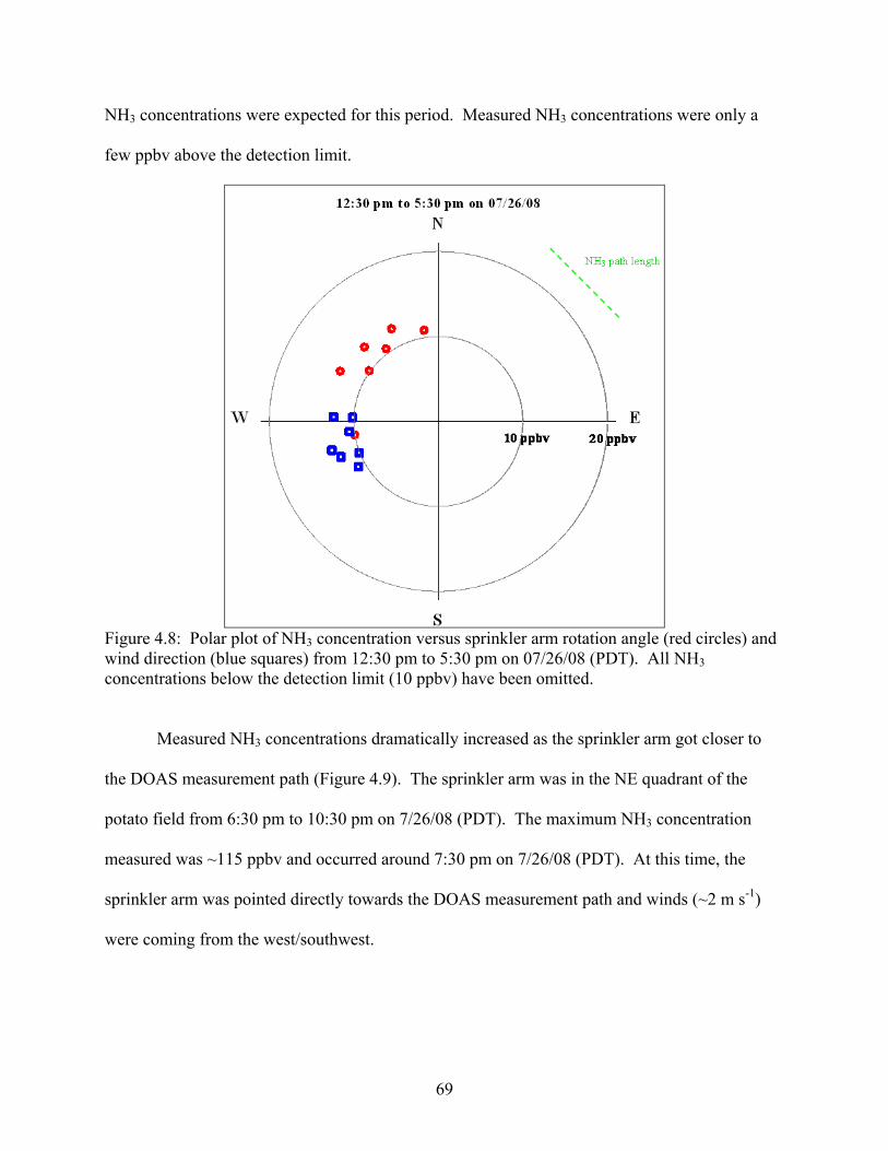
NH3 concentrations were expected for this period. Measured NH3 concentrations were only a
few ppbv above the detection limit.
Figure 4.8: Polar plot of NH3 concentration versus sprinkler arm rotation angle (red circles) and wind direction (blue squares) from 12:30 pm to 5:30 pm on 07/26/08 (PDT). All NH3 concentrations below the detection limit (10 ppbv) have been omitted.
Measured NH3 concentrations dramatically increased as the sprinkler arm got closer to
the DOAS measurement path (Figure 4.9). The sprinkler arm was in the NE quadrant of the
potato field from 6:30 pm to 10:30 pm on 7/26/08 (PDT). The maximum NH3 concentration
measured was ~115 ppbv and occurred around 7:30 pm on 7/26/08 (PDT). At this time, the
sprinkler arm was pointed directly towards the DOAS measurement path and winds (~2 m s-1)
were coming from the west/southwest.
69

Figure 4.9: Polar plot of NH3 concentration versus sprinkler arm rotation angle (red circles) and wind direction (blue squares) from 6 pm to 10:30 pm on 07/26/08 (PDT). All NH3 concentrations below the detection limit (10 ppbv) have been omitted.
Results show that NH3 concentrations (measured downwind of the potato field) depend
on sprinkler arm location, wind speed, and wind direction. The highest NH3 concentrations
measured in the summer of 2007 and the summer of 2008 were ~34 ppbv and ~112 ppbv,
respectively. Both peaks occurred during periods of fertigation with the sprinkler arm pointed
directly towards the DOAS measurement path and winds greater than 1 m s-1 were blowing
towards the DOAS measurement path. The field conditions for both days of peak NH3
measurements are summarized in Table 4.4. The large difference between the two maximum
values can be attributed to the greater rate of fertilizer application on 7/26/08 than on 7/18/07. In
addition, the measured peak on 7/26/08 occurred at night whereas the measured peak on 7/18/07
70

occurred during the day. During the day, unstable conditions dominate whereas during the night,
conditions are more stable and less mixing occurs.
Table 4.4: Field conditions for peak NH3 concentrations
Date/Time (PDT)
NH3 Conc. (ppbv)
N Fertilizer App. Rate
(μg NH3 m-2 s-1)
WS (m s-1)
WD (deg)
DOAS path location
Air Temp. (°C)
Soil Temp. (°C)
7/18/07, 12 pm ~34 950 ~3 240 NE quadrant 22.2 21.7
7/26/08, 7:30 pm ~110 1425 ~2 251 NE quadrant 27.2 20.4
The relationship between measured NH3 concentrations normalized by wind speed and
the sprinkler arm rotation angle during fertigation periods are shown in Figure 4.10. Only
measurements that were above the DOAS instrument detection limit and associated with wind
direction variations less than 30 degrees and wind speeds greater than 1.0 m s-1 are reported. As
expected, when the DOAS measurement path was positioned along the SE quadrant of the field,
the highest NH3 concentration was measured when the sprinkler arm rotation angle was 180°, or
due south. When the DOAS instrument was positioned along the NE quadrant of the field, the
highest NH3 concentration was measured when the sprinkler arm rotation angle was north-
northeast (25°).
71
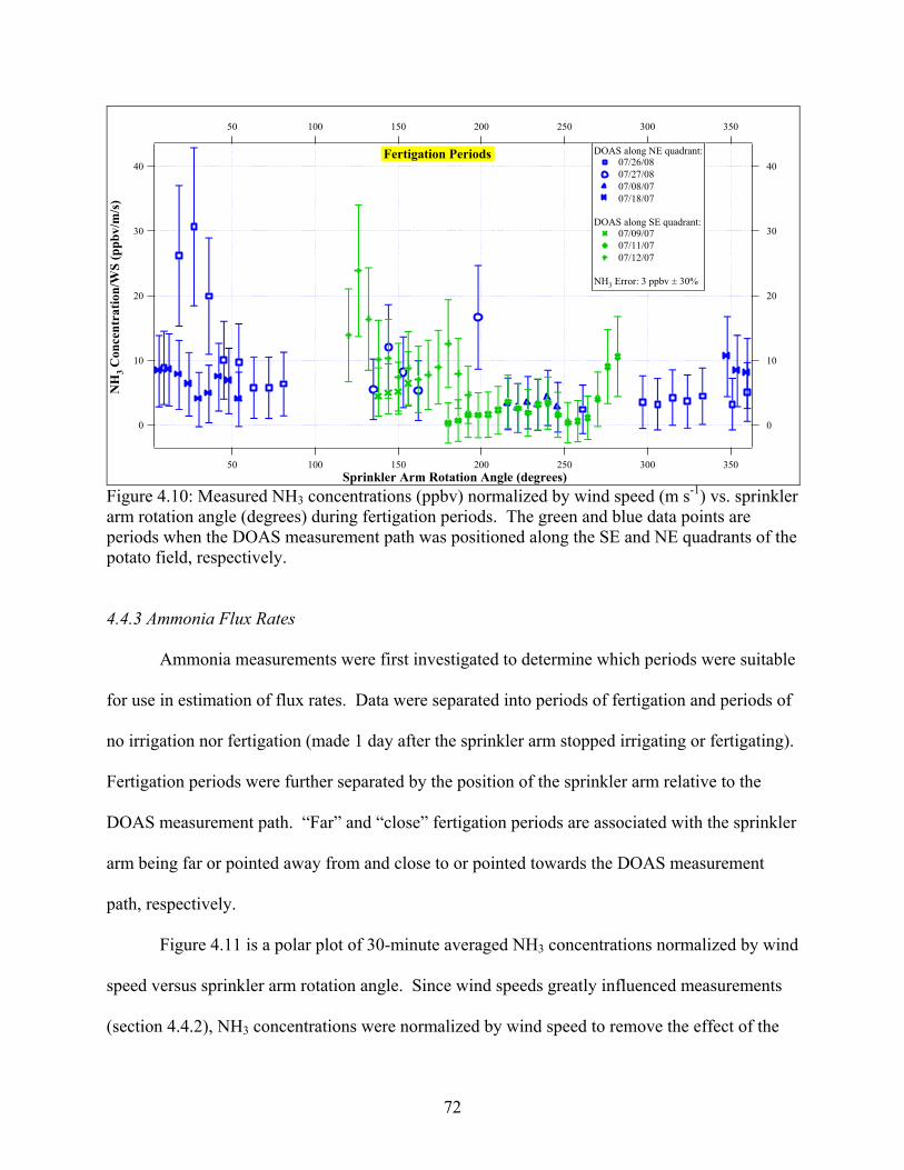
40 40
30 30
20 20
10 10
0 0
NH
3 Con
cent
ratio
n/W
S (p
pbv/
m/s
)
350
350
300
300
250
250
200
200
150
150
100
100
50
50
Sprinkler Arm Rotation Angle (degrees)
DOAS along NE quadrant: 07/26/08 07/27/08 07/08/07 07/18/07
DOAS along SE quadrant:
07/09/07 07/11/07 07/12/07
NH3 Error: 3 ppbv ± 30%
Fertigation Periods
Figure 4.10: Measured NH3 concentrations (ppbv) normalized by wind speed (m s-1) vs. sprinkler arm rotation angle (degrees) during fertigation periods. The green and blue data points are periods when the DOAS measurement path was positioned along the SE and NE quadrants of the potato field, respectively. 4.4.3 Ammonia Flux Rates
Ammonia measurements were first investigated to determine which periods were suitable
for use in estimation of flux rates. Data were separated into periods of fertigation and periods of
no irrigation nor fertigation (made 1 day after the sprinkler arm stopped irrigating or fertigating).
Fertigation periods were further separated by the position of the sprinkler arm relative to the
DOAS measurement path. “Far” and “close” fertigation periods are associated with the sprinkler
arm being far or pointed away from and close to or pointed towards the DOAS measurement
path, respectively.
Figure 4.11 is a polar plot of 30-minute averaged NH3 concentrations normalized by wind
speed versus sprinkler arm rotation angle. Since wind speeds greatly influenced measurements
(section 4.4.2), NH3 concentrations were normalized by wind speed to remove the effect of the
72

variable. Ammonia concentrations normalized by wind speed were generally greater for “close”
fertigation periods (4 ppbv m-1 s-1 to 11 ppbv m-1 s-1) than for “far” fertigation periods (1.7 ppbv
m-1 s-1 to 3.7 ppbv m-1 s-1). The difference between the two groups was expected since point
sources that were “close” to the DOAS measurement path dispersed less than “far” point sources.
The magnitudes of measured NH3 concentrations normalized by wind speed for periods of no
irrigation/fertigation were comparable to measurements made during “far” fertigation periods.
Figure 4.11: Polar plot of 30-min. averaged NH3 concentrations (ppbv) normalized by wind speed (m s-1) versus sprinkler arm rotation angle (degrees). Measurements made during “far” and “close” fertigation periods are in blue and red, respectively. Measurements made when the DOAS path was along the SE quadrant are marked as circles while measurements made when the DOAS path was along the NE quadrant are marked as x’s.
Fertigation Periods
73

74
Ammonia flux rates and percent NH3 loss as a function of wind speed during fertigation
periods and periods of fertigation/irrigation are plotted in Figures 4.12 and 4.13, respectively.
Similar to NH3 concentrations (section 4.4.2), NH3 flux rates and NH3 loss (ratio of NH3
emission rate to NH3 application rate) increased with increasing wind speed.
300
250
200
150
100
50
NH
3 Flu
x R
ate
(µg
m-2
s-1)
4.0
4.0
3.5
3.5
3.0
3.0
2.5
2.5
2.0
2.0
1.5
1.5
WS (m/s)
35
30
25
20
15
10
5
NH
3 Loss (%
)
NH3 Flux Rate, close NH3 Flux Rate, far NH3 loss, close NH3 loss, far
Fertigation Periods
Figure 4.12: NH3 flux rates (μg m-2 s-1) and NH3 loss (%) as a function of wind speed (m s-1) measured during fertigation periods.
74
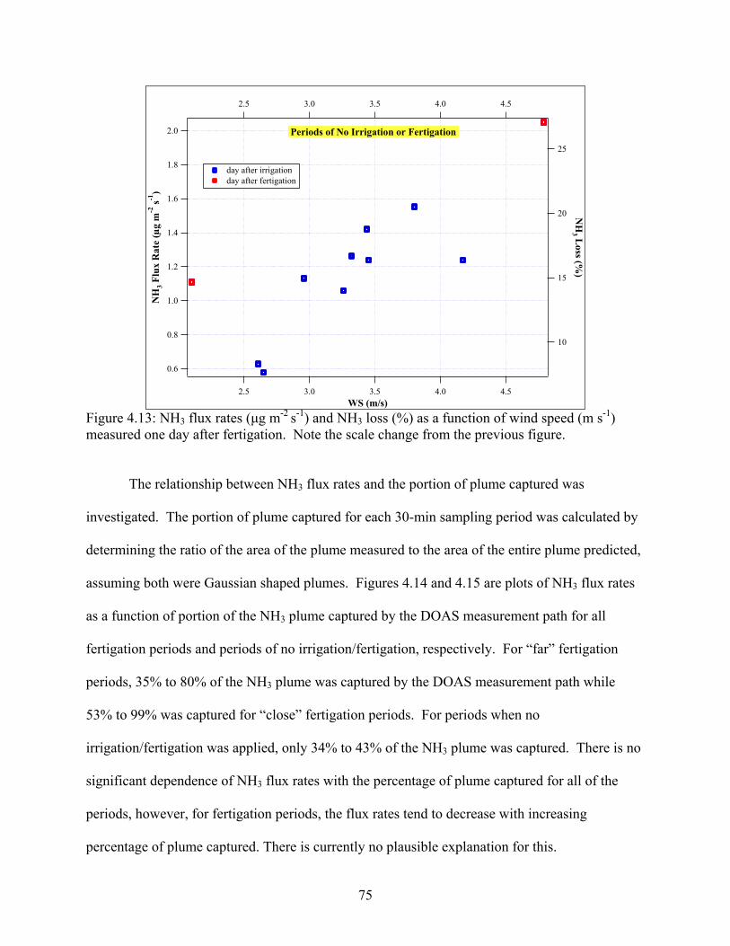
2.0
1.8
1.6
1.4
1.2
1.0
0.8
0.6
NH
3 Flu
x R
ate
(µg
m-2
s-1)
4.5
4.5
4.0
4.0
3.5
3.5
3.0
3.0
2.5
2.5
WS (m/s)
25
20
15
10
NH
3 Loss (%
)
Periods of No Irrigation or Fertigation
day after irrigation day after fertigation
Figure 4.13: NH3 flux rates (μg m-2 s-1) and NH3 loss (%) as a function of wind speed (m s-1) measured one day after fertigation. Note the scale change from the previous figure.
The relationship between NH3 flux rates and the portion of plume captured was
investigated. The portion of plume captured for each 30-min sampling period was calculated by
determining the ratio of the area of the plume measured to the area of the entire plume predicted,
assuming both were Gaussian shaped plumes. Figures 4.14 and 4.15 are plots of NH3 flux rates
as a function of portion of the NH3 plume captured by the DOAS measurement path for all
fertigation periods and periods of no irrigation/fertigation, respectively. For “far” fertigation
periods, 35% to 80% of the NH3 plume was captured by the DOAS measurement path while
53% to 99% was captured for “close” fertigation periods. For periods when no
irrigation/fertigation was applied, only 34% to 43% of the NH3 plume was captured. There is no
significant dependence of NH3 flux rates with the percentage of plume captured for all of the
periods, however, for fertigation periods, the flux rates tend to decrease with increasing
percentage of plume captured. There is currently no plausible explanation for this.
75

76
300 300
250 250
200 200
150 150
100 100
50 50
NH
3 Flu
x R
ate
(µg
m-2
s-1)
1.0
1.0
0.9
0.9
0.8
0.8
0.7
0.7
0.6
0.6
0.5
0.5
0.4
0.4
Portion of Plume Captured (%)
close far
Fertigation Periods
Figure 4.14: NH3 flux rates (μg m-2 s-1) as a function of the portion of plume captured (%) for fertigation periods.
2.0 2.0
1.8 1.8
1.6 1.6
1.4 1.4
1.2 1.2
1.0 1.0
0.8 0.8
0.6 0.6
NH
3 Flu
x R
ate
(µg
m-2
s-1)
0.42
0.42
0.40
0.40
0.38
0.38
0.36
0.36
0.34
0.34
Portion of Plume Captured (%)
Periods of No Irrigation or Fertigation
day after irrigation day after fertigation
Figure 4.15: NH3 flux rates (μg m-2 s-1) as a function of the portion of plume captured (%) for periods of no irrigation/fertigation.
76

Other variables were investigated to see if they impacted NH3 emission rates. The
relationship between NH3 flux rates and solar radiation, soil temperature, air temperature, and the
time after the sprinkler arm passed the DOAS measurement path were investigated and no
obvious trends were found. Periods used for estimation of NH3 flux rates occurred between 10
am and 6 pm (PDT), when fluctuations in air and soil temperatures were small. Due to the
limited range in air and soil temperatures, there was no obvious relationship between NH3
concentrations and emissions and soil and air temperatures (see Figures C.21 to C.24 in
Appendix C). For “far” fertigation periods, there was no dependence of NH3 flux rates with the
time after the sprinkler passed the DOAS measurement path (Figure 4.16).
25
20
15
10
5
NH
3 Los
s (%
)
8
8
6
6
4
4
2
2
Time after sprinkler arm has passed DOAS measurement path (hrs)
250
200
150
100
50
NH
3 Flux Rate (µg m
-2 s -1)
NH3 lossNH3 flux rate
"Far" Fertigation Periods
Figure 4.16: NH3 flux rates and percent loss as a function of time after the sprinkler passed the DOAS measurement path for “far” fertigation periods.
77

78
Table 4.5 shows the range of measured NH3 concentrations, estimated flux rates, and
percent of NH3 lost grouped by application status. The percent of NH3 lost was calculated by
dividing the estimated NH3 flux rate by the fertilizer application rate. There was no irrigation
period that met the criteria parameters and, thus, there are no calculations of flux rates and
percent of NH3 lost for irrigation periods. Estimated NH3 flux rates ranged from 34 μg NH3 m-2
s-1 to 250 μg NH3 m-2 s-1 and from 9.1 μg NH3 m-2 s-1 to 320 μg NH3 m-2 s-1 during fertigation
periods when the sprinkler arm was “far” and “close” to the DOAS measurement path,
respectively. Higher normalized NH3 concentrations were observed when the sprinkler arm was
closer to the DOAS path. However, in estimating the flux rates, dispersion is taken into account
and the variation in calculated flux rates is smaller. When there was no irrigation/fertigation,
NH3 flux rates varied from 0.6 μg NH3 m-2 s-1 to 2.1 μg NH3 m-2 s-1.
Table 4.5: Range of measured NH3 concentrations, estimated flux rates, and percent of NH3 loss grouped by application status.
Q (μg NH3 m-2 s-1) NH3 Loss (%) Application Status
Measured NH3 Conc. (ppbv) Min Average Max Min Avg. Max
No Irrigation or Fertigation 8.4 to 18.5 0.6 1.2 2.1 -- -- --
Fertigation (spray close to
DOAS) 9.9 to 34.0 9.1 80 320 0.95 8.5 34
Fertigation (spray far from
DOAS) 5.5 to 13.6 34 140 250 3.6 12.5 26.7
Ammonia loss during fertigation ranged from 0.95% to 48.4% (average of ~8% for “far”
periods and ~12% for “close” periods). The frequency distribution of NH3 flux rates during
fertigation are shown in Figure 4.17. The average NH3 flux rate during all fertigation periods
was 100 μg m-2 s-1. The standard deviation was ~84 μg m-2 s-1 and the median was ~75 μg m-2 s-1.
78

79
8 8
6 6
4 4
2 2
0 0
Fre
quen
cy
300
300
250
250
200
200
150
150
100
100
50
50
0
0
NH3 Flux Rate (µg m-2 s-1)
Fertigation Periods
Figure 4.17: Frequency distribution of NH3 flux rates during fertigation periods.
A total N loss of 47% was estimated for the entire period of heavy N fertigation (month of July).
A total of 38% was lost through NH3 emissions. For N lost as NH3, the following assumptions
were used:
• an average of 2.75 Mg of N (6050 lbs) total was applied to the potato fields
• the average NH3 flux during irrigation was assumed to be 50% of the average NH3 flux
during fertigation
• the average NH3 flux during periods of no irrigation nor fertigation was 1 μg m-2 s-1
• daytime and nighttime flux rates are the same, even though flux rates were only
calculated from daytime measurements
• the emissions during irrigation and fertigation were based on the 400 m by 10 m area
underneath the sprinkler arm
• the emissions during periods with no irrigation nor fertigation were constant throughout
the month (the decrease of emissions with time after fertigation was not accounted for).
79

80
Of the 38% N lost through NH3 emissions, 27% of the applied N was lost during periods of no
fertigation/irrigation while 8% was lost during fertigation and 3% was lost during irrigation.
More was lost during no irrigation/fertigation periods than fertigation or irrigation periods
because of the greater time period and area of emissions used for that calculation.
Table 4.6: Total N Loss through NH3 Emissions for the month of July.
Application Status
# Hours
Avg. Emission Rate (Q)
(μg-NH3 m-2 s-1)
Avg. Q (μg-N m-2 s-1)
July N loss
(kg-N)
% of Lost N (NH3
Emissions) No Fertigation nor Irrigation 414 1.2 1 749 27%
Fertigation 180 100 84 218 8% Irrigation 150 50 42 91 3%
Total 38%
A total of 9% was lost through N2O emissions. For N lost as N2O the following assumptions
were used:
• an average of 2.75 Mg of N (6050 lbs) total was applied to the potato fields
• the average N2O flux after irrigation was assumed to be 100 μg N2O m-2 s-1
• the average N2O flux after fertigation was assumed to be 50 μg N2O m-2 s-1
• N2O flux rates on days of no irrigation nor fertigation were assumed negligible
• emission rates were assumed constant (no decrease with time)
Of the 9% N lost through N2O emissions, 6% of the applied N was lost during fertigation and 3%
was lost during irrigation.
80

81
Table 4.7: Total N Loss through N2O Emissions for the month of July.
Application Status
# Hours
Avg. Emission Rate (Q)
(μg-N2O m-2 s-1)
Avg. Q (μg-N m-2 s-1)
July N loss (kg-N)
% of Lost N (N2O
Emissions) No Fertigation nor Irrigation 414 0 0 0 0%
Fertigation 180 100 32 174 6% Irrigation 150 50 16 72 3%
Total 9%
4.5 Conclusions
Ammonia results show that as wind speeds increased, so did the measured NH3
concentrations as well as estimated NH3 flux rates and percent of NH3 loss. Wind direction
influenced measured NH3 concentrations and, as a result, calculated flux rates for periods when
winds blew towards the DOAS measurement path more accurately represent emission rates from
the potato fields. There were no clear relationships between NH3 emissions and solar radiation,
soil and air temperature, and time after the sprinkler arm passed the DOAS measurement path.
Estimated NH3 flux rates ranged from 9.1 μg NH3 m-2 s-1 to 460 μg NH3 m-2 s-1 for
fertigation periods (average 100 μg NH3 m-2 s-1) and from 0.6 μg NH3 m-2 s-1 to 2.1 μg NH3 m-2 s-1
(average 1.2 μg NH3 m-2 s-1) for periods of no irrigation/fertigation which indicates that a
significant fraction of NH3 loss from these fields occurs as a result of direct volatilization of NH3
during fertigation. The estimated NH3 flux rates from this study are much higher than the
standard rate of 0.01 μg NH3 m-2 s-1 typically used for all crops when compiling global emission
inventories (Bouwman et al., 1997), with the flux rate obviously dependent upon quantity of
applied N. The amount of NH3 loss ranged from 0.95% to 48% for fertigation periods (average
10%), which is comparable to reported NH3 loss from other studies (range from 8 to 18% using
micrometeorological methods and from zero to 45% using dynamic flow chambers) (IFA, 2001).
81
A total N loss of 47% was estimated for the entire period of heavy N fertigation (month
of July). Of the 47% N lost, 38% was lost through NH3 emissions and 9% was lost through N2O
emissions. Previous studies available in literature report similar total N loss in potato plants.
Reported N loss under current best management practices has been reported to be ~35% of N
applied (Lang et al., 1999) with a mean of 60% (Balasubramanian et al., 2004).
Nitrous oxide flux rates generally peaked between 2.5 and 3.5 hours after irrigation or
fertigation and appeared to be a result of denitrification activity (soil WFPS ranged from 68% to
87%). Nitrous oxide flux rates ranged from negligible to 280 μg N2O m-2 s-1 and are much
higher than reported emission rates by Flessa et al. (2002), who reported mean N2O emissions of
0.02 and 0.03 μg N2O m-2 s-1 during the 1997 and 1998 growing periods of two adjacent potato
fields in Germany using automated gas sampling chambers.
The average N loss as N2O ranged from zero to 12% (average ~4%) of the applied N
fertilizer which is comparable to documented EF values of 0.1 to 8% (Dobbie and Smith, 2003).
The average N loss is much higher than that reported by Haile-Mariam et al. (2008), who
reported N2O losses of 0.3% of applied fertilizer in potato fields in central Washington during
the 2005 and 2006 growing seasons using static chambers. Similar to the fields used in this
study, the fields used by Haile-Mariam et al. (2008) were applied with UAN solution 32 through
a center pivot irrigation system and aerobic soil conditions dominated in the fields.
82
CHAPTER 5
ERROR ANALYSIS
5.1 Uncertainties in NH3 Measurements
There are various errors associated with the measurements of NH3. Uncertainty in NH3
measurements result from errors in the absolute NH3 absorption cross section of ±20% (Mount et
al., 2002). The error in residual analysis was approximately ±25% and was due to uncontrollable
variations in the dark current (electronic noise of the system) caused by the external radiator used
for temperature regulation of the CCD detector, which resulted in difficult subtraction of darks
during data analysis. Other errors include changes in the spectral output of the Xe lamp which
could not be monitored at high frequency and illumination problems on the system optics from
atmospheric turbulence. The overall error in the NH3 concentration data combining all of these
uncertainties in quadrature is estimated to be ± 30% ± 3ppbv.
5.2 Uncertainties in NH3 Flux Rates
The uncertainty in estimated NH3 emission rates result from errors associated with the
estimation of NH3 concentrations as well as errors in SIMFLUX. SIMFLUX assumes uniform
emission rates from all of the point sources within the field. Numerous factors (i.e.
environmental factors, soil properties) regulate NH3 loss from the soil and potato plants and
these factors may not have been uniform throughout the field. During fertigation periods, only
the area covered by the sprinkler arm was modeled (400 m by 10 m) as an NH3 source. While
other parts of the field contributed to NH3 emissions, it was difficult to differentiate between
direct volatilization from the spray of the sprinkler arm and the entire field.
83

There are also errors associated with the SF6 tracer data used to calibrate the dispersion
algorithm in SIMFLUX. During SF6 tracer studies, the sources of error include changes in the
SF6 release rate, GC analysis (uncertainty in the gas standards ±5%), and error in duplicates.
When compared with the SF6 tracer studies, the equations by Martin (1976) for determining
dispersion coefficients resulted in an average mean normalized gross error (MNGE) of 41%
between predicted and observed SF6 concentrations (Appendix A). The error in the NH3 flux
estimates is approximately ± 52%.
5.3 Uncertainties in N2O Measurements
The uncertainty in N2O measurements are derived from errors in chamber sampling and
GC analysis. Errors associated with the GC analysis include the uncertainty in the gas standard
utilized for the calibration of the voltage signal from the ECD (±10%) and the error in duplicate
measurements (maximum error was ±18%). The total error ranged from ±11% to ±21%.
The errors associated with the chamber sampling cannot be quantified and include the
uncertainty in the accuracy of volume measurements inside the chambers since soil surfaces
were irregular. In addition, the concentration with time data was noisy and determination of flux
rates required disregarding outliers based on judgment. Also, the number of measurements
collected was not enough to capture the heterogeneity of N2O emissions throughout the field.
Other errors associated with chamber sampling should be minimal since installation and
sampling of chambers were conducted according to the prudent guidelines of the USDA-ARS
GRACEnet protocols (USDA-ARS, 2003). All samples were analyzed within a day of collection
to prevent error due to leakage and approximately 10% of all the samples were reanalyzed during
each analytical period to ensure data quality.
84

85
CHAPTER 6
CONCLUSIONS AND FUTURE WORK
There are limited studies that have measured the magnitude of Nitrogen (N) emissions
from intensively managed croplands. It is important to understand the magnitude and factors
controlling NH3 and N2O emissions because they pose negative effects to human health and the
environment. In this research, concentrations and fluxes of ammonia (NH3) and (N2O) from
potato fields in central Washington were measured during the 2007 and 2008 growing seasons
(June – August).
Nitrous oxide fluxes were measured using a static chamber method and samples were
analyzed using a GC-ECD. The chamber method was useful for investigating the processes
controlling N2O fluxes. However, the method made it difficult to extrapolate measured fluxes to
field-scale estimates since there is a wide range of environmental conditions throughout the
fields as well as a large variation in the soil properties.
This study is the first field experiment using the DOAS technique to measure NH3 fluxes
from potato fields. The DOAS technique proved to be an appropriate method for measuring NH3
flux rates from the fields because it did not disturb the soil-plant-atmosphere pathway and it
provided measurements integrated over a large area. However, NH3 measurements were limited
by the problems associated with the revised instrument (i.e. misalignment of mirrors, inability of
the internal cooler within the CCD detector to regulate temperature), which disrupted data
collection and decreased data quality. Correction of those problems will significantly enhance
future measurements made by DOAS.

86
Suggested Future Work:
• Further improvement of the DOAS instrument (i.e. re-aligning of the mirrors, addition of
an appropriate cooler to regulate temperature for the CCD detector) will improve future
measurement quality and quantity.
• Measurements of NH3 and other factors influencing emissions need to be made over a
sufficiently longer time period so that the relationships between NH3 emissions and
influencing factors can be determined.
• The use of a relaxed-eddy accumulation technique (REA) concurrent with the DOAS
technique would allow for continuous NH3 flux measurements and provide
complementary data to the current data set. (Zhu et al. (2000) have shown that the REA
technique is successful in measuring NH3 fluxes over a corn field.)
• Measurement of emissions from other potato fields under a different management
practice. (The fields used in this study were continuously applied with small amounts of
N fertilizer throughout the growing season. Other farmers apply large amounts of N
fertilizer at one time only (i.e. at the beginning of the season)).
• Use of an automated system of chambers, which would allow for continuous, long-term
measurements of N2O and provide a better understanding of spatial and temporal
variations in N2O fluxes throughout the fields.
86

REFERENCES
Arya, S.P., 1999. Air Pollution Micrometeorology and Dispersion. Oxford University Press, Inc., New York, New York.
Balasubramanian, V., Alves, B., Aulakh, M., Bekunda, M., Cai, Z., Drinkwater, L., Mugendi, D.,
van Kessel, C., Oenema, O., 2004. Crop, Environmental, and Management Factors Affecting Nitrogen Use Efficiency. In: A. Mosier, J. Syers, J. Freney (eds.) Agriculture and the Nitrogen Cycle: Assessing the Impacts of Fertilizer Use on Food Production and the Environment. 19-33. Island Press, Washington.
Benner, R. L., Lamb, B. 1985. A fast response continuous analyzer for halogenated atmospheric
tracers. Journal of Atmospheric Oceanic Technology 2, 582–589. Bouwman, A.F., 1996. Direct Emission of Nitrous Oxide from Agricultural Soils. Nutrient
Cycling in Agroecosystems 46, 53-70. Bouwman, A.F., Lee, D.S., Asman, W.A.H., Dentener, F.J., Van Der Hoek, K.W., Olivier,
J.G.J., 1997. A global high-resolution emission inventory for ammonia. Global Biogeochemical Cycles 11(4), 561-587.
Bouwman, A.F., Boumans, L.J., 2002. Estimation of Global NH3 Volatilization Loss from
Synthetic Fertilizers and Animal Manure Applied to Arable Lands and Grasslands. Global Biogeochemical Cycles 16 (2), 8-1 to 8-15.
Briggs, G., 1973. Diffuion Estimation for Small Emissions, ATDL Contribution File No. 79,
Atmospheric Turbulence and Diffusion Laboratory. Chen, J., Vaughan, J. , Avise, J., O'Neill, S., Lamb, B., 2008. Enhancement and evaluation of the
AIRPACT ozone and PM2.5 forecast system for the Pacific Northwest. Journal of Geophysical Research 113, D14305, doi:10.1029/2007JD009554.
Christensen, S., Ambus, P., Arah, J.R.M., Clayton, H., Galle, B., Griffith, D. W. T., Hargreaves,
K. J., Klenzedtsson, L., Lind, A., Maag, M., Scott, A., Skiba, U., Smith, K. A., Welling, M., Wienhold, F. G., 1996. Nitrous oxide emission from an agricultural field: Comparison between measurements by flux chamber and micrometerological techniques. Atmospheric Environment 30 (24), 4183-4190.
Dobbie, K.E., McTaggart, I.P., Smith, K,A., 1999. Nitrous Oxide Emissions from Intensive
Agricultural Systems: Variations between Crops and Seasons, Key Driving Variables, and Mean Emission Factors. Journal of Geophysical Research-Atmospheres 104, 26891-26899.
Dobbie, K.E., Smith, K.A., 2003. Nitrous oxide emission factors for agricultural soils in Great
Britain: the impact of soil water-filled pore space and other controlling variables. Global Change Biology 9, 204-218.
87
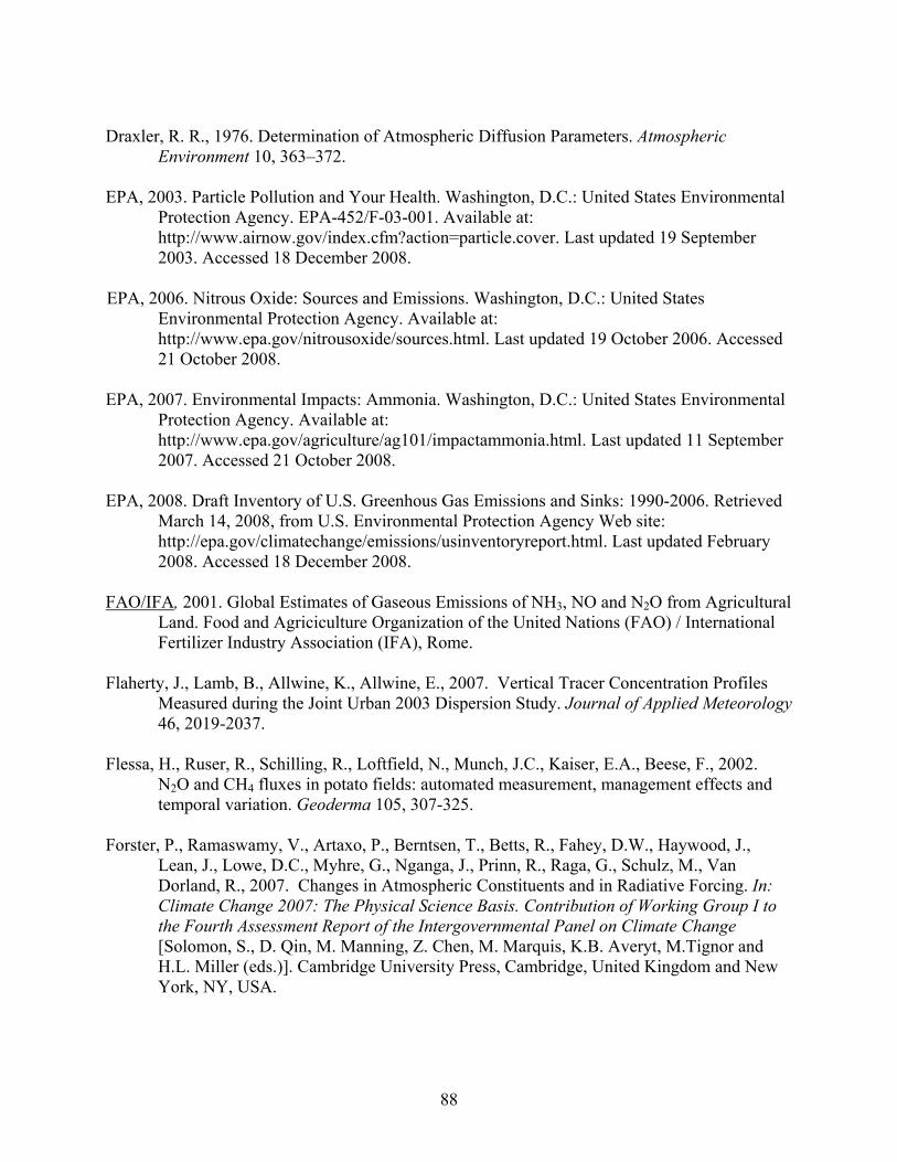
88
Draxler, R. R., 1976. Determination of Atmospheric Diffusion Parameters. Atmospheric
Environment 10, 363–372. EPA, 2003. Particle Pollution and Your Health. Washington, D.C.: United States Environmental
Protection Agency. EPA-452/F-03-001. Available at: http://www.airnow.gov/index.cfm?action=particle.cover. Last updated 19 September 2003. Accessed 18 December 2008.
EPA, 2006. Nitrous Oxide: Sources and Emissions. Washington, D.C.: United States
Environmental Protection Agency. Available at: http://www.epa.gov/nitrousoxide/sources.html. Last updated 19 October 2006. Accessed 21 October 2008.
EPA, 2007. Environmental Impacts: Ammonia. Washington, D.C.: United States Environmental
Protection Agency. Available at: http://www.epa.gov/agriculture/ag101/impactammonia.html. Last updated 11 September 2007. Accessed 21 October 2008.
EPA, 2008. Draft Inventory of U.S. Greenhous Gas Emissions and Sinks: 1990-2006. Retrieved
March 14, 2008, from U.S. Environmental Protection Agency Web site: http://epa.gov/climatechange/emissions/usinventoryreport.html. Last updated February 2008. Accessed 18 December 2008.
FAO/IFA, 2001. Global Estimates of Gaseous Emissions of NH3, NO and N2O from Agricultural
Land. Food and Agriciculture Organization of the United Nations (FAO) / International Fertilizer Industry Association (IFA), Rome.
Flaherty, J., Lamb, B., Allwine, K., Allwine, E., 2007. Vertical Tracer Concentration Profiles
Measured during the Joint Urban 2003 Dispersion Study. Journal of Applied Meteorology 46, 2019-2037.
Flessa, H., Ruser, R., Schilling, R., Loftfield, N., Munch, J.C., Kaiser, E.A., Beese, F., 2002.
N2O and CH4 fluxes in potato fields: automated measurement, management effects and temporal variation. Geoderma 105, 307-325.
Forster, P., Ramaswamy, V., Artaxo, P., Berntsen, T., Betts, R., Fahey, D.W., Haywood, J.,
Lean, J., Lowe, D.C., Myhre, G., Nganga, J., Prinn, R., Raga, G., Schulz, M., Van Dorland, R., 2007. Changes in Atmospheric Constituents and in Radiative Forcing. In: Climate Change 2007: The Physical Science Basis. Contribution of Working Group I to the Fourth Assessment Report of the Intergovernmental Panel on Climate Change [Solomon, S., D. Qin, M. Manning, Z. Chen, M. Marquis, K.B. Averyt, M.Tignor and H.L. Miller (eds.)]. Cambridge University Press, Cambridge, United Kingdom and New York, NY, USA.

Freney, J.R., Simpson, J.R., 1983. Gaseous Loss of Nitrogen from Plant-Soil Systems. Martinus Nijhoff/Dr. W. Junk Publishers, The Hague, Netherlands.
Galloway, J.N., Dentener, F.J., Capone, D.G., Boyer, E.W., Howarth, R.W., Seitzinger, S.P.,
Asner, G.P., Cleveland, C.C., Green, P.A., Holland, E.A., Karl, D.M., Michaels, A.F., Porter, J.H., Townsend, A.R., Vorosmarty, C.J., 2004. Nitrogen cycles: Past, present and future. Biogeochemistry 70, 153-226.
Haile-Mariam, S., Collins, H. P., Higgins, S. S., 2008. Greenhouse Trace Gas Fluxes from an
Irrigated Sweet Corn (Zea mays L.) - Potato (Solanum tuberosum L.) Rotation. Journal of Environmental Quality 37, 759-771. DOI: 10.2134/jeq2007.0400
Hanna, S.R., Briggs, G.A., Hosker, R.P., 1982. Handbook on Atmospheric Diffusion.
DOE/TIC11223, Tech. Information Center, U.S. Dept. of Energy, Oak Ridge, TN Department of Energy, 102. [NTIS DE8-2002-045.]
Haverkort, A.J., MacKerron, D.K.L., 2000. Recommendations and trends in research and
practice of application of nitrogen and water to potato crops. In: Haverkort, A.J. & D.K.L. MacKerron (Eds.), Management of nitrogen and water in potato production. Wageningen Pers, Wageningen, 301-310.
Hutchinson, G.L., Mosier, A.R., 1981. Improved soil cover method for field measurements of
nitrous oxide fluxes. Soil Science Society of America Journal 45, 311–316. IPCC (Intergovernmental Panel on Climate Change). Climate Change 1995. Impacts,
Adaptations and Mitigation of Climate Change: Scientific–Technical Analyses; Watson, R.T., Zinyowera, M.C., Moss, R.H., Eds.; Cambridge University Press: Cambridge, England, 1996; 1–878.
Kaharabata, S.K., Schuepp, P.H., 2000. Estimating Methane Emissions from Dairy Cattle
Housed in a Barn and Feedlot using an Atmospheric Tracer. Environmental Science & Technology 34 (15), 3296-3302.
Krasnec, J., Demaray, D., Lamb, B., Benner, R., 1984. Automated sequential syringe sampler for
atmospheric tracer studies. Journal of Atmospheric and Oceanic Technology 1, 372-376. Lang, N.S., Stevens, R.G., Thornton, R.E., Pan, W.L., Victory, S., 1999. Irrigated potato nutrient
management guide for central Washington. WSU Extension Bulletin #241. Liu, G., Li, Y., Alva, A.K., 2007. Temperature quotients of ammonia emission of different
nitrogen sources applied to four agricultural soils. Soil Science Society of America Journal 71, 1482-1489.
89

Livingston, G.P., Hutchinson, G.L., 1995. Enclosure-based measurement of trace gas exchange: applications and sources of error. In. P.A. Matson and R.C. Harriss (eds.) Biogenic Trace Gases: Measuring Emissions from Soil and Water. Methods in Ecology. 14-51. Blackwell Science Cambridge University Press, London.
Martin, D.O., 1976. The change of concentration standard deviation with distance, Journal of Air
Pollution Control Association 2, 26. McGinn, S.M., Janzen, H.H., 1997. Ammonia Sources in Agriculture and their Measurement.
Canadian Journal of Soil Science 78, 139–148. Mohan, M., Siddiqui, T.A., 1997. An Evaluation of Dispersion Coefficients for Use in
Air Quality Models. Boundary Layer Meteorology 84, 177-206.
Mount, G.H., Rumburg, B., Havig, J., Lamb, B., Westberg, H., Yonge, D., Johnson, K., Kinciad, R., 2002. Measurement of atmopsheric ammonia at a dairy using differential optical absorption spectroscopy in the mid-ultraviolet. Atmospheric Environment 36, 1799-1810.
Pandis, S.N., Wexler, A.S., Seinfiekld, J.H., 1995. Dynamics of Tropospheric Aerosols. Journal
of Physical Chemistry 99 (24), 9646-9659. DOI: 10.1021/j100024a003 Poole, C.F., Poole, S.K., 1991. Chromatography Today. Elsevier Scientific. Amsterdam, The
Netherlands. Potter, C., Krauter, C., Klooster, S., 2001. Statewide Inventory Estimates of Ammonia Emissions
From Fertilizer Applications in California. Project report to California Air Resources Board, Sacramento, CA. Contract# ID98-76.
Rumburg, B., Mount, G., Yonge, D., Lamb, B., Westberg, H., Filipy, J., Bays, J., Kincaid, R.,
Johnson, K., 2006. Atmospheric flux of ammonia from sprinkler application of dairy waste. Atmospheric Environment 40, 7246-7258.
Seinfeld, J.H., Pandis, S.N., 1998. Atmospheric chemistry and physics: from air pollution to
climate change. Wiley-Interscience. USA. Smith, K.A., McTaggart, I.P., Tsuruta, H., 1997. Emissions of N2O and NO Associated with
nitrogen fertilization in intensive agriculture, and the potential for mitigation. Soil Use and Management 13, 296-304.
Sommer, S.G., Schjoerring, J.K., Denmead, O.T., 2004. Ammonia emission from mineral
fertilizers and fertilized crops. Advances in Agronomy 82, 557-622. Stockle, C., Martin, S., Campbell, G., 1994. CropSyst, a cropping systems simulation model:
Water/nitrogen budgets and crop yield. Agricultural Systems 46, 335-359.
90

91
Sutton MA., Schjoerring, J.K., Wyers, G.P., Duyzer, J.H., Ineson, P., Powlson, D.S., 1995. Plant-atmosphere exchange of ammonia. Philosophical Transactions: Physical Sciences and Engineering 351 (1696), 261-278.
Turnipseed, A., Pressley, S., Karl, T., Lamb, B., Nemitz, E., Allwine, G., Cooper, W., Shertz, S.,
Guenther, A., 2008. The use of disjunct eddy sampling methods for the determination of ecosystem level fluxes of trace gases. Atmospheric Chemistry and Physics Discussions 8, 13413-13451.
USDA-ARS GRACEnet, 2003. Chamber-based Trace Gas Flux Measurement Protocol. U.S.
Department of Agriculture- Agricultural Research Service GRACEnet. Available at: http://gracenet.usda.gov/GRACEnetTraceGasProtocol.pdf. 24 April 2003.
Vitousek, P.M., Aber, J.D., Howarth, G.E., Likens, G.E., Watson, P.A., Schindler, D.W.,
Schlesinger, W.H., Tilman, D.W., 1997. Human alterations of the global nitrogen cycle: sources and consequences. Ecological Applications, 7, 737-750.
Vitousek, P.M., Aber, J.D., Howarth, G.E., Likens, G.E., Watson, P.A., Schindler, D.W.,
Schlesinger, W.H., Tilman, D.W., 2000. Human alterations of the global nitrogen cycle: Causes and consequences. Human Alteration of the Global Nitrogen Cycle http://esa.sdsc.edu/tilman.html
Zhu, T., Pattey, E., Desjardins, R.L., 2000. Relaxed Eddy-Accumulation Technique for
Measuring Ammonia Volatilization. Environmental Science & Technology. 34, 199-203. DOI: 10.1021/es980928

APPENDIX A:
COMPARISON OF VARIOUS METHODS
FOR DETERMINING DISPERSION COEFFICIENTS
92

In this appendix, a brief overview of the various methods for determining the dispersion
coefficients and the comparison results are presented.
A.1 Description of Sigma Methods
Critical input parameters to the Gaussian diffusion models are the dispersion coefficients
(σy and σz), which express the spread of the plume in the horizontal and vertical crosswind
directions. These coefficients can be determined empirically or theoretically. The methods
compared were:
1) Empirical methods:
i) Martin’s equations based on Pasquill-Gifford diffusion curves (Martin, 1976)
ii) Briggs’ equations for open-country conditions based on several field studies (Briggs,
1973)
2) Theoretical method: Taylor’s near-field dispersion theory (Mohan and Siddiqui, 1997)
3) Combination of theory and empirical results: Draxler’s method (Draxler, 1976)
A.1.1 Empirical Methods
Values of σy and σz may be obtained from empirical results. Perhaps the most well-
known diffusion study is the 1956 Project Prairie Grass in O’Neill, Nebraska. During Project
Prairie Grass, sulfur dioxide (SO2) was used as the tracer gas and released at a height of 0.5 m
above ground over a large flat field (Arya, 1999). Concentrations at 1.5 m above ground were
measured at distances between 50 and 800 m from the source and were based on 10 min
sampling periods (Arya, 1992). This experiment resulted in the Pasquill and Gifford (P–G)
dispersion curves. To estimate σy and σz from the P-G curves, the stability class must first be
determined based on simple measurements such as sunshine, cloud cover, and wind speed
93

measured at 10 meters above ground, as shown in Table 3.2. “Strong” incoming solar radiation
corresponds to a solar angle greater than 60° with clear skies, while “slight” incoming solar
radiation corresponds to a solar angle less than 35° with clear skies (Arya, 1999). Along with
solar angle, cloud cover is also considered when determining the strength of incoming solar
radiation. The use of computers for solving the Gaussian dispersion equations make it desirable
to convert the P-G curves into analytical equations. The equations of Martin (1976) represent a
reasonable fit to the Pasquill and Gifford (P–G) dispersion curves.
Table A.1: Pasquill Stability Classes
Surface Wind Speed Daytime Incoming Solar Radiation
Nighttime Cloud Cover
(m s-1) Strong Moderate Slight > 50% < 50% < 2 A A-B B E F 2-3 A-B B C E F 3-5 B B-C C D E 5-6 C C-D D D D > 6 C D D D D
Note: Class D applies to heavily overcast skies, at any wind speed day or night
The following equations were developed by Martin for calculating the dispersion
coefficients:
894.0axy =σ A.1
fcxdz +=σ A.2
where the constants a, c, d, and f are given in Table A.2. The values of σy and σz are in meters
when the value of the downwind distance x of the receptor from the source is given in
kilometers.
94

Table A.2: Values of a, c, d, and f for use in Martin’s equation x < 1 km x > 1 km
Stability a c d f c d f
A 213 440.8 1.041 9.27 459.7 2.094 -9.6 B 156 106.6 1.149 3.3 108.2 1.098 2.0 C 104 61.0 0.911 0.0 61.0 0.911 0.0 D 68 33.2 0.725 -1.7 44.5 0.516 -13.0 E 50.5 22.8 0.675 -1.3 55.4 0.305 -34.0 F 34 14.35 0.740 -0.35 62.6 0.180 -48.6
In addition to Project Prairie Grass, a number of other diffusion experiments have been
conducted to empirically estimate the dispersion coefficients. For rural situations, the three main
diffusion experiments are the 1956 Project Prairie Grass, the Brookhaven National Laboratory
(BNL) experiments, and the Tennessee Valley Authority (TVA) experiment. Results from
Project Prairie Grass are for non-buoyant, near ground level releases at downwind distances less
than 1km. The BNL experiment results reflect effects of elevated releases (~108 m above
ground) over a rougher surface at downwind distances extending to tens of kilometers (Arya,
1999). The TVA results reflect effects of highly buoyant releases from higher elevations over
gently rolling terrain (Arya, 1999). In 1973, Briggs synthesized the results from Project Prairie
Grass, BNL, and TVA to produce a set of formulas for open country situations, which are shown
in Table A.3 (Arya, 1999). Briggs’ formulas use the Pasquill stability classes.
Table A.3: Briggs’ (1973) Interpolation Formulas for Open Country Stability σy (m) σz (m)
A 0.22x(1 + 0.0001x)-.5 .20x B 0.16x(1 + 0.0001x)-.5 .12x C 0.11x(1 + 0.0001x)-.5 .08x(1 + 0.0002x)-.5 D 0.08x(1 + 0.0001x)-.5 .06x(1 + 0.0015x)-.5 E 0.06x(1 + 0.0001x)-.5 .03x(1 + 0.0003x)-1 F 0.04x(1 + 0.0001x)-.5 .016x(1 + 0.0003x)-1
95

A.1.2 Theoretical Methods
Another way of determining the dispersion coefficients is through Taylor’s (1921) theory
of diffusion. This theory considers one-dimensional diffusion of a cloud of particles released
from the same point in a stationary and homogeneous turbulent flow using a frame of reference
moving with the mean flow (Arya, 1999). Taylor’s theory is difficult to use since it requires
exact knowledge of the behavior of the Lagrangian autocorrelation R(ξ) at different times which
is often very difficult to obtain (Mohan et al., 1997). Several methods have been suggested for
determining σy and σz which do not require the autocorrelation function but still retain the
essential features of Taylor’s theory. Pasquill suggested the following relationships, which are
more applicable for use with readily measured Eulerian quantities (Mohan et al., 1997):
σy = σvtFy A.3
σz = σwtFz A.4
where σv and σw are the standard deviation of velocity fluctuations in the y and z directions, t is
the travel time, and Fy and Fz are universal functions of a set of parameters that specify the
characteristics of the atmospheric boundary layer. For this application, measurements of wind
components u, v, and w were measured at 10 Hertz frequency using a sonic anemometer. A
coordinate rotation was applied to the u and v components so that the u component is along the
mean wind direction and the mean v component of the wind is zero. The w component was not
used in the coordinate conversion since its magnitude is small compared to the other two
components. The standard deviation of the v and w wind components were calculated for every
30-min period to get the σv and σw, respectively.
96

For receptors close to the emission source, the suggested relationships above can be
reduced to:
twvzy ,, σσ = , t = ux A.5
where x is the downwind distance of receptor from source in meters and u is the wind speed in
meters per second. Since the field data used for this project utilized receptors that were
relatively close to the source (~400 m downwind), use of the relationship above is appropriate.
A.1.3 Combination of Theory and Empirical Results
In 1975, Draxler combined Taylor’s theory with empirical data from various field
experiments including Project Prairie Grass and others (Draxler, 1976). Draxler’s equations are:
⎟⎟⎠
⎞⎜⎜⎝
⎛=
izy T
Txf 2,1,, φθσσ A.6
⎥⎥⎦
⎤
⎢⎢⎣
⎡⎟⎟⎠
⎞⎜⎜⎝
⎛+
=0.5
i
2,1
0.9 1
1)/(
TT
TTf i A.7
where φθσ , are the standard deviations of vertical and horizontal wind direction fluctuations, x is
the downwind distance of receptor from source in meters, and Ti is a time scale proportional to
the Langrangian scale (Draxler, 1976). Values of Ti for different stabilities and source heights
for use in f1 and f2 are given in Table A.4 (Draxler, 1976). Values of Ti are mean values from
each category of experiments.
Table A.4: Values of Ti for use in f1 and f2 in Draxler’s Method Surface Sources Elevated Sources
Std Dev Stable Unstable Stable Unstable Horizontal 300 300 1000 1000
Vertical 50 100 100 500
97

A.2 Results
The various methods described were used to simulate eight 30-minute periods of sulfur
hexafluoride (SF6) tracer diffusion data collected from the potato fields (see Table A.5). This
section presents the results from the various σy and σz schemes for the eight 30-minute periods of
SF6 tracer diffusion data. Predicted and observed SF6 concentrations are compared graphically
and statistically.
Table A.5: Periods of diffusion data used for comparing various diffusion schemes Date Time (PST)
7/19/07 11:30 am to 12:00 pm 7/19/07 12:30 pm to 1:00 pm 7/19/07 1:00 pm to 1:30 pm 7/19/07 1:30 pm to 2:00 pm 7/19/07 2:30 pm to 3:00 pm 7/29/08 9:20 am to 9:50 am 7/29/08 11:20 am to 11:50 am 7/29/08 11:50 am to 12:20 pm
A.2.1 Comparison graphs
Concentration distributions obtained from using various σy and σz schemes for 7/19/07
(12:30 pm to 1:00 pm PST) and 7/29/08 (11:50 am to 12:20 pm PST) are shown in Figures A.1-
A.2. Results for other periods are given in figures and tables at the end of this appendix. The
receptor position represents the location of each syringe sampler employed during the SF6 tracer
studies. For all eight sampling periods, Martin’s, Briggs’, and Draxler’s methods performed well
in terms of predicting the shape of the measured concentration distributions while Taylor’s
method did not. In addition, Taylor’s method severely underestimated the maximum observed
values and overestimates the outside concentrations.
One to one ratio comparisons (Figures A.3 and A.4) provide another way of evaluating
the accuracy of each method. For four out of the eight sampling periods, Martin’s method
98

yielded the best results in terms of accurately predicting observed concentration values at every
receptor. For three out of the eight sampling periods, Brigg’s method closely predicted measured
concentrations for every receptor.
400
300
200
100
0
SF6 C
once
ntra
tion
(ppt
)
1412108642 Receptor Position
Observed Martin 30 min Draxler 30 min Briggs 30 min Taylor 30 min
Figure A.1: Predicted and observed SF6 concentration distribution from 12:30 pm to 1:00 pm on 7/19/07 (PST).
800
600
400
200
0
SF6 C
once
ntra
tion
(ppt
)
87654321 Receptor Position
Observed Taylor 30 min Martin 30 min Draxler 30 min Briggs 30 min
Figure A.2: Predicted and observed SF6 concentration distribution from 11:50 am to 12:20 pm on 7/29/08 (PST).
99
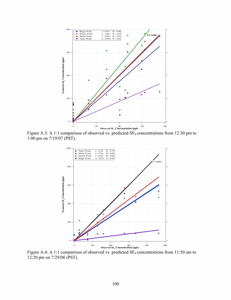
400
300
200
100
0
Pred
icte
d SF
6 Con
cent
ratio
n (p
pt)
4003002001000Observed SF6 Concentration (ppt)
1:1 ratio Briggs 30 min y = 0.87x Pr = 0.90 Draxler 30 min y = 1.20x Pr = 0.93 Martin 30 min y = 0.99x Pr = 0.91 Taylor 30 min y = 0.435x Pr = 0.85
Figure A.3: A 1:1 comparison of observed vs. predicted SF6 concentrations from 12:30 pm to 1:00 pm on 7/19/07 (PST).
1000
800
600
400
200
0
Pred
icte
d SF
6 Con
cent
ratio
n (p
pt)
10008006004002000Observed SF6 Concentration (ppt)
Taylor 30 min y = 0.12x Pr = 0.79 Martin 30 min y = 0.74x Pr = 0.94 Draxler 30 min y = 0.64x Pr = 0.88 Briggs 30 min y = 0.65x Pr = 0.94
1:1 ratio
Figure A.4: A 1:1 comparison of observed vs. predicted SF6 concentrations from 11:50 am to 12:20 pm on 7/29/08 (PST).
100

A.2.2 Statistical Analysis
Various statistical measures were calculated for further analysis of each method. The
statistical measures were: Fractional Bias (FB), Unpaired Peak Prediction Error (UPPE), and
Mean Normalized Gross Error (MNGE). These statistical measures were performed for all
measured SF6 concentrations greater than 50 pptv. The FB, UPPE, and MNGE are defined as:
Fractional Bias (FB) =
[ ][ ]
2),(),(),(),(1
1∑= +
−N
i ioip
ioip
txCtxCtxCtxC
N
Unpaired Peak Prediction Error (UPPE) = mzxo
mzxop
txCtxCtxC
)',()',()',( max −
Mean Normalized Gross Error (MNGE) = %100*),(
),(),(11∑=
−N
i io
ioip
txC
txCtxC
N
where N is the number of concentrations at a given receptor location, and are
the observed and predicted concentrations at the receptor location at x for hour ti, respectively,
and and are the observed and predicted maximum concentrations at a
specific receptor location, respectively. The statistical measures for all sampling periods were
averaged and are given in Table A.6. The lowest value in each category is highlighted in yellow.
),( io txC ),( ip txC
max)',( txCo max)',( txC p
Table A.6: Average Values of Statistical Measures for Various Methods Method FB UPPE MNGEMartin -0.06 0 41 % Briggs -0.11 -0.08 43 % Draxler 0.04 -0.06 60 % Taylor -0.17 -0.7 53 %
Bias statistics measure the tendency of a model to over or under predict observed values.
FB equally weighs positive and negative bias estimates. An FB of zero is ideal. Draxler’s
101

102
method resulted in the lowest average FB values while Taylor’s method yielded the highest.
Martin’s method resulted in the second lowest average FB.
Error is a measure of the extent that the model deviates from the observations. The
UPPE compares the maximum observed and maximum predicted concentrations at a single
sampling period. For the MNGE, a value of zero would indicate that the model exactly matches
the observed values at all points in space/time. Martin’s method resulted in the lowest average
UPPE and MNGE values.
A.2.3 Conclusions
Several methods (Martin, Briggs, Taylor, and Draxler) for determining σy and σz have
been compared with real diffusion data. Through analysis of comparison plots between
predicted and observed SF6 values as well as statistical measures including FB, FGE, and UPPE,
Martin’s method yielded the best results. The average UPPE was zero for Martin’s method,
showing that maximum observed and maximum predicted concentrations closely matched at
every period. The average FB and MNGE for all sampling periods were -0.06 and 41 % for
Martin’s method. Thus, Martin’s method was used for estimating the diffusion coefficients for
SIMFLUX to simulate NH3 and N2O emission rates from potato fields.

A.3 Additional Results
400
300
200
100
0
SF6 C
once
ntra
tion
(ppt
)
14121086420 Receptor Position
Observed Taylor 30 min Briggs 30 min Martin 30 min Draxler 30 min
Figure A.5: Predicted and observed SF6 concentration distribution for Tracer 7/19/07 (Syringe #2, 11:30 am to 12:00 pm PST)
500
400
300
200
100
0
Pred
icte
d SF
6 Con
cent
ratio
n (p
pt)
5004003002001000Observed SF6 Concentration (ppt)
1:1 ratio Martin y = 0.78x Pr = 0.94 Taylor y = 0.36x Pr = 0.83 Draxler y = 0.98x Pr = 0.92 Briggs y = 0.69x Pr = 0.94
Figure A.6: A 1:1 comparison of observed vs. predicted SF6 concentrations for Tracer 7/19/07 (Syringe #2, 11:30 am to 12:00 pm PST)
103

400
300
200
100
0
SF6 C
once
ntra
tion
(ppt
)
1412108642 Receptor Position
Briggs 30 min Draxler 30 min Martin 30 min Observed Taylor 30 min
Figure A.7: Predicted and observed SF6 concentration distribution for Tracer 7/19/07 (Syringe #5, 1:00 pm to 1:30 pm PST)
500
400
300
200
100
0
Pred
icte
d SF
6 Con
cent
ratio
n (p
pt)
5004003002001000Observed SF6 Concentration (ppt)
Briggs 30 min y = 1.08x Pr = 0.92 Draxler 30 min y = 1.42x Pr = 0.93 Martin 30 min y = 1.23x Pr = 0.93 Taylor 30 min y = 0.51x Pr = 0.84
1:1 ratio
Figure A.8: A 1:1 comparison of observed vs. predicted SF6 concentrations for Tracer 7/19/07 (Syringe #5, 1:00 pm to 1:30 pm PST)
104

400
300
200
100
0
SF6
Con
cent
ratio
n (p
pt)
14121086420 Receptor Position
Observed Taylor 30 min Martin 30 min Draxler 30 min Briggs 30 min
Figure A.9: Predicted and observed SF6 concentration distribution for Tracer 7/19/07 (Syringe #6, 1:30 pm to 2:00 pm PST)
500
400
300
200
100
0
Pred
icte
d SF
6 Con
cent
ratio
n (p
pt)
5004003002001000Observed SF6 Concentration (ppt)
Taylor y = 0.47x Pr = 0.83 Martin y = 1.20x Pr = 0.95 Draxler y = 1.47x Pr = 0.96 Briggs y = 1.06x Pr = 0.94
1:1 ratio
Figure A.10: A 1:1 comparison of observed vs. predicted SF6 concentrations for Tracer 7/19/07 (Syringe #6, 1:30 pm to 2:00 pm PST)
105

500
400
300
200
100
0
SF6
Con
cent
ratio
n (p
pt)
14121086420 Receptor Position
Observed Taylor 30 min Martin 30 min Draxler 30 min Briggs 30 min
Figure A.11: Predicted and observed SF6 concentration distribution for Tracer 7/19/07 (Syringe #8, 2:30 pm to 3:00 pm PST)
600
500
400
300
200
100
0
Pred
icte
d SF
6 Con
cent
ratio
n (p
pt)
6005004003002001000Observed SF6 Concentration (ppt)
1:1 ratio
Briggs y = 1.29x Pr = 0.87 Draxler y = 1.76x Pr = 0.89 Martin y = 1.48x Pr = 0.87 Taylor y = 0.60x Pr = 0.81
Figure A.12: A 1:1 comparison of observed vs. predicted SF6 concentrations for Tracer 7/19/07 (Syringe #8, 2:30 pm to 3:00 pm PST)
106

600
500
400
300
200
100
0
SF6
Con
cent
ratio
n (p
pt)
87654321 Receptor Position
Observed Martin 30 min Draxler 30 min Briggs 30 min Taylor 30 min
Figure A.13: Predicted and observed SF6 concentration distribution for Tracer 7/29/08 (Syringe #4, 9:20 am to 9:50 am PST)
600
500
400
300
200
100
0
Pred
icte
d SF
6 Con
cent
ratio
n (p
pt)
6005004003002001000Observed SF6 Concentration (ppt)
Briggs 30 min y = 0.71x Pr = 0.975 Draxler 30 min y = 0.64x Pr = 0.91 Martin 30 min y = 0.82x Pr = 0.974 Taylor 30 min y = 0.19x Pr = 0.75 1:1 ratio
Figure A.14: A 1:1 comparison of observed vs. predicted SF6 concentrations for Tracer 7/29/08 (Syringe #4, 9:20 am to 9:50 am PST)
107

600
400
200
0
SF6
Con
cent
ratio
n (p
pt)
87654321 Receptor Position
Observed Taylor 30 min Martin 30 min Draxler 30 min Briggs 30 min
Figure A.15: Predicted and observed SF6 concentration distribution for Tracer 7/29/08 (Syringe #8, 11:20 am to 11:50 am PST)
800
600
400
200
0
Pred
icte
d SF
6 Con
cent
ratio
n (p
pt)
8006004002000Observed SF6 Concentration (ppt)
Briggs 30 min y = 0.52x Pr = 0.82 Draxler 30 min y = 0.58x Pr = 0.89 Martin 30 min y = 0.61x Pr = 0.83 Taylor 30 min y = 0.165x Pr = 0.90
1:1 ratio
Figure A.16: A 1:1 comparison of observed vs. predicted SF6 concentrations for Tracer 7/29/08 (Syringe #8, 11:20 am to 11:50 am PST)
108

Table A.7: Values of Statistical Measures for Various Sigma Methods for Tracer 7/19/07 (Syringe #2, 11:30 am to 12:00 pm PST)
Method FB MNB MAE MNGE UPPE Martin -0.12 -25% 74.24 45% -0.22 Briggs -0.17 -40% 85.44 48% -0.28 Draxler 0.02 25% 70.70 54% -0.12 Taylor -0.12 -32% 130.88 46% -0.72
Table A.8: Values of Statistical Measures for Various Sigma Methods for Tracer 7/19/07
(Syringe #5, 1:00 pm to 1:30 pm PST) Method FB MNB MAE MNGE UPPE Martin 0.02 18% 79.25 44% 0.15 Briggs -0.04 -1% 63.44 38% 0.06
Draxler 0.11 59% 100.59 59% 0.09 Taylor -0.12 -38% 85.71 38% -0.66
Table A.9: Values of Statistical Measures for Various Sigma Methods for Tracer 7/19/07
(Syringe #6, 1:30 pm to 2:00 pm PST) Method FB MNB MAE MNGE UPPE Martin 0.03 16% 58.05 23% 0.28 Briggs -0.03 -5% 65.36 32% 0.17 Draxler 0.13 78% 128.32 78% 0.36 Taylor -0.10 -25% 115.45 50% -0.59
Table A.10: Values of Statistical Measures for Various Sigma Methods for Tracer 7/19/07
(Syringe #8, 2:30 pm to 3:00 pm PST) Method FB MNB MAE MNGE UPPE Martin -0.05 14% 115.18 70% 0.58 Briggs -0.10 -7% 101.55 66% 0.45 Draxler 0.14 90% 137.90 93% 0.40 Taylor -0.07 -22% 55.70 27% -0.33
Table A.11: Values of Statistical Measures for Various Sigma Methods for Tracer 7/29/08
(Syringe #4, 9:20 am to 9:50 am PST) Method FB MNB MAE MNGE UPPE Martin -0.05 -15% 69.36 23% -0.24 Briggs -0.09 -29% 98.61 29% -0.24
Draxler -0.05 -13% 118.44 31% -0.51 Taylor -0.28 -71% 264.82 71% -0.87
109

Table A.12: Values of Statistical Measures for Various Sigma Methods for Tracer 7/29/08 (Syringe #8, 11:20 am to 11:50 am PST)
Method FB MNB MAE MNGE UPPE Martin -0.18 -48% 178.40 48% -0.26 Briggs -0.22 -57% 214.62 57% -0.33
Draxler -0.11 -28% 184.98 50% -0.27 Taylor -0.25 -57% 350.85 68% -0.84
110

APPENDIX B: ADDITIONAL N2O RESULTS
111
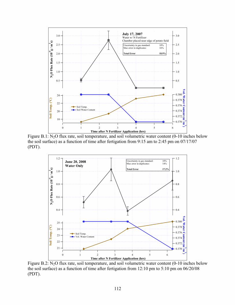
3.0 3.0
2.5 2.5
2.0 2.0
1.5 1.5
1.0 1.0
0.5 0.5
N2O
Flu
x R
ate
(10-4
g / m
2 s)
6543210 Time after N Fertilizer Application (hrs)
24
22
20
18
July 17, 2007Water w/ N FertilizerChamber placed near edge of potato fieldUncertainty in gas standard: 10%Max error in duplicates: 16% Total Error 18.9%
0.380
Soi
l Tem
p. (º
C)
0.378
0.376
0.374
0.372
0.370
Vol. W
ater Content (m
3/m3)
Soil Temp. Soil Water Content
Figure B.1: N2O flux rate, soil temperature, and soil volumetric water content (0-10 inches below the soil surface) as a function of time after fertigation from 9:15 am to 2:45 pm on 07/17/07 (PDT).
1.2 1.2
1.0 1.0
0.8 0.8
0.6 0.6
0.4 0.4
N2O
Flu
x R
ate
(10-4
g / m
2 s)
6543210 Time after N Fertilizer Application (hrs)
25
24
23
22
21
Soi
l Tem
p. (º
C)
0.380
0.378
0.376
0.374
0.372
June 20, 2008Water Only
Uncertainty in gas standard: 10%Max error in duplicates: 14% Total Error 17.2%
0.370
Vol. W
ater Content (m
3/m3)
Soil Temp. Vol. Water Content
Figure B.2: N2O flux rate, soil temperature, and soil volumetric water content (0-10 inches below the soil surface) as a function of time after fertigation from 12:10 pm to 5:10 pm on 06/20/08 (PDT).
112

1.6 1.6
1.4 1.4
1.2 1.2
1.0 1.0
0.8 0.8
0.6 0.6
0.4 0.4
0.2 0.2
0.0 0.0
N2O
Flu
x R
ate
(10-4
g / m
2 s)
6543210 Time after N Fertilizer Application (hrs)
20
18
16
14
Soi
l Tem
p. (º
C)
0.46
0.44
0.42
0.40
June 21, 2008Water Only
Uncertainty in gas standard: 10%Max error in duplicates: 5% Total Error 11.2% chamber 11
chamber 12 chamber 13 average
Vol. W
ater Content (m
3/m3)
Soil Temp. Vol. Water Content
Figure B.3: N2O flux rate, soil temperature, and soil volumetric water content (0-10 inches below the soil surface) as a function of time after fertigation from 9:45 pm to 3:15 pm on 06/21/08 (PDT).
1.2 1.2
1.0 1.0
0.8 0.8
0.6 0.6
0.4 0.4
N2O
Flu
x R
ate
(10-4
g / m
2 s)
543210 Time after N Fertilizer Application (hrs)
18.5
18.0
17.5
17.0
16.5
16.0
Soi
l Tem
p. (º
C)
0.460
0.458
0.456
0.454
0.452
July 22, 2008Water w/ N FertilizerUncertainty in gas standard: 10%Max error in duplicates: 18% Total Error 20.6%
0.450
Vol. W
ater Content (m
3/m3)
Soil Temp. Vol. Water Content
Figure B.4: N2O flux rate, soil temperature, and soil volumetric water content (0-10 inches below the soil surface) as a function of time after fertigation from 9:45 am to 2:30 pm on 07/22/08 (PDT).
113

114
APPENDIX C:
ADDITIONAL NH3 RESULTS

C.1 Application Rates Calculations: N application rate (12 deg hr-1 sprinkler arm rotation rate):
s2m
gN47.8E
400m*10m
1*
1lb
453.6g*
60s
1min*
30min
6deg*
360deg
1rotation*124.2acres*
rotation*acre
lbsN6 −=
N application rate (18 deg hr-1 sprinkler arm rotation rate):
s2m
gN411.7E
400m*10m
1*
1lb
453.6g*
60s
1min*
30min
9deg*
360deg
1rotation*124.2acres*
rotation*acre
lbsN6 −=
NH3 application rate by sprinkler arm (400 m by 10 m) (12 deg hr-1 sprinkler arm rotation rate):
s2m3
gNH49.5E
/143/17
*400m*10m
1*
1lb
453.6g*
60s
1min*
30min
6deg*
360deg
1rotation*124.2acres*
rotation*acre
lbsN6 −=
molNg
molNHg
NH3 application rate by sprinkler arm (400 m by 10 m) (18 deg hr-1 sprinkler arm rotation rate):
s2m3
gNH414.25E
/143/17
*400m*10m
1*
1lb
453.6g*
60s
1min*
30min
9deg*
360deg
1rotation*124.2acres*
rotation*acre
lbsN6 −=
molNg
molNHg
115

C.2 Additional NH3 Concentrations Results
20 20
15 15
10 10
5 5
0 0
NH
3 Con
c. (p
pbv)
6:00 PM7/8/2007
6:00 PM7/8/2007
9:00 PM
9:00 PM
12:00 AM7/9/2007
12:00 AM7/9/2007
3:00 AM
3:00 AM
6:00 AM
6:00 AM
9:00 AM
9:00 AM
12:00 PM
12:00 PM
3:00 PM
3:00 PM
6:00 PM
6:00 PM
Date/Time (PDT)
2.4
2.2
2.0
1.8
1.6
WS
(m/s
)
350
300
250
200
150
WD
(deg)
30 30
28 28
26 26 Tem
p. (º
C)
Fertigation Error: ± 3ppbv ± 30%
detection limit
ws wd
air soil surface
Figure C.1: Time series plot of measured 30-minute average NH3 concentration, wind speed, wind direction, air temperature, and soil surface temperature from 5 pm on 07/08/07 to 6 pm on 07/09/07.
Figure C.2: Polar plot of NH3 concentration versus sprinkler arm rotation angle (red circles) and wind direction (blue squares) for 4:30 pm to 6 pm 07/09/07 (PDT).
116

30 30
20 20
10 10
0 0
NH
3 Con
c. (p
pbv)
12:00 PM7/11/2007
12:00 PM7/11/2007
4:00 PM
4:00 PM
8:00 PM
8:00 PM
12:00 AM7/12/2007
12:00 AM7/12/2007
4:00 AM
4:00 AM
8:00 AM
8:00 AM
12:00 PM
12:00 PM
Date/Time (PDT)
54321
WS
(m/s
)
360
320
280
240
WD
(deg)
35 35
30 30
25 25
Tem
p. (º
C)
Fertigation
Error: ± 3ppbv ± 30%
detection limit
ws wd
air soil surface
Figure C.3: Time series plot of measured 30-minute average NH3 concentration, wind speed, wind direction, air temperature, and soil surface temperature from 11 am on 07/11/07 to 3 pm 07/12/07.
Figure C.4: Polar plot of NH3 concentration versus sprinkler arm rotation angle (red circles) and wind direction (blue squares) for 11 am to 7:30 pm 07/11/07 (PDT).
117

Figure C.5: Polar plot of NH3 concentration versus sprinkler arm rotation angle (red circles) and wind direction (blue squares) for 9 am to 3 pm on 07/12/07 (PDT).
50 50
40 40
30 30
20 20
10 10
0 0
NH
3 Con
c. (p
pbv)
12:00 PM7/18/2007
12:00 PM7/18/2007
4:00 PM
4:00 PM
8:00 PM
8:00 PM
12:00 AM7/19/2007
12:00 AM7/19/2007
4:00 AM
4:00 AM
8:00 AM
8:00 AM
12:00 PM
12:00 PM
4:00 PM
4:00 PM
Date/Time (PDT)
4.0
3.0
2.0 WS
(m/s
)
280
240
200
WD
(deg)
28 2826 2624 2422 2220 20
Tem
p. (º
C)
No Irrigation or Fertigation
Fertigation
Error: ± 3 ppbv ± 30%
detection limit
ws wd
air soil surface
Figure C.6: Time series plot of measured 30-minute average NH3 concentration, wind speed, wind direction, air temperature, and soil surface temperature from 12 pm on 07/18/07 to 4 pm on 07/19/07.
118

Figure C.7: Polar plot of NH3 concentration versus sprinkler arm rotation angle (red circles) and wind direction (blue squares) for 12 pm to 5:30 pm on 07/18/07 (PDT).
Figure C.8: Polar plot of NH3 concentration versus sprinkler arm rotation angle (red circles) and wind direction (blue squares) for 12 pm to 4 pm on 07/19/07 (PDT).
119

120 120
100 100
80 80
60 60
40 40
20 20
0 0
NH
3 Con
c. (p
pbv)
12:00 PM7/23/2008
12:00 PM7/23/2008
3:00 PM
3:00 PM
6:00 PM
6:00 PM
9:00 PM
9:00 PM
12:00 AM7/24/2008
12:00 AM7/24/2008
3:00 AM
3:00 AM
6:00 AM
6:00 AM
9:00 AM
9:00 AM
12:00 PM
12:00 PM
Date and Time (PDT)
4
3
2
1
0
WS
(m/s
) 300
200
100
WD
(deg)
30 30
20 20
10 10 Tem
p. (C
)
No Irrigation or Fertigation
Fertigation
Error = ± 3 ppbv ± 30%
detection limit
ws wd
air soil surface
Figure C.9: Time series plot of measured 30-minute average NH3 concentration, wind speed, wind direction, air temperature, and soil surface temperature from 11 am on 07/23/08 to 1 pm on 07/24/08.
Figure C.10: Polar plot of NH3 concentration versus sprinkler arm rotation angle (red circles) and wind direction (blue squares) for 11 am to 4 pm on 07/23/08 (PDT).
120

Figure C.11: Polar plot of NH3 concentration versus sprinkler arm rotation angle (red circles) and wind direction (blue squares) for 4:30 pm to 11:30 pm on 07/23/08 (PDT).
Figure C.12: Polar plot of NH3 concentration versus sprinkler arm rotation angle (red circles) and wind direction (blue squares) for 11:30 pm on 7/23/08 to 2 am on 07/24/08 (PDT).
121

Figure C.13: Polar plot of NH3 concentration versus sprinkler arm rotation angle (red circles) and wind direction (blue squares) for 2:30 am to 5 am on 07/24/08 (PDT).
Figure C.14: Polar plot of NH3 concentration versus sprinkler arm rotation angle (red circles) and wind direction (blue squares) for 7 am to 1 pm on 07/24/08 (PDT).
122

12 12
8 8
4 4
0 0
NH
3 Con
c. (p
pbv)
12:00 PM7/28/2008
12:00 PM7/28/2008
3:00 PM
3:00 PM
6:00 PM
6:00 PM
9:00 PM
9:00 PM
12:00 AM7/29/2008
12:00 AM7/29/2008
3:00 AM
3:00 AM
6:00 AM
6:00 AM
9:00 AM
9:00 AM
12:00 PM
12:00 PM
3:00 PM
3:00 PM
Date and Time (PDT)
6
4
2
0
WS
(m/s
)
280
240
200
160
WD
(deg)
30 30
20 20
10 10 Tem
p. (°
C)
No Irrigation or Fertigation
Irrigation
Error: ±3 ppbv ± 30%
detection limit
ws wd
air soil surface
Figure C.15: Time series plot of measured 30-minute average NH3 concentration, wind speed, wind direction, air temperature, and soil surface temperature from 10 am on 07/28/08 to 2:30 pm on 07/29/08.
123

C.3 Additional NH3 Flux Rates Results
3.5
3.5
3.0
3.0
2.5
2.5
2.0
2.0
1.5
1.5
1.0
1.0
0.5
0.5
0.0
0.0
WS (m/s)
80 80
60 60
40 40
20 20
0 0
WD
Sig
ma
(deg
)
07/08/07 07/09/07 07/11/07 07/12/07 07/18/07 07/19/07 07/23/08 07/24/08A 07/24/08B 07/26/08 07/27/08 07/28/08 07/29/08
Figure C.16: Wind speed vs. wind direction sigma (given in 30-min averages) for all days of NH3 measurement. Low wind speeds are associated with large variation in wind direction. Periods with large variation in wind direction (greater than 30 deg) and low wind speeds (less than 1 m s-1) should not be included in determining NH3 flux rates since the theoretical basis of the Gaussian plume dispersion model becomes invalid.
10 10
8 8
6 6
4 4
2 2
NH
3/WS
(ppb
v/m
/s)
4.0
4.0
3.5
3.5
3.0
3.0
2.5
2.5
2.0
2.0
1.5
1.5
WS (m/s)
close far
Fertigation Periods
Figure C.17: NH3 concentrations (ppbv) normalized by wind speed (m s-1) as a function of wind speed (m s-1).
124

Figure C.18: NH3 concentrations normalized by wind speed (m s-1) as a function of wind direction (deg) for fertigation periods when the DOAS measurement path was in the SE quadrant of the potato fields
Figure C.19: NH3 concentrations normalized by wind speed (m s-1) as a function of wind direction (deg) for fertigation periods when the DOAS measurement path was in the NE quadrant of the potato fields.
125

Figure C.20: NH3 concentrations normalized by wind speed (m s-1) as a function of wind direction (deg) for periods of no irrigation or fertigation.
10 10
8 8
6 6
4 4
2 2
NH
3/WS
(ppb
v/m
/s)
34
34
33
33
32
32
31
31
30
30
29
29
28
28
27
27
26
26
25
25
24
24
23
23
22
22
21
21
Temperature (°C)
air, close air, far soil surface, close soil surface, far
Fertigation Periods
Figure C.21: NH3 concentrations normalized by wind speed (m s-1) as a function of soil surface and air temperature (°C) for fertigation periods.
126

300 300
250 250
200 200
150 150
100 100
50 50
NH
3 Fl
ux R
ate
(µg
m-2
s-1)
34
34
32
32
30
30
28
28
26
26
24
24
22
22
Temperature (°C)
Fertigation Periods
Air Temperature: far close Soil Temperature: far close
Figure C.22: NH3 flux rates (μg m-2s-1) as a function of soil surface and air temperature (°C) for fertigation periods.
7 7
6 6
5 5
4 4
3 3
NH
3/WS
(ppb
v/m
/s)
25
25
20
20
15
15
Temperature (°C)
soil surface air
Periods of No Irrigation or Fertigation
Figure C.23: NH3 concentrations normalized by wind speed (m s-1) as a function of soil surface and air temperature (°C) for periods of no irrigation or fertigation.
127

2.2 2.2
2.0 2.0
1.8 1.8
1.6 1.6
1.4 1.4
1.2 1.2
1.0 1.0
0.8 0.8
0.6 0.6
NH
3 Fl
ux R
ate
(µg
m-2
s-1)
28
28
26
26
24
24
22
22
20
20
18
18
16
16
14
14
12
12
Temperature (°C)
Air Soil Surface
Periods of No Irrigation or Fertigation
Figure C.24: NH3 flux rates (μg m-2s-1) as a function of soil surface and air temperature (°C) for periods of no irrigation or fertigation.
300 300
250 250
200 200
150 150
100 100
50 50
NH
3 Fl
ux R
ate
(µg
m-2
s-1)
11:00 AM1/1/1904
11:00 AM1/1/1904
12:00 PM
12:00 PM
1:00 PM
1:00 PM
2:00 PM
2:00 PM
3:00 PM
3:00 PM
4:00 PM
4:00 PM
5:00 PM
5:00 PM
Time of Day (PDT)
close far
Fertigation Periods
Figure C.25: NH3 flux rates (μg m-2 s-1) as a function of time of day for fertigation periods.
128

2.0 2.0
1.8 1.8
1.6 1.6
1.4 1.4
1.2 1.2
1.0 1.0
0.8 0.8
0.6 0.6
NH
3 Fl
ux R
ate
(µg
m-2
s-1)
10:00 AM1/1/1904
10:00 AM1/1/1904
12:00 PM
12:00 PM
2:00 PM
2:00 PM
4:00 PM
4:00 PM
Time of Day (PDT)
Periods of No Irrigation or Fertigation
day after irrigation day after fertigation
Figure C.26: Temperature (°C) as a function of time of day (PDT) for periods of no irrigation or fertigation
300 300
250 250
200 200
150 150
100 100
50 50
NH
3 Flu
x R
ate
(µg
m-2
s-1)
180
180
160
160
140
140
120
120
100
100
80
80
60
60
40
40
20
20
Angle between Sprinkler Arm and Wind Direction (deg)
close far
Fertigation Periods
Figure C.27: Adjusted and non-adjusted NH3 flux rates (μg m-2 s-1) as a function of the angle between the sprinkler arm and wind direction (deg).
129

180 180
160 160
140 140
120 120
100 100
80 80
60 60
40 40
20 20
Ang
le b
etw
een
Spri
nkle
r A
rm a
nd W
D (d
eg)
4.4
4.4
4.2
4.2
4.0
4.0
3.8
3.8
3.6
3.6
3.4
3.4
3.2
3.2
3.0
3.0
2.8
2.8
2.6
2.6
2.4
2.4
2.2
2.2
2.0
2.0
1.8
1.8
1.6
1.6
WS (m/s)
Fertigation Periods
close far
Figure C.28: Angle between sprinkler arm and wind direction (deg) as a function of wind speed (m s-1).
130