measurement · pdf filewhy study measurement systems? • in design stage, ... functional...

Measurement SystemsLecture 1- General Concepts

Hamid AhmadianSchool of Mechanical EngineeringIran University of Science and [email protected]

Types of Applications ofMeasurement Instrumentation

• WHY STUDY MEASUREMENT SYSTEMS?

• CLASSIFICATION OF TYPES OF MEASUREMENT APPLICATIONS

• COMPUTER-AIDED MACHINES AND PROCESSES

WHY STUDY MEASUREMENT SYSTEMS?

“Measurement system” includes all components in a chain of hardware and software that leads from the measured variable to processed data.

Let’s introduce some basic ideas using the automotive industry as an example.

Modern automobile uses as many as 40 or 50 sensors (measuring devices) in implementing various functions.


• In design stage, one must be aware of the instruments available▫ for the various measurements, and ▫ how they operate and interface with other parts of the

system. ▫ keep up with new sensor developments to allow

improvements in car design and operation. • Lack of such sensor knowledge can severely restrict

the range of designs that one can conceive, thus limiting improvements in overall car performance.


• Laboratory testing and the associated measurement systems are a vital part of the design process:▫ If a new material is being considered, we may need to

run strength tests to develop data needed by the design engineers.

▫ Or, a new or revised manufacturing process may require statistical response surface experiments to find the effects of process variables on performance and/or cost.

▫ Finally, availability from suppliers of new components, such as improved shock absorbers, may require performance testing to decide whether their use is warranted in the new design.


• As design and development proceed, prototype subsystems and finally entire vehicles will be produced.

• These are used as "test beds" to evaluate performance and then feed back information to the design/manufacturing teams.

• Once the design has been finalized, then manufacture of the product in quantity can commence,▫ the manufacturing tools are controlled by a so-called

feedback mechanism▫ some quality parameter of the part produced is

measured with appropriate sensors.


• The final product, a modern automobile, relies on a multitude of sensors for its optimum operation:▫ Speedometers tell us the vehicle's speed▫ Tachometers display engine RPM▫ Fuel gages keep track of the gas supply▫ Temperature sensors warn of overheating▫ GPS to locate the car and guide the driver▫ Accelerometers signal air bags to deploy in case of a crash ▫ Brake-cylinder pressure and wheel-speed sensors control

the antilock braking system▫ GyroChip to measure angular velocity to augment vehicle

stability during severe or emergency maneuvers.

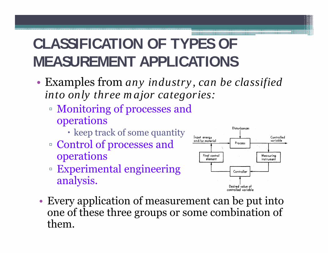
CLASSIFICATION OF TYPES OFMEASUREMENT APPLICATIONS• Examples from any industry, can be classified

into only three major categories:▫ Monitoring of processes and

operations keep track of some quantity

▫ Control of processes and operations

▫ Experimental engineering analysis.

• Every application of measurement can be put into one of these three groups or some combination of them.

General Concepts:• Chapter 2: Generalized Configurations and

Functional Descriptions of Measuring Instruments ▫ Functional Elements of an Instrument▫ Active and Passive Transducers▫ Analog and Digital Modes of Operation▫ Null and Deflection Methods▫ Input-Output Configuration of Instruments and

Measurement Systems▫ Methods of Correction for Interfering and Modifying Inputs

• Chapter 3: Generalized Performance Characteristics of Instruments▫ Static Characteristics and Static Calibration▫ Dynamic Characteristics

Measuring Devices• Chapter4: Motion and Dimensional Measurement• Chapter 5: Force, Torque, and Shaft Power

Measurement• Chapter 6: Pressure and Sound Measurement• Chapter 7: Flow Measurement• Chapter 8: Temperature and Heat-Flux

Measurement

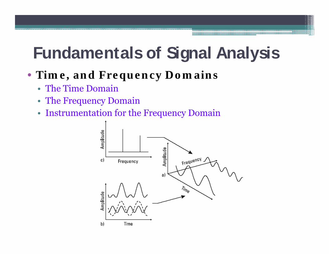
Fundamentals of Signal Analysis• Time, and Frequency Domains

• The Time Domain• The Frequency Domain • Instrumentation for the Frequency Domain

Fundamentals of Signal AnalysisUnderstanding Dynamic Signal Analysis FFT Properties Sampling and Digitizing Aliasing Band Selectable Analysis Windowing Averaging Real Time Bandwidth Overlap Processing

Using Dynamic Signal Analyzers

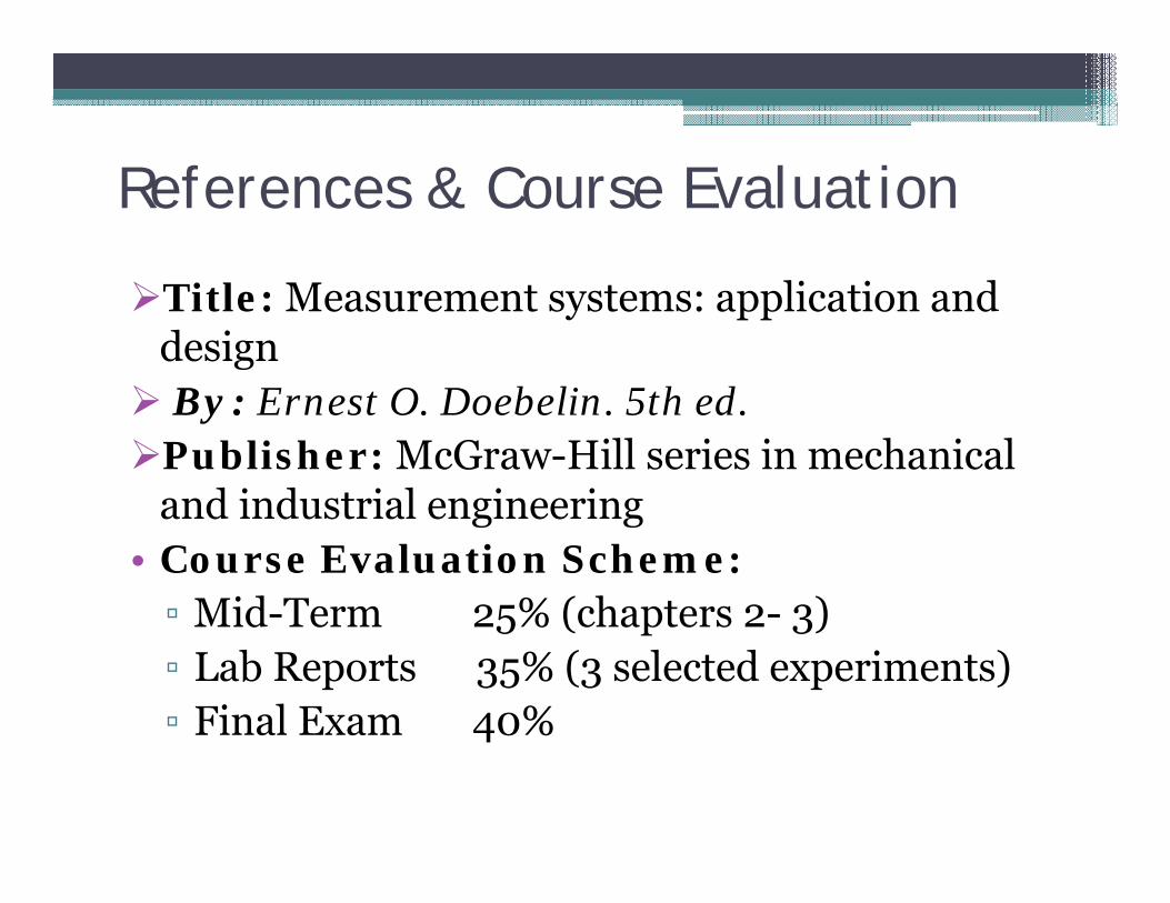
References & Course Evaluation

Title: Measurement systems: application and design By: Ernest O. Doebelin. 5th ed.Publisher: McGraw-Hill series in mechanical

and industrial engineering• Course Evaluation Scheme:▫ Mid-Term 25% (chapters 2- 3)▫ Lab Reports 35% (3 selected experiments)▫ Final Exam 40%

Measurement SystemsLecture 2- Generalized Configurations and Functional Descriptions of Measuring Instruments


Generalized Configurations and Functional Descriptions of Measuring Instruments

• Functional Elements of an Instrument• Active and Passive Transducers• Analog and Digital Modes of Operation• Null and Deflection Methods• Input-Output Configuration of Instruments

and Measurement Systems▫ Methods of Correction for Interfering and

Modifying Inputs

Functional Elements of an Instrument

• In general without recourse to specific physical hardware, one may describe both the operation and the performance of measuring instruments,▫ The operation can be described in terms of the

functional elements of instrument systems, such scheme helps to understand the operation of

any new instrument with which one may come in contact and to plan the design of a new instrument.

▫ The performance is defined in terms of the static and dynamic performance characteristics.

4

Functional Elements of an Instrument

Simple Instrument Model

Mass of an object

Weight

(Observable Physical Variable)

Key functional

element

Mechanical or Electrical

(Can be Manipulated in a Transmission System)

The Measurement

(Observed Output)

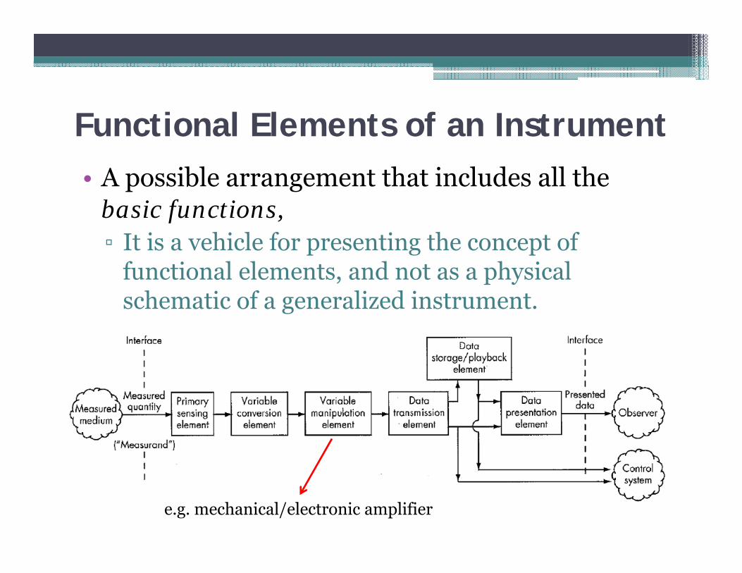
Functional Elements of an Instrument• A possible arrangement that includes all the

basic functions,▫ It is a vehicle for presenting the concept of

functional elements, and not as a physical schematic of a generalized instrument.

e.g. mechanical/electronic amplifier

Functional Elements of an InstrumentPressure gage

• The primary sensing element is the piston, which also serves the function of variable conversion element

Functional Elements of an InstrumentPressure thermometer

• The liquid-filled bulb acts as a primary sensor and variable-conversion element▫ a temperature

change results in a pressure buildup within the bulb

Active and Passive Transducers• One may group the instruments based on energy

considerations:▫ a physical component may act as an active

transducer or a passive transducer.• Passive transducer :A component whose output

energy is supplied entirely by its input signal• An active transducer has an auxiliary source of

power which supplies a major part of the output power while the input signal supplies only an insignificant portion.

9

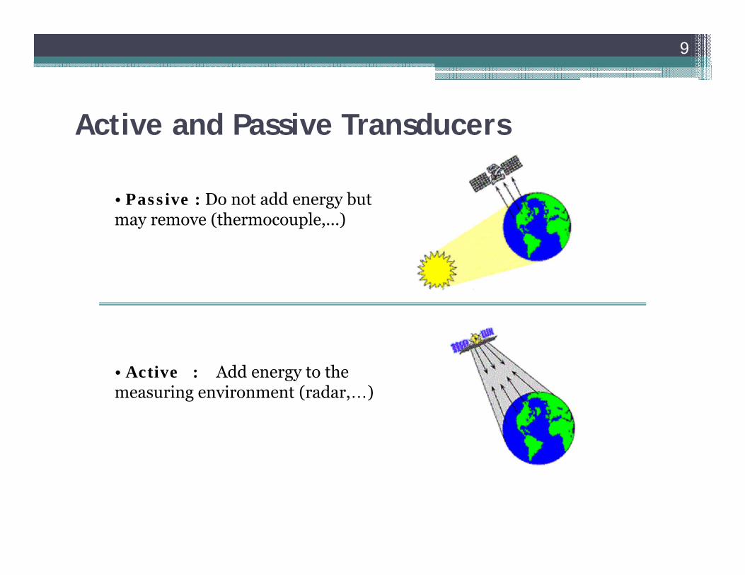
Active and Passive Transducers

• Passive : Do not add energy but may remove (thermocouple,...)

• Active : Add energy to the measuring environment (radar,…)

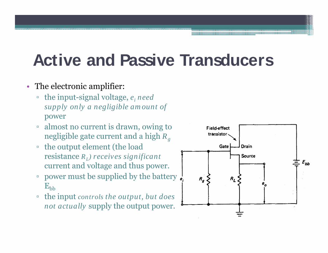
Active and Passive Transducers• The electronic amplifier:▫ the input-signal voltage, ei need

supply only a negligible amount of power

▫ almost no current is drawn, owing to negligible gate current and a high Rg

▫ the output element (the load resistance RL) receives significant current and voltage and thus power.

▫ power must be supplied by the battery Ebb

▫ the input controls the output, but does not actually supply the output power.

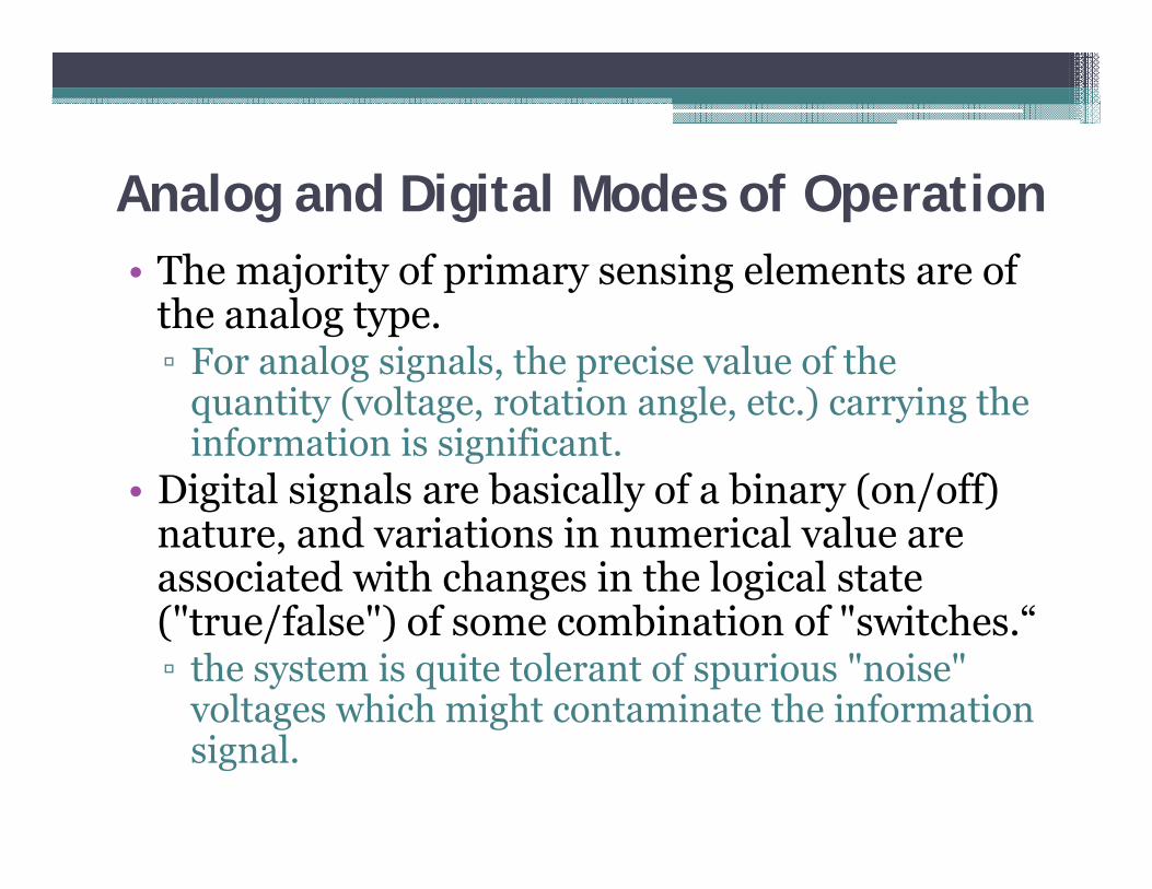
Analog and Digital Modes of Operation• The majority of primary sensing elements are of

the analog type.▫ For analog signals, the precise value of the

quantity (voltage, rotation angle, etc.) carrying the information is significant.

• Digital signals are basically of a binary (on/off) nature, and variations in numerical value are associated with changes in the logical state ("true/false") of some combination of "switches.“▫ the system is quite tolerant of spurious "noise"

voltages which might contaminate the information signal.

12

Null and Deflection Methods

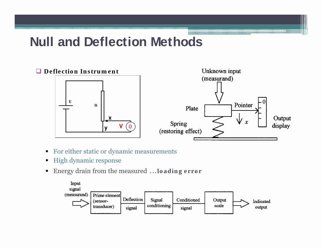
Deflection Instrument

For either static or dynamic measurements High dynamic response

Energy drain from the measured …loading error

13

Null and Deflection Methods

Null Instrument

- Key features- Comparator for Iterative balancing operation- Feedback to achieve balance- Null deflection at parity

High accuracy for small input values Low loading error Not suitable for high speed measurements

Measurement SystemsLecture 3- Input-Output Configuration of Instruments and Measurement Systems


INPUT-OUTPUT CONFIGURATION OFINSTRUMENTS AND MEASUREMENT SYSTEMS• A generalized configuration

containing the significant input -output relationships present in all measuring apparatus,▫ A scheme suggested by

Draper, McKay, and Lees• Desired inputs : quantities

that the instrument is specifically intended to measure.

• Interfering inputs :quantities to which the instrument is unintentionally sensitive.

• Modifying inputs are the quantities that cause a change in the input-output relations for the desired and interfering inputs

Examples: Interfering/Modifying inputs

The desired inputs p1and p2 whose difference causes the output x, which can be read off the calibrated scale

Measuring pressures under acceleration influence; an error will be engenderedbecause of the interfering acceleration input.

If the manometer is not properly aligned with the gravity vector, it give an interfering output signal (also a modifying input).

Modifying inputs: ambient temperature and gravitational force.

Both the desired and the interfering inputs may be altered by the modifying inputs.

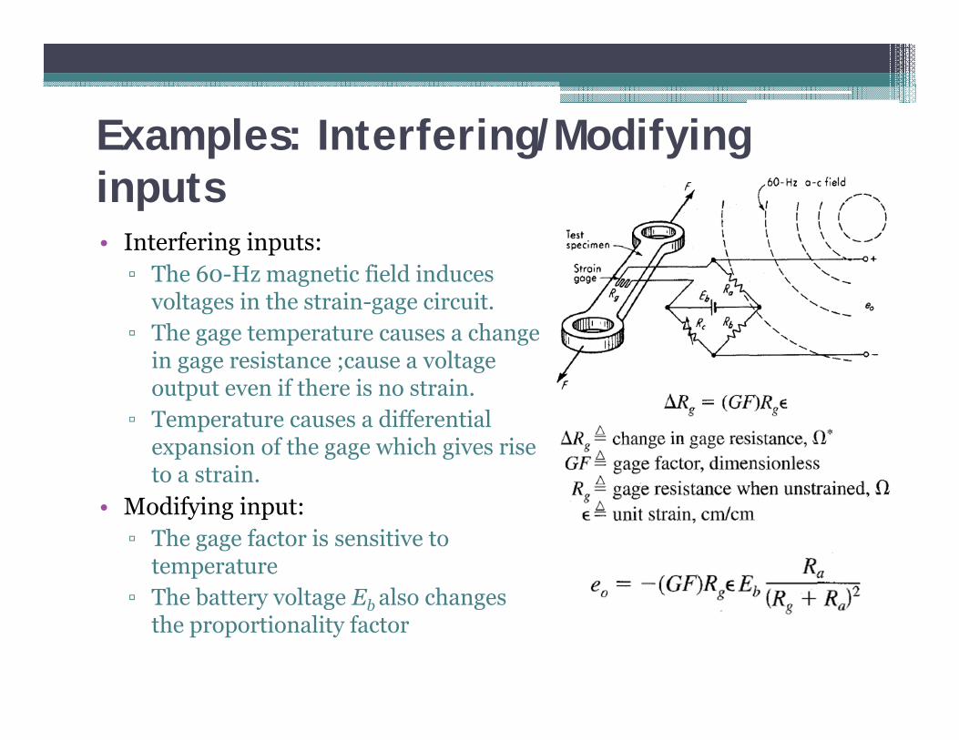
Examples: Interfering/Modifying inputs • Interfering inputs:▫ The 60-Hz magnetic field induces

voltages in the strain-gage circuit.▫ The gage temperature causes a change

in gage resistance ;cause a voltage output even if there is no strain.

▫ Temperature causes a differential expansion of the gage which gives rise to a strain.

• Modifying input:▫ The gage factor is sensitive to

temperature▫ The battery voltage Eb also changes

the proportionality factor

Methods of Correction for Interfering and Modifying Inputs

• A number of methods for nullifying/reducing the effects of spurious inputs are available:▫ The method of inherent insensitivity▫ The method of high-gain feedback▫ The method of calculated output corrections▫ The method of signal filtering▫ The method of opposing inputs

The method of inherent insensitivity

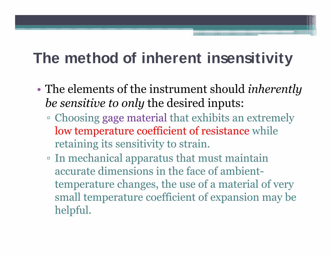
• The elements of the instrument should inherently be sensitive to only the desired inputs:▫ Choosing gage material that exhibits an extremely

low temperature coefficient of resistance while retaining its sensitivity to strain.

▫ In mechanical apparatus that must maintain accurate dimensions in the face of ambient-temperature changes, the use of a material of very small temperature coefficient of expansion may be helpful.

The method of high-gain feedback

• E.g.: Measuring a voltage ei by applying it to a motor whose torque acts on a spring, causing a displacement x0

Open-loop system

The method of high-gain feedback

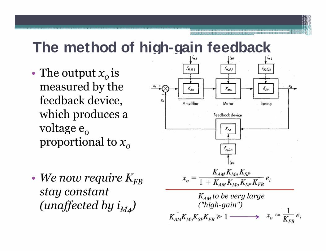
• The output x0 is measured by the feedback device, which produces a voltage e0proportional to x0

• We now require KFBstay constant (unaffected by iM4)

KAM to be very large ("high-gain")

The method of calculated output corrections• Requires to measure or estimate the magnitudes

of the interfering and/or modifying inputs and to know quantitatively how they affect the output:▫ In the manometer the effects of temperature on

both the calibrated scale's length and the density of mercury may be quite accurately computed.

▫ The local gravitational acceleration is known for a given elevation and latitude, so that this effect may be corrected.

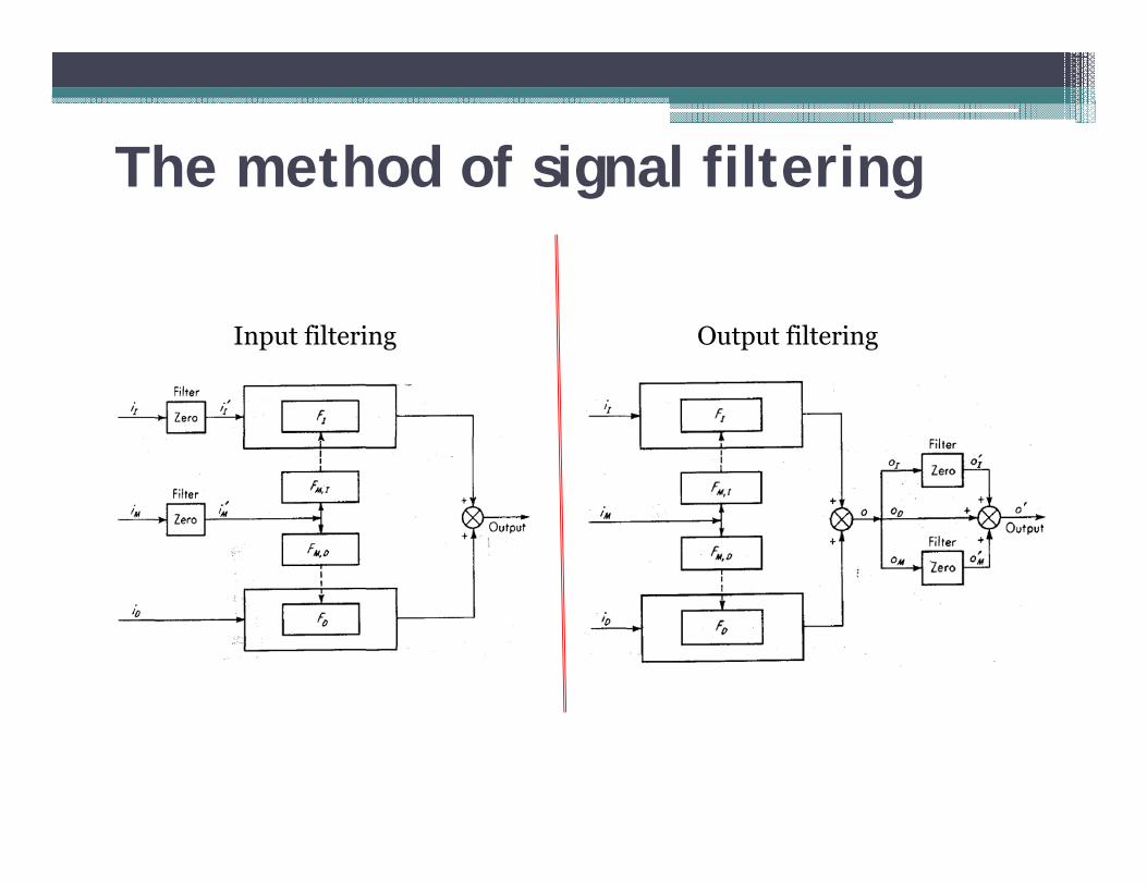
The method of signal filtering

Input filtering Output filtering

The method of input signal filtering

• Electromechanical devices for navigation and control of aircraft or missiles,▫ The interfering vibration

input may be filtered out by use of suitable spring mounts.

• The interfering tilt-angle input to the manometer may be effectively filtered out by means of the gimbal-mounting

The method of input signal filtering

• The thermocouple reference junction is shielded from ambient temperature fluctuations.

• Such an arrangement acts as a filter for temperature or heat-flow inputs

• The strain-gage circuit is shielded from the interfering 60-Hz field

The method of output signal filtering• The strains to be measured are mainly steady and never

vary more rapidly than 2 Hz. • It is possible to insert a simple RC filter that will pass

the desired signals but almost completely block the 60-Hz interference.

The method of output signal filtering

• The pressure gage modified by the insertion of a flow restriction between the source of pressure and the piston chamber,▫ The pulsations in the air pressure may be

smoothed by the pneumatic filtering effect of the flow restriction and associated volume.

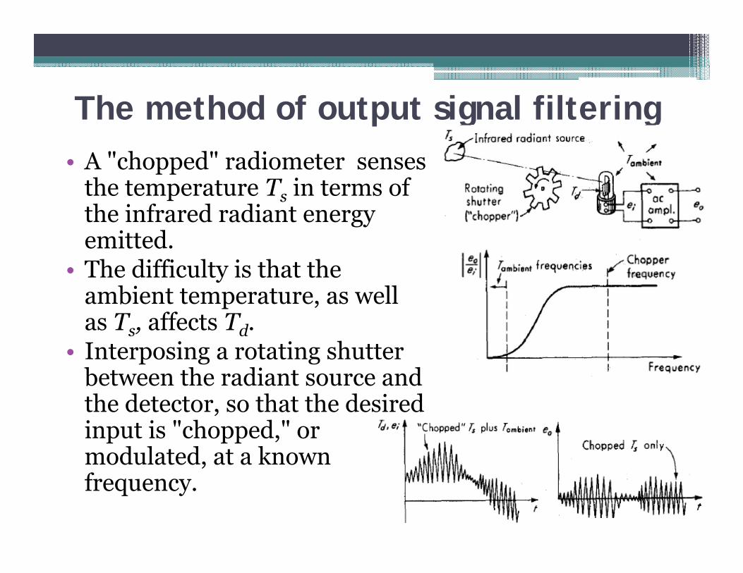
The method of output signal filtering• A "chopped" radiometer senses

the temperature Ts in terms of the infrared radiant energy emitted.

• The difficulty is that the ambient temperature, as well as Ts, affects Td.

• Interposing a rotating shutter between the radiant source and the detector, so that the desired input is "chopped," or modulated, at a known frequency.

The method of opposing inputs• Intentionally introducing into the instrument

interfering and/or modifying inputs that tend to cancel the bad effects of the unavoidable spurious inputs.

The method of opposing inputs

• A millivoltmeter is basically a current-sensitive device.

• However, as long as the total circuit resistance is constant, its scale can be calibrated in voltage, since voltage and current are proportional.

The method of opposing inputs

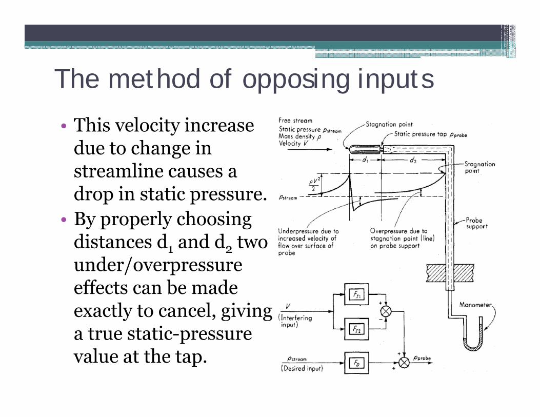
• This velocity increase due to change in streamline causes a drop in static pressure.

• By properly choosing distances d1 and d2 two under/overpressure effects can be made exactly to cancel, giving a true static-pressure value at the tap.

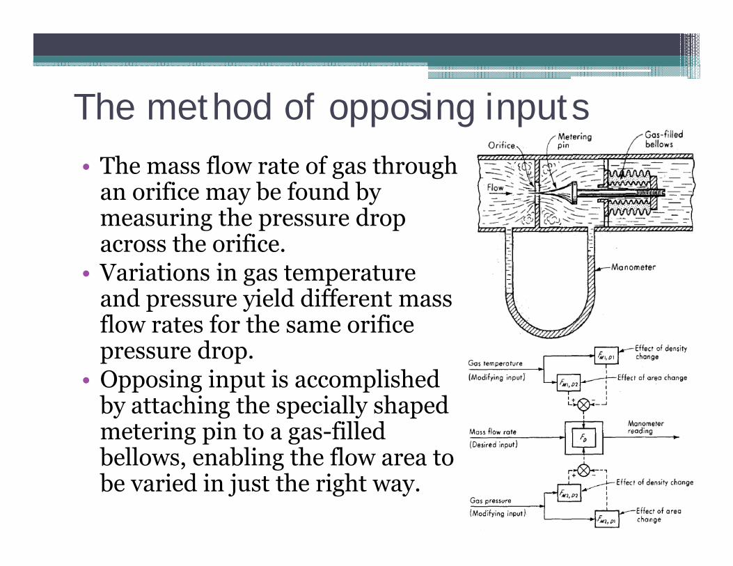
The method of opposing inputs• The mass flow rate of gas through

an orifice may be found by measuring the pressure drop across the orifice.

• Variations in gas temperature and pressure yield different mass flow rates for the same orifice pressure drop.

• Opposing input is accomplished by attaching the specially shaped metering pin to a gas-filled bellows, enabling the flow area to be varied in just the right way.

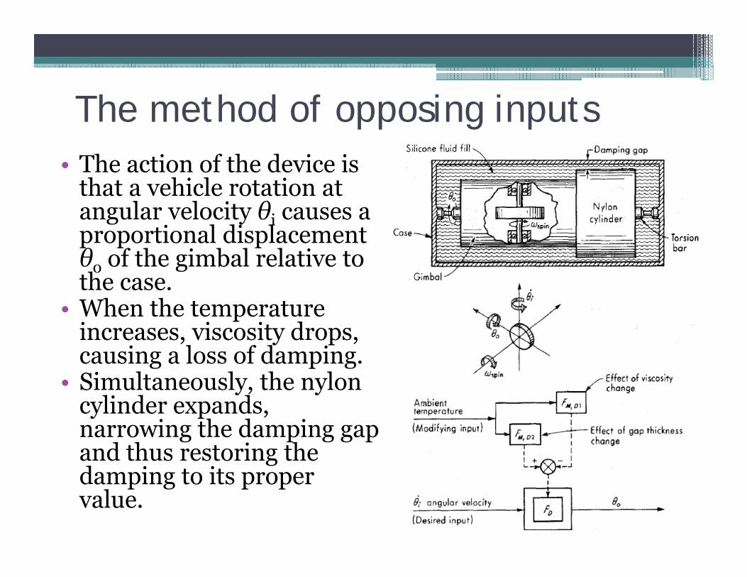
The method of opposing inputs• The action of the device is

that a vehicle rotation at angular velocity θi causes a proportional displacement θo of the gimbal relative to the case.

• When the temperature increases, viscosity drops, causing a loss of damping.

• Simultaneously, the nylon cylinder expands, narrowing the damping gap and thus restoring the damping to its proper value.

Measurement SystemsLecture 4- Generalized Performance Characteristics of Instruments


INTRODUCTION• Study the performance of measuring instruments

and systems with regard to: ▫ how well they measure the desired inputs, and▫ how thoroughly they reject the spurious inputs.

• The treatment of instrument performance characteristics is broken down into the subareas of▫ static characteristics, and ▫ dynamic characteristics.

• The overall performance of an instrument is then judged by a semi-quantitative superposition of the static and dynamic characteristics.

Static Characteristics and Static Calibration• Meaning of Static Calibration• Measured Value versus True

Value• Some Basic Statistics• Least-Squares Calibration Curves• Calibration Accuracy versus

Installed Accuracy• Combination of Component

Errors in Overall System-Accuracy Calculations

• Theory Validation by Experimental Testing

• Effect of Measurement Error on Quality Control Decisions in Manufacturing

• Static Sensitivity• Computer-Aided Calibration

and Measurement: Multiple Regression

• Linearity• Threshold, Noise Floor,

Resolution, Hysteresis, and Dead Space

• Scale Readability• Span• Generalized Static Stiffness and

Input Impedance: Loading Effects

• Concluding Remarks on Static Characteristics

Meaning of Static Calibration

• Static calibration : ▫ all inputs (desired, interfering, modifying) except

one are kept constant.▫ the input-output relations is developed

• Superposition of these individual effects describes the overall instrument static behavior.

• The calibration system should have a total uncertainty four times better than the unit under test.

Meaning of Static Calibration• In performing a calibration, the following steps are

necessary:▫ Examine the construction of the instrument, and

identify and list all the possible inputs.▫ Decide, as best you can, which of the inputs will be

significant in the application for which the instrument is to be calibrated.

▫ Procure apparatus that will allow you to vary all the significant inputs over the ranges considered necessary. Procure standards to measure each input.

▫ By holding some inputs constant, varying others, and recording the output(s), develop the desired static input-output relations.

Measured Value versus True Value

• The term "true value" refers to a reference value that would be obtained if the quantity under consideration were measured by an exemplar method;▫ a method agreed on by experts as being sufficiently

accurate for the purposes to which the data ultimately will be put.

• If measurement process is repeated under assumed identical conditions, we get a number of readings from the instrument;▫ the process must be in a state of statistical control


• Every instrument has an infinite number of inputs;

• In a calibration procedure, certain inputs are held "constant" within certain limits.

• These inputs contribute the largest components to the overall error of the instrument.

• The remaining infinite number of inputs is left uncontrolled, and it is hoped that each of these individually contributes only a very small effect

• In the aggregate these effect on the instrument output will be of a random nature.


• Effect of uncontrolled input on calibration• A measurement process with good statistical

control generates a set of data exhibiting random scatter.

Performing the calibration in a temperature-controlled room

Calibration was carried out without temperature control.

Some Basic Statistics

• Pressure-gage calibration data

Some Basic Statistics• Histogram presentation:

•The area of a particular "bar" is numerically equal to the probability that a specific reading will fall in the associated interval. •The area of the entire histogram must then be 1.0

Some Basic Statistics

• In limit with infinite number of readings, each with an infinite number of significant digits, Z = f(x) is called the probability density function.

Probability of reading lying between a and b

The cumulative distributionfunction

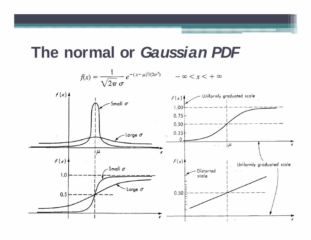
The normal or Gaussian PDF

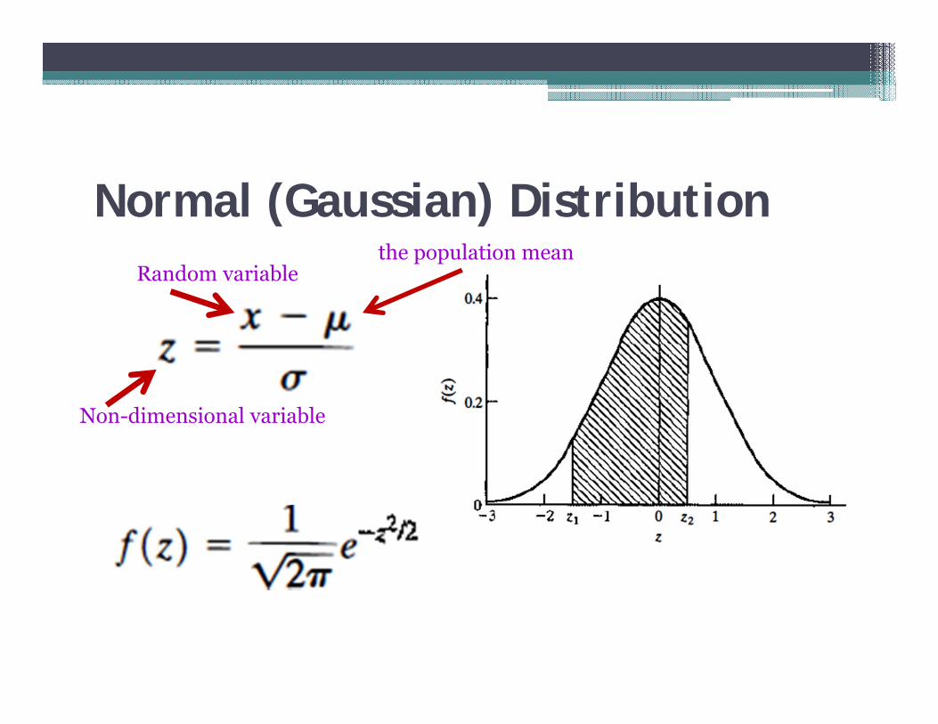
Normal (Gaussian) Distribution

Non-dimensional variable

Random variablethe population mean

Clearance deviations• Consider a shaft in a bearing DS=25.400 mm, and DB=25.451 mm. The

standard deviation of the shaft diameter is 0.008 mm, and the standard deviation of the bearing diameter is 0.010 mm. For satisfactory operation the difference in diameters (clearance) between the bearings must be between 0.0381 mm and 0.0635 mm. What fraction of the final assemblies will be rejected?

2 2

25.451 25.400 0.051

0.008 0.010 0.01280.0635 0.03810.98, 1.01

c

c c

C mm

S mmC C

S S

Mean Value

STD

Clearance deviationsConsidering C follows a Gaussian distribution 68.2% of products are accepted.The remaining are rejected.

Qualitative test for conformity to the Gaussian distribution

To plot Gaussian line, one must estimate

The effect of sample size increasing

• When real distribution is nearly Gaussian, if more readings were taken, 99.7 percent would fall within 10.11 ± 0.42 kPa

Display an empirical quantile-quantileplot

Student's t Distribution• Continuous, symmetrical distribution, used for

analysis of the variation of sample mean value for experimental data with sample size less than 30.▫ If the sample size is small (n < 30), the assumption

that the population standard deviation can be represented by the sample standard deviation may not be accurate.

▫ Due to the uncertainty in the standard deviation, for the same confidence level, we would expect the confidence interval to be wider.

• For sample sizes greater than 30, Student's t approaches normal distribution.

Student's t Distribution• In case of small samples, a statistic called

Student's t is used: the sample mean

the sample standard deviation

the sample size

degrees of freedomGamma function

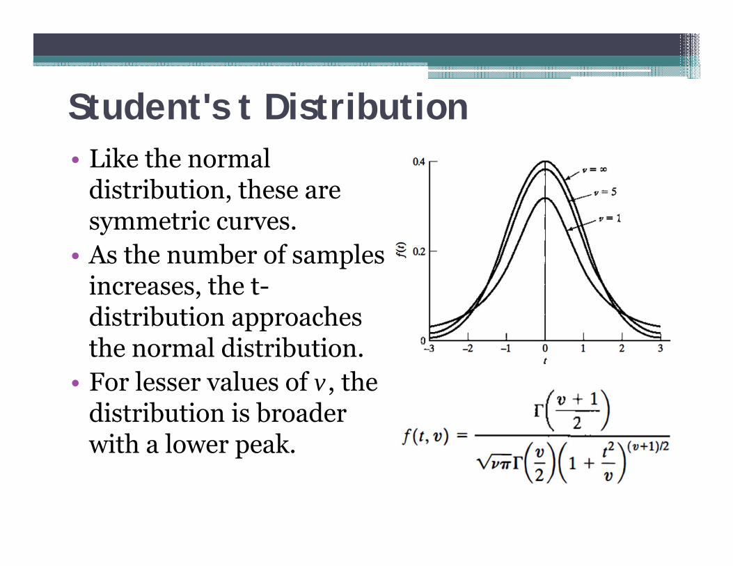
Student's t Distribution• Like the normal

distribution, these are symmetric curves.

• As the number of samples increases, the t-distribution approaches the normal distribution.

• For lesser values of v, the distribution is broader with a lower peak.

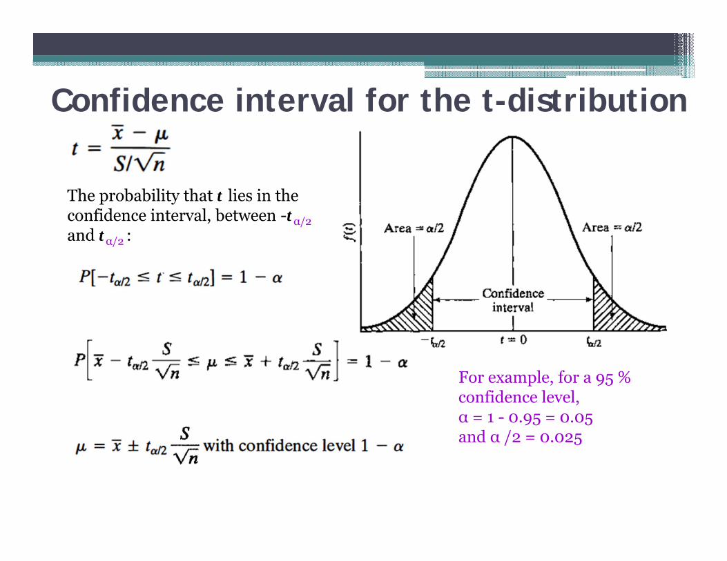
Confidence interval for the t-distribution

For example, for a 95 % confidence level, α = 1 - 0.95 = 0.05 and α /2 = 0.025

The probability that t lies in the confidence interval, between -tα/2and tα/2 :

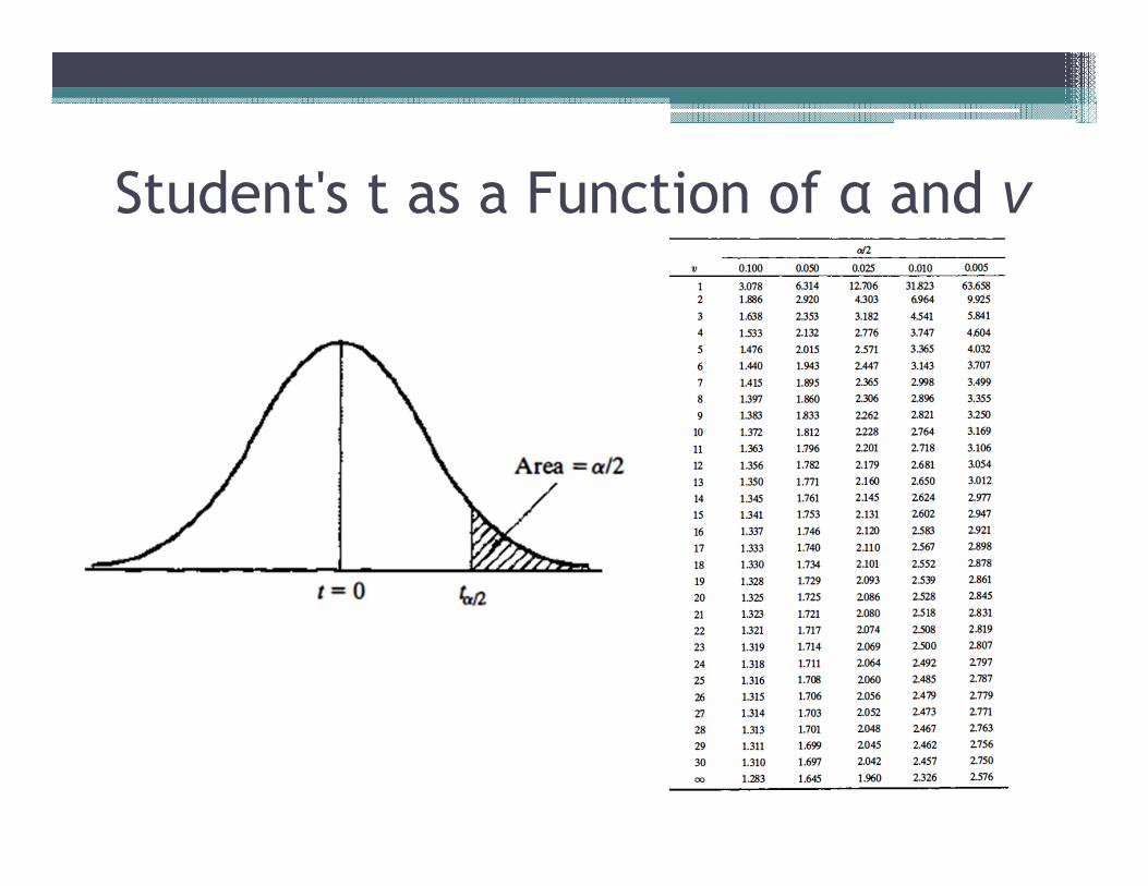
Student's t as a Function of α and v

Example : • A manufacturer would like to estimate the mean failure

time of its products with 95% confidence. Six systems are tested to failure, and the following data (in hours of functioning time) are obtained: 1250, 1320, 1542, 1464, 1275, and 1383. Estimate the population mean and the 95% confidence interval on the mean.

If we were to increase the confidence level, the estimated interval will also expand, and vice versa.

Interval Estimation of the Population Variance• In many situations, the variability of the random

variable is as important as its mean value. • The best estimate of the population variance, σ2,

is the sample variance, S2.• …….

Measurement SystemsLecture 5-Least-Squares Calibration Curves


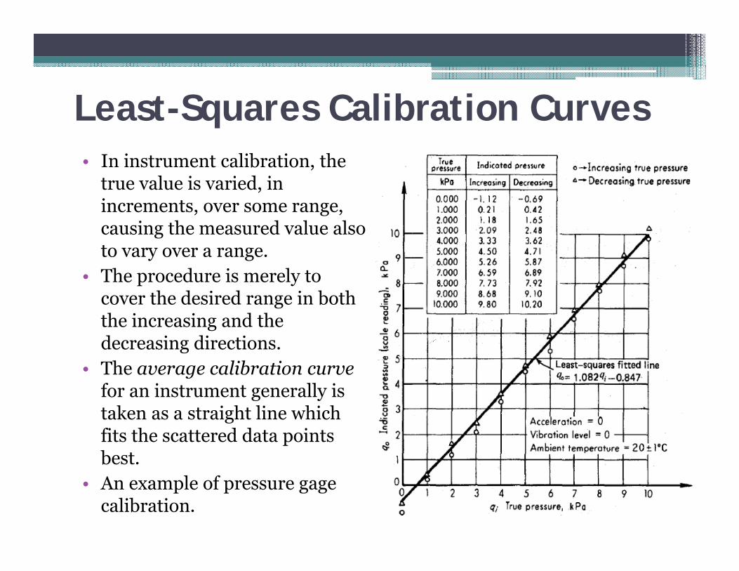
Least-Squares Calibration Curves• In instrument calibration, the

true value is varied, in increments, over some range, causing the measured value also to vary over a range.

• The procedure is merely to cover the desired range in both the increasing and the decreasing directions.

• The average calibration curve for an instrument generally is taken as a straight line which fits the scattered data points best.

• An example of pressure gage calibration.

Least-Squares Calibration Curves

⋮111⋮ ⋮1, x

Least-Squares Calibration Curves

x =1.0823

-0.8470

Least-Squares Calibration Curves• The model parameters are derived from scattered

data; it would be useful to have some idea of their possible variation:

• The standard deviation of q0 ,

▫ if qi were fixed and then repeated measurement of qo would give scattered values,

• The standard deviations of m and b may be found from:

Least-Squares Calibration Curves• Assume sqowould be the same for any value of qi,

= 0.208 kPa, = 0.0140 and = 0.0830 kPa• Assuming a Gaussian distribution and the 99.7

percent limits ( ± 3s), m= 1.082 ± 0.042 ,b=-0.847 ± 0.249

• The least-squares line gives:

• The qi value computed in this way must have some error limits put on it

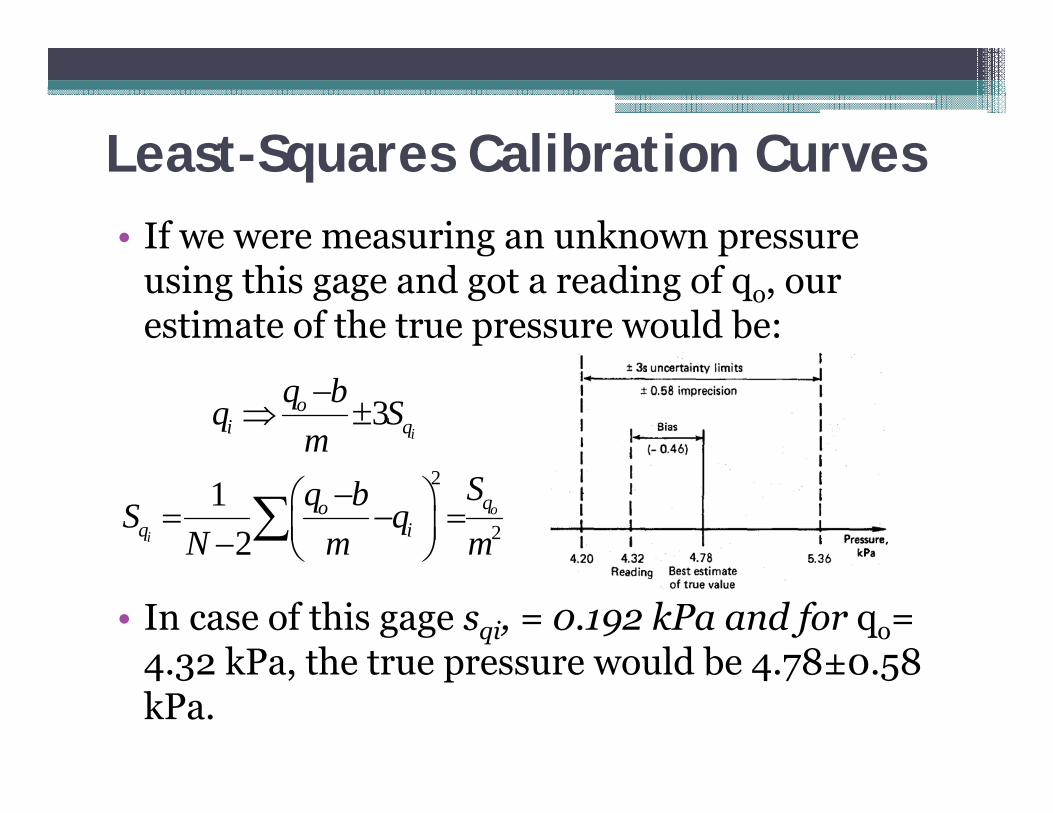
Least-Squares Calibration Curves• If we were measuring an unknown pressure

using this gage and got a reading of qo, our estimate of the true pressure would be:

• In case of this gage sqi, = 0.192 kPa and for qo= 4.32 kPa, the true pressure would be 4.78±0.58 kPa.

2

2

3

12

i

o

i

oi q

qoq i

q bq Sm

Sq bS qN m m

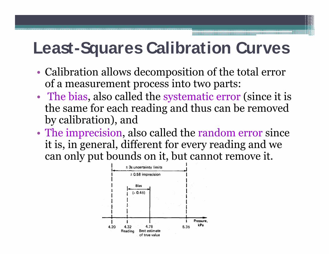
Least-Squares Calibration Curves• Calibration allows decomposition of the total error

of a measurement process into two parts:• The bias, also called the systematic error (since it is

the same for each reading and thus can be removed by calibration), and

• The imprecision, also called the random error since it is, in general, different for every reading and we can only put bounds on it, but cannot remove it.

Uncertainty Calculation using t-Distribution• Improvements with two major features: ▫ A simple method considers a standard deviation

calculated from a small number of points to be as accurate as one gotten from a large number of points. Statistical theory (confidence intervals) allows us to

adjust the uncertainty to suit the number of points.▫ The second improvement substitutes for our 3s

limits (99.7 percent level) a limit analogous to 2s (95 percent level).

Uncertainty Calculation using t-Distribution• For Gaussian and near-

Gaussian distributions, 99.7 percent puts us well into the "tails" of the distribution.▫ it takes very large samples to

get reliable results for probabilities

• Since most engineering samples are relatively small, quoting uncertainty bands at the 95 percent level of confidence is more realistic

Uncertainty Calculation using t-Distribution• Mandel gives a ± 95 percent confidence

interval, defined by two hyperbolas on either side of the least-squares line.

• The "vertical" location of the two hyperbolas as a function of qi is computed from:

N-2

t distribution values for uncertainty calculation

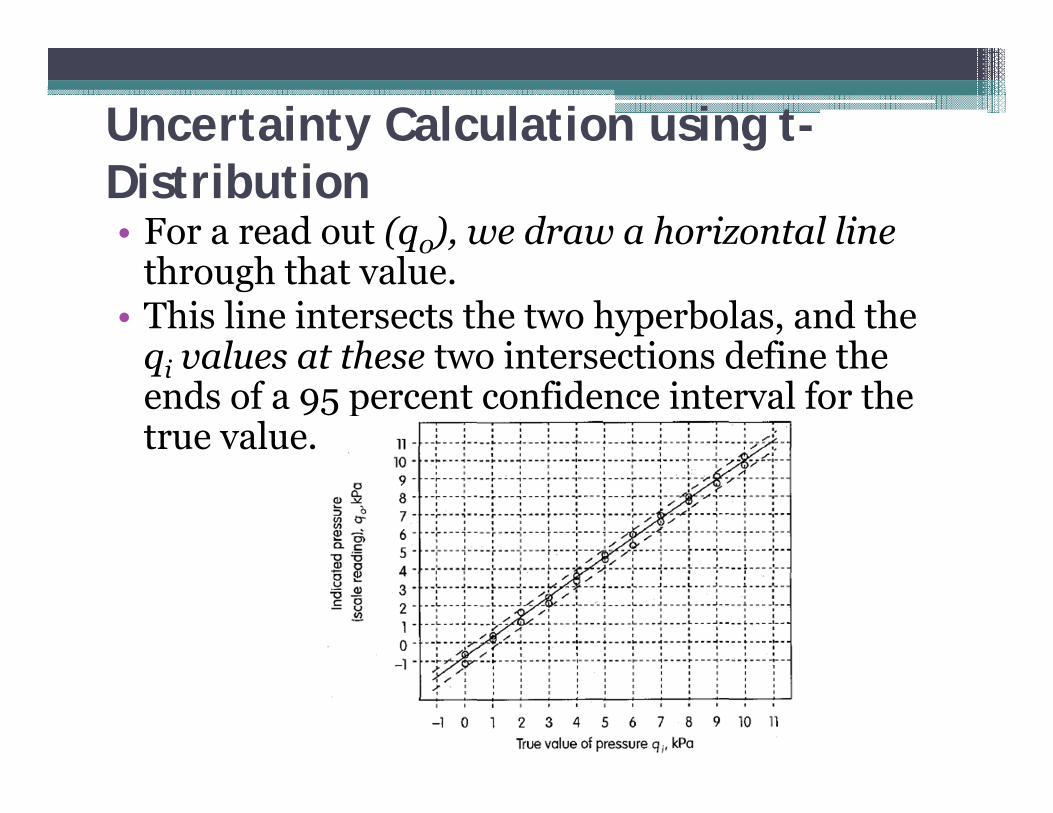
Uncertainty Calculation using t-Distribution• For a read out (q0), we draw a horizontal line

through that value. • This line intersects the two hyperbolas, and the

qi values at these two intersections define the ends of a 95 percent confidence interval for the true value.

Uncertainty Calculation using t-Distribution• Visually, the two "hyperbolas" seem to be

straight lines, but inspection of the tabular results shows that Δq0 does vary with qi▫ the largest value being at the left and right ends of

the curves and the smallest being at the center.

Uncertainty Calculation using t-Distribution• A major assumption of the analysis is that the statistical

variability of the measurements is the same over the entire calibration range.

• It is good practice to also make a plot of the residuals versus qi;▫ Such a graph can show whether this assumption is reasonable.

• For our example, shows no obvious trend in the size of the residuals; the variability seems to be about the same over the whole range.

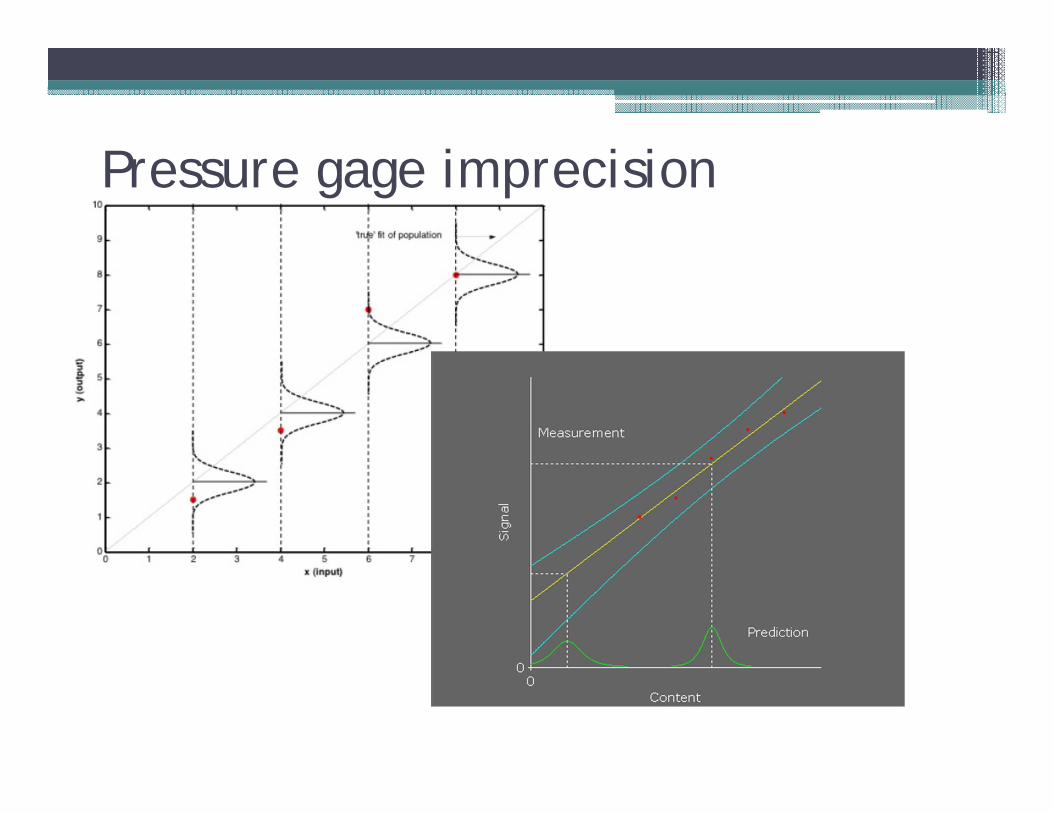
Pressure gage imprecision

• The average calibration curve for a pressure gage is

• For qo= 4.320 kPa, what is the best estimate of the true pressure?

• Calculate the imprecision in the estimation of input pressure with the 95% confidence interval.

0 01.0823 0.8470, 0.208iq q Sq kPa

0.8470 4.6911.0823

oi

qq kPa

0.2082 4.691 2 4.691 0.3841.0823i iq Sq kPa

4.307 5.075


qo= 4.320

4.307-5.075

Pressure gage imprecision• A 95 percent confidence interval can be defined by two hyperbolas on either

side of the least-squares line where the "vertical" location of the two hyperbolas as a function of qi is computed from:

• Calculate for the pressure gage when the input pressure is 5 kPa. Note: The experiments is repeated twice (n=2).

• At which input pressure(s) is maximized?

oq oq

oq

1 122, 2.086 0.208 0. 0.322 22oN q kPa

oq

@ 0. & 10kPa

Measurement SystemsLecture 6- Calibration Accuracy/ Overall System-Accuracy Calculations


Calibration Accuracy versus Installed Accuracy• It was stated that calibration removes the bias

portion of the error, • This is true only for the conditions under which the

calibration was performed:▫ This means that the measurement error (bias and

imprecision) must be re-evaluated, taking into account, as best possible, the deviation of the measurement conditions from the calibration conditions.

▫ This re-evaluation is usually not as straightforward as the calibration was because the measurement environment is rarely as controlled as a standards laboratory calibration.

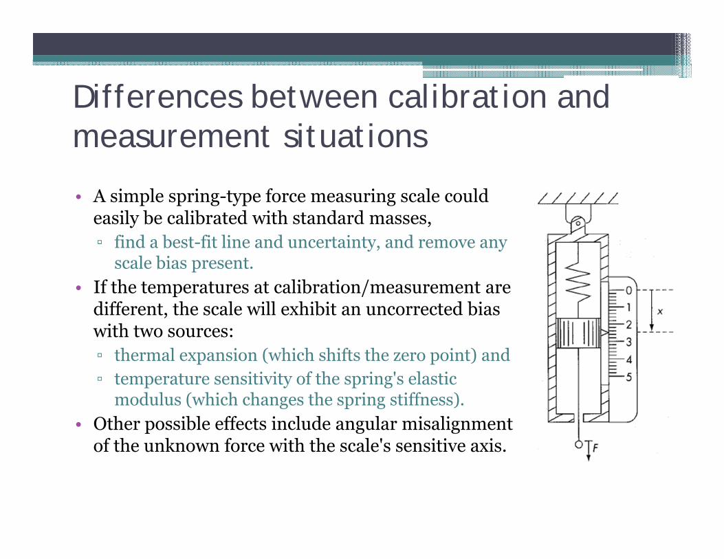
Differences between calibration and measurement situations

• A simple spring-type force measuring scale could easily be calibrated with standard masses,▫ find a best-fit line and uncertainty, and remove any

scale bias present.• If the temperatures at calibration/measurement are

different, the scale will exhibit an uncorrected bias with two sources:▫ thermal expansion (which shifts the zero point) and ▫ temperature sensitivity of the spring's elastic

modulus (which changes the spring stiffness).• Other possible effects include angular misalignment

of the unknown force with the scale's sensitive axis.

Calibration Accuracy versus Installed Accuracy• One aspect of the measurement situation is that the bias

portion of the error is now not zero. (Recall that we earlier said that calibration removes the bias.)

• Biases are classified into five different types:▫ Large known biases (eliminated by calibration).▫ Large unknown biases(not correctable; usually come from

human errors in data processing, incorrect installation and/or handling of instrumentation, and unexpected environmental disturbances). In a well-controlled measurement process, the assumption is that

there are no large unknown biases.▫ Small known biases (may or may not be corrected, depending

on the correction difficulty and their magnitude.).▫ Small unknown biases with unknown algebraic sign.▫ Small unknown biases with known algebraic sign.

Calibration Accuracy versus Installed Accuracy

• Small, unknown biases remain as a contribution to the measurement error.

• The bias in the measurement situation (as contrasted with calibration) is treated as a random effect rather than as systematic ▫ Bias limit: It is defined as the range of values within

which we feel that the actual bias will be found 95 percent of the time.

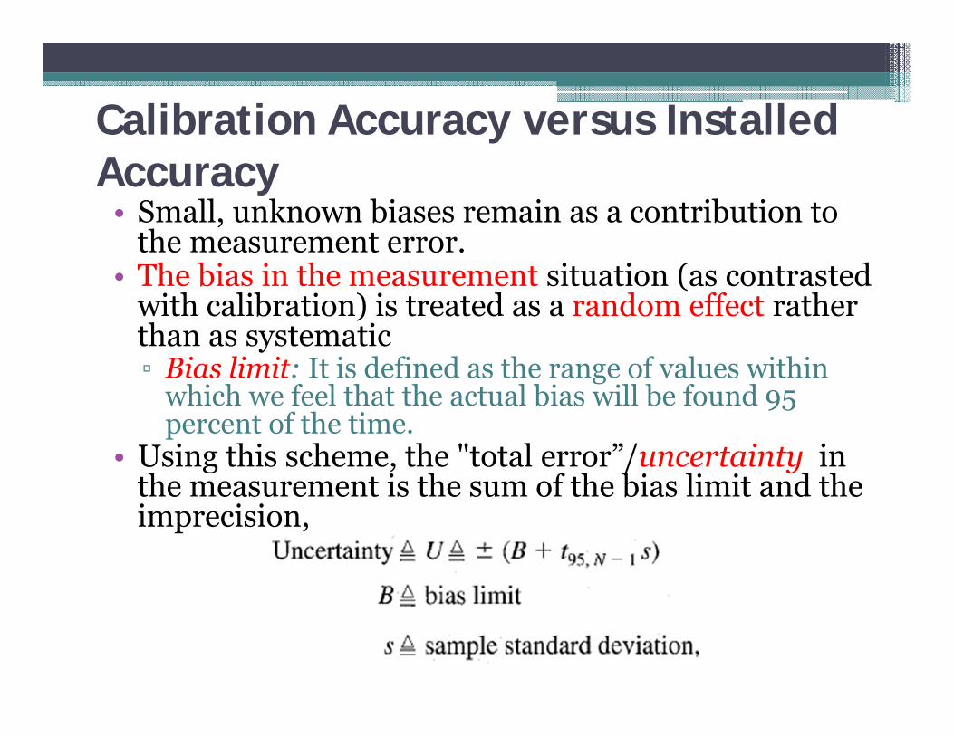
• Using this scheme, the "total error”/uncertainty in the measurement is the sum of the bias limit and the imprecision,

Calibration Accuracy versus Installed Accuracy

• To compute uncertainty in force measuring scale , we need to estimate the temperature, misalignment, and any other effects felt to be significant.

• Note that: ▫ we do not measure the temperature

and misalignment and then correct for these effects, rather

▫ we estimate some limits on how large we think these effects might be and then add this to the uncertainty.

Calibration Accuracy versus Installed Accuracy• A displacement-measuring dial indicator

as part of an experiment to find the beam's spring constant, F/δ.

• A bias error will be introduced because the indicator spring force acts against F, ▫ Causing the measured deflection to be less

than it should be. ▫ If F is always downward, this bias error

would be treated as having an unknown magnitude, but a known sign.

▫ The deflection is always measured too low. • If we estimate an upper limit for its

magnitude, this bias would give an unsymmetrical uncertainty; for example, -0.003 in. to +0.001 in.

Calibration Accuracy versus Installed Accuracy• Thermocouples are calibrated in an

accurately controlled and measured temperature environment.▫ The wires are immersed in a liquid-filled

well whose temperature is uniform at Thotover a long distance to prevent conduction heat transfer along the wires, which would cause the sensing tip to read too low.

• When used to measure the temperature of a hot gas, the wires are in contact with a cool duct wall, conduction is now not negligible, and the sensing tip will read low.

Calibration Accuracy versus Installed Accuracy• If such an error causes unacceptable

uncertainty, we may measure the wall temperature, estimate the needed heat transfer parameter, and compute a correction.

• This correction will improve the uncertainty, but not eliminate it, since the correction will itself be uncertain, which uncertainty we will have to estimate and include.

• For example, if our reading is 357°C and, ▫ the correction is +8°C, the nominal value is

365°C. ▫ If the uncertainty in the correction is±2°C,

and the uncertainty due to other sources was ±5°C, the temperature would be quoted as 365±7°C.

Calibration Accuracy versus Installed Accuracy• In situ calibration, if possible, would in many cases be preferred, ▫ the calibration numerical results would include all the effects

contributing to uncertainty ▫ not require separate judgments and estimates based on experience

rather than actual measured data.• In a similar spirit, we should also consider the end-to-end

calibration.▫ rather than calibrating separately each link (sensor, amplifier, filter,

recorder, etc.) in our measurement chain and then combining the individual uncertainties mathematically, we apply a standard to only the sensor input and record only the final output.

▫ Advantage :all interactions among the links are automatically taken into account and the procedure may be considerably quicker.

▫ Disadvantage: we do not see which components are contributing the most to the total uncertainty.

▫ Even when we do perform the individual calibrations, a final end-to-end study may be desirable.

Combination of Component Errors in Overall System-Accuracy Calculations• A measurement system is often made up of a chain

of components, each of which is subject to individual (known) inaccuracy.

• How is the overall inaccuracy computed?• If the Δx's are now considered to be the

uncertainties uxi in each measured value xi, then the corresponding uncertainty Uy in y is

Combination of Component Errors in Overall System-Accuracy Calculations• Think of the partial derivative as the sensitivity

of y to changes in the particular x.

▫ when a partial derivative has a large numerical value, y is very sensitive to that particular x.

• The partial derivatives are numerically evaluated at the operating point, ▫ they are constants (not functions), so this

equation defines y as a linear function of the x's, even though the original function (f) may be nonlinear.

Combination of Component Errors in Overall System-Accuracy Calculations• This relation is called the root-sum-square (rss)

formula,

• We have not here proven its validity, but this rests on the fact that the standard deviation of any linear function of Gaussian independent variables is given by the square root of the sum of squares of the individual standard deviations.

• It is an approximate result because y is not really a linear function of the x's; it is close to linear only for small changes.

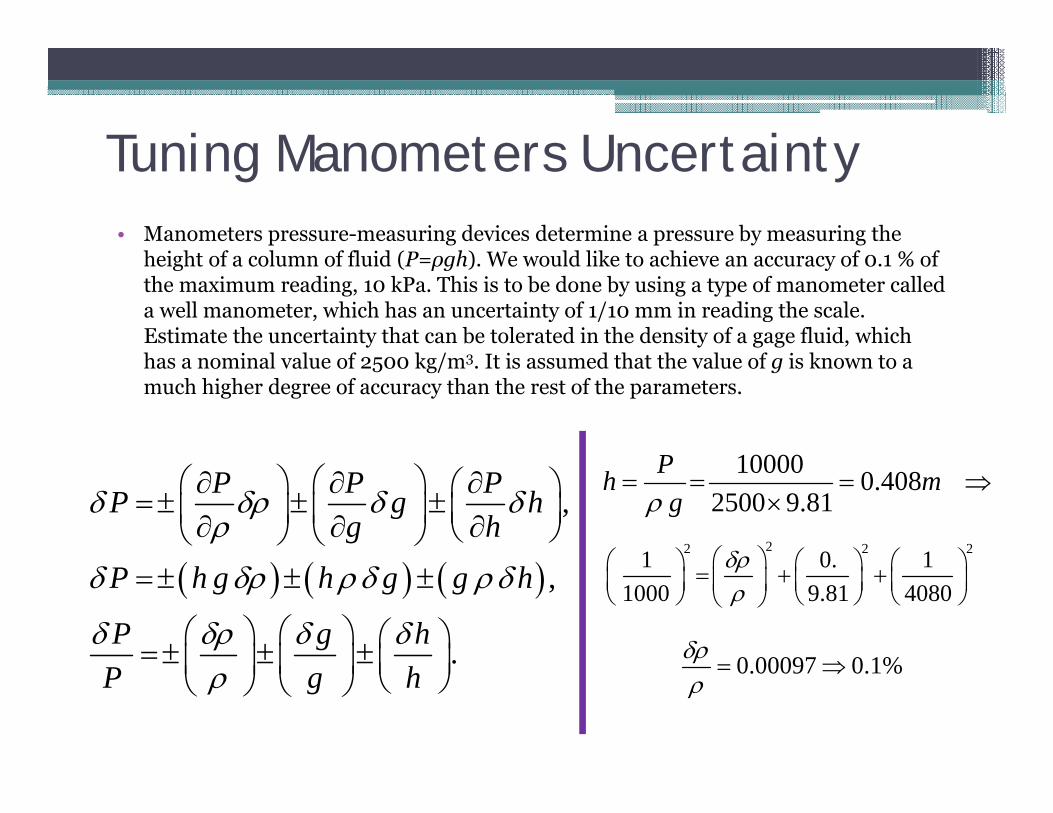
Tuning Manometers Uncertainty • Manometers pressure-measuring devices determine a pressure by measuring the

height of a column of fluid (P=ρgh). We would like to achieve an accuracy of 0.1 % of the maximum reading, 10 kPa. This is to be done by using a type of manometer called a well manometer, which has an uncertainty of 1/10 mm in reading the scale. Estimate the uncertainty that can be tolerated in the density of a gage fluid, which has a nominal value of 2500 kg/m3. It is assumed that the value of g is known to a much higher degree of accuracy than the rest of the parameters.

22 2 21 0. 11000 9.81 4080

10000 0.4082500 9.81

Ph mg

0.00097 0.1%

,

,

.

P P PP g hg h

P h g h g g h

P g hP g h

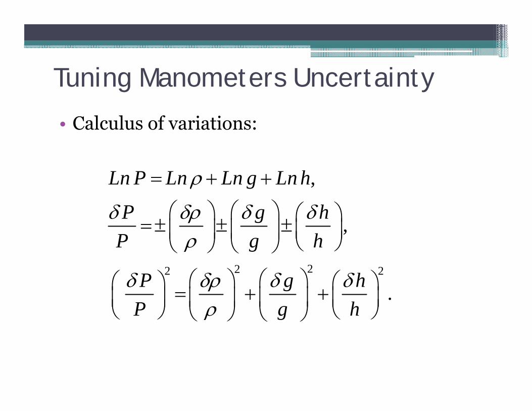
Tuning Manometers Uncertainty

• Calculus of variations:

222 2

,

,

.

Ln P Ln Ln g Ln h

P g hP g h

P g hP g h

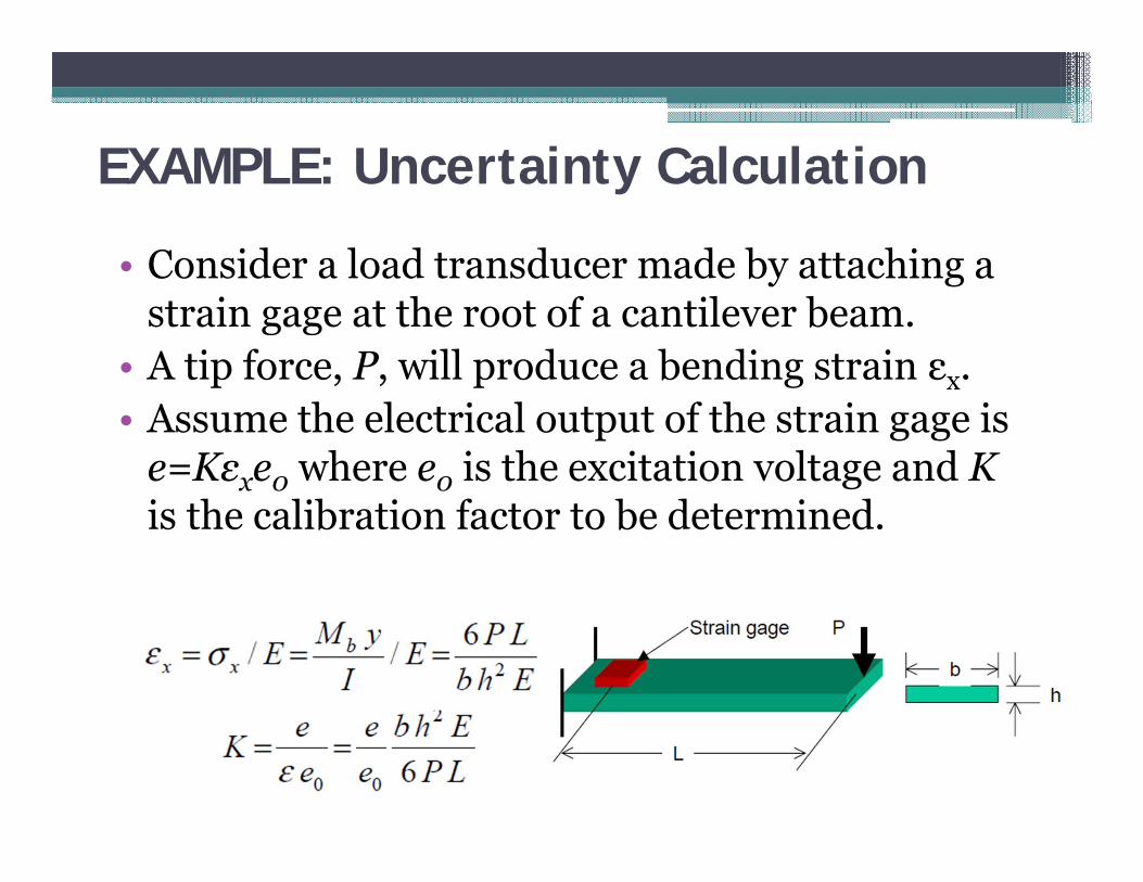
EXAMPLE: Uncertainty Calculation

• Consider a load transducer made by attaching a strain gage at the root of a cantilever beam.

• A tip force, P, will produce a bending strain εx.• Assume the electrical output of the strain gage is

e=Kεxe0 where e0 is the excitation voltage and Kis the calibration factor to be determined.

Uncertainty Calculation

1/222 2 2 2 2 2

00

K K K K K K KK e e b h E P Le e b h E P L

1/222 2 2 2 2 20

0

2eK e b h E P LK e e b h E P L


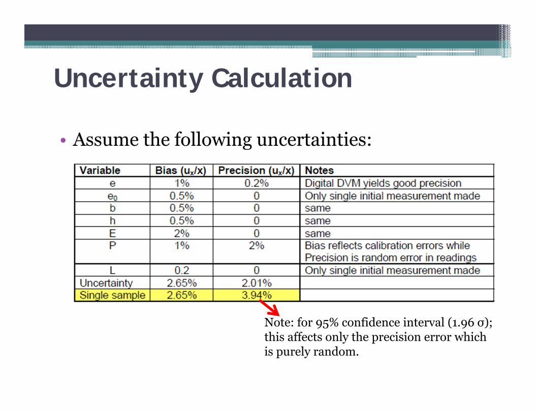
• Assume the following uncertainties:

Note: for 95% confidence interval (1.96 σ);this affects only the precision error which is purely random.


• Total uncertainty in the measurement of K is then:

1/22 2

1/22 22.65 3.94 % 4.75%

bias precisionK U U

K

measurement · pdf filewhy study measurement systems? • in design stage, ... functional...

Documents