measurement of quartic boson couplings at the
TRANSCRIPT

Measurement of quartic boson couplings atthe international linear collider and study
of novel particle flow algorithms
Dissertationzur Erlangung des Doktorgrades
des Fachbereichs Physikder Universitat Hamburg
vorgelegt vonPredrag Krstonosic
HamburgFebruar 2008

Gutachter der Dissertation : Prof. Dr. R.-D. HeuerProf. Dr. P. Schleper
Gutachter der Disputation : Prof. Dr. R.-D. HeuerProf. Dr. P. Schleper
Datum der Disputation : 22.02.2008
Vorsitzender des Prufungsausschusses : Dr. K. Petermann
Vorsitzender des Promotionsausschusses : Prof. Dr. G. Huber
MIN-Dekan des Department Physik : Prof. Dr. A. Fruhwald

“Reality has to take precedence over Public Relations, for Nature cannot be fooled!”
Richard Feynman
“We don’t want most beautiful and most abstract software, but one that works!”
Ties Behnke

Acknowledgments
First of all I want to thank to Klaus Monig for providing plesent atmosphere from my firstday in the Deutschen Electronen-Synchrotron (DESY) and for years of fruitfull work together.
Also, I would like to thank Wolfgang Kilian and Jurgen Reuter for relieble guidence throughthe dungines of theory. Special thank to Vasilly Morgunov for refreshing and usefull discuss-sions that have deepen my insigt in many subjects.
Thank to all the unmentioned peopele that have succeded to improove my mood on coloudydays. At the end my sincere condolence to all those forced to read this text, since I’m muchbetter at calculating then writing.

Abstract
In the absence of the Standard Model Higgs boson the interaction among the gaugebosons becomes strong at thigh energies (∼ 1TeV ) and influences couplings between them.Trilinear and quartic gauge boson vertices are characterized by set of couplings that areexpected to deviate from Standard Model at energies significantly lower then the energy scaleof New Physics. Estimation of the precision with which we can measure quartic couplingsat International Linear Collider (ILC) is one of two topics covered by this theses. There areseveral measurement scenarios for quartic couplings. One that we have chosen is weak bosonscattering. Since taking of the real data is, unfortunately, still far in the future runningoptions for the machine were also investigated with their impact on the results. Analysiswas done in model independent way and precision limits were extracted. Interpretationof the results in terms of possible scenarios beyond Standard Model is then performed bycombining accumulated knowledge about all signal processes. One of the key requirements foracheaving the results of the measurement in the form that is presented is to reach the detectorperformance goals. This is possible only with “Particle Flow” reconstruction approach.Performance limit of such approach and various contribution to it will be discussed in detail.Novel reconstruction algorithm for photon reconstruction is developed, and performancecomparison of such concept with more traditional approaches is done.

Zusammenfassung
Ohne das Higgs Boson des Standardmodells wird die Wechselwirkung der Eichbosonen beiEnergien um 1 TeV stark und beeinflusst die Kopplung zwischen ihnen. Trilineare und biqua-dratische Eichbosonvertices werden durch einen Satz Kopplungen charakterisiert. Von diesemwird erwartet, dass er von dem des Standardmodells, bei Energien die deutlich unterhalb derSkala neuer Physik liegen, abweicht. Eines der beiden Themen dieser Doktorarbeit ist dieAbschatzung der Prazision, mit der biquadratische Kopplungen am Internationalen Linear-beschleuniger (ILC) gemessen werden konnen. Es gibt mehrere mogliche Szenarien, in derenRahmen biquadratische Kopplungen gemessen werden konnen. Es wurde das Szenario mitschwacher Boson Streuung gewahlt. Da die tatsachliche Datennahme noch weit in der Zu-kunft liegt, wird auch der Einfluss verschiedener Betriebsmoglichkeiten des Beschleunigers aufdieses Ergebnis getestet. Die Analyse wurde Modellunabhangig ausgefuhrt, und die Grenzender Prazision wurden bestimmt. Bei der Deutung der Ergebnisse in Hinblick auf moglichePhysik jenseits des Standardmodells wurden alle Signalprozesse berucksichtigt. Um die Mess-ergebnisse in der dargestellten Form zu erreichen, muss die angestrebte Detektorleistung erfulltwerden. Dies ist nur unter Verwendung des Particle FlowAnsatzes machbar. Die Grenzen ei-nes solchen Ansatzes, sowie verschiedene Einfusse auf diese, werden im Detail untersucht. Einneuer Rekonstruktionsalgorhythmus fur Photonen wird entwickelt und mit konventionellerenAnsatzen verglichen.


Contents
1 Introduction 11.0.1 Outline of the theses . . . . . . . . . . . . . . . . . . . . . . . . . . . . . 2
2 International Linear Collider (ILC) 32.0.2 Accelerator . . . . . . . . . . . . . . . . . . . . . . . . . . . . . . . . . . 3
2.1 Detector . . . . . . . . . . . . . . . . . . . . . . . . . . . . . . . . . . . . . . . . 42.1.1 Tracking system . . . . . . . . . . . . . . . . . . . . . . . . . . . . . . . 52.1.2 Electromagnetic calorimeter . . . . . . . . . . . . . . . . . . . . . . . . . 92.1.3 Hadronic calorimeter . . . . . . . . . . . . . . . . . . . . . . . . . . . . . 102.1.4 Muon system . . . . . . . . . . . . . . . . . . . . . . . . . . . . . . . . . 112.1.5 Forward region . . . . . . . . . . . . . . . . . . . . . . . . . . . . . . . . 112.1.6 Detector design evolution . . . . . . . . . . . . . . . . . . . . . . . . . . 12
3 Quartic couplings 153.1 Standard Model . . . . . . . . . . . . . . . . . . . . . . . . . . . . . . . . . . . . 15
3.1.1 Electroweak sector . . . . . . . . . . . . . . . . . . . . . . . . . . . . . . 193.1.2 Symmetry breaking sector . . . . . . . . . . . . . . . . . . . . . . . . . . 21
3.2 Effective Lagrangian . . . . . . . . . . . . . . . . . . . . . . . . . . . . . . . . . 243.3 Measurement strategy . . . . . . . . . . . . . . . . . . . . . . . . . . . . . . . . 263.4 Resonances . . . . . . . . . . . . . . . . . . . . . . . . . . . . . . . . . . . . . . 28
3.4.1 Scalar singlet . . . . . . . . . . . . . . . . . . . . . . . . . . . . . . . . . 283.4.2 Scalar triplet . . . . . . . . . . . . . . . . . . . . . . . . . . . . . . . . . 293.4.3 Scalar quintet . . . . . . . . . . . . . . . . . . . . . . . . . . . . . . . . . 293.4.4 Vector singlet . . . . . . . . . . . . . . . . . . . . . . . . . . . . . . . . . 303.4.5 Vector triplet . . . . . . . . . . . . . . . . . . . . . . . . . . . . . . . . . 313.4.6 Tensor singlet . . . . . . . . . . . . . . . . . . . . . . . . . . . . . . . . . 323.4.7 Tensor triplet . . . . . . . . . . . . . . . . . . . . . . . . . . . . . . . . . 323.4.8 Tensor quintet . . . . . . . . . . . . . . . . . . . . . . . . . . . . . . . . 33
4 Analysis and Results 354.1 Direct measurement of quartic couplings . . . . . . . . . . . . . . . . . . . . . . 35
4.1.1 Processes . . . . . . . . . . . . . . . . . . . . . . . . . . . . . . . . . . . 354.1.2 Observable . . . . . . . . . . . . . . . . . . . . . . . . . . . . . . . . . . 36
4.2 Event selection . . . . . . . . . . . . . . . . . . . . . . . . . . . . . . . . . . . . 374.2.1 Jet pairing . . . . . . . . . . . . . . . . . . . . . . . . . . . . . . . . . . 374.2.2 B tagging . . . . . . . . . . . . . . . . . . . . . . . . . . . . . . . . . . . 414.2.3 Forward region . . . . . . . . . . . . . . . . . . . . . . . . . . . . . . . . 424.2.4 Overview of selection criteria . . . . . . . . . . . . . . . . . . . . . . . . 44
4.3 Quartic couplings extraction . . . . . . . . . . . . . . . . . . . . . . . . . . . . . 48
iii

iv Chapter 0. CONTENTS
4.4 Quartic coupling limits . . . . . . . . . . . . . . . . . . . . . . . . . . . . . . . . 514.4.1 Combined results . . . . . . . . . . . . . . . . . . . . . . . . . . . . . . . 524.4.2 Running options . . . . . . . . . . . . . . . . . . . . . . . . . . . . . . . 54
4.5 Model dependent limits on new physics . . . . . . . . . . . . . . . . . . . . . . 564.5.1 Combination of measurements . . . . . . . . . . . . . . . . . . . . . . . 574.5.2 Mass limit extraction . . . . . . . . . . . . . . . . . . . . . . . . . . . . 57
4.6 Mass limit results . . . . . . . . . . . . . . . . . . . . . . . . . . . . . . . . . . . 584.6.1 Scalar singlet . . . . . . . . . . . . . . . . . . . . . . . . . . . . . . . . . 584.6.2 Scalar triplet . . . . . . . . . . . . . . . . . . . . . . . . . . . . . . . . . 614.6.3 Scalar quintet . . . . . . . . . . . . . . . . . . . . . . . . . . . . . . . . . 624.6.4 Vector singlet . . . . . . . . . . . . . . . . . . . . . . . . . . . . . . . . . 654.6.5 Vector triplet . . . . . . . . . . . . . . . . . . . . . . . . . . . . . . . . . 664.6.6 Tensor singlet . . . . . . . . . . . . . . . . . . . . . . . . . . . . . . . . . 704.6.7 Tensor triplet . . . . . . . . . . . . . . . . . . . . . . . . . . . . . . . . . 724.6.8 Tensor quintet . . . . . . . . . . . . . . . . . . . . . . . . . . . . . . . . 73
4.7 Summary . . . . . . . . . . . . . . . . . . . . . . . . . . . . . . . . . . . . . . . 77
5 Particle flow 795.1 The concept of particle flow . . . . . . . . . . . . . . . . . . . . . . . . . . . . 79
5.1.1 Hardware parameters and Eflow reaches of LEP experiments . . . . . . 815.1.2 Jet energy resolution . . . . . . . . . . . . . . . . . . . . . . . . . . . . . 825.1.3 Contributions to the jet energy resolution . . . . . . . . . . . . . . . . . 84
5.2 Magnetic field effects . . . . . . . . . . . . . . . . . . . . . . . . . . . . . . . . . 875.2.1 Effects on calibration . . . . . . . . . . . . . . . . . . . . . . . . . . . . . 875.2.2 Effects on shower size . . . . . . . . . . . . . . . . . . . . . . . . . . . . 895.2.3 Effects on full reconstruction . . . . . . . . . . . . . . . . . . . . . . . . 91
5.3 Conclusion . . . . . . . . . . . . . . . . . . . . . . . . . . . . . . . . . . . . . . 93
6 Particle Reconstruction in ILC Detector 956.1 Approach to Reconstruction . . . . . . . . . . . . . . . . . . . . . . . . . . . . . 95
6.1.1 Reconstruction framework . . . . . . . . . . . . . . . . . . . . . . . . . . 956.1.2 Requirements for the electromagnetic shower reconstruction . . . . . . . 96
6.2 Electromagnetic Shower . . . . . . . . . . . . . . . . . . . . . . . . . . . . . . . 986.2.1 Longitudinal development . . . . . . . . . . . . . . . . . . . . . . . . . . 996.2.2 Transverse development . . . . . . . . . . . . . . . . . . . . . . . . . . . 100
6.3 Photon finding algorithm . . . . . . . . . . . . . . . . . . . . . . . . . . . . . . 1026.3.1 Algorithm steps . . . . . . . . . . . . . . . . . . . . . . . . . . . . . . . . 1026.3.2 Summary of steering parameters . . . . . . . . . . . . . . . . . . . . . . 1126.3.3 Algorithm performance . . . . . . . . . . . . . . . . . . . . . . . . . . . 1136.3.4 Conclusion . . . . . . . . . . . . . . . . . . . . . . . . . . . . . . . . . . 122
7 Summary and conclusions 125
A Theory addons 126A.0.5 groups . . . . . . . . . . . . . . . . . . . . . . . . . . . . . . . . . . . . . 127A.0.6 Goldston theorem . . . . . . . . . . . . . . . . . . . . . . . . . . . . . . 128
B Pflow factorization 130

C Summary of the formulae for photon shower parameterization 133C.1 Homogeneous media . . . . . . . . . . . . . . . . . . . . . . . . . . . . . . . . . 133
C.1.1 Average longitudinal profiles . . . . . . . . . . . . . . . . . . . . . . . . 133C.1.2 Average radial profiles . . . . . . . . . . . . . . . . . . . . . . . . . . . . 133
C.2 Sampling calorimeter . . . . . . . . . . . . . . . . . . . . . . . . . . . . . . . . . 134C.2.1 Material and geometry parameters . . . . . . . . . . . . . . . . . . . . . 134C.2.2 Average longitudinal profiles . . . . . . . . . . . . . . . . . . . . . . . . 134C.2.3 Average radial profiles . . . . . . . . . . . . . . . . . . . . . . . . . . . . 134
Bibliography 134


Chapter 1
Introduction
How it all began? All started on not so sunny day almost five years ago on the bus stop infront of the army base. I have accidentally 1 met aqventance of my, physicist understandably,and we have started a small talk. Just by the way I was informed about possibility for a jobat Institute for Nuclear Sciences Vinca in Belgrade. I have applied for the position and got it.The job implied leaving the real world of nuclear and medical physics and adjusting to the tobe world of future and beyond experiments, discoveries and theories. It was in the beginning“cultural shock”seeing and listening to the people that are talking “fairy tails”. In mean whileI have to some part also become a story teller but with, I hope, good dose of skepticism thatshould be noticeable through the theses. In the center of tail, we will tell, there is as highenergy e+e− collider. Under the Olympic motto (“Faster, Higher, Stronger”), it should leadus to the new stage of particle physics beyond the present day theory ( Standard Model (SM)).Electrons and positrons will be faster then ever before, it will provide higher precision of themeasurement and lead to the stronger constrains on the theory. Major objection to SM itis that the nature of mass, that is fundamental quantity in our system of units, is unknown.By Deus ex machina approach, solution for the masses within the theory is introduced andsearch for the holy grail of particle physics, Higgs particle, that this solution postulates hasbegun, so far without any success. In opinion on this subject one can aline himself with thebelievers expecting that the missing part will be observed, and non-believers that usually haveinteresting explanation of their own. As always when main hero becomes too arrogant andnarcistic story could have a turnover and the nature will have its final word. We will tryto follow the middle way starting with that what we know today and try to infer how ourknowledge would be expanded by measurement making as few assumption as possible. Thusinstead of rigid solution we can assume that the interactions that we observe are only low-energy approximations to the true mechanisms that work as some higher energy scale. Thisapproach is formalized in the Effective Lagrangian - low energy expansion of the true theory.Since one knows the expected values for the parameters of the Effective Lagrangian in case ofSM, any experimentally significant deviation from these values can give insight into underlyingtheory. One such subset of parameters are quartic couplings. There are several classes ofphysics processes in which such deviation could be observed. One chosen here is, so called,weak boson scattering. After measurement of the parameters one needs to make a consistentset of their values and then it is possible to discuss their meaning in terms of particular theorymodel. Trivially, but true, if you want to measure something you need the detector. Alleasy measurable things are already determined rather precisely and in order to make anotherstep one needs to increase the precision even further. This puts rather strict constrains on
1if such things exist at all
1

2 Chapter 1. Introduction
the needed luminosity and detector performance. Detector performance goal can be reachedwith new reconstruction method called Particle Flow, that is at the same time detector designguideline. Understanding the limitations of the method and essential contributions to theoverall performance is of great importance for the proper detector design and final physicsoutput. As even the best car is worth nothing without gasoline, so is the excellent detectorwithout matching reconstruction software. New detector concept requires development of newreconstruction methods that are of equal importance as underlying hardware. Unfortunatelysupport for the two branches that will lead us to the goal was highly disproportional, leeringsometimes to the, false, conclusion “that will not work”. Part of this story will be thusdedicated to shattering this doubts. Since it is already rather late, lets start.
1.0.1 Outline of the theses
Theses has two, apparently, disconnected parts measurement of quartic coupling and eval-uation and development of new reconstruction methods. It starts with introduction to theInternational Linear Collider (ILC), both accelerator and its detector in Chapter 2. Since de-tector used in the first part differs form the up to date design both detectors will be presentedin parallel stressing their differences. In Chapter 3 we shortly remind reader about standardmodel as a gauge theory, introduce Effective Lagrangian, introduce quartic couplings. In thesame chapter measurement strategy for the quartic couplings is presented as well as their rela-tion to possible new resonances at TeV scale. In Chapter 4 we will cover analiss part in termsof event selection and correct interpretation of the results. Essential steps in data treatmentare fully explained. Sensitivity limits for measurement are extracted and interpretation of theresults is done in terms of to be resonances. In Chapters 5 Particle Flow approach is discussedin some detail with clarification of most common misunderstandings. Personal contributionto reaching the detector design performance in form of photon reconstruction algorithm ispresented in Chapter 6 together with comparison of it’s performance with respect to othertools on the market. Finally, the results presented in this theses are summarized in Chapter7. Any material that might be useful for understanding of the text and has not fitted on otherplace is in appendix.

Chapter 2
International Linear Collider (ILC)
It is hard to escape from the historical approach in the introduction to the project that spansover so many years, but we will try to restrict ourself to the time span during which this theseswas done, for larger scope see [1]. During this time one was able to observe organization 1 ofthe global effort for the linear collider. Abrevation have changed from 3 letter ones to 4 andmore and International Linear Collider Steering Committee (ILCSC) subgroup on parametershas made two documents about project scope, one in 2003 [2] and in 2006 [3]. On the basesof these two documents we can say the following. The ILC baseline is an e+e− collider thatshould be able to reach a center of mass energy of 500GeV, and allow physics measurementsin the range of 200-500GeV. The Luminosity should be 2 × 1034cm−2s−1 at 500GeV andthe electron beam polarization of at least 80% within whole energy range used for physicsrunning. This would allow the collection of approximately Leq = 500fb−1 in the first fouryears of running. Beam energy stability should be below 10−3 level. There are tiny andnot essential differences between the two documents. One of them is that in 2003, “Twointeraction regions should be planned, with space and infrastructure for two experiments,with explanation. Two experiments are desired to allow independent measurement of criticalparameters and to provide better use of the beams thereby maximizing physics output. Atleast one of them should allow crossing angle with γγ interaction region”. That has changedto “The interaction region (IR) should allow for two experiments” with, interestingly, sameexplanation. Second is that “The maximum luminosity is not needed at the top energy(500GeV)...” , unfortunately without a reference, since this implies that one knows wherethe maximum is needed thus what physics scenario is realized in nature. All other possibleparameters of the project are considered as options beyond baseline. Those are energy upgradeup to 1TeV, positron polarization at or above 50% as well as the running in the e−e− mode.On the bases of these requirements there is a design that is supposed to fulfill them explainedin detail in ILC Reference Design Report [5]. We will just flash the accelerator with fewremarks here and there and discuss detector in some detail, specially those elements that areof interest for quartic boson couplings analysis and reconstruction.
2.0.2 Accelerator
The accelerator is based on a superconducting RF cavities on the recommendation of Inter-national Technical Recommendation Panel (ITRP) [4]. The average accelerating gradient incavities is supposed to be 31.5 MV/m. The current layout of the machine is in Fig.2.1. Anelectron source feeds the electron arm of the accelerator. A damping ring for electrons and
1reed birocratization
3

4 Chapter 2. International Linear Collider (ILC)
Figure 2.1: Layout of the ILC design.
positrons is placed centrally. The positrons source is undulator based and thus integratedin the electron arm of the main linac. One can note strange positioning of the detectors inthe middle of the layout. This is due to the fact that the proposal contains two detectors 2
but only one beam delivery system and interaction point (IP). The detectors will have timesharing of the beam by positioning one or another at the IP (push-pull design). As indicatedon the layout beams are not colliding head on but with the 14mrad crossing angle. Althoughsometimes neglected detail constructional and operating parameters of the accelerator willhave a significant impact on the detector-measurement performance beyond usually consid-ered parameters as center of mass energy and integrated luminosity. Due to this fact thereis a nominal set of beam and IP parameters containing variables like repetition rate of beampulses (5Hz), number of bunches per puls (2625), number of particles per bunch (2 × 10¹⁰),average beam current (9.0mA), beam size at IP (639nm×5.7nm×300µm) and so on, that areleading to the desired luminosity. In addition to the nominal set there are several alternativesets with parameters changed in a consistent way so that design luminosity is recovered. Theyare equivalent only in the resulting luminosity but affecting background and timing constrainson the detector. Only once a particular set is chosen it would be correct to discuss detectordesign but we will do so nevertheless. Just keep in mind that the layout of the innermostdetectors will change with the beam parameters. Will this change be favorable for the physicsmeasurement or not is an open issue.
2.1 Detector
With evolution of the TESLA [6] project to the ILC not only the accelerator suffered changesbut also the design of the detector went through the diversification. Three regionally baseddetector concepts emerged. Although essentially designed on the same “Particle Flow” philos-ophy (see Chapter 5) designs differ in what particular sub-detector combination was consideredfavorable to reach the goal. Three designs are Global Large Detector GLD[11], Large DetectorConcept LDC[8] and Silicon Detector SiD[10], an overview is also available in the detector partof the RDR[5]. In Table. 2.1 a comparison of major detector components in three detectorproposals is shown.
All of them are trying to reach the detector design goals that are:2for the moment
5
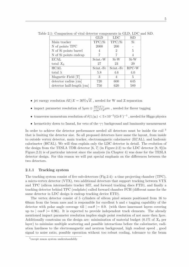
Table 2.1: Comparison of vital detector components in GLD, LDC and SiD.GLD LDC SiD
Main tracker TPC/Si TPC/Si SiN of points TPC 2000 200 -N of Si points barrel 4 2 5N of Si points endcap 7 7 4ECAL Scint.-W Si-W Si-Wtotal X0 27 23 29HCAL Scint.-Fe Scint.-Fe RPC-Wtotal λ 5.8 4.6 4.0Magnetic Field [T] 3 4 5detector radius [cm] 720 600 645detector half-length [cm] 750 620 589
• jet energy resolution δE/E = 30%√E , needed for W and Z separation
• impact parameter resolution of 5µm⊕ 10GeV/c
p sin3/2 θµm , needed for flavor tagging
• transverse momentum resolution of δ(1/pt) < 5×10⁻⁵(GeV )−1 , needed for Higgs physics
• hermeticity down to 5mrad, for veto of the γγ background and luminosity measurement
In order to achieve the detector performance needed all detectors must be inside the coil 3
that is limiting the detector size. So all proposed detectors have same the layout, from insideto outside vertex detector, main tracker, electromagnetic calorimeter (ECAL), and hadroniccalorimeter (HCAL). We will thus explain only the LDC detector in detail. The evolution ofthe design from the TESLA TDR detector [6, 7] (in Figure.2.2) to the LDC detector [8, 9](inFigure.2.3) is of particular interest since the analysis (in Chapter 4) was done for the TESLAdetector design. For this reason we will put special emphasis on the differences between thetwo detectors.
2.1.1 Tracking system
The tracking system consist of five sub-detectors (Fig.2.4): a time projecting chamber (TPC),a micro-vertex detector (VTX), two additional detectors that support tracking between VTXand TPC (silicon intermediate tracker SIT, and forward tracking discs FTD), and finally atracking detector behind TPC (endplate) called forward chamber FCH (different name for thesame detector in LDC design is endcap tracking device ETD).
The vertex detector consist of 5 cylinders of silicon pixel sensors positioned from 16 to60mm from the beam axes and is responsible for excellent b and c tagging capability of thedetector with polar angle coverage till | cos θ |= 0.9. (with three innermost layers coveringup to | cos θ |= 0.96). It is expected to provide independent track elements. The alreadymentioned impact parameter resolution implies single point resolution of not more then 3µm.Additionally constrains on the design are: minimization of material budget (0.1% of X0 perlayer) to minimize multiple scattering and possible interactions before the calorimeter, radi-ation hardness to the electromagnetic and neutron background, high readout speed , goodsignal to noise ratio, possible operation without too robust cooling, tolerance to the beam
3except muon system understandably

6 Chapter 2. International Linear Collider (ILC)
Figure 2.2: Quadrant view of the TESLA detector, dimensions are in mm.
Figure 2.3: Quadrant view of the LDC detector, dimensions are in mm.

7
Figure 2.4: Layout of the tracking system in TESLA TDR detector
Table 2.2: SIT position and sizes in TESLA and LDC detector design.Detector radius [mm] half length in z [mm]TESLA 160 360
300 640LDC 150 180
290 450
induced electromagnetic interference ... The list of the wishes is long as always. Several tech-nologies (DEPFET,CCD) are under consideration hoping that development will bring one ofthem close to the requirements without the significant penalty on any of the issues. Therewere no changes in the detector layout between TESLA and the LDC detector.
SIT detector serves as a bridge between the vertex and the TPC for merging of the tracksegments and provides additional points for low pt tracks that do not reach the TPC. The SITconsist of two layers of silicon strip detectors. Radial positions and lengths of the layers havechanged between TESLA and LDC detector and are summarized in Table.2.2. The designgoal for the point resolution is unchanged and equals 10µm.
The FTD has the same connecting role as the SIT with the addition that it should improveaccuracy of tracking at low angles. Although with the same role as the SIT forward disc areoperation at background conditions that are much closer to the vertex detector thus puttinglarger constrains on the applied technology. It consists of 7 silicon detector discs where thefirst 3 are pixel detector and the remaining 4 are double sided strip detectors. An additionaldisc is proposed in the LDC detector to be in front of the LumiCAL. There were significantreshuffling of the positions and sizes of the FTD discs. Changes are summarized in Table.2.3.
The TPC is main part of the tracking system. The performance goals for the TPC are amomentum resolution of δ(1/pt) ∼ ×10−4(GeV )−1 and dE/dx measurement better then 5%.The main advantage of the TPC, with respect to silicon, is that tracks are measured with largenumber of space point that will provide the highly efficient tracking needed. The measurementis realized with minimal additional material since it will operate at atmospheric pressure withsignificant amount of additional material only in the endplate region. The relatively moderatesingle point precision of 100µ in r − φ and 2mm in z is more then compensated with theability to localize interactions and decays within its volume and provide dE/dx measurement

8 Chapter 2. International Linear Collider (ILC)
Table 2.3: FTD disks layout. Comparison for TESLA and LDC detector (numbers in brack-ets).
inner radius [mm] z position[mm] min angle [o]disc 1 29(40) 200(180) 8.25(12.0)disc 2 32(47.5) 320(300) 5.71(9.0)disc 3 35(57.5) 440(450) 4.55(11.6)disc 4 51(87.5) 550(800) 5.30(10.9)disc 5 72(122.5) 800(1200) 5.14(5.83)disc 6 93(157.5) 1050(1550) 5.06(5.8)disc 7 113(187.5) 1300(1900) 4.96(5.6)
Table 2.4: TPC dimensions in TESLA and LDC detector design.Detector inner r [mm] outer r [mm] TPC Lz/2 [mm] Endplate Lz/2[mm]TESLA 320 1700 2730 230LDC 300 1580 2160 160
to support particle identification. Special attention is needed for the choice of the gas. It shouldgive sufficiently large primary ionization, have small transverse diffusion and fast drift > 5 ∼cm/µs. In addition it should have as small as possible crossection for interaction with thermalneutron background. Signal amplification is realized with Gas Electron Multipliers (GEM)[12]or Micromegas[13] that are able to provide the needed amplification with minimizing ion back-drift at the same time. One of the essentials for application of TPC is not only strength ofthe magnetic field but also its uniformity. The homogeneity condition can be expressed asintegral of radial field component Bφ divided by the longitudinal component Bz over the driftlength. ∫
driftBφ/Bzdz < 2mm (2.1)
The overall size (thus angular coverage) and the total material budget are of special interest forreconstruction. The inner radius is limited with design of the forward region and backgroundconditions. The outer radius is, driven by the needed number of measurement points witha given resolution and in addition is limited by the coil radius and the space requirementsfor the calorimeters. There was a significant size change from the initial design as shown inTable.2.4. Note that the length of active volume has changed by 0.5m! The endplate thicknesshas changed the physical length by keeping the material budget in radiation lengths the same(0.3X0).
The FCH (ETD) has the role of supporting the TPC in the low angle region and to allowaccurate extrapolation into the calorimeter. Except of the name this detector has suffereda technology change from strow tubes to silicon planes. This leeds to the reduction in sub-detector thickness from 70 to 20mm and to a smaller material budget. Even with this changesthe fate of the sub-detector depends on what considerations will prevail between the mini-mization of material in front of the calorimeter or advantage of two precise points after theendplate. The overall tracking system performance goal is δ(1/pt) < 5 × 10⁻⁵(GeV )−1 butthis number, although impressive, is reached only in the high energy limit and for the majorityof physics processes irrelevant since it is driven mostly by Higgs mass measurement. Whatcounts is tracking system reconstruction efficiency over polar angle and energy. Unfortunately
9
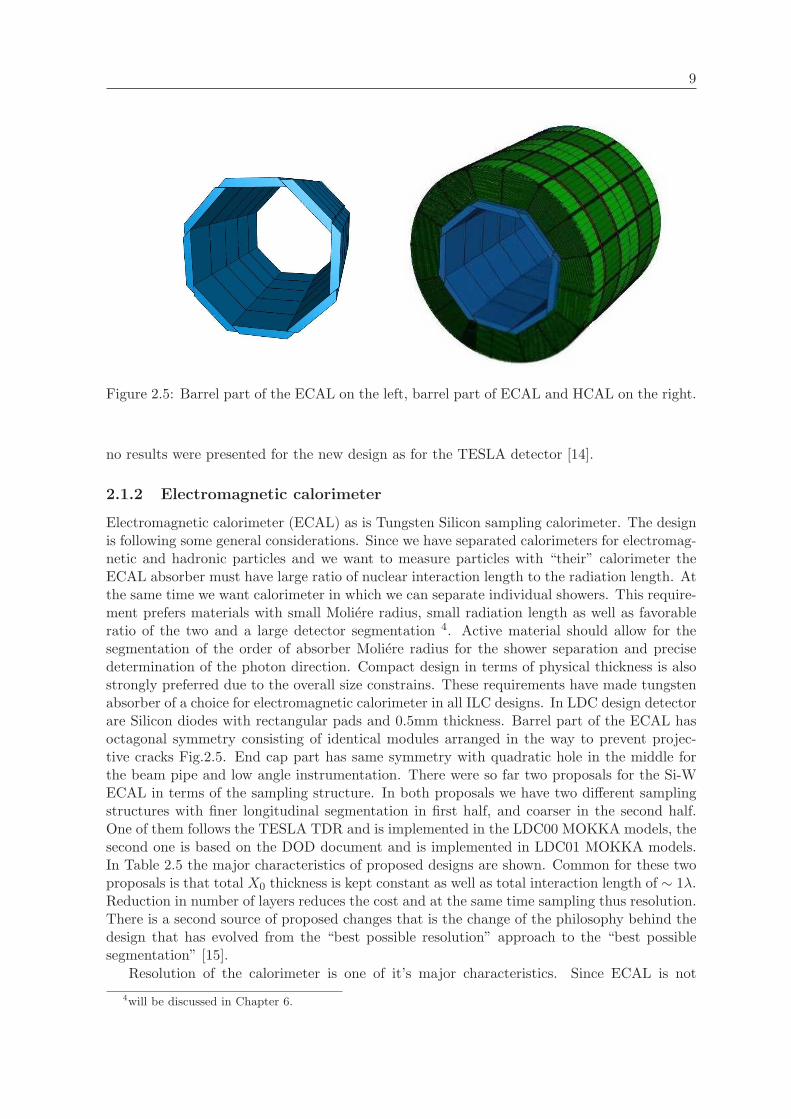
Figure 2.5: Barrel part of the ECAL on the left, barrel part of ECAL and HCAL on the right.
no results were presented for the new design as for the TESLA detector [14].
2.1.2 Electromagnetic calorimeter
Electromagnetic calorimeter (ECAL) as is Tungsten Silicon sampling calorimeter. The designis following some general considerations. Since we have separated calorimeters for electromag-netic and hadronic particles and we want to measure particles with “their” calorimeter theECAL absorber must have large ratio of nuclear interaction length to the radiation length. Atthe same time we want calorimeter in which we can separate individual showers. This require-ment prefers materials with small Moliere radius, small radiation length as well as favorableratio of the two and a large detector segmentation 4. Active material should allow for thesegmentation of the order of absorber Moliere radius for the shower separation and precisedetermination of the photon direction. Compact design in terms of physical thickness is alsostrongly preferred due to the overall size constrains. These requirements have made tungstenabsorber of a choice for electromagnetic calorimeter in all ILC designs. In LDC design detectorare Silicon diodes with rectangular pads and 0.5mm thickness. Barrel part of the ECAL hasoctagonal symmetry consisting of identical modules arranged in the way to prevent projec-tive cracks Fig.2.5. End cap part has same symmetry with quadratic hole in the middle forthe beam pipe and low angle instrumentation. There were so far two proposals for the Si-WECAL in terms of the sampling structure. In both proposals we have two different samplingstructures with finer longitudinal segmentation in first half, and coarser in the second half.One of them follows the TESLA TDR and is implemented in the LDC00 MOKKA models, thesecond one is based on the DOD document and is implemented in LDC01 MOKKA models.In Table 2.5 the major characteristics of proposed designs are shown. Common for these twoproposals is that total X0 thickness is kept constant as well as total interaction length of ∼ 1λ.Reduction in number of layers reduces the cost and at the same time sampling thus resolution.There is a second source of proposed changes that is the change of the philosophy behind thedesign that has evolved from the “best possible resolution” approach to the “best possiblesegmentation” [15].
Resolution of the calorimeter is one of it’s major characteristics. Since ECAL is not
4will be discussed in Chapter 6.

10 Chapter 2. International Linear Collider (ILC)
Table 2.5: Comparison of existing ECAL designs.Detector Number of layers W [mm]([X0]) cell size [mm×mm] total absorber [X0]LDC00 30 1.4 (0.4) 10× 10
10 4.2 (1.2) 10× 10 24LDC01 20 2.1 (0.6) 5× 5
10 4.2 (1.2) 5× 5 24
monolith sub-detector but effectively consisting of two, or even three if one takes into theaccount ECALs tail catcher HCAL, energy dependence of the resolution will not be strictlyin the form as in formulas 2.2 and 2.3 but very close to it. Resolution goal from the TESLATDR calorimeter was5
δE
E=
0.10√E⊕ 0.01 (2.2)
and for LDC version isδE
E=
0.144√E
⊕ 0.005 (2.3)
Large longitudinal segmentation is mainly to reach the desired resolution. Transversal segmen-tation is driven by pattern recognition and separation constrains on the design have becomemore dominant that has reflected itself in to change of the baseline cell size from 10mm to5mm together with more compact design of the calorimeter.
2.1.3 Hadronic calorimeter
Hadronic calorimeter is Iron Scintillator sampling calorimeter. It follows same considerationsabout segmentations as for the ECAL since it should be able to resolve close by hadronicshowers as well as their subcomponents. Layers thickness is 26.5mm and it consists of 20mmof stainless steel and 5mm scintillator, making the longitudinal sampling 1.15 in X0 and 0.12in λ. Resolution goal for the TESLA calorimeter was
δE
E=
0.50√E⊕ 0.01 (2.4)
Granularity is 3 by 3cm through, and taking into account thickness of the absorber and thescintillator leading to almost cubic cell that is very convenient. Granularity was optimized fromthe point of the hadronic shower separation and possible detection of all of it’s subcomponents.Segmentation is considerably smaller then the hadronic shower size as noticed in the [8] , butof the order of Moliere radius ( ≈ 23mm see Table.6.3) as it should be if one would like toresolve subcomponents of hadronic shower and thus not over segmented as one could conclude.Starting layers of HCAL serve also as a tail catcher for the ECAL, with electromagneticresolution of around 20% it is doing excellent task. Only noticeable disadvantage of the currentdesign is it’s small thickness in interaction lengths (only 4.6λ) that could produce significantenergy leakage and degrade reconstruction performance (if you still remember (Table.2.1)thickness of the GLD HCAL is 5.8λ).
5If we accept that detector is that what is implemented in simulation, resolution for the same calorimeterin G4 simulation is 12.5%
11
42503000
300
250
2800
3 m 4 m 5 m
80
Val
ve
82.0 mrad
26.2 mrad
3.9 mrad
82.0 mrad82.0 mrad82.0 mrad82.0 mrad 250280
80
12
92.0 mrad
LumCal
BeamCal
BeamCal 3650...3850
Pump 3350..3500
LumCal 3050...3250
L* 4050
long. distances
EC
AL
EC
AL
HCAL
HCAL
Pole Tip
Pole Tip
QUAD
QUAD
VTX−Elec
VTX−Elec
ElecElec
ElecElecLumCal
LumCal
BeamCal
BeamCal
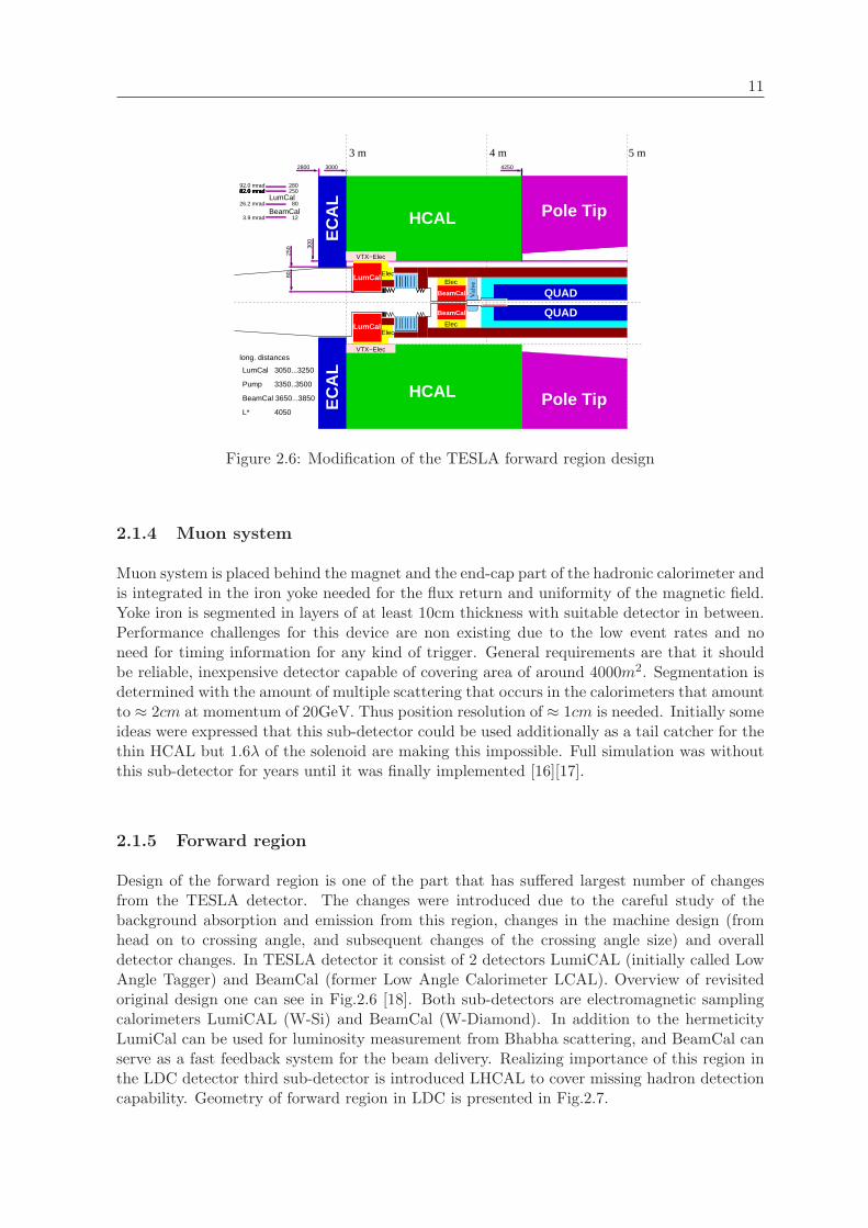
Figure 2.6: Modification of the TESLA forward region design
2.1.4 Muon system
Muon system is placed behind the magnet and the end-cap part of the hadronic calorimeter andis integrated in the iron yoke needed for the flux return and uniformity of the magnetic field.Yoke iron is segmented in layers of at least 10cm thickness with suitable detector in between.Performance challenges for this device are non existing due to the low event rates and noneed for timing information for any kind of trigger. General requirements are that it shouldbe reliable, inexpensive detector capable of covering area of around 4000m2. Segmentation isdetermined with the amount of multiple scattering that occurs in the calorimeters that amountto ≈ 2cm at momentum of 20GeV. Thus position resolution of ≈ 1cm is needed. Initially someideas were expressed that this sub-detector could be used additionally as a tail catcher for thethin HCAL but 1.6λ of the solenoid are making this impossible. Full simulation was withoutthis sub-detector for years until it was finally implemented [16][17].
2.1.5 Forward region
Design of the forward region is one of the part that has suffered largest number of changesfrom the TESLA detector. The changes were introduced due to the careful study of thebackground absorption and emission from this region, changes in the machine design (fromhead on to crossing angle, and subsequent changes of the crossing angle size) and overalldetector changes. In TESLA detector it consist of 2 detectors LumiCAL (initially called LowAngle Tagger) and BeamCal (former Low Angle Calorimeter LCAL). Overview of revisitedoriginal design one can see in Fig.2.6 [18]. Both sub-detectors are electromagnetic samplingcalorimeters LumiCAL (W-Si) and BeamCal (W-Diamond). In addition to the hermeticityLumiCal can be used for luminosity measurement from Bhabha scattering, and BeamCal canserve as a fast feedback system for the beam delivery. Realizing importance of this region inthe LDC detector third sub-detector is introduced LHCAL to cover missing hadron detectioncapability. Geometry of forward region in LDC is presented in Fig.2.7.

12 Chapter 2. International Linear Collider (ILC)
Figure 2.7: LDC design of the forward region
Table 2.6: Design changes between TESLA TDR and LDC DOD detector.Sub-detector TESLA detector LDC detector rating
Tracking volume 1600x2160mm 1700x2750mm negativeTPC inner radius 320mm 300mm positiveEndplate thickness 230mm 160mm positive
ETD thickness 70mm 20mm positiveForward region no hadr. cal. added LHCAL positiveECAL sampling 10+30 layers 10+20 layers negative
resolution 10% 14% negativecell size 10x10mm 5x5 mm positive
HCAL cell size changing through det. uniform 3x3cm positivematerial change stainless steel iron in end-cap negative
2.1.6 Detector design evolution
Five years has passed between TESLA TDR and LDC DOD document. At the moment theseare two significantly different detectors. Some of the sub-detectors have changed some ofthem are still identical (Vertex and muon system). Here I will try to summarize these changes(Table.2.6) and make personal rating of each of them. Beautifully light motive for this can be:“The idea was that some reshuffling of the detector could help making it easier tobuild, cheaper without sacrificing anything important in terms of performance”[19].
Overall size of the detector has changed, detector has shrunk. This is done by reducing thelength of the coil and removing the plug (ferromagnetic transition region between the HCALand YOKE in the end cap needed for flux return). What are the consequences? Angularcoverage of TPC has changed from 7.29 degrees6 in the TDR design to 8.53 in the currentone. Tiny reduction of the inner radius of the TPC cannot compensate drastic reduction in
6endpoint in senstive volume

13
length. In addition to this there was significant redesign in the SIT and FTD layout. SIT isnot covering same angular region till 25 degrees as the vertex detector but till 31.9. Also thelowest angles that are covered by the FTD discs were significantly raised (Table2.3) mostlyby background consideration and in order to relax constrains on the hardware. But takinginto account vertex coverage till 12 degrees and that closest FTD discs coverage till 9 degreestogether with increased distance of of the discs with low angle coverage further from IP onewould expect no tracking for low energy particles below 9 degrees and questionable one forothers below this angle. Radial size reduction will not affect tracking performance significantly.ECAL has also suffered changes number of layers is reduced from 40 to 30, thus sampling iscoarser and resolution has changed accordingly. The hope is that more dense calorimeter andfiner transversal segmentation will compensate for worser resolution by allowing to reduceamount of errors made by reconstruction . On the other hand keeping the same magneticfield and bringing the calorimeter face closer to the IP means that average distance betweenthe particles on the face of the calorimeter will also decrease reducing part of the promisedgain (if any). Since the plug is removed in order to fulfill requirements of field homogeneityneeded for the tracking (eq.2.1 ) HCAL now needs to be changed also. Absorber in the endcap part must be ferromagnetic. This will increase amount of dead material in HCAL sincesupport should now cope not only with calorimeters own weight but also with magnetic forces.Additionally corner part of the HCAL end-cap is now close to the edge of the coil thus in theregion of highly inhomogeneous field that will add complications to the calibration7.
Angular coverage of the the tracking system is reduced roughly by 2 degrees, resolutionof the ECAL is reduced with unclear gain in reconstruction performance, amount of deadmaterial in the HCAL is increased but the detector is cheaper,easier to build and we have notsacrificed anything important. By the way if one looks at Reference Design Report [20] LDCis still only detector that has single sub-detector more expensive then the coil. Why is notpossible to accept that superior detector has its price is beyond my ability to comprehend.
What was the intention of such accelerator and detector introduction? First of all to makeit clear that scope of the project is changing together with the detector designs, and thatthings that are assumed realistic and for granted at one point in time may look different atanother. Second, altho people tend to mix TESLA and LDC detector these are two differentdetectors and should be treated as such.
7to be discussed in Chapter 5


Chapter 3
Quartic couplings
Unfortunately before we can jump to the measurement of quartic couplings and interpretationof the result we need a bit longer theoretical introduction in order to make the text readableto non-expert. We will start from the Standard Model (SM) as a basic theory of elementaryparticles and their interactions as we know them today, explain how the electroweak sector isrealized within SM and what is the solution to the mass generation within the SM. After thatEffective Lagrangian will be introduced as a general framework within which we will discussquartic couplings. At the end we will introduce relations between the possible new resonancesand quartic couplings. Together with the proposed approach to the measurement of quarticcouplings this will provide us with the understanding needed for the next chapter. If someonedoes not like my stile or amount of detail dedicated to particular issue you can find in books[21],[21] and reviews and lectures [23], [24],[25] additional quotations will be within the text onthe specific issues. There is absolutely no personal contribution to the content of this chapterexcept the errors in typing. Basic notation is explained in appendix A.
3.1 Standard Model
Standard Model [26] is a re-normalizable quantum field theory that describes electroweak andstrong interactions of quarks and leptons which are the most elementary components of matterknown at present. One of the essential features of the model is that both the electroweak andthe strong force are introduced as gauge interactions. In this description it is possible to definethree separate parts: First the matter sector which is made of fermionic fields; second thereare vector boson gauge fields and finally the symmetry breaking sector. This sector is neededin order to provide masses for fermions and weak bosons. Simplest realization of the symmetrybreaking sector is a doublet of self interacting scalar fields - famous Higgs boson. The matterpart of the SM consist of fermions organized in three generations as shown in Table.3.1. Eachgeneration is made of two quark flavors (u and d like) and two leptons (neutrino and electronlike). All these particles are accompanied by their corresponding anti particles with same massand opposite charges.
In the SM there are two types of gauge interactions. Strong interaction among the quarksmodeled by the quantum chromo dynamics - gauge theory based on the SU(3) symmetrygroup. Electroweak theory describes the electromagnetic and weak interaction on the basis ofSU(2)L × U(1)Y group. Particles are arranged in the multiplets that transform according tothe symmetry of interaction.
Neutrinos occur only in the left-handed (negative helicity ) state and anti neutrinos onlyin the right-handed state. This implies that only ψL and ψ†L can be present in the field theory
15

16 Chapter 3. Quartic couplings
Table 3.1: Elementary particles and their interactions.Quarks Leptons
first generation u d νe esecond generation c s νµ µ
third generation t b ντ τ
strong interaction yes yes no nostrong interaction color triplet color singlet
electromagnetic int. yes yes no yeselectromagnetic int. Q = 2/3 Q = −1/3 Q = 0 Q = −1
weak interaction yes yes yes yes
for the neutrinos. Theory can be formulated with two spinor(
10
)and
(01
).
We could introduce the theory in at least two ways formal, mathematical one and morehistorical. Second approach is more useful to demonstrate how the theory was developed andsubsequently patched, and updated to accommodate experimental facts.
Fermi theory
After Pauli [30, 31] introduced neutrino to explain continuous spectrum of β decay , Fermi[32] proposed field theory for β decay, assuming existence of neutrino. In analogy to ”thetheory of radiation that describes the emission of a quantum of light from an excited atom”Fermi proposed a current-current Lagrangian to describe β decay.
L =GF√
2(ψpγµψn)(ψeγµψν) (3.1)
This is effectively start of the electroweak theory. Gammov and Teller [33] proposed anextension to Fermi theory to describe also transitions wit ∆J 6= 0. Pontecorvo [34] first ideaabout universality of weak interactions i.e. decay and capture have same origin. Thus ingeneral
Mfi ≈∑
i
Ci(upOiun)(ueOiuν) (3.2)
where the sum is over the possible form of the bilinear covariants i=S,V,T,A,P .
S = 1, P = γ5, V = γµ, A = γµγ5, T = σµν (3.3)
Nuclear transition with ∆J = 0 are described by the interaction of SS and/or VV type,while ∆J = 0,±1 can be take into account by AA and or TT interactions ( P → 0 in non-relativistic limit). Interference between them are proportional to me/Ee an should increasethe emission of low energy electrons. Since this is not observed the weak Lagrangian shouldcontain SS or V V and AA or TT terms. From four possible combinations ST,SA,VT andVA two ( SA and VT could be discarded on the basis of energy spectrum). In order toaccommodate parity-violating effects one must add terms to the matrix elements which arepseudo-scalars, obtained by contracting two covariants which have the opposite behavior underparity transformation. Most general pseudo-scalar is thus
Mfi ≈∑
i
C ′i(upOiun)(ueOiγ5uν) (3.4)

17
with different coefficients C ′i for parity-violating terms. From experiment beta decay is timereversal invariant thus the coefficients Ci and C ′i must be real. Neutrino and antineutrino havedefinite handedness -parity violation is maximal - and this implies C ′i = ±Ci
Mfi =G√2
∑
i
Ci(upOiun)(ueOi(1± γ5)uν) (3.5)
Precise measurement of energy spectrum, and angular correlations lead to determination ofV-A nature for beta decay. Problem of the Fermi theory was energy behavior of scatteringprocesses. Point like neutrino electron scattering cross section (ignoring the spin effects) is:
σ(νee→ νee) =G2s
π(3.6)
On the other hand maximum elastic cross section allowed by unitarity for point like or S wavescattering is:
σmaxel =4πk2
(2l + 1) =4πk2
(3.7)
And now we have clear contradiction of eq.3.6 and eq.3.7, that allows to estimate energy atwhich the theory breaches unitarity that is around 300GeV. This implied that Fermi theory,could not be final theory for the weak interactions but, is effective low energy theory.
Gauge principle
There are in general two types of symmetries global (space time independent) and local (func-tions of space and time coordinate). Let us now try other way around we will ask for thetheory to be invariant under local transformation and look what interaction it implies. Bestexample for this is the Quantum Electrodynamics (QED) that has become a prototype ofquantum field theory. Thus we will start from the Dirac free Lagrangian
Lψ = ψ(iγµ∂µ −m)ψ (3.8)
and investigate its behavior under global and local transformations. It is obvious that A.26 isinvariant under transformation
ψ → ψ′ = exp[−iα]ψ (3.9)
were α is scalar constant (space-time independent). Under local transformation
ψ → ψ′ = exp[−iα(x)]ψ (3.10)
The phase transformation is local one dimensional transformation that additionally satisfiesthe unitarity condition i.e. it is a representation of the U(1) group. Lagrangian transforms to
L → L′ = L+ ψγµψ(∂µα) (3.11)
and is not invariant. However if we introduce the gauge field Aµ through the minimal coupling
∂µ → Dµ ≡ ∂µ + ieAµ (3.12)
and at the same time require that Aµ transforms as
Aµ → A′µ = Aµ +1e∂µα. (3.13)

18 Chapter 3. Quartic couplings
we getL → L′ = L − eψγµψA
µ (3.14)
Thus invariance is kept under simultaneous transformations 3.10 and 3.13 and replacement∂µ → Dµ that together form a gauge transformation. Important to mention is that derivativesof the field are transforming in the same way as the field itself making any Lagrangian thatconsist of fields and their derivatives manifestly invariant.
D′µψ
′ = exp[−iα(x)]Dµψ (3.15)
Thus coupling between the matter field and the gauge field arrises naturally when we requirethe invariance under local gauge transformation of the kinetic energy terms in free fermionLagrangian. Since the electromagnetic strength tensor is invariant under the gauge transfor-mation
Fµν ≡ ∂µAν − ∂νAµ (3.16)
so is the Lagrangian for the free gauge field.
LA = −14FµνF
µν (3.17)
making together with 3.14 Lagrangian of the QED.
L = Lψ − eψγµψAµ − 1
4FµνF
µν (3.18)
Direct mass term −1/2 m2AµAµ violates gauge invariance thus gauge boson is massless, and
one needs another mechanism if one would like to have massive gauge boson field. Since thetransformation is commutative QED is an example of Abelian gauge theory.
Yang-Mills theories
As suggested by Heisenberg [35] in 1932 under nuclear transitions proton and neutron canbe regarded as degenerated since their masses are similar and electromagnetic interaction isnegligible. Therefore arbitrary combination of their wave functions would be
ψ ≡(ψpψn
)(3.19)
Lagrangian should be invariant under matter field transformation
ψ → ψ′ = Uψ (3.20)
where U is unitary transformation (U †U = UU † = 1) to preserve normalization. If det|U | = 1, U represents Lie group [53] SU(2)
U ≡ exp[−iτa
2αa(x)] ' 1− i
τa
2αa(x) (3.21)
where τa, a=1,2,3 are Pauli matrices. Important difference to the example of QED is thatgenerators of SU(2) do not commute giving the name to the theories as non Abelian. Resultwas generalized by Utiyama [36] for any non-Abelian group satisfying Lie algebra. Lagrangianshould be invariant under matter filed transformation 3.20 with
U ≡ exp[−iT aαa(x)] (3.22)

19
where T a is convenient representation of the generators ta. Introducing one gauge field foreach generator and defining the covariant derivative by
Dµ ≡ ∂µ − igT aAaµ (3.23)
this assures the invariance under local non-Abelian gauge transformation for the termscontaining the fields and its gradients as long as the gauge field transformation is
T aAaµ → U(T aAaµ +
i
g∂µ)U−1 (3.24)
or in infinitesimal form i.e for U ' 1− iT aαa(x)
Aa′µ = Aaµ −
1g∂µα
a + CabcαbµA
cν (3.25)
Generalized form of he strength tensor for a non Abelian Lie group
F aµν ≡ ∂µAaν − ∂νA
aµ + gCabcA
bµA
cν (3.26)
were Cabc is structure constant of the group (sec.A.0.5, eq.A.14). However a direct mass termfor the gauge bosons is again not invariant:
AaµAaµ →
(Aaµ −
1g∂µα
a + CabcαbAcµ
)(Aaµ − 1
g∂µα
a + CadeαdAeµ
)(3.27)
Form of the strength tensor 3.26 produces important feature of non-Abelian theory, since
F ∝ (∂A− ∂A) + gAA (3.28)
gauge part of the Lagrangian is:
L ∝ (∂A− ∂A)2 + g(∂A− ∂A)AA+ g2AAAA (3.29)
thus we now have additional self interaction of the gauge fields,where second term describestriple and third quartic couplings. Triple and quartic couplings arise naturally in non-Abeliangauge theory.
3.1.1 Electroweak sector
From the introduction of the Fermi theory to late 50-ties large amount of experimental factsabout weak interactions were collected that allowed attempts to construct a gauge theory.Lepton number conservation ( pion decay π+ → µ+νµ and consequent reaction νµ+n→ p+µ−
but no νµ + n → p + e−). Also no muon decay channels of the kind µ± → e± + γ orµ± → e± + e+ + e− i.e. no flavor-changing neutral currents. Confirmation of parity violationin weak processes by Wu et al. [47] in 1957. Measurement of the neutrino helicity [48] in 1958,and decay chain of pions π+ → µ+νµ, µ
+ → e+ + νe + νµ [49] in 1957. Antineutrino helicitymeasured in decay of polarized neutrons [50] in 1958.
Several attempts to construct a gauge theory of weak interactions. In 1957, Schwinger[37] suggested a model based on the group O(3) with triplet gauge fields (V +, V −, V 0) ,were charged gauge bosons were associated to weak bosons and the neutral was identified asphoton. This was before the V-A structure of the weak current was established [38, 39, 40].First attempts to incorporate V-A structure in gauge theory was made by Bludman [41] andLopes [42] in 1958. Gashow [43] in 1961 , and Salam and Ward [26] in 1964 proposed a model

20 Chapter 3. Quartic couplings
based on SU(2) ⊗ U(1) group,where U(1) i associated to the leptonic hypercharge (Y) thatis related to the weak isospin (T) through the Gell-Mann-Nishijima formula Q = T3 + Y/2.Theory required four gauge bosons a triplet associated to SU(2) generators an a neural fieldrelated to U(1). Mass terms were put by hand ! Weinberg [44], Salam [45] employed the ideaof spontaneous symmetry breaking and the Higgs mechanism to give mass to the weak bosonsand preserve gauge invariance. Renormalizability of the theory was finally proven by ’t Hooft[46] We require local gauge invariance under both SU(2)L and independently U(1)Y this willintroduce interactions inthe free-field Lagrangian. In order to incorporate experimental factfermions are organized in left handed doublets and right handed singlets.
L =(νll−
)
L
, R = l−R (3.30)
where l = e, µ, τ . Theory does not necessarily involve right-handed neutrinos, and their inclu-sion in spectrum is allowed but not required. We start as usual from free fermion Lagrangian:
L = Liγ5∂L+ Riγ5∂R (3.31)
Under local gauge transformations the fermion fields transform as below:
SU(2)L U(1)YL→ exp[−i(g/2)~Λ(x)~τ ]L L→ exp[−i(g′/2)λ(x)Y ]LR→ R R→ exp[−i(g′/2)λ(x)Y ]R
(3.32)
where λ(x), ~Λ(x) are arbitrary coordinate functions, τ are Pauli matrices (eq.A.9). Since wehave now introduced transformation we can construct the covariance derivative
Dµ = ∂µ +12ig~τ ~Wµ+
12ig′Y Bµ (3.33)
i.e. for left handed doublets
DLµ = ∂µ +12ig~τ ~Wµ+
12ig′YLBµ (3.34)
and for right handed singlets
DRµ = ∂µ +12ig′YRBµ (3.35)
and defining the strength tensor for the gauge fields
W iµν ≡ ∂µW
iν − ∂νW
iµ + gεijkW j
µWkν
Bµν ≡ ∂µBν − ∂νBµ (3.36)
we can write the free Lagrangian for the gauge fields.
Lgauge = −14W iµνW
i µν − 14BµνB
µν (3.37)
Now we can look at the fermion boson part of the Lagrangian, again replacing the covariantderivatives in the free Lagrangian.
L′ → L+ Liγµ(ig
2τ iW i
µ + ig′
2Y Bµ)L+ Riγµi
g′
2BµR (3.38)

21
and separate the “charged” part of the Lagrangian:
−gLγµ(τ1
2W 1µ +
τ2
2W 2µ)L (3.39)
and compare it with the charged current leads to the definition of the physical charged gaugebosons.
W± =1√2
(W 1µ ∓ iW 2
µ
)(3.40)
Sorting the terms in the “neutral” part of eq.3.38 we get:
−g2Lγµτ3LW 2
µ −g′
2(LγµY L+ RγµY R)Bµ
= −g2(νLγµ − lLγ
µlL)W 3µ +
g′
2(νLγµ + lLγ
µlL + 2lRγµlR)Bµ (3.41)
that we want to assaign to a neutral current, this can be acheaved by rotation of the neutralfields to new fields A and Z
Aµ = Bµ cos θW +W 3µ sin θW
Zµ = −Bµ cos θW +W 3µ sin θW (3.42)
where the weak mixing angle θW (called Weinberg angle) is define as tan θW = g′/g , and elec-tromagnetic coupling constant is then e = g sin θW = g′ cos θW . Now we have full descriptionof matter and fields part of theory. Note that all the particles are still massless. Introductionof mass terms by hand breaks down the gauge invariance. Since it was know that particleshave masses long before development of theory meaningful explanation must exist.
3.1.2 Symmetry breaking sector
For incorporating the masses in the electroweak theory there were two essential additionalingredients needed first is Goldston theorem [28, 29] stating that whenever exact continuousglobal symmetry is spontaneously broken, i.e. it is not the symmetry of physical vacuum, thetheory contains one massless scalar particle for each broken generator of original symmetrygroup. This seams not to help since it can only generate massless particles and we alreadyhave too much of them. Symmetry requirements came to the rescue again. If we require thatthe Lagrangian which exhibits spontaneous symmetry breaking is also invariant under local,rather then global transformation we get the Higgs mechanism [56, 57, 58]. We will considerspontaneous breaking of a local gauge symmetry, namely SU(2)L × U(1)Y . We introduce ascalar doublet of complex fields:
φ =(φ+
φ0
)=
1√2
(φ1 + iφ2
φ3 + iφ4
)(3.43)
and its LagrangianL = (∂µφ)†(∂µφ)− µ2φ†φ− λ(φ†φ)2 (3.44)
The Lagrangian is manifestly invariant under global SU(2) transformations. In order to makeit locally invariant we replace.
Dµ = ∂µ + igτi2W iµ + ig′
Y
2Bµ (3.45)

22 Chapter 3. Quartic couplings
and the gauge invariant Lagrangian is
L =(Dµφ
)†(Dµφ
)− V (φ)− 1
4~Wµν
~Wµν − 14BµνB
µν (3.46)
minimum of the potential part is at
φ†φ =12(φ2
1 + φ22 + φ2
3 + φ24) = −µ
2
2λ=v2
2(3.47)
an by making a specific choice for the minimum i.e. breaking the symmetry
φ1 = φ2 = φ4 = 0 φ23 = v2 (3.48)
now we expand around chosen ground state of the vacuum.
φ(x) =1√2
(0
v +H(x)
)(3.49)
thus arbitrary filed can be parameterized in the form
φ(x) =1√2
(0
v +H(x)
)exp
[ i~α(x)~τ2v
](3.50)
takin into account gauge transformation of the field
φ(x) → φ′(x) = φ(x) exp[ i~Λ(x)~τ
2]
(3.51)
we can choose a gauge parameter to cancel exponential terms so that
φ′(x) =1√2
(0
v +H(x)
)(3.52)
Since only one component gets the vacuum expectation value the SU(2) symmetry isbrocken, with hypercharge Y 6= 0 also U(1) is broken. Although choice of the vacuum mayseem arbitrary it is not. If φ+ would have a vacuum expectation value charge would not beconserved contrary to observations. Vacuum is invariant under φ0 → φ′0 = exp[−i(x)Q]φ0 =φ0 that is a U(1) transformation of electromagnetism thus we say that SU(2)L × U(1)Y isbroken to U(1)em. taking together eq.3.46 and eq.3.49 and expanding, usual mass termsappear with:
MW =12gv,MZ =
12
√g2 + g′2 and Mγ = 0 (3.53)
As for the bosons, direct mass terms are breaking gauge invariance for the fermions:
−mee = −me(PL + PR)e = −m(eReL + eLeR) (3.54)
Adding the gauge invariant part to the Lagrangian
L = −ge[LφeR + eRφL] (3.55)
substituting L and φ we get
L =−gev√
2(eReL + eLeR)− ge√
2(eReL + eLeR)H (3.56)
23
First term has the from of an electron mass term with mass:
me =gev√
2(3.57)
where ge is the Yukawa coupling. A similar solution is applied for the generation of masses forthe quarks. At this stage we have a theory that incorporates masses of all known particles butthis solution to the mass problem is part of the problem itself. A first objection is an estheticone, we have postulated a field with just the right quantum numbers to patch the theory andwhy should the nature obey this. The Higgs boson is still not observed. Since λ and µ arefree parameters as well as all the Yukawa couplings the predicivity of the theory with respectof the mass spectrum is zero thus leaving no explanation for the observed mass spectrum.A vacuum expectation value of v ∼ 250GeV is incompatible with the present cosmologicalmodels. The Higgs mass is affected by quadratic radiative corrections that would make it ofthe order of the scale of the new physics phenomena. If we want to be in the experimentallyallowed range we have to ask for extremely fine and unnatural cancellation of divergences.The Higgs mass mh = v
√2λ is also a free parameter leaving open questions about weak or
strong nature of symmetry breaking sector.
Anomalous couplings
General form of the Lagrangian for the triple gauge couplings (TGC) sector is:
LTGC = ie[gγ1Aµ(W
−ν W
+µν −W+µ W
−µν) + κγW−µ W
+ν A
µν +λγ
M2W
W−νµ W+
µρAρµ
]
+iecWsW
[gZ1 Zµ(W
−ν W
+µν −W+ν W
−µν)
+κZW−µ W
+ν Z
µν +λZ
M2W
W−νµ W+
νρZρµ
](3.58)
The CP conserving couplings are related to the charge qW , the magnetic dipole momentµW and electric quadrupole moment QeW of the W boson.
qW = egγ1
µW =e
2MW(gγ1 + κγ + λγ)
QeW = − e
M2W
(κγ − λγ) (3.59)
The behavior under charge (C) and parity (P) conjugation can be used to divide them intoseveral groups. Couplings gV1 , κV and λV conserve C and P. Electromagnetic gauge invariancerequires gγ1 = 1 and gγ5 = 0 and reduces overall number of C and P conserving couplings to 5.SU(2) gauge invariance requires
∆κZ = ∆gZ1 −∆κγ tan2 θW
λZ = λγ (3.60)
reducing number of free couplings to three. General form of the Lagrangian covering quartic

24 Chapter 3. Quartic couplings
couplings sector is:
LQGC = e2[gγγ1 AµAνW−µ W
+ν − gγγ2 AµAµW
−νW+ν ]
+e2cWsW
[gγZ1 AµZν(W−µW+ν +W+
µ W−ν)− 2gγZ2 AµZµW
−νW+ν ]
+e2c2Ws2W
[gZZ1 ZµZνW−µ W
+ν − gZZ2 ZµZµW
−νW+ν ]
+e2
2s2W[gWW
1 W−µW+νW−µ W
+ν − gWW
2 (W−µW+µ )2]
+e2
4s2W c4W
hZZ(ZµZµ)2 (3.61)
3.2 Effective Lagrangian
A theory based only on the observed degrees of freedom (without Higgs) is non-renormalizable.At high energies there is a cutoff scale at which this theory stops to be predictive. In the caseof the e+e− → ν+W− in the absence of the Higgs unitarity is violated around ∼ 1.2TeV .Together with objections made to the SM we are almost in the same situation as in the earlydays of the Fermi theory. In this analogy and following historical development one is temptedto make the same conclusion that we are dealing with low energy effective theory and thatone should collect enough experimental facts to conclude about the “true”theory. The wayto do this is using the Effective Lagrangian [54, 55]. The lowest order Lagrangian is invariantunder SU(2)L × SU(2)R that is broken to SU(2)C although SU(2)C is broken by U(1)Y andit is affected by correction to the ρ parameters ( ρ ≈ 1 +O(
g′2))
Wµν = ∂µWν − ∂νWµ + ig[Wµ,Wν ] (3.62)
Bµν = Σ(∂µBν − ∂νBµ
)τ3
2Σ† (3.63)
Where the usual fields are W aµ and Bµ with abbreviation
Wµ = W aµ
τa
2and Bµ = Bµ
τ3
2(3.64)
and additional field Σ with suitable transformation law. The field Σ(x) is 2 × 2 ma-trix which transforms under local SU(2)L transformation U(x) = exp[−iαa(x) τa
2 ] and U(1)Ytransformation V = exp(iβ(x) τ
3
2 ) in the form
Σ(x) → U(x)Σ(x)V †(x) (3.65)
Introducing further abbreviations
Vµ = Σ(DµΣ)† and T = Στ3Σ† (3.66)
where D is a covariant derivative, allows to rewrite the direct mass terms and introduce thepossibility to add an invariant potential term
LΣ = −µ2v2
4tr[Σ†Σ] +
λv4
16tr[Σ†Σ]2 + ... (3.67)

25
Σ = exp(− i
vw
)(3.68)
Goldston bosons w ≡ waτa The Scalars wa are the Goldston bosons associated with sponta-neous symmetry breaking. All together leading to the lowest order chiral Lagrangian:
L0 = −12tr[WµνWµν ]− 1
2tr[BµνBµν ]− v2
4tr[VµVµ] + β′L′0 +
∑
i
αiLi (3.69)
L′0 =v2
4tr[TVµ ] tr[TVµ ] (3.70)
Imposing CP-invariance on the effective Lagrangian the compleat list of dimension-four oper-ators not contained in :
L1 = gg′ tr[ ΣBµνΣ†Wµν ]L2 = ig′ tr
[ΣBµνΣ† [Vµ,Vν ]
]
L3 = ig tr[Wµν [Vµ,Vν ]
]
L4 =(tr[VµVν ]
)2
L5 =(tr[VµVµ ]
)2 (3.71)L6 = tr[VµVν ] tr[TVµ ] tr[TVν ]L7 = tr[VµVµ ] tr[TVν ] tr[TVν ]
L8 =14g2
(tr[TWµν ]
)2
L9 =i
2g tr[TWµν ] tr
[T[Vµ,Vµ ]
]
L10 =12
(tr[TVµ ] tr[TVν ]
)2
And additional restricted set of dimension 6 operators :
Lλ1 = ig3
3M2W
tr(WµνWρ
νWρµ
)
Lλ2 = ig2g′
M2W
tr(BµνWρ
νWρµ
)
Lλ3 = ig2
M2W
tr([
Vµ,Vν]Wρ
νWρµ
)(3.72)
Lλ4 = ig2
M2W
tr([
Vµ,Vν]BρνWρµ
)
Lλ5 = igg′
2M2W
tr(T
[Vµ,Vν
])tr
(TWρ
νWρµ
)
In case of nonlinear symmetry representation the Lagrangian contains terms of arbitraryhigh dimension. At each new order of perturbation new terms are introduced with the dimen-sion of Σ-dependent term increased by two. In the SM quartic couplings sector can be thenwritten:
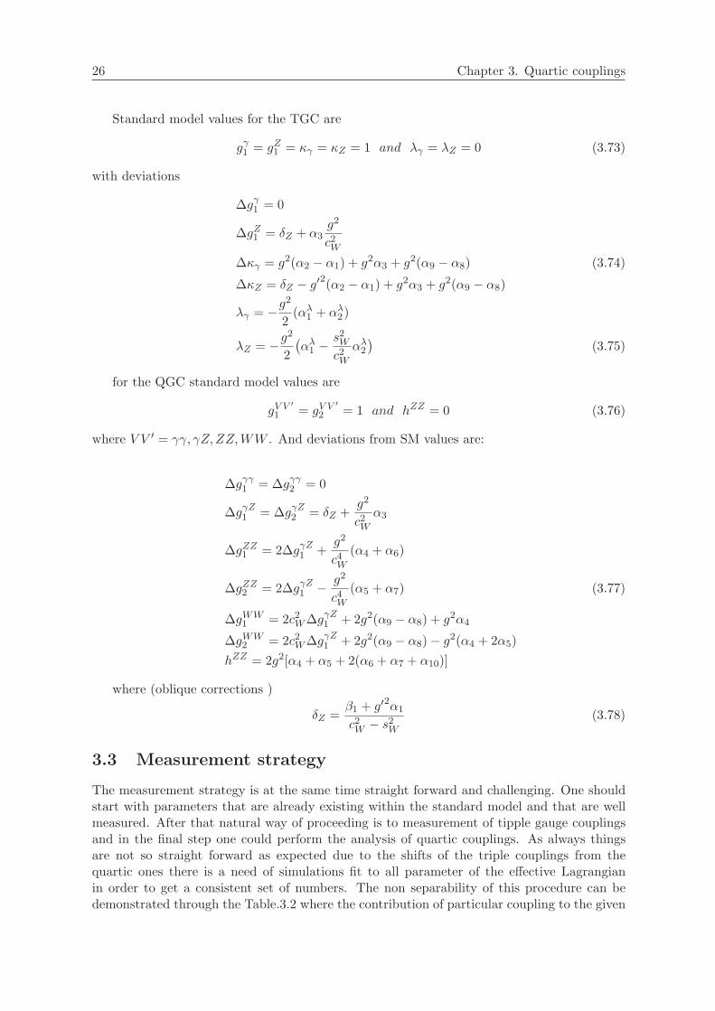
26 Chapter 3. Quartic couplings
Standard model values for the TGC are
gγ1 = gZ1 = κγ = κZ = 1 and λγ = λZ = 0 (3.73)
with deviations
∆gγ1 = 0
∆gZ1 = δZ + α3g2
c2W∆κγ = g2(α2 − α1) + g2α3 + g2(α9 − α8) (3.74)
∆κZ = δZ − g′2(α2 − α1) + g2α3 + g2(α9 − α8)
λγ = −g2
2(αλ1 + αλ2)
λZ = −g2
2(αλ1 −
s2Wc2W
αλ2)
(3.75)
for the QGC standard model values are
gV V′
1 = gV V′
2 = 1 and hZZ = 0 (3.76)
where V V ′ = γγ, γZ, ZZ,WW . And deviations from SM values are:
∆gγγ1 = ∆gγγ2 = 0
∆gγZ1 = ∆gγZ2 = δZ +g2
c2Wα3
∆gZZ1 = 2∆gγZ1 +g2
c4W(α4 + α6)
∆gZZ2 = 2∆gγZ1 − g2
c4W(α5 + α7) (3.77)
∆gWW1 = 2c2W∆gγZ1 + 2g2(α9 − α8) + g2α4
∆gWW2 = 2c2W∆gγZ1 + 2g2(α9 − α8)− g2(α4 + 2α5)
hZZ = 2g2[α4 + α5 + 2(α6 + α7 + α10)]
where (oblique corrections )
δZ =β1 + g′2α1
c2W − s2W(3.78)
3.3 Measurement strategy
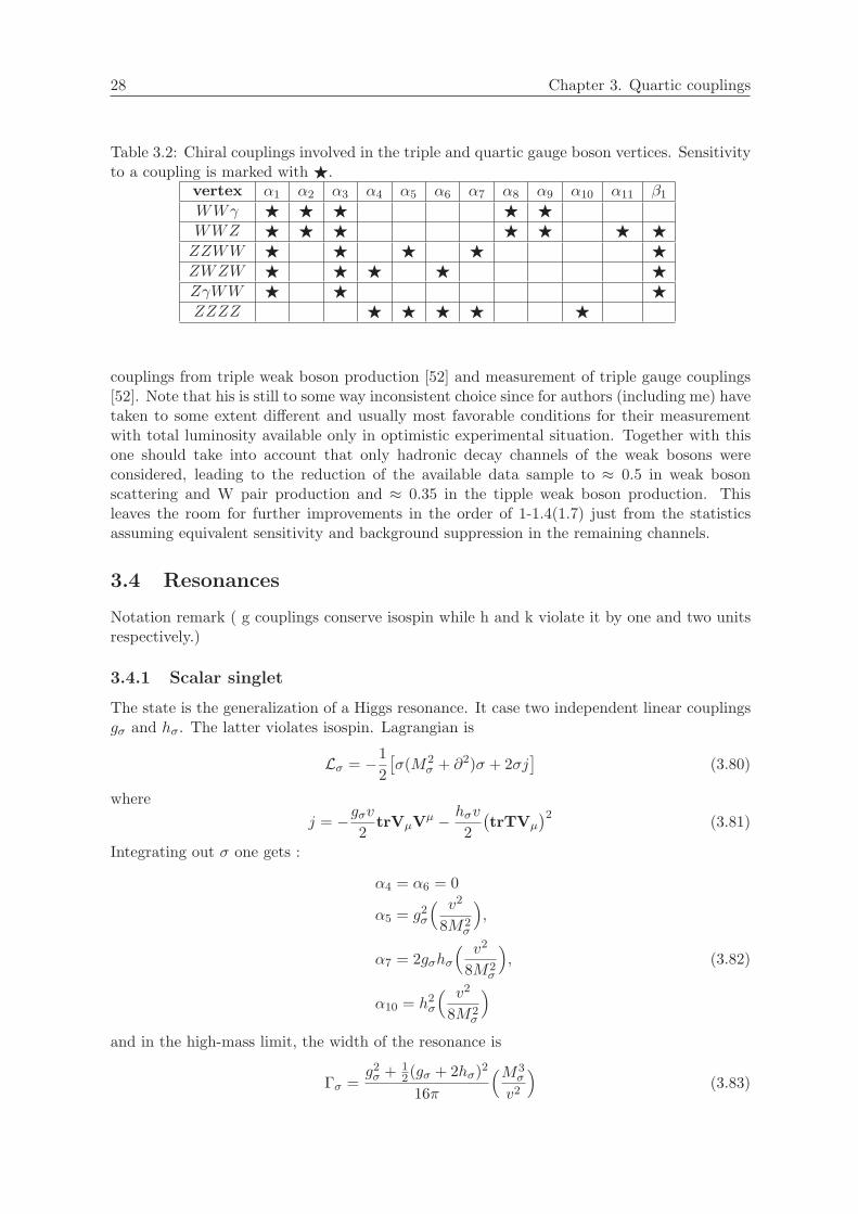
The measurement strategy is at the same time straight forward and challenging. One shouldstart with parameters that are already existing within the standard model and that are wellmeasured. After that natural way of proceeding is to measurement of tipple gauge couplingsand in the final step one could perform the analysis of quartic couplings. As always thingsare not so straight forward as expected due to the shifts of the triple couplings from thequartic ones there is a need of simulations fit to all parameter of the effective Lagrangianin order to get a consistent set of numbers. The non separability of this procedure can bedemonstrated through the Table.3.2 where the contribution of particular coupling to the given
27
vertex is labeled. Vertices WWγ and WWZ are exploited in processes e+e− → W+W− ande+e− → e±νW∓ for measurement of tipple couplings. For the remaining vertices we can seethat there is also contribution of α1 and α3 that contribute the triple gauge couplings. Thusit is essential to know the triple coupling with the precision that will allow correct calculationof the matrix elements for the sensitive processes and in the same time correct extraction ofthe limits to the quartic couplings.
One should cover all the parameters of the chiral Lagrangian. Radiative correction to themasses and couplings of the gauge bosons can be absorbed into tree parameters. The relationsof the S,T,U parameterization and coupling constants of the effective Lagrangian are:
∆S = −16πα1 ∆T = 2β1/αQED ∆U = −16πα8 (3.79)
S,T,U are defined with the SM expectation subtracted so that S=T=U=0 in the SM perdefinition. Values are well constrained by LEP , SLD and Tevatron experiments.
Next set of parameters are α2, α3, α9 that contribute to the trilinear couplings. Measure-ment of this couplings is favorable due to the vertices appearing in the processes of the highestcross section (single W and W and Z pair production) almost without SM background dia-grams, and the coupling can be determined with excellent precision from W-pair produciton.
After that one can proceed to the analysis of the remaining parameters α4, α5, α6, α7, α10.Where first two α4, α5 conserve isospin symmetry , and other three violate. Thus In theanalysis we assumed that the parameters except ones we are interested are determined withprecision well beyond one that will interfere with quartic coupling determination.
Extraction of the quartic coupling based the direct measurement can rely on three
• vector boson scattering - that is favorable due to cross section rising with energy, butthe effective scattering energy is significantly smaller due to the large fraction of energycarried away by e or ν. Disadvantage is also relatively small (∼ fb) cross section thatis requiring large integrated luminosity and excellent detector performance to eliminatebackground and separate channels.
• triple vector boson production- cross section is falling with energy thus making it apreferred process for initial constraining of the coupling at first stage of the ILC (max 500GeV). It also suffers from ∼ fb cross section and fact that only two processese+e− →WWZ,ZZZ contain quartic couplings through the linear combination makingimpossible simultaneous determination of all 5 couplings without additional informationor assumptions.
• rescattering in vector boson pair production- computation of the effects is theoreticallychallenging and unfortunately only J=1 amplitude is accessible.
In order to obtain consistent set of values for the couplings one should not consider men-tioned items as separate measurement. Final word can be sad only after processing all sourcesof information and a combined fit like those done by LEP electroweak group.
After performing the analysis one most general way possible it is of interest to put theresult into framework of possible physics scenario. Since it is expected that we see only “lowenergy” effects of the underling physics Historically interpretation of the reachable sensitivitieswas in the value of the cutoff scale i.e. scale were our picture starts to be predictive and newphenomena sets one. Dangers of such approach and well known [52] and we will see onthe example of this measurement can be significantly off leading to the wrong conclusions.Thus result will be interpreted within possible physics scenario of a to be resonance tryingto demonstrate attempt of the combined fit by incorporating measurements of the quartic
28 Chapter 3. Quartic couplings
Table 3.2: Chiral couplings involved in the triple and quartic gauge boson vertices. Sensitivityto a coupling is marked with F.
vertex α1 α2 α3 α4 α5 α6 α7 α8 α9 α10 α11 β1
WWγ F F F F FWWZ F F F F F F FZZWW F F F F FZWZW F F F F FZγWW F F FZZZZ F F F F F
couplings from triple weak boson production [52] and measurement of triple gauge couplings[52]. Note that his is still to some way inconsistent choice since for authors (including me) havetaken to some extent different and usually most favorable conditions for their measurementwith total luminosity available only in optimistic experimental situation. Together with thisone should take into account that only hadronic decay channels of the weak bosons wereconsidered, leading to the reduction of the available data sample to ≈ 0.5 in weak bosonscattering and W pair production and ≈ 0.35 in the tipple weak boson production. Thisleaves the room for further improvements in the order of 1-1.4(1.7) just from the statisticsassuming equivalent sensitivity and background suppression in the remaining channels.
3.4 Resonances
Notation remark ( g couplings conserve isospin while h and k violate it by one and two unitsrespectively.)
3.4.1 Scalar singlet
The state is the generalization of a Higgs resonance. It case two independent linear couplingsgσ and hσ. The latter violates isospin. Lagrangian is
Lσ = −12[σ(M2
σ + ∂2)σ + 2σj]
(3.80)
wherej = −gσv
2trVµVµ − hσv
2(trTVµ
)2 (3.81)
Integrating out σ one gets :
α4 = α6 = 0
α5 = g2σ
( v2
8M2σ
),
α7 = 2gσhσ( v2
8M2σ
), (3.82)
α10 = h2σ
( v2
8M2σ
)
and in the high-mass limit, the width of the resonance is
Γσ =g2σ + 1
2(gσ + 2hσ)2
16π
(M3σ
v2
)(3.83)

29
that includes decay channels to WW and ZZ.
3.4.2 Scalar triplet
The Lagrangian is
Lπ = −14tr
{π(M2
π + D2)π + 2πj}
(3.84)
with
j =hπv
2Vµtr{TVµ}+
h′πv2
Ttr{VµVµ}+kπv
2T
(tr{TVµ}
)2 (3.85)
that leads to
α4 = 0
α5 = 2h′2π( v2
16M2π
)
α6 = h2π
( v2
16M2π
)(3.86)
α7 = 2h′π(hπ + 2kπ)( v2
16M2π
)
α10 = 4kπ(hπ + kπ)( v2
16M2π
)
Partial widths for the decay into vector boson pairs are different for charged and neutralpions.
Γπ± =14h
2π
16π
(M3π
v2
)
Γπ0 =h′2π
14(hπ + h′π + 2kπ)2
16π
(M3π
v2
)(3.87)
3.4.3 Scalar quintet
The Lagrangian has the form
Lφ = −14tr
{φ(M2
φ + D2)φ+ 2φj}
(3.88)
with
j = −gφv2
Vµ ⊗Vµ − hφv
2(T⊗Vµ + Vµ ⊗T)tr
{TVµ
}
−h′φv
2T⊗Ttr
{VµVµ
}− kφv
2T⊗T
(tr
{TVµ
})2 (3.89)
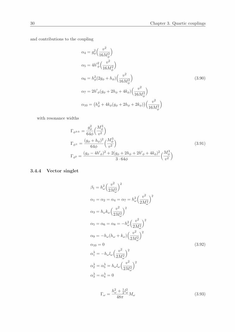
30 Chapter 3. Quartic couplings
and contributions to the coupling
α4 = g2φ
( v2
16M2φ
)
α5 = 4h′2φ( v2
16M2φ
)
α6 = h2φ(2gφ + hφ)
( v2
16M2φ
)(3.90)
α7 = 2h′φ(gφ + 2hφ + 4kφ)( v2
16M2φ
)
α10 =(h2φ + 4kφ(gφ + 2hφ + 2kφ)
)( v2
16M2φ
)
with resonance widths
Γφ±± =g2φ
64φ
(M3φ
v2
)
Γφ± =(gφ + hφ)2
64φ
(M3φ
v2
)(3.91)
Γφ0 =(gφ − 4h′φ)2 + 2(gφ + 2hφ + 2h′φ + 4kφ)2
3 · 64φ
(M3φ
v2
)
3.4.4 Vector singlet
β1 = h2ω
( v2
2M2ω
)2
α1 = α2 = α4 = α7 = h2ω
( v2
2M2ω
)2
α3 = hωkω
( v2
2M2ω
)2
α5 = α6 = α8 = −h2ω
( v2
2M2ω
)2
α9 = −hω(hω + kω)( v2
2M2ω
)2
α10 = 0 (3.92)
αλ1 = −hωlω( v2
2M2ω
)2
αλ2 = αλ5 = hωlω
( v2
2M2ω
)2
αλ3 = αλ4 = 0
Γω =h2ω + 1
2 l2ω
48πMω (3.93)
31
3.4.5 Vector triplet
β1 = 4h2ρ(gρ + hρ)
v2
2M2ρ
− (gρ + 2hρ)2v2∆M2
ρ
2M4ρ
α1 = (gρ + 2hρ)2( v2
2M2ρ
)2
α2 = [−gρ(gρ(1− µ′ρ) + 2kρ
)+ 4h2
ρ]( v2
2M2ρ
)2
α3 = (gρ + 2hρ)[gρ(1 + µρ) + k′′ρ]( v2
2M2ρ
)2
α4 = −α5 = (gρ − 2hρ)2( v2
2M2ρ
)2(3.94)
α6 = −α7 = 8gρhρ( v2
2M2ρ
)2
α8 = −4hρ(gρ + hρ)( v2
2M2ρ
)2
α9 = −[(2hρ + k′′ρ)(gρ + 2hρ) + 2hρ(k′ρ + gρµρ)]( v2
2M2ρ
)2
α10 = 0
αλ1 = −[(gρ + 2hρ)(lρ + 2l′′ρ) + 2gρlρ]( v2
2M2ρ
)2
αλ2 =[(gρ + 2hρ)(lρ + 2l′′ρ)− cW
sWgρl
′ρ
]( v2
2M2ρ
)2
αλ3 = −(gρ + 2hρ)lρ( v2
2M2ρ
)2(3.95)
αλ4 = −cWsW
(gρ + 2hρ)l′ρ( v2
2M2ρ
)2
αλ5 = −(gρ + 2hρ)l′′ρ( v2
2M2ρ
)2
Γρ± =(gρ) + 2hρ)2 + 2l2ρ + 1
2 l′2ρ
48πMρ
Γρ0 =(gρ)− 2hρ)2 + 2(lρ + 2l′′ρ)2
48πMρ (3.96)

32 Chapter 3. Quartic couplings
3.4.6 Tensor singlet
α4 = g2f
( v2
8M2f
)
α5 = −g2f
4
( v2
8M2f
)
α6 = 2gfhf( v2
8M2f
)(3.97)
α7 = −gfhf2
( v2
8M2f
),
α10 =3h2
f
2
( v2
8M2f
)
Γf =g2f + 1
2(gf + 2hf )2
16π
( M3f
30v2
)(3.98)
where two terms in the numerator correspond to the partial widths to WW and ZZ,respectively.
3.4.7 Tensor triplet
α4 = h′2a( v2
8M2a
)
α5 = −h2a
4
( v2
8M2a
)
α6 =14
(12h2a + 4h′a(ha + 2ka)
)( v2
8M2a
)(3.99)
α7 =14(h2a − h′a(ha + 2ka)
)( v2
8M2a
)
α10 =3ka(ha + ka)
2
( v2
8M2a
)
and for the widths
Γa± =h2a
64π
( M3a
30v2
)
Γa0 =h′2a
12(ha + h′a + 2ka)2
16π
( M3a
30v2
)(3.100)

33
3.4.8 Tensor quintet
α4 =(14g2t + 4h′2t
)( v2
16M2t
)
α5 =(12g2t − h′2t
)( v2
16M2t
)
α6 =(1
2h2t
(gt +
12ht
)+ 4h′t
(12gt + ht + 2kt
))( v2
16M2t
)(3.101)
α7 =(h2t
(gt +
12ht
)− h′t(12gt + ht + 2kt
))( v2
16M2t
)
α10 = 3(1
4h2t + kt
(gt + ht + 2kt
))( v2
16M2t
)
where widths are
Γt±± =g2t
64π
( M3t
30v2
)
Γt± =(gt + ht)2
64π
( M3t
30v2
)(3.102)
Γt0 =13
(gt − 4h′t)2 + 2(gt + 2ht + 2h′t + 4kt)2
64π
( M3t
30v2
)

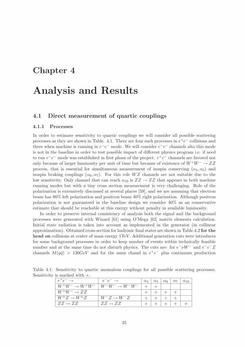
Chapter 4
Analysis and Results
4.1 Direct measurement of quartic couplings
4.1.1 Processes
In order to estimate sensitivity to quartic couplings we will consider all possible scatteringprocesses as they are shown in Table. 4.1. There are four such processes in e+e− collisions andthree when machine is running in e−e− mode. We will consider e−e− channels alto this modeis not in the baseline in order to test possible impact of different physics program i.e. if needto run e−e− mode was established in first phase of the project. e+e− channels are favored notonly because of larger luminosity per unit of time but because of existence of W+W− → ZZprocess, that is essential for simultaneous measurement of isospin conserving (α4, α5) andisospin braking couplings (α6, α7). For this role WZ channels are not suitable due to thelow sensitivity. Only channel that can reach α10 is ZZ → ZZ that appears in both machinerunning modes but with a tiny cross section measurement is very challenging. Role of thepolarization is extensively discussed at several places [59], and we are assuming that electronbeam has 80% left polarization and positron beam 40% right polarization. Although positronpolarization is not guaranteed in the baseline design we consider 40% as an conservativeestimate that should be reachable at this energy without penalty in available luminosity.
In order to preserve internal consistency of analysis both the signal and the backgroundprocesses were generated with Wizard [61] using O’Mega [62] matrix elements calculation.Initial state radiation is taken into account as implemented in the generator (in collinearapproximation). Obtained cross-section for hadronic final states are shown in Table.4.2 for thehead on collisions at center of mass energy 1TeV. Additional generation cuts were introducesfor some background processes in order to keep number of events within technically feasiblenumber and at the same time do not disturb physics. The cuts are: for e−νW− and e−e−Zchannels M(qq) > 130GeV and for the same chanel in e+e− plus continuum production
Table 4.1: Sensitivity to quartic anomalous couplings for all possible scattering processes.Sensitivity is marked with +.
e+e− → e−e− → α4 α5 α6 α7 α10
W+W− →W+W− W−W− →W−W− + +W+W− → ZZ + + + +W±Z →W±Z W−Z →W−Z + + + +ZZ → ZZ ZZ → ZZ + + + + +
35

36 Chapter 4. Analysis and Results
Table 4.2: Generated processes and cross sections of signal and background for√s = 1TeV,
polarization 80% left for electron and 40% right for positron beam
Channel σ[fb] Channel σ[fb]e+e− → νeνeW
+W− → νeνeqqqq 23.19 e−e− → νeνeW−W− → νeνeqqqq 27.964
e+e− → νeνeZZ → νeνeqqqq 7.624 e−e− → e−νeW−Z → e−νeqqqq 80.2e+e− → ννqqqq (3V contribution) 9.344 e−e− → e−e−ZZ → e−e−qqqq 3.16e+e− → νeWZ → νeqqqq 132.3 e−e− → e−e−W+W− → e−e−qqqq 443.9e+e− → e+e−ZZ → e+e−qqqq 2.09 e−e− → e−e−tt→ e−e−X 0.774e+e− → e+e−W+W− → e+e−qqqq 414.6 e−e− → ZZ → qqqq 232.875e+e− → tt→ X 331.768 e−e− → e−νeW− → e−νeqq 235.283e+e− →W+W− → qqqq 3560.108 e−e− → e−e−Z → e−e−qq 125.59e+e− → ZZ → qqqq 173.221e+e− → eνW → eνqq 279.588e+e− → e+e−Z → e+e−qq 134.935e+e− → qq → X 1637.405
e+e− → qq of M(qq) > 140GeV . All 2,4 and 6 fermion final states were generated directly(there is no on-shell production and subsequent decay) so natural width of the weak bosons isproperly taken into account. Events were generated with SM values for the quartic couplingi.e. αi ≡ 0, i ∈ {4, 5, 6, 7, 10}. Triple couplings were also set to SM values since we assumethat even if the deviations to the SM value are observed they are measured with precision thatis well above one that we can reach for the quartic ones so taking any well known number forvalue of triple couplings is equivalent.
Fragmentation and hadronization of quark final states was done by Pithya [71] beforepassing the event to the detector simulation. Detector response was simulated with Simdet[63], fast parametric Monte Carlo program based on th full detector simulation of TESLAdetector [7].
4.1.2 Observable
There are several observable that are sensitive to the deviation of chiral coupling from theirSM values. First is the total cross section. Example for that dependence are shown in Fig.4.1for most important processes. From the low energy measurements values of the couplings arealready constrained1 to the level that total variation of the cross section is on the order of 1%asking for very good cross section calculation. Due to the dependence of all processes on atleast two couplings cross section cannot be used as an exclusive variable since the solution of theproblem σ(αi) = σSM is ellipse in the parameter plane (two dimensional case) or hypersurfacein parameter space (three and more dimensional case). This point is important since it stressesthe fact that this is not a simple counting experiment! Other variables are needed tobrake the symmetry of the solution. Since expected new effects should manifest them selves onthe scale well above direct reach of the collider and we are lookin only at lower energy remnantof that mechanism the closer we are to that scale effects should be larger. Thus mass of theevent is another sensitive variable. Unfortunate is that in all scattering processes we have twoleptons that are carrying significant fraction of the momentum away and reducing the effective
1putting a side all more or less founded complains against those numbers

37
Figure 4.1: Cross section dependence on quartic couplings for ννW+W− process on the left,and ννZZ on the right.
center of mass energy. Events with high mass should be more sensitive to the possible deviationin quartic couplings form SM values. Information about SBS should be carried primarily withlongitudinally polarized weak bosons and their interaction thus production and decay anglesare also sensitive variables. Since there is no distinction between weak bosons or quark antiquark these distributions are folded reducing the sensitivity to and extent. Sensitivity tomentioned variables is demonstrated on Fig.4.2 withe ratio of mentioned distributions forα4 = 4 to the SM ones for ννW+W− process.
4.2 Event selection
Since we are dealing with several processes with significant similarities common analysis issuesand essential steps for the analysis will be explained once for all the processes in question.Event selection was largely based on the previous analysis [83] that was done at 800GeV sothere will be some referring to the 800GeV-1TeV differences, and all the selection criteria arerevisited and changed if necessary. After that overview of applied selection criteria will bepresented with summary of obtained results.
4.2.1 Jet pairing
During the second run of the LEP experiment significant problem for the analysis was the jetpairing. This problem has risen out of the several raison running close to the threshold forthe weak boson pair production leads to the jets with no or very small bust and then withjets with large opening angles ( [65]) that are prone to the reassignment of particles with thejet algorithm. Appropriate complex procedures were developed for dealing with such effects[66]. At higher energies we are in much better situation since jets are more collimated due tothe significant boost with almost no back flying particles making easier task for the jet findingalgorithm. Second important change is the precision of the measurement of the momenta andthe directions of the particles reducing the overall smearing of the topology.
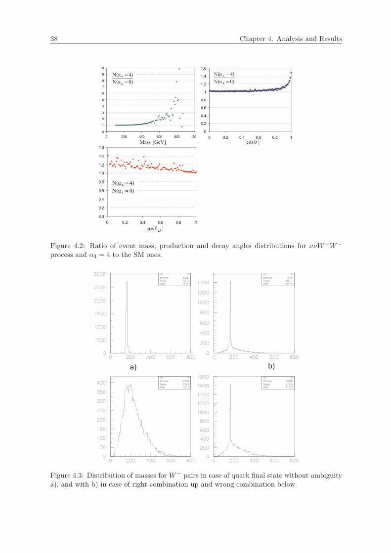
38 Chapter 4. Analysis and Results
Figure 4.2: Ratio of event mass, production and decay angles distributions for ννW+W−
process and α4 = 4 to the SM ones.
a) b)
Figure 4.3: Distribution of masses for W− pairs in case of quark final state without ambiguitya), and with b) in case of right combination up and wrong combination below.

39
a) b)
Figure 4.4: Distribution of masses for W− pairs in case of quark final state without ambiguitya), and with b) in case of right combination up and wrong combination below after correction.
W−W− → q q q q
1 2 3 4 (4.1)
Optimal pairing is anyhow still a important step in any multi jet final state analysis. Wayto the optimal pairing is to know the true right pairing and then to develop the procedure tomaximize the right output. Since Whizard is N-fermion generator and due to the lack of thecolor information there were tiny issues about the knowledge of the right quark color singletpairs at the output. At the output we have four quarks, and lets enumerate them from 1 to 4as in eq.4.1. In some of the final states like for W− pairs like dUsC the right pairing is dU andsC, in some case like dUdU there is possibility that singles are not expected combination 1-2and 3-4 but 1-4 and 2-3. In order to test this mass distributions were made for both final cases,in the way that expected “right” pairing (1-2,3-4) was put in one histogram and other two“wrong” combinations in another. This procedure was repeated for final states were ambiguitydoes not exist and in those were it is possible. In the Fig.4.3 findings are summarized. Casea) shows no ambiguity case with correct combination on upper and two other combinationon lower plot. Case b) shows final state with ambiguity and lower plot clearly indicates thatin half of the combination right pairing is 1-4 2-3. Using the information about the naturalwidth of the mass distribution and it’s shape i.e. Bright-Wiegner it was possible to correct forthis effect. In Fig.4.4 are same distribution after correction. Now they look absolutely similar.Correction procedure was used in all situations were ambiguity could have existed due to thespecific treatment of the events i.e. their fragmentation calling Pithya routine PY4FRM with

40 Chapter 4. Analysis and Results
pairing mass window +abs diff. full N right eff[%] σ[GeV ]original 3367 3266 2798 2730 97.57 3.33(10)χ2 3954 3837 3262 3167 97.09 3.34(10)
gauss 5007 4892 4328 4127 95.36 3.46(9)IBW Γ = 5GeV 4992 4870 4322 4121 95.35 3.45(9)IBW Γ = 4GeV 4989 4863 4317 4117 95.37 3.45(9)IBW Γ = 3GeV 4926 4855 4312 4114 95.41 3.44(9)
Table 4.3: Pairing method optimization for ν channel
the flag to stick to the user defined pairing since the routine would use ordinary WW andZZ pair production matrix elements otherwise. At this stage we have assured that we knowthe right quark pairs at the start. Now we will revisit the pairing criteria used in the TDRanalysis, initial pairing condition was to us eq. 4.2.
Min(|Mi −MV | |Mj −MV |) (4.2)
where Mi and Mj are masses of the jet pairs and MV is mass of the weak boson (eider Wor Z). Noticed disadvantage of the chosen criteria is that due to the structure of the functionit strongly prefers one pair exact or very close to the nominal mass and the second can bealmost anything. Three addition possible measures were introduced trying to remedy thiskind of behavior. One is usual χ2 measure as in eq.4.3
Min((Mi −MV )2
σ2+
(Mj −MV )2
σ2) (4.3)
and two principally new exploiting excellent performance of the ILC detector 2.
Min(exp (Mi −MV
σ)2 exp (
Mj −MV
σ)2) (4.4)
Min((M2
V −M2i )
2 +M2V Γ2
Γ2
(M2V −M2
j )2 +M2
V Γ2
Γ2) (4.5)
Both are base on the fact that initial mass distribution of the weak boson defined byBreight-Wiegner shape (ΓW = 2.124GeV and ΓZ = 2.2952GeV ) is preserved by the detectorresolution leading to the same distribution for probability density function of reconstructedjet pairs around nominal mass, understandable with higher width. Since this distribution isin fact in the transition region between the gauss and BW (natural and detector contributionto the final width are comparable) both dependences were tested. Condition from eq.4.4we will call simply Gauss, and from eq.4.5 inverse breight-wiegner (IBW). Note that due tothe structure of the functions both χ2 and Gauss do not depend on the used σ, formallyvalue of the function is scaled but the position of the minimum is not moved. For the IBWdistribution this is not the case since width is entering on both sides of the fraction thus itis possible, although for small fraction of the events, that with different used width differentpairing combination has the minimum of the function.
Test sample contains the 10000 events for the WW process.In Tab.4.2.1 we summarize pairing optimization. All other selection cuts are applied except
the cuts on the mass of the single weak bosons and pairs. Additional cuts are mass of one2By detector performance always assume combined hardware and reconstruction software performance

41
Pt mass [GeV] 2.0 2.1 2.2 2.3 2.4 2.5 2.6 2.7 2.8 2.9duuu (dudd) 3 3 3 3 3 2 2 2 2 2
sccc 29 23 23 22 20 19 19 18 16 16dubb 392 384 371 351 339 332 323 317 308 290
Table 4.4: Number of events passing the condition at least one jet with vertex mass above.Samples of 500 events with specified final state.
candidate should be 65GeV < Mi < 88GeV called mass window in the table, differencebetween candidate masses should be |Mi−Mj |< 20GeV called absolute difference this cut isapplied additionally to the mass window cut. Finally third cut is applied 148GeV < Mi+Mj <172GeV , together with previous two, and passed number of events is in column full. Using thetrue information number of event with correct pairing is calculated and is in column N right.Efficiency of correct pairing after the selection cuts is then calculated and the distribution isfitted with Gauss function plus second order polynome (to account for possible combinatorialbackground). Both new pairing conditions give significantly higher yeld with minimal dropof 2%in correct pairing efficiency. Obtained width is for all methods is consistent within thefit errors and exactly with the prediction. Results for the Gaussian and IBW approach arestatistically equivalent after applied cuts further on eq.4.5 was used as a pairing condition.Durham algorithm was used as a jet algorithm of the choice as it has shown best performance,as already concluded in extensive studies [67]. Tuning of the algorithm can affect efficiencyonly on the 1% level.
4.2.2 B tagging
For same fraction of interesting processes final states as well for the background expectedexcellent b-tagging capability of ILC detector [68] is valuable additional information for theseparation of the signal and the background. In the fast simulation integrated tools allowedusage of the ZVTOP algorithm [70] for the b-tagging. Originally the final b-tag was madeusing the neural network that was trained at Zpole [69]. We have tried to keep the analysis biasfree as possible thus usage of such network was not an option, as well as retraining the networkwith ∼ 107 events needed (that is larger then our total event sample). Instead of network onlytransverse momentum corrected vertex mass was used for b-tag. Event has positive b-tag ifcontains at least one jet with vertex of mass aboveMcut. In order to determine needed cut valuefinal states of W±Z were divided to subsamples containing only light quark combinations,charm and strange, and sample with Z → bb decay as in Table.4.2.2 and range of Mcut from2.0-2.9GeV was tested. Following original SLD result (as on Fig.4.5) and our test value ofMcut = 2.1GeV was chosen as appropriate that is giving 77% efficiency for identification andless then < 2.5% of fakes. Importance of suppression for Z → bb channel is large due to thefact that increased amount of neutrinos in decay chain is shifting reconstructed mass to lowervalues increasing contamination within W mass window in respect to the amount anticipatedon the base of reconstruction performance alone. It also aloes to suppers contamination ofsame final state from different processes like in eνWbb case where we can have two paths, oneform e±νW∓Z → e±νW∓bb and second from tt→W+W−bb that with one decay W± → e±νleads to the same final state. Identification of b jets allows additional mass cut on the rightcombination of jets and elimination of SM background.

42 Chapter 4. Analysis and Results
Figure 4.5: Pt corrected mass distribution, with the line and an error cut used in the analysisis marked.
Figure 4.6: Angular coverage of detector elements as implemented in fast simulation. Numbersare cosines of the lowest angle covered by the region.
4.2.3 Forward region
All the processes under consideration can be splitted into two groups on the existence ornonexistence of lepton in the final state. This feature can be used to increase signal back-ground separation and separation between signals. At high energies all distributions becomeincreasingly forward peaked thus it is of significant importance to have reliable tag up tolowest possible angle. In Fig.4.6 we have a sketch of detector coverage in the forward regionas implemented in fast simulation.
TPC edge was set to 12degrees that obviously assumes full vertex support. Tracking isassumed to work till 7 degrees. Below that we hade part of the ECAL, LAT and LCAL withtheir angular coverage as in TDR. So no charge information was available below 7 degrees plusbelow lower edge of the ECAL all measured particles were “identified”as photons (probablywith raison that these are electromagnetic calorimeters). Detailed background studies donefor that part of the detector at that time have shown that reconstruction thresholds for that
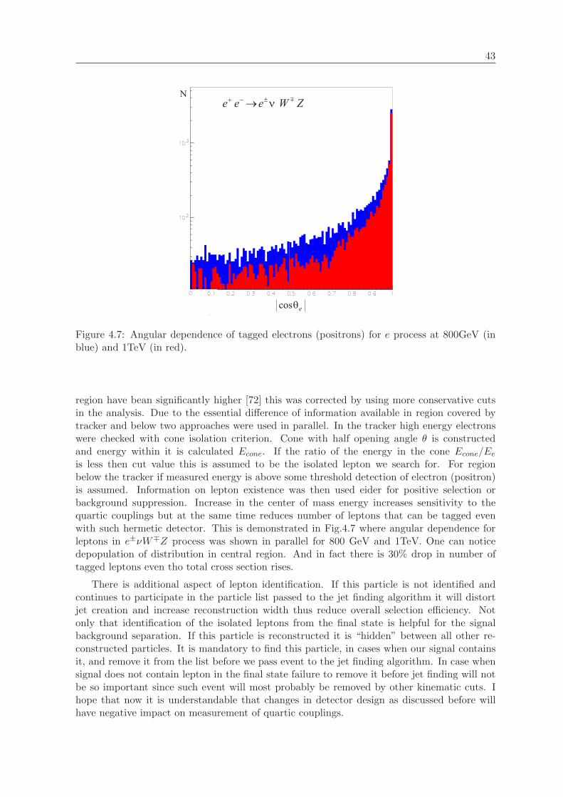
43
Figure 4.7: Angular dependence of tagged electrons (positrons) for e process at 800GeV (inblue) and 1TeV (in red).
region have bean significantly higher [72] this was corrected by using more conservative cutsin the analysis. Due to the essential difference of information available in region covered bytracker and below two approaches were used in parallel. In the tracker high energy electronswere checked with cone isolation criterion. Cone with half opening angle θ is constructedand energy within it is calculated Econe. If the ratio of the energy in the cone Econe/Eeis less then cut value this is assumed to be the isolated lepton we search for. For regionbelow the tracker if measured energy is above some threshold detection of electron (positron)is assumed. Information on lepton existence was then used eider for positive selection orbackground suppression. Increase in the center of mass energy increases sensitivity to thequartic couplings but at the same time reduces number of leptons that can be tagged evenwith such hermetic detector. This is demonstrated in Fig.4.7 where angular dependence forleptons in e±νW∓Z process was shown in parallel for 800 GeV and 1TeV. One can noticedepopulation of distribution in central region. And in fact there is 30% drop in number oftagged leptons even tho total cross section rises.
There is additional aspect of lepton identification. If this particle is not identified andcontinues to participate in the particle list passed to the jet finding algorithm it will distortjet creation and increase reconstruction width thus reduce overall selection efficiency. Notonly that identification of the isolated leptons from the final state is helpful for the signalbackground separation. If this particle is reconstructed it is “hidden” between all other re-constructed particles. It is mandatory to find this particle, in cases when our signal containsit, and remove it from the list before we pass event to the jet finding algorithm. In case whensignal does not contain lepton in the final state failure to remove it before jet finding will notbe so important since such event will most probably be removed by other kinematic cuts. Ihope that now it is understandable that changes in detector design as discussed before willhave negative impact on measurement of quartic couplings.

44 Chapter 4. Analysis and Results
4.2.4 Overview of selection criteria
e−e− → ννW−W−
If one considers what distinct this from other signal channels that are two features . No leptonsin final state and no b-quarks in the final state. Exactly from this general considerationsselection starts. All reconstructed particles are checked for electrons (positrons) or highlyenergetic object in the region below the tracker. Some minimal electron energy must betaken as threshold for this consideration since existence of higher energy electrons withinjets although not so probable is still possible. So lower energy for the electron cut is set toEecut > 18.0GeV . For tracker we construct a cone with half opening angle of 7.5 degrees andcollect energy within it. Ratio of the energy in the cone Econe and the energy of electron ismade if
EconeEe±
< 0.25 (4.6)
we consider lepton isolated and reject the event. In low angle region that is not coveredby tracker rejection was made only on the base of energy. If object is above 70GeV in LATor corner region of ECAL, or above 100GeV in LCAL. If passed event is forced to 4 jets.B-tagging code is called and number of jets with vertex mass over 2.1GeV is counted. If anysuch found event is rejected. After weak preselection requiring that we have at least 7 chargedtracks and 10 reconstructed objects kinematic variables are calculated. First the total visiblemomentum P of the event as usual vector sum
Pj =∑
pij j = x, y, z, E (4.7)
from this we calculate transverse momentum and total mass
Ptr =√P 2
1 + P 22 , M2
tot = P 24 −
3∑
i=1
P 2i (4.8)
missing energy simply by Emiss = 1TeV − P4
and transverse energy and missing mass
Etr =∑
Ei sin θi , M2miss = E2
miss −3∑
i=1
P 2i (4.9)
and absolute value for the cosine of missing momentum
cos θmiss =Abs(P3)| P | (4.10)
Following cuts values were used (if condition is satisfied event is accepted) Ptr > 35GeV150 < Etr < 600GeV , Mmiss > 200GeV , Emiss > 200GeV and cos θmiss < 0.99. For eventsthat survived so far jet pairing is done using IBW function with Γ = 3GeV and final cuts onthe mass variables were made. Mass window for W mass 60 < MW < 88GeV , cut on the sumof the two masses 140 < MW1 + MW2 < 172GeV and constrain that reconstructed massesshould not have large difference | MW1 −MW2 |< 20GeV . Numbers in the mass subscriptsjust label that there are two reconstructed W boson no ordering is done what so ever. For theevents that have passed this final cuts sensitive variables were calculated and stored.
In Table.4.5 final numbers of events after explained selection is shown. Al the numbersin the table are estimates for 1ab−1 although signal process is always processed with higherstatistics (8x in this case). As one would expect the more similar background channel is tothe signal the more we accept. One can wonder why have we accepted such numbers as finalwith signal to background of the order of 2 (2.08).
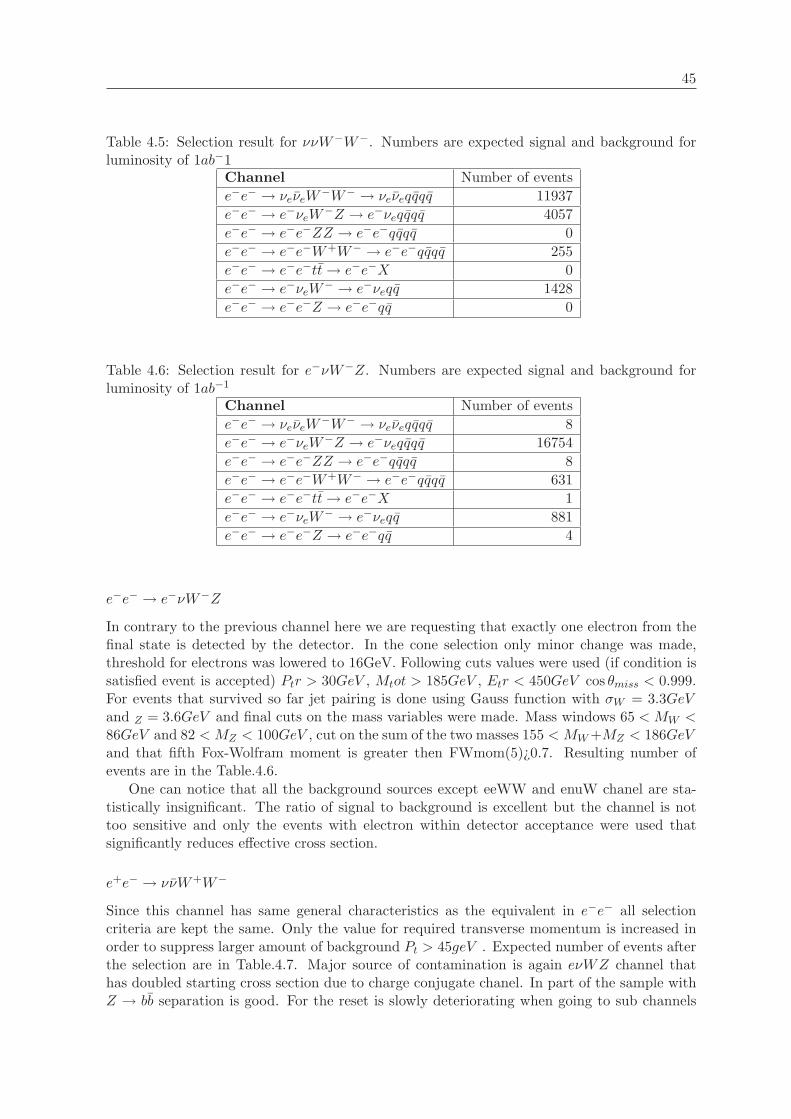
45
Table 4.5: Selection result for ννW−W−. Numbers are expected signal and background forluminosity of 1ab−1
Channel Number of eventse−e− → νeνeW
−W− → νeνeqqqq 11937e−e− → e−νeW−Z → e−νeqqqq 4057e−e− → e−e−ZZ → e−e−qqqq 0e−e− → e−e−W+W− → e−e−qqqq 255e−e− → e−e−tt→ e−e−X 0e−e− → e−νeW− → e−νeqq 1428e−e− → e−e−Z → e−e−qq 0
Table 4.6: Selection result for e−νW−Z. Numbers are expected signal and background forluminosity of 1ab−1
Channel Number of eventse−e− → νeνeW
−W− → νeνeqqqq 8e−e− → e−νeW−Z → e−νeqqqq 16754e−e− → e−e−ZZ → e−e−qqqq 8e−e− → e−e−W+W− → e−e−qqqq 631e−e− → e−e−tt→ e−e−X 1e−e− → e−νeW− → e−νeqq 881e−e− → e−e−Z → e−e−qq 4
e−e− → e−νW−Z
In contrary to the previous channel here we are requesting that exactly one electron from thefinal state is detected by the detector. In the cone selection only minor change was made,threshold for electrons was lowered to 16GeV. Following cuts values were used (if condition issatisfied event is accepted) Ptr > 30GeV , Mtot > 185GeV , Etr < 450GeV cos θmiss < 0.999.For events that survived so far jet pairing is done using Gauss function with σW = 3.3GeVand Z = 3.6GeV and final cuts on the mass variables were made. Mass windows 65 < MW <86GeV and 82 < MZ < 100GeV , cut on the sum of the two masses 155 < MW+MZ < 186GeVand that fifth Fox-Wolfram moment is greater then FWmom(5)¿0.7. Resulting number ofevents are in the Table.4.6.
One can notice that all the background sources except eeWW and enuW chanel are sta-tistically insignificant. The ratio of signal to background is excellent but the channel is nottoo sensitive and only the events with electron within detector acceptance were used thatsignificantly reduces effective cross section.
e+e− → ννW+W−
Since this channel has same general characteristics as the equivalent in e−e− all selectioncriteria are kept the same. Only the value for required transverse momentum is increased inorder to suppress larger amount of background Pt > 45geV . Expected number of events afterthe selection are in Table.4.7. Major source of contamination is again eνWZ channel thathas doubled starting cross section due to charge conjugate chanel. In part of the sample withZ → bb separation is good. For the reset is slowly deteriorating when going to sub channels

46 Chapter 4. Analysis and Results
Table 4.7: Selection result for ννW+W−. Numbers are expected signal and background forluminosity of 1ab−1
Channel Number of eventse+e− → νeνeW
+W− → νeνeqqqq 9279e+e− → νeνeZZ → νeνeqqqq 332e+e− → νeWZ → νeqqq 2878e+e− → e+e−ZZ → e+e−qqqq 0e+e− → e+e−W+W− → e+e−qqqq 0e+e− → tt→ X 8e+e− →W+W− → qqqq 1262e+e− → ZZ → qqqq 29e+e− → eνW → eνqq 1374e+e− → e+e−Z → e+e−qq 0e+e− → qq → X 180
with heavier quark combination.One can be surprised about the number of event accepted from single W production but
you should not forget that only far off shell part of that process was generated anyhow andthat this channel has total cross section orders of magnitude higher then the signal. The samesituation is with WW process where from millions of events half permile still looks like signal.Since contamination over the final states rises to heavy quark combination emission of highenergy neutrinos is probably responsible for the effect. All the remaining contribution areprobably negligible. Again with tighter cuts it is possible to get better signal to backgroundratio but fit was telling us that it is more important to keep significant part of the signal thento have more pure sample.
e+e− → eνWZ
All the parameters used in the selection are the same as for e−e− reaction with minor changes.Cut on the transverse momentum was adjusted to Pt > 25GeV . Difference in the tagging ofthe final state lepton is that here we cannot ask for the exact charge so electrons and positronsare treated equivalently. Difference is also that the final state of the form eνW±bb can bereached from the tt state but as one can see in the Table.4.8 no significant contribution isobserved.
e+e− → ννZZ
Preselection in this chanel contains only final state lepton suppression. Energy threshold forcone method is raised to 20GeV. For the pairing Gaussian condition is used with width of3.6GeV. Remaining cuts on the kinematic variables are Mmiss > 220GeV , Etr > 175GeV ,200 < Emiss < 750GeV ,cos θmiss < 0.999. and thrust value of the event should be less then0.91. Final mass cuts are 85 < MZ < 100GeV , 171 < MZ1 + MZ2. After event selectionestimated number of events is presented in Table.4.9.
As expected major backgrounds are ννWW and eνWZ channels. Separation is hardsince mentioned channels have significantly larger cross sections. Effectively only variablethat produces separation is the mass. But due to the low starting number of events tightercut would reduce already low number of events. Several options with likelihood approach for

47
Table 4.8: Selection result for e±νW∓Z. Numbers are expected signal and background forluminosity of 1ab−1
Channel Number of eventse+e− → νeνeW
+W− → νeνeqqqq 30e+e− → νeνeZZ → νeνeqqqq 21e+e− → νeWZ → νeqqq 15022e+e− → e+e−ZZ → e+e−qqqq 14e+e− → e+e−W+W− → e+e−qqqq 629e+e− → tt→ X 167e+e− →W+W− → qqqq 440e+e− → ZZ → qqqq 121e+e− → eνW → eνqq 1253e+e− → e+e−Z → e+e−qq 20e+e− → qq → X 85
Table 4.9: Selection result for ννZZ. Numbers are expected signal and background forluminosity of 1ab−1
Channel Number of eventse+e− → νeνeW
+W− → νeνeqqqq 1505e+e− → νeνeZZ → νeνeqqqq 2485e+e− → νeWZ → νeqqq 4301e+e− → e+e−ZZ → e+e−qqqq 0e+e− → e+e−W+W− → e+e−qqqq 319e+e− → tt→ X 49e+e− →W+W− → qqqq 309e+e− → ZZ → qqqq 68e+e− → eνW → eνqq 763e+e− → e+e−Z → e+e−qq 0e+e− → qq → X 85

48 Chapter 4. Analysis and Results
separation were tested without significant improvement.
e−e− → e−e−ZZ and e+e− → e+e−ZZ
Both channels have one distinct feature in common that is two leptons in the final state. Inaddition they have smallest cross section of all signal processes. Since it is from the start clearthat there will not be decent statistics for the signal event selection was made with differentfocus. We try to bring all the background to 0 level and see is there any signal event left. Itis possible to suppress background fully, but for the e−e−ZZ process we have extracted 28events from 8ab−1. For e+e−ZZ situation is similar ( 31 event in 10ab−1). In addition thatsignal part of the e+e−ZZ we also have contribution from the triple weak boson productionand since one is forced to put Z mass constrain on lepton pair no scattering events wereextracted. In order to have any hope of separating this from eeWW channel b-tagging is mustsuppression of background required to restrain ourselves to at least ZZ → xxbb. Selectionfor e−e− requires two isolated leptons. Cut for the threshold energy for such consideration israised to 20GeV. Pairing is one width Gaussian function with σ = 3.6GeV . Missing energybefore tagged leptons removal should be Emiss < 240GeV , there should be at least two jetswith b-tag. Total mass of the event Mtot > 200GeV and cos θmiss < 0.996 were also used.Final mass constraints are 83 < MZ < 100GeV and 172 < MZ1 +MZ2 < 191GeV . For e+e−
there is additional cut that | Mee −MZ |< 5GeV . Thus there are enough events to formallyextract the value but one should be cautious with interpretation of the result. What is beyondany dough that this channel is on the edge of detection.
4.3 Quartic couplings extraction
If quartic couplings deviate from the expected SM values we hope to see deviation in someof the distributions that are sensitive to them. Extracting of their values can proceed inat least two ways. One would be to generate another sample of events with ~α 6= ~α(SM)construct wanted distributions and then extract sensitivity. In case of only one free variablethis would be fully acceptable, but we have multi parameter space with variables coming inlinear combinations that makes such approach highly tedious. Second possibility is to assignweight to the event depending on the coupling and use re-weighted distributions for the fit.Since Whizard-O’Mega combination support recalculation of the matrix element for alreadygenerated events if one of the parameters is changed (in our case anomalous couplings) we willuse this approach.
How should the weights look like? For the signal processes we have the part of the matrixelement that is not dependent on the quartic couplings, in some sense SM background, andnon SM part linear in αi in total:
Mtotal = MSM +Mα (4.11)
leading to the quadratic dependence of squared matrix element on αi:
MtotalM∗total = (MSM +Mα)(MSM +Mα)∗
= MSMM∗SM +MSMM
∗α +M∗
SMMα +MαM∗α
= 1 +O(α) +O(α2) (4.12)
Taking this into account weight for the events were chosen to have following, quadratic, form:
R(αi, αj) = 1 +Aαi +Bαi2 + Cαj +Dαj
2 +Eαiαj (4.13)

49
Table 4.10: Evaluation shema for extraction of weight coefficients.N αi αjR1 +a 0R2 −a 0R3 0 +aR4 0 −aR5 +a +a
where coefficients A to E should be determined on event by event basis and αi, αj stands forquartic couplings or their linear combinations. We need 5 point with different value for thecoupling in order to extract weight coefficients A to E. The points were chosen according tothe shema in Table. 4.10, where “a” i particular value of the coupling. Once we have weightsR1 to R5 solving the system of linear equations gives the coefficients:
A =R1 −R2
2a
B =R1 +R2 − 2
2a2
C =R3 −R4
2a(4.14)
D =R3 +R4 − 2
2a2
E =R5 −R1 −R3 + 1
a2
Choice of “a” is important since it must satisfy some conditions. Re-weighting method isbased on the assumption that phase space for the generation of the events has not changedmuch (there are no peaks just scaling) so that the regeneration of the events is not needed thuslarge values of the parameter “a” must be avoided since they could correspond to the situationwhere this assumption is not valid any more. Extremely small values of the parameter “a”should be also avoided for precision raison since matrix element recalculation was limited to adouble precision and we have differences of close by numbers in eq.4.14. As an optimal choicevalue of 1 i.e 1/16π was taken for the calculation (increased to 3 for the low sensitivity channellike e±νW∓Z to avoid mentioned problems). For all events of the signal processes coefficientswere calculated and stored. After selection of the events coefficients for selected events areused in the fit.
Measurement sensitivity was evaluated using binned likelihood minimized using Minuit[64]. Particular care was taken with binning. Formally with increase of the number of binsthe precision would rise, but it could lead to the situation when the number of events per binis such that statistics assumed for construction of the likelihood is not valid any more andto the wrong results. Over binning shows itself in unstable results with respect to the smalladjustment of the bin position and in the jumps of the global minima to the isolated localminima far form the SM expectation value. Number of bins was adjusted in such a way tomaximize the sensitivity by keeping the constrain of min number of events in bin at the orderof 10.
L(αp, αq) = −∑
i,j,k,l
NSM (i, j, k, l) ln (Nαp,αq(i, j, k, l)) +∑
i,j,k,l
Nαp,αq(i, j, k, l) (4.15)

50 Chapter 4. Analysis and Results
Figure 4.8: Stability of the quartic couplings extraction procedure for ννW−W− process. Indark blue 50% CL, in light blue 95%CL, six “measurements” with 1σ errors on top of it onthe left. Consistency of obtained result for ν+W− channel at 800GeV in green, and 1TeV red,70% CL in full, 95% CL dotted.
where bins (i,j,k,l) are over mass of the event, production and two decay angles. Standardmodel expectation is plain sum of the number of events in the binNSM (i, j, k, l) =
∑R(0, 0) =∑
1 and the Nαp,αq(i, j, k, l) =∑R(αp, αq) is the sum of the re-weighted events in the same
bin. Since we are interested in the sensitivity of the measurement and not the outcome for theparticular dataset, signal events were generated with significantly larger statistics (∼ 10x) thenone expected. The likelihood was then appropriately scaled down to the nominal luminosity.Naturally this kind of procedure rises question of the result stability and possible systematiceffects introduced by it. This dough were eliminated by following test in the early stageof analysis. Large signal sample was first passed through the analysis chain and the limitfor the couplings were extracted (by scaling down the likelihood to 1ab−1) . The samplewas then splitted in subsamples with nominal luminosity 1ab−1 in such a way that in thefitting this part of the sample is not participating thus removing the possible bias from usageof the same events. This was done for 6 subsamples. The result is in the Fig.4.8 for thee−e− → ννW−W− process. We see that spread of “measurement” points fits well with theextracted confidence level contours and that the procedure is making reliable sensitivity limitsprediction. Additional confirmation to the reliability of results is there is no intersection ofconfidence level contours obtained at different energies demonstrated on ννW+W− processon the same figure. Never the less thigh to remember is that procedure is not giving the resultof a particular measurement but sensitivity limits for large number of such measurements!
Here we should also say few words about the structure of the solution i.e. shape of theconfidence level contour. As for one event same behavior is for the total cross section. Fromeq.4.13 putting left side to one and taking some averaged coefficients A-E that are correspond-ing to the whole data set we have the condition for the cross section equal to the SM value
Aαi +Bαi2 + Cαj +Dαj
2 + Eαiαj ≡ 0 (4.16)
that represents general form of second order curve in the plain i.e. ellipse. Due to the finite
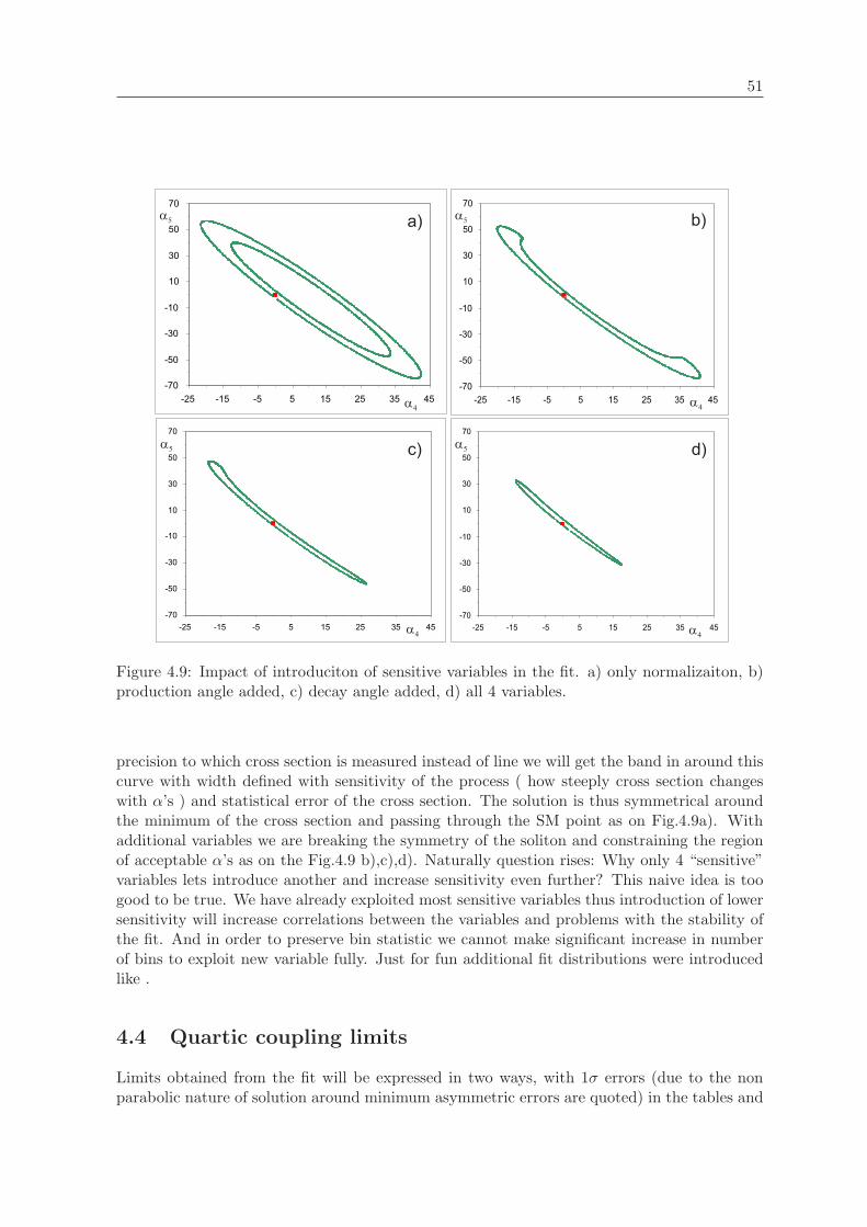
51
Figure 4.9: Impact of introduciton of sensitive variables in the fit. a) only normalizaiton, b)production angle added, c) decay angle added, d) all 4 variables.
precision to which cross section is measured instead of line we will get the band in around thiscurve with width defined with sensitivity of the process ( how steeply cross section changeswith α’s ) and statistical error of the cross section. The solution is thus symmetrical aroundthe minimum of the cross section and passing through the SM point as on Fig.4.9a). Withadditional variables we are breaking the symmetry of the soliton and constraining the regionof acceptable α’s as on the Fig.4.9 b),c),d). Naturally question rises: Why only 4 “sensitive”variables lets introduce another and increase sensitivity even further? This naive idea is toogood to be true. We have already exploited most sensitive variables thus introduction of lowersensitivity will increase correlations between the variables and problems with the stability ofthe fit. And in order to preserve bin statistic we cannot make significant increase in numberof bins to exploit new variable fully. Just for fun additional fit distributions were introducedlike .
4.4 Quartic coupling limits
Limits obtained from the fit will be expressed in two ways, with 1σ errors (due to the nonparabolic nature of solution around minimum asymmetric errors are quoted) in the tables and

52 Chapter 4. Analysis and Results
Table 4.11: Results for all scattering processes in e+e− collisions, assuming isospin conserva-tion.
process α4 α5
e+e− → σ− σ+ σ− σ+ννW+W− -3.97 2.88 -3.11 3.33ννZZ -3.76 3.50 -1.72 1.62e±νW∓Z -3.01 4.31 -3.62 4.57e+e−ZZ -3.63 3.59 - -
Table 4.12: Results for all weak boson scattering processes in e−e− collisions, assuming isospinconservation.
process α4 α5
e−e− → σ− σ+ σ− σ+ννW+W− -8.95 12.44 -22.63 19.23e−νW−Z -6.39 7.66 -6.17 9.93
with the 70% and 95% confidence level contours on the plots, when applicable. Error matricesand correlation coefficients are in appendix.
Electron positron channels
For e+e− channel as already stated we assumed luminosity of 1ab−1 at center of mass energyof 1TeV. Results are summarized in Table.4.11 and in Fig.4.10, for isospin conserving case.In ννW+W− channel there is only dependence to α4 and α5 so this is only possible solution.In case of ννZZ and e±νW∓Z processes dependence is on linear combinations (α4 +α6) and(α5 + α7) and solution is extracted by setting α6 = α7 = 0. For e+e−ZZ channel we havedependence on all couplings in the form (α4 +α5 + 1
2(α6 +α7 +α10)) due to the low number ofselected events no simultaneous extraction of α4 and α5 is possible thus results are extractedfro normalization only in form of α4 setting other couplings to 0.
Electron electron channels
Due to the anti pinch effects luminosity in e−e− collisions is significantly lower (∼ 1/3 ofe+e−). Due to this facts we have taken luminosity that is equivalent to the same runningtime as in e+e− option for the reference one (3050fb−1). Result are summarized in Table.4.12and Fig.4.11. Results for both stated channels are obtained under same conditions as ine+e−. Result for the e−e−ZZ channel is missing since ewen with significant effort significantseparation of the signal was possible.
General conclusion that holds for all considered processes is that form single channel desiredlevel of precision (O(1)) cannot be acheaved (with realistic luminosity) even with additionalassumptions like isospin conservation. Thus we need combination of measurements to enhanceoverall knowledge about quartic couplings and underlying physics.
4.4.1 Combined results
Since we have used likelihood for extraction of sensitivity technically obtaining combined resultfor several processes is technically straight forward. First of all on can consider combination

53
Figure 4.10: Sensitivity limits for weak boson scattering processes at 1TeV. Luminosity of1ab−1 is assumed. 70%CL in full line, 95%CL in dotted.
Figure 4.11: Sensitivity limits for ννW−W− channel and e−−Z on the right. Luminosity of350fb−1 is assumed. 70%CL in full line, 95%CL in dotted
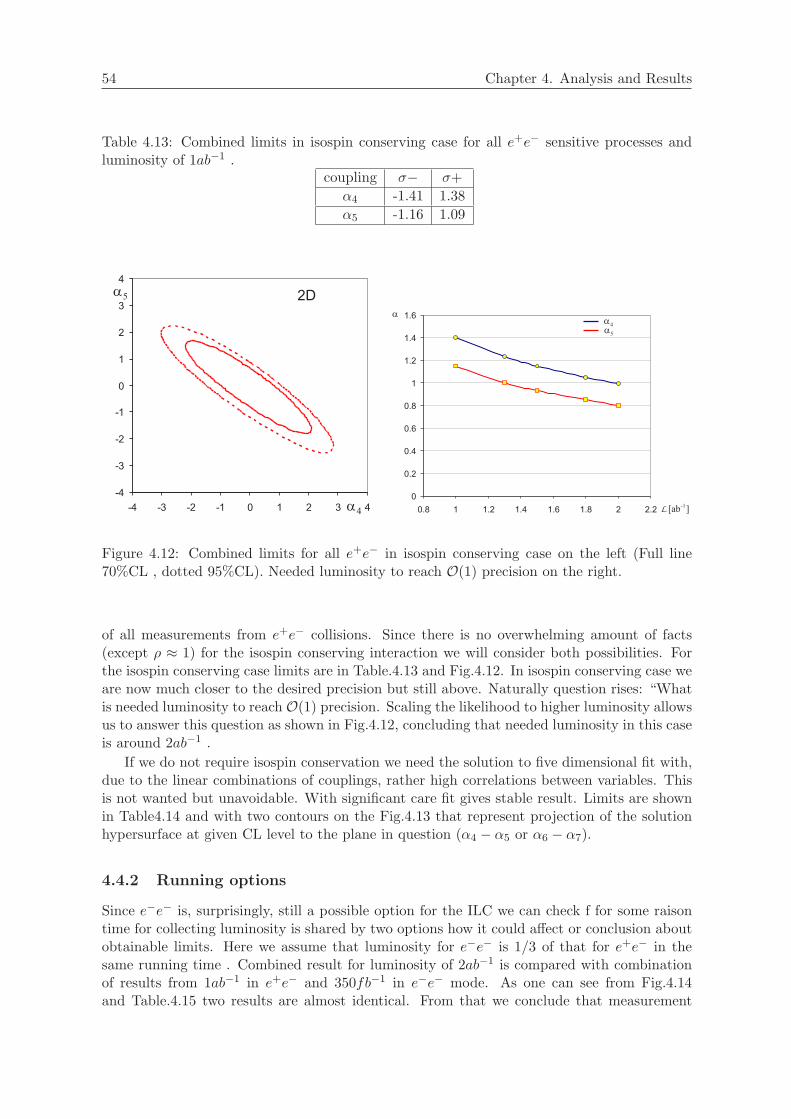
54 Chapter 4. Analysis and Results
Table 4.13: Combined limits in isospin conserving case for all e+e− sensitive processes andluminosity of 1ab−1 .
coupling σ− σ+α4 -1.41 1.38α5 -1.16 1.09
Figure 4.12: Combined limits for all e+e− in isospin conserving case on the left (Full line70%CL , dotted 95%CL). Needed luminosity to reach O(1) precision on the right.
of all measurements from e+e− collisions. Since there is no overwhelming amount of facts(except ρ ≈ 1) for the isospin conserving interaction we will consider both possibilities. Forthe isospin conserving case limits are in Table.4.13 and Fig.4.12. In isospin conserving case weare now much closer to the desired precision but still above. Naturally question rises: “Whatis needed luminosity to reach O(1) precision. Scaling the likelihood to higher luminosity allowsus to answer this question as shown in Fig.4.12, concluding that needed luminosity in this caseis around 2ab−1 .
If we do not require isospin conservation we need the solution to five dimensional fit with,due to the linear combinations of couplings, rather high correlations between variables. Thisis not wanted but unavoidable. With significant care fit gives stable result. Limits are shownin Table4.14 and with two contours on the Fig.4.13 that represent projection of the solutionhypersurface at given CL level to the plane in question (α4 − α5 or α6 − α7).
4.4.2 Running options
Since e−e− is, surprisingly, still a possible option for the ILC we can check f for some raisontime for collecting luminosity is shared by two options how it could affect or conclusion aboutobtainable limits. Here we assume that luminosity for e−e− is 1/3 of that for e+e− in thesame running time . Combined result for luminosity of 2ab−1 is compared with combinationof results from 1ab−1 in e+e− and 350fb−1 in e−e− mode. As one can see from Fig.4.14and Table.4.15 two results are almost identical. From that we conclude that measurement

55
Table 4.14: Combined limits for all e+e− sensitive processes and luminosity of 1ab−1 .coupling σ− σ+α4 -2.70 2.88α5 -2.48 2.34α6 -3.92 5.54α7 -3.20 3.04α10 -5.18 4.53
Figure 4.13: Combine limits for all e+e− processes. Confidence level contour in α4 − α5 plain(a), and in α6 − α7 plain (b). Full line 70%CL , dotted 95%CL.

56 Chapter 4. Analysis and Results
Figure 4.14: Limits in combination of collider running options. In blue only e+e− mode inred combination of e+e− and e−e− measurements. Full line 70%CL limit , dotted 95%CL.
Table 4.15: Comparison of running modes. for 2ab−1 in e+e− collisions and combination of1ab−1 for e+e− channels wiht 350fb−1 in e−e− under assumption of isospin conservation.
e+e− e+e− and e−e−
coupling σ− σ+ σ− σ+α4 -0.99 0.98 -0.87 0.94α5 -0.82 0.78 -0.99 0.84
of quartic couplings does not restrict flexibility of physics program is case of the unexpected.There is a restriction to this flexibility. Part of the running time in the e+e− mode is mustsince only ν that is to say WW → ZZ channel possesses high enough sensitivity to restrictα5 thus running only in e−e− is not desired by this measurement.
4.5 Model dependent limits on new physics
In any measurement the goal is not just to obtain the number but to understand what itmeans. Latest at this step there is a need to drop so far pursued goal of model independenceand to interprete the results in particular scenario of new physics.

57
4.5.1 Combination of measurements
Any new physics scenario will not manifest itself in one and only one physics measurement. Inorder to describe the new phenomena usually several measurements are needed, on the otherhand analysis results often neglect this natural synergy. But physics analysis are often donein such way that it is very difficult to combine their results in natural way eider due to theway results are presented or due to the incompatibility of assumptions and(or) approximationthat were made. As already explained measurement of the quartic couplings comes in laterstage of the ILC operation not only due to the luminosity and center of mass energy neededbut also due to requirements that other chiral couplings of lower order are measured with highprecision. Final word on measurement prospects can be sad after covering all measurementthat are prerequisite to ours, covering the all decay channels of the weak bosons (not onlyhadronic ones as in our case) and all sources of information (analysis based on rescatteringto yet done), nevertheless an attempt to demonstrate this approach was made by combininganalysis results of triple weak boson production (although with different positron polarizationassumption) and weak boson scattering processes together with additional information fromTGC measurement (center of mass energy 800GeV assumed). It is hard to estimate how totalluminosity considered in mentioned analysis corresponds to the one finally available for thephysics program at given energies, thus more precise estimate of available information for theevaluation of physics reach of such measurement can be sad only once such information exists.Possible impact of the inclusion of rescattering effects in the W pair production used for TGCmeasurement is also not considered. Even with these know uncertainties we will proceed ininterpretation of the results keeping in mind that more consistent set of inputs is needed.
4.5.2 Mass limit extraction
We will interprete our results in terms of masses of would be resonances with given quantumnumbers as already introduced in chapter 3. Each would be resonance on the bases of theirLagrangian establishes system of equations:
αi = fi(k1, ..., kj ,M) i ∈ {4, 5, 6, 7, 10} (4.17)
where kj are internal couplings in the resonance Lagrangian, and M is resonant mass. Sinceboth k’s and M are unknown system cannot be solved. Additionally to this there is a relationof the resonance width to it’s mass and couplings:
Γ = F (k1, ..., kj ,M) (4.18)
Addition of this equation dose not change the nature of the system we still have more unknownsthen the equations. At this step we need to make an assumption. Weakest one and moststraight forward is to declare width as “known” parameterizing as a fraction of the mass:
Γ = fwM (4.19)
where fw is coefficient set by hand. With this we have reduced number of unknowns by onemaking it possible to solve, getting :
M = G(fw, αi) (4.20)
mass as a function of alphas, and fraction fw. Since fw is postulated we will express resultsfor different values of fw considering broader and narrower resonances. Limits obtained inprevious chapter for quartic couplings cannot be used directly in this procedure sine alphas

58 Chapter 4. Analysis and Results
0.1 0.2 0.3 0.4 0.516Π2Α5
1.5
2
2.5
3M @TeVD
Figure 4.15: Mass of the scalar resonance as a function of α5 in scalar singlet model, withthe resonance width to mass ratio fσ equal to 1.0 in full line, 0.8 dashed, 0.6 dot-dashed, 0.3dotted line. One sigma limit on the α5 as vertical line on the plot.
should satisfy set of equations 4.17. In general there are two possibilities j < i over constrainedsystem (adding at least one relation of the type αi = gi(~α)) or j = i normal situation, togetherwith possibility fi ≡ 0. In order to extract quartic coupling limits in particular model alphaswere set to zero when applicable and additional relations were exploited when they exist toreduce the number of free alphas to the minimal value. Fitting is then redone and values ofthe couplings used in eq.4.20 were obtained. Fit is done with Minuit as usual but in somecases where we have additional coupling relations already highly correlated system was toomuch even for the most stable minimum search methods. In those cases brute force minimumsearch was performed on the grid in parameter space. All the algebraic computations (leadingto the solution 4.20) were done with Mathematica [60] to prevent human made contributionsto the new physics.
4.6 Mass limit results
4.6.1 Scalar singlet
Isospin conservation
Lets start from the system of equations 3.82 and 3.83. First we will consider isospin conservingcase, hσ = 0, which leads to α7 = α10 = 0. Since α4 = α6 = 0, there is only a dependence onα5 as a free parameter. After the fit, we get σα5 = 0.42 for the symmetric error or −0.452 <α5 < 0.397 for the asymmetric ones at 1σ level. Expressing the width of the resonance as afraction of its width, Γσ = fσMσ, it is possible to solve eq. (3.83) and α5 = g2
σv2
8M2σ
to obtainthe resonance mass as a function of the quartic coupling and this fraction:
Mσ = v
(4πfσ3α5
) 14
(4.21)
In Fig. 4.15, we plot the mass of a scalar singlet resonance as a function of the coupling for agiven width. The vertical line in the plot is the 1σ sensitivity limit. Results are summarizedin the Table.4.6.1

59
fσ = ΓσMσ
1.0 0.8 0.6 0.3Mσ [TeV] 1.55 1.46 1.36 1.15
Table 4.16: Mass reach for the scalar resonance in the SU(2)c conserving case depending ondifferent resonance widths.
0.1 0.2 0.3 0.4 0.5Α5
-0.8
-0.6
-0.4
-0.2
0.2
0.4
Α7
0.1 0.2 0.3 0.4 0.516Π2Α5
1.2
1.4
1.6
1.8M @TeVD
Figure 4.16: On the left, 1σ contour in the α5 − α7 plane. On the right, the dependence ofthe resonance mass on α5 along the contour for fσ = 1 (width equal to the mass) in full, andfσ = 0.8 in dashed and fσ = 0.6 in dot-dashed. Upper and lower lines correspond to thedifferent branches of the solution of α7 = F [α5], respectively.
Isospin violation
If we allow for isospin violation, α4 and α6 are still zero, leaving the three free parameters α5,α7 and α10 for the fit. With only two independent variables, the system of equations (3.82) isover constrained with the additional relation:
α27 = 2α5α10 (4.22)
that should hold exactly.Using this equation it is possible to eliminate one of the couplings from further considera-
tion. We will choose to eliminate α10. Solving the system of equations, it is now possible toexpress the mass as a function of the width, α5 and α7:
Mσ = v
(4πα5fσ
2α25 + (α5 + 2α7)2
) 14
. (4.23)
If we limit ourselves to the case that we vary the couplings only along the 1σ contour in theα5,α7 plane, we end up with the result shown in Fig. 4.16. The lower of the two curves (dashedone) gives a lower boundary to the allowed region for the scalar singlet case. Upper boundaryyou can extract from the maximum of the mass formulae . This gives α7 = −α5 and leads tofunctional dependence of upper boundary as:
Mσ = v
(2πfσα5
) 14
. (4.24)
Now it is possible to fully constrain the region in α5 and M parameter plain. Result is shownin Fig.4.17

60 Chapter 4. Analysis and Results
fσ = ΓσMσ
1.0 0.8 0.6Mσ [TeV] 1.39 1.32 1.23
Table 4.17: Average mass along the contour for the scalar resonance in the isospin breakingcase depending on different resonance widths. Numbers in the table are averaged values alongthe lower limit.
0.1 0.2 0.3 0.4 0.516Π2Α5
1.2
1.4
1.6
1.8
2
2.2M @TeVD
Figure 4.17: Allowed region for scalar singlet resonance with isospin breaking in dependenceon α5 between upper and lower boundary. Ratio of width to mass equal to 1.0 in full, 0.8dashed , 0.6 dot-dashed.

61
0.2 0.4 0.6 0.8 1 1.2 1.416Π2Α6
1.25
1.5
1.75
2
2.25
M @TeVD
Figure 4.18: Dependence of the resonance mass for the charged component on α6 for differ-ent assumed widths (in fπ = Γπ/Mπ = 1.0 in red, 0.8 in green,0.6 in blue, 0.3 in brown,respectively). The red vertical line represents the maximal value of α6 along the 1σ surface.
fπ = ΓπMπ
1.0 0.8 0.6 0.3Mπ0 [TeV] 1.49 1.41 1.31 −Mπ± [TeV] 1.55 1.47 1.37 1.15
Table 4.18: Dependence of the mass reach for scalar triplet resonances on different resonancewidths. For neutral component numbers in the table are average values along the lower limit.
4.6.2 Scalar triplet
Considering system of equations 3.86 and 3.87 we can distinguish two solution branches. (a)In the case of α6 = α7 = α10 = 0 with apparent isospin conservation the solution for Massdependence on couplings reduces to the isospin conserving case for scalar singlet. With nocontribution to the width of charged component.
Mπ0 = v
(4πfπ0
3α5
) 14
(4.25)
(b) If we allow for isospin breaking, only α4 remains zero and we get the constrain:
α27 = 2α5(α6 + α10), (4.26)
which is the generalization of the singlet case. Again we use over constraining to eliminateα10. Solving the remaining system we get:
Mπ± = v
(4πfπ±α6
) 14
(4.27a)
Mπ0 = v
(2πα5fπ0
α25 + (α5 + α7)2
) 14
(4.27b)
with additional condition that α5 and α6 must be positive in order to get real solutions forthe mass.
Results are shown in Table.4.6.2.
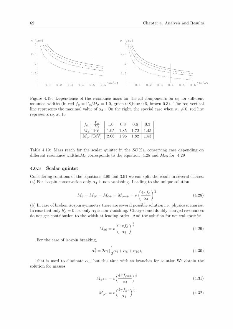
62 Chapter 4. Analysis and Results
0.1 0.2 0.3 0.4 0.5 0.616Π2Α4
1.5
2
2.5
3M @TeVD
0.1 0.2 0.3 0.4 0.5 0.616Π2Α5
1.5
2
2.5
3M @TeVD
Figure 4.19: Dependence of the resonance mass for the all components on α4 for differentassumed widths (in red fφ = Γφ/Mσ = 1.0, green 0.8,blue 0.6, brown 0.3). The red verticalline represents the maximal value of α4 . On the right, the special case when α5 6= 0, red linerepresents α5 at 1σ
fφ = Γφ
Mφ1.0 0.8 0.6 0.3
Mφ [TeV] 1.95 1.85 1.72 1.45Mφ0 [TeV] 2.06 1.96 1.82 1.53
Table 4.19: Mass reach for the scalar quintet in the SU(2)c conserving case depending ondifferent resonance widths.Mφ corresponds to the equation 4.28 and Mφ0 for 4.29
4.6.3 Scalar quintet
Considering solutions of the equations 3.90 and 3.91 we can split the result in several classes:(a) For isospin conservation only α4 is non-vanishing. Leading to the unique solution
Mφ = Mφ0 = Mφ+ = Mφ++ = v
(4πfφα4
) 14
(4.28)
(b) In case of broken isospin symmetry there are several possible solution i.e. physics scenarios.In case that only h′φ = 0 i.e. only α5 is non-vanishing. Charged and doubly charged resonancesdo not get contribution to the width at leading order. And the solution for neutral state is:
Mφ0 = v
(2πfφα5
) 14
(4.29)
For the case of isospin breaking,
α27 = 2α5(
12α4 + α6 + α10), (4.30)
that is used to eliminate α10 but this time with to branches for solution.We obtain thesolution for masses
Mφ±± = v(4πfφ±±
α4
) 14 (4.31)
Mφ± = v(4πfφ±
α4
) 14 (4.32)

63
Mφ0 = v( 12πα5fφ0
(√α4α5 − 2α5)2 + 2(α5 + α7)
) 14 (4.33)
For the doubly charged component situation is clear if gφ is not zero there is a contributionto it, and we can extract the mass limit in the usual way.
For single charged component there is a special situation when α4 = −α6 when we haveno contribution to the width of this component but still contributions to the width of neutraland doubly charged ones. Relation between couplings reduces to
α27 = 2α5(−1
2α4 + α10) & α6 = −α4 (4.34)
And we have expressions for the mass
Mφ++ = v
(4πfφ++
α4
) 14
(4.35)
Mφ0 = v
(12πα5fφ0
2(α5 + α7)2 + α5(√α4 − 2
√α5)2
) 14
(4.36)
For special case a) lower limits are the same only difference is that there is no upper limitfor neutral case since there is a singular direction of mass equation when denominator is zerobut α5 is still nonzero. this can be seen on the plot ( maybe to drop this plot at all I’ll redoit in nicer way anyhow)
special case b) .. hφ = kφ = 0 leads to α6 = α10 = 0 contributions to the chargedcomponents are the same.
Mφ++ = Mφ+ = v
(4πfφ++
α4
) 14
(4.37)
Mφ0 = v
(4πα4fφ0
α42 + 2α7
2
) 14
(4.38)
with the relation between couplings reduced to:
α72 = α5α4 (4.39)
c) general case
fφ = Γφ
Mφ1.0 0.8 0.6 0.3
Mφ [TeV] 1.95 1.85 1.72 1.45Mφ0 [TeV] 1.77 1.67 1.55 1.31
Table 4.20: Mass reach for the scalar quintet special case b) depending on different resonancewidths.Mφ corresponds to the equation 4.37 and Mφ0 for 4.38 as an average over lower limit

64 Chapter 4. Analysis and Results
0.1 0.2 0.3 0.4 0.5 0.616Π2Α4
1.5
2
2.5
3M @TeVD
0.1 0.2 0.3 0.4 0.5 0.616Π2Α5
1.5
2
2.5
3M @TeVD
Figure 4.20: Dependence of the resonance mass for special case b) on α4 for different assumedwidths (in red fφ = Γφ/Mσ = 1.0, green 0.8,blue 0.6, brown 0.3). The red vertical linerepresents the maximal value of α4 . On the left dependence for charged members,on the leftfor neutral
0.1 0.2 0.3 0.4 0.516Π2Α5
1.2
1.4
1.6
1.8
2M @TeVD
0.1 0.2 0.3 0.4 0.516Π2Α4
1.25
1.5
1.75
2
2.25
M @TeVD
Figure 4.21: from left to right mass dependence in most general case for neutral, charged anddoubly charged component of multiplet
fφ = Γφ
Mφ1.0 0.8 0.6 0.3
Mφ±± [TeV] 1.95 1.85 1.72 1.45Mφ± [TeV] 1.64 1.55 1.44 1.21Mφ0 [TeV] 1.55 1.46 1.35 1.14
Table 4.21: Mass reach for the scalar quintet in most general case.Mφ0 and Mφ± are averagesover lower limit.

65
0.5 1 1.5 2 2.516Π2Α4
1.5
2
2.5
3
M @TeVD
Figure 4.22: Dependence of Mass of vector resonance on α4 for different assumed widths (infπ = Γπ/Mπ = 1.0 in red, 0.8 in blue, 0.3 in brown, respectively), under condition lω = 0
fω = ΓωMω
1.0 0.8 0.6 0.3Mω [TeV] 1.74 1.65 1.53 1.29
Table 4.22: Mass for vector resonance case l=0,for different assumed widths (in fπ = Γω/Mω =1.0 blue 0.8,green 0.6, brown 0.3).
4.6.4 Vector singlet
For vector singlet isospin breaking has to be involved. First we find the solution from thesystem of equation for quartic couplings and additional λ type couplings contributing to thesame order as in (eq.3.92 ). Ignoring the parameter kω since it has no physical meaning interms of the resonance mass and width, at least to the order considered. Relation betweenthe couplings are as:
α1 = α2 = α4 = α7 = −α5 = −α6 = −α8 = −α9 (4.40)
leaving only one free coupling for which we chose α4. Solution for the mass then is:
Mω = v
(96πfω − lω
2
8α4
) 14
(4.41)
For the limit extraction we use simplifying assumption lω = 0 that reduces solution to:
Mω = v
(12πfωα4
) 14
(4.42)
Now we have two free parameters one can be determined from measurement of quarticcouplings α4 but for the second fω we need additional measurement. Such measurement ismeasurement of triple couplings as is [73] or [74]. We use result [73] to construct the χ2 forthe ∆gZ1 ,∆kZ and λZ and use consistent set of numbers at 1σ level. Results for this case areshown in Fig. 4.22 and table 4.6.4.
Now we introduce triple couplings into the solution, but if we want to be consistent onecannot allow cosines and sines of the mixing angles to go above 1. From this one gets naturalupper constrain on the mass. Since only lω is contributing to the width of resonance it’ssufficient to solve M as a function of λz, α4, fω. In the solution λz comes only in squares and it’s

66 Chapter 4. Analysis and Results
0.5 1 1.5 2 2.516Π2Α4
1.5
2
2.5
3
3.5
4
M @TeVD
0.5 1 1.5 2 2.516Π2Α4
1.5
2
2.5
3
3.5
4
M @TeVD
Figure 4.23: Dependence of Mass of vector resonance on α4 for different assumed width equalto the mass on the left and 0.3 of the mass on the right.Red curve is upper limit.Blue one isfor maximal value of λz and brown one for λz = 0 that coincides with discussed case lω = 0
0.02 0.04 0.06 0.08 0.116Π2Α4
2
3
4
5
6
7M @TeVD
Figure 4.24: Dependence of Mass of vector resonance on α4 for different assumed width equalto the mass. Red curve represents constrain coming from β1
thus not sensitive to the sign, and using results from [73] we obtain the range 0 < λz < 0.00033.If we plot now two extreme cases for λz we get.
If I do not use the correction to the cw and sw there is no influence on the result since λzis so small. The result is same as for l=0. If we use the limit α4 = 2.36 and not the cw=1curve averages over lower curve change a bit. If you argue that lower curve still takes intoaccount β1 then forget all and use only consideration with l=0.
4.6.5 Vector triplet
We will consider solutions of equations 3.94, 3.95 and 3.96. For simplicity we assume thatthere is no mass splitting between the neutral and charged state of the resonance. As for thesinglet case parameters kρ,k′ρ and k′′ρ are ignored, as well as the coefficients of the magnetic
fω = ΓωMω
1.0 0.8 0.6 0.3Mω [TeV] 2.22 2.10 1.95 1.63
Table 4.23: Mass limit for vector resonance. Values in the table are average values along thelower limit in the range 0 till 2.36
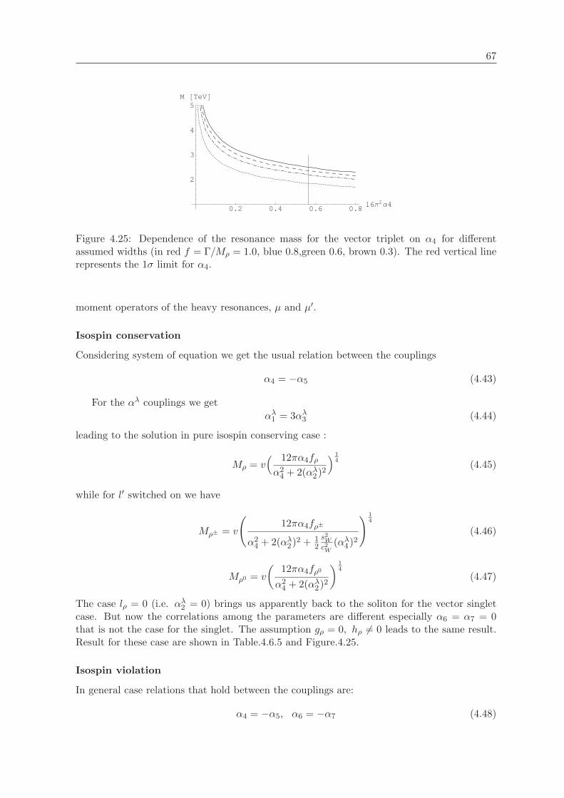
67
0.2 0.4 0.6 0.816Π2Α4
2
3
4
5M @TeVD
Figure 4.25: Dependence of the resonance mass for the vector triplet on α4 for differentassumed widths (in red f = Γ/Mρ = 1.0, blue 0.8,green 0.6, brown 0.3). The red vertical linerepresents the 1σ limit for α4.
moment operators of the heavy resonances, µ and µ′.
Isospin conservation
Considering system of equation we get the usual relation between the couplings
α4 = −α5 (4.43)
For the αλ couplings we getαλ1 = 3αλ3 (4.44)
leading to the solution in pure isospin conserving case :
Mρ = v( 12πα4fρ
α24 + 2(αλ2)2
) 14 (4.45)
while for l′ switched on we have
Mρ± = v
(12πα4fρ±
α24 + 2(αλ2)2 + 1
2s2Wc2W
(αλ4)2
) 14
(4.46)
Mρ0 = v
(12πα4fρ0
α24 + 2(αλ2)2
) 14
(4.47)
The case lρ = 0 (i.e. αλ2 = 0) brings us apparently back to the soliton for the vector singletcase. But now the correlations among the parameters are different especially α6 = α7 = 0that is not the case for the singlet. The assumption gρ = 0, hρ 6= 0 leads to the same result.Result for these case are shown in Table.4.6.5 and Figure.4.25.
Isospin violation
In general case relations that hold between the couplings are:
α4 = −α5, α6 = −α7 (4.48)
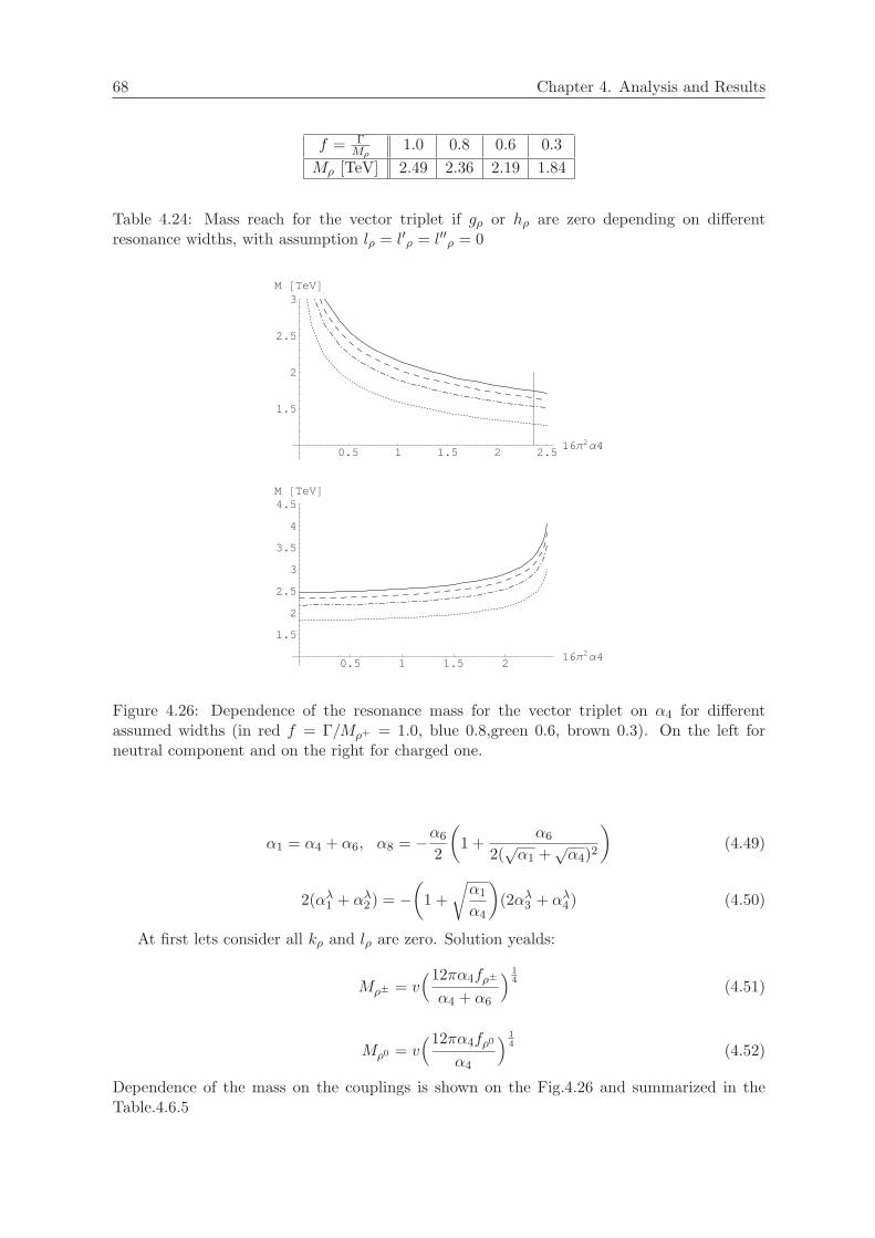
68 Chapter 4. Analysis and Results
f = ΓMρ
1.0 0.8 0.6 0.3Mρ [TeV] 2.49 2.36 2.19 1.84
Table 4.24: Mass reach for the vector triplet if gρ or hρ are zero depending on differentresonance widths, with assumption lρ = l′ρ = l′′ρ = 0
0.5 1 1.5 2 2.516Π2Α4
1.5
2
2.5
3M @TeVD
0.5 1 1.5 216Π2Α4
1.5
2
2.5
3
3.5
4
4.5M @TeVD
Figure 4.26: Dependence of the resonance mass for the vector triplet on α4 for differentassumed widths (in red f = Γ/Mρ+ = 1.0, blue 0.8,green 0.6, brown 0.3). On the left forneutral component and on the right for charged one.
α1 = α4 + α6, α8 = −α6
2
(1 +
α6
2(√α1 +
√α4)2
)(4.49)
2(αλ1 + αλ2) = −(
1 +√α1
α4
)(2αλ3 + αλ4) (4.50)
At first lets consider all kρ and lρ are zero. Solution yealds:
Mρ± = v(12πα4fρ±
α4 + α6
) 14 (4.51)
Mρ0 = v(12πα4fρ0
α4
) 14 (4.52)
Dependence of the mass on the couplings is shown on the Fig.4.26 and summarized in theTable.4.6.5

69
f = ΓMρ
1.0 0.8 0.6 0.3Mρ± [TeV] 2.67 2.53 2.35 1.98Mρ0 [TeV] 1.74 1.65 1.53 1.29
Table 4.25: Mass reach for the vector triplet with assumption lρ = l′ρ = l′′ρ = 0.Values forcharged component are averaged over lower limit
0.5 1 1.5 216Π2Α4
2
3
4
5
6M @TeVD
0.5 1 1.5 216Π2Α4
1.5
2
2.5
3
3.5
4M @TeVD
Figure 4.27: Dependence of the resonance mass for the vector triplet on α4 for differentassumed widths (in red f = Γ/Mρ+ = 1.0, blue 0.8,green 0.6, brown 0.3) for g = −h case. Onthe left for charged and on the right for neutral one.
There is a special case for the solution when gρ = −hρ, relation between the couplingsimplify to:
α1 =13α 2
= −α3 =19α 4
= −18α 6
=12α 9
(4.53)
this leads to the mass solutions in the form:
Mρ± = v
(108πfρ±α4
) 14
(4.54)
Mρ0 = v
(12πfρ0α4
) 14
(4.55)
with results presented in Fig.4.27 and Table.4.6.5.Still assuming gρ = −hρ we can now allow non-zero values for lρ and l′ρ. As in vector singlet
case we need additional measurements in order to solve the system. Using results for λZ andλγ form [73] assuming l′′ρ = 0 we have solvable system. Constructing the χ2 distribution forthe triple couplings and requesting that variables are connected with condition χ2 = χ2
min + 1can solve for the masses although only numerically due to the polynomial equation of higherorder. Results are in the Table.4.6.5 and Fig.4.28 and Fig.4.29. If we allow µ 6= µ′ 6= 0 this
f = ΓMρ
1.0 0.8 0.6 0.3Mρ± [TeV] 3.09 2.92 2.72 2.29Mρ0 [TeV] 1.78 1.69 1.57 1.32
Table 4.26: Mass reach for the vector triplet with assumption g = −h.

70 Chapter 4. Analysis and Results
0.5 1 1.5 216Π2Α4
2
3
4
5
6M @TeVD
0.5 1 1.5 216Π2Α4
2
3
4
5
6M @TeVD
0.5 1 1.5 216p2a4
1.5
2
2.5
3
3.5
4
M @TeVD
0.5 1 1.5 216p2a4
1.5
2
2.5
3
3.5
4
M @TeVD
Figure 4.28: Dependence of the resonance mass for charged component of the vector tripleton α4 for different assumed widths (f=1 on the left and f=0.3 on the right) for gρ = −hρ case.Full line represent the case when lρ = l′ρ = l′′ρ = 0 , and the dashed one minimal value whenwe allow lρ 6= l′ρ 6= 0. The grey shaded area becomes allowed if µρ, µ′ρ 6= 0.
f = ΓMρ
1.0 0.8 0.6 0.3Mρ± [TeV] 2.91 2.75 2.56 2.16Mρ0 [TeV] 1.84 1.79 1.66 1.40
Table 4.27: Mass reach for the vector triplet with assumption g = −h with lρ 6= l′ρ 6= 0.Valuesin the table are average values along the lower limit
leads to 10% reduction in the lower limit but without putting any constrain on to the valuesof µ.
4.6.6 Tensor singlet
Considering system of equations eq.3.97 and eq.3.98 we have following possible solutions:
0.5 1 1.5 216Π2Α4
1.5
2
2.5
3
3.5
4M @TeVD
0.5 1 1.5 216Π2Α4
1.5
2
2.5
3
3.5
4M @TeVD
0.5 1 1.5 216Π2Α4
1.5
2
2.5
3
3.5
4M @TeVD
0.5 1 1.5 216Π2Α4
1.5
2
2.5
3
3.5
4M @TeVD
Figure 4.29: Dependence of the resonance mass for neutral component of the vector triplet onα4 for different assumed widths (f=1 on the left and f=0.3 on the right) for gρ = −hρ case.Full line represent the case when lρ = l′ρ = l′′ρ = 0 , and dashed one minimal value when weallow lρ 6= l′ρ 6= 0. The grey shaded area becomes allowed if µρ, µ′ρ 6= 0

71
f = ΓMρ
1.0 0.8 0.6 0.3Mρ± [TeV] 2.54 2.41 2.34 1.88Mρ0 [TeV] 1.71 1.62 1.51 1.27
Table 4.28: Mass reach for the vector triplet with assumption g = −h with lρ 6= l′ρ 6= 0 whenµ 6= µ′ 6= 0. Values in the table are average values along the lower limit
0.2 0.4 0.6 0.8 116Π2Α4
2
3
4
5M @TeVD
Figure 4.30: Dependence of the resonance mass for the tensor singlet case on α4 for differentassumed widths (full line f = Γ/M = 1.0, dashed 0.8, dot-dashed 0.6, dotted 0.3).
Isospin conservation
For this case α4 and α5 are non-zero but related with:
α5 = −14α4 (4.56)
Choosing α4 as fit variable we get α4 = 0.64369 for parabolic error and −0.65404 < α4 <0.62154 for asymmetric errors at 1σ level. Mass dependence on the coupling is then given by:
M = v
(40πfα4
) 14
(4.57)
Results for this case are shown on the Fig.4.30 and in Table.4.6.6.
Isospin breaking
In this case α6, α7andα10 are also nonzero but with constrains:
α4 = −4α5 & 2α10α5 = −3α72 & α6 = −4α7 (4.58)
f = ΓM 1.0 0.8 0.6 0.3
M [TeV] 3.29 3.11 2.89 2.43
Table 4.29: Mass reach for the tensor singlet in the SU(2)c conserving case depending ondifferent resonance widths.
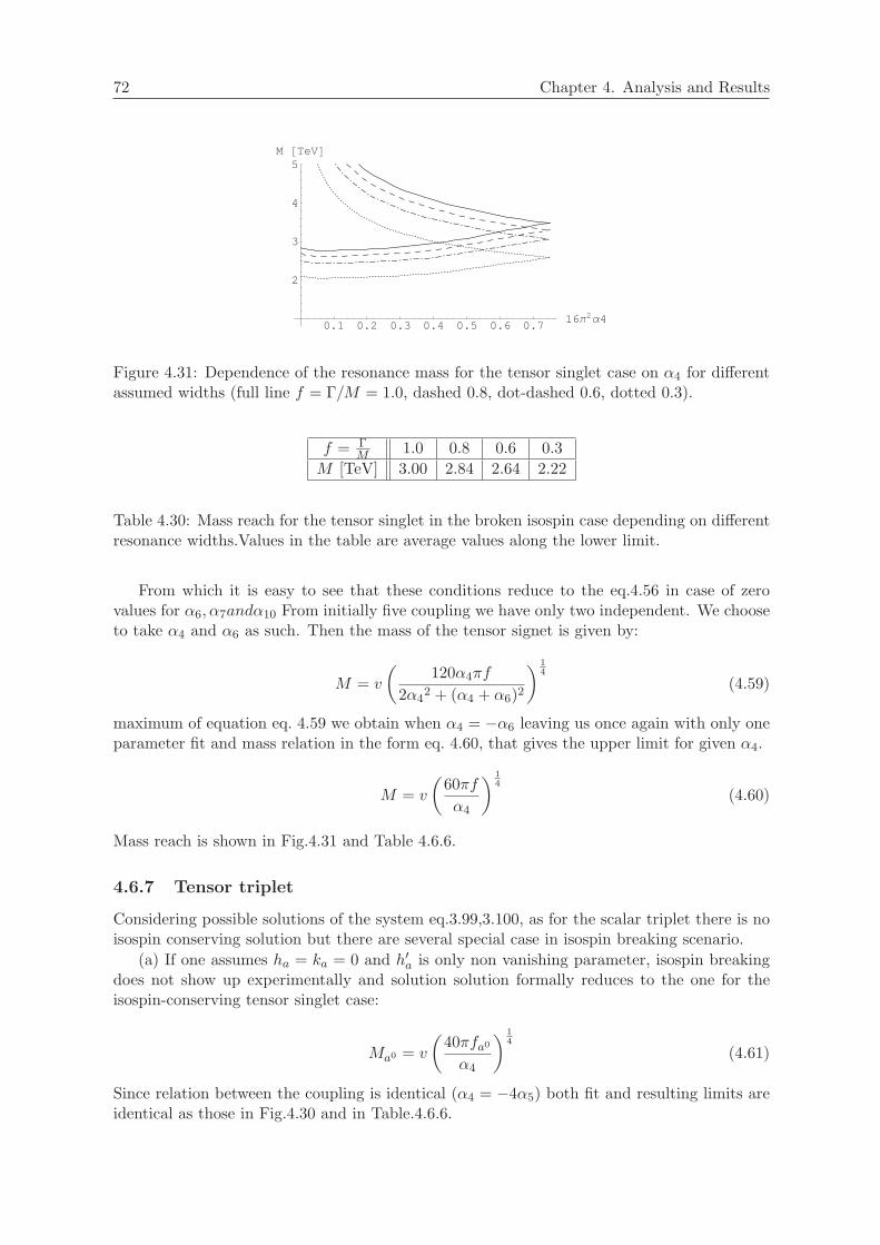
72 Chapter 4. Analysis and Results
0.1 0.2 0.3 0.4 0.5 0.6 0.716Π2Α4
2
3
4
5M @TeVD
Figure 4.31: Dependence of the resonance mass for the tensor singlet case on α4 for differentassumed widths (full line f = Γ/M = 1.0, dashed 0.8, dot-dashed 0.6, dotted 0.3).
f = ΓM 1.0 0.8 0.6 0.3
M [TeV] 3.00 2.84 2.64 2.22
Table 4.30: Mass reach for the tensor singlet in the broken isospin case depending on differentresonance widths.Values in the table are average values along the lower limit.
From which it is easy to see that these conditions reduce to the eq.4.56 in case of zerovalues for α6, α7andα10 From initially five coupling we have only two independent. We chooseto take α4 and α6 as such. Then the mass of the tensor signet is given by:
M = v
(120α4πf
2α42 + (α4 + α6)2
) 14
(4.59)
maximum of equation eq. 4.59 we obtain when α4 = −α6 leaving us once again with only oneparameter fit and mass relation in the form eq. 4.60, that gives the upper limit for given α4.
M = v
(60πfα4
) 14
(4.60)
Mass reach is shown in Fig.4.31 and Table 4.6.6.
4.6.7 Tensor triplet
Considering possible solutions of the system eq.3.99,3.100, as for the scalar triplet there is noisospin conserving solution but there are several special case in isospin breaking scenario.
(a) If one assumes ha = ka = 0 and h′a is only non vanishing parameter, isospin breakingdoes not show up experimentally and solution solution formally reduces to the one for theisospin-conserving tensor singlet case:
Ma0 = v
(40πfa0
α4
) 14
(4.61)
Since relation between the coupling is identical (α4 = −4α5) both fit and resulting limits areidentical as those in Fig.4.30 and in Table.4.6.6.

73
fa = ΓaMa
1.0 0.8 0.6 0.3Ma0 [TeV] 3.01 2.85 2.65 2.23Ma± [TeV] 3.48 3.29 3.06 2.57
Table 4.31: Dependence of the mass reach for tensor triplet resonances on different resonancewidths. For neutral component numbers in the table are average values along the lower limit.
(b) In most general situation with all considered coupling non vanishing we get followingconstrains:
α4 = −4α5 && (2α6 − α7)2 =92α4(α6 + 4α7 + 3α10) (4.62)
that are used to eliminate α5 and α10 from the system giving the mass solutions:
Ma± = v
(60πfa±α4
) 14
(4.63a)
Ma0 = v
(9720πα4fa0
162α24 + (9α4 + 8α6 − 4α7)2
) 14
(4.63b)
In this case we have three independent couplings thus we have 1σ volume. For the chargedcomponent Situation was rather simple after the fit knowing the error matrix we construct χ2
that is depending on three variables α4, α6 and α7. Condition that up value of χ2 correspondsto the 1σ limit reduces number of free variables to 2. This allow us to plot Mass dependence onthe single variable since for a given α4 within the fit limits one calculates value of α7 subtitlesthem in mass equation and plots. For the neutral component case this in not enough to picktriplet of points thus additional condition 9α4 +8α6− 4α7 is introduces. Fixing third variablealong this surface that guarantees the maximum of eq.4.63a we can do the explained thickagain and plot mass dependence on one coupling only. Note that in this case solution for theneutral state becomes:
Ma0 = v(60πfa0
α4
) 14 (4.64)
Minimum within the 1σ volume we get on the surface of 9α4 + 8α6 − 4α7 = 0 when thesolution for the neutral component becomes same as for the charged component.This conditionis equivalent to the h′(h′+h+2k) = 0 , and h′a cannot be zero since otherwise we do not haveany solution at all. Results are shown in Fig.4.32 Fig.4.33 and in table 4.6.7.
4.6.8 Tensor quintet
Isospin conservation
From system of equations (eq.3.101 and eq.3.102) after checking for nontrivial solution whereα4 and α5 are non-zero we get the following set of constrains
gt 6= 0 , ht = kt = h′t = 0 (4.65)
h′t 6= 0 , gt = kt = ht = 0 (4.66)

74 Chapter 4. Analysis and Results
-1 -0.75 -0.5 -0.25 0.25 0.516Π2Α6
1.5
2
2.5
3
3.5
4M @TeVD
Figure 4.32: Dependence of the resonance mass for the charged component of triplet on α4
for different assumed widths f = Γ/M = 1.0 full, e 0.8 dashed, 0.6 dot-dashed, 0.3 dotted).Vertical line represents the 1σ limit for α4.
0.1 0.2 0.3 0.4 0.5 0.6 0.716Π2Α4
2
3
4
5
M @TeVD
Figure 4.33: Dependence of the resonance mass for the neutral component of triplet on α4 fordifferent assumed widths ( f = Γ/M = 1.0 full, e 0.8 dashed, 0.6 dot-dashed, 0.3 dotted).
h′t = ht = 0 , gt = −2kt (4.67)
h′t = 0 , gt = kt = −12ht (4.68)
h′t = 0 , gt = 2kt = −12ht (4.69)
In all possible combinations relation α5 = 2α4 holds, except for the case from eq.4.66 whereit is α5 = −1
4α4. This leads to two distinct solutions (a) First one is strict isospin conservation(eq.4.65). Solving for mass yealds
Mt = v(
30πft
α4
) 14 (4.70)
After elimination of α5 and fit we obtain α4 = 0.16116 as a parabolic error and −0.17387 <α4 < 0.15134 as asymmetric once at 1σ. Results are shown in Fig.4.34 and Table.4.32. Sameresult we get for cases where h′t = 0 that are experimentally unobservable as isospin breakingcases.

75
0.1 0.2 0.3 0.416Π2Α4
3
4
5
6
7M @TeVD
0.2 0.4 0.6 0.8 116Π2Α4
3
4
5
6
7M @TeVD
Figure 4.34: Dependence of the resonance mass for the tensor quintet b) case on α4 for differentassumed widths (in red f = Γ/Mt = 1.0, blue 0.8,green 0.6, brown 0.3). The red vertical linerepresents the 1σ limit for α4.
f = ΓMt
1.0 0.8 0.6 0.3Mt [TeV] 4.30 4.06 3.78 3.18
Table 4.32: Mass reach for the tensor singlet in the SU(2)c conserving case b) depending ondifferent resonance widths.
Isospin breaking
a) gt = kt = ht = 0 hp = free in this case we have contribution only to the width of neutralmember.Relation between the couplings is α5 = −1
4α4. Mass dependence is
Mt0 = v(
60πft
α4
) 14 (4.71)
c) special case ht = kt = 0 leads to
α6 = −4α7 81α72 = 2α4
2 + 7α4α5 − 4α52 (4.72)
Mtc = v(
270πftc
α4+4α5
) 14 (4.73)
Mt0 = v(
270πft0
5α4+2α5
) 14 (4.74)
(d) In completely general case all couplings are non-zero and the constraint equation is
(2α6 − α7)2 = (2α4 − α5)(α4 + 4α5 + 2α6 + 8α7 + 6α10) (4.75)
f = ΓMt0
1.0 0.8 0.6 0.3Mt0 [TeV] 4.65 4.40 4.10 3.44
Table 4.33: Mass reach for the tensor singlet in the SU(2)c conserving case a) depending ondifferent resonance widths.
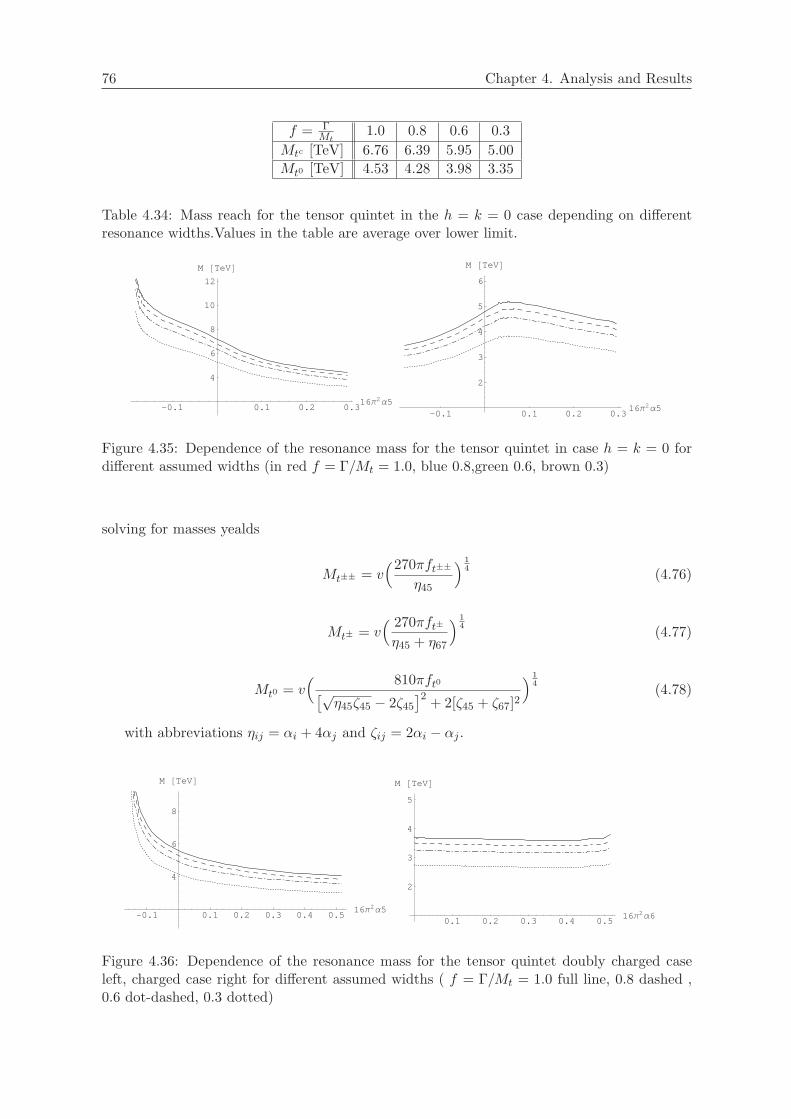
76 Chapter 4. Analysis and Results
f = ΓMt
1.0 0.8 0.6 0.3Mtc [TeV] 6.76 6.39 5.95 5.00Mt0 [TeV] 4.53 4.28 3.98 3.35
Table 4.34: Mass reach for the tensor quintet in the h = k = 0 case depending on differentresonance widths.Values in the table are average over lower limit.
-0.1 0.1 0.2 0.316Π2Α5
4
6
8
10
12
M @TeVD
-0.1 0.1 0.2 0.316Π2Α5
2
3
4
5
6
M @TeVD
Figure 4.35: Dependence of the resonance mass for the tensor quintet in case h = k = 0 fordifferent assumed widths (in red f = Γ/Mt = 1.0, blue 0.8,green 0.6, brown 0.3)
solving for masses yealds
Mt±± = v(270πft±±
η45
) 14 (4.76)
Mt± = v( 270πft±η45 + η67
) 14 (4.77)
Mt0 = v( 810πft0[√
η45ζ45 − 2ζ45
]2 + 2[ζ45 + ζ67]2
) 14 (4.78)
with abbreviations ηij = αi + 4αj and ζij = 2αi − αj .
-0.1 0.1 0.2 0.3 0.4 0.516Π2Α5
4
6
8
M @TeVD
0.1 0.2 0.3 0.4 0.516Π2Α6
2
3
4
5
M @TeVD
Figure 4.36: Dependence of the resonance mass for the tensor quintet doubly charged caseleft, charged case right for different assumed widths ( f = Γ/Mt = 1.0 full line, 0.8 dashed ,0.6 dot-dashed, 0.3 dotted)

77
0.1 0.2 0.3 0.4 0.516Π2Α6
2
3
4
5
6
7
8
M @TeVD
Figure 4.37: Dependence of the resonance mass for the tensor quintet neutral case for differentassumed widths ( f = Γ/Mt = 1.0 full line, 0.8 dashed , 0.6 dot-dashed, 0.3 dotted)
f = ΓMt
1.0 0.8 0.6 0.3Mt±± [TeV] 5.17(4.06) 4.89(3.84) 4.55(3.57) 3.83(3.00)Mt± [TeV] 3.64 3.44 3.20 2.69Mt0 [TeV] 5.84 5.52 5.14 4.32
Table 4.35: Mass reach for the tensor quintet in the full case depending on different resonancewidths.Values in the table are average over lower limit.In brackets minimal value along thelower limit
4.7 Summary
At an ILC with high energy (1TeV) and luminosity (1ab−1) and possibility for both electronand positron polarization, precise measurement of weak boson interactions will be feasible.In Table.4.7 and Table.4.7 results are combined for all spin and isospin channels. Table.4.7assumes SU(2)c conservation, so the ∆ρ parameter automatically vanishes. In this case onlychannels with I+J even couple to weak boson pairs. Table.4.7 shows results without thisconstrain. In each case, a single resonance with maximal coupling (i.e. Γ = M) was assumedto be present. In a real situation particular structure of the parameter dependence can beused to disentangle multiple resonances. Amount of information that can possibly be gainedon top of the analysis of fermionic couplings, or otherwise if such couplings are small or absent.In this case only operator that scales with 1/M2 corresponds to the ρ parameter associatedto custodial-SU(2) violation. Apart from that, all 1/M2 effects in bosonic interactions canbe absorbed into unobservable redefinition of the SM parameters. All shifts due to heavyresonances in oblique corrections, triple gauge couplings and quartic couplings scale with1/M4. Taking these consideration into account, We find limits for the sensitivity of theILC in the 1 to 3TeV range, where the best reach corresponds to the highest spin/isospinchannel.These limits are not as striking as possible limits from contact interactions, but theyagree well with the expected direct search limits for resonances at LHC. Performing globalfits of all electroweak parameters, analogous to LEP analysis, and combining data from bothexperiments well be important for disentangling the contributions. Significant knowledgeabout the mechanism of electroweak symmetry breaking can thus be gained even in the casewhen no new particle content of the theory is discovered.

Spin I=0 I=1 I=20 1.55 - 1.951 - 2.49 -2 3.29 - 4.30
Table 4.36: Accessible scale in TeV for all possible spin/isospin channels. Custodial SU(2)symmetry is assumed to hold.
Spin I=0 I=1 I=20 1.39 1.55 1.951 1.74 2.67 -2 3.00 3.01 5.84
Table 4.37: Accessible scale in TeV for all possible spin/isospin channels. Custodial SU(2)symmetry is assumed to hold.
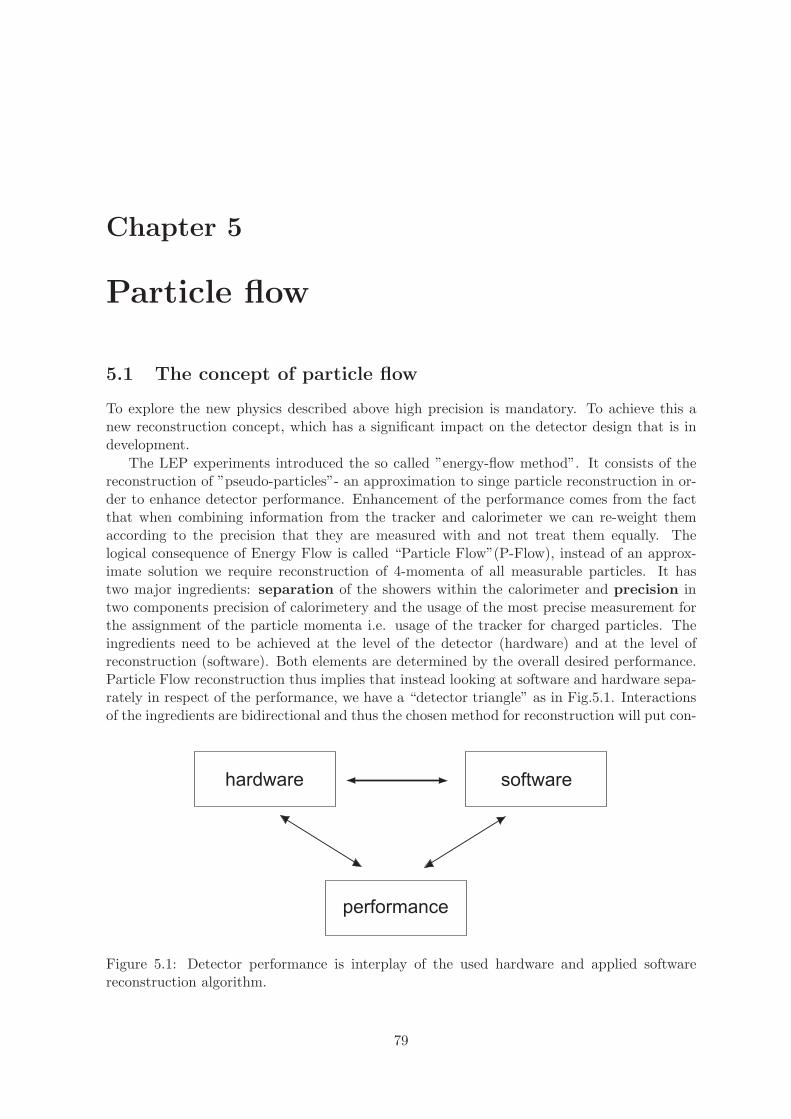
Chapter 5
Particle flow
5.1 The concept of particle flow
To explore the new physics described above high precision is mandatory. To achieve this anew reconstruction concept, which has a significant impact on the detector design that is indevelopment.
The LEP experiments introduced the so called ”energy-flow method”. It consists of thereconstruction of ”pseudo-particles”- an approximation to singe particle reconstruction in or-der to enhance detector performance. Enhancement of the performance comes from the factthat when combining information from the tracker and calorimeter we can re-weight themaccording to the precision that they are measured with and not treat them equally. Thelogical consequence of Energy Flow is called “Particle Flow”(P-Flow), instead of an approx-imate solution we require reconstruction of 4-momenta of all measurable particles. It hastwo major ingredients: separation of the showers within the calorimeter and precision intwo components precision of calorimetery and the usage of the most precise measurement forthe assignment of the particle momenta i.e. usage of the tracker for charged particles. Theingredients need to be achieved at the level of the detector (hardware) and at the level ofreconstruction (software). Both elements are determined by the overall desired performance.Particle Flow reconstruction thus implies that instead looking at software and hardware sepa-rately in respect of the performance, we have a “detector triangle” as in Fig.5.1. Interactionsof the ingredients are bidirectional and thus the chosen method for reconstruction will put con-
Figure 5.1: Detector performance is interplay of the used hardware and applied softwarereconstruction algorithm.
79

80 Chapter 5. Particle flow
Figure 5.2: Dependence of the absolute event energy resolution for different jet energy param-eterization in comparison with calorimeter sum. Points for the calorimtere sum width are fordifferent processis and the conector line is just to guide the eye.
strains on the hardware parameters and different hardware parameters will impact methods tobe chosen in reconstruction governed by the performance goal that is set. In order to acheiveoptimal design of the detector components it is mandatory to develop an understanding of allcontributions to the overall performance and to make their proper factorization. Jet energyresolution is usually expressed in the form:
∆EE
=a√E
(5.1)
with the performance goal a=30%. Recently a parameterization is introduced [20] in the form:
∆EE
= b (5.2)
where b ∼ 3− 4% driven with idea to have reconstructed width comparable with the naturalwidth of the weak bosons, althoe it is not equivalent to the one from eq.5.1. As we can see inFig.5.2 approximate equivalence of the parameterizations exists only around 90GeV. The newparameterization (with b=3%) crosses the performance of the calorimeter sum in the LDCdetector [78] at ∼ 270GeV making concept of the Particle Flow obsolete. Not to mention thatat ∼ 400GeV is equivalent to the best LEP performance of 60%
√E so there cannot be any
room for “the superior performance of ILC Detector”, and we should remind ourself that such“performance” would require some 40% more luminosity for the the precision measurementfor various processes [79, 80, 81, 82, 83] in comparison with performance goal of 30%
√E. For
this reason we will continue to use eq.5.1 in the following.

81
Table 5.1: Comparison of the calorimeter performance of the LEP and LDC detector in terms
of resolution,segmentation and Perfect Particle Flow (PPF) performance.
ALEPH DELPHI L3 OPAL LDC
ECAL resolution 18%√E
32%√E
∼ 2%√E
28%√E
10(14)%√E
long. segment. [X0] 4 and 9 ∼ 0.8 → 3.2 no no 0.4(0.6),1.2
transv. segment. [cm] 3× 3 ∼ 0.34× 0.34 2× 2 10× 10 1× 1 (.5× .5)
HCAL resolution 85%√E
21% + 112%√E
5% + 55%√E
120%√E
50%√E
long. segment.[λ] 0.3 0.3 ∼ 0.35 0.15(0.2) 0.1
transv. segment. [o] 3.7× 3.7 3.75× 3.0 ∼ 2.5× 2.5 7.5× 5.0 max(.9× .9)
EFLOW [%/√
(E)] 65 84 - 95 30∗
PPF [%/√
(E)] 34 46 - 48.5 17
5.1.1 Hardware parameters and Eflow reaches of LEP experiments
In chapter 2. we have already introduced the design parameters of the proposed ILC detectorwithin the LDC concept. Here we will highlight the difference between the LEP experimentdetectors and the proposed one in terms of hardware parameters and reconstruction perfor-mance from the Particle Flow point of view. In Table.5.1 the calorimeter performance of theLEP detectors ([75],[76],[77],[122],[123]) and the proposed LDC detector is summarized. Thefirst requirement for Particle Flow is precision. If one would compare calorimeter resolutionsonly and chose the best sampling calorimeter already existing at LEP one would say that theproposed ECAL is close to the ALEPH one and HCAL is close to the L3 hadron calorimeterand one would not expect much difference in the performance. But if we look at the EFLOWrow containing reached jet energy resolutions for LEP detectors (for hadronic events at theZpole) and the design goal for the ILC detector (with asterix in the table) difference is obvious.Lets consider in some detail why is there a difference. The first question would be:”Not allexperiments were mentioned, why?” True, there is no performance number for L3, for thereason that the tracker information was not significantly better then the calorimeter one inorder to apply the method i.e. it didn’t fulfill the precision requirement. Conclusion: Thereis no (energy) particle flow without excellent tracking. If we assume for the moment that theremaining three have satisfied the precision criteria how can we explain the difference? Inthe PFLOW row we have performance limits for the full implementation of the Particle Flowalgorithm on the basis of eq.5.3. Comparing the numbers one could extract a rule of thumbmultiply the P-Flow performance by two to obtain the EFLOW performance. Looking atthe calorimeter segmentation both in the ECAL and in the HCAL and compare it with theproposed one for the ILC detector we can see the same large difference as for the performance.The conclusion is that the remaining detectors have failed to comply with the separation re-quirement at the hardware level. If there is not enough separation at the hardware level onlyEFLOW is possible: superior momentum information from the tracker can be used only toan extent to correct the calorimeter information via the subtraction of momentum and thecreation of pseudo particles when cluster track matching within some window is not satisfied.This provieds improvement on a statistical basis and an overall gain limited by the width ofthe correction window defined usually proportional to the calorimeter resolutions (this is nat-

82 Chapter 5. Particle flow
Figure 5.3: Distributions of energy fractions in different particle types for hadronic events atZpole. Mean values marked with vertical red line.
urally a second point were precision is required). In case of Particle Flow instead of statisticalcorrection we have substitution - only tracking information is used for assignment of chargedparticle momenta.
5.1.2 Jet energy resolution
As already mentioned our goal is to understand the source and relative weights of all, or atleast dominant, contributions to the jet energy resolution. First considerations were made onthe basis of the expression:
σ2jet = σ2
γ ∗ fγ + σ2had ∗ fhad + σ2
ch ∗ fch (5.3)
factorizing the jet energy resolution into charged, photons and neutral hadron components.Three components are assumed to be measured by different sub-detectors i.e. charged withtracker, photons with ECAL, and neutral hadrons with HCAL. This implicitly introduces thatwe have full separation. The associated σ is one of the tracker for the charged part (effectivlynegligable), of the ECAL for photons and of the HCAL for the neutral hadron part of the jet.Weight factors “f” take into account relative energy fraction for the given kind of particles.Weight factor can be extracted with good accuracy from the hadronic Zpole events (sinceweights do not vary significantly with different final states and energies). Distributions areshown in Fig.5.3 and for calculations we will use fch = 0.62 , fγ = 0.26 and fhad = 0.12.

83
Figure 5.4: Jet energy resolutions in dependence on calorimeter resolutions according to theeq.5.3. Special point corresponding to TESLA TDR detector labeled TDR. Expected jetenergy resolution according to eq.5.3 drown with full lines.
Note that variation of the individual components are not Gaussian, so that their usage ineq.5.3 is an approximation that is valid only for central part of reconstructed distribution i.e.tails are more prominent than in the pure Gaussian case. To explain any observed deviationfrom the result of eq.5.3 (for example those already mentioned in Table.5.1) an additionalterm was introduced, the so called “confusion” term giving the final form of the equation as:
σ2jet = σ2
γ ∗ fγ + σ2had ∗ fhad + σ2
ch ∗ fch + σ2conf (5.4)
This term has lead to lot of confusion, although it was intended to describe the degradationof the reconstruction performance due to the true physical overlap of the showers in thedetector, and possibly one added by reconstruction procedure. Unfortunately this term isnot a direct measure of the relative weight of the leak of separation requirement of ParticleFlow introduces to the reconstruction performance but a mixture of various effects as we willsee in following. To check the validity of the eq.5.3 following exercise was made. Eventsfor a few physics processes were generated (e+e− → qq,W+W−, tt) in their hadronic decaychannels and center of mass energies (91.2GeV and 500GeV). Stable particles from eventswere separated into three categories matching the contributions in the formulae. The particleenergies were smeared with resolutions according to the class that they belong and the totalenergy was recalculated. Due to the non-Gaussian nature of the obtained distribution theRMS was taken as a measure for the spread. In order to exclude any possible dependence ofthe result on the resolutions used, 17 points in ECAL, HCAL resolution space were chosen fortesting as in Fig.5.4.
Since there was a similar agreement with the prediction only the result for Zpole eventsis shown in Table.5.2. There is rather good agreement with the prediction if we take RMSas a measure of the distribution width. But if we repeat the conditions under which suchagreement has been reached:

84 Chapter 5. Particle flow
Table 5.2: Jet energy resolution in dependence of ECAL and HCAL resolutions according tothe theoretical formulae (upper number) and simple smearing for hadronic Zpole events (lowernumber).
ECAL resolution [%]HCAL [%] 11 15 20 25
34 12.12 13.19 14.8212.72 13.62 15.04
38 13.26 15.76 17.5213.88 16.24 17.80
45 16.15 17.5116.88 18.16
50 16.77 17.56 18.81 20.3117.33 18.21 19.20 20.79
55 18.27 20.1619.03 20.83
60 19.79 20.46 22.8620.57 21.14 23.41
• fully spherical detector - no acceptance, no dead zones and no thresholds of any kind
• each particle was measured with the resolution appropriate to it’s kind - 100% separation
• 100% reconstruction efficiency for all particles
it is clear that this result is of little practical use (if any). A significantly different factorizationof effects is needed in order to a get better understanding of reconstruction limits.
5.1.3 Contributions to the jet energy resolution
In this section we will try to introduce a different type of jet energy resolution factorization andinvestigate the relative weights of some of them. Final jet energy resolution is a convolutionof several effects:
σEjet = σPPU ⊕ σJFU ⊕ σDG ⊕ σPFA (5.5)
where PPU stands for pure physical uncertainties, DG detector geometry, JFU jet finderuncertainty and finally PFA uncertainty due to application of the reconstruction software.Pure physical uncertainty can be factorized further:
σPPU = σΓ ⊕ σlumi ⊕ σISR ⊕ σν (5.6)
with contributions from particle widths σΓ, luminosity curve σlumi, initial state radiation σISRand energy lost to the neutrinos σν . Additionally we can also separate contributions comingfrom detector geometry into those from detector acceptance and dead zones within detectoracceptance:
σDG = σtoBeamTube ⊕ σDeadZones (5.7)
While for the PFA contribution we can use eq.5.3 that is valid for perfect Particle Flow(PPF). We do not claim that this factorization is final and the addition of new terms is notforbidden but on the contrary desirable. The result of the eq.5.5 will depend on the particular

85
physical process, quality of accelerator (in particular the beam spot size and crossing angle),the detector geometry and jet finder algorithm applied. But the quality of the PFA has nothingto do with the mentioned contributions since it should be a function of the sub-detectorcontributions and quality of reconstruction. For the PFA quality estimate it is necessaryto split the resolution into mentioned independent terms or to remove them from analysis.Quality assessment of the Particle Flow or it’s comparison is possible only after such splitting.In order to perform such an quality analysis mass of the event was chosen as an estimatorsince it eliminates use of jet algorithm. Events were generated without ISR and with fixedcenter of mass energy that simplifies equation 5.5 to:
σEjet = σEν ⊕ σtoBeamTube ⊕ σDeadZones ⊕ σPFA (5.8)
Following assumptions were made for detector subcomponents and it’s geometry:
• ECAL resolution 12%/√E[GeV ],
• HCAL resolution 50%/√E[GeV ]⊕ 4%,
• TPC resolution 0%,
• beam tube region up to θ = 5◦,
• minimal transverse momentum to reach TPC Ptmin = 0.36GeV .
After the generator [71] all stable particles are checked and neutrinos were removed fromthe list. All particles with a direction of flight less then 5◦ to the beam axes are also removed.For charged particles above this polar angle we additionally check the momentum. If thetransverse momentum is less then Pt
min the particle is also removed - this accounts for aefficiency drop for low energy tracks and gives maximal effect that is to be expected since ourefficiency is 0. Realistic tracking shows a significant drop in the performance in this energyrange [84]. The Pt cut used corresponds to magnetic field of 4T and inner radius of the TPC of0.3m . All particles that are left are then again separated in three categories charged, neutralhadrons and photons. Momenta of particles are then smeared according to the resolution oftheir detector (infinite precision for tracker i.e. charged particles since σ2
ch À σ2γ , σ
2had). At
this stage we can introduce again the reconstruction effect that is the probability to correctlyidentify particles and assign their masses correctly. We choose extreme possibilities that givethe maximal size of the effect, so masses of charged and neutral hadrons are 100% correct- perfect ID or none is identified and an arbitrary mass for all is assigned (in our case π±
mass for charged and K0L mass for neutral hadrons). Effects of the correct-incorrect massassignment are labeled m0 and m± in the tables. Although some effects will introduce tailsin the reconstructed distribution we want a convenient way of expressing their convolution.Relative contributions are thus expressed as Gaussian widths and their addition in squaresis assumed. Two methods were used to obtain consistent numbers. Turning one effect ona time and extracting the width of the distribution, or by calculating the difference of thedistribution widths:
(σi)2 = (σitot)2 − (σi−1
tot )2 (5.9)
in the case when i effects are included σitot and in the case without a particular contributionσi−1tot their difference equals a contribution of the investigated effect σi.
Results for events at Zpole are in Table.5.3 these will be used for explanation, for the re-maining processes e+e− → qq,W+W−, tt detaile tables for center of mass energy 500GeV and1TeV are in Appendix B. From effects listed in first three are non Particle Flow contributions,

86 Chapter 5. Particle flow
Effect separate σ [GeV ] joined σ [GeV ] total σ [GeV ] (%/√E) % of total
σν 0.84 0.84 0.84 ( 8.80) 12.28σθ 0.73 1.11 1.11 (11.65) 9.28σPt 1.36 1.76 1.76 (18.40) 32.20σHCAL 1.40 1.40 2.25 (23.53) 34.12σECAL 0.57 1.51 2.32 (24.27) 5.66m0 0.53 1.60 2.38 (24.90) 4.89m± 0.30 1.63 2.40 (25.10) 1.57
Table 5.3: Contributions to the width of reconstructed mass distribution from different sourcesfor Zpole events.
cms. energy 91.2GeV 500GeV 1TeVprocess Z Z W+W− tt Z W+W− tt
σnonPPF [GeV ] 1.76 2.76 3.13 3.01 3.07 5.21 6.46σPPF [GeV ] 1.63 3.94 4.79 4.38 6.56 6.46 6.35σtotal [GeV ] 2.40 4.81 5.72 5.31 7.24 8.29 9.06
σtotal [%] 25.1 21.5 25.6 23.7 22.9 26.2 28.6
Table 5.4: Particle Flow and non particle flow contributions to the total reconstructed widthof an event.
and last four are particle flow contributions. In the first column results are labeled “separate”i.e. each contribution with its width is expressed in GeV. In the second column non PFA andPFA contributions are in succession joined together to get their total contribute but they werenot mixed. In column “total” all contribution are subsequently added thus the last numberrepresents the total expected width of 2.4GeV. In the last column the relative contributionof the effect under consideration is expressed in terms of his contribution to the total widthdefined with:
contribution =σ2i
σ2total
(5.10)
What can we conclude from Table.5.3? Looking at the “joined” column we can see that thetotal non PFA contribution has σ = 1.76GeV and is of same size as the PFA contributionσ = 1.63GeV . It states that for a perfect reconstruction and particle separation in a detectorof assumed geometry there is an irreducible contribution to the total width of Zpole eventsthat has the same order of magnitude as the one we can attribute to the Particle Flow. Thisis in good agreement with the rule of thumb derived in previous section (i.e. factor ∼ 2 tothe perfect reconstruction a bit larger in LEP detector due to the additional losses and nonaccounted detector geometry effects). For the ILC detector (LDC) we obtain a final resolutionof 25.1% that is within the design requirements (similar results were obtained for SiD andGLD detector [85, 86]). Relative weights of non PFA contributions and PFA contributionsare, as stated above, process and energy dependant. This we can see in Table.5.4 It seamsthat at higher energies particle flow contributions are starting to be dominant and up tothe effects we have included into our consideration it is possible to have performance withinthe requirements. We can express the contributions as a fraction of the total and comparethem for different processes as in Table.5.5. For a compact presentation the contributionsof acceptance σθ and σPt cut are merged into “low angle” contribution, at the same time

87
cms. energy 91.2GeV 500GeV
process Z Z W+W− tt
σν 12.28 2.44 1.50 6.65σlow angle 41.48 30.66 28.43 25.41
sum non PFA 53.76 33.10 29.93 32.07
σHCAL 34.12 40.01 51.39 54.79σECAL 5.66 20.95 14.40 6.95σmass 6.56 5.95 4.28 6.19
sum PFA 46.34 66.91 70.07 67.03
Table 5.5: Overview of different contributions to the total reconstructed width of the event.All values are percent of the total width according to the eq.5.10.
both charged and neutral mass assignment are merged into the σmass. Looking at the HCALand ECAL contributions one can notice a significant difference between the processes. Thisis an important feature of this factorization, in this way we can pinpoint processes that arestressing one part of the detector and use them for optimization of the design. It is importantto mention than there are much more contributions than it is possible to introduce than thosecovered so far, but of importance is that we have established a framework without obscureformulations and unexplainable effects.
5.2 Magnetic field effects
So far in our exploration of the Particle Flow issues like calibration and magnetic field de-pendence were hidden from the reader in a “clever” way but that does not mean that theyare not present. Already in eq.5.4 both effects are present if we explain our assumptionscorrectly. The magnetic field enters here in rather complex way by affecting the parametersin our factorization. Resolutions that enter the expression are single numbers for the wholedetector thus they are averaged resolutions over the detector or proper correction was takenin the case of any non-uniformity of the response due to the all possible reasons includingmagnetic field. The second assumption that is affected is 100% efficiency of the tracker irre-spective of particle energy. The efficiency curve certainly depends on the strength of magneticfield. Integration of all effects that might impact the shower separation in the confusion termintrinsically contains the field again since the field will effect the average distances on the faceof the calorimeter and shower sizes. The magnetic field impact on Particle Flow via trackingwas partially taken into account in previous section so here we will focus our attention oncalibration effects, shower shape impact and finally full reconstruction dependence. We willtry to estimate maximal impact of those indirect magnetic field effects and to stress placesthat could lead to the worsening of resulting performance due to the not accurate treatmentof them that is specially important for the optimization stage since it could lead to the wrongconclucions.
5.2.1 Effects on calibration
Even in the case of a “in-air-floating” detector (as in simulation at the moment) with nodead regions and non-uniformities, high magnetic field breaks the equivalence of the barrel
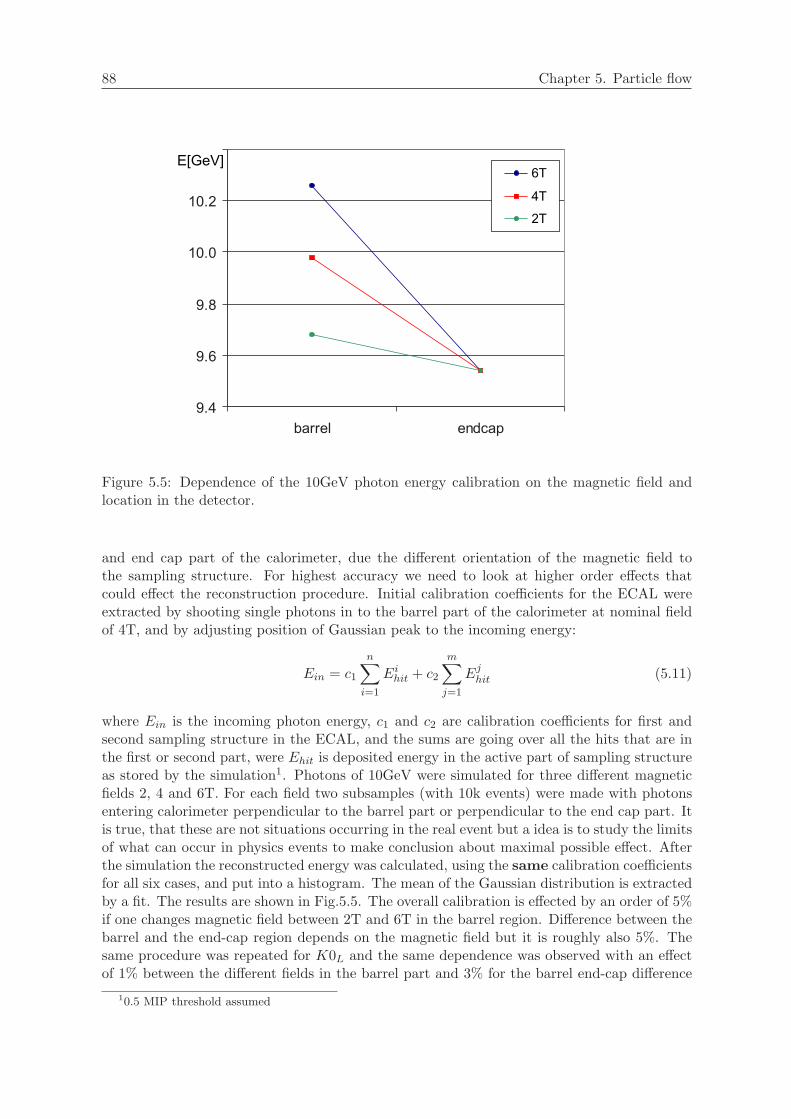
88 Chapter 5. Particle flow
Figure 5.5: Dependence of the 10GeV photon energy calibration on the magnetic field andlocation in the detector.
and end cap part of the calorimeter, due the different orientation of the magnetic field tothe sampling structure. For highest accuracy we need to look at higher order effects thatcould effect the reconstruction procedure. Initial calibration coefficients for the ECAL wereextracted by shooting single photons in to the barrel part of the calorimeter at nominal fieldof 4T, and by adjusting position of Gaussian peak to the incoming energy:
Ein = c1
n∑
i=1
Eihit + c2
m∑
j=1
Ejhit (5.11)
where Ein is the incoming photon energy, c1 and c2 are calibration coefficients for first andsecond sampling structure in the ECAL, and the sums are going over all the hits that are inthe first or second part, were Ehit is deposited energy in the active part of sampling structureas stored by the simulation1. Photons of 10GeV were simulated for three different magneticfields 2, 4 and 6T. For each field two subsamples (with 10k events) were made with photonsentering calorimeter perpendicular to the barrel part or perpendicular to the end cap part. Itis true, that these are not situations occurring in the real event but a idea is to study the limitsof what can occur in physics events to make conclusion about maximal possible effect. Afterthe simulation the reconstructed energy was calculated, using the same calibration coefficientsfor all six cases, and put into a histogram. The mean of the Gaussian distribution is extractedby a fit. The results are shown in Fig.5.5. The overall calibration is effected by an order of 5%if one changes magnetic field between 2T and 6T in the barrel region. Difference between thebarrel and the end-cap region depends on the magnetic field but it is roughly also 5%. Thesame procedure was repeated for K0L and the same dependence was observed with an effectof 1% between the different fields in the barrel part and 3% for the barrel end-cap difference
10.5 MIP threshold assumed
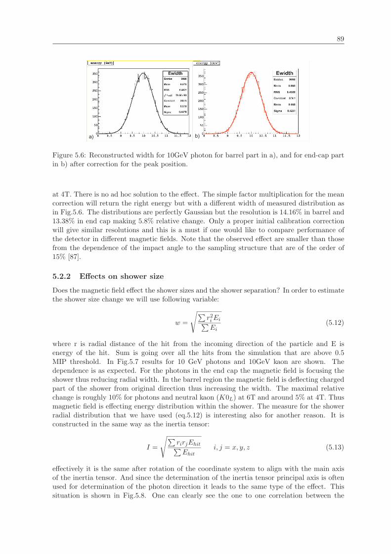
89
Figure 5.6: Reconstructed width for 10GeV photon for barrel part in a), and for end-cap partin b) after correction for the peak position.
at 4T. There is no ad hoc solution to the effect. The simple factor multiplication for the meancorrection will return the right energy but with a different width of measured distribution asin Fig.5.6. The distributions are perfectly Gaussian but the resolution is 14.16% in barrel and13.38% in end cap making 5.8% relative change. Only a proper initial calibration correctionwill give similar resolutions and this is a must if one would like to compare performance ofthe detector in different magnetic fields. Note that the observed effect are smaller than thosefrom the dependence of the impact angle to the sampling structure that are of the order of15% [87].
5.2.2 Effects on shower size
Does the magnetic field effect the shower sizes and the shower separation? In order to estimatethe shower size change we will use following variable:
w =
√∑r2iEi∑Ei
(5.12)
where r is radial distance of the hit from the incoming direction of the particle and E isenergy of the hit. Sum is going over all the hits from the simulation that are above 0.5MIP threshold. In Fig.5.7 results for 10 GeV photons and 10GeV kaon are shown. Thedependence is as expected. For the photons in the end cap the magnetic field is focusing theshower thus reducing radial width. In the barrel region the magnetic field is deflecting chargedpart of the shower from original direction thus increasing the width. The maximal relativechange is roughly 10% for photons and neutral kaon (K0L) at 6T and around 5% at 4T. Thusmagnetic field is effecting energy distribution within the shower. The measure for the showerradial distribution that we have used (eq.5.12) is interesting also for another reason. It isconstructed in the same way as the inertia tensor:
I =
√∑rirjEhit∑Ehit
i, j = x, y, z (5.13)
effectively it is the same after rotation of the coordinate system to align with the main axisof the inertia tensor. And since the determination of the inertia tensor principal axis is oftenused for determination of the photon direction it leads to the same type of the effect. Thissituation is shown in Fig.5.8. One can clearly see the one to one correlation between the

90 Chapter 5. Particle flow
Figure 5.7: Dependence of the radial shower size on the magnetic field and part of calorimeterfor 10GeV photons left (a), and 10GeV K0L right (b).
Figure 5.8: Dependence of direction determination on magnetic field for different parts ofcalorimeter for 10GeV photon sample.
91
Fig.5.7a and Fig.5.8. If one uses such a method for the determination of the photon direction,that is not optimal, error on the direction determination will start to depend significantly onthe magnetic field and part of the detector. Note that for 10GeV photons that we have used,the obtained resolution is significantly larger than the expected one (29.5mrad) for this energy[88]. One increases significantly the directional error of the reconstructed particle and violatesthe assumptions in the jet energy resolution estimation, that directional error is significantlysmaller than the energy measurement one, leading to a worser overall performance. This is aclear indicaiton theat drowing conclusions at this point should be done very carefully so as notto to attribute particular problem of the method used to test P-Flow with P-Flow in general.
5.2.3 Effects on full reconstruction
So far we have explained the field dependence on the level of single particles with effectson the percent level in terms of non-uniformity of the response over the detector (as fromsimulation) and changes in the shower sizes. Of significant interest is the detector performancein dependence on the magnetic field, since if strong, this will significantly limit room foroptimization of the detector. The vertex detector and tracking resolution goal give lowerlimit, first due to the amount of background, second due to the achievable point resolutionand number of measurement points on a fixed radius. Higher limit, except from the physicallimits, is from cost, mechanical constraints and already introduced low energy track efficiency.In order to check the performance of the reconstruction on the magnetic field (that is notpossible with pure calculation on the generator level), the same sample of Zpole hadronicevents was passed through the full detector simulation with different magnetic fields (2,4 and6T). After that the reconstruction was done using true information as stored by the simulation.Clusters are reconstructed by collecting the hits that belong to the particle according to theirID. In the case of several contributions to the same hit, assignment is made to the clusterof a particle with the highest contribution. Tracks were reconstructed from hits within thetracking system in same way. The only cut imposed was that the track should have at least3 hits. After that, clusters from the charged particles were discarded if the track exist, andthe true momentum was used. For neutral particles the measured energy is used and appliedto the true direction. After that a search for the secondary vertices was performed throughthe Monte Carlo particle tree and the particles were recombined with correct mass assignment(assuming correct identification of the decaying particle). The procedure is repeated until allreconstructed objects have reached interaction point. The mass of the event is then calculatedand put into a histogram. A double Gaussian fit was performed on the distributions (the firstone to account for central part of the distribution, and two half-Gaussians with center fixed onto the same mean to cover for the assymetric wings). The obtained mass distributions are inthe Fig.5.9. If we take the width of the central Gaussian as the measure for the reconstructedwidth and also fraction of the integral that is under this distribution as an efficiency estimator,one can come to a conclusion about field dependence. There is no B field dependence ofthe reconstruction if you comply with the assumptions introduced in eq.5.3, thusthis factorization is not appropriate to take into account B field effects of P-Flow.
The obtained width values (in Table 5.6) are within statistical errors (2%) and in goodagreement with the expected value of 1.51GeV for a given detector (according to eq.5.3).Small drop of the efficiency at 6T is due to the effective momentum cut by our 3 hits for trackcondition. A objection can be made that this will not hold for the real life reconstruction. Itis true but the intention was to show that there is no direct contribution term of magneticfield to the Particle Flow performance. Effects can, and should, be taken into account butthis can be done through the non P-Flow contributions, introduction of averaged or effective

92 Chapter 5. Particle flow
Figure 5.9: Reconstructed mass distributions for Zpole events in different magnetic fields.
Table 5.6: Dependence of perfect reconstruction on magnetic field in case of Zpole hadronicevents.
B field [T] σ[GeV ] fraction2 1.59 0.744 1.58 0.736 1.61 0.67

93
Figure 5.10: Contribution to the reconstructed width of hadronic Zpole events.
resolutions if no correction is applied, and adjusting the tracking efficiencies and acceptancecuts.
5.3 Conclusion
We have shown that the initial factorization of the contributions to the reconstruction perfor-mance 5.3 holds under the assumptions that is made on (5.1.2). It is thus useful to describeonly perfect Particle Flow (PPF), but not applicable to the more realistic setups. For thatreason factorization eq.5.5 is introduced that allows clear separation of all possible effects.Up to the level of accuracy used it was shown that ∼ 30%/
√E goal should be reachable for
all processes. An important issue of P-Flow performance is the dependence on the magneticfiled, since it is directly related to the cost. We have investigated the direct field effects (oncalibration and shower size), that are limited to ≤ 5% variation over the detector, and con-firmed that the expression eq.5.3 holds for different fields. This leads to the conclusion thatPPF is magnetic field independent. Effects from the possible breakdown of shower separationassumption and effects on the tracking efficiency acceptance can be incorporated as separatecontribution in the framework established by eq.5.5. This is indeed the largest achievementof our investigation of P-Flow, that a framework is established without any misleading andconfusing places. Fig.5.10 demonstrates that there are more ingredients to the picture thaninitially assumed, and treated so far opening room for further investigations.


Chapter 6
Particle Reconstruction in ILCDetector
6.1 Approach to Reconstruction
6.1.1 Reconstruction framework
It is not possible to talk about reconstruction of single type particles in a detector withouthaving full interconnection with rest of reconstruction procedure i.e. each particle specificmethod must be able to communicate with others and interchange acquired information inorder to get a consistent final particle identification and best possible performance. The photonfinding and reconstruction procedure that will be explained later was intended to work withina framework that has few distinct steps 1:
• trackingThis part is common to all reconstruction procedures and it is not specific. The mainprerequisite is to provide set of tracks with best momentum estimator at the end of thetrack closer to the calorimeter. Due to the lack of such information from the trackingcode available Monte Carlo truth from the simulation can be used as a supplement, butthe procedure does not rely on the type of the tracker used. Accurate extrapolation fromthe last track point till the face of the calorimeter is performed, a seed is created, thetrack is assigned to it and an extrapolation (with energy loss) through the calorimeteris made under assumption of energy loss for minimum ionizing particle.
• object creation and pre-clusteringAlthough at the end of simulation, or in the real detector, one has hits in a givenformat, LCIO [89] in our case, it might be preferable to change the structure containingthe information or to do additional calculation and store the output before the start offull reconstruction. There are several advantages for this approach: speed, quantitiesthat are frequently used and are not changing during execution can be calculated atearly stage only once and then stored; convenience, there is a well defined place whereall used attributes of any reconstruction object ( hit, cluster, seed etc.) are stored thusincreasing the readability of the code (within the framework used); maximization ofinput information for reconstruction procedure, by doing the initial preprocessing ofthe objects coming into reconstruction we try to maximize input information that is
1These steps should not be regarded as a part of sequential procedure, at some stage of reconstructionrepetition of some of them, or methods within, might be needed
95

96 Chapter 6. Particle Reconstruction in ILC Detector
available for decision making within algorithms and to follow the basic spiraling logic ofhighly performant reconstruction that is graduate(iterative) information collection thatleads to final result.
• reconstruction in the calorimeterThe major procedure for extraction of information from the calorimeter output.Thispart in the case of particles producing electromagnetic shower will be explained in detailin following sections.
• estimaton of physical quantities at interaciton point (IP)The event and it physical content were created at IP and the result of full reconstruc-tion should be set of best estimators of particle momenta and energies at the IP. Thispart of the procedure includes finding of secondary and tertiary vertices, photon conver-sions and kinks. Not applying this step will lead to inevitable performance drop of anyreconstruction procedure.
To the contrary of some ideas that the realization of this task is possible with separate-sequential procedure, 30%/
√E is an ambitional goal and only a well integrated and deep
event analysis can reach such performance. The accumulation of knowledge during the recon-struction procedure makes cross-jumps between any formal step in the procedure mandatoryin order to minimize the introduction of errors.
6.1.2 Requirements for the electromagnetic shower reconstruction
We want to reconstruct electromagnetic (EM) showers in ECAL originating both from photonsand from electrons or positrons. By reconstruction we assume a procedure that is both precise(returns the exact number of particles) and accurate (reproduces the intrinsic calorimeterresolution without introduction of any additional spread). Reconstruction in the ECAL is anessential part of the overall reconstruction. As shown in the previous chapter contributionof the ECAL resolution to the particle flow performance is at the ∼ 5% level assuming fullshower separation. The fraction of event energy for dominant processes (like e+e− →W+W−, tt) that is deposited in the ECAL is over 50% stressing the need to accomplish thefull shower separation both on the hardware and software level to acheave minimal impact ofECAL on the final PFA performance.
There is a huge spread of EM shower energies in physics events at a given center of massenergy. There are at least three distinct sources with different energy distributions. Those aredirect photons from the IP, photons from π0 decay, electrons and associated bremsstrahlungphotons. Direct photons from the IP have exponential distribution from zero with sharplydropping probability to higher energies. π0 distribution is peaked, with the position of the peakmoving logarithmically with growing center of mass energy. Electrons(positrons) rarely comefrom the hadron decays and are mostly coming directly from weak boson decays Z → e+e−
or W± → e±ν. Bremsstrahlung adds additional photons to the distribution and smears theinitial energy distribution of electrons. Additional effect is that amount of material betweenthe IP and the calorimeter, although small, makes photon conversion possible, introducinganother specific class for reconstruction 2, and additional source of electrons (positrons).
The energy distributions of electrons and photons were extracted from Zpole events passedthrough the full G4 detector simulation. Using the Monte Carlo information one can selectvarious subclasses of particles entering the calorimeter. On Fig. 6.1 is the energy distributionof electrons that covers full range between zero and half of the center of mass energy. Fig. 6.2
2in fact several depending on the point of conversion

97
Figure 6.1: Energy distribution of electrons(positrons) entering the calorimeter for events atZpole. In black total distribution, in blue conversion electrons, in red other decays electrons.
Figure 6.2: Energy distribution of photons entering the calorimeter for events at Zpole. Inblack total distribution, in blue photons from π0 decays, in red bremsstrahlung photons andin green other decay photons.
showes the distribution of photon energies with their subcomponents. Although the energy ofthe electromagnetic showers covers such huge range we would still prefer the reconstructionalgorithm with the same “dynamic range” to be capable of uniform treatment irrespectiveof the incoming energy. Even thoe we have such energy spread one should not forget thatthe mean energy of the particles in the fully hadronic events, to which the reconstructionperformance goal of 30%/
√E refers, rises logarithmically with center of mass energy and even
at 1TeV does not exceed 10GeV. Thus in the bulk of the cases algorithm will deal with showerswith small and intermediate energies.

98 Chapter 6. Particle Reconstruction in ILC Detector
6.2 Electromagnetic Shower
From the discovery of electromagnetic showers in 1933 [90, 91], they are one of the moststudied and best described phenomena in nature. Early on, significant and successful effortwas made in the development of the theory [92, 93, 94, 95] due to the fact that all dominantprocesses are exclusively governed by quantum electrodynamics3. Together with the largenumber of experiments accumulated knowledge led to the development of simulation toolslike EGS [101, 102, 103] that have been standard for almost 30 years (for latest comparisonwith data see [104]). Since we are talking about a well know facts in our introduction wewill mention only the most important features with a minimal amount of detail, these can befound in the abundant literature.
The most important processes involved in the generation of electromagnetic (EM) showersare: ionization losses, Cherenkov radiation, bremsstrahlung, photoelectric effect, Comptoneffect and pair production (for details see [96, 97]). From mentioned processes, bremsstrahlungand pair production are dominant for high-energy electrons and photons, respectively. Theircross sections become almost energy-independent for incoming energies À mec2
αZ1/3 , where α isthe fine-structure constant, Z is the atomic number of the medium andme is the electron mass.As a consequence, the radiation length, emerges as a natural unit of length and represents themean-path length of an electron in material and is given by:
1X0
= 4αNA
AZ(Z + ζ)r2e ln
183Z1/3
[cm2g−1] (6.1)
where NA is the Avogadro constant, A is atomic weight of the medium and re is the classicalelectron radius. ζ is a correction that takes into account the contribution of atomic electronsto the overall bremsstrahlung process with values between 1.2 and 1.4 [98]. Radiation lengthshave been calculated and tabulated [99]. Since we have same “natural”unit of length for elec-trons and photons the induced shower, shower development at same X0 thickness in differentmaterial should behave the same but this scaling is not perfect and photon and electron in-duced showers have to an extent different behavior [100]. We are interested in average behaviorof EM showers and the usage of those properties in the reconstruction, thus the introductionof second order corrections is possible and straight forward but not necessary for our purposeat the moment. When more than one absorber is present in the showering medium, the overallradiation length can be expressed as:
1X0
=∑
i
fiX0 i
(6.2)
where fi andX0 i are fraction by weight and the radiation length of the absorber i, respectively.Corresponding the density can be calculated from:
1ρ
=∑
i
fiρi
(6.3)
where ρi is the density of the i-th absorber. One of the basic answers from the theory (exper-iment) is how EM shower look like in terms of longitudinal and transversal profile, so we willinvestigate this properties in some detail.
3except for example (γ,n) reaction that is totally irrelevant for basic properties of the cascade
99
6.2.1 Longitudinal development
Due to the complexity of the processes involved descriptions of the EM shower were developedwith some approximations. One such model has been proposed by Rossi [105] and called“approximation B”. It takes into account radiation phenomena and pair production, togetherwith constant collision losses per unit of length. Since one is taking into account only someprocesses we need a unit that is expressing in which energy range they are really dominant.Such unit is critical energy usually defined as and energy at which electron loses as muchenergy in collision as in radiation [106] or as energy at which the ionization loss per radiationlength is equal to the electron energy [105]. One of the several approximate expressions is:
Ec = 2.66(X0
Z
A
)1.1[MeV ] (6.4)
The multiplication of electrons and positrons occur when their energy is much larger than thecritical energy and they get absorbed when collision losses become dominant. The number ofparticles increases rapidly with depth until the maximum, located at depth tmax, is reachedi.e. the longitudinal development of the shower has a maximum. The shower behavior canbe understood in a simplified way, following crude a approximation. Let E be the energy ofincoming photon, which after a depth of ≈ 1X0 generates e+e− pair of equal energy. After aadditional distance ≈ 1X0 both the electron and positron will emit a bremsstrahlung photon.By continuing the process, and assuming equal sharing among the generated particles, thenumber of them will double every radiation length. The number of particles at depth t isN(t) ≈ 2t, while their energy is Ep(t) ≈ E/N(t) = E2−t. When the particle energy isEp ≈ Ec multiplication will stop. This occurs at depth tmax for which Ec ≈ E2−tmax thus weexpect that tmax ≈ ln(E/Ec) Under approximation B, this maximum depends on the incomingenergy as ln(E/Ec). We can here introduce a natural variable for the expression of energy:
y =E
Ec(6.5)
and express the position of the maximum as:
tmax = T = a(ln(y) + c) [X0] (6.6)
where a=1.01, ce=-1.0 for electrons and cγ=-0.5 for photons as calculated by Rossi (newer moreaccurate calculation give a=1.0, ce=-0.5,cγ=0.5). Another useful parameter is the location ofthe center of gravity of the shower tcg that is given by
tcg = 1.01(ln(y) + d) [X0] (6.7)
where d=0.4 or 1.2 for electrons or photons, respectively. Longitudinal shower distribution isapproximately described by [107]:
dE
dt=
(βt)α−1β exp(−βt)Γ(α)
(6.8)
where β ≈ 0.5. The position of the cascade maximum is then:
tmax = T =α− 1β
= ln(y) + f [X0] (6.9)
were f = −0.5 for electrons and 0.5 for photons. The condition for 98% longitudinal contain-ment can be approximately given by
L(98%) ≈ 3tcg [X0] (6.10)
where tcg is given by eq.6.7.

100 Chapter 6. Particle Reconstruction in ILC Detector
6.2.2 Transverse development
Processes neglected in the longitudinal development are responsible for the transverse develop-ment of EM showers. During the cascade development the energy is degraded into low-energyelectrons via ionization, Compton scattering and photoelectric interactions, which generatedelectrons that dissipate their energy mainly by collision. Photoelectric and Compton scat-tering generate secondary electrons which are no longer aligned with the incoming photondirection and can even be emitted in the backward hemisphere in the case of photoelectricelectrons. Secondary Compton photons are no longer along the primary photon direction thuscontributing to the broadening of the cascade. Coulomb scattering of electrons that are notradiating any more also leads to the spread of electron directions away from the axes definedby the primary particle direction. The transverse depth unit of a cascade is the Moliere radiusdefined as [108, 109]:
RM =(ESEc
)X0 (6.11)
where ES =√
4πα mec
2 = 21.2MeV . In a material made out of several absorbers, an estimateof the overall Moliere radius can be obtained from:
1RM
=1ES
∑
i
fiEc,iX0,i
(6.12)
The 95% lateral containment for electromagnetic cascades is given by:
R(95%) = 2RM (6.13)
The transversal distribution of the shower depends on the calorimeter depth at which it ismeasured. At least a two-component structure is needed to describe the transverse profilewhich displays a narrow central (core) and broad peripheral part. The central part scales asRM and is mainly due to multiple scattering of fast electrons responsible for the depositionof most of the incident energy. The peripheral part is mainly due to the propagation ofphotons. Several two component parameterizations of the transverse shape as a function ofthe calorimeter depth exist and most of them have a double exponential form.
One of them is provided by the data obtained from a silicon calorimeter [112]. The lateralcascade distributions have been measured using a silicon calorimeter with tungsten and ura-nium as absorber for incoming electron energies of 2,4,6 GeV. Experimental data have beenfitted to radial energy distributions using the radial probability density function
F (r) =1N
exp[−√r
λ1] + C12 exp[− r
λ2 ]r
(6.14)
where λ21 and λ2 are in units of RM , C12 is the relative weight of the two components, r is the
radial distance in units of RM and N is coming from usual normalization condition:∫ 2π
0dφ
∫ ∞
0F (r)rdr = 1 (6.15)
We will use the following form:
f(r) = pfC(r) + (1− p)fT (r) = p2rR2
C
(r2 +R2C)2
+ (1− p)2rR2
T
(r2 +R2T )2
(6.16)
with 0 ≤ p ≤ 1, RC(RT ) are medians of the core (tail) component of radial profile and p isthe probability giving relative weight of the core component as proposed by Grindhammer

101
Table 6.1: Materials and their characteristics as implemented in G4 simulation for first struc-ture in ECAL
material d [mm] ρ[ gcm3 ] X0 [mm] Z A Ec[MeV ]
W 1.4 19.3 3.504 74 183.8 8.004G10 1.2 1.7 162.02 11 21.32 47.273Si 0.5 2.33 93.676 14 28.09 36.737
fiber 0.8 1.29 10−6 28516 7.3 14.61 0.0026effective 3.9 7.75 9.458 67.408 166.868 9.0804
[113]. The spatial energy distribution of the electromagnetic shower is then given by threeprobability density functions:
dE(~r) = Ef(t)dtf(r)drf(φ)dφ (6.17)
describing the longitudinal f(t) (eq.6.8), radial f(r) and azimuthal f(φ) energy distributions,where t stands for the longitudinal shower depth in units of radiational length, r is the radialdistance from the shower axis in units of Molier radius and φ is the azimuthal angle. Forconsideration of the average profile it is enough to assume a uniform distribution in φ i.e.f(φ) = 1/2π. The choice of the parameterization was driven more by practical than accuracyconsiderations. The requirement was that the code is still used and supported, possibly evenfurther developed. Parameterization as in [113] was used in past experiments (H1,Zeus), itwas implemented in the Geant3 framework, and is implemented in the Geant4 framework [114]and used for accelerated full simulation in CMS thus fully satisfying the requirements. Sincewe will not use it for simulation but for reconstruction, accuracy requirements are a bit morerelaxed and it can easily be exchanged with another if it is not suitable for our application.There is a low energy cutoff at which the parameterization can be used for simulation that isaround 800MeV [114]. This is not a problem for the usage in reconstruction as we will see forthe low energy region one needs a dedicated and different procedure anyhow.
Calorimeter parameters
In order to use the mentioned parameterization a detailed knowledge of the materials andtheir properties is needed. Tables 6.1,6.2,6.3 show lists of materials and their properties asimplemented in the detector simulation. Data from the tables were used according to formulaegiven in appendix C to calculate all needed variables for the computation of the spatial energydistribution eq.6.17 at a given point. Note that data in the tables correspond to the calorimeterin the original TESLA design 4. Calculation according to the formulae gives the Molier radiusfor the first ECAL structure as 22.08mm, for the second 13.84mm and 22.98mm for the HCAL.This makes the transversal segmentation around ∼ 0.5RM in ECAL and ∼ 0.8RM in HCALfor the cell size of 10mm in ECAL and 30mm in HCAL leaving enough measurement pointson the transferse profile if we take into account eq.6.13.
Table. 6.3 is here to remind us that the hadronic part of the calorimeter has a rathergood EM resolution (20%/
√E) and that methods in the algorithm are also applicable for
the location and extraction of the electromagnetic fraction in the hadronic cascade either forreconstruction or for software compensation. For data presented here, no attempt was madeto collect possible tails of the electromagnetic shower in the HCAL.
4corresponds to LDC00 model in full simulation

102 Chapter 6. Particle Reconstruction in ILC Detector
Table 6.2: Materials and their characteristics as implemented in G4 simulation for secondstructure in ECAL
material d [mm] ρ[ gcm3 ] X0 [mm] Z A Ec[MeV ]
W 4.2 19.3 3.504 74 183.8 8.004G10 1.2 1.7 162.02 11 21.32 47.273Si 0.5 2.33 93.676 14 28.09 36.737
fiber 0.8 1.29 10−6 28516 7.3 14.61 0.0026effective 6.7 12.5769 5.53 71.635 177.614 8.4709
Table 6.3: Materials and their characteristics as implemented in G4 simulation for the HCALmaterial d [mm] ρ[ g
cm3 ] X0 [mm] Z A Ec[MeV ]Fe 20.0 19.3 17.59 26 55.85 20.653
scintillator 5.0 1.7 162.02 11 21.32 47.273fiber 1.5 1.29 10−6 28516 7.3 14.61 0.0026
effective 26.5 6.134 23.06 25.318 54.354 21.285
6.3 Photon finding algorithm
Since we often hear about an “imaging” calorimeters the basic idea of the algorithm is touse the picture processing methods to extract the needed information. Lets use our EMshower average energy density profile and integrate it over the ECAL layers and rings withinlayers around the initial photon direction with a width equal to the cell size. This defines thefunction:
f(r, n, d) =∫ r+d/2
r−d/2
∫ n+1
n
∫ 2π
0dE(~r)drdtdφ (6.18)
where r is radius, n layer number and d cell size. If we plot this funciton with some numberof thresholds as in Fig.6.3 we can have estimate of the distribution of energy deposited incells. We can see that on the basis of this picture in the ideal case we would be able todistinguish how many photons we have (by the number of red zones), and to separate closeby photons in some color (second blue shade). The “picture” taken with the calorimeterwill be smeared due to the physics (fluctuations in the shower) and due to the finite cellsize since the radius is not changing in infinitesimal but finite steps (egqual to the cell size).In a highly granular calorimeter as the one proposed for the ILC detector this smearing issmall and enough information survives that our idea can be applied. This is the essence ofthe algorithm. From some initial set of data containing only a monochromatic set of pointsin space we are painting them according to the deposited energy with some pallet and thentrying to distingush features as one would do by naked eye. As a counter measure to thesmearing additional noise reduction procedure is intorduced in order to remove ”bad”pixels.This establishes an integrated procedure for both localization of single and separation of closeby showers.
6.3.1 Algorithm steps
The algorithm tries to merge two distinct approaches to the reconstruction, one with the pre-dominant use of energy information and second with predominant use of topology information.My personal opinion is that only an optimal balance of this who sides can give you the wanted

103
Figure 6.3: Photon profile 10GeV and 4 GeV photon, energy density distribution integratedover layers and rings of cell size width.
Figure 6.4: General layout of the photon finder algorithm.
performance. Fig. 6.4 shows the basic layout of the algorithm. Now we will go through eachstep of the algorithm in some detail.

104 Chapter 6. Particle Reconstruction in ILC Detector
Figure 6.5: Dimensions of the ECAL cell volume, thickness (h) depends on the amount ofabsorber.
Figure 6.6: Transformation of the cell coordinates to isotropic space a) real cell arrangementb) cell coordinates after transformation, where d is cell size.
ECAL hits
The ECAL volume is divided by segmentation (both longitudinal and transversal) into quantafor which we have separate information from the detector - ECAL cells. ECAL cell, as shownin Fig.6.5 for 1×1cm transversal segmentation, has a thickness that varies from 3.9-6.9mm indifferent zones (first or second sampling structure) or in different designs of the ECAL. Notethat this is not a cubic volume. Each of these volumes has a unique ID, measured energy(assumed to be in GeV) and coordinate (characteristic point within the cell volume - in thesimulation geometrical center of active material). This information stored together, we willcall hit. Assuming that proper calibration is performed and that the mentioned informationis stored in LCIO hit classes, the treatment of simulated and real data will not differ. At theinitial stage calibrated hits together with the information about minimum ionizing particle(MIP) signal size are passed to the algorithm. Information is copied to the internal hit classand amplitudes in units of MIP are calculated and stored.
Pre-calculation
From the knowledge about the shower development one expects rather compact object withoutdiscontinuities arising in the calorimeter, thus the natural choice for collecting hits is a nearestneighbor (NN) type of clustering. For NN clustering one needs to define a metric in whichthe distance5 between objects is calculated and the cutoff value for the distance at which weconsider two objects to be neighbors. Due to the fact that the cell volume is not a cubic one,a simple Euclidian metric and one cutoff on the physical distance between hits will not work.There are two possible solutions to this problem. One can define a rather complex metricand work in the cell ID space or we can transform the cell coordinates into an isotropic spaceand use a simple distance measure. Both approaches should give the same result but due totechnical reasons transformation was chosen as the preferred solution. The basic requirement
5not necessary physical length
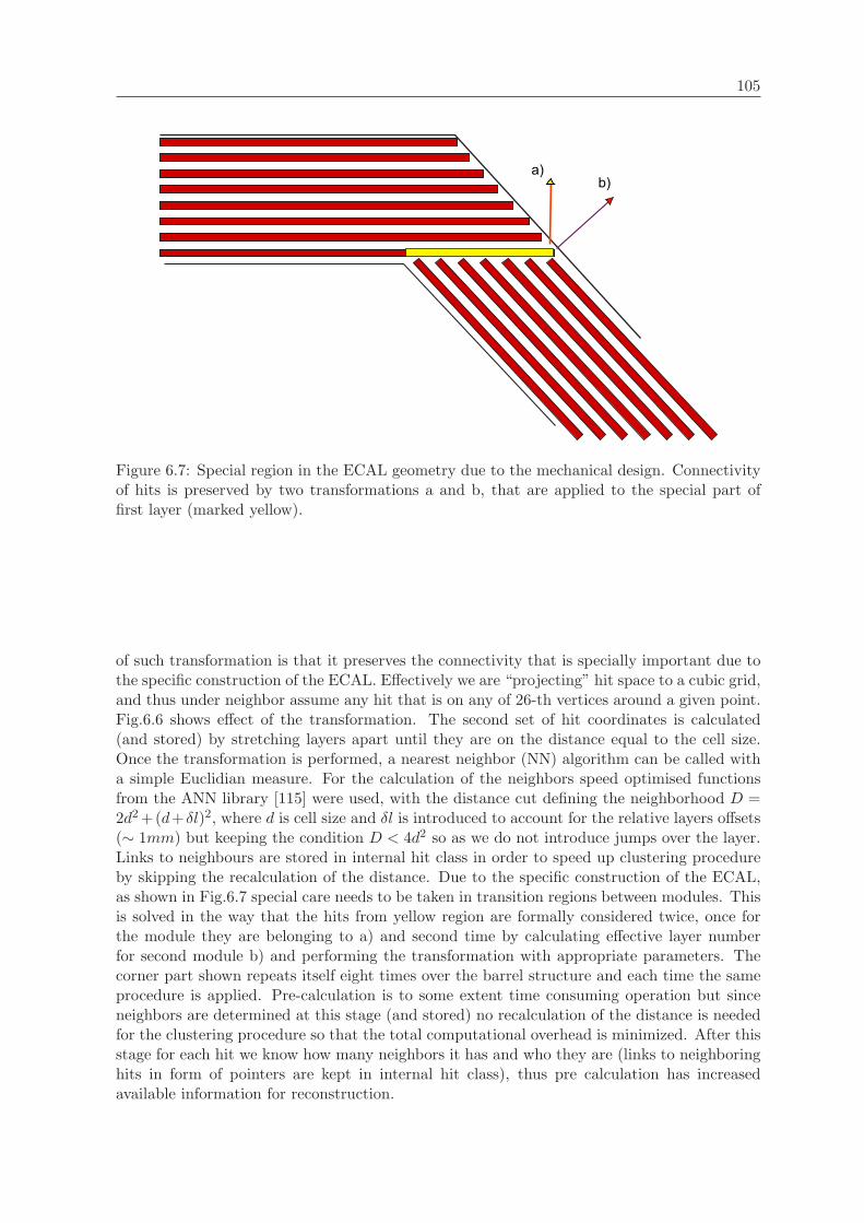
105
Figure 6.7: Special region in the ECAL geometry due to the mechanical design. Connectivityof hits is preserved by two transformations a and b, that are applied to the special part offirst layer (marked yellow).
of such transformation is that it preserves the connectivity that is specially important due tothe specific construction of the ECAL. Effectively we are “projecting” hit space to a cubic grid,and thus under neighbor assume any hit that is on any of 26-th vertices around a given point.Fig.6.6 shows effect of the transformation. The second set of hit coordinates is calculated(and stored) by stretching layers apart until they are on the distance equal to the cell size.Once the transformation is performed, a nearest neighbor (NN) algorithm can be called witha simple Euclidian measure. For the calculation of the neighbors speed optimised functionsfrom the ANN library [115] were used, with the distance cut defining the neighborhood D =2d2 +(d+δl)2, where d is cell size and δl is introduced to account for the relative layers offsets(∼ 1mm) but keeping the condition D < 4d2 so as we do not introduce jumps over the layer.Links to neighbours are stored in internal hit class in order to speed up clustering procedureby skipping the recalculation of the distance. Due to the specific construction of the ECAL,as shown in Fig.6.7 special care needs to be taken in transition regions between modules. Thisis solved in the way that the hits from yellow region are formally considered twice, once forthe module they are belonging to a) and second time by calculating effective layer numberfor second module b) and performing the transformation with appropriate parameters. Thecorner part shown repeats itself eight times over the barrel structure and each time the sameprocedure is applied. Pre-calculation is to some extent time consuming operation but sinceneighbors are determined at this stage (and stored) no recalculation of the distance is neededfor the clustering procedure so that the total computational overhead is minimized. After thisstage for each hit we know how many neighbors it has and who they are (links to neighboringhits in form of pointers are kept in internal hit class), thus pre calculation has increasedavailable information for reconstruction.
106 Chapter 6. Particle Reconstruction in ILC Detector
Topological cleaning
Now it is possible to benefit from the additional knowledge about the event by cleaningthe picture before the crucial step of core localization and identification. By topologicalcleaning we assume removing hits with less thenM neighbors from the intermediate processingin algorithm6. Topological cleaning is introduced from general considerations for algorithmworking on full physics events where one would like to clean the picture from the thingsthat are obviously not photons: isolated hits and track segments for which we don’t need toconsider energy information. Effects of the topological cleaning are shown on Fig.6.8. Onlysome hits on the surface of the electromagnetic shower are removed and at the same time themuon track is fully erased. This step is not mandatory, and algorithm can work without it.Photon finding in this algorithm is based on recognition of the dense part of the shower i.e.“core” so why would one like to do a separation of hits on the topology? There is a correlationbetween the energy information and the topological one but this is not the main reason forthis approach. Two major reasons for this step are: - due to the Landau distribution of the hitenergy on track segments in the calorimeter, hits can have almost arbitrary energy; - the sameis true for the neutron hits that are randomly spread around. With topological cleaning thesehits are removed from consideration in a natural way and can be passed to other algorithmswithin the reconstruction for processing. Second by topological cleaning we are smoothingthe surface of the shower and reducing the problems with natural fluctuations. The onlysignificant argument against the usage is the problem with low energy photons (≤ 0.5GeV ).Not only that such photons have ill defined shape that is hard to recognize with any kindof the procedure, but in a dense calorimeter they start to behave more and more track likei.e their energy density distribution is so contained in a volume comparable with the cell sizethat there are not enough hits satisfying selection criteria to construct the core. This leadsto a drop of the efficiency in this energy range and is not the responsibility of the topologicalcleaning alone but a result of the rather complex interplay with other algorithm stearingparameters (specially minimal number of hits in NN cluster). If one decides to use this stepin the algorithm only hits that pass the cut will be used in the following steps until the finalphoton construction when naturally all the hits7 are considered.
Central loop
In order to locate the core parts of electromagnetic showers we will do an energy scan over hits.All the hits still available (all of them if no topological cleaning) are split into N subsets withthe condition Ehit > Ti where Ti is i-th threshold (level) 0 ≤ i < N . It is obvious that thiskind of spiting is not exclusive thus some of the hits will appear in more than one category, andit is exactly what we want for the pattern recognition step. After such splitting NN clusteringis performed on each subset (hits are clustered only with the neighbors belonging to a givenset). By doing this after finishing N-loops we have M (where M ≤ N depending on highest γenergy in the event and chosen parameters of the algorithm) sets of clusters made at differentenergy levels and this set of clusters is the input information into pattern recognition. OnFig.6.9 all the thresholds used are plotted on top of the hit energy distribution in MIP unitsfor 5GeV photon. The first threshold should be same as the calibration one thus including allavailable hits.
Why do we need N levels, and could N be 1 or 2? In order to answer this question we shouldlook at hit energy distribution for showers from different ends of spectrum. In Fig.6.10 the
6central loop and pattern recognition7may not be true if it is used in synergy with other algorithms

107
Figure 6.8: Effect of topological cleaning. On the picture are photon and muon close by. Inred are hits left after such procedure in blue those removed, cut M ≤ 4.
Figure 6.9: Energy distribution for ECAL hits from 5GeV photon with all default thresholds(except first one).

108 Chapter 6. Particle Reconstruction in ILC Detector
Figure 6.10: Energy distribution for ECAL hits, in blue 1GeV photon in red 20GeV photon.Normalized to maximum.
Figure 6.11: Expected pattern after threshold clustering for isolated EM shower.
energy distribution of hits from 1GeV and 20GeV showers is plotted. If we keep in mind thatdistribution for energies between 1 and 20 GeV will lie between the two curves, and assumetwo close by photons, it is clear that the separation simply on the basis of the thresholdingand clustering would be possible with good efficiency, only for a pair of energies and particularextent of overlap. One or two thresholds is enough if one would use it for image cleaning (thatis done by topology in this algorithm) and the core finding by another procedure (peak findingon spherical projection, clustering in θ−φ or another approach). We are not only interested tofind in finding bulk electromagnetic showers but also to have good close by shower separation.Note that thresholds are more densely covering lower part of the hit energy spectrum (Fig.6.9)exactly for the reason to have good separation over the full energy range.
Pattern recognition
This is the step of the procedure where the decision about the number of photon candidatesis made and the photon candidates are produced. Initially all lowest level clusters are labeled

109
Figure 6.12: Expected patterns after threshold clustering in case of fluctuations a) and twoclose by photons b).
as photon candidates. What would be the distinctive sign of a single photon? As shown inFig.6.11 according to our threshold selection and neglecting the fluctuations one would havea repeating structure of clusters in which each level cluster will enclose only one cluster ofhigher level. If this is the case lowest level cluster is kept as a core of the electromagneticshower. The lowest level cluster is natural choice since it contains the maximal fraction of thefull shower energy and will give the most accurate estimate of the incoming energy in nextstep.
If at some level i+1 we have 2 or more clusters a decision needs to be made to considerthem as two “cores” of electromagnetic shower or one needs to be kept and other discarded.Natural fluctuations of the shower tend to create false cores. Due to the lateral containmentof the shower over the small number of cells and NN clustering procedure these ghosts areappearing mostly in the second part of the shower development as in Fig.6.12 a). At thesame time we can have two close by photons that are overlapping to some extent so that theirseparation is achieved only at i-th level Fig.6.12 b). In the case of two real photons the startingpoint need not to be at the same calorimeter depth and is exponentially distributed from theface of the calorimeter along the incoming direction. Thus there is an angle between thedirection connecting shower centers with respect to the incoming direction. This angle is not90 degrees (as it would be for same starting point, same incoming energy and no fluctuations)but is on the average significantly larger then the angle for the ghost cores. This gives us apowerful separation criteria. The second separation criteria is distance of two core candidates.For the fake cores NN cluster is most probably split due to the fluctuations in one layer ofthe calorimeter and in the case of two real photons we have much wider distribution. Thesedifferences in behavior are used in a cone cut as on Fig.6.13. A cone with some opening angle(parameter of the algorithm) is constructed from the center of one cluster along the assumeddirection of incoming particle. If the center of second cluster is within the cone and distanceis small enough this cluster is discarded as a fluctuation as in Fig.6.13 a). If the second clusteron level i is outside of the cone as in Fig.6.13 b) the initial core is discarded and two new onesare formed.
The performance of this part of the procedure is steered with several parameters for cluster-ing, splitting (initial “core” is deactivated and two new ones emerge), discarding and merging(two cores of the same level are merged and are considered as one further one). The merging

110 Chapter 6. Particle Reconstruction in ILC Detector
Figure 6.13: Cut based separation used to discriminate between fluctuations in case a) andtwo close by photons in case b). Triangle represents cut cone.
procedure is a additional correction procedure in order to minimize the software induced er-rors. Imagine a situation from Fig.6.13 in such a way that left core in the part b) is replacedby part a). Now we have 3 cores at given level, two correct ones and one fake. If two arechosen to be new cores the runaway fraction, third core, is then merged into one of otherseven thoe is not connected in nearest neighbor meaning. This merging procedure is not af-fecting the number of cores found but is needed for the next step that is energy estimation.If one would throw away fluctuation fragment we would significantly decrease the accuracyfor energy estimation procedure. The result of the pattern recognition step is a set of cores -photon candidates.
Energy estimation
After pattern recognition we have a set of core clusters i.e. photon candidates. For eachof these candidates we need a estimation of the incoming photon energy. Why we need thiswhen calorimeter measures the energy? We need such a step in order to collect the full photonenergy (in distant and isolated hits) and to have more accurate photon profile construction.Since the sizes of the photon profile vary logarithmically with energy there is no need fora extremely accurate but still want precise estimator. This step is in a sense calibrationprocedure. Large samples of photons are passed through the simulation and the algorithmwith the modification that energy of clusters at each level is stored. After that incomingenergy is parameterized as a function of core energy and threshold level. As one can see fromFig.6.14 linear parameterization of the form
Eγ = a+ bEcore (6.19)
is sufficient for given level. Once this lookup table for given detector is made it’s easy to makea function:
Eγ = f(Eicore, i, detector) (6.20)
that gives estimation of incoming photon energy, where i stands for threshold level and detectorimplies that this parameterization needs to be done for particular choice of detector (sampling,cell size, simulation parameters etc.), and algorithm parameters. Even tho procedure forcreation of incoming energy estimation function 6.20 is straight forward it can be lengthyprocedure if one would like to cover larger energy range or make several of them for detectoroptimization purpose.

111
Figure 6.14: Example of the energy estimation fit for 12 GeVphotons. On abscise energy of the cluster on level 4, on ordinateenergy of true cluster.
Photon construction
After energy estimation one has all the variables needed to construct a photon on the basis of3D model. The parameters are energy, direction (one can choose between IP-center of the coreor inertia tensor direction) and starting point. At this place topological information can behelpful since one can neglect isolated hits when searching for hit closest to the ECAL face alongthe chosen direction as an approximation of the starting point. Once all input parameters arecalculated it is possible to calculate the energy density for a photon at the position of eachhit. Why energy density and not the integral over the cell volume? Due to the complexityof the energy density function for the 3D profile and arbitrary orientation of the cell volumeto the direction of the photon one would need a complicated and time consuming numericalintegration procedure at this stage without a clear gain. At this stage estimator is neededthat will satisfy two conditions: It has the knowledge about the shape (in order no to pickup arbitrary distant hits) and it is proportional to the deposited energy in the cell volume (inorder to be used for separation in case of close by γ(e)). Value of energy density distributionat a hit position is such estimator, first requirement it satisfies automatically. We are makingreplacement of the kind:
∫
cellf(r1, t1, E1)dr1dt1 ⇒ f(r1, t1, E1) (6.21)
that should satisfy:∫
cellf(r1, t1, E1)dr1dt1 >
∫
cellf(r2, t2, E2)dr2dt2 ⇔ f(r1, t1, E1) > f(r2, t2, E2) (6.22)
It can be proven by hand or some mathematical computation package [118] that inequalityholds for radial functions of the form that we have in eq.6.16:
Ar
(r2 +B)2(6.23)

112 Chapter 6. Particle Reconstruction in ILC Detector
if r1 > r2. Full energy density distribution of eq.6.17 is used to calculate “probability” that hitbelongs to a given photon candidate. In order to provide user with the full information neededfor each spatial point requested value of the estimator and radial distance from the directionis returned. Now we can assign a estimator to each available hit. By available hits we meanall the hits in ECAL irrespective of their topology if they are not assigned by anotherprocedure. Good example for this is Fig. 6.8 it means that muon “track” hits in the ECALare already assigned to the muon and are not subjected to this part of the procedure. Infinal stage after processing hits with multiple contributions in some way either deterministic(assignment to one or another photon candidate - used in the algorithm at the moment) orweighted ( i.e. energy shearing between the photon candidates with some weight) one shouldhave full set of hits that can be stored in a cluster class of choice. At this step or any laterduring reconstruction procedure quality check is needed before final assignment- quality check is left to be performed by user.
6.3.2 Summary of steering parameters
Parameters of the detector as geometry and materials although used in algorithm are notvariables since whole calibration procedure for the energy estimation step would need to beredone (material change is changing the shower development and at the same time integrals ofphoton shower energy density distribution over the cell volume thus energy esitimation on thebase of the cluster with given treshold and topology characteristic will be affected and in orderto preserve reachable accuracy level of shuch procedure it needs ot be repeated). Sequence oftasks would be to adjust the parameters of the algorithm (if not satisfied with the default)using an old calibration and after that redo the calibration for the final data processing. Hereis full set of steering parameters for the algorithm as it used for the evaluation of performancethat will be presented later. The steering parameters of the algorithm are:
• Topological cleaning threshold - Minimal number of neighbors that hit needs to have inorder to be considered within photon candidate search routine.Default value M = 4.
• Number of threshold levels- number of subsets in which the hits will be divided forinternal clustering and pattern recognition. Choice of particular number of levels shouldbe made on expected energy range of photons (electrons), precision of search, amount ofwork needed for preparation of energy calibration procedure and speed penalty that isacceptable. Number of levels is arbitrary but due to the LCIO Cluster class properties(level of the photon candidate is stored in type bit-field by setting appropriate bit to 1)it’s limited on 16 for larger number you would need to do the coding on your own!Default value N = 10
• Threshold levels - particular choice of N cut levels once N is determined in previousstep (in units of MIP)Default value 0.1, 1.5, 2.5, 4.0, 6.0, 9.0, 16.0, 26.0, 41.0, 65.0
• Minimal cluster size, in number of hits, for 0-th level cluster - As already stated initiallyall 0-th level clusters are considered as photon candidates thus this parameter affects theinitially number of candidates and thus the efficiency of algorithm. Proper value needsto be chosen depending on actual value of topological cleaning parameter.Default value 4
• Minimal cluster size, in number of hits, for i-th levelDefault value 4

113
Figure 6.15: Transition region between ECAL barrel and end cap. EM shower distributionis represented with red zones on the left, algorithm for the fake suppression after preliminaryphoton construction on the right.
• Splitting condition - Cosine of the cone opening angle plus the distance between thesplitted clusters (in mm). Plus additional parameter to suppress fluctuation called Rcutthat is putting limit on the ratio of hits in next level to the number in previous.Default value 0.9 35mm 0.4
• Energy density threshold - formally energy density function of the 3D photon modelhas non zero value even outside of the detector since longitudinal and transversal profilefunctions are normalized on the 0 to infinity range. For practical purpose this is of corsenonsense. In order to limit range in which one would try to assign hits to a photon andstill collect full energy some cutoff value needs to be chosen. This cut naturally arisesfrom the fact that we have a 0.5MIP calibration threshold thus at some value of energydensity it’s integral over the cell volume will not reach 0.5MIP energy.Default value 0.00001GeV X0
−1RM−1
6.3.3 Algorithm performance
Single photon
For testing algorithm performance single photon events were generated over the larger energyrange, with uniform distribution in θ and φ, using MOKKA LDC00 02Sc model. In order tohave some reference performance values obtained from so far best reconstruction tool Pandora[116][117] were used for comparison. Definition of efficiencies for single photon case is: “Shootexactly one photon into detector and expect to reconstruct exactly one “. Thus with singlephoton case we can test proper reconstruction and confirm that usual problem of the generalclustering approach - splitting is solved. Due to the possibility of conversion in to the e+e− pairevents were selected on the base of true information available from MC simulation. Conditionis that endpoint of the photon is located in the ECAL. This condition reduces incoming sampleby 20% but assures that we have exactly one photon entering the calorimeter. This cut isapplied in all single photon samples.
Transition region of the two major parts of the ECAL (barrel and end cap) is makingserious challenge for reconstruction and identification of EM shower. Current implementationin the MOKKA has empty space that will probably be partially or fully filled with material(cables,TPC support). With no or with little material this transition region acts as a mag-netic spectrometer dividing neutral and charged part of the EM shower leading to considerable

114 Chapter 6. Particle Reconstruction in ILC Detector
spatial spread in the second part of the shower that is measured with end cap part as demon-strated in Fig.6.15. In order to isolate these effect one can define 200mm long region withinthe barrel,(measured from the edges of the barrel) that will be called corner region. On thebasis of the Monte Carlo information we can separte (or remove) photons that start to showerwithin this zone. Dedicated procedure needs to be developed to cover reconstruction in thissegment of the detector. Loss of the recognizable and characteristic shape of the EM showerwill also make neutral hadron shower separation significantly harder. Effects of the cornerregion on the reconstruction performance will naturally depend on the angular distributionof the process in question and performance of the software compensation for these effects.In order to determine the true algorithm performance and exclude detector non uniformityeffects for photons above 1GeV there was additional event selection cut that excludes thecorner region of the ECAL thus giving clean algorithm performance. In order to estimate sizeof the effect same samples were processed with and without this cut.
As already mentioned quality check is left to be performed by user so that algorithm canbe integrated within various frameworks. In order to estimate performance rudimentary cor-rection procedure was developed. This is still not identification procedure in its full meaning!Most of the tools used like neural networks [119] and H matrix [120], or others do not constructcluster but just give the probability i.e. photon ID for cluster created in another procedure.Here we are making conceptual jump from disconnected and sequential procedure to iterativeone:
• clustering → particle ID to the integrated and essentially recursive approach to
• clustering → validation → clustering → validation ... until all reconstructed object fitto the desired criteria.
Procedure developed is in fact a fraction of validation step that would contain also properphoton ID. Once the hits are preliminary assigned to the found cores one can check theconsistency of the calibration energy and the energy collected in hits. Fakes have low energyand after the assignment of hits less energy then there is to be expected. This feature wasused in the procedure sketched on Fig.6.15.
After preliminary assignment of hits to found cores energy of collected hits is calculated.Ratio of the collected energy and the estimated incoming energy from the calibration procedureis made.
Er =EcollectedEincoming
(6.24)
This quantity was used to make logical rejection criteria in the form:
if(not (Er < 0.5 or (Er < 0.6 and Eincoming < 0.6GeV ))
)(6.25)
If condition is satisfied no action is taken. If not preliminary photon candidate is deletedand it’s hits are reassigned to remaining photons. Loop is repeated until all the photons areprocessed and pass the criteria. This leads to reduction of number of reconstructed particlesfrom N to M. In order to demonstrate the effect of this step number of cores i.e. prelimi-nary photons was plotted on the Fig.6.16 and is stated separately in the full result tables inappendix.
In Fig.6.16 and Table 6.4 results for energy range 1-40GeV are presented for full detector.In order to see the impact of the post processing procedure there is additional column labeled“core” that is representing the performance on the level after pattern recognition (withoutfake suppression). We can see that general clustering approach as expected performs well atlow energies and then efficiency drops rather fast due to the splitting of showers into several

115
Figure 6.16: Single photon efficiency after core finding (in green), final result after fake sup-pression (in red) in comparison with Pandora-PFA (in blue).
Table 6.4: Single photon reconstruction efficiencies for single photon events, summary table.Full dataset.
Energy [GeV ] core [%] algorithm [%] Pandora-PFA[%]1.0 96.32 99.4 99.03.0 97.76 99.7 98.75.0 97.60 99.1 97.29.0 96.86 99.0 92.9
16.0 93.80 98.6 87.620.0 92.80 98.4 83.440.0 86.50 98.3 68.11

116 Chapter 6. Particle Reconstruction in ILC Detector
Figure 6.17: Single photon efficiency after core finding (in green), final result after fake suppres-sion (in red) in comparison with Pandora-PFA (in blue) with ECAL corner region excluded.
clusters. Situation at the core finding stage is intermediate one, there is some basic level offakes but the energy dependence is already much more flat and performance at higher energiesis significantly better then with general clustering. After fake suppression final performanceis now almost flat and at expected level.
In Fig.6.17 and Table 6.5 are results for the pure reconstruction performance since cornerregion event were removed from the data sample. Now one can clearly see the linear drop ofthe simple clustering and flat performance of explained algorithm.
Difference in performance depending on the inclusion of barrel end-cap transition regionis demonstrated in Fig.6.18. At lower energies (below 3GeV) effect is almost negligible. Thisis due to the fact that size of shower in this energy region is small, plus solid angle for theregion which needs to be hit in order to produce recognizable signature in both parts of ECALis infinitesimally small. When we go the the higher energies size of the shower grows, as wellas solid angle of the region in which leaking part of the shower from barrel is recognized aphoton in the end-cap. This region is represented in almost linear drop in efficiency from3-20GeV. For 20-40GeV region we have reached situation that none of the incoming photonswithin this zone is reconstructed as one so the total effect is proportional to the integral ofthe incoming photon angular distribution over the zone. Performance of both investigatedreconstruction approaches is same in this zone and can be shortly described by you shoot onein you get arbitrary number of reconstructed particles at output. This confirms the statementthat dedicated procedure need to be developed to deal with this region.
Additional check was made for the performance in the low energy region (bellow 1GeV). Inthis region raison for efficiency drop is now pure inefficiency that is to say there is 1 incoming

117
98
98.5
99
99.5
100
100.5
0 10 20 30 40 50
Egamma [GeV]
1g
am
ma
eff
[%]
with corner
without corner
Figure 6.18: Single photon efficiencies for the algorithm for full data set (in red), and withcorner region excluded (in blue).
Table 6.5: Single photon reconstruction efficiencies for single photon events, summary table.Without events going to the barrel end-cap transition region
Energy [GeV ] core [%] algorithm [%] Pandora-PFA[%]0.3 65.55 65.18 57.860.4 83.86 84.73 77.180.5 92.05 94.57 90.170.7 95.98 99.00 99.01
0.85 96.12 99.31 99.191.0 96.44 99.53 99.193.0 98.27 99.81 98.945.0 98.37 99.87 97.719.0 97.76 99.89 94.01
16.0 94.85 99.90 88.8020.0 94.27 99.83 84.8540.0 88.14 99.93 70.63

118 Chapter 6. Particle Reconstruction in ILC Detector
Figure 6.19: Single photon reconstruction efficiencies for low energy photons. Red line marksthe 95% efficiency crossing point at 0.5GeV.
photon but there are no reconstructed particles. From the Fig.6.19 and the table 6.5 it is clearthat improvement over the straight clustering approach is tiny and that 95% efficiency level iscrossed at 0.5GeV. Drop of the efficiency is sharp going to the lower energies and follows oneto one direct clustering of Pandora. There are several raison for such a behavior low energyphotons do not have a well defined shape as those on higher energies, relative fluctuationsin number of hits and their distribution is higher and the parameters of the algorithm wereunchanged in order to test possibility to cover full energy range with one set of parameters.Any kind of reconstruction will have a hard time making robust procedure to detect low energyphotons and distinguish them from the background coming from other showers in full physicsevent. At the present stage algorithm does not have satisfactory performance for the energiesbelow 0.5GeV.
Neutral pions
Neutral pion were also generated in order to test the performance of the algorithm. Withpions we can check at the same time proper counting as in single photon case but also properseparation of close by photons with different energies. Proper separation of showers willrepresent itself in the width of the reconstructed mass distribution and pion reconstrucitoncan improve overall PFA reconstruction [121]. Mass can be calculated in usual way:
mγγ =√
2Eγ1Eγ2(1− cos θγγ) (6.26)
π0 samples were generated in flat distributions in θ and φ over the detector. Events wereselected according the MC truth information so that both photons reach the ECAL withoutconversion. Additional cut was implemented, as in single photon case (If any of the photons
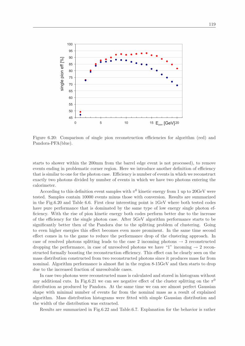
119
Figure 6.20: Comparison of single pion reconstruction efficiencies for algorithm (red) andPandora-PFA(blue).
starts to shower within the 200mm from the barrel edge event is not processed), to removeevents ending in problematic corner region. Here we introduce another definition of efficiencythat is similar to one for the photon case. Efficiency is number of events in which we reconstructexactly two photons divided by number of events in which we have two photons entering thecalorimeter.
According to this definition event samples with π0 kinetic energy from 1 up to 20GeV weretested. Samples contain 10000 events minus those with conversion. Results are summarizedin the Fig.6.20 and Table 6.6. First clear interesting point is 1GeV where both tested codeshave pure performance that is dominated by the same type of low energy single photon ef-ficiency. With the rise of pion kinetic energy both codes perform better due to the increaseof the efficiency for the single photon case. After 5GeV algorithm performance starts to besignificantly better then of the Pandora due to the splitting problem of clustering. Goingto even higher energies this effect becomes even more prominent. In the same time secondeffect comes in to the game to reduce the performance drop of the clustering approach. Incase of resolved photons splitting leads to the case 2 incoming photons → 3 reconstructeddropping the performance, in case of unresolved photons we have “1” incoming → 2 recon-structed formally boosting the reconstruction efficiency. This effect can be clearly seen on themass distribution constructed from two reconstructed photons since it produces mass far fromnominal. Algorithm performance is almost flat in the region 8-15GeV and then starts to dropdue to the increased fraction of unresolvable cases.
In case two photons were reconstructed mass is calculated and stored in histogram withoutany additional cuts. In Fig.6.21 we can see negative effect of the cluster splitting on the π0
distribution as produced by Pandora. At the same time we can see almost perfect Gaussianshape with minimal number of events far from the nominal mass as a result of explainedalgorithm. Mass distribution histograms were fitted with simple Gaussian distribution andthe width of the distribution was extracted.
Results are summarized in Fig.6.22 and Table.6.7. Explanation for the behavior is rather

120 Chapter 6. Particle Reconstruction in ILC Detector
Table 6.6: Pion reconstruction efficiencies for single pion events, summary table. Withoutevents going to the barrel end-cap transition region
π0 Energy [GeV ] algorithm [%] Pandora-PFA[%]1.0 49.24 47.142.0 73.15 72.863.0 80.36 79.194.0 85.06 83.825.0 87.83 86.576.0 88.68 86.837.0 89.97 87.398.0 92.13 88.379.0 92.55 88.10
10.0 92.03 87.8111.0 92.23 86.6512.0 92.69 85.6713.0 93.01 84.9314.0 93.21 84.5815.0 91.74 81.4916.0 91.11 80.1617.0 88.98 77.2618.0 87.08 74.9319.0 84.76 71.9220.0 81.75 69.17
Figure 6.21: Comparison of π0 mass distribution for algorithm in red,and Pandora-PFA inblue. Kinetic energy of pions is 18GeV.
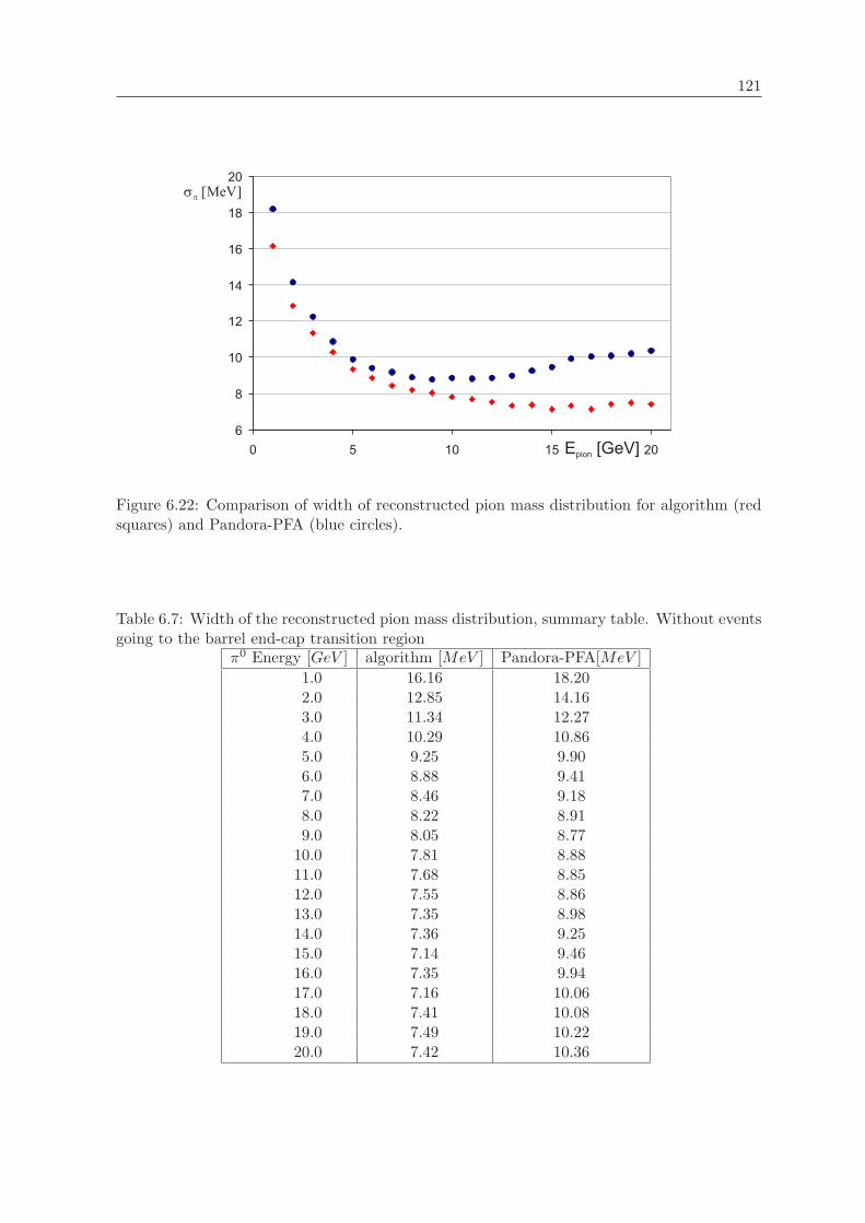
121
Figure 6.22: Comparison of width of reconstructed pion mass distribution for algorithm (redsquares) and Pandora-PFA (blue circles).
Table 6.7: Width of the reconstructed pion mass distribution, summary table. Without eventsgoing to the barrel end-cap transition region
π0 Energy [GeV ] algorithm [MeV ] Pandora-PFA[MeV ]1.0 16.16 18.202.0 12.85 14.163.0 11.34 12.274.0 10.29 10.865.0 9.25 9.906.0 8.88 9.417.0 8.46 9.188.0 8.22 8.919.0 8.05 8.77
10.0 7.81 8.8811.0 7.68 8.8512.0 7.55 8.8613.0 7.35 8.9814.0 7.36 9.2515.0 7.14 9.4616.0 7.35 9.9417.0 7.16 10.0618.0 7.41 10.0819.0 7.49 10.2220.0 7.42 10.36
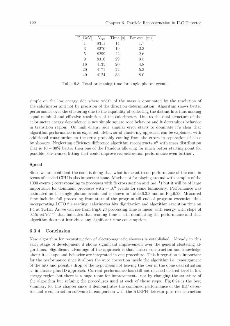
122 Chapter 6. Particle Reconstruction in ILC Detector
E [GeV] Nevt Time [s] Per evt. [ms]1 8311 14 1.73 8276 19 2.35 8299 22 2.69 8316 29 3.516 4135 20 4.820 4171 22 5.340 4124 33 8.0
Table 6.8: Total processing time for single photon events.
simple on the low energy side where width of the mass is dominated by the resolution ofthe calorimeter and not by precision of the direction determination. Algorithm shows betterperformance over the clustering due to the capability of collecting the distant hits thus makingequal nominal and effective resolution of the calorimeter. Due to the dual structure of thecalorimeter energy dependence is not simple square root behavior and it determines behaviorin transition region. On high energy side angular error starts to dominate it’s clear thatalgorithm performance is as expected. Behavior of clustering approach can be explained withadditional contribution to the error probably coming from the errors in separation of closeby showers. Neglecting efficiency difference algorithm reconstructs π0 with mass distributionthat is 10 − 30% better then one of the Pandora allowing for much better starting point forpossible constrained fitting that could improve reconstruction performance even further .
Speed
Since we are confident the code is doing that what is meant to do performance of the code interms of needed CPU is also important issue. Maybe not for playing around with samples of the1000 events ( corresponding to processes with fb cross section and 1ab−1) but it will be of largeimportance for dominant processes with ∼ 106 events for same luminosity. Performance wasestimated on the single photon events and is shown in Table.6.3.3 and on Fig.6.23. Measuredtime includes full processing from start of the program till end of program execution thusincorporating LCIO file reading, calorimeter hits digitization and algorithm execution time onP4 at 3GHz. As we can see from Fig.6.23 processing time is linear with energy with slope of0.15msGeV −1 that indicates that reading time is still dominating the performance and thatalgorithm does not introduce any significant time consumption.
6.3.4 Conclusion
New algorithm for reconstruction of electromagnetic showers is established. Already in thisearly stage of development it shows significant improvement over the general clustering al-gorithms. Significant advantage of the approach is that cluster construction and knowledgeabout it’s shape and behavior are integrated in one procedure. This integration is importantfor the performance since it allows the auto correction inside the algorithm i.e. reassignmentof the hits and possible drop of the hypothesis not leaving the user in the done deal situationas in cluster plus ID approach. Current performance has still not reached desired level in lowenergy region but there is a huge room for improvements, not by changing the structure ofthe algorithm but refining the procedures used at each of those steps. Fig.6.24 is the bestsummary for this chapter since it demonstrates the combined performance of the ILC detec-tor and reconstruction software in comparison with the ALEPH detector plus reconstruction

123
Figure 6.23: Speed of the algorithm per photon of given energy. Connected dots are datapoints form table 6.3.3, gray line represents linear fit.
0.8
1.0
Figure 6.24: π0 reconstruction efficiency for ALEPH (black circles) and ILC detector withproposed algorithm (red dots).
[122] for π0. I hope that this picture will bring us at least a permill closer to having the realdetector.


Chapter 7
Summary and conclusions
The title of the theses is: ”Measurement of quartic couplings at ILC and study of novel particleflow algorithms”. What I want to stress is that altho large work has been done this thesesis not presenting measurement at ILC. It presents results for given set of ILC machine anddetector parameters that were considered as realistic at one point in time. Basic assumptionsfor the measurement of quartic couplings are:
• Both electron and positron polarizations are available
• Collected luminosity is at least 1ab−1 at highest reachable energy (1TeV)
• Jet energy resolution is 30%/√E
• Hermeticity and tracker coverage is as supposed for the TESLA TDR detector
• SM cross sections are calculated with precision at the percent level
Accepting those assumptions, and fighting that they do not stay only assumptions, it ispossible to say that :
• direct measurement of quartic couplings to the theoretically favored precision (∼ 1) ispossible (if isospin conservation is assumed)
• Under equal time sharing between e+e− and e−e− channels weak boson scattering pro-cesses are giving equivalent results (if isospin conservation is assumed).
• Prospects for large indirect reach from this measurement are bleak even under mostfavorable conditions, specially in scalar and vector channel.
• If one accepts assumptions stated above as realistic one the precision is limited only withstatistics.
Jet energy resolution goal is mostly driven with weak boson scattering processes, so we havestudied in some details what are the contributions to the final performance and how it canbe reached. On of the major ingredients in acheaving this goal is accurate separation ofthe showers in ECAL. New approach to reconstruction in ECAL, that fully exploits powerof the calorimeter designed for particle flow was presented. It shows superior performance(with efficiency above 99% ) in the EM shower energy range from 0.5-40GeV with no energydependence of the performance, with possible further improvements it refreshes the hope toreach desired performance.
125

Appendix A
Theory addons
Notation
Gamma matricesγ0 =
(0 11 0
)(A.1)
γi =( 0 −σiσi 0
)(A.2)
γ5 = iγ0γ1γ2γ3 =(
1 00 −1
)(A.3)
γ†5 = γ5 (γ5)2 = I {γ5, γi} = 0 (A.4)
projection operators
PR =1 + γ5
2and PL =
1− γ5
2(A.5)
ψL = (Lψ)†γ0 = ψ†L†γ0 = ψ†γ0R = ψR (A.6)
ψR = ψL (A.7)
Fermion mass term mixes right- and left-handed fermion components,
ψψ = ψRψL + ψLψR (A.8)
Pauli matricesτ1 =
(0 11 0
)τ2 =
(0 −ii 0
)τ3 =
(1 00 −1
)(A.9)
with commutation relations[τi, τj ] = i εijk τk (A.10)
Lepton number conservation - neutrino masses equal 0 ! parity violation (pseudo scalarJipe)
∂µ ≡ ∂
∂xµ≡ ( ∂
∂x0,∇)
(A.11)
∂µ ≡ ∂
∂xµ≡ ( ∂
∂x0,−∇)
(A.12)
126
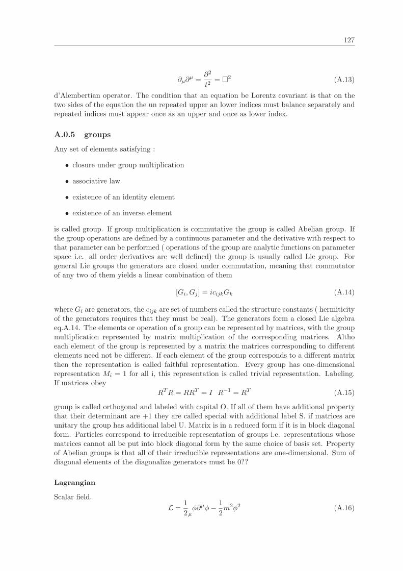
127
∂µ∂µ =
∂2
t2= ¤2 (A.13)
d’Alembertian operator. The condition that an equation be Lorentz covariant is that on thetwo sides of the equation the un repeated upper an lower indices must balance separately andrepeated indices must appear once as an upper and once as lower index.
A.0.5 groups
Any set of elements satisfying :
• closure under group multiplication
• associative law
• existence of an identity element
• existence of an inverse element
is called group. If group multiplication is commutative the group is called Abelian group. Ifthe group operations are defined by a continuous parameter and the derivative with respect tothat parameter can be performed ( operations of the group are analytic functions on parameterspace i.e. all order derivatives are well defined) the group is usually called Lie group. Forgeneral Lie groups the generators are closed under commutation, meaning that commutatorof any two of them yields a linear combination of them
[Gi, Gj ] = icijkGk (A.14)
where Gi are generators, the cijk are set of numbers called the structure constants ( hermiticityof the generators requires that they must be real). The generators form a closed Lie algebraeq.A.14. The elements or operation of a group can be represented by matrices, with the groupmultiplication represented by matrix multiplication of the corresponding matrices. Althoeach element of the group is represented by a matrix the matrices corresponding to differentelements need not be different. If each element of the group corresponds to a different matrixthen the representation is called faithful representation. Every group has one-dimensionalrepresentation Mi = 1 for all i, this representation is called trivial representation. Labeling.If matrices obey
RTR = RRT = I R−1 = RT (A.15)
group is called orthogonal and labeled with capital O. If all of them have additional propertythat their determinant are +1 they are called special with additional label S. if matrices areunitary the group has additional label U. Matrix is in a reduced form if it is in block diagonalform. Particles correspond to irreducible representation of groups i.e. representations whosematrices cannot all be put into block diagonal form by the same choice of basis set. Propertyof Abelian groups is that all of their irreducible representations are one-dimensional. Sum ofdiagonal elements of the diagonalize generators must be 0??
Lagrangian
Scalar field.L =
12µφ∂µφ− 1
2m2φ2 (A.16)

128 Chapter A. Theory addons
leads to(¤2 +m2)φ = 0 (A.17)
Spin 1/2 field .L = iψγµ∂µψ −mψψ (A.18)
(iγµ∂µ −m)ψ = 0 (A.19)
Massless vector fieldL = −1
4FµνF
µν − jµAµ (A.20)
Noether’s theorem
Fundamental result that has connected symmetry and interaction is the Neoether’s theorem[27]. If an action is invariant under some group of transformations (symmetry), then thereexist one or more conserved quantities (constants of motion) which are associated to thesetransformations. Let us assume that Lagrangian of the physical system is invariant undersome set of continuous transformations
φi(x) → φ′i(x) = φi(x) + εδiφi(x) +O(ε2) (A.21)
i.e.L[φi(x), ∂µφi(x)] = L[φ′i(x), ∂µφ
′i(x)] (A.22)
leads toδεL = 0 =
∑
i
([∂L∂φi
− ∂µ(∂L
∂(∂µφi))]δεφi + ∂µ[
∂L∂(∂µφi)
δεφi])
(A.23)
If the fields satisfy Euler-Lagrange equations of motion
∂L∂φi
− ∂µ[ ∂L∂(∂µφi)
]= 0 (A.24)
the first term in eq.A.23 is zero, therfore system have conserved current
Jµ ≡∑
i
∂L∂(∂µφi)
δεφi and ∂µJµ = 0 (A.25)
That allowed to construct a conserved charge
Q ≡∫d3xJ 0 (A.26)
In this way logical direction from symmetries to conservation laws thus selection rulesobserved in the nature correspond to th dynamical symmetries of the Lagrangian.
A.0.6 Goldston theorem
When an exact continous global symmetry is spontaneously broken, i.e. it is not a symmetry ofthe physical vacuum, the theory contains one massless scalar particle for each broken generatorof the original symmetry group. Let us consider a Lagrangian of NG real scalar fields φ,belonging to a NG dimensional vector Φ,
L =12∂µΦ∂µΦ− V (Φ) (A.27)

129
Suppose that G is a contionous group that lets the Lagrangian invariant and that Φtransforms like
δΦ = −iαaT aΦ (A.28)
Since the potential is invariant uder G, we have
δV (Φ) =∂V (Φ)∂φi
δφi = −i∂V (Φ)∂φi
αa(T a
)ijφj = 0 (A.29)
Gauge parameters αa are arbitrary ( and nonzero), and we have NG eqations
∂V (Φ)∂φi
αa(T a
)ijφj = 0 (A.30)
for a = 1, . . . , NG. Taking another derivative of eq.A.30, we obtain
∂2V (Φ)∂φk∂φi
(T a
)ijφj +
∂V (Φ)∂φi
(T a
)ik
= 0 (A.31)
If we evaluate this result at the vacuum state Φ = Φ0, which minimizes the potential, weget
∂2V (Φ)∂φk∂φi
∣∣∣∣∣Φ=Φ0
(T a
)ijφ0j = 0 (A.32)
or in terms of mass matrix,M2ki
(T a
)ijφ0j = 0 (A.33)
If, after we choose a ground stata, sub-group g of G, with dimension ng, remains symmetryof the vacuum, then for each generator of g
(T a
)ijφ0j = 0 for a = 1, , ng < NG (A.34)
while for the (NG − ng) generators that break the symmetry,(T a
)ijφ0j 6= 0 for a = ng + 1, , NG (A.35)
Taking into account eq.A.33 it is clear that there are (NG − ng) zero eigenalues of the massmatrix i.e. massless Goldston bosons.

Appendix B
Pflow factorization
This chapter contains results for e+e−Z,W+W−, tt at center of mass energy 500GeV in tablesB.1,B.2,B.3 and 1TeV in tables B.4,B.5,B.6. Generation of events is done by Pythia withfollowing flags:
MSTJ(22) = 3PARJ(72) = 300.0D0 (B.1)
that are forcing decay of all unstable particles to the sphere with radius 300mm around IP. Asalredy mentioned only hadronic decay channels were considered by turning of leptonic decaychannels by setting MDME(i,1) = 0 ; where i = {206, 207, 208} for W , and i = {182, ..., 187}for Z. Initial state radiation is turned off with:
MSTP (61) = 0MSTP (11) = 0 (B.2)
Exclusive tt production is regulated with opening or closing chnanels γ → tt (mdme(167,1))and Z → tt (mdme(167,1)). Generated subprocesses are Z production msub(1) and W pairproduciton msub(25). Conditions under which results in the table are extracted are explainedin 5.1.3. For 1TeV effect of mass assignment is shown combined.
Effect σ[GeV ]separate σ[GeV ]joined σ[GeV ]total (%/√E) σ% of total
Eν 0.75 0.75 0.75 (3.35) 2.44θ◦ < 5 1.80 1.95 1.95 (8.72) 14.03Pt < 0.36GeV 1.96 2.76 2.76 (12.36) 16.63σHCAL 3.04 3.04 4.11 (18.38) 40.01σECAL 2.20 3.75 4.66 (20.84) 20.95Mneutral 1.03 3.89 4.77 (21.35) 4.59Mcharged 0.56 3.94 4.81 (21.49) 1.36
Table B.1: Contributions to the width of reconstructed mass distribution from different sourcesfor qq events at 500GeV. Column joined means that PFA and non PFA contributions weresummed sequentially. Total means that all the contributions were summed. In last columpartial contribution of each effect to the total width is expressed in percent.
130
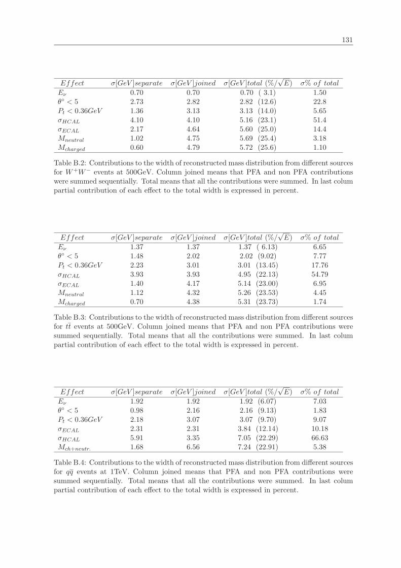
131
Effect σ[GeV ]separate σ[GeV ]joined σ[GeV ]total (%/√E) σ% of total
Eν 0.70 0.70 0.70 ( 3.1) 1.50θ◦ < 5 2.73 2.82 2.82 (12.6) 22.8Pt < 0.36GeV 1.36 3.13 3.13 (14.0) 5.65σHCAL 4.10 4.10 5.16 (23.1) 51.4σECAL 2.17 4.64 5.60 (25.0) 14.4Mneutral 1.02 4.75 5.69 (25.4) 3.18Mcharged 0.60 4.79 5.72 (25.6) 1.10
Table B.2: Contributions to the width of reconstructed mass distribution from different sourcesfor W+W− events at 500GeV. Column joined means that PFA and non PFA contributionswere summed sequentially. Total means that all the contributions were summed. In last columpartial contribution of each effect to the total width is expressed in percent.
Effect σ[GeV ]separate σ[GeV ]joined σ[GeV ]total (%/√E) σ% of total
Eν 1.37 1.37 1.37 ( 6.13) 6.65θ◦ < 5 1.48 2.02 2.02 (9.02) 7.77Pt < 0.36GeV 2.23 3.01 3.01 (13.45) 17.76σHCAL 3.93 3.93 4.95 (22.13) 54.79σECAL 1.40 4.17 5.14 (23.00) 6.95Mneutral 1.12 4.32 5.26 (23.53) 4.45Mcharged 0.70 4.38 5.31 (23.73) 1.74
Table B.3: Contributions to the width of reconstructed mass distribution from different sourcesfor tt events at 500GeV. Column joined means that PFA and non PFA contributions weresummed sequentially. Total means that all the contributions were summed. In last columpartial contribution of each effect to the total width is expressed in percent.
Effect σ[GeV ]separate σ[GeV ]joined σ[GeV ]total (%/√E) σ% of total
Eν 1.92 1.92 1.92 (6.07) 7.03θ◦ < 5 0.98 2.16 2.16 (9.13) 1.83Pt < 0.36GeV 2.18 3.07 3.07 (9.70) 9.07σECAL 2.31 2.31 3.84 (12.14) 10.18σHCAL 5.91 3.35 7.05 (22.29) 66.63Mch+neutr. 1.68 6.56 7.24 (22.91) 5.38
Table B.4: Contributions to the width of reconstructed mass distribution from different sourcesfor qq events at 1TeV. Column joined means that PFA and non PFA contributions weresummed sequentially. Total means that all the contributions were summed. In last columpartial contribution of each effect to the total width is expressed in percent.

132 Chapter B. Pflow factorization
Effect σ[GeV ]separate σ[GeV ]joined σ[GeV ]total (%/√E) σ% of total
Eν 1.93 1.93 1.93 (6.10) 5.41θ◦ < 5 4.14 4.57 4.57 (14.44) 24.88Pt < 0.36GeV 2.50 5.21 5.21 (16.48) 9.07σECAL 1.84 1.84 5.53 (17.47) 4.91σHCAL 5.82 3.03 8.03 (25.38) 49.17Mch+neutr. 2.10 6.46 8.30 (26.23) 6.40
Table B.5: Contributions to the width of reconstructed mass distribution from different sourcesfor W+W− events at 1TeV. Column joined means that PFA and non PFA contributions weresummed sequentially. Total means that all the contributions were summed. In last columpartial contribution of each effect to the total width is expressed in percent.
Effect σ[GeV ]separate σ[GeV ]joined σ[GeV ]total (%/√E) σ% of total
Eν 4.17 4.17 4.17 (13.19) 21.18θ◦ < 5 3.13 5.21 5.21 (16.49) 11.94Pt < 0.36GeV 3.81 6.46 6.46 (20.43) 17.68σECAL 1.97 1.97 6.75 (21.36) 4.73σHCAL 5.87 3.12 8.95 (28.30) 41.98Mch+neutr. 1.41 6.56 9.06 (28.65) 2.42
Table B.6: Contributions to the width of reconstructed mass distribution from different sourcesfor tt events at 1TeV. Column joined means that PFA and non PFA contributions were summedsequentially. Total means that all the contributions were summed. In last colum partialcontribution of each effect to the total width is expressed in percent.

Appendix C
Summary of the formulae forphoton shower parameterization
C.1 Homogeneous media
C.1.1 Average longitudinal profiles
Thom = ln y − 0.858 (C.1)
αhom = 0.21 + (0.492 + 2.38/Z) ln y (C.2)
C.1.2 Average radial profiles
RC,hom(τ) = z1 + z2τ (C.3)
RT,hom(τ) = k1
(exp(k3(τ − k2)) + exp(k4(τ − k2))
)(C.4)
phom(τ) = p1 exp(p2 − τ
p3− exp(
p2 − τ
p3))
(C.5)
z1 = 0.0251 + 0.00319 lnEz2 = 0.1162− 0.000381Zk1 = 0.659− 0.00309Zk2 = 0.645k3 = −2.59 (C.6)k4 = 0.3585 + 0.0421 lnEp1 = 0.401− 0.00094Zp2 = 0.401 + 0.00187Zp3 = 1.313− 0.0686 lnE
133
134 Bibliography
C.2 Sampling calorimeter
C.2.1 Material and geometry parameters
ωi =ρidi∑j ρjdj
Zeff =∑
i
ωiZi
Aeff =∑
i
ωiAi
1X0,eff
=∑
i
ωiX0,i
1RM,eff
=1Es
∑
i
ωiEc,iX0,i
(Es = 21.2MeV ) (C.7)
Ec,eff = X0,eff
∑
i
ωiEc,iX0,i
FS =X0,eff
da + dp
e =1
1 + 0.0007(Zp − Za)
C.2.2 Average longitudinal profiles
Tsam = Thom − 0.59F−1S − 0.53(1− e) (C.8)
αsam = αhom − 0.444F−1S (C.9)
C.2.3 Average radial profiles
RC,sam = RC,hom − 0.0203(1− e) + 0.00397F−1S exp(−τ) (C.10)
RT,sam = RT,hom − 0.14(1− e)− 0.495F−1S exp(−τ) (C.11)
psam = phom + (1 + e)(0.348− 0.642F−1S exp(−(τ − 1)2)) (C.12)
Bibliography
[1] M.Battaglia, The International Linear Collider, hep-ex:0705.3997v1 , 28.05.2007
[2] Parameters Subcommittee of the International Linear Collider Steering Committee,Parameters for the Linear Collider 30.09.2003.
[3] Parameters Subcommittee of the International Linear Collider Steering Committee,Parameters for the Linear Collider, 20.11.2006.
[4] ITRP Recomendation, September 2004.http://www.fnal.gov/directorate/icfa/ITRP Report Final.pdf
[5] ILC Global Desing Effort and World Wide Study, “International Linear Collider ReferenceDesign Report”, August 2007.
[6] T.Behnke et al.“TESLA: The superconducting electron positron linear collider withan integrated X-ray laser laboratory. Technical design report. Part 4. A Detector forTESLA”,DESY-01-011
[7] T.Behnke, G.Blair, K.Monig and M.Pohl, BRAHMS Version 1.00 aMonte Carlo Program for Detector at a 800GeV Linar Collider (1998),http://www.hep.ph.rhbnc.ac.uk/blair/detsim/brahms.html
[8] Detector Outline Document for Large Detector Concept, final version, july 2006. Preparedby the LDC group for the Reference Design Report of the International Linear Collider.http://www.ilcldc.org/
[9] MOKKA: a GEANT4 based full detector simulation for the ILDC.http://polwww.in2p3.fr/MOKKA
[10] The SiD concept group, T.Abe at al. SiD Detector Outline Documenthttp://hepuchicago.edu/ oreglia/documents/dod
[11] GLD Concept Study Group, “GLD Detector Outline Document” arXiv:physics/0607154
[12] F.Sauli, “GEM: A new concept for electron amplification in gas detectors”, Nuclear In-struments and Methods A 386, p531 1997.
[13] Y.Giomataris, P.Rebourgaerd, J.P.Robert and G.Charpak, “MICROMEGAS: A high-granularity position-sensitive gasous detector for high particle-flux environments, NuclearInstruments and Methods A 376 (1996) 29.
[14] T.Behnke et al. Track Reconstruction Efficency, LC note LC-DET 2007-029.
[15] Jean-Claud Brient,Advantages and drawbacks for Silicon based ECAL, Snowmass 2005
135

136 Bibliography
[16] P.Krstonosic, Track to DOD detector, presented at ECFA software and Physics simulationmeeting 16.08.06
[17] M.Picollo private comunication.
[18] A.Stahl,K.Bußer, LC-DET-2004-034.
[19] H.Vidou, presentation at LDC meeting , Wienna 2005.
[20] ILC Global Design Effort and World Wide Study Groups, International Linear ColliderReference Design Report Volume 4 Detector,august 2007.
[21] G.Kane, Modern Elementary Particle Physics, Addison-Wesley 1987.
[22] W.E.Burcham M.Jobes, Nuclear and Particle Physics, Longman Scientific Technical1994.
[23] S.F.Novaes, Standard Model: An Introduction, hep-ph/0001283v1
[24] W.Buchm”uller, C.L”udeling, Field Theory and Standard Model, hep-ph609184v1
[25] A.Pich, The Standard Model of Electroweak Interacions, hep-ph7054264v1
[26] A. Salam , J.C. Ward , Phys.Lett. 13, 168 (1964)
[27] http://arxive.org/pdf/physics/0503066
[28] J.Goldstone, Nuouvo Cim. 19, 154 (1961)
[29] Y.Nambu , Phys.Rev.Lett 4, 380(162)
[30] W. Pauli , Open Letter to all radioactive persons 1930, English translation, Physics Today31, 27(1978)
[31] W. Pauli , Septieme Consiel de Physique, Solvay (Gauthier-Villars Paris 1934) p.324
[32] E.Fermi Z.Phys. 88,161(1934) , Nuovo Cim 11,1(1934)
[33] G.Gamow and E.Teller Phys.Rev. 49, 895(1936)
[34] B.Pontecorvo Phys.Rev. 72, 246(1947)
[35] W. Heisenberg , Z.Physics 77, 1 (1932)
[36] R. Utiyama , Phys. Rev. 101, 1597 (1956)
[37] J.Schwinger, Ann. Phys. 2, 407 (1957)
[38] R.P. Feynmann , M. Gell-Mann , Phys.Rev. 109, 193 (1958)
[39] R.E. Marshak, E.C.G. Sudarshan, Phys.Rev 109, 1860 (1958)
[40] J.J. Sakurai, Nuovo Cim. 7, 649 (1958)
[41] S.A. Bludmann , Nuovo Cim. 9, 433 (1958)
[42] J. Leite Lopes , Nucl. Phys. 8, 234 (1958)
[43] S.L. Glashow , Nucl.Phys. 22, 579(1961)

137
[44] S.Weinberg , Phys.Rev.Lett. 19, 1264(1967)
[45] A.Salam , “Elementary Particle Theory”,The Nobel Symposium no 8, Almqvist andWiksell, Stockholm 1968, p367.
[46] G.’t Hooft , Nucl. Phys. B33, 173 (1971) and B35 , 167 (1971)
[47] C.S. Wu, E. Ambler, R.W. Haywood, D.D. Hoppes and R.P. Hudson, Phys. Rev.105,1413(1957)
[48] M. Goldhaber, L. Grodzins and A.W. Sunayr, Phys. Rev. 109, 1015(1958)
[49] R.L. Garwin, L.M. Lederman and M. Weinrich, Phys.Rev. 105, 1415(1957)
[50] M.T. Burgy, V.E. Krohn, T.B. Novey, G.R. Ringo and V.A. Telegdi, Phys. Rev. 110,1214(1958)
[51] S.S. Gerstein and Ya.B. Zel’dovitch, Soviet Phys JETP 2, 579 (1956)
[52] C.P Burgess and D. London, Phys.Rev. D 48, 4337(1993)
[53] E.S. Abers and B.W.Lee, Phys.Rep. 9, 1(1973)
[54] W. Kilian , Electroweak Symmetry Breaking The Bottom-Up Approach, Springer, 2003.
[55] A. Dobado, A.Gomez-Nicola, A.L.Maroto and J.R.Pelaez, Effective Lagrangians for Stan-dard Model, Springer 1997.
[56] P.W. Higgs, Phys. Lett. 12, 132(1964)
[57] F.Englert and R.Brout, Phys.Rev.Lett 13, 321(1964)
[58] G.S. Guralnik, C.R.Hagen and T.W.B.Kibble, Phys.Rev.Lett 13, 585(1964)
[59] G.Moortgat-Pick et. al, The role of polarized positrons and electrons in revealing funda-mental interacitons at the Linear Collider, DESY 05-059
[60] S.Wolfram , Mathematica book, Cambridge University press
[61] W.Kilian, WHIZARD 1.26,A generic Monte Carlo integration and event generation pack-age for multi-particle processes,LC-TOOL-2001-039 ,2001
[62] T.Ohl, O’Mega: An Optimizing Matrix Element Generator, Proceedings of the Workshopon Advanced Computing and Analysis Technics in Physics Research, Fermilab, October2000, IKDA 2000/30, hep-ph/0011243
[63] M.Pohl, H.J.Schreiber, SIMDET V4.,A parametric Monte Calro for a TESLA Detector,DESY 02-061,May 2002
[64] F.James, MINUIT Function Minimization and Error Analysis, Version 94.1, CERN Pro-gram Library Long Writeup D506
[65] M.Duda, Studien zur Systematik der W-Massen-Bestimmung, diplomarbeit, RWTHAachen, December 2003
[66] J.P. Ochoa Ricoux, Optimal Pairing algorithm for 4 and 5 jet events at lep. L3 Note 2786,31.10.2002
138 Bibliography
[67] S.Moretti,L.Lonnblad, T.Sjostrand , New and Old Jet Clustering Algorithms for Electron-Positron Events hep-ph 9804296v1
[68] S.M.X. Hansen, D.J.Jackson, R.Hawkings and C.J.S.Damerell, Flavour Tagging Studiesfor the TESLA Linear Collider, LC-PHSM-2001-024, 2001 http://www.desy.de/~lcnotes
[69] T.Kuhl private communicaiton
[70] D.J.Jackson, A topological vertex reconstruction algorithm for hadronic jets, SLAC-PUB-7215, December 1996
[71] T. Sjostrand, P. Eden, C. Friberg, L. Lonnblad, G. Miu, S. Mrenna and E. Nor-rbin,PYTHIA V6.221, Computer Physics Commun. 135 (2001) 238
[72] E.Kouznetsova A.Drugakov private communicaiton.
[73] W.Menges, A sudy of charged current triple gauge couplings at TESLA, LC-PHSM-2001-022
[74] J.Sekaric, Studies of Gauge Boson Production with a γγ-Collider at TESLA, DESY-THESES-2005-042
[75] Lucas Tailor ,”Perfromance of the L3 Detector” L3Note 2132, july 1997
[76] O.Adriani et al.”Hadron Calorimetry in L3” , Nuclear Instruments and Methods inPhysics Research A 302 , 53=62 (1991)
[77] Satoshi Mihara and Satoru Yamashita, “MT 3.00 a new algorithm to calculate energyflow base on MT package”, OPAL TN575 november 1998
[78] V.Morgunov, Calorimeter Energy Calibration usign the energy conservation law. LCWS2006.
[79] C.Castanier, P.Gay, P.Lutz and J.Orloff. Higgs selfcoupling measurment in e+e- collisionsat center-of-mass energy of 500GeV. hep-ex/0101028, 2001.
[80] T.Barlkow, Higgs Self Coupling Errors Versus Jet Energy Resolu-tion,presented at Silicon Detector Workshow October 26-28, 2006.http://www.slac.stanford.edu/~timb/sid/slac oct 2006/hhz.pdf
[81] T.Barklow, Physics Impact of Detector Performance,presented at LCWS , 2005http://www-conf.slac.stanford.edu/lcws05/program/talk/18mar2005.ppt
[82] J.C.Brient, Measurement of the Higgs decay into WW ∗ at future e+e- linear colliders.LC-PHSM-2004-002 http://www.desy.de/~lcnotes .
[83] M.Kobel, R.Chierici, S.Rosati. Strong electroweak symmetry breaking signals in WWscattering at TESLA. LC-PHSM-2001-038 http://www.desy.de/~lcnotes .
[84] A.Raspereza, LCWS2006 Workshop, march 2006
[85] S.Magill,S.Kuhlman , LC HCAL Absorber (SS vs W) and P-Flow Perfor-mance (Scintillator vs RPC) Comparisons, LCWS05,17 March 2005 http://www-conf.slac.stanford.edu/lcsim05/lcws05 talks/050321/Magill.pdf

139
[86] S.Yamamoto, Status of PFA study Jet Energy Resolution Studies using CheatedPFA, GLD meeting , 25 May 2005 http://ilcphys.kek.jp/meeting/lcdds/archives/2005-05-25/20050525GLDmeeting.pdf
[87] R.Casell, Angular dependence of digital RPC HCAL responce to neutral hadrons,13.10.2005
[88] TESLA TDR, part IV , page IV-71
[89] F.Gaede, T.Behnke, N.Graf and T.Johnson “LCIO- Persitensy framework for linear col-lider simulation studies”, LC-TOOL-2003-053 or arXiv:physics/0306114v1
[90] P.M.S. Blackett and G.P.S Occhianlini, Proc.R.Soc. A 139, 609 (1933)
[91] P.M.S. Blackett, G.P.S Occhianlini and J.Chadwick Proc.R.Soc. A 144, 235 (1933)
[92] J.H.Bhabha and W.Heitler, Proc.R.Soc. A 159, 432 (1936)
[93] J.F.Carlson and J.R. Oppenheimer, Phys.Rev. 51, 220 (1936)
[94] B.Rossi and K.Greisen, Rev.Mod.Phys. 13, 240 (1941)
[95] I.Tamm and S.Belenky, Phys.Rev. 70, 660 (1946)
[96] W.R. Leo, Techniques for Nuclear and Particle Physics Experiments, Springer, New York
[97] W.M.Yoo,et al. Reivew of Particle Physics (chapter Passage of particles through matter),Journal of Physics G33, 1 (2006)
[98] C.Leroy and P.G. Rancoita, Rep.Prog.Phys. 63, 505 (2000)
[99] Y.S.Tsai Rev.Mod.Phys. 46, 815 (1974)
[100] R.Wigmans nad M.T.Zeyrek, NIM A485, 385(2002)
[101] R.L.Ford W.R.Nelson The EGS code system: computer program for the MOnte calrosimulation of electromagnetic cascade showers (version 3) , SLAC Report SLAC-210, 1978.
[102] W.R.Nelson, H.Hiriyama and D.W.O Rogers, The EGS4 code system, SLAC-265 1985.
[103] H.Hirayama et al. The EGS5 Code System, Stanford Linear Accelerator Center ReportSLAC-R-730, 2005
[104] W.R. Nelson, C. Field Comparison of EGS5 simulaitons with experiment NIM A 572,1083 (2007)
[105] B.Rossi, High Energy Particles, Prentice Hall inc. 1952
[106] M.J.Berger and S.M.Seltzer, “Tables of Energy Losses and Ranges of Electrons andPositrons”, NASA Report ,NASA-SP-2012, 1964
[107] E.Longo nad I.Sestili, NIM 128, 283(1975)
[108] W.R.Nelson, T.M.Jenkins, R.C.McCall and J.K.Cobb, Phys.Rev. 149, 201(1966)
[109] G.Bathow et al., Nucl. Phys. B20, 592 (1970)

140 Bibliography
[110] Walter R. Nelson, Theodore M. Jenkins, Richard C. McCall, and Joseph K. Cobb ,“Electron-Induced Cascade Showers in Copper and Lead at 1 GeV”, Phys. Rev. 149, 201- 208 (1966)
[111] G. Bathow et al.,”Measurement of the longitudinal and lateral development of electro-magnetic cascades in lead, copper and aluminum at 6GeV”, Nuclear Physics B 20 , 592(1970)
[112] G.Ferri et al. (SICAPO Collaboration), NIM A 273,
[113] G. Grindhammer and S.Peters, “The Parametrized Simulation of ElectromagneticShower in Homogeneous and Sampling Calorimeters” , arXiv:hep-ex/0001020v1
[114] J.Weng, E.Barberio and A.Waugh, “Fast shower parametrization for electromagneticcascades”, November 2005.
[115] D.Mount and S.Arya, ANN: Approximate Nearest Neighbors (library) v 1.1 ,http://www.cs.umd.edu/~mount/ANN
[116] M.Thomson, Progress with Particle Flow Calorimetry, arXiv: pysics.ins-det 0607261v1and 0709.1360v1
[117] PandoraPFA , http://www.hep.by.cam.ac.uk~thomson/pandoraPFA
[118] Mathematica4 and Mathematica5 , http://www.wolfram.com
[119] Y.Pei, Photon Identificaiton usign a Neural Network , L3 note 1564, 1994
[120] G.W.Wilson, Updates on Photon ID using a Longitudianl H-Matrix, 03.04.2007
[121] G.W.Wilson, Impact of π0 Reconstruction on PFA and Neutral hadron TOF possibili-ties. LCWS07
[122] D.Buskulic at al. Performance of the ALEPH detector at LEP, Nuclear Instruments andMethods in Physics Research A 360, 481-506 (1995)
[123] P.Abreu at al. Performance of the DELPHI detector , Nuclear Instruments and Methodsin Physics Research A 378, 57-100 (1996)