measurement of mixing characteristics of the … of mixing characteristics of the missouri river...

Measurement of Mixing Characteristics of the Missouri River Between Sioux City, Iowa, and Plattsmouth, Nebraska

GEOLOGICAL SURVEY WATER-SUPPLY PAPER 1899-G

Measurement of Mixing Characteristics of the Missouri River Between Sioux City, Iowa, and Plattsmouth, NebraskaBy NOBUHIRO YOTSUKURA, HUGO B. FISCHER, and WILLIAM W. SAYRE

CONTRIBUTIONS TO THE HYDROLOGY OF THE UNITED STATES

GEOLOGICAL SURVEY WATER-SUPPLY PAPER 1899-G

Measurement of longitudinal dispersion, transverse mixing, channel geometry, and transverse velocity distribution

UNITED STATES GOVERNMENT PRINTING OFFICE, WASHINGTON : 1970

UNITED STATES DEPARTMENT OF THE INTERIOR

WALTER J. HICKEL, Secretary

GEOLOGICAL SURVEY

William T. Pecora, Director

For sale by the Superintendent of Documents, U.S. Government Printing Office Washington, D.G. 20402 - Price 25 cents (paper cover)

CONTENTSPage

Symbols..__-_--__-___-___-__-_----_____-_________________________ ivAbstract- ________________________________________________________ GlIntroduction, _____________________________________________________ 1

Acknowledgments-____---_-_--__--__--____-__-___-____________ 3Longitudinal dispersion.___________________________________________ 3

Description of the test reach.___________________________________ 3Test procedure.__-___--__-_____--__-_-_-__--__________________ 5Data-.____-___-_--___--_-_-__-__--_--____________________ 6Computation of the longitudinal dispersion coefficient-_____________ 8

Routing procedure-__-___-_-___--______-__-__--_-_________ 8Method of moments.______________________________________ 10

Transverse mixing.._______________________________________________ 11Description of the test reach.____________________________________ 11Test procedure.__-_-___-_____-_-___---_-_-_-__-__-_______-_-__ 13Data---_--_---_---_-___-_-_--__-___-__-_--____________-_-. 18Computation of the transverse mixing coefficient-_________________ 20

Method of moments.______________________________________ 20Computer simulation method.--__-____-_-_-_______-________ 21

Summary and conclusions._________________________________________ 27References-____________--___-___-_-----_----_---_--__-__-___-____ 29

ILLUSTRATIONSPage

FIGURE 1. Map of study reach, Missouri River between Sioux City,Iowa, and Plattsmouth, Nebr_______________________ G4

2. Graph showing longitudinal dispersion on the Missouri River comparison of the November 1967 data with the October 1966 data________-__-__--__-_-________ 7

3. Graph showing measured mean time of passage and vari ance as functions of distance.______-___-___-_-____-_ 12

4. Sketch showing reach of the Missouri River for thetransverse mixing test-_____________________________ 14

5. Graph showing observed transverse profiles of velocity and depth at cross sections not affected by bridge abutments._______________________________________ 15

6. Photograph showing mixing of dye immediately down stream from injection site at Blair Highway Bridge____ 16

7. Sketch illustrating method for locating lateral samplingpositions.__________-____________--_____--__-__--_ 17

8-10. Graphs:8. Variance of transverse tracer distribution, ob

served and calculated__-______-_-_-_---_--- 219. Comparison of observed and calculated transverse

distribution of dye concentration at nine cross sections. ______________-__-_-___-__-_----- 25

10. Influence of E2 on transverse distribution of dyeconcentration._ __________-___-__----_-_--_ 26

TABLES

PageTABLE 1. Distribution of cross-sectional average dye concentration

with time, longitudinal dispersion test on the Missouri River, November 1967_____________________________ G6

2. Hydraulic data, longitudinal dispersion test on the Mis souri River, November 1967________________________ 8

3. Time-of-travel data, longitudinal dispersion test on theMissouri River, November 1967___--____--__________ 9

4. Dispersion coefficients by the routing procedure, longi tudinal dispersion test on the Missouri River, November 1967________-_________--_-____-______-___--_____- 10

5. Dispersion coefficients by the method of moments, longi tudinal dispersion test on the Missouri River, November 1967___-____-_____-_--__-_____-______--____--___- 13

6. Distribution of dye concentration in transverse direction, transverse mixing test on the Missouri River, Novem ber 17, 1967______--_____---_________-____-----___ 18

SYMBOLS

A Cross-sectional flow areaa s Dividing area between adjacent stream tubesC Cross-sectional mean tracer concentrationc Local tracer concentrationD Longitudinal dispersion coefficientd Mean flow depthEz Transverse mixing coefficientg Acceleration of gravityk Constant of transverse mixing coefficient1 Characteristic lengthM Mass flux of tracer per unit timeq Discharge in a stream tubeQ DischargeRR Recovery ratios Mean energy slopeT Lagrangian time scalet Time measured from the instant of injectiont' Dimensionless time scalet Mean time of passage for tracer cloud~t' Dimensionless mean time of passage for tracer cloudU Mean tracer velocity (mean flow velocity)U* Shear velocityu Local velocityV0 VolumeW Surface widthx Longitudinal distance measured from injection siteAx Increment of longitudinal distance2 Transverse distance from a boundaryAz Transverse distance between centroids of adjacent stream tubescr2 t Variance of longitudinal tracer distributioncr2 2 Variance of transverse tracer distribution

CONTRIBUTIONS TO THE HYDROLOGY OF THE UNITED STATES

MIXING CHARACTERISTICS OF THE MISSOURI RIVER BETWEEN SIOUX CITY, IOWA, AND PLATTSMOUTH, NEBRASKA

By NOBUHIRO YOTSUKURA, HucoB. FISCHER, and WIILLIAM W. SAYRE

ABSTRACT

Measurements of longitudinal dispersion, transverse mixing, channel geometry, and transverse velocity distribution were made in the Missouri River at a flow of about 33,000 cubic feet per second. The results show that the longitudinal dispersion coefficient for the 141-mile reach from Sioux City, Iowa, to Platts- mouth, Nebr., is about 16,000 square feet per second (approximately 5,600 U*d, where U* is the shear velocity and d is mean depth). The transverse mixing coefficient, Ez , for a 6-mile reach immediately downstream from Blair, Nebr., is about 1.3 square feet per second (approximately 0.6 U*d). The value of the longitudinal dispersion coefficient is one of the largest ever measured, rnd the value of the ratio Ez/U*d is approximately three times as large as that frequently reported for small straight channels.

INTRODUCTION

Interest in dispersion processes in open channels has accelerated during recent years because of mounting concern over water pollution. A knowledge of the dispersion capacities of streams is necessary in order to control pollution, and important improvements in tracer technology and theories for predicting dispersion have made possible for the first time significant headway in observing and understanding dispersion phenomena in large natural streams.

The application of tracer technology to large streams became feasible following the introduction of radioactive and fluorometric tracing techniques, both of which are capable of measuring extremely small concentrations of tracer materials. Godfrey and Frederick (1963) have reported on the use of radioactive-tracer techniques in natural streams. The application of fluorescent-dye methods in large streams has been described by Wilson and Forrest (1965), Thackston and Krenkel (1966, 1967), and Bowie and Petri (1968).

Gl

G2 CONTRIBUTIONS TO THE HYDROLOGY OF THE UNITED STATES

An important step in the development of a method for predicting longitudinal dispersion in natural streams has been the adaptation by Fischer (1966b, 1967b) of Taylor's (1954) theory of convective dis persion in axisymmetric pipe flow. According to Fischer's formulation, transverse mixing combined with the variation of velocity with respect to lateral position in the channel is the dominant mechanism contribut ing to longitudinal dispersion in most natural streams. One important aspect of Fischer's result is that, other factors being equal, the longi tudinal dispersion coefficient is proportional to the square of the channel width. This accounts for the extremely large values of the longitudinal dispersion coefficient that have been observed in large natural streams. For example, Yotsukura (1967) has reported values on the order of 10,000 sq ft per sec (square feet per second) for the Missouri River. For open channels, earlier applications of Taylor's theory, which assume that vertical mixing combined with the variation of velocity with respect to depth is the dominant mechanism, typically predict longitudinal dispersion coefficients for natural streams that are two or more orders of magnitude too small.

Prediction of the longitudinal dispersion coefficient by Fischer's method requires that the geometry, the transverse velocity distribu tion, and the value of the transverse mixing coefficient be known for a typical cross section. The necessary velocity and cross-sectional geometry information can be readily obtained by conventional stream- gaging procedure. However, the value of the transverse rrixing coeffi cient for large natural streams is not so easily determined.

The transverse mixing coefficient, in addition to being one of the important factors controlling the rate of longitudinal dispersion, is important in its own right because it controls the rate at which cross- channel mixing occurs. This is often an important consideration in the design of pollutant-outfall and water-intake systems. As of 1968, no theoretical b.asis for predicting the value of the transverse mixing coefficient had yet been formulated. On dimensional grounds and by analogy with the form derived from the logarithmic velocity profile for the vertical mixing coefficient, the transverse mixing coefficient may be assumed to have the form

Ez =kU*d (1)

where d is depth of flow, U* is shear velocity, and k is a numerical constant, which in straight uniform channels has a value of approxi mately 0.2. Elder (1959), for flows on the order of 1 centimeter deep in a laboratory flume, obtained fc=0.23; Sayre and Chang (1968), in flows up to 1 foot deep in an 8-foot-wide flume, obtained fc = 0.17; and Fischer (1967a), in a flow 2 feet deep in a 60-foot-wide sand-bed canal,

MIXING CHARACTERISTICS OF THE MISSOURI RIVER G3

found &=0.24. Equation 1, with k = Q.2, is probably a valid representa tion of the transverse mixing coefficient in straight uniform channels where turbulent mass transfer is the main contributing mechanism. In natural streams, additional mechanisms such as secondary currents induced by bends may significantly increase the rate of transverse mixing. For example, Glover (1964) has reported &=0.72 for the Columbia River near Richland, Wash. Therefore, it is of considerable practical importance to obtain additional experimental data on trans verse mixing in large natural streams.

Ideally, the objectives of the experimental phase of the investiga tion reported in this paper would have been to obtain in a large natural stream sufficient data to define simultaneously: (1) the longitudinal dispersion coefficient, (2) the transverse mixing coefficient, and (3) the typical cross-sectional gometry and transverse velocity distribu tion. This information, if obtained for a long reach, would be sufficient for a complete evaluation of Fischer's theory. Lack of time and funds, however, restricted the transverse mixing phase of the experiment to one relatively short reach, and the cross-sectional geometry and velocity observations to just a few cross sections.

ACKNOWLEDGMENTS

The authors would like to express their sincere gratitude to Charles L. Hipp, Chief, Engineering Division, and to other members of the U.S. Army Corps of Engineers, Omaha District, for the generous cooperation and support which they rendered this investigation.

The tests were made possible by the voluntary participation of the following members of the research staff of the Water Resources Division: F. A. Kilpatrick, E. V. Richardson, R. S. McQuivey, and W. E. Gaskill. J. K. Okoye, a graduate student at the California Institute of Technology, also participated. Assistance in equipment and manpower was supplied by the Council Bluffs Subdistrict Office, Iowa District of the Water Resources Division, and also by the Nebraska and Missouri Districts. The water agencies of the munic ipalities of Omaha and Council Bluffs conducted the dye sampling at the water intakes. All these contributions are gratefully acknowledged.

LONGITUDINAL DISPERSION

DESCRIPTION OF THE TEST REACH

The longitudinal dispersion test was conducted in a 141-mile reach of the Missouri River between Sioux City, Iowa, and Plattsmouth, Nebr. (fig. 1). Discharge in this section is controlled by a system of upstream reservoirs, including the Gavins Point Dam near Yankton, South Dakota, releases from which are coordinated with downstream


42°

41°

Combination Bridge in jection site for longi tudinal dispersion test

5 10 15 20 MILES I I I I

FIGURE 1. Study reach, Missouri River between Sioux City, Iowa, and Plattsmouth, Nebr.

tributary inflows to maintain a minimum flow of 30,000 to 35,000 cfs (cubic feet per second) during the navigation season. Within the study reach the only significant tributary is the P'atte River, which joins the Missouri a few miles upstream from Plattsmouth. The channel is maintained at a width of 500 to 800 feet by a system of dikes and jetties constructed to stabilize it. The depth of the thalweg is generally less than 25 feet.

An extensive survey conducted by the U.S. Army Corps of Engi neers, Omaha District (1967) has disclosed the following character-


istics of sediments and flow regimes of the reach: The channel bottom consists predominantly of sand, 90 percent of which is coarser than 0.15 mm in size. The total suspended sediment load shows seasonal variation and, in the late fall, reaches a maximum of between 700 and 1,000 ppm (parts per million). During the late fall, as the temperature drops about 20° to 30°F, the channel bed changes from a dune-bed to a plane-bed configuration. Consequently the water surface falls 1 to 2 feet, with a correspondent increase in average velocity, even though the discharge remains steady. The channel degradation has been known to be minimal. The change in resistance due to change in bed form is reflected in the Manning n value which ranges from 0.020 for a dune bed to about 0.015 for a plane bed.

TEST PROCEDURE

A total of 600 pounds of rhodamine WT 20-percent solutior was injected downstream from the Combination Bridge at Sioux City, at about 1700 hours, November 13, 1967, in a line source extending across the middle half of the channel. The mode of injection was similar to that for the 1966 time-of-travel test reported by Bowie and Petri (1968). Rhodamine BA dye was employed in the 1966 test. The amount of pure dye used in both tests was about the same (120 pounds).

Samples for dye-concentration analysis were obtained at four downstream locations: Decatur Highway Bridge, Blair Highway Bridge, Ak-sar-ben Bridge in Omaha, and Plattsmouth Highway Bridge. The distance from the injection point to the respective bridges is 40.8, 83.5, 116.0, and 141.3 river miles. The samples were collected from near the surface by lowering 25-cc glass bottles, attached to the end of a weighted handline, into the water. At Decatur Highway Bridge, five sampling stations were maintained across the channel, whereas at the other bridges enough transverse mixing had occurred for three stations to suffice. The sampling stations were located so as to represent increments of cross-sectional area carrying approximately equal discharges. The time interval between samples was varied from 15 minutes to 2 hours depending on the predicted rate of change of concentration.

All test samples were taken to the Hydraulic Laboratory at Colorado State University and analyzed for dye concentration with a Turner Model 111 fluorometer. Before readings were taken, sample temper atures were brought to 25.1±0.1°C by means of a conrtant- temperature water bath to eliminate the need for temperature corrections. The fluorometer was calibrated by obtaining readings for standard solutions of known dye concentrations. The standards were prepared by successive dulitions of rhodamine WT 20-percent solution


in distilled water. The calibration was linear except for concentrations less than 0.1 ppb (part per billion).

Hydraulic data were obtained at a number of cross sections during the dispersion experiment. Discharge measurements by the current- meter method were obtained from bridges at Sioux City, Decatur, and Omaha. Discharge measurements were made at four additional cross sections by the current-meter method from a boat anchored to a tag line. Data from these measurements were used to obtain the geometric characteristics of the cross section and the lateral velocity distribution as well as the discharge.

DATA

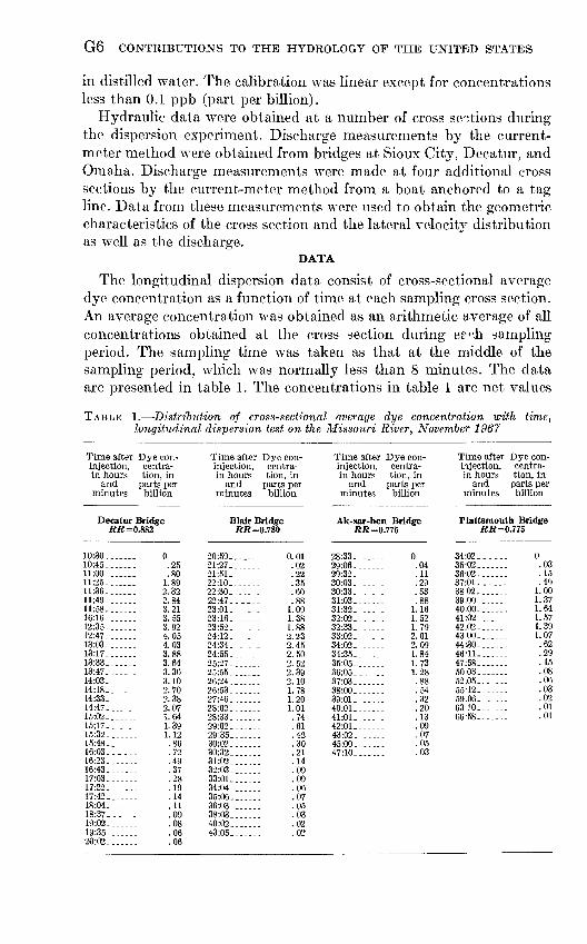
The longitudinal dispersion data consist of cross-sectional average dye concentration as a function of time at each sampling cross section. An average concentration was obtained as an arithmetic average of all concentrations obtained at the cross section during erch sampling period. The sampling time was taken as that at the middle of the sampling period, which was normally less than 8 minutes. The data are presented in table 1. The concentrations in table 1 are net values

TABLE 1. Distribution of cross-sectional average dye concentration with time, longitudinal dispersion test on the Missouri River, November 1967

Time after Dye con- injection, centra- in hours tion, in

and parts per minutes billion

Decatur Bridge RR =0.882

10:30.......10:45... .11:00.......11:25.. .....11:36..... 11:49.. __...11:58.. .....16:16. _._.__12:35-.... .12:47._. .._.13:03_._-___13:17-13:33-_. .__.13:47.14:03.. ___.-14:18-14:33. .._ .14:47-----.-15:02-..-...15:17-. _._._15:32- .-. . 15:48-.__._.16:03-.-..-16:23.......16:43. .17:03- 17:22--- 17:42.... ...18:04.18:37--- -19:02.19:35-_. _.-.20:02.

0 .25 .80

1.89 2.32 2.84 3.21 3.55 3.92 4.05 4.03 3.88 3.64 3.36 3.10 2.70 2.38 2.07 1.64 1.39 1.12 .86 .72 .49 .37 .28 .19 .14 .11 .09 .08 .06 .06

Time after Dye con- injection, centra- in hours tion. in


Blair Bridge RR =0.780

20:59-....._

22:10.......22:30.-... .22:47-....-23:01-___._.

24:12. 24:34- _____ _24:55-_.-__25:27-___._.25:55.____._

26:53__..._.27:46-

29:02.29:35. . .30:02. ,____.30:32. .._..31:02.32:03. .33:01.......34:04-..-.-.35:06-_.._..36:03. . .38:03. .._ .40:0243:05. . . .

0.01 .0299

.35

.60

.88 1.09 1.38 1.88 2.23 2.45 2.50 2.52 2.39 2.10 1.78 1.20 1.01 .74 .61 .42 .30 .21 .14 .09 .09 .06 .07 .05 .03 .02 .02



Ak-sar-ben Bridge RR =0.775

28:33-_. -._.

30:03- _..._.30:33. . . .31:03-.--.31:32. . __32:02-.._._.32:33. - -.33:02-___ 34:02- _.-.._34:35-. _____35:05-. .....36:05. ---_.37:03-, _.__.38:00--.....39:01.......

42:01._ 43:02-_.....45:00. .....47:10.. _____

0 .04 .11.29 .53 .88

1.16 1.52 1.79 2.01 2.09 1.84 1.73 1.28 .88 .54 .32 .20 .13 .09 .07 .05 .03



Plattsmouth Bridge RR= 0.775

34:02----__35-02. 36-02-. ..-. .37:01- --__-38 02. ...._.39.00-. .... .40.00-. ..41:02. 42.02--- 4300- 44:30- ..46-11------47:58--- 5003- 52.05- 55-12----.59.06-----..63?0-___ 66-58- -----

0 .03 .15 .49

1.00 1.37 1.64 1.57 1.39 1.07 .62 .29 .15 .08 .06 .03 .02 .01 .01


(background subtracted) and have not been compensated for dye loss that occurred in the stream. The data are also presented graphically in figure 2. Corresponding data from the 1966 test are included in figure 2 for comparison. Two striking features are evident in this comparison: the differences in the time displacements of the curves and the areas under them. Since the description of these aspects is not the major topic of this report, it is sufficient to say that the shortened travel time in the present test was caused by the reduction of bottom resistance due to a shift from dune-bed to plane-bed. The 1966 test was done under the condition of a dune bed. The difference in the areas under the curves indicates the difference in the observed dye recoveries and is attributed to the difference in the adsorption characteristics between WT dye (present test) and BA dye (1966 test).

10 15 20 25 30 35 40

TIME, IN HOURS AFTER INJECTION

EXPLANATION

50

Cross-sectional average concentration versus time curve resulting from the injection of 120 Ib.of rhodamine WT dye (600 Ib. of 20-percent solution) at Sioux City at 1700 hr., Nov. 13, 1967. Dis charge of 33,300 cfs at Omaha, Nov. 13, 1967.

Cross-sectional average concentration versus time curve resulting from the injection of 125 Ib. rhoda mine BA dye (313 Ib. of 40-percent solution) in jected at Sioux City at 1000 hr., Oct. 4, 1966. Discharge of 31,600 cfs at Omaha, Oct. 3, 1966.

FIGURE 2. Longitudinal dispersion on the Missouri River comparison of the November 1967 data with the October 1966 data.


Values of the recovery ratio, RR, for the present test ar3 also shown in table 1. It is the latio of the amount of dye actually recovered at the cross section to the amount that was injected initially and is computed by a formula

«TJoGdt

where C is the cross-sectional average concentration observed at time t, Q is the discharge, and C0 and V0 are respectively the con centration and the volume of the injected solution. It wrs concluded from the high percentage of recovery that the effect of dye loss on the analysis of dispersion characteristics is negligible in the present test.

The hydraulic data are presented in table 2. The average depth, d, was computed by dividing the area, A, by the surfac^ width, W, while the shear velocity, U*, was computed as the square root of the product gds, where g is the acceleration of gravity and s i^ the energy slope which was assumed to be a constant, 0.0002, for the entire reach.

TABLE 2. Hydraulic data, longitudinal dispersion test on the Missouri River,November 1967

Date Location of cross section Novem

ber

Combination Bridge, Sioux City.__.

Near the mouth of the Little Sioux

1,000 ft upstream from Blair High-

River mile 645, 17,500 ft downstream

Near Plattsmouth Highway Bridge.

131513

14

14

15131615

Cross- Average Average Dis- Channel sectional velocity Average slear

charge width area A YT (fovt depth d velocityQ (cfs) W (feet)

33, 50034, 10031, 200

33,70033, 30033,50034, 000

750755610

600

740577577585

(sq ft) per sec)

8,2208,7807,650

6 OQO

5,8706,3406,3405,634

4.083.88A fift

5.10

5.745.255.286.04

(feet) U*

11.011.612.5

10.7

10.0

7.911.011.09.6

(ft per sec)

0.27.28

OQ

.26

.25

.23

.27

.27

.25

COMPUTATION OF THE LONGITUDINAL DISPERSION COEFFICIENT

ROUTING PROCEDURE

Although several other methods for computing the longitudinal dispersion coefficient are available, the routing procedure presented by Fischer (1968) appears to be the least sensitive to either human judgment or data scatter and produces a coefficient which matches the data as closely as possible. Fischer (1967b) has divided dispersion


into two time periods according to a dimensionless system in which dimensionless time, t' ', is given by

«'=! (2)

In equation 2, t is a time measured from the instant of injection, and T is a time scale given by the relation

I2

in which I is a characteristic length (distance between the maximum velocity thread and the more distant bank) and Ez is the transverse mixing coefficient. As shown in a later section, the measured value of the transverse mixing coefficient for the study reach of the Missouri River is approximately EZ =O.Q U*d. Fischer (1967b) states that if t f , the dimensionless mean time of passage of the tracer cloud past the measuring station, is less than 6, the cloud is in the "convective period," in which the dispersion theory is not applicable. If possible, the routing procedure should be applied using data obtained at measuring stations sufficiently far downstream that the dimensionless mean time of passage past each station is greater than 6.

Table 3 shows the distance downstream from injection, mear time of passage of the tracer cloud, and dimensionless mean time of passage for each of the measurement stations of the present experiment. The reach from Blair to Plattsmouth is entirely within the "difusive period" (£'i>6) and is sufficiently long to permit an accurate calcu lation of the dispersion coefficient. The reach beginning at Decatur is partly within the "convective period," so it yields a somewhat erroneous coefficient; the remainder of the reaches are probably too short to permit accurate calculations.

Table 4 shows the result of applying the routing procedure ir turn from each measured section to each subsequent measured section.

TABLE 3. Time-of-travel data, longitudinal dispersion test on the Missouri River, November 1967

[? is calculated on the basis of the average values Z=450 ft, d=9.68 ft, Z7*=0.250 ft per sec, and T=167 min]

Measurement station

Blair.OmahaPlattsmouth.................

Distance from injection

x, in feet

216,000441 00061? 000796.000

Mean time _of passage t, in minutes

800

2,0802.520

Dimensionless mean time of

passage ?'

4.80.5

12.515.0


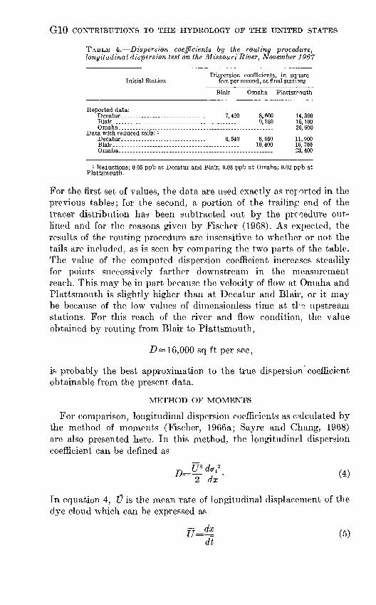
TABLE 4. Dispersion coefficients by the routing procedure, longitudinal dispersion test on the Missouri River, November 1967

Dispersion coefficients, in sq'iare Initial Station feet per second, at final stations

Blair Omaha Plattsrrouth

Reported data:

Data with reduced tails: l

Blair_, __________________________

..._. 7,420 8,600-- -.......... 9,160

----- 6,540 8,660_---___-_-__.____ 10,400

14,30016,10026, 600

11,90016, 70023,400

1 Reductions; 0.05 ppb at Decatur and Blair; 0.03 ppb at Omaha; 0.02 ppb at Plattsmouth.

For the first set of values, the data are used exactly as rep orted in the previous tables; for the second, a portion of the trailing end of the tracer distribution has been subtracted out by the procedure out lined and for the reasons given by Fischer (1968). As expected, the results of the routing procedure are insensitive to whether or not the tails are included, as is seen by comparing the two parts of the table. The value of the computed dispersion coefficient increases steadily for points successively farther downstream in the measurement reach. This may be in part because the velocity of flow at Omaha and Plattsmouth is slightly higher than at Decatur and Blair, or it may be because of the low values of dimensionless time at tH upstream stations. For this reach of the river and flow condition, the value obtained by routing from Blair to Plattsmouth,

Z> = 16,000 sq ft per sec,

is probably the best approximation to the true dispersion coefficient obtainable from the present data.

METHOD OF MOMENTS

For comparison, longitudinal dispersion coefficients as calculated by the method of moments (Fischer, 1966a; Sayre and Chang, 1968) are also presented here. In this method, the longitudinal dispersion coefficient can be defined as

»- In equation 4, U is the mean rate of longitudinal displacement of the dye cloud which can be expressed as

U=^ (5) dt

MIXING CHARACTERISTICS OF THE MISSOURI RIVER Gil

where tis the mean time of passage of the dye cloud from the injection station to a point at distance x downstream from the injection station,

f^tCdt7- Jo - (6)

7T

JoCdt

Another term in equation 4, o-/, is the variance of the concentration versus time curve at x,

/»0

t2Cdt [~t] 2. (7)« .Cdt

Jo

The main difficulty in evaluating D by the method of moments is the large contribution to the variance by the tails of the concentration distributions. Even a small amount of tracer that is temporarily trapped in slow-moving flow near the banks and subsequently released to the main channel, where it shows up as a tail on the concentration distribution, can greatly inflate the value oi D. In anticipation of this problem the curves were truncated at times when concentrations on the recession limbs of the curves reached 3 percent and 1 percent of the peak concentration. The truncations were performed before calculating 7 and a ts by equations 6 and 7. The results are shown in figure 3 and table 5. If the variances corresponding to the 1- and 3- percent truncation levels are considered as maximum and minimum estimates respectively, a reasonable estimate of an average value of D for the entire reach is 15,000 sq ft per sec as shown in figure 3. The values of Z> given in table 5, although somewhat larger than the values for the corresponding subreaches given in table 4, exhibit the same general trend and variation within the reach. On the whole, the values of D calculated by the method of moments compare reasonably well with those determined by the routing procedure, evidently because the channel of the Missouri River in the study reach is sufficiently well maintained that there are few dead zones near the banks crpable of significantly affecting the longitudinal dispersion process.

TRANSVERSE MIXING

DESCRIPTION OF THE TEST REACH

The transverse mixing test was performed in a reach immediately downstream from Blair Highway Bridge, about 85 miles downstream from Sioux City and 56 miles upstream from Plattsmouth. It was


40

30

20

10

I I T

Mean time of passage

1 I

(J=-«!*-=3.64mph

= 5.34fps

12

10

cc

I 6

I I I T

Variance

x Truncation at 1 percent of peak

° Truncation at 3 percent of peak

T

=-^- dfff = 1.93 sq mi per hr

= 15,000 sq ft per sec

I I I I I20 40 60 80 100 120 140

x, IN MILES

FIGURE 3. Measured mean time of passage and variance as functions of distance.


TABLE 5. Dispersion coefficients by the method of moments, longitudinal dispersion test on the Missouri River, November 1967

Dispersion coefficients, in square feet per second, at final stations

Truncation at 1 percent of peak concen tration:

Truncation at 3 percent of peak concen tration:

Blair.. .................................

Blair Omaha

16, 300 16, 300........... 16,300

9, 730 11, 200........... 13,500

Platts- mouth

20,60024, 00033, 600

14, 80018, 30024, 900

selected for the test because of fairly gentle meandering for a 33,000- foot long stretch, availability of a bridge for installing the injection equipment, and not much river traffic. Channel geometry and hy draulic characteristics are as described in the section on the longi tudinal dispersion test. Looking downstream from Blair Highway Bridge, the river meanders gently to the left for about 3.5 miles with the thalweg running near the right bank (see fig. 4), after which the direction of the meander reverses, and the thalweg crosses to the left side. The channel width ranges from 500 to 700 feet, and the average depth is about 9 feet. The variation in water depth and mean velocity across the channel is illustrated in figure 5; one cross section is at 1,000 feet upstream from Blair Highway Bridge, and another is at River Mile 645 or 17,500 feet downstream from the same bridge.

TEST PROCEDURE

A mixture consisting of 150 pounds of 40-percent rhodamine BA solution, 20 gallons of tapwater, and 10 gallons of methyl cellusolve was prepared in a 50-gallon mariotte vessel installed at Blair Highway Bridge on the morning of November 17, 1967. The vessel, a con^tant- head tank designed for maintaining a uniform rate of discharge, was set 200 feet from the pier on the west bank, so that the river discharge was about equally divided on either side. A 50-foot-long garden hose was used to carry the mixture, coming out of a 0.1065- inch orifice, down to a level about 5 feet above the water surface. The mixture dripped freely from the end of the hose into the water. The injection started at 1040 hours and continued until 1420 hours emptying most of the 48-gallon mixture in the vessel. The overall


CHICAGO AND NORTHWESTERN

4

U.S 30

Injection site on I \ Blair Highway Bridge

EXPLANATION

Cross section for dye sampling

Cross section for velocity measurement

River rrrleage643

0 :/4 Vi 34 1 MILE I___i I___i___i

FIGURE 4. Reach of the Missouri River for the transverse mixing test.

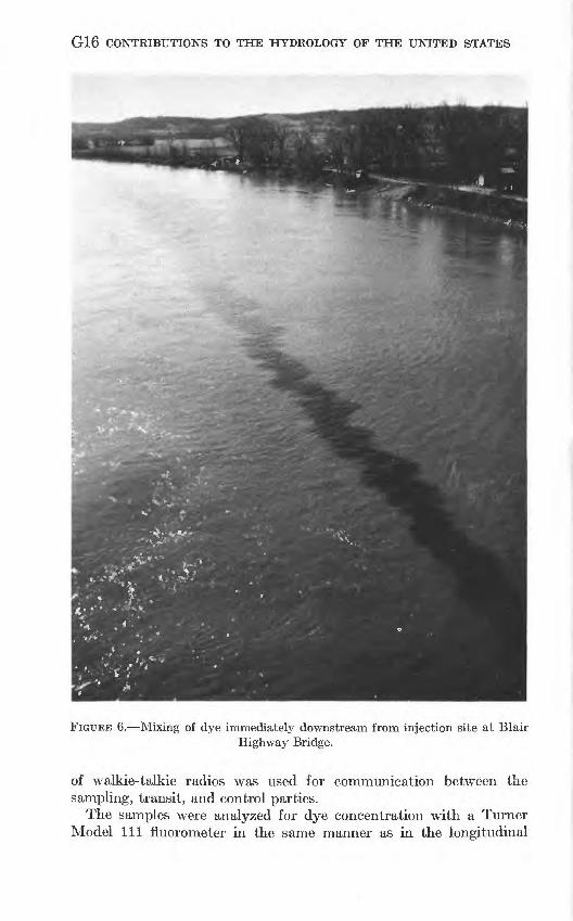
rate of injection was 13.05 ml per sec, and the dye concentration in the mixture was 1.51X108 ppb or 15.1 percent. The pattern of mixing immediately downstream from the injection site is shown in figure 6. The boat ramp on the right bank is about 1,200 feet downstream from the injection site.

Samples for determining the transverse distribution of dye concen tration were collected at 10 cross sections at distances between 1,700 and 33,000 feet downstream from the injection site. The sampling started at the 1,700-foot cross section at 1100 hours and continued until 1509 hours when the sampling at the 33,000-foot cross section


was completed. At each cross section, a sampling boat traversed the channel in a zigzag path along the cross-sectional line marked by three range poles as shown in figure 7. Samples were collected by dipping glass bottles into the water at reasonably uniform intervals so that a minimum of 20 samples was obtained during each traverse. Referring again to the sketch in figure 7, since the length of the base line AB and the angle /3 had been measured previously, the transverse sampling positions could be determined by reading the angle a with a transit at the instant each sample was obtained. A sample was taken immediately upon receiving a signal given by a control party at B when the sampler was in line with the three range poles. Since two transits were available, considerable time was saved by having an advance party set up a transit at the next section downstream. A set

I i1000 feet upstream from Blair Bridge

100 200 300 400 500 600 DISTANCE FROM LEFT BANK, IN FEET

700

FIGURE 5. Observed transverse profiles of velocity and depth at cross sections not affected by bridge abutments.


FIGURE 6. Mixing of dye immediately downstream from injection site at BlairHighway Bridge.

of walkie-talkie radios was used for communication between the sampling, transit, and control parties.

The samples were analyzed for dye concentration with a Turner Model 111 fluorometer in the same manner as in the longitudinal


pole

FIGURE 7. Method for locating lateral sampling positions.

dispersion experiment. Neither the calibration nor the sample read ings were as satisfactory for the BA dye as for the WT dye used in the longitudinal dispersion test. Because of absorption of BA dye on the walls of sampling bottles and perhaps also because of chemical reac tions between the BA dye and impurities in the river water, the cali bration shifted with time. The resulting calibration error was probably on the order of ± 5 percent. The calibration errors together with the sampling scheme, which allowed only one traverse at each cross section, probably caused many of the observed instataneous point concentrations to differ from the time-averaged point concentrations by considerably more than 5 percent.

Velocity measurements by current meter were obtained prior to the test at two cross sections, one 1,000 feet up stream from Blair Highway Bridge on November 14 and the other 17,500 feet down stream from the same bridge on November 15 (see fig. 5). Several available staff gages were read before and after the test to determine the water-surface slope for this reach.


DATA

The transverse mixing data presented in table 6 cons'st of dye concentrations and lateral sampling positions at each cro^s section. Each concentration determined from the surface sampling is assumed to be uniform over the depth and also to be representative, at the particular location, of the time-averaged concentration resulting from the continuous uniform-rate injection of the solute. Values of the recovery ratio, RR, are also shown for each cross section. It is computed by the formula

(*

Q\Jo

cdzRR=

where W is the width of the cross section, and c0 and q$ are respectively the concentration and volumetric discharge rate of the injected dye solution.

TABLE 6.- -Distribution of dye concentration in transverse direction, transverse mixing test on the Missouri River, November 17, 1967

Distance Dye con- from left centra-

Station bank, in tion, in feet parts per

billion



billion

Distance Dye con front left centra-


billion

Cross section 1 X=l,692 ft JF=665ft

123456789

649.1635.6628.5621.2609.5587.9568.2569.6544.3

0.00.13.00.05.00.11.13.03.00

101112131415161718

528.7498.1478.1452.8420.6397.8365.4336.4315.5

.00

.00

.00

.00

.7951.811.41.2.08

1920212223242526

286.4263.8208.9168.6146.7109.468.430.3

.03

.00

.00

.00

.02

.00

.00

.00

Cross section 2 X==3,692 ft IF=735 ft

12345678

706.6687.3682.9668.4647.8622.4608.4587.1

0.00.00.00.02.00.00.00.00

910111213141516

580.7562.2552.7547.1533.6493.7470.4452.2

.00

.001.55.15

4.39.49.65.8

17182022232425

449.5409.4355.1288.1235.1157.579.3

3.092.67.13.00.00.00.00

Cross section 3 X=5,730 ft W=689 ft

RR=0.5S>

123456789

655.9645.1642.1609.9593.0577.4561.6536.1512.3

0.03.00.00.00.00.00.00.00.00

1011121314151617

498.8480.7445.0409.8400.7388.3373.2343.1

.00

.816.376.567.006.125.102.70

1819202122232425

325.8290.9268.1237.3207.2161.9109.944.9

1.41.37

1.20.44.00.00.00.00


TABLE 6. Distribution of dye concentration in transverse direction, transverse mixing test on the Missouri River, November 17, 1967 Continued



billion



billion



billion

Cross section 4 ^"=8,730 ft W=644 ft

##=0.49

13456789

620.4579.9576.7556.3537.3511.2480.4474.3

0.00.02.00.00.02.02

2.201.10

1011121314151617

438.9418.7418.2411.8392.9379.7356.2335.4

5.255.785.685.594.272.653.053.19

18192021222324

308.2275.3225.1200.6157.3112.391.7

.73

.13

.00

.05

.03

.03

.00

Cross section 5 JT=11,850 ft

##=0.65

123456789

605.4591.9580.8564.7549.1533.2518.9497.6481.5

0.00.00.00.00.09.00.13.44.40

101112131415161718

446.4411.7389.8382.1369.4342.1320.3327.8330.2

1.431.873.983.293.823.584.124.025.10

19202122232425

311.0300.3261.7222. 2178.7136.064.1

4.214.312.801.10.54.23.11

Cross section 6 JT= 15,490 ft TF=733 ft ##=0.56

13456789

731.7702.2669.8663.7637.0610.2586.1559.6

0.05.15.23.15.33.75.69.77

1011121314151617

523.8485.8438.1445.4451.6405.2406.6364.1

2.393.634.274.163.003.343.442.49

181920212223

309.5264.3218.5162.1121.348.2

1.10.37.27.35.25.17

Cross section 7 X= 18,720 ft W=657 ft

##=0.66

12345678

627.0607.2590.6568.2549.3516.0560.1524.2

0.33.23.29.23. 29.87.50.58

910111213141516

494.5471.2449. 0419! 6449.0439.0441.8387.0

.831.222.051.641.892.361.512.76

1718192021222324

334.1283.9258.7226.5191.9146.0105.776.2

3.193.82

1.851.10.38.37.50

Cross section 8 JT=22,410 ft W=657 ft

##=0.64

123456789

583.0570.9566.2545.0534.4522.6500.7490.1475.1

0.43.27.25.28.25.31.34.38.44

101112131415161718

474.7442.2424.6398.4366.5338.5307.8291.4272.3

.50

.54

.91

.722.101.552.242.682.51

19202122232425

225.2195.7188.9146.198.660.235.8

3.102.263.253.20.81.58.44


TABLE 6. Distribution of dye concentration in transverse direction, transverse mixing test on the Missouri River, November 17, 1967 Continued



billion



billion

D ist ance D y e co n- fron- left centra-

Station ban!', in tion, in feet parts per

billion

Cross section 9 JT=27,690 ft W=605 ft

I23456789

586.6576.0561.9555.1540.3529.9514.2496.4483.7

0.27.48.19.27.23.25.23.33.23

101112131415161718

467.8453.1440.0414.3371.4364.8337.3308.3255.6

.31

.31

.34

.62

.93

.941.621.802.47

192021222324252627

222.1189.1190.0171.7168.8141.4112.872.922.7

2.832.392.632.742.352.051.511.08.88

Cross section 10 JT=32,970 ft W=509ft

RR=0.5&

8910111213141516

490.6470.4442.5427.3411.1399.5381.8367.1362.8

0.27.27.31.27

.33

.40

.43

.44

171819202122232425

354.6339.6320.3295.6263.1252.7205.8180.7172.0

.44

.46

.481.121.581.822.012.132.26

26272829303132

172,9163,6135 693 074 160,923 5

2.032.082.132.141.471.641.35

COMPUTATION OF THE TRANSVERSE MIXING COEFFICIENT

METHOD OF MOMENTS

For a flow in an infinitely wide, open channel, flowing at a uniform depth and uniform velocity throughout its width, Sayre and Chang (1968) have shown that the transverse mixing coefficient may be calculated by the relationship

(8)

in which Ez is the transverse mixing coefficient, a-2z is the variance of the transverse distribution of the tracer, x is distance downstream from the point of injection of the tracer, and JJ is the mean flow velocity. In a nonuniform stream, such as the Missouri, equation 8, which is derived assuming an equal convective velocity at every point, is not strictly applicable because of the changing pattern of convective velocity. Nevertheless, equation 8 can be applied to the present data to provide a useful first approximation to the correct mixing coeffi cient, at least so long as the tracer distribution is not significantly affected by the presence of the boundaries.


Figure 8 shows a plot of variance of the tracer cloud at each of the first seven measuring stations versus distance downstream from the injection point. Downstream from station 7 significant quantities of tracer had reached the boundaries. The variances were calculated directly from the transverse concentration distributions, without dis charge weighting. Figure 8 shows a reasonably linear increase of the tracer variance for measuring sections 1 through 5; the slope of the straight line of best fit yields a transverse mixing coefficient EZ =1.5G sq ft per sec. On the basis of mean shear velocity U* = 0.24 ft per sec and a mean depth c?=9.1 ft, this yields a dimensionless transverse mixing coefficient El/U*d=0.71.

COMPUTER SIMULATION METHOD

The mixing coefficient calculated by equation 8 is only an approxi mation; because the transverse mixing experiment was conducted over a meandering reach of a river where the velocity is nonuniform across the width and along the length. A more valid method of calculat ing a mixing coefficient must take into account the pattern of convective velocities. In view of the complex pattern of velocity distribution, however, such calculation is only possible through a step-by-step simulation of convective diffusion process by a numerical method. This leads to a trial-and-error method of evaluating the mixing

14,000

Distribution calculated by computer using E, =0.6 u*d

2000 4000 6000 8000 10,000 12,000 14,000 16,000 18.0CO 20,000

DISTANCE DOWNSTREAM FROM INJECTION, IN FEET

FIGURE 8. Variance of transverse tracer distribution, observed and calculated.


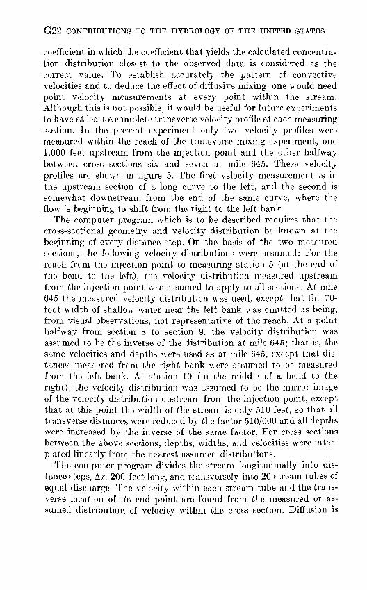
coefficient in which the coefficient that yields the calculated concentra tion distribution closest to the observed data is considered as the correct value. To establish accurately the pattern of convective velocities and to deduce the effect of diffusive mixing, one would need point velocity measurements at every point within the stream. Although this is not possible, it would be useful for future experiments to have at least a complete transverse velocity profile at each measuring station. In the present experiment only two velocity profiles were measured within the reach of the transverse mixing experiment, one 1,000 feet upstream from the injection point and the other halfway between cross sections six and seven at mile 645. The^e velocity profiles are shown in figure 5. The first velocity measurement is in the upstream section of a long curve to the left, and the second is somewhat downstream from the end of the same curve, where the flow is beginning to shift from the right to the left bank.

The computer program which is to be described requires that the cross-sectional geometry and velocity distribution be knowTn at the beginning of every distance step. On the basis of the two measured sections, the following velocity distributions were assumed: For the reach from the injection point to measuring station 5 (at the end of the bend to the left), the velocity distribution measured upstream from the injection point was assumed to apply to all sections. At mile 645 the measured velocity distribution was used, except that the 70- foot width of shallow water near the left bank was omitted as being, from visual observations, not representative of the reach. At a point halfway from section 8 to section 9, the velocity distribution was assumed to be the inverse of the distribution at mile 645; that is, the same velocities and depths were used as at mile 645, except that dis tances measured from the right bank were assumed to b° measured from the left bank. At station 10 (in the middle of a bend to the right), the velocity distribution was assumed to be the mirror image of the velocity distribution upstream from the injection point, except that at this point the width of the stream is only 510 feet, so that all transverse distances were reduced by the factor 510/600 and all depths were increased by the inverse of the same factor. For cross sections between the above sections, depths, widths, and velocities were inter- plated linearly from the nearest assumed distributions.

The computer program divides the stream longitudinally into dis tance steps, Ax, 200 feet long, and transversely into 20 stream tubes of equal discharge. The velocity within each stream tube and the trans verse location of its end point are found from the measured or as sumed distribution of velocity within the cross section. Diffusion is


assumed to be occurring between the stream tubes at a rate given by the Fickian equation

M=Ezas ^ (9)

in which M is the mass transport through the dividing surface between stream tubes per unit time, a s is the dividing area between the stream tubes, and z is the transverse distance. A steady-state equation for the conservation of mass within each stream tube for each distance step is

q.ct+i, i=qct, j+Mj-i, } Mj, j+l (10)

in which q is the discharge per stream tube (constant for all stream tubes), Ct,j is the concentration in the jth stream tube at the start of the -ith distance step, and Mj, j+ i is the rate of mass transfer between streams j' andj + 1. The mass transfer between stream tubes is assumed to be entirely diffusive (that is, any effects of secondary currents are absorbed in the diffusive term), and is calculated by the formula

Mj, J+l=E4u+l*x ^F^1 (11)

in which djtj+ i is the depth at the interface between stream tubes, j andj'+l; and Azjij+i is the distance between the centroids of adjacent stream tubes. The derivation of this formula assumes that for com puting mass transfer the concentration in each of the stream tubes is constant throughout the distance step. The boundary condition of no transport through either bank is satisfied by allowing stream tubes 1 and 20 to exchange only with stream tubes 2 and 19, respectively.

The variation in stream-tube velocity is not shown explicitly in equation 10, but the functional dependence can be seen by substituting equation 11 into equation 10 and dividing the result by g. Dropping the stream-tube subscripts, taking q=uAzd, where u is the local velocity, and, for simplicity, replacing the finite difference form of the transverse concentration gradient by the differential form yield

u 02*

This shows that for a constant mixing coefficient and a constant dis tance step, the change of concentration within a stream tube caused by transverse mixing is inversely proportional to the local velocity, «.

To complete one distance step, the computer carries out the compu tation given in equation 10 for each of the 20 stream tubes lining the


concentration values at the beginning of the distance step, replaces each concentration value by its new value at the end of the distance step, and prints the 20 concentrations. Between distance steps the positions of the midpoints of each of the stream tubes and the depths of the stream tubes may be changed, according to the pattern of convective velocities assumed at the outset. The program is designed to read velocity-distribution data normally recorded in the Geological Survey stream-gaging operations. From these data the coniDuter con structs a set of stream tubes of equal discharge and interpolates stream- tube velocities and dimensions between measuring stations.

Before the program was used in the present experiment, it was verified by assuming a flow having a width of 500 feet, r, depth of 10 feet, a uniform transverse velocity distribution, a mean velocity of 5 ft per sec, and a shear velocity of 0.25 ft per sec. The distance step was taken to be 500 feet and the mixing coefficient 0.23U*d, or (0.575 sq ft per sec). The variance of the tracer cloud produced by the computer program increased exactly linearly with distance, the rate of increase giving a mixing coefficient of 0.56 sq ft per sec by equation 8. The difference between the given mixing coefficient and the computer result is 2.6 percent, well within the level of other experimental errors.

The program was next applied to predict the transverse mixing pattern in the experimental reach by introducing the velocity distri butions previously assumed. The initial tracer distribution was taken to be that measured at measuring section 1, because upstream from section 1 the tracer probably was not fully mixed over the depth. The program then generated tracer distributions at all downstream sections. The computer program is written to accept up to 10 values of k in the mixing coefficient, kU*d, and to generate tracer distribu tions simultaneously for each k value; for this experiment k values of 0.4, 0.5, 0.6, 0.7, and 0.8 were tried. Figure 9 shows the observed tracer distributions and those which were generated by the program using the value fc=0.6. This value produced what appeared to be the best match between observed and computer-predicted concentra tion distributions; much of the error probably results from incorrect assumption of the velocity distribution. However, the comparison is reasonably good at all sections and shows that the equation

#z = 0.6 U*d (12)

gives an adequate prediction of the mixing pattern for the reach in question.

The sensitivity of the mixing pattern to changes in the value of k can be seen in figure 10, which shows the transverse concentration


0 100 200 300 400 500 600 700 TRANSVERSE DISTANCE FROM RIGHT BANK, IN FEET

800

FIGURE 9. Comparison of observed and calculated transverse distribution of dye concentration at nine cross sections


distribution at sections 5 and 9 for k equal to 0.4 and 0.8. The wide range of k produces only a modest change in the distribution; at section 5, 0.4 appears to give the better match, but at section 9, 0.8 appears to be the better choice. Thus the value 0.6 can be regarded only as an adequate approximation, probably accurate to within db 20 percent. Unfortunately there appears to be no more accurate method of measuring the value of the coefficient. The variances of the tracer

10 n i r

EXPLANATION

Observed concentration

Concentration calculated by computer

with £~ = Q.4U*d

CO 7

04

Section 5

with f, =0.8U*d

100 200 300 400 500 TRANSVERSE DISTANCE FROM RIGHT BANK, IN FEET

600

100 200 300 400 500 TRANSVERSE DISTANCE FROM RIGHT BANK, IN FEET

600

FIGURE 10. Influence of E, on transverse distribution of dye concentration.


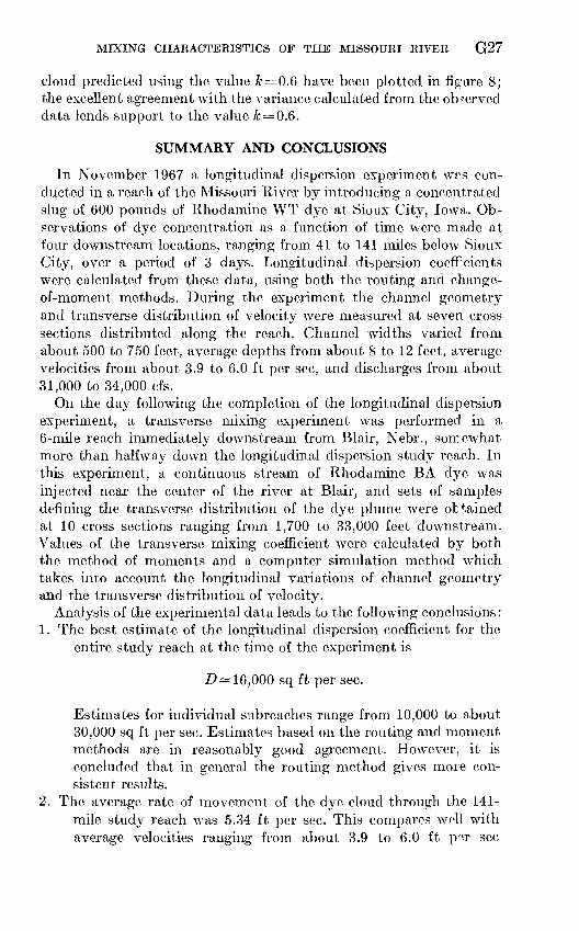
cloud predicted using the value k=O.Q have been plotted in figure 8; the excellent agreement with the variance calculated from the observed data lends support to the value fc = 0.6.

SUMMARY AND CONCLUSIONS

In November 1967 a longitudinal dispersion experiment WPS con ducted in a reach of the Missouri River by introducing a concentrated slug of 600 pounds of Rhodamine WT dye at Sioux City, Iowa. Ob servations of dye concentration as a function of tune were made at four downstream locations, ranging from 41 to 141 miles below Sioux City, over a period of 3 days. Longitudinal dispersion coeffcients were calculated from these data, using both the routing and change- of-moment methods. During the experiment the channel geometry and transverse distribution of velocity were measured at seven cross sections distributed along the reach. Channel widths varied from about 500 to 750 feet, average depths from about 8 to 12 feet, average velocities from about 3.9 to 6.0 ft per sec, and discharges from about 31,000 to 34,000 cfs.

On the day following the completion of the longitudinal dispersion experiment, a transverse mixing experiment was performed in a 6-mile reach immediately downstream from Blair, Nebr., son:ewhat more than halfway down the longitudinal dispersion study reach. In this experiment, a continuous stream of Rhodamine BA dye was injected near the center of the river at Blair, and sets of samples defining the transverse distribution of the dye plume were ottained at 10 cross sections ranging from 1,700 to 33,000 feet downstream. Values of the transverse mixing coefficient were calculated by both the method of moments and a computer simulation method which takes into account the longitudinal variations of channel geometry and the transverse distribution of velocity.

Analysis of the experimental data leads to the following conclusions:1. The best estimate of the longitudinal dispersion coefficient for the

entire study reach at the time of the experiment is

D~ 16,000 sq ft per sec.

Estimates for individual subreaches range from 10,000 to about 30,000 sq ft per sec. Estimates based on the routing and moment methods are in reasonably good agreement. However, it is concluded that in general the routing method gives more con sistent results.

2. The average rate of movement of the dye cloud through the 141- mile study reach was 5.34 ft per sec. This compares well with average velocities ranging from about 3.9 to 6.0 ft p 0,r sec


measured by current meter at various cross sections through the reach.

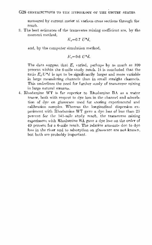
3. The best estimates of the transverse mixing coefficient are, by the moment method,

#2 =0.7 U*d,

and, by the computer simulation method,

#2 =0.6 U*d.

The data suggest that Ez varied, perhaps by as much as 100 percent within the 6-mile study reach. It is concluded that the ratio Ez/U*d is apt to be significantly larger and more variable in large meandering channels than in small straight channels. This underlines the need for further study of transverse mixing in large natural streams.

4. Bhodamine WT is far superior to Rhodamine BA as a water tracer, both with respect to dye loss in the channel and aclsorb- tion of dye on glassware used for storing experimental and calibration samples. Whereas the longitudinal dispersion ex periment with Rhodamine WT gave a dye loss of less than 25 percent for the 141-mile study reach, the transverse mixing experiment with Rhodamine BA gave a dye loss on the order of 40 percent for a 6-mile reach. The relative amounts due to dye loss in the river and to adsorption on glassware are not known, but both are probably important.


REFERENCES

Bowie, J. E., and Petri, L. R., 1968, Travel of solutes in lower Missouri River:U.S. Geol. Survey Hydrol. Inv. Atlas HA-332.

Elder, J. W., 1959, The dispersion of marked fluid in turbulent shear flew: Jour.Fluid Mechanics, v. 5, no. 4, p. 544-560.

Fischer, H. B., 1966a, A note on the one dimensional dispersion model: Airand Water Pollution, an Internat. Jour., v. 10, p. 443-452.

Fischer, H. B., 1966b, Longitudinal dispersion in laboratory and natural streams:California Inst. Tech., W. M. Keck Lab. Hydraulic and Water Resources,Rept. KH-R-12, 250 p.

Fischer, H. B., 1967a, Transverse mixing in a sand-bed channel: U.S. Geol.Survey Prof. Paper 575-D, p. D277-D282.

Fischer, H. B., 1967b, The mechanics of dispersion in natural streams: Jour.Hydraulics Div., Am. Soc. Civil Engineers, v. 93, no. HY6, p. 187-216.

Fischer, H. B., 1968, Dispersion predictions in natural streams: Jour. SanitaryEngineering Div., Am. Soc. Civil Engineers, v. 94, no. SA5, p. 927-943.

Glover, R. E., 1964, Dispersion of dissolved or suspended materials in flowingstreams: U.S. Geol. Survey Prof. Paper 433-B, 32 p.

Godfrey, R. G., and Frederick, B. J., 1963, Dispersion in natural streams: U.S.Geol. Survey open-file report, 75 p.

Sayre, W. W., and Chang, F. M., 1968, A laboratory investigation of open- channel dispersion processes for dissolved, suspended, and floating dis-persants, U.S. Geological Survey Prof. Paper 433-E, 71 p.

Taylor, G. E., 1954, The dispersion of matter in turbulent flow through a pipe:Royal Soc. London Proc., v. 223A, p. 446-468.

Thackston, E. L., and Krenkel, P. A., 1966, Longitudinal mixing and reaerationin natural streams: Vanderbilt Univ. Sanitary and Water Resources Eng.,Tech. Rept. 7,212 p.

Thackston, E. L., and Krenkel, P. A., 1967, Longitudinal mixing in naturalstreams: Jour. Sanitary Engineering Div., Am. Soc. Civil Engineers, v. 93,no. SA5, p. 67-190.

U.S. Army Corps of Engineers, Omaha District, 1967, Missouri River Channelregime studies: M.R.D. (Missouri River Division) Sediment Series 13, 13 p.

Wilson, J. F., and Forrest, W. E., 1965, Potomac River time-of-travel measure ments: Lamont Geol. Observatory Symposium on Diffusion in Oceans andFresh Waters, Palisades, N.Y., 1964, Proc., p. 1-18.

Yotsukura, Nobuhiro, 1967, General discussion in subject D microturbulentdiffusion and dispersion: Internat. Assoc. Hydraulic Research Cone;., 12th,Fort Collins, Colo., 1967, Proc., v. 5, p. 542-551.

US. GOVERNMENT PRINTING OFFICE: 1970 O 37F-385