BRITISH STANDARD BS 1042-1.4:1992Incorporating Amendment No. 1

Measurement of fluid flow in closed conduits —

Part 1: Pressure differential devices —

Section 1.4 Guide to the use of devices specified in Sections 1.1 and 1.2

BS 1042-1.4:1992

This British Standard, having been prepared under the direction of theIndustrial-process Measurement and Control Standards Policy Committee, was published under the authority of the Standards Board and comesinto effect on31 March 1992

© BSI 12-1998

First published March 1984Second edition March 1992

The following BSI references relate to the work on this standard:Committee reference PCL/2 Special announcement in BSI News, September 1991

ISBN 0 580 20404 9

Committees responsible for this British Standard

The preparation of this British Standard was entrusted by theIndustrial-process Measurement and Control Standards Policy Committee (PCL/-) to Technical Committee PCL/2, upon which the following bodies were represented:

British Compressed Air SocietyBritish Gas plcDepartment of Energy (Gas and Oil Measurement Branch)Department of Trade and Industry (National Engineering Laboratory)Electricity Industry in United KingdomEnergy Industries CouncilGAMBICA (BEAMA Ltd.)Institute of Measurement and ControlInstitute of PetroleumInstitute of Trading Standards AdministrationInstitution of Gas EngineersInstitution of Mechanical EngineersSociety of British Gas IndustriesWater Services Association of England and Wales

The following bodies were also represented in the drafting of the standard, through subcommittees and panels:

Engineering Equipment and Materials Users’ AssociationInstitution of Water and Environmental ManagementUnited Kingdom Offshore Operators’ Association

Amendments issued since publication

Amd. No. Date Comments

8154 June 1994 Indicated by a sideline in the margin

BS 1042-1.4:1992

© BSI 12-1998 i

Contents

PageCommittees responsible Inside front coverForeword ii

Section 1. General1 Scope 12 Symbols 1

Section 2. Calculations3 General 24 Information required 25 Basic equations 36 Calculation of orifice or throat diameter 37 Calculation of rate of flow 10

Section 3. Physical data8 Properties 129 Density of fluid 1210 Viscosity of fluid 1411 Isentropic exponent 14

Section 4. Additional information on measurements and on pulsating and swirling flow12 Measurements 1513 Pulsating flow 2014 Swirling flow 23

Appendix A References for physical data 24

Index 25

Figure 1 — Possible locations of density meters 17 Figure 2 — Multiplying factors for thermal expansion 19 Figure 3 — Damping pulsations in gas flow 22 Figure 4 — Damping pulsations in liquid flow 22

Table 1 — Symbols 1Table 2 — Approximate values of CEb2 for square-edged orifice plates with corner, D, D/2 or flange taps as appropriate 5Table 3 — Approximate values of CEb2 for ISA 1932 nozzles, and rough cast, machined and rough welded convergent venturi tubes 6Table 4 — Approximate values of CEb2 for long radius nozzles 7Table 5 — Approximate values of CEb2 for quarter circle orifice plates 8Table 6 — Approximate values of CEb2 for eccentric orifice plates 8Table 7 — Physical properties of selected liquids 12 Table 8 — Physical properties of selected gases 13

BS 1042-1.4:1992

ii © BSI 12-1998

Foreword

This Section of BS 1042 has been prepared under the direction of the Industrial-process Measurement and Control Standards Policy Committee. It supersedes BS 1042-1.4:1984, which is withdrawn.This is Section 1.4 of a series of Sections of BS 1042 on the measurement of fluid flow in closed conduits, as follows:Section 1.1 Specification for square-edged orifice plates, nozzles and venturi tubes in circular cross section conduits running fullSection 1.2 Specification for square-edged orifice plates and nozzles (with drain holes, in pipes below 50 mm diameter, as inlet and outlet devices) and other orifice platesSection 1.3 Method of measurement of gas flow by means of critical flow Venturi nozzles.Section 1.5 Guide to the effect of departure from the conditions specified in Section 1.1Section 1.1 specifies the geometry and method of use of orifice plates, nozzles and Venturi tubes inserted in conduit running full, to measure the flowrate of the fluid in the conduit. It is technically equivalent to ISO 5167:1980 published by the International Organization for Standardization (ISO). It should be noted that guidance on the effects of departure from the conditions specified in BS 1042-1.1 can be found in BS 1042-1.5:1987.An index to Sections 1.1, 1.2 and 1.4 is provided in this Section, to facilitate the rapid cross-referencing of subject matter.A British Standard does not purport to include all the necessary provisions of a contract. Users of British Standards are responsible for their correct application.

Compliance with a British Standard does not of itself confer immunity from legal obligations.

Summary of pagesThis document comprises a front cover, an inside front cover, pages i and ii, pages 1 to 33 and a back cover.This standard has been updated (see copyright date) and may have had amendments incorporated. This will be indicated in the amendment table on the inside front cover.

BS 1042-1.4:1992

© BSI 12-1998 1

Section 1. General

1 ScopeThis Section of BS 1042 provides sample calculations, physical data and other additional information for using the pressure differential devices specified in BS 1042-1.1 and BS 1042-1.2.

NOTE The titles of the publications referred to in this standard are listed on the inside back cover.

2 SymbolsThe symbols used in this standard are given in Table 1.

Table 1 — Symbols

Symbol Represented quantity DimensionsM: massL: lengthT : timeu: temperature

SI unit

A Cross-sectional area L2 m2

C Coefficient of discharge, dimensionless

d Diameter of orifice or throat of primary device at operating conditions

L m

D Upstream internal pipe diameter at operating conditions L mE Velocity of approach factor, dimensionless

FA, FB Correction factors dimensionless

k Uniform equivalent roughness L mp Static pressure of the fluid ML–1T –2 Pa

qm Mass flowrate MT –1 kg/s

qv Volume flowrate L3T –1 m3/sRe Reynolds number dimensionlessReD, Red

Reynolds number referred to D or d dimensionless

t Temperature of the fluid u ºCX

Acoustic ratio, dimensionless

a Flow coefficient dimensionlessb

Diameter ratio, dimensionless

Dp Differential pressure ML –1T–2 Pa

´ Expansibility (expansion) factor dimensionlessk Isentropic exponent dimensionlessm Dynamic viscosity of the fluid ML–1T –1 Pa·s

y Kinematic viscosity of the fluid, L2T –1 m2/s

r Density of the fluid ML–3 kg/m3

t Pressure ratio, dimensionless

NOTE 1 Other symbols used in this standard are defined at their place of use.NOTE 2 Some of the symbols used in this standard are different from those used in BS 1042-1.1.NOTE 3 Subscript 1 refers to the cross section at the plane of the upstream pressure tapping. Subscript 2 refers to the cross section at the plane of the downstream pressure tapping.

C α E------=

E 1 β4–( ) ½ c–

=

X p∆

Pik--------=

β dD-----=

υ µρ---=

τp2

p1------=

BS 1042-1.4:1992

2 © BSI 12-1998

Section 2. Calculations

3 General In clauses 4 to 7, typical design calculations for the design of orifice plates, nozzles, venturi tubes and venturi nozzles are given.The principal design calculations that are commonly required for pressure differential devices are:

a) assessment of the differential pressure and calculation of the diameter of an orifice (or nozzle or venturi throat) for a stated flow of a given fluid in a given pipe at specified conditions of pressure and temperature;b) calculation of the differential pressure for a stated flow of a given fluid at known temperature and pressure, for a pressure differential device and pipe of known diameter;c) calculation of the flowrate, given the fluid, pressure differential device diameter and pipe diameter, differential pressure and fluid pressure and temperature;d) calculation of the overall uncertainty of the installation for a given flowrate.

Items a) and d) are particularly relevant to the design of a new installation whereas b) and c) are applicable to working installations. The method of calculating the overall uncertainty is described in clause 11 of BS 1042-1.1:1992.The precise sequence of the calculation will depend upon the information required and on the choice of pressure differential device.The calculations are based on the assumption that the size of the pipe needed to carry the fluid is known.

4 Information required4.1 General

The following information is required regarding the installation:

a) maximum, normal and minimum flowrates (i.e. will one flowmeter cover this flow range?);NOTE Where reference volumes are used, the pressure and temperature should be clearly stated; general statements such as “standard pressure and temperature (S.T.P.)” should not be relied upon.

b) accuracy required;c) maximum permissible pressure loss.

4.2 Pipe

The following information is required regarding the pipe:

a) material, temperature coefficient of expansion;b) operating temperature;

c) internal diameter, how obtained (the mean of six measurements or as specified in the relevant pipe standards), uniformity;d) layout, e.g. upstream, downstream fittings, straight lengths (influence on b limits);e) attitude, i.e. vertical, horizontal or sloping;f) internal roughness of pipe.

4.3 Pressure differential device

The following information is required regarding the pressure differential device:

a) type (e.g. squared-edged orifice plate, nozzle, venturi);b) suitability for the application;c) limits on d, D, b and ReD;d) mounting, i.e. slip plate, carrier;e) tappings, i.e. location, number of, diameter;f) material, temperature coefficient of expansion, operating temperature;g) diameter;h) drain hole diameter;i) strength of orifice plate material to calculate deformation under flow conditions.

4.4 Fluid

The following information is required regarding the fluid:

a) state and composition;b) operating temperature and pressure (and local barometric pressure if appropriate);c) density at operating conditions;NOTE For gases density at reference conditions is also often required.

d) viscosity at operating conditions;e) for compressible fluids only, isentropic exponent (ratio of specific heats for ideal gases);f) nature of flow, i.e. viscous or turbulent.

4.5 Differential pressure measuring device

The following information is required regarding the differential pressure measuring device:

a) type (microdisplacement, displacement), wet or dry (i.e. manometric or mechanical), calibration correction factors;b) span (fixed or adjustable), maximum permitted pressure loss for the installation in question;c) maximum operating pressure and temperature of the pressure difference measuring device;d) corrosion resistance (to metered fluid).

BS 1042-1.4:1992

© BSI 12-1998 3

4.6 Basic equations

The basic equations for the following are required:a) mass flow or volumetric flow;b) compressible or incompressible fluids;c) Reynolds number;d) uncertainties.

5 Basic equationsIn the calculation sequences that follow, SI units are used. If it is the user’s practice to use other units, these should be converted into the appropriate SI units.The following equations for mass flowrate, qm, and volume flowrate, qv, are given in 5.1 ofBS 1042-1.1:1992.

where:

If the flowmeter is to be calibrated in units of volume flowrate referred to standard (or other specified) conditions of pressure and temperature, qo, then the following equation should be used, the suffix “0” denoting standard conditions of pressure and temperature.

The above equations enable calculations described in items a) to c) of clause 3 to be made. Since a, C, E, d and p are unknown, the equations can be transposed to:

The values of d and D in the above equations are to be corrected for the effect of fluid temperature. At temperatures within 10 °C of the temperature at which D and d are determined, the measured diameter values are sufficiently accurate, but at temperatures outside this range, corrections for expansion or contraction are necessary.It is also convenient to transpose the equations for Reynolds number (ReD and Red) given in 3.3.2 of BS 1042-1.1:1992 into the following.

and

NOTE In the equations for mass flowrate the dynamic viscosity, m, is used and for volume flowrate the kinematic viscosity, y, is used. However, as the dynamic viscosity is equal to the kinematic viscosity multiplied by the density, the appropriate viscosity can be obtained.

6 Calculation of orifice or throat diameter6.1 General

The procedure for assessment of the differential pressure and calculation of the orifice or throat diameter to measure a stated flowrate of a given fluid in a given pipeline at specified conditions of pressure and temperature is described. The relevant clause references are given at the beginning of each step.

6.2 ProcedureNOTE See clauses 6 and 7 of BS 1042-1.1:1992, sections 2 and 3 of BS 1042-1.2:1989 and 4.2 and 4.3 of this standard).

Before proceeding with the details of the calculation, check the suitability of the device for the application in question and the general acceptability of the pipeline configuration.NOTE The example for each item is given in the corresponding item of 6.3.

a) Calculate the pipe internal diameter, D, at the operating temperature, t °C, preferably using the measured diameter or if this is not possible the diameter obtained from the relevant pipe standards. (See 12.2.)b) Obtain/calculate the fluid density at reference conditions (required only for gas flows measured in volume units at reference conditions of pressure and temperature). Obtain the compressibility factor of the gas at operating conditions.

qm αε π4--- d2 2∆pρ1( )

12⁄=

CEε π4--- d2 2∆pρ1( )

12⁄=

qv αε π4--- d2 2∆p ρ1⁄( )

12⁄=

CEε π4--- d

2 2∆ p ρ1⁄( )1

2⁄=

E 1 1 β4–( )1

2⁄⁄=

β d D⁄=

qo qvρ 1

ρ 0-------=

CEβ2 4qm

επD2

2∆pρ1( )1

2⁄-----------------------------------------------=

4qv

επD2 2∆ p ρ1⁄( )12⁄

-----------------------------------------------------=

ReD4qm

πDµ1----------------

4qv

πDυ1----------------= =

Red4qm

πdµ1---------------

4qv

πdµ1---------------= =

BS 1042-1.4:1992

4 © BSI 12-1998

c) Obtain/calculate the density and the kinematic or dynamic viscosity of the fluid at operating conditions.d) Select appropriate equations from clause 5 for CEb2 and ReD according to whether the flowrate is given for mass or volume.e) Choose a value of D p taking account of the required pressure loss. Check that (pl – Dp)/pl is not less than 0.75. If it is, choose a smaller value of Dp. (It is desirable to keep (pl – Dp)/pl as close to unity as possible.)f) Calculate CEb2 appropriate to the device to be used (orifice plate, nozzle, venturi). If the value obtained is outside the range specified for the particular device, the lower (or upper) limits on b and d for the device will not be met. Choose another value of Dp and repeat e) and f). When continuous flow measurements are required over a range of flows, the ReD value used in these calculations should be calculated using 70 % of the maximum flow to be encountered. (See clause 4, 6.2.2.2, 6.2.3.2, 6.3.2.2, 6.3.3.2, 7.2, 8.2 and 9.2 and of BS 1042-1.2:1989 and Table 2 to Table 6 of this standard.) g) When an acceptable value of CEb2 has been obtained, calculate the approximate values of b and d. The calculation procedure is dependent on the device to be used, as follows.

1) Square-edged orifice plates, D $ 50 mm, use Table 22) ISA 1932 nozzles and rough cast, machined and rough welded convergent venturi tubes, use Table 3.3) Long radius nozzles use Table 4.4) Square-edged orifice plates in the size range 25 # D < 50 mm;NOTE The Stolz equation for corner tappings given in 8.3.2.1 of BS 1042-1.1:1992 is used for deriving the discharge coefficients provided the minimum Reynolds numbers are above the following values.

Re $ 40 000b2 for 0.23 # b # 0.5Re $ 10 000 for 0.5 # b # 0.7

5) Square-edged orifice plates with corner tappings when measuring flow into a large space, use procedures 1) and 4).6) ISA 1932 nozzles and venturi nozzles when measuring flow into a large space, use procedure 2).7) Quarter circle orifice plates, use Table 5.8) Eccentric orifice plates, use Table 6.9) Conical entrance orifice plates, calculate b directly. (See 7.5.1 of BS 1042-1.2:1989.)

10) Square-edged orifice plates with corner tappings when measuring flow from a large space, calculate b directly. (See 6.2.2.3 of BS 1042-1.2:1989.) 11) ISA 1932 nozzles and venturi nozzles when measuring flow from a large space, calculate b directly. (See 6.2.3.3 of BS 1042-1.2:1989.)

NOTE b can be calculated directly for procedures 9) to 11) because C has a single predetermined value.

h) Check that the Reynolds number, ReD or Red, is within the permitted limits for the device. If the Reynolds number is greater than the upper limit, then D or d is too small. If the Reynolds number is less than the lower limit, try increasing Dp by reducing d and go back to e).i) Calculate the relative roughness criterion appropriate to the pipeline material and diameter and check that it is within the permitted limits for the device used. This is vital for high accuracy measurements, especially if D is small. (See 8.3.1, 9.1.6.2, 9.2.6.1 and 10.1.2.6 of BS 1042-1.1:1992.) j) Calculate the expansibility factor (´ = 1 for liquids). There is one equation for square-edged orifices, and another for nozzles and venturis. Use b obtained in g). Note that the acoustic ratio X in the orifice plate equation is equal to Dp/p1k, where k is the isentropic exponent.For nozzles and venturis, the pressure ratio, t, which is equal to 1 – Dp/pl is also required. When continuous flow measurements over a range of flows is required and ReD is based on 70 % of the maximum flow [see step f)] then 50 % of the Dp value chosen in step e) should be used. (See 8.3.2.2, 9.1.6.3, and 10.1.6 ofBS 1042-1.1:1992 and 6.2.2.4, 6.2.3.4, 7.5.2, 8.5.2 and 9.4.3 of BS 1042-1.2:1989.)k) Calculate a revised value of CEb2 by dividing the value obtained in f) by ´. Update the value of b as in step g).l) Use the revised value of b to calculate C (or a) from the appropriate equation. Use C, and the revised value of b to calculate CEb2 (note that E = 1(1 – b4)½). Compare this result with that of step k). Adjust the value of b and repeat this step until there is agreement to within 0.05 %. (See 8.3.2.1, 9.1.6.2, 9.2.6.2, 10.1.5.2 and 10.1.5.4 of BS 1042-1.1:1992 and 6.2.2.3, 6.2.3.3, 7.5.1, 8.5.1 and 9.4.1 of BS 1042-1.2:1989.)m) Calculate d from b and D corrected for operating temperature.

BS 1042-1.4:1992

© BSI 12-1998 5

n) Correct the value of d obtained in m) to ambient temperature. This is the diameter to which the orifice or throat will be machined unless drain holes are required.

o) Correct d to allow for a drain hole, if appropriate. (See clause 4 of BS 1042-1.2:1989.)

Table 2 — Approximate values of square of CEb2 for square-edged orifice plates with corner, D, D/2 or flange taps as appropriate

b CEb2 for a Reynolds number, ReD, of:

5 × 103 104 2 × 104 3 × 104 5 × 104 7 × 104 105 106 107 108

0.23 0.0318 0.0317 0.0317 0.0316 0.0316 0.0316 0.0316 0.0316 0.0316 0.0316

0.24 0.0347 0.0346 0.0345 0.0345 0.0344 0.0344 0.0344 0.0344 0.0344 0.0344

0.26 0.0409 0.0407 0.0406 0.0405 0.0405 0.0405 0.0405 0.0404 0.0404 0.0404

0.28 0.0475 0.0473 0.0472 0.0471 0.0471 0.0470 0.0470 0.0470 0.0469 0.0469

0.30 0.0548 0.0544 0.0543 0.0542 0.0541 0.0541 0.0541 0.0540 0.0540 0.0540

0.32 0.0626 0.0621 0.0619 0.0618 0.0617 0.0617 0.0617 0.0616 0.0616 0.0616

0.34 0.0709 0.0704 0.0701 0.0700 0.0699 0.0698 0.0698 0.0697 0.0697 0.0697

0.36 0.0799 0.0792 0.0789 0.0787 0.0786 0.0785 0.0785 0.0783 0.0783 0.0783

0.38 0.0895 0.0887 0.0882 0.0880 0.0879 0.0878 0.0877 0.0875 0.0875 0.0875

0.40 0.0998 0.0987 0.0982 0.0979 0.0977 0.0976 0.0975 0.0973 0.0973 0.0973

0.42 0.1108 0.1095 0.1087 0.1085 0.1082 0.1081 0.1080 0.1077 0.1076 0.1076

0.44 0.1225 0.1209 0.1200 0.1196 0.1193 0.1192 0.1191 0.1187 0.1186 0.1186

0.46 0.1350 0.1330 0.1319 0.1315 0.1311 0.1310 0.1308 0.1304 0.1303 0.1303

0.48 — 0.1459 0.1446 0.1441 0.1437 0.1435 0.1432 0.1427 0.1426 0.1426

0.50 — 0.1595 0.1580 0.1574 0.1569 0.1566 0.1564 0.1558 0.1556 0.1556

0.52 — 0.1741 0.1723 0.1716 0.1709 0.1706 0.1704 0.1696 0.1694 0.1694

0.54 — 0.1896 0.1874 0.1867 0.1858 0.1855 0.1852 0.1842 0.1840 0.1840

0.56 — 0.2061 0.2035 0.2026 0.2017 0.2012 0.2009 0.1997 0.1995 0.1995

0.58 — 0.2238 0.2207 0.2197 0.2185 0.2180 0.2177 0.2162 0.2159 0.2159

0.60 — 0.2427 0.2389 0.2376 0.2364 0.2358 0.2353 0.2336 0.2333 0.2333

0.62 — 0.2628 0.2584 0.2568 0.2555 0.2547 0.2541 0.2522 0.2518 0.2517

0.64 — 0.2842 0.2793 0.2774 0.2758 0.2749 0.2743 0.2719 0.2714 0.2714

0.66 — 0.3072 0.3016 0.2994 0.2975 0.2965 0.2957 0.2929 0.2923 0.2923

0.68 — 0.3319 0.3256 0.3229 0.3208 0.3195 0.3187 0.3153 0.3146 0.3145

0.70 — 0.3584 0.3499 0.3482 0.3458 0.3443 0.3433 0.3393 0.3385 0.3383

0.72 — 0.3871 0.3772 0.3757 0.3729 0.3711 0.3699 0.3646 0.3635 0.3634

0.74 — 0.4183 0.4068 0.4056 0.4025 0.4003 0.3988 0.3925 0.3912 0.3910

0.76 — 0.4522 0.4390 0.4378 0.4345 0.4325 0.4305 0.4231 0.4216 0.4213

0.78 — — 0.4756 0.4734 0.4702 0.4682 0.4658 0.4567 0.4549 0.4547

0.80 — — 0.5129 0.5117 0.5081 0.5061 0.5052 0.4941 0.4919 0.4916

BS 1042-1.4:1992

6 © BSI 12-1998

Table 3 — Approximate values of CEb2 for ISA 1932 nozzles, and rough cast, machined and rough welded convergent venturi tubes

b CEb2 for venturi tubes CEb2 for ISA 1932 nozzles for a Reynolds number, ReD, of:

Machined Rough cast

Rough welded

2 × 104 3 × 104 5 × 104 7 × 104 105 106 107

0.30 — — — — 0.0887 0.0890 0.0891 0.0892 0.0893 0.0893

0.316 — 0.0889 — —

0.32 — 0.1013 — — 0.1009 0.1013 0.1014 0.1015 0.1017 0.1017

0.34 — 0.1145 — — 0.1139 0.1143 0.1145 0.1147 0.1149 0.1149

0.36 — 0.1286 — — 0.1277 0.1283 0.1285 0.1286 0.1289 0.1289

0.38 — 0.1436 — — 0.1423 0.1430 0.1433 0.1435 0.1438 0.1438

0.40 0.1613 0.1595 0.1597 — 0.1578 0.1587 0.1589 0.1591 0.1596 0.1596

0.42 0.1783 0.1763 0.1765 — 0.1741 0.1751 0.1754 0.1757 0.1762 0.1763

0.44 0.1963 0.1942 0.1944 0.1898 0.1913 0.1924 0.1929 0.1932 0.1938 0.1938

0.46 0.2154 0.2130 0.2133 0.2007 0.2094 0.2107 0.2112 0.2116 0.2123 0.2123

0.48 0.2356 0.2330 0.2332 0.2265 0.2285 0.2299 0.2305 0.2309 0.2317 0.2318

0.50 0.2569 0.2541 0.2543 0.2464 0.2485 0.2502 0.2508 0.2513 0.2521 0.2522

0.52 0.2795 0.2764 0.2766 0.2673 0.2697 0.2715 0.2722 0.2727 0.2736 0.2737

0.54 0.3033 0.3000 0.3003 0.2893 0.2919 0.2939 0.2946 0.2952 0.2962 0.2963

0.56 0.3286 0.3250 0.3253 0.3125 0.3153 0.3174 0.3183 0.3188 0.3199 0.3200

0.58 0.3554 0.3515 0.3519 0.3372 0.3401 0.3422 0.3431 0.3438 0.3449 0.3450

0.60 0.3839 0.3797 0.3801 0.3631 0.3662 0.3684 0.3693 0.3700 0.3712 0.3713

0.62 0.4143 0.4097 0.4101 0.3908 0.3938 0.3961 0.3970 0.3977 0.3989 0.3990

0.64 0.4467 0.4418 0.4423 0.4202 0.4232 0.4254 0.4263 0.4269 0.4281 0.4282

0.66 0.4815 0.4762 0.4767 0.4617 0.4544 0.4565 0.4574 0.4580 0.4591 0.4592

0.68 0.5189 0.5132 0.5137 0.4853 0.4878 0.4897 0.4904 0.4910 0.4919 0.4920

0.70 0.5598 0.5531 0.5537 0.5216 0.5236 0.5251 0.5257 0.5262 0.5270 0.5270

0.72 0.6032 0.5965 — 0.5610 0.5623 0.5633 0.5637 0.5640 0.5645 0.5645

0.74 0.6512 0.6440 — 0.6041 0.6044 0.6046 0.6046 0.6047 0.6048 0.6048

0.76 — — — 0.6514 0.6504 0.6495 0.6492 0.6490 0.6486 0.6485

0.78 — — — 0.7040 0.7012 0.6990 0.6982 0.6975 0.6964 0.6963

0.80 — — — 0.7632 0.7579 0.7540 0.7525 0.7513 0.7493 0.7491

BS 1042-1.4:1992

© BSI 12-1998 7

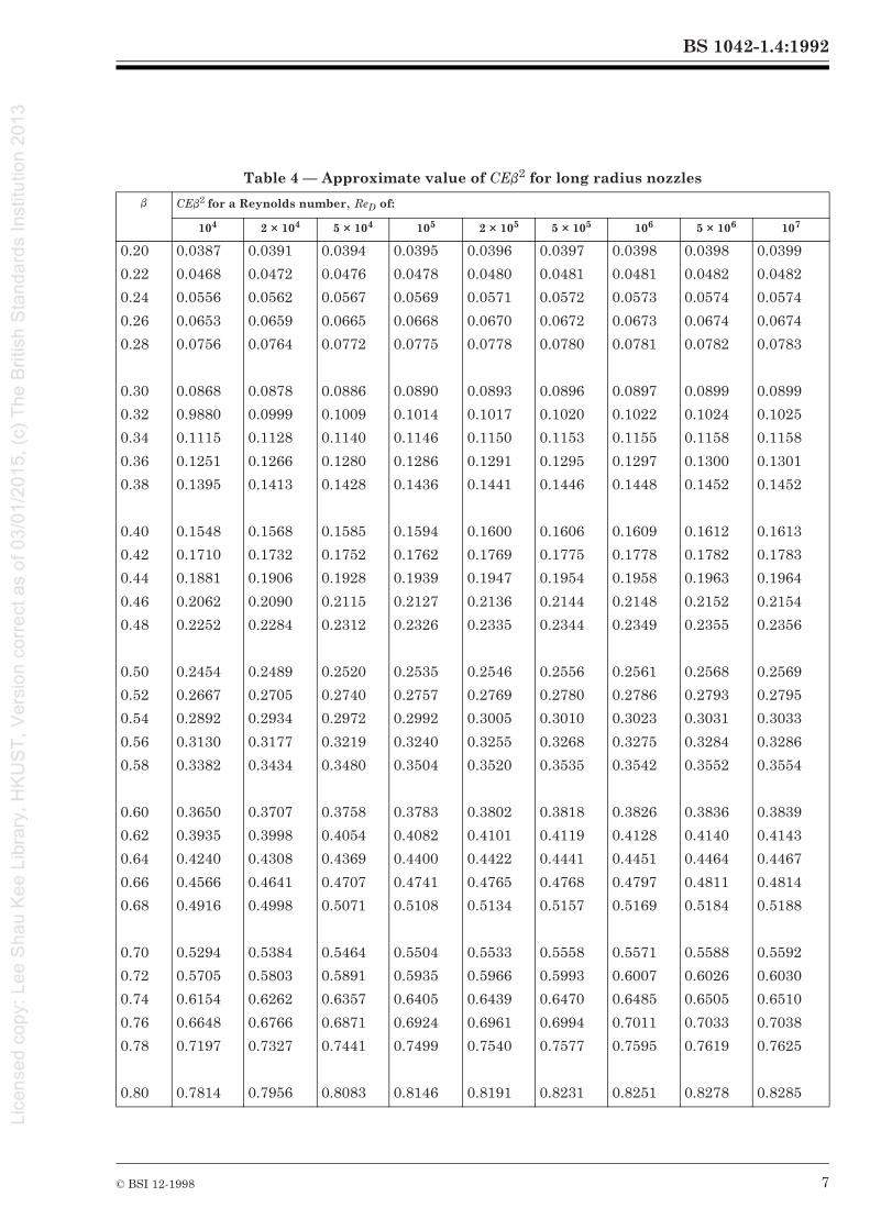
Table 4 — Approximate value of CEb2 for long radius nozzles

b CEb2 for a Reynolds number, ReD of:

104 2 × 104 5 × 104 105 2 × 105 5 × 105 106 5 × 106 107

0.20 0.0387 0.0391 0.0394 0.0395 0.0396 0.0397 0.0398 0.0398 0.0399

0.22 0.0468 0.0472 0.0476 0.0478 0.0480 0.0481 0.0481 0.0482 0.0482

0.24 0.0556 0.0562 0.0567 0.0569 0.0571 0.0572 0.0573 0.0574 0.0574

0.26 0.0653 0.0659 0.0665 0.0668 0.0670 0.0672 0.0673 0.0674 0.0674

0.28 0.0756 0.0764 0.0772 0.0775 0.0778 0.0780 0.0781 0.0782 0.0783

0.30 0.0868 0.0878 0.0886 0.0890 0.0893 0.0896 0.0897 0.0899 0.0899

0.32 0.9880 0.0999 0.1009 0.1014 0.1017 0.1020 0.1022 0.1024 0.1025

0.34 0.1115 0.1128 0.1140 0.1146 0.1150 0.1153 0.1155 0.1158 0.1158

0.36 0.1251 0.1266 0.1280 0.1286 0.1291 0.1295 0.1297 0.1300 0.1301

0.38 0.1395 0.1413 0.1428 0.1436 0.1441 0.1446 0.1448 0.1452 0.1452

0.40 0.1548 0.1568 0.1585 0.1594 0.1600 0.1606 0.1609 0.1612 0.1613

0.42 0.1710 0.1732 0.1752 0.1762 0.1769 0.1775 0.1778 0.1782 0.1783

0.44 0.1881 0.1906 0.1928 0.1939 0.1947 0.1954 0.1958 0.1963 0.1964

0.46 0.2062 0.2090 0.2115 0.2127 0.2136 0.2144 0.2148 0.2152 0.2154

0.48 0.2252 0.2284 0.2312 0.2326 0.2335 0.2344 0.2349 0.2355 0.2356

0.50 0.2454 0.2489 0.2520 0.2535 0.2546 0.2556 0.2561 0.2568 0.2569

0.52 0.2667 0.2705 0.2740 0.2757 0.2769 0.2780 0.2786 0.2793 0.2795

0.54 0.2892 0.2934 0.2972 0.2992 0.3005 0.3010 0.3023 0.3031 0.3033

0.56 0.3130 0.3177 0.3219 0.3240 0.3255 0.3268 0.3275 0.3284 0.3286

0.58 0.3382 0.3434 0.3480 0.3504 0.3520 0.3535 0.3542 0.3552 0.3554

0.60 0.3650 0.3707 0.3758 0.3783 0.3802 0.3818 0.3826 0.3836 0.3839

0.62 0.3935 0.3998 0.4054 0.4082 0.4101 0.4119 0.4128 0.4140 0.4143

0.64 0.4240 0.4308 0.4369 0.4400 0.4422 0.4441 0.4451 0.4464 0.4467

0.66 0.4566 0.4641 0.4707 0.4741 0.4765 0.4768 0.4797 0.4811 0.4814

0.68 0.4916 0.4998 0.5071 0.5108 0.5134 0.5157 0.5169 0.5184 0.5188

0.70 0.5294 0.5384 0.5464 0.5504 0.5533 0.5558 0.5571 0.5588 0.5592

0.72 0.5705 0.5803 0.5891 0.5935 0.5966 0.5993 0.6007 0.6026 0.6030

0.74 0.6154 0.6262 0.6357 0.6405 0.6439 0.6470 0.6485 0.6505 0.6510

0.76 0.6648 0.6766 0.6871 0.6924 0.6961 0.6994 0.7011 0.7033 0.7038

0.78 0.7197 0.7327 0.7441 0.7499 0.7540 0.7577 0.7595 0.7619 0.7625

0.80 0.7814 0.7956 0.8083 0.8146 0.8191 0.8231 0.8251 0.8278 0.8285

BS 1042-1.4:1992

8 © BSI 12-1998

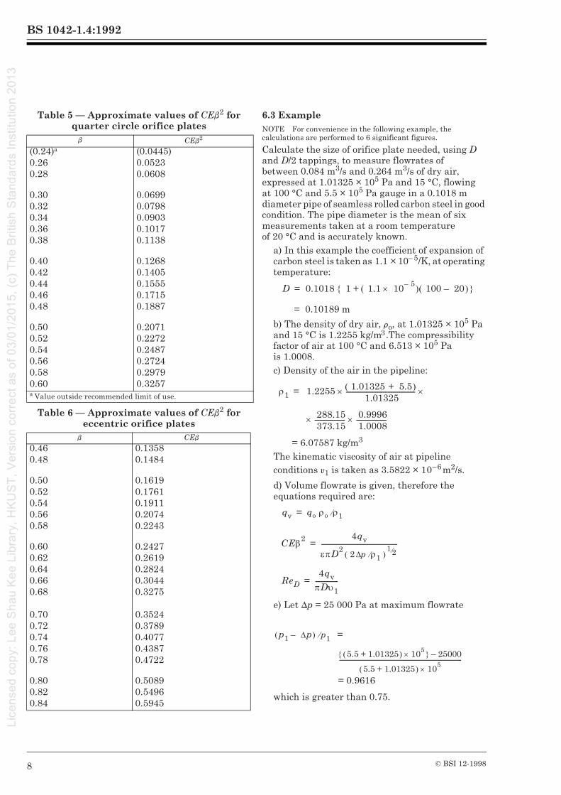
Table 5 — Approximate values of CEb2 for quarter circle orifice plates

Table 6 — Approximate values of CEb2 for eccentric orifice plates

6.3 ExampleNOTE For convenience in the following example, the calculations are performed to 6 significant figures.

Calculate the size of orifice plate needed, using D and D/2 tappings, to measure flowrates of between 0.084 m3/s and 0.264 m3/s of dry air, expressed at 1.01325 × 105 Pa and 15 °C, flowing at 100 °C and 5.5 × 105 Pa gauge in a 0.1018 m diameter pipe of seamless rolled carbon steel in good condition. The pipe diameter is the mean of six measurements taken at a room temperature of 20 °C and is accurately known.

a) In this example the coefficient of expansion of carbon steel is taken as 1.1 × 10– 5/K, at operating temperature:

b) The density of dry air, ro, at 1.01325 × 105 Pa and 15 °C is 1.2255 kg/m3 .The compressibility factor of air at 100 °C and 6.513 × 105 Pa is 1.0008. c) Density of the air in the pipeline:

= 6.07587 kg/m3

The kinematic viscosity of air at pipeline conditions y1 is taken as 3.5822 × 10–6m2/s.

d) Volume flowrate is given, therefore the equations required are:

e) Let Dp = 25 000 Pa at maximum flowrate

which is greater than 0.75.

b CEb2

(0.24)a (0.0445)0.26 0.05230.28 0.0608

0.30 0.06990.32 0.07980.34 0.09030.36 0.10170.38 0.1138

0.40 0.12680.42 0.14050.44 0.15550.46 0.17150.48 0.1887

0.50 0.20710.52 0.22720.54 0.24870.56 0.27240.58 0.29790.60 0.3257a Value outside recommended limit of use.

b CEb

0.46 0.13580.48 0.1484

0.50 0.16190.52 0.17610.54 0.19110.56 0.20740.58 0.2243

0.60 0.24270.62 0.26190.64 0.28240.66 0.30440.68 0.3275

0.70 0.35240.72 0.37890.74 0.40770.76 0.43870.78 0.4722

0.80 0.50890.82 0.54960.84 0.5945

=

= 0.9616

D 0.1018 1 1.1 10 5–×( ) 100 20–( )+{ }=

0.10189 m=

ρ1 1.2255 1.01325 5.5+( ) 1.01325

-------------------------------------------- ××=

288.15 373.15--------------------× 0.9996

1.0008--------------------×

qv qo ρo ρ1⁄=

CEβ2 4qv

επD22 ∆p ρ1⁄( )

1 2⁄------------------------------------------------------=

ReD4qv

πDυ1----------------=

p1 ∆p–( ) p1⁄

5.5 1.01325+( ) 105×{ } 25000–

5.5 1.01325+( ) 105×---------------------------------------------------------------------------------------

BS 1042-1.4:1992

© BSI 12-1998 9

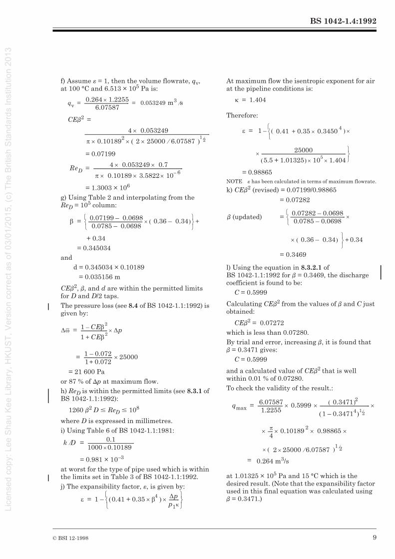
f) Assume ´ = 1, then the volume flowrate, qv, at 100 °C and 6.513 × 105 Pa is:

CEb2 =

= 0.07199

= 1.3003 × 106

g) Using Table 2 and interpolating from the ReD = 105 column:

+ 0.34= 0.345034

andd = 0.345034 × 0.10189

= 0.035156 m

CEb2, b, and d are within the permitted limits for D and D/2 taps.The pressure loss (see 8.4 of BS 1042-1.1:1992) is given by:

= 21 600 Paor 87 % of Dp at maximum flow.h) ReD is within the permitted limits (see 8.3.1 of BS 1042-1.1:1992):

1260 b2 D # ReD # 108

where D is expressed in millimetres.i) Using Table 6 of BS 1042-1.1:1981:

= 0.981 × 10–3

at worst for the type of pipe used which is within the limits set in Table 3 of BS 1042-1.1:1992.j) The expansibility factor, ´, is given by:

At maximum flow the isentropic exponent for air at the pipeline conditions is:

Therefore:

= 0.98865NOTE ´ has been calculated in terms of maximum flowrate.

k) CEb2 (revised) = 0.07199/0.98865

l) Using the equation in 8.3.2.1 ofBS 1042-1.1:1992 for b = 0.3469, the discharge coefficient is found to be:

C = 0.5999

Calculating CEb2 from the values of b and C just obtained:

CEb2 = 0.07272which is less than 0.07280.By trial and error, increasing b, it is found that b = 0.3471 gives:

C = 0.5999

and a calculated value of CEb2 that is well within 0.01 % of 0.07280.To check the validity of the result.:

at 1.01325 × 105 Pa and 15 °C which is the desired result. (Note that the expansibility factor used in this final equation was calculated using b = 0.3471.)

qv 0.264 1.2255×

6.07587--------------------------------------------- 0.053249 m3 s⁄= =

4 0.053249×

π 0.101892 2 25000 6.07587⁄×( )1

2⁄××------------------------------------------------------------------------------------------------------------------------------

ReD 4 0.053249× 0.7×

π 0.10189× 3.5822× 10 6–×---------------------------------------------------------------------------------=

β 0.07199 0.0698– 0.0785 0.0698–------------------------------------------------- 0.36 0.34–( )×

+=

∆ω 1 CEβ2–

1 CEβ2+

--------------------------- ∆p×=

1 0.072–1 + 0.072-------------------------- 25000×=

k D⁄ 0.11000 0.10189×-----------------------------------------------=

ε 1 0.41 0.35 β4×+( ) ∆pp1κ---------×

–=

= 0.07282

b (updated) =

= 0.3469

= 0.264 m3/s

κ 1.404=

ε 1 0.41 0.35+ 0.3450 4×( ) ×

–=

25000

5.5 1.01325+( ) 105× 1.404×

-------------------------------------------------------------------------------------×

0.07282 0.0698– 0.0785 0.0698–

------------------------------------------------------- ×

0.36 0.34–( ) ×

0.34+

qmax 6.07587 1.2255

------------------------- 0.5999× 0.3471( ) 2

1 0.34714–( )12⁄

--------------------------------------------------× ×=

π 4-----× 0.10189 2× 0.98865× ×

2 25000 6.07587⁄×( ) 1 2⁄×

BS 1042-1.4:1992

10 © BSI 12-1998

m) There is no drain hole, and at pipeline temperature:

d = 0.10189 × 0.3471= 0.03537 m

n) Correct d for room temperature:

d = 0.03537 {1 + (1.8 × 10–5)(100 – 20)}= 35.32 mm

NOTE For this correction, the coefficient of expansion of stainless steel, from which the plate will be made, is taken as 1.8 × 10–5/K.

7 Calculation of rate of flow7.1 General

The procedure for calculation of the flowrate, given the pipe and orifice diameters, the physical properties of the flowing fluid, the type of primary device used and the measured pressure difference is described.NOTE The example for each item is given in the corresponding item of 7.3.

7.2 ProcedureNOTE See 4.2 and 4.3.

Before proceeding with the details of the calculation, check that the pipeline configuration is acceptable.

a) Calculate the pipe internal diameter, D, and the orifice (or throat) diameter, d, at the operating temperature t °C. (See 12.2.)b) Calculate the diameter ratio, b.c) Check that D, d and b are within the limits specified in this standard for the device in question.d) Obtain the density, r1 and dynamic viscosity m1 of the flowing fluid at pipeline conditions. If they are not quoted explicitly in the calculation information summary:

1) use relevant tables of physical data;2) (see section 3) calculate r1 and m1 from values found in tables at reference conditions; and3) if the flowrate is required in units of volume (per unit time) at reference conditions of pressure and temperature, the density r0 at these conditions is also required.

e) Select appropriate equations from clause 5 for the flowrate and Reynolds number, ReD, according to whether mass or volume flowrate is required.f) Assume a value of 106 for the Reynolds number.g) Calculate an interim value for the discharge coefficient, C (or the flow coefficient if appropriate). (See 6.2 k) and 6.2 l).)

h) Check that (p1 – Dpmax)/p1 is not less than 0.75.i) Check that the roughness of the pipe is within limits. (See 6.2 i).)j) Calculate the expansibility factor (a = 1 for liquids). Note that the isentropic exponent or the ratio of specific heats is required. (See 6.2 j).)k) Use the above data and the interim value of C to calculate an approximate value of the flowrate.l) Calculate the Reynolds number, ReD.m) Calculate a precise value of C using the above value of ReD.n) Calculate a revised value of the flowrate.o) Repeat the procedure from l) to n) until the difference between the last two calculations of flowrate is less than one part in 106.

7.3 ExampleNOTE For convenience in the following example, the calculations are performed to 6 significant figures.

Steam at 20 × 105 Pa absolute and 250 °C is flowing in a well-lagged pipeline. A square-edged orifice plate with corner taps is installed at a distance equal to 50 times the pipe diameter downstream of a single right-angle bend. Another bend is situated at a distance equal to at least 20 times the pipe diameter downstream of the orifice plate. The measured diameters of the pipe (carbon steel) and orifice (stainless steel) are 0.152 m and 0.0835 m respectively. The measured pressure difference is 2.5 × 104 Pa.Calculate the mass flowrate in kg/s.Reference to 7.2 and Table 1 of BS 1042-1.1:1992 shows that the pipeline configuration is acceptable, even without calculating the diameter ratio.

a) At pipeline temperature:

b) b = d/D= 0.55O223

c) Referring to 8.3.1 of BS 1042-1.1:1992:b is within limits: 0.23 # b # 0.8d is within limit: d $ 12.5 mm.D is within limits: 50 mm # D # 1 000 mm

d) The density of steam at 20 × 105 Pa and 250 °C is 8.9686 kg/m3.

D = 0.152 {1 + (1.1 × 10–5) ×× = (250 – 20)} = 0.152385 m

d = 0.0835 {1 + (1.8 × 10–5) ×× (250 – 20)}

= 0.0838457 m

BS 1042-1.4:1992

© BSI 12-1998 11

The dynamic viscosity at 20 × 105 Pa and 250 °C is 1.82 × 10–5 Pa·s.e) The mass flowrate is required, therefore the equations to be used are:

f) ReD = 106 (assumed). g) From 8.3.2.1 of BS 1042-1.1:1992:

h) = 0.9875which is greater than 0.75. i) It is assumed for the purposes of this example that the relative roughness of the pipe walls, k/D is less than 3.8 × 10– 4 (see 8.3.1 ofBS 1042-1.1:1992).j) For steam, the isentropic exponent, k, is 1.31.

where

k) The approximate flowrate is given by:

l) The Reynolds number:

m) The value of C:

n) The revised value of the flowrate:qm = 2.33282 kg/s

o) The revised Reynolds number:

ReD = 1070970

p) The revised value of C:C = 0.603871

q) The newly revised (and final) value of the flowrate:

qm = 2.33282 kg/s

C = 0.5959 + 0.0312bb2.1 – 0.184bb8 +

= 0.603903

´ = 1 – (0.41 + 0.35b4)X

= 1 – (0.41 + 0.35 × 0.5502234)X

X =

=

´ = 0.995782

qm CEε π4--- d2 2∆p r1( )

12⁄=

ReD4qm

πDµ1----------------=

0.0029β 2.5 106

ReD-----------

0.75

+

p 1 ∆p–( ) p 1 2000000 25000–( ) 2000000⁄=

∆pp1k----------

25000 2000000 1.31×--------------------------------------------

qm =

=

× 0.995782 ×

× 8.9686)½

= 2.33295 kg/s

ReD=

= 1071030

C =

= 0.603871

CEε π 4----- d 2 2∆pρ 1( )

1 2⁄

0.603903 1

1 0.550223 4–

---------------------------------------------- 1

2⁄ ××

π 4-----× 0.0838457( )

2× 2 25000× ×(×

4 2.33295×

π 0.152385× 1.82× 10 5–×

---------------------------------------------------------------------------------------

0.5959 0.0312β 2.1 0.184β8 +–+

0.0029β 2.5 10 6

1071030---------------------------

0.75

+

BS 1042-1.4:1992

12 © BSI 12-1998

Section 3. Physical data

8 PropertiesIn clauses 9 to 11, information is given to assist the user in determining the physical fluid properties needed for the calculation of the flowrate and the Reynolds number. The properties dealt with are density and viscosity of fluids and the isentropic exponents of gases.

9 Density of fluid 9.1 General

The density of the fluid at the upstream tapping can be determined using a density meter or by measurements of the fluid pressure, temperature and composition. For direct measurement of density using a density meter, see 12.1.

9.2 Density of liquids

The density of liquids varies with temperature; the variation with pressure is so slight that it may usually be ignored. The densities of several liquids at standard reference conditions are given inTable 7 and recommended sources of data for the physical properties of liquids are listed in Appendix A.

9.3 Density of mixtures of liquids

The density (in kg/m3) of a mixture of liquids can often be approximated assuming that the volumes of the components are additive:

where:

where:

The error involved in assuming that the volumes of the components are additive is in general less the more closely the liquids are related chemically. The assumption is not as a rule valid for mixtures of concentrated solutions of electrolytes.

9.4 Density of gases

The density of gases varies with the temperature and pressure and, for moist gases, with the amount of water vapour present. The densities of several dry gases at standard reference conditions are given in Table 8 and recommended sources of data for the physical properties of gases are listed in Appendix A. Gas density variation with temperature and pressure is given by the gas laws, deviations from the laws for perfect gases being allowed for by a compressibility factor (see 9.8).For dry gases, density can be obtained from the following equation:

The density of moist gases at pressures close to atmospheric pressure can be calculated from the following equation:

where:

Table 7 — Physical properties of selected liquids

r1, r2 are the densities of the component liquids (in kg/m3) at the working conditions;

v1, v2 are the percentages by volume of the components.

r = 100/(m1/r1 + m2/r2+...)

m1, m2 are the percentages by mass of the components.

ρ ρ1υ1 ρ2υ2 ....+ +( ) 100⁄=p is the absolute pressure of the fluid at the

upstream tapping (in Pa);

t is the temperature of the fluid at the upstream tapping (in °C);

pv is the partial pressure of the water vapour at the upstream tapping (in Pa);

Zg and Zv are the compressibility factors for the dry gas and the water vapour present respectively (dimensionless);

Rg and Rv are the gas constants for the gas and water vapour respectively [in J/(kg·K)].

ρ pZgRg t 273.15+( )----------------------------------------------=

ρp pv–

ZgRg t 273.15+( )----------------------------------------------

pv

ZvRv t 273.15+( )----------------------------------------------+=

Liquid Density at reference conditions

Dynamic viscosity at reference conditions

Melting point Boiling point

kg/m3 mPa·s K K

Carbon tetrachloride 1 584 969 250 349.8Ethyl alcohol 789.4 1 189 159 351.4Glycerine 1 261 1 410 × 103 291.0 563.0Kerosines 740 to 840 1 000 to 2 000 below 240 420 to 570Water 998.2 1 002 273.15 373.15NOTE Reference conditions: 20 °C, 101.325 kPa

BS 1042-1.4:1992

© BSI 12-1998 13

Table 8 — Physical properties of selected gases

9.5 Density of gas mixtures

When a gas mixture is to be metered and conditions are such that the constituent gases can be considered to be ideal the density of the mixture can be calculated from the following equation:

where:RM is the gas constant for the mixture given by the following equation:

where:R1 and R2 are the gas constants for gases 1 and 2 respectively;m1 and m2 are the percentages by mass of the components.

When the gases cannot be considered to be ideal, methods such as those given in the reference of Appendix A should be used.

9.6 Density of fluid containing impurities

When the fluid contains impurities (in small amounts), the effective density may differ from that of the pure fluid. When the effective density is that of the combined system of pure fluid plus impurities, it is given by either of the following equations:

where:

9.7 Partial pressure of water vapour

The partial pressure of water vapour, pv (in Pa) is required for calculating the density of moist gases. Determination of the value to two significant figures is adequate. The partial pressure can be found from hygrometric measurements or calculated from the amount of water vapour present by means of one of the following equations.

a) If the absolute humidity, Hv, (that is the mass of water vapour present in unit volume of moist gas expressed in kg/m3) is known then:

where:t is the temperature at the upstream tapping (in °C).

Gas Relative molecular

mass

Density at reference conditions

Dynamic viscosity at reference conditions

Isentropic exponent at

reference conditions

Critical temperature

Critical pressure

Gas constant

kg/m3 mPa·s K MPa J/(kg·K)

Air 28.96 1.2255 17.96 1.4021 132.55a 3.769a 287.1

Ammonia 17.03 0.7298 10.4 1.32 405.6 11.28 488.2

Carbon dioxide 44.01 1.8922 14.40 1.3000 304.0 7.38 188.9

Carbon monoxide 28.01 1.1860 17.23 1.399 132.91 3.499 296.8

Ethylene 28.054 1.1783 9.99 1.250 282.55 5.05 296.4

Hydrogen 2.02 0.08527 8.730 1.406 33.20 1.297 4116.0

Methane 16.04 0.6804 10.80 1.31 190.53 4.595 518.4

Nitrogen 28.01 1.1861 17.32 1.401 126.2 3.39 296.8

Oxygen 32.00 1.3553 20.15 1.397 154.58 5.043 259.8

Propane 44.10 1.92 7.87 1.14 369.82 4.249 188.5

Steam 18.02 — — — 647.14 22.05 461.4a Indicates gas mixture where composition can change around the critical region.

NOTE Reference conditions: 15 °C, 101.325 kPa

ρ pRM t 273.15+( )---------------------------------------------=

RM1

100----------- m1R1 m2R2 ...+ +( )=

ρ ρf υi ρi( ρf ) 100⁄–+=

rf is the density of the pure fluid (in kg/m3);

ri is the density of the impurities (solid, liquid or gas) (in kg/m3);

vi is the percentage by volume of gaseous impurities;

mi is the percentage by mass of solid or liquid impurities.

ρ ρf 1 mi ρf ρi–( ) 100ρi⁄+( )⁄=

pv 464.9Hv t 273.15+( )=

BS 1042-1.4:1992

14 © BSI 12-1998

b) If the moisture content, Hw, (that is the mass of water vapour present in unit mass of dry gas, both masses being expressed in the same units) is known then:

where:

c) If the relative humidity, w, (that is, the ratio of the actual vapour pressure, pv, to the saturation vapour pressure at the same temperature) is known then:

where:pvs is the saturation vapour pressure at the temperature at the upstream tapping.

Accurate measurement of the amount of water vapour present (the absolute humidity, Hv, or the moisture content, Hw,) is difficult, particularly in the presence of solid impurities and condensible vapours. The best method is often to take a representative sample of the moist gas from a tapping point upstream of the device (but close to it), care being taken to avoid premature condensation, and then to determine by chemical absorption the weight of water vapour contained in the sampled volume.At temperatures below 150 °C the relative humidity, w, of moist air can be found by means of wet and dry bulb thermometers exposed to a stream of air sampled from the upstream pipeline.NOTE For further information, reference should be made to BS 1339.

9.8 Compressibility factor

The ideal gas equation modified for use with real gases may be given as:

where:

For a perfect gas obeying the ideal laws, Z is constant and equal to unity for all temperatures and pressures. For real gases the compressibility factor, Z, serves as a measure of the extent of the departure from the ideal gas and this allows the density of the gas to be calculated. Values of Z for various gases may be found in the references listed in Appendix A.

10 Viscosity of fluid10.1 General

The dynamic viscosity (commonly called the absolute viscosity) of the fluid at the upstream pressure tapping is required for calculating the Reynolds number. It is sufficiently precise if the viscosity is known to two significant figures.

10.2 Viscosity of liquids

While the viscosity of liquids is influenced by both temperature and pressure, in most cases it varies with temperature but barely at all with pressure. The dynamic viscosities of various selected liquids at standard reference conditions are given inTable 7 and further information on viscosities may be found from the references listed in Appendix A. Methods for measuring the viscosity of liquids are described in BS 188.

10.3 Viscosity of gases and vapours

The viscosities of gases and vapours vary with temperature and pressure. The dynamic viscosities of selected gases at standard reference conditions are listed in Table 8 and further information on the viscosities of gases may be found from the references listed in Appendix A, where references for the viscosity of steam are also given.

11 Isentropic exponentThe isentropic exponent, k, which is needed to calculate the expansibility factor decreases with increase of temperature and increases with increase in pressure. At atmospheric pressure and room temperature the value is about 1.4 for diatomic gases such as O2, H2, CO, Cl2, and air and about 1.3 for triatomic gases such as CO2 and steam. Values of the isentropic exponent for several gases are listed in Table 8 and further information may be obtained from the references listed in Appendix A.

p is the absolute pressure at the upstream tapping (in Pa);

Mw and Mg are the relative molecular masses of the water vapour and gas respectively.

Z is the compressibility factor;

r is the mass density of the fluid;

R is the gas constant;

t is the temperature of the fluid (in °C).

pvHwp

Mw

Mg----------

Hw+

-------------------------------=

pv ϕpvs=

p ZρR t 273.15+( )=

BS 1042-1.4:1992

© BSI 12-1998 15

Section 4. Additional information on measurements and on pulsating and swirling flow12 Measurements12.1 Direct density measurement

12.1.1 General

In 5.4.3 of BS 1042-1.1:1992, it is stated that the mass density of the fluid can be measured directly provided that the method employed does not disturb the flow measurement. While fluid density at the pressure differential device upstream tapping is frequently determined from fluid pressure and temperature measurements it is also often desirable to employ direct density measurements.Commercially available density meters are based on several different physical principles and are made in many varieties. Some of the more common principles are:

a) vibration, where the frequency of vibration of an immersed element depends upon the fluid density;b) Archimedes, where the buoyancy of an immersed object depends upon the fluid density;c) neucleonic, where the absorption of radiation depends upon the density of the absorbing medium;d) Clausius-Mosotti, where the dielectric strength of a fluid is related to its density;e) acoustic, where the speed of sound through the fluid is related to its density;f) centrifugal, where the pressure rise due to centrifugal forces depends upon the fluid density.

For use in quantity measuring of flow the density meter should be suitable for continuous on-line measurement.

12.1.2 Density meter installationNOTE Because of the wide variety of density meters available, it is not possible to give details of all of the types of installation.

It is most important to ensure that the fluid in the density meter is at the same pressure and temperature as the fluid it is desired to measure, or sufficiently close to keep errors within acceptable limits.The flowrate through the density meter should be optimized to give a reasonable response time to changes in density and maintain the desired temperature. Too high a flowrate can cause problems due to pressure losses and turbulent noise.

The flow direction through the density meter should be chosen to encourage self-cleaning. With gases, vertically downward flow will help prevent the build-up of any solid particles or liquid drops.With liquids, vertically upward flow will help prevent the build-up of any gas bubbles. Care should be taken to avoid phase changes in the density meter, particularly condensation with gases and flashing with liquids due to temperature and pressure changes.It is important that temperature differences (between flowmeter and density meter) and temperature gradients (between instruments and their surroundings) be avoided by the use of thermal insulation where necessary.All density meter installations should be designed to facilitate maintenance and calibration checks.Differences in installation allow density meters to be divided into two distinct types as follows:

a) Direct insertion density meters. The direct insertion of the density meter in the pipeline ensures that the fluid in the density meter is at the same pressure and temperature as that in the pipeline. The pipeline should be large enough to accommodate the meter with acceptably low pressure loss.b) Bypass sampling system. For a bypass sampling system a suitable pressure differential device or pump is required to drive the sample flow around the system. Ensuring a representative sample at the correct pressure and temperature can prove difficult and the density meter should preferably be in physical contact with the pipeline for example by mounting it in thermal contact with the pipe. Both the density meter and associated pipework should be thermally lagged to achieve an acceptable temperature equilibrium.

If filters are used in the system, their pressure loss should be considered.

BS 1042-1.4:1992

16 © BSI 12-1998

12.1.3 Density meter locations

At first sight it would appear that there is more freedom in the location of a density meter in liquid service than in gas. With incompressible liquids the density is not affected by local pressure changes in the vicinity of the flowmeter, hence, provided there are not marked temperature changes, all densities are the same. With a compressible gas the density changes with pressure and temperature and can be measured only where the corresponding expansibility factor, ´, is known. However other limits of temperature and pressure capacity and sufficient flow are so severe that the differences between gas and liquid service become minor and they can be considered together. Four examples of possible density meter locations are shown in Figure 1, and further details are as follows.

a) Upstream of flowmeter. A direct insertion density meter can be placed sufficiently far upstream of the flowmeter not to interfere with it or upstream of a flow straightener that eliminates flow disturbances produced by the meter. For this type of installation care should be taken to ensure that the temperature at the density meter does not differ significantly from the temperature at the flowmeter upstream pressure tapping.In gas service it can be assumed that the density measured upstream is equal to the density at entry to the flowmeter and the corresponding value of ´1 can be used provided that it can also be shown that, in addition to negligible temperature difference existing between density meter and flowmeter, the effects of friction losses of the upstream pipe and/or straightener are negligibly small between the density meter and the upstream tapping at the flowmeter.b) Across the flowmeter. If a density meter is installed in a bypass sampling system across the flowmeter, the flow around the bypass should be kept small compared with the main flow and it should be accounted for. It is important that the density sampling system is independent of the impulse lines to the differential pressure cell and does not interfere with the differential pressure measurement.In gas service the density meter can be installed symmetrically so as to measure the density, in the mid measurement plane, rM and thus be able to apply the expansibility factor ´M. (See 12.1.4.)

c) Downstream of flowmeter. A direct insertion density meter can be located downstream of the flowmeter. Provided it complies with the requirements of clause 7 of BS 1042-1.1:1992, it will not interfere with either the accuracy or pressure recovery of the flowmeter.

For all density meter locations it should be established that the density at the meter at either the upstream or the downstream tapping points can be determined with sufficient accuracy from the density measured at the density meter location.

12.1.4 Expansibility factor

For a given flowmeter and flowrate the position where the fluid density, r, and the corresponding expansibility factor, ´, are measured have to be the same, thus the mass flowrate is obtained from the following equation (see clause 5):

giving;

wheresuffixes 1, M and 2 refer to upstream, mid and downstream measurement planes.

If the differences in density are small and the expansion through the orifice can be considered to be close to isothermal, then the following relationships can be assumed.

r1 ∝ p1

giving:

and

where

Hence ´M and ´2 can be determined from the values of ́ 1 calculated using the equations given for each of the pressure differential devices dealt with in this standard.

qm a π4--- d2ε1 2∆p r1( )

12⁄=

a π4--- d2εM 2∆pρM( )

12⁄=

aπ4--- d2ε2 2∆pρ2( )

12⁄=

ε1 ρ1( )12⁄ εM ρM( )

12⁄ ε2 ρ2( )

12⁄= =

pM∝ p1∆p 2-------–

ρ2∝ p1 ∆p–( )

εM ε11

1 y 2⁄–--------------------

1

2⁄=

εM ε11

1 y–------------

1

2⁄=

y ∆pp1-------=

BS

1042-1.4:1992

© B

SI 12-1998

17

Figure 1 — Possible location of density meters

BS 1042-1.4:1992

18 © BSI 12-1998

12.1.5 Density meter calibration

For accurate work, it is highly desirable and often essential to be able to perform on-site density meter calibration checks and the installation should be arranged to facilitate this. Allowance should be made for any systematic calibration offsets that result from differences in calibration and operational conditions.One of the simplest checks is to use atmospheric air. Another very useful check is to produce a vacuum to obtain virtually zero density. Meters may be checked using the following.

a) Gases. With gas density meters it is most common to use nitrogen as a calibration fluid. This is because nitrogen is easily available as a very pure gas and its pressure, temperature, density data are well established.b) Liquids. When calibrating liquid density meters, it is normal to use a mixture of hydrocarbon liquids with hydrometers, a density bottle or pressure pyknometer being used as the reference standard.

12.2 Orifice or throat diameter and pipe diameter

The orifice or throat diameter should be determined by taking the average of measurements of a number of diameters (see requirements for individual devices). All diameters should agree within limits specified for the type of device.The diameter should be corrected for thermal expansion if the temperature of the device when in use differs from the temperature at which the measurement of the diameter was made.The corrected diameter, d, is obtained from the measured diameter, dm, according to the equation:

where

Values of the factor in outer brackets in this equation are given in Figure 2 for selected metals and alloys. The temperature of measurement, tm, is assumed to be 20 °C.The value of the pipe diameter used in the calculation of the diameter ratio should also be corrected for thermal expansion.

12.3 Differential pressure

A number of different devices ranging from direct reading U-tube manometers to electronic pressure transducers and transmitters are available for measuring the differential pressure across the pressure differential device.NOTE Technical details and advice on connections for pressure signal transmissions between the primary flow measurement element and the secondary instrumentation are given in ISO 2186 and information on electrical pressure transmitters is given in BS 4509-1.

12.4 Upstream pressure

The absolute pressure at the upstream tapping is required in the case of compressible fluids in order to calculate the density of the fluid when a density meter is not employed, together with the pressure difference ratio (Dp/pl). The absolute pressure is also required in the case of liquids at high pressures. The upstream pressure may be measured by a mercury U-tube for low pressures, and by a Bourdon tube or other type of pressure gauge for high pressures and, as with pressure difference measurements, electrical pressure transducers are now widely used for determination of absolute pressure.

12.5 Upstream temperature

12.5.1 General

The temperature at the upstream pressure tapping is required in order to determine the density of the fluid when a density meter is not employed and also to apply corrections for thermal expansion of the device and the pipe. The absolute temperature (in kelvin) is obtained by adding 273.15 to the measured temperature (in °C). A wide variety of methods of measuring the temperature of fluids is available (see BS 1041). Suitable types of instrument include thermocouple pyrometers, electrical resistance thermometers and mercury-in-glass thermometers.

12.5.2 Position of temperature measurement

Although the measurement should be made at the plane of the upstream pressure tapping, it is not permissible on account of the resulting disturbance to the flow, to insert a thermometer or other temperature measuring instrument into the fluid at this point when a measurement of the pressure difference is being made. In consequence any permanent thermometer should be installed either downstream of the device or sufficiently far upstream not to affect the flow. The minimum upstream and downstream distances are specified in Table 1 of BS 1042-1.1:1992.

ZL is the mean coefficient of linear expansion per kelvin of the material forming the orifice or throat over the temperature range concerned;

t is the temperature of the device when in use (in °C);

tm is the temperature at which the diameter was measured (in °C).

d d m 1 Z L t t m–( )+{ }=

BS 1042-1.4:1992

© BSI 12-1998 19

The temperature of the fluid at the point of measurement may thus differ from that at the plane of the upstream tapping, especially if the measurement is made downstream and if the pressure difference ratio is large enough to result in an appreciable temperature drop due to adiabatic expansion in the device and downstream pipe. It may be necessary to calibrate the measured temperature against a thermometer temporarily inserted near the upstream pressure tapping.

12.5.3 Precautions for accurate measurement

A measurement of the temperature of a fluid by means of a thermometer installed in a pocket inserted through the pipe wall into the flowing stream at whatever point has been chosen, depends for its accuracy on reducing to a minimum the transfer of heat away from the temperature sensitive portion of the thermometer by conduction through the walls of the pocket and by convection within the pocket. The following precautions should be taken.

The whole of the temperature sensitive portion of the thermometer should lie within a distance ofone-quarter of a pipe diameter from the axis of the pipe and the pocket should be sufficiently long for the thermometer to lie within the pipe to the depth of insertion recommended. If this cannot be achieved when the pocket is inserted through the pipe wall at right angles to the axis, the thermometer may be inserted along the axis of the pipe at a bend or tee junction.The walls of the pocket should be as thin as possible, consistent with safety. This is more readily achieved when the pocket is constructed ofcorrosion-resistant material.Undue projection of the pocket outside the pipe should be avoided.The part of the thermometer projecting outside the pipe and the immediately adjacent pipe walls should be lagged if the temperature of the fluid differs from that of the ambient air by more than approximately 40 °C.

Figure 2 — Multiplying factors for thermal expansion

BS 1042-1.4:1992

20 © BSI 12-1998

The mouth of the pocket should be closed to minimize loss of heat by convection, especially at high temperature.

12.5.4 Additional precautions in case of fluctuating temperatures

If the temperature of the fluid is not constant, the accuracy of measurement depends also on reducing to a minimum the time-lag in response resulting from a low rate of heat transfer from the fluid to the temperature sensitive element. The following precautions should be taken.The walls of the pocket should have a moderately high thermal conductivity and the side in contact with the fluid should be kept clean.The temperature sensitive portion of the thermometer should be small in size and of low mass and low heat capacity.There should be good thermal contact between the pocket and the sensitive portion of the thermometer. The space may be filled with a liquid such as hydrocarbon oil, or with high conductivity metal foil or powder such as copper or aluminium.

13 Pulsating flow 13.1 General

The guidance given in this standard is only intended for use in steady flow conditions. When differential pressure flowmeters are used in pulsating flow, the indicated flowrate may be seriously in error. Pulsating flow can be generated by both reciprocating and rotary positive displacement engines, compressors, blowers and pumps, and occasionally by oscillating valves and pressure regulators.There is often no obvious indication of the presence of pulsations at the flowmeter. They can be detected by means of a hot-wire anemometer or similar device or by means of a fast response differential pressure transducer connected across the primary element.If pulsations are present, the recommended remedy is to ensure that the flow system contains adequate damping and that the secondary element of the flowmeter is of an appropriate design or is effectively isolated.

13.2 Pulsation effects

13.2.1 Effects on the primary device

The most important effect is due to the square root relationship between flow and differential pressure. In pulsating flow, the time-mean flowrate should be calculated from the mean of the instantaneous values of the square root of the differential pressure. In practice slow response manometric devices are used and the square root of the time-mean differential pressure gives an indicated flowrate larger than the true value. The square root error only depends on the ratio of the root mean square amplitude of the flowrate fluctuation to the mean value (i.e. qv, r.m.s/qv).

13.2.2 Effects on the secondary device and recommended design rules

Pulsations at the pressure tappings can cause very serious errors in the indicated time-mean differential pressure. These are due to wave action in the connecting leads and to non-linear damping both in the leads and in the differential pressure measuring device itself.The magnitude of the errors depends not only on the pulsation characteristics but also on the geometry of the secondary device. It is not possible to define a threshold level of negligible pulsation applicable to all designs of secondary device, however, a number of design rules can be given.For slow response secondary devices used to indicate the time-mean differential pressure in pulsating flow conditions, the rules are as follows.

a) The bore of the pressure tapping should be uniform and not too small. Piezometer rings should not be used.b) Connecting leads should be as short as possible and of the same bore as the tappings.Lead lengths near the pulsation quarter-wave length should be avoided.c) Gas volumes should not be included in the leads or sensing element.d) Damping resistances in leads and sensing element should be linear. Throttle cocks should not be used.e) The natural frequency of the sensing element should be lower than the pulsation frequency.

Where these rules cannot be observed, the secondary device can be effectively isolated from pulsations by the insertion of linear-resistance damping plugs in both connecting leads as close as possible to the pressure tappings.For a fast response electronic differential pressure transducer, rules a), b) and c) apply together with the following.

BS 1042-1.4:1992

© BSI 12-1998 21

f) The mechanical and electronic frequency limits of the transducer should be an order of magnitude greater than the pulsation frequency.g) The distance along the pressure passage from tapping to sensing element should be small compared with the pulsation quarter-wave length. h) The device should be geometrically similar on both upstream and downstream sides.

13.3 Pulsation damping

13.3.1 General

Pulsations in gases or vapours can be damped by a combination of volumetric capacity and throttling placed between the pulsation source and the flowmeter. The volumetric capacity can include the volume of any receivers and the pipeline itself provided the axial lengths involved are short compared with the pulsation wavelength. The throttling can be provided by frictional pressure losses in the pipeline, valves and other fittings and including the net pressure loss of the flowmeter itself.Pulsations in liquid flow can be similarly damped by sufficient capacity and throttling, the capacity being provided by an air vessel in the pipeline. Alternatively a surge chamber can be used instead of the air vessel.Expressions are given in 13.3.2 and 13.3.3 for calculating when the damping is adequate to keep metering errors due to pulsation below a given level. The expressions are insufficiently exact to be used to predict actual values of pulsation errors in a given system.

13.3.2 Gas flowNOTE (See Figure 3).

A parameter that can be used as a criterion of adequate damping in gas flow is the Hodgson number, Ho, defined by:

where

Damping will be adequate provided that the following condition is fulfilled:

where

13.3.3 Liquid flow

Pulsating liquid flow can be damped by placing either a surge chamber or an air vessel between the pulsating flow source and the primary element. Frequent checks are necessary to ensure that a volume of air is maintained in the air vessel.In Figure 4, flow is shown with the pulsation source upstream. It is equally possible, however, to have flow with a constant head source upstream and pulsation source downstream.

V is the volume of the receiver and the pipework between pulsation source and flowmeter;is the time-mean volume flow per pulsation cycle;

f is the pulsation frequency;is the overall time-mean pressure loss between the receiver and the source of supply (or discharge) at constant pressure;is the static pressure in the receiver.

H oV

q v f⁄----------------- D v'

p'-------------=

q v f⁄

∆ v'

r'

k is the isentropic exponent of the gas or vapour, i.e. the ratio of the specific heat capacities for a gas;

qv, r.m.s is the root mean square value of the fluctuating component of the flowrate measured at the pulsation source;is the time-mean value of the flowrate;

C is the maximum allowable percentage error in the indicated flowrate due to pulsation.

H ok

-------- 0.563> 1ψ( )1 2⁄

----------------q v, r.m.s

q v----------------------

q v

BS 1042-1.4:1992

22 © BSI 12-1998

Figure 3 — Damping pulsations in gas flow

Figure 4 — Damping pulsations in liquid flow

BS 1042-1.4:1992

© BSI 12-1998 23

If a surge chamber is used, the criterion for adequate damping is that:

where

The criterion for adequate damping when an air vessel is used is that:

where

13.4 Determination of pulsation amplitude

It is always necessary to determine the root mean square amplitude of the undamped flow pulsation qv, r.m.s·

There are a number of methods that can be used to obtain the amplitude and these are set out in order of preference as follows.

a) Direct measurement using a linearizedhot-wire anemometer or similar device and r.m.s. voltmeter. The r.m.s. value of the fluctuating component of the voltage output should be measured on a true r.m.s. meter. Mean-sensing r.m.s. meters should not be used as these will only read correctly for sinusoidal waveforms.b) Using a linearized hot-wire anemometer or similar device and calculating qv, r.m.s from a recorded time trace.c) Inferring the maximum probable valueof qv, r.m.s from a measurement of Dpr. m.s/Dp using the equation:

where

d) If methods a), b) or c) cannot be used, the maximum probable value of qv, r.m.s can be approximately inferred from a measurement of using the following equation:

where

14 Swirling flowSwirling motion due to upstream disturbances such as tangential or offset entries, cyclones, vortex separators, partially open valves etc. will usually require damping. Swirling motion is only slowly damped in flow through a pipe and that due to a strong source may persist for a distance of a hundred or more pipe diameters. The effect of swirl on the performance of the pressure differential device depends on the strength of the swirl, its position relative to the axis of the pipe, the type of pressure differential device and its area ratio. The presence of swirl may be detected by a pitot tube or a yaw meter. Where it is considered that significant swirl exists and the general requirements for flow conditions at the inlet to the primary device, given in 7.4 of BS 1042-1.1:1992, are not met, flow straighteners of the types recommended in 7.3 of BS 1042-1.1:1992 should be installed.

is the time-mean value of the difference in liquid level in the surge chamber and the constant head vessel;

A is the cross-sectional area of the surge chamber.

Vo is the volume of the air in the air vessel;

Po is the pressure of the air in the air vessel;

k is the isentropic exponent for air;

r is the density of the liquid;

g is the gravitational acceleration;

S is the free surface area of the liquid in the air vessel.

ZAq

v f⁄---------- 0.563 1

ψ( )1 2⁄----------------

q v, r.m.sq v

---------------------->

Z

1k-----

Vo

qv f⁄------------∆ v

Po--------- 1

1Vo ρgPokS-------------+

------------------------- 0.563 1ψ( )1 2⁄

----------------q v, r.m.s

q v---------------------->

q v, r.m.sq v

------------------------- 1 2-----

∆p r.m.s ∆p

-----------------------=

Dpr.m.s is the r.m.s. value of the fluctuating component of the differential pressure across the primary element using a fast response pressure transducer under undamped pulsating flow conditions;

Dp is the differential pressure that would be measured across the primary element under steady flow conditions.

is the time-mean differential pressure measured across the primary element under undamped pulsating flow conditions using a fast response pressure transducer.

∆pr.m.s ∆pp⁄

q v, r.m.sq v

------------------------- 2

1 1 ∆p r.m.s

∆p p-------------------------–

2

+

--------------------------------------------------------- 1–

1

2⁄

=

∆p p

BS 1042-1.4:1992

24 © BSI 12-1998

Appendix A References for physical data

A.1 DensityA.1.1 Single-phase flowsA.1.1.1 Liquids

a) TRC. The Thermodynamics Research Centre Data Project — Selected values of properties of chemical compounds. College Station, Texas. TRC, Texas A & M University.b) API 44. The American Petroleum Institute Research Program 44. Selected values of the properties of hydrocarbons and related compounds. College Station, Texas. TRC, Texas A & M University.c) VARGAFTIK, N.B. 1975. Tables on the thermophysical properties of liquids and gases. 2nd edition. New York, J. Wiley & Sons.d) YAWS, C.L. 1974-6. Physical and thermodynamic properties. Parts 1–21. Chemical Engineering. New York, McGraw-Hill, June 1974 November 1976.

A.1.1.2 Gasesa) L’Air Liquide 1976. Gas encyclopaedia. Amsterdam, Elsevier.b) See A.1.1.1 c).c) See A.1.1.1 a).d) See A.1.1.1 b).

A.1.1.3 Steama) THE INTERNATIONAL FORMULATION COMMITTEE. 1967. The 1967 IFC Formulation for Industrial Use. A formulation of the thermodynamic properties of ordinary water substance prepared by the International Formulation Committee (IFC). New York, NY: Amer. Tec. Mec. Engs.b) UNITED KINGDOM COMMITTEE ON THE PROPERTIES OF STEAM. 1970. UK Steam Tables in SI Units. London, Edward Arnold (Publishers) Ltd.

A.1.2 Mixtures of liquidsa) LANDOLT-BORNSTEIN. 1974.Group IV — Macroscopic and technical properties of matter. Volume 1 — Density of liquid systems, Part A : Non-aqueous systems and ternary aqueous systems. New series. Berlin,Springer-Verlag.b) See A.1.1.2 a).

A.2 Compressibility factor for gases and gas mixtures

a) BRITISH GAS DATA BOOK. Properties of natural gas: treatment, transmission, distribution and storage. Volume 1. British Gas Corporation, 1974.b) See A.1.1.2 a).

A.3 Isentropic exponentA.3.1 Gases

a) See A.1.1.1 c). b) See A.1.1.2 a).

A.3.2 Gas mixturesa) See A.1.1.2 a).

A.4 ViscosityA.4.1 Single-phase flowsA.4.1.1 Liquids

a) TOULOUKIAN, Y.S., SAXENA, S.C., HESLEMANS, P. 1975. Thermophysical properties of matter. Volume II — Viscosity. New York, IFI/Plenum.b) See A.1.1.1 c).

A.4.1.2 Gasesa) GOLUBEV, I.F. 1959. Viscosity of gases and gas mixtures. Moscow, Fiz. Mat. Gosuderst Izdatel. English translation 1971. Israel Program for Scientific Translation, Jerusalem.b) See A.1.1.2 a).c) See A.4.1.1 a).d) See A.1.1.1 c).

A.4.1.3 Steama) Release on dynamic viscosity of water substance. Issued by the International Association for the Properties of Steam 1975. Copies available from the Executive Secretary Dr Howard J White Jr, Office of Standard Reference Data. National Bureau of Standards, Washington DC, 20234, USA. Also summarized inRev. Gen. Therm, Fr., 1976, (174 –175), 559 – 562.

A.4.2 Mixtures A.4.2.1 Liquids

a) LANDOLT-BORNSTEIN. 1969. Volume II – Properties of matter in its aggregated states. Part 5a: Viscosity and diffusion. 6th ed. Berlin, Springer-Verlag.

A.4.2.2 Gasesa) See A.4.1.2 a). b) See A.4.1.1 a).c) See A.1.1.1 c).

BS 1042-1.4:1992

© BSI 12-1998 25

Index

Subject BS 1042-1.1:1992 BS 1042-1.2:1989 BS 1042-1.4:1992

absolute humidity 9.7absolute static pressure

definition 3.1.2principle of method ofmeasurement 5.1 12.4

absolute temperaturemethod of measurement 5.4.2, 5.4.3, 5.4.4 12.5

accuracy of flow measurement(see also uncertainties) clause 11

airphysical properties section 3, Table 8

ammoniaphysical properties section 3, Table 8

annular slotscorner tap orifice plates 8.2.2.2, 8.2.2.3,

8.2.2.4, Figure 6,ISA 1932 nozzle 9.1, Figure 7venturi nozzle 10.2, Figure 11

and 12approximate orifice diameter 6.2approximate diameter ratio 5.2 6.2

basic flow equation for real fluids 5.1 clause 5bends 7.2

effects of, orifice plates, nozzlesand venturi nozzles Table 1

effects of, classical venturi tubes Table 2plane of single tappingsdownstream 7.2.7, 7.2.8

calculations clause 5 section 2carbon dioxide

physical properties section 3, Table 8carbon monoxide

physical properties section 3,Table 8carrier ring

concentricity with pipe axis 7.5.2.3 7.3.1, Figure 3orifice corner taps 8.2.2orifice plates 7.5.2.4

circularitynozzles 9.1.2.5, 9.2.2.3 9.3.7orifice plates 8.1.1.1, 8.1.7.3 7.3.6, 8.3.7permissible limits (pipe) 7.5.1, 7.6.1 section 2venturi tubes 10.1.2.1, 10.2.1.3

classical venturi(see venturi tube)

coefficient of discharge(see discharge coefficient)

BS 1042-1.4:1992

26 © BSI 12-1998

Subject BS 1042-1.1:1992 BS 1042-1.2:1989 BS 1042-1.4:1992

compressibility factor 9.8

compressibility fluids, equation and

definitions 3.3.5 clause 5

concentricity in pipeline 7.5.2.3, 7.5.2.4, 7.6.3

conditions for use(see under individual devices)

corner tappings 8.2.2

orifice plates 8.2.2

ISA 1932 nozzles 9.1.5

damping of swirling motion clause 14

damping of pulsations clause 13

data required for measurement

of flowrate clause 4

definitions clause 3

density of fluids 5.3, 5.4, 6.2.3 clause 9, 12.1, 12.2

diameter of orifice or throat 3.2.1

diameter of pipe 7.1.5

diameter limits

classical venturi 10.1.2.1, 10.1.5.2, 10.1.5.3, 10.1.5.4

ISA 1932 nozzle 9.1.6.1 clause 9

long radius nozzle 9.2.6

orifice plates 8.3.1 clauses 5, 6, and 7

venturi nozzle 10.2.4.1

diameter ratio

definition 3.2.5, 4.1

limits (see also under individualdevices) 8.3.1 clause 5

differential pressure(see pressure difference)

differential pressure ratio 3.1.4, 4.1

dimensions and units 4.1

discharge coefficient

classical venturi 10.1.5

conical entrance orifice 6.11

definition 3.3.4, 4.1

eccentric orifice 9.4, Table 5

ISA 1932 nozzle 9.1.6.2, Table A.12

BS 1042-1.4:1992

© BSI 12-1998 27

Subject BS 1042-1.1:1992 BS 1042-1.2:1989 BS 1042-1.4:1992

long radius nozzle 9.2.6.2, Table A.13

quarter circle orifice 8.5

square-edged orifice 8.3.2.1, Table A.1 clause 4, 5 and 6

to Table A.11

venturi nozzle 10.2.4.2, Table A.16

downstream fittings and pipeline

straight lengths 7.2

thermometer pocket 5.4.2

drain hole 7.1.8 clause 4

errors in flow measurement(see also uncertainties) clause 11

examples of calculations section 2

expansibility factor

definition 3.3.5

density measurement 12.1.4

calculations 8.3.2.2, 9.2.6.3, 10.1.6, 10.2.4.3

equation for:

classical venturi 10.1.6

conical entrance orifice 7.5

eccentric orifice 9.4

ISA 1932 nozzle 9.1.6.3

long radius nozzle 9.2.6.3

quarter circle orifice 8.5

square-edged orifice 8.3.2.2 clause 6

venturi nozzle 10.2.4.3

expansion

of pipe or orifice with

temperature note 4 to 5.3 12.2

figures (see contents)

fittings

effects of 7.2, 7.3, 7.4, 7.5, 7.6

flange tappings

description and coefficients 8.2, 8.2.1

flatness

of orifice plate 8.1.1.1, 8.1.2.1 7.3.2.1, 8.3.2.1

flow coefficient

(see also under individual devices) 3.3.4 9.3.2.1

flow profile 7.1.3, 7.4

fluid

characteristics 6.2 section 3

BS 1042-1.4:1992

28 © BSI 12-1998

Subject BS 1042-1.1:1992 BS 1042-1.2:1989 BS 1042-1.4:1992

gases

determination of density 5.4 clause 9, 12.1

limit of pressure drop 6.3.3

physical properties 3.3.3, 3.3.5, 6.2 section 3

gaskets

fixing of 7.5.3

humidity 9.7

hydrogen

physical properties section 3, Table 8

hygrometric measurements 9.7

ideal fluids clauses 9, 10 and 11

impurities in fluid

general requirements 6.2.2 9.6

installation conditions(see under individual devices)

internal pipe diameter(see diameter of pipe)

isentropic exponent 3.3.3, 4.1 clause 11

kinematic viscosity Table 1

layout of piping

additional specific requirements 7.5, 7.6

installation requirements 7 clauses 5 and 6

minimum straight lengths 7.2, Tables 1 and 2

letter symbols 4.1

liquids

flow conditions 7.3

impurities 6.1.2, 6.2.2

physical properties 5.4, 6.2 clauses 9, 10 and 11

pressure 3.1.2

principle of flow of measurement

method and computation 3.3.4, 3.3.5 section 2

location of pressure tappings

after a change of direction 7.2.7 8.4, 9.3.9

for nozzles 9.1.5, 9.2.5

for orifice plates 8.2, Figures 5 and 6 clauses 3, 4, 5 and 6

for venturis 10.1.4, 10.2.3

BS 1042-1.4:1992

© BSI 12-1998 29

Subject BS 1042-1.1:1992 BS 1042-1.2:1989 BS 1042-1.4:1992

loss of head

(see net pressure loss)manometers

for measurements of differentialpressure 3.1.3, note 3 to 5.3 12.3

mass flowrate

definition 3.3.1

principle of flow measurementmethod and computation 5.1, 5.2, 5.3 section 2

materials

expansion of, with temperatureof construction

12.2

note 4 to 5.3, 6.1.3, 6.1.1, 6.1.2, 8.1.9, 9.1.4, 9.2.4,10.1.3, 10.2.2

methane

physical properties section 3, Table 8

minimum straight lengths of pipe(see layout of piping)

moist gases 9.4

mounting device in pipeline

(see installation conditions)

nature of fluid 6.2, 6.3.2 section 3

nature of flow 6.3 clauses 13 and 14

net pressure loss

definition 4.1

nozzles 9.1.8, 9.2.8

orifice plates 8.4

straightening device 7.3

venturis 10.1.9.1, 10.1.9.2, 10.2.6

nitrogen

physical properties Section 3, Table 8

nozzles

definition 3.2.3

ISA 1932 nozzle 9.1

long radius nozzle 9.2

venturi nozzle 10.2

BS 1042-1.4:1992

30 © BSI 12-1998

Subject BS 1042-1.1:1992 BS 1042-1.2:1989 BS 1042-1.4:1992

orifice plates

conical entrance clause 7

eccentric clause 8

quarter circle clause 9

square-edged clause 8

thin plate 3.2.2

oxygen

physical properties section 3, Table 8

partial pressure of water vapour 9.4

pipe diameter

(see diameter of pipe)

pipe roughness 3.3.6

limits for classical venturi tube 7.6.2, 10.1.5.1, B.4, C.1

limits for conical entranceorifice plate 7.2, Table 2

limits for eccentric orifice plate 9.2, 9.4, Table 6

limits for ISA nozzle 9.1.6.1, Table 4

limits for long radius nozzle 9.2.6.1

limits for quarter circle orificeplate 8.2, Table 3

limits for square-edged orifice

where D $ 50 mm 8.3.1, Table 3 and E.1

limits for square-edged orifice

where 25 mm # D < 50 mm clause 5

limits for venturi nozzle 10.2.4.1, Table 5

piping arrangement and layout(see layout of piping)

precision of flow measurement(see uncertainty)

pressure difference

calculation of clause 6

definition 3.1.3

measurement of 12.3

pressure loss(see net pressure loss)

pressure ratio

definition 3.1.4, 4.1

BS 1042-1.4:1992

© BSI 12-1998 31

Subject BS 1042-1.1:1992 BS 1042-1.2:1989 BS 1042-1.4:1992

upper limits(see under individual devices)

pressure tappings(see also under individual devices)

definition 3.1.1

description 8.2

pressure

definition 3.1.2, 4.1

determination of gas density 5.4 12.4

primary elements(see under individual devices)

principle of the flow measurementmethod 5.1

propane

physical properties section 3, Table 8

pulsating flow clause 13

range of application(see also under individual devices) clause 1 clause 1

recesses

carrier ring, corner taps 8.2.2.6

fit of gaskets 7.5.3.1, 7.5.3.2, 7.5.3.3

reference conditions 4.4, clause 5, 7.2 d), Section 3,Table 7 and Table 8

Reynolds number

computation, effect on dischargecoefficient 3.3.4

roughness of pipe(see pipe roughness)

secondary elements/devices clause 1 section 4

selection of device clause 1

size of pipes(see diameter of pipe)

space, measurement of flowto or from clause 6

specific heat ratio

(see isentropic exponent)

BS 1042-1.4:1992

32 © BSI 12-1998

Subject BS 1042-1.1:1992 BS 1042-1.2:1989 BS 1042-1.4:1992

square-edged orifice plate(see orifice plates)

square edge for orifice plates definition 3.2.2

Standard conditions for gases(see references conditions)

steam, physical properties section 3, Table 8

straightening devices 7.3, Figures 1, 2, 3

straight pipe lengths 7.2, Tables 1 and 2 clause 6

summary of calculations 5.3, Table A.1 to Table A.16

clause 5

surface finish of pipe(see pipe roughness)

swirling flow 7.4 clause 14

symbols 4.1

tables(see contents)

tappings(see pressure tappings)

temperature measurement

determination of gas density 5.4, 5.4.3 12.5

lagging of measuring section 7.1.9

location of measurement 5.4.2

uniformity of pipelinetemperature 5.4.4

theory of the flow measurementmethod 5.1

thermal expansion of materials note 4 to 5.3 12.2

thermometer pocket(see temperature measurement)

thin plate orifice(see orifice plates)

throat diameter

classical venturi throat 10.1.2, 10.1.2.3, Figure 9

definition 3.2.1, 3.2.5

ISA 1932 nozzle throat 9.1.2.1, 9.1.2.5, Figure 7

BS 1042-1.4:1992

© BSI 12-1998 33

Subject BS 1042-1.1:1992 BS 1042-1.2:1989 BS 1042-1.4:1992

long radius nozzle throat 9.2.2.1, 9.2.2.3, Figure 8

venturi nozzle throat 10.2.1.3, Figure 11

type of device clause 1 and clause 1 and

foreword foreword

uncertainties 8.3.3, 9.1.7, 9.2.7, 10.1.7, 10.1.8, 10.2.5 clause 11

clause 4, 6.2.2, 6.2.3, 6.3.2, 6.3.3, 7.5, 8.5, 9.4

upstream pressure 12.4

definition 3.1.2

determination of gas density 5.4, 5.4.1, 5.4.1.1,

5.4.1.2, 5.4.4

valves

minimum distance from primarydevice 7.2, Tables 1 and 2

vapours 9.4

limit on pressure drop 6.3.3

requirements for fluid phase 6.2, 6.3.2

vapour pressure of water 9.4

velocity of approach factor(see approach velocity factor)

velocity profile 7.4

vents(see drain holes)

venturi nozzles 10.2, Figure 11

venturi tubes 10.1, Figures 9 and 10

viscosity 5.3, 6.2.3 clause 10

volume rate of flow

computation 5.1 section 2

definition 3.3.1, 4.1

water

physical properties section 3, Table 7

working conditions

effect of temperature on pipe

and orifice diameter 5.3 4) 12.2

general requirements for the

measurements clause 1 and 6

knowledge of conditions inside

the pipeline 5.3 5)

working equations section 2

BSI389 Chiswick High RoadLondonW4 4AL

|||||||||||||||||||||||||||||||||||||||||||||||||||||||||||||||||||||||||||||||||||||||||||||||||||||||||||||||||||||||||||||||

BSI Ð British Standards Institution

BSI is the independent national body responsible for preparing British Standards. Itpresents the UK view on standards in Europe and at the international level. It isincorporated by Royal Charter.

Revisions

British Standards are updated by amendment or revision. Users of British Standardsshould make sure that they possess the latest amendments or editions.

It is the constant aim of BSI to improve the quality of our products and services. Wewould be grateful if anyone finding an inaccuracy or ambiguity while using thisBritish Standard would inform the Secretary of the technical committee responsible,the identity of which can be found on the inside front cover. Tel: 020 8996 9000.Fax: 020 8996 7400.

BSI offers members an individual updating service called PLUS which ensures thatsubscribers automatically receive the latest editions of standards.

Buying standards

Orders for all BSI, international and foreign standards publications should beaddressed to Customer Services. Tel: 020 8996 9001. Fax: 020 8996 7001.

In response to orders for international standards, it is BSI policy to supply the BSIimplementation of those that have been published as British Standards, unlessotherwise requested.

Information on standards

BSI provides a wide range of information on national, European and internationalstandards through its Library and its Technical Help to Exporters Service. VariousBSI electronic information services are also available which give details on all itsproducts and services. Contact the Information Centre. Tel: 020 8996 7111.Fax: 020 8996 7048.

Subscribing members of BSI are kept up to date with standards developments andreceive substantial discounts on the purchase price of standards. For details ofthese and other benefits contact Membership Administration. Tel: 020 8996 7002.Fax: 020 8996 7001.

Copyright

Copyright subsists in all BSI publications. BSI also holds the copyright, in the UK, ofthe publications of the international standardization bodies. Except as permittedunder the Copyright, Designs and Patents Act 1988 no extract may be reproduced,stored in a retrieval system or transmitted in any form or by any means ± electronic,photocopying, recording or otherwise ± without prior written permission from BSI.

This does not preclude the free use, in the course of implementing the standard, ofnecessary details such as symbols, and size, type or grade designations. If thesedetails are to be used for any other purpose than implementation then the priorwritten permission of BSI must be obtained.

If permission is granted, the terms may include royalty payments or a licensingagreement. Details and advice can be obtained from the Copyright Manager.Tel: 020 8996 7070.