measurement error budget analysis of sciamachy limb ozone

Atmos. Meas. Tech., 6, 2825–2837, 2013www.atmos-meas-tech.net/6/2825/2013/doi:10.5194/amt-6-2825-2013© Author(s) 2013. CC Attribution 3.0 License.

Atmospheric Measurement

TechniquesO

pen Access

Error budget analysis of SCIAMACHY limb ozone profile retrievalsusing the SCIATRAN model

N. Rahpoe1, C. von Savigny1,*, M. Weber1, A.V. Rozanov1, H. Bovensmann1, and J. P. Burrows1

1Institute of Environmental Physics, University of Bremen, Otto-Hahn-Allee 1,28359 Bremen, Germany* now at: Institute of Physics, Ernst-Moritz-Arndt-University of Greifswald, Felix-Hausdorff-Str. 6,17489 Greifswald, Germany

Correspondence to:N. Rahpoe ([email protected])

Received: 18 April 2013 – Published in Atmos. Meas. Tech. Discuss.: 27 May 2013Revised: 2 September 2013 – Accepted: 15 September 2013 – Published: 25 October 2013

Abstract. A comprehensive error characterization ofSCIAMACHY (Scanning Imaging Absorption Spectrome-ter for Atmospheric CHartographY) limb ozone profiles hasbeen established based upon SCIATRAN transfer modelsimulations. The study was carried out in order to eval-uate the possible impact of parameter uncertainties, e.g.in albedo, stratospheric aerosol optical extinction, temper-ature, pressure, pointing, and ozone absorption cross sec-tion on the limb ozone retrieval. Together with the a pos-teriori covariance matrix available from the retrieval, totalrandom and systematic errors are defined for SCIAMACHYozone profiles. Main error sources are the pointing errors, er-rors in the knowledge of stratospheric aerosol parameters,and cloud interference. Systematic errors are of the orderof 7 %, while the random error amounts to 10–15 % formost of the stratosphere. These numbers can be used forthe interpretation of instrument intercomparison and valida-tion of the SCIAMACHY V 2.5 limb ozone profiles in arigorous manner.

1 Introduction

Ozone is an important trace gas in the Earth’s atmosphere(Chapman, 1930; Crutzen, 1970; Molina and Rowland,1974). It is the main absorber of solar UV radiation inthe stratosphere and mesosphere, and is one of the cli-mate gases contributing to global warming (Kiehl and Tren-berth, 1997). Anthropogenic increase of ozone-depletingsubstances (ODS) such as chlorofluorocarbons (CFCs) in

the stratosphere up to the end of the 1990s led to the long-term decline in ozone (WMO Assessment, 2006). The Mon-treal Protocol in 1987 and its later amendments banned theproduction of CFCs and related ODS. Several studies in-dicate that ozone has been recovering since the late 1990s(Newchurch et al., 2003; Steinbrecht et al., 2009; Joneset al., 2009). Different satellite missions with the instrumentsTOMS, SAGE I-III, SBUV, HALOE, SABER, MLS, SCIA-MACHY, GOME, GOMOS, and MIPAS have contributed toinvestigating and understanding stratospheric ozone over thepast three decades. SCIAMACHY (Scanning Imaging Ab-sorption Spectrometer for Atmospheric CHartographY) isone of the instruments on board the Envisat platform, whichwas launched in 2002. It performed measurements for about10 yr in three observation modes, i.e. nadir, limb, and occul-tation (Bovensmann et al., 1999, 2002). Unfortunately, con-tact to the Envisat platform was lost on 8 April 2012, andthe official mission end was declared in early May 2012.In the limb mode the spectral backscattered radiation fromUV to the visible range is used to retrieve ozone numberdensity profiles. A zonal mean time series of SCIAMACHYlimb ozone version 2.3 is shown in Fig.1 for various lati-tude bands at the 49 hPa level. These time series, which in-clude the entire SCIAMACHY data set from 2002 to 2011,show the annual and semiannual variability of the strato-spheric ozone signal, which needs to be considered in or-der to extract long-term trends in stratospheric ozone (Joneset al., 2009; Steinbrecht et al., 2009, 2011). A detailed errorcharacterization of the SCIAMACHY limb ozone data setis very helpful when interpreting validation results obtained

Published by Copernicus Publications on behalf of the European Geosciences Union.

2826 N. Rahpoe et al.: Error budget of SCIAMACHY limb ozone profiles

by comparing SCIAMACHY limb ozone measurements withother concurrent data sets (Mieruch et al., 2012). The aimof this paper is to provide an estimate of the total error inthe SCIAMACHY limb ozone profile retrievals using theSCIATRAN radiative transfer model.

The total error is a combination of accuracy and preci-sion estimates of the ozone profiles (Cortesi et al., 2007).The accuracy (systematic error) and the precision (randomerror) have to be precisely estimated in order to explain thebias or the difference between two independent instruments.The retrieved ozone profiles depend on parameter settingsin the SCIATRAN radiation transfer model (Rozanov et al.,2005) that is used as the forward model in the limb ozoneretrieval. The question arises as to how accurately these pa-rameters are known, and how their uncertainties result in er-rors in the retrieved ozone profiles. Until now there have onlybeen estimates of the influence of cloud parameter uncertain-ties on the retrieved SCIAMACHY ozone profiles available(Sonkaew et al., 2009) that typically range between 1 and3 % in the stratosphere. In the present paper the investigationof the influence of additional physical parameters on the re-trieved ozone profiles using SCIATRAN is presented. Deriv-ing possible uncertainties in the retrieved ozone profiles fromdifferent parameter errors in the forward model, a detailedtotal error budget can be established.

The method used in this paper in order to establish a to-tal error budget has been implemented byvon Savigny et al.(2005a) for the OSIRIS limb ozone retrievals. We followedsimilar procedures in order to establish an error budget forSCIAMACHY ozone profile retrievals. The first step is toestimate the uncertainties for different geometrical and phys-ical parameters, and in the second step, the impact of pa-rameter uncertainties on the retrieved ozone profiles is cal-culated. The impacts of albedo, stratospheric aerosol extinc-tion coefficient, temperature, pressure, ozone cross-sectionchoice, clouds, temperature dependency of the ozone absorp-tion cross section, and signal-to-noise ratio on the retrievedozone profiles are examined and analysed. In Sect. 2 theSCIATRAN model and ozone retrieval method is described.In Sect. 3 the parameters used in the SCIAMACHY ozoneprofile retrieval, their uncertainties, and the effects of eachparameter on the retrieved ozone profiles are presented. InSects. 4 and 5 the total error budget and the main results ofthe work are discussed.

2 Data

The SCIATRAN radiation transfer model (RTM) (Rozanovet al., 2001) has been implemented for use in satellite limb,nadir, and lunar/solar occultation retrievals of atmospherictrace gases and aerosols in the UV, visible, and near-IR spec-tral regions. This RTM code is an extension of the GOME-TRAN RTM (Rozanov et al., 1997), and includes an itera-

tive spherical approximation of the atmosphere, which is, inparticular, required for limb-scatter retrievals.

SCIATRAN also includes an adjustable retrieval code andempirical treatment of clouds as a layer (Rozanov et al.,2005; Rozanov and Kokhanovsky, 2008). It has been suc-cessfully employed to retrieve vertical profiles of differ-ent chemical species from the measurements performed bythe SCIAMACHY instrument (Rozanov et al., 2005, 2007;Bracher et al., 2005; von Savigny et al., 2005; Butz et al.,2006). The version used in this work, SCIATRAN 3.1, is spe-cially designed for ozone retrievals. The user can set differentvalues for different physical and satellite geometry parame-ters at the initialization step. The forward mode simulatesradiances, to be used in retrieval mode later, to retrieve theozone profiles by applying the optimal estimation method(OEM) or other inversion methods with regularization. Bysetting different parameters in the initialization stage, the cor-responding ozone profiles retrieved from simulations can becompared with each other. This allows for the exact defini-tion of relative errors in the ozone profiles for a given devia-tion of the parameter settings. The SCIATRAN model is runin the forward calculation in an approximate spherical mode.For this purpose the combined differential–integral (CDI) ap-proach has been used (Rozanov et al., 2001).

Solar radiation passing through the atmosphere may besingle and multiply scattered. Therefore the CDI takes thecontribution of both scattering processes into account. Thesingle scattering of the incoming solar radiation in the atmo-sphere is treated fully spherically. For the multiple-scatteringpart an approximation for each point along the line of sightis calculated. The approximation for different geometries canbe solved with the pseudo-spherical radiative transfer equa-tion (Siewert, 2008; Rozanov and Kokhanovsky, 2006). TheSCIATRAN radiative transfer code has been compared withother radiative transfer models (Kurosu et al., 1997; Lough-man et al., 2004; Hendrick et al., 2006; Wagner et al., 2007),showing generally good agreement. In the study performedby Loughman et al.(2004) of several models the agree-ment in simulated radiance between the model pairs werewithin a precision of 2–4 % below 30 km and diverge up to7 % for higher altitudes. A description of the forward modelcalculations with SCIATRAN for cloudy/cloud-free scenar-ios and a corresponding cloud-related error budget in theSCIAMACHY limb ozone retrieval can be found inSonkaewet al.(2009).

To retrieve ozone profiles, normalized limb radiance pro-files in the UV and the triplet method (Flittner et al., 2000;von Savigny et al., 2003) in the visible wavelength rangeshave been used. Normalized limb radiance profiles in theChappuis, Hartley, and Huggins bands are used in a simul-taneous retrieval to obtain the ozone number density and ex-tend the ozone profile to altitudes up to 80 km. Only selectedwavelengths are used from the Hartley band in order to avoidthe dayglow emission and Fraunhofer lines (Sonkaew et al.,2009). In the optical wavelength range the triplet method has

Atmos. Meas. Tech., 6, 2825–2837, 2013 www.atmos-meas-tech.net/6/2825/2013/

N. Rahpoe et al.: Error budget of SCIAMACHY limb ozone profiles 2827

Fig. 1. SCIAMACHY limb ozone time series at 49hPa at three different latitude bands (black solid line) with

corresponding fitted curves (green solid line) and residuals (orange solid line). The fit has been obtained from

a multivariate linear regression that includes seasonal, QBO, solar cycle, and linear trend terms. The value for

“Res” is calculated as the fraction of total of residuum (absolute) to the average of the original data.

Fig. 2. Percent error of SCIAMACHY limb ozone profiles simulated for positive and negative change in

parameter settings as indicated relative to the reference case (XRef) in order to investigate the sensitivity toward

the direction of the selected parameter deviations. Examples for (a) albedo, (b) aerosol, and (c) temperature

errors are shown here. The viewing geometry is taken from SCIAMACHY orbit 33566 (1 August 2008) at

geolocation of 70◦ N and 165◦ E, with azimuth angle of SAA: 29◦, solar zenith angle of SZA: 52◦.

Albedo, Orbit 33566, 01.08.2008

30 40 50 60 70 80 90SZA [Deg]

20

40

60

80

100

Alti

tude

[km

]

-25 -15 -10 -8 -6 -4 -2 0 2 4 6 8 10 15 25 Error [%]

Fig. 3. Contour plot of the ozone retrieval error as a function of solar zenith angle and altitude for an albedo

perturbation of 0.1 and for the Orbit 33566.

18

Fig. 1. SCIAMACHY limb ozone time series at 49 hPa at three different latitude bands (black solid line) with corresponding fitted curves(green solid line) and residuals (orange solid line). The fit has been obtained from a multivariate linear regression that includes seasonal,QBO, solar cycle, and linear trend terms. The residual is calculated as the fraction of total of residuum (absolute) to the average of the originaldata.










Albedo, Orbit 33566, 01.08.2008

30 40 50 60 70 80 90SZA [Deg]

20

40

60

80

100

Alti

tude

[km

]

-25 -15 -10 -8 -6 -4 -2 0 2 4 6 8 10 15 25 Error [%]



18

Fig. 2. Percentage error of SCIAMACHY limb ozone profiles simulated for positive and negative change in parameter settings as indicatedrelative to the reference case (XRef) in order to investigate the sensitivity toward the direction of the selected parameter deviations. Examplesfor (a) albedo,(b) aerosol, and(c) temperature errors are shown here. The viewing geometry is taken from SCIAMACHY orbit 33566(1 August 2008) at geolocation of 70◦ N and 165◦ E, with solar azimuth angle (SAA) of 29◦ and solar zenith angle of (SZA) 52◦.

been used. The strong absorption in the Chappuis band withits maximum at 602 nm and two weaker absorptions at thewings at 525 and 675 nm are combined together to build theChappuis triplet. The triplet is calculated as follows:

IChap(TH) = lnI (λ2,TH)

√I (λ1,TH)I (λ3,TH)

, (1)

with IChap(TH) being the triplet for a given tangent heightTH and corresponding three wavelengthsλ1 = 602 nm,λ1 =

525 nm, andλ3 = 675 nm.The SCIATRAN code uses temperature (T ) and pressure

(p) profiles as input for the retrieval of ozone number density.For the ozone profile retrieval the ECMWF (European Centrefor Medium-Range Weather Forecasts) operational analysisp andT profiles are used for the day, time, and location ofeach individual SCIAMACHY measurement.

3 Error characterization

Possible impacts of parameter uncertainties on the retrievedozone profiles are investigated as follows. In the first step theozone profile retrieved from SCIATRAN simulated radiances

for a given reference parameter is compared with a set ofprofiles retrieved with different values of the same parameter(von Savigny et al., 2005a). For example, in order to calculatethe possible impact of surface albedo on the retrieved ozoneprofiles, a reference scenario with constant albedo of 0.3 isselected. In the second step the retrieval is then run with analbedo value of 0.4. The relative uncertainties are calculatedthen as follows:

σ(dAlb,z) =O3(X,z) − O3(Ref,z)

O3(Ref,z), (2)

with O3(Ref,z) and O3(X,z) being the ozone number den-sity retrieved at altitudez with fixed albedo value Ref andvariable albedo value ofX, respectively. In the examplewith albedo value ofX = 0.4, an uncertainty in retrievedozone number density with albedo parameter deviation ofdAlb = X − Ref= +0.1 can be calculated and denoted asσ(dAlb) = σ(dAlb = +0.1). The deviation of the ozone pro-file for a given parameter value from the ozone profile withthe reference value defines the parameter error or uncertaintyfor a given parameter change. This approach has been ap-plied for different parameters that affect ozone retrievals, e.g.albedo, stratospheric aerosol, temperature, pressure, tangent

www.atmos-meas-tech.net/6/2825/2013/ Atmos. Meas. Tech., 6, 2825–2837, 2013











Albedo, Orbit 33566, 01.08.2008

30 40 50 60 70 80 90SZA [Deg]

20

40

60

80

100

Alti

tude

[km

]

-25 -15 -10 -8 -6 -4 -2 0 2 4 6 8 10 15 25 Error [%]



18

Fig. 3.Contour plot of the ozone retrieval error as a function of solarzenith angle and altitude for an albedo perturbation of 0.1 and forthe orbit 33566.

height, signal-to-noise ratio, and choice of ozone cross sec-tion. The error calculation for a given parameter has beendone for different SCIAMACHY limb observation geome-tries. In the following we will present the error contributionof each parameter in a case study using SCIAMACHY ob-servation geometries in orbit 33566 (1 August 2008) in theNorthern Hemisphere high latitudes (70◦ N) with solar az-imuth angle (SAA) of 29◦ and solar zenith angle (SZA) of52◦. Note that the sensitivity analysis has been performedfor five days (18 April 2008, 1 August 2008, 12 Augst 2008,3 October 2008, and 14 October 2008), which cover threeseasons. In section 4 we will present the total errors as theaverage calculated from different geometries and days for theyear 2008 sorted into latitude bins.

3.1 Albedo

For the impact of albedo (Matthews, 1983) on the retrievalthe calculation has been run with a value of 0.3 as the ref-erence. Uncertainties in albedo values from several studiescan range between 0.05 and 0.25 depending on SZA and sur-face structure (Barker and Davies, 1989). Cloudy scene andbackground aerosol can increase these values significantly.A deviation of 0.1 in the albedo is assumed to be a con-servative but realistic estimation of error in the albedo valuein the retrieval. The percentage errors for the comparison ofthe ozone profile with albedo changes of±0.1 are shown inFig.2a as an example for a single ozone profile retrieval. Theresult shows that the deviation is symmetrical in both lowerand higher albedos, and therefore the direction of the forc-ing does not affect the absolute value of the error. The maineffect of overestimating the albedo is the underestimation ofthe retrieved ozone values in the altitude range 0–40 km. Asthe scattering altitude increases at lower UV wavelengths dueto increased O3 absorption, the albedo effect vanishes in the

-100 -50 0 50 100Latitude

0

50

100

150

200

SA

-100 -50 0 50 100Latitude

0

50

100

150

200

SA

A

-100 -50 0 50 100Latitude

0

50

100

150

200

SZ

A

Fig. 4. Latitudinal distribution of the three geometrical parameters Scattering Angle (top panel), Solar Zenith

Angle (middle panel), and Solar Azimuth Angle (bottom panel) for the 21st of March (black diamonds), 21st

of June (blue triangles), 23rd of September (blue squares), and 21st of December (green crosses).

Fig. 5. Similar to Fig. 2 but for the following parameters: (a) pressure, (b) tangent height, and (c) temperature

sensitivity of O3 absorption cross section (T-ozone). The viewing geometry is taken from SCIAMACHY orbit

33566 (1 August 2008) at geolocation of 70◦ N and 165◦ E, with azimuth angle of SAA: 29◦, solar zenith angle

of SZA: 52◦.

Aerosol

-5 0 5 10 15Error [%]

0

20

40

60

80

Alti

tude

[km

]

dX: -40% 0N-30N30N-60N60N-85N

Albedo

-8 -6 -4 -2 0 2Error [%]

0

20

40

60

80

Alti

tude

[km

]

dX:+0.1 0N-30N30N-60N60N-85N

Temperature

-1.1 -1.0 -0.9 -0.8 -0.7 -0.6 -0.5Error [%]

0

20

40

60

80

Alti

tude

[km

]

dX:+2K 0N-30N30N-60N60N-85N

Fig. 6. Average error profiles from 10–60 km for three different latitude bands (Northern Hemisphere), i.e.,

tropics (red diamond), mid latitude (solid line), and polar region (blue cross) and for the following parameters

(a) aerosol, (b) albedo, and (c) temperature.

19

Fig. 4. Latitudinal distribution of the three geometrical parametersscattering angle (SA, top panel), solar azimuth angle (SAA, mid-dle panel), and solar zenith angle (SZA, bottom panel) for the 21thof March (black diamonds), 21st of June (blue triangles), 23th ofSeptember (blue squares), and 21th of December (green crosses).

Hartley bands that mainly contribute to the retrieval in theupper stratosphere and mesosphere.

A contour plot of the ozone retrieval error for an error inthe surface albedo of 0.1 as a function of SZA and altitudeis shown in Fig. 3 for one orbit. Negative values occur atsmall SZA – i.e. low latitudes – in the lower atmosphere (0–20 km). For larger SZA – corresponding to mid-latitudes andpolar regions – the effect of albedo on the ozone retrieval er-ror is smaller. This can be seen in Fig.3, particularly at lowaltitudes. We can conclude that the ozone retrieval error as-sociated with uncertainties in albedo is sensitive to the SZA.For small SZAs the ozone retrieval errors are higher and viceversa. The latitude of the SZA minimum varies throughoutthe year, and its seasonal dependence is depicted in Fig.4.

3.2 Stratospheric aerosol

SCIATRAN uses the ECSTRA (Extinction Coefficientfor STRatospheric Aerosol) climatological profiles in the



-100 -50 0 50 100Latitude

0

50

100

150

200

SA

-100 -50 0 50 100Latitude

0

50

100

150

200

SA

A

-100 -50 0 50 100Latitude

0

50

100

150

200

SZ

A

Fig. 4. Latitudinal distribution of the three geometrical parameters Scattering Angle (top panel), Solar Zenith

Angle (middle panel), and Solar Azimuth Angle (bottom panel) for the 21st of March (black diamonds), 21st

of June (blue triangles), 23rd of September (blue squares), and 21st of December (green crosses).

Fig. 5. Similar to Fig. 2 but for the following parameters: (a) pressure, (b) tangent height, and (c) temperature

sensitivity of O3 absorption cross section (T-ozone). The viewing geometry is taken from SCIAMACHY orbit

33566 (1 August 2008) at geolocation of 70◦ N and 165◦ E, with azimuth angle of SAA: 29◦, solar zenith angle

of SZA: 52◦.

Aerosol

-5 0 5 10 15Error [%]

0

20

40

60

80

Alti

tude

[km

]

dX: -40% 0N-30N30N-60N60N-85N

Albedo

-8 -6 -4 -2 0 2Error [%]

0

20

40

60

80

Alti

tude

[km

]

dX:+0.1 0N-30N30N-60N60N-85N

Temperature

-1.1 -1.0 -0.9 -0.8 -0.7 -0.6 -0.5Error [%]

0

20

40

60

80

Alti

tude

[km

]

dX:+2K 0N-30N30N-60N60N-85N



(a) aerosol, (b) albedo, and (c) temperature.

19

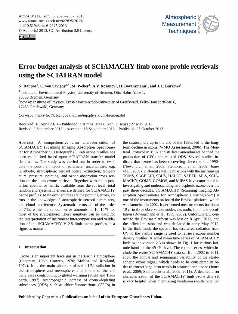
Fig. 5. Similar to Fig.2 but for the following parameters:(a) pressure,(b) tangent height, and(c) temperature sensitivity of O3 absorptioncross section (T-ozone). The viewing geometry is taken from SCIAMACHY orbit 33566 (1 August 2008) at geolocation of 70◦ N and 165◦ E,with SAA of 29◦ and SZA of 52◦.

Aerosol

-5 0 5 10 15Error [%]

0

20

40

60

80

Alti

tude

[km

]

dX: -40% 0N-30N30N-60N60N-85N

Albedo

-8 -6 -4 -2 0 2Error [%]

0

20

40

60

80

Alti

tude

[km

]

dX:+0.1 0N-30N30N-60N60N-85N

Temperature

-1.1 -1.0 -0.9 -0.8 -0.7 -0.6 -0.5Error [%]

0

20

40

60

80

Alti

tude

[km

]

dX:+2K 0N-30N30N-60N60N-85N

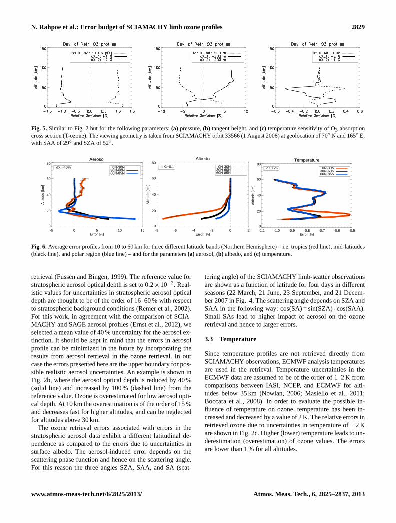
Fig. 6.Average error profiles from 10 to 60 km for three different latitude bands (Northern Hemisphere) – i.e. tropics (red line), mid-latitudes(black line), and polar region (blue line) – and for the parameters(a) aerosol,(b) albedo, and(c) temperature.

retrieval (Fussen and Bingen, 1999). The reference value forstratospheric aerosol optical depth is set to 0.2×10−2. Real-istic values for uncertainties in stratospheric aerosol opticaldepth are thought to be of the order of 16–60 % with respectto stratospheric background conditions (Remer et al., 2002).For this work, in agreement with the comparison of SCIA-MACHY and SAGE aerosol profiles (Ernst et al., 2012), weselected a mean value of 40 % uncertainty for the aerosol ex-tinction. It should be kept in mind that the errors in aerosolprofile can be minimized in the future by incorporating theresults from aerosol retrieval in the ozone retrieval. In ourcase the errors presented here are the upper boundary for pos-sible realistic aerosol uncertainties. An example is shown inFig. 2b, where the aerosol optical depth is reduced by 40 %(solid line) and increased by 100 % (dashed line) from thereference value. Ozone is overestimated for low aerosol opti-cal depth. At 10 km the overestimation is of the order of 15 %and decreases fast for higher altitudes, and can be neglectedfor altitudes above 30 km.

The ozone retrieval errors associated with errors in thestratospheric aerosol data exhibit a different latitudinal de-pendence as compared to the errors due to uncertainties insurface albedo. The aerosol-induced error depends on thescattering phase function and hence on the scattering angle.For this reason the three angles SZA, SAA, and SA (scat-

tering angle) of the SCIAMACHY limb-scatter observationsare shown as a function of latitude for four days in differentseasons (22 March, 21 June, 23 September, and 21 Decem-ber 2007 in Fig.4. The scattering angle depends on SZA andSAA in the following way: cos(SA) = sin(SZA)· cos(SAA).Small SAs lead to higher impact of aerosol on the ozoneretrieval and hence to larger errors.

3.3 Temperature

Since temperature profiles are not retrieved directly fromSCIAMACHY observations, ECMWF analysis temperaturesare used in the retrieval. Temperature uncertainties in theECMWF data are assumed to be of the order of 1–2 K fromcomparisons between IASI, NCEP, and ECMWF for alti-tudes below 35 km (Nowlan, 2006; Masiello et al., 2011;Boccara et al., 2008). In order to evaluate the possible in-fluence of temperature on ozone, temperature has been in-creased and decreased by a value of 2 K. The relative errors inretrieved ozone due to uncertainties in temperature of±2 Kare shown in Fig.2c. Higher (lower) temperature leads to un-derestimation (overestimation) of ozone values. The errorsare lower than 1 % for all altitudes.



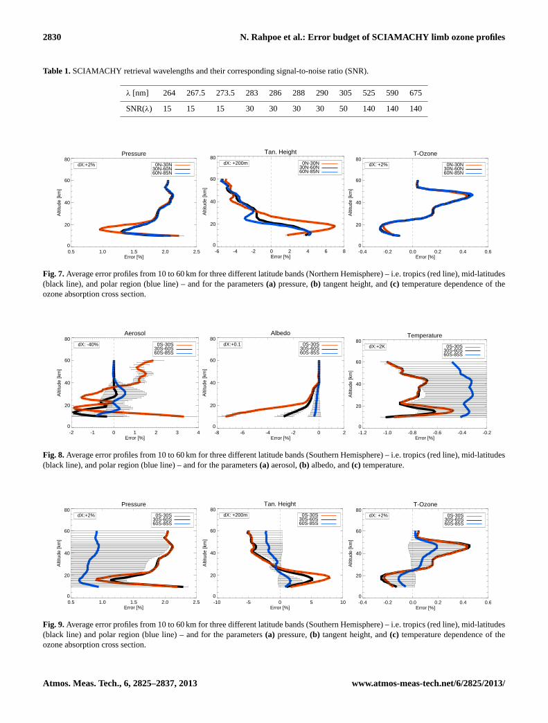
Table 1.SCIAMACHY retrieval wavelengths and their corresponding signal-to-noise ratio (SNR).

λ [nm] 264 267.5 273.5 283 286 288 290 305 525 590 675

SNR(λ) 15 15 15 30 30 30 30 50 140 140 140

Pressure

0.5 1.0 1.5 2.0 2.5Error [%]

0

20

40

60

80

Alti

tude

[km

]

dX:+2% 0N-30N30N-60N60N-85N

Tan. Height

-6 -4 -2 0 2 4 6 8Error [%]

0

20

40

60

80

Alti

tude

[km

]

dX: +200m 0N-30N30N-60N60N-85N

T-Ozone

-0.4 -0.2 0.0 0.2 0.4 0.6Error [%]

0

20

40

60

80

Alti

tude

[km

]

dX: +2% 0N-30N30N-60N60N-85N

Fig. 7.Average error profiles from 10 to 60 km for three different latitude bands (Northern Hemisphere) – i.e. tropics (red line), mid-latitudes(black line), and polar region (blue line) – and for the parameters(a) pressure,(b) tangent height, and(c) temperature dependence of theozone absorption cross section.

Aerosol

-2 -1 0 1 2 3 4Error [%]

0

20

40

60

80

Alti

tude

[km

]

dX: -40% 0S-30S30S-60S60S-85S

Albedo

-8 -6 -4 -2 0 2Error [%]

0

20

40

60

80

Alti

tude

[km

]

dX:+0.1 0S-30S30S-60S60S-85S

Temperature

-1.2 -1.0 -0.8 -0.6 -0.4 -0.2Error [%]

0

20

40

60

80

Alti

tude

[km

]dX:+2K 0S-30S

30S-60S60S-85S

Fig. 8.Average error profiles from 10 to 60 km for three different latitude bands (Southern Hemisphere) – i.e. tropics (red line), mid-latitudes(black line), and polar region (blue line) – and for the parameters(a) aerosol,(b) albedo, and(c) temperature.

Pressure

0.5 1.0 1.5 2.0 2.5Error [%]

0

20

40

60

80

Alti

tude

[km

]

dX:+2% 0S-30S30S-60S60S-85S

Tan. Height

-10 -5 0 5 10Error [%]

0

20

40

60

80

Alti

tude

[km

]

dX: +200m 0S-30S30S-60S60S-85S

T-Ozone

-0.4 -0.2 0.0 0.2 0.4 0.6Error [%]

0

20

40

60

80

Alti

tude

[km

]

dX: +2% 0S-30S30S-60S60S-85S

Fig. 9.Average error profiles from 10 to 60 km for three different latitude bands (Southern Hemisphere) – i.e. tropics (red line), mid-latitudes(black line) and polar region (blue line) – and for the parameters(a) pressure,(b) tangent height, and(c) temperature dependence of theozone absorption cross section.



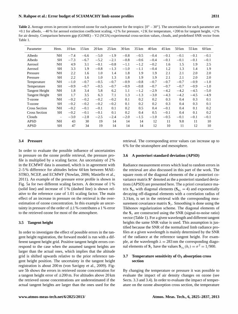
Table 2.Average errors in percent in retrieved ozone for each parameter for the tropics: [0◦ – 30◦]. The uncertainties for each parameter are+0.1 for albedo,−40 % for aerosol extinction coefficient scaling, +2 % for pressure, +2 K for temperature, +200 m for tangent height, +2 %for air density. Comparison between gpp (GOME) – V2 (SCIA) experimental cross-section values, clouds, and predefined SNR vector fromTable1.

Parameter Hem. 10 km 15 km 20 km 25 km 30 km 35 km 40 km 45 km 50 km 55 km 60 km

Albedo NH −7.4 −6.6 −5.0 −1.9 −0.8 −0.5 −0.4 −0.1 −0.1 −0.1 −0.1Albedo SH −7.3 −6.7 −5.2 −2.1 −0.8 −0.6 −0.4 −0.1 −0.1 −0.1 −0.1Aerosol NH 4.9 3.1 −0.1 −0.8 −1.1 −1.2 −0.2 1.6 1.5 1.9 2.5Aerosol SH 3.3 1.9 −0.8 −1.3 −1.0 −1.1 −0.4 1.2 1.3 1.4 1.9Pressure NH 2.2 1.6 1.0 1.4 1.8 1.9 1.9 2.1 2.1 2.0 2.0Pressure SH 2.2 1.6 1.0 1.3 1.8 1.9 1.9 2.1 2.1 2.0 2.0Temperature NH −1.0 −0.7 −0.5 −0.7 −0.9 −0.8 −0.7 −0.7 −0.7 −0.9 −1.0Temperature SH −0.9 −0.7 −0.5 −0.7 −0.9 −0.8 −0.7 −0.7 −0.7 −0.9 −1.0Tangent Height NH 1.8 3.4 5.8 6.2 1.1 −1.2 −2.9 −4.2 −4.2 −4.5 −5.0Tangent Height SH 1.7 3.5 6.3 7.1 1.3 −1.3 −3.0 −4.3 −4.2 −4.5 −4.9T-ozone NH −0.2 −0.2 −0.2 −0.2 0.1 0.2 0.2 0.3 0.4 0.3 0.1T-ozone SH −0.2 −0.2 −0.2 −0.2 0.1 0.2 0.2 0.3 0.4 0.3 0.1Cross Section NH −0.2 −0.1 −0.1 0.1 0.2 0.5 0.4 −0.1 0.4 0.1 0.2Cross Section SH −0.2 −0.1 −0.1 0.1 0.2 0.4 0.5 −0.1 0.4 0.1 0.2Clouds – −3.0 −2.8 −2.5 −2.4 −2.0 −1.5 −1.0 −0.5 −0.1 −0.1 −0.1APSD NH 43 30 19 14 14 14 12 11 9.8 11 10APSD SH 47 34 19 14 14 14 12 10 11 12 10

3.4 Pressure

In order to evaluate the possible influence of uncertaintiesin pressure on the ozone profile retrieval, the pressure pro-file is multiplied by a scaling factor. An uncertainty of 2%in the ECMWF data is assumed, which is in agreement with2–5 % difference for altitudes below 60 km between MAE-STRO, NCEP, and ECMWF (Nowlan, 2006; Masiello et al.,2011). An example of the pressure error profile is shown inFig. 5a for two different scaling factors. A decrease of 1 %(solid line) and increase of 1 % (dashed line) is shown rel-ative to the reference case of 1.01 scaling factor. The maineffect of an increase in pressure on the retrieval is the over-estimation of ozone concentration. In this example an uncer-tainty in pressure of the order of±1 % contributes a 1 % errorto the retrieved ozone for most of the atmosphere.

3.5 Tangent height

In order to investigate the effect of possible errors in the tan-gent height registration, the forward model is run with a dif-ferent tangent height grid. Positive tangent height errors cor-respond to the case when the assumed tangent heights arelarger than the actual ones, which implies that the altitudegrid is shifted upwards relative to the prior reference tan-gent height position. The uncertainty in the tangent heightregistration is about 200 m (von Savigny et al., 2009). Fig-ure5b shows the errors in retrieved ozone concentration fora tangent height error of±200 m. For altitudes above 20 kmthe retrieved ozone concentrations are underestimated if theactual tangent heights are larger than the ones used for the

retrieval. The corresponding error values can increase up to6% for the stratosphere and mesosphere.

3.6 A posteriori standard deviation (APSD)

Radiance measurement errors which lead to random errors inthe retrieval are also discussed in this part of the work. Thesquare roots of the diagonal elements of the a posteriori co-variance matrixS∗ denoted as the a posteriori standard devia-tions (APSD) are presented here. The a priori covariance ma-trix Sa, with diagonal elements (Saii

= 4) and exponentiallydecaying off-diagonal elements with a correlation radius of3.3 km, is set in the retrieval with the corresponding mea-surement covariance matrixSy . Smoothing is done using theTikhonov regularization scheme. The diagonal elements oftheSy are constructed using the SNR (signal-to-noise ratio)vector (Table1). For a given wavelength and different tangentheights the same SNR value is used. This assumption is jus-tified because the SNR of the normalized limb radiance pro-files at a given wavelength is mainly determined by the SNRof the radiance at the reference tangent height. For exam-ple, at the wavelengthλ = 283 nm the corresponding diago-nal elements ofSy have the valuesSyii

(hi) = σ 2= 1/900.

3.7 Temperature sensitivity of O3 absorption crosssection

By changing the temperature or pressure it was possible toevaluate the impact of air density changes on ozone (seeSects. 3.3 and 3.4). In order to evaluate the impact of temper-ature on the ozone absorption cross section, the temperature



Table 3.Average errors in percent for the mid-latitudes, [30◦–60◦], for the same parameters as in Table2.


Albedo NH −3.2 −2.3 −1.5 −0.8 −0.5 −0.4 −0.2 0.1 0.1 −0.1 0.1Albedo SH −2.8 −2.4 −1.7 −0.9 −0.7 −0.5 −0.4 0.1 0.1 −0.1 0.1Aerosol NH 7.6 5.4 2.9 −0.4 −1.6 −0.2 0.2 0.1 0.1 0.1 0.1Aerosol SH −0.3 −1.5 −1.7 −0.3 −0.4 0.1 0.1 0.1 0.1 0.1 0.1Pressure NH 2.0 1.5 1.3 1.6 1.8 1.9 1.9 2.1 2.1 2.1 2.0Pressure SH 2.3 1.6 1.1 1.6 1.8 1.9 1.9 2.1 2.1 2.1 2.0Temperature NH −0.9 −0.7 −0.7 −0.9 −0.9 −0.7 −0.7 −0.7 −0.7 −0.9 −1.0Temperature SH −1.0 −0.8 −0.6 −0.8 −0.8 −0.7 −0.7 −0.7 −0.7 −0.9 −1.0Tangent Height NH 3.7 4.0 3.6 1.0 −1.5 −1.6 −2.2 −3.5 −3.9 −4.9 −5.4Tangent Height SH 1.1 2.8 4.8 3.8 0.1 −1.4 −2.5 −4.0 −3.8 −4.6 −5.0T-ozone NH −0.1 −0.2 −0.2 −0.2 0.1 0.2 0.2 0.3 0.4 0.3 0.1T-ozone SH −0.1 −0.2 −0.2 −0.2 0.1 0.2 0.2 0.3 0.4 0.3 0.1Cross Section NH −0.1 −0.1 0.1 0.1 0.3 0.5 0.4 −0.1 0.4 0.1 0.2Cross Section SH −0.1 −0.1 0.1 0.1 0.3 0.5 0.5 −0.1 0.4 0.1 0.2Clouds – −3.0 −2.8 −2.5 −2.4 −2.0 −1.5 −1.0 −0.5 −0.1 −0.1 −0.1APSD NH 26 18 16 13 15 15 12 11 9.8 11 10APSD SH 33 23 17 14 14 14 12 10 11 12 10

and pressure are changed in such a way that the air densitydoes not change. Since the O3 absorption cross section de-pends only on temperature, and not on pressure, this is a suit-able way to investigate the effect of the temperature sensitiv-ity of the absorption cross section on the ozone profile re-trievals (T-ozone). Any deviation in the ozone concentrationis then a consequence of the temperature sensitivity of theozone cross section alone. The error profile due to a varia-tion of p andT is shown in Fig.5c. The temperature changeof ≈ 2 K at constant air density leads to very small errors ofup to 0.4 %, compared to the direct temperature effect (1 %)as shown in Fig. 2c.

3.8 Ozone cross section

Different laboratory measurements of the ozone absorptioncross sections are available. The Global Ozone Monitor-ing Experiment (GOME) absorption cross sections (Burrowset al., 1998) and the SCIAMACHY absorption cross-sectiondatabase (Bogumil et al., 2003) are used to estimate the un-certainties. The ozone cross-section error is here defined asthe percentage difference in the retrieved profiles using thesetwo ozone cross sections. The differences are lower than0.5 % for the entire atmosphere.

3.9 Impact of tropospheric clouds

Sonkaew et al.(2009) investigated the impact of troposphericclouds on the ozone profile retrievals assuming clouds in theforward model and performing the retrieval in a cloud-freeatmosphere. One example of their simulation, the error in thepresence of clouds with a vertical extent of 4 to 7 km andoptical thickness ofτ = 10, is included in our error budgetanalysis. TheSonkaew et al.(2009) result shows a slightly

higher sensitivity towards larger SZAs for a constant SAA.For summer conditions at 10 km the error is of the order of 3(tropics) and 5.5 % (polar latitudes), and decreases for higheraltitudes.

4 Total

Based on the error estimation for each individual parameteras a function of SCIAMACHY observation geometry, a totalerror budget can be established for the SCIAMACHY limbozone profile retrieval.

The following latitude bands with different SZAs havebeen selected for the error estimation: tropics [0–30◦], mid-latitudes [30–60◦], and polar latitudes [60–85◦]. The resultsof these calculations are summarized in Tables2–4. In Figs.6–9 the corresponding average error profiles are shown forthe following parameters: aerosol, albedo, temperature, pres-sure, tangent height, and a posteriori standard deviation forboth hemispheres. The calculation has been performed for 5different days of the year 2008 consisting of 10 orbits, with204 profiles for the Northern Hemisphere and 137 profilesfor the Southern Hemisphere. The numbers in the Tables2–4are mean uncertainties/errorsσm in percent for each param-eter (rows) and selected altitudes from 10 to 60 km averagedover 5 km altitude intervals (columns). The tables indicatethat the ozone retrievals errors caused by most of the errorsources do not exhibit strong interhemispheric differences.The only exception is stratospheric aerosols, whose effecton the ozone retrievals is significantly larger in the NorthernHemisphere at mid-latitudes. This is related to the latitudinalvariation of the SCIAMACHY limb observation geometry,which is associated with scattering angles lower than about90◦ in the Northern Hemisphere, and scattering angles larger



Pressure

0.5 1.0 1.5 2.0 2.5Error [%]

0

20

40

60

80

Alti

tude

[km

]

dX:+2% 0N-30N30N-60N60N-85N

Tan. Height

-6 -4 -2 0 2 4 6 8Error [%]

0

20

40

60

80

Alti

tude

[km

]

dX: +200m 0N-30N30N-60N60N-85N

T-Ozone

-0.4 -0.2 0.0 0.2 0.4 0.6Error [%]

0

20

40

60

80

Alti

tude

[km

]

dX: +2% 0N-30N30N-60N60N-85N



(a) pressure, (b) tangent height, and (c) T-ozone.

Aerosol

-2 -1 0 1 2 3 4Error [%]

0

20

40

60

80

Alti

tude

[km

]

dX: -40% 0S-30S30S-60S60S-85S

Albedo

-8 -6 -4 -2 0 2Error [%]

0

20

40

60

80

Alti

tude

[km

]

dX:+0.1 0S-30S30S-60S60S-85S

Temperature

-1.2 -1.0 -0.8 -0.6 -0.4 -0.2Error [%]

0

20

40

60

80

Alti

tude

[km

]

dX:+2K 0S-30S30S-60S60S-85S

Fig. 8. Average error profiles from 10–60 km for three different latitude bands (Southern Hemisphere), i.e.,

tropics (red diamond), mid latitude (solid line), and for the following parameters (a) aerosol, (b) albedo, and

(c) temperature.

Pressure

0.5 1.0 1.5 2.0 2.5Error [%]

0

20

40

60

80

Alti

tude

[km

]

dX:+2% 0S-30S30S-60S60S-85S

Tan. Height

-10 -5 0 5 10Error [%]

0

20

40

60

80

Alti

tude

[km

]

dX: +200m 0S-30S30S-60S60S-85S

T-Ozone

-0.4 -0.2 0.0 0.2 0.4 0.6Error [%]

0

20

40

60

80

Alti

tude

[km

]

dX: +2% 0S-30S30S-60S60S-85S

Fig. 9. Average error profiles from 10–60 km for three different latitude bands (Southern Hemisphere), i.e.,

tropics (red diamond), mid latitude (solid line), and for the following parameters (a) pressure, (b) tangent

height, and (c) T-ozone.

Random and systematic error profiles

0 10 20 30 40Error [%]

0

20

40

60

80

Alti

tude

[km

]

60-85 N30-60 N0-30 N

Total SystematicTotal Random

Systematic error components: [0N-30N]

0 2 4 6 8Error [%]

0

20

40

60

80

Alti

tude

[km

]

PressureTemperature

DensityCross Section

Tan. HeightAlbedoAerosolClouds

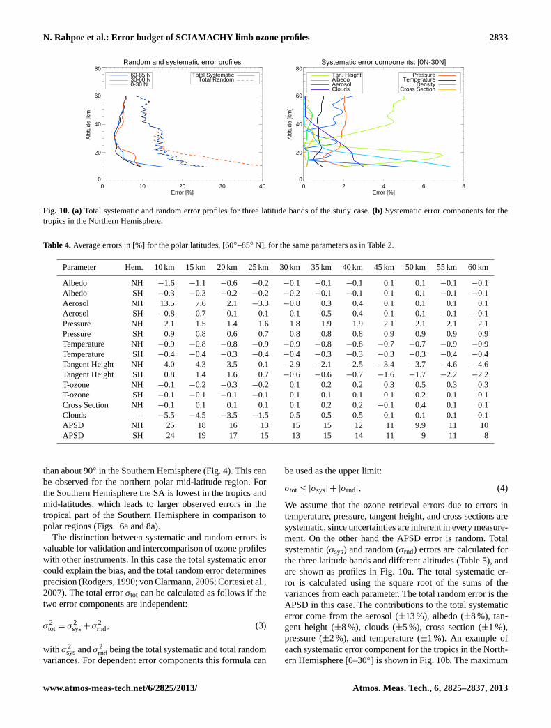
Fig. 10. (a) Total systematic and random error profiles for three latitude bands of the study case. (b) Systematic

error components for the tropics in the Northern Hemisphere.

20

Fig. 10. (a)Total systematic and random error profiles for three latitude bands of the study case.(b) Systematic error components for thetropics in the Northern Hemisphere.

Table 4.Average errors in [%] for the polar latitudes, [60◦–85◦ N], for the same parameters as in Table2.


Albedo NH −1.6 −1.1 −0.6 −0.2 −0.1 −0.1 −0.1 0.1 0.1 −0.1 −0.1Albedo SH −0.3 −0.3 −0.2 −0.2 −0.2 −0.1 −0.1 0.1 0.1 −0.1 −0.1Aerosol NH 13.5 7.6 2.1 −3.3 −0.8 0.3 0.4 0.1 0.1 0.1 0.1Aerosol SH −0.8 −0.7 0.1 0.1 0.1 0.5 0.4 0.1 0.1 −0.1 −0.1Pressure NH 2.1 1.5 1.4 1.6 1.8 1.9 1.9 2.1 2.1 2.1 2.1Pressure SH 0.9 0.8 0.6 0.7 0.8 0.8 0.8 0.9 0.9 0.9 0.9Temperature NH −0.9 −0.8 −0.8 −0.9 −0.9 −0.8 −0.8 −0.7 −0.7 −0.9 −0.9Temperature SH −0.4 −0.4 −0.3 −0.4 −0.4 −0.3 −0.3 −0.3 −0.3 −0.4 −0.4Tangent Height NH 4.0 4.3 3.5 0.1 −2.9 −2.1 −2.5 −3.4 −3.7 −4.6 −4.6Tangent Height SH 0.8 1.4 1.6 0.7 −0.6 −0.6 −0.7 −1.6 −1.7 −2.2 −2.2T-ozone NH −0.1 −0.2 −0.3 −0.2 0.1 0.2 0.2 0.3 0.5 0.3 0.3T-ozone SH −0.1 −0.1 −0.1 −0.1 0.1 0.1 0.1 0.1 0.2 0.1 0.1Cross Section NH −0.1 0.1 0.1 0.1 0.1 0.2 0.2 −0.1 0.4 0.1 0.1Clouds – −5.5 −4.5 −3.5 −1.5 0.5 0.5 0.5 0.1 0.1 0.1 0.1APSD NH 25 18 16 13 15 15 12 11 9.9 11 10APSD SH 24 19 17 15 13 15 14 11 9 11 8

than about 90◦ in the Southern Hemisphere (Fig.4). This canbe observed for the northern polar mid-latitude region. Forthe Southern Hemisphere the SA is lowest in the tropics andmid-latitudes, which leads to larger observed errors in thetropical part of the Southern Hemisphere in comparison topolar regions (Figs.6a and8a).

The distinction between systematic and random errors isvaluable for validation and intercomparison of ozone profileswith other instruments. In this case the total systematic errorcould explain the bias, and the total random error determinesprecision (Rodgers, 1990; von Clarmann, 2006; Cortesi et al.,2007). The total errorσtot can be calculated as follows if thetwo error components are independent:

σ 2tot = σ 2

sys+ σ 2rnd, (3)

with σ 2sysandσ 2

rnd being the total systematic and total randomvariances. For dependent error components this formula can

be used as the upper limit:

σtot ≤ |σsys| + |σrnd|, (4)

We assume that the ozone retrieval errors due to errors intemperature, pressure, tangent height, and cross sections aresystematic, since uncertainties are inherent in every measure-ment. On the other hand the APSD error is random. Totalsystematic (σsys) and random (σrnd) errors are calculated forthe three latitude bands and different altitudes (Table5), andare shown as profiles in Fig.10a. The total systematic er-ror is calculated using the square root of the sums of thevariances from each parameter. The total random error is theAPSD in this case. The contributions to the total systematicerror come from the aerosol (±13 %), albedo (±8 %), tan-gent height (±8 %), clouds (±5 %), cross section (±1 %),pressure (±2 %), and temperature (±1 %). An example ofeach systematic error component for the tropics in the North-ern Hemisphere [0–30◦] is shown in Fig.10b. The maximum



Table 5.Total error±σtot in [%] for the three different latitude bands for both hemispheres (NH/SH) separated into total systematic and totalrandom uncertainties for tropics, 0◦–30◦; mid-latitudes, 30◦–60◦; and polar region, 60◦–85◦.

Lat. Band 10 km 15 km 20 km 25 km 30 km 35 km 40 km 45 km 50 km 55 km 60 km

Total Systematic

NH: Tropics 9 8 8 7 3 3 3 5 5 5 6NH: Midlat. 9 7 5 3 3 3 3 4 4 5 5NH: Polar 15 10 6 5 3 2 3 4 4 5 5SH: Tropics 9 8 8 8 3 3 3 4 4 5 5SH: Midlat. 4 5 6 4 2 2 3 4 4 5 5SH: Polar 5 5 4 3 1 1 1 1 2 2 2

Total Random

NH: Tropics 43 30 19 13 14 14 12 10 11 12 10NH: Midlat. 26 18 16 13 15 15 12 10 11 11 10NH: Polar 25 18 16 13 15 15 12 11 10 11 10SH: Tropics 47 34 19 14 14 14 12 10 10 12 10SH: Midlat. 33 23 17 14 14 14 12 10 11 12 10SH: Polar 42 26 21 19 20 21 21 15 20 19 18

random error is of the order of±34 % in the tropics at 15 km,and decreases down to 12 % for higher altitudes in the North-ern Hemisphere. The values of the random error componentare systematically higher for the Southern Hemisphere.

5 Discussion

The sensitivity study presented here shows similar resultscompared to sensitivity studies performed for SAGE III(Rault and Taha, 2007) and MLS (Froidevaux et al., 2008).In both studies, precision and accuracy have been estimatedusing a similar method. For SAGE III limb-scatter measure-ments, the instrument error in stratospheric ozone caused byalbedo errors (surface reflectance) has been estimated to beof the order of 3 % for the altitude range of 20–30 km. Inthe study byRault and Taha(2007) a surface reflectancechange of 0.45 has been used, which can lead to a 13 % er-ror at 15 km. In our study the error is of the order of 6 %for an albedo perturbation of 0.1 in the tropics at 15 km.The same study reveals a 6 % error around 20 km when thestratospheric aerosol are neglected. Our calculation of 40 %aerosol perturbation relative to the background state leads toa 2.9 % error at 20 km in northern mid-latitudes, decreasingfast with increasing altitude (see Table3). The third commonparameter used for the study is the tangent height. In SAGEIII an offset of 350 m has been used, which leads to errorsof the order of 5 % and a peak error value of 12 % at 15 km.Our study reveals an error of 4 % above 30 km with a peakaround 20 km of the order of 6 % for an offset of 200 m. Fortemperature the sensitivity study of MLS V 2.2 performed byFroidevaux et al.(2008) can be used. The effect of temper-ature uncertainties on ozone retrievals in the microwave andUV–visible range may be entirely different, and as such ourresults cannot be directly compared to the MLS values. The

temperature induced error is of the order of 2 % and is con-sistent with our results. In the same study the impact of ra-diometric knowledge and spectroscopy have been evaluatedas of the order of 2 % in the stratosphere. Stray light and po-larization effects can add up to the total error budget as well.Neglecting these additional parameters can lead to underes-timation of the total error budget. Polarization is altitude de-pendent, and due to the normalization scheme used for ozoneretrieval, the altitude dependence of polarization and the dif-ferential structure of polarization can influence the scatteringprocess. The differential structure in polarization is of the or-der of 0.1, which leads to a 1–2 % effect on single scattering.

6 Conclusions

The SCIATRAN radiation transfer code has been used in or-der to determine the sensitivity of ozone profile retrievalsfrom SCIAMACHY limb-scatter measurements to eight pa-rameters known to provide a potentially major contributionto SCIAMACHY limb ozone profile retrieval errors. The rel-ative deviations have been estimated for realistic uncertain-ties for individual parameters. The results of the sensitivitystudy indicate that the total systematic error is dominatedby aerosol and albedo for altitudes below 20 km, i.e. up to±13 % for aerosol at the northern polar latitudes and±7 %for albedo in the tropics at 10 km altitude. The ozone re-trieval errors associated with errors in tangent height, clouds,and pressure dominate the total systematic error for altitudesabove 20 km and can lead to total systematic errors of theorder of±5 % at these altitudes. The contribution of uncer-tainties in temperature, the choice of ozone absorption crosssection, and the temperature dependence of the ozone ab-sorption cross section (T-ozone) to the total systematic er-ror can be neglected. The random error is the a posteriori



covariance standard deviation (APSD) for a defined SNR inour case. The total random error in the Northern Hemisphereranges between±34 (15 km, tropics) and±12 % (40 km,polar region).

The total systematic and total random errors have beendefined and calculated for the tropics, mid-latitudes, andpolar latitudes. The total systematic error for the altitudesabove 15 km is below 5, 5, and 8 % in the polar region, mid-latitudes, and tropics, respectively.

The total error budget is underestimated by neglectingthe radiometric, spectroscopic, stray-light, and polarizationeffects on the ozone retrieval.

Our results indicate that incorrect knowledge of aerosolloading and surface albedo can affect the ozone profile re-trievals dramatically for altitudes below 20 km. Determina-tion of exact tangent height is crucial, since any small uncer-tainty in the knowledge of tangent height can lead to fairlylarge systematic ozone deviations. The effects of pressureand temperature have to be considered with care for long-term ozone trends, where systematic trends in the thermody-namic parameters can impact the derived long-term trends.

The results of our analysis can be used as total error limits(systematic = bias; random = precision) for validation and in-tercomparison tasks of SCIAMACHY ozone data with otherconcurrent instruments. The use of total error budget is im-portant, especially for long-term investigations of ozone be-haviour in a changing climate or validation between differentinstruments.

Acknowledgement.This work has been funded within the frame-work of the ESA project OZONE CCI (Climate Change Initiative).We would like to thank the SCIAMACHY and SCIATRAN groupfor providing the data and tools for this work. The suggestions andcomments made by an anonymous referee and Douglas Degensteinhave improved the paper, and we would like to thank them for theircontribution.

Edited by: R. Eckman

References

Barker, H. W. and Davies, J. A.: Surface albedo estimates fromNimbus-7 ERB Data and a two-stream approximation of the ra-diative transfer equation, J. Climate, 2, 409–418, 1989.

Boccara, G., Hertzog, A., Basdevant, C., and Vial, F.: Accuracyof NCEP/NCAR reanalyses and ECMWF analyses in th lowerstratosphere over Antarctica in 2005, J. Geophys. Res., 113,D20115, doi:10.1029/2008JD010116, 2008.

Bogumil, K., Orphal, J., Homann, T., Voigt, S., Spietz, P., Fleis-chmann, O. C., Vogel, A., Hartmann, M., Bovensmann, H., Fr-erick, J., and Burrows, J. P.: Measurements of molecular ab-sorption spectra with the SCIAMACHY pre-flight model: instru-ment characterisation and reference data for atmospheric remote-sensing in the 230–2380 nm region, J. Photochem. Photobio. A.,157, 157–167, 2003.

Bovensmann, H., Burrows, J. P., Buchwitz, M., Frerick, J., Noël, S.,Rozanov, V. V., Chance, K. V., and Goede, A. P. H.: SCIA-MACHY: mission objectives and measurement modes, J. Atmos.Sci., 56, 127–150, 1999.

Bovensmann, H., Ahlers, B., Buchwitz, M., Frerick, J.,Gottwald, M., Hoogeveen, R., Kaiser, J. W., Kleipool, Q.,Krieg, E., Lichtenberg, G., Mager, R., Meyer, J., Noël, S., Schle-sier, A., Sioris, C., Skupin, J., von Savigny, C., Wuttke, M. W.,and Burrows, J. P.: SCIAMACHY in-flight instrument perfor-mance, Proceedings of the Envisat Calibration Review (SP-520),ESA Publications Division, Frascati, Italy, 9–13 December,2002.

Bracher, A., Bovensmann, H., Bramstedt, K., Burrows, J. P., vonClarmann, T., Eichmann, K.-U., Fischer, H., Funke, B., Gil-Lopez, S., Glatthor, N., Grabowski, U., Höpfner, M., Kauf-mann, M., Kellmann, S., Kiefer, M., Koukouli, M. E., Linden, A.,Lopez-Puertas, M., Mengistu Tsidu, G., Milz, M., Noël, S., Ro-hen, G., Rozanov, A., Rozanov, V. V., von Savigny, C., Sinnhu-ber, M., Skupin, J., Steck, T., Stiller, G. P., Wang, D.-Y., We-ber, M., and Wuttke, M. W.: Cross comparisons of O3 andNO2 measured by the atmospheric ENVISAT instruments GO-MOS, MIPAS, and SCIAMACHY, Adv. Space Res., 36, 855–867, doi:10.1016/j.asr.2005.04.005, 2005.

Burrows, J. P., Richter, A., Dehn, A., Deters, B., Himmelmann, S.,Voigt, S., and Orphal, J.: Atmospheric remote-sensing referencedata from GOME: 2. temperature-dependent absorption crosssections of O3 in the 231–794 nm range, J. Quant. Spectrosc. Ra-diat. Transfer, 61, 509–517, 1998.

Butz, A., Bösch, H., Camy-Peyret, C., Chipperfield, M., Dorf, M.,Dufour, G., Grunow, K., Jeseck, P., Kühl, S., Payan, S., Pepin, I.,Pukite, J., Rozanov, A., von Savigny, C., Sioris, C., Wagner, T.,Weidner, F., and Pfeilsticker, K.: Inter-comparison of strato-spheric O3 and NO2 abundances retrieved from balloon borne di-rect sun observations and Envisat/SCIAMACHY limb measure-ments, Atmos. Chem. Phys., 6, 1293–1314, doi:10.5194/acp-6-1293-2006, 2006.

Chapman, S.: A theory of upper-atmospheric ozone, Mem. R.Metrol. Soc., 3, 103–125, 1930.

Cortesi, U., Lambert, J. C., De Clercq, C., Bianchini, G., Blumen-stock, T., Bracher, A., Castelli, E., Catoire, V., Chance, K. V.,De Mazière, M., Demoulin, P., Godin-Beekmann, S., Jones, N.,Jucks, K., Keim, C., Kerzenmacher, T., Kuellmann, H., Kut-tippurath, J., Iarlori, M., Liu, G. Y., Liu, Y., McDermid, I. S.,Meijer, Y. J., Mencaraglia, F., Mikuteit, S., Oelhaf, H.,Piccolo, C., Pirre, M., Raspollini, P., Ravegnani, F., Re-burn, W. J., Redaelli, G., Remedios, J. J., Sembhi, H., Smale, D.,Steck, T., Taddei, A., Varotsos, C., Vigouroux, C., Waterfall, A.,Wetzel, G., and Wood, S.: Geophysical validation of MIPAS-ENVISAT operational ozone data, Atmos. Chem. Phys., 7, 4807–4867, doi:10.5194/acp-7-4807-2007, 2007.

Crutzen, P. J.: The influence of nitrogen oxides on the atmosphericozone content, Q. J. Roy. Meteor. Soc., 96, 320–325, 1970.

Ernst, F., von Savigny, C., Rozanov, A., Rozanov, V., Eichmann, K.-U., Brinkhoff, L. A., Bovensmann, H., and Burrows, J. P.: Globalstratospheric aerosol extinction profile retrievals from SCIA-MACHY limb-scatter observations, Atmos. Meas. Tech. Dis-cuss., 5, 5993–6035, doi:10.5194/amtd-5-5993-2012, 2012.


http://dx.doi.org/10.1029/2008JD010116

http://dx.doi.org/10.1016/j.asr.2005.04.005

http://dx.doi.org/10.5194/acp-6-1293-2006



http://dx.doi.org/10.5194/amtd-5-5993-2012


Flittner, D. E., Bhartia, P. K., and Herman, B. M.: Ozone profilesretrieved from limb scatter measurements: theory, Geophys. Res.Lett., 27, 2601–2604, 2000.

Froidevaux, L., Jiang, Y. B., Lambert, A., Livesey, N. J., Read,W. G., Waters, W., Browell, E. V., Hair, J. W., Avery, M. A.,McGee, T. J, Twigg, L. W., Sumnicht, K. W., Margitan, J. J.,Sen, B., Stachnik, R. A., Toon, G. C., Bernath, P. F., Boone,C. D., Walker, K. A., Filipiak, M. J., Harwood, R. S., Fuller,R. A., Manney, G. L., Schwartz, M. J., Daffer, W. H., Drouin,B. J., Cofield, R. E., Cuddy, D. T., Jarnot, R. F., Knosp, B. W.,Perun, V. S., Snyder, W. V., Stek, P. C., Thurstans, R. P., andWagner, P. A.: Validation of Aura Microwave Limb Sounderstratospheric ozone measurements, J. Geophys. Res., Vol. 113,D15S20, doi:10.1029/2007JD008771, 2008.

Fussen, D. and Bingen, C.: A volcanism dependent model forthe extinction profile of stratospheric aerosols in the UV-visiblerange, Geophys. Res. Lett., 26, 703–706, 1999.

Hendrick, F., Van Roozendael, M., Kylling, A., Petritoli, A.,Rozanov, A., Sanghavi, S., Schofield, R., von Friedeburg, C.,Wagner, T., Wittrock, F., Fonteyn, D., and De Mazière, M.: In-tercomparison exercise between different radiative transfer mod-els used for the interpretation of ground-based zenith-sky andmulti-axis DOAS observations, Atmos. Chem. Phys., 6, 93–108,doi:10.5194/acp-6-93-2006, 2006.

Jones, A., Urban, J., Murtagh, D. P., Eriksson, P., Brohede, S.,Haley, C., Degenstein, D., Bourassa, A., von Savigny, C.,Sonkaew, T., Rozanov, A., Bovensmann, H., and Burrows, J.:Evolution of stratospheric ozone and water vapour time seriesstudied with satellite measurements, Atmos. Chem. Phys., 9,6055–6075, doi::10.5194/acp-9-6055-2009, 2009.

Kiehl, J. T. and Trenberth, K. E.: Earth’s annual global mean energybudget, B. Am. Meteor. Soc., 78, 197–208, 1997.

Kurosu, T., Rozanov, V. V., and Burrows, J. P.: Parameteriza-tion schemes for terrestrial water clouds in the radiative trans-fer model GOMETRAN, J. Geophys. Res., 102, 21809–21823,1997.

Loughman, R. P., Griffioen, E., Oikarinen, L., Postylyakov, O. V.,Rozanov, A., Flittner, D. E., and Rault, D. F.: Compar-ison of radiative transfer models for limb-viewing scat-tered sunlight measurements, J. Geophys. Res., 109, D06303,doi:10.1029/2003JD003857, 2004.

Masiello, G., Matricardi, M., and Serio, C.: The use of IASI datato identify systematic errors in the ECMWF forecasts of temper-ature in the upper stratosphere, Atmos. Chem. Phys., 11, 1009–1021, doi:10.5194/acp-11-1009-2011, 2011.

Matthews, E.: Global vegetation and land use: new high resolutiondata bases for climate studies, J. Appl. Meteorol., 22, 474–487,1983.

Mieruch, S., Weber, M., von Savigny, C., Rozanov, A., Bovens-mann, H., Burrows, J. P., Bernath, P. F., Boone, C. D., Froide-vaux, L., Gordley, L. L., Mlynczak, M. G., Russell III, J. M.,Thomason, L. W., Walker, K. A., and Zawodny, J. M.: Globaland long-term comparison of SCIAMACHY limb ozone profileswith correlative satellite data (2002–2008), Atmos. Meas. Tech.,5, 771–788, doi:10.5194/amt-5-771-2012, 2012.

Molina, M. and Rowland, F.: Stratospheric sinks for cholorfluo-romethanes: chlorine atom-catalyzed destruction of ozone, Na-ture, 249, 810–812, 1974.

Newchurch, M. J., Yang, E. S., Cunnold, D. M., Reinsel, G. C., Za-wodny, J. M., and Russell III, J. M.: Evidence for slowdown instratospheric ozone loss: first stage of ozone recovery, J. Geo-phys. Res., 108, 4507, doi:10.1029/2003JD003471, 2003.

Nowlan, R. C.: Atmospheric Temperature and Pressure Measure-ments from the ACE-MAESTRO Space Instrument, Ph.D. The-sis, University of Toronto, Toronto, Canada, 2006.

Rault, D. F., and Taha, G.: Validation of ozone profiles re-trieved from Stratospheric Aerosol and Gas Experiment III limbscatter measurements, J. Geophys. Res., Vol. 112, D13309,doi:10.1029/2006JD007679, 2007.

Remer, L. A., Kaufman, Y. J., Levin, Z., and Ghan, S.: Model as-sessment of the ability of MODIS to measure top-of-atmospheredirect radiative forcing from smoke aerosols, J. Atmos. Sci., 59,657–667, 2002.

Rodgers, C. D.: Characterization and error analysis of profiles re-trieved from remote sounding measurements, J. Geophys. Res.,95, 5587–5595, 1990.

Rozanov, A., Rozanov, V. V., and Burrows, J. P.: A numerical radia-tive transfer model for a spherical planetary atmosphere: com-bined differential-integral approach involving the Picard iterativeapproximation, J. Quant. Spectrosc. Ra., 69, 491–512, 2001.

Rozanov, A., Bovensmann, H., Bracher, A., Hrechanyy, S.,Rozanov, V. V., Sinnhuber, M., Stroh, F., and Burrows, J. P.:NO2 and BrO2 vertical profile retrieval from SCIAMACHY limbmeasurements: sensitivity studies, Adv. Space Res., 36, 846–854,doi:10.1016/j.asr.2005.03.013, 2005a.

Rozanov, A., Rozanov, V. V., Buchwitz, M., Kokhanovsky, A., andBurrows, J. P.: SCIATRAN 2.0 – a new radiative transfer modelfor geophysical applications in the 175–2400 nm spectral region,Adv. Space Res., 36, 1015–1019, 2005b.

Rozanov, A., Eichmann, K.-U., von Savigny, C., Bovensmann, H.,Burrows, J. P., von Bargen, A., Doicu, A., Hilgers, S., Godin-Beekmann, S., Leblanc, T., and McDermid, I. S.: Comparisonof the inversion algorithms applied to the ozone vertical profileretrieval from SCIAMACHY limb measurements, Atmos. Chem.Phys., 7, 4763–4779, doi:10.5194/acp-7-4763-2007, 2007.

Rozanov, V. V. and Kokhanovsky, A. A.: Determination of cloudgeometrical thickness using backscattered solar light in a gaseousabsorption band, IEEE Geosci. Remote S., 3, 250–253, 2006.

Rozanov, V. V. and Kokhanovsky, A. A.: Impact of single- andmulti-layered cloudiness on ozone vertical column retrievals us-ing nadir observations of backscattered solar radiation, in: LightScattering Reviews 3, Springer, Praxis Publishing, Chichester,UK, 133–189, 2008.

Rozanov, V. V., Diebel, D., Spurr, R., and Burrows, J. P.: GOME-TRAN: a radiative transfer model for the satellite project GOME– the plane-parallel version, J. Geophys. Res., 102, 16683–16695, 1997.

Siewert, C. E.: A discrete-ordinates solution for radiative-transfermodels that include polarization effects, J. Quant. Spectrosc. Ra.,64, 227–254, 2000.

Sonkaew, T., Rozanov, V. V., von Savigny, C., Rozanov, A., Bovens-mann, H., and Burrows, J. P.: Cloud sensitivity studies for strato-spheric and lower mesospheric ozone profile retrievals from mea-surements of limb-scattered solar radiation, Atmos. Meas. Tech.,2, 653–678, doi:10.5194/amt-2-653-2009, 2009.

Steinbrecht, W., Claude, H., Schönborn, F., McDermid, I. S.,Leblanc, T., Godin-Beekmann, S., Keckhut, P., Hauchecorne, A.,


http://dx.doi.org/10.1029/2007JD008771


http://dx.doi.org/:

http://dx.doi.org/10.1029/2003JD003857


http://dx.doi.org/10.5194/amt-5-771-2012

http://dx.doi.org/10.1029/2003JD003471

http://dx.doi.org/10.1029/2006JD007679

http://dx.doi.org/10.1016/j.asr.2005.03.013


http://dx.doi.org/10.5194/amt-2-653-2009


Gijsel, J. A. E. V., Swart, D. P. J., Bodeker, G. E., Par-rish, A., Boyd, I. S., Kämpfer, N., Hocke, K., Stolarski, R. S.,Frith, S. M., Thomason, L. W., Remsberg, E. E., von Savigny, C.,Rozanov, A., and Burrows, J. P.: Ozone and temperature trends inthe upper stratosphere at five stations of the network for the de-tection of atmospheric composition change, Int. J. Remote Sens.,30, 3875–3886, 2009.

Steinbrecht, W., Köhler, U., Claude, H., Weber, M., Burrows, J. P.,and van der A, R. J.: Very high ozone columns at north-ern mid-latitudes in 2010, Geophys. Res. Lett., 38, L06803,doi:10.1029/2010GL046634, 2011.

von Clarmann, T.: Validation of remotely sensed profiles of atmo-spheric state variables: strategies and terminology, Atmos. Chem.Phys., 6, 4311–4320, doi:10.5194/acp-6-4311-2006, 2006.

von Savigny, C., Haley, C. S., Sioris, C. E., McDade, I. C.,Llewellyn, E. J., Degenstein, D., Evans, W. F. J., Gattinger, R. L.,Griffioen, E., Kyrölä, E., Lloyd, N. D., McConnell, J. C.,McLinden, C. A., Mégie, G., Murtagh, D. P., Solheim, B., andStrong, K.: Stratospheric ozone profiles retrieved from limb scat-tered sunlight radiance spectra measured by the OSIRIS in-strument on the Odin satellite, Geophys. Res. Lett., 30, 1755,doi:10.1029/2002GL016401, 2003.

von Savigny, C., Rozanov, A., Bovensmann, H., Eichmann, K.-U.,Noël, S., Rozanov, V. V., Sinnhuber, B.-M., Weber, M., Bur-rows, J. P., and Kaiser, J. W.: The ozone hole breakup in septem-ber 2002 as seen by SCIAMACHY on ENVISAT, J. Atmos. Sci.,62, 721–734, 2005a.

von Savigny, C., McDade, I. C., Griffioen, E., Haley, C. S.,Sioris, C. E., and Llewellyn, E. J.: Sensitivity studies andfirst validation of stratospheric ozone profile retrievals fromOdin/OSIRIS observations of limb-scattered solar radiation,Can. J. Phys., 83, 9, 957–972, 2005b.

von Savigny, C., Bovensmann, H., Bramstedt, K., Dikty, S., Ebo-jie, F., Jones, A., Noël, S., Rozanov, A., and Sinnhuber, B.-M.:Indications for long-term trends and seasonal variations in theSCIAMACHY Level 1 version 6.03 tangent height information,Techn. Note IUP scia pointing 2009-01, Issue 2, University ofBremen, Bremen, Germany, 2009.

Wagner, T., Burrows, J. P., Deutschmann, T., Dix, B., von Friede-burg, C., Frieß, U., Hendrick, F., Heue, K.-P., Irie, H.,Iwabuchi, H., Kanaya, Y., Keller, J., McLinden, C. A., Oetjen, H.,Palazzi, E., Petritoli, A., Platt, U., Postylyakov, O., Pukite, J.,Richter, A., van Roozendael, M., Rozanov, A., Rozanov, V., Sin-reich, R., Sanghavi, S., and Wittrock, F.: Comparison of box-air-mass-factors and radiances for Multiple-Axis Differential Opti-cal Absorption Spectroscopy (MAX-DOAS) geometries calcu-lated from different UV/visible radiative transfer models, At-mos. Chem. Phys., 7, 1809–1833, doi:10.5194/acp-7-1809-2007,2007.

WMO: Assessment, Scientific Assessment of Ozone Depletion:2006, 50, World Meteorological Organization, Geneva, Switzer-land, 2006.


http://dx.doi.org/10.1029/2010GL046634


http://dx.doi.org/10.1029/2002GL016401


measurement error budget analysis of sciamachy limb ozone

Documents