measurement and modeling of the 3-d solar irradiance for
TRANSCRIPT
Article
Measurement and modeling of the 3-D solar
irradiance for vehicle-integrated photovoltaic Kenji Araki 1,*, Yasuyuki Ota 2, and Masafumi Yamaguchi 1
1 Toyota Technological Institute, Nagoya 468-8511, Japan; [email protected] 2 Organization for Promotion of Tenure Track, University of Miyazaki, Miyazaki 889-2192, Japan; y-
* Correspondence: [email protected]; Tel.: +81-52-809-1830
Featured Application: This technology is expected to be applied to vehicle-integrated
photovoltaic.
Abstract: The energy yield of the Vehicle-integrated photovoltaic (VIPV) differs from that of the standard
photovoltaics (PV). It is mainly by the difference of the solar irradiance onto the car-roof and car-bodies as well
as its curved-shape. Both meaningful and practical modeling and measurement of the solar irradiance for VIPV
are needed to be newly established, not the extension of the current technologies. The solar irradiance was
modeled by a random distribution of the shading objects and car-orientation with the correction of the curved
surface of the PV modules. The measurement of the solar irradiance onto the car-roof and car-body was done
using five pyranometers in five local axes on the car for one year. The measured dynamic solar irradiance onto
the car-body and car-roof was used for validation of the solar irradiance model in the car.
Keywords: photovoltaic; EV; PHV; standardization; car-roof; flexible PV; performance modeling;
rating
1. Introduction
Let us think about a solar-engine car, by the recent development and prevail of EV (Electric vehicle)
and PHV (Plug-in hybrid vehicle). The PV technologies will be game-changing in the automobile
industry. It may be a dream now, but it is worth challenging [1].
The case study of the photovoltaic (PV) driven cars was conducted both by car manufacturers [2]
and a think tank [3], and both reached the same conclusion in 2017. About 70 % of a vehicle can run
exclusively by solar energy [2-3]. The calculation base was published, namely: projected area of PV is
3.23 m2, temperature loss is 9 %, MPPT loss is 5 %, DC-DC converter loss is 10 %, battery charging and
discharging loss is 5 %, Electronic Control Unit (ECU) loss is 0.12 kWh/day, mileage is 12.5 km/kWh to
Electric Vehicles (EV), 10 km/kWh to Plug-in Hybrid Vehicles (PHV), and the battery size is 40 kWh to
EV and 10 kWh to PHV. Then, the requirement of the car-roof PV will be 1 kW. As a result, 70 % of the
cars (runs less than 30 km/day) are expected to run by solar energy [2-4]. When we multiply 71 million
vehicles (annual sales in 2017), the expected sales will be 50 GW/year [1, 5]. The above calculations
assume that the solar cells are stabilized and no or negligible degradation. However, some solar cells
degrade by time, and it is to be considered, in case such type of solar cells are used [6-9]. The
photovoltaic is also useful for auxiliary powers and range-extension of other low-carbon energies [10-
15]
The efficiency and power rating, as well as energy prediction under the curved surface affected by
the shading objects, are critical. For example, the car-roof is three-dimensionally curved, and its
curvature may induce power loss by increased cosine loss and self-shading loss [1, 16-20]. The
Preprints (www.preprints.org) | NOT PEER-REVIEWED | Posted: 15 January 2020 doi:10.20944/preprints202001.0018.v2
© 2020 by the author(s). Distributed under a Creative Commons CC BY license.
Peer-reviewed version available at Appl. Sci. 2020, 10, 872; doi:10.3390/app10030872

2 of 25
irradiance and temperature of the car-roof are different from that of the roof-top or the ground
mounting systems [16]. The expected energy yield should be different.
Car roofs are often shaded, resulting in significant losses by the string mismatching [1]. It may be
improved by the introduction of a power distribution circuit for compensating the mismatch [16, 21-
23]. However, due to the limited area and allowed thickness on the car-roof, the most practical approach
is increasing the number of series-connected strings [24].
Another aspect is that the car-roof PV is not in the installation of the standard slope angle and
orientation. The orientation of the car-roof changes by time without correlation to the sun direction.
Surrounded buildings and other objects (trees and signals) often shade PV panels, and the variety of
the curved shape has a complicated impact. Such interaction is needed to take into account [1].
The development of meaningful testing and modeling methods were done by the international
group using a web-meeting [16-19]. The 3-D model of photovoltaic power generation developed
initially in the car-roof PV, namely VIPV (Vehicle integrated photovoltaic), can be extended to VIPV
applications with curved PV using a flexible one.
This article covers the modeling and measurement of the solar-irradiance of the car-body for
accurate, meaningful, and non-biased estimation of the energy yield of automobile mounting PV
modules.
2. Model
With the progress of the automotive technology, it will help to cover the limited power output of
the car-roof PV so that most of the private cars will be able to run by solar energy equipped with high-
efficiency and 3-D curved solar panels [1-3], and will overcome the loss mentioned above. To do so, the
conventional IEC 60904 international standard series for PV electrical characterization, now focusing
on 2-D flat panels, will need to expand to 3-D shaped PV modules [1, 5, 16-20]. We attempt to define
3-D solar irradiation and rating to the 3-D curved solar panels. We also have to consider the cross effect
between the 3-D curved surface of the PV module and 3-D solar irradiance around the module [24-26].
The standard PV modules are installed to avoid shadows. However, the car-roof PV is not
orientated for the utilization of solar energy. The driver’s convenience often shades the PV. The relative
orientation of the PV on the car to the sun position is not fixed but frequently changes by driving. The
PV on the car body and the car roof are curved. It often shaded by its surfaces. Therefore, the scale of
performance is to be reconstructed.
The position and height of the shading objects are often difficult to predict. For predicting the total
solar energy to a vehicle (either annual or monthly basis) in a specific area, not in a particular driving
course, it is convenient to predict the shading influence using rough indicators of the roughness of the
land. The value of the annual or monthly solar irradiance value in a specific area is valuable to predict
the driving performance of vehicles mounting the PV panel.
We have to consider the following car-specific issues.
1. More chance of shading by objects around the car (trees and buildings)
2. Curved surface
3. The orientation angle randomly varies.
4. Mismatching loss by partial shading
2.1. Shading probability
The shading influence is complicated and varies by the position and the relative orientation (to the
sun position) of the panel. In the case of the car-roof PV, the position (orientation) of the panel cannot
be predicted. One practical approach is to rely on the probability model, supposing that some statistical
model randomly distributes the distribution of height and density of the shading objects, and the
orientation of the car is independent and random as well.
Assuming the segmented annular region, and the building or other shading objects are randomly
distributed in this region with random height (Figure 1), the probability of the shading can be
approximated as linear relationship [24, 26], because the height of the shading object is assumed to be
Preprints (www.preprints.org) | NOT PEER-REVIEWED | Posted: 15 January 2020 doi:10.20944/preprints202001.0018.v2
Peer-reviewed version available at Appl. Sci. 2020, 10, 872; doi:10.3390/app10030872

3 of 25
inversely proportional to the distance from the car, whereas the number of the shading objects along
the arc of the given distance is proportional to the distance from the car so that the product of two
factors will be the constant value (Figure 2). Note it is convenient to represent the height of the
surrounding buildings and other shading objects scaling by the shading angle (grazing angle) [24, 26].
Supposing the height of the shading object (represented by shading angle, namely, grazing angle)
is distributed by the ranged uniform distribution, the accumulated distribution as a function of the
shading angle (grazing angle) is calculated as a ranged integral so that the general trend is a linear
starting one at zero degrees of the shading angle (grazing angle). It is also important to note that the
distribution of the shading objects to the car and building is not axially symmetry and different in the
direction to the parallel to the road and orthogonal to the road. Typically, the shading probability of the
car-roof PV along the road is less than that of the orthogonal direction of the road in the local coordinate.
The area of the segmented annular is convenient to model such a situation (Figure 1) [24, 26]. Note that
the annular in place of the disk should be considered to avoid the situation of “division by zero” in
angle calculation [24, 26]. Also note that the line slope varies in two directions, one is along the road,
and another is orthogonal to the road [24, 26]. A single parameter can represent this trend. Namely,
average shading height, corresponding to the 50 % of probability of shading [24, 26].
Figure 1. Illustration of the segmented annular region for modeling distribution of the shading objects
around the PV panel.
Figure 2. The distribution curve of the shading probability used to the model.
2.2. 3-D irradiance model
For modeling the solar irradiance of the car-roof, we assumed a simple shading and scattering
reflection model. The entire shading objects were assumed that the reflectance was 0.25, and
reflection is Lambertian. Both direct and scattered solar irradiance were assumed to be shaded by the
Average shading heights
Sh
ad
ing p
rob
ab
ility
0
0.5
1 X-direction
Y-direction
Preprints (www.preprints.org) | NOT PEER-REVIEWED | Posted: 15 January 2020 doi:10.20944/preprints202001.0018.v2
Peer-reviewed version available at Appl. Sci. 2020, 10, 872; doi:10.3390/app10030872

4 of 25
shading objects as a function of the sun-height and DNI (direct normal irradiance). The probability
of the shading event calculated the shading probability and solid angle.
Assuming that the diffused irradiance from the unshaded sky is uniform, the factor of the
diffused sunlight relative to the unshaded sky was approximated by the equation (1) using random
numbers. Note that the shape of buildings and other shading objects are rectangular, and they are
not spherical triangles or spherical trapezoids. It is realistic to model it as a cylinder sky using
equation (1).
𝛔𝐬(𝜃ℎ) = 1 − (1 − 𝑅𝑏) (𝜃ℎ
90°⁄ ) (1)
where, 𝛔𝐬(𝑥) is a function of the ratio of the diffused sunlight from the sky excluding the reflection
of the direct sunlight to the shading objects, 𝑅𝑏 is the reflectance of the shading objects (fixed to 0.25
in this calculation), 𝜃ℎ is the average height of the shading objects scaled by the grazing angle (note
that the maximum angle is 45°in this model).
The direct sunlight was approximated by Equation (2).
𝛔𝒅(𝜂, 𝜃ℎ) = [
0 (𝜂 < 0)𝜂
2𝜃ℎ⁄ (0 ≤ 𝜂 ≤ 2𝜃ℎ)
1 (𝜂 > 2𝜃ℎ)
(2)
where, 𝛔𝒅(𝑥, 𝑦) is a function of the ratio of illumination of the direct sunlight with the sun height 𝑥
and the average shading height 𝑦.
The scattered sunlight by the reflection of the building from the direct sunlight was
approximated by Equation (3) and (4). Note that the scattered irradiation by the reflection of the direct
sunlight is seen one-side of the car body (not both sides), and the impact is half of the reflection by
scattered light.
𝛔𝒃𝒔𝒉(𝜂, 𝜃ℎ) =1
2𝑅𝑏 (
𝜃ℎ90°⁄ ) 𝛔𝒅(𝜂, 𝜃ℎ) cos 𝜂 (3)
𝛔𝒃𝒔𝒗(𝜂, 𝜃ℎ) =1
4𝑅𝑏 (
𝜃ℎ90°⁄ ) 𝛔𝒅(𝜂, 𝜃ℎ) cos 𝜂 (4)
where, 𝛔𝒃𝒔𝒉(𝑥, 𝑦) and 𝛔𝒃𝒔𝒗(𝑥, 𝑦) are functions of the ratio of illumination by the scattered
reflection from the direct sunlight onto the horizontal and vertical planes with the sun height 𝑥 and
the average shading height 𝑦. Note that the illumination by the wall of the building happens on a
single side of the road.
For the directional cosine of the direct sunlight to the car-side (vertical plane, random
orientation) was approximated by Equation (5).
𝐜𝛉𝐬𝐢𝐝𝐞(𝜔) =
∫ cos(𝛾 − 𝛼(𝜔))(cos(𝛾 − 𝛼(𝜔)) > 0)𝑑𝛾360°
0°
360°cos(𝜂(𝜔)) (5)
where, 𝐜𝛉𝐬𝐢𝐝𝐞(𝜔) is a function of the directional cosine of the direct sunlight to the car-body as a
function of the hour angle 𝜔. The sun height 𝜂 and the azimuth angle 𝛼 are also the functions of
𝜔. This equation also contains Boolean algebra in the parentheses that returns 1 when the conditional
equation is true and 0 when the conditional equation is false. Note that the azimuth angle is not
needed to be considered in the calculation on the irradiance on the car-roof (horizontal plane).
The irradiance on the car-roof was approximated using the direct normal irradiance DNI and
diffused irradiance from the sky SI using Equation (6) with calculation results of Equation (1), (2),
and (3).
𝐶𝐼𝑟𝑜𝑜𝑓 =∙ 𝜎𝑠 ∙ 𝑆𝐼 + (σd sin 𝜂 + σbsh) ∙ 𝐷𝑁𝐼 (6)
where, 𝐶𝐼𝑟𝑜𝑜𝑓 is solar irradiance onto the car-roof affected by surrounding shades. Note that the
arguments of functions in Equation (6) are omitted.
Preprints (www.preprints.org) | NOT PEER-REVIEWED | Posted: 15 January 2020 doi:10.20944/preprints202001.0018.v2
Peer-reviewed version available at Appl. Sci. 2020, 10, 872; doi:10.3390/app10030872

5 of 25
The irradiance on the car-sides (both the direction parallel to the road and orthogonal to the
road) were approximated by Equation (7) using Equation (1), (2), (4), (5) and (6).
𝐶𝐼𝑠𝑖𝑑𝑒 =𝑅𝑟
2𝐶𝐼𝑟𝑜𝑜𝑓 +
𝜎𝑠
2∙ 𝑆𝐼 + (𝜎𝑑∙𝑐𝜃𝑠𝑖𝑑𝑒 + 𝜎𝑏𝑠𝑣) ∙ 𝐷𝑁𝐼 (7)
where, 𝐶𝐼𝑠𝑖𝑑𝑒 is solar irradiance onto the car-side affected by surrounding shades, and 𝑅𝑟 is a
reflection of the road. Note that the arguments of functions in Equation (7) are omitted as well.
2.3. Relation to the conventional solar irradiance model
For a definition of the angle of the solar irradiance and module orientation, the reference axis
should be local to the automobile [1]. Each axis moves by the movement of the vehicle, and it is
independent of the orientation of the sun. On the other hand, the relative position is unchanged, and
thus a linear coordinate conversion dynamically synchronized to the location, direction, and speed
of the car, monitored by a GPS, can handle this situation. The coordinate is orthogonal one (Figure 3).
Figure 3. Three-dimensional irradiance around the car-body [1].
Supposing that the orientation of the car is independent of the sun’s position and random, the
standard and local irradiance parameters of the car-body can be converted to the following nine
equations [1]. Some functions and equations contain Boolean algebra, and they return one or zero
depending on whether the operation results are true or false. The vehicle body was always assumed
level.
Zroof QQ = (8)
4
−+−+ +++= YYXX
side
QQQQQ (9)
( )( )
= −+
−+
− NaNQ
QQZ
YY
XX
thZ ,,max
,max
tan,if 1
(10)
( ) ( )( )0,,,min,minif thZsideYYXX QQQQQQQD += −+−+ (11)
where Qroof is the irradiance onto the car-roof. Qside is the averaged irradiance of the car-sides. Since
the orientation of the car is independent of the sun’s orientation, the side irradiation may be regarded
as the averaged value from four car-sides. Φ is the main angle of the solar beam onto the car-roof. Qth
is the threshold of the effective measurement value of the irradiance. It must be greater than zero
(non-zero value). NaN represents a missing or faulted value. D is the discriminant of the non-shaded
condition. False (=0) if the car-roof is shaded. The function if(condition, x, y) returns x if condition is
true (non-zero), y otherwise. The function max(A, B, C, ...) returns the largest value from A, B, C, ...
Preprints (www.preprints.org) | NOT PEER-REVIEWED | Posted: 15 January 2020 doi:10.20944/preprints202001.0018.v2
Peer-reviewed version available at Appl. Sci. 2020, 10, 872; doi:10.3390/app10030872

6 of 25
The function min(A, B, C, ...) returns the smallest value from A, B, C, ... Note that Equation (10)
contains two-dimensional vector calculation, and Equation (11) contains the Boolean algebra.
The orientation angle of the principal solar beam, not always equal to the orientation angle of
the direct beam, is calculated by the following equations.
( )−+−+= YYXXS QQQQQ ,,,max1 (12)
( )−+−+= YYXXS QQQQQ ,,,nd2max2 (13)
( ) ( ) ( )π 3π
π2 2
x1 S1 X S1 Y S1 Xa Q Q Q Q Q Q+ − −= = + = + = (14)
( ) ( ) ( )π 3π
π2 2
x2 S 2 X S 2 Y S 2 Xa Q Q Q Q Q Q+ − −= = + = + = (15)
( ) ( )-1πif tan ign 2π
2S 2
S1 ths x1 x2 x2 x1 x1
S1
QG mod Q Q a a , s a a a Dir,NaN ,
Q
= − = − + +
(16)
where Qs1, Qs2, ax1, and ax2 are parameters calculated by Equations (12)–(15) and are used to
Equation (16). G is the orientation angle of the main solar beam. Dir is the orientation angle of the car.
The function max2nd(A, B, C, ...) returns the second largest value from A, B, C, ... The function mod(x,
y) returns the remainder on dividing x by y (x modulo y). The result has the same sign as x. The
function sign(x) returns 0 if x = 0, 1 if x > 0, and −1 otherwise. Note that Equations (14)–(16) contain
Boolean algebra.
Mounting orthogonally-arranged five pyranometers, and applying Equations (8)–(16) to the
monitored irradiance data, the three-dimensional solar irradiance around the vehicle may be
modeled [27].
2.4. Angular distribution model
The angular distribution of the solar irradiance was calculated by the weighted histogram of the
angular distribution. The angular distribution model is crucial both to the validation of the 3-D solar
irradiance model around the car-body and optimization design of the high-performance static
concentrator module on the car-roof [28-33]. In case that the high-efficiency multi-junction cells are
used for VIPV, it is essential to consider the spectrum impact, correctly, the cross effect between
spectrum and angular distribution of the solar irradiance [34-42]. The angular distribution model is
also useful for this purpose.
The meteorological data and irradiance data are given by the solar irradiance database,
specifically, METPV-11 and METPV-Asia [43-45]. It provides both direct and diffused irradiance in
every 1 hour. The discrete sampling also makes the distribution shaggy, and for making it continuous,
the event time is shifted in the range of plus or minus 30 minutes, also given by the random number
under the ranged uniform distribution. The variance of the reflectance by the road and building (or
mountains, etc.) also fluctuates the direction of the leading solar beam to the car. The modulation of
the reflectance was also given by the random number, precisely, 0.10 to 0.40 for vertical reflection
(building or trees), and 0.00 to 0.14 for the horizontal reflection (road).
However, the measurement system defined in Figure 3 does not have enough angular resolution.
Instead, the measurement of the incident angle of the main beam was done by the ratio of the vertical
irradiance (car-roof) and the highest two irradiances of the car-side, specifically, in equation (10). The
validation of the model in the angular distribution in this article is done by comparison of the
weighted histogram of the main beam of the solar irradiance using equation (10).
2.5. Curve correction model
The entire formulas and protocols for measurement of the performance of the PV module is
based on the preconditions that the PV modules are flat. For example, determination of the output
Preprints (www.preprints.org) | NOT PEER-REVIEWED | Posted: 15 January 2020 doi:10.20944/preprints202001.0018.v2
Peer-reviewed version available at Appl. Sci. 2020, 10, 872; doi:10.3390/app10030872

7 of 25
power and other fundamental electrical parameters such as short-circuit current and open-circuit
voltage of the PV modules, it is essential to determine the input solar energy to the product of the
irradiance and aperture area. On the other hand, the definition of the aperture area for the curved PV
is not identical to the surface of the module. The car-roof is three-dimensionally curved, and its
curvature may induce power loss by increased cosine loss and self-shading loss [1, 5, 16-20, 24-26, 46].
Another aspect that we need to consider is that the car-roof PV and BIPV (building integrated
photovoltaic) are not in the installation of the standard slope angle and orientation. The orientation
of the car-roof changes by time without correlation to the sun direction. Surrounded buildings and
other objects often shade both of them. These factors have a different impact on the curve shape. Such
interaction is needed to take into account.
We attempt to introduce a simple correction factor that includes complete irradiation loss to the
curved surface. We call it the “curve correction factor.”
2.5.1 Why is the curved PV modules are often overestimated in efficiency measurement?
Before discussing the curve-correction, let us clarify where the standard measurement method
has a problem. The curved modules are often overestimated in efficiency measurement. It is because
the input energy is often underestimated during the measurement by the indoor solar simulator.
To explain this, let us go back to the definition of efficiency measurement of the solar cells and
modules (Equation (17)).
𝜂 =𝑃𝑖𝑛
𝑃𝑜𝑢𝑡(17)
where, 𝜂 is measured energy efficiency of the solar cell or module using the solar simulator. 𝑃𝑖𝑛 is
the input power to the solar cell or the module. 𝑃𝑜𝑢𝑡 is the output power of the solar cell or the
module. The measurement of 𝑃𝑜𝑢𝑡 of the curved module is the same of the standard flat PV modules,
and it is a simple electrical measurement. However, the trappy measurement is 𝑃𝑖𝑛 .
In the standard measurement of the solar cell and module, 𝑃𝑖𝑛 is calculated by Equation (18).
𝑃𝑖𝑛 = 𝐴 ∙ 𝐼𝑟𝑟 (18)
where, 𝐴 is an aperture area. 𝐼𝑟𝑟 is irradiance in the aperture window. In the solar simulator
measurement, 𝐼𝑟𝑟 is adjusted as 1 kW/m2 and uniform in the entire area of the aperture area 𝐴. For
the standard flat PV module, the aperture area 𝐴 is the same as the module active area. However,
this definition is not applied to the curved PV module, because, the aperture area is defined as the
window of the flat plane, and not the curved surface.
Figure 4. Illustration of the underestimation of the input energy in the measurement of the curved
PV module
The first cause of the overestimation is that the curved PV module often collects more light than
that is do be defined by the aperture window (Figure 4). Since the illumination area of the solar
Pin = A Irr
Pin: Input energy
A : Aperture area
Irr: Irradiance
Ray outside the aperture illuminates
the curved PV, and input energy will
be underestimated.
→ Overestimation of performance
Preprints (www.preprints.org) | NOT PEER-REVIEWED | Posted: 15 January 2020 doi:10.20944/preprints202001.0018.v2
Peer-reviewed version available at Appl. Sci. 2020, 10, 872; doi:10.3390/app10030872

8 of 25
simulator is always more extensive than the PV module, the curved module will receive unexpected
more light coming from the outer region so that it generates unexpected more power. Alternatively,
it is an excellent way to place an aperture mask on the curved PV module. However, it is often
eliminated because the multiple-reflection between the aperture mask and optics in the solar
simulator disturbs the uniform illumination in the zone of the aperture window and the solar
simulator is often and repeatedly required time-confusion adjustment in the optics. Besides, there are
no agreed standards in the position of the aperture mask for the curved PV module. Depending on
the curved shape, the aperture mask interferences with the body of the curved module.
The second cause is the aperture area; namely, the module area in the active region of the curved
module is not defined clearly (Figure 5) and may have multiple definitions. It is a cause of the fatal
error in the estimation of the module efficiency in the dividing area of the module (Equation (17) and
(18)).
Figure 5. Illustration of the multiple definitions of the module area
The third cause is the difference in the angular distribution in the indoor measurement (typical
solar simulator) and outdoor operation. The curved surface generates more loss in the illumination
by a higher incident angle (Figure 6). Unlike the case of the flat PV module, it cannot be applied to
the indoor module efficiency to the outdoor operation. Correction by the curved shape is essential.
(a) (b) (c)
Figure 6. Illustration of the multiple definitions of the module area: (a) Principle ray direction in
testing, although the illumination by the typical solar simulators is not collimated, and the field of
view is typically ±10° to ±45°; (b) Principle ray direction in the outdoor operation. The outdoor
illumination is the mixture of the collimated light (direct sunlight) and diffused sunlight (illumination
from the sky and reflection by surroundings). The ratio of the collimated and diffused light varies by
climate; (c) Example of the distribution level in the outdoor operation calculated by the ray-tracing
simulation. The light-green arrow lines correspond to the direct sunlight. The blue arrow lines
correspond to the scattered sunlight. The color gladiation on the curved surface indicates the non-
uniformity of the irradiance on the curved surface. The darker color indicates the lower irradiance.
2.5.2 Examples of the curve-correction calculations.
A PV module having a curved surface is different from a flat plate module on power output.
Specifically, the self-shielding effect of shielding a part of the incident from a shallow angle on its
convex surface, the local cosine loss at each point of the solar cell is not constant, and due to the above
factors, a mismatching loss further reduces the power output. That is, the output of the curved
module has a different output value form the performance test with a conventional solar simulator
designed for a flat plate, as we discussed in the previous section. Nonetheless, the exact test method
Flattened module (tested)
Curved
Total area (area used for test)
Projected area (area for module operation)
Preprints (www.preprints.org) | NOT PEER-REVIEWED | Posted: 15 January 2020 doi:10.20944/preprints202001.0018.v2
Peer-reviewed version available at Appl. Sci. 2020, 10, 872; doi:10.3390/app10030872

9 of 25
of synthesizing the separately measured outputs by decomposing the curved surface into little
surface elements (approximating each surface element to a very flat plate) is scarce in reality [25].
Therefore, a method of considering the power generation output on the 3-D curved surface by
multiplying the value measured by assuming the curved module as a 2-D flat plate by the curve
correction factor has been studied. This curve correction factor is convenient because it can be
uniquely determined for each curved surface given the incidence angle characteristics of the module
and the incidence angle distribution of the solar cell if the mismatching loss is neglected.
The curve correction factor can be calculated by numerical, geometric calculation [35] or ray-
tracing simulation [1, 16-20, 46]. For the geometrical calculation, it is important to add two conditions
for avoiding complexity. First, the module does not absorb the light in the backside. Second, the
curved surface is simple convex (no two or more peaks), namely the partial derivative functions of
the profile function of the curved surface concerning x and y have no more than 2 points of the zero-
crossing.
The curve correction factor f can be defined as equation (19).
𝑃 = 𝐴𝐼𝑓𝜂 (19)
where P is the output of the module, A is a flattened area of the panel (not projected area), I is
irradiance of the curved roof, f is the curve-correction factor, and η is the module efficiency measured
by the flat condition by the conventional solar simulator. The curve correction factor f is a unique
value depending on the 3-D curve shape of the panel if the angular distribution of the solar irradiance
is given. It is typically calculated by a numerical calculation (calculation algorithm should be open,
transparent, and repeatable within some acceptable numerical errors, i.e., use of the Monte Carlo
method). It should apply to the 3-D CAD (computer-aided design) interface (Most of the car-roof 3-
D shapes were not simple polynomials but segmented smooth functions).
The curve correction factor f can be expressed as the product of two parameters (Equation (20)).
𝑓 = 𝑓1𝑓2 (20)
where, f1 is the coving factor, or in another way, geometrical curve correction factor corresponding to
the ratio of the projected area by surface area), f2 is the irradiance ratio due to the local cosine loss and
self-shading loss, in other words, optical curve correction factor. The parameter f1 may represent the
overall shape of the curved surface.
2.5.3 Curve-correction calculation based on ray-tracing simulation.
The basic idea of the curve correction factor is the ratio of the absorbed flux and that of the light
source with the area of the projected area of the curved PV panel that is placed just on the curved PV
panel (Figure 7). The line segment around the light source (semi-transparent light-blue area)
corresponds to the rays emitted from the light source. The short line segments correspond to the ray
that does not reach to the curved surface. The longer line segments correspond to the one that hits
the curved PV panel (curved opaque gray surface), namely the ray that is absorbed by the PV. Note
that some rays just above the curved PV panel do not hit the curved module due to its curvature. To
avoid the situation, the real light-source was placed on the surface of the virtual source plane (semi-
transparent light-blue area) with the ten times larger area than the virtual light source. A detector is
placed on the virtual light source and measures the total flux that passed the aperture zone
(corresponding to the projected area) and compares the total flux absorbed by the curved PV surface
(opaque gray surface). Note that the absorption at the backside surface was disabled in this
calculation. The angular characteristics of the absorption were assumed as a Lambertian surface.
Preprints (www.preprints.org) | NOT PEER-REVIEWED | Posted: 15 January 2020 doi:10.20944/preprints202001.0018.v2
Peer-reviewed version available at Appl. Sci. 2020, 10, 872; doi:10.3390/app10030872
10 of 25
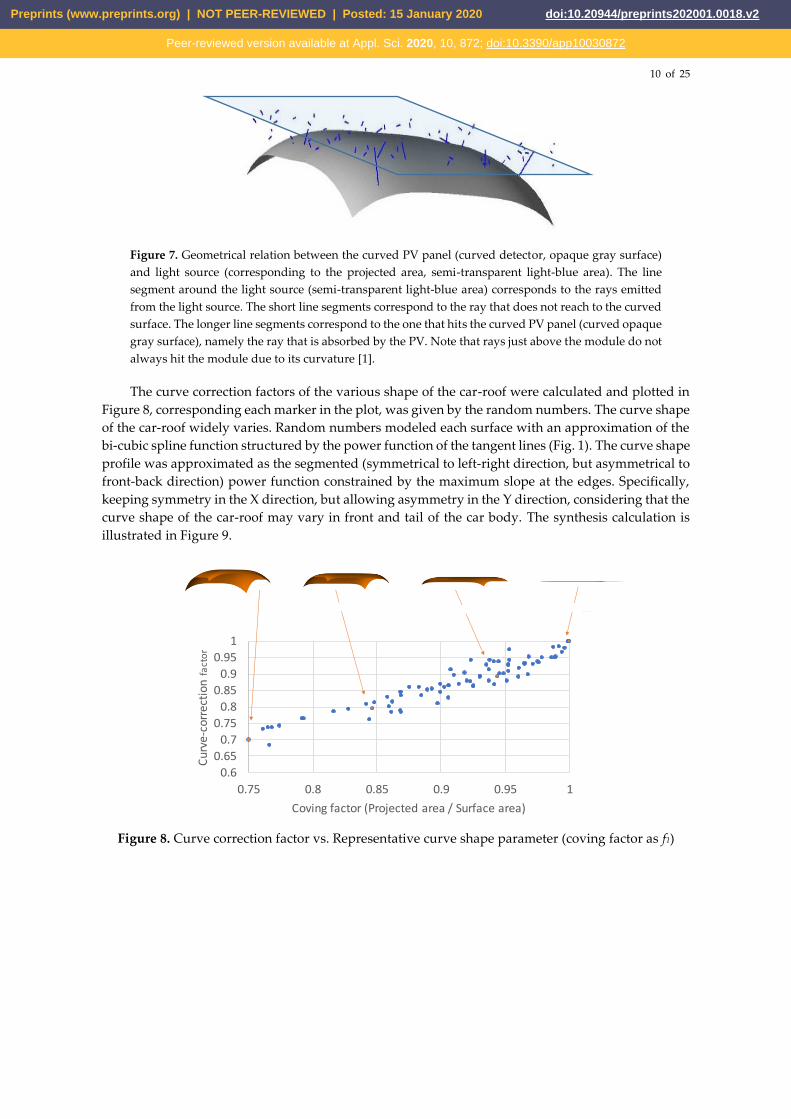
Figure 7. Geometrical relation between the curved PV panel (curved detector, opaque gray surface)
and light source (corresponding to the projected area, semi-transparent light-blue area). The line
segment around the light source (semi-transparent light-blue area) corresponds to the rays emitted
from the light source. The short line segments correspond to the ray that does not reach to the curved
surface. The longer line segments correspond to the one that hits the curved PV panel (curved opaque
gray surface), namely the ray that is absorbed by the PV. Note that rays just above the module do not
always hit the module due to its curvature [1].
The curve correction factors of the various shape of the car-roof were calculated and plotted in
Figure 8, corresponding each marker in the plot, was given by the random numbers. The curve shape
of the car-roof widely varies. Random numbers modeled each surface with an approximation of the
bi-cubic spline function structured by the power function of the tangent lines (Fig. 1). The curve shape
profile was approximated as the segmented (symmetrical to left-right direction, but asymmetrical to
front-back direction) power function constrained by the maximum slope at the edges. Specifically,
keeping symmetry in the X direction, but allowing asymmetry in the Y direction, considering that the
curve shape of the car-roof may vary in front and tail of the car body. The synthesis calculation is
illustrated in Figure 9.
Figure 8. Curve correction factor vs. Representative curve shape parameter (coving factor as f1)
0.6
0.65
0.7
0.75
0.8
0.85
0.9
0.95
1
0.75 0.8 0.85 0.9 0.95 1
Cur
ve-c
orre
ctio
nfa
cto
r
Coving factor (Projected area / Surface area)
Preprints (www.preprints.org) | NOT PEER-REVIEWED | Posted: 15 January 2020 doi:10.20944/preprints202001.0018.v2
Peer-reviewed version available at Appl. Sci. 2020, 10, 872; doi:10.3390/app10030872
11 of 25
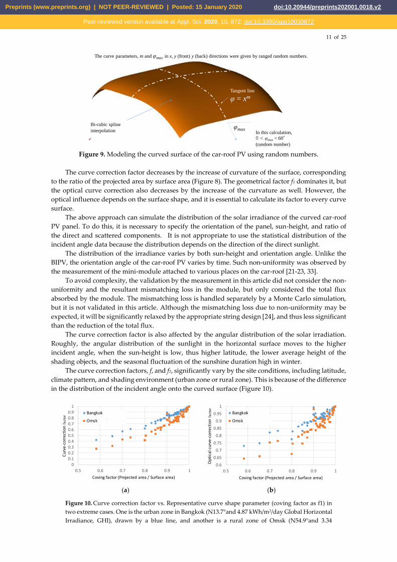
Figure 9. Modeling the curved surface of the car-roof PV using random numbers.
The curve correction factor decreases by the increase of curvature of the surface, corresponding
to the ratio of the projected area by surface area (Figure 8). The geometrical factor f1 dominates it, but
the optical curve correction also decreases by the increase of the curvature as well. However, the
optical influence depends on the surface shape, and it is essential to calculate its factor to every curve
surface.
The above approach can simulate the distribution of the solar irradiance of the curved car-roof
PV panel. To do this, it is necessary to specify the orientation of the panel, sun-height, and ratio of
the direct and scattered components. It is not appropriate to use the statistical distribution of the
incident angle data because the distribution depends on the direction of the direct sunlight.
The distribution of the irradiance varies by both sun-height and orientation angle. Unlike the
BIPV, the orientation angle of the car-roof PV varies by time. Such non-uniformity was observed by
the measurement of the mini-module attached to various places on the car-roof [21-23, 33].
To avoid complexity, the validation by the measurement in this article did not consider the non-
uniformity and the resultant mismatching loss in the module, but only considered the total flux
absorbed by the module. The mismatching loss is handled separately by a Monte Carlo simulation,
but it is not validated in this article. Although the mismatching loss due to non-uniformity may be
expected, it will be significantly relaxed by the appropriate string design [24], and thus less significant
than the reduction of the total flux.
The curve correction factor is also affected by the angular distribution of the solar irradiation.
Roughly, the angular distribution of the sunlight in the horizontal surface moves to the higher
incident angle, when the sun-height is low, thus higher latitude, the lower average height of the
shading objects, and the seasonal fluctuation of the sunshine duration high in winter.
The curve correction factors, f, and f2, significantly vary by the site conditions, including latitude,
climate pattern, and shading environment (urban zone or rural zone). This is because of the difference
in the distribution of the incident angle onto the curved surface (Figure 10).
(a) (b)
Figure 10. Curve correction factor vs. Representative curve shape parameter (coving factor as f1) in
two extreme cases. One is the urban zone in Bangkok (N13.7°and 4.87 kWh/m2/day Global Horizontal
Irradiance, GHI), drawn by a blue line, and another is a rural zone of Omsk (N54.9°and 3.34
φmax
Tangent line
φ = xm
Bi-cubic spline
interpolation
The curve parameters, m and φmax in x, y (front) y (back) directions were given by ranged random numbers.
In this calculation,
0 < φmax < 60°
(random number)
Generalization of the parametric surface profile for anal-ysis of performance of the curved PV, including unde-velopable curved surface
0
0.1
0.2
0.3
0.4
0.5
0.6
0.7
0.8
0.9
1
0.5 0.6 0.7 0.8 0.9 1
Cu
rve
-co
rrec
tio
nfa
cto
r
Coving factor (Projected area / Surface area)
Bangkok urban zone
Omsk rural zone
0.6
0.65
0.7
0.75
0.8
0.85
0.9
0.95
1
0.5 0.6 0.7 0.8 0.9 1
Op
tica
l cu
rve-
corr
ecti
on
fact
or
Coving factor (Projected area / Surface area)
Bangkok urban zone
Omsk rural zone
Preprints (www.preprints.org) | NOT PEER-REVIEWED | Posted: 15 January 2020 doi:10.20944/preprints202001.0018.v2
Peer-reviewed version available at Appl. Sci. 2020, 10, 872; doi:10.3390/app10030872
12 of 25
kWh/m2/day GHI) drawn in orange line. : (a) curve-correction factor f; (b) optical curve correction
factor f2.
2.6. Partial and dynamic shading modell
The shading influence is complicated and varies by the position and the relative orientation (to
the sun position) of the panel. In the case of the car-roof PV, the position (orientation) of the panel
cannot be predicted. One practical approach is to rely on the probability model, supposing that the
distribution and height of the shading objects are randomly distributed by some statistical model and
the orientation of the car is independent and random as well.
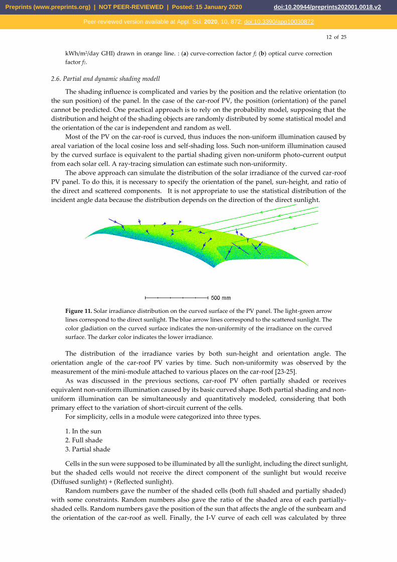
Most of the PV on the car-roof is curved, thus induces the non-uniform illumination caused by
areal variation of the local cosine loss and self-shading loss. Such non-uniform illumination caused
by the curved surface is equivalent to the partial shading given non-uniform photo-current output
from each solar cell. A ray-tracing simulation can estimate such non-uniformity.
The above approach can simulate the distribution of the solar irradiance of the curved car-roof
PV panel. To do this, it is necessary to specify the orientation of the panel, sun-height, and ratio of
the direct and scattered components. It is not appropriate to use the statistical distribution of the
incident angle data because the distribution depends on the direction of the direct sunlight.
Figure 11. Solar irradiance distribution on the curved surface of the PV panel. The light-green arrow
lines correspond to the direct sunlight. The blue arrow lines correspond to the scattered sunlight. The
color gladiation on the curved surface indicates the non-uniformity of the irradiance on the curved
surface. The darker color indicates the lower irradiance.
The distribution of the irradiance varies by both sun-height and orientation angle. The
orientation angle of the car-roof PV varies by time. Such non-uniformity was observed by the
measurement of the mini-module attached to various places on the car-roof [23-25].
As was discussed in the previous sections, car-roof PV often partially shaded or receives
equivalent non-uniform illumination caused by its basic curved shape. Both partial shading and non-
uniform illumination can be simultaneously and quantitatively modeled, considering that both
primary effect to the variation of short-circuit current of the cells.
For simplicity, cells in a module were categorized into three types.
1. In the sun
2. Full shade
3. Partial shade
Cells in the sun were supposed to be illuminated by all the sunlight, including the direct sunlight,
but the shaded cells would not receive the direct component of the sunlight but would receive
(Diffused sunlight) + (Reflected sunlight).
Random numbers gave the number of the shaded cells (both full shaded and partially shaded)
with some constraints. Random numbers also gave the ratio of the shaded area of each partially-
shaded cells. Random numbers gave the position of the sun that affects the angle of the sunbeam and
the orientation of the car-roof as well. Finally, the I-V curve of each cell was calculated by three
Preprints (www.preprints.org) | NOT PEER-REVIEWED | Posted: 15 January 2020 doi:10.20944/preprints202001.0018.v2
Peer-reviewed version available at Appl. Sci. 2020, 10, 872; doi:10.3390/app10030872

13 of 25
randomly distributed three parameters (normal distribution). The property of the probability
variables used for the Monte Carlo simulation is summarized in Table 1. The irradiance and climate
conditions corresponding to the above parameters were looked into in the database of METPV-11
and METPV-Asia [43-45]. Given those probability parameters, I-V curves of entire cells in the array
affected different illumination conditions, and variations of characteristics were calculated, and the
maximum power point was calculated for taking the simulated power output affected by the partial
shading.
Table 1. Summary of random variables used to the Monte Carlo simulation.
Section Distribution Type Range
Date (Day number)1 Uniform distribution Integer 0 – 364 (day)
Time1 Uniform distribution Integer 0 – 23 (hour)
Number of cells partially shaded2 Uniform distribution Integer 0 – (Number of cells in the string)
Number of cells fully shaded2 Uniform distribution Integer 0 – (Number of cells in the string)
Shading ratio of each partially-shaded cell3 Uniform distribution Real 0 - 1
Car orientation4 Uniform distribution Real 0°- 360°
Isc of each cell Normal distribution Real --
Voc of each cell Normal distribution Real --
Diode ideality5 Normal distribution Real Greater than 1
1 Repeat throwing a dice until the horizontal global sunlight given by the database is more than 1 Wh/m2 to
avoid the inclusion of the trial in the night time. The bissextile day is removed. 2 Random numbers are given to each string. The number of partial and full shaded cells must be less than the
number in the strings. 3 The ratio of the partial shading (0 to 1)
4 Assuming that the car always parks or runs on the horizontal plane. 5 Representing the shape of the I-V curve
It is important to note that the probability modeling of the partial shading, corresponding to the
forth to sixth rows of Table 2, is the key to the simulation. For minimizing the evil influence of the
partial shading, the PV and car manufacturers try to place the series strings as close to the shape of
the partial shading or non-uniform illumination pattern caused by the curvature of the car-body as
possible, In a way, the distribution of the shaded cells are not uniformly distributed but leaves some
distribution pattern. To mimic this situation, the random model was made by three steps (see 4th to
sixth rows of Table 1). Specifically, the number of the shaded cells in each string was allocated using
Equation (21), and the short-circuit current from each cell impacted by shading was given in equation
(2). Note both equation (1) and equation (2) contains Boolean algebra. It is also important to note that
the vector and matrix data that were generated by the above calculation and contains the information
of the shaded ratio of each cell in the module is only used as the circuit calculation of the module by
series-parallel connection with bypass diodes. Therefore, in the downstream calculation step, the
position of the shaded cell is not referred, but they may be redistributed in the series connection by
order of the shaded ratio.
Preprints (www.preprints.org) | NOT PEER-REVIEWED | Posted: 15 January 2020 doi:10.20944/preprints202001.0018.v2
Peer-reviewed version available at Appl. Sci. 2020, 10, 872; doi:10.3390/app10030872

14 of 25
𝐒𝐅(𝑛, 𝑁𝑠𝑡𝑟𝑖𝑛𝑔𝑠) ∶=
‖
‖
‖
‖
‖
if 𝑁𝑠𝑡𝑟𝑖𝑛𝑔𝑠 < 2
‖𝐮0 ← 𝐟𝐥𝐨𝐨𝐫(𝐫𝐧𝐝(𝑛))‖
else
‖
‖
‖
‖
𝐯0 ← 𝐟𝐥𝐨𝐨𝐫(𝐫𝐧𝐝(𝑛))
for 𝑖 ∈ 1 … 𝑁𝑠𝑡𝑟𝑖𝑛𝑔𝑠 − 1
‖‖
𝑠𝑢𝑚 ← ∑ 𝐯𝑗−1𝑖𝑗=1
𝐯𝑖 ← 𝐢𝐟(𝑛 − 𝑠𝑢𝑚 > 0, 𝐟𝐥𝐨𝐨𝐫(𝐫𝐧𝐝(𝑛 − 𝑠𝑢𝑚)), 0)
𝐯 ← 𝐬𝐭𝐚𝐜𝐤(𝐯, 𝐯𝑖)
‖‖
𝐮 ← 𝐬𝐮𝐛𝐦𝐚𝐭𝐫𝐢𝐱(𝐯, 0, 𝑁𝑠𝑡𝑟𝑖𝑛𝑔𝑠 − 1,0,0)
𝐮0 ← 𝑛 − ∑ 𝐮𝑗𝑁𝑠𝑡𝑟𝑖𝑛𝑔𝑠−1𝑗=1
𝐮
‖
‖
‖
‖
‖
‖
‖
‖
‖
(21)
𝐈𝐫𝑖,𝑗=
𝑆𝑇𝐼+((𝑗<𝐒𝐜𝐧𝑖)+𝐢𝐟((𝐒𝐜𝐧𝑖≤𝑗<𝐒𝐧𝐩𝑖+𝐒𝐜𝐧𝑖)∧𝐒𝐧𝐩𝑖>0,𝐫𝐮𝐧𝐢𝐟(𝐒𝐧𝐩𝑖,0,1)𝑗−𝐒𝐜𝐧𝑖,0))∙𝐷𝑇𝐼
𝑇𝐼𝑆(22)
where, SF(n, Nstrings) is a function that generates a vector containing the number of shaded cells in
each string. n is a scalar parameter of the number of the cells in a string. Nstrings is a scalar parameter
of the number of the strings in a module. floor(z) is a function that returns the greatest integer ≤ z.
rnd(x) is a function that returns a uniformly distributed random number between 0 and x. if(cond, x,
y) is a function returns x if cond is true (nonzero), y otherwise. stack(A , B, C, ...) is a function that
returns an array formed by placing A, B, C, ... top to bottom. submatrix(A, ir, jr, ic, jc) is a function
that returns the matrix consisting of rows ir through jr and columns ic through jc of array A. Ir in
Equation (22) is an array that contains solar irradiance of each cell in the module affected by partial
shadings. STI is a scalar parameter of the diffused sunlight onto the module plane. Scn is a vector
that contains a number of the unshaded cells in each string in the module. Snp is a vector that contains
a number of partially shaded cells in strings. runif(m, a, b) is a function that returns a vector of m
random numbers having the uniform distribution, and m is a scalar of real values, a ≤ m ≤ b. To allow
integration and other operations over this argument, values outside of the stated range are allowed,
but they produce a 0 result. a and b are real numbers, a < b. DTI is a scalar parameter of the direct
sunlight onto the module plane. TIS is a scalar parameter of the total sunlight onto the module plane.
3. Results
In this article, we evaluated the annual irradiance incident on the car using five pyranometers
located in five orthogonal directions. We also presented the seasonal variation of the angular
distribution of the leading solar beam and the annually angular distribution model on car-roof.
3.1. 3-D measurement by multiple pyranometer array
The measurement system consisted of five pyranometers mounted on the car roof, along with a
GPS, and thus, could be moved on the road. The pyranometer axes Qx+, Qx-, Qy+, Qy-, and Qz were
defined, as shown in Figure 1and 12. One pyranometer was placed horizontally on the car roof (Qz),
and four pyranometers were placed vertically facing each side of the car (Qx+, Qx-, Qy+, Qy-). The global
irradiance onto the car roof (Iz) was measured using a pyranometer Qz. The global irradiance onto the
side of the car (Ix+, Ix-, Iy+, Iy-) was measured using pyranometers Qx+, Qx-, Qy+, Qy-. The direction of the
moving car was equal to that of Qy+. An ambient temperature meter (Pt 100 temperature sensor) was
also placed on the car roof. The GPS was incorporated into the data logger, and data was recorded in
1 s intervals. The total number of hours of sun radiation (more than 10 W/m2 in Iz) received over the
year was 3374 h, while the number of hours the car was running was approximately 6% of this.
To acquire a dataset for comparison, a conventional static irradiance measurement system with
a pyrheliometer, a tracking pyranometer mounted onto a sun tracker, a horizontal pyranometer, and
two vertical pyranometers facing eastward and westward was installed at the University of Miyazaki,
Preprints (www.preprints.org) | NOT PEER-REVIEWED | Posted: 15 January 2020 doi:10.20944/preprints202001.0018.v2
Peer-reviewed version available at Appl. Sci. 2020, 10, 872; doi:10.3390/app10030872

15 of 25
Japan (31°49’N, 131°24’E). The elevation angle and azimuth angle of the sun position were calculated
based on the conventional method, including the day angle, declination angle, time equation, hour
angle, latitude, and longitude.
Figure 12. Measurement system on the car using five pyranometers on the orthogonal axis.
3.2 Measurement example of the solar irradiance on the car-roof and car-side
The city of Miyazaki, Japan, is one of the capitals of local government in Japan (Miyazaki
prefecture) with approximately 200 thousand population. Thus, this area contains an urban zone, a
residential zone, and a rural zone. In a way, it may be a representative zone in the solar environment
(shading frequency and shading height). We did not constrain the driving course of the one-year
monitoring of the solar irradiance on the car, but the most frequent driving course of this car is shown
in Figure 13 since it was used for commuting between the University of Miyazaki and driver’s
residence.
Figure 13. Most-frequent driving course of the dynamic solar irradiance measurement in the car.
The typical monitored result in the route in Figure 13 is shown in Figure 14 (clear sky day) with
comparison to the Global Horizontal Irradiance (GHI) of fixed pyranometers (mounted on a roof of
one of the buildings of the University of Miyazaki).
In the region of the open-air section, the solar irradiance on the car-roof was almost identical to
the GHI by the fixed pyranometers. However, that of other areas had frequent dips in the irradiance
on the car. The timestamp and position data taken by GPS confirmed that these were because of the
shading effects by buildings and mountains. The car-roof irradiance often exceeded GHI. It was also
confirmed because of the reflectance of the buildings.
High-rise section
Urban section
Open-air section
Miyazaki Station
University of Miyazaki
10 km
Preprints (www.preprints.org) | NOT PEER-REVIEWED | Posted: 15 January 2020 doi:10.20944/preprints202001.0018.v2
Peer-reviewed version available at Appl. Sci. 2020, 10, 872; doi:10.3390/app10030872

16 of 25
Figure 14. Monitored the result of the solar irradiance on the car-roof and car-sides in the driving
route in Figure 13.
3.3 Validation of the solar irradiation model around the car (intensity)
The above model was compared with the one-year observation result of the solar irradiance to
the vehicle, including seasonal (monthly) fluctuation. After fitting to the measurement irradiance
dataset, the fitted average shading height was 18.7° in the direction along the road (local axis) and
12.3°in the direction orthogonal to the road (local axis), and 15.5° as the average. The averaged
shading height after data fit was 15.5°, and it was very closed from the value of rough physical
measurement (15° on average). The average reflectance from the road was also fit to the measured
data and was obtained as 0.088, also reasonable value for aged asphalt (typical value is 0.07). The
comparison to the measured irradiance and modeled irradiance were compared in Table 2.
Table 2. Comparison of model and measurement (relative to GHI) by one-year monitoring of a
passenger’s car
Measured Model by rough physical
measurement
Modeled by parameter fit
(average height of shading objects and
reflectance of the road)1
Car-roof 0.925 0.929 0.925
Car-side (x-direction) 0.395 0.412
0.395
Car-side (y-direction) 0.435 0.435
1 The degree of freedom and the number of fit parameters are the same (= 3).
The validation was also done by a one-month integration (seasonal fluctuation). The model met
the modeled values in every month (Figure 14). The trend of the residual errors could be explained
by the difference in climate from the regular year (for example, cloudy in summer).
(a) (b)
Figure 14. Monthly-based comparison between the measured solar irradiance around the car (bar-
chart) and modeled (typical year from the METPV-11 solar database) solar irradiance on the car (line-
chart): (a) car-roof irradiance; (b) car-side irradiance.
High-rise sectionOpen-air section Urban section
0
0.2
0.4
0.6
0.8
1
Jan Feb Mar Apr May Jun Jul Aug Sep Oct Nov Dec
Car
-ro
of
/ G
HI
Measured Model
0
0.2
0.4
0.6
0.8
1
Jan Feb Mar Apr May Jun Jul Aug Sep Oct Nov Dec
Car
-sid
e /
GH
I
Measured Model
Preprints (www.preprints.org) | NOT PEER-REVIEWED | Posted: 15 January 2020 doi:10.20944/preprints202001.0018.v2
Peer-reviewed version available at Appl. Sci. 2020, 10, 872; doi:10.3390/app10030872

17 of 25
(a) (b)
Figure 15. Daily-based comparison between the measured solar irradiance around the car (blue dots)
and modeled (typical year from the METPV-11 solar database) solar irradiance on the car (orange
dots): (a) car-roof irradiance; (b) car-side irradiance.
The same comparison was made in daily-base (Figure 15). Since every day’s climate was not
always identical to the one in the solar database, there were significant errors in the time-series trend.
However, the range of the distribution in the modeled irradiance was almost the same as the
measured irradiance.
3.4 Validation of the solar irradiation model around the car (Angle)
After validation of the irradiance model affected by the surrounding shading objects, the
histogram of the car irradiance was counted using the one-year irradiation model. The results of
annually integrated angular distribution were shown in Figure 16. For examining the seasonal trend,
the weighted histograms of the angular distribution of the leading solar beam in each month were
plotted in Figure 17. The residual error of the model was observed in more than 30° of incident angle
or winter season (corresponding low sun-height and high incident angle). It is possible because the
model of the shading height distribution was too simplified. However, the overall trend met the
measured one, and the angular model can be used for a rough estimation of the solar irradiance
environment around the car-body.
Figure 16. Annually-integrated angular distribution (weighted histogram of the leading solar beam).
0.8
0.85
0.9
0.95
1
1.05
0 2000 4000 6000 8000 10000
Ca
r-ro
of
irra
ida
nce
(to
p)
pe
r G
HI
Global horizontal irradiance per day (Wh/m2)
Measured
Model
0
0.1
0.2
0.3
0.4
0.5
0.6
0.7
0 2000 4000 6000 8000 10000
Car
-ro
of
irra
ida
nce
(sid
e)
pe
r G
HI
Global horizontal irradiance per day (Wh/m2)
Measured
Model
0%
2%
4%
6%
8%
10%
0 15 30 45 60 75 90
Wei
ghte
d p
erce
nta
ge
Incident angle (deg)
ModelMeasurement
Preprints (www.preprints.org) | NOT PEER-REVIEWED | Posted: 15 January 2020 doi:10.20944/preprints202001.0018.v2
Peer-reviewed version available at Appl. Sci. 2020, 10, 872; doi:10.3390/app10030872

18 of 25
Figure 16. Monthly-integrated angular distribution (weighted histogram of the leading solar beam).
Jan. Feb.
Mar Apr.
May Jun.
Jul. Aug.
Sep. Oct.
Nov. Dec.
0%
5%
10%
15%
20%
25%
30%
0 15 30 45 60 75 90
Wei
ghte
d p
erce
nta
ge
Incident angle (deg)
ModelMeasurement
0%
5%
10%
15%
20%
25%
30%
0 15 30 45 60 75 90
Wei
ghte
d p
erce
nta
ge
Incident angle (deg)
ModelMeasurement
0%
5%
10%
15%
20%
25%
30%
0 15 30 45 60 75 90
Wei
ghte
d p
erce
nta
ge
Incident angle (deg)
ModelMeasurement
0%
5%
10%
15%
20%
25%
30%
0 15 30 45 60 75 90
Wei
ghte
d p
erce
nta
ge
Incident angle (deg)
ModelMeasurement
0%
5%
10%
15%
20%
25%
30%
0 15 30 45 60 75 90
Wei
ghte
d p
erce
nta
ge
Incident angle (deg)
ModelMeasurement
0%
5%
10%
15%
20%
25%
30%
0 15 30 45 60 75 90
Wei
ghte
d p
erce
nta
ge
Incident angle (deg)
ModelMeasurement
0%
5%
10%
15%
20%
25%
30%
0 15 30 45 60 75 90
We
igh
ted
pe
rce
nta
ge
Incident angle (deg)
Model
Measurement
0%
5%
10%
15%
20%
25%
30%
0 15 30 45 60 75 90
Wei
ghte
d p
erce
nta
ge
Incident angle (deg)
ModelMeasurement
0%
5%
10%
15%
20%
25%
30%
0 15 30 45 60 75 90
We
igh
ted
pe
rce
nta
ge
Incident angle (deg)
ModelMeasurement
0%
5%
10%
15%
20%
25%
30%
0 15 30 45 60 75 90
We
igh
ted
pe
rce
nta
ge
Incident angle (deg)
ModelMeasurement
0%
5%
10%
15%
20%
25%
30%
0 15 30 45 60 75 90
Wei
ghte
d p
erce
nta
ge
Incident angle (deg)
ModelMeasurement
0%
5%
10%
15%
20%
25%
30%
0 15 30 45 60 75 90
Wei
ghte
d p
erce
nta
ge
Incident angle (deg)
ModelMeasurement
Preprints (www.preprints.org) | NOT PEER-REVIEWED | Posted: 15 January 2020 doi:10.20944/preprints202001.0018.v2
Peer-reviewed version available at Appl. Sci. 2020, 10, 872; doi:10.3390/app10030872

19 of 25
4. Discussion.
4.1. Simplified rating method of VIPV considering 3-dimensional solar irradiance
The standard rating measurement for PV is done by a single measurement in the normal
illumination. However, that of VIPV is not sufficient because it uses three-dimensional solar
irradiance by curved module and three-dimensional installation (frequently, the PV module on the
car-side is added).
The ratio of solar resource measurement is useful for a quick rating of the VIPV system on the
car by three-dimensional measurement. A possible step is as follows:
1. Measure the PV performance in 5 directions (see Figure 2).
2. The rating of the total performance in the specific area can be weighted by the normalized
solar resources using Equation (23) and the values in Table 2, namely,
𝑃 = 𝑎𝑃𝑧 + 𝑏(𝑃𝑥+ + 𝑃𝑥−) + 𝑐(𝑃𝑦+ + 𝑃𝑦−) (23)
where, P is the rated power output. Pz is the measured power output by the illumination on the car-
roof. Px+, Px-, Py+, and Py1 are the measured power outputs by the illumination on the car-sides in the
direction defined in Figure 1. a, b, and c are weighting coefficient given by Table 2. Note that the
coefficients a, b, and c in our measurement in Miyazaki, Japan is 0.925, 0.395, and 0.435. The Equation
(21) gives a total energy output of the entire PV system on the vehicle considering 3-D solar irradiance
around the vehicle comparable to GHI.
4.2. Estimation of the practical solar resource to VIPV in other regions
Assuming that the density and height distribution of the shading objects are the same to that of
Miyazaki, Japan, namely the average shading height is about 15.5°, it may be possible to anticipate
the energy yield of the VIPV in various area in the world, that is useful to anticipate the merits of the
introduction of the solar-driven vehicles.
Figure 17 indicates the map of the practical solar resource on the car-roof normalized to the GHI,
affected by climate conditions. They were calculated using a model in section 2.2 and 2.5, using
METPV-ASIA solar irradiance database. Due to the shading impact and curved surface, the practical
solar resource for the car-roof is less than the typical installation. The rough value maybe 3/4 of the
GHI.
Generally speaking, both the shading impact and curve impact increases with the decrease of
the sun-height, namely, increasing the latitude. However, both curve-correction factor and effective
solar resource to the car-roof normalized to GHI (including the loss by the curved surface), do not
show a strong correlation to latitude (thus sun-height), unlike other typical solar resource parameters,
it is affected by local meteorological conditions. Also, note that both the curve-correction factor and
the effective solar resource relative to GHI are strongly affected by the distribution (both special and
height) of shading objects.
Preprints (www.preprints.org) | NOT PEER-REVIEWED | Posted: 15 January 2020 doi:10.20944/preprints202001.0018.v2
Peer-reviewed version available at Appl. Sci. 2020, 10, 872; doi:10.3390/app10030872

20 of 25
(a) (b)
(c) (d)
Figure 17. Map of the effective solar irradiance for the car-roof: (a) Curve-correction factor in typical
car-roof; (b) Effective solar resource to the car-roof normalized to GHI, including the loss by the
curved surface; (c) Correlations between latitude (related to the sun height) and the curve correction
factor; Correlations between latitude (related to sun height) and the effective solar resource to the car-
roof normalized to GHI, including the loss by the curved surface
4.3. Partial shading issue
Since calculated power and related loss were affected by probability variables, the calculated
result was not a single number but showed distribution. Fig. 8 shows an example of the distribution
of the normalized efficiency of several array designs of the car-roof PV, affected by the mismatching
loss result from partial shading. The ratio of the power output of the partially shaded module is less
than the ratio of the area in the sun. The reduction ratio corresponds to the mismatching loss. The
loss factor is a function of the number of strings, curvature of the car-roof, and latitude.
0.82
0.83
0.84
0.85
0.86
0.87
0.88
0.89
0 15 30 45 60
Cu
rve
-co
rrec
tio
n fa
cto
r
Latitude (deg)
72%
74%
76%
78%
80%
82%
84%
0 15 30 45 60Sola
r re
sou
rce
re
lati
ve t
o G
HI
Latitude (deg)
Preprints (www.preprints.org) | NOT PEER-REVIEWED | Posted: 15 January 2020 doi:10.20944/preprints202001.0018.v2
Peer-reviewed version available at Appl. Sci. 2020, 10, 872; doi:10.3390/app10030872

21 of 25
Figure 18. Distribution of the normalized efficiency of some design of the car-roof PV affected by
synthesized partial shading given by the Monte Carlo simulation. Note 1/6 or more cut is
recommended for suppressing partial-shading loss to < 10%.
4.4. Limitation of the model
First, the model discussed in this article relied on the random number and assumed that every
parameter affecting the solar resource on the car-roof and car-side is distributed by a simple rule, for
example, ranged uniform distribution. It may be meaningful to the averaged or integrated energy
yield, but cannot be applied to the power prediction in specific driving point and direction, specific
climate as well as specific surrounding conditions. The given distributions may not be equal to the
real situation that varies every position and every time. In this sense, it is to be applied to annual or
other long-term integration like annual energy yield.
Distribution of the shading objects (both spacial distribution and height distribution) is essential
to the model. Our model is based on a linear trend (Figure 2) but was too simplified to the shading
in the high-rise section in Figure 13, where the trend of Figure 2 may become trapezoid or other
complicated shapes. Namely, the energy yield in the urban area may give optimistically-biased value.
For the moment, the impact by the partial shading has not been considered yet. We only
estimated the impact of using a Monte Carlo simulation. Depending on the string configuration or
the power-conditioner connected to the car-mounted module, the output power may drop by the
mismatching loss that was not anticipated to the model.
4.5 Feasibility of the VIPV based on our measurement and modeling
Compared with the past report by Toyota Motors [2] and NEDO [3] that did not consider the
shading effect by surrounding objects and loss by the curved surface, our research gave a more
realistic solar resource on the car-roof and car-side. These two reports gave an overestimation of the
energy yield expectation. The rough number suggested by this research is around 3/4 using highly
curved PV modules on the car-roof and shading effects (taken by the capital of the local government
in Japan).
As it is measured and modeled in this study, the energy yield of VIPV is undoubtedly less than
that of the PV power plant that is constructed maximizing the energy yield by a given amount of the
solar panels. However, considering that the related soft-cost and other balance of system cost
(construction, structure, connecting to the grid, distribution, and the cost of the constructing and
operation of the EV charging station) that are to be eventually shared by car-owners or car-
manufacturers, VIPV will be attractive option both in cost and user-friendliness.
4.6 Future works
1/2 cut, 4 strings
1/8 cut, 16 strings
1/4 cut, 8 strings
Preprints (www.preprints.org) | NOT PEER-REVIEWED | Posted: 15 January 2020 doi:10.20944/preprints202001.0018.v2
Peer-reviewed version available at Appl. Sci. 2020, 10, 872; doi:10.3390/app10030872

22 of 25
For improvement of the energy yield prediction of VIPV, the following works are to be done.
1. Improvement of the shading model. The current model is useful but too simplified,
especially in the urban area. Note that more than 45° of the average shading height is not
allowed, because the maximum height becomes more than 90°. Even in the area of Miyazaki,
the average height of 15.5° means that the maximum height should be 31°. However, there
were many buildings of more than 31°. Possibly, we need to develop a curved trend, namely
the two parameters model.
2. Modeling of partial shading validated to the measured data. To do this, we need to start
monitoring the partial shading on the car-roof and car-body.
3. Validation of energy yield using the real curved PV module.
4. Validation of the shading model by several areas with different shading height and shading
density.
5. Development of the spectrum model for predicting energy yield by multi-junction solar cells
on the car-roof and car-body.
5. Conclusions
Increasing the concern of the greenhouse gas emissions in the transportation sectors, the fuel,
and engine of the car is required to consider the total emission of CO2 by a well-to-wheel basis. The
typical approach is an electric vehicle (EV) charged by the electricity generated by renewable energy
like solar power. However, this approach relies on the infrastructure of the distribution of the clean
electricity (PV power station installation, grid construction and connection, distribution of the clean
electricity, and installation and operation of the EV charging station). It is much more convenient
than the car collects solar energy and runs by it (or at least extending the range of mileage supported
by its PV modules to reduce the frequency of charging).
The solar-powered vehicles are now seriously discussed, and we had several feasibility reports
[2-3]. In principle, it is feasible by the improvement of both PV and car technologies to run a majority
of electric vehicles on solar energy. However, as it is often the case of the early feasibility study, it is
not supported by the real solar resources of the car running in the real environment. The motivation
for our study is to know the real and active solar energy for the car through both modeling and
measurement.
For modeling, we developed a simple shading model using a uniformly distributed (density and
height) shading objects and random driving orientation using a simple combination of the collimated
direct sunlight, uniform diffused sunlight, and reflection by road and shading objects. For the
validation of the model, we used an array of pyranometers mounted on the car in 5 axes and
monitored the solar resource around the car for one year. The model was validated in x, y, and z-
direction local to the car as well as the angular distribution of the main beam of the solar irradiance
on the car-roof.
Additionally, we developed by the correction method of the curved surface of the car-roof and
car-body. Commonly, the car-roof and car-body is curved, and the car-manufacturers wanted that
the PV panels are also curved fit to the car-body. The measurement (indoor testing) and performance
(outdoor operation) in the standard PV panel was established by the fact that the PV panel always
has a flat surface. We had to construct both the testing method and operation model from the
beginning considering the three-dimensional density of the photon energy absorbance. Our solution
is to introduce a curve-correction factor with keeping compatibility with the current testing
equipment and standards. The curve-correction factor can be calculated by the ray-tracing calculation,
once both the curve profile (possibly by CAD file) and angular distribution of the solar irradiance
(also given by those mentioned above by the new solar resource model on the car-body).
Another crucial factor that affects energy yield from the VIPV is the mismatching loss either by
the partial shading and non-uniform distribution by the curved surface. Currently, we developed a
Monte Carlo simulation assuming that random numbers give the non-uniformity and ratio of the
partial shading.
Here is a summary of the conclusion in technical issues;
Preprints (www.preprints.org) | NOT PEER-REVIEWED | Posted: 15 January 2020 doi:10.20944/preprints202001.0018.v2
Peer-reviewed version available at Appl. Sci. 2020, 10, 872; doi:10.3390/app10030872

23 of 25
1. A simple shading model to VIPV was developed and validated by one-year monitoring on
the solar irradiation on the car-roof and car-body in 5 axes.
2. The curve-correction model of the curved surface of VIPV was developed.
3. Mismatching model using Monte Carlo simulation was developed to analysis on the partial
shading of VIPV.
Author Contributions: Conceptualization, K.A.; methodology, Y.O.; software, K.A.; validation, Y.O.;
investigation, Y.O.; data curation, Y.O.; writing—original draft preparation, K.A.; writing—review and editing,
Y.O.; visualization, K.A., and Y.O.; supervision, Y.O.; project administration, M.Y.; funding acquisition, M.Y.
Funding: Part of this research was funded by the New Energy and Industrial Technology Development
Organization (NEDO) under the Ministry of Economy, Trade, and Industry (METI), Japan.
Acknowledgments: The modeling of VIPV was first discussed in the international web meetings (76 scientists
and engineers are registered) for the standardization of the car-roof PV, starting discussions in December 2017.
Part of this research was funded by NEDO, Japan. The standardization activities was supported by JEMA, Japan.
Conflicts of Interest: The authors declare that there is no conflict of interest.
References
1. Araki, K.; Ji, L.; Kelly, G.; Yamaguchi, M. To Do List for Research and Development and International
Standardization to Achieve the Goal of Running a Majority of Electric Vehicles on Solar Energy. Coatings
2018, 8, 251.
2. Masuda, T.; Araki, K.; Okumura; K.; Urabe, S.; Kudo, Y.; Kimura, K.; Nakado, T.; Sato, A.; Yamaguchi, M.;
Static concentrator photovoltaics for automotive applications. Solar Energy 2017, 146, 523-531.
3. NEDO, Interim Report of the Exploratory Committee on the Automobile Using Photovoltaic System.
4. Masuda, T.; Araki, K.; Okumura, K.; Urabe, S.; Kudo, Y.; Kimura, K.; Nakado, T.; Sato, A.; Yamaguchi, M.
Next environment-friendly cars: Application of solar power as automobile energy source. In Proceedings
of the 2016 IEEE 43rd Photovoltaic Specialists Conference (PVSC), Portland, OR, USA, 5–10 June 2016; pp.
0580–0584.
5. Araki, K.; Sato, D.; Masuda, T.; Lee, KH.; Yamada, N.; Yamaguchi, M. Why and how does car-roof PV create
50 GW/year of new installations? Also, why is a static CPV suitable to this application?. InAIP Conference
Proceedings 2019 Aug 26 (Vol. 2149, No. 1, p. 050003). AIP Publishing.
6. Stutzmann, M. Role of mechanical stress in the light‐induced degradation of hydrogenated amorphous
silicon. Applied Physics Letters, 1985, 47(1), 21-23.
7. Moeini, I.; Ahmadpour, M.; Mosavi, A.; Alharbi, N.; Gorji, N. E. Modeling the time-dependent
characteristics of perovskite solar cells. Solar Energy, 2018, 170, 969-973.
8. Lindroos, J.; Savin, H. Review of light-induced degradation in crystalline silicon solar cells. Solar Energy
Materials and Solar Cells, 2016, 147, 115-126.
9. Meyer, E. L.; Van Dyk, E. E. Assessing the reliability and degradation of photovoltaic module performance
parameters. IEEE Transactions on reliability, 2004, 53(1), 83-92.
10. Letendre, S.; Perez, R.; Herig, C. Vehicle integrated PV: a clean and secure fuel for hybrid electric vehicles.
In PROCEEDINGS OF THE SOLAR CONFERENCE 2003 June, (pp. 201-206). AMERICAN SOLAR
ENERGY SOCIETY; AMERICAN INSTITUTE OF ARCHITECTS.
11. De Pinto, S.; Lu, Q.; Camocardi, P.; Chatzikomis, C.; Sorniotti, A.; Ragonese, D.; ... & Lekakou, C. (2016,
October). Electric vehicle driving range extension using photovoltaic panels. In 2016 IEEE Vehicle Power
and Propulsion Conference (VPPC) (pp. 1-6). IEEE.
12. Kim, J.; Wang, Y.; Pedram, M.; Chang, N. Fast photovoltaic array reconfiguration for partial solar powered
vehicles. In Proceedings of the 2014 international symposium on Low power electronics and design (2014,
August) (pp. 357-362). ACM.
13. Alhammad, Y. A.; Al-Azzawi, W. F. Exploitation the waste energy in hybrid cars to improve the efficiency
of solar cell panel as an auxiliary power supply. In 2015 10th International Symposium on Mechatronics
and its Applications (ISMA) (2015, December). (pp. 1-6). IEEE.
14. Fujinaka, M. (1989, August). The practically usable electric vehicle charged by photovoltaic cells. In
Proceedings of the 24th Intersociety Energy Conversion Engineering Conference (pp. 2473-2478). IEEE.
Preprints (www.preprints.org) | NOT PEER-REVIEWED | Posted: 15 January 2020 doi:10.20944/preprints202001.0018.v2
Peer-reviewed version available at Appl. Sci. 2020, 10, 872; doi:10.3390/app10030872

24 of 25
15. Ezzat, M. F.; Dincer, I. Development, analysis and assessment of a fuel cell and solar photovoltaic system
powered vehicle. Energy conversion and management, 2016, 129, 284-292.
16. Araki, K.; Ota, Y.; Nishioka, K.; Tobita, H.; Ji, L.; Kelly, G.; Yamaguchi , M., Toward the Standardization of
the Car-roof PV – The challenge to the 3-D Sunshine Modeling and Rating of the 3-D Continuously Curved
PV Panel. IEEE 7th World Conference on Photovoltaic Energy Conversion (WCPEC) (A Joint Conference
of 45th IEEE PVSC, 28th PVSEC & 34th EU PVSEC) 2018, 0368-0373. 10.1109/PVSC.2018.8547925.
17. Araki, K.; Algora, C.; Siefer, G.; Nishioka, K.; Leutz, R.; Carter, S.; Wang, S.; Askins, S.; Ji, L.; Kelly, G.
Standardization of the CPV and car-roof PV technology in 2018–Where are we going to go? Aip Conf. Proc.
2018, 2012, 070001.
18. Araki, K.; Algora, C.; Siefer, G.; NIshioka, K.; Muller, M.; Leutz, R.; Carter, S.; Wang, S.; Askins, S.; Ji, L.; et
al; Toward Standardization of Solar trackers, concentrator PV, and car-ROOF pv. Grand Renew. Energy Proc.
Jpn. Counc. Renew. Energy 2018, 2018, 37.
19. Araki K, Algora C, Siefer G, Nishioka K, Leutz R, Carter S, Wang S, Askins S, Ji L, Kelly G. Standardization
of the CPV technology in 2019–The path to new CPV technologies. InAIP Conference Proceedings 2019
Aug 26 (Vol. 2149, No. 1, p. 090001). AIP Publishing.
20. Ota, Y.; Masuda, T.; Araki, K.; Yamaguchi, M., Curve-Correction Factor for Characterization of the Output
of a Three-Dimensional Curved Photovoltaic Module on a Car Roof. Coatings 2018, 8(12), 432.
21. C. Schuss; T. Kotikumpu; B. Eichberger; T. Rahkonen. Impact of dynamic environmental conditions on the
output behaviour of photovoltaics”, Proceedings of the 20th IMEKO TC-4 International Symposium, 2014,
pp. 993–998,.
22. Schuss, C.; Gall, H.; Eberhart, K.; Illko, H.; Eichberger, B. Alignment and interconnection of photovoltaics
on electric and hybrid electric vehicles. In Proceedings of the 2014 IEEE International Instrumentation and
Measurement Technology Conference (I2MTC) Proceedings, Montevideo, Uruguay, 12–15 May 2014; pp.
153–158.
23. Schuss, C.; Eichberger, B.; Rahkonen, T. Impact of sampling interval on the accuracy of estimating the
amount of solar energy. In Proceedings of the IEEE International Instrumentation and Measurement
Technology Conference Proceedings, Taipei, Taiwan 23–26 May 2016; pp 1–6.
24. Araki, K.; Lee, K-H.; Masuda, T.; Hayakawa, Y.; Yamada, N.; Ota, Y.; Yamaguchi, M. Rough and
Straightforward Estimation of the Mismatching Loss by Partial Shading of the PV Modules Installed on an
Urban Area or Car-Roof, 2019, In 46th IEEE PVSC, in press.
25. Tayagaki, T.; Araki, K.; Yamaguchi, M.; Sugaya, T., Impact of Nonplanar Panels on Photovoltaic Power
Generation in the Case of Vehicles. 2019, IEEE Journal of Photovoltaics, 9(6), 1721-1726.
26. Araki, K.; Ota, Y.; Lee, K-H.; Y.; Yamada, N.; Yamaguchi, M. Curve Correction of the Energy Yield by
Flexible Photovoltaics for VIPV and BIPV Applications Using a Simple Correction Factor, 2019, In 46th
IEEE PVSC, in press.
27. Ota, Y.; Masuda, T.; Araki, K.; Yamaguchi, M. A mobile multipyranometer array for the assessment of solar
irradiance incident on a photovoltaic-powered vehicle. Sol. Energy. 2019, 184, 84–90.
28. Araki, K.; Ota, Y.; Ikeda, K.; Lee, K.H.; Nishioka, K.; Yamaguchi, M. Possibility of static low concentrator
PV optimized for vehicle installation. Aip Conf. Proc. 2016, 1766, 020001.
29. Ota, Y.; Nishioka, K.; Araki, K.; Ikeda, K.; Lee, K.H.; Yamaguchi, M. Optimization of static concentrator
photovoltaics with aspherical lens for automobile. In Proceedings of the IEEE 43rd Photovoltaic Specialists
Conference (PVSC), Portland, OR, USA, 5–10 June 2016; pp. 0570–0573.
30. Araki, K.; Lee, K.H.; Yamaguchi, M. The possibility of the static LCPV to mechanical-stack III-V//Si module.
Aip Conf. Proc. 2018, 2012, 090002.
31. Sato, D.; Lee, K.H.; Araki, K.; Masuda, T.; Yamaguchi, M.; Yamada, N. Design and Evaluation of Low-
concentration Static III-V/Si Partial CPV Module for Car-rooftop Application. In Proceedings of the IEEE
7th World Conference on Photovoltaic Energy Conversion (WCPEC) (A Joint Conference of 45th IEEE
PVSC, 28th PVSEC & 34th EU PVSEC), Waikoloa Village, HI, USA, 10–15 June 2018; pp. 0954–0957.
32. Araki, K.; Lee, KH.; Yamaguchi, M. The possibility of the static LCPV to mechanical-stack III-V//Si module.
InAIP Conference Proceedings 2018 Sep 13 (Vol. 2012, No. 1, p. 090002). AIP Publishing.
33. Sato, D.; Lee, K.H.; Araki, K.; Masuda, T.; Yamaguchi, M.; Yamada, N. Design of low‐concentration static
III‐V/Si partial CPV module with 27.3% annual efficiency for car‐roof application. Prog. Photovolt. Res. Appl.
2019, 27, 6, 501–510.
Preprints (www.preprints.org) | NOT PEER-REVIEWED | Posted: 15 January 2020 doi:10.20944/preprints202001.0018.v2
Peer-reviewed version available at Appl. Sci. 2020, 10, 872; doi:10.3390/app10030872

25 of 25
34. Araki, K.; Ota, Y.; Lee, K.H.; Nishioka, K.; Yamaguchi, M. Optimization of the Partially Radiative-coupling
Multi-junction Solar Cells Considering Fluctuation of Atmospheric Conditions. In Proceedings of the IEEE
7th World Conference on Photovoltaic Energy Conversion (WCPEC) (A Joint Conference of 45th IEEE
PVSC, 28th PVSEC & 34th EU PVSEC), Waikoloa Village, HI, USA, 10–15 June 2018; pp. 1661–1666.
35. Araki, K.; Ota, Y.; Saiki, H.; Tawa, H.; Nishioka, K.; Yamaguchi, M. Super-Multi-Junction Solar Cells—
Device Configuration with the Potential for More Than 50% Annual Energy Conversion Efficiency (Non-
Concentration). Appl. Sci. 2019, 9, 4598.
36. Saiki, H.; Sakai, T.; Araki, K.; Ota, Y.; Lee, K.H.; Yamaguchi, M.; Nishioka, K. Verification of uncertainty in
CPV’s outdoor performance. In Proceedings of the IEEE 7th World Conference on Photovoltaic Energy
Conversion (WCPEC)(A Joint Conference of 45th IEEE PVSC, 28th PVSEC & 34th EU PVSEC), Waikoloa
Village, HI, USA, 10–15 June 2018; pp. 0949–0953.
37. Araki, K.; Ota, Y.; Lee, K.H.; Sakai, T.; Nishioka, K.; Yamaguchi, M. Analysis of fluctuation of atmospheric
parameters and its impact on performance of CPV. Aip Conf. Proc. 2018, 2012, 080002.
38. Araki, K.; Lee, K.H.; Yamaguchi, M. Impact of the atmospheric conditions to the bandgap engineering of
multi-junction cells for optimization of the annual energy yield of CPV. Aip Conf. Proc. 2017, 1881, 070002.
39. Araki, K.; Ota, Y.; Lee, K.H.; Nishioka, K.; Yamaguchi, M. Improvement of the Spectral Sensitivity of CPV
by Enhancing Luminescence Coupling and Fine-tuning to the Bottom-bandgap Matched to Local
Atmospheric Conditions. Aip Conf. Proc. 2019, 2149, 060001.
40. Araki, K.; Ota, Y.; Sakai, T.; Lee, K.H.; Nishioka, K.; Yamaguchi, M. Energy yield prediction of multi-
junction cells considering atmospheric parameters fluctuation using Monte Carlo methods. In Proceedings
of the PVSEC-27, Otsu, Japan, 12–17 November 2017.
41. Araki, K.; Ota, Y.; Sakai, T.; Lee, K.H.; Yamaguchi, M. Inherent uncertainty of energy ratings of multi-
junction cells by the fluctuation of atmospheric parameters. In Proceedings of the PVSEC-27, Otsu, Japan,
12–17 November 2017.
42. Ota, Y.; Ueda, K.; Takamoto, T.; Nishioka, K. Output evaluation of a world’s highest efficiency flat sub
module with InGaP/GaAs/InGaAs inverted triple-junction solar cell under outdoor operation. Jpn. J. Appl.
Phys. 2018, 57, 08RD08.
43. Itagaki, A.; Okumura, H.; Yamada, A. Preparation of meteorological data set throughout Japan for suitable
design of PV systems Photovoltaic Energy Conversion. In Proceedings of the 3rd World Conference on
Photovoltaic Energy Conversion, Osaka, Japan, 11–18 May 2003; Volume 2
44. Shirakawa, K.; Itagaki, A.; Utsunomiya, T.; Preparation of hourly solar radiation data on inclined surface
(METPV-11) throughout Japan. In Proceedings of JSES/JWEA Joint Conference 2011, p. 193-196..
45. Nishimura, A.; Yasui, T.; Kitagawa, S.; Hirota, M.; Hu, E. An Energy Supply Chain from Large Scale
Photovoltaic Power Generation from Asian Cities to End Users in Japan, Smart Grid and Renewable Energy
8.05 (2017): 145.
46. Ota, Y.; Masuda, T.; Araki, K.; Yamaguchi, M. Curve-correction factor for characterization of the output of
a three-dimensional curved photovoltaic module on a car roof. Coatings 2018, 8, 432.
Preprints (www.preprints.org) | NOT PEER-REVIEWED | Posted: 15 January 2020 doi:10.20944/preprints202001.0018.v2
Peer-reviewed version available at Appl. Sci. 2020, 10, 872; doi:10.3390/app10030872