measure theory and lebesgue integration · measure theory and lebesgue integration: lesson i “if...
TRANSCRIPT

Measure Theory and Lebesgue Integration
an introductory course
Written by: Isaac Solomon
Prerequisites: A course in Real Analysis, covering Riemann/Riemann-Stieltjes integration.
Table of Contents
1. A review of the Riemann/Riemann-Stieltjes integration. The history of its development, itsproperties, and its shortcomings.
2. Lebesgue Measure Zero and a classification of the space of the Riemann-Integrable Functions.
3. Lebesgue Outer Measure. Measurable sets, Non-Measurable sets, and the Axiom of Choice. TheCantor-Lebesgue function.
4. Proving that the space of Measurable sets forms a �-algebra containing the Borel sets.
5. Measurable functions, and the four-step construction of the Lebesgue integral.
6. Littlewood’s Three Principles. The Bounded and Uniform Convergence Theorems. Fatou’sLemma and the Dominated and Monotone Convergence Theorems.
7.The Riesz-Fischer Theorem: L1 is complete.
1
Measure Theory and Lebesgue Integration: Lesson I
“If only I had the theorems! Then I should find the proofs easily enough.”
Bernard Riemann (1826-1866)
A review of Riemann integration. The history of its development, its properties, and itsshortcomings.
The History of the Riemann Integral
There are few branches of mathematics whose origins are as contentious as that of calculus. Somesay that it was the British mathematician Isaac Newton who first discovered calculus, others insist itwas the German mathematician Gottfriend Liebniz, and still others are certain that Stephen Wolframinvented in 1988⇤. Nevertheless, the calculus they developed was very di↵erent from our own, for itwas based on the existence of infinitesimals, units of length that were “infinitely small.” The problemwith this infinitesimal calculus was that nobody could make the notion of “infinitesimal” rigorous.It was not until the turn of the 19th century that the mathematicians Augustin-Louis Cauchy andKarl Weierstrass eliminated the infinitesimal by constructing the formal ✏ � � notion of limit. Withthis rigorous groundwork already prepared for him, Bernhard Riemann finally developed the familiarRiemann Integral we use today.
Note that although infinitesimals were abandoned in traditional calculus, there is a branch of mathknown as “Non-Standard Analysis” that uses set-theoretic ideas to make the notion of infinitesimalsrigorous.
*This is, of course, a joke. The reader will laugh now.
2

The Construction of the Riemann Integral
The Riemann integral, conceptually, is a way of finding the area under a curve. In other words, itis a way of measuring how much “information” or “mass” a function accrues over some interval. Weshall construct it rigorously below.
Let [a, b] be an interval. We define a partition P of [a, b] to be a finite collection of points
P = {a = x0 < x1 < · · · < x
n
= b}contained in my interval. These points divides my interval [a, b] in a collection of sub-intervals
[a = x0, x1], [x1, x2], [x2, x3] · · · , [xn�2, xn�1], [xn�1, xn
= b]
Now, let us define the notion of a step function. A step function is a 2-tuple consisting of afinite partition P with n + 1 elements, and a finite collection {a1, · · · , an} of values, such that isequal to a
i
on the interval (xi�1, xi
).
For example, let my interval [a, b] = [0, 10], and let my partition P = {0, 1, 2, · · · , 8, 9, 10}. Supposethat my set of values is {0, 1, 2, · · · , 7, 8, 9}. Then the associated step function would look like
Now, let us define the integral of a step function :
Zb
a
=nX
i=1
a
i
(xi
� x
i�1)
It is easy to see that this is the sum of the areas of the rectangles drawn beneath my step function.
Now, let f be a bounded function on [a, b]. We define the Lower Riemann integral:
Zb
a
= sup
(Zb
a
| is a step function, and f on [a, b]
)
and the Upper Riemann Integral:
Zb
a
= inf
(Zb
a
| is a step function, and � f on [a, b]
)
3

If
Zb
a
=
Zb
a
we say f 2 R([a, b]), the space of Riemann integrable functions on [a, b], and
Zb
a
=
Zb
a
f =
Zb
a
Properties of the Riemann Integral
We know that if a bounded function is continuous, monotonic, or has only finitely many discon-tinuities, it is Riemann integrable. The proof of these statements can be found in any introductoryanalysis text, so I won’t cover it here. Next time, we shall give a precise “if-and-only-if” condition fordetermining when a function is Riemann integrable.
Now, let us consider an interesting function that is not Riemann integrable, the Dirichlet Func-tion. Define f on [0, 1] by setting f(x) = 1 when x is rational, and 0 when x is irrational. I don’trecommend you spend too long trying to imagine what the graph of this function looks like.
Let be a step function with partition P1, such that f . Since every interval contains bothrational and irrational points, is forced to equal zero on every interval. Thus
Zb
a
= sup
(Zb
a
| is a step function, and f on [a, b]
)= 0
Conversely, let � be a step function with partition P2, such that � � f . Since every intervalcontains both rational and irrational points, � must equal 1 on every interval, so that
Zb
a
= inf
(Zb
a
� | � is a step function, and � � f on [a, b]
)= 1
We see that the upper and lower Riemann integrals are di↵erent, and so f is not integrable.
Another shortcoming of the Riemann integral is that it is not defined on infinite sets. To take theintegral over , one has to take a sequence of integrals on larger and larger intervals, which can oftenbe hard to work with. These are called improper integrals.
Lastly, let us define a norm on R([a, b]). If f, g 2 R([a, b]),
k f � g k=Z
b
a
|f � g|
If k f � g k= 0, we say that f = g in the `1 norm. Now, let fn
be a Cauchy sequence of Riemannintegrable functions. It is not necessarily the case that they converge in R([a, b]). We therefore saythat the space of Riemann integrable functions is not complete, and therefore not a Banach Space(complete, normed vector space). This sucks, because Banach spaces are some of the most well-studied and understood spaces. Clearly, if we want to develop a theory of integration that is flexibleand dynamic, we need to ditch the Riemann integral.
4

Measure Theory and Lebesgue Integration: Lesson II
“In mathematics the art of proposing a question must be held of higher value than solving it.”
Georg Cantor (1845-1918)
Lebesgue Measure Zero and a classification of the space of the Riemann-IntegrableFunctions.
When does the Riemann integral exist?
As we saw with the Dirichlet Function, there are some functions that just aren’t Riemann in-tegrable. The question then becomes, “well, why not?” The Dirichlet function is rather peculiar, tobe sure, and it’s not obvious precisely where integration fails. Are there functions that look like theDirichlet function that are Riemann integrable? These and further questions will be explored in thislesson.
Well, let’s start with what we know. If a function is continuous, it’s easy to imagine that I canapproximate its area smoothly with rectangles from above and below. It’s also easy to prove. Whatif a function f has a single discontinuity? Is is still Riemann integrable? The answer is still yes. Tosee this, suppose that the point p is the discontinuity of our function. Let be any step functionapproximating f from above or below, with partition P . We construct a sequence of new partitions
P
n
= P [ {p� 1
n
} [ {p+ 1
n
}As n gets larger, the interval around p gets smaller and smaller. Since f is bounded by some con-
stant M , the total amount it can vary on any partition is 2M . As such, although the upper and lowerrectangles on (p � 1
n
, p + 1n
) aren’t equal, that di↵erence can be made as small as I like by shrinkingthe partition, and so f 2 R. (Try making this rigorous!)
The above process can be mirrored when f has any finite number of discontinuities, and so suchfunctions are also Riemann integrable. Well, what about a function with countably many disconti-nuities? Are these functions still in R? The answer, surprisingly, is still yes.
At this point, those readers who know some set theory may be thinking to themselves, “Aha!Clearly, countably many discontinuities aren’t enough. But what if we had an uncountable number ofdiscontinuities? There’s no way such a function can still be Riemann integrable!”. (Readers unfamiliarwith countable/uncountable infinities should pause here and look them up on Wikipedia). Incrediblyenough, there are functions with uncountably many discontinuities that are still Riemann integrable.In the exercises at the end of this lesson, I will outline examples to demonstrate these facts. However,it is rather challenging to prove those examples using only the machinery developed thus far. To thatend, we will need to develop a perfunctory notion of measure.
5

Lebesgue Measure Zero
As we have seen, we cannot tell if a function is Riemann integrable or not merely by counting itsdiscontinuities. One possible alternative is to look at how much space the discontinuities take up. Ourquestion then becomes: how can one tell, rigorously, how much space a set takes up? Is there a usefuldefinition that will coincide with our intuitive understanding of volume or area?
If we had been faced with this problem a little over a century ago, we might’ve shrugged ourshoulders and gone on with our day. Luckily for us, in 1903, a brilliant French mathematician namedHenri Lebesgue developed a way of assigning to each set a “size” or “measure.” It can constructedas follows.
Let E be a subset of . One might also write E 2 2 or E 2 P ( ), which says that E is anelement of the power set of , the collection of all subsets of . Now, let {(a
k
, b
k
)}1k=1 be a collection
of open intervals with finite endpoints. We say that this collection covers E if
E ⇢1[
k=1
(ak
, b
k
)
To every open cover {(ak
, b
k
)}1k=1 we can associate a length
1X
k=1
(bk
� a
k
)
As one can imagine, there are infinitely many di↵erent open covers, some of which might be ”tighter”or ”looser” than others. To get the best fit, we define the Lebesgue outer measure
|E| = inf
( 1X
k=1
(bk
� a
k
) | E ⇢1[
k=1
(ak
, b
k
)
)
This says: to find the outer measure of E, look at every possible open cover, and try to find theone with the smallest length. It’s as if E is a collection of smudges on my bathroom door, and I’mtrying to cover it with as little paint as possible. That being said, E has Lebesgue measure zero if|E| = 0.
What sets have Lebesgue measure zero?
I think we can all agree that the empty set, ;, should have Lebesgue measure zero. What aboutlarger sets?
Theorem: Any countable set has Lebesgue measure zero.
Proof: Let ✏ > 0, and let {qn
} be an enumeration of my countable set E. Define the following opencover:
O = {(qn
� ✏
2n, q
n
+✏
2n)}1
n=1
The sum of the lengths of O is
1X
n=1
⇣(q
n
+✏
2n)� (q
n
� ✏
2n)⌘= 2
1X
n=1
✏
2n= 2✏
However, ✏ was arbitrary, and could have been as small as I liked. Therefore, the infimum of thepossible lengths of my covers is 0, and so |E| = 0. ⇤
As we shall see later, there are also uncountable sets with measure zero.
6

A precise classification of the space of Riemann integrable functions
With this notion of Lebesgue measure zero in hand, we can finally tell when a function is Riemannintegrable. (Warning: The following proof, while essential, can get a little complicated. If you havequestions, post them on the class page rather than smashing your head against the wall).
Theorem: A bounded function f is Riemann integrable on [a, b] if and only if its set ofdiscontinuities on [a, b], denoted E, has Lebesgue measure zero
Proof: To see that Riemann integrability implies |E| = 0, we shall construct a proof bycontrapositive. Suppose that |E| > 0. We wish to show that f /2 R([a, b]). To do that, let us define
the oscillation of f at a point x
!
�
(x) = sup {|f(y)� f(z) : y, z 2 (x� �, x+ �)}This tells us precisely how big the discontinuity at x is. If !
�
(x) is large, we have a largediscontinuity, and if it is small, we have a minor one. (Show that that if f is continuous at x, the
oscillation goes to zero as � ! 0, and visa versa). Now, the problem with our set of discontinuities Eis that it may contain a large number of minor discontinuities getting smaller and smaller, whereas
we want to use the large ones in our proof. Therefore, we define sets
E
n
=
⇢x 2 E : !
�
(x) >1
n
8� > 0
�
The set En
consists precisely of those points where the oscillation is greater than 1n
. Observe that
E =1[
n=1
E
n
Now, if every E
n
had Lebesgue measure zero, so would E (Why?). Thus there exists some naturalnumber N such that |E
N
| = ↵ > 0. This is very useful, for now we are working with a set where thediscontinuities can’t get too small.
Now, let P = {a = x0 < x1 < · · · < x
k
= b} be a partition. We shall use the classical definition of theRiemann integral, where the di↵erence between the upper and lower sums is written
kX
i=1
hsup(xi�1,xi)f � inf(xi�1,xi)f
i(x
i
� x
i�1)
This is greater than or equal to
X
(xi�1,xi)\EN 6=;
hsup(xi�1,xi)f � inf(xi�1,xi)f
i(x
i
� x
i�1)
which is the summation only over those intervals that intersect EN
. This in turn greater than orequal to
X
(xi�1,xi)\EN 6=;
!
�
(x)(xi
� x
i�1) � 1
N
X
(xi�1,xi)\EN 6=;
(xi
� x
i�1) � ↵
N
> 0
Since the upper and lower sums will always be some positive distance apart, our function is notRiemann integrable.
7

To prove the converse, suppose that the set of discontinuities E has Lebesgue measure zero. Then|E
n
| = 0 for all n. As an exercise, prove that each E
n
is compact (hint: use the Heine-BorelTheorem).
Since E
n
is compact, and has Lebesgue measure zero, it can be covered with a finite collection ofintervals, {(a
k
, b
k
)} such that
X(b
k
� a
k
) < ✏
Let
R = [a, b] \[
(ak
, b
k
)
be the remainder of [a, b] that is not covered. It is easy to see that R is the union of a finite collectionof closed sets. By compactness, there exists a �⇤ such that
!
�
⇤(x) 1
n
on R
We can chop up the closed intervals composing R into finitely many subintervals of length less than�
⇤. Denote these subintervals {(ck
, d
k
)}. Now, let P be a partition whose elements are the a
k
, b
k
, c
k
and d
k
. With this partition, the di↵erence between the upper and lower Riemann sums is
kX
i=1
hsup(xi�1,xi)f � inf(xi�1,xi)f
i(x
i
� x
i�1)
Now, let us split this sum in two. The first part will sum over the intervals that do not contain anyelement of E
n
, and the second part will sum precisely on those that do.
=Xh
sup(ak,bk)f � inf(ak,bk)f
i(b
k
� a
k
) +Xh
sup[ck,dk]f � inf[ck,dk]f
i(d
k
� c
k
)
Here is where all our hard work pays o↵. Although the sum of the intervals in the second summationtakes up almost all of [a, b], the function itself cannot oscillate more than 1
n
. In the first sum,although the oscillation may be as large as 2M , the sum of the intervals is very small. Thus
2M✏ +b� a
n
Since ✏ was arbitrary, and we can let n ! 1, we see that the upper and lower Riemann sums can bemade equal, and so the Riemann integral exists. ⇤.
Note: A property is said to hold almost everywhere if the measure of the set where it fails is zero.As such, one can say that “a function is Riemann integrable if and only if it is continuous almost
everywhere”.
Exercises:(1) Consider the following variant of the Dirichlet function. Define f(x) on [0, 1] by setting f(x) = 0
when x is irrational. When x is a rational, of reduced form p
q
, let f(x) = 1q
. What is the set ofdiscontinuities of this function? Is it Riemann integrable?
(2) Go on Wikipedia and look up the construction of the Cantor set. (a) What is the cardinality ofthe Cantor set? (b) Let f be a function whose discontinuities lie precisely on the Cantor set. Is f
Riemann integrable?
8

Measure Zero, Continuity, and the Devil’s Staircase
In this mini-lesson, we’ll explicitly construct the Cantor set and the Cantor-Lebesgue function (alsoknown as the Devil’s staircase). If you have completed the homework for Lesson II, you may alreadyknow that the Cantor set is interesting because it is an uncountable set of measure zero. For thisreason, it is excellent hunting ground for otherwise rare counterexamples. We’ll make use of it in thefuture, so keep it in mind.
The Cantor Set
We start with the unit interval [0, 1], and then remove the middle third. This gives us
C1 = [0, 1/3] [ [2/3, 1]
Repeating this process, we remove the middle third from each of these remaining intervals. Then
C2 = [0, 1/9] [ [2/9, 1/3] [ [2/3, 7/9] [ [8/9, 1]
At each step, we get Ck
, the union of 2k intervals of length 3�k. The Cantor Set itself is theintersection of all of all of these C
k
,
C =1\
k=1
Ck
For the visually inclined, here’s a graphical demonstration of what’s happening:
The Cantor-Lebesgue Function
Let Ok
= [0, 1] \ Ck
be the 2k � 1 open intervals removed at the k
th step, and say that O = CC .Define a function ' on O
k
as follows. Set it equal to 1/2k on the first interval, 2/2k on the secondinterval, up until (2k � 1)/2k on the 2k � 1 interval.
Thus, on O1, which was just (1/3, 2/3), ' is equal to 1/2.
Moving up to O2, we see that
'(x) =
8<
:
1/4 x 2 (1/9, 2/9)2/4 x 2 (3/9, 6/9)3/4 x 2 (7/9, 8/9)
which coincides perfectly with how we defined it on O1, as 2/4 = 1/2 (Why?)
To extend this function to the Cantor set, we say
'(x) =
⇢0 x 2 0
sup{'(t)|t 2 O \ [0, x)} x 2 C \ {0}This says: to find out what value ' takes on a point x in the Cantor Set, look at the largest value
it takes on O before my point.
9

The function we have created is somewhat of a monstrosity, and it will take a little work to provethat it actually behaves rather nicely. It is known as the Cantor function, the Cantor-Lebesguefunction, or the Devil’s Staircase, with the last name referring to its pathological graph.
The Strange and Wonderful Properties of the Cantor-Lebesgue Function
(1) ' is increasing. Prove it.
(2) ' is constant almost everywhere. Prove it.
(3) ' is continuous! This is a little harder to prove, but take a shot. (It’s also incredibly counter-intuitive, which happens a lot when playing with the Cantor Set)
(4) Functions whose derivative is zero almost everywhere are known as singular functions. Showthat ' is singular.
(5) Show that ' maps C onto almost all of [0, 1], and O onto the dyadic rationals in [0, 1].
(6) The length of the graph of ' on [0, 1] is 2. Prove it. Generalize your technique to all singularfunctions.
Exercises
1. Use the Cantor-Lebesgue function to construct a continuous, strictly increasing function that maps C onto a set of positive measure.
2. Show that there is a continuous, strictly increasing function that on [0, 1] that maps a set ofpositive measure onto a set of Lebesgue measure zero.
3. Let f be a Lipschitz function on [a, b]. Show that f maps a set of Lebesgue measure zero ontoa set of Lebesgue measure zero.
4. Show that the Cantor-Lebesgue function is not Lipschitz. (It isn’t even Absolutely Con-tinuous, if you’re interested in looking that up on Wikipedia. How is that related to its beingsingular?)
10

Measure Theory and Lebesgue Integration: Lesson III
Giuseppe Vitali (1875-1932)
Lesson 3: Lebesgue Outer Measure. Measurable sets, Non-Measurable sets, and theAxiom of Choice.
Lebesgue Outer Measure
An outer measure or exterior measure is a function
µ
⇤ : 2X ! [0,1]
This function takes subsets of my set X and assigns them a size or measure. The range of thefunction is [0,1], because we’d like to think of a set as having positive size. Mathematicians, however,in their unabashed eagerness to do damage to human intuition, have invented the notion of signedmeasures, which can take negative values. We’ll try to avoid these latter measures for now.
Furthermore, an outer measure has the following three properties.
(1) µ⇤(;) = 0
(2) If A ⇢ B, then µ
⇤(A) µ
⇤(B). This is called monotonicity.
(3) (Countable Subadditivity) Let Aj
be a countable collection of sets that may overlap. Then
µ
⇤
0
@1[
j=1
A
j
1
A 1X
j=1
µ
⇤(Aj
)
I’d like to imagine that if we had developed measure theory independently, we’d also have demandedthese three properties, if only because they conform so nicely to our natural geometric intuition. Howbig is nothing? Not very big at all, I’d imagine. As King Lear so eloquently put it, “nothing can comeof nothing,” which accounts for property (1).
With regards to the second property, if I can fit one box inside another, I would hope that theouter box would be bigger than the inner one, at least in the context of classical mechanics. Lastly,and with complete respect to Aristotle, the whole should not be any larger than the sum of its parts,especially if those parts can overlap.
11

The question, therefore, is not why mathematicians prescribed these three properties, but why theydidn’t propose a fourth. Namely,
(4) (Countable Additivity) If Ej
is a countable collection of pairwise disjoint sets, then
µ
⇤
0
@1[
j=1
E
j
1
A =1X
j=1
µ
⇤(Ej
)
The answer to this question is rather surprising, but to approach it we must first familiarize ourselveswith the Axiom of Choice.
The Axiom of Choice
Zermelo-Fraenkel set theory, often abbreviated ZF, is a collection of eight axioms upon whichmuch of the rigorous foundation of mathematics is built. Roughly speaking, these axioms tell youwhat type of sets you are allowed to construct, and were designed by Ernest Zermelo and Abra-ham Fraenkel at the beginning of the twentieth century, in response to some worrying paradoxes thatarose when working haphazardly with sets. The most notable example of this is Russell’s paradox,which I recommend you look up on Wikipedia.
In 1904, Ernest Zermelo proposed a ninth axiom, the Axiom of Choice (or AC). Although thisaxiom was initially controversial, it has been (begrudgingly) accepted, if only because it is crucial tothe proof of a number of number of important theorems, such as Tychono↵ ’s theorem (for those ofyou who have taken topology), and equivalent to an ever-expanding list of statements without whichmath would be a rather sorry subject indeed. Coupled with this axiom of choice, ZF is called ZFC.
So what exactly does AC state? Let Si
be an arbitrarily large family of non-empty sets. AC guar-antees the existence of a collection of points {x
i
}, with x
i
2 S
i
. Which is to say, that AC “chooses”an element from each set, and then collects all these points together. Note that the this is a non-constructive process, as we cannot choose what points to pick, nor can we tell what our collection willlook like. To clarify this notion, we turn to a quote by Bertrand Russell:
“The Axiom of Choice is necessary to select a set from an infinite number of socks, but not aninfinite number of shoes.”
The observation here is that AC is not necessary when I have a well-defined algorithm for selectingmy points. So, if I specify, “let L be the set of all left shoes”, then I would have selected a point fromeach set without the axiom of choice. However, since left and right socks are presumably identical, Ineed AC to make a choice for me.
Although this axiom seems like good common sense, it is equivalent to a number of axioms, such asZorn’s Lemma and The Well-Ordering Principle, that are anything but. As the mathematicianJerry Bona jokingly put it,
“The Axiom of Choice is obviously true, the well-ordering principle obviously false, and who cantell about Zorn’s lemma?”
12
A Word on Equivalence Relationships
An equivalence relationship is a relation on a set X that provides a generalized notion of “equal-ity.” When defining an equivalence relationship on a set, I get to specify the requirement for elementsto be deemed equivalent. So, for example, I could define an equivalence relationship ⇠ on the integers
as follows: n ⇠ m (read: n is equivalent to m) if they are both odd or both even. Thus 1 ⇠ 3 and2 ⇠ 4, but 3 is not equivalent to 4. Furthermore, I require an equivalence relationship to have thefollowing three properties:
1. (Reflexive) For all x 2 X, x ⇠ x
2. (Symmetric) If x ⇠ y, then y ⇠ x
3. (Transitive) If x ⇠ y, and y ⇠ z, then x ⇠ z
As the reader may recall from High School Geometry, triangle congruency is an equivalencerelationship. The relation, “x is strictly greater than y”, however, is not an equivalence relationship,as it is not reflexive or symmetric.
The equivalence relationship I defined on gave me two disjoint equivalence classes: odd andeven integers. With triangles, the number of equivalence classes is infinite.
Vitali’s Theorem and Non-Measurable Sets
We are now ready to solve the question I proposed earlier: why did we not include countableadditivity in the definition of an outer measure? The solution lies in showing that countable additivityis not compatible with two other properties that are crucial to Lebesgue outer measure (as defined lasttime):
Vitali’s Theorem: There does not exist a function µ
⇤ : 2 ! [0,1] such that
(1) µ⇤( ) 6= 0, µ
⇤([0, 1]) 6= 1(2) (Translation invariance: shifting a set by some constant does not a↵ect the measure)
µ
⇤(E + c) = µ
⇤(E)
(3) µ⇤ is countably additive.
Proof: Suppose that such a function exists, and define an equivalence relationship on [0, 1] asfollows:
x ⇠ y if x� y 2This says that x is equivalent to y precisely when the di↵erence between them is rational.
Clearly, this equivalence relation partitions [0, 1] into an infinite number of equivalence classes(show that they are disjoint). What’s more, since every equivalence class has only countably manymembers, and the cardinality of [0, 1] is uncountable, there must be an uncountable number of suchequivalence classes. Using the axiom of choice, I produce a set E that contains one element from eachequivalence class.
13

Note that E can be thought of as generating [0, 1]. Take any element in x 2 E, and consider
{x+ q : q 2 and x+ q 2 [0, 1]}This gives the entire equivalence class of x. Repeating this procedure with every element of E, I
can reclaim all of my equivalence classes, and hence all of [0, 1]. That being said, let ⇤ = \ [0, 1],and write
[0, 1] ⇢[
q2(E + q)
So, what is the measure of E?
Case 1: µ⇤(E) = 0. By translation invariance, µ⇤(E + c) = 0.
µ
⇤([0, 1]) X
q2µ
⇤(E + q) =X
q20 = 0
By translation invariance, µ⇤([1, 2]) = 0. Since
=[
n2[n, n+ 1]
countable subadditivity would imply
µ
⇤( ) X
n2µ
⇤([n, n+ 1]) =X
n20 = 0
a contradiction!
Case 2: µ⇤(E) = ↵ > 0. Observe that
[
q2 ⇤
(E + q) ⇢ [0, 2]
By translation invariance, µ⇤(E + c) = ↵ > 0.
µ
⇤([0, 2]) �X
q2 ⇤
µ
⇤(E + q) =X
q2 ⇤
↵ = 1
If µ⇤([0, 1]) was some some finite quantity, then µ
⇤([0, 2]) would be twice that finite quantity. Sinceµ
⇤([0, 2]) = 1, we must also have µ
⇤([0, 1]) = 1, which is a contradiction! ⇤
In summary, we have demonstrated, using the axiom of choice, the existence of Non-Measurablesets: sets that cannot be measured in the presence of countable additivity without leading to absurdcontradictions.
In 1970, Robert Solovay proved that the axiom of choice is essential in constructing non-measurablesets (i.e. they don’t exist in ZF), and thus those of you who do not approve of AC need not worryabout the measurability of the sets you are playing with. You also need not worry about getting veryfar in math.
Although Solovay’s result may seem too abstract to be useful, it provides an excellent heuristicwhen working with Lebesgue measure. If, in the course of proofs or theorems, you come across afamily of sets that are defined without AC, you should probably try proving that they are measurable,rather than looking for a counterexample. You won’t find one.
14

Measurable Sets
Inequalities may be the bread and butter of analysis, but it would be an exercise in futility withoutequalities. To that end, we need to find a subcollection of 2 where countable additivity works. Weshall denote this collection M, and call it “the Measurable Sets.”
One says that is a set E is measurable, or E 2 M, if, for any set A 2 2 ,
|A| = |A \ E|+ |A \ E
C |This specifies that the measurable sets are precisely those that “slice” other sets neatly. Take a
while to think about this condition, as it will be the central focus in our next lesson.
Exercises:
1) Show that Lebesgue outer measure (as we defined it in Lesson II) is an honest-to-goodness outermeasure, possessing the three properties outlined above.
2) Show that every set of Lebesgue outer measure zero is, in fact, measurable. This justifies ouruse of the term ”Lebesgue measure zero.”
3) Show that every open set is measurable.
15

Measure Theory and Lebesgue Integration: Lesson IV
“Whatever the progress of human knowledge, there will always be roomfor ignorance, hence for chance and probability.”
Emile Borel (1871-1956)
Lesson 4: Measurable Sets, Borel Sets and Measure Spaces
In the previous lesson, we saw that Lebesgue outer measure | | on 2 possesses the three propertiesnecessary for being an outer measure, but lacked the countable additivity we require of a full-fledgedmeasure. Not wishing to abandon countable additivity or the axiom of choice, we decided to exchange2 with another collection of sets: M. As we defined it, E 2 M if
|A| = |A \ E|+ |A \ E
C |for any set A 2 2 . This specifies that the measurable sets are precisely those that “slice” other
sets neatly.
At first, it may seem that this condition is somewhat arbitrary, and unrelated to countable ad-ditivity. It will take some work to show that M is precisely the collection of sets we want to workwith.
Algebras and �-Algebras of Subsets
If we are to develop a robust and useful theory of integration, we need our underlying measure-theoretic machinery to be as comprehensive as possible. It won’t do, for example, for our integralto work on [0, 1] but collapse on [2, 17]. In other words, our collection M should be closed underoperations such as unions, complements, etc. To make precise this notion, we introduce the idea of analgebra of subsets.
An algebra of subsets of X is a subcollection A of 2X such that:
(1) X 2 A.
(2) If E 2 A, then E
c 2 A.
(3) If E1, · · · , En
2 A, thenn[
j=1
E
j
2 A.
16

Combining the second property with the first tells us that ; 2 A, and the second and third propertiestogether prove that A is closed under finite intersections, as, by De-Morgan’s Law,
0
@n[
j=1
E
c
j
1
Ac
=n\
j=1
E
j
Lastly, if our collection A is closed under countable (and not just finite) unions, we say that Aforms a �-algebra of subsets of X.
Proving that M is a �-algebra of subsets of
It’s rather easy to prove that 2 M, and that M is closed under taking complements, so I’ll leavethat to the reader as an exercise.
Theorem: M is closed under finite unions
Proof: By induction, it will su�ce to show that the union of two measurable sets is measurable.Let E1, E2 2 M, and let A 2 2 . By countable subadditivity,
|A| |A \ (E1 [ E2)|+ |A \ (E1 [ E2)c|
Applying countable subadditivity again,
|A \ (E1 [ E2)|+ |A \ (E1 [ E2)c| |A \ E1 \ E2|+ |A \ E1 \ E
c
2|+ |A \ E
c
1 \ E2|+ |A \ E
c
1 \ E
c
2|Conceptually, this sum contains four terms because a point in A can be covered by E1, E2, both,
or neither. Now, by the measurability of E2, we know that
|A \ E1 \ E2|+ |A \ E1 \ E
c
2| = |A \ E1|
|A \ E
c
1 \ E2|+ |A \ E
c
1 \ E
c
2| = |A \ E
c
1|Thus, by the measurability of E1,
|A \ E1 \ E2|+ |A \ E1 \ E
c
2|+ |A \ E
c
1 \ E2|+ |A \ E
c
1 \ E
c
2| = |A \ E1|+ |A \ E
c
1| = |A|This demonstrates that
|A| |A \ (E1 [ E2)|+ |A \ (E1 [ E2)c| |A|
so that equality holds, and we may conclude that M is an algebra of subsets. ⇤
Theorem: Lebesgue outer measure, restricted to M, is finitely additive
Proof: Let E1, · · · , En
2 M be pairwise disjoint, and let
A =n[
j=1
E
j
Then
|A| = |A \ E1|+ |A \ E
c
1| = |A \ E1|+ |A \ E2|+ |A \ E
c
2| = · · · =nX
j=1
|Ej
| ⇤
17

Theorem: M is closed under countable unions
Proof: Let {En
}1n=1 be a countable sequence of measurable sets, and let A 2 2 . Assume that
{En
}1n=1 is pairwise disjoint, otherwise we can replace it with
E
⇤n
= E
n
\0
@n�1[
j=1
E
j
1
A
which are pairwise disjoint, noting that [E⇤ = [E.
By countable subadditivity,
|A| �����A \
1[
n=1
E
n
�����+
�����A \ 1[
n=1
E
n
!c
�����
If |A| = 1, the reverse inequality is trivially true, and equality holds. Otherwise, we can boundthe two terms in right hand side of the above equation.
�����A \1[
n=1
E
n
����� =
�����
1[
n=1
(A \ E
n
)
����� 1X
n=1
|(A \ E
n
)|
�����A \ 1[
n=1
E
n
!c
����� �����A \
N[
n=1
E
n
!c
����� 8N 2
Combining these inequalities, we find that
�����A \1[
n=1
E
n
�����+
�����A \ 1[
n=1
E
n
!c
����� limN!1
(NX
n=1
|(A \ E
n
)|+�����A \
N[
n=1
E
n
!c
�����
)
Observe that the interior of the limit contains only finite intersections and sums. Since we provedfinite additivity,
NX
n=1
|(A \ E
n
)|+�����A \
N[
n=1
E
n
!c
����� = |A|
Substituting,
�����A \1[
n=1
E
n
�����+
�����A \ 1[
n=1
E
n
!c
����� limN!1
|A| = |A|
This reverse inequality completes the proof. ⇤
18

Theorem: Lebesgue outer measure, restricted to M, is countably additive
Proof: Let {En
}1n=1 be a countable sequence of pairwise disjoint measurable sets. Since M is a
�-algebra, the union of these sets is measurable. By countable subadditivity,�����
1[
n=1
E
n
����� 1X
n=1
|En
|
By monotonicity of measure and finite additivity,�����
1[
n=1
E
n
����� ������
n[
n=1
E
n
����� =nX
n=1
|En
|
Letting n ! 1, we conclude that�����
1[
n=1
E
n
����� =1X
n=1
|En
| ⇤
Although the proof above did not directly require that M be a �-algebra, it would be quite uselesswithout that fact. This is because we constructed M to avoid the possibility of non-measurable sets.If the union of the collection of measurable sets were not measurable, we would avoid assigning it ameasure, much as we avoid assigning the Vitali set a measure. It is only when we are assured that ourset can be measured that the precise value of its measure is of consequence.
By this point, we should all be thoroughly convinced that M is the ideal collection of subsets towork with. We will now show that M also contains most of the sets we know of.
One of the exercises from Lesson 4 was to show that the open sets are measurable. A consequenceof this is that M contains all Borel sets.
Borel Sets
To create the Borel sets B, we start with all open sets, and take all possible sequences of com-plements (giving us all closed sets), countable unions and countable intersections.
We already know that the arbitrary union of open sets is open, but the Borel sets also contain thecountable intersection of open sets, known as G
�
sets. The letter “G” is taken from the German word“Gebiet” meaning ”area”, and the � stands for the word “Durchschnitt”, meaning intersection.
Similarly, I can take the countable union of closed sets to get F
�
. The Letter “F” stands for theFrench word “ferme”, meaning “closed,” and the � is short for “somme”, meaning union.
But why stop there? Taking the countable union of G�
sets, we get G
��
sets, etc. The list isliterally endless, and we could go on and on defining F
�����
sets. However, we can also make the quickassertion that the Borel sets are the smallest �-algebra containing the open sets (an idea that shouldbe familiar to those who have taken topology). By extension, M is also a �-algebra of sets containingthe open sets, and hence
B ⇢ M
In fact, B is a proper subset of M, and we’ll prove this next time.
Measure Spaces
19

A measure space (X,A, µ) is a triple consisting of a set X, a �-algebra of subsets A, and acountably additive measure µ. By the prior theorems, we have established that
( ,M, | |)is a measure space.Exercises:
1) Prove that the following are equivalent:
a) E 2 M
b) 8✏ > 0, there exists an open set U such that E ⇢ U and
|U \ E| < ✏
c) There exists a G
�
set S such that E ⇢ S and
|S \ E| = 0
2) Prove that the homeomorphic image of a Borel set is Borel.
3) Show that if E has positive outer measure, then there is a bounded subset of E that has positiveouter measure. (Taken from Royden’s Real Analysis)
4) Show that if E has finite measure, and ✏ > 0, then E is the disjoint union of a finite number ofmeasurable sets, each of which has measure at most ✏. (Taken from Royden’s Real Analysis)
20

Measure Theory and Lebesgue Integration: Lesson V
“In my opinion, a mathematician, in so far as he is a mathematician,need not preoccupy himself with philosophy – an opinion, moreover,
which has been expressed by many philosophers..”
Henri Lebesgue (1875 - 1941)
Lesson 5: Measurable functions, Simple functions, and the four-step construction of theLebesgue integral.
Measurable Functions
In this lesson, we will use the measure space ( ,M, | |) to finally construct the Lebesgue In-tegral. There is, however, one more thing to attend to. We need to make sure that the functions wewill integrate cannot allow non-measurable sets to enter the equation.
Before we attend to that, let us define the characteristic (or indicator) function �E
, also written
E
. This function is 1 on E and 0 elsewhere, and hence “indicates” the set E. Throughout the restof this course, we will use make judicious use of characteristic functions in proofs and definitions, asthey allow us great flexibility in manipulating functions.
Definition: A function f , defined on a measurable set E, is called measurable if any of thefollowing four conditions hold (show that they are equivalent):
1) For each c 2 , the set {x 2 E | f(x) > c} is measurable.
2) For each c 2 , the set {x 2 E | f(x) � c} is measurable.
3) For each c 2 , the set {x 2 E | f(x) < c} is measurable.
4) For each c 2 , the set {x 2 E | f(x) c} is measurable.
Each of these properties imply that f�1(c) 2 M for any c 2 .
Proposition 1: A function f is measurable on E if and only if f�1(O) is measurable forany open set O.
21
Proof: If f�1(O) is measurable for any open set O, then condition (1) of the definition is satisfied,as (c,1) is an open set for any c 2 .
Conversely, suppose f is measurable, and let O be an open set. By a well-known result, O is theunion of a countable collection of open intervals {I
k
} = (ak
, b
k
). Each of these intervals (ak
, b
k
) isitself the intersection of two intervals A
k
and B
k
, where
B
k
= (�1, b
k
) A
k
= (ak
,1)
Thus we can write
f
�1(O) = f
�1
" 1[
k=1
A
k
\B
k
#=
1[
k=1
⇥f
�1(Ak
) \ f
�1(Bk
)⇤
Since f is measurable, f�1(Ak
) and f
�1(Bk
) are measurable, and because the measurable setsform a �-algebra, we may conclude that f�1(O) is measurable. ⇤
This proposition immediately implies that continuous functions are measurable, as we would havehoped. Furthermore,
Proposition 2: A monotonic function defined on an interval is measurable.
Proposition 3: If f is measurable on E, and f = g almost everywhere, then g ismeasurable on E.
Proof: The proof of these propositions will be left as exercises to the reader.
Simple Functions and Simple Approximations
In the first lesson, we defined a step function to be one that assumes a finite number on valueson a collection of intervals. Generalizing that idea, we define a simple function to be one thatassumes a finite number of values on a collection of measurable sets. Such simple functions are alwaysmeasurable, and we will use them to construct the Lebesgue integral, much like we used step functionsto build the Riemann integral.
To see the power of working with simple functions, consider the Dirichlet function. Because theDirichlet function was defined on a complicated set like the irrationals, one could not approximate itwith step functions, and hence it was not Riemann integrable. However, because the Dirichlet functionis a simple function (why?), it fits naturally into the framework of the Lebesgue integral.
To strengthen the connection between measurable functions and simple functions, we will prove akey result known as the Simple Approximation Theorem.
Simple Approximation Lemma: Let f be a bounded, measurable, real-valued function defined ona measurable set E. For any ✏ > 0, there are simple functions
✏
and '✏
defined on E such that
'
✏
f
✏
0
✏
� '
✏
< ✏
Proof: Since f is bounded, its image is contained in some bounded, open interval (c, d). Let
P = {c = x0 < x1 < · · · < x
n
= d}
22

be a partition of this open interval such that x
k
� x
k�1 < ✏. Define I
k
= [xk�1, xk
), and letE
k
= f
�1(Ik
). Since f is a measurable function, Ek
is a measurable set. Define the simple functions'
✏
and ✏
to be
'
✏
=nX
k=1
y
k�1�Ek '
✏
=nX
k=1
y
k
�
Ek
By construction '✏
f
✏
and 0
✏
� '
✏
< ✏, and so the proof is complete. ⇤
Roughly speaking, we took the bounded range of our function f and chopped it into a collection ofintervals less than ✏ in length. Since f was measurable, we found the measurable sets on which thesevalues were attained, and defined '
✏
and
✏
to assume the smallest and largest values on that set,respectively. As a result, these simple functions are never more than ✏ away from f .
Simple Approximation Theorem: An extended real-valued function f on a measurable set E ismeasurable if and only if there exists a sequence of simple functions
n
converging pointwise to f onE with the property that
| n
| |f |
Proof: Suppose that there exists a sequence of simple functions n
converging to f on E. We wishto show that f is measurable, so that for any c 2 ,
{x 2 E : f(x) < c} 2 M
Now, if f(x) < c, and limn!1 f
n
(x) = f(x), then there must exist natural numbers k and n suchthat
f
j
(x) < c� 1
n
8j � k
This means that at some point in my sequence of functions, they need to send x to a value lessthan c � 1
n
. Fixing a value of n, the set of all points that are eventually mapped to values less thanc� 1
n
is
1\
j=k
{x 2 E | fj
(x) < c� 1
n
}
If we take into account all possible values n, we obtain all the points that are eventually mappedto a value less than c. Hence
{x 2 E : f(x) < c} =1[
k,n=1
1\
j=k
{x 2 E | fj
(x) < c� 1
n
}
Since the f
j
are measurable, and the measurable sets form a �-algebra, the sets above are measur-able, and so f is measurable.
Conversely, suppose that f is a measurable function. Since f may not be bounded, we cannotdirectly appeal to the Simple Approximation Lemma. Instead, we will first “pretend” that f isbounded, by restricting it a subset E
n
of E, such that
E
n
= {x 2 E | f(x) n}
23

Now, use the Simple Approximation Lemma to conjure up sequences of simple functions 'n
and n
defined on E
n
such that
0 '
n
f
n
and 0
n
� '
n
<
1
n
Extend 'n
to all of E by letting them equal n when f(x) > n.
The idea is as follows: since we cannot approximate unbounded functions with simple functions, weartificially bound f with a ceiling of height n. As n increases, the ceiling gets higher, and the simplefunctions '
n
get closer to f .
If f(x) = 1, it will always be above our ceiling, so we will set 'n
= n for all n 2 . As n ! 1,'
n
(x) ! 1, and we have pointwise convergence.
If f(x) is finite, it is less than some natural number N . Then
0 f(x)� '
n
(x) <1
n
8n � N
and hence 'n
(x) ! f(x), and we have pointwise convergence, completing the proof. ⇤
Having demonstrated that the set of measurable functions can be nicely approximated by simplefunctions, we are ready to construct the first step of the Lebesgue integral, a la the construction ofthe Riemann integral.
Step One: Lebesgue Integral of Simple Functions
Let be a simple function that assumes a finite set of values {a1, · · · , an} on a collection ofmeasurable sets {E1, . . . , En
}. The Lebesgue integral of is
Z =
nX
k=1
a
k
m(Ek
)
where m(Ek
) = |Ek
|, the Lebesgue measure of Ek
.
So, what is the integral of the Dirichlet function D? Well, the Dirichlet function assumes the value0 on the irrationals, and 1 on the rationals. Since the rationals are countable, they have measure zero,whereas the irrationals in [0, 1] have measure 1, as by measurability of the rationals,
1 = m([0, 1]) = m([0, 1] \ ) +m([0, 1] \ c) = 0 +m([0, 1] \ c)
Thus
Z 1
0D = (0)(1) + (1)(0) = 0
What would the integral be if we let D(x) = 1 on the irrationals in [0, 1], and D(x) = 0 on therationals?
24

Step Two: Lebesgue Integral of Bounded, Measurable Functions defined on a Set E ofFinite Measure
Define the lower and upper Lebesgue integrals of f , respectively
L = sup
⇢Z
E
' | ' simple and ' f on E
�
U = inf
⇢Z
E
| simple and � f on E
�
If L = U , we say that f is Lebesgue integrable, and
L =
Z
E
f = U
Look familiar?
Moving right along, we want to define the integral of unbounded functions on sets of possibly in-finite measure. To do this, we will first assume the function is nonnegative, and approximate it frombelow by larger and larger bounded functions on sets of increasing measure.
Step Three: Lebesgue Integral of Measurable, Nonnegative Functions
A function has finite support if the measure of the set on which it is nonzero is finite.
Let f be a nonnegative, measurable function. Define its integral on E to be
Z
E
f = sup
⇢Z
E
h | h bounded, measurable, of finite support, and h f on E
�
IfRE
f < 1, we say that f is Lebesgue integrable on E, and we write f 2 L
1(E).
Step Four: General Lebesgue Integral
Let f be a measurable function defined on a measurable set E. Let
f
+(x) = max{f(x), 0}
f
�(x) = max{�f(x), 0}As one can see, f+ = f(x) when f(x) > 0, and is equal to zero otherwise. Similarly, f�(x) = �f(x)
when f(x) < 0, and is equal to zero otherwise. This “decomposes” f into two nonnegative, measurablefunctions, such that
f = f
+ � f
� |f | = f
+ + f
�
If |f | (a nonnegative, measurable function) is integrable, we say that f is integrable, and we writef 2 L
1(E). The integral of f isZ
E
f =
Z
E
f
+ �Z
E
f
�
The reason for first requiring that |f | be integrable will be made clear below.
25
One Minor Complication
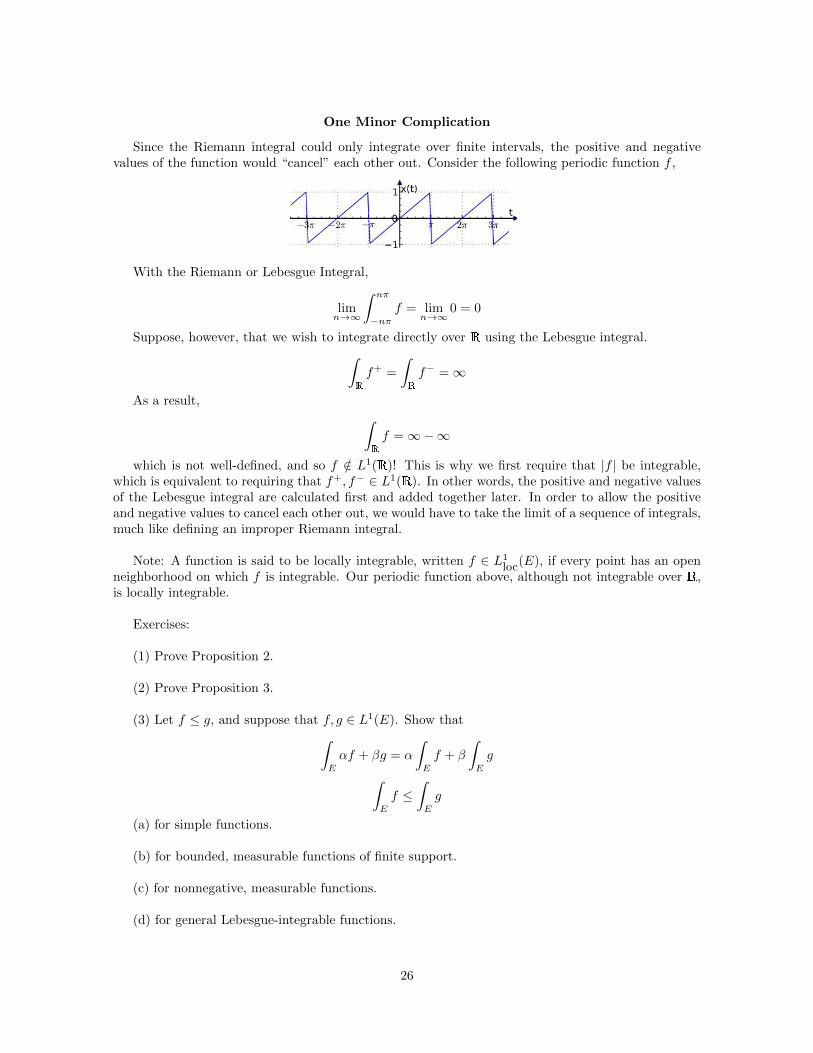
Since the Riemann integral could only integrate over finite intervals, the positive and negativevalues of the function would “cancel” each other out. Consider the following periodic function f ,
With the Riemann or Lebesgue Integral,
limn!1
Zn⇡
�n⇡
f = limn!1
0 = 0
Suppose, however, that we wish to integrate directly over using the Lebesgue integral.Z
f
+ =
Zf
� = 1As a result,
Zf = 1�1
which is not well-defined, and so f /2 L
1( )! This is why we first require that |f | be integrable,which is equivalent to requiring that f+
, f
� 2 L
1( ). In other words, the positive and negative valuesof the Lebesgue integral are calculated first and added together later. In order to allow the positiveand negative values to cancel each other out, we would have to take the limit of a sequence of integrals,much like defining an improper Riemann integral.
Note: A function is said to be locally integrable, written f 2 L
1loc
(E), if every point has an openneighborhood on which f is integrable. Our periodic function above, although not integrable over ,is locally integrable.
Exercises:
(1) Prove Proposition 2.
(2) Prove Proposition 3.
(3) Let f g, and suppose that f, g 2 L
1(E). Show thatZ
E
↵f + �g = ↵
Z
E
f + �
Z
E
g
Z
E
f Z
E
g
(a) for simple functions.
(b) for bounded, measurable functions of finite support.
(c) for nonnegative, measurable functions.
(d) for general Lebesgue-integrable functions.
26

(4) Let f be integrable over E, and let A and B are disjoint measurable subsets of E. Use theresult of problem (3), together with the � function, to show that
Z
A[B
f =
Z
A
f +
Z
B
f
(5) Show that if f, g 2 L
1(E), and f = g almost everywhere, thenZ
E
f =
Z
E
g
27
Measure Theory and Lebesgue Integration: Lesson VI
Besides for being good-looking and French, Pierre Fatou developed key resultsin Integration Theory and Complex Analytic Systems. In fact, Fatou was the first
mathematician to define the Mandelbrot set!
Pierre Fatou (1878 - 1929)
Lesson 6: Littlewood’s Three Principles. The Bounded and Uniform ConvergenceTheorems. Fatou’s Lemma and the Dominated and Monotone Convergence Theorems.
The theorems we are about to prove are a pretty big deal, and will make the Lebesgue integral agod-damned pleasure to work with. Trust me, once you’ve used the Lebesgue integral, there’s no goingback.
28

Littlewood’s Three Principles
In his 1944 text, Lectures on the Theory of Functions, J.E. Littlewood outlined three theorems thatgive great insight into the essentials of measure theory. These three principles give one an intuitiveway of thinking about measurable sets and functions, something that will prove invaluable as we makethe transition to advanced analysis. Due to the subtle and nontrivial nature of these proofs, I willrefrain from demonstrating them here, and will rather present only the results.
Principle One: Every measurable set of finite outer measure is almost the finite, disjoint unionof open intervals:
Let E 2 M such that m⇤(E) < 1. For each ✏ > 0, there exists a finite, disjoint collection of openintervals {I
k
}nk=1, with O =
Sn
k=1 Ik, such that
m
⇤(E4O) = m
⇤(E ⇠ O) +m
⇤(O ⇠ E) < ✏
Note: The symbol 4 above denotes the symmetric di↵erence of two sets. A4B consists of thosepoints that are either in A or B, but not both.
Principle Two (Egoro↵ ’s Theorem): Every pointwise-convergent sequence of measurable func-tions is nearly uniformly convergent:
Let E have finite measure, and let f
n
be a sequence of measurable functions converging to areal-valued function f on E. For every ✏ > 0, there exists a closed set F contained in E such thatm(E ⇠ F ) < ✏, and
f
n
! f uniformly on F
Principle Three (Lusin’s Theorem): Every measurable function is nearly continuous:
Let f be a real-valued measurable function on E. For any ✏ > 0, there exists a continuous functiong on and a closed set F ✓ E such that m(E ⇠ F ) < ✏ and f = g on F .
29

The following two convergence theorems are concerned with bounded functions of finite support.
Uniform Convergence Theorem
Let f
n
be a sequence of bounded, measurable functions on a set E of finite measure. If fn
! f
uniformly on E, then
limn!1
Z
E
f
n
=
Z
E
f
We refer to this as the passage of the limit under the integral sign.
Proof: Let ✏ > 0. Since our sequence converges uniformly to f , there must exist an N 2 suchthat
|fn
� f | < ✏
m(E)8n � N
Then, 8n � N ,����Z
E
(fn
� f)
���� Z
E
|fn
� f | <Z
E
✏
m(E)= ✏
m(E)
m(E)= ✏
Letting ✏! 0, the proof is complete. ⇤
Bounded Convergence Theorem
Let fn
be a sequence of measurable functions on a set E of finite measure. Furthermore, supposethat our sequence is uniformly bounded by some constant M , and that f
n
! f pointwise on E. Then
limn!1
Z
E
f
n
=
Z
E
f
Proof: They thrust of this proof is to appeal to Egoro↵ ’s Theorem to find a closed set F ✓ E
such that m(E ⇠ F ) < ✏ and f
n
converges uniformly on F . On F , we use the Uniform convergencetheorem to show that the di↵erence between the integrals can be made as small as we please. On theremaining set E ⇠ F , which has measure less than ✏, we use the fact that the f
n
(and f) are uniformlybounded to shrink the integral. Put rigorously,
����Z
E
(fn
� f)
���� Z
E
|fn
� f |
Z
F
|fn
� f |+Z
E⇠F
|fn
� f |
<
Z
F
|fn
� f |+ 2M✏
Letting n ! 1 and ✏! 0,Z
F
|fn
� f |+ 2M✏! 0
completing the proof. ⇤
30
Fatou’s Lemma
Let E be a measurable set, and let fn
be a sequence of nonnegative, measurable functions. Then
Z
E
lim inf fn
dx lim inf
Z
E
f
n
dx
If the f
n
converge to some function f , we can replace lim inf f with f .
Before we prove this theorem, let’s discuss why it makes sense.
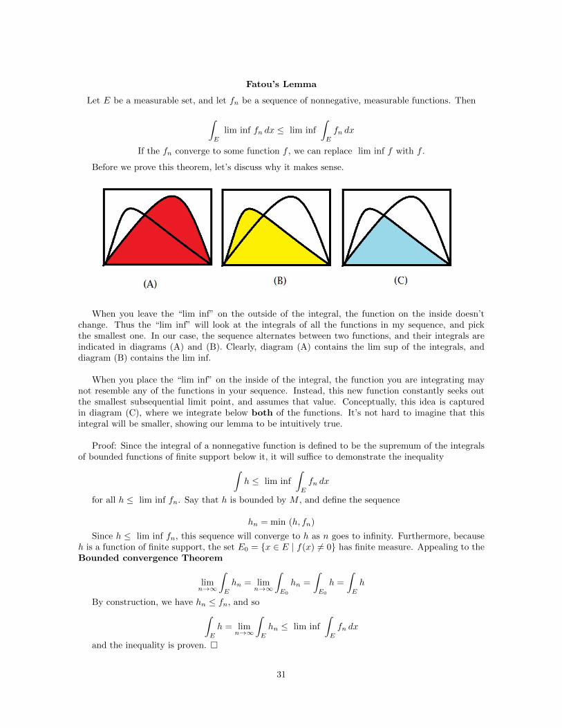
When you leave the “lim inf” on the outside of the integral, the function on the inside doesn’tchange. Thus the “lim inf” will look at the integrals of all the functions in my sequence, and pickthe smallest one. In our case, the sequence alternates between two functions, and their integrals areindicated in diagrams (A) and (B). Clearly, diagram (A) contains the lim sup of the integrals, anddiagram (B) contains the lim inf.
When you place the “lim inf” on the inside of the integral, the function you are integrating maynot resemble any of the functions in your sequence. Instead, this new function constantly seeks outthe smallest subsequential limit point, and assumes that value. Conceptually, this idea is capturedin diagram (C), where we integrate below both of the functions. It’s not hard to imagine that thisintegral will be smaller, showing our lemma to be intuitively true.
Proof: Since the integral of a nonnegative function is defined to be the supremum of the integralsof bounded functions of finite support below it, it will su�ce to demonstrate the inequality
Zh lim inf
Z
E
f
n
dx
for all h lim inf fn
. Say that h is bounded by M , and define the sequence
h
n
= min (h, fn
)
Since h lim inf fn
, this sequence will converge to h as n goes to infinity. Furthermore, becauseh is a function of finite support, the set E0 = {x 2 E | f(x) 6= 0} has finite measure. Appealing to theBounded convergence Theorem
limn!1
Z
E
h
n
= limn!1
Z
E0
h
n
=
Z
E0
h =
Z
E
h
By construction, we have h
n
f
n
, and soZ
E
h = limn!1
Z
E
h
n
lim inf
Z
E
f
n
dx
and the inequality is proven. ⇤
31

We shall now use Fatou’s Lemma to prove two convergence theorems of great utility.
Monotone Convergence Theorem (MCT)
Let f
n be an increasing sequence of nonnegative measurable functions on E. If fn
! f almosteverywhere on E, then
limn!1
Z
E
f
n
=
Z
E
f
Proof: Since f
n
f ,
lim sup
Z
E
f
n
Z
E
f
By Fatou’s Lemma,Z
E
f lim inf
Z
E
f
n
Combining these inequalities,
lim inf
Z
E
f
n
lim sup
Z
E
f
n
Z
E
f lim inf
Z
E
f
n
lim sup
Z
E
f
n
lim inf
Z
E
f
n
=
Z
E
f = lim sup
Z
E
f
n
limn!1
Z
E
f
n
=
Z
E
f ⇤
An Application of the MCT
If a function f is Lebesgue integrable, Chebyshev’s inequality bounds the size of the set onwhich it gets very large. However, it does not bound the value of the integral on the sets where f getslarge. It is possible that although the measure of the set is small, the value of the function is greatenough that the contribution of the integral on this set can remain substantial. To show that this isnot the case, use Chebyshev’s inequality to see that
limn!1
�{x2E|f(x)>n} = 0
Since f�{x2E|f(x)>n} f , we apply the MCT to conclude that
limn!1
Z
E
f�{x2E|f(x)>n} =
Z
E
0 = 0
And thus for any ✏ > 0, there exists a natural number N such thatZ
E
f�{x2E|f(x)>N} < ✏ ⇤
32

Dominated Convergence Theorem (DCT)
Let fn
be a sequence of measurable functions on E. Suppose that there exists a function g that isintegrable on E so that |f
n
| g. Such a function is said to dominate our sequence. If fn
! f almosteverywhere on E, then f is integrable on E, and
limn!1
Z
E
f
n
=
Z
E
f
Proof: g � f
n
is positive, so by Fatou’s Lemma,
Z
E
g � f
n
lim inf
Z
E
(g � f
n
) = lim inf
✓Z
E
g �Z
E
f
n
◆=
Z
E
g � lim sup
Z
E
f
n
Note that we switched from the “lim inf” to the “lim sup”, because the smallest value of the integraloccurs precisely when the f
n
are largest.
SubtractingRE
g from both sides, and dividing by �1, we find thatZ
E
f � lim sup
Z
E
f
n
Similarly,
Z
E
g + f
n
lim inf
Z
E
(g + f
n
) = lim inf
✓Z
E
g +
Z
E
f
n
◆=
Z
E
g + lim inf
Z
E
f
n
so thatZ
E
f lim inf
Z
E
f
n
Combining these inequalities, we see that
lim inf
Z
E
f
n
lim sup
Z
E
f
n
Z
E
f lim inf
Z
E
f
n
lim sup
Z
E
f
n
lim inf
Z
E
f
n
=
Z
E
f = lim sup
Z
E
f
n
limn!1
Z
E
f
n
=
Z
E
f ⇤
33

Here’s a rough outline of of the connection between the convergence theorems we’ve proven in thislesson.
Exercises:
1) Prove the Generalized Dominated Convergence Theorem. The statement is almost iden-tical to that of the DCT, expect we replace g with a sequence of nonnegative measurable functionsg
n
such that |fn
| g
n
. We also specify that the sequence convergence pointwise to some function g
almost everywhere on E, and that
limn!1
Z
E
g
n
=
Z
E
g 1
2) Let f be a nonnegative measurable function on . Show that
limn!1
Zn
�n
f =
Zf
(Taken from Royden’s Real Analysis)
3) Let f
n
be a sequence of integrable functions on E such that f
n
! f almost everywhere on E,and f is integrable on E. Show that
Z
E
|f � f
n
| ! 0
if and only if
limn!1
Z
E
|fn
| =Z
E
|f |
Hint: use the generalized DCT. (Taken from Royden’s Real Analysis)
34
Challenge Exercise: A function has compact support if the space on which it is nonzero is compact.We denote the space of continuous functions of compact support C0( ). Prove that C0( ) is dense inL
1 in the L
1 norm, i.e.
d(f, g) =
Z|f � g|
Hint: use Lusin’s Theorem, the Tietze Extension Theorem and a convergence theorem ofyour choice.
35

Measure Theory and Lebesgue Integration: Lesson VII
Lesson 7: The Riesz-Fischer Theorem: L
1 is complete.
When we began this course, we highlighted three concerns with the Riemann integral. The firstwas the large class of non-integrable functions, the second was the inability to integrate over infinitesets, and the third was the fact that R was not complete. We have shown that the Lebesgue integralcan integrate over almost any function we can imagine, and that it can be defined on sets of infinitemeasure. In the last lesson, we demonstrated a number of useful convergence theorems that make theLebesgue integral not only more versatile than its Riemann counterpart, but often easier to use. Tocomplete (no pun intended) our program of a finding “a better integral,” we will now show that L1 iscomplete, and hence a Banach space.
L
1 Convergence vs. Pointwise Convergence
Before we directly attempt the proof of the Riesz-Fischer theorem, we must take note of a potentialcomplication. For a sequence of functions to converge in the L
1 norm, it is not necessary that theyconverge pointwise almost-everywhere. In fact, they may not converge pointwise anywhere!
An example of this can be found in the following sequence of functions:
f
n,k
= �[ k�12n ,
k2n ] for n 2 , k 2 {1, · · · , 2n}
Here is a depiction of the first six terms in this sequence:
36

Each time we increment n, the length of the interval shrinks, and then as k ranges from 1 to 2n,that interval marches along [0, 1]. Clearly, the size of the integral gets smaller and smaller, so thissequence converges to 0 in the L
1 norm. Nevertheless, for any given point in [0, 1], our sequence ofintervals will continue to hit that point, no matter how large n and k become. Thus this sequencedoes not converge pointwise to 0 anywhere!
Note, however, that if we fix k = 1, we get a subsequence that converges pointwise to 0 almosteverywhere (except at the origin). This will be our line of attack: we will take our Cauchy sequence,extract an almost-everywhere-pointwise-convergent subsequence, and then apply the dominated con-vergence theorem to that.
Theorem (Riesz-Fischer) : Let fn
be a cauchy sequence of fuctions in L
1(E). Then f
n
convergesto some function f 2 L
1(E), and
limn!1
Z
E
f
n
=
Z
E
f
Proof: Since f
n
is a cauchy sequence, there exists some n(✏) 2 such that 8n � n(✏),Z
E
|fn
� f
n�1| < ✏
Now, define a subsequence n
k
= max (nk�1, n(1/2k)). We will show that this subsequence con-
verges pointwise almost everywhere. Set
g(x) = |fn1(x)|+
1X
k=1
|fnk+1 � f
nk |
Taking the integral,
Z
E
g =
Z
E
|fn1(x)|+
Z
E
1X
k=1
|fnk+1 � f
nk |
By the monotone convegence theorem, we can pull the integral into the summation (why?)
=
Z
E
|fn1(x)|+
1X
k=1
Z
E
|fnk+1 � f
nk |
Using the bounds that we built into our subsequence,
Z
E
|fn1(x)|+
1X
k=1
1
2k< 1
hence the sum defining g converges almost everywhere on E. This allows us to construct thefollowing function, certain that its summation will also converge almost everywhere.
f(x) = f
n1(x) +1X
k=1
�f
nk+1 � f
nk
�
Since |f | |g|, we can assert that f 2 L
1. To show that f
nk ! f in L
1, observe that the k
th
partial sum of f is
37

f
n1(x) +kX
i=1
�f
ni+1 � f
ni
�= f
nk+1
Since our summation converges almost everywhere, fnk ! f almost everywhere.
To see that
limn!1
Z
E
|fn
� f | = 0
we will use the dominated convergence theorem. We already know that |f | g, and
|fnk | =
�����fn1(x) +kX
i=1
�f
ni+1 � f
ni
������ |f
n1(x)|+kX
i=1
��f
ni+1 � f
ni
�� g(x)
which tells us that |fnk � f | < 2g, and so the dominated convergence theorem applies.
Lastly, because our sequence is Cauchy, if any subsequence converges to a function, the entiresequence converges to that function by the triangle inequality. ⇤
Exercises:
1) Let F be a subset of [0, 1], constructed in a similar manner to the Cantor Set. However, at thek
th step, instead of removing intervals of length 3�k, remove intervals of length ↵3�k, with 0 < ↵ < 1.Show that
(a) F is a closed set.
(b) [0, 1] ⇠ F is dense in [0, 1].
(c) m(F ) = 1� ↵
Such a set is called a Generalized Cantor Set.
2) Show that there is an open set of real numbers that has a boundary of positive measure. (Hint:consider the complement of the generalized Cantor Set).
3) Use the generalized Cantor Set to construct a Cauchy sequence of Riemann integrable functionsthat does not converge in R, using the L
1 norm.
4) Use the Riesz-Fisher theorem and the fact that C0( ) is dense in L
1 (from the previous set ofexercises) to show that the completion of R in the L
1 norm is L1.
fin
Thanks for reading!
38