Measure Theoretic Aspects Of Error Terms

By

Kamalakshya Mahatab

MATH10201005001

The Institute of Mathematical Sciences

A thesis submitted to theBoard of Studies in Mathematical Sciences

In partial fulfillment of requirementsfor the Degree of

DOCTOR OF PHILOSOPHYof

HOMI BHABHA NATIONAL INSTITUTE

April, 2016

arX

iv:1

605.

0188

7v1

[m

ath.

NT

] 6

May

201

6

STATEMENT BY THE AUTHOR

This dissertation has been submitted in partial fulfillment of requirements for an

advanced degree at Homi Bhabha National Institute (HBNI) and is deposited in the

Library to be made available to borrowers under rules of the HBNI.

Brief quotations from this dissertation are allowable without special permission,

provided that accurate acknowledgement of source is made. Requests for permission

for extended quotation from or reproduction of this manuscript in whole or in part

may be granted by the Competent Authority of HBNI when in his or her judgement

the proposed use of the material is in the interests of scholarship. In all other

instances, however, permission must be obtained from the author.

Date: Kamalakshya Mahatab

iii

DECLARATION

I, Kamalakshya Mahatab, hereby declare that the investigation presented in this

thesis has been carried out by me. The work is original and has not been submitted

earlier as a whole or in part for a degree or diploma at this or any other Institution

or University.

Date: Kamalakshya Mahatab

v

List of Publications

Journal

1. Kamalakshya Mahatab and Kannappan Sampath, Chinese Remainder The-

orem for Cyclotomic Polynomials in Z[X]. Journal of Algebra, 435 (2015),

Pages 223-262. doi:10.1016/j.jalgebra.2015.04.006.

2. Kamalakshya Mahatab, Number of Prime Factors of an Integer. Mathematics

News Letter, Ramanujan Mathematical Society, volume 24 (2013).

Others

1. Kamalakshya Mahatab and Anirban Mukhopadhyay, Measure Theoretic As-

pects of Oscillations of Error Terms. arXiv:1512.03144v1 (2015).

Available at: http://arxiv.org/pdf/1512.03144v1.pdf

Kamalakshya Mahatab

vii

Acknowledgments

First and foremost, I would like to express my sincere gratitude to my adviser

Prof. Anirban Mukhopadhyay for his continuous support and insightful guidance

throughout my thesis work. I have greatly benefited from his patience, many a times

he has listened to my naive ideas carefully and corrected my mistakes. In all my

needs, I always found him as a kind and helpful person. I am indebted to him for

all the care and help that I got from him during my Ph.D. time.

I am indebted to Prof. Amritanshu Prasad for initiating me into research. I have

learnt many beautiful mathematics while working under him on my M.Sc. thesis.

He has always encouraged me to think freely and has guided me on several research

projects.

Prof. Srinivas Kotyada was always available whenever I had any doubts. I sincerely

thank him for reading my mathematical writings patiently and giving his valuable

suggestions. In addition to being my teacher, he has been a loving and caring friend.

I am grateful to Prof. R. Balasubramanian for giving his valuable time to help

me understand several difficult concepts in number theory, Prof. Aleksandar Ivić

and Prof. Olivier Ramaré for their valuable suggestions while writing [28], Prof.

Gautami Bhowmik for initiating me to work on Omega theorems, and Prof. Vikram

Sharma for his help in writing [29].

I am also grateful to Prof. Partha Sarathi Chakraborty, Prof. D. S. Nagaraj, Prof. S.

Kesavan, Prof. K. N. Raghavan, Prof. S. Viswanath, Prof. Vijay Kodiyalam, Prof.

V. S. Sunder, Prof. Murali Srinivasan, Prof. Xavier Viennot, Prof. P. Sankaran,

Prof. Sanoli Gun, Prof. Kaneenika Sinha, Prof. Shanta Laishram, Prof. Stephan

Baier, Prof. A. Sankaranarayanan, Prof. Ritabrata Munshi, Prof. R. Thangadurai,

Prof. D. Surya Ramana, Prof. Gyan Prakash and many others for sharing their

mathematical insights through their beautiful lectures and courses.

I thank Dr. C. P. Anil Kumar for being a dear friend. During my first three years in

IMSc, I have always enjoyed my discussions with him which used to last for several

hours at a stretch.

I would also like to thank Kannappan Sampath, my first co-author [29] and a great

friend, for the many insightful mathematical discussions I had with him.

I would like to appreciate the inputs of Prateep Chakraborty, Krishanu Dan, Bhavin

Kumar Mourya, Prem Prakash Pandey, Senthil Kumar, Jaban Meher, Binod Kumar

Sahoo, Sachin Sharma, Kamal Lochan Patra, Neeraj Kumar, Geetha Thangavelu,

Sumit Giri, B. Ravinder, Uday Bhaskar Sharma, Akshaa Vatwani, Sudhir Pujahari

and Anish Mallick during the mathematical discussions that I had with them.

I am also indebted to my parents and my sister for their unconditional love and

emotional support, especially during the times of difficulties.

My stay at IMSc would not have been pleasant without my friends Sandipan De,

Mitali Routaray, Arghya Mondal, Chandan Maity, Issan Patri, Dibyakrupa Sa-

hoo, Archana Mishra, Mamta Balodi, Zodinmawia, Vivek M. Vyas, Ankit Agrawal,

Biswajit Ransingh, Ria Ghosh, Devanand T, Sneh Sinha, Kasi VIswanadham, Jay

Mehta, Dhriti Ranjan Dolai, Maguni Mahakhud, Keshab Bakshi, Priyamvad Srivas-

tav, Jyothsnaa Sivaraman, Narayanan P., G. Arun Kumar, Pranabesh Das, Meesum

x

Syed, Sridhar Narayanan and others. They have been a part of several beautiful

memories during my Ph.D.

Last, but not the least, I would like to thank my institute ‘The Institute of Math-

ematical Sciences’ for providing me a vibrant research environment. I have enjoyed

excellent computer facility, a well managed library, clean and well furnished hostel

and office rooms, and catering services at my institute. I would like to express my

special gratitude to the library and administrative staffs of my institute for their

efficient service.

Kamalakshya Mahatab

xi

Contents

Notations xv

Synopsis xvii

I Introduction 11 Framework . . . . . . . . . . . . . . . . . . . . . . . . . . . . . . . . . 32 Applications . . . . . . . . . . . . . . . . . . . . . . . . . . . . . . . . 4

2.1 Twisted Divisors . . . . . . . . . . . . . . . . . . . . . . . . . 52.2 Square Free Divisors . . . . . . . . . . . . . . . . . . . . . . . 62.3 Divisors . . . . . . . . . . . . . . . . . . . . . . . . . . . . . . 72.4 Error Term in the Prime Number Theorem . . . . . . . . . . . 82.5 Non-isomorphic Abelian Groups . . . . . . . . . . . . . . . . . 8

II Analytic Continuation Of The Mellin Transform 101 Perron’s Formula . . . . . . . . . . . . . . . . . . . . . . . . . . . . . 102 Analytic continuation of A(s) . . . . . . . . . . . . . . . . . . . . . . 13

2.1 Preparatory Lemmas . . . . . . . . . . . . . . . . . . . . . . . 132.2 Proof of Theorem 3 . . . . . . . . . . . . . . . . . . . . . . . . 18

3 Alternative Approches . . . . . . . . . . . . . . . . . . . . . . . . . . 18

III Landau’s Oscillation Theorem 211 Landau’s Criterion for Sign Change . . . . . . . . . . . . . . . . . . . 212 Ω± Results . . . . . . . . . . . . . . . . . . . . . . . . . . . . . . . . . 243 Measure Theoretic Ω± Results . . . . . . . . . . . . . . . . . . . . . . 274 Applications . . . . . . . . . . . . . . . . . . . . . . . . . . . . . . . . 33

4.1 Square Free Divisors . . . . . . . . . . . . . . . . . . . . . . . 334.2 The Prime Number Theorem Error . . . . . . . . . . . . . . . 36

IV Influence Of Measure 381 Refining Omega Result from Measure . . . . . . . . . . . . . . . . . . 392 Omega Plus-Minus Result from Measure . . . . . . . . . . . . . . . . 40

xiii

3 Applications . . . . . . . . . . . . . . . . . . . . . . . . . . . . . . . . 453.1 Error term of the divisor function . . . . . . . . . . . . . . . . 453.2 Average order of Non-Isomorphic abelian Groups . . . . . . . 47

V The Twisted Divisor Function 491 Applications of τ(n, θ) . . . . . . . . . . . . . . . . . . . . . . . . . . 49

1.1 Clustering of Divisors . . . . . . . . . . . . . . . . . . . . . . . 501.2 The Multiplication Table Problem . . . . . . . . . . . . . . . . 51

2 Asymptotic Formula for∑∗

n≤x |τ(n, θ)|2 . . . . . . . . . . . . . . . . . 523 Oscillations of the Error Term . . . . . . . . . . . . . . . . . . . . . . 534 An Omega Theorem . . . . . . . . . . . . . . . . . . . . . . . . . . . 56

4.1 Optimality of the Omega Bound . . . . . . . . . . . . . . . . 685 Influence of Measure on Ω± Results . . . . . . . . . . . . . . . . . . . 70

xiv

Notations

We denote the set of natural numbers by N, the set of integers by Z, the set ofreal numbers by R, the set of positive real numbers by R+, and the set of complexnumbers by C.

The notaion i stands for√−1, the square root of −1 that belongs to the upper half

plane in C.

We denote the Lebesgue mesure on the real line R by µ.

For z = σ + it ∈ C, we denote σ by <(z) and t by =(z).

Let f(x) and g(x) be a complex valued function on R+. As x→∞, we write

f(x) = O(g(x)), if limx→∞

∣∣∣f(x)g(x)

∣∣∣ > 0;

f(x) = o(g(x)), if limx→∞

∣∣∣f(x)g(x)

∣∣∣ = 0;

f(x) g(x), if f(x) = O(g(x));

f(x) g(x), if g(x) = O(f(x));

f(x) ∼ g(x), if limx→∞f(x)g(x)

= 1;

f(x) g(x), if 0 < limx→∞

∣∣∣f(x)g(x)

∣∣∣ <∞.

Let f(x) be a complex valued function on R+, and let g(x) be a positive monotonicfunction on R+. As x→∞, we write

f(x) = Ω(g(x)), if lim supx→∞|f(x)|g(x)

> 0;

f(x) = Ω+(g(x)), if lim supx→∞f(x)g(x)

> 0;

f(x) = Ω−(g(x)), if lim infx→∞f(x)g(x)

< 0;

f(x) = Ω±(g(x)), if f(x) = Ω+(g(x)) and f(x) = Ω−(g(x)).

xv

Synopsis

This thesis studies fluctuation of error terms that appears in various asymptoticformulas and size of the sets where these fluctuations occur. As a consequence, thisapproach replaces Landau’s criterion on oscillation of error terms.

General Theory

Consider a sequence of real numbers an∞n=1 having Dirichlet series

D(s) =∞∑n=1

anns,

which is convergent in some half-plane. As in Perron summation formula [37, II.2.1],we write

∗∑n≤x

an =M(x) + ∆(x),

whereM(x) is the main term, ∆(x) is the error term and∑∗ is defined as

∗∑n≤x

an =

∑n≤x an if x /∈ N,∑n<x an + 1

2ax if x ∈ N.

In this thesis, we obtain Ω and Ω± estimates for ∆(x). We shall use the Mellintransform of ∆(x) (defined below) to obtain such estimates.

Definition. The Mellin transform of ∆(x) be A(s), defined as

A(s) =

∫ ∞1

∆(x)

xs+1dx.

In this direction, under some natural assumptions and for a suitably definedcontour C , we shall show that

A(s) =

∫C

D(η)

η(s− η)dη.

xvii

In the above formula, the poles of D(s) that lie left to C are all the poles thatcontributes to the main termM(x). Landau [26] used the meromorphic continuationof A(s) to obtain Ω± results for ∆(x). He proved that if A(s) has a pole at σ0 + it0for some t0 6= 0 and has no real pole for s ≥ σ0, then

∆(x) = Ω±(xσ0).

We shall show a quantitative version of Landau’s theorem, which also generalizes atheorem of Gautami, Ramaré and Schlage-Puchta [6]. Below we state this theoremin a simplified way. We introduce the following notations to state these theorems.

Definition. Let

A+T (xσ0) := T ≤ x ≤ 2T : ∆(x) > λxσ0,A−T (xσ0) := T ≤ x ≤ 2T : ∆(x) < −λxσ0,AT (xσ0) := A+

T (xσ0) ∪ A−T (xσ0),

for some λ, σ0 > 0.

Theorem. Let σ0 > 0, and let the following conditions hold:

(1) A(s) has no real pole for <(s) ≥ σ0,

(2) there is a complex pole s0 = σ0 + it0, t0 6= 0, of A(s), and

(3) for positive functions h±(x) such that h± (x)→∞ as x→∞, we have∫A±T (xσ0 )

∆2(x)

x2σ0+1dx h±(T ).

Thenµ(A±T (xσ0)) = Ω

(T

h±(T )

),

where µ denotes the Lebesgue measure.

In the above theorem, Condition 2 is a very strong criterion. In the followingtheorem, we replace Condition 2 by an Ω-bound of µ(AT (xσ0)) and obtain an Ω±-result from the given Ω-bound.

Theorem. Let σ0 > 0, and let the following conditions hold:

(1) A(s) has no real pole for <(s) ≥ σ0, and

(2) µ(AT (xσ0)) = Ω(T 1−δ) for 0 < δ < σ0.

xviii

Then∆(x) = Ω±(T σ0−δ

′)

for any δ′ such that 0 < δ′ < δ.

The above two theorems are applicable to a wide class of arithmetic functions.Now we mention some results obtained by applying these theorems.

A Twisted Divisor Function

Given θ 6= 0, defineτ(n, θ) =

∑d|n

diθ.

The Dirichlet series of |τ(n, θ)|2 can be expressed in terms of Riemann zeta functionas

D(s) =∞∑n=1

|τ(n, θ)|2

ns=ζ2(s)ζ(s+ iθ)ζ(s− iθ)

ζ(2s)for <(s) > 1.

In [13, Theorem 33], Hall and Tenenbaum proved that

∗∑n≤x

|τ(n, θ)|2 = ω1(θ)x log x+ ω2(θ)x cos(θ log x) + ω3(θ)x+ ∆(x),

where ωi(θ)s are explicit constants depending only on θ. They also showed that

∆(x) = Oθ(x1/2 log6 x).

Here the main term comes from the residues of D(s) at s = 1, 1± iθ. All other polesof D(s) come from zeros of ζ(2s). Using a pole on the line <(s) = 1/4, Landau’smethod gives

∆(x) = Ω±(x1/4).

We prove the following bounds for a computable λ(θ) > 0 and for any ε > 0:

µ(T ≤ x ≤ 2T : ∆(x) > (λ(θ)− ε)x1/4

)= Ω

(T 1/2(log T )−12

),

µ(T ≤ x ≤ 2T : ∆(x) < (−λ(θ) + ε)x1/4

)= Ω

(T 1/2(log T )−12

).

For a constant c > 0, define

α(T ) =3

8− c

(log T )1/8.

xix

Applying a method due to Balasubramanian, Ramachandra and Subbarao [5], weprove

∆(T ) = Ω(Tα(T )

).

In fact, this method gives Ω-estimate for the measure of the sets involved:

µ(A ∩ [T, 2T ]) = Ω(T 2α(T )

),

whereA = x : |∆(x)| ≥Mxα(x)

and M > 0 is a positive constant. We also show that

either ∆(x) = Ω(xα(x)+δ/2

)or ∆(x) = Ω±

(x3/8−δ′

),

for 0 < δ < δ′ < 1/8. For any ε > 0, this result and the conjecture

∆(x) = O(x3/8+ε)

proves that∆(x) = Ω±(x3/8−ε).

Prime Number Theorem Error

Let an be the von Mandoldt function Λ(n):

Λ(n) :=

log p if n = pr, r ≥ 1, p prime ,0 otherwise.

.

Let∗∑

n≤x

Λn = x+ ∆(x).

From the Vinogradov’s zero free region for Riemann zeta function, one gets [23,Theorem 12.2]

∆(x) = O(x exp

(−c(log x)3/5(log log x)−1/5

))for some constant c > 0.

Hardy and Littlewood [15] proved that

∆(x) = Ω±(x1/2 log log log x

).

xx

But this result does not say about the measure of the sets, where the above Ω±bounds are attained by ∆(x). We obtain the following weaker result, but with anΩ-estimates for the measure of the corresponding sets.Let λ1 > 0 denotes a computable constant. For a fixed ε, 0 < ε < λ1, we write

A1 :=x : ∆(x) > (λ1 − ε)x1/2

,

A2 :=x : ∆(x) < (−λ1 + ε)x1/2

.

Then

µ([T, 2T ] ∩ Aj) = Ω(T 1−ε) , for j = 1, 2 and for any ε > 0.

Under Riemann Hypothesis, we have

µ([T, 2T ] ∩ Aj) = Ω

(T

(log T )4

)for j = 1, 2.

We also show the following unconditional Ω-bounds for the second moment of ∆:∫[T,2T ]∩Aj

∆2(x)dx = Ω(T 2) for j = 1, 2.

Non-isomorphic Abelian Groups

Let an denote the number of non-isomorphic abelian groups of order n. We write

∗∑n≤x

an =6∑

k=1

bkx1/k + ∆(x).

In the above formula, we define bk as

bk :=∞∏

j=1,j 6=k

ζ(j/k).

It is an open problem to show that

∆(x) x1/6+δ for any δ > 0. (1)

The best result on upper bound of ∆(x) is due to O. Robert and P. Sargos [33],which gives

∆(x) x1/4+ε for any ε > 0.

xxi

Also Balasubramanian and Ramachandra [4] proved that

∆(x) = Ω(x1/6

√log x

).

Following their method, we prove

µ(T ≤ x ≤ 2T : |∆(x)| ≥ λ2x

1/6(log x)1/2)

= Ω(T 5/6−ε),

for some λ2 > 0 and for any ε > 0. They also obtained

∆(x) = Ω±(x92/1221),

while it has been conjectured that

∆(x) = Ω±(x1/6−δ),

for any δ > 0. We shall show that either∫ 2T

T

∆4(x)dx = Ω(T 5/3+δ) or ∆(x) = Ω±(x1/6−δ),

for any 0 < δ < 1/42. The conjectured upper bound (1) of ∆(x) gives∫ 2T

T

∆4(x)dx T 5/3+δ.

This along with our result implies that

∆(x) = Ω±(x1/6−δ) for any 0 < δ < 1/42.

xxii

[ I ] Introduction

In 1896, Jacques Hadamard and Charles Jean de la Vallée-Poussin proved that thenumber of primes upto x is asymptotic to x/ log x. This result is well known as thePrime Number Theorem (PNT). Below we state a version of this theorem (PNT*)in terms of the von-Mangoldt function.

Definition 1. For n ∈ N, the von-Mangoldt function Λ(n) is defined as

Λ(n) =

log p if n = pr, r ∈ N and p prime,0 otherwise .

Theorem (PNT*). For a constant c1 > 0, we have

∗∑n≤x

Λ(n) = x+O(x exp

(−c1(log x)3/5(log log x)−1/5

)),

where∗∑

n≤x

Λ(n) =

∑n≤x Λ(n) if x /∈ N,∑n≤x Λ(n)− Λ(x)/2 otherwise .

For a proof of the above theorem see [23, Theorem 12.2]. Proof of PNT* usesanalytic continuation of the function

ζ(s) =∞∑n=1

1

ns,

defined for <(s) > 1. The function ζ(s) is called the ‘Riemann zeta function’, namedafter the famous German mathematician Bernhard Riemann. In 1859, Riemannshowed that this has a meromorphic continuation to the whole complex plane. Healso showed PNT by assuming that the meromorphic continuation of ζ(s) does nothave zeros for <(s) > 1

2. This conjecture of Riemann is popularly known as the

‘Riemann Hypothesis’ (RH), and is an unsolved problem. Under RH, the upperbound for ∆(x) in PNT* can be improved as in the following theorem:

1

Theorem (PNT**). Let ∆(x) be defined as in PNT*. Further, if we assume RH,then

∆(x) = O(x

12 log2 x

).

Proof. See [40].

In fact, we shall see in Theorem 6 that PNT** is equivalent to RH. At this point,it is natural to ask the following questions:

- Can we obtain a bound for ∆(x), better than the bound in PNT**?

- Is ∆(x) an increasing or a decreasing function?

- Can ∆(x) be both positive and negative depending on x?

- How large are positive and negative values of ∆(x)?

We shall make an attempt to answer these question by obtaining Ω and Ω± results.The following result was obtained by Hardy and Littlewood [15] in the year 1916:

∆(x) = Ω±

(x

12 log log log x

). (I.1)

The above Ω± bound on ∆(x) gives some answer to our earlier questions. It says thatwe can not have an upper bound for ∆(x) which is smaller than x

12 log log log x. It

also says that ∆(x) often takes both positive and negative values with magnitude oforder x

12 log log log x. This suggests, it is important to obtain Ω and Ω± bounds for

various other error terms. In this direction, Landau’s theorem [26] (see Theorem 6below) gives an elegant tool to obtain Ω± results. Applying this theorem, we have

∆(x) = Ω±

(x

12

).

The advantage of Landau’s method as compared to Hardy and Littlewood’s methodis in its applicability to a wide class of error terms of various summatory functions.In Landau’s method, the existence of a complex pole with real part 1

2serves as a

criterion for the existence of above limits. In this thesis, we shall investigate on aquantitative version of Landau’s result by obtaining the Lebesgue measure of thesets where ∆(x) > λx1/2 and ∆(x) < −λx 1

2 , for some λ > 0. We shall show thatthe large Lebesgue measure of the set where |∆(x)| > λx

12 , for some λ > 0 replaces

the criterion of existence of a complex pole in Landau’s method. This approach hasthe advantage of getting Ω± results even when no such complex pole exists. This isevident from some applications which we discuss in this thesis.

2

1 Framework

In this thesis, we consider a sequence of real numbers an∞n=1 having Dirichlet series

D(s) =∞∑n=1

anns

that converges in some half-plane. The Perron summation formula (see Theorem 1)uses analytic properties of D(s) to give

∗∑n≤x

an =M(x) + ∆(x),

where M(x) is the main term, ∆(x) is the error term ( which would be specifiedlater ) and

∑∗ is defined as

∗∑n≤x

an =

∑n≤x an if x /∈ N∑n≤x an −

12ax if x ∈ N.

In Chapter II, we analyze the Mellin transform A(s) of ∆(x), which is definedas:

Definition 2. For a complex variable s, the Mellin transform A(s) of ∆(x) is definedby

A(s) =

∫ ∞1

∆(x)

xs+1dx.

In general, A(s) is holomorphic in some half plane. We shall discuss a method toobtain a meromorphic continuation of A(s) from the meromorphic continuation ofD(s). In particular, we shall prove in Theorem 3 that under some natural assump-tions

A(s) =

∫C

D(η)

η(s− η)dη,

where the contour C is as in Definition 3 and s lies to the right of C . Later, thisresult will complement Theorem 9 and Theorem 11 in their applications.

In Chapter III, we revisit Landau’s method and obtain measure theoretic results.Also we generalize a theorem of Kaczorowski and Szydło [24], and a theorem ofBhowmik, Ramaré and Schlage-Puchta [6] in Theorem 11.

LetA(α, T ) := x : x ∈ [T, 2T ], |∆(x)| > xα,

3

and let µ denotes the Lebesgue measure on R. In Chapter IV, we establish aconnection between µ(A(α, T )) and fluctuations of ∆(x). In Proposition 3, we seethat

µ(A(α, T )) T 1−δ implies ∆(x) = Ω(xα+δ/2).

However, Theorem 13 gives that

µ(A(α, T )) = Ω(T 1−δ) implies ∆(x) = Ω±(xα−δ),

provided A(s) does not have a real pole for <(s) ≥ α − δ. In particular, this saysthat either we can improve on the Ω result or we can obtain a tight Ω± result for∆(x).

In Chapter V we study a twisted divisor function defined as follows:

τ(n, θ) =∑d|n

diθ for θ 6= 0. (I.2)

This function is used in [13, Chapter 4] to measure the clustering of divisors. Wegive a brief note on some applications of τ(n, θ) in Section V.1. In [13, Theorem33], Hall and Tenenbaum proved that

∗∑n≤x

|τ(n, θ)|2 = ω1(θ)x log x+ ω2(θ)x cos(θ log x) + ω3(θ)x+ ∆(x), (I.3)

where ωi(θ)s are explicit constants depending only on θ. They also showed that

∆(x) = Oθ(x1/2 log6 x). (I.4)

We give a proof of this formula in Theorem 14. Also, we derive Ω and Ω± bounds for∆(x) using techniques from previous chapters. In Theorem 15, we obtain an Ω boundfor the second moment of ∆(x) by adopting a technique due to Balasubramanian,Ramachandra and Subbarao [5].

The main theorems of this thesis, except Theorem 11, are from [28], which is ajoint work of the author with A. Mukhopadhyay.

2 Applications

Now we conclude the introduction by mentioning few applications of the methodsgiven in this thesis.

4

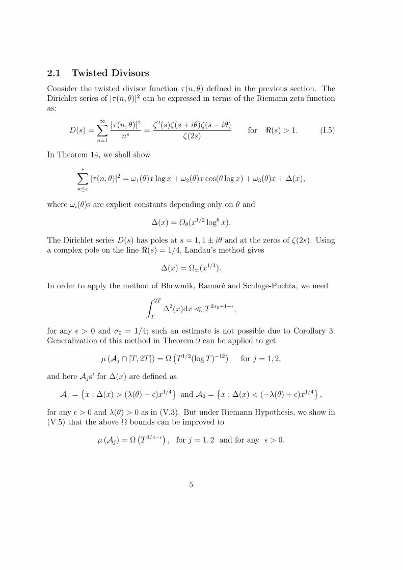
2.1 Twisted Divisors

Consider the twisted divisor function τ(n, θ) defined in the previous section. TheDirichlet series of |τ(n, θ)|2 can be expressed in terms of the Riemann zeta functionas:

D(s) =∞∑n=1

|τ(n, θ)|2

ns=ζ2(s)ζ(s+ iθ)ζ(s− iθ)

ζ(2s)for <(s) > 1. (I.5)

In Theorem 14, we shall show

∗∑n≤x

|τ(n, θ)|2 = ω1(θ)x log x+ ω2(θ)x cos(θ log x) + ω3(θ)x+ ∆(x),

where ωi(θ)s are explicit constants depending only on θ and

∆(x) = Oθ(x1/2 log6 x).

The Dirichlet series D(s) has poles at s = 1, 1± iθ and at the zeros of ζ(2s). Usinga complex pole on the line <(s) = 1/4, Landau’s method gives

∆(x) = Ω±(x1/4).

In order to apply the method of Bhowmik, Ramaré and Schlage-Puchta, we need∫ 2T

T

∆2(x)dx T 2σ0+1+ε,

for any ε > 0 and σ0 = 1/4; such an estimate is not possible due to Corollary 3.Generalization of this method in Theorem 9 can be applied to get

µ (Aj ∩ [T, 2T ]) = Ω(T 1/2(log T )−12

)for j = 1, 2,

and here Ajs’ for ∆(x) are defined as

A1 =x : ∆(x) > (λ(θ)− ε)x1/4

and A2 =

x : ∆(x) < (−λ(θ) + ε)x1/4

,

for any ε > 0 and λ(θ) > 0 as in (V.3). But under Riemann Hypothesis, we show in(V.5) that the above Ω bounds can be improved to

µ (Aj) = Ω(T 3/4−ε) , for j = 1, 2 and for any ε > 0.

5

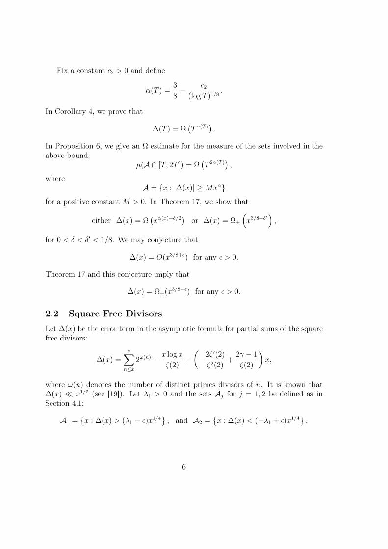
Fix a constant c2 > 0 and define

α(T ) =3

8− c2

(log T )1/8.

In Corollary 4, we prove that

∆(T ) = Ω(Tα(T )

).

In Proposition 6, we give an Ω estimate for the measure of the sets involved in theabove bound:

µ(A ∩ [T, 2T ]) = Ω(T 2α(T )

),

whereA = x : |∆(x)| ≥Mxα

for a positive constant M > 0. In Theorem 17, we show that

either ∆(x) = Ω(xα(x)+δ/2

)or ∆(x) = Ω±

(x3/8−δ′

),

for 0 < δ < δ′ < 1/8. We may conjecture that

∆(x) = O(x3/8+ε) for any ε > 0.

Theorem 17 and this conjecture imply that

∆(x) = Ω±(x3/8−ε) for any ε > 0.

2.2 Square Free Divisors

Let ∆(x) be the error term in the asymptotic formula for partial sums of the squarefree divisors:

∆(x) =∗∑

n≤x

2ω(n) − x log x

ζ(2)+

(−2ζ ′(2)

ζ2(2)+

2γ − 1

ζ(2)

)x,

where ω(n) denotes the number of distinct primes divisors of n. It is known that∆(x) x1/2 (see [19]). Let λ1 > 0 and the sets Aj for j = 1, 2 be defined as inSection 4.1:

A1 =x : ∆(x) > (λ1 − ε)x1/4

, and A2 =

x : ∆(x) < (−λ1 + ε)x1/4

.

6

In (III.14), we show that

µ (Aj ∩ [T, 2T ]) = Ω(T 1/2

)for j = 1, 2.

But under Riemann Hypothesis, we prove the following Ω bounds in (III.15):

µ (Aj ∩ [T, 2T ]) = Ω(T 1−ε) , for j = 1, 2 and for any ε > 0.

2.3 Divisors

Let d(n) denotes the number of divisors of n:

d(n) =∑d|n

1.

Dirichlet [17, Theorem 320] showed that

∗∑n≤x

d(n) = x log x+ (2γ − 1)x+ ∆(x),

where γ is the Euler constant and

∆(x) = O(√x).

Latest result on ∆(x) is due to Huxley [20], which is

∆(x) = O(x131/416).

On the other hand, Hardy [14] showed that

∆(x) = Ω+((x log x)1/4 log log x),

= Ω−(x1/4).

There are many improvements on Hardy’s result due to K. Corrádi and I. Kátai [7],J. L. Hafner [12] and K. Sounderarajan [36]. As a consequence of Theorem 13, weshall show in Chapter IV that for all sufficiently large T and for a constant c3 > 0,there exist x1, x2 ∈ [T, 2T ] such that

∆(x1) > c3x1 and ∆(x2) < −c3x2.

In particular, we get

∆(x) = Ω±(x1/4).

7

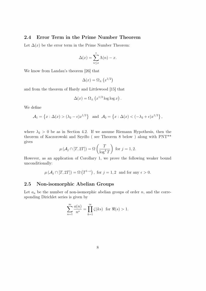
2.4 Error Term in the Prime Number Theorem

Let ∆(x) be the error term in the Prime Number Theorem:

∆(x) =∗∑

n≤x

Λ(n)− x.

We know from Landau’s theorem [26] that

∆(x) = Ω±(x1/2

)and from the theorem of Hardy and Littlewood [15] that

∆(x) = Ω±(x1/2 log log x

).

We define

A1 =x : ∆(x) > (λ2 − ε)x1/2

and A2 =

x : ∆(x) < (−λ2 + ε)x1/2

,

where λ2 > 0 be as in Section 4.2. If we assume Riemann Hypothesis, then thetheorem of Kaczorowski and Szydło ( see Theorem 8 below ) along with PNT**gives

µ (Aj ∩ [T, 2T ]) = Ω

(T

log4 T

)for j = 1, 2.

However, as an application of Corollary 1, we prove the following weaker boundunconditionally:

µ (Aj ∩ [T, 2T ]) = Ω(T 1−ε) , for j = 1, 2 and for any ε > 0.

2.5 Non-isomorphic Abelian Groups

Let an be the number of non-isomorphic abelian groups of order n, and the corre-sponding Dirichlet series is given by

∞∑n=1

a(n)

ns=∞∏k=1

ζ(ks) for <(s) > 1.

8

Let ∆(x) be defined as

∆(x) =∗∑

n≤x

an −6∑

k=1

(∏j 6=k

ζ(j/k))x1/k.

It is an open problem to show that

∆(x) x1/6+ε for any ε > 0. (I.6)

The best result on upper bound of ∆(x) is due to O. Robert and P. Sargos [33],which gives

∆(x) x1/4+ε for any ε > 0.

Balasubramanian and Ramachandra [4] proved that∫ 2T

T

∆2(x)dx = Ω(T 4/3 log T ).

Following the proof of Proposition 6, we get

µ(T ≤ x ≤ 2T : |∆(x)| ≥ λ3x

1/6(log x)1/2)

= Ω(T 5/6−ε),

for some λ2 > 0 and for any ε > 0. Sankaranarayanan and Srinivas [35] proved that

∆(x) = Ω±

(x1/10 exp

(c√

log x))

for some constant c > 0. It has been conjectured that

∆(x) = Ω±(x1/6−δ) for any δ > 0.

In Proposition 2, we prove that either∫ 2T

T

∆4(x)dx = Ω(T 5/3+δ) or ∆(x) = Ω±(x1/6−δ),

for any 0 < δ < 1/42. The conjectured upper bound (I.6) of ∆(x) gives∫ 2T

T

∆4(x)dx T 5/3+δ.

This along with Proposition 2 implies that

∆(x) = Ω±(x1/6−δ) for any 0 < δ < 1/42.

9

[ II ] Analytic Continuation Of The MellinTransform

In this chapter, we express the error term ∆(x) as a contour integral using thePerron’s formula. This allows us to obtain a meromorphic continuation of A(s) (seeDefinition 2) in terms of the meromorphic continuation of D(s), which is the maintheorem of this chapter ( Theorem 3 ). This theorem will be used in the next chapterto obtain Ω± results for ∆(x).

1 Perron’s Formula

Recall that we have a sequence of real numbers an∞n=1, with its Dirichlet seriesD(s). The Perron summation formula approximates the partial sums of an by ex-pressing it as a contour integral involving D(s).

Theorem 1 (Perron’s Formula, Theorem II.2.1 [37]). Let D(s) be absolutely con-vergent for <(s) > σc, and let κ > max(0, σc). Then for x ≥ 1, we have

∗∑n≤x

an =

∫ κ+i∞

κ−i∞

D(s)xs

sds.

But in practice, we use the following effective version of the Perron’s formula.

Theorem 2 (Effective Perron’s Formula, Theorem II.2.1 [37]). Let an∞n=1, D(s)and κ be defined as in Theorem 1. Then for T ≥ 1 and x ≥ 1, we have

∗∑n≤x

an =

∫ κ+iT

κ−iT

D(s)xs

sds+O

(xκ

∞∑n=1

|an|nκ(1 + T | log(x/n)|)

).

The above formulas are used by shifting the line of integration, and thus by collectingthe residues of D(s)xs/s at its poles lying to the right of the shifted contour. Theresidues contribute to the main term M(x), leaving an expression for ∆(x) as a

10

contour integral. So we write

∗∑n≤x

an =M(x) + ∆(x),

whereM(x) is the main term and ∆(x) is the error term. We make the followingnatural assumptions on D(s),M(x) and ∆(x).

Assumptions 1. Suppose there exist real numbers σ1 and σ2 satisfying 0 < σ1 < σ2,such that

(i) D(s) is absolutely convergent for <(s) > σ2.

(ii) D(s) can be meromorphically continued to the half plane <(s) > σ1 with onlyfinitely many poles ρ of D(s) satisfying

σ1 < <(ρ) ≤ σ2.

We shall denote this set of poles by P.

(iii) The main termM(x) is sum of residues of D(s)xs

sat poles in P:

M(x) =∑ρ∈P

Ress=ρ

(D(s)xs

s

).

The above assumptions also imply:

Note 1. We may also observe:

(i) For any ε > 0, we have

|an|, |M(x)|, |∆(x)|,

∣∣∣∣∣∑n≤x

an

∣∣∣∣∣ xσ2+ε.

(ii) The main termM(x) is a polynomial in x, and log x:

M(x) =∑j∈J

ν1,jxν2,j(log x)ν3,j ,

where ν1,j are complex numbers, ν2,j are real numbers with σ1 < ν2,j ≤ σ2, ν3,j

are positive integers, and J is a finite index set.

To express ∆(x) in terms of a contour integration, we define the following contour.

11

T0

0

−T0

σ1 σ2 σ3

C

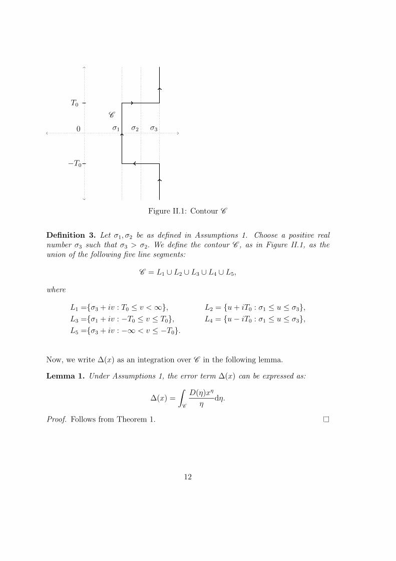
Figure II.1: Contour C

Definition 3. Let σ1, σ2 be as defined in Assumptions 1. Choose a positive realnumber σ3 such that σ3 > σ2. We define the contour C , as in Figure II.1, as theunion of the following five line segments:

C = L1 ∪ L2 ∪ L3 ∪ L4 ∪ L5,

where

L1 =σ3 + iv : T0 ≤ v <∞, L2 = u+ iT0 : σ1 ≤ u ≤ σ3,L3 =σ1 + iv : −T0 ≤ v ≤ T0, L4 = u− iT0 : σ1 ≤ u ≤ σ3,L5 =σ3 + iv : −∞ < v ≤ −T0.

Now, we write ∆(x) as an integration over C in the following lemma.

Lemma 1. Under Assumptions 1, the error term ∆(x) can be expressed as:

∆(x) =

∫C

D(η)xη

ηdη.

Proof. Follows from Theorem 1.

12

2 Analytic continuation of A(s)

Now, we shall discuss a method to obtain a meromorphic continuation of A(s),which will serve as an important tool to obtain Ω± results for ∆(x) in the followingchapter.Below we present the main theorem of this chapter.

Theorem 3. Under Assumptions-1, we have

A(s) =

∫C

D(η)

η(s− η)dη,

when s lies right to C .

2.1 Preparatory Lemmas

We shall need the following preparatory lemmas to prove the above theorem.From Lemma 1, we have:

A(s) =

∫ ∞1

∫C

D(η)xη

ηdη

dx

xs+1. (II.1)

To justify Theorem 3, we need to justify the interchange of the integrals of η and xin (II.1).

Definition 4. Define the following complex valued function B(s):

B(s) :=

∫C

D(η)

η

∫ ∞1

dx

xs−η+1dη

=

∫C

D(η)dη

(s− η)ηfor <(s) > <(η).

The integral defining B(s) being absolutely convergent, we have B(s) is welldefined and analytic.

Definition 5. For a positive integer N , define the contour C (N) as:

C (N) = η ∈ C : |=(η)| ≤ N.

Definition 6. Integrating the integrals of η and x, define BN(s) as:

BN(s) =

∫C (N)

D(η)dη

η

∫ ∞1

dx

xs−η+1

13

=

∫C (N)

D(η)dη

(s− η)ηfor <(s) > <(η).

With above definitions we prove:

Lemma 2. The functions B and BN satisfy the following identities:

B(s) = limN→∞

BN(s) (II.2)

= limN→∞

∫ ∞1

∫C (N)

D(η)xη

ηdη

dx

xs+1. (II.3)

Proof. Assume N > T0. To show (II.2), note:

|B(s)−BN(s)| ≤∣∣∣∣∫

C−C (n)

D(η)dη

(s− η)η

∣∣∣∣∣∣∣∣∫ σ3+i∞

σ3+iN

D(η)dη

(s− η)η+

∫ σ3−iN

σ3−i∞

D(η)dη

(s− η)η

∣∣∣∣∫ ∞N

dv

v2 1

N. ( substituting η = σ3 + iv)

This completes proof of (II.2).We shall prove (II.3) using a theorem of Fubini and Tonelli [8, Theorem B.3.1, (b)].

To show that the integrals commute, we need to show that one of the iterated inte-grals in (II.3) converges absolutely. We note:∫

C (N)

∫ ∞1

∣∣∣∣ D(η)

ηxs−η+1

∣∣∣∣ dx|dη|∫

C (N)

∣∣∣∣ D(η)

η(<(s)−<(η))

∣∣∣∣ |dη| <∞.This implies (II.3).

LetB′N(s) :=

∫ ∞1

∫C (N)

D(η)xη

ηdη

dx

xs+1. (II.4)

We re-write (II.3) of Lemma 2 as:

limN→∞

B′N(s) = B(s).

14

Observe that A(s) = B(s), if

limN→∞

∫ ∞1

∫C−C (N)

D(η)xη

ηdη

dx

xs+1= 0;

can be shown by interchanging the integral of x with the limit. For this, we need theuniform convergence of the integrand, which we do not have. It is easy to see fromTheorem 2 that the problem arises when x is an integer. To handle this problem,we shall divide the integral in two parts, with one part having neighborhoods ofintegers.

Definition 7. For δ = 1√N

( where N ≥ 2 ), we construct the following set as aneighborhood of integers:

S(δ) := [1, 1 + δ] ∪ (∪m≥2[m− δ,m+ δ]).

WriteA(s)−B′N(s) = J1,N(s) + J2,N(s)− J3,N(s), (II.5)

where

J1,N(s) =

∫S(δ)c

∫C−CN

D(η)xη

ηdη

dx

xs+1,

J2,N(s) =

∫S(δ)

∫ σ3+i∞

σ3−i∞

D(η)xη

ηdη

dx

xs+1,

J3,N(s) =

∫S(δ)

∫ σ3+iN

σ3−iN

D(η)xη

ηdη

dx

xs+1.

In the next three lemmas, we shall show that each of Ji,N(s)→ 0 as N →∞.

Lemma 3. For <(s) = σ > σ3 + 1, we have the limit

limN→∞

J1,N(s) = 0.

Proof. Using Theorem 2 with x ∈ S(δ)c, we have∣∣∣∣∫C−CN

D(η)xη

ηdη

∣∣∣∣ xσ3∞∑n=1

|an|nσ3(1 +N | log(x/n)|)

xσ3

N

∞∑n=1

|an|nσ3

+1

N

∑x/2≤n≤2x

x|an||x− n|

(xn

)σ3

15

xσ3

N+xσ3+1+ε

δN xσ3+1+ε

√N

( as δ = N−12 ).

From the above calculation, we see that

|J1,N | 1√N

∫ ∞1

xσ3−σ+εdx 1√N

for σ = <(s) > σ3 + 1 + ε. This proves our required result.

Lemma 4. For <(s) = σ > σ3,

limN→∞

J2,N(s) = 0.

Proof. Recall that

∗∑n≤x

an =

∑n<x an + ax/2 if x ∈ N,∑n≤x an if x /∈ N.

By Note 1,∗∑

n≤x

an xσ3 .

Using this bound, we calculate an upper bound for J2,N as follows:∣∣∣∣∫S(δ)

∫ σ3+i∞

σ3−i∞

D(η)xη

ηdη

dx

xs+1

∣∣∣∣ ≤ ∫S(δ)

∣∣∑∗n≤x an

∣∣xσ+1

dx

∫S(δ)

xσ3−σ−1dx∫ 1+δ

1

xσ3−σ−1 +∞∑m=2

∫ m+δ

m−δxσ3−σ−1dx.

This gives

|J2,N(s)| δ +∑m≥2

(1

(m− δ)σ−σ3− 1

(m+ δ)σ−σ3

).

Using the mean value theorem, for all m ≥ 2 there exists a real number m ∈[m− δ,m+ δ] such that

|J2,N(s)| δ +∑m≥2

δ

mσ−σ3+1 δ =1√N

by choosing σ > σ3.

This implies that J2,N → 0 as N →∞.

16

Lemma 5. For σ > σ3, we have

limN→∞

J3,N(s) = 0.

Proof. Consider

J3,N(s) =

∫S(δ)

∫ σ3+iN

σ3−iN

D(η)xη

ηdη

dx

xs+1.

This double integral is absolutely convergent for <(s) > σ3. Using the Theorem ofFubini and Tonelli [8, Theorem B.3.1, (b)], we can interchange the integrals:

J3,N(s) =

∫ σ3+iN

σ3−iN

D(η)

η

∫S(δ)

xη−s−1dx dη

=

∫ σ3+iN

σ3−iN

D(η)

η

∫ 1+δ

1

xη

xs+1dx+

∑m≥2

∫ m+δ

m−δ

xη

xs+1dx

dη.

For any θ1, θ2 such that 0 < θ1 < θ2 <∞, we have∫ θ2

θ1

xη−s−1dx =1

s− η

1

θs−η1

− 1

θs−η2

=θ2 − θ1

θs−η+1 ,

for some θ ∈ [θ1, θ2]. Applying the above formula to J3,N(s), we get

J3,N(s) =

∫ σ3+iN

σ3−iN

D(η)

η

∑m≥1

2δ

ms−η+1 dη = 2δ∑m≥1

∫ σ3+iN

σ3−iN

D(η)

ms−η+1ηdη,

where 1/2 ∈ [1, 1 + δ] and m ∈ [m − δ,m + δ] for all integers m ≥ 2. In the abovecalculation, we can interchange the series and the integral as the series is absolutelyconvergent. So we have

J3,N(s) δ∑m≥1

∫ N

−N

1

(1 + |v|)mσ−σ3+1 dv ( substituting η = σ3 + iv )

δ logN∑m≥1

1

mσ−σ3+1 logN√N

.

Here we used the fact that for σ > σ3, the series∑m≥1

1

ms−η+1

17

is absolutely convergent. This proves our required result.

2.2 Proof of Theorem 3

Proof. From equation (II.5) and Lemma 3, 4 and 5, we get

A(s) = limN→∞

B′N(s)

for <(s) > σ3 + 1, and where B′N(s) is defined by (II.4). From Lemma 2, we have

B(s) = limN→∞

B′N(s).

This gives A(s) and B(s) are equal for <(s) > σ3 + 1. By analytic continuation,A(s) and B(s) are equal for any s that lies right to C .

In this chapter, we shall use the meromorphic continuation of A(s) derived inTheorem 3 to obtain mesure theoretic Ω± results for ∆(x).

3 Alternative Approches

Theorem 3 gives a way for meromorphic continuation of A(s) by formulating itas a contour integral. This theorem has its significance in terms of elegance andgenerality. However, there are alternative and easier ways in many cases. Below wegive an example.

Note that∞∑n=1

anns

= −∫ ∞

1

(∑n≤x

an

)dx−s for <(s) > σ2.

This givesD(s)

s=

∫ ∞1

(∑n≤x

an

)x−s−1dx for <(s) > σ2.

So we can express A(s) as

A(s) =D(s)

s−∫ ∞

1

M(x)x−s−1dx for <(s) > σ2. (II.6)

The above formula reduces the problem of meromorphically continuing A(s) tothat of ∫ ∞

1

M(x)x−s−1dx.

18

To demonstrate this method, we consider the case when D(η) has a pole at η = 1and residue at this pole gives the main term M(x), i.e P = 1. The followingmeromorphic functions may serve as examples of D(η) in this situation:

ζ(s)

ζ(2s), ζ2(s),

ζ2(s)

ζ(2s),−ζ

′(s)

ζ(s), . . . .

For a small positive real number r, we can write M(x) as

M(x) =1

2πi

∫|η−1|=r

D(η)xη

ηdη.

Thus ∫ ∞1

M(x)

xs+1dx =

∫ ∞1

1

2πi

∫|η−1|=r

D(η)xη

ηdη

dx

xs+1

=1

2πi

∫|η−1|=r

D(η)

η

(∫ ∞1

dx

xs−η+1

)dη

( using [8, Theorem B.3.1, (b)] )

=1

2πi

∫|η−1|=r

D(η)

η(s− η)dη. (II.7)

Let the Laurent series expansion of D(η) at η = 1 be

D(η)

η=∑n≤N

bn(η − 1)n

+H(η),

where H(η) is holomorphic for <(η) > σ1. Plugging in this expression for D(η) in(II.7), we get ∫ ∞

1

M(x)

xs+1dx =

∑n≤N

bn1

2πi

∫|η−1|=r

dη

(η − 1)n(s− η). (II.8)

Let <(s) ≥ 1 + 2r, then

|η − 1||s− 1|

≤ 1

2for |η − 1| = r.

This gives1

s− η=∞∑n=0

(η − 1)n

(s− 1)n+1

19

is an absolutely convergent series. Using the above expansion of (s− η)−1 in (II.8),we have ∫ ∞

1

M(x)

xs+1dx =

∑n≤N

bn1

2πi

∫|η−1|=r

∞∑m=0

(η − 1)m

(s− 1)m+1

dη

(η − 1)n

=∑n≤N

bn(s− 1)n

( by [34, Theorem 6.1])

=D(s)

s−H(s).

Thus we gotA(s) = H(s) for <(s) ≥ 1 + 2r.

But the right hand side is holomorphic for <(s) > σ1 hence the formula gives analyticcontinuation of A(s) in the half plane Re(s) > σ1.

Similar calculations can be done when the main termM(x) is more complicated.

20

[ III ] Landau’s Oscillation Theorem

In this chapter, we revisit a result due to Landau and obtain Ω± results for ∆(x)using certain singularities of D(s). Also we shall measure the fluctuations of ∆(x)in terms of Ω bounds, which generalizes a result of Kaczorowski and Szydło [24],and a result of Bhowmik, Schlage-Puchta and Ramaré [6].

1 Landau’s Criterion for Sign Change

We begin with a result on real valued functions that do not change sign. Thisappears in a paper of Landau [26], attributed to Phragmén and stated without aproof. Here we present a proof of this result following [37, II.1.3, Theorem 6].

Theorem 4 (Phragmén-Landau). Let f(x) be a real valued piecewise continuousfunction defined for x ≥ 1, and bounded on every compact intervals. Let F (s) be itsMellin transform:

F (s) =

∫ ∞1

f(x)

xs+1dx,

converges absolutely in some complex right half plane. Also assume that f(x) doesnot change sign for x ≥ x0, for some x0 ≥ 1. If F (s) diverges for some real s, thenthere exist a real number σ0 satisfying the following properties:

(1) the integral defining F (s) is divergent for s < σ0 and convergent for s > σ0,

(2) s = σ0 is a singularity of F (s),

(3) and F (s) is analytic for <(s) > σ0.

Proof. Let σ0 be:σ0 = infσ ∈ R : F (σ) converges.

We shall show that σ0 satisfies the properties given in the theorem.As f(x) does not change sign for x ≥ x0, convergence of F (σ) implies the absolute

convergence of F (s) for <(s) ≥ σ. This proves (1) and (3). To prove (2), we proceedby method of contradiction. Assume that s = σ0 is not a singularity of F (s). Then

21

there exist σ′0 > σ0 and r > σ′0 − σ0 such that F (s) has the following Taylor seriesexpansion:

F (s) =∞∑k=0

1

k!F (k)(σ′0)(s− σ′0)k,

for all s satisfying |s− σ′0| < r.

Claim (1). For σ′0 as above, we have

F (s) =∞∑k=0

1

k!(s− σ′0)k

∫ ∞1

(− log x)kf(x)

xσ′0+1

dx.

Proof of Claim (1). By Cauchy’s integral formula, we can write

F (k)(σ′0) =k!

2πi

∫C

F (z)

(z − σ′0)k+1dz,

where C is a circle with a small enough radius having its center at σ′0. So we have

F (s) =∞∑k=0

(s− σ′0)k

2πi

∫C

1

(z − σ′0)k+1

∫ ∞1

f(x)

xz+1dx dz.

Suppose we can exchange the integrals of x and z, then

F (s) =∞∑k=0

(s− σ′0)k

k!

∫ ∞1

f(x)

x

k!

2πi

∫C

x−zdz

(z − σ′0)k+1dx

=∞∑k=0

1

k!(s− σ′0)k

∫ ∞1

(− log x)kf(x)

xσ′0+1

dx,

which proves Claim 1 conditionally. The only thing remains is to show that we canexchange integrals of x and z. If we choose C with a small enough radius, then∫ ∞

1

f(x)

x<(z)+1dx

is absolutely convergent and so is the double integral∫C

1

(z − σ′0)k+1

∫ ∞1

f(x)

xz+1dx dz.

By the theorem of Fubinni and Tonelli [8, Theorem B.3.1, (b)], we can exchangethese two iterated integrals. This completes the proof of Claim 1.

22

Claim (2). For |s− σ′0| < r, the integral

F (s) =

∫ ∞1

f(x)

xs+1dx

converges.

Proof of Claim (2). We shall simplify F (s) using Claim 1. We write

F (s) =∞∑k=0

(σ′0 − s)k

k!

∫ ∞1

(log x)kf(x)

xσ′0+1

dx.

In the above identity, we can exchange the series and the integral as the series isabsolutely convergent. So we have∫ ∞

1

f(x)

xσ′0+1

(∞∑k=0

(σ′0 − s)k

k!(log x)k

)dx

=

∫ ∞1

f(x)

xσ′0+1

exp((σ′0 − s) log x)dx =

∫ ∞1

f(x)

xs+1dx.

This completes the proof of Claim 2.But Claim 2 implies that we have a real number smaller than σ0, say σ′′0 , such

that the integral of F (σ′′0) converges. This is a contradiction to the definition of σ0.So σ0 is a singularity of F (s), which proves (2).

The following theorem appears in [1, Section 2] without a proof and is attributedto Landau. We shall prove this theorem using Theorem 4.

Theorem 5 (Phragmén-Landau-Anderson-Stark ). Let f(x) be a real valued piece-wise continuous function defined on [1,∞), bounded on every compact intervals, anddoes not change sign when x > x0 for some 1 < x0 <∞. Define

F (s) :=

∫ ∞1

f(x)

xs+1dx,

and assume that the above integral is absolutely convergent in some half plane. Fur-ther, assume that we have an analytic continuation of F (s) in a region containinga part of the real line

l(σ0,∞) := σ + i0 : σ > σ0.

Then the integral representing F (s) is absolutely convergent for <(s) > σ0, andhence F (s) is an analytic function in this region.

23

Proof. By Theorem 4, if ∫ ∞1

f(x)

xσ′+1dx

diverges for some σ′ > σ0, then there exist a real number σ′0 ≥ σ′ > σ0 such thatF is not analytic at σ′0. But this contradicts our assumption that F is analytic onl(σ0,∞). So the integral∫ ∞

1

f(x)

xσ′+1dx converges ∀ σ′ > σ0,

and since f does not change sign for x ≥ x0, F (s) converges absolutely for <(s) > σ0.This also gives that F (s) is analytic for <(s) > σ0.

The above two theorems give some criteria when a function does not change sign.In the next section we will use these results to show the sign changes of ∆(x).

2 Ω± Results

Consider the Mellin transform A(s) of ∆(x). We need the following assumptions toapply Theorem 5.

Assumptions 2. Suppose there exists a real number σ0, 0 < σ0 < σ1, such thatA(s) has the following properties.

(i) There exists t0 6= 0 such that

λ := lim supσσ0

(σ − σ0)|A(σ + it0)| > 0.

(ii) At σ0 we have

ls := lim supσσ0

(σ − σ0)A(σ) <∞,

li := lim infσσ0

(σ − σ0)A(σ) > −∞.

(iii) The limits li, ls and λ satisfy

li + λ > 0 and ls − λ < 0.

(iv) We can analytically continue A(s) in a region containing the real line l(σ0,∞).

Remark 1. From Assumptions 2,(i), we see that σ0 + it0 is a singularity of A(s).

24

We construct the following sets for further use.

Definition 8. With ls, li and λ as in Assumptions 2 and for an ε such that 0 < ε <min(li + λ, λ− ls), define

A1 := x : x ∈ [1,∞),∆(x) > (li + λ− ε)xσ0,and A2 := x : x ∈ [1,∞),∆(x) < (ls − λ+ ε)xσ0.

Under Assumptions 2 and using methods from [24], we can derive the followingmeasure theoretic theorem.

Theorem 6. Let the conditions in Assumptions 2 hold. Then for any real numberM > 1, we have

µ(A1 ∩ [M,∞]) > 0,

and µ(A2 ∩ [M,∞]) > 0.

This implies

∆(x) = Ω±(xσ0).

Proof. We prove the Theorem only for A1 as the other part is similar.Define

g(x) := ∆(x)− (li + λ− ε)xσ0 , G(s) :=

∫ ∞1

g(x)

xs+1dx;

g+(x) := max(g(x), 0), G+(s) :=

∫ ∞1

g+(x)

xs+1dx;

g−(x) := max(−g(x), 0), G−(s) :=

∫ ∞1

g−(x)

xs+1dx.

With the above notations, we have

g(x) = g+(x)− g−(x),

and G(s) = G+(s)−G−(s).

Note that

G(s) = A(s)−∫ ∞

1

(li + λ− ε)xσ0−s−1dx

= A(s) +li + λ− εσ0 − s

, for <(s) > σ0.

25

So G(s) is analytic wherever A(s) is, except possibly for a pole at σ0. This gives

lim supσσ0

(σ − σ0)|G(σ + it0)| = lim supσσ0

(σ − σ0)|A(σ + it0)| = λ. (III.1)

We shall use the above limit to prove our theorem. We proceed by method ofcontradiction. Assume that there exists an M > 1 such that

µ(A1 ∩ [M,∞)) = 0.

This implies

G+(σ) =

∫ ∞1

g+(x)

xs+1dx =

∫ M

1

g+(x)

xs+1dx

is bounded for any s, and so is an entire function. By Assumptions 2, A(s) and G(s)can be analytically continued on the line l(σ0,∞). As G(s) and G+(s) are analyticon l(σ0,∞), G−(s) is also analytic on l(σ0,∞). The integral for G−(s) is absolutelyconvergent for <(s) > σ3 + 1, and g−(x) is a piecewise continuous function boundedon every compact sets. This suggests that we can apply Theorem 5 to G−(s), andconclude that

G−(s) =

∫ ∞1

g−(x)

xs+1dx

is absolutely convergent for <(s) > σ0.From the above discussion, we summarize that the Mellin transforms of g, g+ and

g− converge absolutely for <(s) > σ0. As a consequence, we see that G(σ), G+(σ)and G−(σ) are finite real numbers for σ > σ0. For σ > σ0, we compare G+(σ) andG−(σ) in the following two cases.

Case 1: G+(σ) < G−(σ).

In this case,

(σ − σ0)|G(σ + it0)| ≤ (σ − σ0)|G(σ)|= −(σ − σ0)G(σ)

= −(σ − σ0)A(σ) + li + λ− ε.

So we have

lim supσσ0

(σ − σ0)|G(σ + it0)| ≤ li + λ− ε− lim infσσ0

(σ − σ0)A(σ) ≤ λ− ε.

This contradicts (III.1).

Case 2: G+(σ) ≥ G−(σ).

26

We have,

(σ − σ0)|G(σ + it0)| ≤ (σ − σ0)G+(σ)

= O(σ − σ0) (G+(σ) being a bounded integral).

Thuslim supσσ0

(σ − σ0)|G(σ + it0)| = 0.

This contradicts (III.1) again.

Thus µ(A1 ∩ [M,∞)) > 0 for any M > 1, which completes the proof.

3 Measure Theoretic Ω± Results

Now we know that A1 and A2 are unbounded. But we do not know how the size ofthese sets grow. An answer to this question was given by Kaczorowski and Szydłoin [24, Theorem 4].

Theorem 7 (Kaczorowski and Szydło [24]). Let the conditions in Assumptions 2hold. Also assume that for a non-decreasing positive continuous function h satisfying

h(x) xε,

we have ∫ 2T

T

∆2(x)dx T 2σ0+1h(T ). (III.2)

Then as T →∞,

µ (Aj ∩ [1, T ]) = Ω( T

h(T )

)for j = 1, 2.

In [24], Kaczorowski and Szydło applied this theorem to the error term appearingin the asymptotic formula for the fourth power moment of Riemann zeta function.We write this error term as E2(x):∫ x

0

∣∣∣∣ζ (1

2+ it

)∣∣∣∣4 dt = xP (log x) + E2(x),

where P is a polynomial of degree 4. Motohashi [31] proved that

E2(x) x2/3+ε,

27

and further in [32] he showed that

E2(x) = Ω±(√x).

Theorem of Kaczorowski and Szydło ( Theorem 8 ) gives that there exist λ0, ν > 0such that

µ1 ≤ x ≤ T : E2(x) > λ0

√x = Ω(T/(log T )ν)

andµ1 ≤ x ≤ T : E2(x) < −λ0

√x = Ω(T/(log T )ν)

as T →∞. These results not only prove Ω±-results, but also give quantitative esti-mates for the occurrences of such fluctuations. The above theorem of Kaczorowskiand Szydło has been generalized by Bhowmik, Ramaré and Schlage-Puchta by lo-calizing the fluctuations of ∆(x) to [T, 2T ]. Proof of this theorem follows from [6,Theorem 2] (also see Theorem 10 below).

Theorem 8 (Bhowmik, Ramaré and Schlage-Puchta [6]). Let the assumptions inTheorem 7 hold. Then as T →∞,

µ (Aj ∩ [T, 2T ]) = Ω( T

h(T )

)for j = 1, 2.

An application of the above theorem to Goldbach’s problem is given in [6]. Let

∑n≤x

Gk(n) =xk

k!− k

∑ρ

xk−1+ρ

ρ(1 + ρ) · · · (k − 1 + ρ)+ ∆k(x),

where the Goldbach numbers Gk(n) are defined as

Gk(n) =∑

n1,...nkn1+···+nk=n

Λ(n1) · · ·Λ(nk),

and ρ runs over nontrivial zeros of the Riemann zeta function ζ(s). Bhowmik,Ramaré and Schlage-Puchta proved that under Riemann Hypothesis

µT ≤ x ≤ 2T : ∆k(x) > (ck + c′k)xk−1 = Ω(T/(log T )6)

and µT ≤ x ≤ 2T : ∆k(x) < (ck − c′k)xk−1 = Ω(T/(log T )6) as T →∞,

where k ≥ 2 and ck, c′k are well defined real number depending on k with c′k > 0.

Note that Theorem 7 implies Theorem 8, but both the theorems are applicableto the same set of examples. The main obstacle in applicability of these theoremsis the condition (III.2). For example, if ∆(x) is the error term in approximating

28

∑n≤x |τ(n, θ)|2, we can not apply Theorem 7 and Theorem 8. However, the following

theorem due to the author and A. Mukhopadhyay [28, Theorem 3] overcomes thisobstacle by replacing the condition (III.2).

Theorem 9. Let the conditions in Assumptions 2 hold. Assume that there is ananalytic continuation of A(s) in a region containing the real line l(σ0,∞). Let h1

and h2 be two positive functions such that∫[T,2T ]∩Aj

∆2(x)

x2σ0+1dx hj(T ) for j = 1, 2. (III.3)

Then as T −→∞,

µ(Aj ∩ [T, 2T ]) = Ω( T

hj(T )

)for j = 1, 2. (III.4)

Below we state an integral version of Theorem 8 as in [6].

Theorem 10 (Bhowmik, Ramaré and Schlage-Puchta [6]). Suppose the conditionsin Assumptions 2 hold, and let h(x) be as in Theorem 8. Then as δ → 0+,∫ ∞

1

µ(Aj ∩ [x, 2x])h(4x)

x2+δdx = Ω

(1

δ

), for j = 1, 2.

In our next theorem, we generalize Theorem 7, 8, 9 and 10.

Theorem 11. Let the conditions in Theorem 9 hold. Then as δ → 0+,∫ ∞1

µ(Aj ∩ [x, 2x])hj(x)

x2+δdx = Ω

(1

δ

)for j = 1, 2. (III.5)

Proof. We shall prove the theorem for j = 1; the proof is similar for j = 2. Wedefine g, g+, g−, G,G+ and G−, as in Theorem 6. Let

m#(x) := h1(x)µ(A1 ∩ [x, 2x])x−1.

First, we shall show:

Claim (1). As δ → 0, ∑k≥0

m#(2k)

2kδ= Ω

(1

δ

).

Assume that ∑k≥0

m#(2k)

2kδ= o

(1

δ

). (III.6)

29

From the above assumption, we may obtain an upper bound for G+(σ) as follows:∫A1

g+(x)dx

xσ+1≤∑k≥0

∫A1∩[2k,2k+1]

∆(x)dx

xσ+1(as ∆(x) > g(x) on A1)

≤∑k≥0

(∫A1∩[2k,2k+1]

∆2(x)dx

x2σ0+1

) 12(µ(A1 ∩ [2k, 2k+1])

2k(2δ+1)

) 12

(where σ − σ0 = δ > 0)

≤ c3

∑k≥0

(h1(2k)µ(A1 ∩ [2k, 2k+1])

2k(2δ+1)

) 12

≤ c3

∑k≥0

(m#(2k)

22kδ

) 12

.

From the above inequality, we get

δG+(σ) δ

(∑k≥0

1

2kδ

) 12(∑k≥0

m#(2k)

2k(σ−σ0)

) 12

= o(1) (III.7)

as δ → 0+. ThereforeG+(s) =

∫ ∞1

g+(x)dx

xs+1

is absolutely convergent for <(s) > σ0, and so it is analytic in this region. But

G−(s) = G(s)−G+(s),

and G is analytic on l(σ0,∞). So G− is also analytic on l(σ0,∞). Using Theorem 5,we get

G+(s) =

∫ ∞1

g+(x)dx

xs+1

is absolutely convergent for <(s) > σ0. Absolute convergence of the integrals of Gand G+ implies that the Mellin transformation of g−(x), given by

G−(s) =

∫ ∞1

g−(x)dx

xs+1,

is also absolutely convergent for <(s) > σ0. As a consequence, we get G(σ), G+(σ),and G−(σ) are finite non-negative real numbers for σ > σ0. As indicated in Case-1of Theorem 6, we can not have

G+(σ) < G−(σ) when σ > σ0.

So we always haveG+(σ) ≥ G−(σ).

30

Using (III.7),

lim supσσ0

(σ − σ0)|G(σ + it0)| ≤ lim supσσ0

(σ − σ0)G(σ) = 0.

This is a contradiction to (III.1), and so (III.6) is wrong. This proves our Claim.Now we are ready to prove the theorem. For k ≥ 1, observe that∫ k

k−1

m#(2x)

2δxdx =

∫ k

k−1

h1(2x)µ(A1 ∩ [2x, 2x+1])

2x(δ+1)dx =

∫ k

k−1

∫ 2x+1

2x

h1(2x)

2δx+xdA1(t)dx

(where A1(t) is the indicator function of A1)

=

∫ 2k

2k−1

∫ log tlog 2

k−1

h1(2x)

2x(1+δ)dxdA1(t) +

∫ 2k+1

2k

∫ k

log tlog 2−1

h1(2x)

2x(1+δ)dxdA1(t)

From the above identity, we have∫ k

k−1

m#(2x)

2δxdx ≥

∫ 2k+1

2k

∫ k

log tlog 2−1

h1(2x)

2x(1+δ)dxdA1(t)

and ∫ k+1

k

m#(2x)

2δxdx ≥

∫ 2k+1

2k

∫ log tlog 2

k

h1(2x)

2x(1+δ)dxdA1(t).

So we get∫ k+1

k−1

m#(2x)

2δxdx ≥

∫ 2k+1

2k

∫ k

log tlog 2−1

h1(2x)

2x(1+δ)dxdA1(t) +

∫ 2k+1

2k

∫ log tlog 2

k

h1(2x)

2x(1+δ)dxdA1(t)

=

∫ 2k+1

2k

∫ log tlog 2

log tlog 2−1

h1(2x)

2x(1+δ)dxdA1(t).

Now, we may use the fact that h1 is a monotonically increasing function havingpolynomial growth, and simplify the above calculation as follows:∫ k+1

k−1

m#(2x)

2δxdx ≥ h1(2k)

∫ 2k+1

2k

∫ log tlog 2

log tlog 2−1

dx

2x(1+δ)dA1(t)

=h1(2k)

log 2

∫ 2k+1

2k

(2−( log t

log 2−1)(1+δ) − 2−

log tlog 2

(1+δ))

dA1(t)

31

=h1(2k)

log 2

∫ 2k+1

2k

21+δ − 1

t1+δdA1(t) ≥ h1(2k)

2(k+1)(δ+1)µ(A1 ∩ [2k, 2k+1]) ≥ 1

4

m#(2k)

2kδ.

(III.8)

Now using Claim (1), we get∫ ∞0

m#(2x)

2δxdx

∞∑k=1

m#(2k)

2kδ= Ω

(1

δ

).

Changing the variable x to u = 2x in the above inequality gives

1

log 2

∫ ∞1

m#(u)

u1+δdu = Ω

(1

δ

),

or∫ ∞

1

µ(Aj ∩ [u, 2u])hj(u)

u2+δdu = Ω

(1

δ

).

This proves the theorem.

Corollary 1. Let the conditions given in Theorem 9 hold. Suppose we have amonotonically increasing positive function h such that

∆(x) = O(h(x)), (III.9)

thenµ(Aj ∩ [T, 2T ]) = Ω

(T 1+2σ0

h2(T )

)for j = 1, 2. (III.10)

Corollary 2. Similar to Corollary 1, we assume that the conditions in Theorem 9hold. Then we have∫

[T,2T ]∩Aj∆2(x)dx = Ω(T 2σ0+1) for j = 1, 2. (III.11)

Proof. This Corollary follows from the proof of Theorem 11. We shall prove thisCorollary for A1, and the proof for A2 is similar. Note that in the proof of Theo-rem 11, we showed that the integral for G+(s) is absolutely convergent for <(s) > σ0

by assuming (III.6). Then we got a contradiction which proves Claim (1) of Theo-rem 11. Now we proceed in a similar manner by assuming (III.11) is false. So wehave ∫

[T,2T ]∩A1

∆2(x)dx = o(T 2σ0+1).

32

So for an arbitrarily small constant ε, we have

|G+(s)| ≤∫A1

g+(x)dx

xσ+1≤∑k≥0

∫A1∩[2k,2k+1]

∆(x)dx

xσ+1

≤∑k≥0

1

2k(σ−σ0)

(∫A1∩[2k,2k+1]

∆2(x)dx

x2σ0+1

)1/2

≤ c4(ε) + ε∑k≥k(ε)

1

2k(σ−σ0),

where c4(ε) is a positive constant depending on ε. From this we obtain that G+(s)is absolutely convergent for <(s) > σ0. Now onwards the proof is same as that ofTheorem 11.

4 Applications

Now we demonstrate applications of our theorems in the previous section to errorterms appearing in two well known asymptotic formulas.

4.1 Square Free Divisors

Let an = 2ω(n), where ω(n) denotes the number of distinct prime factors of n;equivalently, an denotes the number of square free divisors of n. We write

∗∑n≤x

2ω(n) =M(x) + ∆(x),

whereM(x) =

x log x

ζ(2)+

(−2ζ ′(2)

ζ2(2)+

2γ − 1

ζ(2)

)x,

and by a theorem of Hölder [19]

∆(x) x1/2. (III.12)

Under Riemann Hypothesis, Baker [2] has improved the above upper bound to

∆(x) x4/11.

33

0 1

s0

54

14

34

15

−2

2

14

Figure III.1: Contours for square-free divisors.

It is easy to see that the Dirichlet series D(s) has the following form:

D(s) =∞∑n=1

2ω(n)

ns=ζ2(s)

ζ(2s).

Let A(s) be the Mellin transform of ∆(x) at s, and let s0 be the zero of ζ(2s) withleast positive imaginary part:

2s0 =1

2+ i14.134 . . . . (III.13)

We define a contour C (1) as union of the following five lines:

C (1) :=

(5

4− i∞, 5

4− i2

]∪[

5

4− i2, 3

4− i2

]∪[

3

4− i2, 3

4+ i2

]∪[

3

4+ i2,

5

4+ i2

]∪[

5

4+ i2,

5

4+ i∞

)The contour C (1) is represented by ‘dashed’ lines in Figure III.1. By Theorem 3, wehave

A(s) =

∫ ∞1

∆(x)

xs+1dx =

∫C (1)

D(η)

η(s− η)dη.

34

Now, we shift the contour C (1) to form a new contour C (2), so that

1, s0, l

(1

4,∞)

lie to the right of C (2). We have represented the contour C (2) by dotted lines inFigure III.1.

Since s0 is a pole of D(s) and is on the right side of C (1), we have

A(s) =

∫C (2)

D(η)

η(s− η)dη + Res

η=s0

(D(η)

η(s− η)

).

From the above formula, we may compute the following limits:

λ1 := limσ0

σ|A(σ + s0)| = |s0|−1

∣∣∣∣Resη=s0D(η)

∣∣∣∣ > 0

andlimσ0

σA(σ + 1/4) = 0.

For a fixed ε0 > 0,

A1 =x : ∆(x) > (λ1 − ε0)x1/4

and A2 =

x : ∆(x) < (−λ1 + ε0)x1/4

.

Using Corollary 1 and (III.12), we get

µ (Aj ∩ [T, 2T ]) = Ω(T 1/2

)for j = 1, 2. (III.14)

Under Riemann Hypothesis we may show (also see Proposition 7),∫ 2T

T

∆2(x) T 3/2+ε for any ε > 0.

The above upper bound and Theorem 9 give

µ (Aj ∩ [T, 2T ]) = Ω(T 1−ε) , for j = 1, 2 and for any ε > 0. (III.15)

35

4.2 The Prime Number Theorem Error

Consider the error term in the Prime Number Theorem:

∆(x) =∗∑

n≤x

Λ(n)− x.

Letλ2 = |2s0|−1,

where 2s0 is the first nontrivial zero of ζ(s) as in (III.13). We shall apply Corollary 1to prove the following proposition.

Proposition 1. We write

A1 =x : ∆(x) > (λ2 − ε0)x1/2

and A2 =

x : ∆(x) < (−λ2 + ε0)x1/2

,

for a fixed ε0 such that 0 < ε0 < λ2. Then

µ (Aj ∩ [T, 2T ]) = Ω(T 1−ε) , for j = 1, 2 and for any ε > 0.

Proof. Here we apply Corollary 1 in a similar way as in the previous application, sowe shall skip the details.

The Riemann Hypothesis, Theorem 8 and Theorem PNT** give

µ (Aj ∩ [T, 2T ]) = Ω

(T

log4 T

)for j = 1, 2;

this implies the proposition. But if the Riemann Hypothesis is false, then thereexists a constant a, with 1/2 < a ≤ 1, such that

a = supσ : ζ(σ + it) = 0.

Using Perron summation formula, we may show that

∆(x) xa+ε,

for any ε > 0. Also for any arbitrarily small δ, we have a − δ < σ′ < a such thatζ(σ′ + it′) = 0 for some real number t′. If λ′′ := |σ′ + it′|−1, then by Corollary 1 weget

µ(x ∈ [T, 2T ] : ∆(x) > (λ′′/2)xσ

′)

= Ω(T 1−2δ−2ε

)36

and µ(x ∈ [T, 2T ] : ∆(x) < −(λ′′/2)xσ

′)

= Ω(T 1−2δ−2ε

).

As δ and ε are arbitrarily small and σ′ > 1/2, the above Ω bounds imply theproposition.

Remark 2. Results similar to Proposition 1 can be obtained for error terms inasymptotic formulas for partial sums of Mobius function and for partial sums of theindicator function of square-free numbers.

Remark 3. In Section 4.1 and 4.2, we saw that µ(Aj) are large. Now suppose thatµ(A1∪A2) is large, then what can we say about the individual sizes of Aj? We mayguess that µ(A1) and µ(A2) are both large and almost equal. But this may be verydifficult to prove. In the next chapter, we shall show that if µ(A1∪A2) is large, thenboth A1 and A2 are nonempty.

37

[ IV ] Influence Of Measure

In this chapter, we study the influence of measure of the set where Ω-result holds, onits possible improvements. The following proposition is an interesting applicationof the main theorem (Theorem 13) of this chapter.

Let ∆(x) denotes the error term appearing in the assymptotic formula for averageorder of non-isomorphic abelian groups:

∆(x) =∗∑

n≤x

an −6∑

k=1

(∏j 6=k

ζ(j/k))x1/k, (IV.1)

where an denotes the number of non-isomophic abelian groups of order n. Onewould expect that

∆(x) = O(x1/6+ε

)for any ε > 0

(see Section 3.2 for more details), so an analogus Ω± bound for ∆(x) is also expected.The proposition below gives a sufficient condition to obtain such an Ω± bound.

Proposition 2. Let δ be such that 0 < δ < 1/42, and ∆(x) be as in (IV.1). Theneither ∫ 2T

T

∆4(x)dx = Ω(T 5/3+δ),

or∆(x) = Ω±(x1/6−δ).

It may be conjectured that∫ 2T

T

∆4(x)dx = O(T 5/3+ε)

for any ε > 0. By the above proposition, this conjecture implies

∆(x) = Ω±(x1/6−ε) for any ε > 0.

We begin by assuming the conditions and notations given in Assumptions 1.Further we have the following notations for this chapter.

38

Notations. For i = 0, 1, 2, let αi(T ) denote positive monotonic functions such thatαi(T ) converges to a constant as T → ∞. For example, in some cases αi(T ) couldbe 1− 1/ log(T ), which tend to 1 as T →∞.

For i = 0, 1, let hi(T ) be positive monotonically increasing functions such thathi(T )→∞ as T →∞.

For a real valued and non-negative function f , we denote

A(f(x)) := x ≥ 1 : |∆(x)| > f(x).

1 Refining Omega Result from Measure

Define an X-Set as follows.

Definition 9. An infinite unbounded subset S of non-negative real numbers is calledan X-Set .

Now we hypothesize a situation when there is a lower bound estimate for thesecond moment of the error term.

Assumptions 3. Let S be an X-Set. Define a real valued positive bounded functionα(T ) on S, such that

0 ≤ α(T ) < M <∞

for some constant M . For a fixed T , we write

AT := [T/2, T ] ∩ A(c5xα(x)) for c5 > 0.

For all T ∈ S and for constants c6, c7 > 0, assume the following bounds hold:

(i) ∫AT

∆2(x)

x2α+1dx > c6,

(ii)µ(AT ) < c7h0(T ), and

(iii) the functionxα+1/2h

−1/20 (x)

is monotonically increasing for x ∈ [T/2, T ].

We note that the first assumption indicates an Ω-estimate. The next two as-sumptions indicate that the measure of the set on which the Ω estimate holds is not‘too big’.

39

Proposition 3. Suppose there exists an X-Set S for ∆(x), having properties asdescribed in Assumptions 3. Let the constant c8 be given by

c8 :=

√c6

22M+1c7

.

Then there exists a T0 such that for all T > T0 and T ∈ S, we have

|∆(x)| > c8xα+1/2h

−1/20 (x)

for some x ∈ [T/2, T ].In particular

∆(x) = Ω(xα+1/2h−1/20 (x)).

Proof. If the statement of the above proposition is not true, then for all x ∈ [T/2, T ]we have

∆(x) ≤ c8xα+1/2h

−1/20 (x).

From this, we may derive an upper bound for second moment of ∆(x):∫AT

∆2(x)

x2α+1dx ≤ c2

8T2α+1µ(AT ∩ [T/2, T ])

h0(T )(T/2)2α+1

≤ c2822M+1c7 ≤ c6.

This bound contradicts (i) of Assumptions 3, which proves the proposition.

The above proposition will be used in the next chapter to obtain a result on theerror term appearing in the asymptotic formula for

∑∗n≤x |τ(n, θ)|2.

2 Omega Plus-Minus Result from Measure

In this section, we prove an Ω± result for ∆(x) when µ(AT ) is big. We formalizethe conditions in the following assumptions.

Assumptions 4. Suppose the conditions in Assumptions 1 hold. Let l be an integersuch that

l > max(σ2, 1),

and let α1(T ) be a monotonic function satisfying the inequality

0 < α1(T ) ≤ σ1.

Furthermore:

40

(i) the Dirichlet series D(σ + it) has no pole when α1(T ) ≤ σ ≤ σ1;

(ii) if |t| ≤ T 2l and α1(T ) ≤ σ ≤ σ1, we have

|D(σ + it)| ≤ c9(|t|+ 1)l−1

for some constant c9 > 0.

Assumptions 5. Suppose there exists ε > 0 such that the following holds:

if D(σ + it) has no pole for α1(T )− ε < σ ≤ σ1 and |t| ≤ 2T 2l, then there exists aconstant c10 > 0 depending on ε such that

|D(σ + it)| ≤ c10(|t|+ 1)l−1,

when α1(T ) ≤ σ ≤ σ1 and |t| ≤ T 2l.

Assumptions 5 says that if D(s) does not have pole in α1(T )− ε < σ ≤ σ1, thenit has polynomial growth in a certain region.

Lemma 6. Under the conditions in Assumptions 4, we have

∆(x) =

∫ α1+iT 2l

α1−iT 2l

D(η)xη

ηdη +O(T−1),

for all x ∈ [T/2, 5T/2].

Proof. Follows from Perron summation formula.

Lemma 7 (Balasubramanian and Ramachandra [4]). Let T ≥ 1, δ0 > 0 and f(x)be a real-valued integrable function such that

f(x) ≥ 0 for x ∈ [T − δ0T, 2T + δ0T ].

Then for δ > 0 and for a positive integer l satisfying δl ≤ δ0, we have∫ 2T

T

f(x)dx ≤ 1

(δT )l

∫ δT

0

· · ·∫ δT

0l times

∫ 2T+∑l

1 yi

T−∑l

1 yi

f(x)dx dy1 . . . dyl.

Proof. For 0 ≤ yi ≤ δT , i = 1, 2, ..., l∫ 2T

T

f(x)dx ≤∫ 2T+

∑l1 yi

T−∑l

1 yi

f(x)dx,

41

as f(x) ≥ 0 in [T −

l∑1

yi, 2T +l∑1

yi

]⊆ [T − δ0T, 2T + δ0T ].

This gives

1

(δT )l

∫ δT

0

· · ·∫ δT

0l times

∫ 2T+∑l

1 yi

T−∑l

1 yi

f(x)dx dy1 . . . dyl

≥ 1

(δT )l

∫ δT

0

· · ·∫ δT

0l times

∫ 2T

T

f(x)dx dy1 . . . dyl =

∫ 2T

T

f(x)dx.

The next theorem shows that if ∆(x) does not change sign then the set on whichΩ-estimate holds can not be ‘too big’.

Theorem 12. Suppose the conditions in Assumptions 4 hold. Let h1(T ) be a mono-tonically increasing function such that h1(T )→∞. Let α2(T ) be a bounded positivemonotonic function, such that

0 < α1(T ) < α2(T ) ≤ σ1, andh1(T )

Tα1→∞ as T →∞.

If there exist a constant x0 such that ∆(x) does not change sign on A(h1(x))∩[x0,∞),then

µ(A(xα2(x)) ∩ [T, 2T ]) ≤ 4h1(5T/2)T 1−α2(T ) +O(1 + T 1−α2(T )+α1(T ))

for T ≥ 2x0.

Proof. Trivially we have

µ(A(xα2) ∩ [T, 2T ]) ≤∫ 2T

T

|∆(x)|xα2

dx.

Using Lemma 7 on the above inequality, we get

µ(A(xα2) ∩ [T, 2T ]) ≤ 1

(δT )l

∫ δT

0

· · ·∫ δT

0l times

∫ 2T+∑l

1 yi

T−∑l

1 yi

|∆(x)|xα2

dx dy1 . . . dyl,

42

where δ = 12l.

Let χ denote the characteristic function of the complement of A(h1(x)):

χ(x) =

1 if x /∈ A(h1(x)),

0 if x ∈ A(h1(x)).

For T ≥ 2x0, ∆(x) does not change sign on[T −

l∑1

yi, 2T +l∑1

yi

]∩ A(h1(x)),

as 0 ≤ yi ≤ δT for all i = 1, ..., l. So we can write the above inequality as

µ(A(xα2) ∩ [T, 2T ]) ≤ 2

(δT )l

∫ δT

0

· · ·∫ δT

0l times

∫ 2T+∑l

1 yi

T−∑l

1 yi

|∆(x)|xα2

χ(x)dx dy1 . . . dyl

+1

(δT )l

∣∣∣∣∣∣∫ δT

0

· · ·∫ δT

0l times

∫ 2T+∑l

1 yi

T−∑l

1 yi

∆(x)

xα2dx dy1 . . . dyl

∣∣∣∣∣∣ . (IV.2)

Since x /∈ A(h1(x)) implies |∆(x)| ≤ h1(x), we get

2

(δT )l

∫ δT

0

· · ·∫ δT

0l times

∫ 2T+∑l

1 yi

T−∑l

1 yi

|∆(x)|xα2

χ(x)dx dy1 . . . dyl

≤ 4h1(5T/2)T 1−α2 . (IV.3)

We use the integral expression for ∆(x) as given in Lemma 6, and get

1

(δT )l

∣∣∣∣∣∣∫ δT

0

· · ·∫ δT

0l times

∫ 2T+∑l

1 yi

T−∑l

1 yi

∆(x)

xα2dx dy1 . . . dyl

∣∣∣∣∣∣=

1

(δT )l

∣∣∣∣∣∣∫ δT

0

· · ·∫ δT

0l times

∫ 2T+∑l

1 yi

T−∑l

1 yi

∫ α1+iT 2l

α1−iT 2l

D(η)xη−α2

ηdη dx dy1 . . . dyl

∣∣∣∣∣∣+O(1)

1 +1

(δT )l

∣∣∣∣∣∣∫ α1+iT 2l

α1−iT 2l

D(η)

η

∫ δT

0

· · ·∫ δT

0l times

∫ 2T+∑l

1 yi

T−∑l

1 yi

xη−α2dx dy1 . . . dyl dη

∣∣∣∣∣∣ 1 +

1

(δT )l

∣∣∣∣∣∫ α1+iT 2l

α1−iT 2l

D(η)(2T + lδT )η−α2+l+1

η∏l+1

j=1(η − α2 + j)dη

∣∣∣∣∣43

1 +Tα1−α2+l+1

(δT )l

∫ T 2l

−T 2l

(1 + |t|)l−1

(1 + |t|)l+2dt 1 + T 1−α2+α1 .

(IV.4)

The theorem follows from (IV.2), (IV.3) and (IV.4).

Theorem 13. Consider α1(T ), α2(T ), σ1, h1(T ) as in Theorem 12, and P as inAssumptions 1. Let D(s) does not have a real pole in [α1 − ε0,∞) − P, for someε0 > 0. Suppose there exists an X-Set S such that for all T ∈ S

µ(A(xα2) ∩ [T, 2T ]) > 5h1(5T/2)T 1−α2 .

Then:

(i) under Assumptions 4, we have

∆(x) = Ω±(h1(x))

( In this case ∆(x) changes sign in [T/2, 5T/2] ∩ A(h1(x)) for T ∈ S and Tis sufficiently large.);

(ii) under Assumptions 5, we have

∆(x) = Ω±(xα1−ε), for any ε > 0.

Proof. If the conditions in Assumptions 4 hold, then (i) follows from Theorem 12.To prove (ii), choose an ε such that 0 < ε < ε0. Now suppose η0 is a pole of D for<(η) ≥ α1(T )− ε and t ≤ 2T 2l, then by Theorem 6

∆(x) = Ω±(Tα1−ε).

If there are no poles in the above described region of σ+ it, then we are in the set-upof Assumptions 4, and get

∆(x) = Ω±(h1(x)).

We haveTα1(T ) = o(h1(T )),

which gives∆(x) = Ω±(xα1−ε).

This completes the proof of (ii).

44

3 Applications

Now we shall see two examples demonstrating applications of Theorem 13.

3.1 Error term of the divisor function

Let d(n) denote the number of divisors of n:

d(n) =∑d|n

1.

Dirichlet [17, Theorem 320] showed that

∗∑n≤x

τ(n) = x log(x) + (2γ − 1)x+ ∆(x),

where γ is the Euler constant and

∆(x) = O(√x).

Latest result on ∆(x) is due to Huxley [20], which is

∆(x) = O(x131/416).

On the other hand, Hardy [14] showed that

∆(x) = Ω+((x log x)1/4 log log x),

= Ω−(x1/4).

There are many improvements of Hardy’s result. Some notable results are due toK. Corrádi and I. Kátai [7], J. L. Hafner [12], and K. Sounderarajan [36]. Below,we shall show that ∆(x) is Ω±(x1/4) as a consequence of Theorem 13 and results ofIvić and Tsang ( see below ). Moreover, we shall how that such fluctuations occurin [T, 2T ] for every sufficiently large T .Ivić [21] proved that for a positive constant c11,∫ 2T

T

∆2(x)dx ∼ c11T3/2.

45

A similar result for fourth moment of ∆(x) was proved by Tsang [39]:∫ 2T

T

∆4(x)dx ∼ c12T2,

for a positive constant c12. Let A denote the following set:

A :=

x : |∆(x)| > c11x

1/4

6

.

For sufficiently large T , using the result of Ivić [21], we get∫[T,2T ]∩A

∆2(x)

x3/2dx =

∫ 2T

T

∆(x)2

x3/2dx−

∫[T,2T ]∩Ac

∆2(x)

x3/2dx

≥ 1

4T 3/2

∫ 2T

T

∆2(x)dx− c11

6

≥ c11

5− c11

6≥ c11

30.

Using Cauchy-Schwarz inequality and the result due to Tsang [39] we get∫[T,2T ]∩A

∆2(x)

x3/2dx ≤

(∫[T,2T ]∩A

∆4(x)

x2dx

)1/2(∫[T,2T ]∩A

1

xdx

)1/2

≤(c12µ([T, 2T ] ∩ A)

T

)1/2

.

The above lower and upper bounds on second moment of ∆ gives the following lowerbound for measure of A:

µ([T, 2T ] ∩ A) >c2

11

901c12

T,

for some T ≥ T0. Now, Theorem 13 applies with the following choices:

α1(T ) = 1/5, α2(T ) = 1/4, h1(T ) =c2

11

9000c12

T 1/4.

Finally using Theorem 13, we get that for all T ≥ T0 there exists x1, x2 ∈ [T, 2T ]such that

∆(x1) > h1(x1) and ∆(x2) < −h1(x2).

46

In particular we get

∆(x) = Ω±(x1/4).

3.2 Average order of Non-Isomorphic abelian Groups

Let an denote the number of non-isomorphic abelian groups of order n. The Dirichletseries D(s) is given by

D(s) =∞∑n=1

anns

=∞∏k=1

ζ(ks), <(s) > 1.

The meromorphic continuation of D(s) has poles at 1/k, for all positive integerk ≥ 1. Let the main termM(x) be

M(x) =6∑

k=1

(∏j 6=k

ζ(j/k))x1/k,

and the error term ∆(x) be∗∑

n≤x

an −M(x).

Balasubramanian and Ramachandra [4] proved that∫ 2T

T

∆2(x)dx = Ω(T 4/3 log T ), and ∆(x) = Ω±(x92/1221).

Sankaranarayanan and Srinivas [35] improved the Ω± bound to

∆(x) = Ω±

(x1/10 exp

(c√

log x))

for some constant c > 0. An upper bound for the second moment of ∆(x) was firstgiven by Ivić [22], and then improved by Heath-Brown [18] to∫ 2T

T

∆2(x)dx T 4/3(log T )89.

This bound of Heath-Brown is best possible in terms of power of T . But for thefourth moment, the similar statement∫ 2T

T

∆4(x)dx T 5/3(log T )C ,

47

which is best possible in terms of power of T , is an open problem. Another openproblem is to show that

∆(x) = Ω±(x1/6−δ) for any δ > 0.

For 0 < δ < 1/42, we have stated in Proposition 2 that either∫ 2T

T

∆4(x)dx = Ω(T 5/3+δ) or ∆(x) = Ω±(x1/6−δ).

Below, we present a proof of this proposition.

Proof of Proposition 2. If the first statement is false, then we have∫ 2T

T

∆4(x)dx ≤ c13T5/3+δ,

for some constant c13 depending on δ and for all T ≥ T0. Let A be defined by:

A = x : |∆(x)| > c14x1/6, c14 > 0.

By the result of Balasubramanian and Ramachandra [4], we have an X-Set S, suchthat ∫

[T,2T ]∩A∆2(x)dx ≥ c15T

4/3(log T )

for T ∈ S. Using Cauchy-Schwartz inequality, we get

c15T4/3(log T ) ≤

∫[T,2T ]∩A

∆2(x)dx ≤(∫ 2T

T

∆4(x)dx

)1/2

(µ(A ∩ [T, 2T ]))1/2

≤ c1/213 T

5/6+δ/2(µ(A ∩ [T, 2T ]))1/2.

This gives, for a suitable positive constant c16,

µ(A ∩ [T, 2T ]) ≥ c16T1−δ(log T )2.

Now we use Theorem 13, (i), with

α2 =1

6, α1 =

13

84− δ

2, and h1(T ) = T 1/6−δ.

So we get∆(x) = Ω±(x1/6−δ).

This completes the proof.

48

[ V ] The Twisted Divisor Function

Recall that in Chapter I, we have defined the twisted divisor function τ(n, θ) asfollows:

τ(n, θ) =∑d|n

diθ, for θ ∈ R− 0, n ∈ N.

We also have stated the following asymptotic formula:

∗∑n≤x

|τ(n, θ)|2 = ω1(θ)x log x+ ω2(θ)x cos(θ log x) + ω3(θ)x+ ∆(x),

where ωi(θ)s are explicit constants depending only on θ and

∆(x) = Oθ(x1/2 log6 x).

In this chapter, we give a proof of this formula (see Section 2, Theorem 14). InSection 3, we use Theorem 9 to obtain some measure theoretic Ω± results. Further,we obtain an Ω bound for the second moment of ∆(x) in Section 4 by adopting atechnique due to Balasubramanian, Ramachandra and Subbarao [5]. In the finalsection, we prove that if the Ω bound obtained in the previous section can not beimproved, then

∆(x) = Ω(x3/8−ε) for any ε > 0.

Now we motivate with a brief note on few applications of τ(n, θ).

1 Applications of τ (n, θ)

The function τ(n, θ) can be used to study various properties related to the distribu-tion of divisors of an integer:

∗∑d|n

a≤log d≤b

1 =1

2π

∫ ∞−∞

τ(n, θ)e−ibθ − e−iaθ

−iθ;

49

here∑∗ means that the corresponding contribution to the sum is 1

2if ea|n or eb|n.

Below we present two applications.

1.1 Clustering of Divisors

The following function measures the clustering of divisors of an integer:

W (n, f) :=∑d,d′|n

f(log(d/d′)),

for some constant c > 0 and for a function f ∈ L1(R). We assume that f has aFourier transformation, say f , and f ∈ L1(R).

Proposition 4. With the above notations:∑n≤x

W (n, f) =1

2π

∫ ∞−∞

f(θ)∑n≤x

|τ(n, θ)|2dθ.

Proof. Note that by the Fourier inversion formula, we get

W (n, f) =∑d,d′|n

f(log(d/d′)) =1

2π

∑d,d′|n

∫ ∞−∞

f(θ)

(d

d′

)iθdθ

=1

2π

∫ ∞−∞

f(θ)

∑d,d′|n

(d

d′

)iθ dθ =1

2π

∫ ∞−∞

f(θ)|τ(n, θ)|2dθ.

This implies the proposition.

Using Proposition 4 and the formula in (I.3), we may write∑n≤x

W (n, f) =x log x

2π

∫ ∞−∞

f(θ)ω1(θ)dθ +x

2π

∫ ∞−∞

f(θ)(ω2(θ) cos(θ log x) + ω3(θ)

)dθ

+x

2π

∫ ∞−∞

f(θ)∆(x, θ)dθ.

(In the above identity, we denoted ∆(x) by ∆(x, θ).)

This gives that the function∑

n≤xW (n, f) behaves like x log x. Further, if we wantto obtain more information on

∑n≤xW (n, f), we may analyzing other terms in the

above formula. But now, we skip the details and refer to [13, Chapter 4].

50

1.2 The Multiplication Table Problem

The multiplication table problem asks for an estimate on the order of the growth of|Mul(N)| as N →∞, where

Mul(N) := 1 ≤ m ≤ N2 : m = ab, a, b ∈ Z and 1 ≤ a, b ≤ N.

The initial attempts in this direction are due to Erdős [9]. He used a result of Hardyand Ramanujan [16] (also see [27]) to show

|Mul(N)| N2

(logN)ν0√

log logNas N →∞,

and hereν0 = 1− 1 + log log 2

log 2.

Intuitively, the theorem of Hardy and Ramanujan says that most of the positiveintegers less than x have around log log x prime factors; more precisely

#n ≤ x : |ω(n)− log log n| <√

log log n ∼ x as x→∞.

This gives that most of the positive integers less than N2 have around log logNprime factors, whereas most of the integers in the multiplication table have around2 log logN prime factors, which implies |Mul(N)| is o(N2). Erdős used a refinedversion of this argument to obtain the given upper bound for |Mul(N)|.

The best known bound on the asymptotic growth of |Mul(n)| is due to Ford [10]:

|Mul(N)| N2

(logN)ν0(log logN)3/2, as N →∞.

To obtain the expected lower bound for |Mul(N)|, Ford first proved that

|Mul(N)| N2

(logN)2

∑n≤N1/8

L(n)

n, where L(n) := µ

(∪d|n[log(d/2), log d]

).

We may also observe that

∑n≤N1/8

L(n)

n≥

(∑n≤N1/8

d(n)n

)2

6∑

n≤N1/8W (n)n

.

Rest of the part in Ford’s argument deals with the above sums involving the divisor

51

function d(n) and W (n) := W(n, 1[ 1

2,2]

), where 1[ 1

2,2] is the indicator function of

the interval [12, 2]. We skip the details and refer to [11].

2 Asymptotic Formula for∑∗

n≤x |τ (n, θ)|2

In this section, we shall prove the following asymptotic formula for∑∗

n≤x |τ(n, θ)|2.

Theorem 14 (Theorem 33, [13]). Let θ 6= 0 be a fixed real number. Then for x ≥ 1,we have

∗∑n≤x

|τ(n, θ)|2 = ω1(θ)x log x+ ω2(θ)x cos(θ log x) + ω3(θ)x+Oθ(x1/2 log6 x)

where ωi(θ)s are explicit constants depending only on θ.

Proof. Recall that the corresponding Dirichlet series D(s) has the following mero-morphic continuation:

D(s) =∞∑1

|τ(n, θ)|2

ns=ζ2(s)ζ(s+ iθ)ζ(s− iθ)

ζ(2s), for s > 1.

For x ≥ 2, we denote κ = 1 + 1log x

and T = x+ |θ|+ 1. By Perron’s formula

∗∑n≤x

|τ(n, θ)|2 =1

2πi

∫ κ+iT

κ−iTD(s)xs

ds

s+O(xε).

After shifting the line of integration to <(s) = 12, we may estimate the contributions

from horizontal lines as follows:

T−1

∫ 1

12

|D(σ ± iT )|xσdσ T−1

∫ 1

12

T 1−σ+εxσdσ xε.

To obtain an asymptotic formula for∑∗

n≤x |τ(n, θ)|2, we add up the residues fromthe poles 1, 1± iθ after shifting the line of integration to <(s) = 1

2:

∗∑n≤x

|τ(n, θ)|2 =M(x) +O

(xε + x

12

∫ T

−T

∣∣∣∣ζ2(12

+ it)ζ(12

+ i(t+ θ))ζ(12

+ i(t− θ))ζ(1 + 2it)(1

2+ it)

∣∣∣∣ dt) ,where

M(x) = ω1(θ)x log x+ ω2(θ)x cos(θ log x) + ω3(θ)x.

52

If we write

J (a, T ) :=

∫ T

−T

ζ4(12

+ i(a + t))√t2 + 1

4

dt for a, T ∈ R and T ≥ 1 ,

then we have [23, Theorem 5.1]

J (a, T )a log5 T. (V.1)

To express ∆(x) in terms of J (a, T ), observe that

∆(x) =∗∑

n≤x

|τ(n, θ)|2 −M(x)

xε + x12

∫ T

−T

∣∣∣∣ζ2(12

+ it)ζ(12

+ i(t+ θ))ζ(12

+ i(t− θ))ζ(1 + i2t)(1

2+ it)

∣∣∣∣ dt xε + x

12 log x

∫ T

−T|ζ2(

1

2+ it)ζ(

1

2+ i(t+ θ))ζ(

1

2+ i(t− θ))| dt

|12

+ it|.

From (V.1) and using the Cauchy-Schwartz inequality twice, we get

∆(x) xε + x12 log xJ

12 (0, x)J

14 (θ, x)J

14 (−θ, x)θ x

12 log6 x,

which gives the required result.

In the following sections, we shall obtain various Ω and Ω± bounds for ∆(x).

3 Oscillations of the Error Term

Here we shall apply results in Chapter III to ∆(x) and obtain some measure theoreticΩ± results. We begin by defining a contour C as given in Figure V.1:

C =

(5

4− i∞, 5

4− i(θ + 1)

]∪[

5

4− i(θ + 1),

3

4− i(θ + 1)

]∪[

3

4− i(θ + 1),

3

4+ i(θ + 1)

]∪[

3

4+ i(θ + 1),

5

4+ i(θ + 1)

]∪[

5

4+ i(θ + 1),

5

4+ i∞

).

53

0 1

1 + iθ

1− iθ

34

C

Figure V.1: Contour C , for D(s) =∑∞

n=1|τ(n,θ)|2

ns.

From Theorem 1, we have

∆(x) =

∫C

D(η)xη

ηdη.

The above identity expresses the Mellin transform A(s) of ∆(x) as a contour integralinvolving D(s). Using Theorem 3, we write

A(s) =

∫ ∞1

∆(x)

xs+1dx =

∫C

D(η)

η(s− η)dη,

when s lies right to the contour C . Denote the first nontrivial zero of ζ(s) with leastpositive imaginary part by 2s0. An approximate value of this point is

2s0 =1

2+ i14.134 . . . .

Define the contour C (s0), as in Figure V.2, such that s0 and any real number s ≥ 1/4lie in the right side of this contour. A meromorphic continuation of A(s) to all sthat lies right side of C (s0) is given by

A(s) =

∫C (s0)

D(η)xη

ηdη +

Resη=s0

D(η)

s0(s− s0). (V.2)

54

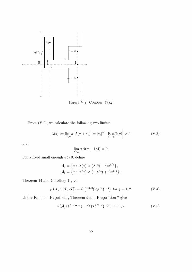
0 1

1 + iθ

1− iθ

14

s0

C (s0)

Figure V.2: Contour C (s0)

From (V.2), we calculate the following two limits:

λ(θ) := limσ0

σ|A(σ + s0)| = |s0|−1

∣∣∣∣Resη=s0D(η)

∣∣∣∣ > 0 (V.3)

andlimσ0

σA(σ + 1/4) = 0.

For a fixed small enough ε > 0, define

A1 =x : ∆(x) > (λ(θ)− ε)x1/4

,

A2 =x : ∆(x) < (−λ(θ) + ε)x1/4

.

Theorem 14 and Corollary 1 give

µ (Aj ∩ [T, 2T ]) = Ω(T 1/2(log T )−12

)for j = 1, 2. (V.4)

Under Riemann Hypothesis, Theorem 9 and Proposition 7 give

µ (Aj ∩ [T, 2T ]) = Ω(T 3/4−ε) for j = 1, 2. (V.5)

55

From Corollary 2, we get∫Aj∩[T,2T ]

∆2(x)dx = Ω(T 3/2

)for j = 1, 2. (V.6)

4 An Omega Theorem

Recall that (see Theorem 14)∑n≤x

|τ(n, θ)|2 =M(x) + ∆(x),

where the main term

M(x) = ω1(θ)x log x+ ω2(θ)x cos(θ log x) + ω3(θ)x

comes from the poles of D(s) at s = 1, 1 + iθ and s = 1− iθ. We may observe fromCorollary 2 that if D(s) has a complex pole at s0 = σ0 + it0, other than 1 + iθ and1− iθ, then ∫ 2T

T

∆(x)dx = Ω(x2σ0+1).

By Riemann Hypothesis, the only positive value for σ0 is 14, which is same as (V.6).

In this section, we shall use a technique due to Balasubramanian, Ramachandra andSubbarao [5] to improve this omega bound further. Now we state the main theoremof this section.

Theorem 15. For any c > 0 and for a sufficiently large T depending on c, we get∫ ∞T

|∆(x)|2

x2α+1e−2x/yduc exp

(c(log T )7/8

), (V.7)

whereα = α(T ) =

3

8− c

(log T )1/8.

In particular, this implies

∆(x) = Ω(x3/8 exp(−c(log x)7/8),

for some suitable c > 0.In order to prove the theorem, we need several lemmas, which form the content

of this section. We begin with a fixed δ0 ∈ (0, 1/16] for which we would choose anumerical value at the end of this section.

56

Definition 10. For T > 1, let Z(T ) be the set of all γ such that

1. T ≤ γ ≤ 2T ,

2. either ζ(β1 + iγ) = 0 for some β1 ≥ 12

+ δ0

or ζ(β2 + i2γ) = 0 for some β2 ≥ 12

+ δ0.

LetIγ,k = T ≤ t ≤ 2T : |t− γ| ≤ k log2 T for k = 1, 2.

We finally defineJk(T ) = [T, 2T ] \ ∪γ∈Z(T )Iγ,k.

Lemma 8. With the above definition, we have for k = 1, 2

µ(Jk(T )) = T +O(T 1−δ0/4 log3 T

).

Proof. We shall use an estimate on the function N(σ, T ), which is defined as

N(σ, T ) := |σ′ + it : σ′ ≥ σ, 0 < t ≤ T, ζ(σ′ + it) = 0| .

Selberg [38, Page 237] proved that

N(σ, T ) T 1− 14

(σ− 12

) log T, for σ > 1/2.

Now the lemma follows from the above upper bound on N(σ, t), and the observationthat

| ∪γ∈Z(T ) Iγ,k| N

(1

2+ δ0, T

)log2 T.

The next lemma closely follows Theorem 14.2 of [38], but does not depend onRiemann Hypothesis.

Lemma 9. For t ∈ J1(T ) and σ = 1/2 + δ with δ0 < δ < 1/4− δ0/2, we have

|ζ(σ + it)|±1 exp

(log log t

(log t

δ0

) 1−2δ1−2δ0

)

and

|ζ(σ + 2it)|±1 exp

(log log t

(log t

δ0

) 1−2δ1−2δ0

).

57

Proof. We provide a proof of the first statement, and the second statement can besimilarly proved.

Let 1 < σ′ ≤ log t. We consider two concentric circles centered at σ′ + it, withradius σ′− 1/2− δ0/2 and σ′− 1/2− δ0. Since t ∈ J1(T ) and the radius of the circleis log t, we conclude that

ζ(z) 6= 0 for |z − σ′ − it| ≤ σ′ − 1

2− δ0

2

and also ζ(z) has polynomial growth in this region. Thus on the larger circle,log |ζ(z)| ≤ c17 log t, for some constant c17 > 0. By Borel-Carathéodory theorem,

|z − σ′ − it| ≤ σ′ − 1

2− δ0 implies | log ζ(z)| ≤ c18σ

′

δ0

log t,

for some c18 > 0. Let 1/2 + δ0 < σ < 1, and ξ > 0 be such that 1 + ξ < σ′. Weconsider three concentric circles centered at σ′ + it with radius r1 = σ′ − 1 − ξ,r2 = σ′ − σ and r3 = σ′ − 1/2− δ0, and call them C1, C2 and C3 respectively. Let

Mi = supz∈Ci| log ζ(z)|.

From the above bound on | log ζ(z)|, we get

M3 ≤c18σ

′

δ0

log t.

Suitably enlarging c18, we see that

M1 ≤c18

ξ.

Hence we can apply the Hadamard’s three circle theorem to conclude that

M2 ≤M1−ν1 Mν

3 , for ν =log(r2/r1)

log(r3/r1).

Thus

M2 ≤(c18

ξ

)1−ν (c18σ

′ log t

δ0

)ν.

It is easy to see that

ν = 2− 2σ +4δ0(1− σ)

1 + 2ξ − 2δ0

+O(ξ) +O

(1

σ′

).

58

Now we put

ξ =1

σ′=

1

log log t.

HenceM2 ≤

c18 logν t log log t

δν0=c19 log log t

δν0(log t)

2−2σ+4δ0(1−σ)1+2ξ−2δ0 ,

for some c19 > 0. We observe that

2− 2σ +4δ0(1− σ)

1 + 2ξ − 2δ0

< 2− 2σ +4δ0(1− σ)

1− 2δ0

=1− 2δ

1− 2δ0

.

So we get

| log ζ(σ + it)| ≤ c19 log log t

(log t

δ0

) 1−2δ1−2δ0

,

and hence the lemma.

We put y = T b, for a constant b ≥ 8. Now suppose that∫ ∞T

|∆(u)|2

u2α+1e−u/ydu ≥ log2 T,

for sufficiently large T . Then clearly

∆(u) = Ω(uα).

Our next result explores the situation when such an inequality does not hold.

Proposition 5. Let δ0 < δ < 14− δ0

2. For 1/4 + δ/2 < α < 1/2, suppose that∫ ∞

T

|∆(u)|2

u2α+1e−u/ydu ≤ log2 T (V.8)

for any sufficiently large T . Then we have∫Re(s)=αt∈J2(T )

|D(s)|2

|s|2 1 +

∫ ∞T

|∆(u)|2

u2α+1e−2u/ydu.

Before embarking on a proof, we need the following technical lemmas.

Lemma 10. For 0 ≤ <(z) ≤ 1 and |Im(z)| ≥ log2 T , we have∫ ∞T

e−u/yu−zdu =T 1−z

1− z+O(T−b

′) (V.9)

59

and ∫ ∞T

e−u/yu−z log u du =T 1−z

1− zlog T +O(T−b

′), (V.10)

where b′ > 0 depends only on b.

Proof. By changing variable by v = u/y, we get∫ ∞T

e−u/y

uzdu = y1−z

∫ ∞T/y

e−vv−zdv.

Integrating the right hand side by parts∫ ∞T/y

e−vv−zdv =e−T/y

1− z

(T

y

)1−z

+1

1− z

∫ ∞T/y

e−vv1−zdv

It is easy to see that∫ ∞T/y

e−vv1−zdv = Γ(2− z) +O

((T

y

)2−Re(z)).

Hence (V.9) follows using e−T/y = 1 +O(T/y) and Stirling’s formula along with theassumption that |Im(z)| ≥ log2 T .

Proof of (V.10) proceeds in the same line and uses the fact that∫ ∞T/y

e−vv1−z log v dv = Γ′(2− z) +O

((T

y

)2−Re(z)

log T

).

Then we apply Stirling’s formula for Γ′(s) instead of Γ(s).

Lemma 11. Under the assumption (V.8), there exists T0 with T ≤ T0 ≤ 2T suchthat

∆(T0)e−T0/y

Tα0 log2 T,

and1

y

∫ ∞T0

∆(u)e−u/y

uαdu log T.

Proof. The assumption (V.8) implies that

log2 T ≥∫ 2T

T

|∆(u)|2

u2α+1e−u/ydu

=

∫ 2T

T

|∆(u)|2

u2αe−2u/y e

u/y

udu

60

≥ minT≤u≤2T

(|∆(u)|uα

e−u/y)2

,

which proves the first assertion. To prove the second assertion, we use the previousassertion and Cauchy- Schwartz inequality along with assumption (V.8) to get(∫ ∞

T0

|∆(u)|2

uαe−u/ydu

)2

≤(∫ ∞

T0

|∆(u)|2

u2α+1e−u/ydu

)(∫ ∞T0

ue−u/ydu

) y2 log2 T.

This completes the proof of this lemma.

We now recall a mean value theorem due to Montgomery and Vaughan [30].

Notation. For a real number θ, let ‖θ‖ := minn∈Z |θ − n|.

Theorem 16 (Montgomery and Vaughan [30]). Let a1, · · · , aN be arbitrary complexnumbers, and let λ1, · · · , λN be distinct real numbers such that

δ = minm,n‖λm − λn‖ > 0.

Then ∫ T

0

∣∣∣∣∣∑n≤N

an exp(iλnt)

∣∣∣∣∣2

dt =

(T +O

(1

δ

))∑n≤N

|an|2.

Lemma 12. For T ≤ T0 ≤ 2T and <(s) = α, we have

∫ 2T

T

∣∣∣∣∣∑n≤T0

|τ(n, θ)|2

nse−n/y

∣∣∣∣∣2

t−2dt 1.

Proof. Using theorem 16, we get∫ 2T

T

∣∣∣∣∣∑n≤T0

|τ(n, θ)|2

nse−n/y

∣∣∣∣∣2

t−2dt ≤ 1

T 2

(T∑n≤T0

|b(n)|2 +O

(∑n≤T0

n|b(n)|2))

,

where b(n) =|τ(n, θ)|2

nαe−n/y.

Thus∑n≤T0

|b(n)|2 ≤∑n≤T0

d(n)4

n2α T 1−2α+ε

0 and∑n≤T0

n|b(n)|2 ≤∑n≤T0

d(n)4

n2α−1 T 2−2α+ε

0

61

for any ε > 0, since the divisor function d(n) nε. As we have α > 0, this completesthe proof.

Lemma 13. For <(s) = α and T ≤ T0 ≤ 2T , we have

∫ 2T

T

∣∣∣∣∣∑n≥0

∫ 1

0

∆(n+ x+ T0)e−(n+x+T0)/y

(n+ x+ T0)s+1dx

∣∣∣∣∣2

dt∫ ∞T

|∆(x)|2

x2α+1e−2x/ydx.

Proof. Using Cauchy- Schwarz inequality, we get∣∣∣∣∣∑n≥0

∫ 1

0

∆(n+ x+ T0)

(n+ x+ T0)s+1e−(n+x+T0)/ydx

∣∣∣∣∣2

≤∫ 1

0

∣∣∣∣∣∑n≥0

∆(n+ x+ T0)

(n+ x+ T0)s+1e−(n+x+T0)/y

∣∣∣∣∣2

dx.

Hence ∫ 2T

T

∣∣∣∣∣∫ 1

0

∑n≥0

∆(n+ x+ T0)e−(n+x+T0)/y

(n+ x+ T0)s+1dx

∣∣∣∣∣2

dt

≤∫ 2T

T

∫ 1

0

∣∣∣∣∣∑n≥0

∆(n+ x+ T0)

(n+ x+ T0)s+1e−(n+x+T0)/y

∣∣∣∣∣2

dxdt

=

∫ 1

0

∫ 2T

T

∣∣∣∣∣∑n≥0

∆(n+ x+ T0)

(n+ x+ T0)s+1e−(n+x+T0)/y

∣∣∣∣∣2

dtdx.

From Theorem 16, we can get∫ 2T

T

∣∣∣∣∣∑n≥0

∆(n+ x+ T0)

(n+ x+ T0)s+1e−(n+x+T0)/y

∣∣∣∣∣2

dt

= T∑n≥0

|∆(n+ x+ T0)|2

(n+ x+ T0)2α+2e−2(n+x+T0)/y +O

(∑n≥0

|∆(n+ x+ T0)|2

(n+ x+ T0)2α+1

)

∑n≥0

|∆(n+ x+ T0)|2

(n+ x+ T0)2α+1e−2(n+x+T0)/y.

62

Hence ∫ 2T

T

∣∣∣∣∣∑n≥0

∫ 1

0

∆(n+ x+ T0)e−(n+x+T0)/T

(n+ x+ T0)s+1dx

∣∣∣∣∣2

dt

∫ 1

0

∑n≥0

|∆(n+ x+ T0)|2

(n+ x+ T0)2α+1e−2(n+x+T0)/ydx

∫ ∞T

|∆(x)|2

x2α+1e−2x/ydx,

completing the proof.

Proof of Proposition 5. For s = α+ it with 1/4+δ/2 < α < 1/2 and t ∈ J2(T ),we have

∞∑n=1

|τ(n, θ)|2

nse−n/y =

1

2πi

∫ 2+i∞

2−i∞D(s+ w)Γ(w)ywdw

=1

2πi

∫ 2+i log2 T

2−i log2 T

+O

(y2

∫ ∞log2 T

|D(s+ w)||Γ(w)|dw).

The above error term is estimated to be o(1). We move the integral to[1

4+δ

2− α− i log2 T,

1

4+δ

2− α + i log2 T

].

Let δ′ = 1/4 + δ/2 − α. In this region <(2s + 2w) = 1/2 + δ . So we can applyLemma 9 to conclude that D(s + w) = O(T κ), for some constant κ > 0. Thus theintegrals along horizontal lines are o(1). Since the only pole inside this contour is atw = 0, we get

∞∑n=1

|τ(n, θ)|2

nse−n/y = D(s) +

1

2πi

∫ δ′+i log2 T

δ′−i log2 T

D(s+ w)Γ(w)ywdw + o(1).

Since δ′ < 0, the remaining integral can be shown to be o(1) for b ≥ 8. Using T0 asin Lemma 11, we now divide the sum into two parts:

D(s) =∑n≤T0

|τ(n, θ)|2

nse−n/y +

∑n>T0

|τ(n, θ)|2

nse−n/y + o(1).

To estimate the second sum, we write

∑n>T0

|τ(n, θ)|2

nse−n/y =

∫ ∞T0

e−x/y

xsd

(∑n≤x

|τ(n, θ)|2)

63

=

∫ ∞T0

e−x/y

xsd(M(x) + ∆(x))

=

∫ ∞T0

e−x/y

xsM′(x)dx+

∫ ∞T0

e−x/y

xsd(∆(x)).

Recall thatM(x) = ω1(θ)x log x+ ω2(θ)x cos(θ log x) + ω3(θ)x,

thus

M′(x) = ω1(θ) log x+ ω2(θ) cos(θ log x)− θω2(θ) sin(θ log x) + ω1(θ) + ω3(θ).

Observe that∫ ∞T0

e−x/y

xscos(θ log x)dx =

1

2

∫ ∞T0

e−x/y

xs+iθdx+

1

2

∫ ∞T0

e−x/y

xs−iθdx.

Applying Lemma 10, we conclude that∫ ∞T0

e−x/y

xsM′(x)dx = o(1).

Integrating the second integral by parts:∫ ∞T0

e−x/y

xsd(∆(x)) =

e−T0/y∆(T0)

T s0

+1

y

∫ ∞T0

e−x/y

xs∆(x)dx− s

∫ ∞T0

e−x/y

xs+1∆(x)dx.

Applying Lemma 11, we get

∑n>T0

|τ(n, θ)|2

nse−n/y = s

∫ ∞T0

∆(x)e−x/y

xs+1dx+O(log T )

= s∑n≥0

∫ 1

0

∆(n+ x+ T0)e−(n+x+T0)/y

(n+ x+ T0)s+1dx+O(log T ).

Hence we have

D(s) =∑n≤T0

|τ(n, θ)|2

nse−n/y + s

∑n≥0

∫ 1

0

∆(n+ x+ T0)e−(n+x+T0)/y

(n+ x+ T0)s+1dx+O(log T ).

64

Squaring both sides, and then integrating on J2(T ), we get

∫J2(T )

|D(α + it)|2

|α + it|2dt

∫ 2T

T

∣∣∣∣∣∑n≤T0

|τ(n, θ)|2

nse−n/y

∣∣∣∣∣2

dt

t2

+

∫ 2T

T

∣∣∣∣∣∑n≥0

∫ 1

0

∆(n+ x+ T0)e−(n+x+T0)/y

(n+ x+ T0)s+1dx

∣∣∣∣∣2

dt.

The proposition now follows using Lemma 12 and Lemma 13.

We are now ready to prove our main theorem of this section.

Proof of Theorem 15. We prove by contradiction. Suppose that (V.7) does nothold. Then, given any N0 > 1, there exists T > N0 such that∫ ∞

T

|∆(x)|2

x2α+1e−2x/ydx exp

(c(log T )7/8

),

for all c > 0. This gives ∫ ∞T

|∆(x)|2

x2β+1e−2x/ydx 1,

whereβ =

3

8− c

2(log T )1/8.

We apply Proposition 5 to get∫J2(T )

|D(β + it)|2

|β + it|2dt 1. (V.11)

Now we compute a lower bound for the last integral over J2(T ). Write the functionalequation for ζ(s) as

ζ(s) = π1/2−sΓ((1− s)/2)

Γ(s/2)ζ(1− s).

Using the Stirling’s formula for Γ function, we get

|ζ(s)| = π1/2−βt1/2−β|ζ(1− s)|(

1 +O

(1

T

)),

65

for s = β + it. This implies

|D(β + it)| = t2−4β |ζ(1− β + it)2ζ(1− β − it− iθ)ζ(1− β − it+ iθ)||ζ(2β + i2t)|

.

Let δ0 = 1/16, and

β =3

8− c

2(log T )1/8=

1

2− δ

withδ =

1

8+

c

2(log T )1/8.

Then using Lemma 9, we get

|ζ(1− β + it)| =∣∣∣∣ζ (1

2+ δ + it

)∣∣∣∣ exp

(log log t

(log t

δ0

) 1−2δ1−2δ0

).

For t ∈ J2(T ) we observe that t ± θ ∈ J1(T ), and so the same bounds hold forζ(1− β + it+ iθ) and ζ(1− β + it− iθ). Further

|ζ(2β + i2t)| =∣∣∣∣ζ (1

2+

(1

2− 2δ

)+ i2t

)∣∣∣∣ exp

(log log t

(log t

δ0

) 4δ1−2δ0

).

Combining these bounds, we get

|D(β + it)| t2−4β exp

(−5 log log t

(log t

δ0

) 1−2δ1−2δ0

).

Therefore∫J2(T )

|D(β + it)|2dt ∫J2(T )

|D(β + it)|2dt∫J2(T )

|D(β + it)|2dt

T 4−8β exp

(−10 log log T

(log T

δ0

) 1−2δ1−2δ0

)µ(J2(T ))

T 5−8β exp

(−10 log log T

(log T

δ0

) 1−2δ1−2δ0

),

where we use Lemma 8 to show that µ(J2(T )) T . Now putting the values of δ

66

and δ0 as chosen above, we get∫J(T )

|D(β + it)|2

|β + it|2dt exp

(3c(log T )7/8

),

since 1−2δ1−2δ0

< 7/8. This contradicts (V.11), and hence the theorem follows.

The following two corollaries are immediate.

Corollary 3. For any c > 0 there exists an X-Set S, such that for sufficiently largeT depending on c there exists an

X ∈[T,T b

2log2 T

]∩ S,

for which we have ∫ 2X

X

|∆(x)|2

x2α+1dx ≥ exp

((c− ε)(logX)7/8

)with α as in Theorem 15 and for any ε > 0.

Corollary 4. For any c > 0 there exists an X-Set S, such that for sufficiently largeT depending on c there exists an

x ∈[T,T b

2log2 T

]∩ S,

for which we have∆(x) ≥ x3/8 exp

(−c(log x)7/8

).

We can now prove a "measure version" of the above result.

Proposition 6. For any c > 0, let

α(x) =3

8− c

(log x)1/8

and A = x : |∆(x)| xα(x). Then for every sufficiently large X depending on c,we have

µ(A ∩ [X, 2X]) = Ω(X2α(X)).

Proof. Suppose that the conclusion does not hold, hence

µ(A ∩ [X, 2X]) X2α(X).

67

Thus for every sufficiently large X, we get∫A∩[X,2X]

|∆(x)|2

x2α+1dx X2αM(X)

X2α+1=M(X)

X,

where α = α(X) and M(X) = supX≤x≤2X |∆(x)|2. Using dyadic partition, we canprove ∫

A∩[T,y]

|∆(x)|2

x2α+1dx M0(T )

Tlog T, where M0(T ) = sup

T≤x≤y|∆(x)|2

and y = T b for some b > 0 and T sufficiently large. This gives∫ ∞T

|∆(x)|2

x2α+1e−2x/ydx M0(T )

Tlog T.

Along with (V.7), this implies

M0(T ) T exp( c

2(log T )7/8

).

Thus|∆(x)| x

12 exp

( c4

(log x)7/8),

for some x ∈ [T, y]. This contradicts the fact that |∆(x)| x12 (log x)6.

4.1 Optimality of the Omega Bound

The following proposition shows the optimality of the omega bound in Corollary 3.

Proposition 7. Under Riemann Hypothesis (RH), we have∫ 2X

X

∆2(x)dx X7/4+ε,

for any ε > 0.

Proof. Theorem 2 (Perron’s formula) gives

∆(x) =1

2π

∫ T

−T

D(3/8 + it)x3/8+it

3/8 + itdt+O(xε),

for any ε > 0 and for T = X2 with x ∈ [X, 2X]. Using this expression for ∆(x), we

68

write its second moment as∫ 2X

X

∆2(x)dx =

∫ 2X

X

∫ T

−T

∫ T

−T

D(3/8 + it1)D(3/8 + it2)

(3/8 + it1)(3/8 + it2)x3/4+i(t1+t2)dx dt1dt2

+O(X1+ε(1 + |∆(x)|)

) X7/4

∫ T

−T

∫ T

−T

∣∣∣∣ D(3/8 + it1)D(3/8 + it2)

(3/8 + it1)(3/8 + it2)(7/4 + i(t1 + t2))

∣∣∣∣ dt1dt2 +O(X3/2+ε).

In the above calculation, we have used the fact that ∆(x) x12

+ε as in (I.4). Alsonote that for complex numbers a, b, we have |ab| ≤ 1

2(|a|2 + |b|2). We use this

inequality with

a =|D(3/8 + it1)|

|3/8 + it1|√|7/4 + i(t1 + t2)|

and b =|D(3/8 + it2)|

|3/8 + it2|√|7/4 + i(t1 + t2)|

,

to get∫ 2X

X

∆2(x)dx X7/4

∫ T

−T

∫ T

−T

∣∣∣∣D(3/8 + it2)

(3/8 + it2)

∣∣∣∣2 dt1|7/4 + i(t1 + t2)|

dt2 +O(X3/2+ε)

X7/4 logX

∫ T

−T

∣∣∣∣D(3/8 + it2)

(3/8 + it2)

∣∣∣∣2 dt2 +O(X3/2+ε).

Under RH, |D(3/8 + it2)| |t2|12

+ε. So we have∫ 2X

X

∆2(x)dx X7/4+ε for any ε > 0.

Note. The method we have used in Theorem 15 has its origin from the Plancherel’sformula in Fourier analysis. For instance, we may observe from Theorem 1 thatunder Riemann Hypothesis and other suitable conditions

∆(eu)

euσ=

1

2π

∫ ∞−∞

D(σ + it)eiut

σ + itdt for

1

4< σ ≤ 1

2.

So ∆(eu)euσ

is the Fourier transform of D(σ+it)σ+it

. By Plancherel’s formula∫ ∞−∞

|∆(eu)|e2uσ

du =1

4π2

∫ ∞−∞

∣∣∣∣D(σ + it)

σ + it

∣∣∣∣2 dt.

69

Now we change the variable u to log x and use the functional equation for ζ(s) toget ∫ ∞

1

∆2(x)

x2σ+1dx

∫ ∞1

∣∣∣∣D(σ + it)

σ + it

∣∣∣∣2 dt∫ ∞

1

t2−8σ−16ε

for any ε > 0. We may choose σ = 38− ε, then the above integral on the left side is

convergent. But if ∆(x) x38−ε, then the integral in the right diverges. This gives

∆(x) = Ω(x38−ε).

In [3] and [4], Balasubramanian and Ramachandra used this insight to obtain Ωbounds for the error terms in asymptotic formulas for partial sums of square-freedivisors and counting function for non-isomorphic abelian groups. This methodrequires the Riemann Hypothesis to be assumed in certain cases. Later Balasubra-manian, Ramachandra and Subbarao [5] modified this technique to apply on errorterm in the asymptotic formula for the counting function of k-full numbers with-out assuming Riemann Hypothesis. This method has been used by several authorsincluding [25] and [35].

5 Influence of Measure on Ω± Results

In this section, we shall show that for any ε > 0,

if ∆(x) x3/8+ε, then ∆(x) = Ω±(x3/8−ε) .

This improves our earlier result, which says that ∆(x) is Ω±(x1/4

). Now, we state

the main theorem of this section.

Theorem 17. Let ∆(x) be the error term of the summatory function of the twisteddivisor function as in Theorem 14. For c > 0, let

α(x) =3

8− c

(log x)1/8.

Let δ and δ′ be such that0 < δ < δ′ <

1

8.

Then either∆(x) = Ω

(xα(x)+ δ

2

)or ∆(x) = Ω±

(x

38−δ′).

To prove the above theorem, we estimate the growth of the Dirichlet series D(σ+ it)

70

by assuming that it does not have poles in a certain region.

Lemma 14. Let δ and σ be such that

0 < δ <1

8, and

3

8− δ ≤ σ <

1

2.

If D(σ + it) does not have a pole in the above mentioned range of σ, then for

3

8− δ +

δ

2(1 + log log(3 + |t|))< σ <

1

2,

we haveD(σ + it)δ,θ |t|2−2σ+ε

for any positive constant ε.

Proof. Let s = σ + it with 3/8− δ ≤ σ < 1/2. Recall that

D(s) =ζ2(s)ζ(s+ iθ)ζ(s− iθ)

ζ(2s).

Using functional equation, we write

D(s) = X (s)ζ2(1− s)ζ(1− s− iθ)ζ(1− s+ iθ)

ζ(2s), (V.12)

where X (s) is of order (can be obtained from Stirling’s formula for Γ)

X (σ + it) t2−4σ. (V.13)

Using Stirling’s formula and Phragmén-Lindelöf principle, we get

ζ(1− s)| |t|σ/2 log t.

So we get|ζ2(1− s)ζ(1− s− iθ)ζ(1− s+ iθ)| t2σ(log t)4. (V.14)

Now we shall compute an upper bound for |ζ(2s)|−1. This can be obtained in asimilar way as in Lemma 9. We choose t ≥ 100. Similar computation can be donewhen t is negative.

Consider two concentric circles C1,1 and C1,2, centered at 2 + it with radii

5

4+ 2δ and

5

4+ 2δ − δ

1 + log log(|t|+ 3).

71

The circle C1,1 passes through 3/4 − 2δ + i2t and C1,2 passes through 3/4 − 2δ +δ(1 + log log(|t| + 3))−1 + i2t. By our assumption, ζ(z) does not have any zero for|z−2− it| ≤ 5/4+2δ. This implies log ζ(z) is a holomorphic function in this region.It is easy to see that on the larger circle C1,1, we have log |ζ(z)| < σ′ log t for somepositive constant σ′. We apply Borel-Carathéodory theorem to get an upper boundfor log ζ(z) on C1,2 :

| log ζ(z)| ≤ 3δ−1(1 + log log(t+ 3)) (σ′ log t+ | log ζ(2 + it)|)≤ 10δ−1σ′(log log t) log t for z ∈ C1,2.

We may also note that if <(z − 3/4 − 2δ) > δ(log log t)−1 and =(z) ≤ t/2, thensimilar arguments give

| log ζ(z)| < δ−1σ′(log log t) log t,

for some positive constant σ′ that has changed appropriately.Now we consider three concentric circles C2,1, C2,2, C2,3, centered at σ′′ + i2t and

with radii r1 = σ′′ − 1− η, r2 = σ′′ − 2σ and r3 = σ′′ − δ0 respectively. Here

δ0 =3

4− 2δ +

δ

1 + log log(t+ 3).

We shall choose σ′′ = η−1 = log log t. Let M1,M2,M3 denote the supremums of| log ζ(z)| on C2,1, C2,2, C2,3 respectively. We have already calculated that

M3 ≤ δ−1σ′(log log t) log t.

It is easy to show thatM1 ≤ σ′ log log t,

where σ′ is again appropriately adjusted. Applying the three circle theorem weconclude

M2 ≤ σ′(log log t)δ−a loga t,

where

a =log(r2/r1)

log(r3/r1)=

1− 2σ + η

1− δ0 + η+O

(1

σ′′

)=

4(1− 2σ)

1 + 8δ+Oδ

(1

log log t

).

This gives|ζ(2s)|−1 exp

(c(log log t)(log t)

4(1−2σ)1+8δ

), (V.15)

72

for a suitable constant c > 0 depending on δ. The bound in the lemma follows from(V.12), (V.13), (V.14) and (V.15).

Now we complete the proof of Theorem 17.

Proof of Theorem 17. Let M be any large positive constant, and define

A := A(Mxα(x)).

Then from Corollary 3, we have∫[T,2T ]∩A

∆2(x)

x2α(T ) + 1dx exp

(c(log T )7/8

).

Assumingµ([T, 2T ] ∩ A) ≤ T 1−δ for T > T0, (V.16)

Proposition 3 gives∆(x) = Ω(xα(x)+δ/2)

as h0(T ) = T 1−δ, which is the first part of the theorem. But if (V.16) does not hold,then we have

µ([T, 2T ] ∩ A) > T 1−δ

for T in an X-Set . We choose

h1(T ) = T38− 2c

(log T )1/8−δ, α1(T ) =

3

8− 3c

(log T )1/8− δ, α2(T ) = α(T ).

Let δ′′ be such that δ < δ′′ < δ′. If D(σ + it) does not have pole for σ > 3/8 − δ′′then by Lemma 14, D(α1(T ) + it) has polynomial growth. So Assumptions 5 isvalid. Since

T 1−δ > 5h1(5T/2)T 1−α2(T ),

by case (ii) of Theorem 13 we have

∆(T ) = Ω±

(T

38− 3c

(log T )1/8−δ′′).

The second part of the above theorem follows from the choice δ′ > δ′′.

73

Bibliography

[1] R. J. Anderson and H. M. Stark. Oscillation theorems. In Analytic numbertheory (Philadelphia, Pa., 1980), volume 899 of Lecture Notes in Math., pages79–106. Springer, Berlin-New York, 1981.

[2] R. C. Baker. The square-free divisor problem. II. Quart. J. Math. Oxford Ser.(2), 47(186):133–146, 1996.

[3] R. Balasubramanian and K. Ramachandra. Effective and noneffective resultson certain arithmetical functions. J. Number Theory, 12(1):10–19, 1980.

[4] R. Balasubramanian and K. Ramachandra. Some problems of analytic numbertheory. III. Hardy-Ramanujan J., 4:13–40, 1981.

[5] R. Balasubramanian, K. Ramachandra, and M. V. Subbarao. On the errorfunction in the asymptotic formula for the counting function of k-full numbers.Acta Arith., 50(2):107–118, 1988.

[6] G. Bhowmik, J.-C. Schlage-Puchta, and O. Ramaré. Tauberian oscillation the-orems and the distribution of goldbach numbers. J. Théor. Nombres Bordeaux.To appear.

[7] K. Corrádi and I. Kátai. A comment on K. S. Gangadharan’s paper entitled“Two classical lattice point problems”. Magyar Tud. Akad. Mat. Fiz. Oszt.Közl., 17:89–97, 1967.

[8] A. Deitmar and S. Echterhoff. Principles of harmonic analysis. Universitext.Springer, New York, 2009.

[9] P. Èrdeš. An asymptotic inequality in the theory of numbers. Vestnik Leningrad.Univ., 15(13):41–49, 1960.

[10] K. Ford. The distribution of integers with a divisor in a given interval. Ann.of Math. (2), 168(2):367–433, 2008.

74

[11] K. Ford. Integers with a divisor in (y, 2y]. In Anatomy of integers, volume 46of CRM Proc. Lecture Notes, pages 65–80. Amer. Math. Soc., Providence, RI,2008.

[12] J. L. Hafner. New omega theorems for two classical lattice point problems.Invent. Math., 63(2):181–186, 1981.

[13] R. R. Hall and G. Tenenbaum. Divisors, volume 90 of Cambridge Tracts inMathematics. Cambridge University Press, Cambridge, 1988.

[14] G. H. Hardy. On Dirichlet’s Divisor Problem. Proc. London Math. Soc., S2-15(1):1–g.

[15] G. H. Hardy and J. E. Littlewood. Contributions to the theory of the rie-mann zeta-function and the theory of the distribution of primes. Acta Math.,41(1):119–196, 1916.

[16] G. H. Hardy and S. Ramanujan. The normal number of prime factors of anumber n [Quart. J. Math. 48 (1917), 76–92]. In Collected papers of SrinivasaRamanujan, pages 262–275. AMS Chelsea Publ., Providence, RI, 2000.

[17] G. H. Hardy and E. M. Wright. An introduction to the theory of numbers.Oxford University Press, Oxford, sixth edition, 2008. Revised by D. R. Heath-Brown and J. H. Silverman, With a foreword by Andrew Wiles.

[18] D. R. Heath-Brown. The number of abelian groups of order at most x.Astérisque, (198-200):153–163 (1992), 1991. Journées Arithmétiques, 1989 (Lu-miny, 1989).

[19] O. Hölder. Über einen asymptotischen Ausdruck. Acta Math., 59(1):89–97,1932.

[20] M. N. Huxley. Exponential sums and lattice points. III. Proc. London Math.Soc. (3), 87(3):591–609, 2003.

[21] A. Ivić. Large values of the error term in the divisor problem. Invent. Math.,71(3):513–520, 1983.

[22] A. Ivić. The number of finite nonisomorphic abelian groups in mean square.Hardy-Ramanujan J., 9:17–23, 1986.

[23] A. Ivić. The Riemann zeta-function. Dover Publications, Inc., Mineola, NY,2003. Theory and applications, Reprint of the 1985 original [Wiley, New York;MR0792089 (87d:11062)].

75

[24] J. Kaczorowski and B. Szydło. Some Ω-results related to the fourth powermoment of the Riemann zeta-function and to the additive divisor problem.9(1):41–50, 1997.

[25] M. Kühleitner and W. G. Nowak. On a question of A. Schinzel: Omega esti-mates for a special type of arithmetic functions. Cent. Eur. J. Math., 11(3):477–486, 2013.

[26] E. Landau. Über einen Satz von Tschebyschef. Math. Ann., 61(4):527–550,1906.

[27] K. Mahatab. Number of prime factors of an integer. Math. Newsl., 24(1):7–10,2013.

[28] K. Mahatab and A. Mukhopadhyay. Measure theoretic aspects of oscillationsof error terms. arXiv:1512.03144, 2016.

[29] K. Mahatab and K. Sampath. Chinese remainder theorem for cyclotomic poly-nomials in Z[X]. J. Algebra, 435:223–262, 2015.

[30] H. L. Montgomery and R. C. Vaughan. Hilbert’s inequality. J. London Math.Soc. (2), 8:73–82, 1974.

[31] Y. Motohashi. An explicit formula for the fourth power mean of the Riemannzeta-function. Acta Math., 170(2):181–220, 1993.

[32] Y. Motohashi. A relation between the Riemann zeta-function and the hyper-bolic Laplacian. Ann. Scuola Norm. Sup. Pisa Cl. Sci. (4), 22(2):299–313,1995.

[33] O. Robert and P. Sargos. Three-dimensional exponential sums with monomials.J. Reine Angew. Math., 591:1–20, 2006.

[34] R. E. Rodríguez, I. Kra, and J. P. Gilman. Complex analysis, volume 245 ofGraduate Texts in Mathematics. Springer, New York, second edition, 2013.

[35] A. Sankaranarayanan and K. Srinivas. On a method of Balasubramanian andRamachandra (on the abelian group problem). Rend. Sem. Mat. Univ. Padova,97:135–161, 1997.

[36] K. Soundararajan. Omega results for the divisor and circle problems. Int. Math.Res. Not., (36):1987–1998, 2003.

76

[37] G. Tenenbaum. Introduction to analytic and probabilistic number theory, vol-ume 46 of Cambridge Studies in Advanced Mathematics. Cambridge UniversityPress, Cambridge, 1995. Translated from the second French edition (1995) byC. B. Thomas.

[38] E. C. Titchmarsh. The theory of the Riemann zeta-function. The ClarendonPress, Oxford University Press, New York, second edition, 1986. Edited andwith a preface by D. R. Heath-Brown.

[39] K. M. Tsang. Higher-power moments of ∆(x), E(t) and P (x). Proc. LondonMath. Soc. (3), 65(1):65–84, 1992.

[40] H. von Koch. Sur la distribution des nombres premiers. Acta Math., 24(1):159–182, 1901.

77