measure of circularity for parts of digital boundaries and ... of circularity for parts of digital...
TRANSCRIPT

Measure of Circularity for Parts of Digital
Boundaries and its Fast Computation ?
Tristan Roussillon 1
Universite de Lyon,
Universite Lyon 2, LIRIS, UMR5205, F-69676, FRANCE
Isabelle Sivignon
Universite de Lyon, CNRS
Universite Lyon 1, LIRIS, UMR5205, F-69622, FRANCE
Laure Tougne
Universite de Lyon,
Universite Lyon 2, LIRIS, UMR5205, F-69676, FRANCE
Abstract
This paper focuses on the design of an effective method that computes the measure
of circularity of a part of a digital boundary. An existing circularity measure of a set
of discrete points, which is used in computational metrology, is extended to the case
of parts of digital boundaries. From a single digital boundary, two sets of points are
extracted so that the circularity measure computed from these sets is representative
of the circularity of the digital boundary. Therefore, the computation consists of two
steps. First, the inner and outer sets of points are extracted from the input part of
digital boundary using digital geometry tools. Next, the circularity measure of these
Preprint submitted to Elsevier 7 April 2009
sets is computed using classical tools of computational geometry. It is proved that
the algorithm is linear in time in the case of convex parts thanks to the specificity
of digital data, and is in O(n log n) otherwise. Experiments done on synthetic and
real images illustrate the interest of the properties of the circularity measure.
Key words: circularity, compactness, digital circle, discrete geometry,
computational geometry
1 Introduction1
Accurately locate circles and accurately measure deviation with a circular2
template are common problems in many fields of science and engineering. The3
fields of application are as diverse as geology [1], archeology [2], computer4
vision such as raster-to-vector conversion [3] or video processing [4], compu-5
tational metrology to test the quality of manufactured parts [5–12], image6
processing and discrete geometry to recognize digital circles [13–20].7
This paper focuses on the design of an effective method that computes the8
measure of circularity of a part of a digital boundary previously extracted9
from a digital image. The circularity measure of a given part of a digital10
boundary is a quantity that increases with deviation from a piece of digital11
circle, called a digital arc. The reader may find in the literature terms as diverse12
as compactness [21,13], roundness [22,6,8–11], out-of-roundness [5,6,23], but13
we prefer “circularity” [24,7] because it recalls the template with which the14
data are compared to, that is the circle.15
? Work partially supported by the GEODIB ANR project (ANR-06-BLAN-0225)Email address: [email protected] (Tristan Roussillon).
1 Author supported by a grant from the DGA
2

Although plenty of papers present methods for assessing the circularity of a set16
of points, as far as we know, only one paper dealt with the circularity of digital17
boundaries, more than twenty years ago. In [13], a digital disk recognition18
algorithm in O(n2) is presented in the first part, and a digital compactness19
evaluation algorithm for digital convex objects in O(n3√n) is presented in20
the second part (where n is the number of pixels of the digital boundary).21
The digital compactness measure is defined as the ratio between area A of the22
shape and area A′ of the smallest enclosing digital disk (where “the smallest”23
is expressed in area unit, that is in number of pixels). As a smallest enclosing24
digital disk may not be unique and as the smallest enclosing euclidean disk25
may not be a smallest enclosing digital disk, areas of many digital disks have26
to be compared. This is why the computational cost is rather high. This first27
attempt shows that the problem is not trivial.28
Moreover, naive methods that consist to find an easy-to-compute point that is29
expected to be the centre of a circle separating the shape from the background30
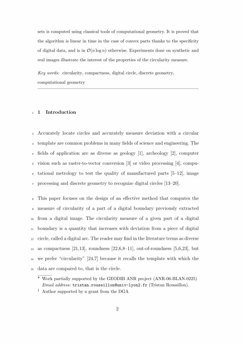
are only approximative. For instance, in [25], the barycentre of a set of pixels31
is assumed to be the centre of a separating circle, but Fig. 1 shows that if the32
barycentre of a set of pixels is computed, pixels that do not belong to the set33
may be closer to the barycentre than pixels that belong to the set, even if it34
turns out that the set of pixels can be separated from the pixels that do not35
belong to the set.36
A well-known circularity measure in the Euclidean plane is 4πA/P 2 where A37
is the area and P the perimeter. The digital equivalent of this circularity mea-38
sure was introduced by [21], but even with a convergent perimeter estimation39
based on digital straight segment recognition (see [26] and [27]) the measure is40
theoretically unsatisfactory: digital circles may have different values that are41
3
3.2
3.2
2.8 2.73 3 3.55
2.42 2.861.85 1.73 2.14
2.4 3.37
3.71
4.363.83
2.8 1.85 1 0.77 1.47
2.31
2.63
3.24
4.01 4.65
4.01
3.53
3.32.73
3
3.55
4.26
1.73
2.14
0.77 1.320.41
1.47 1.32 1.82
2.86 2.4 2.31 2.63
3.71 3.37 3.3 3.53
Fig. 1. A digital disk is depicted with pixels. In each pixel, the distance of its centre
to the barycentre of the digital disk (located with a cross) is written. Some pixels
that do not belong to the disk are closer (3.2) to the barycentre than some pixels
that belong to the disk (3.24)
always strictly less than 1. Moreover, this kind of measure has several other42
drawbacks in practice: (i) it is not perfectly scale invariant, (ii) it is not easy43
to interpret (iii) it is not computable on parts of a digital boundary and (iv) it44
is not able to provide the parameters of a circle that is close to the data. This45
measure may be used for a coarse and quick approximation of the circularity46
of a digital boundary, but in the general case, another measure is needed.47
Three kinds of methods may be found is the literature:48
(1) Methods based on the circular Hough transform [28–30] allow extraction,49
detection and recognition of digital arcs. Even if these methods are ro-50
bust against shape distortions, noise and occlusions, they require massive51
computations and memory, and thresholds tuning. As the digital bound-52
ary is assumed to be extracted from the digital image in this paper, the53
following methods are more appropriate.54
(2) Methods based on the separating circle problem in discrete and com-55
4
putational geometry [14–20] allow the recognition of digital arcs. These56
algorithms are not robust since one point can forbid the recognition of57
a digital arc. They need to be modified to measure the extent of the58
deviation with a digital arc.59
(3) Methods based on circle fitting are widely used. In computer vision [31–60
33,10,3,4], a circle is fitted to a set of pixels with the least square norm.61
In computational metrology [5,22,6,7,23,12], a circle is fitted to a set of62
points sampled on the boundary of a manufactured part by a Coordinate63
Measurement Machine (CMM) generally with the least L∞ norm (or64
Chebyshev or MinMax norm) because it is recommended by the American65
National Standards Institute (ANSI standard, B89.3.1-1972, R2002), but66
sometimes with the least square norm, like in [34].67
In this paper, a preliminary work presented in [35] is extended. Given a part68
of a digital boundary, the objective is to compute a circularity measure ful-69
filling some properties that will be enumerated in Section 2.2, as well as the70
parameters of one separating circle if it is a digital arc or the parameters of71
the closest circle otherwise. The proposed method is original because it is ap-72
plied on digital boundaries like in [13] and it links both methods based on the73
separating circle problem and methods based on circle fitting.74
We formally define a circularity measure for parts of digital boundaries in75
Section 2. From one digital boundary, two sets of points are extracted so that76
the circularity measure computed from these sets is representative of the cir-77
cularity of the digital boundary. Thanks to this trick, in spite of the specificity78
of the digital boundaries, an algorithm that only uses classical tools of com-79
putational geometry is derived in Section 3. Moreover, we show in Section 480
that the size of the two sets of points can be reduced in order to decrease the81
5

burden of the computation. Some experiments are done on synthetic digital82
boundaries and on real-word digital images in Section 5. The paper ends with83
some concluding words and future works in Section 6.84
2 Circularity measure for parts of digital boundary85
2.1 Data86
A binary image I is viewed as a subset of points of Z2 that are located inside87
a rectangle of size M×N . A digital object O ∈ I is a 4-connected subset of Z288
without any hole (Fig. 2.a). Its complementary set O = I\O is the so-called89
background. The digital boundary C (resp. C) of O (resp. O) is defined as the90
8-connected list of digital points having at least one 4-neighbour in O (resp.91
O) (Fig. 2.b). Without loss of generality, let us suppose that C is clockwise92
oriented. Each point of C is numbered according to its position in the list. The93
starting point, which is arbitrarily chosen, is denoted by C0. The last point is94
denoted by Cn−1, where n is equal to the number of points in C. A connected95
part Cij of C is the list of digital points from the i-th point to the j-th point96
of C (Fig. 2.c).97
A digital disk is defined as a digital object whose points are separable from the98
background by an Euclidean circle [13] (Fig. 2.d). A digital circle is defined as99
the boundary of a digital disk (Fig. 2.e) and a connected part of it is defined100
as a digital arc (Fig. 2.f).101
The goal of the following subsection is to define a measure of how much a102
given part of digital boundary is far from a digital arc.103
6
(a) (b) (c)
(d) (e) (f)
Fig. 2. (a) A digital object is depicted with black disks. The set of squares depicts
the whole (b) or a part of the (c) digital boundary. (d) A digital object that is a
digital disk. (e) A digital boundary that is a digital circle. (f) A part of a digital
boundary that is a digital arc.
2.2 Circularity measure of a part of a digital boundary104
A circularity measure for parts of digital boundaries is naturally expected to105
fulfil the following properties:106
(1) be robust to translation, rotation, scaling.107
(2) range from 0 to 1, equal 1 for a digital arc.108
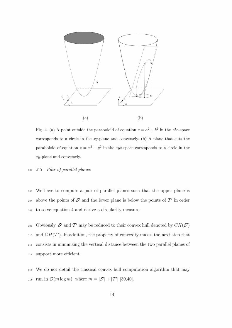
(3) be intuitive. For instance, it is naturally expected to increase as the num-109
ber of sides of regular polygons increases or as the eccentricity of ellipses110
7

m,l least square norm Chebyshev norm
radial mean square error minimum width annulus
distances [31,33,34] [5,22,6,7,9,10,12]
areal modified mean square error minimum area annulus
distances [32] [5,23]
Table 1
Some references for the four most used instances of the problem of fitting a circle
to a set of points
decreases or as the amount of noise decreases. It is also expected that the111
measure is robust: for example, the measure of a noisy digital circle has112
to be higher than the measure of a digital triangle or a digital square, if113
the noise is limited and does not affect the form.114
In metrology, the circularity of an arbitrary set of points in the plane is defined115
from the minimum cost of fitting a circle to the set given a certain norm. The116
most often used norm is either L2 (least square norm) or L∞ (MinMax or117
Chebyshev norm). Moreover, for both norms, the quantity that is minimized118
is either the sum of the radial distances or the sum of the areal distances. The119
four instances of the problem of fitting a circle to a set of points have been120
thoroughly studied for a long time as it is shown in Table 1.121
Fitting a circle to the points of a digital boundary with any of the above122
techniques does not lead to a satisfactory measure, because the property 2123
does not hold.124
8

(a) (b)
Fig. 3. Two parts of two digital boundaries are depicted with gray squares. S (resp.
T ) is the set of black disks (resp. white disks). In (a), the minimum area annulus
has an area of 4 and the circularity measure equals 8.5/12.5 = 0.68. However in (b),
it has a null area and the circularity measure equals 1, because the part of digital
boundary is a digital arc.
Our strategy may be coasely described as follows: from one digital boundary,125
two sets of points are extracted so that the circularity measure computed126
from these sets is representative of the circularity of the digital boundary.127
In the aim of fulfilling property 2, the circularity measure of these two sets128
is computed from the minimum signed area annulus such that the outer disk129
contains all the points of the digital object and the inner disk does not contain130
any background point (Fig. 3).131
Let S be the set of points of C and let T be the set of points of C. Let the132
minimum signed area annulus A of centre ω, inner radius r1 and outer radius133
r2 be such that the outer disk contains all the points of S and the inner disk134
does not contain any point of T :135
9
Find A that minimizes (r22 − r1
2)
subject to∀S ∈ S, (Sx − ωx)2 + (Sy − ωy)2 ≤ r2
2
∀T ∈ T , (Tx − ωx)2 + (Ty − ωy)2 > r12
(1)
Notice that the problem of finding a minimum signed area annulus enclosing a136
first set of points but not a second set of points is more general than, but may137
be reduced to the usual problem of finding a minimum area annulus enclosing138
a set of points (right bottom case of Table 1).139
The circularity measure of S and T is the squared ratio between r1 and r2:140
circ(S, T ) =r1
2
r22(2)
Now, we define the circularity measure of C as the circularity measure of S141
and T :142
circ(C) = circ(S, T ) if (circ(S, T ) < 1)
circ(C) = 1 otherwise
(3)
If the signed area π(r22−r1
2) of A is stricly less than 0, S and T are separable143
by a circle and circ(S, T ) > 1 but if π(r22 − r1
2) ≥ 0, S and T are not144
separable by a circle and circ(S, T ) ≤ 1. As a consequence the circularity145
measure defined in equation 3 fulfils property 2. Moreover, it is clear that the146
10
measure is also intuitive and is robust to rigid transformations, that is it fulfils147
properties 1 and 3.148
3 Computation of circ(S, T )149
This section focuses on the computation of circ(S, T ). First, we show that150
this computation may be achieved by linear programming in a space of di-151
mension 4. Next, we derive a simple geometric algorithm working in a space152
of dimension 3 only.153
3.1 Linear programming problem154
Developing the set of constraints of equation 1, we get:155
∀S ∈ S,−2aSx − 2bSy + f(Sx, Sy) + c2 ≤ 0
∀T ∈ T ,−2aTx − 2bTy + f(Tx, Ty) + c1 > 0
where
a = ωx, b = ωy,
c1 = (a2 + b2 − r12) c2 = (a2 + b2 − r2
2)
f(x, y) = x2 + y2
(4)
Instead of characterizing a circle by its centre and its radius, we characterize156
a circle by its centre and the power of the origin with respect to the circle.157
Thanks to this change of variables, solving equation 1 is equivalent to solving a158
linear program with four variables and |S|+ |T | constraints (where |.| denotes159
11
the cardinality of a set).160
This kind of reformulation into a linear programming problem has been done,161
for instance, in computational geometry for the smallest enclosing circle [36]162
or the smallest separating circle [14], in discrete geometry for digital circle163
recognition [19] and in engineering for the quality control of manufactured164
parts [23].165
The technique of Megiddo [37] is linear in time in the number of constraints.166
Unfortunately, Megiddo’s algorithm is not easy to implement and the constant167
is large and is exponential in the dimension, which is equal to 4 here. In a space168
of dimension 4, Megiddo’s algorithm cannot be used in practice. That’s why169
we propose in this section a simple geometric algorithm that works in a space170
of dimension 3 only.171
As an annulus is a pair of concentric circles that are characterized by three172
parameters each, we interpret equation 4 in a 3D space that we call abc-173
space. Indeed, c1 and c2, having the same meaning, are both represented in174
the c-axis. From now on, in addition to the original plane, called xy-plane,175
containing the points of Z2, we work in the abc-space as well as in its dual176
space, called xyz -space.177
3.2 abc-space vs xyz-space178
As 0 ≤ r1 ≤ r2, a2 + b2 ≤ c, the abc-space is a copy of R3 from which the179
interior of the paraboloid of equation c = a2 + b2 has been excluded. A point180
on the paraboloid maps to a circle of null radius in the xy-plane. A point that181
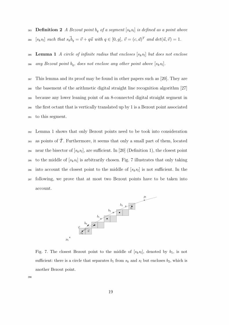
is out of the paraboloid maps to a circle whose radius is equal to the vertical182
12
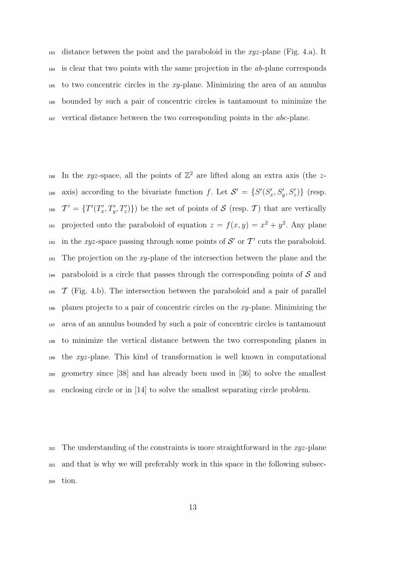
distance between the point and the paraboloid in the xyz -plane (Fig. 4.a). It183
is clear that two points with the same projection in the ab-plane corresponds184
to two concentric circles in the xy-plane. Minimizing the area of an annulus185
bounded by such a pair of concentric circles is tantamount to minimize the186
vertical distance between the two corresponding points in the abc-plane.187
In the xyz -space, all the points of Z2 are lifted along an extra axis (the z-188
axis) according to the bivariate function f . Let S ′ = {S ′(S ′x, S ′y, S ′z)} (resp.189
T ′ = {T ′(T ′x, T ′y, T ′z)}) be the set of points of S (resp. T ) that are vertically190
projected onto the paraboloid of equation z = f(x, y) = x2 + y2. Any plane191
in the xyz -space passing through some points of S ′ or T ′ cuts the paraboloid.192
The projection on the xy-plane of the intersection between the plane and the193
paraboloid is a circle that passes through the corresponding points of S and194
T (Fig. 4.b). The intersection between the paraboloid and a pair of parallel195
planes projects to a pair of concentric circles on the xy-plane. Minimizing the196
area of an annulus bounded by such a pair of concentric circles is tantamount197
to minimize the vertical distance between the two corresponding planes in198
the xyz -plane. This kind of transformation is well known in computational199
geometry since [38] and has already been used in [36] to solve the smallest200
enclosing circle or in [14] to solve the smallest separating circle problem.201
The understanding of the constraints is more straightforward in the xyz -plane202
and that is why we will preferably work in this space in the following subsec-203
tion.204
13
a
bc
(a)
x
yz
(b)
Fig. 4. (a) A point outside the paraboloid of equation c = a2 + b2 in the abc-space
corresponds to a circle in the xy-plane and conversely. (b) A plane that cuts the
paraboloid of equation z = x2 + y2 in the xyz -space corresponds to a circle in the
xy-plane and conversely.
3.3 Pair of parallel planes205
We have to compute a pair of parallel planes such that the upper plane is206
above the points of S ′ and the lower plane is below the points of T ′ in order207
to solve equation 4 and derive a circularity measure.208
Obviously, S ′ and T ′ may be reduced to their convex hull denoted by CH(S ′)209
and CH(T ′). In addition, the property of convexity makes the next step that210
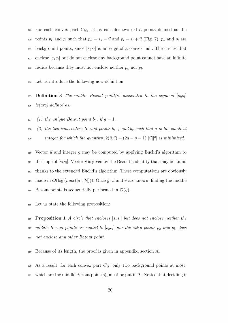
consists in minimizing the vertical distance between the two parallel planes of211
support more efficient.212
We do not detail the classical convex hull computation algorithm that may213
run in O(m logm), where m = |S ′|+ |T ′| [39,40].214
14
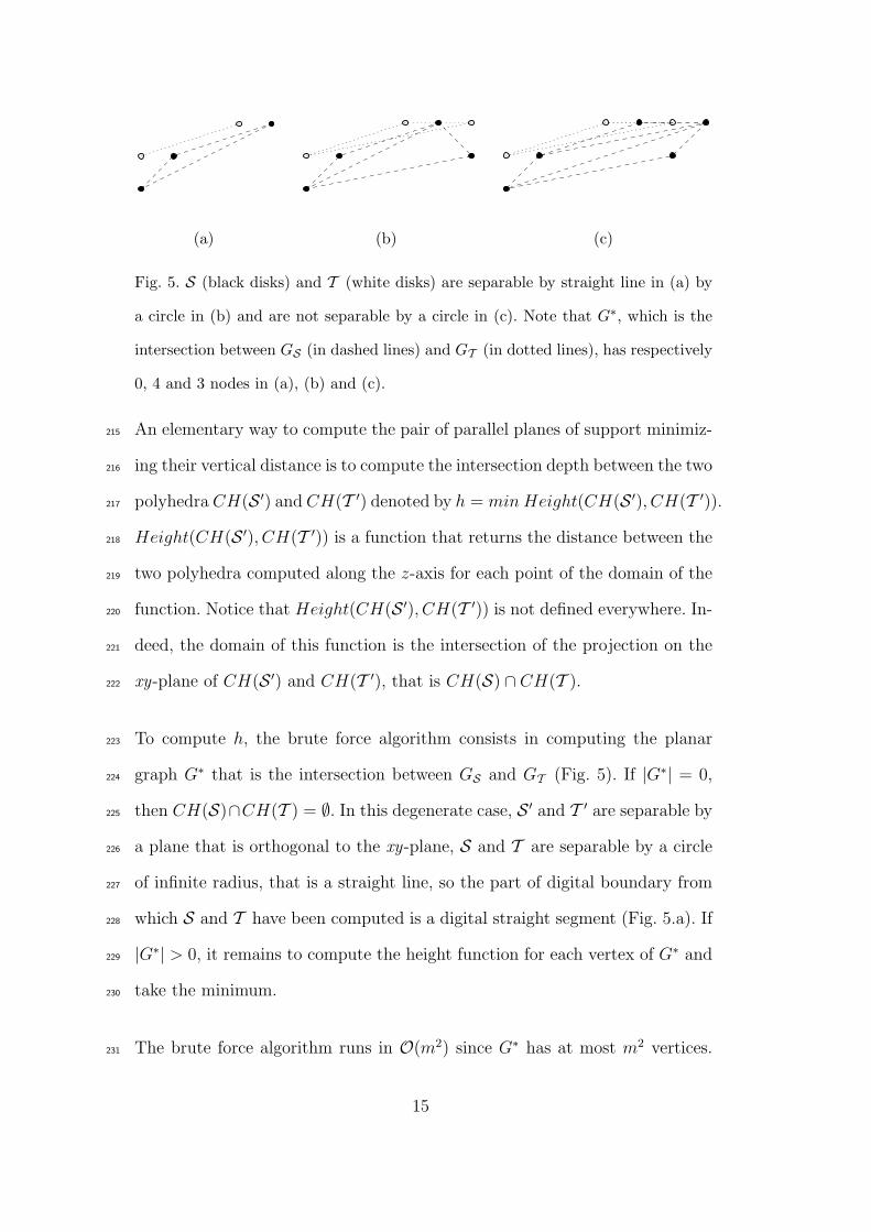
(a) (b) (c)
Fig. 5. S (black disks) and T (white disks) are separable by straight line in (a) by
a circle in (b) and are not separable by a circle in (c). Note that G∗, which is the
intersection between GS (in dashed lines) and GT (in dotted lines), has respectively
0, 4 and 3 nodes in (a), (b) and (c).
An elementary way to compute the pair of parallel planes of support minimiz-215
ing their vertical distance is to compute the intersection depth between the two216
polyhedra CH(S ′) and CH(T ′) denoted by h = min Height(CH(S ′), CH(T ′)).217
Height(CH(S ′), CH(T ′)) is a function that returns the distance between the218
two polyhedra computed along the z-axis for each point of the domain of the219
function. Notice that Height(CH(S ′), CH(T ′)) is not defined everywhere. In-220
deed, the domain of this function is the intersection of the projection on the221
xy-plane of CH(S ′) and CH(T ′), that is CH(S) ∩ CH(T ).222
To compute h, the brute force algorithm consists in computing the planar223
graph G∗ that is the intersection between GS and GT (Fig. 5). If |G∗| = 0,224
then CH(S)∩CH(T ) = ∅. In this degenerate case, S ′ and T ′ are separable by225
a plane that is orthogonal to the xy-plane, S and T are separable by a circle226
of infinite radius, that is a straight line, so the part of digital boundary from227
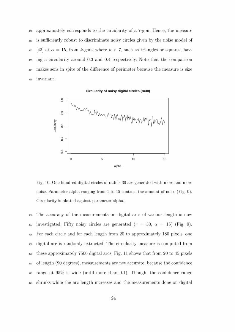
which S and T have been computed is a digital straight segment (Fig. 5.a). If228
|G∗| > 0, it remains to compute the height function for each vertex of G∗ and229
take the minimum.230
The brute force algorithm runs in O(m2) since G∗ has at most m2 vertices.231
15

However, it is possible to take advantage of the convexity of the height function232
to get an algorithm in O(m logm) (see [39, pages 310-315] for this algorithm).233
Although our algorithm is more general than a simple digital circle test, its234
complexity in O(m logm) is better than the quadratic complexity of the meth-235
ods presented in [15,16,20]. These methods cannot be efficient because they236
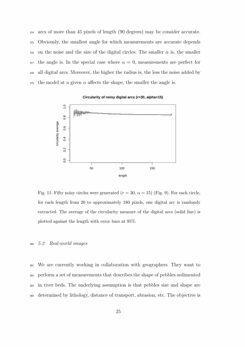
only deal with 2D projections of 3D polyhedrons.237
Once the pair of parallel planes of support are known, circ(S, T ) = r12
r22 , where238
r12 and r2
2 are derived from the coefficients of the pair of parallel planes. From239
equation 4, it is obvious to get the following equations: r12 = a2 + b2− c1 and240
r22 = a2 + b2 − c2.241
Since h is the signed area of the annulus A, if h < 0, S and T are separable242
by a circle and circ(S, T ) > 1 but if h ≥ 0, S and T are not separable by243
a circle and circ(S, T ) ≤ 1. Moreover, according to Lemma 1, Proposition 1244
and the definition of S and T given in Section 4, a part Cij of the digital245
boundary C is a digital arc if and only if S and T are separable by a circle.246
Hence, property 2 of Section 2.2 holds.247
Algorithm 1 sums up the current section.248
4 Minimization of the size of S and T249
In the aim of decreasing the burden of the computation of circ(S, T ), which250
depends on the size of S and T , we search for S and T such that S ∈ S,251
T ∈ T , |S|+ |T | < |S|+ |T | and circ(S, T ) = circ(S, T ).252
16
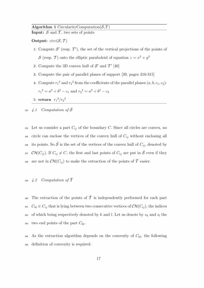
Algorithm 1 CircularityComputation(S,T )
Input: S and T , two sets of points
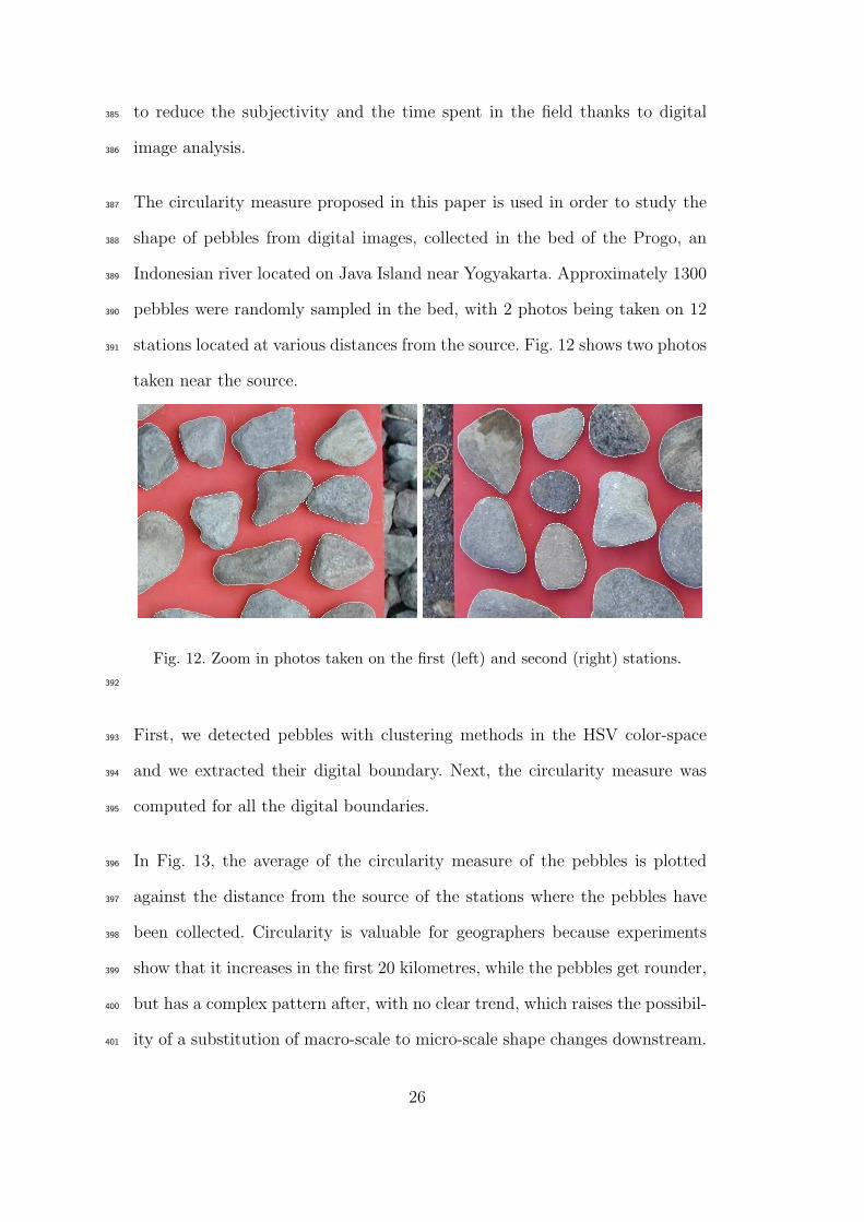
Output: circ(S, T )
1: Compute S ′ (resp. T ′), the set of the vertical projections of the points of
S (resp. T ) onto the elliptic paraboloid of equation z = x2 + y2
2: Compute the 3D convex hull of S ′ and T ′ [40]
3: Compute the pair of parallel planes of support [39, pages 310-315]
4: Compute r12 and r2
2 from the coefficients of the parallel planes (a, b, c1, c2):
r12 = a2 + b2 − c1 and r2
2 = a2 + b2 − c2
5: return r12/r2
2
4.1 Computation of S253
Let us consider a part Cij of the boundary C. Since all circles are convex, no254
circle can enclose the vertices of the convex hull of Cij without enclosing all255
its points. So S is the set of the vertices of the convex hull of Cij, denoted by256
CH(Cij). If Cij 6= C, the first and last points of Cij are put in S even if they257
are not in CH(Cij) to make the extraction of the points of T easier.258
4.2 Computation of T259
The extraction of the points of T is independently performed for each part260
Ckl ∈ Cij that is lying between two consecutive vertices of CH(Cij), the indices261
of which being respectively denoted by k and l. Let us denote by sk and sl the262
two end points of the part Ckl.263
As the extraction algorithm depends on the convexity of Ckl, the following264
definition of convexity is required:265
17
Definition 1 As Cij is clockwise oriented, the right (resp. left) part of CH(Cij)266
is the polygonal line that links Ci and Cj and that lies on the right (resp. left)267
of Cij. Cij is convex (resp. concave) if and only if there is no digital point268
between the polygonal line linking the digital points of Cij and the right (resp.269
left) part of CH(Cij).270
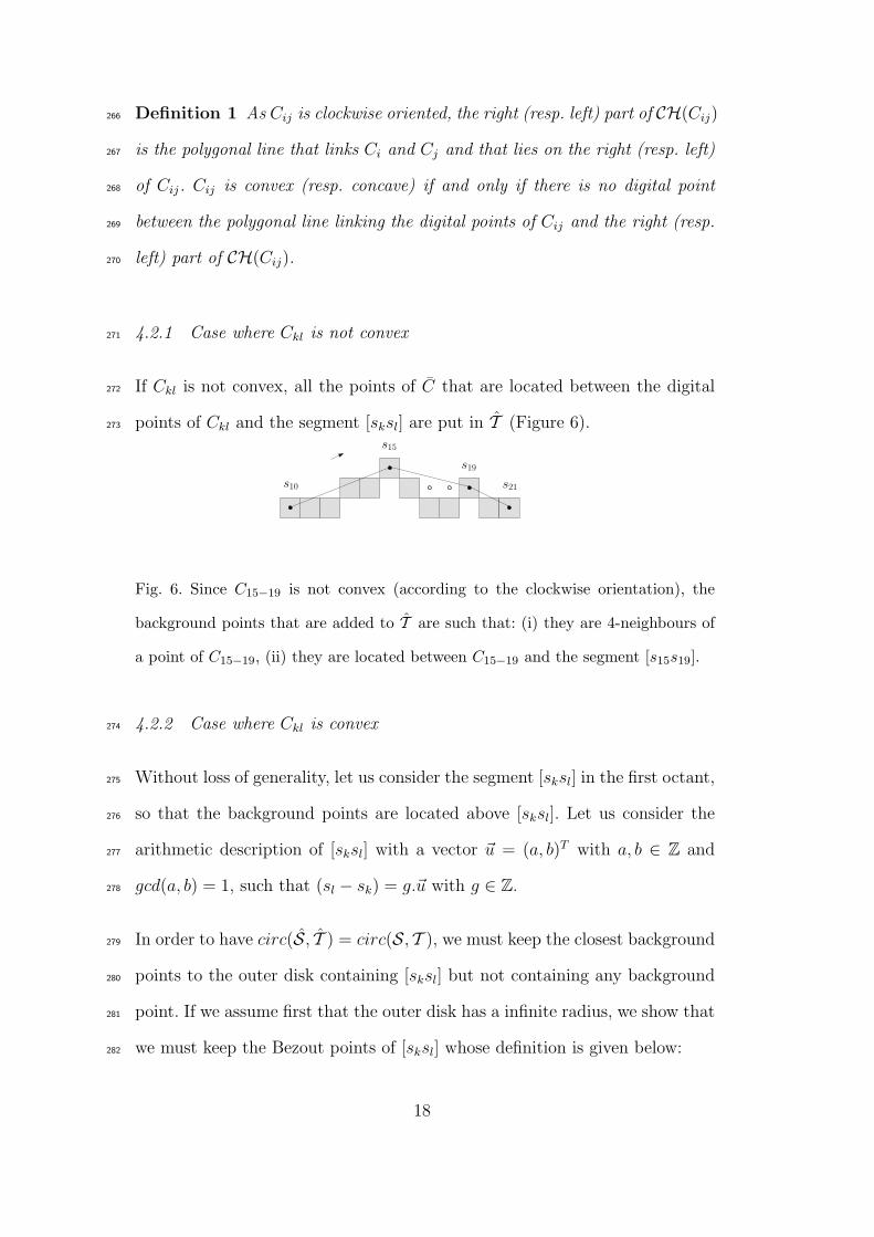
4.2.1 Case where Ckl is not convex271
If Ckl is not convex, all the points of C that are located between the digital272
points of Ckl and the segment [sksl] are put in T (Figure 6).273
s15
s10
s19
s21
Fig. 6. Since C15−19 is not convex (according to the clockwise orientation), the
background points that are added to T are such that: (i) they are 4-neighbours of
a point of C15−19, (ii) they are located between C15−19 and the segment [s15s19].
4.2.2 Case where Ckl is convex274
Without loss of generality, let us consider the segment [sksl] in the first octant,275
so that the background points are located above [sksl]. Let us consider the276
arithmetic description of [sksl] with a vector ~u = (a, b)T with a, b ∈ Z and277
gcd(a, b) = 1, such that (sl − sk) = g.~u with g ∈ Z.278
In order to have circ(S, T ) = circ(S, T ), we must keep the closest background279
points to the outer disk containing [sksl] but not containing any background280
point. If we assume first that the outer disk has a infinite radius, we show that281
we must keep the Bezout points of [sksl] whose definition is given below:282
18
Definition 2 A Bezout point bq of a segment [sksl] is defined as a point above283
[sksl] such that ~skbq = ~v + q~u with q ∈ [0, g], ~v = (c, d)T and det(~u,~v) = 1.284
Lemma 1 A circle of infinite radius that encloses [sksl] but does not enclose285
any Bezout point bq, does not enclose any other point above [sksl].286
This lemma and its proof may be found in other papers such as [20]. They are287
the basement of the arithmetic digital straight line recognition algorithm [27]288
because any lower leaning point of an 8-connected digital straight segment in289
the first octant that is vertically translated up by 1 is a Bezout point associated290
to this segment.291
Lemma 1 shows that only Bezout points need to be took into consideration292
as points of T . Furthermore, it seems that only a small part of them, located293
near the bisector of [sksl], are sufficient. In [20] (Definition 1), the closest point294
to the middle of [sksl] is arbitrarily chosen. Fig. 7 illustrates that only taking295
into account the closest point to the middle of [sksl] is not sufficient. In the296
following, we prove that at most two Bezout points have to be taken into297
account.
~v~u
sk
sl
pl
b0
b1
b2
b3
pk
Fig. 7. The closest Bezout point to the middle of [sksl], denoted by b1, is not
sufficient: there is a circle that separates b1 from sk and sl but encloses b2, which is
another Bezout point.
298
19
For each convex part Ckl, let us consider two extra points defined as the299
points pk and pl such that pk = sk − ~u and pl = sl + ~u (Fig. 7). pk and pl are300
background points, since [sksl] is an edge of a convex hull. The circles that301
enclose [sksl] but do not enclose any background point cannot have an infinite302
radius because they must not enclose neither pk nor pl.303
Let us introduce the following new definition:304
Definition 3 The middle Bezout point(s) associated to the segment [sksl]305
is(are) defined as:306
(1) the unique Bezout point b0, if g = 1.307
(2) the two consecutive Bezout points bq−1 and bq such that q is the smallest308
integer for which the quantity |2(~u.~v) + (2q − g − 1)||~u||2| is minimized.309
Vector ~u and integer g may be computed by applying Euclid’s algorithm to310
the slope of [sksl]. Vector ~v is given by the Bezout’s identity that may be found311
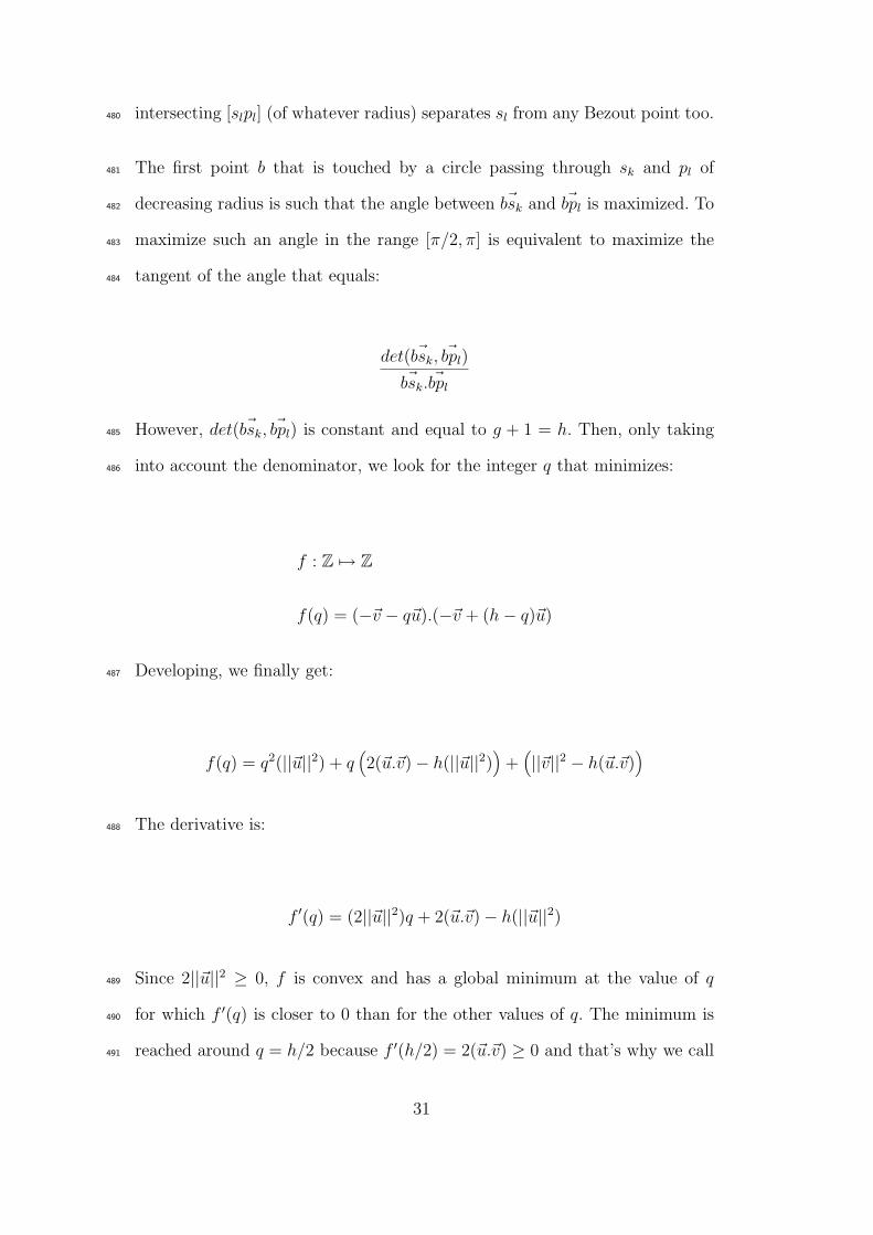
thanks to the extended Euclid’s algorithm. These computations are obviously312
made in O(log (max(|a|, |b|))). Once g, ~u and ~v are known, finding the middle313
Bezout points is sequentially performed in O(g).314
Let us state the following proposition:315
Proposition 1 A circle that encloses [sksl] but does not enclose neither the316
middle Bezout points associated to [sksl] nor the extra points pk and pl, does317
not enclose any other Bezout point.318
Because of its length, the proof is given in appendix, section A.319
As a result, for each convex part Ckl, only two background points at most,320
which are the middle Bezout point(s), must be put in T . Notice that deciding if321
20

the extra point pk (resp. pl) also must be added to T is done when considering,322
if it exists, the previous (resp. next) part of Cij. As an exception, if Ckl is the323
first (resp. last) convex part of Cij, then the extra point pk (resp. pl) is also324
added to T .325
4.3 Algorithm and Complexity326
The algorithm that computes S and T (Algorithm 2) is given below.327
Algorithm 2 SnTComputation(C,S and T )
Input: Cij, a part of a digital boundary
Output: S and T
1: S = T = ∅
2: Add si to S
3: Compute CH(Cij)
4: for each part Ckl of Cij do
5: Add sl to S
6: if Ckl is convex then
7: Add the middle Bezout point(s) of [sksl] to T
8: else
9: Add to T all the points of C that are located between the digital
points of Ckl and [sksl].
10: return S,T
Computing CH(Cij) (l.3) is done in linear time (using Melkman’s algorithm328
[42] for instance). All the background points that are 4-neighbours of a point329
of Ckl is computed in linear time by contour tracking. Checking whether each330
part Ckl is convex or not (l.6) and performing the appropriate processing (l.7331
21
and l.9) is then straightforward and in O(l − k).332
Fig. 8 illustrates that |S| and |T | are considerably smaller than |S| and |T |,333
if Cij is convex.334
(a) (b)
Fig. 8. S in (a) and S (b) (resp. T in (a) and T (b)) are depicted with black disks
(resp. white disks).
Actually, |S| is bounded by O(n2/3) according to known results [41]. If Cij is335
convex, |T | is at most twice bigger than |S| according to Proposition 1 and |T |336
is bounded by O(n) otherwise. Therefore m = |S|+ |T | is bounded by O(n2/3)337
in the case of convex parts and O(n) otherwise. As circ(S, T ) = circ(S, T )338
can be computed in O(m logm), we can conclude that the circularity measure339
of Cij can be computed in O(n) if Cij is convex and O(n log n) otherwise.340
5 Experiments341
It is clear that the proposed circularity measure fulfils the three properties of342
Section 2.2. In this section, the proposed circularity measure is probed with343
respect to its ability to deal with a part of a digital boundary.344
22

5.1 Synthetic images345
Hundreds of noisy circles are generated. In order to study the impact of the346
amount of noise onto circularity, we implemented a degradation model very347
close to the one investigated in [43]. This model was proposed and validated348
in the context of document analysis and assume that: (i) the probability to349
flip a pixel (that is, label ‘foreground’ or ‘1’ a pixel previously labelled ‘back-350
ground’ or ‘0’, and conversely) depends of its distance to the nearest pixel of351
the complement set and (ii) blurring may be simulated with a morphological352
closing.353
Figure 9 gives two examples of results of the degradation algorithm applied354
to a digital disk.355
r = 30, α = 1 r = 30, α = 15
Fig. 9. Gauss digitization of two disks. The amount of noise that is added to the
disks according to the degradation model of [43] depends of parameter alpha. The
digital curves that we are called upon to measure are the 8-connected boundaries
of these digital objects.
Figure 10 shows that the circularity decreases with the amount of noise, but356
with sawtooth because the pixels are flipped at random. The noisier the dig-357
ital circle, the more it looks different from a digital circle. Furthermore, even358
with rather noisy digital circles (α = 15), the circularity is above 0.8, which359
23
approximately corresponds to the circularity of a 7-gon. Hence, the measure360
is sufficiently robust to discriminate noisy circles given by the noise model of361
[43] at α = 15, from k-gons where k < 7, such as triangles or squares, hav-362
ing a circularity around 0.3 and 0.4 respectively. Note that the comparison363
makes sens in spite of the difference of perimeter because the measure is size364
invariant.365
0 5 10 15
0.6
0.7
0.8
0.9
1.0
alpha
Circ
ular
ity
Circularity of noisy digital circles (r=30)
Fig. 10. One hundred digital circles of radius 30 are generated with more and more
noise. Parameter alpha ranging from 1 to 15 controls the amount of noise (Fig. 9).
Circularity is plotted against parameter alpha.
The accuracy of the measurements on digital arcs of various length is now366
investigated. Fifty noisy circles are generated (r = 30, α = 15) (Fig. 9).367
For each circle and for each length from 20 to approximately 180 pixels, one368
digital arc is randomly extracted. The circularity measure is computed from369
these approximately 7500 digital arcs. Fig. 11 shows that from 20 to 45 pixels370
of length (90 degrees), measurements are not accurate, because the confidence371
range at 95% is wide (until more than 0.1). Though, the confidence range372
shrinks while the arc length increases and the measurements done on digital373
24
arcs of more than 45 pixels of length (90 degrees) may be consider accurate.374
Obviously, the smallest angle for which measurements are accurate depends375
on the noise and the size of the digital circles. The smaller α is, the smaller376
the angle is. In the special case where α = 0, measurements are perfect for377
all digital arcs. Moreover, the higher the radius is, the less the noise added by378
the model at a given α affects the shape, the smaller the angle is.379
50 100 150
0.0
0.2
0.4
0.6
0.8
1.0
length
circ
ular
ity a
vera
ge
Circularity of noisy digital arcs (r=30, alpha=15)
Fig. 11. Fifty noisy circles were generated (r = 30, α = 15) (Fig. 9). For each circle,
for each length from 20 to approximately 180 pixels, one digital arc is randomly
extracted. The average of the circularity measure of the digital arcs (solid line) is
plotted against the length with error bars at 95%.
5.2 Real-world images380
We are currently working in collaboration with geographers. They want to381
perform a set of measurements that describes the shape of pebbles sedimented382
in river beds. The underlying assumption is that pebbles size and shape are383
determined by lithology, distance of transport, abrasion, etc. The objective is384
25
to reduce the subjectivity and the time spent in the field thanks to digital385
image analysis.386
The circularity measure proposed in this paper is used in order to study the387
shape of pebbles from digital images, collected in the bed of the Progo, an388
Indonesian river located on Java Island near Yogyakarta. Approximately 1300389
pebbles were randomly sampled in the bed, with 2 photos being taken on 12390
stations located at various distances from the source. Fig. 12 shows two photos391
taken near the source.
Fig. 12. Zoom in photos taken on the first (left) and second (right) stations.392
First, we detected pebbles with clustering methods in the HSV color-space393
and we extracted their digital boundary. Next, the circularity measure was394
computed for all the digital boundaries.395
In Fig. 13, the average of the circularity measure of the pebbles is plotted396
against the distance from the source of the stations where the pebbles have397
been collected. Circularity is valuable for geographers because experiments398
show that it increases in the first 20 kilometres, while the pebbles get rounder,399
but has a complex pattern after, with no clear trend, which raises the possibil-400
ity of a substitution of macro-scale to micro-scale shape changes downstream.401
26

Notice that Fig. 12 shows photos taken on two stations that have statistically402
significant difference of circularity: the first station (Fig. 12, left) and the sec-403
ond one (Fig. 12, right). Obviously, other size, form and shape parameters,404
like diameter, elongation, convexity and roundness [1], are computed with cir-405
cularity to provide multidimensional data of great interest for geographers.406
0 10 20 30 40 50 60
0.40
0.45
0.50
0.55
0.60
distance from the source
circ
ular
ity a
vera
ge
Circularity of pebbles
Fig. 13. The average of the circularity measure of the pebbles is plotted against
the distance from the source of the 12 stations where the 1300 pebbles have been
collected.407
In the left photo of Fig. 12, two pebbles are badly detected because they touch408
each other. Another example is presented on the left of Fig. 14.409
In such cases, it is possible to cut the digital boundary in two and indepen-410
dently deal with the two parts of the digital boundary. We used an algorithm411
that robustly decomposes a digital curve into convex and concave parts [45].412
Each part may be viewed as a part of a pebble outline that has not been wholly413
retrieved. As the missing part of each outline is small enough, the circularity414
27

Fig. 14. Corrupted outlines of pebbles.
measure of the retrieved part is assumed to be very close to the one that could415
have been computed on the whole digital boundary. In the example presented416
in the left photo of Fig. 12, the circularity measure of the whole digital bound-417
ary is 0.005, whereas the circularity measure of the two parts corresponding418
to the two pebbles is 0.488 and 0.598 respectively, from left to right.419
In the right photo of Fig. 14, is presented a pebble outline that is corrupted420
with a spike. Using [45], the digital boundary is coarsely cut before and after421
the spike. The digital boundary with and without the spike has the same422
circularity measure that is equal to 0.511 because the spike does not affect the423
fitting of the minimum area annulus.424
Generally speaking, the proposed method is able to infer the circularity mea-425
sure of a digital boundary from a part of it, provided that bumps are uniformly426
spread around the boundary and that the part is long enough with respect427
to the amplitude of the bumps. For instance, in Section 5.1, it was shown428
that for circles of radius 30 that are corrupted by the noise model of [43] at429
α = 15, the measurements done on parts of more than 90 degrees may be430
consider accurate. We took profit of this property in our application to cope431
with occlusions and spikes.432
28
6 Conclusion and perspectives433
In this paper, a circularity measure has been defined for parts of digital bound-434
aries. An existing circularity measure of a set of discrete points, which is435
sometimes used in computational metrology, is extended to the case of parts436
of digital boundaries (Section 2.2). Once the minimum area annulus, such that437
the outer disk contains all the points of the part of a digital boundary and the438
inner disk does not contain any background point is computed, the circular-439
ity measure is defined as the squared ratio between the inner and outer radii440
(Section 2.2).441
Because we consider two sets of points, the problem we deal with is more442
general than the usual problem of finding a minimum area annulus enclosing443
one set of points [5,22,6,7,9,10,12]. The circularity measure of these two sets444
of points is computed thanks to an algorithm in O(n log n) that only uses445
classical tools of computational geometry (Section 3). Moreover, the two sets446
of points may be computed so that the algorithm is linear in time in the case447
of convex digital boundaries (Section 4). The method is exact contrary to448
many methods that use ad hoc heuristics [7] or meta-heuristics like simulated449
annealing [10,12]. Even if it is shown that a sophisticated machinery coming450
from linear programming can provide a linear time algorithm (Section 3.1),451
its time complexity is better than many quadratic methods based on Voronoi452
diagrams [15,16,5,22] (Section 3.3).453
Contrary to the famous measure introduced in [21], the measure proposed in454
this paper fulfils the following properties:455
• it may be applied on any part of digital boundaries.456
29

• it is robust to rigid transformations.457
• it ranges from 0 to 1 and is equal to 1 for any digital circle or arc, which458
means that the measurements are accurate even at low resolution.459
• it provides the parameters of a circle whose digitization is the measured460
part of digital boundary if the circularity measure is 1 and the parameters461
of an approximating circle otherwise.462
The kind of measure and algorithm proposed in this paper is general enough to463
be applied in order to recognize or measure the deviation with other quadratic464
shapes like parabolas. In the case of parabolas, the extension is straightfor-465
ward: it is enough to modify function f , so that f(x, y) equals x2 (or y2),466
instead of x2 + y2. The points of the xy-plane are merely vertically projected467
onto a parabolic cylinder instead of an elliptic paraboloid and algorithm 1468
does not change.469
To end, it would be quite valuable to make the algorithm on-line (without470
increasing its complexity as far as possible). The on-line property would be471
of great interest to efficiently and robustly decompose a digital boundary into472
primitives like noisy digital arcs or pieces of noisy digital parabolas.473
A Proof of Proposition 1474
In the sequel, we only consider the case of a circle that encloses [sksl] but nei-475
ther pl nor the closest middle Bezout point to pl. The other case is symmetric476
and the two cases will be put together to conclude the proof.477
Let us consider a circle passing through sk and pl. If such a circle encloses sl478
but does not enclose any Bezout point, then any circle passing through sk and479
30
intersecting [slpl] (of whatever radius) separates sl from any Bezout point too.480
The first point b that is touched by a circle passing through sk and pl of481
decreasing radius is such that the angle between ~bsk and ~bpl is maximized. To482
maximize such an angle in the range [π/2, π] is equivalent to maximize the483
tangent of the angle that equals:484
det( ~bsk, ~bpl)
~bsk. ~bpl
However, det( ~bsk, ~bpl) is constant and equal to g + 1 = h. Then, only taking485
into account the denominator, we look for the integer q that minimizes:486
f : Z 7→ Z
f(q) = (−~v − q~u).(−~v + (h− q)~u)
Developing, we finally get:487
f(q) = q2(||~u||2) + q(2(~u.~v)− h(||~u||2)
)+(||~v||2 − h(~u.~v)
)
The derivative is:488
f ′(q) = (2||~u||2)q + 2(~u.~v)− h(||~u||2)
Since 2||~u||2 ≥ 0, f is convex and has a global minimum at the value of q489
for which f ′(q) is closer to 0 than for the other values of q. The minimum is490
reached around q = h/2 because f ′(h/2) = 2(~u.~v) ≥ 0 and that’s why we call491
31

the Bezout point bq such that q is the smallest integer for which the quantity492
|2(~u.~v) + (2q − h)||~u||2| is minimized (Def. 3) the middle Bezout point.493
To end, the first point b that is touched by the circle of decreasing radius and494
passing through sk and pl is the closest middle Bezout point to pl according495
to Def. 3. Similarly, we can show that the first point b that is touched by the496
circle of decreasing radius and passing through sl and pk is the closest middle497
Bezout point to pk according to Def. 3, which concludes the proof. 2498
References
[1] H. Wadell, Volume, shape, and roundness of rock particles, Journal of Geology
40 (1932) 443–451.
[2] A. Thom, A statistical examination of megalithic sites in britain, Journal of
Royal Statistical Society 118 (1955) 275–295.
[3] X. Hilaire, K. Tombre, Robust and accurate vectorization of line drawings,
IEEE Transactions on Pattern Analysis and Machine Intelligence 28 (6) (2006)
890–904.
[4] I. Frosio, N. A. Borghese, Real-time accurate circle fitting with occlusions,
Pattern Recognition 41 (2008) 1045–1055.
[5] V.-B. Le, D. T. Lee, Out-of-roundness problem revisited, IEEE Transactions
on Pattern Analysis and Machine Intelligence 13 (3) (1991) 217–223.
[6] K. Swanson, D. T. Lee, V. L. Wu, An optimal algorithm for roundness
determination on convex polygons, Computational Geometry 5 (1995) 225–235.
[7] J. Pegna, C. Guo, Computational metrology of the circle, in: Computer graphics
international, 1998, pp. 350–363.
32
[8] M. de Berg, P. Bose, D. Bremner, S. Ramaswami, G. Wilfong, Computing
constrained minimum-width annuli of points sets, Computers-Aided Design
30 (4) (1998) 267–275.
[9] P. K. Agarwal, B. Aronov, S. Har-Peled, M. Sharir, Approximation and exact
algorithms for minimum-width annuli and shells, Discrete & Computational
Geometry 24 (4) (2000) 687–705.
[10] M.-C. Chen, Roundness measurements for discontinuous perimeters via machine
visions, Computers in Industry 47 (2002) 185–197.
[11] P. Bose, P. Morin, Testing the quality of manufactured disks and balls,
Algorithmica 38 (2004) 161–177.
[12] C. M. Shakarji, A. Clement, Reference algorithms for chebyshev and one-sided
data fitting for coordinate metrology, CIRP Annals - Manufacturing Technology
53 (1) (2004) 439–442.
[13] C. E. Kim, T. A. Anderson, Digital disks and a digital compactness measure,
in: Annual ACM Symposium on Theory of Computing, 1984, pp. 117–124.
[14] J. O’Rourke, S. R. Kosaraju, N. Meggido, Computing circular separability,
Discrete and Computational Geometry 1 (1986) 105–113.
[15] S. Fisk, Separating points sets by circles, and the recognition of digital disks,
IEEE Transactions on Pattern Analysis and Machine Intelligence 8 (1986) 554–
556.
[16] V. A. Kovalevsky, New definition and fast recognition of digital straight
segments and arcs, in: Internation Conference on Pattern Analysis and Machine
Intelligence, 1990, pp. 31–34.
[17] S. Pham, Digital circles with non-lattice point centres, The Visual Computer 9
(1992) 1–24.
33
[18] M. Worring, A. W. M. Smeulders, Digitized circular arcs: characterization and
parameter estimation, IEEE Transactions on Pattern Analysis and Machine
Intelligence 17 (6) (1995) 554–556.
[19] P. Damaschke, The linear time recognition of digital arcs, Pattern Recognition
Letters 16 (1995) 543–548.
[20] D. Coeurjolly, Y. Gerard, J.-P. Reveilles, L. Tougne, An elementary algorithm
for digital arc segmentation, Discrete Applied Mathematics 139 (1-3) (2004)
31–50.
[21] R. M. Haralick, A measure for circularity of digital figures, IEEE Transactions
on Systems, Man and Cybernetics 4 (1974) 394–396.
[22] U. Roy, X. Zhang, Establishment of a pair of concentric circles with the
minimum radial separation for assessing roundness error, Computer Aided
Design 24 (3) (1992) 161–168.
[23] S. I. Gass, C. Witzgall, H. H. Harary, Fitting circles and spheres to coordinate
measuring machine data, The International Journal in Flexible Manufacturing
Systems 10 (1998) 5–25.
[24] T. J. Rivlin, Approximation by circles, Computing 21 (1979) 93–104.
[25] M. J. Bottema, Circularity of objects in images, in: International Conference
on Acoustics, Speech, and Signal Processing, 2000, pp. 2247–2250.
[26] D. Coeurjolly, R. Klette, A comparative evaluation of length estimators of
digital curves, IEEE Transactions on Pattern Analysis and Machine Intelligence
26 (2004) 252–257.
[27] I. Debled-Renesson, J.-P. Reveilles, A linear algorithm for segmentation of
digital curves, International Journal of Pattern Recognition and Artificial
Intelligence 9 (1995) 635–662.
34

[28] R. O. Duda, P. E. Hart, Use of hough transformation to detect lines and curves
in pictures, Communications of the ACM 15 (1) (1972) 11–15.
[29] D. Luo, P. Smart, J. E. S. Macleod, Circular hough transform for roundness
measurement of objects, Pattern Recognition 28 (11) (1995) 1745–1749.
[30] S.-C. Pei, J.-H. Horng, Circular arc detection based on hough transform, Pattern
recognition letters 16 (1995) 615–625.
[31] U. M. Landau, Estimation of a circular arc centre and its radius, Computer
Vision, Graphics and Image Processing 38 (1987) 317–326.
[32] S. M. Thomas, Y. T. Chan, A simple approach to the estimation of circular
arc centre and its radius, Computer Vision, Graphics and Image Processing 45
(1989) 362–370.
[33] M. Berman, Large sample bias in least squares estimators of a circular arc
centre and its radius, Computer Vision, Graphics and Image Processing 45
(1989) 126–128.
[34] Z. Drezner, S. Steiner, G. O. Wesolowsky, On the circle closest to a set of point,
Computers and operations research 29 (2002) 637–650.
[35] T. Roussillon, I. Sivignon, L. Tougne, Test of circularity and measure of
circularity for digital curves, in: International Conference on Image Processing,
Computer Vision and Pattern Recognition, 2008, pp. 518–524.
[36] N. Megiddo, Linear-time algorithms for linear programming in R3 and related
problems, SIAM Journal on Computing 12 (4) (1984) 759–776.
[37] N. Megiddo, Linear programming in linear time when the dimension is fixed,
SIAM Journal on Computing 31 (1984) 114–127.
[38] K. Q. Brown, Voronoi Diagrams from Convex Hulls, Information Processing
Letters 9 (1979) 223–228.
35
[39] F. P. Preparata, M. I. Shamos, Computational geometry : an introduction,
Springer, 1985.
[40] M. de Berg, M. van Kreveld, M. Overmars, O. Scharzkopf, Computation
geometry, algorithms and applications, Springer, 2000.
[41] D. Acketa, J. Zunic, On the maximal number of edges of convex digital polygons
included into a m x m-grid, Journal of Combinatorial Theory, Series A 69 (2)
(1995) 358–368.
[42] A. A. Melkman, On-line construction of the convex hull of simple polygon,
Information Processing Letters 25 (1987) 11–12.
[43] T. Kanungo, R. M. Haralick, H. S. Baird, W. Stuezle, D. Madigan, A statistical,
nonparametric methodology for document degradation model validation, IEEE
Transactions on Pattern Analysis and Machine Intelligence 22 (2000) 1209–
1223.
[44] T. Hirata, A unified linear-time algorithm for computing distance maps,
Information Processing Letters 58 (3) (1996) 129–133.
[45] T. Roussillon, I. Sivignon, L. Tougne, Robust decomposition of a digital curve
into convex and concave parts, in: The 19th International Conference on Pattern
Recognition, 2008, pp. 1–4.
36